Toward a Reconstruction of Keynesian Economics ...

TOWARD A RECONSTRUCTION OF KEYNESIAN ECONOMICS: EXPECTATIONS AND CONSTRAINED

EQUILIBRIA*

J. PETER NEARY AND JOSEPH E. STIGLITZ

A two-period model of temporary equilibrium with rationing is presented, paying particular attention to agents' expectations of future constraints. It is shown that with arbitrary constraint expectations many different types of current equilibrium may be consistent with the same set of (current and expected future) wages and prices, and that constraint expectations exhibit "bootstraps" properties (e.g., a higher expectation of Keynesian unemployment tomorrow increases the probability that it will prevail today). In addition, the concept of rational constraint expectations (i.e., perfect foresight of future constraints) is introduced and shown to enhance rather than reduce the effectiveness of government policy.

I. INTRODUCTION

This paper provides an old answer to an old question: how can we explain unemployment equilibria? The answer, provided both by Keynes and by more recent equilibrium analysts, is that there is some rigidity in prices (of factors or commodities) in the economy. It is well-known that, if all prices are flexible, all factors (which are not in absolute surplus) will be fully employed in equilibrium. Although the precise articulation of the nature of equilibrium when prices are not flexible, including the derivation of demand and supply curves when participants are constrained in their purchases or sales of factors and commodities, is of a more recent vintage,1 the basic insight that when there is a rigidity in some factor or commodity price, then equilibrium must entail rationing in some markets, remains unaltered.2

* An earlier version of this paper, circulated as NBER Working Paper No. 376, was presented at the European Meetings of the Econometric Society at Athens in September, 1979. We are grateful to the Arts and Social Sciences Research Benefaction Fund of Trinity College, Dublin, the Institute for International Economic Studies, Stockholm, and the National Science Foundation for research support, and to C. Azariadis, R. J. Barro, S. Fischer, J. S. Flemming, R. P. Flood, P. T. Geary, M. Gertler, L. Gevers, 0. Hart, E. Helpman, M. Hoel, R. King, G. Laroque, J. Muellbauer, D. Newbery, D. Patinkin, T. Persson, D. D. Purvis, Y. Richelle, E. Sheshinski, R. M. Solow, and L. Svensson for helpful comments.

1. See Hansen [1951], Patinkin [1965], Clower [1965], Lei onhufvud [1968], Solow and Stiglitz [1968], Barro and Grossman [19711, Hicks 1974], Benassy [1975], Grandmont [1977], and Malinvaud [1977].

2. The Barro-Grossman-Malinvaud model has been further examined and ex- tended by Hildenbrand and Hildenbrand [1978], Hool [1980], and Muellbauer and Portes [1978]; its dynamic behavior (under tAtonnement-type assumptions) has been studied by Barro and Grossman [1976], Ch. 21; Blad and Kirman [1978]; Bdhm [1978]; Dehez and Gabszewicz [1978]; and Honkapohja [19791; and it or similar models have been applied to public finance by Dixit [1976] and to international economics by Dixit [1978] and Neary [1980].

?c 1983 by the President and Fellows of Harvard College. Published by John Wiley & Sons, Inc. The Quarterly Journal of Economics, Vol. 98, Supplement, 1983

CCC 0033-5533/83/030199-31$03.90

200 QUARTERLY JOURNAL OF ECONOMICS

However, most recent studies of fix-price macro models have considered a single period only, focusing on the consequences of current wage-price rigidity.3 This neglects the fact that, in the absence of futures markets, individuals must base their decisions on expectations, and, as Keynes emphasized, expectations of the future have important effects on the nature of the current equilibrium.4 The objective of this paper is to explore these effects in the context of a two-period model of temporary equilibrium with rationing.

The first point we wish to stress is that, if future prices and wages are not expected to be market-clearing, then individuals will expect to face quantity constraints, and these expected future quantity constraints critically affect current behavior. In particular, we show that, if individuals expect there to be unemployment next period, it is more likely (in a sense to be defined more precisely) that there will be unemployment this period; whereas if individuals expect there to be excess demand for goods next period, then it is more likely that there will be excess demand for goods this period. As a result, for any particular set of current wages and prices, there may exist multiple expectational equilibria that exhibit "bootstraps" properties; e.g., if households expect that they will be unable to sell all their labor both this period and next, then it will turn out that they will be unable to sell all their labor; but had they expected there to be inflationary pressures this period and next, then that would have turned out to be the case instead.

The second major issue that we consider is the effect of alternative assumptions about how expectations are formed. In recent years it has become fashionable, at least on one side of the Atlantic, to focus on a particular set of expectational assumptions-what has come to be called rational expectations (or, perhaps less emotively, perfect stochastic foresight). Without taking sides on either the logical con- sistency or the behavioral plausibility of this assumption, we investigate the nature of the equilibrium when all households and firms have perfect foresight, not only about future wages and prices and about whether or not they will be constrained in any particular market, but also about the magnitudes of the constraints they will face. We demonstrate that there may still exist equilibria in which there is unemployment. The paper thus serves to clarify the distinctive roles played by the assumptions of rational expectations and price flexi-

3. For a detailed examination of the causes and consequences of wage and price rigidities, see Stiglitz [19781.

4. For example, as Grandmont [1982] has noted, if expectations are not sufficiently flexible, a full-employment equilibrium may not exist, even if current wages and prices are perfectly flexible.

A RECONSTRUCTION OF KEYNESIAN ECONOMICS 201

bility in some recent models of macroeconomic equilibrium: rational expectations are consistent both with full employment and unemployment equilibria; it is perfect wage and price flexibility that is necessary (but not sufficient) to ensure full employment, in general.

The model we construct also has policy implications that differ significantly from those of the recent rational-expectations literature. The latter, for instance, has emphasized the inefficacy of fully anticipated government policy; we show, on the contrary, that rational expectations actually result, in certain situations, in the multipliers associated with government policy being greater than they would be with, say, static expectations: an increase in government expenditure today has a spillover effect in raising national income at a future date; if the equilibrium at that date is also a Keynesian (demand-constrained) equilibrium, then that increases the demand for labor at that date; the anticipation of this increased demand for labor reduces savings currently, and hence current aggregate demand rises.

We believe that the model we have constructed, simple as it is, captures much of what was contained in Keynes, but seems to be missing in one-period macroeconomic models of temporary equilibrium with rationing, in which savings and investment, interest rates, and expectation formation play no critical role. Thus, from a technical viewpoint, the present paper may be thought of as an extension of the earlier studies of Solow-Stiglitz, Barro-Grossman, and Malinvaud; by formulating a two-period model that pays explicit attention to households' and firms' expectations of future quantity constraints and in which the real interest rate as well as the wage rate is sticky, we believe we have come much closer to capturing the essence of traditional views concerning the nature of unemployment equilibria. As a side benefit, we believe that the investment and consumption functions that we derive provide a better basis than the neoclassical functions that have become fashionable in the last two decades for future theoretical and empirical work in this area.

The plan of the paper is as follows. In Section II we outline the macroeconomic foundations of the model, and in Section III we illustrate the determination of notional equilibrium when all wages and prices are-flexible, and examine the various types of effective equilibrium that can prevail when the current and expected future wage rate and output price are sticky. In this section we assume that agents have Walrasian expectations (by which we mean that they do not expect to face any quantity constraints in the future), whereas in Sections IV and V we investigate the consequences of arbitrary and


rational constraint expectations, respectively. Sections VI and VII consider the comparative statics properties of the model, paying particular attention to the magnitude of the Keynesian multiplier under different expectational assumptions. Finally, Section VIII summarizes the paper's conclusions and notes some directions for further research.

II. THE MODEL: HOUSEHOLD AND FIRM BEHAVIOR5

In the model to be considered, private-sector agents form plans for the remainder of their lifetimes at the beginning of the current period on the basis of their subjectively certain point expectations concerning future prices, wages, and constraint levels. Although the model is thus implicitly a multiperiod one, only the first two periods, labeled "1" and "2," are treated explicitly, while agents' preferences over all subsequent periods are summarized by including as an argument in their objective function their holdings of assets at the end of the second period.

To illustrate this procedure, consider first the household sector. For simplicity, we abstract from distribution effects and so assume that the sector's behavior can be characterized as if it were the out- come of the maximization of a single aggregate utility function. We also assume that total labor supply in each period is fixed.6 Hence, the sector's utility function (written in additive form) depends on consumption in each period, c1 and c2, and on the amount of real money balances held at the end of the second period, m2/P2:

(1) U = U(ci) + au(C2) + 4(m2/p2;0).

The function 4A(-) indirectly represents the utility derived from consumption in all periods beyond the first two, and so depends on expectations of prices, incomes, and constraint levels in those periods. In the present paper we assume that these expectations, denoted by the vector 0, are independent of all that happens in the first two periods, and so may be treated as exogenous.7

5. The present version of the model differs in a number of respects from what appeared in NBER Working Paper No. 376. In particular, profits are now assumed to be redistributed instantaneously to households, and end-of-period-2 asset holdings are included as arguments in both agents' objective functions. These changes make little substantive difference to the properties of the model, and they avoid some implausible artifacts that had to be introduced in the earlier version to avoid a zero price of money in period 2. At the same time, we have reservations about the inclusion of real balances in the household's utility function, for reasons on which we hope to elaborate in a subsequent paper.

6. The simplifying assumption of fixed labor supply precludes the possibility of a Barro-Grossman "supply multiplier" in states of generalized excess demand.

7. This assumption is relaxed in a subsequent paper.


In the absence of any quantity constraints, maximization of (1) is carried out subject only to the budget constraint (2):

(2) p1ci + p2c2 + m2 ? Y,

where P1 is the current output price and P2 is the price that is currently expected to prevail next period. Y is total income received in the first two periods, consisting of households' initial endowment of money balances mo, and of their current income in each period, which, since households are the sole owners of firms, equals the total value of output that households expect to be produced each period:

(3) Y = mo + PlY1 + P2Y2-

Note that (unlike Malinvaud) we assume that both wages and profits are distributed instantaneously to households,8 implying (since leisure does not enter the utility function) that the marginal propensity to consume out of each is the same.

Maximization of (1) subject to (2) leads to unconstrained or notional demand functions for current and future consumption:

(4) cl(pbp2,Y) and C2(P1,P2,Y)

These functions are homogeneous of degree zero in all nominal variables, including the prices expected to prevail beyond period 2 that form part of the vector 0. However, since these expectations are treated as parameters, it is more convenient to suppress them and to write the functions in extensive form as shown.

The signs of the partial derivatives of the functions in (4) are as indicated. Naturally, we assume that consumption in each period is a normal good and responds negatively to changes in the price prevailing in that period. However, the effect on current consumption of a change in the price of future output (i.e., the effect on savings of a change in the interest rate) is indeterminate in general, since, as is well-known, the income and substitution effects of such a change work in opposite directions. In the diagrams below we assume for conve- nience that the substitution effect dominates, so that 6C1/1p2 is always positive, but this assumption is not crucial.

Turning next to firms, we see that their behavior is modeled in an analogous manner.9 We assume that it can be viewed as the out- come of the actions of a representative firm that maximizes the dis-

8. Or that there is no "corporate veil," so that it.is as if all wages and profits are distributed.

9. The essential difference between households and firms is that the former are assumed to be able to store money but not goods, and conversely for the latter.


counted sum of current and future profits (the latter measured in present value prices), with profits in all periods beyond the second determined by the level of investment in period 2:

(5) II =XI + 72 + 0I2;0)

When the firm faces no quantity constraints, it chooses current and future employment levels, eI and e2, as well as I, and I2, the quantities of output in each period that it holds over as investment to augment the productivity of labor in the future. Profits in periods 1 and 2 are therefore given by the following:

(6) Wi = PJF(el) - Id] - w1e1 (7) 7r2 = pAH(e2,l) - I21 -W2e2,

where F(ei) is current output and H(e2,1l) is output next period.10 We assume that production is subject to diminishing returns to each factor in both periods: Fee ,Hee ,HI < 0; that labor and investment are complementary in the production of future output: HeI > 0; and that the production function for future output is strictly concave: HeeHII - H2 > 0 (i.e., that labor and investment are subject to diminishing returns to scale). Under these assumptions, unconstrained profit maximization leads, as shown in the Appendix, to notional employment and investment demand functions:

(8) ei(pi,wi), Il(pl,p2,w2), e2(p1,p2,w2), and I2(P2).

These in turn imply notional output supply functions yi and net corporate sales functions xi in each period:

(9) yi(piwi) = F[ei(pliw)]

(10) Y2(Pl,P2,W2) = H[e2(pbp2,w2),JI(pbp2,w2)]

(11) XI(p1,W1,P2,W2) = Yl(pwl) - Il(PP2,W2) + --+

(12) X2(PlP2PW2) = Y2(plbp2,w2) - I2(P2).

10. If the state of technology is given, the current production function F(-) may be viewed as identical to the future production function H(.) with a predetermined level of investment: F(e1) = H(e,Io). We explicitly assume that H(.) is strictly concave (thus ruling out, for example, the form H(e2,d1) = F(e2) + I0), since otherwise future- period production levels would be indeterminate, unless firms expected to face a sales or employment constraint next period.


As in the case of households, equations (8) to (12) are homogeneous of degree zero in all nominal variables, but it is more convenient to write them in extensive form and to suppress the exogenous expectations vector 0. We note that, when firms face no quantity constraints, current employment demand and output supply as given by (9) depend only on the current price and wage rate: a change in expected future wages or prices changes the amount of current output held over as investment and so changes current sales, but (provided that notional output supply does not fall below desired investment) it does not affect current employment and output decisions. Similarly next period's employment and output decisions are independent of the current wage rate.

The third and final agent in the economy is the government, which can make direct transfer payments to households, increasing their initial endowment No, or can make direct purchases of goods in both present and future periods, g, and g2. All of these actions are financed by printing money, so there is no analogue in our model to "pure" or bond-financed fiscal policy.

III. NOTIONAL AND EFFECTIVE EQUILIBRIA WITH WALRASIAN EXPECTATIONS

Having made these assumptions about the individual agents in the economy, we can now characterize a full Walrasian equilibrium by a wage-price vector (p *,w l,p *,w 2), which simultaneously satisfies the notional current and future goods-market equilibrium loci (GMEL) and the notional current and future labor-market equilibrium loci (LMEL):

(13) GMEL1(WW): cl(pibP2,Y) + g1 = x1(PbWiP2,W2)

(14) GMEL2(WW): c2(P1,P2,Y) + g2 = x2(pbp2,w2)

(15) LMEL1(WW): L = el(pl,wl)

(16) LMEL2(WW): L = e2(plP2,W2),

where L is the household's full-employment or notional labor supply in both periods.11 (Here and throughout the paper every equilibrium

11. Equations (13) and (14) may be manipulated, along with (2), (3), (9), and (10), to yield a fifth equation, the government budget constraint, which states that total government spending in the two periods must equal the excess of private-sector withdrawals (i.e., net household savings) over injections (i.e., corporate investment): P1g1 + P292 = (m2 - 7FO) - (piII + P2I2). The latter equation must always hold as an ex post accounting identity whether markets are cleared by quantity or price adjustment.


locus refers to a particular period, denoted by a subscript, and is contingent on two regimes-, indicated in parentheses: the first is the regime that prevails in the current period, and the second what is expected to prevail next period. W denotes Walrasian equilibrium.) Equations (13) to (16) are completed by specifying that the income which households expect to receive each period is that corresponding to the full-employment level of output (denoted by an asterisk); i.e., (3) is replaced by

(17) Y = No +P1 + P2 Y2-

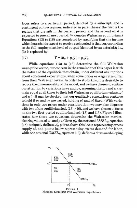
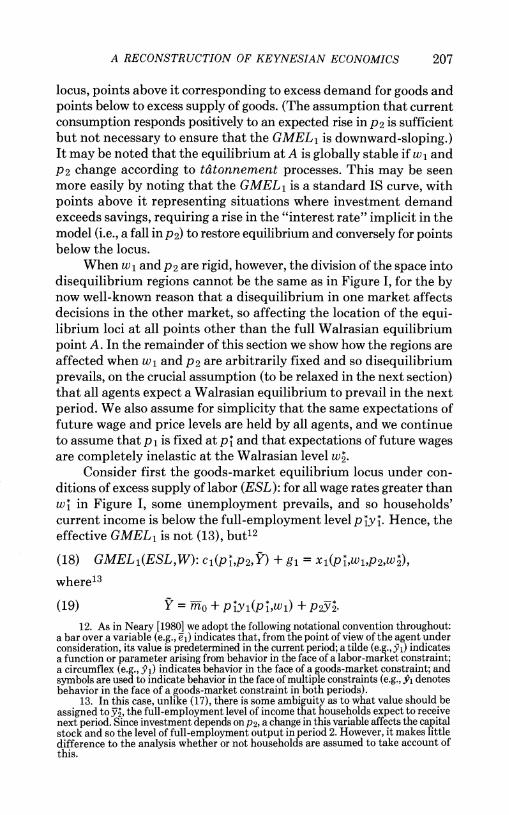
While equations (13) to (16) determine the full Walrasian wage-price vector, our concern in the remainder of this paper is with the nature of the equilibria that obtain, under different assumptions about constraint expectations, when some prices or wage rates differ from their Walrasian levels. In order to study this, it is desirable to reduce the dimensionality of the model, and we have chosen to confine our attention to variations in w1 and P2, assuming that P1 and w2 remain equal at all times to their full Walrasian equilibrium values, p and w . (It may be checked that our qualitative conclusions continue to hold if p 1 and w 1 are varied, holding p2 and w fixed.) With variations in only two prices under consideration, we may also dispense with two of the equilibrium loci, (13)-(16), and we have chosen to focus on the two first-period equilibrium loci, (13) and (15). Figure I illus- trates how these two equations determine the Walrasian market- clearing values of w1 and P2. Given p*, the notional LMEL1, equation (15), uniquely defines w*, points above this locus representing excess supply of, and points below representing excess demand for labor, while the notional GMEL1, equation (13), defines a downward-sloping

WI

ESL ESL EDG ESG

w* A LMEL

EDL I EDL ESG EDG

GMEL1

P2 PP

FIGURE I Notional Equilibria with Walrasian Expectations


locus, points above it corresponding to excess demand for goods and points below to excess supply of goods. (The assumption that current consumption responds positively to an expected rise in P2 is sufficient but not necessary to ensure that the GMEL1 is downward-sloping.) It may be noted that the equilibrium at A is globally stable if w1 and P2 change according to tatonnement processes. This may be seen more easily by noting that the GMEL1 is a standard IS curve, with points above it representing situations where investment demand exceeds savings, requiring a rise in the "interest rate" implicit in the model (i.e., a fall in P2) to restore equilibrium and conversely for points below the locus.

When w 1 and P2 are rigid, however, the division of the space into disequilibrium regions cannot be the same as in Figure I, for the by now well-known reason that a disequilibrium in one market affects decisions in the other market, so affecting the location of the equilibrium loci at all points other than the full Walrasian equilibrium point A. In the remainder of this section we show how the regions are affected when w1 and P2 are arbitrarily fixed and so disequilibrium prevails, on the crucial assumption (to be relaxed in the next section) that all agents expect a Walrasian equilibrium to prevail in the next period. We also assume for simplicity that the same expectations of future wage and price levels are held by all agents, and we continue to assume that P1 is fixed at p and that expectations of future wages are completely inelastic at the Walrasian level w*.

Consider first the goods-market equilibrium locus under conditions of excess supply of labor (ESL): for all wage rates greater than w 1 in Figure I, some unemployment prevails, and so households' current income is below the full-employment level p *y 1. Hence, the effective GMEL1 is not (13), but12

(18) GMEL1(ESL,W): cl(pp2,y) + g1 =Xl(P,Wl,P2,W2

where13

(19) Y = mO + p yi(p ,wi) + P2Y2-

12. As in Neary [1980] we adopt the following notational convention throughout: a bar over a variable (e.g., e1) indicates that, from the point of view of the agent under consideration, its value is predetermined in the current period; a tilde (e.g., Y1) indicates a function or parameter arising from behavior in the face of a labor-market constraint; a circumflex (e.g., 91) indicates behavior in the face of a goods-market constraint; and symbols are used to indicate behavior in the face of multiple constraints (e.g., Y1 denotes behavior in the face of a goods-market constraint in both periods).

13. In this case, unlike (17), there is some ambiguity as to what value should be assigned to Y*, the full-employment level of income that households expect to receive next period. Since investment depends on P2, a change in this variable affects the capital stock and so the level of full-employment output in period 2. However, it makes little difference to the analysis whether or not households are assumed to take account of this.


(18) (13)

W1\X \, C

K

(15) R

(21) (20) \(13)

P2

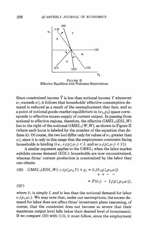
FIGURE II Effective Equilibria with Walrasian Expectations

Since constrained income Y is less than notional income Y whenever w1 exceeds w 1, it follows that households' effective consumption demand is reduced as a result of the unemployment they face, and so a point of notional goods-market equilibrium in (w1,p2) space corre- sponds to effective excess supply of current output. In passing from notional to effective regions, therefore, the effective GMEL1(ESL,W) lies to the right of the notional GMEL1( W, W), as shown in Figure II (where each locus is labeled by the number of the equation that defines it). Of course, the two loci differ only for values of w1 greater than wl, since it is only in this range that the employment constraint facing households is binding (i.e., e1(p*,wj) < L and so y1(p ,w1) < j).

A similar argument applies to the GMEL1 when the labor market exhibits excess demand (EDL): households are now unconstrained, whereas firms' current production is constrained by the labor they can obtain:

(20) GMEL1(EDL,W): CI(P ,P2,Y) + g1 = kl(l;p 1,P2,W )

= F(e1) -Il(P1,P2,W2),

(20')

where ei is simply L and is less than the notional demand for labor e1(p1,wi). We may note that, under our assumptions, the excess demand for labor does not affect firms' investment plans (assuming, of course, that the constraint does not become so severe that their maximum output level falls below their desired level of investment). If we compare (20) with (13), it must follow, since the employment


constraint bites, that effective supply is less than notional supply, implying that the constrained GMEL1 lies to the left of the notional locus when excess demand for labor prevails (i.e., when w1 is less than w as shown in Figure II.

The LMEL1 is affected in a similar manner when the goods market is out of equilibrium. Thus, in a situation of excess supply of goods, households are unconstrained, but firms are unable to make their notional level of sales. This forces them to recalculate their employment and investment decisions, with the result that the LMEL1 becomes

(21) LMEL1(ESG,W): L = ei[x ;wi1p2W ]

(21') = F-1[ I + Iiti;wip2,w2}], _-_ + -

where the current sales constraint facing firms is14

(22) xi = cI(p1,p2,Y) + g1 < X1(Pt,w1,P2,w2).

We may note that, by contrast with (8), current employment demand now depends on much more than just the current real wage: the demand for labor is determined both by what firms are able to sell and by what they decide to store. The latter is itself in turn affected by the sales constraint, by contrast with an employment constraint that, as equation (20') shows, does not affect the relative profitability of selling and investing. When we compare equations (15) and (21), since constrained employment demand el is less than notional employment demand e1 a point of notional labor-market equilibrium must corre- spond to effective excess supply of labor when excess supply of goods prevails; (21) therefore lies below (15) in Figure II. However, when we compare (21') with (20'), since constrained investment demand I, must be greater than notional investment demand II, it follows that these two loci do not coincide and that (21) lies to the left of (20). Al- lowing investment to be carried out by firms therefore leads to a region of effective excess supply of goods and excess demand for labor, or, in the terminology of Muellbauer and Portes [1978], a region of underconsumption.

14. As with other models of temporary equilibrium with rationing, though unlike the textbook Keynesian model, we assume that firms face a constraint on their sales net of investment demand, rather than on their gross sales. Otherwise, with only one representative firm using a single input to produce a homogeneous output, the corporate sector could never face strictly binding rations in both labor and goods markets, and so region U in Figure II would vanish.


Finally, when excess demand for goods prevails and the labor market is in equilibrium, firms are unconstrained, and, though households are rationed in the goods market, the assumption that labor is supplied inelastically ensures that this does not affect their labor supply. The effective LMEL1 therefore coincides with the notional locus (15): as shown in Figure II, the boundary between regions C and R does not pivot around point A.

These shifts from notional to effective equilibrium loci are summarized in Figure II (where the notional loci are shown as dashed lines and the effective loci as solid lines). Following now-standard usage, we may label the four regions K for Keynesian unemployment, C for classical unemployment, R for repressed inflation, and U for underconsumption. The nature of the disequilibrium in the two markets that prevails in each region is the same as in the corresponding notional regions in Figure j.15

IV. INTERTEMPORAL SPILLOVERS AND "BOOTSTRAPS"

EFFECTS

We now turn to the central focus of this paper: the effects of expectations by households or firms that they will face constraints in the future. One of the central concerns of the recent literature on fix-price models has been to show how a disequilibrium in one market has effects that spill over into other markets. In the light of this, it is not surprising that expectations of future constraints should have a significant effect on the behavior of firms and households in current markets. Our objective here, however, is more than simply to demonstrate that such intertemporal spillovers occur. We wish to show that they exhibit what we call a "bootstraps" property: households' expectations of future constraints on the sale of labor make it more likely that there will be a constraint on their ability to sell labor currently; while expectations by firms of constraints on their ability to sell goods in the future make it more likely that they will face a sales constraint in this period. It is this bootstraps property that leads to the possibility of there being multiple equilibria consistent with the same level of current wages and prices, and expected future wages and prices.

In this section we consider the general class of exogenously given

15. Figures I and II are in fact identical to the corresponding diagrams illustrating the regions of notional and effective equilibria in (w/p,m/p) space in the Barro- Grossman-Malinvaud model, provided it is assumed that labor is supplied inelastically and that investment may be carried out by firms.


constraint expectations. In the following section, the techniques that we have developed will be employed to investigate the special case where expectations are rational.16 Our strategy is to examine the effects of such expectations on the location of the various disequilibrium regions in (w1,p2) space. To illustrate the general points, we look in detail at two particularly interesting effects: those of expected Keynesian and classical unemployment on the location of the locus separating regions K and C (i.e., the GMEL, when current unemployment prevails).

The first point to emphasize is that if agents expect to be constrained next period this may affect their current behavior even if w1 and P2 are flexible; in other words, it may shift the notional equilibrium loci in Figure I. Admittedly, this is not true of the LMEL1, equation (15), since labor supply is fixed and, when firms face no constraints in the present period, their current employment decisions are determined only by P1 and w1, irrespective of what constraints they expect to face next period. However, the notional GMEL1 is affected. Consider first the case where agents expect regime K (excess supply of both labor and goods) to prevail next period. This displaces the notional locus for two distinct reasons. First, since households expect to be unemployed next period, their expected income is reduced, and so (13) must be replaced by

(23) GMEL1(W,ESL): c1(p ,P2,Y') + g1 =X1(p 1W1,P2,W2),

where

(24) Y- = rO + P1Y1 + P2y2, Y2 <Y2

The lowering of the income that households expect to receive next

16. In the context of a nonstochastic fix-price model, the particular sense in which the term rational expectations has come to be understood has extremely strong implications: all individuals have perfect foresight not only concerning the level of wages and prices that will prevail in the future and the constraints that will be binding, but also concerning the magnitude of those constraints. This degree of foresight seems highly implausible. A more general model would take into account explicitly the fact that individuals do not have point estimates of the constraints that they will face, but rather a probability distribution. Since the idiosyncratic components determining the precise distribution of the values of the constraints facing any one household or firm may be relatively large, the individual may have little basis on which to learn when his distribution differs from the "true" distribution. Moreover, since individuals are risk-averse and are typically unable to fully insure against the risks associated with facing particular constraints in the future, the certainty-equivalent value of the constraint may differ markedly from the mean value of the constraint. For these reasons, we conjecture that the discussion of this section may be of greater relevance than the more restricted assumption of rational expectations we employ in the next section. However, not all readers have agreed with us, and, for those readers, the present section should be viewed as simply developing the analytical tools that will be employed in the next.


(23) (25) (28) WI I

(27)\

-- A ---~~~~~~(15)

I(26)

1. (23) _______ (1o 3)

pF p pH P2 2 2 2

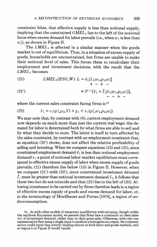
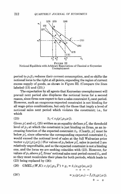
FIGURE III Notional Equilibria with Arbitrary Expectations of Classical or Keynesian

Unemployment

period to P2Y2 reduces their current consumption, and so shifts the notional locus to the right at all points, expanding the region of current excess supply of goods, as shown in Figure III. (Compare the lines labeled (13) and (23).)

The expectation by all agents that Keynesian unemployment will prevail next period also displaces the notional locus for a second reason, since firms now expect to face a sales constraint x2 next period. However, such an exogenous expected constraint is not binding for all wage-price combinations, but only for those that imply a level of notional sales next period which violates the constraint; i.e., for which

(25) X2 < X2(PP2,W2)-

Given p and w , (25) written as an equality defines pF, the threshold level of P2 at which the constraint is just binding on firms, as an increasing function of the expected constraint x2. (Clearly, pF must lie below p*, since otherwise the corresponding expected constraint x2 would exceed the notional level of sales at the full Walrasian price vector X2(p1,p2,W2).) For values of P2 below pF, sales in period 2 are relatively unprofitable, and so the expected constraint is not a binding one, and the locus we are seeking coincides with (23). However, for values of P2 above p F, firms' notional sales next period exceed x2, and so they must recalculate their plans for both periods, which leads to (23) being replaced by (26):

(26) GMELi(W,K): Cl(P*,P2,2") + g1 =1(X2;P*WlW2)

(26') = Y1(P1,w41) -Il(y2;p1,W2)

+-+


The expected sales constraint reduces current investment and so "spills over" into an increase in current sales causing the region of excess supply of goods to expand. This is shown in Figure III by the counterclockwise pivoting of (23) around point B (the point at which the constraint (25) is just binding).

The effect on the notional GMEL1 of the expectation that classical unemployment will prevail next period may be determined in a similar manner, the main difference being that firms do not now expect to face any constraints and so remain on their notional sales function. Households, on the other hand, expect to be constrained in both markets. We assume that their expectation of unemployment is the same as that already assumed in our discussion of expected Keynesian unemployment (i.e., the income they expect to receive in periods 1 and 2 is given by (24)). As before, therefore, this shifts the locus from (13) to (23). In addition, households expect to be rationed in their goods purchases, causing them to recalculate their current demand with the result that (23) must be replaced by (27):

(27) GMEL1(WC): c6(c2;pLtp29Y) + g1 = X1(P9,w1,P2,W2*) - -? +

The expected goods constraint j2 reduces the incentive to save and so raises households' current demand, shifting the notional GMEL1 to the left and expanding the region of current excess demand for output. However, as with the expected sales constraint in (26), this does not happen for all (w1,p2) combinations but only for those at which the expected constraint -2 is binding; i.e., for which

(28) c2 < c2(pp2,Y).

Given pt, (28) written with equality defines pH, the threshold level OfP2 at which the expected constraint U2 is just binding on households, as a decreasing function of c2. As illustrated in Figure III, p1 must lie to the right of p*; for values of P2 above pf notional demand for consumption in period 2 is less than the constraint, and (23) coincides with (27). However, for lower values of P2, households expect to be constrained and so the notional GMEL 1 pivots to the left around point D (the point on (23) at which P2 equals p2).

The major conclusion to be drawn from Figure III is that the notional GMEL 1 when classical unemployment is expected next period lies strictly to the left of the notional GMEL1 when Keynesian unemployment is expected. Before noting the implications of this, we must recall that our main concern is not with the location of various notional loci in the diagram but rather with the location of the corresponding effective loci when different expectations are held about


(23) (3)

(30) WI ~~~K, K) (CK)

" or or

( (,C) (C,C)

(27)~~~~~~23

(KAK~ or N,'

(KGC) N

A XN~~ A"N (15) A~~~

" (26)

(23)

P2

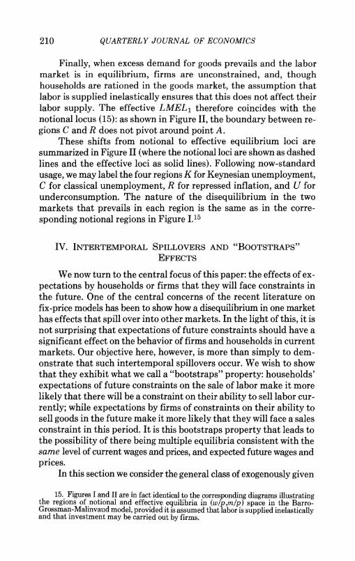
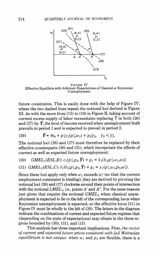
FIGURE IV Effective Equilibria with Arbitrary Expectations of Classical or Keynesian

Unemployment

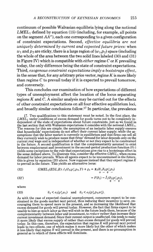
future constraints. This is easily done with the help of Figure IV, where the two dashed lines repeat the notional loci derived in Figure III. As with the move from (13) to (18) in Figure II, taking account of current excess supply of labor necessitates replacing Y in both (26) and (27) by Y, the level of income received when unemployment both prevails in period 1 and is expected to prevail in period 2:

(29) Y= meo + p*y(pt,w1) + P2Y2, Y2 <Y2.

The notional loci (26) and (27) must therefore be replaced by their effective counterparts (30) and (31), which incorporate the effects of current as well as expected future unemployment:

(30) GMEL1(ESL,K): cl(pP2,) + g1 = (2;P1WW2)

(31) GMEL1(ESL,C): 61(c2;PTP2,) + g1 = x1(p*,wbp2,w2).

Since these loci apply only when w1 exceeds wt (so that the current employment constraint is binding), they are derived by pivoting the notional loci (26) and (27) clockwise around their points of intersection with the notional LMEL1, i.e., points A' and A". For the same reasons just given that require the notional GMEL1 when classical unemployment is expected to lie to the left of the corresponding locus when Keynesian unemployment is expected, so the effective locus (31) in Figure IV must lie wholly to the left of (30). The letters in the diagram indicate the combinations of current and expected future regimes that (depending on the state of expectations) may obtain in the three regions bounded by (30), (31), and (15).

This analysis has three important implications. First, the vector of current and expected future prices consistent with full Walrasian equilibrium is not unique: when w1 and P2 are flexible, there is a


continuum of possible Walrasian equilibria lying along the notional LMEL1 defined by equation (15) (including, for example, all points on the segment AA"), each one corresponding to a given configuration of constraint expectations. Second, effective equilibria are not uniquely determined by current and expected future prices: when w1 and P2 are sticky, there is a large region of (w1,p2) space (including the whole of the area between the two solid lines labeled (30) and (31) in Figure IV) which is compatible with either regime C or K prevailing today, the only difference being the state of constraint expectations. Third, exogenous constraint expectations imply a bootstraps effect, in the sense that, for any arbitrary price vector, regime K is more likely than regime C to prevail today if it is expected to prevail tomorrow, and conversely.

This concludes our examination of how expectations of different types of unemployment affect the location of the locus separating regions K and C. A similar analysis may be carried out for the effects of other constraint expectations on all four effective equilibrium loci, and broadly similar conclusions follow.17 In particular, the prevalence

17. Two qualifications to this statement must be noted. In the first place, the LMEL1 under conditions of excess demand for goods turns out to be completely independent of the state of expectations about future constraints, just as we found in the last section that with Walrasian expectations it coincides with the notional LMEL1. The reasons for this are simple: the assumption of an inelastic labor supply ensures that households' expectations do not affect their current labor supply; while the assumptions that the labor market is currently in equilibrium and that firms can sell all they currently wish to produce mean that firms' demand for labor depends only on the current real wage and is independent of whether or not they expect to be constrained in the future. A second qualification is that the complementarity assumed to exist between employment and investment in the second-period production function H(-) yields some exceptions to the rule that expectations give rise to a bootstraps effect in the sense defined above. To illustrate this, consider the effective GMEL1 when excess demand for labor prevails. When all agents expect to be unconstrained in the future, this is given by equation (20) above. Now suppose instead that they expect regime R to prevail in the future. This yields an alternative locus:

(32) GMEL,(EDL,R): 61(ZT2;plp2,Y) + g1 = 91(JbJ2;,p2)

(32') = F(J-) - I1(J2;pI,p2),

where

(33) e- < ei(p*,wl) and e2 < e2(P*,p2,w*). As with the case of expected classical unemployment, consumers expect to be constrained in the goods market next period, thus reducing their incentive to save, en- couraging them to spend more in the present, and so increasing the likelihood that excess demand for goods will prevail today. However, the fact that firms expect to be unable to hire as much labor as they will wish in the future leads them, because of the complementarity between labor and investment, to reduce rather than increase their current investment demand. Since their current output is unaffected, this tends to make it more likely that excess supply of rather than excess demand for goods will prevail today. In this case, therefore, the expectation that regime R will prevail next period leads to two effects, one of which makes it more likely but the other of which makes it less likely that regime R will prevail in the present, and there is no presumption in general as to which of these effects will dominate.


of a given regime today depends on the expectations held about which regimes will prevail tomorrow, and in most cases these expectations give rise to bootstraps phenomena in the sense already discussed.

V. RATIONAL CONSTRAINT EXPECTATIONS

The analysis in the previous section is open to the criticism that, by placing no restrictions on agents' expectations of future constraints, it makes inevitable a considerable degree of arbitrariness in the current regimes that are consistent with a given wage-price vector. In this section we explore an alternative approach that avoids this arbitrariness of expectations by postulating that households and firms have full information concerning each others' intended future actions. Thus, for example, the income constraint that households expect to face in the next period equals the value of output that firms currently intend to produce in that period. By analogy with the widely studied phenomenon of rational expectations of prices, we label this hypothesis one of rational constraint expectations (RCE). The concept of rational constraint expectations clearly has a considerable informational requirement. However, it is only assumed that agents know the aggregate constraints that they will face next period: for example, from equation (34) below, firms know what the level of aggregate demand will be next period, but they do not know its distribution between different consumers. This assumption is not only plausible but is also necessary if the hypothesis of price-taking behavior in the face of fixed prices is to be maintained, since if firms knew the de- mands of individual consumers they would have an incentive to enter into bilateral bargaining with them.

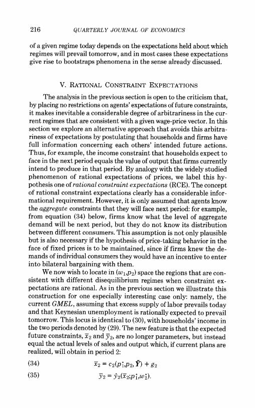
We now wish to locate in (w1,p2) space the regions that are consistent with different disequilibrium regimes when constraint expectations are rational. As in the previous section we illustrate this construction for one especially interesting case only: namely, the current GMEL, assuming that excess supply of labor prevails today and that Keynesian unemployment is rationally expected to prevail tomorrow. This locus is identical to (30), with households' income in the two periods denoted by (29). The new feature is that the expected future constraints, x2 and Y2, are no longer parameters, but instead equal the actual levels of sales and output which, if current plans are realized, will obtain in period 2:

(34) x2= c2(p 1,p2, I) + g2

(35) Y2 = Y2(X2;pw 2)


W ~~(18) (C) RCE wl~~~~(C,W ) or C (KW) or \ \ (K,K;RCE) (K,K;RCE) \ \(CW)or

'... \M\A(CK; RCE)

- -~~~~~A (36)' ~~~~ \

\ 36)

\ (37) (37)*

P2 FIGURE V

Effective Equilibria with Rational Expectations of Keynesian Unemployment

The main result we wish to establish concerning the GMEL 1 with current unemployment and rational expectations of Keynesian unemployment is that, when this locus exists, it must lie to the right of (18), the GMEL1 with current unemployment, and Walrasian expectations. To see this, consider the following algorithm for determining the location of the desired locus: for each value of x2, the expected future sales constraint, locate in (w1,p2) space the following two loci, which are derived from equations (30) and (34), by using equations (29) and (35) to eliminate Yand Y2:

(36) cj[pt,p2,M0 + pTyA(pLwO) + p2Y2(X2;ptw2)I + g1 = X(X2;plw1,w) 2

(37) x2 = cJ[ppP2Mo + p*yI(pIwL) + P2,Y2(X2;P*,W2)] + g2.

Now trace out the locus of intersection points of (36) and (37) as x2

is varied parametrically. It is clear that this locus is the RCE locus we require, since (36) is the GMEL1 with current unemployment and expected Keynesian unemployment conditional on a given sales constraint being expected by both firms and households, while (37) states that that sales constraint equals planned aggregate demand next period. Thus, every point on the RCE locus must lie on one of the family of loci defined by (36). But, as argued in Section IV, if the expected sales and income constraints, x2 and Y2, are binding, then excess supply of goods in period 1 is increased. Hence every locus defined by (36) for different binding values of -2 must lie to the right of (18), the corresponding locus when no binding constraints are expected next period. Thus, the RCE locus itself must lie to the right of (18), as was to be proved.

This reasoning is illustrated in Figure V. The dashed lines labeled


(36)* and (37)* represent the loci defined by equations (36) and (37) where the expected sales constraint equals the value of actual sales next period in the full Walrasian equilibrium: c2(p 1,p 2,i + p 1Y + P 2Y2) + g2. These loci intersect at A, since the full Walrasian equilibrium may be interpreted as a "constrained" equilibrium where the values of current and expected future constraints equal the actual values that obtain in the full Walrasian equilibrium itself. Hence point A lies on the GMEL1 with rational constraint expectations. A reduction in the expected sales constraint below its Walrasian level shifts both curves upward to (36)' and (37)', whose intersection point E therefore lies on the RCE locus.18 Successive variations in x2 thus trace out the required locus (labeled "RCE" in the diagram) that must lie to the right of (18) if the rationally expected future sales constraint is a binding one.

The implication of this result is of considerable interest: the set of (w1,p2) combinations consistent with Keynesian rather than classical unemployment in the current period is greater when Keynesian unemployment is rationally expected to prevail next period than when Walrasian equilibrium is expected. In this sense we may say that rational constraint expectations increase the likelihood that Keynesian unemployment will prevail in the current period. At the same time, the requirement that expectations be rational places more restrictions on the types of equilibria consistent with a given wage-price vector than did the exogenous constraint expectations considered in Section IV: for example, many points such as A" are consistent with Keynes- ian unemployment in the current period if expectations are allowed to be arbitrarily pessimistic, but not in general if they are required to be rational.

The implications of rational constraint expectations for the location of other equilibrium loci may be considered in a similar fashion, and the same conclusion follows: since every point on a RCE locus must coincide with a point on the locus that represents the same combination of current and expected future regimens but contingent on exogenously given expected constraints, the conclusions in Section IV concerning the location of equilibrium loci when constraint expectations are arbitrary continue to hold when they are rational. Hence, subject to the qualification noted in footnote 17 at the end of Section IV arising from the complementarity between investment and

18. It is possible that E lies to the left of (18), in which case the solution to equations (36) and (37) does not satisfy the required inequality constraints; i.e., the effective GMEL1 with rational expectations of Keynesian unemployment does not exist.


WI

B A

P2

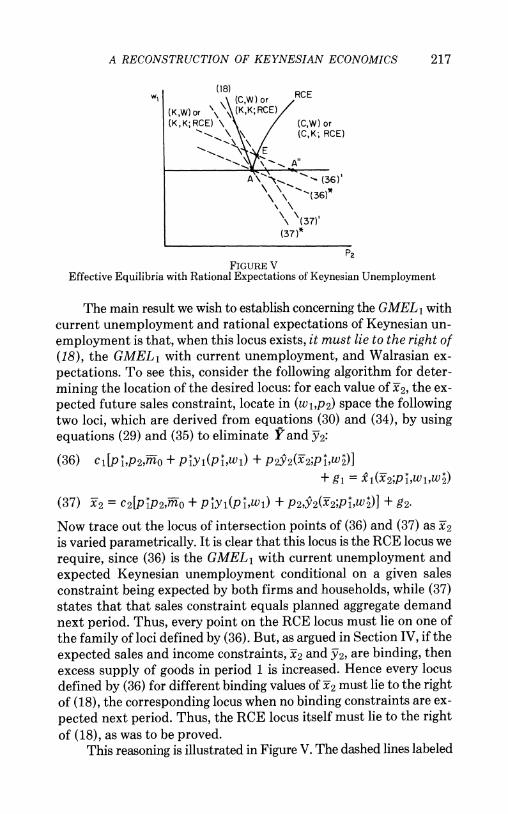
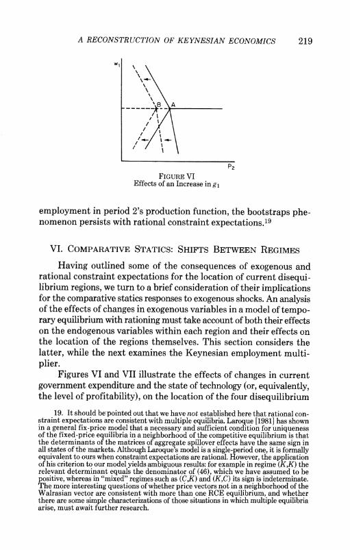
FIGURE VI Effects of an Increase in g,

employment in period 2's production function, the bootstraps phenomenon persists with rational constraint expectations'

VI. COMPARATIVE STATICS: SHIFTS BETWEEN REGIMES

Having outlined some of the consequences of exogenous and rational constraint expectations for the location of current disequilibrium regions, we turn to a brief consideration of their implications for the comparative statics responses to exogenous shocks. An analysis of the effects of changes in exogenous variables in a model of temporary equilibrium with rationing must take account of both their effects .on the endogenous variables within each region and their effects on the location of the regions themselves. This section considers the latter, while the next examines the Keynesian employment multiplier.

Figures VI and VII illustrate the effects of changes in current government expenditure and the state of technology (or, equivalently, the level of profitability), on the location of the four disequilibrium

19. It should be pointed out that we have not established here that rational constraint expectations are consistent with multiple equilibria. Laroque [1981] has shown in a general fix-price model that a necessary and sufficient condition for uniqueness of the fixed-price equilibria in a neighborhood of the competitive equilibrium is that the determinants of the matrices of aggregate spillover effects have the same sign in all states of the markets. Although Laroque's model is a single-period one, it is formally equivalent to ours when constraint expectations are rational. However, the application of his criterion to our model yields ambiguous results: for example in regime (K,K) the relevant determinant equals the denominator of (46), which we have assumed to be positive, whereas in "mixed" regimes such as (CK) and (K,C) its sign is indeterminate. The more interesting questions of whether price vectors not in a neighborhood of the Walrasian vector are consistent with more than one RCE equilibrium, and whether there are some simple characterizations of those situations in which multiple equilibria arise, must await further research.


WI ~ ~ I

P2

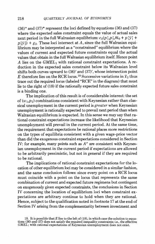
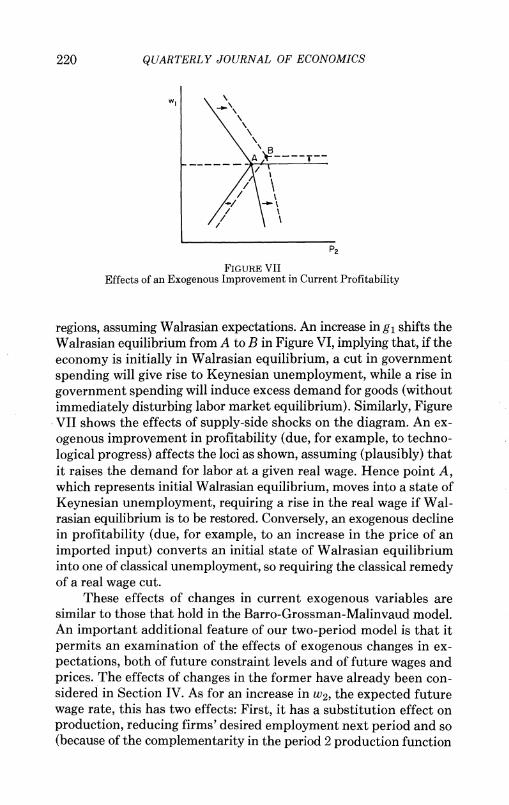
FIGURE VII Effects of an Exogenous Improvement in Current Profitability

regions, assuming Walrasian expectations. An increase in g, shifts the Walrasian equilibrium from A to B in Figure VI, implying that, if the economy is initially in Walrasian equilibrium, a cut in government spending will give rise to Keynesian unemployment, while a rise in government spending will induce excess demand for goods (without immediately disturbing labor market equilibrium). Similarly, Figure VII shows the effects of supply-side shocks on the diagram. An exogenous improvement in profitability (due, for example, to techno- logical progress) affects the loci as shown, assuming (plausibly) that .it raises the demand for labor at a given real wage. Hence point A, which represents initial Walrasian equilibrium, moves into a state of Keynesian unemployment, requiring a rise in the real- wage if Wal- rasian equilibrium is to be restored. Conversely, an exogenous- decline in profitability (due, for example, to an increase in the price of an imported input) converts an initial state of Walrasian equilibrium into one of classical unemployment, so requiring the classical remedy of a real wage cut.

These effects of changes in current exogenous variables are similar to those that hold in the Barro-Grossman-Malinvaud model. An important additional feature of our two-period model is that it permits an examination of the effects of exogenous changes in expectations, both of future constraint levels and of future wages and prices. The effects of changes in the former have already been considered in Section IV. As for an increase in W2, the expected future wage rate, this has two effects: First, it has a substitution effect on production, reducing firms' desired employment next period and so (because of the complementarity in the period 2 production function


H(-)) reducing current investment demand and therefore raising the current supply of output. Second, to the extent that households foresee the wage increase and the consequent reduction in output next period, their lifetime income is reduced, and so their current demand is lowered. On both counts, therefore, a rise in w2 expands the region of excess supply of current output. Of course, this conclusion relies heavily on the assumed absence of distribution effects: if the marginal propensity to consume out of wages exceeds that out of nonlabor income, then an increase in w2 could raise demand for output in period 1. To the extent that this effect dominated, an increase in w2 would have exactly the same effect on the diagram as an increase in g1 in Figure VI, implying that an expected future wage cut will shift the economy from Walrasian equilibrium into Keynesian unemployment in the current period.

The relationships illustrated in Figures VI and VII between changes in exogenous variables and shifts in the equilibrium loci continue to hold whatever assumptions are made about constraint expectations. In addition, rational constraint expectations permit a further role for demand- and supply-side shocks through the "an- nouncement effects" of perfectly foreseen changes in the levels of future government spending and profitability. Thus, an increase in g2 relaxes the expected future sales constraint on firms, which both raises their current investment demand and (by raising their planned output next period) relaxes the income constraint facing households. On both counts, the region of excess demand for current output is enlarged, and so with rational constraint expectations a perfectly anticipated increase in g2 has exactly the same effect on the diagram as an increase in g, has in Figure VI. Similarly, an anticipated increase in future profitability enlarges the region of current excess supply of goods, and so has effects similar to those of an increase in current profitability in Figure VII.

VII. COMPARATIVE STATICS: THE KEYNESIAN EMPLOYMENT MULTIPLIER

Turning next to the comparative statics properties of the model within different regions, we show in this section that, when households and firms have rational expectations of future constraints, the employment multiplier following an increase in government spending is larger than conventionally assumed.20 To see this, consider first

20. The calculation of other comparative statics results, many of which are similar to those found in earlier studies of the Barro-Grossman-Malinvaud model, is left to the interested reader.


the multiplier when Keynesian unemployment prevails in the current period, but agents make no allowance for future constraints (i.e., they assume that Walrasian equilibrium will prevail next period). Current employment and sales are therefore jointly determined by equations (38), (39), and (40):

(38) l= el(X-l;Wl9P29W2)

(39) xi= c1(plp2J) + g1

(40) V = mo + plS'l(Xl;plp2,w2) + P2Y2-

These imply a simple one-period multiplier, very similar to the usual textbook expression:21

(41) g J o I

However, if regime K both prevails today and is rationally expected to prevail tomorrow, then since all agents take into account the effect of current events on future behavior, (38), (39), and (40) must be replaced by the following set of four equations:

(42) e= Xi( X,2;wiw2)

(43) xi = cl(plp2,f) + g1

(44) x2 = c2(plp2, Y) + g2

(45) Y = Yo + p1i i(xix2;wlw2) + p2y2(XlX2;wlw2).

Routine calculations show that under these circumstances the multiplier is

(46) oL = [I - cAl -c2A2

691 by [by ~ 2 ?eiJC X i I - A2i+ - 1 ,

where

(47) Al =P1 + P2- oX1 dx1 dx

(48) A2= =Pi +P2-X oX2 oX2 X2

21. The difference between (41) and the usual textbook expression arises solely from the assumption in our model that the corporate sector faces a constraint on its sales net of investment purchases rather than on its gross sales.


There are three distinct reasons why (46) exceeds (41).22 First, as shown in the Appendix, Ze 6i/xi exceeds el/lb1 (at least locally); i.e., a relaxation of the current sales constraint faced by firms has a greater impact effect on their current demand for labor when they expect to face a similar constraint in the future than when they expect to be unconstrained. This result, which reflects the Samuelson-Le Chatelier principle, does not arise because expectations are rational but solely because they are "Keynesian": hence government policy has a greater expansionary effect when firms are pessimistic about their future sales prospects. Second, a relaxation of the current sales constraint also causes firms to revise their future employment and output plans upward, but with rational constraint expectations, households know that this raises their lifetime income, and so they increase their consumption in both periods, thus having a further impact effect on firms' current demand for labor. Third, each of these impact effects (represented by 61/.YT1 and eI/x2, respectively) gives rise to a multiplier chain within each period accentuated by accelerator-type effects between the two periods, as the relaxation of a constraint in one period on one group of agents has an enhanced expansionary effect by relaxing the constraints that the other group faces in the current period and expects to face next period.23 The net effect of these interactions is to raise the multiplier considerably: for example, the coefficient of a i/?l.Y in (46) exceeds that of ?e1/?x in (41).

To summarize, we have demonstrated that when Keynesian unemployment prevails in the current period, the employment multiplier is greater with rational than with static expectations of Keynesian unemployment, and greater still than with Walrasian expectations. These conclusions may be supplemented by two additional observations. First, the efficacy of government policy shown by (46) does not follow from its being unanticipated. On the contrary, a perfectly anticipated increase in government spending in period 2 has a similar expansionary effect. Second, the rigidity of current and expected future prices and wages is not necessary for government spending to have real effects in this model: by changing the division of national output between public and private consumption, a rise

22. The denominator of (46) may reasonably be assumed to be positive, since it equals the responsiveness of income Yto a change in initial money balances m-o. If this were negative, then with fixed prices and wages the model would be unstable under a quantity-tdtonnement adjustment process.

23. The effect of expected sales constraints in giving rise to an income-investment accelerator was pointed out in a partial-equilibrium model by Grossman [1972] and in a simple general-equilibrium model by Akerlof and Stiglitz [1965].


in g, has real effects even in the flexible-price equilibrium described by equations (13) to (16). However, the same is not true of monetary expansion: in full Walrasian equilibrium an increase in initial money balances merely raises all nominal magnitudes by the same propor- tionate amount, leaving output and employment unchanged, whereas when wage and price rigidities give rise to current and rationally anticipated Keynesian unemployment, it has real effects similar to (46):

(49) 1= i- 1A - A2 A 1- 1 a + a c21 )M_ [ by I -Xi bY Cx2 (YJ

These findings illustrate the important point that the implications of rational expectations for the effectiveness of government policy depend completely on whether or not they are accompanied by sufficient price flexibility to ensure market clearing without rationing. When prices are rigid, rational constraint expectations, at least in the present model, actually enhance the effectiveness of anticipated government policy.

VIII. SUMMARY AND CONCLUSION

This paper has presented a simple two-period model of temporary equilibrium with rationing that lays considerable stress on agents' expectations of the constraints that they may face in the future. Ar- bitrary constraint expectations were shown to permit multiple equilibria, with more than one regime in the present period being consistent with a given vector of current and expected future wages and prices. Moreover, such expectations were shown to exhibit a "bootstraps" property, so that, for example, Keynesian unemployment is more likely than classical unemployment to prevail today if it is expected to prevail tomorrow, and vice versa.

It was also shown that Walrasian equilibrium and the impotence of government policy are not guaranteed by rational constraint expectations, in the sense of perfect foresight of future constraint levels. On the contrary, such expectations actually increase the probability that Keynesian unemployment will prevail today relative to Walrasian expectations, and they raise the value of the government multiplier. These results suggest that the critique of the effectiveness of government policy presented by "new classical macroeconomists," such as Sargent and Wallace [1975], rests primarily on their assumption


that wages and prices move instantaneously to clear markets, and not on their use of the rational expectations hypothesis.24

One possible objection to our concept of rational constraint expectations is that with so much information available, agents should be able to change prices directly to attain the Walrasian equilibrium. We believe, however, that this type of argument greatly underesti- mates the difficulties of coordinating individual behavior in a de- centralized economy with highly imperfect information. In such an environment the two assumptions of rational expectations and wage-price flexibility are by no means equivalent. Even the assumption of rational constraint expectations alone has an almost unbelievable informational requirement; we defend it not on the grounds of descriptive realism, but because it isolates the role of wage-price rigidities (including rigidities in expected future wages and prices) in giving rise to unemployment, intermarket spillovers, and other such Keynesian phenomena.

Finally, we would argue that even though wage-price flexibility may eventually bring the economy to Walrasian equilibrium, it is unlikely to do so by a swift or easy route. The facts that shifts in expectations may bring about substantial changes in the wage-price vector required to achieve Walrasian equilibrium, and that the market whose price is sticky need not be the one that fails to clear, suggest a sort of "dynamic second-best theorem": with limited flexibility of some prices, increasing the flexibility of other prices may reduce rather than increase the ability of the system to return to Walrasian equilibrium. A fuller consideration of such dynamic problems, as well as an evaluation of the ability of the real-balance effect-excluded from consideration in this paper-to ensure the reattainment of equilibrium, are topics to which we hope to return.

APPENDIX: THE BEHAVIOR OF THE FIRM

The behavior of the firm under different constraint regimes can be derived directly by maximizing (5) subject to (6), (7), and appro- priate additional constraints, but it is easier and more illuminating to adopt a dual approach, along with the concept of "virtual" prices used by Neary and Roberts [1980].

Consider first the case of no constraints in either period, where the unconstrained profit function is defined as follows. (To simplify notation, we denote the price-wage vector by (p,w,q,v) in this Ap-

24. Similar criticisms have been made by Fischer [1977] and Phelps and Taylor [1977].


pendix, and not by (p1,wl,p2,w2) as in the text):

(A.1) ir(p,w,q,v) = max [p{F(e1) - I,} - we, el,e2,Il,I2

+ q{H(e2,1l) - I2} - ve2 + (I2;0)].

By Hotelling's Lemma the partial derivatives of this function give the firm's unconstrained net sales and employment demand functions in each period: (A.2) xrp , x rw = -el, Irq = X2, 1rv = -e2. The properties of these functions may be deduced in standard fashion by noting that wx is a convex function of all prices (i.e., iy,, > 0, ,u = pwqv). These properties may be further simplified by observing that (in the absence of additional constraints) the firm's decision problem is separable into three distinct subproblems:

(A.3) r(p,w,q,v) = irl(pw) + ir2(p,q,v) + ir3(q)

(A.4) = max [pF(e1) - we1] + max [qH(e2,Il) el Ile2

- p'l - ve2I + max [(2) - qI2] 12

Hence current employment demand is independent of period 2 prices and wages and depends only on the current real wage wip:

(A.5) 7rwA = r = O = q,v.

Suppose now that the firm faces a sales constraint in the current period: xi < xi. Its behavior in this case may be deduced from the constrained function i(x-l;p,w,q,v), and as in Neary and Roberts [1980], the properties of the latter are most easily determined by re- lating it to the unconstrained profit function evaluated at the virtual price p:

(A.6) (x-l;p,w,q,v) = max [ir(p,w,q,v): x, < Yl]

(A.7) = ir(j-,w,q,v) + (p - p-)x-,

where the virtual price, that price which would induce an unconstrained firm to produce Yl, is defined implicitly by

(A.8) xi = 7rp (p-,w q v)

It is easily seen that the constrained and unconstrained current employment demand functions coincide when the latter is evaluated at the virtual price p-:

(A.9) e1= -w = -Irw - (irp - yl) (w = -wxw.

Hence the effect of a change in the sales constraint on current employment demand is found from (A.9) and (A.8) to be

(A.10) a = -7rWP


(A.11) = -Wwp7rAp > 0.

Other properties of the firm's behavior in the face of the sales constraint may be deduced in a similar manner. For example,

(A.12) l= -ir - i

(A.13) - ,be + ir PP rpw

Since the second term in (A.13) is positive, this yields a Le Chatel- ier-type result: the imposition of a sales constraint reduces (at least locally) the responsiveness of employment demand to a change in wages.

Consider next the case where the firm faces a sales constraint in both periods: x1 < xi and x2 < x2. We may proceed in an analogous fashion to define a doubly constrained profit function:

(A.14) 7(xl,2;pow~qv) = max[r(Yl;p,wqv): X2 < X21

(A.15) = *x;pwf,) + (q - #)2

(A.16) = Jr(pw ,,v) + (p - P)xl + (q - OY2- The two virtual prices, T and ?, corresponding to the two constraints, x1 and x2, are now jointly determined by (A.8) (with if replacing q) and (A.17):

(A.17) x2 = 7rq(h,w, qV).

As before, the doubly constrained and unconstrained labor demand functions coincide when the latter is evaluated at jY and V:

(A.18) e = A

Hence,

(A.19) Ix =rwq_

This may be simplified by recalling from (A.5) that Wxwq is zero and by solving (A.8) and (A.17) for bY/&l. This yields

(A.20) Nil= -amp [pp - 1rpq7rpprqp>1,

This is clearly greater than (A.11), which proves that (as was asserted in Section VI) the presence of an expected future sales constraint increases the responsiveness of current employment demand to a relaxation of the current-sales constraint.

It should be clear how these techniques may be used to deduce the behavior of the firm in the presence of other combinations of constraints.

UNIVERSITY COLLEGE, DUBLIN

PRINCETON UNIVERSITY


REFERENCES Akerlof, G. A., and J. E. Stiglitz, "Investment and Wages," read at the Econometric

Society Meeting, New York, 1965. Barro, R. J., and H. I. Grossman, "A General Disequilibrium Model of Income and

Employment," American Economic Review, LXI (1971), 82-93. , and , Money, Employment and Inflation (Cambridge: Cambridge University Press, 1976).

Benassy, J. P., "Neo-Keynesian Disequilibrium in a Monetary Economy," Review of Economic Studies, XLII (1975), 503-23.

Blad, M. C., and A. P. Kirman, "The Long-Run Evolution of a Rationed Equilibrium Model," University of Warwick Economic Research Paper No. 128, 1978.

B6hm, V., "Disequilibrium Dynamics in a Simple Macroeconomic Model," Journal of Economic Theory, XVII (1978), 179-99.

Clower, R. W., "The Keynesian Counter-Revolution: A Theoretical Appraisal," in F. H. Hahn and F. Brechling, eds., The Theory of Interest Rates (London: Mac- millan, 1965).

Dehez, P., and J. J. Gabszewicz, "Savings Behaviour and Disequilibrium Analysis," Colloques Internationaux du C.N.R.S., No. 259 (1978),197-212; CORE Reprint No. 313.

Dixit, A. K., "Public Finance in a Keynesian Temporary Equilibrium," Journal of Economic Theory, XII (1976), 242-58.

-, "The Balance of Trade in a Model of Temporary Equilibrium with Rationing," Review of Economic Studies, XLV (1978), 393-404.

Fischer, S., "Long-term Contracts, Rational Expectations, and the Optimal Money Supply Rule," Journal of Political Economy, LXXXV (1977), 191-210.

Grandmont, J. M., "Temporary General Equilibrium Theory," Econometrica, XLV (1977), 535-73. , Money and Value (Cambridge: Cambridge University Press, 1982).

Grossman, H. I., "A Choice-Theoretic Model of an Income-Investment Accelerator," American Economic Review, LXII (1972), 630-41.

Hansen, B., A Study in the Theory of Inflation (London: Allen and Unwin, 1951). Hicks, J. R., The Crisis in Keynesian Economics (Oxford: Basil Blackwell, 1974). Hildenbrand, K., and W. Hildenbrand, "On Keynesian Equilibria with Unemployment

and Quantity Rationing," Journal of Economic Theory, XVIII (1978), 255-77. Honkapohja, S., "On the Dynamics of Disequilibria in a Macro Model with Flexible

Wages and Prices," in M. Aoki and A. Marzello, eds., New Trends in Dynamic Systems Theory and Economics (New York: Academic Press, 1979), pp. 303- 36.

Hool, B., "Monetary and Fiscal Policies in Short-Run Equilibria with Rationing," International Economic Review, XXII (1980), 301-16.

Laroque, G., "On the Local Uniqueness of the Fixed Price Equilibria," Review of Economic Studies, XLVIII (1981), 113-29.

Leijonhufvud, A., On Keynesian Economics and the Economics of Keynes (New York: Oxford University Press, 1968).

Malinvaud, E., The Theory of Unemployment Reconsidered (Oxford: Basil Blackwell, 1977).

Muellbauer, J., and R. Portes, "Macroeconomic Models with Quantity Rationing," Economic Journal, LXXXVIII (1978), 788-821.

Neary, J. P., "Nontraded Goods and the Balance of Trade in a Neo-Keynesian Tem- porary Equilibrium," this Journal, XCV (1980), 403-29. , and K. W. S. Roberts, "The Theory of Household Behavior under Rationing," European Economic Review, XIII (1980), 25-42.

Patinkin, D., Money, Interest and Prices: An Integration of Monetary and Value Theory, 2nd ed. (New York: Harper and Row, 1965).

Phelps, E. S., and J. B. Taylor, "Stabilizing Powers of Monetary Policy with Rational Expectations," Journal of Political Economy, LXXXV (1977), 163-90.

Sargent, T. J., and N. Wallace, " 'Rational' Expectations, the Optimal Monetary In- strument, and the Optimal Money Supply Rule," Journal of Political Economy, LXXXIII (1975), 241-54.

Solow, R. M., and J. E. Stiglitz, "Output, Employment and Wages in the Short Run," this Journal, LXXXII (1968), 537-60.

Stiglitz, J. E., Lectures in Macroeconomics (All Souls' College, Oxford: 1978).

Toward a Reconstruction of Keynesian Economics ...

Documents

Transcript of Toward a Reconstruction of Keynesian Economics ...