Torsion and shear stresses due to shear centre eccentricity

in SCIA Engineer

Delft University of Technology

Marijn Drillenburg

October 2017

Contents

1 Introduction 21.1 Hand Calculation . . . . . . . . . . . . . . . . . . . . . . . . . . . . . . . . . . . . 21.2 Results in SCIA . . . . . . . . . . . . . . . . . . . . . . . . . . . . . . . . . . . . . 4

2 Investigation Plan 6

3 Geometry 73.1 I-shaped cross section . . . . . . . . . . . . . . . . . . . . . . . . . . . . . . . . . 73.2 L-shaped cross section . . . . . . . . . . . . . . . . . . . . . . . . . . . . . . . . . 83.3 Findings . . . . . . . . . . . . . . . . . . . . . . . . . . . . . . . . . . . . . . . . . 10

4 Boundary Conditions 114.1 Cantilever Beam . . . . . . . . . . . . . . . . . . . . . . . . . . . . . . . . . . . . 114.2 Double clamped beam . . . . . . . . . . . . . . . . . . . . . . . . . . . . . . . . . 134.3 Findings . . . . . . . . . . . . . . . . . . . . . . . . . . . . . . . . . . . . . . . . . 15

5 Loading 165.1 Pure bending . . . . . . . . . . . . . . . . . . . . . . . . . . . . . . . . . . . . . . 165.2 Point load in normal force centre . . . . . . . . . . . . . . . . . . . . . . . . . . . 185.3 Point load in shear centre . . . . . . . . . . . . . . . . . . . . . . . . . . . . . . . 205.4 Findings . . . . . . . . . . . . . . . . . . . . . . . . . . . . . . . . . . . . . . . . . 22

6 Conclusion 236.1 Geometry . . . . . . . . . . . . . . . . . . . . . . . . . . . . . . . . . . . . . . . . 236.2 Boundary Conditions . . . . . . . . . . . . . . . . . . . . . . . . . . . . . . . . . . 246.3 Loading . . . . . . . . . . . . . . . . . . . . . . . . . . . . . . . . . . . . . . . . . 24

7 Recommendations 26

Appendices 28

A Torsion Theory 29

B Framework Analysis 34B.1 Overview . . . . . . . . . . . . . . . . . . . . . . . . . . . . . . . . . . . . . . . . 34B.2 Generation of input file . . . . . . . . . . . . . . . . . . . . . . . . . . . . . . . . 34B.3 The Kernel . . . . . . . . . . . . . . . . . . . . . . . . . . . . . . . . . . . . . . . 37B.4 GUI . . . . . . . . . . . . . . . . . . . . . . . . . . . . . . . . . . . . . . . . . . . 39

C Maple Files 42C.1 Cross sectional properties . . . . . . . . . . . . . . . . . . . . . . . . . . . . . . . 42C.2 L-shaped cross section loaded in pure bending . . . . . . . . . . . . . . . . . . . . 45C.3 L-shaped cross section loaded in normal force centre . . . . . . . . . . . . . . . . 48

1

Chapter 1

Introduction

There is a suspicion that the framework analysis program “SCIA Engineer” is not computingtorsional stresses and deformations in the correct way. To illustrate how this suspicion cameto light, this chapter provides the reader with an example structure in which torsion occurs.The structure will be analysed theoretically first, by doing a hand calculation using the theorydescribed in Appendix A. This calculation will produce expected stress values. These expecta-tions will be compared to results from an analysis of the structure in SCIA Engineer. Based onthese results, a plan will be presented to further analyse the possible problems.

1.1 Hand Calculation

We will first focus on a double clamped beam, loaded with point load in the normal forcecentre at a distance “l1” on the span. The cross section is L-shaped and pictured in Figure1.2. Since this cross section is not symmetrical, we know from Appendix A this type of loadingwill not only cause bending moments, but also a torsional moment. This is caused by shearcentre eccentricity in the non-symmetrical cross section. A schematic drawing of the structureis displayed in Figure 1.1.

Figure 1.1: Double clamped beam with torsionalmoment Figure 1.2: L-shaped Cross Section

Table 1.1: Material Properties

Symbol S235Young’s modulus E 210 · 103 N/mm2

Shear modulus G 8.1 · 104 N/mm2

2

The location of the normal force centre and the shear force centre have already been computed.This calculation was done by hand at first. Then the calculation was done again in Maple.The calculation in Maple yielded the same results. To save time, from now on Maple is usedfor the calculations. A Maple file where the properties for this cross section are calculated isattached under the section “L-shaped” in Appendix C.1. For this example, we are interested inthe internal torsional moments in the two parts of the beam. We name the torsional momentcaused by eccentricity of the point load “T”. If we solve this structure in terms of T, l1, l2 andthe cross sectional properties, we can later vary the different parameters easily and considerdifferent positions for the load. Because this is a static indeterminate structure, we can notsimply solve this problem using equilibrium. We need an additional equation. In this examplewe use the fact that the rotation ϕx1 just left of the applied moment has to be equal to therotation ϕx2 just to the right. First we divide the beam into two parts, as shown in Figure 1.3.

Figure 1.3: Double clamped beam divided in two parts

The assumed moments Mx1 and Mx2, and the externally applied torque T have to satisfy theequilibrium equation where the total moment around the node is 0. This leads to the firstequation:

T +Mx1 −Mx2 = 0 (1.1)

We already know the constitutive relation between externally applied torque and rotation of across section. The second equation becomes:

ϕx1 = ϕx2

Mx1 · l1GIt

=Mx2 · l2GIt

(1.2)

Solving for the unknown moments yields

Mx1 = T · l2l1 + l2

Mx2 = −T · l1l1 + l2

(1.3)

This leads to the moment distribution as shown in Figure 1.4. From these results it can beconcluded that in a situation where a beam is loaded in torsion somewhere along the span,

3

Figure 1.4: Moment distribution of double clamped beam

the distribution of the torsional moment can be determined by the equations from (1.3). Theshear stresses that will occur are linear in Mt, so they will also follow this distribution. We willconsider three load cases:

• Load at midspan• Load at 1/4 span• Load at 1/10 span

For each of these load cases, we will determine the expected shear stresses and compare themto the results in SCIA. The computation of the cross sectional properties and torsional momentcan be found in the Maple-file in Appendix C.1. We recall the theory for thin walled openelements from Appendix A, and fill in equation (A.11) to find the maximum shear stress in thecross section:

τmax =Mt · sc

12It

=0.592 · 106Nmm · t212 · 2.47 · 106mm4

= 5.98N/mm2 (1.4)

Now we can scale this maximum value to the different load scenarios, using the formulas fromequation (1.3). The expected shear stresses are now known, and are reported in table 1.2. Notethat τ1 represents the maximum shear stress left of where the load is applied and τ2 representsthe maximum shear stress on the right.

Table 1.2: Expected shear stresses

τ1[%] τ1[N/mm2] τ2[%] τ2[N/mm2]Load at midspan 50% 2.99 50% -2.99Load at 1/4 span 75% 4.49 25% -1.50Load at 1/10 span 90% 5.39 10% -0.60

1.2 Results in SCIA

The structure is now imported in SCIA using the dimensions and material properties definedabove. The shear stresses are evaluated for every load scenario presented in the former section.In SCIA we have to choose in which fibre the shear stress has to be displayed. Fibre 14 is chosen.This fibre is shown as a blue dot in Figure 1.2. The values for the shear stress are reported inthe bold column labeled “τxy/τxs”.

4

Figure 1.5: Stress results with load at midspan

Figure 1.6: Stress results with load at 1/4 span

Figure 1.7: Stress results with load at 1/10 span

A comparison between the theory and the results from SCIA is presented in table 1.3. It can beobserved that none of the values from SCIA correspond to their expected value. In most casesthe value in SCIA is higher. In two of the cases, the value reported in SCIA is lower than theexpected value. For example, the τ2 for the load at 1/10 span is 60% lower than the expectation.

Table 1.3: Comparison between theory and SCIA

τ1,exp τ1,scia Diff τ2,exp τ2,scia Diff[N/mm2] [N/mm2] [N/mm2] [N/mm2]

Load atmidspan

2.99 4.24 +41.8% 2.99 4.24 +41.8%

Load at1/4 span

4.49 7.15 +59.2% 1.50 1.33 -11.3%

Load at1/10 span

5.39 8.24 +52.8% 0.60 0.24 -60.0%

When considering engineering purposes, this discrepancy can lead to dangerous situations. Ifthe shear stresses occurring in a structure are 60% higher than their expected value, safety maynot be guaranteed. Therefore it should be investigated why the values in SCIA do not corre-spond with the theory.

5

Chapter 2

Investigation Plan

To investigate why SCIA is not displaying the values as we would expect, the following plan ispresented to eliminate potential issues.

The first factor we will consider is the geometry of the cross section. Without considering load-ing or boundary conditions, the cross sectional properties for various shapes will be analysed.Important steps in this process are the determination of the normal force centre and the shearforce centre. The calculation will be done by hand at first, while comparing it to the valuesobserved in SCIA later. This check will eliminate issues with the geometry, which can causewrong results of the torsion calculation.

The second variable we will check for issues are the boundary conditions. For a simple loadingscenario, we will analyse different boundaries. Again we will first calculate the values by hand.Then a calculation in SCIA is performed, and the two results will be compared. This check willdetermine whether the torsional deformation and stress results for a basic example are in linewith the theory. Another goal of this section is to check whether the distribution of the internaltorsional moment is performed correctly in SCIA.

The final parameter we will check is the loading. In this part of the investigation we will considerdifferent loading situations. While we keep the cross section and boundary conditions fixed, wewill vary the loading type and check for differences between a hand calculation and the resultsfrom SCIA. This check will provide insight in whether the type of loading influences the torsionresults.

By following the steps described in this investigation strategy, answers can be formulated to thefollowing questions:

• Does SCIA calculate cross sectional properties in the correct way?• Do different boundary conditions influence the torsion results in SCIA?• Is the discrepancy between the theory and SCIA influenced by varying the loading?

These answers will provide the reader with a better understanding of the source of the problemwith the torsion calculation. After the different aspects of this problem are investigated, thelogical next step is to start thinking about solutions to the potential issue. To begin this thoughtprocess, it is important to have a better understanding of how the software package operates.Therefore research is performed on frame analysis software in general. This will be done bymeans of considering a very simple example of a framework structure, for which a program iswritten to solve the internal force distribution and the deflections. After this procedure, theissues in the program can possibly be explained. This leads to the final question:

• Can an advice be formulated to the developers of SCIA Engineer to reduce discrepancy invalue between a theoretical approach and an analysis in SCIA of a torsion calculation?

6

Chapter 3

Geometry

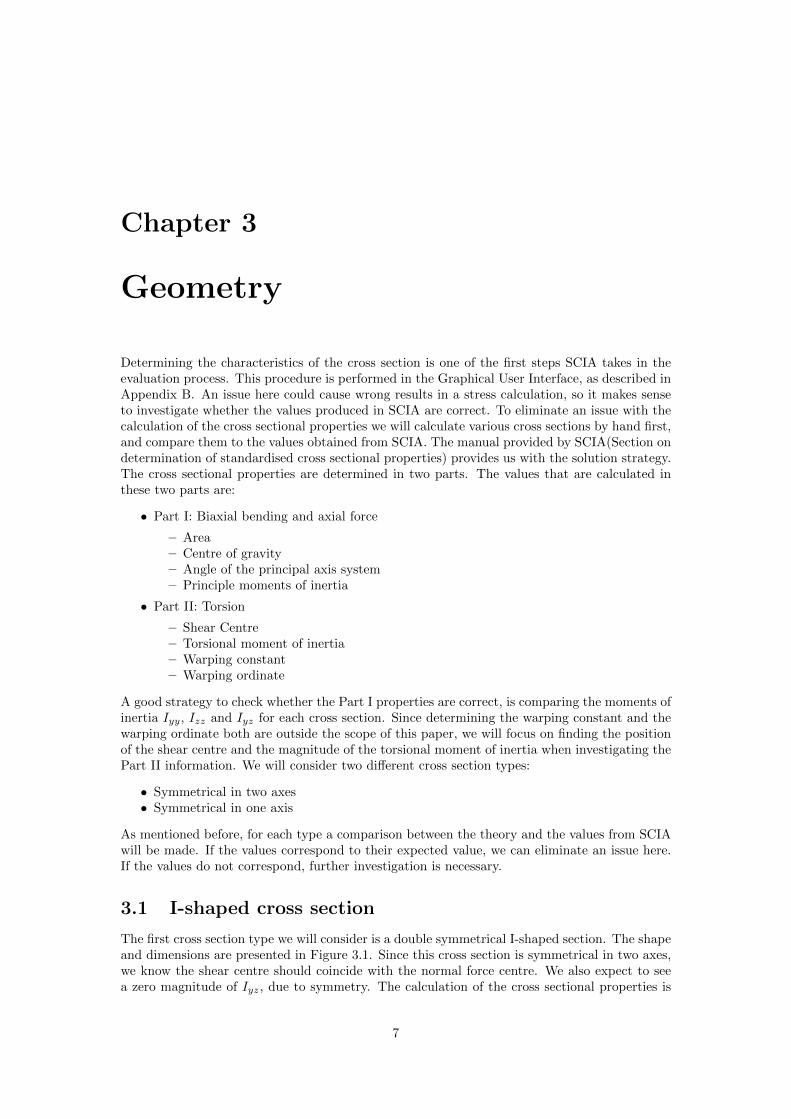
Determining the characteristics of the cross section is one of the first steps SCIA takes in theevaluation process. This procedure is performed in the Graphical User Interface, as described inAppendix B. An issue here could cause wrong results in a stress calculation, so it makes senseto investigate whether the values produced in SCIA are correct. To eliminate an issue with thecalculation of the cross sectional properties we will calculate various cross sections by hand first,and compare them to the values obtained from SCIA. The manual provided by SCIA(Section ondetermination of standardised cross sectional properties) provides us with the solution strategy.The cross sectional properties are determined in two parts. The values that are calculated inthese two parts are:

• Part I: Biaxial bending and axial force

– Area– Centre of gravity– Angle of the principal axis system– Principle moments of inertia

• Part II: Torsion

– Shear Centre– Torsional moment of inertia– Warping constant– Warping ordinate

A good strategy to check whether the Part I properties are correct, is comparing the moments ofinertia Iyy, Izz and Iyz for each cross section. Since determining the warping constant and thewarping ordinate both are outside the scope of this paper, we will focus on finding the positionof the shear centre and the magnitude of the torsional moment of inertia when investigating thePart II information. We will consider two different cross section types:

• Symmetrical in two axes• Symmetrical in one axis

As mentioned before, for each type a comparison between the theory and the values from SCIAwill be made. If the values correspond to their expected value, we can eliminate an issue here.If the values do not correspond, further investigation is necessary.

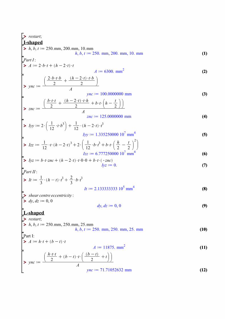
3.1 I-shaped cross section

The first cross section type we will consider is a double symmetrical I-shaped section. The shapeand dimensions are presented in Figure 3.1. Since this cross section is symmetrical in two axes,we know the shear centre should coincide with the normal force centre. We also expect to seea zero magnitude of Iyz, due to symmetry. The calculation of the cross sectional properties is

7

Figure 3.1: I-shaped cross section

performed in Maple, for checking this calculation a reference is made to Appendix C.1. Theresults from SCIA can be observed in Figure 3.2. A comparison between these results is madein table 3.1. As can be observed from this table, the values in SCIA show no discrepancies withthe results from the theory.

Figure 3.2: Cross sectional properties of I-shaped in SCIA

3.2 L-shaped cross section

Now we will consider a cross section that has only one axis of symmetry. The location of theshear centre will therefore not coincide with the normal force centre. The cross section we willdiscuss is L-shaped, and has dimensions as pictured in Figure 3.3. Again the cross section is first

8

Table 3.1: Comparison theory and SCIA for I-shaped cross section

Expectation SCIACentroid (ync,znc) (100mm,125mm) (100mm,125mm)

Area A 6300 mm2 6300 mm2

Moment of inertia y-axis Iyy 6.78 · 107 mm4 6.78 · 107 mm4

Moment of inertia z-axis Izz 1.34 · 107 mm4 1.34 · 107 mm4

Moment of inertia combined Iyz 0 0Torsional moment of inertia It 2.13 · 105 mm4 2.13 · 105 mm4

Eccentricity Shear Centre (dy,dz) (0,0) (0,0)

Figure 3.3: L-shaped cross section

analysed by hand. This hand calculation is reported in the form of a Maple-file in AppendixC.1. The location of the shear centre is determined using the theory that for thin-walled L-shaped cross sections, the shear centre lies on the connection between the two flanges(par. 5.5,Toegepaste Mechanica deel 2, Hartsuijker 2003)[1]. Because the eccentricity of the shear centrewith respect to the normal force centre is given in the principal coordinate system in SCIA, wehave to make an additional calculation. From “Introduction into Continuum Mechanics”[2] weknow the transformation rule for rotating coordinate axes:[

ynewznew

]=

[cos(α) sin(α)− sin(α) cos(α)

]·[yoldzold

](3.1)

Using these facts the theoretical results are obtained. The cross section is also generated inSCIA, the results from that calculation can be seen in Figure 3.4. Now the values can becompared in Table 3.2.

Table 3.2: Comparison between results from the theory and SCIA for an L-shaped cross section

Expectation SCIACentroid (ync,znc) (71.71mm,71.71mm) (71.71mm,71.71mm)

Area A 11875 mm2 11875 mm2

Moment of inertia y-axis Iyy 7.03 · 107 mm4 7.03 · 107 mm4

Moment of inertia z-axis Izz 7.03 · 107 mm4 7.03 · 107 mm4

Moment of inertia combined Iyz −4.16 · 107 mm4 −4.16 · 107 mm4

Torsional moment of inertia It 2.47 · 106 mm4 2.47 · 106 mm4

Eccentricity Shear Centre (dy,dz) (83.74mm,0) (83.97mm,0)

From Table 3.2 it can be concluded that all Part I information is accurate. However, the shearcentre eccentricity is not the same as we have calculated by hand and shows a small discrepancy.The difference in value is 0.23 mm.

9

Figure 3.4: Cross sectional properties of L-shaped in SCIA

3.3 Findings

In this chapter we have analysed two types of cross sections:

• Symmetrical in two axes• Symmetrical in one axis

The values obtained by making a hand calculation have been compared to the result from a cal-culation in SCIA. In section 3.1 we have established that for cross sections that are symmetricalin two axes, the results in SCIA match the theoretical expectation. In section 3.2, an analysiswas made on an L-shaped cross section. This type of cross section is only symmetrical in oneaxis, which means the shear centre does not coincide with the normal force centre. We observedthat the values of most cross sectional properties matched the results in SCIA. However, theshear centre eccentricity reported in SCIA differed from the expectation by 0.23 mm. Furtherinvestigation is necessary to find out where this discrepancy originates.

10

Chapter 4

Boundary Conditions

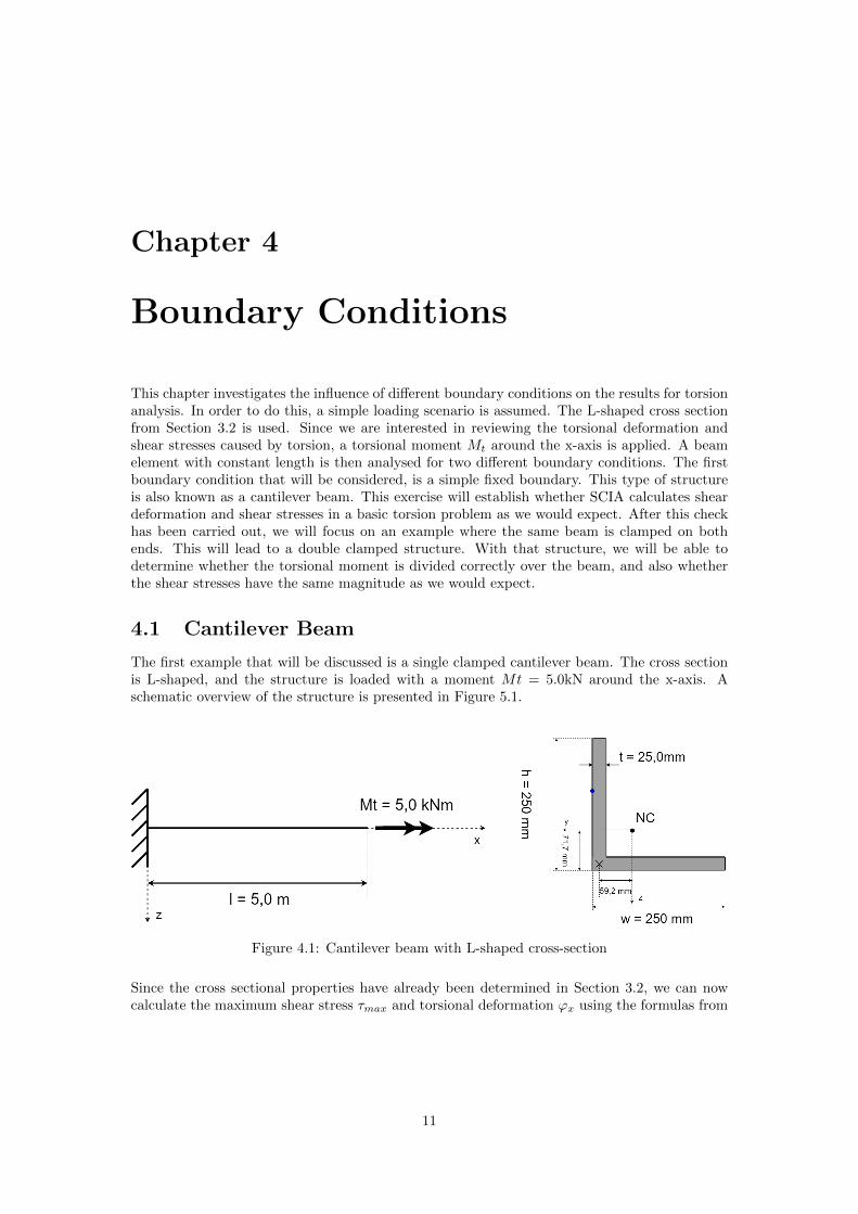
This chapter investigates the influence of different boundary conditions on the results for torsionanalysis. In order to do this, a simple loading scenario is assumed. The L-shaped cross sectionfrom Section 3.2 is used. Since we are interested in reviewing the torsional deformation andshear stresses caused by torsion, a torsional moment Mt around the x-axis is applied. A beamelement with constant length is then analysed for two different boundary conditions. The firstboundary condition that will be considered, is a simple fixed boundary. This type of structureis also known as a cantilever beam. This exercise will establish whether SCIA calculates sheardeformation and shear stresses in a basic torsion problem as we would expect. After this checkhas been carried out, we will focus on an example where the same beam is clamped on bothends. This will lead to a double clamped structure. With that structure, we will be able todetermine whether the torsional moment is divided correctly over the beam, and also whetherthe shear stresses have the same magnitude as we would expect.

4.1 Cantilever Beam

The first example that will be discussed is a single clamped cantilever beam. The cross sectionis L-shaped, and the structure is loaded with a moment Mt = 5.0kN around the x-axis. Aschematic overview of the structure is presented in Figure 5.1.

Figure 4.1: Cantilever beam with L-shaped cross-section

Since the cross sectional properties have already been determined in Section 3.2, we can nowcalculate the maximum shear stress τmax and torsional deformation ϕx using the formulas from

11

Appendix A:

τmax =5.0 · 106Nmm · 12.5mm

0.5 · 2.47 · 106mm4= 50.526N/mm

2

ϕx =5.0 · 106Nmm · 5000mm

8.1 · 104N/mm2 · 2.47 · 106mm4

= 124.75mrad(4.1)

Now the expected values are known, we can focus on the results from SCIA. The geometry andcross section of the structure are imported, and a calculation is performed. The maximum shearstress and torsional deformation according to SCIA are displayed in Figure 4.3 and Figure 4.4respectively.

Figure 4.2: 3D-view of deformed L-shaped cantilever loaded in pure torsion

Figure 4.3: Stress results for L-shaped cantilever loaded in pure torsion

Figure 4.4: Deformation results for L-shaped cantilever loaded in pure torsion

Now we can compare the results. Looking at table 4.1, we observe that the values from SCIAmatch the expected values very well.

Table 4.1: Comparison between theory and SCIA results for L-shaped cantilever

Theory SCIAτmax 50.526 N/mm2 50.526 N/mm2

ϕx 124.75 mrad 124.75 mrad

12

4.2 Double clamped beam

We will consider a beam that is clamped on both ends, similar to the example from the intro-duction. The cross section and the length of the beam are the same as in the previous example.Again the structure will be loaded with a torsional moment only, but we will consider threedifferent positions for the load. The goal is to investigate whether the distribution of the tor-sional moment, and subsequently the shear stresses, are correct. The structure we will analyseis pictured in Figure 4.5.

Figure 4.5: Double clamped cantilever beam with L-shaped cross-section

Expectation

We choose the loading positions the same as in the introduction, so at 1/2, 1/4 and 1/10 ofthe span. These positions are pictured in Figure 4.6. Note that the dotted arrows indicate theposition of the torsional moment, not to be confused with the location of a point load. Themoment distribution due to these loading scenarios can be obtained by using the same solutionstrategy as in the introduction. There we found the torsional moment distribution of a doubleclamped structure is directly proportional to the position of the load. Applying equation (1.3)to this scenario three separate moment distribution graphs can be drawn. These can be foundin Figure 4.7. With this moment distribution the shear stresses can be obtained by filling inequation (A.11).

13

Figure 4.6: Loading positions double clamped cantilever

Figure 4.7: Expected moment distributions

Results in SCIA

The internal moment distribution given by SCIA matches our expectation. The results can beseen in Figure 4.8. The magnitude of the internal forces is correct, but the sign is different.Where we expected to see a positive value, SCIA reports a negative and vice-versa. This is dueto the fact that SCIA can only display the values in the local coordinate system of the crosssection, which is different than the coordinate system we have used in the calculation.

Figure 4.8: Internal moment distribution of double clamped beam in SCIA

The other check that needs to be done is whether this torsional moment leads to the correctshear stresses. Since the shear stresses are linear in Mx, they can be easily computed. The shearstress diagrams from SCIA can be found in Figure 4.9. A comparison between the expectedshear stresses and the results from SCIA is made in table 4.2. Again the sign of the stresses isdifferent than we would expect, but this can be attributed to the coordinate system choice. Themagnitudes of the shear stresses do match our expectation.

Figure 4.9: Shear stress results for double clamped beam in SCIA

14

Table 4.2: Shear stress comparison for double clamped beam

Expectation Shear stress in SCIApart 1 part 2 part 1 part 2

Load midspan 52.26 N/mm2 -52.26 N/mm2 -52.26 N/mm2 52.26 N/mm2

Load 1/4 span 37.89 N/mm2 -12.63 N/mm2 -37.89 N/mm2 12.63 N/mm2

Load 1/10 span 45.47 N/mm2 -5.05 N/mm2 -45.47 N/mm2 5.05 N/mm2

4.3 Findings

From the analysis of a single clamped cantilever beam, we have observed that the values of acalculation in SCIA match the expected values. Therefore we can say that the computationof torsional deformation and shear stresses for a basic torsion problem are correct. From theanalysis of the double clamped beam in section 4.2, we have seen that the distribution ofthe internal torsional moment is correct in SCIA. This was determined using the shear stressdistribution due to a torsional moment applied on different points on the span.

15

Chapter 5

Loading

The next step in the investigation is to consider the loading. Because there are no significantissues when considering geometry and boundary conditions, from now on the focus will beon different loading scenarios. Again we will consider a single clamped beam, which can beconsidered as a simple boundary condition. The same L-shaped cross section is chosen as inprevious examples. We have already established in section 4.1 that for pure torsion, the resultsfor this structure are in line with the theory. To investigate further, this chapter will discussthree different load cases:

• Pure bending with external torque• Point load in normal force centre• Point load in shear centre

5.1 Pure bending

Figure 5.1: Cantilever beam with L-shaped cross-section

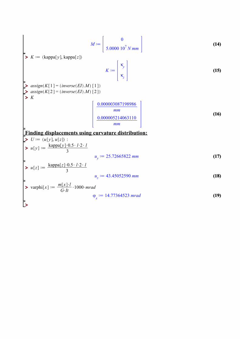
The structure is loaded with a moment Ty around the y-axis at the end of the span. Sincethis cross section is non-symmetrical, the moment of inertia Iyz is non-zero[3]. This meansthat in this example double bending will occur. For clarity reasons, only the main steps of thecalculation will be shown in this section. For the complete calculation, reference is made toAppendix C.2 where a Maple file can be found. The constitutive relation for bending[3] is:[

My

Mz

]=

[EIyy EIyzEIyz EIzz

]·[κyκz

](5.1)

The cross-sectional properties have already been determined in section 3.2. These magnitudescan be found in table 3.2 and the Young’s modulus for steel S235 in table 1.1. Also knowing

16

the moment distribution we obtain the following system:[0

5.0 · 106 Nmm

]= 1012 ·

[14.8 Nmm2 −8.7 Nmm2

−8.7 Nmm2 14.8 Nmm2

]·[κyκz

](5.2)

Elaborating this we obtain the curvatures in y- and z-direction:[κyκz

]=

[3.09 · 10−7

5.21 · 10−7

](5.3)

Now we can calculate the deflections using this curvature distribution. This is done using thetheory from section 8.4 of Hartsuijker[1]. The result is:[

uyuz

]=

[3.859 mm6.518 mm

](5.4)

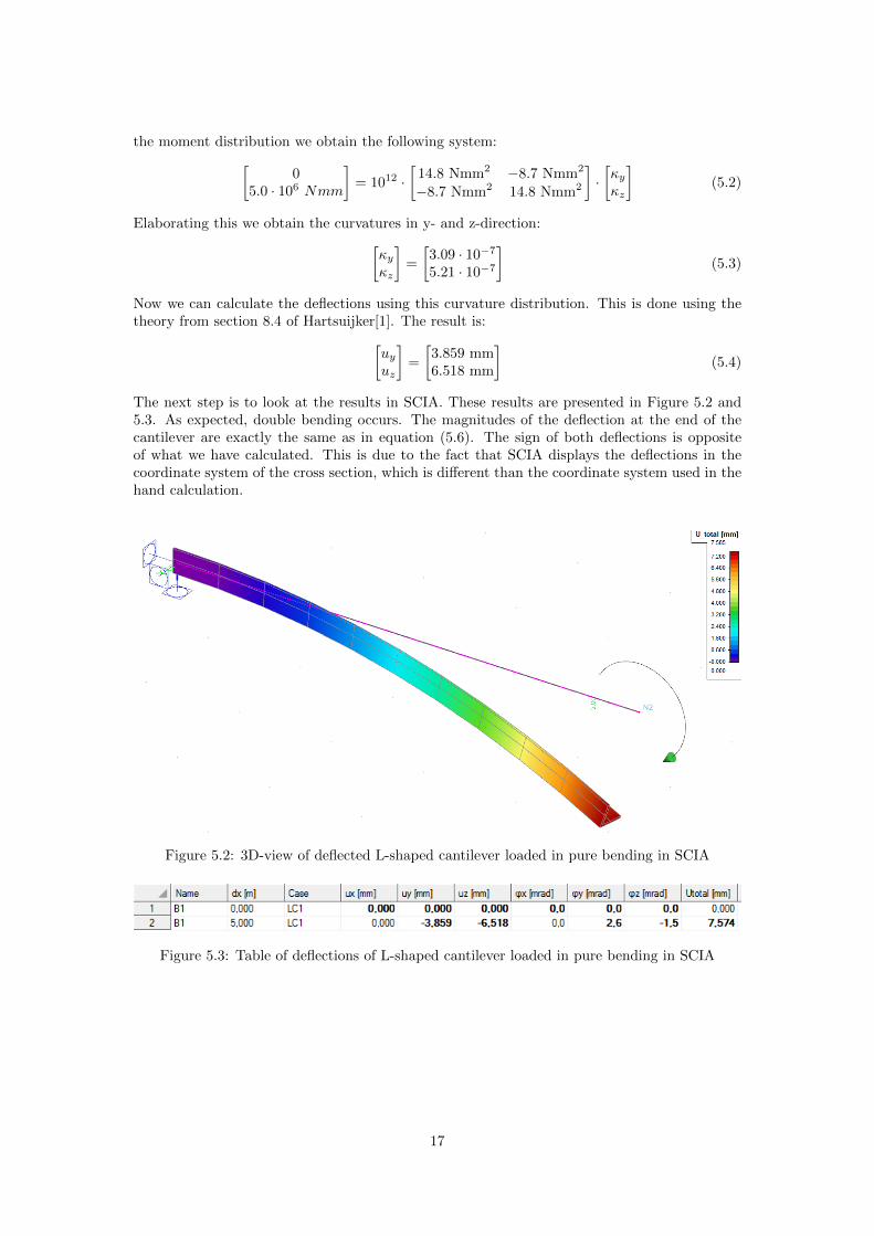
The next step is to look at the results in SCIA. These results are presented in Figure 5.2 and5.3. As expected, double bending occurs. The magnitudes of the deflection at the end of thecantilever are exactly the same as in equation (5.6). The sign of both deflections is oppositeof what we have calculated. This is due to the fact that SCIA displays the deflections in thecoordinate system of the cross section, which is different than the coordinate system used in thehand calculation.

Figure 5.2: 3D-view of deflected L-shaped cantilever loaded in pure bending in SCIA

Figure 5.3: Table of deflections of L-shaped cantilever loaded in pure bending in SCIA

17

5.2 Point load in normal force centre

Figure 5.4: Cantilever beam loaded with a point load in the normal force centre

Table 5.1: Material Properties

Symbol S235Young’s modulus E 210 · 103 N/mm2

Shear modulus G 8.1 · 104 N/mm2

We will consider a cantilever with a L-shaped cross section, as shown in figure 5.4. The materialused for this structure is described in table 5.1. The force F acts in the normal force centre. Weknow from the theory(section 5.5 of Hartsuijker[1]) that in L-shaped cross sections the normalforce centre does not coincide with the shear force centre. Therefore the expectation is that inthis case the force F will not only cause a load in Z-direction, but will also lead to a torsionalmoment. This torsional moment will cause shear stresses and a deformation around the x-axis.The calculation of the expected deformations is performed in two parts. First the deflection dueto bending only is determined. Then the torsional deformation is calculated. Also the expectedmaximum shear stress and internal moment are calculated. The complete calculation procedureis presented in Appendix C.3, but for clarity reasons only the results are presented here. Theexpected deformations in y-,z- and x-direction are:uyuz

ϕx

=

25.73 mm43.45 mm

14.77 mrad

(5.5)

The expected internal forces due to shear centre eccentricity are:[Mx

τmax

]=

[0.592 · 106 Nmm

5.98 N/mm2

](5.6)

The results from SCIA are presented in Figures 5.5, 5.6, 5.7 and 5.8. The value for maximumshear stress was found with the option “consider torsion due to shear centre eccentricity” enabled.Turning this option off, the values in column “τxy/τxs” all reduced to zero.

Now we collect the expectations and the results from SCIA, to compare the magnitudes in table5.2. From the 3D-overview and the deformation results, we observe no rotation around the x-axis. The deflection due to bending in y-direction is correct, but the value in z-direction showssome discrepancy. No torsional moment is reported. And finally, the maximum shear stress thatSCIA reports is also different in value than our expectation.

18

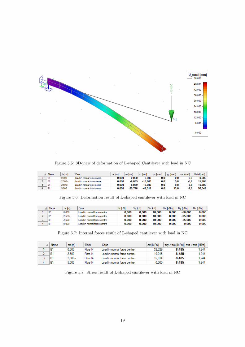
Figure 5.5: 3D-view of deformation of L-shaped Cantilever with load in NC

Figure 5.6: Deformation result of L-shaped cantilever with load in NC

Figure 5.7: Internal forces result of L-shaped cantilever with load in NC

Figure 5.8: Stress result of L-shaped cantilever with load in NC

19

Table 5.2: Comparison between theory and SCIA for L-shaped cantilever with load in NC

Expectation Result in SCIAuy 25.73 mm 25.73 mmuz 43.45 mm 43.51 mmϕx 14.77 mrad 0Mx 0.592·106 Nmm 0τmax 5.98 N/mm2 8.49 N/mm2

5.3 Point load in shear centre

The next loading scenario that will be addressed is a scenario where a point load is appliedat the shear centre of the cross section. According to the theory, no torsion will occur. Thismeans the structure will eflect in y- and z-direction, but no axial deformation will be present.An schematic view of the structure is presented in Figure 5.9.

Figure 5.9: Cantilever beam loaded with a point load in the shear centre

The shear force centre is indicated with a cross in the drawing of the cross section. The locationof this shear centre has already been determined. The eccentricity of this point with respect tothe normal force centre is dy=59.21 mm and dz=59.21 mm. For the calculation process of thislocation, reference is made to Appendix C.1. Because the force has the same magnitude as inthe previous example, and the dimensions of the structure have not changed, the deflections dueto bending moments remain unchanged. The only difference is no rotation around the x-axis isto be expected. The expected deflections are:[

uyuz

]=

[25.73 mm43.45 mm

](5.7)

In SCIA, the same structure is used as in the previous example. However, now the load ischanged to a point load in the shear centre. Because there is no option to do this directly, theeccentricity of the load is inputted manually. The used offsets are dy=59.21 mm and dz=59.21mm. The results from the calculation are presented in Figure 5.10, 5.11, 5.12 and 5.13.

All results are collected in table 5.3. The first observation from this table is that the magnitudeof the deflection in y-direction is according to our expectation. The value for deflection in z-direction however, is not the same. But possibly the biggest discrepancy is that SCIA reportsaxial deformation around the x-axis. This is against our expectation. We also see an internaltorsional moment in the results. The shear stresses that are reported due to “shear centreeccentricity”, again have a value of 8.49 N/mm2.

20

Figure 5.10: 3D-view of deflected L-shaped cantilever loaded in the shear centre in SCIA

Figure 5.11: Table of deflections of L-shaped cantilever loaded in the shear centre in SCIA

Figure 5.12: Internal forces results from SCIA

Figure 5.13: Stress results with option ’consider torsion due to shear centre eccentricity’ enabled

Figure 5.14: Stress results with option ’consider torsion due to shear centre eccentricity’ notenabled

21

Table 5.3: Comparison between theory and SCIA for L-shaped cantilever with load in shearcentre

Expectation Result in SCIAuy 25.73 mm 25.73 mmuz 43.45 mm 43.51 mmϕx 0 mrad 14.8Mx 0 0.592·106 Nmmτmax 0 8.49 N/mm2

5.4 Findings

The analysis of different load scenarios has led to some unexpected results. Although the cal-culations for pure torsion(section 4.1), and pure bending(section 5.1) both are in line with thetheory, it seems the inconsistencies start when bending and torsion are combined. In section5.2 we observe that no torsional deformation and internal torsional moment are calculated. Wealso observe shear stresses that have a different magnitude than we would expect. Although thereported stresses are bigger than expected and thus do not cause an unsafe situation, it raisesquestions on SCIA’s solution strategy.

22

Chapter 6

Conclusion

Recalling from the introduction chapter, several questions were raised regarding a torsion cal-culation in SCIA Engineer. Following from a suspicion that was present regarding torsioncalculations for non-symmetrical cross sections, a structure was considered where shear centreeccentricity played a significant role in the stress calculations. The magnitudes of the shearstresses found in a double clamped structure loaded in bending and torsion were 60% lowerthan the stresses that were expected by using a theoretical approach. In engineering practicesthis discrepancy can lead to very unsafe situations, so the issue should be addressed. This ledto an investigation on different aspects of the torsion calculation, with the ultimate goal toformulate an advice for the software developers. To accomplish this, the area of interest has tobe narrowed down. The investigation described in this paper consists of three sections. Firstthe geometry was checked, then the boundary conditions were considered and lastly differentloading situations were applied. Below, for each of these sections the results are presented andconclusions are drawn.

6.1 Geometry

The first check performed in this paper was whether the determination of cross sectional proper-ties was performed correctly in SCIA. This research was performed in Chapter 3. The questionformulated in the introduction was:

• Does SCIA calculate cross sectional properties in the correct way?

Two types of cross section were investigated, starting with a symmetrical I-shaped section. Thistype of cross section is very common in engineering applications, thus very interesting to con-sider first. The fact that this cross section is symmetrical in two axes, means the shear forcecentre coincides with the normal force center. This left mostly the values for part I of SCIA’sgeometry calculation, the values for bi-axial bending and axial force, to be checked. A com-parison between the values from a hand calculation and the values from SCIA was made, butyielded no discrepancies.

Secondly, an L-shaped cross section was considered. In theory, this type of cross section issymmetrical in only one axis. This means the position of the shear centre does not coincidewith the normal force centre. This fact made this cross section very interesting to investigate,because forces applied in the normal force centre will cause torsion to occur. When the valuesobtained by a hand calculation were compared to the values from SCIA, most magnitudesmatched. Only the determination of the position of the shear centre yielded different results, aspresented in table 6.1:

A discrepancy in the calculation of the shear centre was observed between the theory and SCIA.The difference between the expectation and the observed value was 0.2 mm. However, since this

23

Expectation SCIA DifferenceEccentricity of shear centre inprinciple y-direction

83.74 mm 83.97 mm 0.23 mm

Table 6.1: Comparison between expectation and SCIA

difference is very small, it is not likely to be the cause of the issue described in the introduction.Therefore the choice was made not to investigate this any further.

6.2 Boundary Conditions

The next question that was raised regarded the boundary conditions. This question was:

• Do different boundary conditions influence the torsion results in SCIA?

The checks to formulate an answer to this question were performed in Chapter 4. Here twodifferent boundary conditions were considered for a beam with an L-shaped cross section. Firsta single clamped cantilever beam was analysed. A simple torsional loading scenario was chosen,and the results from a hand calculation were compared to a calculation in SCIA. This test wasperformed to determine whether for a basic torsional problem, the shear stresses and torsionaldeformation is computed according to our expectation. The results from a calculation in SCIAmatched the expected values, so this confirmed there are no issues with the calculation of tor-sional deformation and shear stresses for a basic torsional problem.

Now a double clamped beam is considered. This check determines whether the distribution ofthe internal torsional moment over the beam is correct. Again a non-symmetrical L-shapedcross section was chosen. The structure was analysed for three different positions of the load,similar to the example from the introduction. However, now the load was chosen as a puretorsional moment. The results from a calculation in SCIA showed no discrepancies comparedto the expected values. Therefore we can state that no issues are present in the distribution ofinternal torsional moments.

For both the single-clamped situation and the double-clamped situation, the calculation in SCIAwas correct. Therefore it can be concluded that the boundary conditions have no influence onthe results of torsion calculations in SCIA.

6.3 Loading

The third question that was formulated in the introduction was meant to investigate the influenceof different loading situations on the results for torsion calculations in SCIA. The question was:

• Is the discrepancy between the theory and SCIA influenced by varying the loading?

In Chapter 5, three different loading scenarios were considered for the same structure. Thestructure consisted of a single-clamped L-shaped cantilever. The first check that was performedwas if the deflections of a non-symmetrical cross section loaded in bending only were considered,the values of a hand calculation matched the results from SCIA. The structure was analysedwith a hand calculation first. Comparing the results from this calculation to the results fromSCIA, no differences were found. This means SCIA does use the correct solution strategy fornon-symmetrical cross sections loaded in bending.

The second load scenario that was applied consisted of a point load in the normal force centre.It was previously established that this loading type should cause torsional deformation of thebeam, due to shear centre eccentricity of the cross section. However, observing the results ob-tained from SCIA, no torsional deformation was reported. Also no internal moment around the

24

x-axis was seen, although this was expected. When the results for shear stresses were checked,another inconsistency was found. The shear stress did not have the expected magnitude. Al-though an option is present in the program to “consider torsion due to shear centre eccentricity”,incorrect shear stresses were found. The stresses reported with this option enabled were higherthan expected.

The final loading scenario that was considered, was similar to the previous scenario. However,the point of application of the force was now moved to the shear centre. According to thetheory, this loading situation would cause pure bending of the structure. However, in this caseSCIA does report torsional deformation. Also an internal moment around the x-axis, and shearstresses due to torsion were reported. The difference between the shear stresses with the option“consider torsion due to shear centre eccentricity” enabled and disabled was the same exactvalue as in the load case where the load was applied in the normal force centre.

Combining the knowledge gathered from these three checks, some conclusions can be drawnabout the influence of loading situation on torsion results. The first is that for a beam loadedin pure bending or pure torsion, the values in SCIA match the expectation. However, when aload case is considered where torsion due to shear centre eccentricity is present, the results forthe torsional deformation are not correct. In these cases also the internal torsional moment isnot reported correctly. The option “consider torsion due to shear centre eccentricity” displaysshear stresses in non-symmetrical cross sections loaded in the normal force centre. However, themagnitude of theses stresses is not correct.

25

Chapter 7

Recommendations

Stiffness Matrix

It has been established in this report that the problems regarding torsion in SCIA engineeronly occur when shear centre eccentricity is present. Calculations on pure bending and puretorsion produce correct results when compared to the theory. Only when a load is applied in thenormal force centre of a non-symmetrical cross section, no torsional deformation and internaltorsional moment in the structure are reported. This is not in line with the theory. Given thesesymptoms, an issue may be present in the calculation of beam element stiffness for the stiffnessmatrix. If shear centre eccentricity in this matrix is not implemented correctly or even missingcompletely, this may explain the unexpected results. Perhaps the solution is very simple, andthe problem can be eliminated by adding the shear centre eccentricity to the offset that anelement normal centre line may have with respect to the line drawn in the model.

Shear stresses

The results from the research in this paper indicate that SCIA calculates the shear stresses inpost-processing, which is after the output file from the kernel is imported into the GraphicalUser Interface. In the 3D-stress results section, SCIA gives the option “consider torsion due toshear centre eccentricity”. With this option enabled, shear stress results are displayed. However,the magnitude of these shear stresses differ from their theoretical expectation. This issue waspresented in the introduction of this report, in section 1.2. When the stiffness matrix is corrected,the shear stresses due to torsion will be computed directly from the internal torsional moments.This means the value will be correct, independent of shear centre eccentricity. Therefore thisoption and the underlying code can be removed.

26

Bibliography

[1] Coenraad Hartsuijker, Toegepaste Mechanica - deel 2: spanningen, vervormingen, ver-plaatsingen, Academic Service, Schoonhoven, 2nd edition, 2003.

[2] Hans Welleman, Introduction into Continuum Mechanics, TU Delft, December 2007

[3] Hans Welleman, Lecture notes for Structural Mechanics 4 - Module: Non-symmetrical andinhomogeneous cross sections, TU Delft, April 2017

27

Appendices

28

Appendix A

Torsion Theory

In this paper, structures will be discussed where torsion plays a role. To provide some back-ground on the the theory of torsion, this paragraph is presented to provide the reader with thenecessary explanation of the used formulas.

Coordinate system

First a coordinate system is defined. We will use the coordinate system pictured in Figure A.1.We observe a xyz-coordinate system where the x-axis coincides with the fibres in the normal

Figure A.1: Definition of coordinate Axes

force centre of the beam. This normal force centre, denoted by NC, is defined as “The point ina cross section where the resultant normal force, caused by extension of the element, acts”[1,Chapter 3.1.3, p.69]. This also means it is the point of the cross section where, if a normalforce is applied, no bending moments will occur in the element. Also a shear force centre can bedefined. According to (Hartsuijker, 2003)[Chapter 5.5, p.331]: “If the line of action of the shearforce goes through the point that is called the shear force centre DC, no torsion will occur”.This point is denoted by DC in Figure A.1. In symmetrical cross sections, the shear force centercoincides with the normal force centre. The z-axis is pointed downwards, so positive loads willcause deformations in downward direction. Also rotations have to be described. A rotation ϕx

around the x-axis is defined as a rotation from y to z. A ϕy is defined as a rotation from z tox and a rotation ϕz from x to y. A positive rotation is caused by a positive moment. The signsof the stresses also follow these directions.

Loading types

To introduce the concept of torsion, we start with two simple loading types in 2D. In Figure

29

Figure A.2: 2D-loading types

A.2, two different loading situations are sketched. In the first case, the structure is loaded witha normal force. This will cause deformation of the element, in this case extension. The secondexample is loaded in bending. The loading causes bending moments to occur, which lead tothe structure deforming in a curved shape. For some engineering purposes it will suffice to onlyconsider these loading types for stress and strain calculations. If we expand to 3D however,another loading type arises which needs to be addressed. This loading type is torsion, and isvisualised in Figure A.3. Torsion occurs when an element is loaded with a moment around thebeam axis. This type of loading causes axial deformation, which leads to a rotation of the crosssection.

Figure A.3: Torsion in a beam element

Stress and strain caused by torsion

To analyse stresses and strains caused by torsion, in this paragraph three types of cross sectionsare presented. The first type of cross section that will be discussed is the thin walled circularcross section. The second type is a closed circular cross section. The third type that will bediscussed is a thin walled open cross section. for these three types, the formulas will be presentedfor the calculation of torsional deformation and shear stresses. The theory presented here willbe used throughout the paper, which means this section is meant as a reference. The theorythat is used is extracted from the book on engineering mechanics by Coenraad Hartsuijker[1].For derivations and more information a reference is made to this book. Here only the results ofthese derivations are presented, since proving the formulas is beyond the scope of this paper.

30

Thin walled circular cross section

Figure A.4: Example of thin walled circular cross section

In Figure A.4 an example of a thin walled circular cross section is shown. As presented in(Hartsuijker, 2003)[1] in chapter 6.2 on page 373, the shear stresses for thin walled circular crosssections can be assumed constant over the thickness of the material. The value of this stresscan be computed by equation (A.1).

τ =Mt ·RIp

(A.1)

Here, Mt is the torsional moment present in the cross section, R is the radius of the circle andIp is the polar moment of inertia. This moment of inertia has a value of

Ip = 2πR3t (A.2)

Where R is the radius of the circle and t is the thickness of the material. Subsequently, a crosssection loaded in torsion will undergo torsional deformation. This deformation is defined as arotation around the x-axis, denoted by ϕx. The constitutive relation between torsional momentand deformation is given by

χ =dϕx

dx=

Mt

GIp(A.3)

Where G is the material specific torsion constant, and χ is the contortion of the beam. Thiscontortion value shows large similarities to the ε in case of extension and κ in case of bending.For constant torsional moment, the rotation due to this moment can be computed by

ϕx =Mt · lGIp

(A.4)

Where l is the length of the element.

31

Closed circular cross section

Figure A.5: Example of closed circular cross section

The next step is to expand to a closed circular cross section. An example of this type of crosssection is presented in figure A.5. This type of cross section is thought to be built up out ofmultiple thin-walled sections fitted together. The constitutive relation from equation (A.3) stillholds, but the polar moment of inertia now has a different value, given by (A.5).

Ip =1

2πR4 (A.5)

The assumption of constant stress over the thickness is not valid anymore for this case. Now weobserve a shear stress that is linear in the radius of the circle. This shear stress has a value of:

τ(r) =Mt · rIp

(A.6)

Where r is the distance to the centre line of the circle.

Thin walled open cross sections

An example of a thin walled open cross section is presented in figure A.6. It can be proven that

Figure A.6: Example of thin walled open cross section

for thin walled open cross sections, the constitutive relation for torsion deformation is of theform:

ϕx =Mt · lGIt

(A.7)

where It is now the torsional moment of inertia. This is a different value than the polar momentof inertia we used before, and can be computed by:

It =

n∑i=1

1

3hit

3i (A.8)

32

Which is the summation of the torsional moments of inertia of every strip element out of whichthe cross section is built up. For each of these strip elements, h is the height and t is thethickness of the element. For the cross section of the example in Figure A.6, this leads to atorsional moment of inertia of

It =1

3ht3 +

2

3bt3 (A.9)

For thin walled open cross sections, the shear stresses are proportional to the distance to thecentre line of the elements. The formula to calculate the stresses is:

τ =Mt · sc

12It

(A.10)

Where sc is the distance to the centre line of the element. For stress calculations, we are mostlyinterested in the maximum shear stress. From this theory, we now know the maximum shearstress occurs when sc = t

2 . With this knowledge we can write an expression for the maximumshear stress:

τmax =Mt · tIt

(A.11)

33

Appendix B

Framework Analysis

For the automated calculation and analysis of structures a lot of different software is availableon the market. The SCIA Engineer software package that is being used throughout this paper isa ’Framework Analysis’ program. It also incorporates finite element technology. To understandhow the program works, it is important to look at all the individual steps the software takes toget from an inputted structure to a complete structural analysis. To illustrate how this is done,in this chapter an overview will be presented of the key steps to get from input to a calculation,and ultimately to a usable result. Because this would get very complicated very fast if we woulddiscuss every single aspect of the process, we will use a simplification of reality. Although thismeans we will not discuss some processes in the program, it will illustrate the operation of thesoftware in a clean and simple manner.

B.1 Overview

A flowchart of the steps necessary to get to a calculation is pictured in Figure B.1. The processcan be roughly divided into three steps. The first step is the generation of an input file for thekernel. In this file, for each element in the framework, a stiffness matrix is generated. Alsothe material properties are imported from the GUI and the loads are processed. The secondstep is the actual calculation. This is done in the ’kernel’, which is the mathematical heartof the software. Here a large K-matrix is generated, in which the stiffness matrices for all theindividual frame elements are assembled. This leads to a large system of equations, that canbe solved for all the deflections. These deflections are then substituted back into the individualstiffness relations, to obtain the internal forces. The third an last step, is importing these valuesin the output file back into the graphical user interface. During this final step the unity checksare performed and also the stresses in the cross sections can be computed. Each of the stepswill be further elaborated in the following paragraphs.

B.2 Generation of input file

The first step in any frame analysis software is the generation of the input file. The structurethat has been created by the user has to be converted into a model that can be evaluated. Thismeans the structure in the graphical interface first has to be divided into individual elements.To illustrate how this is done, we will consider a simple portal structure as pictured in FigureB.2 The elements are have a rigid connection in node B and C. The structure is loaded witha unit moment ’T’ in node B. The two supports in A and D are hinges, and a third supportin C is added to prevent swaying of the structure. This means all the nodes can only rotate,no lateral displacements are possible. To start the modelling of this structure, we first dividethe structure into three individual, static determinate beams. The model becomes Figure B.3.Then we consider the beam between A and B. We are looking for a system of equations in the

34

Figure B.1: Schematic overview of framework software

35

Figure B.2: Portal Structure

form:

m = K ·ϕ→[MA

MB

]=

[kaa kabkba kbb

]·[ϕA

ϕB

](B.1)

Where m is the load vector, ϕ is the displacement vector and K is the flexibility matrix. Inwords this equation means we have to find relations between the moments in the nodes and therotations of the elements connected to the nodes. These can be found by solving the fourthorder differential equation for bending. The solution for this simple load case is already knownand can be found in the ’forget-me-nots’. To simplify things, we will first set ϕA to 0, whilesetting ϕB to 1. This leaves us with two equations.[

MA

MB

]=

[kaa kabkba kbb

]·[01

]→[MA

MB

]=

[kabkbb

](B.2)

This means if we find the moments in A and B due to a unit rotation in B, we obtain the valuesof kab and kbb. The rotation in B due to a moment in B can be found in Figure B.4. However,we are interested in the moment due to a rotation. This relation can be obtained by rewritingthe expression, knowing that ϕB has a value of 1:

ϕB =MB · l4EI

= 1→MB =4EI

l→ kbb =

4EI

l(B.3)

We also know from the ’forget-me-nots’, that in this type of loading situation the moment inthe support in A will be half the moment excited at B. This means:

MA =MB

2=

2EI

l→ kab =

2EI

l(B.4)

36

divided.png

Figure B.3: Portal Structure divided into individual elements

Filling in the values for kab and kbb, we obtain the system:[MA

MB

]=

[kaa

2EIl

kba4EIl

]·[ϕA

ϕB

](B.5)

Now we set the value of ϕA to 1 and the value of ϕB to 0. In a similar manner, we obtain thevalues for kaa and kba. The final system of equations for the first element becomes:[

MA

MB

]=

[4EIl

2EIl

2EIl

4EIl

]·[ϕA

ϕB

](B.6)

The process described above is repeated for all three elements in the framework. This leads tothree individual flexibility relations; one for each element. In this case the flexibility matricesare identical, because the lengths and stiffnesses of all the elements are the same. The relationsare: [

MA

MB

]=

[4EIl

2EIl

2EIl

4EIl

]·[ϕA

ϕB

][MB

MC

]=

[4EIl

2EIl

2EIl

4EIl

]·[ϕB

ϕC

][MC

MD

]=

[4EIl

2EIl

2EIl

4EIl

]·[ϕC

ϕD

] (B.7)

In SCIA, this is the end of the first step. Loads, stiffness and length of all the elements arewritten to an input file for the kernel. In reality, a lot more data is reported than we havedemonstrated above. For example distributed loads are taken into account and torsion stiffnessand deformation is added. Also the model in SCIA is 3D, whereas our model only has twodimensions. All these features are implemented in the input file, but the overall process is thesame as we have done.

B.3 The Kernel

The previous paragraph has presented how a mathematical model is generated for a frameworkstructure. Now the input file has been generated, the actual calculation can be made. This is

37

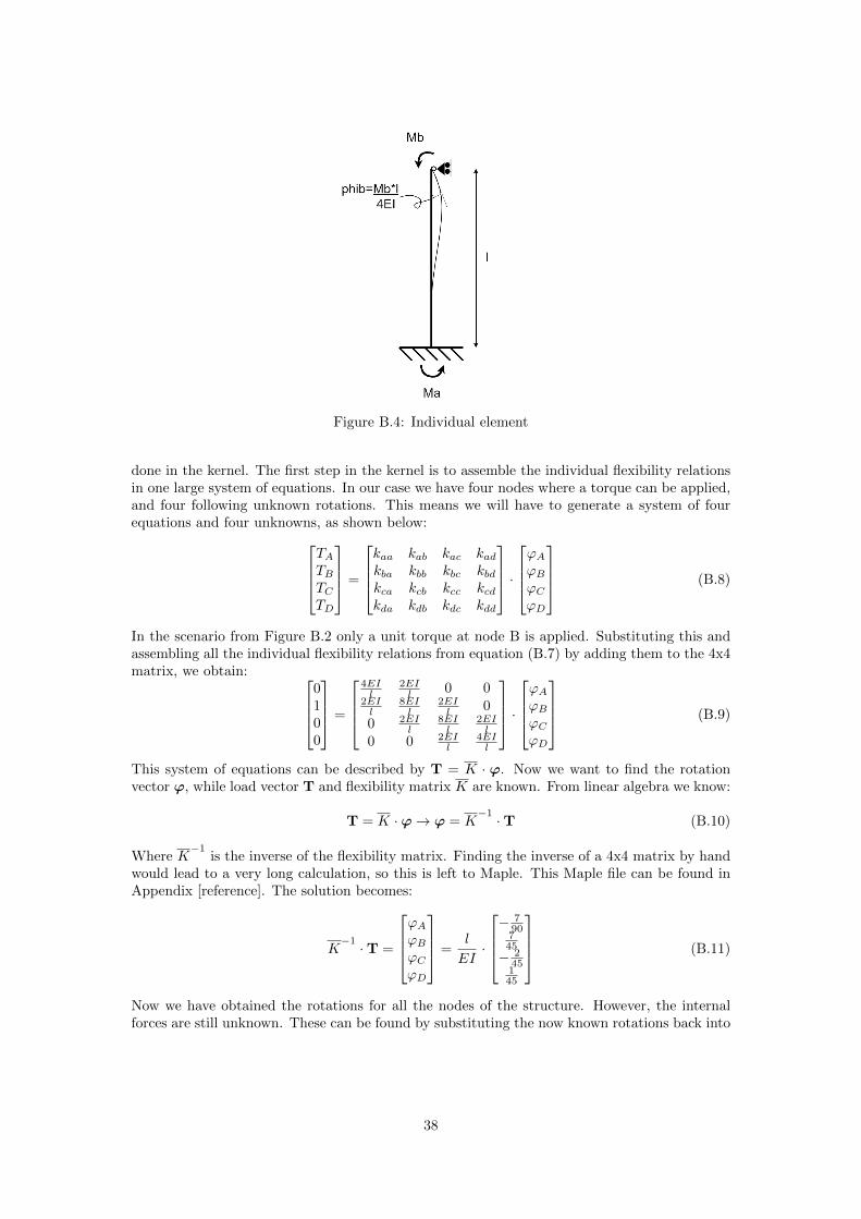
Figure B.4: Individual element

done in the kernel. The first step in the kernel is to assemble the individual flexibility relationsin one large system of equations. In our case we have four nodes where a torque can be applied,and four following unknown rotations. This means we will have to generate a system of fourequations and four unknowns, as shown below:

TATBTCTD

=

kaa kab kac kadkba kbb kbc kbdkca kcb kcc kcdkda kdb kdc kdd

·ϕA

ϕB

ϕC

ϕD

(B.8)

In the scenario from Figure B.2 only a unit torque at node B is applied. Substituting this andassembling all the individual flexibility relations from equation (B.7) by adding them to the 4x4matrix, we obtain:

0100

=

4EIl

2EIl 0 0

2EIl

8EIl

2EIl 0

0 2EIl

8EIl

2EIl

0 0 2EIl

4EIl

·ϕA

ϕB

ϕC

ϕD

(B.9)

This system of equations can be described by T = K · ϕ. Now we want to find the rotationvector ϕ, while load vector T and flexibility matrix K are known. From linear algebra we know:

T = K ·ϕ→ ϕ = K−1 ·T (B.10)

Where K−1

is the inverse of the flexibility matrix. Finding the inverse of a 4x4 matrix by handwould lead to a very long calculation, so this is left to Maple. This Maple file can be found inAppendix [reference]. The solution becomes:

K−1 ·T =

ϕA

ϕB

ϕC

ϕD

=l

EI·

− 7

90745− 2

45145

(B.11)

Now we have obtained the rotations for all the nodes of the structure. However, the internalforces are still unknown. These can be found by substituting the now known rotations back into

38

the individual flexibility relations of the elements. This is done below:[MA

MB

]=

[4EIl

2EIl

2EIl

4EIl

]·[− 7·l

90EI7·l

45EI

]=

[0715

][MB

MC

]=

[4EIl

2EIl

2EIl

4EIl

]·[

7·l45EI

− 2·l45EI

]=

[815215

][MC

MD

]=

[4EIl

2EIl

2EIl

4EIl

]·[− 2·l

45EIl

45EI

]=

[− 2

150

] (B.12)

What stands out is the fact the two values for MB are not the same. This means the value ofthe moment in the beam is different on each side of the node. This is due to the fact that theload is applied in B. The combined value of the two internal moments equals 7

15 + 815 = 1 This

moment counteracts the applied torque, which also has a value of 1. This means the sum ofmoments on that node equals 0, which is what we would expect. Now all the variables we neededto determine are known. This is the end of the second step in SCIA. What we have done aboveis again a simplification of what happens in reality. The matrix and vectors will be much larger,but also other things may vary. Adding a fixed support for instance makes the applied torque inthat node a variable, while keeping the rotation fixed at 0. However, the general concept of howan input file is converted into usable results remains unchanged. All the results are ultimatelycollected in an output file.

B.4 GUI

Now the main calculation is done, the third and final step is to display the results in theGraphical User Interface, the GUI. During this step, some additional calculations are performedon the results. To check whether a structure doesn’t exceed the maximum allowed deflectionsor stresses, unity checks are performed. Safety factors and load combinations are collected andreported. The maximum stresses in the cross sections can also be computed, now the internalforces in the elements are known. SCIA also has the ability to draw the structure in deformedstate, even in 3D. All this is done with the values obtained by the calculation in the Kernel.

Maple Files for framework analysis of simple portal struc-ture

39

Figure B.5: 1

Figure B.6: 2

40

Figure B.7: 3

41

Appendix C

Maple Files

C.1 Cross sectional properties

42

> >

(6)(6)

(7)(7)

> >

> >

> >

(5)(5)

(4)(4)

> >

> >

> >

> >

> >

> >

(3)(3)

(10)(10)

> >

(2)(2)

(8)(8)

(12)(12)

(9)(9)

> >

(11)(11)

> >

> >

> >

(1)(1)

I-shaped

L-shaped

Part I:

> >

(16)(16)

(18)(18)

> >

(19)(19)

(20)(20)

(14)(14)

(13)(13)

> >

(15)(15)

> >

> >

> >

(17)(17)

> >

> >

> >

Shear centre eccentricity in local coordinate system:

Shear centre eccentricity in principal coordinate system:

C.2 L-shaped cross section loaded in pure bending

45

> >

(10)(10)

> >

> >

(6)(6)

> >

> >

> >

(11)(11)

> >

> >

(8)(8)

> >

(3)(3)

> >

> >

> >

(4)(4)

(2)(2)

(9)(9)

> >

> >

(5)(5)

(7)(7)

(1)(1)

> >

Loading:

Cross sectional properties:

> >

(13)(13)

> >

(12)(12)

> >

> > Finding displacements using curvature distribution:

C.3 L-shaped cross section loaded in normal force centre

48

(14)(14)

> >

(9)(9)

> >

(1)(1)

> >

> >

(8)(8)

(7)(7)> >

> >

> >

> >

> >

(6)(6)

(13)(13)

> >

> >

(3)(3)

(5)(5)

> >

(12)(12)

> >

> >

(2)(2)

(4)(4)> >

(11)(11)

> >

> >

(10)(10)

Input:

Loading:

Cross sectional properties:

(14)(14)

> >

> >

(16)(16)

> >

(17)(17)

(19)(19)

> >

> >

> >

> >

(15)(15)

> >

> >

(18)(18)

Finding displacements using curvature distribution: