Topology Optimization and Analysis of Thermal and ...
101
Dissertations and Theses 7-2020 Topology Optimization and Analysis of Thermal and Mechanical Topology Optimization and Analysis of Thermal and Mechanical Metamaterials Metamaterials Lee Alacoque Follow this and additional works at: https://commons.erau.edu/edt Part of the Aerospace Engineering Commons Scholarly Commons Citation Scholarly Commons Citation Alacoque, Lee, "Topology Optimization and Analysis of Thermal and Mechanical Metamaterials" (2020). Dissertations and Theses. 530. https://commons.erau.edu/edt/530 This Thesis - Open Access is brought to you for free and open access by Scholarly Commons. It has been accepted for inclusion in Dissertations and Theses by an authorized administrator of Scholarly Commons. For more information, please contact [email protected].
Transcript of Topology Optimization and Analysis of Thermal and ...

Dissertations and Theses
7-2020
Topology Optimization and Analysis of Thermal and Mechanical Topology Optimization and Analysis of Thermal and Mechanical
Metamaterials Metamaterials
Lee Alacoque
Follow this and additional works at: https://commons.erau.edu/edt
Part of the Aerospace Engineering Commons
Scholarly Commons Citation Scholarly Commons Citation Alacoque, Lee, "Topology Optimization and Analysis of Thermal and Mechanical Metamaterials" (2020). Dissertations and Theses. 530. https://commons.erau.edu/edt/530
This Thesis - Open Access is brought to you for free and open access by Scholarly Commons. It has been accepted for inclusion in Dissertations and Theses by an authorized administrator of Scholarly Commons. For more information, please contact [email protected].

TOPOLOGY OPTIMIZATION AND ANALYSIS OF THERMAL AND
MECHANICAL METAMATERIALS
By
Lee Alacoque
A Thesis Submitted to the Faculty of Embry-Riddle Aeronautical University
In Partial Fulfillment of the Requirements for the Degree of
Master of Science in Aerospace Engineering
July 2020
Embry-Riddle Aeronautical University
Daytona Beach, Florida
ii
TOPOLOGY OPTIMIZATION AND ANALYSIS OF THERMAL AND
MECHANICAL METAMATERIALS
By
Lee Alacoque
This Thesis was prepared under the direction of the candidate’s Thesis Committee Chair,
Dr. Ali Tamijani, Department of Aerospace Engineering, and has been approved by the
members of the Thesis Committee. It was submitted to the Office of the Senior Vice
President for Academic Affairs and Provost, and was accepted in the partial fulfillment of
the requirements for the Degree of Master of Science in Aerospace Engineering.
THESIS COMMITTEE
Chairman, Dr. Ali Tamijani
Member, Dr. Daewon Kim
Member, Dr. Marwan Al-Haik
Graduate Program Coordinator,
Dr. Magdy Attia
Date
Dean of the College of Engineering,
Dr. Maj Mirmirani
Date
Associate Provost of Academic Support,
Dr. Christopher Grant
Date

iii
ACKNOWLEDGEMENTS
Firstly, I would like to thank my advisor, Dr. Ali Tamijani, for guiding, supporting,
and motivating me to always perform my best. I have learned an incredible amount
during the challenges of the past two years, far more than I could have done on my own.
To the committee members Dr. Al-Haik and Dr. Kim, thank you for the extremely
helpful suggestions, advice, and assistance with setting up the experimental portions of
the work.
For all of the insightful discussions and ideas, thank you to Dr. Ryan Watkins of
NASA Jet Propulsion Laboratory. Your inputs have significantly shaped the course of
this research and the final results would not have been the same without you.
I would also like to thank my co-researchers Kaveh Gharibi, Rossana Fernandes,
Chitrang Patel, Patricia Velasco, and Zhichao Wang whose collaborations and assistance
considerably helped the progression of my own thesis work.
Lastly, I would like to thank my parents for their continued support throughout my
life, which has allowed me to be where I am today.

iv
ABSTRACT
To take advantage of multi-material additive manufacturing technology using mixtures of
metal alloys, a topology optimization framework is developed to synthesize high-strength
spatially periodic metamaterials possessing unique thermoelastic properties. A thermal
and mechanical stress analysis formulation based on homogenization theory is developed
and is used in a regional scaled aggregation stress constraint method, and a method of
worst-case stress minimization is also included to efficiently address load uncertainty. It
is shown that the two stress-based techniques lead to thermal expansion properties that
are highly sensitive to small changes in material distribution and composition. To resolve
this issue, a uniform manufacturing uncertainty method is utilized which considers
variations in both geometry and material mixture. Test cases of high stiffness, zero
thermal expansion, and negative thermal expansion microstructures are generated, and
the stress-based and manufacturing uncertainty methods are applied to demonstrate how
the techniques alter the optimal designs. Large reductions in stress are achieved while
maintaining robust strength and thermal expansion properties.
An extensive analysis is also performed on structures made from two-dimensional lattice
materials. Numerical homogenization, finite element analysis, analytical methods, and
experiments are used to investigate properties such as stiffness, yield strength, and
buckling strength, leading to insights on the number of cells that must be included for
optimal mechanical properties and for homogenization theory to be valid, how failure
modes are influenced by relative density, and how the lattice unit cell can be used to
build macrostructures with performance superior to structures generated by conventional
topology optimization.

v
TABLE OF CONTENTS
ACKNOWLEDGEMENTS........................................................................................... iii
ABSTRACT................................................................................................................... iv
LIST OF FIGURES........................................................................................................ vii
LIST OF TABLES......................................................................................................... x
SYMBOLS..................................................................................................................... xi
ABBREVIATIONS........................................................................................................ xv
1. Introduction................................................................................................................ 1
2. Metamaterial Topology Optimization: Methodology................................................ 9
2.1. Homogenization Theory and Finite Element Formulation............................... 9
2.2. Filtering of Design Variables............................................................................ 13
2.3. Material Property Interpolation Models............................................................ 14
2.4. Microstructure Thermoelastic Stress Analysis.................................................. 16
2.5. Failure Constraints............................................................................................ 18
2.6. Load Uncertainty............................................................................................... 20
2.7. Manufacturing Uncertainty............................................................................... 22
2.8. Sensitivity Analysis........................................................................................... 23
3. Metamaterial Topology Optimization: Numerical Examples.................................... 27
3.1. Thermoelastic Stress Analysis Verification...................................................... 29
3.2. Maximum Orthotropic Stiffness Single-Material Microstructure..................... 30
3.3. Maximum Isotropic Stiffness, Zero Thermal Expansion Microstructure......... 32
3.4. Negative Thermal Expansion Microstructure................................................... 39
4. Lattice Structures: Numerical Analysis..................................................................... 44
4.1. Unit Cell Geometry........................................................................................... 44
4.2. Homogenization of Unit Cell Properties........................................................... 45
4.3. Analytical Equations......................................................................................... 48
4.4. Effect of the Number of Cells on Young’s Modulus........................................ 49
4.5. Effect of Relative Density on Young’s Modulus.............................................. 54
4.6. Effect of the Number of Cells on Buckling Load............................................. 56
4.7. Effect of Relative Density on Buckling Load and Failure Mode..................... 57
5. Lattice Structures: Experimental Analysis................................................................. 59
5.1. Additive Manufacturing Process and Material Properties................................ 59
5.2. Simple Lattice Structures.................................................................................. 61
5.3. Spatially Varying Lattice Structures: Cantilever Beam.................................... 67
5.4. Spatially Varying Lattice Structures: Three-Point Bending............................. 72

vi
6. Conclusions................................................................................................................ 77
REFERENCES............................................................................................................... 80
vii
LIST OF FIGURES
Figure Page
3.1 Color representation of the composition variable x2 for plots of designs made
from Invar 36, stainless steel 304L, and their mixtures...................................... 28
3.2 Thermal and mechanical stress computed using the presented
homogenization-based formulation compared to a standard mechanics
analysis in ANSYS. (a) The cell geometry and composition; (b) the
microscopic stress computed using the homogenization-based formula; and
(c) the stress computed using ANSYS showing a single cell at the center of
the macrostructure..............................................................................................
29
3.3 Results of optimization problems (a), (b), and (c). Density and composition
shown in column (i); polar plots of homogenized Young’s modulus EH (GPa)
shown in column (ii); von Mises failure index F shown in column (iii); and
worst-case von Mises failure index Fs (× 10-8) shown in column (iv)............ 31
3.4 Results of optimization problems (d), (e), (f), and (g). Density and
composition shown in column (i); polar plots of homogenized Young’s
modulus EH (GPa) shown in column (ii); von Mises failure index F shown in
column (iii); and worst-case von Mises failure index Fs (× 10-8) shown in
column (iv)......................................................................................................... 33
3.5 The upper bounds of bulk modulus (Pa) for zero thermal expansion isotropic
microstructures of every possible volume fraction. The highest values occur
for large volume fractions of Invar, the weaker of the two materials................ 34
3.6 Uniform manufacturing uncertainties of designs (f) and (g) with their
homogenized thermal expansions and worst-case stress distributions............... 38
3.7 Results of optimization problems (h), (i), (j), and (k). Density and
composition shown in column (i); polar plots of homogenized Young’s
Modulus EH (GPa) shown in column (ii); von Mises failure index F shown in
column (iii); and worst-case von Mises failure index Fs (× 10-7) shown in
column (iv)......................................................................................................... 40
3.8 Uniform manufacturing uncertainties of designs (j) and (k) with their
homogenized thermal expansions and worst-case stress distributions............... 43
4.1 Geometry of the unit cell, where L the side length of the square domain and t is the wall thickness............................................................................................ 44
4.2 Illustration of how more cells are added to the lattice structure while
maintaining constant relative density and domain shape................................... 45

viii
Figure Page
4.3 Relative density of the FE mesh and homogenized value of Young’s modulus
in the 1 direction versus the number of elements along the domain side
length................................................................................................................... 46
4.4 The normalized homogenized Young’s modulus E1H/Es of the unit cell
plotted as a function of direction in polar coordinates for several different
relative densities................................................................................................. 47
4.5 Effective Young’s modulus in the 1 direction computed by FEA versus the
out-of-plane length of the cell. The homogenized value computed by the 3D
code is shown by the solid black horizontal line................................................ 51
4.6 Three-dimensional end effects in a finite element simulation von Mises stress
plot. As the out-of-plane cell length increases, the contribution of the end
effects to the effective properties of the cell becomes negligible and the
effective property approaches the homogenized value....................................... 52
4.7 Effective Young’s modulus in the 1 direction versus the number of cells
making up the structure, where the homogenized value is shown by the solid
black horizontal line........................................................................................... 53
4.8 Normalized effective Young’s moduli when loaded at a 45 degree angle for
30%, 50%, and 70% relative densities versus the number of cells in the
structure. The normalized homogenized values of each density are shown by
the solid black horizontal line............................................................................. 54
4.9 Young’s modulus versus relative density for a 30% relative density lattice...... 55
4.10 Von Mises stress contour plot and deformation of a lattice cell under a
compression displacement in the vertical direction. The deformation of the
horizontal member contributes to the effective stiffness of the lattice............... 55
4.11 Effective buckling stress and mode shapes of a 30% relative density lattice
versus number of cells in the structure............................................................... 56
4.12 Effective failure stresses versus relative density for an 8x8 lattice structure.
The intersection of the buckling stress curve and yield stress curve represents
the critical density............................................................................................... 57
5.1 Lattice structures printed by the MJF process. 30%, 40%, 50%, and 60%
relative densities from left to right..................................................................... 62
ix
Figure Page
5.2 Effective stress-strain curves from compression tests on 8x8 lattice structures
of relative densities 30%, 40%, 50%, and 60%.................................................. 63
5.3 DIC images showing von Mises strain before and after buckling has occurred.
(a) 30% relative density, which fails by purely elastic buckling, before
buckling and (b) after buckling. (c) 60% relative density, which experiences
material yielding before collapse, before buckling and (d) after
buckling.............................................................................................................. 64
5.4 Nonlinear finite element analysis results compared to experimental results for
8x8 lattice structures of relative density (a) 30%, (b) 40%, (c) 50%, and (d)
60%..................................................................................................................... 65
5.5 Optimized cantilever beam test specimen as printed by MJF............................ 68
5.6 Failure of the optimized lattice cantilever beam................................................ 68
5.7 Force-displacement curve measured during the test of the optimized beam
compared to the slope computed using linear FEA on the three-dimensional
test specimen CAD model.................................................................................. 69
5.8 (a) Von Mises strain results from DIC at a load of 500 N, (b) FEA results at
the same load with color scale values matched as closely as possible to the
DIC results, and (c) the first buckling mode shape............................................ 71
5.9 Three-point bending test specimens as printed by MJF and after testing to
failure. (a) SIMP, (b) triangular lattice (Case 1), (c) triangular lattice (Case
2)......................................................................................................................... 74
5.10 Three-point bending tests. (a) Force per unit frontal surface area versus
crosshead displacement at the point of load application, (b) the SIMP
specimen immediately before complete failure at 8.8 mm of crosshead
displacement, (c) the triangular lattice structure at 7.1 mm of crosshead
displacement after a local failure occurred in one small strut (circled), (d) the
triangular lattice structure at 10.2 mm of crosshead displacement after a local
buckling failure had occurred, (e) the filled triangular lattice structure at 8
mm of crosshead displacement after an initial local buckling failure had
occurred, (f) the filled triangular lattice structure at 9.2 mm of crosshead
displacement after the local failure of two small struts (circled)....................... 76

x
LIST OF TABLES
Table Page
2.1 Material property interpolation functions……………………………………… 16
3.1 Material properties of stainless steel 304L and Invar 36……………………..... 27
5.1 Measured material properties of HP 3D High Reusability PA 12……………... 61
5.2 Lattice wall thickness measurements [mm]…………………………………… 62
5.3 Comparison of Young’s moduli [MPa]………………………………………... 67
5.4 Comparison of effective buckling stress [MPa]……………………………….. 67
5.5 Linear specific stiffness of three-point bending designs with P = 1 kN……….. 73
xi
SYMBOLS
𝑨 Amplification matrix
𝐴 Area
𝜶 Coefficients of thermal expansion
𝜶𝐻 Homogenized coefficients of thermal expansion
𝑩 Strain-displacement matrix
𝜷 Coefficients of thermal stress
𝛽 Projection filter intensity
𝜷𝐻 Homogenized coefficients of thermal stress
𝑪 Stiffness matrix
𝑪𝐻 Homogenized stiffness matrix
𝝌 Fluctuating mechanical displacement
Δ𝑇 Change in temperature
𝛿 Displacement
𝐸 Young’s modulus
𝐸𝐻 Homogenized Young’s modulus
𝐸∗ Effective Young’s modulus
𝐸𝑠 Solid material Young’s modulus
𝜖 Micro-scale to macro-scale size ratio
𝜺 Strain
𝜺0 Unit macroscopic average strain
�̅� Applied macroscopic average strain
𝜺∗ Fluctuating mechanical strain
xii
𝜺𝛼 Thermal strain
𝜂 Projection filter inflection point parameter
𝜂𝑃 Interpolation function for property 𝑃
F Failure index
FPN Failure index p-norm aggregation
Fs Worst-case failure index
FsPN Worst-case failure index p-norm aggregation
𝐅m Mechanical force vector
𝐅th Thermal force vector
𝚪 Thermal displacement
𝑰 Identity matrix
𝑲 Global stiffness matrix
𝒌𝑒 Element stiffness matrix
𝐿 Length
Λ Cell size
𝝀 Adjoint vector
𝑁 Number of elements
𝑁𝑚 Number of stress groups
𝑛 Buckling end constraint factor
𝜈 Poisson’s ratio
𝑃 Applied force
𝑝 P-norm function parameter

xiii
𝜋 The number pi
𝑞𝑃 RAMP interpolation penalty parameter for property 𝑃
𝑅 Reaction force
𝑟𝑚𝑖𝑛 Density filter radius
𝜌∗ Effective density
𝜌𝑠 Solid material density
𝑠 Stress adaptive scale factor
𝑠𝑣𝑀 Worst-case von Mises stress
𝑠𝑣𝑀𝑟 Relaxed worst-case von Mises stress
𝑺𝐻 Homogenized compliance matrix
𝝈 Stress
�̅� Applied macroscopic average stress
𝜎𝑣𝑀 Von Mises stress
𝜎𝑣𝑀𝑟 Relaxed von Mises stress
𝜎𝑎 Allowable stress
𝜎𝑏𝑢𝑐𝑘𝑙𝑖𝑛𝑔∗ Effective buckling stress
𝜎𝑦 Yield stress
𝜎𝑦∗ Effective yield stress
𝜎𝑦𝑠 Solid material yield stress
𝜎𝑢 Solid material ultimate stress
𝑻 Transformation matrix
𝑡 Wall thickness

xiv
𝜃 Rotation angle
𝒖 Displacement field
𝑣 Virtual displacement
𝑉 Volume
𝑉𝑓 Volume fraction or relative density
𝑥 Design variables, macroscopic coordinates
�̃� Density filtered design variables
�̅� Projection filtered design variables
�̅�𝐸 Eroded design variables
�̅�𝐷 Dilated design variables
𝑌 Microscopic domain
𝑦 Microscopic coordinates
xv
ABBREVIATIONS
2D Two-Dimensional
3D Three-Dimensional
ABS Acrylonitrile Butadiene Styrene
ANSYS A commercial engineering simulation software
ASTM American Society for Testing and Materials
CAD Computer Aided Design
DIC Digital Image Correlation
FDM Fused Deposition Modeling
FEA Finite Element Analysis
FFF Fused Filament Fabrication
GCMMA Globally Convergent Method of Moving Asymptotes
HP Hewlett-Packard
MJF Multi-Jet Fusion
PA Polyamide
RAMP Rational Approximation of Material Properties
SIMP Solid Isotropic Material with Penalization
SLS Selective Laser Sintering
SS Stainless Steel
TPMS Triply Periodic Minimal Surface
XFEM Extended Finite Element Method

1
1. Introduction
Additive manufacturing technology has recently advanced to the point where highly
complex structures, which were previously impossible to fabricate, are now feasible
designs for creating functional and load-bearing components for use in industries such as
aerospace, automotive, and biomedical. Among these complex new structures are lattice
structures, which are repeating arrangements of small interconnected features often made
up of straight struts connected at their ends. The smallest repeating unit of these
structures is called the unit cell.
Extensive work has already been completed on lattice structures (L. J. Gibson &
Ashby, 1999). Wang and McDowell (2004) analyzed and presented structural equations
for seven different two-dimensional planar lattice cells. They derived analytical
expressions for in-plane mechanical properties, such as initial yielding and elastic
buckling loads, of several cell geometries. Maskery et al. (2018) computationally and
experimentally investigated three different triply periodic minimal surface (TPMS)
structures, which shed light on their mechanical properties and failure mechanisms and
established relationships between their geometries and mechanical properties. Niu et al.
(2018) developed an analytical solution for the effective Young’s modulus of a three
dimensional triangular lattice structure and compared the results to finite element analysis
and experiment.
Taking the concept of a periodic lattice structure a step further, the geometry and
orientation of the unit cell can be spatially varied to create structures with customized
performance characteristics. If the cells are sufficiently small compared to the entire
structure they make up, the lattice may be treated as a homogeneous material using
2
homogenization theory. The macroscopic properties of the material can then be tailored
by varying the geometries and orientations of individual cells throughout the domain of
the lattice material. There have been a small number of theoretical works on topology and
orientation optimization of lattice structures (Allaire, Geoffroy-Donders, & Pantz, 2018;
Geoffroy-Donders, Allaire, & Pantz, 2020; Groen & Sigmund, 2018), but there have been
no experimental investigations or high-fidelity computational analyses done on the
designs that were synthesized. On the other hand, there are many studies on 3D printing
of lattice structures (Kang et al., 2019; Maskery, Aboulkhair, Aremu, Tuck, & Ashcroft,
2017; Maskery et al., 2018; Ngim, Liu, & Soar, 2009; Niu et al., 2018; Yan, Hao,
Hussein, & Young, 2015) showing that similar investigations could also be done for
spatially varying lattices.
Another important development in additive manufacturing, multi-material additive
manufacturing, has allowed for different materials and their unique properties to be taken
advantage of in different areas of single components (Bandyopadhyay & Heer, 2018).
More recently, multi-material additive manufacturing has been achieved using metal
alloys (Hofmann, Kolodziejska, et al., 2014; Hofmann, Roberts, et al., 2014) which can
be particularly useful in industries such as aerospace and automotive where structures are
subjected to both mechanical and thermal loads. In general, a single material will not
simultaneously have optimal strength, stiffness, and thermal expansion characteristics for
a given application. By using multiple materials, where each individual material has some
unique advantage, parts can be tailored to have specific mechanical and thermal
characteristics that would otherwise be impossible using just one of those materials.

3
Topology optimization (Bendsoe & Sigmund, 2013) provides a tool for generating
complex components that may be difficult or unintuitive to design using traditional
methods. One excellent use is for the design of optimized lattice structures (Osanov &
Guest, 2016), usually referred to with various names such as periodic microstructures,
mesostructures, metamaterials, architected materials, lattice structures, or cellular
structures. Using numerical homogenization (Andreassen & Andreasen, 2014) together
with topology optimization (Andreassen, Clausen, Schevenels, Lazarov, & Sigmund,
2011), periodic structures can be designed that effectively act as homogeneous materials
with special macroscopic properties. This method, known as inverse homogenization,
was first introduced for periodic truss, frame, and continuum structures (Sigmund, 1994,
1995) and was used to design microstructures with prescribed elastic properties and
negative Poisson’s ratios.
Sigmund and Torquato (1997) later used the inverse homogenization method to
design multi-material periodic microstructures, achieving materials with extreme thermal
expansion coefficients beyond those of the constituent materials. Some of the possibilities
for these extreme properties include zero thermal expansion, negative thermal
expansions, extreme positive thermal expansions, or specific values of thermal
expansion. The precise control over these coefficients provided by topology optimization
leads to designs that can eliminate unwanted thermal expansion, cancel out expansion of
neighboring materials, eliminate thermal expansion mismatch, or create thermally
actuating materials. These characteristics are highly desirable for applications such as
spacecraft instruments sensitive to small deformations caused by temperature changes.

4
Multi-material topology optimization has also been used to design thermoelastic
materials with graded interfaces using a level-set method (Faure, Michailidis, Parry,
Vermaak, & Estevez, 2017); materials with extremal and anisotropic thermal
conductivities (Zhou & Li, 2008); auxetic materials with negative Poisson’s ratios
(Bruggi & Corigliano, 2019; Vogiatzis, Chen, Wang, Li, & Wang, 2017; Zhang, Luo, &
Kang, 2018); materials with both negative thermal expansion and negative Poisson’s ratio
(Y. Wang, Gao, Luo, Brown, & Zhang, 2017); and materials made of trusses using a
geometry projection technique for maximum stiffness or minimum Poisson’s ratio
(Kazemi, Vaziri, & Norato, 2020). Thermoelastic metamaterials designed using topology
optimization have also been experimentally tested using multi-material polymer additive
manufacturing, demonstrating fabrication feasibility with currently available commercial
technology (Takezawa & Kobashi, 2017).
While there have been a number of studies on multi-material periodic
microstructures, all of them are missing an important consideration: stress and
mechanical failure. Purely stiffness-based topology optimization is susceptible to stress
concentrating features such as sharp re-entrant corners and thin hinges in compliant
mechanism-like materials. This issue becomes more severe for multi-material periodic
microstructures, as designs tend to have complex features and mismatches in material
properties that cause additional stresses (e.g. thermal stress). High stress can cause failure
before high stiffness or low thermal expansion becomes useful, and stress concentrations
also reduce fatigue life which is an important consideration for automobiles, aircraft, and
spacecraft which may have operational lives up to decades in length.

5
While stress-based topology optimization is an extremely important problem, it
comes with several of its own difficulties. One of these is the singularity issue, where the
stress at a point approaches infinity as the density at that point approaches zero. In
continuum structures, several stress relaxation methods exist to solve this issue such as 휀-
relaxation (Duysinx & Bendsøe, 1998), the qp-approach (Bruggi, 2008), and stress
interpolation schemes (Le, Norato, Bruns, Ha, & Tortorelli, 2010). Another difficulty in
stress-based topology optimization is the local nature of stress. For full control of the
local stress field, constraints at every point in the structure would need to be enforced. In
topology optimization this becomes computationally expensive, so more efficient global
constraint functions can be implemented such as by using the p-norm, Kresselmeier-
Steinhauser, or global 𝐿𝑞 methods (Deaton & Grandhi, 2014; Duysinx & Sigmund,
1998).
In the microstructure side of topology optimization, only a small number of studies
have applied stress constraints to single material (or two-phase solid and void) unit cell
designs. Picelli et al. (2017) used a level set method to minimize the stress via a p-norm
functional, making use of the three unit strain cases from the 2D homogenization
problem. Although the stress fields were only based on the fluctuating component of
strain, they still captured the stress concentrations and thus could be used to eliminate the
features causing them. Noël and Duysinx (2017) minimized local von Mises stresses in
two-phase microstructures using shape optimization and the extended finite element
method (XFEM), again only using the fluctuating component of strain. Collet, Noël,
Bruggi, and Duysinx (2018) later applied local stress constraints using an active set
selection strategy to density-based topology optimization, using the fluctuating strain-

6
based stress fields and arbitrary non-physical applied strains and allowable stresses to
obtain designs with reduced stress concentrations. Coelho, Guedes, and Cardoso (2019)
applied a similar approach using parallel processing to help overcome the computational
cost of using local stress constraints, and also using a stress analysis formulation which
gave the full physical stress fields from physically meaningful mechanical loads. In
another study by Maharaj and James (2019), metamaterials for a nonpneumatic tire were
designed by topology optimization without the use of homogenization theory. Stress and
buckling constraints were implemented with single global aggregation functions.
Another characteristic of periodic microstructures is that their properties can be
highly sensitive to small changes in the unit cell layout. Stress concentrations may be
greatly reduced by simply rounding sharp corners or by adding small spots of higher
strength material, which would require very precise manufacturing to replicate. If these
subtle changes cannot be reproduced, stress concentrations could be reintroduced or the
thermal expansion properties could be significantly altered. Adding to this problem,
periodic microstructures are manufactured on small scales, making manufacturing
uncertainty an even more important consideration.
Uncertainty in loading conditions is also important, since microstructures are usually
used to construct a macrostructure that may experience a variety of internal stress states
which are not completely known beforehand. In some applications, an orthotropic
microstructure is oriented along directions of loads in the macrostructure (Allaire,
Geoffroy-Donders, & Pantz, 2019; Geoffroy-Donders et al., 2020), meaning there are a
limited number of load combinations to consider. In other cases, a microstructure (e.g.
isotropic) may be needed which can handle many loading conditions.

7
This thesis presents a stress-based topology optimization framework for multi-
material (three-phase) thermoelastic microstructure designs including considerations for
manufacturing and loading uncertainties. It also presents a computational and
experimental analysis of lattice structures, including experiments on spatially varying
lattice structures. The main contributions of the work are:
1. Development of a mechanical and thermal stress analysis formulation for
multi-material periodic microstructures based on homogenization theory,
which uses physically meaningful macroscopic stress or strain states to
give full microscopic stress fields;
2. Consideration of load uncertainty using worst-case stress analysis, which
was motivated by recognizing that specific load cases for periodic
microstructures are difficult to know beforehand;
3. Presentation of the adjoint sensitivities for each of the two stress analysis
methods, giving the capability of constraining or minimizing stresses in
gradient-based microstructure optimizations;
4. Inclusion of a multi-material uniform manufacturing uncertainty method,
resulting from the observation that small changes in designs to satisfy
stress requirements cause large changes in thermal expansion properties;
5. Demonstration of the framework using numerical examples showing how
the stress-based and uncertainty formulations change basic stiffness-based
designs into robust stress-tolerant designs;
6. A computational analysis of simple lattice structures investigating
stiffness, strength, and buckling properties verified by experiments;

8
7. An experimental analysis of spatially varying lattice structures
demonstrating significant advantages over structures designed by
conventional solid-void topology optimization.
The remainder of the thesis is organized as follows. In Section 2, the topology
optimization method for designing thermal and mechanical metamaterials is described.
Section 3 presents and discusses several example designs generated using this method,
including an orthotropic microstructure, a metamaterial with zero thermal expansion, and
a metamaterial with negative thermal expansion. In Section 4, simple mechanical lattice
structures are analyzed using numerical techniques. These lattice structures are then
experimentally tested in Section 5 along with several examples of more complex spatially
varying lattice structures. Finally, conclusions and possible continuations of the work are
discussed in Section 6.

9
2. Metamaterial Topology Optimization: Methodology
The density-based metamaterial topology optimization is formulated as a three-phase
problem to be solved by the globally convergent method of moving asymptotes
(GCMMA) (Svanberg, 2002), where the three phases are empty space and two distinct
materials. The three phases are described by design variables 𝒙1 and 𝒙2. The variable 𝒙1
represents the spatial distribution of material density, where 𝒙1 = 0 corresponds to void
and 𝒙1 = 1 corresponds to fully solid material. The variable 𝒙2 represents the material
mixture distribution, where 𝒙2 = 0 corresponds to purely the first material and 𝒙2 = 1 to
purely the second material, with intermediate values representing a mixture of the two
materials. The problem is solved on a rectangular domain, and the design variables are
given a small number 𝑥𝑚𝑖𝑛 = 10−6 as their minimum value to avoid singular stiffness
matrices in the finite element analysis.
2.1. Homogenization Theory and Finite Element Formulation
Homogenization theory is used to compute the effective macroscopic properties of a
structure made of a spatially periodic unit cell. All of the formulations in this section have
already been shown in references such as (Andreassen & Andreasen, 2014; Bendsoe &
Sigmund, 2013; Guedes & Kikuchi, 1990; Hassani & Hinton, 1998; Hollister & Kikuchi,
1992; Sigmund & Torquato, 1997), however some of the relevant details are given again
here for completeness.
The theory assumes that the scale of the unit cell is much smaller than the entire
structure so that the problem can be separated into microscopic and macroscopic scales.
From this assumption, functions describing behavior of the structure can be
asymptotically expanded. The displacement field is represented by:

10
𝒖𝜖(𝒙, 𝒚) = 𝒖0(𝒙, 𝒚) + 𝜖𝒖1(𝒙, 𝒚) + 𝜖2𝒖2(𝒙, 𝒚) + ⋯ (1)
Where 𝜖 is the ratio of the size of the microstructure to the size of the macrostructure, 𝒙 is
the spatial coordinates at the macroscopic scale, 𝒚 is the spatial coordinates at the
microscopic scale, 𝒖𝜖 is the full displacement field, 𝒖0 is the average macroscopic
displacement field, and 𝒖1, 𝒖2, and the rest of the higher order variables are the periodic
fluctuations in the displacement field at the microscopic scale. It can be shown that the
macroscopic displacement 𝒖0 is a function of 𝒙 only.
The microscopic fluctuating displacement field 𝝌 is given by the problem:
∫ 𝐶𝑖𝑗𝑝𝑞𝜕𝝌𝑝
𝑘𝑙
𝜕𝑦𝑞
𝜕𝑣𝑖(𝒚)
𝜕𝑦𝑗𝑑𝑌
𝑌
= ∫ 𝐶𝑖𝑗𝑘𝑙𝜕𝑣𝑖(𝒚)
𝜕𝑦𝑖𝑑𝑌
𝑌
(2)
Where 𝑌 is the domain of the unit cell, 𝑪 is the local (meaning it is a function of 𝒚)
stiffness tensor, and 𝒗 is a virtual displacement field. The solution of the fluctuating
displacement field 𝒖1 is then:
𝑢𝑖1 = −𝜒𝑖
𝑘𝑙(𝒙, 𝒚)𝜕𝑢𝑘
0(𝒙)
𝜕𝑥𝑙 (3)
Equation (3) shows that the displacement fields 𝝌 found from Equation (2) are not the
true fluctuating displacements, but the negative of them which will be important later for
the stress analysis of the microstructure.
The homogenized stiffness tensor, which describes the macroscopic behavior of the
periodic microstructure, is written as:
𝐶𝑖𝑗𝑘𝑙𝐻 =
1
|𝑌|∫ 𝐶𝑝𝑞𝑟𝑠 (휀𝑝𝑞
0(𝑖𝑗)− 휀𝑝𝑞
∗(𝑖𝑗)) (휀𝑟𝑠
0(𝑘𝑙) − 휀𝑟𝑠∗(𝑘𝑙))𝑑𝑌
𝑌
(4)
Where |𝑌| is the volume of the unit cell, 휀𝑝𝑞0(𝑖𝑗)
are applied macroscopic strains, and 휀𝑝𝑞∗(𝑖𝑗)
are fluctuating strain fields in the microstructure related to 𝝌:

11
휀𝑝𝑞∗(𝑖𝑗)
=1
2(𝜕𝜒𝑝
𝑖𝑗
𝜕𝑦𝑞+𝜕𝜒𝑞
𝑖𝑗
𝜕𝑦𝑝) (5)
Similarly, the thermal expansion characteristics of the microstructure can be
homogenized. A thermal displacement field 𝚪 is given by:
∫ 𝐶𝑖𝑗𝑝𝑞𝜕Γ𝑝
𝜕𝑦𝑞
𝜕𝑣𝑖(𝒚)
𝜕𝑦𝑗𝑑𝑌
𝑌
= ∫ 𝛽𝑖𝑗𝜕𝑣𝑖(𝒚)
𝜕𝑦𝑗𝑑𝑌
𝑌
(6)
Where 𝜷 is the local thermal stress tensor. The homogenized thermal stress tensor is:
𝛽𝑖𝑗𝐻 =
1
|𝑌|∫ 𝐶𝑝𝑞𝑟𝑠(𝛼𝑝𝑞 − 휀𝑝𝑞
𝛼 ) (휀𝑟𝑠0(𝑖𝑗)
− 휀𝑟𝑠∗(𝑖𝑗)
) 𝑑𝑌
𝑌
(7)
Where 𝜶 = [𝛼 𝛼 0]𝑇 is the local thermal expansion tensor and 𝜺𝛼 is the strain field
related to 𝚪 which has the same form as Equation (5).
In practice, Equations (2) and (6) are discretized and solved by the finite element
method with periodic boundary conditions. The stiffness matrix is given by:
𝑲 =∑∫ 𝑩𝑒𝑇𝑪𝑒𝑩𝑒𝑑𝑉𝑒
𝑉𝑒
𝑁
𝑒=1
(8)
Where 𝑩𝑒 is the element strain-displacement matrix, 𝑪𝑒 is the element stiffness matrix,
and 𝑉𝑒 is the volume of the element. The mechanical force vector, which comes from
Equation (2), is dependent on the design and is assembled using:
𝑭𝑚 =∑∫ 𝑩𝑒𝑇𝑪𝑒𝜺
0𝑑𝑉𝑒
𝑉𝑒
𝑁
𝑒=1
(9)
The thermal force vector is also design dependent and comes from Equation (6). It is
assembled with:
𝑭𝑡ℎ =∑∫ 𝑩𝑒𝑇𝑪𝑒𝜶𝑒Δ𝑇𝑑𝑉𝑒
𝑉𝑒
𝑁
𝑒=1
(10)

12
Where 𝜶𝑒 = [𝛼𝑒 𝛼𝑒 0]𝑇 is the coefficient of thermal expansion of the element and Δ𝑇
is an applied temperature change. The problems (2) and (6) in their finite element forms
are then:
𝑲𝝌 = 𝑭𝑚 (11)
𝑲𝚪 = 𝑭𝑡ℎ (12)
To compute the homogenized stiffness matrix in two dimensions, Equation (11) is
solved three times for three linearly independent unit strain cases. The first strain case is
𝜺10 = [1 0 0]𝑇, the second is 𝜺2
0 = [0 1 0]𝑇, and the third is 𝜺30 = [0 0 1]𝑇.
With the resulting three displacement fields the homogenized stiffness matrix is
computed using:
𝐶𝑖𝑗𝐻 =
1
|𝑉|∑∫ (𝝌𝑒
0(𝑖) − 𝝌𝑒(𝑖))
𝑇
𝒌𝑒 (𝝌𝑒0(𝑗)
− 𝝌𝑒(𝑗))𝑑𝑉𝑒
𝑉𝑒
𝑁
𝑒=1
(13)
Where 𝝌𝑒0(𝑖)
are element displacements related to the strain fields 𝜺𝑖0 at the level of the
microstructure.
For the homogenized thermal stress vector, Equation (12) is solved once using a unit
applied temperature change and the resulting thermal displacement field is used along
with the three displacement fields used in (13):
𝛽𝑖𝐻 =
1
|𝑉|∑∫ (𝚪𝑒
0 − 𝚪𝑒)𝑇𝒌𝑒(𝝌𝑒
0(𝑖) − 𝝌𝑒𝑖 )𝑑𝑉𝑒
𝑉𝑒
𝑁
𝑒=1
(14)
Where 𝚪𝑒0 is an element displacement vector for a unit thermal strain.
Finally the homogenized thermal expansion vector is found using:
𝜶𝐻 = [𝑪𝐻]−1𝜷𝐻 (15)

13
The homogenized properties of the unit cell are used in the objective and constraint
functions for the optimization problems, allowing for design of the periodic
microstructures that exhibit special properties at the macroscale.
2.2. Filtering of Design Variables
Mesh-dependency and checkerboard patterns are dealt with by using a density filter
(Bruns & Tortorelli, 2001) with threshold projection (F. Wang, Lazarov, & Sigmund,
2011) on the design variables. The filtered variable for an element 𝑒 is given by:
�̃�𝑖𝑒 =1
∑ 𝐻𝑒𝑗𝑖
𝑗∈Ne
∑ 𝐻𝑒𝑗𝑖
𝑗∈Ne
𝑥𝑖𝑗
𝐻𝑒𝑗𝑖 = 𝑚𝑎𝑥 (0, 𝑟𝑚𝑖𝑛
𝑖 – 𝛥(𝑒, 𝑗))
(16)
Where 𝑖 represents either the density (𝑖 = 1) or composition (𝑖 = 2) design variables. 𝑁𝑒
is the number of variables 𝑥𝑖𝑗 which have a distance 𝛥(𝑒, 𝑗) to variable 𝑥𝑖𝑒 that is less
than a chosen minimum radius 𝑟𝑚𝑖𝑛𝑖 . The distance between design variables includes
consideration of the periodic boundary conditions of the homogenization problem, i.e. a
variable located on one edge of the domain has a distance to a variable near the opposite
edge that is not across the middle of the domain, but is the shorter distance found by
crossing the boundary and entering again on the opposite side.
The physical design variables are computed using the threshold projection:
�̅�𝑖𝑒 =tanh(𝛽𝑖𝜂) + tanh(𝛽𝑖(�̃�𝑖𝑒 − 𝜂))
tanh(𝛽𝑖𝜂) + tanh(𝛽𝑖(1 − 𝜂)) (17)
Where the parameter 𝛽𝑖 controls the intensity of the projection, giving a linear
interpolation when 𝛽𝑖 → 0 and approaching a step function when 𝛽𝑖 → ∞. The parameter
𝜂 controls the location of the inflection point and is set to 𝜂 = 0.5.

14
The physical design variables represent the physical design and are used for all
material property, objective, and constraint function computations. When finding the
sensitivities of the functions with respect to the unfiltered variables, the chain rule is
used:
𝜕𝑓
𝜕𝑥𝑖𝑗=∑
𝜕𝑓
𝜕�̅�𝑖𝑒𝑒∈D
𝜕�̅�𝑖𝑒𝜕�̃�𝑖𝑒
𝜕�̃�𝑖𝑒𝜕𝑥𝑖𝑗
(18)
In order for the rectangular finite elements to be able to accurately model stress at
curved edges, a gradient region of intermediate density must be left at the boundaries of
the solid part of the design. To achieve this, 𝛽𝑖 is limited to a relatively small value,
which preserves the smoothing effect of the density filter at the edges of the solid regions.
Different values could be chosen for 𝑟𝑚𝑖𝑛𝑖 and 𝛽𝑖, however for this work they are simply
given the same values for each material: 𝑟𝑚𝑖𝑛𝑖 = 𝑟𝑚𝑖𝑛 = 3 and 𝛽𝑖 = 𝛽 = 1.5𝑟𝑚𝑖𝑛.
2.3. Material Property Interpolation Models
The solid isotropic material with penalization (SIMP) scheme is commonly used for
density-based topology optimization to make the design variables continuous and suitable
for gradient-based optimization, however this model can experience issues in problems
with design-dependent loads (Lee, James, & Martins, 2012) due to the derivative of the
interpolation function approaching zero at low values of the design variables. The
rational approximation of material properties (RAMP) (Stolpe & Svanberg, 2001) model
provides a non-zero sensitivity at all values of the design variables which helps the
optimizer add material density to void regions (Deaton & Grandhi, 2016) and change the
material composition from pure material 1 to a mixture. In the thermoelastic inverse
homogenization problem of this thesis, both the mechanical load vector and the thermal
15
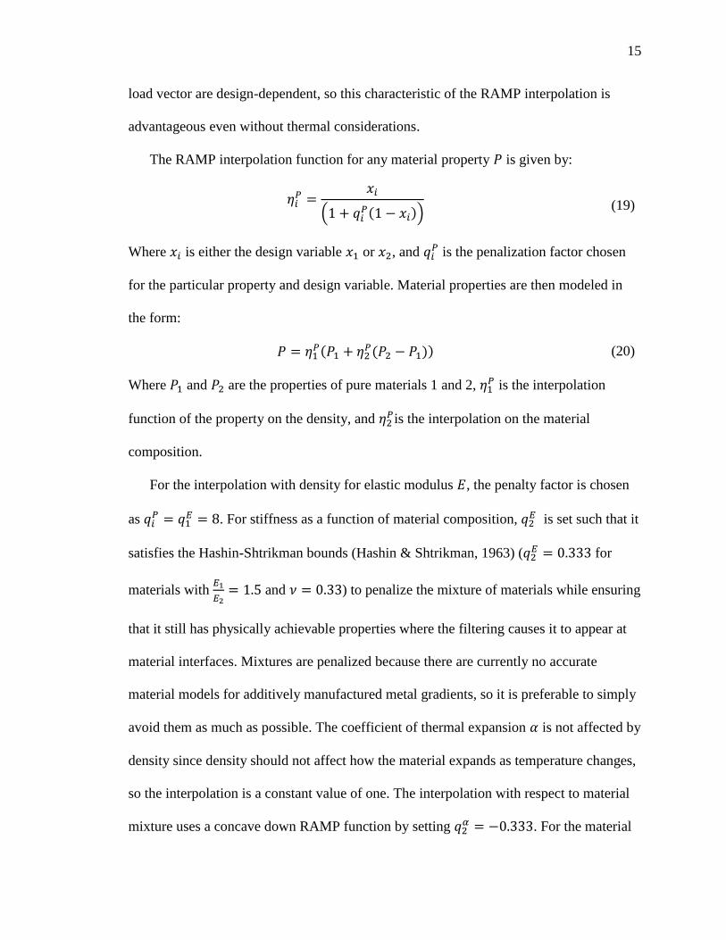
load vector are design-dependent, so this characteristic of the RAMP interpolation is
advantageous even without thermal considerations.
The RAMP interpolation function for any material property 𝑃 is given by:
𝜂𝑖𝑃 =
𝑥𝑖
(1 + 𝑞𝑖𝑃(1 − 𝑥𝑖))
(19)
Where 𝑥𝑖 is either the design variable 𝑥1 or 𝑥2, and 𝑞𝑖𝑃 is the penalization factor chosen
for the particular property and design variable. Material properties are then modeled in
the form:
𝑃 = 𝜂1𝑃(𝑃1 + 𝜂2
𝑃(𝑃2 − 𝑃1)) (20)
Where 𝑃1 and 𝑃2 are the properties of pure materials 1 and 2, 𝜂1𝑃 is the interpolation
function of the property on the density, and 𝜂2𝑃is the interpolation on the material
composition.
For the interpolation with density for elastic modulus 𝐸, the penalty factor is chosen
as 𝑞𝑖𝑃 = 𝑞1
𝐸 = 8. For stiffness as a function of material composition, 𝑞2𝐸 is set such that it
satisfies the Hashin-Shtrikman bounds (Hashin & Shtrikman, 1963) (𝑞2𝐸 = 0.333 for
materials with 𝐸1
𝐸2= 1.5 and 𝜈 = 0.33) to penalize the mixture of materials while ensuring
that it still has physically achievable properties where the filtering causes it to appear at
material interfaces. Mixtures are penalized because there are currently no accurate
material models for additively manufactured metal gradients, so it is preferable to simply
avoid them as much as possible. The coefficient of thermal expansion 𝛼 is not affected by
density since density should not affect how the material expands as temperature changes,
so the interpolation is a constant value of one. The interpolation with respect to material
mixture uses a concave down RAMP function by setting 𝑞2𝛼 = −0.333. For the material

16
strength, or maximum allowable stress 𝜎𝑎, the function with respect to density is also a
constant value of one. With respect to material composition, a concave up function with
𝑞2𝜎𝑎 = 0.333 is used. These interpolation functions used are summarized in Table 2.1.
Table 2.1
Material property interpolation functions.
Property Symbol Interpolation Functions
Elastic
Modulus 𝐸 𝜂1
𝐸 =𝑥1
(1 + 8(1 − 𝑥1)) 𝜂2
𝐸 =𝑥2
(1 + 0.333(1 − 𝑥2))
Coefficient
of Thermal
Expansion
𝛼 𝜂1𝛼 = 1 𝜂2
𝛼 =𝑥2
(1 − 0.333(1 − 𝑥2))
Allowable
Stress 𝜎𝑎 𝜂1
𝜎𝑎 = 1 𝜂2𝜎𝑎 =
𝑥2
(1 + 0.333(1 − 𝑥2))
2.4. Microstructure Thermoelastic Stress Analysis
The stress in the microstructure is computed at the center of each element using the
thermal stress equation:
𝝈𝑒 = 𝑪𝑒0𝜺𝑒 − 𝑪𝑒
0𝜶𝑒Δ𝑇 (21)
Where 𝑪𝑒0 is the solid element stiffness matrix of the element and Δ𝑇 is a uniform change
in temperature. The local strain field 𝜺 consists of an applied average macroscopic strain
�̅�, the fluctuating part of the mechanical strain 𝜺∗, and the thermal strain 𝜺𝛼. Since the
fluctuating strains 𝜺∗ are calculated from 𝝌 through Equation (5), which Equation (3)
shows is actually the negative of the fluctuating displacement field, it is subtracted from
�̅�. Substituting the full strain field with its constituents gives:
𝝈𝑒 = 𝑪𝑒0(�̅� − 𝜺𝑒
∗ + 𝜺𝑒𝛼) − 𝑪𝑒
0𝜶𝑒Δ𝑇 (22)

17
Rather than running a fifth independent finite element analysis with the prescribed
loads to find 𝜺𝑒∗ and 𝜺𝑒
𝛼, the results of the four finite element problems with unit strain
cases that were used to compute the homogenized properties 𝑪𝐻 and 𝜷𝐻 can be scaled to
the prescribed load magnitudes. The fluctuating mechanical strain subtracted from the
macroscopic strain can be rewritten in terms of the fluctuating mechanical strains caused
by the three unit macroscopic strains, and the thermal strain field caused by a unit
temperature change can be scaled to the strain field for the prescribed temperature
change:
𝝈𝑒 = 𝑪𝑒0((𝑰 − 𝜺𝑒
∗)�̅� + 𝜺𝑒𝛼Δ𝑇) − 𝑪𝑒
0𝜶𝑒Δ𝑇 (23)
Where 𝑰 is a 3x3 identity matrix representing the three unit macroscopic strain cases, 𝜺𝑒∗
now is a 3x3 matrix where each column is the fluctuating strain corresponding to the
cases in 𝑰, where the three fluctuating displacement fields were previously obtained from
the homogenization finite element analyses.
Writing the strains in (23) in terms of the previously obtained displacement fields
leads to the final equation for thermoelastic stress in the microstructure:
𝝈𝑒 = 𝑪𝑒0(𝑰 − 𝑩𝑒𝝌𝑒)�̅� + 𝑪𝑒
0(𝑩𝑒𝚪𝑒 − 𝜶𝑒)Δ𝑇 (24)
where 𝝌𝑒 contains three element displacement vectors and 𝚪𝑒 contains one.
The macroscopic strain �̅� is analogous to displacements applied to the boundaries if
its values are set to a constant. To apply a macroscopic stress �̅�, analogous to distributed
forces on the boundaries, the macroscopic strain corresponding to that stress is calculated
using the relationship:
�̅� = 𝑺𝐻�̅� + 𝜶𝐻𝛥𝑇 (25)
18
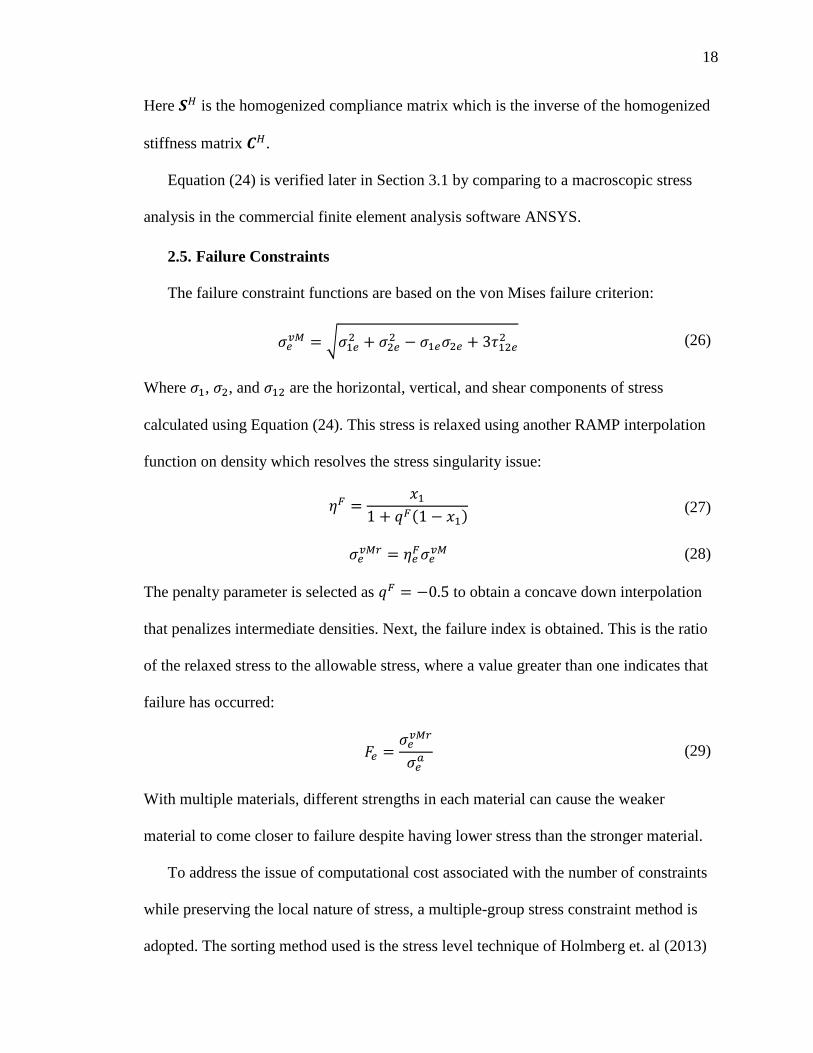
Here 𝑺𝐻 is the homogenized compliance matrix which is the inverse of the homogenized
stiffness matrix 𝑪𝐻.
Equation (24) is verified later in Section 3.1 by comparing to a macroscopic stress
analysis in the commercial finite element analysis software ANSYS.
2.5. Failure Constraints
The failure constraint functions are based on the von Mises failure criterion:
𝜎𝑒𝑣𝑀 = √𝜎1𝑒
2 + 𝜎2𝑒2 − 𝜎1𝑒𝜎2𝑒 + 3𝜏12𝑒
2 (26)
Where 𝜎1, 𝜎2, and 𝜎12 are the horizontal, vertical, and shear components of stress
calculated using Equation (24). This stress is relaxed using another RAMP interpolation
function on density which resolves the stress singularity issue:
𝜂𝐹 =𝑥1
1 + 𝑞𝐹(1 − 𝑥1) (27)
𝜎𝑒𝑣𝑀𝑟 = 𝜂𝑒
𝐹𝜎𝑒𝑣𝑀 (28)
The penalty parameter is selected as 𝑞𝐹 = −0.5 to obtain a concave down interpolation
that penalizes intermediate densities. Next, the failure index is obtained. This is the ratio
of the relaxed stress to the allowable stress, where a value greater than one indicates that
failure has occurred:
𝐹𝑒 =𝜎𝑒𝑣𝑀𝑟
𝜎𝑒𝑎 (29)
With multiple materials, different strengths in each material can cause the weaker
material to come closer to failure despite having lower stress than the stronger material.
To address the issue of computational cost associated with the number of constraints
while preserving the local nature of stress, a multiple-group stress constraint method is
adopted. The sorting method used is the stress level technique of Holmberg et. al (2013)

19
which places elements into equally sized groups based on failure index level, i.e. a certain
number 𝑛 of the elements closest to failure are placed in the first group, the next 𝑛
elements closest to failure are placed into the second group, and so on until all elements
are grouped. The last group may have a different number of elements.
After the elements are sorted, their failure indexes are aggregated into a single value
for each group using a p-norm function:
𝐹𝑚𝑃𝑁 = [
∑ (𝐹𝑒)𝑝𝑁𝑚
𝑒=1
𝑁𝑚]
1𝑝
(30)
Where 𝑚 is the group number, 𝑁𝑚 is the number of elements in the group, and 𝑝 is a
parameter that affects how close 𝐹𝑚𝑃𝑁 is to the maximum 𝐹𝑒 in the group. The larger 𝑝 is,
the closer they will be, but convergence issues will occur if it is too high. The value used
in this work is 𝑝 = 10. Since the p-norm function does not exactly capture the maximum
failure indexes in each group, using more groups can reduce the difference between the
averages and the maximum and lead to better control on the peak failure index. An
adaptive scale factor is then used to bring the p-norm values even closer to the highest
values (Deaton & Grandhi, 2016; Le et al., 2010) by using information from the previous
iteration (𝑘 − 1):
𝑠𝑚𝑘 =
max(𝐹𝑒)𝑘−1
(𝐹𝑚𝑃𝑁)𝑘−1 (31)
With each of the failure index groups aggregated by the p-norm function and adjusted
with the adaptive scale factors, the constraint functions are defined as follows:
𝑔𝑚(𝒙1, 𝒙2) = 𝑠𝑚𝑘 (𝐹𝑚
𝑃𝑁)𝑘 − 1 < 0 (32)
From numerical experiments, it was found that defining groups in only the first
iteration and maintaining this grouping for the remainder of the optimization gave the

20
best convergence characteristics. A quantity of three groups was used as it provided a
good balance between computational cost and instability caused by larger adaptive scale
factors.
2.6. Load Uncertainty
Since periodic microstructures are typically used to construct macrostructures that
experience many different internal stress states, constraining microstructure stress for a
single load case will not always make a cell robust enough for these applications. For
applications such as oriented microstructures (Allaire et al., 2019; Geoffroy-Donders et
al., 2020) or multi-scale optimization (Guo, Zhao, Zhang, Yan, & Sun, 2015), loads will
be known but there may be a certain amount of uncertainty in magnitude and direction.
For example, an orthotropic microstructure oriented to the principal stress directions
should never experience pure shear, however some variation of the nominal macroscopic
load will also cause variation in the internal stress states of the macrostructure. In these
cases with a limited number of stress states, Equation (24) can be evaluated multiple
times using different values for �̅� and Δ𝑇 to represent the possible variations. Failure
constraints can then be enforced on the stress distribution for each load case, improving
the microstructure’s stress tolerance for only the relevant cases.
Alternatively, if the possible loading conditions for the microstructure include many
different macroscopic stress states, worst-case mechanical stresses can be calculated
efficiently using an eigenvalue problem as first shown by Panetta et al. (2017) for the
shape optimization of single material microstructures. In this method the von Mises stress
at an element is expressed in matrix form as:
𝜎𝑒𝑣𝑀 = √�̅�𝑨𝑒𝑇𝑽𝑨𝑒�̅� (33)
21
Where:
𝑽 = [1 −1/2 0
−1/2 1 00 0 3
] (34)
and 𝑨𝑒 is the amplification matrix which maps the macroscopic stress �̅� to the
microscopic stress 𝝈𝑒 at the point:
𝑨𝑒 = 𝑪𝑒0(𝑰 − 𝜺𝑒
∗)𝑺𝐻 (35)
The maximum eigenvalue of the matrix 𝑨𝑒𝑇𝑽𝑨𝑒 is the worst-case von Mises stress at the
element, and the corresponding eigenvector represents the unit macroscopic stress vector
responsible for that stress. Performing this eigenvalue analysis for each element leads to a
different worst-case macroscopic stress vector and a different worst-case microscopic von
Mises stress at each element:
𝑠𝑒𝑣𝑀 = √�̅�𝑒𝑨𝑒𝑇𝑽𝑨𝑒�̅�𝑒 (36)
Similar to the von Mises stress calculated using Equation (24), the worst-case von
Mises stress distribution is relaxed, divided by the allowable stress to obtain worst-case
failure indexes, and aggregated with a p-norm function:
𝑠𝑒𝑣𝑀𝑟 = 𝜂𝑒
𝐹𝑠𝑒𝑣𝑀 (37)
𝐹𝑒𝑠 =
𝑠𝑒𝑣𝑀𝑟
𝜎𝑒𝑎 (38)
𝐹𝑠𝑃𝑁 = [
∑ (𝐹𝑒𝑠)𝑝𝑁
𝑒=1
𝑁]
1𝑝
(39)
The worst-case stress is minimized as an objective function, rather than used as
constraints, so only one group without a scale factor is used. In this work the p-norm
factor is set to 𝑝 = 3 when minimizing worst-case stress.

22
2.7. Manufacturing Uncertainty
Robustness with respect to uniform manufacturing uncertainties is implemented using
a multi-material extension of the methods presented by Sigmund (2009) and Silva et al.
(2019), which was also applied to single-material microstructures by Andreassen et al.
(2014). The value of the parameter 𝜂 in the threshold projection filter is adjusted to
higher and lower values 𝜂𝐸 = 0.75 and 𝜂𝐷 = 0.25 to generate uniformly “eroded” and
“dilated” versions of the density and composition variables:
�̅�𝑖𝑒𝐸 =
tanh(𝛽𝜂𝐸) + tanh(𝛽(�̃�𝑖𝑒 − 𝜂𝐸))
tanh(𝛽𝜂𝐸) + tanh(𝛽(1 − 𝜂𝐸))
�̅�𝑖𝑒𝐷 =
tanh(𝛽𝜂𝐷) + tanh(𝛽(�̃�𝑖𝑒 − 𝜂𝐷))
tanh(𝛽𝜂𝐷) + tanh(𝛽(1 − 𝜂𝐷))
(40)
Including the original physical variables created using 𝜂 = 0.5, there are now three
versions of each creating a total of nine different possible versions of the design. The
design constructed from the original variables �̅�1 and �̅�2 represents the “blueprint”, and
the eight others represent the possible variations that might occur with manufacturing
processes that uniformly over-build, under-build, over-mix, or under-mix the blueprint
design and its material composition.
With the eight additional designs representing uncertainty in manufacturing, new
objective and constraint functions of the eroded and dilated physical variables can be
defined that will lead to a more robust blueprint design. When taking the derivatives of
these functions, the chain rule is used with the corresponding projection filter:
23
𝜕𝑓 (�̅�𝑖𝐸(𝒙𝑖))
𝜕𝑥𝑖𝑗=∑
𝜕𝑓
𝜕�̅�𝑖𝑒𝐸
𝑒∈D
𝜕�̅�𝑖𝑒𝐸
𝜕�̃�𝑖𝑒
𝜕�̃�𝑖𝑒𝜕𝑥𝑖𝑗
𝜕𝑓 (�̅�𝑖𝐷(𝒙𝑖))
𝜕𝑥𝑖𝑗=∑
𝜕𝑓
𝜕�̅�𝑖𝑒𝐷
𝑒∈D
𝜕�̅�𝑖𝑒𝐷
𝜕�̃�𝑖𝑒
𝜕�̃�𝑖𝑒𝜕𝑥𝑖𝑗
(41)
2.8. Sensitivity Analysis
GCMMA requires the first derivatives with respect to the design variables 𝒙1 and 𝒙2
of the objective and constraint functions. These functions can include the homogenized
stiffness matrix, homogenized thermal expansion, homogenized thermal stress
coefficients, and material volume fractions, whose sensitivities have been shown
previously (Bendsoe & Sigmund, 2013; Sigmund & Torquato, 1997).
The failure constraint sensitivities are found by taking the derivative of the p-norm
stress function with respect to the density variables �̅�1 and the material composition
variables 𝒙2 (Deaton & Grandhi, 2016; Holmberg et al., 2013). The chain rule is utilized
while carrying through the summation sign, which is dropped for the terms that are
nonzero for only one element. The adjoint method is used for the terms containing
𝜕𝝌/𝜕�̅�𝑖𝑗 and 𝜕𝚪/𝜕�̅�𝑖𝑗, where the loads �̅� and Δ𝑇 can be factored out. The same adjoint
vector is found for each of these terms, so the adjoint vector is also factored out.
Applying these steps, the following sensitivities are obtained:
𝜕𝐹𝑚𝑃𝑁
𝜕�̅�1𝑗=𝜕𝐹𝑚
𝑃𝑁
𝜕𝐹𝑒
𝜕𝜂𝑒𝐹
𝜕�̅�1𝑗
𝜎𝑒𝑣𝑀
𝜎𝑒𝑎 + ∑
𝜕𝐹𝑚𝑃𝑁
𝜕𝐹𝑒
𝑁𝑚
𝑒=1
𝜂𝑒𝐹
𝜎𝑒𝑎
𝜕𝜎𝑒𝑣𝑀
𝜕𝝈𝑒𝑪𝑒0(𝑰 − 𝑩𝑒𝝌e)
𝜕�̅�
𝜕�̅�1𝑗
+ 𝝀𝜎𝑇 ((
𝜕𝑭𝑡ℎ
𝜕�̅�1𝑗−𝜕𝑲
𝜕�̅�1𝑗𝚪)Δ𝑇 − (
𝜕𝑭𝑚
𝜕�̅�1𝑗−𝜕𝑲
𝜕�̅�1𝑗𝝌) �̅�)
(42)

24
𝜕𝐹𝑚𝑃𝑁
𝜕�̅�2𝑗=𝜕𝐹𝑚
𝑃𝑁
𝜕𝐹𝑒
𝜂𝑒𝐹
𝜎𝑒𝑎
𝜕𝜎𝑒𝑣𝑀
𝜕𝝈𝑒
𝜕𝑪𝑒0
𝜕�̅�2𝑗((𝑰 − 𝑩𝑒𝝌𝑒)�̅� + (𝑩𝑒𝚪𝑒 − 𝜶𝑒)Δ𝑇)
−𝜕𝐹𝑚
𝑃𝑁
𝜕𝐹𝑒
𝜂𝑒𝐹
𝜎𝑒𝑎
𝜕𝜎𝑒𝑣𝑀
𝜕𝝈𝑒𝑪𝑒0𝜕𝜶𝑒𝜕�̅�2𝑗
Δ𝑇 −𝜕𝐹𝑚
𝑃𝑁
𝜕𝐹𝑒
𝜎𝑒𝑣𝑀𝑟
(𝜎𝑒𝑎)2
𝜕𝜎𝑒𝑎
𝜕�̅�2𝑗
+ ∑𝜕𝐹𝑚
𝑃𝑁
𝜕𝐹𝑒
𝑁𝑚
𝑒=1
𝜂𝑒𝐹
𝜎𝑒𝑎
𝜕𝜎𝑒𝑣𝑀
𝜕𝝈𝑒𝑪𝑒0(𝑰 − 𝑩𝑒𝝌e)
𝜕�̅�
𝜕�̅�2𝑗
+ 𝝀𝜎𝑇 ((
𝜕𝑭𝑡ℎ
𝜕�̅�2𝑗−𝜕𝑲
𝜕�̅�2𝑗𝚪)Δ𝑇 − (
𝜕𝑭𝑚
𝜕�̅�2𝑗−𝜕𝑲
𝜕�̅�2𝑗𝝌) �̅�)
(43)
Where:
𝜕𝐹𝑚𝑃𝑁
𝜕𝐹𝑒=(𝐹𝑚
𝑃𝑁)1−𝑝
𝑁𝑚(𝐹𝑒)
𝑝−1
𝜕�̅�
𝜕�̅�𝑖𝑗=𝜕𝑺𝐻
𝜕�̅�𝑖𝑗�̅� +
𝜕𝜶𝐻
𝜕�̅�𝑖𝑗Δ𝑇
𝜕𝑺𝐻
𝜕�̅�𝑖𝑗= −𝑺𝐻
𝜕𝑪𝐻
𝜕�̅�𝑖𝑗𝑺𝐻
(44)
The adjoint vector 𝝀𝜎 is calculated by assembling and solving the adjoint problem, once
for each group, using:
𝝀𝜎𝑲 = [∑𝜕𝐹𝑚
𝑃𝑁
𝜕𝐹𝑒
𝑁𝑚
𝑒=1
𝜂𝑒𝐹
𝜎𝑒𝑎
𝜕𝜎𝑒𝑣𝑀
𝜕𝝈𝑒𝑪𝑒0𝑩𝑒]
𝑇
(45)
The sensitivity of the worst-case stress p-norm function is similar up until the point
where the derivative of the worst-case stress is required:
𝜕𝐹𝑠𝑃𝑁
𝜕�̅�𝑖𝑗= 𝜕𝐹𝑠
𝑃𝑁
𝜕𝐹𝑒𝑠
𝑠𝑒𝑣𝑀
𝜎𝑒𝑎
𝜕𝜂𝑒𝐹
𝜕�̅�𝑖𝑗−𝜕𝐹𝑠
𝑃𝑁
𝜕𝐹𝑒𝑠
𝑠𝑒𝑣𝑀𝑟
(𝜎𝑒𝑎)2
𝜕𝜎𝑒𝑎
𝜕�̅�𝑖𝑗+∑
𝜕𝐹𝑠𝑃𝑁
𝜕𝐹𝑒𝑠
𝜂𝑒𝐹
𝜎𝑒𝑎
𝜕𝑠𝑒𝑣𝑀
𝜕�̅�𝑖𝑗
𝑁
𝑒=1
(46)

25
Since the macroscopic stress is not the same for every element, the chain rule is used to
write the equation in a form that allows for the use of the adjoint method on the term
containing 𝝌:
𝜕𝐹𝑠𝑃𝑁
𝜕�̅�𝑖𝑗= 𝜕𝐹𝑠
𝑃𝑁
𝜕𝐹𝑒𝑠
𝑠𝑒𝑣𝑀
𝜎𝑒𝑎
𝜕𝜂𝑒𝐹
𝜕�̅�𝑖𝑗−𝜕𝐹𝑠
𝑃𝑁
𝜕𝐹𝑒𝑠
𝑠𝑒𝑣𝑀𝑟
(𝜎𝑒𝑎)2
𝜕𝜎𝑒𝑎
𝜕�̅�𝑖𝑗
+∑𝜕𝐹𝑠
𝑃𝑁
𝜕𝐹𝑒𝑠
𝜂𝑒𝐹
𝜎𝑒𝑎 (𝜕𝑠𝑒
𝑣𝑀
𝜕𝑪𝑒0 ∶
𝜕𝑪𝑒0
𝜕�̅�𝑖𝑗+𝜕𝑠𝑒
𝑣𝑀
𝜕𝝌∶𝜕𝝌
𝜕�̅�𝑖𝑗+𝜕𝑠𝑒
𝑣𝑀
𝜕𝑺𝐻∶𝜕𝑺𝐻
𝜕�̅�𝑖𝑗)
𝑁
𝑒=1
(47)
Where:
𝜕𝑠𝑒𝑣𝑀
𝜕𝑪𝑒0 =
�̅�𝑒𝑇𝑨𝑒
𝑇𝑽
√�̅�𝑒𝑇𝑨𝑒𝑇𝑽𝑨𝑒�̅�𝑒⊗ (𝑰 − 𝑩𝑒𝝌𝑒)𝑺
𝐻�̅�𝑒
𝜕𝑠𝑒𝑣𝑀
𝜕𝝌𝑒= −
�̅�𝑒𝑇𝑨𝑒
𝑇𝑽𝑪𝑒0𝑩𝑒
√�̅�𝑒𝑨𝑒𝑇𝑽𝑨𝑒�̅�𝑒⊗𝑺𝐻�̅�𝑒
𝜕𝑠𝑒𝑣𝑀
𝜕𝑺𝐻=�̅�𝑒𝑇𝑨𝑒
𝑇𝑽𝑪𝑒0(𝑰 − 𝑩𝑒𝝌𝑒)
√�̅�𝑒𝑇𝑨𝑒𝑇𝑽𝑨𝑒�̅�𝑒⊗ �̅�𝑒
(48)
Here the macroscopic stress was treated as a constant since this is a derivative of an
eigenvalue with unit eigenvectors.
Substituting (48) into (47), using the adjoint method, and taking 𝑖 = 1 for the density
variables and 𝑖 = 2 for the composition variables leads to the final sensitivity equations
for the worst-case stress p-norm function:
𝜕𝐹𝑠𝑃𝑁
𝜕�̅�1𝑗= 𝜕𝐹𝑠
𝑃𝑁
𝜕𝐹𝑒𝑠
𝑠𝑒𝑣𝑀
𝜎𝑒𝑎
𝜕𝜂𝑒𝐹
𝜕�̅�1𝑗+∑
𝜕𝐹𝑠𝑃𝑁
𝜕𝐹𝑒𝑠
𝜂𝑒𝐹
𝜎𝑒𝑎
�̅�𝑒𝑇𝑨𝑒
𝑇𝑽𝑪𝑒0(𝑰 − 𝑩𝑒𝝌𝑒)
√�̅�𝑒𝑇𝑨𝑒
𝑇𝑽𝑨𝑒�̅�𝑒⊗ �̅�𝑒 ∶
𝜕𝑺𝐻
𝜕�̅�1𝑗
𝑁
𝑒=1
− 𝝀𝑠 ∶ (𝜕𝑭𝑚
𝜕�̅�1𝑗−𝜕𝑲
𝜕�̅�1𝑗𝝌𝑒)
(49)

26
𝜕𝐹𝑠𝑃𝑁
𝜕�̅�2𝑗= −
𝜕𝐹𝑠𝑃𝑁
𝜕𝐹𝑒𝑠
𝑠𝑒𝑣𝑀𝑟
(𝜎𝑒𝑎)2
𝜕𝜎𝑒𝑎
𝜕�̅�2𝑗+𝜕𝐹𝑠
𝑃𝑁
𝜕𝐹𝑒𝑠
𝜂𝑒𝐹
𝜎𝑒𝑎
�̅�𝑒𝑇𝑨𝑒
𝑇𝑽
√�̅�𝑒𝑇𝑨𝑒𝑇𝑽𝑨𝑒�̅�𝑒⊗ (𝑰 − 𝑩𝑒𝝌𝑒)𝑺
𝐻�̅�𝑒
∶𝜕𝑪𝑒
0
𝜕�̅�2𝑗+∑
𝜕𝐹𝑠𝑃𝑁
𝜕𝐹𝑒𝑠
𝜂𝑒𝐹
𝜎𝑒𝑎
�̅�𝑒𝑇𝑨𝑒
𝑇𝑽𝑪𝑒0(𝑰 − 𝑩𝑒𝝌𝑒)
√�̅�𝑒𝑇𝑨𝑒𝑇𝑽𝑨𝑒�̅�𝑒⊗ �̅�𝑒 ∶
𝜕𝑺𝐻
𝜕�̅�2𝑗
𝑁
𝑒=1
− 𝝀𝑠 ∶ (𝜕𝑭𝑚
𝜕�̅�2𝑗−𝜕𝑲
𝜕�̅�2𝑗𝝌𝑒)
(50)
𝝀𝑠𝑲 = [∑𝜕𝐹𝑠
𝑃𝑁
𝜕𝐹𝑒𝑠
𝜂𝑒𝐹
𝜎𝑒𝑎
�̅�𝑒𝑇𝑨𝑒
𝑇𝑽𝑪𝑒0𝑩𝑒
√�̅�𝑒𝑨𝑒𝑇𝑽𝑨𝑒�̅�𝑒
⊗𝑺𝐻�̅�𝑒
𝑁
𝑒=1
]
𝑇
(51)
27
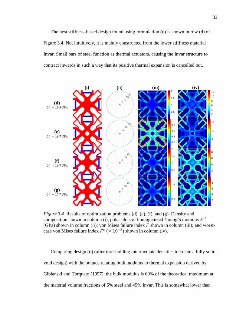
3. Metamaterial Topology Optimization: Numerical Examples
In this section, the framework is used to design several microstructure test cases made
from additively manufactured stainless steel 304L and Invar 36 (Hofmann, Roberts, et al.,
2014; Z. Wang, Palmer, & Beese, 2016). The properties used for the examples are shown
in Table 3.1.
Table 3.1
Material properties of stainless steel 304L and Invar 36.
Properties Stainless Steel 304L Invar 36
Elastic Modulus, 𝐸 (𝐺𝑃𝑎) 240 160
Poisson’s Ratio, 𝜈 0.33 0.33
Coefficient of Thermal Expansion, 𝛼 (10−6/°𝐶) 15 1.5
Allowable Stress, 𝜎𝑎 (𝑀𝑃𝑎) 400 250
(Hofmann, Roberts, et al., 2014; Z. Wang et al., 2016)
The multi-material microstructure topology optimization problem is highly non-
convex, with many different possible material layouts that can achieve the desired
macroscopic properties. This makes the algorithm very susceptible to finding local
minimums. Several strategies for dealing with this local minimum problem were
suggested by Sigmund and Torquato (1997), and similar ones are also used here to help
find better local minimums which are hopefully global optimums (although this cannot be
guaranteed). Lines of geometric symmetry are enforced to reduce the space of possible
designs and aid in achieving the desired symmetry in material properties, and the density
filter is used to smooth out local minimums at the beginning of the optimizations by
applying it twice to the starting design in the first iteration.

28
Another issue is that even if a reasonable local minimum is found there may still be
others that give similar performance, making it difficult to evaluate how the stress-based
formulations influence the designs. To avoid this problem, the optimizations are first
performed without any stress-based functions to find fully optimized stiffness-based
designs. The stiffness-based optimizations are ran repeatedly with different initial
conditions, and the best results are then chosen as the starting points for all subsequent
stress-based optimizations. Starting with an optimized stiffness-based design ensures that
any further changes are due to the effects of stress or uncertainty considerations, and not
because the algorithm has simply found a different local minimum.
Each of the following examples are two dimensional square cells of unit length,
width, and thickness. The cells are meshed with a grid of 100x100 plane stress elements.
The optimizations were considered converged when the change in each design variable
was less than 0.001. Invar 36 and stainless steel 304L are represented in the design plots
by red and blue colors, respectively, with mixtures shown by the gradient between the
two colors which is demonstrated in Figure 3.1. Density is represented by the opacity of
the elements, making void space appear white.
Figure 3.1 Color representation of the composition variable 𝒙2 for plots of designs made
from Invar 36, stainless steel 304L, and their mixtures.

29
3.1. Thermoelastic Stress Analysis Verification
To verify that Equation (24) is accurate, a macroscopic finite element model
consisting of a grid of several multi-material square cells with square holes was analyzed
in ANSYS as a standard mechanics approach. Displacements were applied to the
boundaries equivalent to a macroscopic strain of �̅� = [0 −0.01 0]𝑇. The strain
components 휀1̅ = 0 and 휀1̅2 = 0 were replicated by fixing the horizontal displacements of
the left and right boundaries, and 휀2̅ = −0.01 was applied by fixing the vertical
displacement of the bottom boundary and by applying a compressive displacement of one
hundredth of the macrostructure’s total height to the top boundary. A uniform thermal
condition of Δ𝑇 = 100℃ was also applied to the entire macrostructure. The same
conditions were evaluated using the homogenization-based thermal stress Equation (24).
The practically identical results are shown in Figure 3.2.
(a) (b) (c)
Figure 3.2 Thermal and mechanical stress computed using the presented
homogenization-based formulation compared to a standard mechanics analysis in
ANSYS. (a) The cell geometry and composition; (b) the microscopic stress computed
using the homogenization-based formula; and (c) the stress computed using ANSYS
showing a single cell at the center of the macrostructure.

30
3.2. Maximum Orthotropic Stiffness Single-Material Microstructure
The first optimization example is a typical orthotropic lattice structure commonly
used in other studies on periodic microstructures (Coelho et al., 2019; Collet et al., 2018;
Sigmund, 2000). The stiffness-based design is found using the following optimization
formulation:
(a) Maximization of stiffness 𝐶11𝐻 + 𝐶22
𝐻 subjected to a volume fraction of 60%.
𝑚𝑎𝑥𝑖𝑚𝑖𝑧𝑒: 𝐶11𝐻 + 𝐶22
𝐻
𝑠𝑢𝑏𝑗𝑒𝑐𝑡𝑒𝑑 𝑡𝑜: 𝑉𝑓 = 0.6 (52)
Without any requirements imposed on thermal expansion, the optimization converges to
pure steel and achieves a homogenized stiffness of 𝐶11𝐻 = 95.6 𝐺𝑃𝑎. The design is
analyzed by computing the homogenized Young’s modulus in all directions, performing a
stress analysis using a macroscopic stress state of �̅� = [−114 −114 0]𝑇 𝑀𝑃𝑎, and
performing a worst-case stress analysis. The optimized design, homogenized Young’s
modulus polar plots, and stress analysis results are shown in Figure 3.3, row (a). The
maximum microscopic stress is 7% higher than the steel’s allowable stress, which occurs
at the sharpest points of the hole’s corners. For the worst-case microscopic stress
distribution most stress eigenvectors are close to a pure shear state, with the maximum
corresponding to the eigenvector �̅�𝑒 = [0.11 0.11 0.99]𝑇 𝑃𝑎.
Next, failure constraints are included in the formulation:
(b) Maximization of stiffness 𝐶11𝐻 + 𝐶22
𝐻 subjected to a volume fraction of 60% and the
failure constraints using the applied load of �̅� = [−114 −114 0]𝑇 𝑀𝑃𝑎.
Row (b) of Figure 3.3 shows that the stress constraints bring the microscopic stress down
to the same value as the allowable stress by slightly increasing the radius of the corners at

31
a small cost to stiffness, a result similar to that achieved by Collet et al. (2018). The
maximum worst-case stress is also reduced as a side effect.
(i) (ii) (iii) (iv)
(a) 𝐶11𝐻 = 95.6 𝐺𝑃𝑎
(b) 𝐶11𝐻 = 95.1 𝐺𝑃𝑎
(c) 𝐶11𝐻 = 95.1 𝐺𝑃𝑎
Figure 3.3 Results of optimization problems (a), (b), and (c). Density and composition
shown in column (i); polar plots of homogenized Young’s modulus 𝐸𝐻 (GPa) shown in
column (ii); von Mises failure index 𝐹 shown in column (iii); and worst-case von Mises
failure index 𝐹𝑠 (× 10−8) shown in column (iv).
The third formulation for the single-material orthotropic microstructure is a
minimization of the worst-case stresses:
(c) Minimization of 𝐹𝑠𝑃𝑁 subjected to a volume fraction of 60% and lower bounds on
the stiffness 𝐶11𝐻 and 𝐶22
𝐻 equal to that of design (b), 𝐶11𝐻 = 95.1 𝐺𝑃𝑎.
Minimizing the worst-case stress increases the shear strength of the cell by creating a
more circular shape and a stiffness polar plot that is slightly closer to isotropic. The
maximum worst-case stress is reduced by 23% compared to design (a), however this is at
the cost of increasing the maximum stress from the hydrostatic load to 8% higher than the

32
allowable. This is due to not including a failure constraint for the specific load case.
Consequently, this shows that worst-case stress minimization may not strengthen the cell
for all load cases simultaneously. If it is known that the microstructure will never
experience the worst-case states, it will be better to optimize for a single load case, or a
few load cases, using Equation (24) and failure constraint functions (32). Otherwise,
worst-case stress minimization can make a more robust structure since the maximum
worst-case stresses are larger than the maximum stresses of other load cases.
3.3. Maximum Isotropic Stiffness, Zero Thermal Expansion Microstructure
The second example is a thermoelastic metamaterial that will not expand or shrink
when its temperature changes. Special properties such as this are achievable by taking
advantage of the mismatch in thermal expansion properties between steel and Invar. This
mismatch also introduces thermal stresses which are induced by Δ𝑇.
The stiffness-based design is generated using the following formulation:
(d) Maximization of stiffness 𝐶11𝐻 + 𝐶22
𝐻 subjected to a volume fraction of 50%,
homogenized coefficients of thermal expansion of zero, and isotropic homogenized
stiffness. Horizontal, vertical, and diagonal geometric symmetry is enforced.
𝑚𝑎𝑥𝑖𝑚𝑖𝑧𝑒: 𝐶11𝐻 + 𝐶22
𝐻
𝑠𝑢𝑏𝑗𝑒𝑐𝑡𝑒𝑑 𝑡𝑜:
{
𝐺𝑒𝑜𝑚𝑒𝑡𝑟𝑖𝑐 𝑆𝑦𝑚𝑚𝑒𝑡𝑟𝑦:𝐻𝑜𝑟𝑖𝑧𝑜𝑛𝑡𝑎𝑙, 𝑣𝑒𝑟𝑡𝑖𝑐𝑎𝑙, 𝑎𝑛𝑑 𝑑𝑖𝑎𝑔𝑜𝑛𝑎𝑙
𝑉𝑓 = 0.5
𝛼11𝐻 < 0
𝛼22𝐻 < 0
(𝐶11𝐻 + 𝐶22
𝐻 − 2(𝐶12𝐻 + 2𝐶33
𝐻 ))2
(𝐶11𝐻 + 𝐶22
𝐻 )2+(𝐶11
𝐻 − 𝐶22𝐻 )2
(𝐶11𝐻 + 𝐶22
𝐻 )2< 0.001
(53)
33
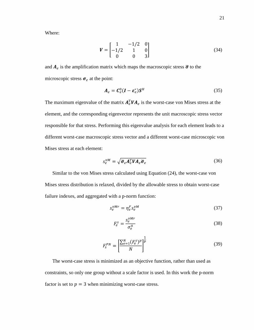
The best stiffness-based design found using formulation (d) is shown in row (d) of
Figure 3.4. Not intuitively, it is mainly constructed from the lower stiffness material
Invar. Small bars of steel function as thermal actuators, causing the Invar structure to
contract inwards in such a way that its positive thermal expansion is cancelled out.
(i) (ii) (iii) (iv)
(d) 𝐶11𝐻 = 19.8 𝐺𝑃𝑎
(e) 𝐶11𝐻 = 16.7 𝐺𝑃𝑎
(f) 𝐶11𝐻 = 16.7 𝐺𝑃𝑎
(g) 𝐶11𝐻 = 17.7 𝐺𝑃𝑎
Figure 3.4 Results of optimization problems (d), (e), (f), and (g). Density and
composition shown in column (i); polar plots of homogenized Young’s modulus 𝐸𝐻
(GPa) shown in column (ii); von Mises failure index 𝐹 shown in column (iii); and worst-
case von Mises failure index 𝐹𝑠 (× 10−8) shown in column (iv).
Comparing design (d) (after thresholding intermediate densities to create a fully solid-
void design) with the bounds relating bulk modulus to thermal expansion derived by
Gibianski and Torquato (1997), the bulk modulus is 60% of the theoretical maximum at
the material volume fractions of 5% steel and 45% Invar. This is somewhat lower than

34
85% of the bound achieved by Sigmund and Torquato (1997) for a 25%-25% volume
fraction microstructure, however the absolute bulk modulus of design (d) is
approximately 35% higher after accounting for the difference in the constituent material
stiffness ratio by using a weighted average. Computing the bounds for every possible
volume fraction combination in Figure 3.5 shows that low volume fractions of steel and
high volume fractions of Invar are indeed necessary to achieve optimal bulk modulus.
Designs with bulk modulus closer to the bounds are likely possible by using a smaller
filter radius and relaxing the geometric symmetry constraints.
Figure 3.5 The upper bounds of bulk modulus (Pa) for zero thermal expansion isotropic
microstructures of every possible volume fraction. The highest values occur for large
volume fractions of Invar, the weaker of the two materials.

35
Stress analysis is performed on design (d) with a macroscopic stress of �̅� =
[−20 −20 0]𝑇 𝑀𝑃𝑎 and a temperature change of Δ𝑇 = 100 °𝐶, showing stress
concentrations double the allowable stress in the thin Invar members in Figure 3.4. The
worst-case stresses also show similar concentrations, with high failure index also present
throughout more of the structure compared to the specific load case. The failure
constraints are then added to the optimization formulation:
(e) The same as problem (d) with failure constraints on the applied loads of �̅� =
[−20 −20 0]𝑇 𝑀𝑃𝑎 and Δ𝑇 = 100 °𝐶.
The results of optimization formulation (e) are shown in row (e) of Figure 3.4. Activating
the stress constraints here brings the maximum stress down to the allowable stress at a
cost of decreasing the stiffness by 16%. A hole appears in the center where previously
there was low stress, and this material is distributed elsewhere to reinforce more highly
stressed areas while satisfying the constraint on volume (𝑉𝑓 = 0.5). Small spots of high
strength steel appear where the stress concentrations existed in design (d). The design is
also more evenly stressed for the chosen load case, however the maximum worst-case
stress (corresponding to �̅�𝑒 = [−0.19 −0.01 −0.98]𝑇 𝑃𝑎) increases. Since this is an
isotropic microstructure, it would be advantageous to make use of its robust stiffness by
subjecting it to loads in any direction. Therefore, a worst-case stress minimization for
robust strength is probably the best choice of stress-based methods:
(f) Minimization of 𝐹𝑠𝑃𝑁 subjected to a volume fraction of 50%, homogenized
coefficients of thermal expansion of zero, isotropic homogenized stiffness, and a
lower bound on stiffness equal to the result of problem (e). Horizontal, vertical, and
diagonal geometric symmetry is enforced.

36
The worst-case stress minimization of problem (f), shown in row (f) of Figure 3.4,
results in a cell without a central hole, several more areas with reinforcing steel, thicker
thin members at the corners, and an overall smoother geometry. The maximum worst-
case stress is reduced by 12% and its overall distribution is much more even. The thermal
expansion is zero, however the newly introduced reinforcing steel is only present as thin
edges and small spots. These would be extremely difficult to manufacture accurately for
small cell sizes, and given that the steel controls the macroscopic thermal expansion, any
inaccuracy would likely ruin the zero thermal expansion property. To investigate this, the
manufacturing uncertainty method of Section 2.7 is applied to design (f) and shown in
Figure 3.6 with the uncertain designs’ thermal expansions and worst-case stress
distributions. The thermal expansion reduces to as much as −0.6𝛼𝐼𝑛𝑣𝑎𝑟 for the design
uncertainty of eroded density and dilated composition, and increases up to 2.1𝛼𝐼𝑛𝑣𝑎𝑟 for
the dilated density and eroded composition uncertainty. The eroded density uncertainties
also have significantly increased worst-case stress due to the thinner geometry.
To control the thermal expansion and stress when manufacturing uncertainty is
present, the following formulation is used:
(g) Minimization of the sum of blueprint and manufacturing uncertainty design worst-
case stress functions 𝐹𝑠𝑃𝑁 subjected to the same constraints as problem (f), and also
subjected to thermal expansion constraints −0.35 <𝛼𝐻
𝛼𝐼𝑛𝑣𝑎𝑟< 0.35 on each of the
eight manufacturing uncertainty designs.
The resulting design, shown in row (g) of Figure 3.4, is less complex than design (f),
with fewer spots of reinforcing steel introduced due to the robust thermal expansion
constraints. Instead of by adding steel to the mixture, the stress is reduced by rounding
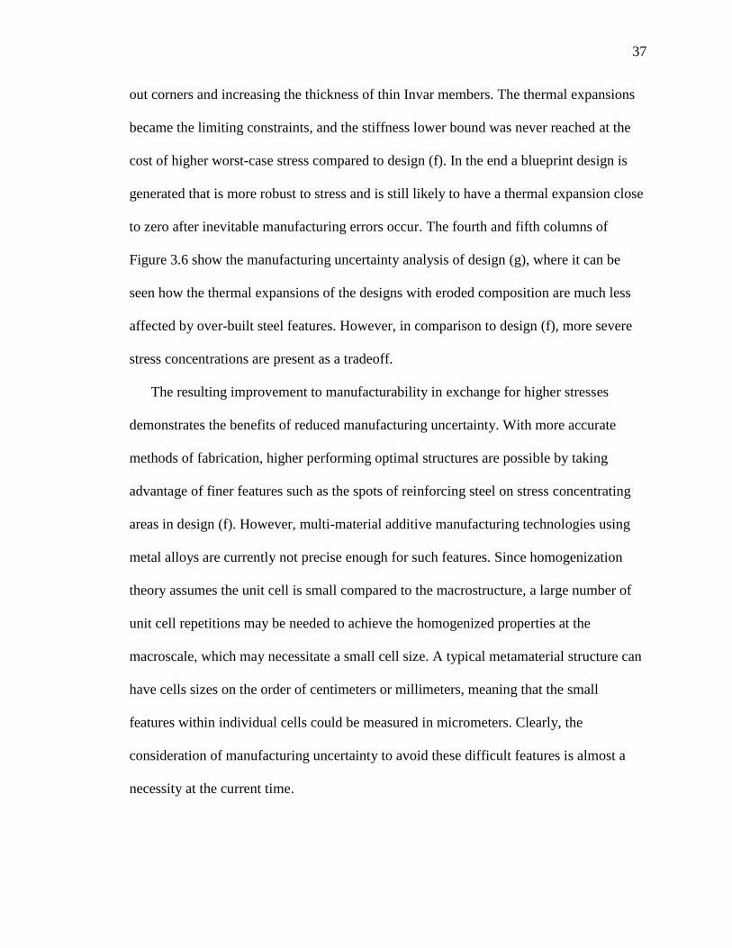
37
out corners and increasing the thickness of thin Invar members. The thermal expansions
became the limiting constraints, and the stiffness lower bound was never reached at the
cost of higher worst-case stress compared to design (f). In the end a blueprint design is
generated that is more robust to stress and is still likely to have a thermal expansion close
to zero after inevitable manufacturing errors occur. The fourth and fifth columns of
Figure 3.6 show the manufacturing uncertainty analysis of design (g), where it can be
seen how the thermal expansions of the designs with eroded composition are much less
affected by over-built steel features. However, in comparison to design (f), more severe
stress concentrations are present as a tradeoff.
The resulting improvement to manufacturability in exchange for higher stresses
demonstrates the benefits of reduced manufacturing uncertainty. With more accurate
methods of fabrication, higher performing optimal structures are possible by taking
advantage of finer features such as the spots of reinforcing steel on stress concentrating
areas in design (f). However, multi-material additive manufacturing technologies using
metal alloys are currently not precise enough for such features. Since homogenization
theory assumes the unit cell is small compared to the macrostructure, a large number of
unit cell repetitions may be needed to achieve the homogenized properties at the
macroscale, which may necessitate a small cell size. A typical metamaterial structure can
have cells sizes on the order of centimeters or millimeters, meaning that the small
features within individual cells could be measured in micrometers. Clearly, the
consideration of manufacturing uncertainty to avoid these difficult features is almost a
necessity at the current time.
38
Uncertainty Design (f) 𝑭𝑠 (× 10−8) Design (g) 𝑭𝑠 (× 10−8)
�̅�1𝐸 , �̅�2
𝐸
𝛼𝐻 𝛼𝐼𝑛𝑣𝑎𝑟⁄ = +0.089 𝛼𝐻 𝛼𝐼𝑛𝑣𝑎𝑟⁄ = −0.32
𝒙1𝐸 , 𝒙2
𝛼𝐻 𝛼𝐼𝑛𝑣𝑎𝑟⁄ = −0.54 𝛼𝐻 𝛼𝐼𝑛𝑣𝑎𝑟⁄ = −0.29
𝒙1𝐸 , 𝒙2
𝐷
𝛼𝐻 𝛼𝐼𝑛𝑣𝑎𝑟⁄ = −0.60 𝛼𝐻 𝛼𝐼𝑛𝑣𝑎𝑟⁄ = −0.18
�̅�1, �̅�2𝐸
𝛼𝐻 𝛼𝐼𝑛𝑣𝑎𝑟⁄ = +0.98 𝛼𝐻 𝛼𝐼𝑛𝑣𝑎𝑟⁄ = −0.00
�̅�1, �̅�2𝐷
𝛼𝐻 𝛼𝐼𝑛𝑣𝑎𝑟⁄ = −0.23 𝛼𝐻 𝛼𝐼𝑛𝑣𝑎𝑟⁄ = +0.08
𝒙1𝐷 , �̅�2
𝐸
𝛼𝐻 𝛼𝐼𝑛𝑣𝑎𝑟⁄ = +2.10 𝛼𝐻 𝛼𝐼𝑛𝑣𝑎𝑟⁄ = +0.35
�̅�1𝐷 , �̅�2
𝛼𝐻 𝛼𝐼𝑛𝑣𝑎𝑟⁄ = +0.76 𝛼𝐻 𝛼𝐼𝑛𝑣𝑎𝑟⁄ = +0.30
�̅�1𝐷 , �̅�2
𝐷
𝛼𝐻 𝛼𝐼𝑛𝑣𝑎𝑟⁄ = +0.27 𝛼𝐻 𝛼𝐼𝑛𝑣𝑎𝑟⁄ = +0.35
Figure 3.6 Uniform manufacturing uncertainties of designs (f) and (g) with their
homogenized thermal expansions and worst-case stress distributions.

39
3.4. Negative Thermal Expansion Microstructure
The third example is a low-stiffness thermoelastic metamaterial with a thermal
expansion that is as negative as possible:
(h) Minimization of thermal expansion 𝛼1𝐻 + 𝛼2
𝐻 subjected to a volume fraction of 50%
and small lower bounds on stiffness. Horizontal, vertical, and diagonal geometric
symmetry is enforced.
𝑚𝑖𝑛𝑖𝑚𝑖𝑧𝑒: 𝛼11𝐻 + 𝛼22
𝐻
𝑠𝑢𝑏𝑗𝑒𝑐𝑡𝑒𝑑 𝑡𝑜:
{
𝐺𝑒𝑜𝑚𝑒𝑡𝑟𝑖𝑐 𝑆𝑦𝑚𝑚𝑒𝑡𝑟𝑦:𝐻𝑜𝑟𝑖𝑧𝑜𝑛𝑡𝑎𝑙, 𝑣𝑒𝑟𝑡𝑖𝑐𝑎𝑙, 𝑎𝑛𝑑 𝑑𝑖𝑎𝑔𝑜𝑛𝑎𝑙
𝑉𝑓 = 0.5
𝐶11𝐻 + 𝐶22
𝐻 > 0.02(𝐶11𝑆𝑡𝑒𝑒𝑙 + 𝐶22
𝑆𝑡𝑒𝑒𝑙)
𝐶12𝐻 > 0.02𝐶12
𝑆𝑡𝑒𝑒𝑙
𝐶33𝐻 > 0.002𝐶33
𝑆𝑡𝑒𝑒𝑙
(54)
The stiffness-based design created by optimization problem (h) and its analysis is
shown in row (h) of Figure 3.7. The design consists of four composite beam-like
structures connected by thin compliant hinges. As the steel sides of the beams expand
more than the Invar sides, the beams bend inwards to create the macroscopically negative
thermal expansion of the metamaterial. The stress analysis is performed with a
macroscopic stress of �̅� = [18 18 0]𝑇 𝑀𝑃𝑎 and a temperature change of Δ𝑇 =
100 °𝐶. The chosen tensile load pulling against the contraction caused by the temperature
increase produces stress concentrations at the hinges 2.7 times the allowable stress. The
structure is highly orthotropic, and as such the worst-case stresses dominate at the thin
hinge points of the compliant mechanism-like cell and are maximum for an almost pure
shear stress state of �̅�𝑒 = [−0.03 −0.09 0.99]𝑇 𝑃𝑎.
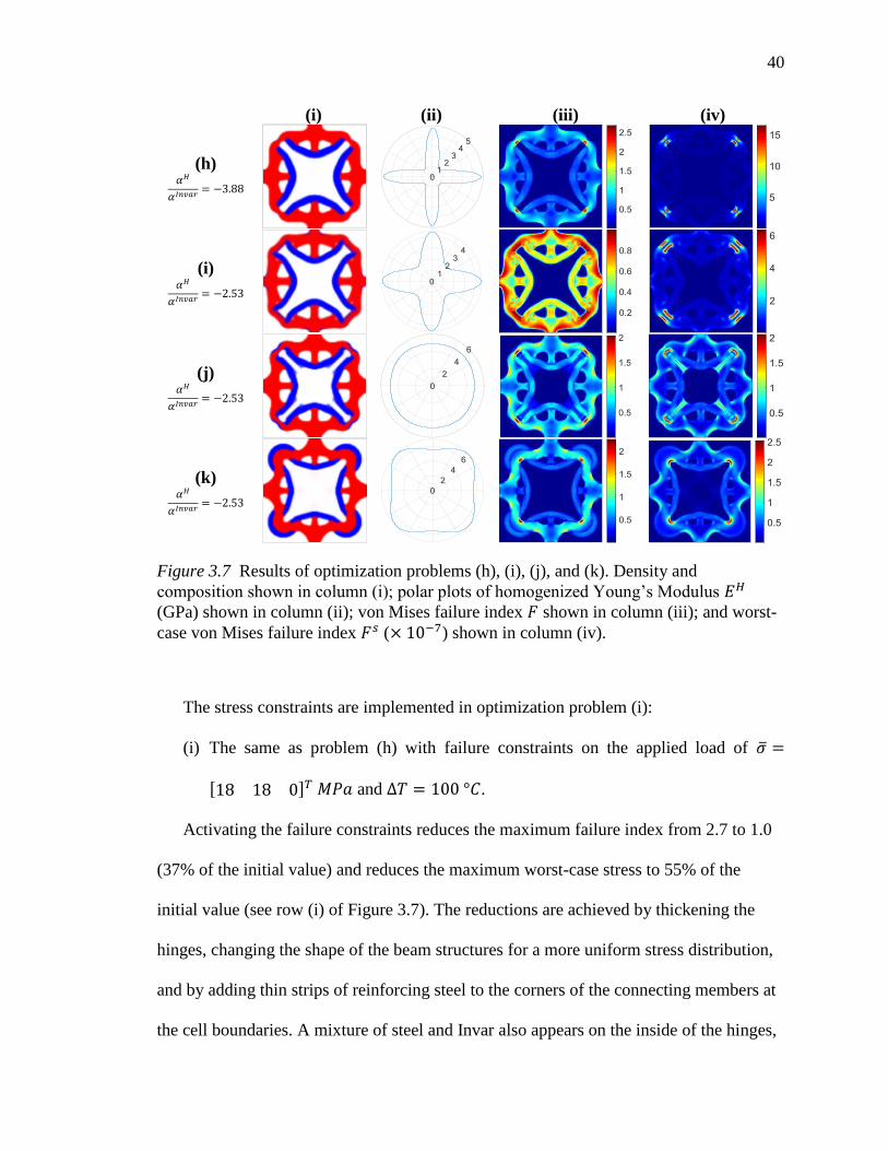
40
(i) (ii) (iii) (iv)
(h) 𝛼𝐻
𝛼𝐼𝑛𝑣𝑎𝑟= −3.88
(i) 𝛼𝐻
𝛼𝐼𝑛𝑣𝑎𝑟= −2.53
(j) 𝛼𝐻
𝛼𝐼𝑛𝑣𝑎𝑟= −2.53
(k) 𝛼𝐻
𝛼𝐼𝑛𝑣𝑎𝑟= −2.53
Figure 3.7 Results of optimization problems (h), (i), (j), and (k). Density and
composition shown in column (i); polar plots of homogenized Young’s Modulus 𝐸𝐻
(GPa) shown in column (ii); von Mises failure index 𝐹 shown in column (iii); and worst-
case von Mises failure index 𝐹𝑠 (× 10−7) shown in column (iv).
The stress constraints are implemented in optimization problem (i):
(i) The same as problem (h) with failure constraints on the applied load of 𝜎 =
[18 18 0]𝑇 𝑀𝑃𝑎 and Δ𝑇 = 100 °𝐶.
Activating the failure constraints reduces the maximum failure index from 2.7 to 1.0
(37% of the initial value) and reduces the maximum worst-case stress to 55% of the
initial value (see row (i) of Figure 3.7). The reductions are achieved by thickening the
hinges, changing the shape of the beam structures for a more uniform stress distribution,
and by adding thin strips of reinforcing steel to the corners of the connecting members at
the cell boundaries. A mixture of steel and Invar also appears on the inside of the hinges,
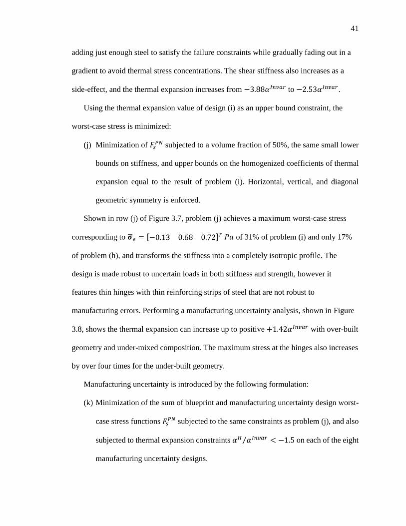
41
adding just enough steel to satisfy the failure constraints while gradually fading out in a
gradient to avoid thermal stress concentrations. The shear stiffness also increases as a
side-effect, and the thermal expansion increases from −3.88𝛼𝐼𝑛𝑣𝑎𝑟 to −2.53𝛼𝐼𝑛𝑣𝑎𝑟.
Using the thermal expansion value of design (i) as an upper bound constraint, the
worst-case stress is minimized:
(j) Minimization of 𝐹𝑠𝑃𝑁 subjected to a volume fraction of 50%, the same small lower
bounds on stiffness, and upper bounds on the homogenized coefficients of thermal
expansion equal to the result of problem (i). Horizontal, vertical, and diagonal
geometric symmetry is enforced.
Shown in row (j) of Figure 3.7, problem (j) achieves a maximum worst-case stress
corresponding to �̅�𝑒 = [−0.13 0.68 0.72]𝑇 𝑃𝑎 of 31% of problem (i) and only 17%
of problem (h), and transforms the stiffness into a completely isotropic profile. The
design is made robust to uncertain loads in both stiffness and strength, however it
features thin hinges with thin reinforcing strips of steel that are not robust to
manufacturing errors. Performing a manufacturing uncertainty analysis, shown in Figure
3.8, shows the thermal expansion can increase up to positive +1.42𝛼𝐼𝑛𝑣𝑎𝑟 with over-built
geometry and under-mixed composition. The maximum stress at the hinges also increases
by over four times for the under-built geometry.
Manufacturing uncertainty is introduced by the following formulation:
(k) Minimization of the sum of blueprint and manufacturing uncertainty design worst-
case stress functions 𝐹𝑠𝑃𝑁 subjected to the same constraints as problem (j), and also
subjected to thermal expansion constraints 𝛼𝐻 𝛼𝐼𝑛𝑣𝑎𝑟⁄ < −1.5 on each of the eight
manufacturing uncertainty designs.
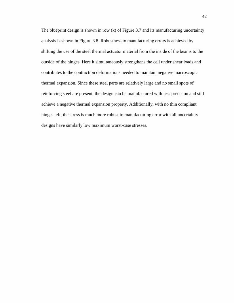
42
The blueprint design is shown in row (k) of Figure 3.7 and its manufacturing uncertainty
analysis is shown in Figure 3.8. Robustness to manufacturing errors is achieved by
shifting the use of the steel thermal actuator material from the inside of the beams to the
outside of the hinges. Here it simultaneously strengthens the cell under shear loads and
contributes to the contraction deformations needed to maintain negative macroscopic
thermal expansion. Since these steel parts are relatively large and no small spots of
reinforcing steel are present, the design can be manufactured with less precision and still
achieve a negative thermal expansion property. Additionally, with no thin compliant
hinges left, the stress is much more robust to manufacturing error with all uncertainty
designs have similarly low maximum worst-case stresses.

43
Uncertainty Design (j) 𝑭𝑠 (× 10−7) Design (k) 𝑭𝑠 (× 10−7)
�̅�1𝐸 , �̅�2
𝐸
𝛼𝐻 𝛼𝐼𝑛𝑣𝑎𝑟⁄ = −4.69 𝛼𝐻 𝛼𝐼𝑛𝑣𝑎𝑟⁄ = −3.06
�̅�1𝐸 , �̅�2
𝛼𝐻 𝛼𝐼𝑛𝑣𝑎𝑟⁄ = −5.16 𝛼𝐻 𝛼𝐼𝑛𝑣𝑎𝑟⁄ = −3.13
�̅�1𝐸 , �̅�2
𝐷
𝛼𝐻 𝛼𝐼𝑛𝑣𝑎𝑟⁄ = −4.96 𝛼𝐻 𝛼𝐼𝑛𝑣𝑎𝑟⁄ = −2.82
𝒙1, �̅�2𝐸
𝛼𝐻 𝛼𝐼𝑛𝑣𝑎𝑟⁄ = −2.02 𝛼𝐻 𝛼𝐼𝑛𝑣𝑎𝑟⁄ = −2.32
𝒙1, 𝒙2𝐷
𝛼𝐻 𝛼𝐼𝑛𝑣𝑎𝑟⁄ = −2.67 𝛼𝐻 𝛼𝐼𝑛𝑣𝑎𝑟⁄ = −2.39
�̅�1𝐷 , 𝒙2
𝐸
𝛼𝐻 𝛼𝐼𝑛𝑣𝑎𝑟⁄ = +1.42 𝛼𝐻 𝛼𝐼𝑛𝑣𝑎𝑟⁄ = −1.50
�̅�1𝐷 , �̅�2
𝛼𝐻 𝛼𝐼𝑛𝑣𝑎𝑟⁄ = +1.03 𝛼𝐻 𝛼𝐼𝑛𝑣𝑎𝑟⁄ = −1.79
𝒙1𝐷 , �̅�2
𝐷
𝛼𝐻 𝛼𝐼𝑛𝑣𝑎𝑟⁄ = +0.68 𝛼𝐻 𝛼𝐼𝑛𝑣𝑎𝑟⁄ = −1.78
Figure 3.8 Uniform manufacturing uncertainties of designs (j) and (k) with their
homogenized thermal expansions and worst-case stress distributions.

44
4. Lattice Structures: Numerical Analysis
In this section, basic mechanical orthotropic lattice structures are analyzed in the
context of using them to construct macrostructures. Their stiffness, strength, and buckling
properties are investigated and methods of predicting their failure mode based on their
relative density are developed.
4.1. Unit Cell Geometry
The unit cell displayed in Figure 4.1 is taken as a cross shape with the intersection of
the struts at the center of the square-shaped domain.
Figure 4.1 Geometry of the unit cell, where 𝐿 the side length of the square domain and 𝑡 is the wall thickness.
With a unit cell defined, larger lattice structures are created by adding the same
number of cells to each spatial dimension, as illustrated in Figure 4.2. This ensures each
structure analyzed has the same domain aspect ratio and relative density as the unit cell
for fair comparisons of the mechanical properties.
45
Figure 4.2 Illustration of how more cells are added to the lattice structure while
maintaining constant relative density and domain shape.
4.2. Homogenization of Unit Cell Properties
The computer codes developed by Andreassen and Andreasen (2014) and Dong,
Tang, and Zhao (2019) are used to compute the homogenized properties of two and
three dimensional unit cells, respectively. In two dimensions, either plane strain or
plane stress conditions can be specified. In the case of a planar structure as considered
in this thesis, the two-dimensional surface can be extruded into the out-of-plane
direction to create a three-dimensional representation of the cell. The square or cube
shaped unit cells are discretized using bilinear quadrilateral or trilinear hexahedral
finite elements. Each element in the mesh has identical dimensions, meaning that it is
not always possible to exactly match the mesh dimensions to the desired geometry of
a specified relative density. The output properties are then mostly dependent on the
resulting actual relative density of the mesh. Therefore, using these codes the number
of elements must be chosen such that the relative density of the mesh is as close as
possible to the desired relative density. For the case of specifying a 30% relative
density, Figure 4.3 shows the result for the homogenized Young’s modulus 𝐸1𝐻 from
each of the three types of homogenization along with the resulting actual relative

46
density of the generated mesh. 𝐸1𝐻 is normalized by dividing by the Young’s modulus of
the solid material, 𝐸𝑠.
Figure 4.3 Relative density of the FE mesh and homogenized value of Young’s modulus
in the 1 direction versus the number of elements along the domain side length.
In this case, 110 or 160 elements per cell side would be good choices to give a relative
density close to 30% and produce accurate results.
The homogenized Young’s modulus 𝐸𝐻 of a unit cell can be computed in various
directions by rotating the homogenized stiffness matrix 𝑪𝐻 using the transformation
matrix (Jones, 2014):
[𝑪𝜃𝐻] = [𝑻][𝑪𝐻][𝑻]𝑇 (55)
Where the transformation matrix is:
𝑻 = [
cos2 𝜃 sin2 𝜃 2 𝑠𝑖𝑛 𝜃 𝑐𝑜𝑠 𝜃
sin2 𝜃 cos2 𝜃 −2 𝑠𝑖𝑛 𝜃 𝑐𝑜𝑠 𝜃
− 𝑠𝑖𝑛 𝜃 𝑐𝑜𝑠 𝜃 𝑠𝑖𝑛 𝜃 𝑐𝑜𝑠 𝜃 cos2 𝜃 − sin2 𝜃
] (56)

47
The results of performing the computation in every direction for a few different values of
relative density are shown in Figure 4.4. The lattice structure displays an orthotropic
behavior, with significantly higher stiffness in the directions parallel to the walls when
extension is the only form of deformation. When loaded in a diagonal direction, the cells
walls bend which cause the large reductions in stiffness. When increasing the relative
density of the cell, the stiffness in the diagonal directions increases at a faster rate than in
the parallel directions, and the diagram changes to a perfect circle at 100% density,
indicating the isotropic properties of the solid material making up the cell. This result is
significant when using lattice structures to design a macrostructure, as it shows the cell
walls should be aligned with the load paths in order to maximize stiffness and strength.
When orthotropic cells are used in optimization, it is therefore important that the
orientation of the cells are included as design variables.
Figure 4.4 The normalized homogenized Young’s modulus 𝐸1𝐻/𝐸𝑠 of the unit cell
plotted as a function of direction in polar coordinates for several different relative
densities.

48
4.3. Analytical Equations
Several analytical equations for the mechanical properties of lattice structures have
already been derived in previous works. In this thesis, relations presented in (L. J. Gibson
& Ashby, 1999; A.-J. Wang & McDowell, 2004) are used. However, the reported
relationships for material properties and relative density are developed for only low
density cells. Therefore, these relationships are modified in this work to make them
applicable to high density cells as well.
The exact relative density of the unit cell, 𝜌∗/𝜌𝑠, can be derived as:
𝜌∗
𝜌𝑠=2𝐿𝑡 − 𝑡2
𝐿2 (57)
Where 𝜌∗ is the effective density of the structure and 𝜌𝑠 is the density of the solid
material making up the structure. The effective Young’s modulus as a function of relative
density of the cell is given by:
𝐸1∗
𝐸𝑠=𝐸2∗
𝐸𝑠= 1 − √1 − (
𝜌∗
𝜌𝑠) (58)
Where 𝐸1∗ and 𝐸2
∗ are the effective Young’s moduli in the 1 and 2 directions and 𝐸𝑠 is the
Young’s modulus of the solid material making up the cell. The effective Young’s
modulus in the diagonal direction can also be obtained as a function of density:
𝐸45∗
𝐸𝑠= 2(1 − √1 − (
𝜌∗
𝜌𝑠))
3
(59)
The power of three in Equation (59) confirms the large decrease in stiffness of the cell
when it is loaded in an orientation other than the principal orthotropic directions. The
effective yield strengths of the lattice structure are developed as:

49
(𝜎𝑦
∗)1
𝜎𝑦𝑠=(𝜎𝑦
∗)2
𝜎𝑦𝑠= 1 − √1 − (
𝜌∗
𝜌𝑠) (60)
(𝜎𝑦
∗)45
𝜎𝑦𝑠= (1 − √1 − (
𝜌∗
𝜌𝑠))
2
(61)
Where 𝜎𝑦𝑠 is the yield strength of the solid material. This shows that the strength also
suffers a decrease when loaded in directions other than parallel to the walls, although it is
less drastic than for the stiffness. Additionally, the effective elastic buckling stress of the
lattice structure for loading along the cell wall directions is derived as:
𝜎𝑏𝑢𝑐𝑘𝑙𝑖𝑛𝑔∗
𝐸𝑠=(𝑛𝜋)2
12(1 − √1 − (
𝜌∗
𝜌𝑠))
3
(62)
Where 𝑛 is the end constraint factor that depends on the boundary conditions. The critical
value of relative density, where material yielding becomes an important factor and the
lattice structure fails in a plastic buckling mode rather than completely elastic buckling, is
derived as:
(𝜌∗
𝜌𝑠)𝑐𝑟𝑖𝑡𝑖𝑐𝑎𝑙
= √48𝜎𝑦𝑠(𝑛𝜋)2𝐸𝑠
−12𝜎𝑦𝑠(𝑛𝜋)2𝐸𝑠
(63)
4.4. Effect of the Number of Cells on Young’s Modulus
As shown by Maskery et al. (2018) for the case of a three-dimensional diamond
Triply Periodic Minimal Surface (TPMS) structure, the effective Young’s modulus of a
periodic structure will approach an asymptote modulus as more cells are added to it. This
is attributed to diminishing numbers of cells with free surfaces in proportion to the total
number of cells in the structure. The asymptote modulus will be shown here to be the
homogenized property of the periodic lattice structure.

50
This is done using finite element analysis (FEA), following the same method used by
Maskery et al (2018). A displacement in the vertical direction is prescribed to the top
surface to compress the structure in the in-plane direction. On the bottom surface, the
displacement is constrained in only the vertical direction. A single node on a corner of the
bottom surface is fully constrained to prevent rigid body translation. For 3D models, a
second node some distance away (e.g. on an opposite side corner) is constrained in only
the out-of-plane direction to prevent rigid body rotation. For 2D geometries, the entire
face of the model can be constrained in the out-of-plane direction to prevent any out-of-
plane displacements or rotations of the midsurface. These boundary conditions compress
the structure while allowing the top and bottom surfaces to freely expand. Mesh
convergence studies were done for each of the following cases.
To compute the effective elastic modulus after running the FEA, the reaction force
resulting from the prescribed displacement is used in Equation (64):
𝐸∗ =
𝑅𝐿
𝐴𝛿 (64)
where 𝛿 is the prescribed displacement, 𝑅 is the reaction force produced by that
prescribed displacement, 𝐴 is the cross-sectional area of the structure domain, and 𝐿 is
the undeformed height of the structure domain.
Prior to investigating the change in effective properties of the lattice structure with
varying numbers of cells, the effect of the out-of-plane length of the cells on the effective
elastic modulus was determined. This can also be thought of as adding cells in the out-of-
plane dimension if the planar structure is modeled as a three dimensional solid. To
accomplish this, 3D finite element models of a single cell in a 1x1 configuration and four
cells in a 2x2 configuration of 30% relative density were used. The out-of-plane length

51
was varied from 1x the width of a single cell to 16x the width of a single cell. The
results of this analysis are plotted in Figure 4.5.
Figure 4.5 Effective Young’s modulus in the 1 direction computed by FEA versus the
out-of-plane length of the cell. The homogenized value computed by the 3D code is
shown by the solid black horizontal line.
The effective Young’s modulus asymptotically approaches the homogenized
value as the relative end effects on the cell are diminished. It falls within 1% error
relative to the homogenized value when the out-of-plane length is four times the cell
domain length 𝐿. With thinner planar structures than this, 3D homogenization may
not give entirely accurate properties. Another interesting result is that just a single cell
converges to the homogenized value. The 2x2 cell configuration has results that are
near identical to the single cell, which suggests that the effective Young’s modulus of
the lattice structure has little to no dependence on the number of cells, at least when it
is loaded parallel to the cell walls.
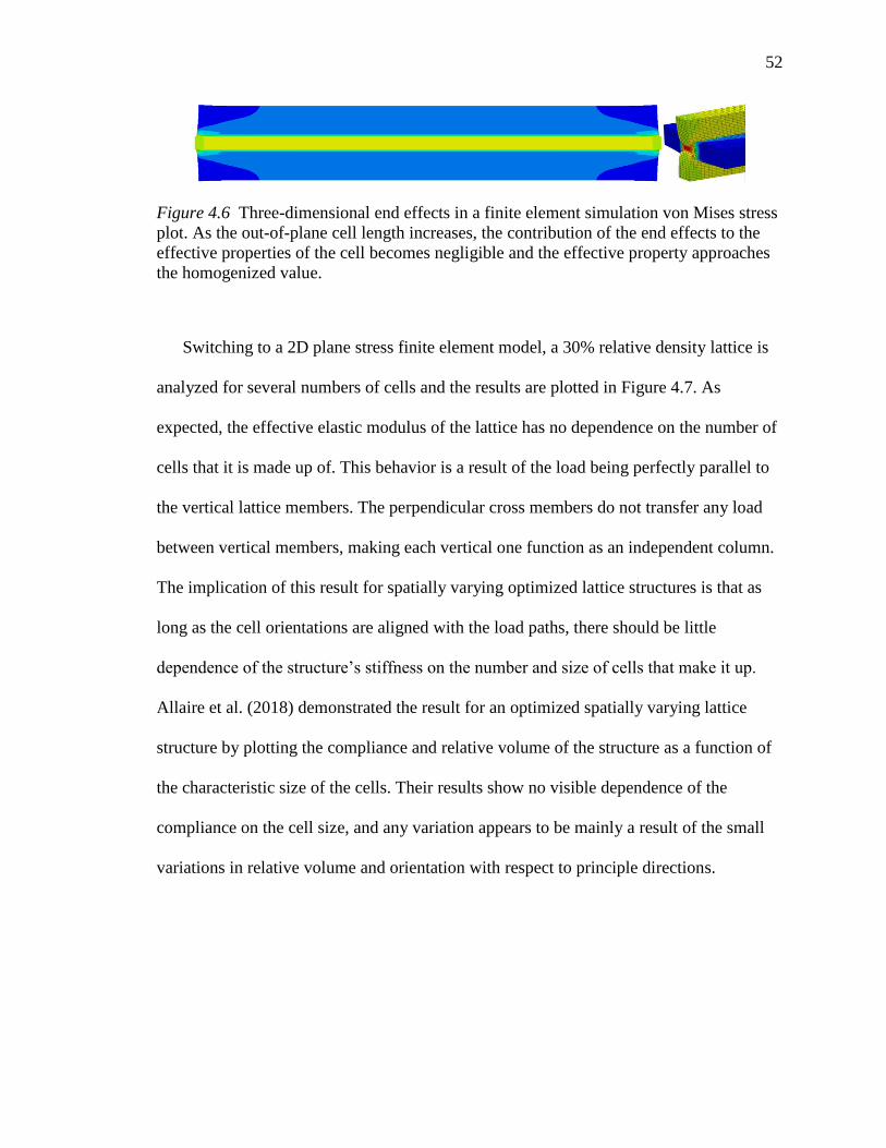
52
Figure 4.6 Three-dimensional end effects in a finite element simulation von Mises stress
plot. As the out-of-plane cell length increases, the contribution of the end effects to the
effective properties of the cell becomes negligible and the effective property approaches
the homogenized value.
Switching to a 2D plane stress finite element model, a 30% relative density lattice is
analyzed for several numbers of cells and the results are plotted in Figure 4.7. As
expected, the effective elastic modulus of the lattice has no dependence on the number of
cells that it is made up of. This behavior is a result of the load being perfectly parallel to
the vertical lattice members. The perpendicular cross members do not transfer any load
between vertical members, making each vertical one function as an independent column.
The implication of this result for spatially varying optimized lattice structures is that as
long as the cell orientations are aligned with the load paths, there should be little
dependence of the structure’s stiffness on the number and size of cells that make it up.
Allaire et al. (2018) demonstrated the result for an optimized spatially varying lattice
structure by plotting the compliance and relative volume of the structure as a function of
the characteristic size of the cells. Their results show no visible dependence of the
compliance on the cell size, and any variation appears to be mainly a result of the small
variations in relative volume and orientation with respect to principle directions.

53
Figure 4.7 Effective Young’s modulus in the 1 direction versus the number of cells
making up the structure, where the homogenized value is shown by the solid black
horizontal line.
However, when the lattice is loaded diagonally, the effective Young’s modulus
shows a dependence on the number of cells due to diagonal struts transferring load
across and influencing their neighbors. For this loading case, 50% and 70% relative
densities were also investigated. Figure 4.8 shows the effective Young’s modulus for
30%, 50%, and 70% relative densities, normalized with respect to each of their
respective homogenized values, versus the number of cells in the lattice. The trend is
that the higher the relative density, the less cells that are needed to have an effective
stiffness close to that of the homogenized value. 30% density falls within 1% error of
its homogenized value with eight cells per side, 50% density achieves this with seven
cells, and 70% density requires only five cells. For cells which cannot be aligned such
that their members are tangential to the load paths (e.g. a hexagonal honeycomb cell
which always has bending dominated deformations), it is expected that the number of
cells making up the structure will always affect the overall properties of that structure.

54
Figure 4.8 Normalized effective Young’s moduli when loaded at a 45 degree angle for
30%, 50%, and 70% relative densities versus the number of cells in the structure. The
normalized homogenized values of each density are shown by the solid black horizontal
line.
4.5. Effect of Relative Density on Young’s Modulus
Plotting the analytical equation for Young’s modulus as a function of relative density
with Equation (58) along with the values obtained using homogenization results in Figure
4.9. The analytical equation matches the homogenization results well at low relative
densities. At higher relative densities, the homogenization deviates from the analytical
results. This can be explained by the fact that the analytical derivation does not include
the contribution of the cross member to the stiffness of the structure. When the vertical
members are compressed, the cross members are squeezed where they connect to the
vertical members. This adds extra stiffness to the structure, and this effect becomes more
pronounced with thicker cross members.

55
Figure 4.9 Young’s modulus versus relative density for a 30% relative density lattice.
A finite element analysis of the cell in compression in Figure 4.10 shows this effect
clearly. At 100% relative density, the cell becomes a solid block of material, and so the
analytical equation is able to predict the stiffness accurately again (it is simply the
Young’s modulus of the solid material). The plane strain homogenized stiffness is larger
than plane stress and 3D due to the additional resistance created by the plane strain
condition and the Poisson effect.
Figure 4.10 Von Mises stress contour plot and deformation of a lattice cell under a
compression displacement in the vertical direction. The deformation of the horizontal
member contributes to the effective stiffness of the lattice.

56
4.6. Effect of the Number of Cells on Buckling Load
For buckling analysis using FEA, an additional node at the top surface of the finite
element model is constrained in the lateral direction to create fixed-fixed boundary
conditions that would be seen in a standard compression experiment using flat plates. The
analysis is repeated for a 30% relative density lattice using varying numbers of cells and
the results are plotted in Figure 4.11 along with examples of the mode shapes. Unlike the
effective Young’s modulus when loaded parallel to the cell walls, the effective buckling
stress, computed using linear static buckling analysis, shows a dependence on the number
of cells making up the lattice. It converges to an asymptote value at approximately 8x8
cells. The effective buckling stress is highest with only one cell and reduces as more cells
are added. The relative densities are kept unchanged while the number of cells increases,
which results in a lower buckling load by increasing the slenderness ratio of the vertical
members.
Figure 4.11 Effective buckling stress and mode shapes of a 30% relative density lattice
versus number of cells in the structure.

57
4.7. Effect of Relative Density on Buckling Load and Failure Mode
Using the properties of the material used for manufacturing test specimens,
Equation (63) can be used to predict a critical density where the failure mode under
compression loading changes from purely elastic buckling to plastic buckling. Since
the members of the lattice bend when the structure buckles, the average of the yield
strength in compression and tension is used (29 MPa). Plotting the analytical yield
load versus relative density with the buckling load from FEA shows the critical point
as the intersection of the two curves. Also plotting the analytical equation for
buckling stress, it can be closely matched to the FEA results by setting 𝑛 = 0.85.
This is shown in Figure 4.12.
Figure 4.12 Effective failure stresses versus relative density for an 8x8 lattice structure.
The intersection of the buckling stress curve and yield stress curve represents the critical
density.
58
Wang and McDowell (2004) stated that 𝑛 ≈ 1, but by matching to FEA results a
more precise value of 0.85 can be determined. Based on this analysis, the critical
relative density for the square cell with square hole structure under fixed-fixed
boundary conditions is (𝜌∗ 𝜌𝑠⁄ )𝑐𝑟𝑖𝑡𝑖𝑐𝑎𝑙 ≈ 0.4. Below this density and the structure may
elastically buckle under compression loading.

59
5. Lattice Structures: Experimental Analysis
To verify the numerical analysis of the previous section, lattice structures were also
additively manufactured and experimentally tested. First, basic lattice structures made of
tiled unit cells were tested to investigate their stiffness, strength, and buckling behavior at
different relative densities. Several examples of complex spatially varying lattice
structures are also tested and analyzed to demonstrate the advantages of using
metamaterials, or microstructures, to build macrostructures.
5.1. Additive Manufacturing Process and Material Properties
Several different additive manufacturing processes were considered for creating
physical test specimens. Fused deposition modeling (FDM) and fused filament
fabrication (FFF) printers using acrylonitrile butadiene styrene (ABS) plastics were
investigated but were found to produce specimens with poor dimensional accuracy,
significant warpage, and anisotropic and inconsistent mechanical properties. Selective
laser sintering (SLS) processes were considered next, and Hewlett-Packard’s (HP)
Multi Jet Fusion (MJF) process was selected. MJF functions similarly to SLS but
makes use of fusing agents to aid in sintering the powders together. MJF offers high
accuracy, high density, low cost, and short lead time parts with ductile material
behavior. All test specimens in this thesis were manufactured by Autotiv
Manufacturing Corporation using HP’s MJF process with HP 3D High Reusability
PA 12, a nylon material.
All specimens were tested on an MTS Criterion Model 43 testing system using a
50 kN load cell. Digital image correlation (DIC) data was also collected using the
VIC-3D system by Correlated Solutions, Inc. to obtain images and deformation data

60
from each test. Material properties were tested following ASTM standard test methods
D638-14 and D695-15 for tensile and compressive properties of plastics. Type 1 tensile
specimens at 4mm thickness were used for measuring the tensile properties. The
rectangular prisms for strength (12.7x12.7x25.4mm3), and modulus or offset yield
(12.7x12.7x50.8mm3) were tested to obtain compressive properties. During the testing of
the taller modulus prisms, they were observed to exhibit some buckling behavior.
Without access to a support jig for thin compression specimens, the shorter strength
prism data was used for all compressive properties.
PA 12 manufactured with SLS has been previously reported to have different
properties in tension and compression by (Maskery et al., 2018) and (Ngim et al., 2009),
and this result was also found in the present study. From the compression test, there is a
linear region followed by plastic deformation. From the tension test, the curve is entirely
nonlinear with no obvious linear elastic region, although it has approximately the same
initial slope as the compression curve. The tension test also showed significantly less
strength than the compression test. Since the compression data had a clear linear elastic
portion of the stress-strain curve, it was used to obtain the elastic modulus 𝐸. Separate
yield and ultimate strength values could be obtained for tension and compression
individually. The average material properties determined from the test results are
summarized in Table 5.1.
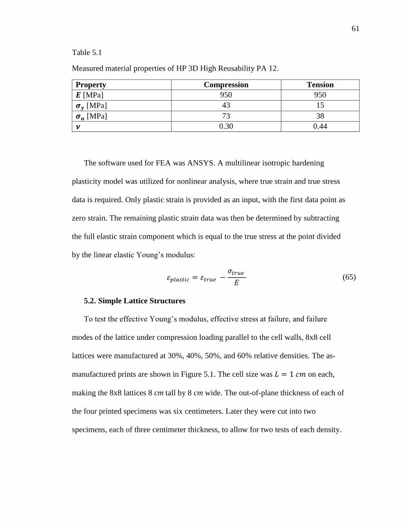
61
Table 5.1
Measured material properties of HP 3D High Reusability PA 12.
Property Compression Tension
𝑬 [MPa] 950 950
𝝈𝒚 [MPa] 43 15
𝝈𝒖 [MPa] 73 38
𝝂 0.30 0.44
The software used for FEA was ANSYS. A multilinear isotropic hardening
plasticity model was utilized for nonlinear analysis, where true strain and true stress
data is required. Only plastic strain is provided as an input, with the first data point as
zero strain. The remaining plastic strain data was then be determined by subtracting
the full elastic strain component which is equal to the true stress at the point divided
by the linear elastic Young’s modulus:
휀𝑝𝑙𝑎𝑠𝑡𝑖𝑐 = 휀𝑡𝑟𝑢𝑒 −
𝜎𝑡𝑟𝑢𝑒 𝐸
(65)
5.2. Simple Lattice Structures
To test the effective Young’s modulus, effective stress at failure, and failure
modes of the lattice under compression loading parallel to the cell walls, 8x8 cell
lattices were manufactured at 30%, 40%, 50%, and 60% relative densities. The as-
manufactured prints are shown in Figure 5.1. The cell size was 𝐿 = 1 𝑐𝑚 on each,
making the 8x8 lattices 8 cm tall by 8 cm wide. The out-of-plane thickness of each of
the four printed specimens was six centimeters. Later they were cut into two
specimens, each of three centimeter thickness, to allow for two tests of each density.
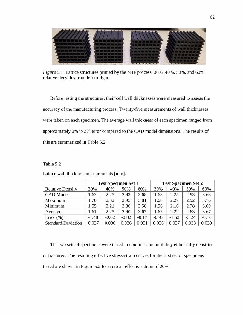
62
Figure 5.1 Lattice structures printed by the MJF process. 30%, 40%, 50%, and 60%
relative densities from left to right.
Before testing the structures, their cell wall thicknesses were measured to assess the
accuracy of the manufacturing process. Twenty-five measurements of wall thicknesses
were taken on each specimen. The average wall thickness of each specimen ranged from
approximately 0% to 3% error compared to the CAD model dimensions. The results of
this are summarized in Table 5.2.
Table 5.2
Lattice wall thickness measurements [mm].
Test Specimen Set 1 Test Specimen Set 2
Relative Density 30% 40% 50% 60% 30% 40% 50% 60%
CAD Model 1.63 2.25 2.93 3.68 1.63 2.25 2.93 3.68
Maximum 1.70 2.32 2.95 3.81 1.68 2.27 2.92 3.76
Minimum 1.55 2.21 2.86 3.58 1.56 2.16 2.78 3.60
Average 1.61 2.25 2.90 3.67 1.62 2.22 2.83 3.67
Error (%) -1.48 -0.02 -0.82 -0.17 -0.97 -1.53 -3.24 -0.10
Standard Deviation 0.037 0.030 0.026 0.051 0.036 0.027 0.038 0.039
The two sets of specimens were tested in compression until they either fully densified
or fractured. The resulting effective stress-strain curves for the first set of specimens
tested are shown in Figure 5.2 for up to an effective strain of 20%.

63
Figure 5.2 Effective stress-strain curves from compression tests on 8x8 lattice structures
of relative densities 30%, 40%, 50%, and 60%.
The 30% relative density lattice was the only one to fully densify without fracturing
after the collapse of the first layer of cells. DIC images of von Mises strains for the
relative densities of 30% and 60% before and after buckling are shown in Figure 5.3.
Figure 5.2 shows that the 30% relative density lattice has a linear effective stress-strain
curve until it fails suddenly by buckling. The 40% relative density lattice shows some
nonlinearity before it buckles, indicating that material yielding has become an important
factor, while the 50% and 60% density lattices show obvious yielding in their stress-
strain curves meaning that material yielding is dominating for relative densities this high.
Based on these experimental results, the relative density transition point where the failure
mode switches from elastic to plastic buckling is somewhere just below 40% density,
which is close to the prediction of the analysis in Section 4.7.
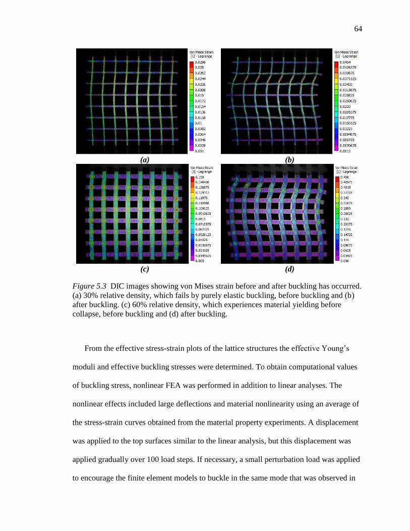
64
(a) (b)
(c) (d)
Figure 5.3 DIC images showing von Mises strain before and after buckling has occurred.
(a) 30% relative density, which fails by purely elastic buckling, before buckling and (b)
after buckling. (c) 60% relative density, which experiences material yielding before
collapse, before buckling and (d) after buckling.
From the effective stress-strain plots of the lattice structures the effective Young’s
moduli and effective buckling stresses were determined. To obtain computational values
of buckling stress, nonlinear FEA was performed in addition to linear analyses. The
nonlinear effects included large deflections and material nonlinearity using an average of
the stress-strain curves obtained from the material property experiments. A displacement
was applied to the top surfaces similar to the linear analysis, but this displacement was
applied gradually over 100 load steps. If necessary, a small perturbation load was applied
to encourage the finite element models to buckle in the same mode that was observed in
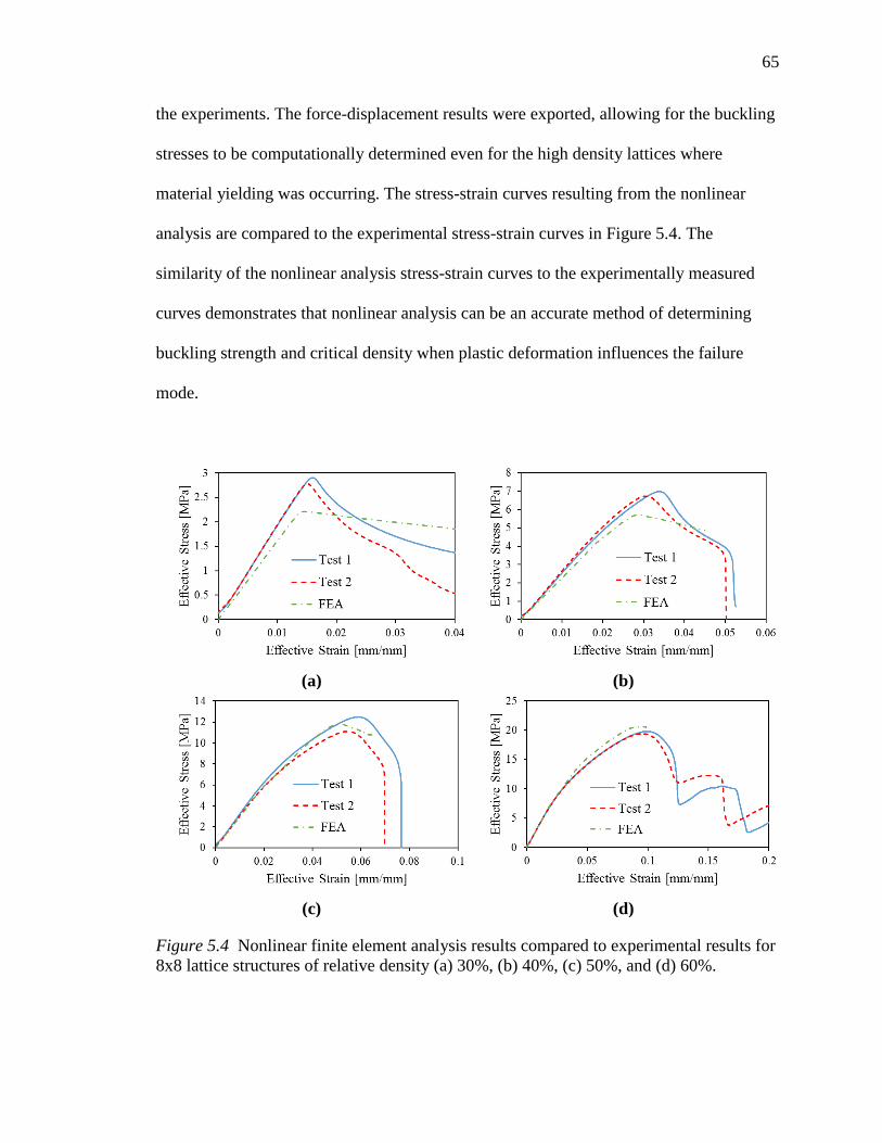
65
the experiments. The force-displacement results were exported, allowing for the buckling
stresses to be computationally determined even for the high density lattices where
material yielding was occurring. The stress-strain curves resulting from the nonlinear
analysis are compared to the experimental stress-strain curves in Figure 5.4. The
similarity of the nonlinear analysis stress-strain curves to the experimentally measured
curves demonstrates that nonlinear analysis can be an accurate method of determining
buckling strength and critical density when plastic deformation influences the failure
mode.
(a) (b)
(c) (d)
Figure 5.4 Nonlinear finite element analysis results compared to experimental results for
8x8 lattice structures of relative density (a) 30%, (b) 40%, (c) 50%, and (d) 60%.

66
Comparisons of the properties obtained from the experiments to those calculated with
the analytical equations, FEA, and homogenization are summarized in Table 5.3 and
Table 5.4. In Table 5.3 summarizing Young’s modulus results, FEA and homogenization
show excellent agreement with themselves and to the experimental results for 50% and
60% densities. For 30% and 40% densities, the stiffness obtained from FEA has errors of
around 18% and 12%, respectively. This error is attributed to variabilities in the additive
manufacturing process. While the wall thickness measurements in Table 5.2 are very
close to the CAD model dimensions, any other aspect of the manufacturing process may
have caused the higher errors for the thinner wall thickness structures. It is speculated
that this could be related to heat, as higher temperatures could build up in thinner features
where there is less material for the heat to dissipate into. Higher temperatures can create
stronger material by more thoroughly melting or sintering powder together, as
investigated by Gibson and Shi (1997) who show that fill laser power in SLS increases
the density and tensile strength of nylon material.
In Table 5.4 showing buckling stress results, analytical, linear FEA, and nonlinear
FEA are in good agreement with each other for 30% relative density. The experimental
results are higher, due to the same reasons they are for the elastic modulus. At higher
densities, the analytical and linear FEA results diverge from the experimental. This is
because material yielding reduces the buckling load below the purely elastic buckling
load. Nonlinear FEA results remain close to the experimental for the higher densities
because of its ability to include the effects of the material nonlinearity on the buckling
behavior.
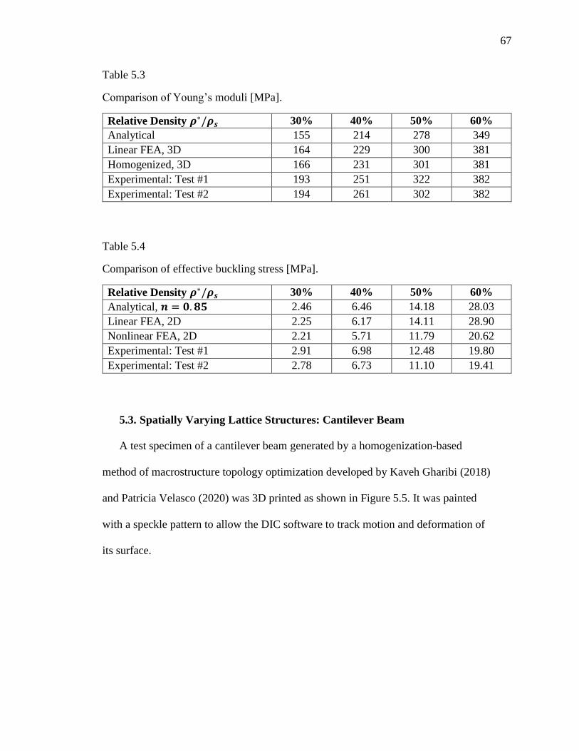
67
Table 5.3
Comparison of Young’s moduli [MPa].
Relative Density 𝝆∗/𝝆𝒔 30% 40% 50% 60%
Analytical 155 214 278 349
Linear FEA, 3D 164 229 300 381
Homogenized, 3D 166 231 301 381
Experimental: Test #1 193 251 322 382
Experimental: Test #2 194 261 302 382
Table 5.4
Comparison of effective buckling stress [MPa].
Relative Density 𝝆∗/𝝆𝒔 30% 40% 50% 60%
Analytical, 𝒏 = 𝟎. 𝟖𝟓 2.46 6.46 14.18 28.03
Linear FEA, 2D 2.25 6.17 14.11 28.90
Nonlinear FEA, 2D 2.21 5.71 11.79 20.62
Experimental: Test #1 2.91 6.98 12.48 19.80
Experimental: Test #2 2.78 6.73 11.10 19.41
5.3. Spatially Varying Lattice Structures: Cantilever Beam
A test specimen of a cantilever beam generated by a homogenization-based
method of macrostructure topology optimization developed by Kaveh Gharibi (2018)
and Patricia Velasco (2020) was 3D printed as shown in Figure 5.5. It was painted
with a speckle pattern to allow the DIC software to track motion and deformation of
its surface.

68
Figure 5.5 Optimized cantilever beam test specimen as printed by MJF.
The specimen was tested to failure in the MTS testing system at three millimeters of
displacement per minute while capturing images each second with the DIC system. The
DIC data allowed for the actual displacements and strain components everywhere on the
part to be measured and compared to FEA results. During the test the beam failed by
breaking off from its base, which was clamped inside the fixture. The failed beam is
shown in Figure 5.6.
Figure 5.6 Failure of the optimized lattice cantilever beam.

69
The deformation inside the fixture needed to be accounted for by using a full 3D
finite element representation of the test specimen and simulating the compression-only
contact between the specimen and its retaining plates. In this case, the contact simulation
could be done fairly easily by only constraining the parts of the base that would come
into compression contact with the fixture clamping system. Doing this for the
optimized beam gives a load-displacement slope that agrees with the linear portion of
the experimental results, plotted in Figure 5.7.
Figure 5.7 Force-displacement curve measured during the test of the optimized beam
compared to the slope computed using linear FEA on the three-dimensional test specimen
CAD model.
While the cantilever specimen in this experiment failed at its base with an applied
load of 1197 N, this may have been preventable with larger fillets or a better
clamping system that restrained more of the deformation inside the fixture. Also,
structures other than a cantilever beam with different support conditions may not have
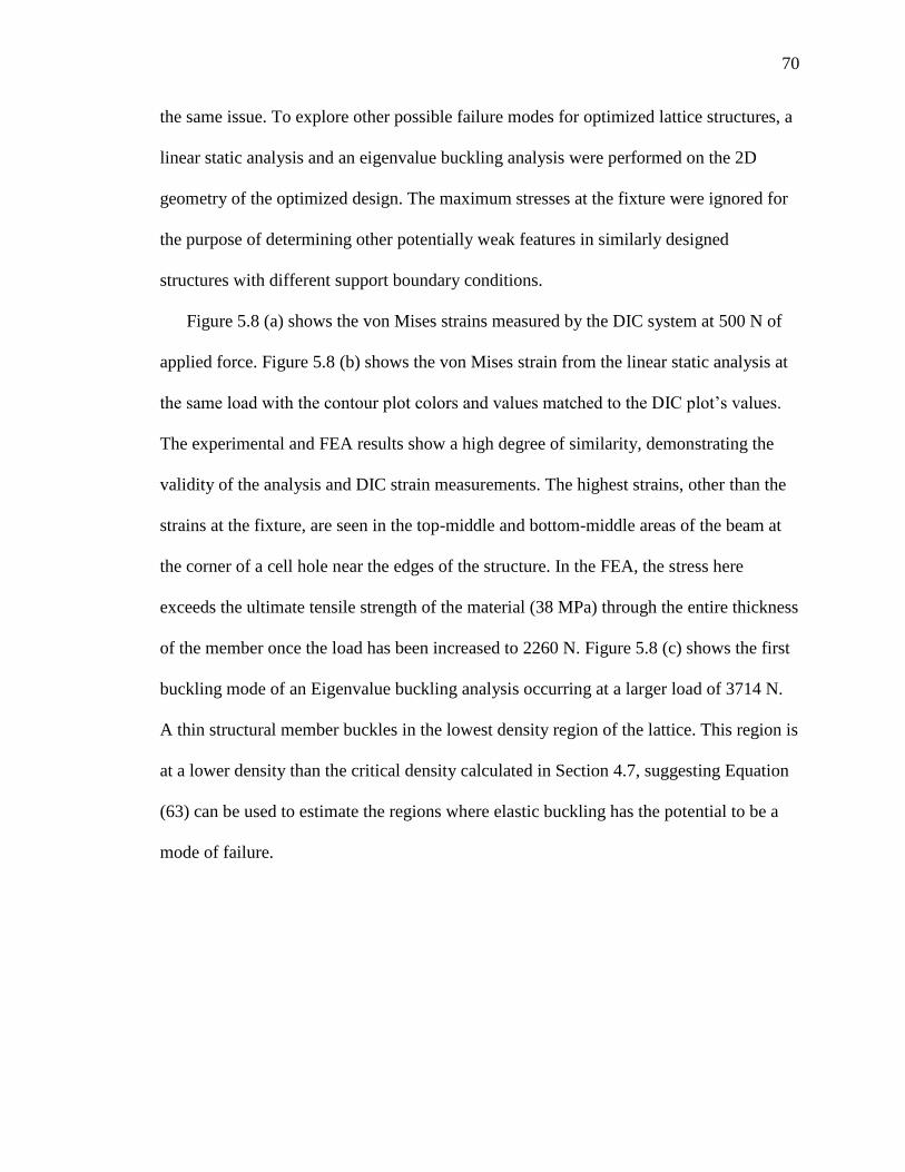
70
the same issue. To explore other possible failure modes for optimized lattice structures, a
linear static analysis and an eigenvalue buckling analysis were performed on the 2D
geometry of the optimized design. The maximum stresses at the fixture were ignored for
the purpose of determining other potentially weak features in similarly designed
structures with different support boundary conditions.
Figure 5.8 (a) shows the von Mises strains measured by the DIC system at 500 N of
applied force. Figure 5.8 (b) shows the von Mises strain from the linear static analysis at
the same load with the contour plot colors and values matched to the DIC plot’s values.
The experimental and FEA results show a high degree of similarity, demonstrating the
validity of the analysis and DIC strain measurements. The highest strains, other than the
strains at the fixture, are seen in the top-middle and bottom-middle areas of the beam at
the corner of a cell hole near the edges of the structure. In the FEA, the stress here
exceeds the ultimate tensile strength of the material (38 MPa) through the entire thickness
of the member once the load has been increased to 2260 N. Figure 5.8 (c) shows the first
buckling mode of an Eigenvalue buckling analysis occurring at a larger load of 3714 N.
A thin structural member buckles in the lowest density region of the lattice. This region is
at a lower density than the critical density calculated in Section 4.7, suggesting Equation
(63) can be used to estimate the regions where elastic buckling has the potential to be a
mode of failure.

71
(a)
(b)
(c)
Figure 5.8 (a) Von Mises strain results from DIC at a load of 500 N, (b) FEA results at
the same load with color scale values matched as closely as possible to the DIC results,
and (c) the first buckling mode shape.
Based on the computational analysis, the optimized cantilever beam design’s most
critical failure mode is fracturing at the base, which is confirmed by the experiment. This
point of failure is difficult to remedy for a cantilever beam, although other kinds of
72
structures such as simply supported beams may not have such severe stresses at their
supports. In these cases, the structure may fail by a different mechanism. In the cantilever
beam studied here, the next potential weak point is the high stress present in the top-
middle and bottom-middle sections. This was likely created by placing a cell hole corner
near the structure’s edge, creating a thinner point in the member with higher stress which
is also exacerbated by the sharp corner of the rectangular hole. A cell geometry using a
hole with rounded corners may also help to relieve this stress, and if that issue could be
solved, then elastic buckling of lattice cell walls in low relative density regions would
become the next likely failure mode.
5.4. Spatially Varying Lattice Structures: Three-Point Bending
Experimental testing was also performed on three-point bending structures designed
using conventional SIMP topology optimization and the methods of (Velasco, 2020) with
triangular lattice material. Each beam was generated in a 3:1 aspect ratio rectangular
design space, with two load cases of a point load near the left and right sides on the top of
the beam. The final designs were scaled to a height of 62 millimeters with an out-of-plane
thickness of 15 millimeters. Since the final designs can have different relative volumes
than the optimization constraint, the slope of the force-displacement curve per unit
surface area of the front face is used as a performance indicator to compare different
designs. For a linear force-displacement relationship this is:
𝑆𝑝𝑒𝑐𝑖𝑓𝑖𝑐 𝑆𝑡𝑖𝑓𝑓𝑛𝑒𝑠𝑠 =
𝑃
𝛿𝐴 (66)
Where 𝑃 is the applied load, 𝛿 is the deflection at the point of load application, and 𝐴
is the area of the front face of the structure. The computational results are displayed in
Table 5.5, showing that the specific stiffness of the triangular lattice design, Case 1,
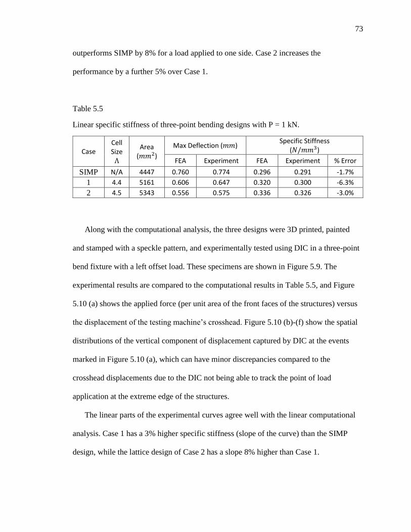
73
outperforms SIMP by 8% for a load applied to one side. Case 2 increases the
performance by a further 5% over Case 1.
Table 5.5
Linear specific stiffness of three-point bending designs with P = 1 kN.
Case Cell Size Λ
Area (𝑚𝑚2)
Max Deflection (𝑚𝑚) Specific Stiffness
(𝑁/𝑚𝑚3)
FEA Experiment FEA Experiment % Error
SIMP N/A 4447 0.760 0.774 0.296 0.291 -1.7%
1 4.4 5161 0.606 0.647 0.320 0.300 -6.3%
2 4.5 5343 0.556 0.575 0.336 0.326 -3.0%
Along with the computational analysis, the three designs were 3D printed, painted
and stamped with a speckle pattern, and experimentally tested using DIC in a three-point
bend fixture with a left offset load. These specimens are shown in Figure 5.9. The
experimental results are compared to the computational results in Table 5.5, and Figure
5.10 (a) shows the applied force (per unit area of the front faces of the structures) versus
the displacement of the testing machine’s crosshead. Figure 5.10 (b)-(f) show the spatial
distributions of the vertical component of displacement captured by DIC at the events
marked in Figure 5.10 (a), which can have minor discrepancies compared to the
crosshead displacements due to the DIC not being able to track the point of load
application at the extreme edge of the structures.
The linear parts of the experimental curves agree well with the linear computational
analysis. Case 1 has a 3% higher specific stiffness (slope of the curve) than the SIMP
design, while the lattice design of Case 2 has a slope 8% higher than Case 1.

74
Interestingly, in the nonlinear range at large displacements the lattice designs show a
major strength advantage over the SIMP structure. The SIMP beam loses stiffness early
on when its comparatively few and large structural members deform significantly and
lose their ability to efficiently transfer load to the supports. It reaches a maximum load of
4370 Newtons before failing catastrophically at a crosshead displacement of 8.9
millimeters in Figure 5.10 (b).
(a)
(b)
(c)
Figure 5.9 Three-point bending test specimens as printed by MJF and after testing to
failure. (a) SIMP, (b) triangular lattice (Case 1), (c) triangular lattice (Case 2).
The triangular lattice beam of Case 1 continues to carry larger loads well beyond the
strength of the SIMP design, reaching a maximum of 7934 Newtons for a 57%
improvement to peak load per unit area. Its many small and closely spaced lattice
members provide redundant load paths that the SIMP design does not have, allowing it to

75
achieve much higher deflections and forces by redistributing internal loads as individual
small members reach their limits. An easily observable example of this load path
redundancy is point (c) of the load-displacement curve, where a single small strut
fractures in Figure 5.10 (c), but the overall structure continues to carry increasing loads.
Following this strut fracture, a different region of lattice material buckles at 9.5
millimeters of crosshead displacement, but the beam is able to continue deforming up
until 10.2 millimeters at point (d) in Figure 5.10 (d) before failing completely.
The triangular lattice beam of Case 2 similarly experiences much higher strength than
the SIMP equivalent, as well as a progressive failure. Figure 5.10 (e) shows the structure
at 8 millimeters of crosshead displacement after an initial local buckling event. Following
this, it continues to deform while carrying a load per unit area approximately 35% larger
than the SIMP beam’s maximum. Two small members fracture at 9.2 millimeters of
crosshead displacement, Figure 5.10 (f), and then complete failure occurs at 9.9
millimeters.
The results of these experiments conclude that optimization based on lattice structures
can produce designs with higher linear stiffness than conventional SIMP topology
optimization. Additionally, the stiffness and strength was shown to be up to 57% greater
than SIMP at large displacements due to the robust nature and progressive failure
behavior of the triangular lattice cells.
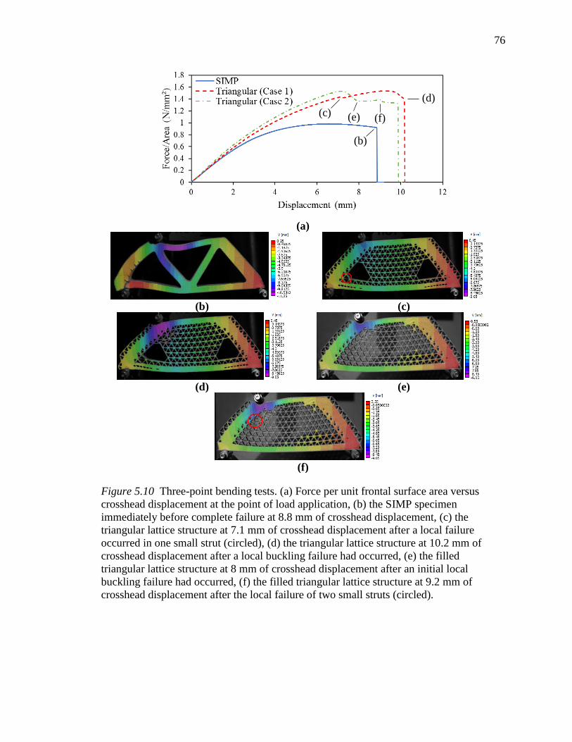
76
(a)
(b) (c)
(d) (e)
(f)
Figure 5.10 Three-point bending tests. (a) Force per unit frontal surface area versus
crosshead displacement at the point of load application, (b) the SIMP specimen
immediately before complete failure at 8.8 mm of crosshead displacement, (c) the
triangular lattice structure at 7.1 mm of crosshead displacement after a local failure
occurred in one small strut (circled), (d) the triangular lattice structure at 10.2 mm of
crosshead displacement after a local buckling failure had occurred, (e) the filled
triangular lattice structure at 8 mm of crosshead displacement after an initial local
buckling failure had occurred, (f) the filled triangular lattice structure at 9.2 mm of
crosshead displacement after the local failure of two small struts (circled).
(c) (e) (f)
(b)
(d)

77
6. Conclusions
This thesis presented a stress-based and robust topology optimization framework for
mechanical and thermoelastic microstructures constructed from up to two different
materials and a void phase. The methods were developed to take advantage of multi-
material metal additive manufacturing technology and provide a tool for designing
practical and reliable thermal structures for use in demanding applications. A formulation
based on homogenization theory for mechanical and thermal stress analysis was
developed, allowing for loads to be defined as macroscopic stresses, macroscopic strains,
and uniform thermal loads. A method of worst-case stress analysis was then included,
which allowed for effective stress-based optimizations with complete uncertainty in
loading conditions. The adjoint sensitivity analysis for each stress method was presented
for use in gradient-based optimization problems, and a method for consideration of
uniform manufacturing uncertainties was included which was motivated by the
observation that the properties of thermoelastic metamaterials are very sensitive to small
design changes brought about by the stress-based formulations.
The framework was used to generate several designs made from Invar 36 and
stainless steel 304L, including a single material microstructure with maximum stiffness,
an isotropic microstructure with zero thermal expansion and maximum bulk modulus,
and a low-stiffness microstructure with negative thermal expansion. The stress-based
formulations were applied and stresses of up to 2.7 times the allowable levels were
controlled while worst-case stresses were reduced to as low as 17% the values of the
stiffness-based designs. Comparatively small tradeoffs to thermal expansion or stiffness
properties resulted. Next, it was shown that manufacturing uncertainties could increase

78
stresses and significantly alter the thermal expansions of the stress-based designs to the
point that they were no longer negative or nowhere near the intended value of zero. The
manufacturing uncertainty method was combined with the worst-case stress method,
producing a zero thermal expansion microstructure with simplified features and a
negative thermal expansion microstructure with a significantly different layout of
materials. These microstructures were shown to be more robust with respect to load
uncertainty in both stiffness and strength, while also possessing strength and thermal
expansion properties that were less sensitive to uniform manufacturing errors.
This thesis work also investigated the mechanical properties of simple lattice
structures. First, the lattice unit cell was analyzed using numerical homogenization, finite
element, and analytical techniques to gain insight into its properties. This analysis
showed orthotropic, highly orientation-dependent stiffness and strength properties. The
effect of the number of cells used to build a macrostructure was investigated, uncovering
that the number of cells in a lattice structure with square holes has no effect on structural
stiffness when the cell members are aligned to the load direction. If cells are not aligned
to the loads, about 5-10 cells on each axis (25-100 cells in the structure), depending on
the relative density, are necessary for stiffness to be at a maximum and properties
obtained using homogenization theory to be valid.
The effect of the relative density was also investigated, verifying an analytical
equation for critical buckling density and showing that linear buckling analysis is only
valid for relative densities below about 40% for the boundary conditions and material
used in this study. At relative densities above the critical density, material nonlinearity
became an important factor and nonlinear finite element analysis was shown to give
79
accurate failure stress results. Compression test experiments were performed on four
different relative densities of an 8x8 cell lattice configuration additively manufactured
using multi-jet fusion, verifying the analysis results and demonstrating the accuracies and
deficiencies of the various analysis methods.
Test specimens of spatially varying lattice structures were also additively
manufactured using multi-jet fusion and experimentally tested to failure. The cantilever
beam test showed that stress concentrations at the sharp corners of the basic lattice cell
holes could be a cause of failure, as well as that lattice cells in regions of low relative
density have the possibility of failing by elastic buckling. Nevertheless, lattice structures
were shown to create superior performance in macrostructures compared to SIMP
topology optimization in the tests of three-point bending beams. Both higher stiffness and
significantly improved ultimate strength were attained due to the redundant load paths
created by the lattices.
For future work, the stress-based and robust metamaterial topology optimization
method developed in Sections 2 and 3 can be utilized to design optimized periodic
microstructures with greater stiffness and strength properties than the basic lattice
structures analyzed in Sections 4 and 5. These optimized microstructures can then be
used to design even higher performance macrostructures, potentially leading to
improvements in many structural applications by saving weight, saving materials, or by
tailoring macroscopic properties to achieve special mechanical and thermal properties.

80
REFERENCES
Allaire, G., Geoffroy-Donders, P., & Pantz, O. (2018). Topology optimization of
modulated and oriented periodic microstructures by the homogenization method.
Computers & Mathematics with Applications.
Allaire, G., Geoffroy-Donders, P., & Pantz, O. (2019). Topology optimization of
modulated and oriented periodic microstructures by the homogenization method.
Computers & Mathematics with Applications, 78(7), 2197-2229.
Andreassen, E., & Andreasen, C. S. (2014). How to determine composite material
properties using numerical homogenization. Computational Materials Science,
83, 488-495.
Andreassen, E., Clausen, A., Schevenels, M., Lazarov, B. S., & Sigmund, O. (2011).
Efficient topology optimization in MATLAB using 88 lines of code. Structural
and Multidisciplinary Optimization, 43(1), 1-16.
Andreassen, E., Lazarov, B. S., & Sigmund, O. (2014). Design of manufacturable 3D
extremal elastic microstructure. Mechanics of Materials, 69(1), 1-10.
Bandyopadhyay, A., & Heer, B. (2018). Additive manufacturing of multi-material
structures. Materials Science and Engineering: R: Reports, 129, 1-16.
Bendsoe, M. P., & Sigmund, O. (2013). Topology optimization: theory, methods, and
applications: Springer Science & Business Media.
Bruggi, M. (2008). On an alternative approach to stress constraints relaxation in topology
optimization. Structural and Multidisciplinary Optimization, 36(2), 125-141.
Bruggi, M., & Corigliano, A. (2019). Optimal 2D auxetic micro-structures with band gap.
Meccanica, 54(13), 2001-2027.
Bruns, T. E., & Tortorelli, D. A. (2001). Topology optimization of non-linear elastic
structures and compliant mechanisms. Computer Methods in Applied Mechanics
and Engineering, 190(26-27), 3443-3459.
Coelho, P. G., Guedes, J. M., & Cardoso, J. B. (2019). Topology optimization of cellular
materials with periodic microstructure under stress constraints. Structural and
Multidisciplinary Optimization, 59(2), 633-645.
Collet, M., Noël, L., Bruggi, M., & Duysinx, P. (2018). Topology optimization for
microstructural design under stress constraints. Structural and Multidisciplinary
Optimization, 58(6), 2677-2695.
81
da Silva, G. A., Beck, A. T., & Sigmund, O. (2019). Stress-constrained topology
optimization considering uniform manufacturing uncertainties. Computer
Methods in Applied Mechanics and Engineering, 344, 512-537.
Deaton, J. D., & Grandhi, R. V. (2014). A survey of structural and multidisciplinary
continuum topology optimization: post 2000. Structural and Multidisciplinary
Optimization, 49(1), 1-38.
Deaton, J. D., & Grandhi, R. V. (2016). Stress-based design of thermal structures via
topology optimization. Structural and Multidisciplinary Optimization, 53(2), 253-
270.
Dong, G., Tang, Y., & Zhao, Y. F. (2019). A 149 Line Homogenization Code for Three-
Dimensional Cellular Materials Written in MATLAB. Journal of Engineering
Materials and Technology, 141(1), 011005.
Duysinx, P., & Bendsøe, M. P. (1998). Topology optimization of continuum structures
with local stress constraints. International Journal for Numerical Methods in
Engineering, 43(8), 1453-1478.
Duysinx, P., & Sigmund, O. (1998). New developments in handling stress constraints in
optimal material distribution. Paper presented at the 7th
AIAA/USAF/NASA/ISSMO symposium on multidisciplinary analysis and
optimization.
Faure, A., Michailidis, G., Parry, G., Vermaak, N., & Estevez, R. (2017). Design of
thermoelastic multi-material structures with graded interfaces using topology
optimization. Structural and Multidisciplinary Optimization, 56(4), 823-837.
Geoffroy-Donders, P., Allaire, G., & Pantz, O. (2020). 3-d topology optimization of
modulated and oriented periodic microstructures by the homogenization method.
Journal of Computational Physics, 401, 108994.
Gharibi, K. (2018). Topology Optimization Using Load Path and Homogenization:
Embry-Riddle Aeronautical University.
Gibiansky, L., & Torquato, S. (1997). Thermal expansion of isotropic multiphase
composites and polycrystals. Journal of the Mechanics and Physics of Solids,
45(7), 1223-1252.
Gibson, I., & Shi, D. (1997). Material properties and fabrication parameters in selective
laser sintering process. Rapid prototyping journal, 3(4), 129-136.
Gibson, L. J., & Ashby, M. F. (1999). Cellular solids: structure and properties:
Cambridge university press.

82
Groen, J. P., & Sigmund, O. (2018). Homogenization-based topology optimization for
high-resolution manufacturable microstructures. International Journal for
Numerical Methods in Engineering, 113(8), 1148-1163.
Guedes, J., & Kikuchi, N. (1990). Preprocessing and postprocessing for materials based
on the homogenization method with adaptive finite element methods. Computer
Methods in Applied Mechanics and Engineering, 83(2), 143-198.
Guo, X., Zhao, X., Zhang, W., Yan, J., & Sun, G. (2015). Multi-scale robust design and
optimization considering load uncertainties. Computer Methods in Applied
Mechanics and Engineering, 283, 994-1009.
Hashin, Z., & Shtrikman, S. (1963). A variational approach to the theory of the elastic
behaviour of multiphase materials. Journal of the Mechanics and Physics of
Solids, 11(2), 127-140.
Hassani, B., & Hinton, E. (1998). A review of homogenization and topology optimization
I—homogenization theory for media with periodic structure. Computers &
Structures, 69(6), 707-717.
Hofmann, D. C., Kolodziejska, J., Roberts, S., Otis, R., Dillon, R. P., Suh, J.-O., . . .
Borgonia, J.-P. (2014). Compositionally graded metals: A new frontier of additive
manufacturing. Journal of Materials Research, 29(17), 1899-1910.
Hofmann, D. C., Roberts, S., Otis, R., Kolodziejska, J., Dillon, R. P., Suh, J.-o., . . .
Borgonia, J.-P. (2014). Developing gradient metal alloys through radial
deposition additive manufacturing. Scientific reports, 4, 5357.
Hollister, S. J., & Kikuchi, N. (1992). A comparison of homogenization and standard
mechanics analyses for periodic porous composites. Computational Mechanics,
10(2), 73-95.
Holmberg, E., Torstenfelt, B., & Klarbring, A. (2013). Stress constrained topology
optimization. Structural and Multidisciplinary Optimization, 48(1), 33-47.
International, A. (2015). ASTM D638-14, Standard Test Method for Tensile Properties of
Plastics: ASTM International.
Jones, R. M. (2014). Mechanics of composite materials: CRC press.
Kang, D., Park, S., Son, Y., Yeon, S., Kim, S. H., & Kim, I. (2019). Multi-lattice inner
structures for high-strength and light-weight in metal selective laser melting
process. Materials & Design, 175, 107786.
83
Kazemi, H., Vaziri, A., & Norato, J. A. (2020). Multi-material topology optimization of
lattice structures using geometry projection. Computer Methods in Applied
Mechanics and Engineering, 363, 112895.
Le, C., Norato, J., Bruns, T., Ha, C., & Tortorelli, D. (2010). Stress-based topology
optimization for continua. Structural and Multidisciplinary Optimization, 41(4),
605-620.
Lee, E., James, K. A., & Martins, J. R. (2012). Stress-constrained topology optimization
with design-dependent loading. Structural and Multidisciplinary Optimization,
46(5), 647-661.
Maharaj, Y., & James, K. A. (2019). Metamaterial topology optimization of
nonpneumatic tires with stress and buckling constraints. International Journal for
Numerical Methods in Engineering.
Maskery, I., Aboulkhair, N. T., Aremu, A., Tuck, C., & Ashcroft, I. (2017). Compressive
failure modes and energy absorption in additively manufactured double gyroid
lattices. Additive Manufacturing, 16, 24-29.
Maskery, I., Sturm, L., Aremu, A., Panesar, A., Williams, C., Tuck, C., . . . Hague, R. J.
(2018). Insights into the mechanical properties of several triply periodic minimal
surface lattice structures made by polymer additive manufacturing. Polymer, 152,
62-71.
Ngim, D., Liu, J.-S., & Soar, R. (2009). Design optimization of consolidated granular-
solid polymer prismatic beam using metamorphic development. International
Journal of Solids and Structures, 46(3-4), 726-740.
Niu, J., Choo, H. L., Sun, W., & Mok, S. H. (2018). Analytical Solution and
Experimental Study of Effective Young's Modulus of Selective Laser Melting-
Fabricated Lattice Structure With Triangular Unit Cells. Journal of
Manufacturing Science and Engineering, 140(9), 091008.
Noël, L., & Duysinx, P. (2017). Shape optimization of microstructural designs subject to
local stress constraints within an XFEM-level set framework. Structural and
Multidisciplinary Optimization, 55(6), 2323-2338.
Osanov, M., & Guest, J. K. (2016). Topology optimization for architected materials
design. Annual Review of Materials Research, 46, 211-233.
Panetta, J., Rahimian, A., & Zorin, D. (2017). Worst-case stress relief for
microstructures. ACM Transactions on Graphics (TOG), 36(4), 1-16.
84
Picelli, R., Sivapuram, R., Townsend, S., & Kim, H. A. (2017). Stress topology
optimisation for architected material using the level set method. Paper presented
at the World Congress of Structural and Multidisciplinary Optimisation.
Sigmund, O. (1994). Materials with prescribed constitutive parameters: an inverse
homogenization problem. International Journal of Solids and Structures, 31(17),
2313-2329.
Sigmund, O. (1995). Tailoring materials with prescribed elastic properties. Mechanics of
Materials, 20(4), 351-368.
Sigmund, O. (2000). A new class of extremal composites. Journal of the Mechanics and
Physics of Solids, 48(2), 397-428.
Sigmund, O. (2009). Manufacturing tolerant topology optimization. Acta Mechanica
Sinica, 25(2), 227-239.
Sigmund, O., & Torquato, S. (1997). Design of materials with extreme thermal expansion
using a three-phase topology optimization method. Journal of the Mechanics and
Physics of Solids, 45(6), 1037-1067.
Standard, A. (2015). D695-15. Standard test method for compressive properties of rigid
plastics.
Stolpe, M., & Svanberg, K. (2001). An alternative interpolation scheme for minimum
compliance topology optimization. Structural and Multidisciplinary Optimization,
22(2), 116-124.
Svanberg, K. (2002). A class of globally convergent optimization methods based on
conservative convex separable approximations. SIAM journal on optimization,
12(2), 555-573.
Takezawa, A., & Kobashi, M. (2017). Design methodology for porous composites with
tunable thermal expansion produced by multi-material topology optimization and
additive manufacturing. Composites Part B: Engineering, 131, 21-29.
Velasco, P. (2020). MACROSCALE PROJECTION AND MANUFACTURABILITY OF
ORIENTED HOMOGENIZED MICROSTRUCTURES: Embry-Riddle
Aeronautical University.
Vogiatzis, P., Chen, S., Wang, X., Li, T., & Wang, L. (2017). Topology optimization of
multi-material negative Poisson’s ratio metamaterials using a reconciled level set
method. Computer-Aided Design, 83, 15-32.

85
Wang, A.-J., & McDowell, D. (2004). In-plane stiffness and yield strength of periodic
metal honeycombs. Journal of engineering materials and technology, 126(2),
137-156.
Wang, F., Lazarov, B. S., & Sigmund, O. (2011). On projection methods, convergence
and robust formulations in topology optimization. Structural and
Multidisciplinary Optimization, 43(6), 767-784.
Wang, Y., Gao, J., Luo, Z., Brown, T., & Zhang, N. (2017). Level-set topology
optimization for multimaterial and multifunctional mechanical metamaterials.
Engineering Optimization, 49(1), 22-42.
Wang, Z., Palmer, T. A., & Beese, A. M. (2016). Effect of processing parameters on
microstructure and tensile properties of austenitic stainless steel 304L made by
directed energy deposition additive manufacturing. Acta Materialia, 110, 226-
235.
Yan, C., Hao, L., Hussein, A., & Young, P. (2015). Ti–6Al–4V triply periodic minimal
surface structures for bone implants fabricated via selective laser melting. Journal
of the mechanical behavior of biomedical materials, 51, 61-73.
Zhang, H., Luo, Y., & Kang, Z. (2018). Bi-material microstructural design of chiral
auxetic metamaterials using topology optimization. Composite Structures, 195,
232-248.
Zhou, S., & Li, Q. (2008). Computational design of multi-phase microstructural materials
for extremal conductivity. Computational Materials Science, 43(3), 549-564.