TOPOLOGY OF SPACES OF MICRO-IMAGES, AND …qs397kn3896/PhD...TOPOLOGY OF SPACES OF MICRO-IMAGES, AND...
106
TOPOLOGY OF SPACES OF MICRO-IMAGES, AND AN APPLICATION TO TEXTURE DISCRIMINATION A DISSERTATION SUBMITTED TO THE DEPARTMENT OF MATHEMATICS AND THE COMMITTEE ON GRADUATE STUDIES OF STANFORD UNIVERSITY IN PARTIAL FULFILLMENT OF THE REQUIREMENTS FOR THE DEGREE OF DOCTOR OF PHILOSOPHY Jose Andres Perea Benitez May 2011
-
Upload
truongxuyen -
Category
Documents
-
view
216 -
download
0
Transcript of TOPOLOGY OF SPACES OF MICRO-IMAGES, AND …qs397kn3896/PhD...TOPOLOGY OF SPACES OF MICRO-IMAGES, AND...

TOPOLOGY OF SPACES OF MICRO-IMAGES,
AND AN APPLICATION TO TEXTURE DISCRIMINATION
A DISSERTATION
SUBMITTED TO THE DEPARTMENT OF MATHEMATICS
AND THE COMMITTEE ON GRADUATE STUDIES
OF STANFORD UNIVERSITY
IN PARTIAL FULFILLMENT OF THE REQUIREMENTS
FOR THE DEGREE OF
DOCTOR OF PHILOSOPHY
Jose Andres Perea Benitez
May 2011

http://creativecommons.org/licenses/by-nc/3.0/us/
This dissertation is online at: http://purl.stanford.edu/qs397kn3896
© 2011 by Jose Andres Perea Benitez. All Rights Reserved.
Re-distributed by Stanford University under license with the author.
This work is licensed under a Creative Commons Attribution-Noncommercial 3.0 United States License.
ii

I certify that I have read this dissertation and that, in my opinion, it is fully adequatein scope and quality as a dissertation for the degree of Doctor of Philosophy.
Gunnar Carlsson, Primary Adviser
I certify that I have read this dissertation and that, in my opinion, it is fully adequatein scope and quality as a dissertation for the degree of Doctor of Philosophy.
George Papanicolaou
I certify that I have read this dissertation and that, in my opinion, it is fully adequatein scope and quality as a dissertation for the degree of Doctor of Philosophy.
Andras Vasy
Approved for the Stanford University Committee on Graduate Studies.
Patricia J. Gumport, Vice Provost Graduate Education
This signature page was generated electronically upon submission of this dissertation in electronic format. An original signed hard copy of the signature page is on file inUniversity Archives.
iii

Abstract
In the paper On the Local Behavior of Spaces of Natural Images [21], the framework
of topological data analysis was used by Carlsson et al. to identify the geometric
structure of high-density regions in the state space M ⊆ S7, of 3 × 3 high-contrast
patches from natural images. The astonishing fact discovered in their work: 50%
of the points in M accumulate around a Klein bottle K, in a tubular neighborhood
occupying about 20% of the volume of S7.
Driven by this newfound model, we propose in this thesis a novel method for
representation and classification of image textures. It is shown that for any gray
scale image it is possible to project a sample of its high contrast patches onto K, and
then study the underlying probability density function
h : K −→ R
using Fourier analysis. That is, it is possible to construct a suitable orthonormal
basis B for L2(K), and describe h in terms of Fourier-like coefficients h1, . . . , hN , . . .,
which we show can be estimated with high confidence.
We then proceed on to studying the type of information contained in the estimates
[h1, . . . , hN ], and ways in which they can be used for classification purposes. We
propose several dissimilarity measures, and test these ideas on the PMTex database,
a collection of 1930 image textures which correspond to 36 different texture samples,
with instances taken under varying lightning conditions and camera viewpoint.
iv

Contents
Abstract iv
1 Introduction 1
2 Homology Inference 4
2.1 Approximation by Simplicial Complexes . . . . . . . . . . . . . . . . 5
2.2 Persistent Homology . . . . . . . . . . . . . . . . . . . . . . . . . . . 9
3 Topology of Spaces of Micro-Images 15
3.1 The Mumford Formalism . . . . . . . . . . . . . . . . . . . . . . . . . 16
3.2 Persistent Homology on M . . . . . . . . . . . . . . . . . . . . . . . 17
4 Projecting Samples Onto K 21
4.1 The Differentiable Case . . . . . . . . . . . . . . . . . . . . . . . . . . 22
4.1.1 Direction and Directionality . . . . . . . . . . . . . . . . . . . 22
4.1.2 Projection onto Cα . . . . . . . . . . . . . . . . . . . . . . . . 25
4.2 The Discrete Case . . . . . . . . . . . . . . . . . . . . . . . . . . . . . 28
4.2.1 Direction and Directionality . . . . . . . . . . . . . . . . . . . 28
4.2.2 Estimating tk . . . . . . . . . . . . . . . . . . . . . . . . . . . 34
5 A Discrete Representation 38
5.1 Coefficient Estimation in L2 . . . . . . . . . . . . . . . . . . . . . . . 39
5.2 An Orthonormal Basis for L2(K) . . . . . . . . . . . . . . . . . . . . 43
5.3 The v-Invariant . . . . . . . . . . . . . . . . . . . . . . . . . . . . . . 45
v

5.4 Preliminary Examples . . . . . . . . . . . . . . . . . . . . . . . . . . 49
6 Dissimilarity Measures 58
6.1 Naive Examples . . . . . . . . . . . . . . . . . . . . . . . . . . . . . . 58
6.2 Image Rotation . . . . . . . . . . . . . . . . . . . . . . . . . . . . . . 62
6.2.1 Behavior of the v-Invariant under the SO(2,R) action. . . . . 63
6.2.2 Computing the R-distance . . . . . . . . . . . . . . . . . . . . 67
6.2.3 A rotation invariant version of v(I) . . . . . . . . . . . . . . . 69
7 Classification Results 72
7.1 Material Categories Via Hausdorff Distance . . . . . . . . . . . . . . 73
7.2 Texture Classification From Known Instances . . . . . . . . . . . . . 77
7.3 Local to Global Information: Intrinsic distance reconstruction and
Class Partitioning . . . . . . . . . . . . . . . . . . . . . . . . . . . . . 80
8 Conclusions and Final Remarks 84
A Proof of theorem 5.2.2 86
Bibliography 93
vi

List of Tables
4.1 Estimated thresholds . . . . . . . . . . . . . . . . . . . . . . . . . . . 36
7.1 |Tp| and |Np| as functions of p . . . . . . . . . . . . . . . . . . . . . . 78
vii

List of Figures
2.1 Bar-code of noisy circle . . . . . . . . . . . . . . . . . . . . . . . . . . 13
3.1 Exemplary natural images . . . . . . . . . . . . . . . . . . . . . . . . 15
3.2 DCT basis in patch space . . . . . . . . . . . . . . . . . . . . . . . . 17
3.3 Bar-code, three circle model . . . . . . . . . . . . . . . . . . . . . . . 18
3.4 Three circle model in patch space. . . . . . . . . . . . . . . . . . . . . 18
3.5 Bar-code Klein bottle . . . . . . . . . . . . . . . . . . . . . . . . . . . 19
3.6 Klein bottle model in patch-space . . . . . . . . . . . . . . . . . . . . 19
4.1 Exemplary texture in the USC-SIPI database . . . . . . . . . . . . . 34
4.2 Direction versus directionality . . . . . . . . . . . . . . . . . . . . . . 35
4.3 Histogram of directionalities, USC Texture Database . . . . . . . . . 36
5.1 Texture of Straw . . . . . . . . . . . . . . . . . . . . . . . . . . . . . 49
5.2 v-Invariant v1(S) = (v1, . . . , vd) for Straw . . . . . . . . . . . . . . . . 49
5.3 Projected sample and heat map for Straw . . . . . . . . . . . . . . . 50
6.1 Natural multi-scale distance matrix for ensemble 2 . . . . . . . . . . . 60
6.2 Classes emerging from d4 distance on Ensemble 2 . . . . . . . . . . . 61
6.3 Evolution function ε(I) for images in Ensemble 2 . . . . . . . . . . . 62
6.4 Computational Scheme for the R-distance dR . . . . . . . . . . . . . . 69
7.1 Sample materials, PMTex database. . . . . . . . . . . . . . . . . . . . 72
7.2 Instances of a sample in the PMTex database . . . . . . . . . . . . . 73
7.3 Subspace distance matrices . . . . . . . . . . . . . . . . . . . . . . . . 74
viii

7.4 Distance matrix representing (V, dR) . . . . . . . . . . . . . . . . . . 75
7.5 Material categorization from Hausdorff distance. . . . . . . . . . . . . 76
7.6 Complete-linkage dendrogram for dM . . . . . . . . . . . . . . . . . . 77
7.7 Classification success d4, dR and d4 . . . . . . . . . . . . . . . . . . . 79
7.8 Intrinsic distance estimated from dR . . . . . . . . . . . . . . . . . . . 82
ix

Chapter 1
Introduction
The application of topological methods to the analysis of data has produced in the
last decade an increasing number of success stories. In neuroscience for instance [24],
data collected from electrodes in the visual cortex was analyzed using the theory of
persistent homology. In this framework, it was shown that homological signatures
(Betti numbers) are powerful enough to distinguish between states of visual stimuli.
In medicine, simplicial complexes for data reduction and visualization [23], duplicated
almost effortlessly results of Reaven and Miller [43] on the onsets of diabetes.
Topological tools have also been employed in computer vision with surprising
results [21]: Non-orientable surfaces appear naturally as the state space of relevant
micro-images extracted from photographs of natural scenes (natural images). The
geometric structure of these spaces lies at the center of the ideas presented in this
work, and gives two elements of novelty to our approach: The continuous character
of the texton dictionary, in contrast with the quantized nature of its predecessors
[6, 7, 38]; and the meaningfulness of the space K inside the set of all high contrast
patches from natural images.
We believe one of the major contributions of this thesis, lies in the reinterpretation
we give to the concept of texton dictionary. As seen in the work of Varma and
Zisserman [38], one of the most successful approaches in material discrimination from
image textures, consists in learning a finite collection of frequently occurring patches
from each material class in a given image database, and then agglomerating them
1

CHAPTER 1. INTRODUCTION 2
(over all classes) to form the texton dictionary. Some drawbacks are inherent to this
philosophy: The resulting code book is database dependent, and given its quantized
nature, important information might get lost when trying to associate an element in
the dictionary to a patch in an image.
With the Klein bottle, we show that it is possible to construct code books which are
both infinite, and of a continuous nature, but with a simple geometry and low intrinsic
dimension. Moreover, this new continuous dictionary captures important properties
of textures in natural images which are not tied to an specific image data set. In this
setting, the distribution on this space of patches from a particular image, becomes an
object associated to the image itself. We believe that with this interpretation, it will
be easier to discover extensions as well as applications coming from different angles.
The organization of this thesis goes as follows: In Chapter 2, titled Homology
Inference, we give some background material in the problem of estimating the ho-
mology of a topological space from finite samples. We include several constructions,
as well as results with conditions under which the homology estimation problem can
be solved. This material is presented for both completeness, and as a motivation for
the theory of persistent homology, which we include in the second part of the chapter.
Chapter 3, Topology of Spaces of Micro-Images, summarizes the results in
the papers by Mumford et. al. [3], and Carlsson et. al. [24]. Our objective with this
chapter is to explain the way in which the Klein bottle fits as a relevant part of the
space of natural micro-images.
In Chapter 4, Projecting Samples Onto K, we provide a computational frame-
work for evaluating the closest point projection
p : T −→ K
where T is a small tubular neighborhood of the Klein bottle K.
Chapter 5, A Discrete Representation, is devoted to the problem of estimating
the Fourier-like coefficients associated to a probability density function f : K −→ R,
underlying a given projected sample of high-contrast patches. We first go over the
general theory of estimation by orthogonal series, and then construct a particular

CHAPTER 1. INTRODUCTION 3
basis for L2(K). The way we do the latter, is by noticing that K is a quotient of the
torus S1×S1, and thus Fourier analysis on S1 yields an orthonormal basis for L2(K).
We end chapter 5 with some particular examples of the computations involved.
In Chapter 6, Dissimilarity Measures, we construct several (pseudo) metrics
in the frequency domain, so that we can compare the different sets of Fourier-like
coefficients defined in chapter 5. In particular we show that image rotation has
a simple interpretation in the frequency domain, and thus it is possible to define
rotation-invariant notions of dissimilarity.
In Chapter 7, Classification Results, we show how the theoretical constructions
of the previous chapter behave in a particular texture database.
We end with Conclusions and Final Remarks in Chapter 8.
Computational Details
Computations, data processing and associated plots were generated with MATLAB
R2009b, used under the Single Machine License - Stanford Extended Set.

Chapter 2
Homology Inference
In recent years, our capability to collect data has greatly surpassed our ability to
analyze it. With data sets sitting in spaces of very large dimension, in highly-
nonlinear ways, global and qualitative information are becoming more relevant. In
short, methods which are somewhat independent form choices of metric, that can
deal with large dimensions, and are robust with respect to noise or missing points,
are in high demand. It is in this scenario that topological methods for the analysis of
data [19] are becoming relevant.
One of the driving ideas behind topological data analysis is the following: A finite
set X ⊆ Rn can be thought of as a random sample taken from a topological space
X ⊆ Rn, drawn with respect to some probability density function. The hope is then
that topological information about X can be recovered from X, and that phenomena
encoded in the data can be revealed from the topology.
Take clustering for example: Given a data set X and a notion of similarity or
distance between its points, clustering attempts to partition X into meaningful sub-
sets. This of course, can be thought of as the statistical counterpart of finding the
connected components of X, which is a topological notion. The higher-level geometric
organization of the space can also reveal important information: Holes or voids in
X, which could translate into lack of coverage in a sensor network, the presence of
cancer in medical image data, or periodic phenomena, can be detected by the rank
of the homology groups Hk(X).
4

CHAPTER 2. HOMOLOGY INFERENCE 5
In summary, the topology of X, or at least its homology, is an important object of
study and the question becomes: How do we go from X ⊆ Rn to Hk(X)? We present
now some of the answers found in the literature.
2.1 Approximation by Simplicial Complexes
The category of compact subsets of Euclidean space with positive reach, introduced
by Federer in 1959 [27], comprises most of the examples one expects to find in the
study of naturally occurring data, at least up to homotopy equivalence. Intuitively, a
compact subset of Rn has positive reach if it does not have sharp cone-like points and
examples include, but are not limited to, all smoothly embedded closed manifolds.
Definition 2.1.1. Given a compact subset K of Rn, its medial axis m(K) is the set
of points x ∈ RN having at least two closest points in K. The reach of K, rch(K), is
the distance from K to m(K).
Since local smoothing does not change the homotopy type, it follows that the
class of compact sets with positive reach is general enough for a theory of homology
inference from point cloud data. What we will see now is that in addition to generality,
compact subsets with positive reach can be reconstructed (up to deformation) from
densely enough samples.
Proposition 2.1.2. Let X ⊆ RN be a compact set with R = rch(X) > 0, and let
X ⊆ X be ε-dense. That is, for all x ∈ X there exists y ∈ X so that ‖x− y‖ < ε. If
ε < (3−√
8)R and ε+√Rε < r < R−
√Rε then
Xr =⋃x∈X
B(x, r)
deformation retracts onto X. B(x, r) denotes the open ball of radius r centered at x.
Proof. The inequalities ε +√Rε < r < R −
√Rε, which make sense given that
ε < (3−√
8)R, imply that
r < R− ε and R−√
(R− ε)2 − r2 < r − ε.

CHAPTER 2. HOMOLOGY INFERENCE 6
The result is now a consequence of Theorem 4 in [11].
It follows that the homology of X coincides with that of Xr, for r in certain range
depending on both sample density and reach. The computation of Hk(Xr,Z), on the
other hand, reduces to the problem of calculating the Smith Normal Form over a
Principal Ideal Domain. Indeed, let C(X, r) be the abstract simplicial complex on X
so that {x0, . . . , xk} ∈ C(X, r) if and only if
B(x0, r) ∩ . . . ∩B(xk, r) 6= ∅.
We refer to C(X, r) as the r-Cech complex on X. As a consequence of the Nerve
Theorem [9], and the equivalence of simplicial and singular homology [2] we have:
Theorem 2.1.3 (Cech Reconstruction). The geometric realization of the Cech
complex, |C(X, r)|, is homotopy equivalent to Xr. Thus, the simplicial homology
of C(X, r) coincides with the singular homology of X, provided X is ε-dense in X,
R = rch(X) > 0, ε < (3−√
8)R and ε+√Rε < r < R−
√Rε.
There is a large body of work dedicated to the efficient computation of simplicial
homology over Principal Ideal Domains, via the Smith Normal Form of the corre-
sponding boundary matrix [31].
The previous reconstruction theorem while encouraging, puts forward many of
the difficulties one encounters when studying point clouds coming from real world
data. Consider for instance the construction of C(X, r). Since this complex takes as
vertex set all data points, it is in general extremely large, with simplices of dimension
further exceeding even that of the ambient space. In practice, it only takes a few
thousand points to make the homology computation too expensive in terms of memory
resources. As an attempt to remedy this problem, de Silva and Carlsson introduced
the Witness Complex in [48]. The main idea behind their construction is that it is
often unnecessary to use every point in the data set as a vertex, and thus one can use
a much smaller, sparse and well distributed subset, while letting the remaining data
points guide the construction of the complex.

CHAPTER 2. HOMOLOGY INFERENCE 7
Definition 2.1.4. Let (X, d) be a metric space, and let L ⊆ X be finite. A point
w ∈ X− L is called an r-witness for σ ⊆ L if
maxl∈σ
d(w, l) ≤ r + d(w,L− σ)
The r-Witness Complex W (X, L, r) is the abstract simplicial complex on L so that
∅ 6= σ ⊆ L is a simplex if and only if every ∅ 6= τ ⊆ σ has an r-witness in X− L.
By a theorem of de Silva (Corollary 9.7 in [47]), W (X, L) = W (X, L, 0) recovers
the homotopy type of X under some density conditions for L, and of curvature for X.
Theorem 2.1.5 (Witness Reconstruction). Let X be a complete Riemannian
manifold with constant sectional curvature and injectivity radius ρX. Suppose that
L ⊆ X is ε-dense (with respect to the geodesic distance), where ε ≤ ρX/3 or ε ≤ ρX/6
if X is the sphere of dimension at least 2. Then |W (X, L)| is homotopy equivalent to
X.
It is known that for smoothly embedded curves on the plane and surfaces in
R3, |W (X, L)| is homeomorphic to X under some mild sampling conditions on L
[12, 39, 40]. Thus, the requirement of constant sectional curvature can be discarded
in low dimensions. By contrast, due to the presence of badly shaped simplices, called
slivers, such guarantees are unavailable for arbitrary smooth submanifolds of Rn with
dimension k ≥ 3. This is true, unfortunately, even under strong sampling conditions
[45]. This difficulty in higher dimensions can be overcome, as suggested in [30], using
an enriched version of the Witness Complex, where vertices are assigned weights in
order to prevent the formation of slivers.
Another important construction related to the Cech complex, is the Vietoris-Rips
complex.
Definition 2.1.6. Let (X, d) be a pseudo-metric space and let r > 0. The Vietoris-
Rips complex on X at scale r, denoted by V R(X, r), is the abstract simplicial
complex on X so that {x0, . . . , xk} ∈ V R(X, r) if and only if d(xi, xj) < r for all
0 ≤ i, j ≤ k.

CHAPTER 2. HOMOLOGY INFERENCE 8
When X ⊆ RN is finite, V R(X, r) is the largest simplicial complex having the
same 1-skeleton as C(X, r), and one can check that
V R(X, r) ⊆ C(X, 2r) ⊆ V R(X, 2r).
Optimal bounds for these inclusions, which turn out to depend on N , have been
derived by de Silva and Ghrist (Theorem 2.5 in [49]).
While the considerable size of V R(X, r) is often burdensome, this is ameliorated by
removing the ambient space from the definition of the complex. As an example of the
usefulness of this generalization, let us consider an undirected connected graph: The
minimum number of edges joining two nodes induces a metric on the vertex set, and
therefore the Vietoris-Rips complex can be used to study the higher-order geometric
organization and connectivity of the graph. Many data sets, specially those coming
from biology, can be modeled as a graph and thus the importance of the Vietoris-Rips
complex.
As observed by Jean-Claude Hausmann [29], this construction has specially nice
properties for Riemannian manifolds.
Theorem 2.1.7 (Rips Reconstruction). Let X be a Riemannian manifold with
positive injectivity radius r(X). If 0 < r ≤ r(X) then |V R(X, r)| is homotopy equiv-
alent to X. Moreover, the homotopy equivalence can be chosen to be natural with
respect to the inclusion map V R(X, r) ↪→ V R(X, r′), for r ≤ r′ ≤ r(X).
Proof. See theorem 3.5 in [29].
As a consequence of the discussion following 3.11 in the same paper, one obtains:
Proposition 2.1.8. Let X be a compact Riemannian manifold with injectivity radius
r(X), and let X ⊆ X be ε-dense for 0 < ε < 14r(X). Then for every 0 < η ≤ r(M)− 4ε,
the image of the homomorphism between k-th homology groups induced by the inclu-
sion map
V R(X, 2ε+ η) ↪→ V R(X, 4ε+ η)
is isomorphic to Hk(X,Z).
CHAPTER 2. HOMOLOGY INFERENCE 9
We have summarized in this section a number of constructions which allow one
to recover the homotopy/homology type, of a class of topological spaces underlying
a given point cloud X (Cech, Witness and Rips reconstruction Theorems). These
guarantees however, depend on several sampling conditions, regularity assumptions
and good parameter choices which in reality cannot be checked. Thus the need for
theorems of statistical nature, and invariants which are free from parameter choices.
On the statistical front, interesting results have appeared regarding the estimation
of Betti numbers from random samples [42], and the study of the topology of random
simplicial complexes [35]. With respect to parameter choices (e.g. r in the definition of
C and V R), proposition 2.1.8 can be interpreted as an advancement in the philosophy
of homological estimation. Namely, that homology plus functoriality is a more robust
invariant than homology alone, and that this approach can be used to avoid parameter
choices. We discuss in the following section how this philosophy can be implemented,
as well as some results regarding its correctness.
2.2 Persistent Homology
A family of simplicial complexes {Kr}r∈R, with vertex set X and so that Kr ⊆ Kr′
whenever r ≤ r′, is defined by two kinds of data: The spaces Kr, and the containment
relations between them. As we saw in the Cech, Rips and Witness reconstruction
theorems, under some conditions it is enough to consider each space Kr independently,
and in a particular range, in order to solve the homology inference problem. On the
other hand, as proposition 2.1.8 indicates, by including the data coming from the
relations between members of the filtration, one can eliminate some of the stringent
hypotheses. Indeed, even if one cannot assure that a given member in the filtration
recovers the right topology, perhaps the containment data can.
The idea of observing how topological features evolve with the filtration was first
used by Edelsbrunner, Letscher and Zomorodian in [26]. Their approach was to
construct a special sequence of simplicial complexes for point clouds in R3, and rank
topological attributes (measured by homology with Z/2 coefficients) based on how
long they lasted in the filtration. A generalization of this to general filtrations of

CHAPTER 2. HOMOLOGY INFERENCE 10
abstract simplicial complexes, as well as structure theorems and a computational
framework, was provided by Zomorodian and Carlsson in [4]. We provide in what
follows a very brief summary of their ideas. For a more thorough treatment refer to
[19] and [25].
Definition 2.2.1. Let C be any category, and let P be a partially ordered set. Pyields a category P where Ob(P) = P , and there exists a unique morphism from p
to q if and only if p is less than or equal to q in P . A P-persistent object in C is a
functor
F : P −→ C
and it follows that P-persistent objects in C along with natural transformations
between them, define a category Ppers(C ). We refer to Ppers(C ) as the category of
P-persistent objects in C .
Example 1: Let X be a subset of RN , and let {Kr}r∈R be a nested family of
abstract simplicial complexes with vertex set X. That is, Kr ⊆ Kr′ whenever r ≤ r′.
By applying k-th homology with coefficients in a group G one gets a functor
H : R −→ ModG
r 7→ Hk(Kr;G)
and thus an R-persistent object in the category of modules over G.
Example 2: Let us assume now that X is finite, let {Kr}r∈R be as before, and let
V ectF be the category of vector spaces over a field F. Then it is possible to choose a
strictly increasing sequence rn ↑ ∞ so that Kr = Kr′ whenever rn < r, r′ < rn+1, and
thus we get an N-persistent object in V ectF given by
T : N −→ V ectF
n 7→ Hk(Krn ;F)
Notice that T (n) is finite dimensional for all n ∈ N, and there exists M ∈ N so
that M ≤ n ≤ m implies that the morphism T (n) → T (m) is an isomorphism. An
N-persistent object in V ectF with these two properties is said to be tame, and it

CHAPTER 2. HOMOLOGY INFERENCE 11
follows that tame N-persistent objects in V ectF form a subcategory of Npers(V ectF),
which we denote by Npers(V ectF)t.
Example 3: Given X ⊆ RN finite and L ⊆ X, we have that V R(X, r), C(X, r)
and W (X,L, r) yield families of nested simplicial complexes. Indeed, if r ≤ r′ then
V R(X, r) ⊆ V R(X, r′), C(X, r) ⊆ C(X, r′) and W (X,L, r) ⊆ W (X,L, r′). Thus the
Vietoris-Rips construction, the Cech complex and the Witness complex, give rise to
objects in Npers(V ectF)t
Example 4: Let K be an abstract simplicial complex, and let
f : K −→ R
be a non-decreasing function, i.e. f(τ) ≤ f(σ) whenever ∅ 6= τ ⊆ σ. Then f induces
a nested family of simplicial complexes {Kr}r∈R, where Kr = f−1(−∞, r], and thus
an object in Npers(V ectF).
As the previous examples indicate, given X ⊆ RN it is possible to capture the
evolution of several simplicial complexes based on X, as objects in Npers(V ectF)t.
Since the data of homology plus functoriality is encoded in such objects, it is of
the upmost importance to understand their representation and classification. What
we will see now is that there is a very convenient representation for elements in
Ob(Npers(V ectF)t
), so that relevant aspects of the evolution of the previous com-
plexes, can be easily identified as salient features in the representation.
Theorem 2.2.2. Let F[x] be the polynomial ring on a variable x with coefficients in
a field F, and let gModF[x] be the category of non-negatively graded modules over F[x].
Then the functor
θ : Npers(V ectF) −→ gModF[x]
taking({Vn}n∈N, {ψn,m : Vn → Vm}n≤m
)to⊕n
Vn, with module structure on homogenous
elements v ∈ Vn given by xm−n · v = ψn,m(v), is an equivalence of categories.
Moreover, θ identifies Npers(V ectF)t with the category of finitely generated non-
negatively graded modules over F[x].
CHAPTER 2. HOMOLOGY INFERENCE 12
Since F[x] is a Principal Ideal Domain, then a graded version of the structure
theorem for finitely generated modules over PID’s (see theorem 7.5 in [44]) implies:
Theorem 2.2.3. Let T be an object in Npers(V ectF)t. Then there exists an isomor-
phism of graded F[x]-modules
θ(T ) ∼=R⊕i=1
∑irF[x]⊕S⊕s=1
∑js(F[x]/(xns)
)
where ns ≤ ns+1 and∑j is the operator which shifts grading by j.
That is, T ∈ Ob(Npers(V ectF)t
)can be identified with θ(T ) and the latter is
uniquely determined by the set of intervals{[ir,∞), [js, js + ns) | r = 1, . . . , R, s = 1, . . . , S
}where [ir,∞) is associated to the free summand
∑ir F[x], and [js, js+ns) corresponds
to the torsion component∑js
(F[x]/(xns)
).
Let us see how this representation applies to the problem of homology inference
from point cloud data. Following examples 2 and 3, given X ⊆ RN we have a filtration
by simplicial complexes with vertex set X
∅ = K0 ⊆ K1 ⊆ · · · ⊆ KM = KM+1 = · · ·
and for any k ∈ N, we get the tame N-persistent object in V ectF
Hk(K0;F)→ Hk(K1;F)→ · · · → Hk(KM ;F)→ Hk(KM+1;F)→ · · ·
Thus we obtain the graded F[x]-module⊕i
Hk(Ki;F), and the F[x]-isomorphism
⊕i
Hk(Xi;F) ∼=R⊕i=1
∑irF[x]⊕S⊕s=1
∑js(F[x]/(xns)
)yields bases Bi for each Hk(Ki;F), so that if ψi,j : Hk(Ki;F) → Hk(Kj;F) is the

CHAPTER 2. HOMOLOGY INFERENCE 13
homomorphism induced by the inclusion Ki ⊆ Kj, i ≤ j, then ψi,j(v) ∈ Bj ∪ {0} for
all v ∈ Bi. The corresponding set of intervals{[ir,∞), [js, js + ns) | r = 1, . . . , R, s = 1, . . . , S
}which we refer to as the bar-code, can now be interpreted as follows:
• The interval [b,∞) indicates that there exists v ∈ Bb so that v /∈ im(ψb−1,b),
and ψb,d(v) 6= 0 for all d ≥ b.
• The interval [b, d) for d finite, indicates that v /∈ im(ψb−1,b), ψb,d−1(v) 6= 0 and
ψb,d(v) = 0.
In cases like Ki = V R(X, ri) (or C(X, ri)), it is more convenient to consider [rb, rd)
instead of [b, d). With this modification, the previous interpretation for the interval
[b, d) translates into a homological feature which is born at rb, and then dies at rd,
where r can be thought of as a time parameter.
The bar-code associated to a filtration of simplicial complexes, can be summarized
in a diagram as the one in figure 2.1.
Figure 2.1: Example of the bar-code for a noisy circle
The intuition behind persistent homology is then that long intervals should indi-
cate real features, while short ones should be regarded as topological noise.

CHAPTER 2. HOMOLOGY INFERENCE 14
Frederic Chazal and Steve Y. Oudot have proved several theorems with guarantees
for bar-codes from the Cech, Witness and Vietoris-Rips filtrations, for a very general
class of spaces, and for samples including noise (Theorems 3.5, 3.6 and 3.7 in [18]).
What the authors show is that if X is a compact subset of Rn, then topological noise in
the respective bar-codes can be quantified in terms of the Hausdorff distance between
X and X (and that between L ⊆ X and X for the Witness complex), provided
this distance is small enough with respect to the weak feature size of X, a notion
generalizing rch(X). As a result, one recovers the homology of X by removing the
noise from the bar-codes.
Given its apparent complexity, it is perhaps somewhat surprising that there ex-
ists a fast algorithm for computing the persistent homology of a filtration of sim-
plicial complexes. It is shown in [4] by Carlsson and Zomorodian, that computing
bar-codes is in the worst case as complicated as Gaussian elimination over a Field.
An implementation of their algorithm comes with the PLEX package, available at
http://comptop.stanford.edu/u/programs/jplex/index.html.
Chapter 3
Topology of Spaces of
Micro-Images
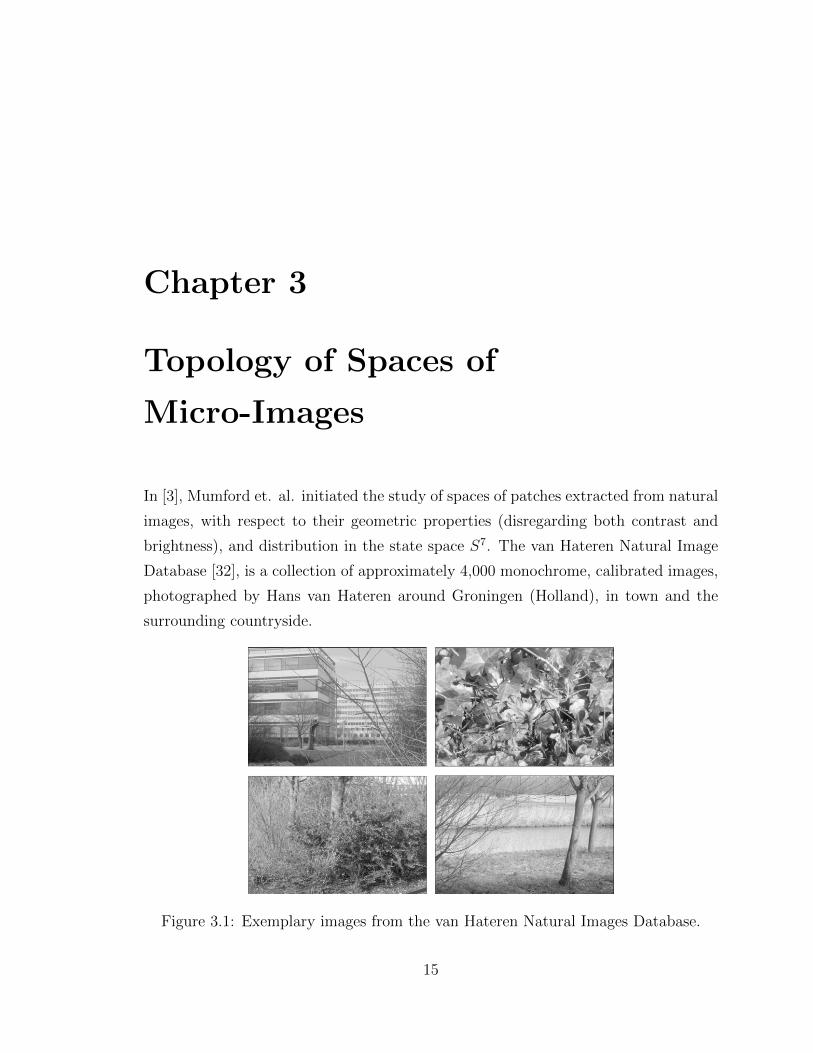
In [3], Mumford et. al. initiated the study of spaces of patches extracted from natural
images, with respect to their geometric properties (disregarding both contrast and
brightness), and distribution in the state space S7. The van Hateren Natural Image
Database [32], is a collection of approximately 4,000 monochrome, calibrated images,
photographed by Hans van Hateren around Groningen (Holland), in town and the
surrounding countryside.
Figure 3.1: Exemplary images from the van Hateren Natural Images Database.
15

CHAPTER 3. TOPOLOGY OF SPACES OF MICRO-IMAGES 16
3.1 The Mumford Formalism
For each image in the database, 5,000 3×3 patches were selected at random, and then
the logarithm of each entry in the patch is calculated. According to Weber’s law, the
ratio ∆L/L between the just noticeable difference ∆L and the ambient luminance L,
is constant for a wide range of values of L. Since it is believed that the human visual
system uses this adaptation, Mumford et. al. attempt to model the set of patches as
close as possible to the way we perceive them.
Next, from the 5, 000 3×3 patches of a single image, the top 20 percent with respect
to contrast is selected. Contrast is measured by means of the D-norm ‖ · ‖D, where
an n × n patch P = [pij] yields the vector v = [v1, . . . , vn2 ]t given by vn(j−1)+i = pij,
and one defines
‖P‖2D =∑r∼t
(vr − vt)2.
Here vr = pij is related (∼) to vt = pkl, if and only if pij is the 4-connected neigh-
borhood of pkl, i.e. if and only if |i − k| + |j − l| ≤ 1. The combinatorial data in
the relation ∼ can be encoded in a symmetric n × n matrix D, and it follows that
‖P‖2D = 〈v,Dv〉. In the case n = 3 the matrix D takes the form:
D =
2 −1 0 −1 0 0 0 0 0
−1 3 −1 0 −1 0 0 0 0
0 −1 2 0 0 −1 0 0 0
−1 0 0 3 −1 0 −1 0 0
0 −1 0 −1 4 −1 0 −1 0
0 0 −1 0 −1 3 0 0 −1
0 0 0 −1 0 0 2 −1 0
0 0 0 0 −1 0 −1 3 −1
0 0 0 0 0 −1 0 −1 2
The vectors from the resulting log-intensity, high-contrast patches are centered
by subtracting their mean, and normalized by dividing by their D-norm. This yields
approximately 4× 10⁶ points in R9, on the surface of a 7-dimensional ellipsoid.
CHAPTER 3. TOPOLOGY OF SPACES OF MICRO-IMAGES 17
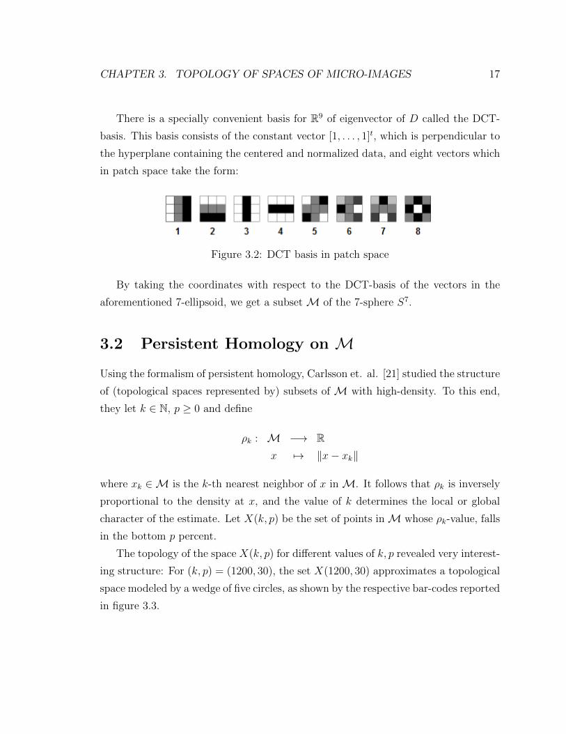
There is a specially convenient basis for R9 of eigenvector of D called the DCT-
basis. This basis consists of the constant vector [1, . . . , 1]t, which is perpendicular to
the hyperplane containing the centered and normalized data, and eight vectors which
in patch space take the form:
Figure 3.2: DCT basis in patch space
By taking the coordinates with respect to the DCT-basis of the vectors in the
aforementioned 7-ellipsoid, we get a subset M of the 7-sphere S7.
3.2 Persistent Homology on M
Using the formalism of persistent homology, Carlsson et. al. [21] studied the structure
of (topological spaces represented by) subsets of M with high-density. To this end,
they let k ∈ N, p ≥ 0 and define
ρk : M −→ Rx 7→ ‖x− xk‖
where xk ∈M is the k-th nearest neighbor of x in M. It follows that ρk is inversely
proportional to the density at x, and the value of k determines the local or global
character of the estimate. Let X(k, p) be the set of points inM whose ρk-value, falls
in the bottom p percent.
The topology of the space X(k, p) for different values of k, p revealed very interest-
ing structure: For (k, p) = (1200, 30), the set X(1200, 30) approximates a topological
space modeled by a wedge of five circles, as shown by the respective bar-codes reported
in figure 3.3.

CHAPTER 3. TOPOLOGY OF SPACES OF MICRO-IMAGES 18
(a) H0-persistence
(b) H1-persistence
(c) H2-persistence
Figure 3.3: Bar-code for X(1200, 30) shows the topology of a wedge of five circles.
With respect to patches, this space can be realized as the three circle model:
(a) (b)
Figure 3.4: (a) A space with the homotopy type of a wedge of 5 circles. The space ismade up of three circles, of which two are disjoint, and the third intercepts each ofthe others at two points. (b) Patches included in the three circle model.
The natural question arising from these findings is whether or not one could
discover in the data, a higher dimensional entity containing the 3-circle model. The
answer was affirmative, and the topological space that emerged was a familiar surface:

CHAPTER 3. TOPOLOGY OF SPACES OF MICRO-IMAGES 19
The set X(100, 10) has topological signatures consistent with either the Klein bottle
or the torus:
(a) H1( · ;Z/2)-persistence
(b) H2( · ;Z/2)-persistence
Figure 3.5: Bar-code for X(100, 10) with Z/2-coefficients reveals a surface.
In order to decide between the Klein bottle and the torus, one only needs to change
the field of coefficients to F3, and repeat the persistent-homology computation. With
this change, the Klein bottle emerged, and a closer study revealed the model:
Figure 3.6: Space of patches corresponding to X(100, 10) parametrizes a Klein bottle.

CHAPTER 3. TOPOLOGY OF SPACES OF MICRO-IMAGES 20
This space can be understood as the set of 3-by-3 patches, whose intensity function
is given by polynomials
p(x, y) = c(ax+ by) + d(ax+ by)2
where a2 + b2 = c2 + d2 = 1. Let this set of polynomials be denoted by K.
The interpretation of the polynomial model is as follows: The angle α ∈ [π/4, 5π/4)
satisfying
eiα = a+ ib
captures the preferred direction of the patch, and it is parametrized by the horizontal
direction on the Klein bottle model. The vertical direction, given by an angle
β ∈ [−π/2, 3π/2) so that
eiβ = c+ id
determines how linear or quadratic the patch will be. Using Monte Carlo simulations,
it was shown that 50% of the points inM accumulate around K, in a tubular neigh-
borhood occupying about 20% of the volume of S7. This should be contrasted with
the fact that M accounts for 84% of the total volume in the 7-sphere.
With this interpretation of the polynomial model K, we will give in the next
chapter a solution to the follow problem: Given a natural image, most of its high-
contrast patches should be in a small tubular neighborhood T of K. How do we
compute the projection map Φ : T −→ K?

Chapter 4
Projecting Samples Onto K
As discussed in the previous chapter, the Klein bottle model captures two patch
features. Namely, the first coordinate measures the preferred direction of the patch,
and once the direction is identified, the second coordinate captures how quadratic
or linear the patch is. Following this insight, we present in this chapter a method
for associating to most high-contrast patches in an image, a point on the idealized
Klein bottle K. Namely, we show that for most high-contrast patches it is possible
to measure its preferred direction as an angle α ∈ [π/4, 5π/4), and given the vector[a
b
]=
[cosα
sinα
]
one can compute the orthogonal projection of the patch (regarded as a function of
two variables x, y) onto the space of polynomial functions
Cα = {c(ax+ by) + d(ax+ by)2 | c2 + d2 = 1}
provided the patch is directional enough.
As a methodological approach, we will first develop the concepts of direction, di-
rectionality and projection onto Cα for patches represented by differentiable functions.
Having this, we will extend the notions to discrete ones. Notice that this method can
be regarded as a continuous version of the Maximum Response 8 (MR8) filter.
21

CHAPTER 4. PROJECTING SAMPLES ONTO K 22
4.1 The Differentiable Case
4.1.1 Direction and Directionality
Let I = [−1, 1]. A square patch from an image in gray scale can be thought of as a
function
f : I2 −→ I
where f(x, y) is the intensity at the pixel (x, y), f(x, y) = −1 if (x, y) is a purely
black pixel and f(x, y) = 1 if (x, y) is a purely white pixel.
Definition 4.1.1. A patch f : I2 −→ I is said to be purely directional, if there exists
a function g : [−√
2,√
2] −→ I and a unitary vector
[a
b
]so that
f(x, y) = g(ax+ by)
for all (x, y) ∈ I2.
Notice that such an f will be constant along lines parallel to
[−ba
].
Theorem 4.1.2. Let f : I2 −→ I be a differentiable patch. Then Qf : R2 −→ Rgiven by
Qf (v) =
∫∫I2
〈∇f, v〉2dxdy
is a positive semi-definite quadratic form so that:
1. If f(x, y) = g(ax+ by), with a2 + b2 = 1 then
Qf (a, b) ≥ Qf (v)
for all ‖v‖ = 1.
2. Letj : S1 −→ RP 1
v 7→ {v,−v}

CHAPTER 4. PROJECTING SAMPLES ONTO K 23
be the projection map and assume the eigenvalues of Af , the matrix representing
Qf , are distinct. Then the direction map
Dir(f) = j(
arg max‖v‖=1
Qf (v))
is a well defined continuous function of f in the C1 topology. Moreover, the
maximum is attained at the eigenvectors of Af with largest eigenvalue.
Proof.
1. If f(x, y) = g(ax+ by), then we have the identity
b∂f
∂x= a
∂f
∂y
and therefore Qf (−b, a) = 0. Notice that by positive semi definiteness of Qf ,
we conclude that Qf attains its global minimum on S1 at
[−ba
]. On the other
hand, by the spectral theorem, there exists an orthogonal matrix B so that if
λ1, λ2 are the eigenvalues of Af , we can write
Af = Bt ·
[λ1 0
0 λ2
]·B.
Since B is orthogonal, ‖v‖ = 1 implies ‖Bv‖ = 1 and if Bv =
[r
s
]we have
Qf (v) = (1− s2)λ1 + s2λ2
It follows that the minimum of Qf on the unit circle is the smallest eigenvalue
of Af , and it is attained at the unitary vectors in its eigenspace.
Likewise, the largest eigenvalue of Af is the maximum of Qf , which is attained
at any unitary vector in its eigenspace. Therefore, if Qf (−b, a) is the minimum,
Qf (a, b) is the maximum and Qf (a, b) ≥ Qf (v) for all ‖v‖ = 1.

CHAPTER 4. PROJECTING SAMPLES ONTO K 24
2. As it was shown (1), max‖v‖=1
Qf (v) is attained at the unitary eigenvectors in the
eigenspace of the largest eigenvalue of Af . Since the eigenvalues of Af are
distinct, their eigenspaces are one dimensional and it follows that the unitary
vectors in each eigenspace are antipodal. Thus Dir is well defined.
Remarks:
1. From here on, we will assume that∫∫‖∇f‖2dxdy = 1 for all differentiable
patches f : I2 −→ I in consideration. This condition is related to normalization
by the D-norm. Indeed, the D-norm is a discrete version of
f 7→
√∫∫‖∇f‖2dxdy
which is the unique scale-invariant norm on images f(x, y).
2. If we let S1 = [0, 2π]/ ∼, where 0 is identified with 2π, then RP 1 can be
identified with [π/4, 5π/4]/ ∼ where π/4 ∼ 5π/4. Via these identifications, we
will regard Dir as a function onto [π/4, 5π/4).
3. The condition of Af not being a scalar matrix cannot be dropped in order to
define the direction of f . Consider the patch f(x, y) =√
323
(x2 + y2). It follows
that ∫∫‖∇f‖2dxdy = 1 and
∫∫〈∇f,
[a
b
]〉2dxdy =
1
2
for all a2 + b2 = 1 and therefore Qf = (1/2)Id. Notice that f is a radial patch,
and therefore its direction is not well defined.
4. For each differentiable patch f , we can define its directionality
dir(f) = |λ1 − λ2|
where λ1, λ2 are the eigenvalues of Af .

CHAPTER 4. PROJECTING SAMPLES ONTO K 25
It follows that dir(f) is maximized when f is a purely directional patch, for
radial patches dir(f) = 0, and therefore dir(·) measures how directional a patch
is.
A discrete version of dir(f) was used in [20] as a thresholding function, (along
with two other quantities measuring characteristics of a patch) in order to re-
cover the high density regions in M.
5. The same results described above remain true for differentiable functions
f : I2 −→ [u, v]
where −∞ < u < v <∞. In particular, when f is a log-intensity patch.
4.1.2 Projection onto CαLet α ∈ [π/4, 5π/4), eiα = a+ ib, u = ax+ by and v = −bx+ ay for (x, y) ∈ I2. Let
U = Uα = {(ax+ by,−bx+ ay) | (x, y) ∈ I2}
and let L2(U) be the space of real valued square-integrable functions on U , equipped
with the inner product
〈f, g〉 =
∫U
f(u, v)g(u, v)dµ.
From the Stone-Weierstrass theorem and the fact that continuous functions are dense
in L2, we conclude that the set of polynomials in the variables u, v is dense in L2(U).
Let f ∈ L2(U) be so that 〈f, unvm〉 = 0 for all n,m ∈ N∪{0} and let us assume that
‖f‖ > 0. Thus, there exists a polynomial p(u, v) so that ‖f − p‖ < ‖f‖2
and from the
orthogonality relations 〈f, unvm〉 = 0 we get
‖f‖2 = ‖f − p‖2 − ‖p‖2
<‖f‖2
4− ‖p‖2

CHAPTER 4. PROJECTING SAMPLES ONTO K 26
which is a contradiction. This shows that by applying Gram-Schmidt to the set of
monomials {unvm | n,m ≥ 0} with indexing (n,m) 7→ (n+m)(n+m+ 1)/2 + n, we
obtain a complete orthonormal subset S of L2(U).
It follows that any f ∈ L2(U) can be polynomially represented as
∑s∈S
〈f, s〉s.
Now, for each function f : I2 −→ I one can define fα(u, v) = f(au− bv, bu+ av)
and when f is a differentiable patch, which is also purely directional with direction
α, we have∂fα∂v
= 0.
From this perspective, α = Dir(f) can be interpreted as the angle that in average,
makes fα as independent from v as possible. It follows that one can represent fα in
terms of polynomials s ∈ S depending only on u, and if one further requires the patch
to be centered, that is∫Ufαdµ = 0, then the degree two polynomial approximation
becomes
fα ≈ 〈fα, u〉u
‖u‖2+ 〈fα, u2〉
u2
‖u2‖2
= rα(c(ax+ by) + d(ax+ by)2
)for some rα ≥ 0 and c2 + d2 = 1. This follows by tracing back the Gram-Schmidt
orthonormalization on the set {1, v, u, v2, uv, u2} and checking that u and u2 are
perpendicular.
Definition 4.1.3. Let f : I2 −→ I be a differentiable patch so that dir(f) > 0.
If Dir(f) = α, fα ≈ rα(c(ax + by) + d(ax + by)2
)is its degree two polynomial
approximation and rα > 0, then
Φ(f) = c(ax+ by) + d(ax+ by)2
is the projection of f onto Cα.

CHAPTER 4. PROJECTING SAMPLES ONTO K 27
Remark: Even when Cα is not a linear subspace of L2(U), we use the term “projection”
in the sense that c(ax+ by) + d(ax+ by)2 attempts to minimize the L2-distance from
fα to Cα. Since in the case of linear subspaces of L2(U) the concepts of orthogo-
nal projection and distance minimizer coincide, then the abuse of language is mildly
justified.
Now, since K =⋃α
Cα then by composing with the inclusion Cα ⊆ K, we get the
projection of f onto the idealized Klein bottle K.
We will now describe a model for K which is more amenable for computations.
Let S1 ⊆ C be the unit circle inside the complex plane, and let T = S1 × S1 be the
torus. Notice that T is equipped with a free Z/2Z action, defied by
1 · (z, w) = (−z, w)
with orbit space homeomorphic to K = [π/4, 5π/4] × [−π/2, 3π/2]/ ∼, where ∼stands for the identification of (x,−π/2) with (x, 3π/2) and that of (π/4, π+ y) with
(5π/4, π − y), |y| ≤ π. It follows that K is the usual model for the Klein bottle and
we have a quotient map
q : S1 × S1 −→ K.
It is this quotient map and the induced homomorphism q∗ : L2(K) −→ L2(S1×S1)
which will allow us to do Fourier analysis on the Klein bottle.
Definition 4.1.4. Let Φ(f) = c(ax+ by) + d(ax+ by)2 and let (α, β) ∈ K be so that
eiα = a+ ib and eiβ = c+ id. We let
Ψ(f) = (α, β) ∈ K
be the projection of f onto K.

CHAPTER 4. PROJECTING SAMPLES ONTO K 28
4.2 The Discrete Case
4.2.1 Direction and Directionality
Let P be a 3× 3 patch represented by the 3× 3 matrix P = [pij], and let us identify
it with the function that takes the value pij on the region
Rij = {(x, y) ∈ I2 : |x− rj|+ |y − ri| < 1/3} rj = 2(j − 2)/3, ri = 2(2− i)/3.
A delicate step toward extending the definition of the direction of a differentiable
patch to a discrete one, is the choice of discretization for the gradient. For the
integral we use ∫∫F (x, y)dxdy ≈
∑ij
F (rj, ri).
Let us show with an example why this is a subtle issue. If we discretize the partial
derivatives of P using the formulae:
Px(x, y) =
pi2 − pi1 if (x, y) ∈ Ri1
pi3−pi12
if (x, y) ∈ Ri2
pi3 − pi2 if (x, y) ∈ Ri3
(the ones for Py being similar) then for the patch
which can be represented (up to a positive multiple) by the matrix
F =
1 1 0
1 0 1
0 1 1

CHAPTER 4. PROJECTING SAMPLES ONTO K 29
we get that
AF (x, y) =
[9/2 0
0 9/2
]and therefore, every vector in the unit circle corresponds to a unitary vector in the
eigenspace of the largest eigenvalue of AF . One would like, however, this patch to
have direction e3πi/4. If instead, using the first order approximation
∇f(dx) ≈ ∇f(0) +Hess f(0)dx
we let
∇P (x, y) = ∇P (0, 0) +HessP (0, 0) ·
[j − 2
2− i
], (x, y) ∈ Rij
where
∇P (0, 0) =1
2
[p23 − p21p12 − p32
]
HessP (0, 0) =1
2
[p23 − 2p22 + p21
p13−p11−p33+p312
p13−p11−p33+p312
p12 − 2p22 + p32
]
then applying this definition to our example we get
QF (x, y) =[x y
]·
[5/2 −2
−2 5/2
]·
[x
y
].
Notice that the unitary vector corresponding to the largest eigenvalue is now e3πi/4.
The conclusion from this example is that when trying to approximate the gradient
at a point, one should use as many neighboring pixels as possible. This, to ensure
that the global direction is measured correctly. We will study in the next paragraphs
how to carry out this computations for patches of size k×k, for some choices of k > 3.

CHAPTER 4. PROJECTING SAMPLES ONTO K 30
An important feature of natural images is their multi-scale hierarchical organiza-
tion. In textures for example, one encounters that observations at various distances
may reveal different patterns. It is for this reason that robust invariants should in-
clude multi-scale information, and ways of tracking the scale evolution of features.
The distribution on the Klein bottle of high-contrast patches coming from an
image, can be turned into a multi-scale invariant by analyzing the evolution of the
distribution as the number of pixels increases. We have chosen here to study patches
of size (3(2n−1))× (3(2n−1)) for n = 1, 2, 3, 4, 5. The reasons behind this choice are
the following: When trying to describe a discretization for the gradient, there are two
things to keep in mind. On the one hand, when approximating the partial derivatives
at a point one should use as much information as possible from neighboring pixels, so
that the global direction is measured accurately. On the other hand, the derivative
is only a local concept and therefore its computation should not involve interactions
between distant pixels. Thus, we choose sizes that allows us to make the computations
locally and the localization coherent as we move throughout the patch.
Given a patch P of size (3(2n− 1))× (3(2n− 1)), this can be divided into disjoint
3 × 3 sub-patches, whose centers we label. For any pixel p in P , there exists a
unique labeled center c closest to it, and using this center we compute the first order
approximation
∇P (p) = ∇P (c) +HessP (c) · u
where u ∈ {−1, 0, 1} × {−1, 0, 1} is the position of p with respect to c.
If by way of example we represent the 3× 3 sub-patch with center c containing p
(in position (1, 1)) as
c−1,1 c0,1 p
c−1,0 c c1,0
c−1,−1 c0,−1 c1,−1

CHAPTER 4. PROJECTING SAMPLES ONTO K 31
then u =
[1
1
]and ∇P (c) = 1
2
c1,0 − c−1,0
c0,1 − c0,−1
.
An expression for HessP (c) is a little more involved. In general, a patch P of
size (3(2n− 1))× (3(2n− 1)) has three types of 3× 3 sub-patches, according to their
location with respect to the boundary of P :
I II II II I
II III III III II
II III III III II
II III III III II
I II II II I
so we compute the Hessian for the center of each type as follows:
• For sub-patches of type I, 4HessP (c) is given according to its location by
[c2,0 − 3c+ 2c−1,0 c1,1 − c1,−1 − c−1,1 + c−1,−1
c1,1 − c1,−1 − c−1,1 + c−1,−1 c0,−2 − 3c+ 2c0,1
]top left
[c2,0 − 3c+ 2c−1,0 c1,1 − c1,−1 − c−1,1 + c−1,−1
c1,1 − c1,−1 − c−1,1 + c−1,−1 c0,2 − 3c+ 2c0,−1
]bottom left

CHAPTER 4. PROJECTING SAMPLES ONTO K 32
[2c1,0 − 3c+ c−2,0 c1,1 − c1,−1 − c−1,1 + c−1,−1
c1,1 − c1,−1 − c−1,1 + c−1,−1 c0,−2 − 3c+ 2c0,1
]top right
[2c1,0 − 3c+ c−2,0 c1,1 − c1,−1 − c−1,1 + c−1,−1
c1,1 − c1,−1 − c−1,1 + c−1,−1 c0,2 − 3c+ 2c0,−1
]bottom right
• For sub-patches of type II, 4HessP (c) is given according to its location by
[c2,0 − 2c+ c−2,0 c1,1 − c1,−1 − c−1,1 + c−1,−1
c1,1 − c1,−1 − c−1,1 + c−1,−1 c0,−2 − 3c+ 2c0,1
]top
[c2,0 − 2c+ c−2,0 c1,1 − c1,−1 − c−1,1 + c−1,−1
c1,1 − c1,−1 − c−1,1 + c−1,−1 c0,2 − 3c+ 2c0,−1
]bottom
[c2,0 − 3c+ 2c−1,0 c1,1 − c1,−1 − c−1,1 + c−1,−1
c1,1 − c1,−1 − c−1,1 + c−1,−1 c0,2 − 2c+ c0,−2
]left
[c−2,0 − 3c+ 2c1,0 c1,1 − c1,−1 − c−1,1 + c−1,−1
c1,1 − c1,−1 − c−1,1 + c−1,−1 c0,2 − 2c+ c0,−2
]right
• For sub-patches of type III
HessP (c) =1
4
[c2,0 − 2c+ c−2,0 c1,1 − c1,−1 − c−1,1 + c−1,−1
c1,1 − c1,−1 − c−1,1 + c−1,−1 c0,2 − 2c+ c0,−2
].
Equipped with the discretization for the gradient, we can know compute AP ,
dir(P ), Dir(P ) whenever dir(P ) ≥ tk and Ψ(P ) whenever rad(P ) > 0. Here tk
(k = 1, . . . , 5) is a threshold to be determined.

CHAPTER 4. PROJECTING SAMPLES ONTO K 33
Let I be a digital image in gray scale. We describe now the process for constructing
families of samples on the Klein bottle, from the sets of high-contrast log-intensity
k × k patches of I.
Constructing the Family of Samples
1. For each k = 3(2n− 1) (n = 1, . . . , 5), let Pk be the set of k× k patches from I.
2. According to its bit depth, a patch P ∈ Pk is an integer matrix of size k × k,
with entries between 0 and 2d−1. Here d is the bit depth, which is usually equal
to 8 or 16. Let P be the patch obtained from P by adding 1 to each entry and
computing its logarithm. Let P be the patch obtained from P by subtracting
its mean from each entry and denote the resulting set by Pk.
3. For each k and each P ∈ Pk, compute its D-norm
‖P‖D =
√∑i∼j
(pi − pj)2
where P = [prs], pk(s−1)+r = prs and i ∼ j if and only if pi is in the 4-connected
neighborhood of pj. Keep the patch P if its D-norm falls within the top 30%
with respect to Pk.
4. For each k = 3(2n− 1) (n = 1, . . . , 5) let
Sn(I) = {Ψ(P ) | P ∈ Pk, dir(P ) ≥ tk and rad(P ) > 0}.
It follows that Sn(I) ⊆ K is a sample on the Klein bottle.
We have now, modulo estimating the tk’s, a complete method for associating to
each digital image I in gray scale, a sequence Si(I) of samples on the Klein bottle K.
We will study the estimation problem in what remains of this section.

CHAPTER 4. PROJECTING SAMPLES ONTO K 34
4.2.2 Estimating tk
As discussed earlier, dis(·) is a measure of how directional a patch is and Dir(P )
computes this preferred direction whenever dir(P ) > 0. Nevertheless, it is expected
that the determined and perceived directions disagree for small values of dir, and
therefore the role of tk will be to assure their agreement, whenever dir ≥ tk. In other
words, evaluating the condition dir(P ) ≥ tk amounts to deciding wether P is close
enough to K so that applying the projection Φ : T −→ K makes sense.
The estimation of the thresholds tk was carried out using the USC-SIPI Texture
database. We describe now this set of image textures. The USC-SIPI Image Database
is a collection of digitized images, maintained by the Signal and Image Processing
Institute (SIPI) at the University of Southern California [46]. The Textures volume
contains 154 images, all monochrome of sizes 512× 512 and 1024× 1024. Most of the
images in this set are digitized versions of pictures in the Brodatz book [41].
(a) Bark (b) Straw (c) Wood Grain
Figure 4.1: Exemplary images from the Broadtz collection, digitized in the USC-SIPITexture database.
Using the USC database, we now study how the perceived direction is related to
Dir(P ), as dir(P ) increases. To this end, we construct the sets Pk (refer to step
2 in Constructing the Family of Samples) for all images in the USC database
and record for each patch its direction in directionally. The results for k = 3, 9 are
summarized in figure 4.2.

CHAPTER 4. PROJECTING SAMPLES ONTO K 35
(a) Evolution of 3× 3 patches.
(b) Evolution of 9× 9 patches.
Figure 4.2: Perceived directionality and Dir as a functions of dir. dir increases tothe right and down. Dir is measured in degrees.

CHAPTER 4. PROJECTING SAMPLES ONTO K 36
The threshold tk is then determined (using the full set of k × k patches from the
USC Database) as the value of dir, in which the perceived and computed directions
begin to agree in a consistent fashion. In table 4.1 we summarize the estimated
thresholds.
Table 4.1: Estimated thresholdsk 3 9 15 21 27tk 0.030 0.013 0.045 0.043 0.070
To have an idea of the percentage of patches we discard when thresholding by tk,
we present in figure 4.3 the histograms of directionalities for k = 3, 9.
(a) Directionality 3× 3 patches
(b) Directionality 9× 9 patches
Figure 4.3: Histogram of directionalities, USC Texture Database

CHAPTER 4. PROJECTING SAMPLES ONTO K 37
In summary, we have developed a method for associating to each image I, a
sequence of samples Si(I) on the Klein bottle K with underlying probability density
functions
hi(I) : K −→ R.
One of our final goals is to study what attributes of I are captured by the sequence
{hi(I)}, and compare these sequences for different images I. In order to do so, it is
necessary to device compact, discrete and faithful representations of estimators for
hi, as well as ways of comparing these representations. This problem will be the main
focuss of the next chapter, where ideas from Fourier analysis and density estimation
will be combined.

Chapter 5
A Discrete Representation
Density estimation from finite samples lies at the center of statistics as one of the
most fundamental questions. In fact, many applications of statistical methods reduce
to the estimation of some parameters, or the full probability density function (PDF)
underlying the phenomenon. It is for this reason that several methods, following vari-
ous heuristics, have been devised to solve different instances of the density estimation
problem. See for example [8] for a nice survey.
One idea that stands out from this constellation of strategies, is that estimating
a PDF can be translated into estimating an at most countable set of scalars, which
is extremely appealing for finite representation purposes. If the PDF is, for instance,
assumed to be in a particular parametric family, then one estimates the set of pa-
rameters. In this direction, the most general approach is perhaps the one given by
orthogonal series estimators. Let H be a separable Hilbert space and let {φk}k∈Z be
an orthonormal basis for H. Under the assumption that f ∈ H, one can write
f =∑k
fkφk
where convergence of the series is in the topology of H, and the estimation of f can
be translated into the estimation of the fk’s. Notice that a finite number of the fk’s
might be enough for representation purposes, depending on the rate of convergence
of the series.
38
CHAPTER 5. A DISCRETE REPRESENTATION 39
A popular choice for H is the space of square-integrable functions on the unit
circle, where one can take φk(x) = eikx. In what follows we will take H = L2(M),
where (M,A , µ) is a measure space, A countably generated and µ σ-finite, to assure
the separability of L2(M).
Natural questions arise in this setting:
• Are there “good” estimators fk for fk?
• How good is the statistic
f =∑k
fkφk.
• How does the accuracy depend on the sample size?
Fortunately, the literature in statistics gives encouraging answers to these ques-
tions, with inspiration coming from the case M = Rn.
5.1 Coefficient Estimation in L2
Let S (Rn) be the space of rapidly decreasing complex valued functions on Rn (see
[36]). It follows that for each c ∈ Rn, the Dirac delta function centered at c
δ(x− c) : S (Rn) −→ Cϕ 7→ ϕ(c)
is a continuous linear functional and therefore a tempered distribution. That is, an
element in the dual space S ′(Rn) = S (Rn)∗. An application of integration by parts
shows that:
Proposition 5.1.1. For every ϕ ∈ S (Rn) one has that
limk→∞
∫Rn
ϕ(x)k√πne−k
2‖x−c‖2dµ(x) = ϕ(c).
Thus δ(x − c) is a weak limit of Gaussians with mean c, as the variance approaches
zero.

CHAPTER 5. A DISCRETE REPRESENTATION 40
What this result tells us, is that δ(x − c) can be interpreted as the generalized
function bounding unit volume, that is zero at x 6= c and an infinite spike at c.
Moreover, if X1, . . . , XN are i.i.d. random variables with probability density function
f : Rn −→ R
where f ∈ L2(Rn), then as a “generalized statistic”
fδ(X) =1
N
N∑i=1
δ(X −Xi)
can be thought of as the Gaussian Kernel estimator (see [8]) with infinitely small
width.
Let {φk} be an orthonormal basis for L2(Rn). What we will see shortly, is that
an appropriate definition of the coefficients of fδ with respect to {φk}, yields good
estimators for those of f . To motivate the definition, let us consider the following
example: Let φα : Rn −→ R be given by
φα(x1, . . . , xn) = hα1(x1) · · ·hαn(xn)
where α = (α1, . . . , αn) ∈ Nn and hk is the k-th Hermite function (or harmonic
oscillator wave function) on R. It follows that {φα} is an orthonormal basis for
L2(Rn) (Lemma 3, page 142, [36]) and from the N -representation theorem (V.14 ,
[36]) we get that ∑α
T (φα)φα
converges to T in the weak-∗ topology, for all T ∈ S ′(Rn). Here we are using
S (Rn) ⊆ L2(Rn) ⊆ S ′(Rn), and T (φα) = T (φα).
From this example, it is natural to make the following definition.
Definition 5.1.2. Let {φk} be an orthonormal basis for L2(Rn), and let T ∈ S ′(Rn).
We define Tk = T (φk) as the coefficients of T with respect to {φk}.
CHAPTER 5. A DISCRETE REPRESENTATION 41
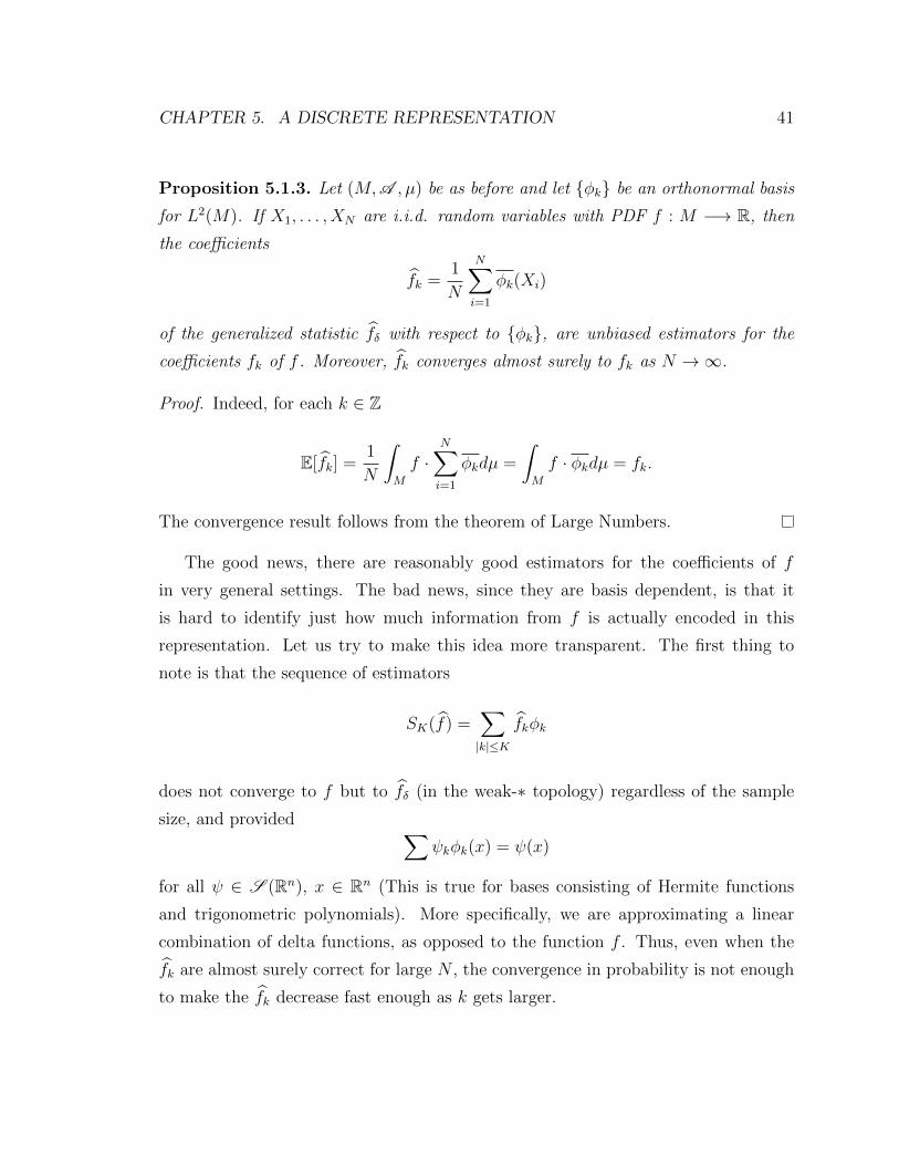
Proposition 5.1.3. Let (M,A , µ) be as before and let {φk} be an orthonormal basis
for L2(M). If X1, . . . , XN are i.i.d. random variables with PDF f : M −→ R, then
the coefficients
fk =1
N
N∑i=1
φk(Xi)
of the generalized statistic fδ with respect to {φk}, are unbiased estimators for the
coefficients fk of f . Moreover, fk converges almost surely to fk as N →∞.
Proof. Indeed, for each k ∈ Z
E[fk] =1
N
∫M
f ·N∑i=1
φkdµ =
∫M
f · φkdµ = fk.
The convergence result follows from the theorem of Large Numbers.
The good news, there are reasonably good estimators for the coefficients of f
in very general settings. The bad news, since they are basis dependent, is that it
is hard to identify just how much information from f is actually encoded in this
representation. Let us try to make this idea more transparent. The first thing to
note is that the sequence of estimators
SK(f) =∑|k|≤K
fkφk
does not converge to f but to fδ (in the weak-∗ topology) regardless of the sample
size, and provided ∑ψkφk(x) = ψ(x)
for all ψ ∈ S (Rn), x ∈ Rn (This is true for bases consisting of Hermite functions
and trigonometric polynomials). More specifically, we are approximating a linear
combination of delta functions, as opposed to the function f . Thus, even when the
fk are almost surely correct for large N , the convergence in probability is not enough
to make the fk decrease fast enough as k gets larger.

CHAPTER 5. A DISCRETE REPRESENTATION 42
The conclusion: taking more coefficients is not necessarily a good thing, so instead
we could try to make an educated guess about {φk} that improves our chances in terms
of representation accuracy.
Some observations about the type of probability density functions modeling the
distribution of small patches coming from natural scenes, are pertinent:
1. Natural images often come as compositions of various scenes. That is, small
patches coming from different locations in the image are likely to have different
directions and different gradients. Also, since the camera averages intensities
locally, most transitions from linear to quadratic gradients in the same direction,
vary continuously. This implies that any random sample of high density patches
tends to cover large connected portions of the Klein bottle, and therefore the
associated PDF is not likely to be localized in space. This observation suggests
that the basis {φk} should be of global character, eliminating candidates such
as the ones coming from wavelets.
2. An aspect inherent to the geometric model, is that elements in L2(K) will have
as domain a quotient of S1×S1. Thus by pre-composing with the quotient map,
they can be regarded as 2π-periodic functions. Appropriate linear combinations
of the set of functions
φnm(x, y) = einx+imy
emerges then as a natural candidate.
Since the higher degree Fourier coefficients tune the fine scale details of the ap-
proximation, it follows that most of the information about the PDF is encoded in the
low frequencies. That is, truncating the series is sensible in a heuristic sense.
It is known ([22]) that truncation is also nearly optimal with respect to mean
integrated square error (MISE), within a natural class of statistics for f . Indeed, if
within the family of estimators
f ∗N =∞∑k=1
λk(N)fkφk

CHAPTER 5. A DISCRETE REPRESENTATION 43
one looks for the sequence {λk(N)}k∈N that minimizes
MISE = E[‖f ∗N − f‖22]
then provided the fk (k ≤ K(N)) are large compared with n−1var(φk) and the fk
(k > K(N)) are negligible, then λk(N) = 1 for k ≤ K(N) and zero otherwise,
has a nearly optimal mean square error. Notice that this is the expected behavior
for trigonometric bases. Refer to [37] for another inclusion criterion using only the
derived estimates fk, and the sample size N .
In summary, not only is it possible to encode the information from f in a finite
set of easily computable estimators, but this truncation is nearly optimal in a precise
sense. We will proceed now to find a version of the Fourier basis for the case in which
M is the Klein bottle.
5.2 An Orthonormal Basis for L2(K)
Let S1 be the unit circle, and let M(S1,C) be the set of complex valued (Lebesgue)
measurable functions on S1. We identify M(S1,C) with the set of functions
f : R −→ C
which are measurable and so that f(x+ 2π) = f(x) for all x ∈ R. If f, g ∈M(S1,C),
we define
〈f, g〉S1 =1
2π
∫S1
fgdτ
where τ is the Lebesgue measure on [0, 2π]. Let L2(S1) be the set of equivalence
classes [f ] (with respect to equality almost everywhere) of functions f ∈M(S1,C) so
that 〈f, f〉S1 <∞. By abuse of notation we will write f instead of [f ].

CHAPTER 5. A DISCRETE REPRESENTATION 44
Theorem 5.2.1. 〈·, ·〉S1 defines an inner product on L2(S1) so that (L2(S1), 〈·, ·〉S1) is
a Hilbert space. Moreover, the set of functions B = {einτ | n ∈ Z} is an orthonormal
basis for L2(S1). That is, if f(n) = 〈f, einτ 〉S1 then
SN(f)(τ) =N∑
n=−N
f(n)einτ
converges to f in the L2-norm
‖f‖2S1 = 〈f, f〉S1 .
We will show now that a similar result holds for the Klein bottle. Let K be as in
definition 4.1.4, and let
M(K,C) = {f : S1 × S1 −→ C | f is measurable and f(x+ π,−y) = f(x, y)}
be the set of complex valued measurable functions on K. Let
〈f, g〉K =1
(2π)2
∫K
fgdκ
for f, g ∈M(K,C), κ being the Lebesgue measure on [0, π]× [0, 2π], and define
L2(K) = {[f ] | f ∈M(K,C) and 〈f, f〉K <∞}.
Theorem 5.2.2. Let n ∈ Z, m ∈ N ∪ {0} and let
φn,m(x, y) = einx+imy + (−1)neinx−imy.
Then (L2(K), 〈·, ·〉K) is a Hilbert space and B = {φn,m | m = 0 implies n = 2k} is an
orthogonal basis for L2(K) with respect to 〈·, ·〉K. That is, if
‖f‖2K = 〈f, f〉K

CHAPTER 5. A DISCRETE REPRESENTATION 45
is the induced L2-norm and f(n, ,m)·‖φn,m‖2K = 〈f, φn,m〉K, then for every f ∈ L2(K)
limN→∞
∥∥∥ N∑m=0
N∑n=−N
f(n,m)φn,m − f∥∥∥K
= 0.
Proof. We defer the proof of this result to appendix A.
In the case of real valued functions we have the following
Corollary 5.2.3. Let f : K −→ R be a square integrable function. Then
N∑m=0
N∑n=−N
f(n,m)φnm =1
2π2+
N∑m=1
am(2 cosmy) +
N0∑n=1
bn(2 cos 2nx) + cn(2 sin 2nx)
+N∑
n,m=1
dnm
(2√
2 cos(nx) · sin(my +
π
4(1 + (−1)n)
))+
N∑n,m=1
enm
(2√
2 sin(nx) · sin(my +
π
4(1 + (−1)n)
))
converges to f with respect to the norm ‖ · ‖K as N → ∞. Here N0 = bN2c. The
functions between parentheses on the right hand side of the equality are orthonormal
with respect to 〈· , ·〉K, and thus the coefficients am, bn, cn, ddm, enm can be computed
through inner products with f . That is,
am = 〈f, 2 cos(my)〉K , bn = 〈f, 2 cos(2nx)〉K , etc.
We will refer to this set of functions as the trigonometric basis on the Klein bottle.
5.3 The v-Invariant
Let I be an image in gray scale and for each k = 3(2i − 1), let Si(I) ⊆ K be
the projection onto the Klein bottle of (a sample of) the high-contrast log-intensity
k × k patches from I. If hi(I) : K −→ R is the underlying PDF, then under the
assumption of square-integrability, it can be written as an infinite series in terms of

CHAPTER 5. A DISCRETE REPRESENTATION 46
the trigonometric basis on the Klein bottle as
hi(I) =1
2π2+∞∑m=1
am(2 cosmy) +∞∑n=1
bn(2 cos 2nx) + cn(2 sin 2nx)
+∞∑
n,m=1
dnm
(2√
2 cos(nx) · sin(my +
π
4(1 + (−1)n)
))+
∞∑n,m=1
enm
(2√
2 sin(nx) · sin(my +
π
4(1 + (−1)n)
)).
If we write Si(I) = {P 1k , . . . , P
Nk } where P r
k = (Xrk , Y
rk ), then for each n,m ∈ N
we have the unbiased estimates (by proposition 5.1.3 and corollary 5.2.3)
am =1
2Nπ2
N∑r=1
cos(mY rk )
bn =1
2Nπ2
N0∑r=1
cos(2nXrk)
cn =1
2Nπ2
N0∑r=1
sin(2nXrk)
dnm =1√
2Nπ2
N∑r=1
cos(nXrk) · sin
(mY r
k +π
4(1 + (−1)n)
)enm =
1√2Nπ2
N∑r=1
sin(nXrk) · sin
(mY r
k +π
4(1 + (−1)n)
)for the coefficients of hi(I) with respect to the trigonometric basis on the Klein bottle.
From the frequencies of the various sines and cosines involved, we can assign to
each estimated coefficient a degree
deg(am) = m
deg(bn) = deg(cn) = 2n
deg(dnm) = deg(enm) = n+m

CHAPTER 5. A DISCRETE REPRESENTATION 47
and endow the multi-set
Ci(I) = {am, bn, cn, dnm, enm | n,m ∈ N}
with a partial order � as follows: Let u, v ∈ Ci(I) be distinct (not necessarily as
values, but as elements of the multi-set),
1. If deg(u) < deg(v) then u ≺ v.
2. If deg(u) = deg(v) and u is less than v with respect to the grammatical order
then u ≺ v. The grammatical order on Ci(I) is given by the letters without
their sub-indices (e.g. am ≺ bn, for all m,n).
3. If deg(u) = deg(v) and u ≈ v with respect to the grammatical order, (e.g.
d12 and d21) then u ≺ v if u is less than v with respect to the natural order
(n,m) 7→ (n+m− 2)(n+m− 1)/2 + n.
Definition 5.3.1. Let I be an image in gray scale and let i ∈ N. Given a maximum
degree D ∈ N, the v-Invariant at scale k = 3(2i− 1) bounded by D is the vector
vi(I) = (vi1, . . . , vid)
where {vi1, . . . , vid} = {v ∈ Ci(I) | deg(v) ≤ D} and the indexing is induced by �.
We define the (multi-scale) v-Invariant v(I) as the matrix whose i-th row is vi(I).
The v-Invariant is the construction we propose in this thesis, as a way of capturing
the distribution of high-contrast small patches from an image. In what follows we
will study visualization methods, dissimilarity measures for discrimination purposes,
and its behavior under image rotation.

CHAPTER 5. A DISCRETE REPRESENTATION 48
In order to visualize the information contained in vi(I), we will use the heat-map
associated to the estimated probability density function
hi(I)(x, y) =1
2π2+
D∑m=1
am(2 cosmy) +
D0∑n=1
bn(2 cos 2nx) + cn(2 sin 2nx)
+D∑
n+m=1
dnm
(2√
2 cos(nx) · sin(my +
π
4(1 + (−1)n)
))+
D∑n+m=1
enm
(2√
2 sin(nx) · sin(my +
π
4(1 + (−1)n)
)).
whereD0 = bD2c. That is, the color distribution on the fundamental domain [π/4, 5π/4]×
[−π/2, 3π/2], where the color value at (x, y) is given by hi(I)(x, y).
CHAPTER 5. A DISCRETE REPRESENTATION 49
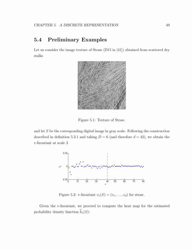
5.4 Preliminary Examples
Let us consider the image texture of Straw (D15 in [41]) obtained from scattered dry
stalks
Figure 5.1: Texture of Straw.
and let S be the corresponding digital image in gray scale. Following the construction
described in definition 5.3.1 and taking D = 6 (and therefore d = 42), we obtain the
v-Invariant at scale 3
Figure 5.2: v-Invariant v1(S) = (v1, . . . , vd) for straw.
Given the v-Invariant, we proceed to compute the heat map for the estimated
probability density function h1(S):

CHAPTER 5. A DISCRETE REPRESENTATION 50
(a) S1(S) (b) Heat-Map h1(S)
Figure 5.3: (a) Projected Sample of 3 × 3 patches from Straw. (b) Estimated heatmap for D = 6, d = 42.
The representation power of the v-Invariant is evident. With a total degree as small
as 6, one already has a heat-map that accurately describes the distribution of S1(S).
It is worth comparing the heat-map with the Klein bottle model
In order to understand what patches appear in S1(S), and their distribution on K.

CHAPTER 5. A DISCRETE REPRESENTATION 51
From this comparison we can draw the following conclusions:
1. The hotter spots on the heat-map (modes of h1(S)) correspond roughly to linear
patches with direction 3π4
. Thus, the horizontal position of hot spots in the heat
map encode observable direction of the image texture. On the other hand, the
vertical position determines the size of the features in the image. That is,
features coming from quadratic patches are regarded as smaller than the ones
coming from linear ones.
2. The extent to which the heat map is confined to a vertical strip and the width
of the band, reflect the directionality of the texture at the given scale. Indeed,
if the image is purely directional, then so are its high-contrast patches, they will
all have roughly the same direction and therefore the heat-map of the estimated
PDF will be confined to a narrow vertical strip. The converse is not true in
general; that is, there are textures with heat maps (at some scales) confined
to a narrow vertical strip even when the images are not directional. The idea
is that small purely directional patches, all with the same direction, can be
arranged in patterns distorting the perceived global directionality. One expects
nevertheless, that if the vertical strip condition holds across all scales, then the
image will be purely directional.
3. There is a dominance in linear patches with an specific gradient orientation.
The orientation of the gradient is dominant in the southeast direction and comes
from the intensity of the heat at y = π2. By zooming into the image, we see
that this observation is consistent with the shadowing of the stalks and their
location against the black background. It follows that the v-Invariant is sensitive
to changes in light source.
4. The diffusion in the heat-map contains information regarding the roughness of
the material. Indeed, diffusion in the heat can be interpreted as local small
variations of direction and feature size of the high-contrast patches. This is
exactly the effect created by irregular shadowing throughout the texture, which
in turn is caused by lack of smoothness in the material.

CHAPTER 5. A DISCRETE REPRESENTATION 52
5. The vertical alignment of the modes of h1(S) is also a measure of the dominant
direction in the texture. In rough materials, where the diffusion on the heat-
map tends to be large, the vertical strip condition may not hold. Nevertheless,
the vertical alignment of hot spots is an evidence of a dominant direction in the
image.
6. The transition in gradient orientation between linear patches, is only through
quadratic patches depicting bright configurations. Since this is certainly not an
artifact of the representation, it would be interesting to understand what this
observation translates into, when one looks at the actual image.
7. Another observation that requires a deeper understanding, is the strong mirror
symmetry with respect to x = 3π4
and y = π2.
A crucial aspect about these observation is that they indeed refer to properties
of image textures captured by the heat-map, as opposed to mere artifacts of the
construction. In what follows we provide examples of how all these properties vary
as a function of the input texture. Let us take ensemble 1 to be the collection:
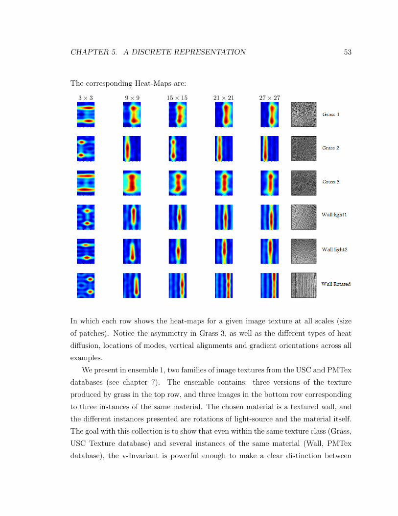
CHAPTER 5. A DISCRETE REPRESENTATION 53
The corresponding Heat-Maps are:
3× 3 9× 9 15× 15 21× 21 27× 27
In which each row shows the heat-maps for a given image texture at all scales (size
of patches). Notice the asymmetry in Grass 3, as well as the different types of heat
diffusion, locations of modes, vertical alignments and gradient orientations across all
examples.
We present in ensemble 1, two families of image textures from the USC and PMTex
databases (see chapter 7). The ensemble contains: three versions of the texture
produced by grass in the top row, and three images in the bottom row corresponding
to three instances of the same material. The chosen material is a textured wall, and
the different instances presented are rotations of light-source and the material itself.
The goal with this collection is to show that even within the same texture class (Grass,
USC Texture database) and several instances of the same material (Wall, PMTex
database), the v-Invariant is powerful enough to make a clear distinction between

CHAPTER 5. A DISCRETE REPRESENTATION 54
them. One of the main objectives, certainly, is to quantify how this distinctions are
made. We discuss some ideas in this regard on chapter 6.
We now turn our attention to ensemble 2 :
in which we present a wide range of textures; going from naturally occurring (Grass)
to man-made materials (Fabric), regular (Fabric 3) to irregular patterns (Fabric 4),
with a multi-scale hierarchy (Fabric 3) and all levels of competing directions (Plastic
bubbles, Pebbles, Metal Plates). The main goal with this ensemble, is to use the
diversity in the collection to show how the observations about the heat map for
h1(S), vary in terms of the input image.
Next we compute the Heat-Maps at various scales, for all images in ensemble 2:

CHAPTER 5. A DISCRETE REPRESENTATION 55
3× 3 9× 9 15× 15 21× 21 27× 27

CHAPTER 5. A DISCRETE REPRESENTATION 56
We end this section with the following observations:
Vertical Strip Condition Refers to the extent to which the heat is confined to
a vertical strip, and how narrow this band is. As we discussed earlier, this
condition is related to the directionality of the image. As one can see, Straw is
the texture with a most directional trend at all scales, supporting the fact that,
out of all images in ensemble 2, its heat maps are the most accurately described
by the vertical strip condition. Fabric 4 is an example where the vertical strip
condition holds at some scales, but the image is not directional. In this case,
the weave is diagonal but the colors in the fibers create an irregular pattern.
The heat-maps in this case capture the directionality of the weave.
Vertical Alignment of Modes It is interesting to compare the heat maps of Fabric
1 and Metal Plates. The observation here is that as the scale increases, we get a
better alignment of the distribution modes. Indeed, the heat maps for Fabric 1
show that the texture can be regarded as directional only at large scales, where
the weave can be disregarded. The interesting part about the Metal Plates, is
that the alignment in modes is due to shadowing and is only present at large
scales, in which the conflicting vertical and horizontal direction can be ignored.
Diffusion of the Heat Is associated to roughness of the texture, and can be seen
in Fabric 1, Bark, Pebbles or Corn.
Gradient Orientation It is interesting how this feature (location of modes in the y
axis) depends on shadowing in the image texture, due to roughness in the ma-
terial and light source. Compare for example the heat maps (at small scale) of
the metal plates, where the gradient orientation is consistent with the shadow-
ing. In this case, light source location can be deduced from surface information
(front versus back). If, by contrast, one considers pebbles and corn then even
when there is a clear gradient orientation, this does not give away the location
of the light source. Thus, gradient orientation of modes depends on both light
source and surface properties, in a non-straightforward manner. Nevertheless,
it shows that the v-Invariant is sensitive to these changes.

CHAPTER 5. A DISCRETE REPRESENTATION 57
Feature Size Is related to the role of quadratic patches in the distribution. In
this case, the more small scale features we encounter in the image, the more
quadratic patches will be present in the heat maps. Consider for example Peb-
bles and Fabric 3 versus Straw, Grass and Fabric 4.

Chapter 6
Dissimilarity Measures
With the v-Invariant at hand, not only do we have a way of representing the distri-
bution on the Klein bottle of high-contrast patches, but we also have natural ways of
assigning distances (i.e. using the L2 norm) between such representations.
6.1 Naive Examples
When humans compare or classify a set of textures according to their similarities,
we tend to answer questions regarding differences in directionality, regular versus
irregular or stochastic, concordance at some scale, etc. This observation implies that
given a way of representing images, one should device different notions of similarity
between the representations, depending on which features one wishes to compare.
With this heuristic in mind, we propose the following notions of distance:
Best free uni-scale matching Since images often exhibit similarities when com-
pared at (potentially) different scales than the ones at which they are first
presented, the best free uni-scale matching distance attempts to capture this
similarity disregarding as much as possible the initial states. Given images I, J ,
this distance will be denoted as d1(I, J) and computed via the expression:
d1(I, J) = min1≤i,j≤5
∥∥hi(I)− hj(J)∥∥L2 .
58

CHAPTER 6. DISSIMILARITY MEASURES 59
Best natural uni-scale matching Measures similarity at the same scale, for the
scale in which the two distribution are the most similar. This distance will be
denoted as d2(I, J) and computed via the expression:
d2(I, J) = min1≤i≤5
∥∥hi(I)− hi(J)∥∥L2 .
Best free multi-scale matching Is denoted as d3(I, J) and computed via:
d3(I, J) = minσ∈S5
5∑i=1
∥∥hi(I)− hσ(i)(J)∥∥L2 .
Here S5 denotes the symmetric group in 5 elements.
Natural multi-scale matching Tracks all scales at once, in the order given by the
initial states. An expression for this distance is given by
d4(I, J) =5∑i=1
∥∥hi(I)− hi(J)∥∥L2 .
Since the L2-norm for a real valued function f : K −→ R is equal to the `2-norm
of its coefficients with respect to the trigonometric basis, we get the equality
∥∥hi(I)− hj(J)∥∥L2 = ‖vi(I)− vj(J)‖Rd .
Here ‖ · ‖Rd is the Euclidean norm in Rd.
One of the most important features of the multi-scale approach presented here, is
that it allows one to measure how the distribution of high-contrast patches changes as
a function of the patch size. An alternative for quantifying such change, is by looking
at the evolution of the heat-map and measure how it changes from one stage to the
next. It is in this spirit that we propose the evolution function ε.
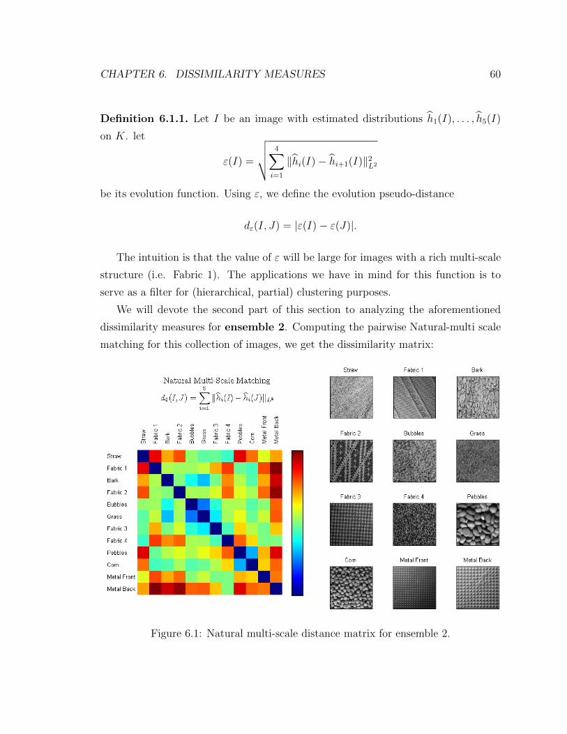
CHAPTER 6. DISSIMILARITY MEASURES 60
Definition 6.1.1. Let I be an image with estimated distributions h1(I), . . . , h5(I)
on K. let
ε(I) =
√√√√ 4∑i=1
‖hi(I)− hi+1(I)‖2L2
be its evolution function. Using ε, we define the evolution pseudo-distance
dε(I, J) = |ε(I)− ε(J)|.
The intuition is that the value of ε will be large for images with a rich multi-scale
structure (i.e. Fabric 1). The applications we have in mind for this function is to
serve as a filter for (hierarchical, partial) clustering purposes.
We will devote the second part of this section to analyzing the aforementioned
dissimilarity measures for ensemble 2. Computing the pairwise Natural-multi scale
matching for this collection of images, we get the dissimilarity matrix:
Figure 6.1: Natural multi-scale distance matrix for ensemble 2.

CHAPTER 6. DISSIMILARITY MEASURES 61
Here, distances decrease (resp. increase) when color goes toward blue (resp. red).
This ensemble serves as a great example of how easy it is for humans to rank similarity
between textures, and then how hard it is to actually identify the criteria involved
in the decision making process. If one takes for example Fabric 3, Metal Front and
Metal Back, then it is clear that the first two are closer together. This is accurately
captured by the v-Invariant and the d4 distance. From the matrix we also get that
Bubbles and Grass are the closest, the second closest pair would be Corn and Pebbles,
while Fabric 1 and Metal Back are the two farthest apart. One would be tempted to
say that Fabric 3 and Metal Front are the closest, but this is only true at large scales,
when one ignores the weave pattern in the fabric.
Using complete linkage, in which two clusters are as similar as their most dissimilar
points, we compute the dendrogram associated to the previous distance matrix:
(a) Complete linkage dendrogram. (b) Resulting Classes.
Figure 6.2: Classes emerging from d4 distance on Ensemble 2.
A natural question that arises is how to use ensemble-specific information and
the v-Invariant, to achieve classifications say by material or natural versus synthetic
textures. We hint now to how variations across scales can be used to this end.

CHAPTER 6. DISSIMILARITY MEASURES 62
We begin by computing the evolution function ε for all images in ensemble 2:
Figure 6.3: Evolution function ε(I) for images in Ensemble 2.
ε provides a natural partition into classes for ensemble 2. Notice that, with the
exception of Plastic Bubbles, all man-made patterns rank above naturally occurring
textures when measured by ε.
The concluding remark from this section, is that the v-Invariant is a simple
and compact representation for images, that allows one to easily compare texture
attributes. The dissimilarity measures presented in this section, can be thought of as
the naive distances coming for free with the definition of the v-Invariant.
How far can one take this representation when looking for purpose-specific dis-
similarity measures? In the next section we treat this question when the goal is to
analyze surface and image rotation.
6.2 Image Rotation
A crucial aspect toward exploiting the full power of an invariant associated to images,
is understanding its behavior under geometric transformations such as translation,
rotation and scaling of the input.
We will show in this section that image rotation has a particularly simple effect on
the distribution of patches on the Klein bottle, as well as a straightforward interpre-
tation in the spectral domain of the v-Invariant. With this interpretation at hand, we
present a mathematical and computational framework for estimating dissimilarities
between images in a rotation invariant a fashion.

CHAPTER 6. DISSIMILARITY MEASURES 63
More specifically, we introduce the R-distance dR as a rotation invariant version
of d4, and through the computational model we show how the rotation factor can
be recovered. We end this section with an SO(2,R)-equivariant version of the v-
Invariant.
6.2.1 Behavior of the v-Invariant under the SO(2,R) action.
Proposition 6.2.1. Let T ∈ SO(2,R) be counter-clockwise rotation by an angle
τ ∈ [−π, π) and let h ∈ L2(K,R). If the coefficients of h and hτ (x, y) = h(x − τ, y)
with respect to the trigonometric basis on K are
a1, . . . , am, bn, cn, dnm, enm, . . . and aτ1, . . . , aτm, b
τn, c
τn, d
τnm, e
τnm, . . .
then
aτm = am ,
[bτn
cτn
]= T 2n
([bn
cn
]),
[dτnm
eτnm
]= T n
([dnm
enm
])for all n,m ∈ N.
Proof. We present the proof for τ ≥ 0, the one for τ < 0 being similar. It follows
from 5.2.3 that
aτm =1
(2π)2
∫ 2π
0
∫ π
0
h(x− τ, y) cos(my)dxdy
=1
(2π)2
∫ 2π
0
∫ π−τ
−τh(x, y) cos(my)dxdy
=1
(2π)2
(∫ 2π
0
∫ π
0
h(x, y) cos(my)dxdy −∫ 2π
0
∫ π
π−τh(x, y) cos(my)dxdy
+
∫ 2π
0
∫ 0
−τh(x, y)cos(my)dxdy
).
If for the second term in the last equation we perform the change of coordinates
(x, y) 7→ (x − π, 2π − y), then using h(x − π, 2π − y) = h(x, y) we conclude that
aτm = am.

CHAPTER 6. DISSIMILARITY MEASURES 64
Following a similar argument we see that
bτn =1
(2π)2
∫ 2π
0
∫ π
0
h(x− τ, y) cos(2n)dxy
=1
(2π)2
∫ 2π
0
∫ π−τ
−τh(x, y)
(cos(2nx) cos(2nτ) + sin(2nx) sin(2nτ)
)dxdy
= bn cos(2nτ) + cn sin(2nτ)
cτn = −bn sin(2nτ) + cn cos(2nτ)
The result follows now by writing these equations using the matrix of T with respect
to the standard basis.
Using the linearity of the expected value, one obtains.
Corollary 6.2.2. Under the hypotheses of the previous proposition, one has that
aτm = am ,
[bτn
cτn
]= T 2n
([bn
cn
]),
[dτnm
eτnm
]= T n
([dnm
enm
])(6.1)
yield unbiased estimators for the coefficients of hτ with respect to the trigonometric
basis on K.
Let us now see how these results apply to image rotation. From the Klein bottle
model (Fig 3.6), it follows that the rotation (with respect to its center) of a contin-
uous approximation I for an image I, has the effect of translating horizontally the
probability density function associated to its small patches . That is h(Iτ ) = hτ (I),
where Iτ is the counter-clockwise rotation of I by an angle τ .
In the discrete case, the local averages taken to form the pixels of the image have
a non-trivial effect on the resulting rotation. Nonetheless, if S = {P1, . . . , PN} ⊆ K
is a sample associated to I, where Pi = (Xi, Yi), then Sτ = {P τ1 , . . . , P
τN} where
P τi = (Xi + τ, Yi), can be regarded a sample drawn from h(Iτ ) and thus can be used
for the coefficient estimation stage in our pipeline. That is, h(Iτ ) = hτ (I).

CHAPTER 6. DISSIMILARITY MEASURES 65
The coefficients computed using this sample coincide with those in equation 6.1,
and thus it makes sense to take them as the v-Invariant at the corresponding scale,
for Iτ . If follows from proposition 6.2.1, that given images I, J and τ ∈ [−π, π) one
can compute φ(I, J, τ) = d4(Iτ , J)2 in terms of v(I), v(J) and τ alone. Let
vk(I) = (ak,1, . . . , ak,m, bk,n, ck,n, dk,nm, ek,nm, . . . , ek,RS)
vk(J) = (a′k,1, . . . , a′k,m, b
′k,n, c
′k,n, d
′k,nm, e
′k,nm, . . . , e
′k,RS)
then
φ(I, J, τ) := d4(Iτ , J)2 (6.2)
=5∑
k=1
‖vk(Iτ )− vk(J)‖2
= ‖v(I)‖2 + ‖v(J)‖2 − 2A(I, J)− 2ϕ(I, J, τ)
where
‖v(I)‖2 =5∑
k=1
‖vk(I)‖2
A(I, J) =5∑
k=1
D∑m=1
ak,ma′k,m
ϕ(I, J, τ) =5∑
k=1
( D0∑n=1
⟨T 2n
[bk,n
ck,n
],
[b′k,n
c′k,n
]⟩+
D∑n+m=1
⟨T n
[dk,nm
ek,nm
],
[d′k,nm
e′k,nm
]⟩)
=D∑n=1
αn cos(nτ) + βn sin(nτ). (6.3)
Combining these formulae and proposition 6.2.1 we get

CHAPTER 6. DISSIMILARITY MEASURES 66
Proposition 6.2.3. For all images I, J and all τ, κ, σ ∈ [−π, π] we have:
1. ‖v(Iτ )‖ = ‖v(I)‖.
2. A(Iτ , Jκ) = A(I, J).
3. ϕ(Iτ , Jκ, σ) = ϕ(I, J, σ + τ − κ).
Definition 6.2.4. Let I, J be images in gray scale. We define the R-distance dR
as
dR(I, J) = minτ∈[−π,π)
d4(Iτ , J). (6.4)
Theorem 6.2.5. The R-distance dR, defines a metric on the set of conjugacy classes
of images under the SO(2,R) action.
Proof. Symmetry of dR follows directly from the formulae in proposition 6.2.3, so let
us show that the triangular inequality holds. To this end, let I, J,K be images and
let τ, κ ∈ [−π, π] be so that
dR(I, J) = d4(Iτ , J) , dR(J,K) = d4(J
κ, K).
Using the formulae from proposition 6.2.3 and the fact that d4 satisfies the triangular
inequality, we conclude that
dR(I, J) + dR(J,K) = d4(Iτ , J) + d4(J
κ, K)
= d4(Iτ+κ, Jκ) + d4(J
κ, K)
≥ d4(Iτ+κ, K)
≥ dR(I,K).

CHAPTER 6. DISSIMILARITY MEASURES 67
6.2.2 Computing the R-distance
In order for dR to be useful in real world image comparisons, it is imperative that we
device a suitable computational scheme. The first thing to notice is that
τ ∗ = argmaxτ∈[−π,π)
ϕ(I, J, τ) (6.5)
if and only if d4(Iτ∗ , J) = dR(I, J). Writing the objective function from 6.5 in terms
of τ as
ϕ(I, J, τ) =D∑n=1
αn cos(nτ) + βn sin(nτ)
where αn, βn depend only on v(I) and v(J) (see equation 6.3), it follows that τ ∗
satisfies the equation
D∑n=1
nβn cos(nτ ∗)− nαn sin(nτ ∗) = 0.
This way, if
q(z) =D∑n=1
(nβn − inαn)zn and q(z) =D∑n=1
(nβn + inαn)zn
then z∗ = eiτ∗
is a root of the degree 2D complex polynomial
p(z) = zD ·(q(z) + q(1/z)
).
The previous analysis can be summarized as follows:
Lemma 6.2.6. Let
p(z) =D∑n=1
n(βn − iαn)zD+n + n(βn + iαn)zD−n
where the αn, βn are given by 6.3. If τ ∗ is a minimizer for 6.4 and z∗ = eiτ∗
then
p(z∗) = 0. Therefore, computing dR(I, J) reduces to minimizing φ(τ) = φ(I, J, τ)

CHAPTER 6. DISSIMILARITY MEASURES 68
(refer to equation 6.2) over the set of arguments from (unitary) roots of p(z).
The roots of p(z) can in principle be computed as the eigenvalues of its companion
matrix. This is how the MATLAB routine roots is implemented. It is known ([10])
that roots produces the exact eigenvalues of a matrix within roundoff error of the
companion matrix of p. This, however, does not mean that they are the exact roots
of a polynomial with coefficients within roundoff error of those of p.
Let p be the monic polynomial having roots(p) as its exact roots. It follows that
p is close to p in a precise sense [1]. Indeed, let ε be the machine precision and let
E = [Eij] be a dense perturbation matrix, where the Eij are small multiples of ε. If
A is the companion matrix of
p(z) = zn + an−1zn−1 + · · ·+ a1z + a0
and p(z) is the characteristic polynomial of A+E, then to first order, the coefficient
of zk−1 in p(z)− p(z) is
k−1∑m=0
am
n∑i=k+1
Ei,i+m−k −n∑
m=k
am
k∑i=1
Ei,i+m−k
where an is defined to be 1.
This result suggests in our case, that even when roots(p) does not return the
exact roots of p, but those of a slight perturbation p, their arguments
Arg(roots(p)
)⊆ [−π, π)
can be used as the initial guess in an iterative approximation, e.g. Newton’s method,
looking to minimize φ(τ). Given that simple expressions for φ′(τ), φ′′(τ) and good
initial points are readily available, one expects a fast convergence in methods based
on gradient descent.
Let
a∗ = GradientDescent(φ, a)
be found in a Newton-type method, looking to minimize φ with a as the starting

CHAPTER 6. DISSIMILARITY MEASURES 69
point. For this step, we use the fminunc routine included in the Statistics MATLAB
Toolbox, which has a fast convergence and high accuracy when provided with φ′′.
The computational scheme for calculating dR(I, J) can be summarized as follows:
Input v-Invariants v(I) and v(J) for I and J .
Output R-distance dR(I, J)minimizer τ ∗ = argmin
τ∈[−π,π)d4(I
τ , J)
1. Determine the polynomial p(z) and the arguments
A =Arg(roots(p)
)2. for each a ∈ A do
a∗ = GradientDescent(φ, a)end
3. Find
τ ∗ = argmina∗∈A∗
φ(a∗)
where A∗ = GradientDescent(φ,A).
Figure 6.4: Computational Scheme for the R-distance dR
6.2.3 A rotation invariant version of v(I)
The version of v(I) that we have in mind is an association
I 7→ v(I)
so that v(I) = v(Iτ0) for some τ0 ∈ [−π, π) depending only on v(I), and so that
v(Iτ ) = v(I) for all τ ∈ [−π, π). This implies that whenever v(I) is rotation invariant,
that is v(I) = v(Iτ ) for all τ ∈ [−π, π), v is given by
v(I) = v(I).

CHAPTER 6. DISSIMILARITY MEASURES 70
For the general case, let us assume that v(I) = [vij] = (v1(I); · · · ; v5(I)) where
vk(I) = (ak,1, . . . , ak,m, bk,n, ck,n, dk,nm, ek,nm, . . . , ek,RS)
is not rotation invariant, so it follows that there exists a nonzero vector of the form[bk,n
ck,n
]or
[dk,nm
ek,nm
].
The first entries of such vectors can be ordered with respect to their position in
v(I) = [vij] by means of (i, j) 7→ (i + j − 1)(i + j − 2)/2 + i, so let vi0j0 be the
smallest of such entries. Let u0 be the corresponding vector, write e1 =
[1
0
]and let
T ∈ SO(2,R) be the clockwise rotation given by
u0‖u0‖
=
T 2n0(e1) if vi0j0 = bk0,n0
T n0(e1) if vi0j0 = dk0,n0m0
If τ0 ∈ [−π, π) is the angle associated to T , then by defining v(I) = v(Iτ0) we get
that I 7→ v(I) has the desired properties.
Remarks:
1. Let I be an image, κ ∈ [−π, π) and let J = Iκ. An important aspect of the
ideas presented in this section, is how simple it becomes to estimate κ (up to
self-similarities of I) from v(I) and v(J). Indeed, if τ0(I) ∈ [−π, π) is so that
v(Iτ0(I)) = v(I) then
κ ≡ τ0(I)− τ0(J) mod 2π.
In the case where J is not exactly the result of rotating I, e.g. when I and
J are images of the same object under different lightning conditions and view
point, the minimizer computed in figure 6.4 serves as a generalization of κ.
In order to deal with the non-uniqueness of the minimizer, a natural choice is

CHAPTER 6. DISSIMILARITY MEASURES 71
to require τ ∗ to be the one with the smallest absolute value.
2. Recall the definition of d4(I, J) as the quantity
d4(I, J) =
√√√√ 5∑i=1
‖vi(I)− vi(J)‖2
where v(I) = (v1(I); . . . ; v5(I)). If we write v(I) = (v1(I); . . . ; v5(I)) then we
can define a rotation invariant version of d4 by the formula
d4(I, J) =
√√√√ 5∑i=1
‖vi(I)− vi(J)‖2
from which it follows that
d4(I, J) = d4(Iτ0(I), Jτ0(J))
= d4(Iτ0(I)−τ0(J), J)
≥ minτ∈[−π,π)
d4(Iτ , J)
= dR(I, J)
Even when d4 is fairly simple to compute in comparison to dR, the best classi-
fication results were obtained with the latter.
3. Recall the evolution function ε defined as
ε(I) =
√√√√ 4∑i=1
‖vi(I)− vi+1(I)‖2
It follows from this formula and proposition 6.2.1 that ε is rotation invariant.
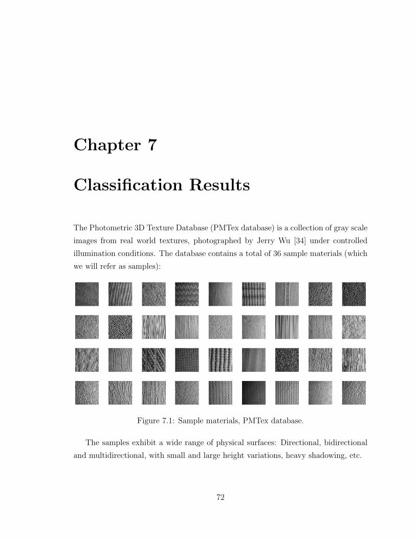
Chapter 7
Classification Results
The Photometric 3D Texture Database (PMTex database) is a collection of gray scale
images from real world textures, photographed by Jerry Wu [34] under controlled
illumination conditions. The database contains a total of 36 sample materials (which
we will refer as samples):
Figure 7.1: Sample materials, PMTex database.
The samples exhibit a wide range of physical surfaces: Directional, bidirectional
and multidirectional, with small and large height variations, heavy shadowing, etc.
72

CHAPTER 7. CLASSIFICATION RESULTS 73
Each sample is then captured under different poses and illumination conditions:
Figure 7.2: Instances of a sample in the PMTex database.
The different poses of the sample correspond to counterclockwise rotations of the
material, with respect to the texture plane. The resulting positions are of the formiπ6
where i = 0, . . . , 6. The rotation of the light source, which is located with a slant
of π4
at a fixed distance from the center of the material, occurs in increments of π/4
or π/2. This yields a database of 1930 texture images, which we will analyze in this
chapter.
7.1 Material Categories Via Hausdorff Distance
From an appearance-based viewpoint, categories of materials emerge naturally when
textural properties of pairs of samples under varying lighting conditions and camera
pose, are used as a measure of similarity. In particular, samples can be categorized by
the way in which their textural information changes when seen from different angles.
As an example to fix ideas, woolen sweaters knitted in different patterns may
present fairly different textural information, while the way in which the two textures
change with varying lighting conditions is often very similar. We propose the Haus-
dorff distance between collections of sample instances, as a way of comparing this
changes in textural information.
Let S be a sample (e.g. a piece of wood, fabric, terrain, etc) for which images
S1, . . . , Sn taken under several lighting conditions and camera poses, are available.
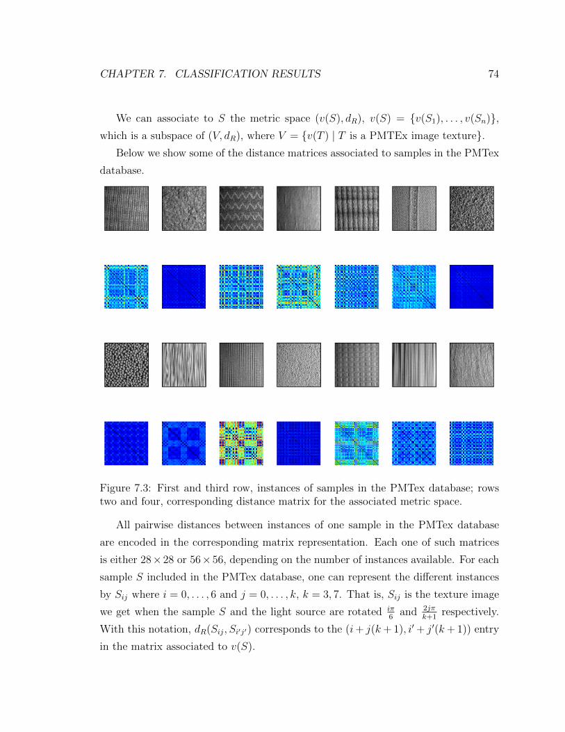
CHAPTER 7. CLASSIFICATION RESULTS 74
We can associate to S the metric space (v(S), dR), v(S) = {v(S1), . . . , v(Sn)},which is a subspace of (V, dR), where V = {v(T ) | T is a PMTEx image texture}.
Below we show some of the distance matrices associated to samples in the PMTex
database.
Figure 7.3: First and third row, instances of samples in the PMTex database; rowstwo and four, corresponding distance matrix for the associated metric space.
All pairwise distances between instances of one sample in the PMTex database
are encoded in the corresponding matrix representation. Each one of such matrices
is either 28×28 or 56×56, depending on the number of instances available. For each
sample S included in the PMTex database, one can represent the different instances
by Sij where i = 0, . . . , 6 and j = 0, . . . , k, k = 3, 7. That is, Sij is the texture image
we get when the sample S and the light source are rotated iπ6
and 2jπk+1
respectively.
With this notation, dR(Sij, Si′j′) corresponds to the (i+ j(k+ 1), i′+ j′(k+ 1)) entry
in the matrix associated to v(S).

CHAPTER 7. CLASSIFICATION RESULTS 75
Remark: The regularity in the patterns observed in figure 7.3, serves as strong
evidence of the robustness of our method to sampling effects when computing v(Sij),
and numerical errors when calculating dR. The idea we explore in this section, is the
extent to which these patterns serve as fingerprints for material samples.
Understanding how the scale of colors reflects distance between textures in the
PMTex database, is perhaps easier when looking at the distance metric representing
(V, dR). We include it below:
Figure 7.4: 1930-by-1930 distance matrix representing (V, dR). All matrices in figure7.3 are present as diagonal blocks of this one.

CHAPTER 7. CLASSIFICATION RESULTS 76
Using the Hausdorff distance we define the M -distance dM (M for material clas-
sification) as:
Definition 7.1.1. Given samples S, S ′ with texture images S1, . . . , Sn and S ′1, . . . , S′m
taken under distinct lighting conditions and camera poses, we let
dM(S, S ′) = dH(v(S), v(S ′))
= max{
maxi
minjdR(Si, S
′j),max
jminidR(Si, S
′j)}.
The material categories should emerge now as clusters, with distance measured
by dM . We use complete clustering, in which two clusters are as similar as their most
dissimilar elements, and report the obtained classes.
Figure 7.5: Material categorization from Hausdorff distance.
The corresponding dendrogram follows.

CHAPTER 7. CLASSIFICATION RESULTS 77
Figure 7.6: Complete-linkage dendrogram for dM
7.2 Texture Classification From Known Instances
It is often the case that instances from families of textures are readily available for
classification purposes. The categorization power of an invariant and its associated
dissimilarity measures, can then be gauged through classification of novel instances.
In this machine-learning framework, the first step is to randomly select a subset of
instances for each sample in the PMTex database. Using the resulting training set,
we categorize the remaining texture images via nearest neighbor for each one of the
distances introduced in 6.2. We now describe the details:
1. First, we choose a percentage 0 < p ≤ 100, which will determine the size of the
training set.
2. For each sample S in the PMTex database we do the following: let S1, . . . , Sn
be the instances available for S (n will be either 28 or 56), and let k =⌊p∗n100
⌋.

CHAPTER 7. CLASSIFICATION RESULTS 78
Randomly choose an order preserving, injective function
σ : {1, . . . , k} −→ {1, . . . , n}
and let Tp(S) = {Sσ(1), . . . , Sσ(k)}.
3. Let
Tp =⋃S
Tp(S)
where the union is taken over all samples in the PMTex database. Tp will
be regarded as a random training set for the percentage p. The set of novel
instances to be classified is now Np =⋃S
({S1, . . . , Sn} − Tp(S)
).
4. For each S ∈ Np, let S ′ ∈ Tp be the closest element in Tp as measured by
d ∈ {d4, dR, d4}. If S and S ′ are instances of the same sample, we will deem the
classification as successful. The classification success of d in (Tp, Np) can now
be computed as the percentage
successful classifications
|Np|∗ 100.
We repeat this process on 1, 000 random training sets, for different percentages
p = 7, 14, 25, 50. The mean and standard deviation of classification success, are then
computed for each distance. We compare in figure 7.7, the classification success of d4,
dR and d4 at p = 7, 14, 25, 50. Nodes in the plot correspond to the computed mean
at the given percentage, and the error bars to the standard deviation.
To have an idea of the numbers, we show in table 7.1 the sizes of Tp and Np as
functions of p.
Table 7.1: |Tp| and |Np| as functions of pp 7 14 25 50|Tp| 135 270 482 965|Np| 1,750 1,660 1,448 965

CHAPTER 7. CLASSIFICATION RESULTS 79
With 36 samples on the PMTex database and at least 28 instances per sample, the
number of possible training sets for each value of p is grater than(2814
)36 ≥ 4× 10252.
While the number of randomly generated training sets (per value of p) is only 103,
the small variance in computed success percentage, strengthes the validity of our
estimation.
Figure 7.7: Classification success of d4, dR and d4 on the PMTex database. We selectp% instances per sample as training set, and classify novel textures using nearestneighbors. The error-bar plot shows the mean and standard deviation of the classifi-cation success, using 1,000 random training sets.
The classification success of dR is, as expected, grater than that of d4 and d4
on the PMTex database. This comparison makes the case for the importance of
understanding the behavior of image invariants with respect to image transformations.

CHAPTER 7. CLASSIFICATION RESULTS 80
We have only scratched the surface with respect to actions of the general linear
group GL(3,R). Scaling can be taken into consideration with distances like d1 (refer
to section 6.1), while the study of shear mappings could shed light on the effects of
3D motion and perspective. Is it worth noticing how the mathematical framework for
distributions of high contrast patches (thought of as functions on a meaningful space
like the Klein bottle, and efficiently represented by Fourier-like coefficients), allows
one not only to interpret, but to quantify the changes in the representation.
A success rate of almost 97% via nearest neighbor implies a little bit more than
good classification power. It shows that the notion of similarity being used, is an
adequate local approximation to the intrinsic distance. In this sense, it shows that
the local behavior of (V, dR), can be used to infer global information of how the image
of the v-Invariant (as a function from images to coefficients) sits inside R42. In the
next section, we will present a construction pursuing this goal.
7.3 Local to Global Information: Intrinsic distance
reconstruction and Class Partitioning
As discussed in the previous section, the local information carried by the v-Invariant
and the R-distance, is well suited for texture classification and class partitioning. The
main issue with distances which are estimated or defined following certain heuristics,
is that they often fail at capturing more than the local behavior. It is exactly the same
difficulty one runs into when trying to measure distances in an embedded manifold
using the ambient metric, as opposed to the geodesic distance. If we look for example
at figures 7.3 and 7.4, we will see that dR suffers of this drawback. On the one hand,
figure 7.3 and the previous section suggest that it handles local distances accurately;
while on the other hand, figure 7.4 clearly shows that dR by itself does not do a very
good job at separating instances of the same sample when lighting conditions are
varied. We propose in this section a local to global approach based on nearest neighbor
graphs, in order to recover the intrinsic distance. See [28] for other applications of
this idea.
CHAPTER 7. CLASSIFICATION RESULTS 81
Recall that a path from a to b in a directed graph G, is a sequence of vertices
g0, . . . , gN so that g0 = a, gN = b and (gi−1, gi) is an edge in G for all i = 1, . . . , N .
The length of such path is defined to be N . We say that there is a loop in G containing
the vertices a,b if there are paths from a to b and from b to a.
Notice that
“either a = b, or a and b are in a loop”
defines an equivalence relation on the set of vertices of G, and the equivalence classes
are referred to as the strongly connected components of G. There is a natural distance
in G arising from this data. Indeed, if a 6= b are in the same strongly connected
component, we define dG(a, b) as one half of the length of the shortest loop containing
them. If a = b we let dG(a, b) = 0 and if a, b are not in a loop in G, we let dG(a, b) =∞.
Given a finite metric space (X, dX) and k ∈ N, one can associate a directed graph
Gk(X) = Gk(X, dX) with vertex set X, and where an edge is drawn from x to y if
y 6= x falls within the k-th nearest neighbors of x. The idea we exploit in this section,
is that the strongly connected components of Gk(V ) = Gk(V, dR) should recover the
sets of instances of samples in the PMTex database. The extent to which this is true,
can be measured using the separation of classes under the graph distance.
Let us denote by dk the distance associated to the directed graph Gk(V ), and
replace dk by min(dk, 20). These two metrics are equivalent in the sense that they
induce the same topology, but the second is more suitable for computations and
comparisons. We will denote the finite metric, by abuse of notation, also as dk.
Given that each class within the PMTex database gets connected at a potentially
different rate as we go from Gk(V ) to Gk+1(V ), then the choice of a particular value of
k is somewhat arbitrary and unmotivated. To see this, compare the distance matrices
in figure 7.3. Another observation in this regard, is that it should be more meaningful
to look at the evolution of dk as k increases, to rule out “false” edges and give a better
estimate of the global distance.
In order to overcome these difficulties, three ideas will guide our approach: First,
we deem distances between elements as more relevant, if they do not change too
much as the graph gets more connected. The second observation is that for each

CHAPTER 7. CLASSIFICATION RESULTS 82
class, there is a range of values of k in which inner-class distances do not change too
much. This, due to the fact that edges are being drawn namely between elements
from the same class. The third and final observation is that, as suggested by figure
7.7, the stabilization occurs as the class approach full connectedness.
Based on these observations, we propose a weighted average of the distances
d1, . . . , dN as an approximation to the intrinsic distance. We let N = 20 as this
value is roughly half the size of all classes in the PMTex database. We define
d =1
210(d1 + 2d2 + 3d3 + · · ·+ 20d20)
and the distance matrix corresponding to (V, d) is now
Figure 7.8: 1930-by-1930 distance matrix for (V, d). Each diagonal block in dark bluerepresents a class in the PMTex database.

CHAPTER 7. CLASSIFICATION RESULTS 83
By comparing this matrix to the one on figure 7.4, one can see how the intrinsic
metric does a much better job at separating between classes in the PMTex database.
Each diagonal block in dark blue, represents the distances between all instances of
a given texture sample. The conclusion we can draw from this analysis, is that
the strongly connected components from nearest neighbor graphs, were in this case
successful at recovering the initial texture classes.

Chapter 8
Conclusions and Final Remarks
The application of Gabor filters for feature extraction, the maximum response 8
(MR8) filters for texture analysis, and the use of the Discrete Cosine Transformation
(DCT) in image compression, are all closely related approaches. They all attempt to
project small patches onto a finite number of more basic ones, and probe the result in
order to extract meaningful information. This strategy is an old, and very successful
one.
Projecting onto the Klein bottle follows this idea with two new features built in.
First, the actual domain of filters (the Klein bottle) is continuous, which increases
the fidelity of the filtered data. Notice that better accuracy in the feature extraction
stage does not become an obstacle for compact representation, for two numbers are
enough. Second, by taking into account the actual statistical and geometric structure
of the space of optical patches, one gains insight into phenomena and applications that
were hidden before having the model. Just as the description of distributions of high
contrast patches from an image, and the effect of rotation became quite apparent
having the model at our disposal, many more uses of this structure are yet to be
discovered.
The idea of describing a patch as a point on a Klein bottle works for all images. In
this paper we used an statistical approach to study images whose statistic properties
capture most of the information available. It would be interesting to explore other
ways of using this representation.
84

CHAPTER 8. CONCLUSIONS AND FINAL REMARKS 85
The results presented here are encouraging as seen from the texture analysis and
classification viewpoint: On the one hand, the Fourier representation proved to be
compact and powerful for discrimination purposes. On the other hand, it is important
to notice that we only used (purely) linear and quadratic information from the patches
we selected. It would be an interesting direction for future research to enlarge the
Klein bottle model, in order to include patches which are frequently encountered in
texture images, and contain higher order information.

Appendix A
Proof of theorem 5.2.2
Since 〈·, ·〉K is readily a positive definite Hermitian form, we will proceed to check the
orthogonality relations, the convergence assertion and the completeness statement.
Let δij be the Kroeneker delta function. That is, δij = 1 if i = j and zero otherwise.
Notice that for n, n′ ∈ Z and m,m′ ∈ N ∪ {0} we have
(2π)2δnn′δmm′ = (2π)2〈einx, ein′x〉S1 · 〈eimy, eim′y〉S1
=
∫ 2π
0
ei(n−n′)xdx ·
∫ 2π
0
ei(m−m′)ydy
=
∫ 2π
0
(∫ π
0
+
∫ 2π
π
einx+imy · e−in′x−im′ydx)dy
=
∫ 2π
0
∫ π
0
einx+imy · e−in′x−im′ydxdy +∫ 0
−2π
∫ π
0
(−1)neinx−imy · (−1)n′e−in
′x+im′ydxdy
=
∫ 2π
0
∫ π
0
ei(n−n′)x+i(m−m′)y + (−1)n−n
′ei(n−n
′)x−i(m−m′)ydxdy.
86

APPENDIX A. PROOF OF THEOREM 5.2.2 87
On the other hand,∫ 2π
0
∫ π
0
((−1)n
′ei(m+m′)y + (−1)ne−i(m+m′)y
)ei(n−n
′)xdxdy
=
(πδnn′ + (δnn′ − 1)
1− (−1)n−n′
(n− n′)i
)∫ 2π
0
ei(m+m′)y(−1)n′+ e−i(m+m′)y(−1)ndy
=
(πδnn′ + (δnn′ − 1)
1− (−1)n−n′
(n− n′)i
)2πδmm′
((−1)n
′+ (−1)n
)
= (−1)n(2π)2δnn′δm0δ0m′
and adding the derived equalities we get
〈φnm, φn′m′〉K = δnn′(δmm′ + (−1)nδm0δ0m′)
which implies the orthogonality relations.
Let us now check the convergence assertion. Let q : S1×S1 −→ K be the quotient
map induced by the equivalence relation (x, y) ∼ (x′, y′) if and only if x− x′ = π and
y + y′ = 0. Then q induces a map
q∗ : M(K,C) −→M(S1 × S1,C)
give by q∗(f) = f ◦ q, and it follows that for each (y, f) ∈ S1 × L2(K), we have a
function fy ∈M(S1,C) given by fy(x) = q∗(f)(x, y).

APPENDIX A. PROOF OF THEOREM 5.2.2 88
The first thing to notice is that if f, g ∈ L2(K) then
〈f, g〉K =1
(2π)2
∫ 2π
0
∫ π
0
f(x, y)g(x, y)dxdy
=1
2(2π)2
∫ 2π
0
∫ π
0
f(x, y)g(x, y)dxdy +
1
2(2π)2
∫ 0
−2π
∫ 2π
π
f(x+ π,−y)g(x+ π,−y)dxdy
=1
2(2π)2
∫S1×S1
q∗(f) · q∗(g) d(τ × τ)
so in particular
‖f‖2K =1
4π
∫ 2
0
‖fy‖2S1dy <∞
which shows that fy ∈ L2(S1) for almost every y ∈ S1. This way, by theorem 5.2.1,
we conclude that
limN→∞
∥∥∥fy − SN(fy)∥∥∥S1
= 0 and ‖fy‖2S1 =∑|fy(n)|2
for almost every y in S1. Notice that
SN(f−y)(x+ π) =N∑
n=−N
1
2π
∫ 2π
0
q∗(f)(τ,−y)e−inτdτ · (−1)neinx
=N∑
n=−N
1
2π
∫ π
−πq∗(f)(τ, y)e−inτdτ · einx
=N∑
n=−N
fy(n)einx
so as a function of two variables, SN(fy)(x) ∈ L2(K).
APPENDIX A. PROOF OF THEOREM 5.2.2 89
An application of Young’s inequality with exponent 2 shows that
1
2
∥∥∥f − N∑m=0
N∑n=−N
f(n,m)φn,m
∥∥∥2K≤
∥∥∥f − SN(fy)∥∥∥2K
+∥∥∥SN(fy)−
N∑m=0
N∑n=−N
f(n,m)φn,m
∥∥∥2K
(A.1)
where
‖f − SN(fy)‖2K = 〈f − SN(fy), f − SN(fy)〉K
=1
2(2π)2
∫ 2π
0
∫ 2π
0
|fy(x)− SN(fy)(x)|2dxdy
=1
2π
∫ 2π
0
1
2‖fy − SN(fy)‖2S1dy
1
2‖fy − SN(fy)‖2S1 ≤ ‖fy‖2S1 + ‖SN(fy)‖2S1
= ‖fy‖2S1 +N∑−N
|fy(n)|2 ≤ 2‖fy‖2S1 .
Since the function y 7→ ‖fy‖2S1 is integrable, Lebesgue’s dominated convergence
theorem implies that limN→∞
‖f − SN(fy)‖K = 0.
To see that the second term in the right hand side of inequality A.1 also goes to
zero as N goes to infinity, notice that
‖φnm‖2K = 1 + (−1)nδm0 and f(n,m)‖φnm‖2K = 〈f, φnm〉K
imply that f(n,m) can be computed as
f(n,m) =(
1− 1
4δm0(3− (−1)n)
)〈f, φnm〉K .

APPENDIX A. PROOF OF THEOREM 5.2.2 90
Thus, for each n ∈ Z
N∑m=0
f(n,m)φnm · e−inx =(1 + (−1)n)
2〈f, φn0〉K +
N∑m=1
〈f, φnm〉K(eimy + (−1)ne−imy
)where
(2π)2〈f, φnm〉K =
∫ 2π
0
∫ π
0
f(x, y)(e−inx−imy + e−in(x−π)+imy)dxdy
=
∫ 2π
0
∫ π
0
f(x, y)e−inx−imydxdy +
∫ 0
−2π
∫ 2π
π
j∗f(x, y)e−inx−imydxdy
= 2π
∫ 2π
0
fy(n)e−imydy = (2π)2fy(n,m).
Since this can also be computed as
〈f, φnm〉K =1
2(2π)2
∫ 2π
0
∫ 2π
0
j∗(f)(x, y)(e−inx−imy + (−1)ne−inx+imy
)dxdy
=fy(n,m) + (−1)nfy(n,−m)
2
we conclude that
N∑m=0
f(n,m)φnm · e−inx =N∑
m=−N
fy(n,m)eimy = SN(fy(n)).

APPENDIX A. PROOF OF THEOREM 5.2.2 91
Now, from the previous calculation and the orthogonality relations in L2(S1)
∥∥∥SN(fy)−N∑
n=−N
N∑m=0
f(n,m)φnm
∥∥∥2K
=1
2(2π)2
∫ 2π
0
∫ 2π
0
∣∣∣ N∑n=−N
(fy(n)−
N∑m=0
f(n,m)(eimy + (−1)ne−imy))einx∣∣∣2dxdy
=N∑
n=−N
1
4π
∫ 2π
0
∣∣∣fy(n)− SN(fy(n))∣∣∣2dy
=1
2
N∑n=−N
∥∥∥fy(n)− SN(fy(n))∥∥∥2S1.
Since for all N,N ′ ∈ N
∑|n|≥N
1
4π
∫ 2π
0
∣∣∣fy(n)− SN ′(fy(n)
)∣∣∣2dy≤
∑|n|≥N
1
2π
∫ 2π
0
|fy(n)|2 + |SN ′(fy(n)
)|2dy
=∑|n|≥N
1
2π
∫ 2π
0
|fy(n)|2dy +∑|n|≥N
‖SN ′(fy(n)
)‖2S1
≤∑|n|≥N
1
2π
∫ 2π
0
|fy(n)|2dy +∑|n|≥N
‖fy(n)‖2S1
=1
π
∑|n|≥N
∫ 2π
0
|fy(n)|2dy
and for almost every y ∈ S1
limN→∞
∑|n|≤N
|fy(n)|2 = ‖fy‖2S1
then by Lebesgue’s dominated convergence theorem, given ε > 0, we can pick N0 ∈ N

APPENDIX A. PROOF OF THEOREM 5.2.2 92
so that for all N ∈ N
∑|n|≥N0
1
4π
∫ 2π
0
∣∣∣fy(n)− SN(fy(n)
)∣∣∣2dy < ε.
This way
limN→∞
N∑n=−N
1
4π
∫ 2π
0
∣∣∣fy(n)− SN(fy (n))∣∣∣2dy≤ 1
2
∑|n|≤N0
limN→∞
∥∥∥fy(n)− SN(fy(n)
)∥∥∥2S1
+ ε
= ε
and since this is true for all ε > 0, letting it go to zero we get the result.
Bibliography
[1] A. Edelman and H. Muralami, Polynomial Roots From Companion Matrix
Eigenvalues, Mathematics of Computation, Vol. 64, No. 210 (Apr., 1995), pp.
763-776.
[2] A. Hatcher, Algebraic Topology, Cambridge University Press, Cambridge, 2002.
[3] A. Lee, K. Pedersen and D. Mumford, The Nonlinear Statistics of High-
Contrast Patches in Natural Images, International Journal of Computer Vision
54(1/2/3), 2003, pp. 83-103.
[4] A. Zomorodian and G. Carlsson, Computing Persistent Homology, Discrete and
Computational Geometry, 33, (2), pp. 247-274.
[5] B. A. Olshausen and D. J. Field, Natural Image Statistics and Efficient Coding,
Network: Comput. Neural Syst., (7), 1996, pp. 333-339.
[6] B. Julesz, Visual Pattern Discrimination, IRE Transactions on Information
Theory, 8, 1962, pp 84-92.
[7] B. Julesz, Textons, the Elements of Texture Perception, and their Interactions,
Nature, 290, (5802), pp. 91-97.
[8] B. W. Silverman, Density Estimation for Statistics and Data Analysis,
[9] C. Borsuk, On the Imbedding of Systems of Compacta in Simplicial Complexes,
Fund. Math., 35, 1948, pp. 217-234.
93
BIBLIOGRAPHY 94
[10] C. Moler, Cleve’s corner: ROOTS-Of polynomials, that is, The MathWorks
Newsletter, vol. 5, no. 1 (Spring 1991), pp. 8-9.
[11] D. Attali and A. Lieutier, Reconstructing Shapes With Guarantees by Unions
of Convex Sets, Archive Hal, hal-00427035, 2009.
[12] D. Attali, H. Edelsbrunner and Y. Mileyko, Weak Witnesses for Delaunay Tri-
angulations of Submanifolds, Proceedings of the 2007 ACM symposium on Solid
and physical modeling, 2007, pp. 143-150.
[13] D. H. Hubel and T. N. Wiesel, Receptive Fields and Funtional Architecture of
Monkey Straite Cortex, J. Physiol. (1), 195, 1968, pp. 215-243.
[14] D. J. Field, Relations Between the Statistics of Natural Images and the Response
Properties of Cortical Cells, J. Opt. Soc. Am., A (4), 1987, pp. 2379-94.
[15] D. L. Cohn, Measure Theory, Birkhauser, 1980.
[16] D. L. Ruderman, The Statistics of Natural Images, Network: Comput. Neural
Syst., (5), 1994, pp. 517-48.
[17] D. Marr, Vision, A Computational Investigation into the Human Representation
and Processing of Visual Information
[18] F. Chazal and S. Y. Oudot, Towards Persistence-Based Reconstruction in Eu-
clidean Spaces, Proceedings of the twenty-fourth annual symposium on Com-
putational Geometry, 2008, pp. 232-241.
[19] G. Carlsson, Topological and Data, Bulletin of the American Mathematical So-
ciety, (46), 2, 2009, pp. 255-308.
[20] G. Carlsson and T. Ishkhanov, A Topological Analysis of the Space of Natural
Images, preprint, (2007).
[21] G. Carlsson, T. Ishkhanov, V. de Silva and A. Zomorodian, On the Local Be-
havior of Spaces of Natural Images, International Journal of Computer Vision,
(76), 1, 2008, pp. 1-12.
BIBLIOGRAPHY 95
[22] G. S. Watson, Density Estimation by Orthogonal Series, The Annals of Math-
ematical Statistics, (40), 4, 1969, pp. 1496-1498.
[23] G. Singh, F. Memoli and G. Carlsson, Topological Methods for the Analysis of
High Dimensional Data Sets and 3D Object Recognition, Point Based Graphics
2007, Prague, September 2007.
[24] G. Singh, F. Memoli, T. Ishkhanov, G. Carlsson, G. Sapiro and D. Ringach,
Tological Structure of Population Activity in Primary Visual Cortex, Journal of
Vision, (8), 8, 2008, pp. 1-18.
[25] H. Edelsbrunner and J. Harer, Persistent Homology - A Survey, Contemp.
Math., 453, 2007, pp. 257-282.
[26] H. Edelsbrunner, D. Letscher and A. Zomorodian, Topological Persistence and
Simplification, Discrete and Computational Geometry, 28, 2002, pp. 511-533.
[27] H. Federer, Curvature Measures, Transactions of the American Mathematical
Society, 54, 1993, pp. 357-386.
[28] J. B. Tenenbaum, V. de Silva and J.C. Langford, A Global Geometric Frame-
work for Nonlinear Dimensionality Reduction, Science, (290), 2000 (December),
pp. 2319-2323.
[29] J. C. Hausmann, On the Vietoris-Rips Complexes and a Cohomology Theory
for Metric Spaces, Prospects in topology, Ann. of Math. Stud., 138, pp. 175-188,
Princeton Univ. Press, Princeton, NJ, 1995.
[30] J. D. Boissonnat, L. J. Guibas and S. Y. Oudot, Manifold Recontructiion in
Arbitrary Dimensions Using Witness Complexes, Proc. 23rd ACM Sympos. on.
Comput. Geom., 2007.
[31] J. G. Dumas, F. Heckenbach, B. D. Saunders and V. Welker, Computing Simpli-
cial Homology Based on Efficient Normal Form Algorithms, In Proc. Integration
of Algebra and Geometry Software Systems, 2002. To be published.

BIBLIOGRAPHY 96
[32] J. H. van Hateren and A. van der Schaaf, Independent Component Filters of
Natural Images Compared with Simple Cells in Primary Visual Cortex, Proc.
R. Soc. Lond., 1998, B (265), pp. 359-366.
[33] J. J. Atick, Could Information Theory Provide an Ecological Theory of Sensor
Proecessing?, Network: Comput. Neural Syst., (3), 1992, pp. 213-51.
[34] Jerry Wu’s PMTex database, available at:
http://www.taurusstudio.net/research/pmtexdb/index.htm
[35] M. Kahle and E. Meckes, Limit Theorems for Betti Numbers of Random Sim-
plicial Complexes, Preprint in arXiv1009.4130v3, January 18th 2011.
[36] M. Reed and B. Simon, Methods of Modern Mathematical Physics, VOL I,
Academic Press Inc, 1980.
[37] M. Tarter and R. Kronmal, On Multivariate Density Estimates Based on Or-
thogonal Expansion, The Annals of Mathetmatical Statistics, (41), 2, 1970, pp.
718-722.
[38] M. Varma and A. Zisserman, A Statistical Approach to Material Classification
Using Image Patch Exemplars, IEEE Transactions on Pattern Analysis and
Machine Inteligence, (31), 11, 2009 (November), pp. 2032-2047.
[39] N. Amenta and M. Bern, Surface Reconstruction by Voronoi Filtering, Discrete
Computational Geomtry, 22, 1999, pp. 481-504.
[40] N. Amenta, M. Bern and D. Eppstein, The Crust and the β-Skeleton: Com-
binatorial Curve Reconstruction, Graphical Modelsand Image Processing, 60,
1998, pp. 125-135.
[41] P. Brodatz, Textures: A Photographic Album for Artists and Designers, Dover
Publications, August 20, 1999.
[42] P. Niyogi, S. Smale and S. Weinberger, Finding the Homology of Submanifolds
with High Confidence from Random Samples, Discrete and Computational Ge-
ometry, 39, (1-3), 2008, pp. 419-141.

BIBLIOGRAPHY 97
[43] R. Miller, Discussion of Projection Pursuit, Annals of Statistics, (13), 2, 1985,
pp. 510-513.
[44] S. Lang, Algebra, Third edition, Springer-Verlag, 2002.
[45] S.Y. Oudot, On the Topology of Restricted Delaunay Triangulation and Witness
Complex in Higher Dimensions, Preprint, November 2006.
[46] USC-SIPI Texture database, available at:
http://sipi.usc.edu/database/database.cgi?volume=textures
[47] V. de Silva, A Weak Characterization of the Delaunay Triangulation, Geome-
triae Dedicata, (1), 135, 2008, pp. 39-64.
[48] V. de Silva and G. Carlsson, Topological Estimation Using Witness Complexes,
In Eurographics Symposium on Point-Based Graphics, ETH, Zurich, Switzer-
land, 2004.
[49] V. de Silva and R. Ghrist, Coverage in Sensor Networks Via Persistent Homol-
ogy, Algebraic & Geomtric Topology, 7, 2007, pp. 339-358.
[50] Y. Katznelson, An Introduction to Harmonic Analysis, Third edition, Cam-
bridge University Press, 2004.