Ludwig-Maximilians-Universitat Munchen

Prof. Dr. Thomas Vogel

Lecture in the winter term 2017/18

Topology 1

Please note: These notes summarize the content of the lecture, many details andexamples are omitted. Sometimes, but not always, we provide a reference for proofs,examples or further reading. I will not attempt to give the first reference where atheorem appeared. Some proofs might take two lectures although they appear in asingle lecture in these notes. Changes to this script are made without further noticeat unpredictable times. If you find any typos or errors, please let me know.

1. Lecture on Oct. 16 - Basic notions from point set topology

• Reference: Chapter 1 in [Ja]• Definition: Let X be a set. A topology on X is a subset T ⊂ {subsets of X} =P (X) such that

– ∅, X ∈ T ,– U, V ∈ T implies U ∩ V ∈ T , and– Ui ∈ T for i ∈ I (I is some index set) implies (∪iUi) ∈ T .

A set U ∈ T is called open. A ⊂ X is closed if X \ A is open.• Examples: T = {∅, X} and P (X) are topologies. If (X, d) is a metric space,

then

Td = {U ⊂ X | for all u ∈ U there is δ > 0 such that Bδ(u) ⊂ U}is a topology. Here Bδ(u) = {v ∈ X | d(u, v) < δ} is the δ-ball around u.• Definition: A topological space (X, T ) is Hausdorff if for all u 6= v there are

open sets U 3 u and V 3 v such that U ∩ V = ∅. It is connected if for allU, V ∈ T such that U ∪ V = X and U ∩ V = ∅ it follows that U = ∅ or V = ∅.

A subset U ⊂ T is an open cover of X if ∪U∈UU = X. X is compact iffor every open cover U there is a finite collection U1, U2, . . . , Un ∈ U such thatU1 ∪ . . . ∪ Uk = X.• Examples: Every topology which is induced by a metric is Hausdorff. [0, 1] is

compact and connected in the standard topology (i.e. the one induced by themetric d(x, y) = |x− y|).• Proof: Hausdorff is clear. For U, V open and disjoint in [0, 1] such that U∪V =

[0, 1] assume 0 ∈ U and V 6= ∅ consider x0 = sup{t | [0, t) ⊂ U}. Then x0 6∈ Ubut x0 ∈ V leads to a contradiction to the choice of x0.

In order to show that [0, 1] is compact we show the following: If U is an opencover of [0, 1], then there is δ > 0 such that

∀x ∈ [0, 1]∃U ∈ U : (x− δ, x+ δ) ∩ [0, 1] ⊂ U.

If this is not true, then there is a sequence xn such that (xn−1/n, xn+1/n) 6⊂ Ufor all U ∈ U . But (xn) has a convergent subsequence because [0, 1] is boundedan complete. The limit point of such a subsequence lies in one set UU . Thisleads to a contradiction to the choice of the sequence (xn). Using δ one canextract a finite subcover from U .

2

• Definition: Let (X, TX) and (Y, TY ) be topological spaces and f : X −→ Y amap. f is continuous if for all V ∈ TY the set f−1(V ) is open in X.• Theorem (Heine-Borel): A set K ⊂ Rn with the topology induced by the

Euclidean distance is compact if it is closed and bounded.• Remark: When TX and TY are induced by metrics, then this definition is

equivalent to the ε-δ-definition of continuity.• Definition: Let A ⊂ (X, T ). Then one defines the subspace topology on A by

TA = {V ⊂ A | there is U ∈ T such that U ∩ A = V }.This is the smallest topology on A for which the inclusion map i : A ↪→ X iscontinuous.• Definition: Let ∼ be an equivalence relation on (X, T ). Then the quotient

topology on X/ ∼ is

T∼ = {V ⊂ X/ ∼ | pr−1(V ) ∈ T }where pr : X −→ X/ ∼ is the quotient map. The quotient topology is thelargest topology for which pr is continuous.• Lemma: If (X, T ) is compact and A ⊂ X is closed, then A is compact.• Proof: If V ⊂ TA is an open cover of A, then for all V ∈ V there is U(V ) ∈ T

such that U(V ) ∩A = V . Then {U(V ) |V ∈ V} ∪ {X \A} is an open cover ofX. From the compactness we get a finite subcover of X and from that a finitesubcover of A.

2. Lecture on Oct. 19 - Basic notions from point set topology

• Lemma: Let K be compact, X any topological space and f : K −→ Xcontinuous. Then f(K) is compact (viewed as subspace of X).• Proof: An from an open cover of f(K) we obtain an open cover of K.• Proposition: Let X be a compact Hausdorff space and K ⊂ X compact.

Then K is a closed subset of X.• Proof: Let x ∈ X \K. We will find an open Ux ⊂ X \K. For all a ∈ K there

are disjoint open sets V (x, a) 3 a and U(a) 3 x. Then V (x, a) ∩ K, a ∈ A isan open cover of K and we get an open subcover V (x, a1), . . . , V (x, ak) of K.Then Ux = ∩iU(ai) is as desired and

X \K =⋃

x∈X\K

Ux

is open.• Definition: f : X −→ Y is a homeomorphism if f is bijective, continuous andf−1 is also continuous.• Theorem: Assume that X is compact and Y is Hausdorff. If f : X −→ Y is

continuous and bijective, then f−1 is continuous.• Proof: f−1 continuous iff1 f(A) is closed for all closed A ⊂ X. But A is

compact, hence f(A) is compact and f(A) is closed.• Example: Consider

f : [1, 2) ∪ [3, 4] −→ [1, 3]

x 7−→{x x < 2x− 1 x ≥ 2.

1iff means if and only if

3

• Notation: Dn = B1(0) ⊂ Rn, Sn = {x ∈ Rn+1 | ‖x‖ = 1}, I = [0, 1].• Question: Which of these spaces are homeomorphic to each other?• Example: D1 is not homeomorphic to Dn for n ≥ 2. Removing one point

from D1 results in a non-connected space while this is not the case for Dn.• Definition: Let B ⊂ X be a subset. Then

B =⋃

U⊂B open

U is the interior of B

B =⋂

A⊃B closed

A is the closure of B

∂B = B \ B is the boundary of B.

• Example: ∂Dn = Sn−1.• Terminology: Let T , T ′ be two topologies on X. Then T is finer than T ′ ifT ⊃ T ′ (then T ′ is coarser).• Definition: Let (X, T ) be a topological spaces. A collection of open setsUj, j ∈ J is a subbasis of T if T is the smallest/coarsest topology containingUj for all j. It is a basis if every open set is a union of some of the sets Uj.• Definition: Let (Xi, Ti), i ∈ I be a family of topological spaces. Then the

product topology on∏

iXi has the subbasis

Ui,Vi = pr−1i (Vi), with i ∈ I and Vi ∈ Ti.

Here pri :∏

iXi −→ Xi is the projection. The product topology is the coarsesttopology for which all projection maps are continuous.• Theorem (Tychonoff, c.f. Chapter 10 in [Ja]): If all Xi, i ∈ I, are com-

pact, then∏

iXi is compact with the product topology.• Lemma: Let X, Y be spaces and ∼X ,∼Y equivalence relations. If f(x) ∼Yf(x′) for all x ∼X x′, then the map

f : X/ ∼X−→ Y/ ∼Y

is well defined and continuous.• Examples of common equivalence relations: If A ⊂ X is a subset then ∼

defined by a ∼ a′ for all a, a′ ∈ A and x ∼ x for all x ∈ X defines an equivalencerelation. We write X/A := X/ ∼.

If f : X −→ Y is a map, then x ∼ x′ ⇔ f(x) = f(x′) defines an equivalencerelation.• Definition: Let ∼ be an equivalence relation on X and A ⊂ X. Then A∗ ={x ∈ X |x ∼ a for some a ∈ A} is the saturation of A.• Propostion: Let ∼ be an equivalence relation on the space X and A ⊂ X be

such that A∗ = X. Then

k : A/ ∼−→ X/ ∼

is a homeomorphism if and only if the saturation of every open (closed) set inA is open (closed) in X• Warning: Let X = [0, 1], ∼ generated by 0 ∼ 1 and A = [0, 1). Then A∗ = X

and A/ ∼' A is not homeomorphic to X/ ∼. Note that U = [0, 1/2) ⊂ A isopen in A but U∗ = U ∪ {1} is not open in X.

4

3. Lecture on Oct. 23 - More on quotients and gluing of spaces

• Reference: Sections 1.3, 1.6 in [StZ], Section I.13 in [Br]• Remark: Consider C ⊂ X closed. Then the restriction

f : X \ C −→ (X/C) \ {[C]}

of the quotient map pr is a homeomorphism.• Proof: The map f is continuous, injective, surjective. Now let A ⊂ X \ C be

closed, and B ⊂ X closed such that B ∩ (X \C) = A. Since B ∪C is closed inX and

pr−1 (pr(B) ∪ {[C]}) = B ∪ C,pr(B)∪{[C]} is closed in X/C. Hence, pr(B)∩ (X/C)\{[C]} = f(A) is closedin (X/C) \ {[C]}.• Definition: A pair of spaces (X,A) is a pair of a topological spaces and a

subset A ⊂ X with the subset topology. A map f : (X,A) −→ (Y,B) is a mapof pairs of spaces if f : X −→ Y is a map and f(A) ⊂ B and it is continuousif f : X −→ Y is. We abbreviate (X,X) with X.• Remark: Usually, A will be closed.• Definition: A map f : (X,A) −→ (Y,B) is a relative homeomorphism iff : X/A −→ Y/B is a homeomorphism.• Definition: Let f : A −→ Y be a continuous map and A ⊂ X be closed. ThenY ∪f X = (Y ∪X)/ ∼ with f(a) ∼ a for all a ∈ A is the result of attaching Xto Y using f .• Proposition: In this situation the map jY : Y −→ Y ∪f X is an embedding

(i.e. a homeomorphism onto its image). The same is true for X \A −→ Y ∪fX.• One main point of the proof: jY is closed: Let iY : Y −→ Y ∪ X be the

inclusion and pr : Y ∪ X −→ Y ∪f X the projection. Let B ⊂ Y be closed,then

pr−1(pr ◦ iY (B)) = B + f−1(B)︸ ︷︷ ︸⊂A

⊂ Y ∪X

is closed since A is closed in X. Therefore, the image pr ◦ iY (B) is closed.• Important special case of the previous definition: (X,A) = (Dn, Sn−1 =

∂Dn). In this case the map Dn −→ Y ∪f Dn is denoted by en. This case isreferred to as attachment of a n-cell.• Notation: Let f : X −→ Y be continuous. Then the mapping cylinder of f is

Mf =(Y ∪X × [0, 1]

)/(f(x) ∼ x× {0}).

The mapping cone is Cf = Mf/(M ×{1}). If X is a space, then the suspensionΣX of X is X × [−1, 1]/ ∼ with

(x,−1) ∼ (x′,−1) for all x, x′ ∈ X(x, 1) ∼ (x′, 1) for all x, x′ ∈ X.

• Reference:• Important example: Let K ∈ {R,C,H}, n = 1, 2, 3, . . .. Then

KPn = Kn+1 \ {0}/ ∼ with x ∼ x′ ⇐⇒ x = λx′, λ ∈ K.

The quotient topology is induced by a metric: Equip the real vector spaceKn with a Euclidean scalar product. Let d([x], [y]) be the angle between the

5

subspaces [x], [y] ⊂ Kn (the angle taking values in [0, π)) The maps

Kn −→ Kn+1

(x1, . . . , xn) 7−→ (x1, . . . , xn, 0)

induce embeddings KPn−1 −→ KPn (i.e. homeomorphism onto their image)and

ϕ : Kn −→ KPn \KPn−1

(x1, . . . , xn) 7−→ [(x1, . . . , xn, 1)]

is a homeomorphism onto its image (compute the inverse). One can identifythe real vector space K with Rd (with d = dimR(K) ∈ {1, 2, 4}) and Kn withthe interior of a dn-ball via

G : Ddn −→ Kn

x 7−→ x

1− ‖x‖.

The composition e = h ◦G map extends to the closed dn-ball as follows

F : Ddn −→ KPn

x 7−→ [(x, 1− ‖x‖)] .

The restriction of F to ∂Ddn = Sdn−1 is denoted by f . Then the map

KPn−1 ∪f Ddn −→ KPn

[x] 7−→{

[(x, 0)] if x ∈ KPn−1

F (x) if x ∈ Ddn

is well defined, continuous, injective and surjective. Since both sides are com-pact/Hausdorff, it is a homeomorphism. Thus, we can think of the space KPnas KPn−1 with a dn-ball attached via f .• Example: Let K = C and n = 1. Then CP0 has exactly one point (C itself).

Thus the attaching map f : D2 −→ CP0 is determined and we can think ofCP1 as union of a point with a closed disc attached to it in the obvious way.

The complement of a point in S2 is an open disc. Therefore CP1 and S2 arehomeomorphic as spaces. You should try to figure out analogous statementsfor RP1 and HP1.

4. Lecture on Oct. 26 - More on quotients and gluing of spaces

5. Lecture on Oct. 30- CW-Complexes

• Reference: [StZ], I.4.1• Definition: Let X be a topological space. A cellular decomposition of X is a

collectionZ = {ei : Dn(i) −→ X | i ∈ I}

of homeomorphisms onto their image such that the images, the open cells, arepairwise disjoint and cover X. ’ni is the dimension of the cell ei. The n-skeletonis

Xn =⋃

n(i)≤n

image(ei).

The boundary of cell is e := e \ e.

6

• Warning: open cells are not open subsets in general, the boundary of a cell isnot the point set theoretic boundary of a cell (in general).• Warning: It is not yet clear, that the dimension of a cell is well defined. It

will be shown much later, that this is the case.• Notation: When it matters, I will try to indicate if a ball is open or closed by

writing D or D. However, if we write Sn ⊂ Dn+1 or Sn = ∂Dn+1 it is clear,that we mean the closed ball.• Definition: Let X be a top. space with cellular decomposition and e ⊂ X one

of its n -cells. A map F : Dn −→ X is a characteristic map of e if– F (Sn−1) ⊂ Xn−1, and

– e−1 ◦ F |Dn : Dn −→ Dn is a homeomorphism.F |Sn−1 is the gluing map of e.• Lemma: Let X be Hausdorff and F : Dn −→ X a characteristic map. Thene = F (Dn) and e = F (Sn−1).

• Auxiliary exercise: f : X −→ Y is continuous iff f(A) ⊂ f(A) for all A ⊂ X.

• Proof of Lemma: F (Dn) = e and continuity of F implies F (Dn) ⊂ F (Dn) =e. Moreover, F (Dn) is compact. Since X is Hausdorff, F (Dn) is also closedand contains e. Therefore F (Dn) = e.

By definition F (Sn−1) = F (Dn \ Dn) ⊃ F (Dn) \ F (Dn) = e \ e = e. Since

F (Dn) and F (∂Dn) are disjoint, the ⊃ is actually an equality.• Definition: A CW-complex is a Hausdorff space X with a cellular decomposi-

tion and a characteristic map F for each cell such that(C) for every cell e, the closure e meets only finitely many other cells,

(W) a set A ⊂ X is closed if and only if A ∩ e is closed for each cell (this isthe weak topology).

A CW-complex is finite if there are finitely many cells and has dimension n ifXn 6= Xn−1 and Xm = Xn for all m ≥ n.• Examples:

– Sn has a CW-decomposition with one 0-cell and one n-cell.– Sn contains Sn−1 and the complement of this equatorial sphere is a

union of two open n-balls which admit characteristic maps. Thus Sn

admits a cell decomposition with two n-cells and all cells in a givenCW-decomposition of Sn−1 which has dimension n − 1. In particularS1 ⊂ S2 ⊂ S3 . . . provides a CW-decomposition of S∞ =

⋃n S

n(equippedwith the weak topology).

– KPn from above is finite CW-complex and the union KP∞ =⋃nKPn

with the weak topology is also a CW-complex.• Remark: (C) and (W) are automatic if the the cell decomposition is finite,

i.e. if there are finitely many cells. The weak topology is the finest which isconsistent with the natural topology on cells.• Lemma: Let P be a set in a CW-complex X such that for each cell e, at most

one point of P is in e. Then P is has the discrete topology and P is closed inX.• Proof: Let Q ⊂ P . Then Q ∩ e is a finite collection of points. Since points in

Hausdorff spaces are closed, Q ∩ e is closed, hence Q is closed (in P and as asubset of X).• Proposition: Let A ⊂ X be a compact subset of a CW-complex. Then A is

contained in a finite union of cells.

7

• Proof: For each cell e of X for which e ∩ A 6= ∅ pick pe ∈ e ∩ A. ThenP = {pe | e a cell of X} is closed in X. Hence P = A ∩ P is also compact.Since P has the discrete topology it must be finite.

6. Lecture on Nov. 2 - CW-complexes, Homotopy

• Sublemma: Each cell of a CW-complex X is contained in a finite union ofcells A such that if e ⊂ A, then e ⊂ A.• Proof: By induction on the dimension of e: If n = 0 then A is discrete ande = e for all 0-cells. If dim(e) = n, then e ⊂ Xn−1 is contained in a finite unionof cells of dimension ≤ n− 1.• Corollary: A compact subset in a CW-complex is contained in a finite union

of cells A which is itself a CW-complex (because it is finite).• Definition: Let X be a CW-complex and A ⊂ X a union of cells of X which

is a CW-complex (with the induced cellular decomposition from X and thesubspace topology). Then A is a subcomplex and (X,A) is a CW-pair.• Proposition: Let A ⊂ X be a union of cells. Then the following are equivalent:

(1) A is a subcomplex.(2) A ⊂ X is closed.(3) for all cells e ⊂ A, e ⊂ A

• Proof: Everything is clear if A is a finite subcomplex.(2)⇒(3): obvious.(3)⇒(1): A is Hausdorff, the cellular decomposition of A is induced by X

and so are the corresponding characteristic maps (which are well defined sincethe image of the characteristic map of a cell e ⊂ A is e ⊂ A). (C) follows fromthe analogous property of X.

Let B ⊂ A be a subset with the property that B ∩ e is closed for all cellse ⊂ A. Let f ⊂ X be a cell and Af a finite subcomplex containing f . Then

f ∩B =⋃

e⊂Af∩A a cell

f ∩ e ∩B︸ ︷︷ ︸closed/compact in e

.

This is closed as a finite union of closed sets, i.e. B is closed in X and hencein A.

Conversely, if B ⊂ A is closed, then there is B′ ⊂ X closed with B′∩A = B.Then for every cell e in A

e ∩B′ = e ∩B

is closed/compact in e.(1)⇒(2): Let f ⊂ X a cell. Then the same argument as before shows that

f ∩A is a finite union of compact sets (the computation uses e ⊂ A for all cellse in A). Hence A is closed.• Corollary: Xn, finite unions and finite intersections of subcomplexes of X are

subcomplexes of x.• Remark: Let X be a CW-complex, X ′ ⊂ X a subcomplex, and e ⊂ X \X ′ an-cell such that e ⊂ X. Let Fe be a characteristic map for e. Then X ′ ∪ e ⊂ X

8

is a subcomplex and

X ′ ∪fe Dn −→ X ′ ∪ e

[x′ ∈ X ′] 7−→ x′ ∈ X ′

[y ∈ Dn] 7−→ Fe(y)

is well-defined, continuous and bijective. It is also closed.• Definition: Continuous f, g : X −→ Y are homotopic if there is a continuous

map H : X × [0, 1] −→ Y such that H(·, 0) = f(·) and H(·, 1) = g(·). H iscalled homotopy.• Examples: Every map into Rn or out of Rn is homotopic to a constant map.

7. Lecture on Nov. 6 - Homotopy, Degree of maps S1 −→ S1

• Reference: [StZ] I.2.2.• Notation: E : R −→ S1, t 7−→ e2πit. S1 is a group, f(1) · E(·) refers to that

group structure.• Lemma: Let f : S1 −→ S1 be continuous. Then there is a unique continuous

function ϕ : I −→ R such that ϕ(0) = 0 and f(E(t)) = f(1)E(ϕ(t)), i.e. thefollowing diagram commutes.

(1) ([0, 1], 0)ϕ //

E��

(R, 0)

f(1)·E��

S1 f // S1

• Proof: We fix log : S1 \ {−1} −→ (−π, π) a (part of a ) branch of theinverse function of exp : C −→ C, z −→ ez. There is a finite decompositiont0 = 0 < t1 < t2 < . . . < tk = 1 of [0, 1] such that

f(E([ti, ti+1])) ⊂ S1 \ {−f(ti)}.

One defines ϕ inductively:

ϕ(t) =1

2πilog

(f(t)

f(t0)

)when t ∈ [t0, t1]

ϕ(t) = ϕ(t1) +1

2πilog

(f(t)

f(t1)

)when t ∈ [t1, t2]

ϕ(t) = ϕ(t2) +1

2πilog

(f(t)

f(t2)

)when t ∈ [t2, t3]

...

where ϕ(t1) is computed from the first line, ϕ(t1) is computed in the secondline etc.

A direct computation shows that ϕ has the desired property. This showsexistence.

Let ϕ, ϕ be two solutions. Then f(1)E(ϕ(t)) = f(1)E(ϕ(t)) and hence ϕ(t)−ϕ(t) is continuous, takes values in the integers and ϕ(0)− ϕ(0) = 0. Since [0, 1]is connected ϕ− ϕ ≡ 0. This shows uniqueness.• Remark: ϕ(1) ∈ Z since f(1)E(ϕ(1)) = f(ϕ(1)) = f(ϕ(0)) = f(1)E(ϕ(0)).

9

• Definition: The degree of f : S1 −→ S1 is

deg(f) = ϕ(1)

where ϕ : I −→ R is the function from the previous Lemma.• Examples:

– f = id, then ϕ(t) = t and deg(f) = 1.– f = z0, constant, then ϕ(t) = 0 and deg(f) = 0.– fn(z) = zn, n ∈ Z,then ϕn(t) = nt and deg(fn) = n.

• Lemma: f, g : S1 −→ S1 are homotopic iff deg(f) = deg(g).• Proof: ⇐: Let ϕf , ϕg be the functions from the previous lemma associated tof, g. Fix a path γ : [0, 1] −→ S1 such that γ(0) = f(1) and γ(1) = g(1). Then

H : S1 × [0, 1] −→ S1

(z, s) 7−→ γ(s) · E (sϕg(t) + (1− s)ϕf (t)) with E(t) = z, t ∈ [0, 1].(2)

is well defined since

E (sϕg(1) + (1− s)ϕf (1)) = E(sdeg(f) + (1− s)deg(g)) = 1

E (sϕg(0) + (1− s)ϕf (0)) = E(0) = 1.

Moreover, H is continuous and

H(·, 0) = γ(0)E(ϕf (t)) = f(1)E(ϕf (t)) = f(t)

H(·, 1) = γ(1)E(ϕg(t)) = g(1)E(ϕg(t)) = g(t).

⇒: Assume that f, g are homotopic via H : S1 × [0, 1] −→ S1. We willconstruct

φ : [0, 1]× [0, 1] −→ R

such that H(1, s)E(φ(t, s)) = H(E(t), s). This is done using a finite covering[ti, ti+1]× (s0− δ(s0), s0 + δ(s0)) of [0, 1]×{s0} ⊂ [0, 1]2 with a small δ(s0) > 0such that

t0 = 0 < t1 < t2 < . . . < tk = 1

such that H([ti, ti+1]× (s0,−δ(s0), s0 + δ(s0))) ⊂ S1 \ {−H(ti, s0)}. Using theformulas we obtain φδ(s0),s0 on a δ(s0)-neighborhood of s0. Recall that φ(t, s0)is uniquely determined by H(t, s0) for fixed s0 ∈ [0, 1]. Hence the functionsφδ(s0),s0 can be glued to form a continuous function φ on [0, 1]× [0, 1]. Then

deg(f) = ϕf (1) = φ(1, 0)

= φ(1, s) = φ(1, 1) = ϕg(1) = deg(g)

since φ(1, s) = deg(H(·, s)) is continuous (left-hand side) and an integer (right-hand side), and therefore constant.

• Theorem: Let F : D2 −→ D

2be continuous. Then F has a fixed point, i.e.

there is x ∈ D2such that F (x) = x.

• Proof: Assume not. Then

G : D2 −→ S1

x 7−→ (ray from f(x) through x) ∩ S1

is continuous and G(x) = x (see Figure 1). Then G|S1=∂D2 = idS1 has degree1. But G|S1=∂D2 is homotopic to a constant map via

H(z, t) = G(tz) with z ∈ S1, t ∈ [0, 1]

10

so the degree of G should be 0.

x

f(x)

f(y)

g(y)=y

g(x)

Figure 1. Construction of a retraction G : D2 −→ S1 in the proof of

Brouwers fixed point theorem.

• Other applications include the fundamental theorem of algebra. The detailscan be found in [StZ], Satz 2.2.9, p.56.• Reference: Other classical proofs of the fundamental theorem of algebra use

the Liouville theorem or other theorems from complex analysis.There are also proofs using Galois theory (c.f. for example p.62ff in [Cox]).

These also use analysis to show that polynomials of odd degree and real coef-ficients have zeroes in R.

8. Lecture on Nov. 9 - Borsuk-Ulam, homotopy extension property

• Reference: [StZ], I.2.2• Lemma: Let f : S1 −→ S1 be continuous such that f(−x) = −f(x). Then

deg(f) is odd.• Proof: The function ϕ used above can be extended to R such that the diagram

(R, 0)ϕ //

E��

(R, 0)

f(1)·E��

S1 f // S1

commutes. Then

f(−E(t)) = f(E(t+ 1/2)) = f(1)E(ϕ(t+ 1/2))

−f(E(t)) = −f(1)E(ϕ(t)) = f(1)E(ϕ(t) + 1/2).

Hence the continuous function ϕ(t + 1/2) − (ϕ(t) + 1/2) is an integer k andconstant. Then

deg(f) = ϕ(1) = ϕ(1/2) + 1/2 + k = ϕ(0) + 1/2 + k + 1/2 + k

= 2k + 1.

• Theorem(Borsuk-Ulam): Let g : S2 −→ R2 be continuous. Then there isp ∈ S2 such that g(p) = g(−p).

11

• Proof: Assume not and consider

g1 : S2 −→ S1

p 7−→ g(p)− g(−p)‖g(p)− g(−p)‖

.

Consider the embedding ψ : D2 −→ S2, ψ(x, y) = (x, y,√

1− x2 − y2). Therestriction of the composition f = g ◦ ψ to ∂D2 = S1 is odd. So deg(f) is odd.However, f extends to D2, so deg(f) = 0.• Reference: [StZ]• Definition: A ⊂ X (or the pair (X,A)) is a retract if there is a continuous

map r : X −→ A such that r(a) = a for all a ∈ A. r is called a retraction.• Example: {0} ⊂ [0, 1] is a retract, ∂I ⊂ I = [0, 1] is not. ∂D2 = S1 ⊂ D2 is

not a retract.• Proposition: Let A ⊂ X. The following are equivalent:

1. f : A −→ Y extends to X.2. (Y ∪f X, Y ) is a retract.

• Lemma: Assume A ⊂ X is a retract and X is Hausdorff. Then A ⊂ X isclosed.• Proof: We show that X \ A is open, let x ∈ X \ A. Then x 6= f(x) ∈ A, so

there are x ∈ U ⊂ X open, f(x) ∈ V ⊂ X which are disjoint. Let r : X −→ Abe a retraction. Then r−1(V ) ∩ U is an open set containing x. Moreover, rmoves every point of r−1(V ) ∩ U into V , so r−1(V ) ∩ U is open and disjointfrom A. Then X \ A is open.• Definition: (X,A) has the homotopy extension property (HEP) if for all spacesY and maps h, F as in the diagram, there is a map H : X × I −→ Y such thatthe diagram commutes

A× 0 //

��

A× I

��h

��

X × 0 //

F))

X × IH

##Y.

Maps without names are inclusions.• Lemma: Let A ⊂ X be closed2. The following are equivalent.

1. (X,A) has the HEP.2. (A× I) ∪ (X × 0) is a retract of X × I.

• Proof: (1) ⇒ (2): Apply the diagram above to Y = (A × I) ∪ (X × 0) andF, h the inclusions. The HEP yields a maps H =: r which is a retraction.

(2)⇒ (1): Use the retraction to define

H(x, t) =

{h(r(x, t)) if r(x, t) ∈ A× IF (r(x, t)) if r(x, t) ∈ X × 0.

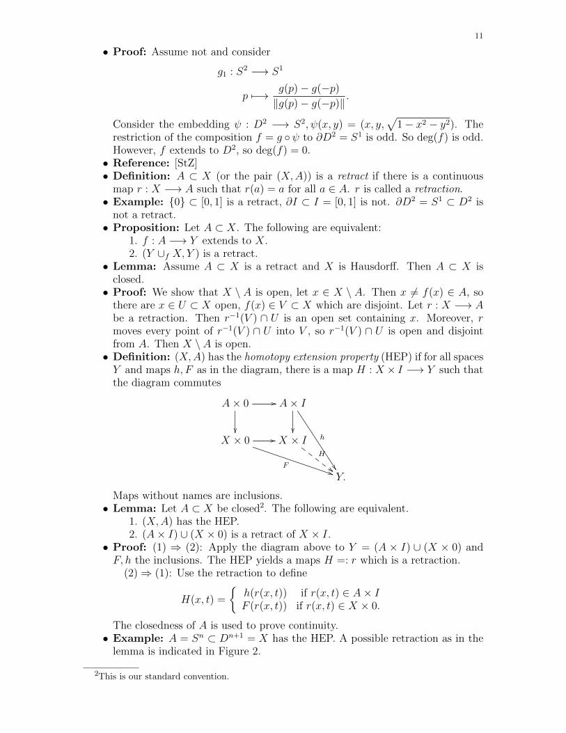
The closedness of A is used to prove continuity.• Example: A = Sn ⊂ Dn+1 = X has the HEP. A possible retraction as in the

lemma is indicated in Figure 2.

2This is our standard convention.

12

(x,t)

r(x,t)

t

x

Figure 2. Construction of a retraction Dn+1 × I −→ (Dn+1 × 0) ∪ (Sn × I)

• Example: X = I and A = {0} ∪ {n−1 |n = 1, 2, . . .} does not have the HEP.There is no retraction as in the above Lemma.

9. Lecture on Nov. 13 - Homotopy extension property, deformationretractions

• Definition: A continuous map f : X −→ Y is a homotopy equivalence if thereis a continuous map g : Y −→ X such that g ◦ f is homotopic to idX and f ◦ gis homotopic to idY . Then g is a homotopy inverse of f and X, Y are homotopyequivalent spaces.• Remark: Homotopy equivalence is an equivalence relation.• Examples:

– Homeomorphisms are homotopy equivalences.– Every convex (or star shaped) subset of Rn if homotopy equivalent to

one point.– S1 ↪→ R2 \ {(0, 0)} is a homotopy equivalence.– S1 is not homotopy equivalent to R2 (or any other contractible space):

Assume there is a homotopy equivalence f : S1 −→ R2 with g a homotopyinverse. Then since g◦f is homotopic to idS1 , so deg(g◦f) = 1. However,f , and hence g ◦ f is homotopic to a constant map. This implies deg(g ◦f) = 0.

• Definition: A space is contractible if it is homotopy equivalent to a point.• Theorem: Let (X,A) have the HEP and A contractible. Then the quotient

map X −→ X/A is a homotopy equivalence.• Proof: Fix a homotopy h : A× I −→ A with h(a, 0) = a and h(a, 1) = a0 for

all a and a suitable a0 ∈ A. Apply HEP to Y = X,F : X × 0 −→ X,F (x, 0) =x and h from above. We obtain a homotopy H : X × I −→ X such thatH(x, 0) = x, H(a, t) ∈ A and H(a, 1) = a0. Then

g : X/A −→ X

[x] 7−→ H(x, 1)

is well defined and a homotopy inverse of f , the required homotopies are pro-vided by H.• Definition: A ⊂ X is a deformation retract if there is a homotopy

H : X × I −→ X

such that H(·, 0) = idX , H(a, t) = a and H(x, 1) ∈ A for all x, a, t.• Examples:

– Sn × I ∪Dn+1 × 0 ⊂ Dn+1 × I is a deformation retract see Figure 2).– S1 ⊂ R2 \ {(0, 0)} is a deformation retract.

13

• Theorem: Let (X,A) be a CW-pair. Then X × 0 ∪ A × I is a deformationretract of X × I.• Proof: Xn+1×I∪X×0 is obtained from (Xn ∪ An+1)×I∪X×0 by attaching a

copies of Dn+1× [0, 1] ' Dn+2 along the subspace ∂Dn+1×I∪Dn+1×0 for eachn+1-cell in Xn+1 which is not in An+1. Since ∂Dn+1×I∪Dn+1×0 ⊂ Dn+1×Iis a deformation retract,( (

Xn ∪ An+1)× I ∪X × 0

)⊂ Xn+1 × I ∪X × {0}

is also a deformation retract. Let

hn+1 :(Xn+1 × I ∪X × {0}

)× J −→ Xn+1 × I ∪X × {0}

be the corresponding deformation retraction, such that

hn+1(x, 1) ∈(Xn ∪ An+1

)× I ∪X × 0,

so that hn+1 moves points (x, t) for x ∈ e when e is a n+ 1-cells of X which isnot in A. Then

hn+1((x, 0), s) = (x, 0) for all x ∈ Xhn+1((x, t), s) = (x, t) if (x, t) ∈ A× I.

Then the map H : (X × I)× J −→ X × I defined by

((x, t), s) 7−→

(x, t) if s = 0(x, t) if x ∈ Xn and s ≤ 2−(n+1)

hn ((x, t), 2n+1s− 1) if x ∈ Xn and 2−(n+1) ≤ s ≤ 2−n

hn−1 (hn((x, t), 1), 2ns− 1) if x ∈ Xn and 2−n ≤ s ≤ 2−(n−1) ≤ 1hn−2 (hn−1((x, t), 1), 2n−1 − 1) if x ∈ Xn and 2−(n−1) ≤ s ≤ 2−(n−2) ≤ 1

...

is continuous (even at s = 0). In order to see this note that H is the identity onthe k-skeleton for s close enough to 0. A map from X × I × J is continuous ifand only if it is continuous on the k-skeleton (X×I×J)k for all k. Therefore, His continuous. The homotopy H establishes that X×0∪A×I is a deformationretract of X × I.

Figure 3 is an attempt to illustrate what H is doing. The two thickened dotsat the bottom are elements of X0 \ A0 and the arrows indicate what happensto e × I for such a zero cell for s ∈ [1/2, 1]. Moreover, H((x, t), s) = (x, t) forx ∈ e ⊂ X0 and s ≤ 1/2.

The thickened horizontal line in X × 0 at the level s = 1/2 represents e× 0for a 1-cell e in X1 \ A1. The thickened, somewhat diagonal lines (one dashedone solid) represent e× I. The three arrows indicate how H (and h1 could acton points (x, t) for s ∈ [1/4, 1/2] when x ∈ e. For s ∈ [1/4, 1/2] points of theform (x0, t) with x0 ∈ X0 do not move.

• Corollary: CW-pairs (X,A) have the HEP.• Remark: It would have sufficed to show that X×0∪A× I is only a retract ofX × I, or, and this is not difficult, to show directly that (X,A) has the HEP:This can be done by induction over the skeleta using the fact that (Dn, Sn−1)has the homotopy extension property.

14

I

J

1/2

1

1/4

0-cells e of X 6⊂ A

1-cells e of X, e 6⊂ A

all e× I with e n-cell 6⊂ A for n ≥ 1

all e× I with e n-cell 6⊂ A for n ≥ 2

2-cells e of X, e 6⊂ A

0

x

e× I retracted to (e× 0) ∪ (e× I)

e× I retracted to (e× 0) ∪ (e× I)

never movepoints in X × 0 ∪ A× Ie× I retracted to e

pushed into X × 0 ∪ (A ∪X1)× I

pushed into X × 0 ∪ (A ∪X0)× I

Figure 3. What does H do?

• Warning: We did not show that (X × I,X × 0 ∪ A × I) is a CW-pair when(X,A) is a CW-pair.

In general, the product of two CW-complexes with the product topology isnot a CW-complex (the weak topology being finer than the product topology),see [Do] when the obvious cell decomposition and the obvious characteristicmaps are used. However, if one of the complexes is compact (i.e. finite), likeI, or only locally compact, then the product topology and the weak topologyon the product coincide.• For your information: A Hausdorff space is locally compact if every point

has a compact neighborhood (this implies that every neighborhood contains acompact neighborhood), and a CW complex is locally compact iff every pointhas a neighborhood that meets only finitely many closures of other cells.

The proof of these facts is not difficult but we omit them anyways (see [Sch],III.3.3. or [Do]).

15

10. Lecture on Nov. 16 - Homotopy equivalences

• Notation: I = [0, 1] and if there are intervals with different roles, I will try todenote one of them by I, the other one by J .• Theorem: Let A ⊂ X be a CW-pair and f, g : A −→ Y homotopic maps.

Then Y ∪f X and Y ∪g X are homotopy equivalent spaces.• Proof: Let H : A× I −→ Y be a homotopy. Then the space

Y ∪H (X × I)

contains Y ∪f X = Y ∪f (X × 0) and Y ∪g X = Y ∪g (X × 1) as subspaces.By the previous theorem X × 0∪A× I is a deformation retract of X × I. LetHdef : (X × I) × J −→ (X × I) be the corresponding homotopy relative toX × 0 ∪ A× I. The inclusion

ιf : Y ∪f X ↪→ Y ∪H (X × I)

has a homotopy inverse

Gf : Y ∪H (X × [0, 1]) −→ Y ∪f X = Y ∪H (X × 0 ∪ A× I)

[y] 7−→ [y]

[(x, t)] 7−→ [Hdef ((x, t), 1)]

Then Gf ◦ ιf = idY ∪fX and ιf ◦Gf is homotopic to the identity of Y ∪H (X× I)via Hdef . This homotopy is relative to Y .• Example: The last theorem together with the fact that X −→ X/A is a

homotopy equivalence when (X,A) has the HEP and A is contractible canbe used to produce interesting homotopy equivalences. For example, let K =T 2 ∪f D2 where f : ∂D2 −→ S1 × {0} ⊂ S1 × S1 = T 2 is a homeomorphism.Then K is homotopy equivalent to the 1-point union S1 ∨ S2.

11. Lecture on Nov. 20 - Cellular approximation theorem

• Definition: Let X, Y be CW-complexes and f : X −→ Y continuous. Thenf is cellular if f(Xn) ⊂ Y n for all n.• Warning: It is hard to overstate the importance of the following theorem!

Unfortunately, the proof is a bit more intricate than one might hope.• Theorem (Cellular approximation theorem): Every continuous map F :X −→ Y between CW-complexes is homotopic to a cellular map. The ho-motopy can be chosen relative to a subcomplex A of X where F is alreadycellular.• Remark: The analogous statement holds for maps of pairs F : (X,A) −→

(Y,B) . (Apply the cellular approximation theorem to A and use HEP of(X,A), then apply the relative version of the cellular approximation theoremto the remaining cells.)• Corollary: If f : Sn −→ Sm is continuous and m > n, then f is homotopic to

a constant map.• Proof of Corollary: Equip Sm with a CW-structure with cells of dimension

0 and m, and Sn with a CW-structure with cells of dimension ≤ n. Then-skeleton of Sm is then a point, so the corollary follows from the cellularapproximation theorem.

16

X X

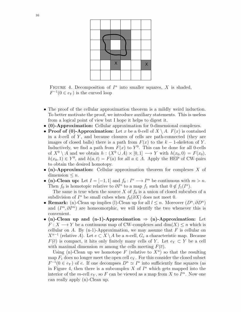
Figure 4. Decomposition of In into smaller squares, X is shaded,F−1(0 ∈ eY ) is the curved loop

• The proof of the cellular approximation theorem is a mildly weird induction.To better motivate the proof, we introduce auxiliary statements. This is uselessfrom a logical point of view but I hope it helps to digest it.• (0)-Approximation: Cellular approximation for 0-dimensional complexes.• Proof of (0)-Approximation: Let x be a 0-cell of X \A. F (x) is contained

in a k-cell of Y , and because closures of cells are path-connected (they areimages of closed balls) there is a path from F (x) to the k − 1-skeleton of Y .Inductively, we find a path from F (x) to Y 0. This can be done for all 0-cellsof X0 \ A and we obtain h : (X0 ∪ A) × [0, 1] −→ Y with h(x0, 0) = F (x0),h(x0, 1) ∈ Y 0, and h(a, t) = F (a) for all a ∈ A. Apply the HEP of CW-pairsto obtain the desired homotopy.• (n)-Approximation: Cellular approximation theorem for complexes X of

dimension ≤ n.• (n)-Clean up: Let I = [−1, 1] and f0 : In −→ Im be continuous with m > n.

Then f0 is homotopic relative to ∂In to a map f1 such that 0 6∈ f1(In).The same is true when the source X of f0 is a union of closed subcubes of a

subdivision of In be small cubes when f0(∂X) does not meet 0.• Remark: (n)-Clean up implies (l)-Clean up for all l ≤ n. Moreover (Dn, ∂Dn)

and (Im, ∂Im) are homeomorphic, we will identify the two whenever this isconvenient.• (n)-Clean up and (n-1)-Approximation ⇒ (n)-Approximation: LetF : X −→ Y be a continuous map of CW-complexes and dim(X) ≤ n which iscellular on A. By (n-1)-Approximation, we may assume that F is cellular onXn−1 (relative A). Let e ⊂ X \A be a n-cell, Ge a characteristic map. BecauseF (e) is compact, it hits only finitely many cells of Y . Let eY ⊂ Y be a cellwith maximal dimension m among the cells meeting F (e).

Using (n)-Clean up we homotope F (relative to Xn) so that the resultingmap F1 does no longer meet the open cell eY . For this consider the closed subsetF−1(0 ∈ eY ) of e. If one decompses Dn ' In into sufficiently fine squares (asin Figure 4, then there is a subcomplex X of In which gets mapped into theinterior of the m-cell eY , so F can be viewed as a map from X to Im. Now onecan really apply (n)-Clean up.

17

Let Yred be a subcomplex of dimension m+1 containing F (e)\eY and considerYred ∪λ eY where λ : ∂Dm −→ Yred is a gluing map for eY . By (n)-Clean up wemay assume that F (Ge(D

n)) does not meet 0 ∈ eY . Since eY is a deformationretract of eY \ 0 we can homotope F |e relative to X \ e (this is a CW-complex)so that the resulting map F1 does no longer meet eY .

After finitely many steps we have homotoped F relative to the complementof e so that the result maps e to Y n. This can be done for all n-cells of X atthe same time.• (n-1)-Approximation ⇒ (n)-Clean up: Notice that the Corollary above

for maps f : Sn−1 −→ Sl with l > n− 1 follows from (n-1)-Approximation.Let f : In −→ Im be continuous such that 0 6∈ f(∂In). Since f(∂In) is

closed there is a cube Q0 around 0 which is disjoint from f0(∂In). After areparametrization we may assume Q = [−1/3, 1/3]m. Let U = (−2/3, 2/3)m

and V = Im \ Q. This is an open cover of Im, so f−1(U), f−1(V ) is an opencover of In. Such a cover has a positive Lebesgue-number, so there is N suchthat the 1/N -cube neighborhood around each point of Im is contained in oneof the sets f−1(U), f−1(V ).

Let Xn = In be the regular CW-structure on In whose 0-skeleton con-sists of the points k1/N, . . . kn/N . Using (n-1)-Approximation (and the waythis is proved, namely using a deformation retraction of [−2/3, 2/3]m \ {0} to∂[−2/3, 2/3]m instead of a deformation retraction eY \ 0 to eY we may assumethat the n − 1-skeleton of X is mapped to V and the deformation does notaffect cells of X which were mapped entirely to V . The new map is called f ′.

Let k = (k1, . . . , kl) be the corner of a cell e of X (with∑ki minimal among

such corners) such that f ′(e) 6⊂ V . We arranged f ′(e) ⊂ VThen, by the first sentence of this proof, f ′(e) is homotopic to a constant

map inside of V since V is homotopy equivalent to Sm−1 and e is a n − 1-dimensional complex, and m > n by assumption. So there is an extensionf1 : e −→ V of the restriction of f ′ to e. Moreover, f1 and f ′ are homotopicrelative to e inside Im because Im is convex.• Proof of the cellular approximation theorem: This is a formality. Notice

(0)-Approximation relative A⇒ (1)-Clean up

⇒ (1)-Approximation relative A ∪X0 ⇒ (2)-Clean up

⇒ (2)-Approximation relative A ∪X1 . . .

The resulting homotopies hi : X × [0, 1] −→ Y relative to X i−1 ∪ A such thathi(·, 0) = hi−1(·, 1) (with h0(·, 0) = F , note X−1 = ∅) and h(X i, 1) ⊂ Y i cannow be assembled in a similar way as in the proof of the main theorem fromthe previous lecture:

H : X × [0, 1) −→ Y

(x, t) 7−→

h0(x, 2t− 2(20 − 1)) if t ∈ [0, 1/2]h1(x, 22t− 2(21 − 1)) if t ∈ [1/2, 3/4]h2(x, 23t− 2(22 − 1)) if t ∈ [3/4, 7/8]

...

hi(x, 2i+1t− 2(2i − 1)) if t ∈

[2i−1

2i, 2i+1−1

2i+1

].

...

18

If x ∈ Xn, then (x, t) is constant for t ≥ 2n+1−12n+1 . Thus we can extend H from

X × [0, 1) to X × [0, 1] by

H(x, 1) = hn(x, 1) for x ∈ Xn.

Because X has the weak topology with respect to cells/skeleta the extensionH is continuous everywhere. H(·, 1) is cellular.• Remark: To see an example of a surjective map I −→ I2 look at Exercise 12

of Chapter 5 in [Wa].• This concludes the discussion of general properties of CW-complexes. We now

look for tools to distinguish topological spaces up to homotopy equivalence.One such tool we applied already are sets of homotopy classes of maps S1 intoa space. When one adds a base point and considers homotopies relative to thebase point one obtains a much richer structure.

12. Lecture on Nov. 23 - Homotopy groups

• Definition: For x0 ∈ X, the pair (X, x0) a called a pointed space and x0 isthe basepoint. Continuous maps between pairs of spaces of this form are calledpointed.• Definition: Let x0 ∈ X. The fundamental group of (X, {x0}) is

π1(X, x0) = {γ : ([0, 1], {0, 1}) −→ (X, {x0}) continuous}/∼

where α ∼ β if these maps are homotopic as maps of pairs. If [α], [β] ∈π1(X, x0), we define

α ∗ β : ([0, 1], {0, 1}) −→ (X, {x0})

t 7−→{

α(2t) if t ∈ [0, 1/2]β(2t− 1) if t ∈ [1/2, 1].

(3)

This path depends on the choice of representatives, but the (relative) homotopyclass of the path α ∗ β is well defined.• Theorem: This defines a group structure on π1(X, {x0}).• Remark: If one replaces ([0, 1], {0, 1}) by (S1, z0) where z0 is any point of S1

all this can be reformulated. Often one uses z0 = 1 ∈ S1 ⊂ C.• Examples:

– If x0 is a deformation retract of X, then π1(X, x0) = {1} is trivial.– Let α, β : (S1, z0) −→ (S1, x0) be continuous. If these maps have different

degree viewed as maps S1 −→ S1, then they can’t be homotopic relativeto base points. If deg(α) = deg(β), then α ∼ β are homotopic relativeto basepoints. The proof of the second lemma on Nov. 6 produces ahomotopy relative to basepoints when the auxiliary path γ is chosenconstant. Moreover, in view of the definition (3) one can compute thedegree of α ∗ β since

ϕα∗β(t) =

{ϕα(2t) if t ∈ [0, 1/2]

deg(α) + ϕβ(2t− 1) if t ∈ [1/2, 1]

We obtain deg(α ∗ β) = ϕα∗β(1) = deg(α) + deg(β). Thus

deg : π1(X, x0) 7−→ Z[α] 7−→ deg(α)

is a group isomorphism.

19

– The loop α(t) = [cos(πt) : sin(πt) : 0], t ∈ [0, 1] represents an element ofπ1(RP2, [1 : 0 : 0]) such that α ∗ α is trivial in π1(RP2, [1 : 0 : 0]). It isnot obvious that α is non-trivial (but this is true).

• Definition: Let k ∈ {1, 2, . . .}. The k-th homotopy group πk(X, x0) of (X, x0)is

π1(X, x0) = {γ : (Ik, ∂Ik) −→ (X, {x0}) continuous}/∼ .

The product [α][β] = [α ∗ β] is by

α ∗ β : (Ik, ∂Ik) −→ (X, {x0})

(t1, . . . , tk) 7−→{

α(2t1, t2, . . . , tk) if t1 ∈ [0, 1/2]β(2t1 − 1, t2, . . . .tk) if t1 ∈ [1/2, 1].

(4)

• Theorem: This is determines a group structure on πk(X, x0).• Theorem: πk(S

n) = 0 for k < n (by cellular approximation).• Theorem: πk(X) is Abelian when k ≥ 2.• Remark: Since (Ik, ∂Ik) −→ (Sk, ∗) is a relative homeomorphism, one can

view maps (Ik, ∂Ik) −→ (Xk, ∗) as maps (Sk, ∗) −→ (X, ∗). This motivates• Definition: π0(X, x0) = {(S0, 1) −→ (X, x0)}/ ∼ where ∼ is again homotopy

relative to the base point. (Recall S0 = ∂D1 = {1,−1}.)• Remark: In general, π0(X, x0) does not have a group structure. It is a pointed

set since it has a distinguished element represented by S0 −→ {x0} ⊂ X. Bydefinition, elements of π0(X, x0) are in one-to-one correspondence with path-connected components of X.

13. Lecture on Nov. 27 - Role of the base point

• Theorem: πk(S1, 1) = {0} for all k ≥ 2.

• Proof: Let F : (Ik, ∂Ik) −→ (S1, 1) be continuous. This can be viewed a Ik−1

parametric family of maps fτ : (I, 0) −→ (S1, 1), τ ∈ Ik−1, for which we definedan auxiliary function ϕτ such that fτ (t1) = 1 · E(ϕτ (t1)). As shown on p. 9 inthe case k−1 = 1, these maps ϕτ can be assembled to a map Φ : Ik −→ R suchthat E(φ(t1, t2 . . . , tk)) = F (t1, . . . , tk) with τ = (t2, . . . , tk). If τ ∈ ∂Ik−1, thenfτ is constant and so is F |∂Ik . Hence φ|∂Ik ≡ 0 and one obtains a homotopyfrom F to the constant map by convex interpolation of φ and the vanishingmap (as in (2)).• Notation: It is common to omit the base point from πk(X, x0) or to write ∗

for some point.• Definition: Let [γ] ∈ π1(X, x0) and [A] ∈ πk(X, x0), k ≥ 1, then let

γ · A : (Ik × {1}) ∪ (∂Ik × J) −→ (X, x0)

(x, t) 7−→{A(x) if t = 1γ(t) if x ∈ ∂Ik.

There is a homeomorphism

ψ : (Ik, ∂Ik) = (Ik × {0}, ∂Ik × {0}) −→((Ik × {1}) ∪ (∂Ik × J), ∂Ik × {0}

)which is the identity/inclusion on ∂Ik × {0} (c.f. Figure 2). Then [(γ ·A) ◦ ψ]represents a well defined homotopy class [γ] · [A] in πk(X, x0).• Remark: For k = 1 this is the action of π1 on itself by conjugation.

20

• Theorem: The groups πi(X, x0) are π1(X, x0)-modules (more precisely, aZ[π1(X, x0)] module) with the module structure defined in the previous Defi-nition.• Remark: The module structure is independent from the choice of ψ (Alexander

trick, but beware of orientation reversing homeomorphisms...).• Remark: π1 is not Abelian in general, but there are more tools available to

compute this group than for πk, k ≥ 2. Even the groups πk(Sn) are not known.

A table with πk(Sn) for k ≤ 12 and n ≤ 8 can be found on p. 339 in [Ha].

• Remark: The choice of the base point matters. For example, if x0, x1 lie indifferent connected components of X, then there is no relationship betweenπk(X, x0) and πk(X, x1). If γ is path from x0 to x1, then

ϕγ : π1(X, x1) −→ π1(X, x0)

[α] 7−→ [γ ∗ α ∗ γ−1](5)

is a group homomorphism. Here γ−1(t) = γ(1−t) and ∗ denotes the concatena-tion of paths. The homomorphism depends on the homotopy class of γ relativeto the endpoints. If γ : [0, 1] −→ X is a path with γ(0) = x1, γ(1) = x0 weobtain a homomorphism ϕγ : π1(X, x0) −→ π1(X, x1) as in (5). Then

ϕγ ◦ ϕγ : π1(X, x1) −→ π1(X, x1)

α 7−→ (γ ∗ γ) ∗ α ∗ (γ ∗ γ)−1

is the conjugation of α with (γ ∗ γ) ∈ π1(X, x1), so ϕγ, ϕγ are isomorphisms.• Remark: α : (Sk, p) −→ (X, x0) represents the trivial element iff α extends to

a map Dk+1 −→ X. In this case it is called nullhomotopic.• Definition: α, β : (S1, 1) −→ (X, x0) are freely homotopic if they are homo-

topic but this homotopy does not have to respect base points. This notionmakes sense for homotopy classes.• Proposition: α, β ∈ π1(X, x0) are freely homotopic iff they are conjugate inπ1(X, x0).• Proof: If α, β : (S1, 1) −→ X are (freely) homotopic via H : S1× [0, 1] −→ X,

then let γ(t) = H(1, s). Then γ ∗ α ∗ γ−1 is homotopic to β since H providesan extension of γ ∗ α ∗ γ−1 ∗ β−1 : S1 −→ X to the disc (see Figure 5).

γ

γ

αβ

-1

Figure 5. γ ∗ α ∗ γ−1 ∗ β−1 is null homotopic

Conversely, we have to show that γ ∗α ∗γ−1 and α are freely homotopic. Weview γ∗α∗γ−1 as a map ([0, 1], {0, 1}) −→ (X, x0) with (γ ∗ α ∗ γ−1) (t) = γ(3t)for t ∈ [0, 1/3] and γ ∗α∗γ−1(t) = γ−1(3t−2) for t ∈ [2/3, 1]. Since we considerfree homotopies, the following homotopy is admissible (we identify [0, 1]/{0, 1}

21

with S1)

H : S1 × J −→ X

(t, s) 7−→{

γ ∗ α ∗ γ−1(t+ s/3) if t+ s/3 ≤ 1γ ∗ α ∗ γ−1(t+ s/3− 1) if t+ s/3 ≥ 1.

It shows that γ ∗ α ∗ γ−1 and α ∗ γ−1 ∗ γ are freely homotopic.• Using the Z[π1]-module structure one obtains a similar relationship betweenπk(X, x0) and πk(X, x1) for k ≥ 2. Note that a pointed map Sk −→ X whichfreely null homotopic is also null homotopic via pointed maps.• Theorem: Let (X, x0) be a CW-pair. Then πk(X, x0) depends only on thek + 1-skeleton of X.• Proof: Cellular approximation.• Definition: A pointed space is k-connected if πl(X, x0) is trivial for l ≤ k.

Instead of 0-connected one says path-connected, and instead of 1-connectedsimply connected.• Examples: CPn is simply connected for all n. The sphere Sk+1 is k-connected

for all k ≥ 0.• Definition: Let f : (X, x0) −→ (Y, y0) be a continuous map of pointed spaces.

The induced map on homotopy groups is

πk(f) : πk(X, x0) −→ πk(Y, y0)

[α] 7−→ [f ◦ α].

• Theorem: πk(f) is a well defined group homomorphism. It depends only onthe homotopy class of f as pointed map. Moreover, πk(g ◦ f) = πk(g) ◦ πk(f)if g : (Y, y0) −→ (Z, z0) is continuous.

14. Lecture on Nov. 30 – Induced maps, Seifert van Kampen

• Consequence: If f : X −→ Y is a homeomorphism of connected spacesand x0 a base point, then f∗ : πk(X, x0) −→ πk(Y, f(x0)) is an isomorphismwith inverse (f−1)∗. This is also obvious if f : (X, x0) −→ (Y, f(x0)) is ahomotopy equivalence relative to base points, the inverse is induced by thepointed homotopy inverse.• Notation: It is common to write πk(f), f#, f∗.• Example: fn : (S1, 1) −→ (S1, 1), z 7−→ zn induces the multiplication by n

on π1(S1, 1) ' Z. Recall that this isomorphism is given by the degree andnote that if deg(α) = ϕ(1) for a function ϕ as in (1), then ϕn, the functionassociated to fn ◦ α, is ϕn(·) = nϕ(·).• Theorem: Homotopy groups are homotopy invariants, i.e. homotopy equiva-

lent spaces have isomorphic homotopy groups.• Proof: Let X, Y be path connected. Assume that f : X −→ Y is a homotopy

equivalence with homotopy inverse g : Y −→ X. Then g ◦ f is homotopic tothe identity of X via H : X × [0, 1] −→ X with H(·, 0) = id. Let x0 ∈ X be abase point. Then choose y0 = f(x0), x1 = g(y0) and y1 = f(x1). Then

f∗ : πk(X, x0) −→ πk(Y, y0) g∗ : πk(Y, y0) −→ πk(X, x1)

are well defined. Let γ : [0, 1] −→ X, γ(t) = H(x0, 1 − t). This is a path fromx1 to x0. Then g ◦ f ◦α is homotopic to γ ·α for all α representing elements of

22

πk(X, x0). In particular, g∗ is surjective and f∗ is injective. Now consider

f∗∗ : πk(X, x1) −→ πk(Y, y1)

and apply the same argument to f ◦ g : (Y, y0) −→ (Y, y1) to show that f∗∗ ◦ g∗is an isomorphism. Hence g∗ : πk(Y, y0) −→ πk(X, x1) is an isomorphism.• Remark: If one considers pointed homotopy types (i.e. pointed, path con-

nected spaces up to pointed homotopy equivalence), then one obtains muchneater proofs and nicer statements because the pointed homotopy inverse g tothe pointed homotopy equivalence f induces the inverse to f∗.• Theorem: The map

πk(X, x0)× πk(Y, y0) −→ (X × Y, (x0, y0))

([α], [β]) 7−→ [(α(·), β(·))](6)

is an isomorphism.• Proof: This map is injective: If (α, β) : (Ik, ∂Ik) −→ (X × Y, ∗) is nullhomo-

topic, then the composition

prX ◦ (α, β) : (Ik, ∂Ik) −→ (X × Y, (x0, y0)) −→ (X, x0)

x 7−→ (α(x), β(x)) 7−→ α(x)

is nullhomotopic (with the projection prX : (X × Y, (x0, y0)) −→ (X, x0)).Similarly for β and Y .

This map is surjective: If γ : (Ik, ∂Ik) −→ (X × Y, (x0, y0)) represents ahomotopy class, then γ = (prX ◦ γ, prY ◦ γ).

This map is a group homomorphism: Direct check.• Remark: The following theorem is the result of the application of the Seifert-

van Kampen Theorem to CW-complexes. Depending on how we progress, wemight prove this Theorem (and the following consequence), or not.• Set up: Let (X, x0) be a connected CW-complex with x0 ∈ X0 and Γ0 a

maximal tree in X1 with x0 ∈ Γ. Orient all 1-cells which are not in Γ and letγi, i ∈ I, be the collection of 1-cells which are not contained in Γ and considerthe free group FI which is generated by γi, i ∈ I.• For your information: Let S be a set. The free group FS generated byS comes with an inclusion ι : S ↪→ FS and satisfies the following universalproperty:

For all groups G and maps f : S −→ G of sets there is a unique grouphomomorphism ϕ such that ϕ ◦ ι = f .

FS

ϕ

��S

ι>>

f// G

• Theorem, part 1: π1(X1, x0) ' FI .• Example: The fundamental group of the figure 8 (this is a one-point union of

two circles) is isomorphic to Z ∗ Z, i.e. the free group on two generators.• Set up: We write i : (X1, x0) −→ (X, x0) for the inclusion map. For each 2-celle of X choose a characteristic map Fe : D2 −→ X2. Fix a base point e0 in ∂D2.After a homotopy of Fe we may assume Fe : (S1 = ∂D2, e0) −→ (X1, x0). Then

23

let N be the smallest normal subgroup containing all elements of the form

(7) (Fe)∗

id : S1 −→ D2︸ ︷︷ ︸generator of π1(∂D2,e0)

∈ π1(X1, x0).

• Theorem, part 2: The map i∗ : π1(X1, x0) −→ π1(X, x0) is surjective andhas kernel N . Hence π1(X, x0) ' π1(X1, x0)/N .• Remark:

1. surjective follows from cellular approximation, it is equally clear thatN ⊂ ker(i). The most difficult step is to show that ker(i) ⊂ N . For aproof see [Ha], p. 43–54 or [StZ], Section 5.3.

2. We homotope Fe to arrange that Fe(e0) = x0. In general, there are manyways to do that, so the element of π1(X1, x0) described in (7) is welldefined only up to conjugation (by the base point discussion last time).Since N is the smallest normal subgroup containing these elements, thisambiguity does not matter.

• Example: RP2 has a CW-structure X with exactly one cell in dimension

0, 1, 2 such that X1 ' S1 and RP2 = X2 = X1∪f D2

where the map f : ∂D2

=S1 −→ S1 has degree ±2. Hence π1(X1, x0) = Z. Since f has degree ±2, theimage of π1(∂D2, ∗) in π1(X1, x0) ' Z consists of maps of even degree. Henceπ1(RP2, x0) ' Z/2Z. Because RPn, n ≥ 2, has a CW-structure such that the2-skeleton is RP2, it follows that

π1(RPn, ∗) = Z/2Z for n ≥ 2.

• Application (Sketch): Let G be a group. There is a pointed CW-complex(X, x0) such that π1(X, x0) ' G. To construct X, consider X0 = {x0}. Foreach element g ∈ G attach a 1-cell γg to X0, oriented in a way. Then for allg, h ∈ G consider the path γg ∗ γh ∗ γ−1

gh in X1 and attach a 2-disc to X1 alongthis path. There is a well defined group homomorphism

ψ : G −→ π1(X, x0)

g 7−→ γg.

To find an inverse consider [γ] ∈ π1(X). After a homotopy, we may assumethat γ is cellular and the way γ travels through X1 determines a finite wordγg1 ∗ γg2 ∗ . . . γgk . Then

π1(X, x0) −→ G

[γ] 7−→ g1 · g2 · . . . gk.

This is a well defined inverse of ψ.

15. Lecture on Dec. 4 – Coverings, Path lifting

• Reference: Chapter 9 in [Ja], Chapter 6 in [StZ],• Definition: Let pr : Y −→ X be continuous. This map is a covering (map)

if for all x ∈ X there is an open neighborhood U ⊂ X, a discrete topological

24

space Λ, and a homeomorphism ϕ : pr−1(U) −→ U × Λ such that

(8) pr−1(U)ϕ //

pr##

U × Λ

pr1||U

commutes. Here pr1 is the projection on the first factor. A neighborhoodU with this property is called trivializing. When using such neighborhoods weimplicitly fix Λ and ϕ as above.• Remark: If pr is a covering, and x ∈ X, then the fiber Yx := pr−1(x) =ϕ−1

({x} × Λ

)is discrete and homeomorphic to Λ. The function x −→ |Yx| is

locally constant, and constant if X is connected. If this function is constantand finite, then pr is said to be n-sheeted with n = |Y (x)|. If it is constant andinfinite, then it has infinitely many sheets.• Examples:

– id : X −→ X is a covering, it is 1-sheeted.– E : R −→ S1, E(x) = e2πit is a covering. It has infinitely many sheets.

Same for exp : C −→ C \ {0}.– For n ∈ {1, 2, . . .}, the map fn : S1 ⊂ C −→ S1, z 7−→ zn is a covering

and n-sheeted. Same when fn is viewed as map C \ {0} −→ C \ {0}.– The quotient map Sn −→ RPn is a covering, it is 2-sheeted. For [x] ∈RP2,

Λ[x] =

{x

‖x‖,− x

‖x‖

}.

For x ∈ RP2 let U = {[y] | 〈y, x〉 6= 0}. Then

pr−1(U) = {y ∈ S2 | 〈y, x〉 6= 0}= {y ∈ S2 | 〈y, x〉 > 0}︸ ︷︷ ︸

U+

∪{y ∈ S2 | 〈y, x〉 < 0}︸ ︷︷ ︸U−

where the union is disjoint. Moreover, pr : U± −→ U is a homeomor-phism. Then

u ∈ U+� // ([u],+1)

u ∈ U− � // ([u],−1)

pr−1(U)

pr&&

U+ ∪ U− ϕ// U × {±1}

pr1ww

U

– If Λ 6= ∅ is discrete, then pr : X × Λ −→ X is a covering.– The inclusion (−∞, 0) −→ R is not a covering although there is a dia-

gram like (8) for all points in the image.– The groups Spin(n) which appear in the definition of Spin-structures

and Dirac operators are 2-sheeted coverings of SO(n), for the definitionof Spin(n) see [BrtD] p. 54–63.

25

• Definition: Two coverings pr0 : Y0 −→ X and pr1 : Y1 −→ X are isomorphicif there is a homeomorphism ϕ : Y0 −→ Y1 such that

(9) Y0ϕ //

pr0

Y1

pr1��X

commutes. The definition is analogous for pointed coverings.• Definition: Let f : Y −→ X be continuous. f is a local homeomorphism if

every y ∈ Y has a neighborhood U such that f |U is a homeomorphism onto itsimage and f(U) is a neighborhood of f(y).• Fact: Coverings are local homeomorphisms, so is the inclusion in the list above.E|(0,2) : (0, 2) −→ S1 is a surjective local homeomorphism, albeit not a covering.• Fact: Local homeomporphism are open, i.e. they map open sets to open sets.

Let f : Y −→ X be a local homeomorphism and U ⊂ Y open. For each y ∈ Ylet Uy be an open neighborhood in U of y as above. Then

f(U) =⋃y∈Y

f(U ∩ Uy︸ ︷︷ ︸open in X

)

is a union of open sets in X.• Consequence: 1-sheeted coverings are homeomorphisms.• Warning: Local homeomorphisms are not closed, in general. Neither are

covering maps. However, this is the case when X is Hausdorff and Y is compact.• Fact: If f : Y −→ X is a finite sheeted covering of a compact space X, thenY is compact.• The following notion is fundamental in the study of covering spaces.• Definition: Let f : Y −→ X be continuous, f(y0) = x0 and α : [a, b] −→ X

a path. A path α : [a, b] −→ Y with starting point y0 is a lift of α withinitial point y0 if f ◦ α = α. A map f has the path lifting property if for everyα : [0, 1] −→ X and y0 with f(y0) = α(0) = x0 there is a unique lift α withinitial point y0.• Example: Look at the first Lemma in the lecture on Nov. 6.• Lemma: Covering maps have the path lifting property.• Proof: Let pr : Y −→ X be a covering and

T :=

{t ∈ [0, 1]

∣∣∣∣ there is a unique α : [0, t] −→ Y such thatα(0) = y0 and pr(α(s)) = α(s) for s ∈ [0, t]

}.

This set contains 0. Let τ = supT . If τ = 1 we are done. If not, let αbe the unique lift of α|[0,τ), fix a trivializing neighborhood U of α(τ) and ahomeomorphism ϕ : pr−1(U) −→ U × Λα(τ). We denote ϕ(α(τ)) = (α(τ), λ0).Then for ε > 0 small enough, α((τ − ε, τ + ε)) ⊂ U and

α : [0, τ + ε) −→ Y

t 7−→{

α(t) if t < τϕ−1(α(t), λ0) if t ≥ τ − ε

is continuous and a lift of α with starting point y0. This lift is unique on[0, τ) by assumption and on (τ − ε, τ + ε) a lift is uniquely determined byλ0 = pr2(ϕ(α(τ−ε/2)) and α|(τ−ε,τ+ε) because Λ is discrete. Hence τ+ε/2 ∈ Tcontradicting to the choice of τ . Hence τ = 1 and T = [0, 1].

26

16. Lecture on Dec. 7 – Homotopy lifting, characteristic subgroups

• Remark: The following Lemma is a parametric version of the previous one.• Lemma (Homotopy lifting for coverings): Let pr : Y −→ X be a covering,

h : Z × [0, 1] −→ X a homotopy and h0 : Z = Z × {0} −→ Y a lift of h(·, 0),

i.e. pr(h0(z)) = h(z) for all z ∈ Z.

Then there exists a unique continuous map h : Z × [0, 1] −→ Y such that

pr(h(z, t)) = h(z, t) and h0(z) = h(z, 0):

Z × {0} h0 //

��

Y

pr

��Z × I h //

h

::

X.

• Proof: Uniqueness follows for the previous lemma since the restriction of a

lift h to {z} × [0, 1] is a lift of the path h|{z}× I with initial point h0(z). This

also means that we can define h as a family of path lifts with initial point

determined by h0. We call the result h but we still have to show that this iscontinuous. Let z ∈ Z. We consider

T :=

t ∈ [0, 1]

∣∣∣∣∣∣there is a neighborhood V of z ∈ Z and ε > 0 such that

h(V × (t− ε, t+ ε)) is contained in ϕ−1(U × {λ})for a trivializing neighborhood U of h(z, t) and λ ∈ Λ

.

If t ∈ T , then h|V is continuous on a neighborhood of (z, t). Now T is open by

definition, T contains 0 since h0 and h are continuous. Let t0 ∈ T . Then thereis a trivializing neighborhood U of h(z, t0), ε > 0, and V a neighborhood of zsuch that h(V × (t − ε, t + ε)) ⊂ U . Since t0 ∈ T there is t1 with t1 ∈ T and

|t1−t0| < ε. Then there is a neighborhood V1 of z in Z such that h((V1×{t1}) ⊂ϕ−1(U × {λ}). But then h(z′, t) ⊂ ϕ−1(U × {λ}) for t ∈ (t0 − ε, t0 + ε) andz′ ∈ V1 since Λ is discrete. Hence t0 ∈ T and T = [0, 1] since [0, 1] is connected.• Consequence: The map pr∗ : π1(Y, y0) −→ π1(X, x0) is injective.• Consequence: The map pr∗ : πk(Y, y0) −→ πk(X, x0) is an isomorphism• Definition: A space X is locally path connected if for all x ∈ X every neigh-

bourhood V of x contains a path connected neighbourhood V ′ of x.• Examples:

– CW-complexes are locally path connected.– For M = {0} ∪ {1, 1/2, 1/3, 1/4, . . .} consider the cone CM = (M ×I)/(M ×{1}) of M . Then CM is path connected (even contractible) butnot locally path connected.

• Theorem: Let Y be locally path connected and path connected. Let pr :

X −→ X be a covering and f : Y −→ X a continuous map. Fix y0 ∈ Y ,

x0 ∈ X and x0 ∈ X such that f(y0) = x0 = pr(x0). Then the following areequivalent:

1. There is a unique map f : (Y, y0) −→ (X, x0) such that pr ◦ f = f .

2. f∗(π1(Y, y0)) ⊂ pr∗(π1(X, x0))

27

X

pr

��Y

f//

f??

X

• Proof: (1)⇒(2): Assume that the lift f exists. Then

f∗(π1(Y, y0)) = pr∗

(f∗(π1(Y, y0))

)⊂ pr∗(π1(X, x0)).

(2)⇒(1): Let y ∈ Y and fix a path γy : [0, 1] −→ Y such that γy(0) = y0 andγy(1) = y. We define

f(y) = end point of the lift of f ◦ γy to X with starting point x0.

This is well defined: Let γ′y be another path in Y from y0 to y. By assumption,

there is [α] ∈ π1(X, x0) such that pr ◦ α is homotopic to f ◦(γy ∗ γ′−1

y

)relative

to x0. By the homotopy lifting lemma, [α] has a representative, we call it α′,which is a lift of f ◦

(γy ∗ γ′−1

y

). Since all homotopies are relative to basepoints,

pr−1(x0) is discrete, and α is a closed loop, the same is true for α′. Hence thelifts of f ◦ γy and f ◦ γ′y have the same endpoints. Thus we have a well defined

map f : Y −→ X such that pr ◦ f = f .

f is continuous: Let x ∈ X and pr(x) = x and assume that x = f(y). Then

there is a path γy from y0 to y such that the lift of f ◦ γy to X with startingpoint x0 ends at x. Let U ⊂ X a trivializing open neighborhood of x. There isλ ∈ Λ such that pr−1(U) ' U × Λ and ϕ−1(U × {λ}) is an open neighborhood

of x = (x, λ). Let W ⊂ U ×{λ} be neighborhood of x. Then f−1(pr(ϕ−1(W )))contains a path connected neighbourhood V of y

Every point v ∈ V can be reached from y0 by a path of the form γy ∗ σvwhere σv is a path in V from y to v. Lifts of f ◦ (γy ∗σv) end in ϕ−1(W ). Since

W can be chosen arbitrarily small, this implies that f is continuous.Uniqueness: follows from the uniqueness for the lift of paths.

• Definition: Let pr : (Y, y0) −→ (X, x0) be a path connected covering whichpreserves base points. The characteristic subgroup of pr is C(Y, y0) = pr∗(π1(Y, y0)).• Lemma: [γ] ∈ pr∗(π1(Y, y0)) iff the lift of γ to Y with starting point y0 is

closed (i.e. the endpoint of the lift is also y0).• Proof: Let [γ] ∈ π1(Y, y0) be a loop, then pr ◦ γ has a closed lift (namely γ)

and by homotopy lifting the same is true for all closed loops based at x0 whichare homotopic to pr ◦ γ (homotopy relative to x0).

The converse is obvious: Let γ ∈ π1(X, x0) such that the lift γ to Y withstarting point y0 is closed. Then pr∗([γ]) = [γ].• Corollary: Let (Y0, y0) and (Y1, y1) be two coverings of (X, x) such thatC(Y0, y0) = C(Y1, y1). Then the coverings are isomorphic as pointed cover-ing spaces.

28

• Proof: Let ϕ0 be the lift of pr0 and ϕ1 be the lift of pr1. The following diagramcommutes since lifts are unique, hence ϕ1 ◦ ϕ0 = id : Y0 −→ Y0.

(Y0, y0) ϕ0

//

pr0 %%

id++

(Y1, y1)

pr1��

ϕ1

// (Y0, y0)

pr0yy(X, x).

• Observation: Assume that pr : Y −→ X is a path connected covering andy0, y

′0 ∈ pr−1(x0). Then the characteristic subgroups of

pr : (Y, y0) −→ (X, x0) pr′ : (Y, y′0) −→ (X, x0)

are conjugate: Let γ be a path in Y from y0 to y′0. Then pr ◦ γ is a closed loopbased in x0. Since conjugation with γ induces isomorphisms of fundamentalgroups, there is a loop α′ based at y′0 such that γ ∗ α′ ∗ γ−1 is homotopic to α.Then pr ◦ α = pr(γ ∗ α′ ∗ γ−1) = (pr ◦ γ) ∗ (pr′ ◦ α′) ∗ (pr ◦ γ−1). Hence.

pr∗(π1(Y, y0)) = [pr ◦ γ] · pr′∗ (π1(Y, y′0)) · [pr ◦ γ]−1 .

• Consequence: If pr : Y −→ X is a path connected covering, then the con-jugacy class of the characteristic subgroup of π1(X, x0) is independent of thechoice of base point in Y .

• Theorem: Let pr : (X, x0) −→ (X, x0) a locally path connected and pathconnected covering and f : (Y, y0) −→ (X, x0) continuous. The following areequivalent:

1. There is a lift f : Y −→ X of f , i.e. pr ◦ f = f .2. f∗(π1(Y, y0)) is conjugate to a subgroup of the characteristic subgroup of

pr : (X, x0) −→ (X, x0).

• Proof: (1)⇒(2): Let f be a lift and x′0 = f(y0). We write pr′ : (X, x′0) −→π1(X, x0). Let γ is a path in X from x0 to x′0 = f(y0). Then

f∗(π1(Y, y0)) = (pr′ ◦ f)∗(π1(Y, y0))

⊂ pr′∗

(π1(X, x′0)

)= [pr ◦ γ]−1 · pr∗

(π1(X, x0)

)· [pr ◦ γ].

(2)⇒(1): Assume that f∗(π1(Y, y0)) ⊂ [β] · pr∗(π1(X, x0)) · [β]−1 for β ∈π1(X, x0). Let β−1 be a lift of β−1 to X with initial point x0. Then

f∗(π1(Y, y0)) ⊂ [β] · pr∗(π1(X, x0)) · [β]−1

= [pr ◦ β] · pr∗(π1(X, x0)) · [pr ◦ β]−1

= pr∗

(β ∗ π1(X, x0) ∗ β−1

)= pr∗

(π1(X, β(0))

)According to the Lifting lemma from above there is a (unique) lift f : (Y, y0) −→(X, β(0)

)of f to X which maps y0 to β(0).

29

• Corollary: Let Y0 and Y1 be two covering spaces of X (both path connectedand locally path connected). Then Y0, Y1 are isomorphic iff the characteristicsubgroups are conjugate.• Reminder: The index of a subgroup H ⊂ G is the cardinality of G/H, this

equals the cardinality of H\G.• Remark: Let pr : (Y, y0) −→ (X, x0) be a path connected covering, Y path

connected, and Λ0 = pr−1(x0). For each yi ∈ Λ pick a path γi, yi ∈ Λ in Y fromy0 to yi. Then for every path α representing an element of C(Y, yo) · [pr ◦ γi]the lift α to Y with initial point y0 ends in yi. This establishes a bijective map

C(Y, y0)∖π1(X, x0)︸ ︷︷ ︸

right cosets

−→ Λ0.

• Corollary: If pr : Y −→ X is a n-sheeted covering, then C(Y, y0) has index nin π1(X, x0) (for all y0 ∈ pr−1(x0)).• Definition: Let X be a space and G a group. A (left) group action of G onX is a homomorphism ρ : G −→ Homeo(X) such that ρ(gh) = ρ(g) ◦ ρ(h). Aright group action satisfies ρ(gh) = ρ(h) ◦ ρ(g).• Definition: Let pr : Y −→ X be a covering. A decktransformation is a

homeomorphism f : Y −→ Y such that pr ◦ f = pr. They form the groupDeck(pr) of decktransformations and acts on Y from the left.• Remark: Let pr : Y −→ X be a path connected and locally path connected

covering and f, g two decktransformations. If f(y0) = g(y0) for some y0 ∈ Y ,then f ≡ g by unique lifting.• Examples:

– pr = E : R −→ S1, E(t) = e2πit. Then fn : R −→ R, fn(t) = t + n is adecktransformation for n ∈ Z. The deckgroup is Z.

– prn : S1 −→ S1, prn(z) = zn. Let ζ be a n-th root of unity. Thenfm : S1 −→ S1, fn(z) = ζmz is a decktransformation for n ∈ Z. Thedeckgroup is Zn.

– pr : S2 −→ RP2. Then f = −id is a decktransformation, the deckgroupis Z2.

• Definition: Let G be a group and H a subgroup. The normaliser of h in G isthe largest subgroup N(H) ⊃ H such that H is normal in H.• Remark: The normaliser is well defined since any two subgroups of G in whichH is normal generate a subgroup of G with the same property.• Warning: There is notation clash here: I will frequently write H\N(H) for

the quotient group (represented by right cosets, which coincide with left cosetssince H is normal in N(H)). This is to be distinguished from the complementH \ N(H) of N(H) in H by the reader (the latter possibility would alwaysdenote the empty set).• Theorem: Let pr : (Y, y0) −→ (X, x0) be a path connected and locally path

connected covering with base points and C = C(Y, y0) = pr∗(π1(Y, y0)) itscharacteristic subgroup. Then

Γ : C∖N(C) −→ Deck(pr)

[γ] 7−→ lift of pr to (Y, γ(1)) where γ is a lift ofγ to Y with initial point y0

(10)

30

and

Deck(pr) −→ C∖N(C)

f 7−→ [pr ◦ γ] where γ is a path in Y from y0 to f(y0)

are mutually inverse homomorphisms.• Remark: Deck(pr) is defined without reference to a base point. For g ∈ π1(X),

the groups C\N(C) and (gCg−1)\N(gCg−1) are canonically isomorphic.• Proof: well defined maps: first consider Γ : N(C) −→ Deck(pr). Let γ ∈N(C(Y, y0)) ⊂ π1(X, x0) and γ the lift of γ to Y with initial point y0. Then

C(Y, γ(1)) = [pr ◦ γ]−1 · C(Y, y0) · [pr ◦ γ]

= [γ]−1C(Y, y0)[γ] = C(Y, y0)

because γ lies in the normaliser of C(Y, y0). According to the lifting theoremabove, there is a unique lift

(Y, γ(1))

pr

��(Y, y0) pr

//

Γ(γ)99

(X, x0)

This map is well defined on right cosets since lifts of loops in C(Y, y0) are closed.Thus Γ as in (10) is well defined. and we have also showed that Γ is injective

Let f ∈ Deck(pr) and γ a path from y0 to f(y0). Then, since pr ◦ f = pr,f can be viewed as a lift of pr to a map f : (Y, y0) −→ (Y, f(y0)). Hencepr∗(π1(Y, y0)) = C(Y, y0) ⊂ C(Y, f(1)). The same argument applied to f−1

shows C(Y, f(1)) ⊂ C(Y, y0).Now let γ be a path from y0 to f(1). Then π1(Y, f(1)) = [pr◦γ]−1π1(Y, y0)[pr◦

γ]. Projecting this to (X, x0) we obtain C(Y, f(1)) = [γ]−1 · C(Y, y0) · [γ] =C(Y, y0). Therefore γ ∈ N(C). This shows that the second map is well defined.

Γ is a group homomorphism: Let α, β ∈ N(C) and α, respectively β, be the

lift of α respectively β, with initial point y0 and β be the lift of β with initialpoint α(1). Now Γ(α) is a deck transformation which moves y0 to α(1), so

Γ(α) ◦ β = β. Therefore

Γ(α · β)(y0) = α ∗ β(1) = α ∗ β(1) = β(1)

= Γ(α)(β(1)

)= Γ(α)

(Γ(β)(y0)

).

Group homomorphism, second map: Let f, g be two decktransformations, α

a path from y0 to f(y0) and β a path from y0 to g(y0). Then α ∗ (f ◦ β) is apath from y0 to (f ◦ g)(y0). Because f is a deck transformation[

pr ◦(α ∗ (f ◦ β)

)]= [pr ◦ α] · [pr ◦ f ◦ β]

= [pr ◦ α] · [pr ◦ β].

This shows that that the second map is a group homomorphism.The maps are mutally inverse: This can be read of from the definitions.

• Consequence: C\N(C) acts on Y from the left.

31

• Definition: A path connected covering Y −→ X is called universal if the char-acteristic subgroup is {1}. It is regular or normal if its characteristic subgroupis normal in π1(X).• Corollary: If pr : Y −→ X is a normal covering, then Deck(pr) acts transi-

tively on fibers, i.e. for all x0 and y0, y′0 ∈ pr−1(x0) there is f ∈ Deck(pr) such

that f(y0) = y′0.• So far we have studied coverings and their isomorphisms/automorphisms. In

particular, there is at most one (up to isomorphism) covering of X (path con-nected, locally path connected space) whose characteristic subgroup is conju-gate to a given subgroup C ⊂ π1(X). We want to study under which conditionssuch a covering exists. This needs some vocabulary.• Definition: Let G be a group. A G-action on a space X is properly discontin-

uous if for all x ∈ X there is an open neighborhood U such that gU ∩ U = ∅for all g 6= 1. The same for right G-actions.• Remark: If G y X is properly discontinuous, then g · x = x implies g = 1,

i.e. properly discontinuous actions are free.• Warning: There is another property of G y X which is also called properly

discontinous: X has to be locally compact and for all compact K ⊂ X the set{g |K ∩ gK 6= ∅} is finite.• Example: The deck group action on a covering is properly discontinuous (look

at preimages of trivializing neighbourhoods)• Example: Let Z y S1 be defined by n · z = e2πinaz for a ∈ R \Q. This group

action is free, but not properly discontinuous.

• Theorem: Let pr : (X, x0) −→ (X, x0) be the universal covering of the pathconnected and locally path connected space X and H ⊂ π1(X, x0) a subgroup.Then X has a covering with characteristic subgroup H.

• Proof: Consider the homomorphism Γ and Γ(H) ⊂ Deck(X, x0) from (10) andlet

prH : (X, x0) = (Γ(H)\X, [x0]) −→ (X, x0)

[y] 7−→ pr(y).

Let [y] ∈ X and U an open neighbourhood of y such that U ∩ g · U = ∅ forg 6= 1. Then g ·U, g ∈ G, is a pairwise disjoint collection of open sets such that∪g(g ·U) = pr−1(pr(U)). In particular, pr(U) ⊂ X is open, pr|U : U −→ pr(U)is a homeomorphism, and

(pr|U(u),Γ(h)) � // Γ(h)(u)

pr|U(U)× Γ(H) ϕ//

pr1 ''

pr−1(pr(U))

prxxpr(U)

establishes that prH is a covering.

Let [α] ∈ π1(X, x0) and consider the lift α of α to X with initial point x0.This is closed if and only if the lift of α has endpoint in Γ(H), i.e. [α] ∈ H.• Consequence: Let (X, x0) be connected, locally path connected space with

base point x0 and H ⊂ π1(X, x0) a subgroup. In order to show that there is

32

a covering with characteristic group H it is enough to construct the universalcover.• Definition: A topological space X is semi locally simply connected if for everyx ∈ X and every neighborhood U of x there is a neighbouhood U ′ ⊂ U suchthat every loop in U ′ is null homotopic in X.• Example: cone over the Hawaiian earrings.• Terminology: A space is sufficiently connected if it is path connected, locally

path connected, and semi locally simply connected.• Theorem: Let X be a sufficiently connected space. Then there is there is a

universal covering pr : Y −→ X.• Proof Idea/Stroke of genius: We need a space with the path lifting property.

Let γ : ([0, 1], 0) −→ (X, x0) be a path in X. Then

[0, 1] −→ P(X, x0) = {Paths γ : [0, 1] −→ X starting at x0}

s 7−→(γs : [0, 1] −→ X

t 7−→ γ(st)

)(11)

is a lift of γ to the set P(X, x0) with respect to the end point map

pr : (P(X, x0), c0) −→ (X, x0)

γ 7−→ γ(1)

where c0 is the constant path sitting at x0. This only a set theoretic cover, and ifγ is homotopic of γ′ are homotopic relative there end points, then the endpoints(namely the paths γ and γ′) are not equal. This suggests we should look atspaces of paths with the equivalence relation homotopy relative endpoints. Itturns out that this can be carried out.• Proof: We consider

X = { paths in X starting in x0}/ ∼

with ∼ being homotopy relative to the endpoints. As base point in X we takethe (homotopy class of) the constant path c0(t) ≡ x0. The projection is

pr : (X, c0) −→ (X, x0)

[γ] 7−→ γ(1).

This is well defined since we use homotopy relative to end points as equivalence

relation. We need to define a topology on X with all kinds of properties.

Let γ ∈ X and U a path connected neighbourhood of γ(1). Then let

V (γ, U) = (γ ∗ {paths in V startign in γ(1)})/

homotopy relative endpoints.

Definition of the topology on X: A set V ⊂ X is open if and only of forevery point [γ] in V there is γ ∈ [γ] and γ(1) ⊂ U ⊂ X such that V (γ, U) ⊂ V .

Topology: direct checkpr is continuous: Let U ⊂ X open and [γ] ∈ pr−1(U). Because U is

open and X is locally pah connected, there is U ′ ⊂ U around γ(1). ThenV (γ, U ′) ⊂ U . This shows that pr is continuous.

X is path connected: Let γ represent [γ]. Then s 7−→ γs is a path (asin (11)) starting at c0 and ending at γ once we show it is continuous. Lets0 ∈ [0, 1]. There is a path connected neighborhood U of γs(1) = γ(s) andbecause γ is continuous it spends some time in U , i.e. there is ε > 0 such thatγ((s0 − ε, s0 + ε)) ⊂ U . Then γs ∈ V (γs0 , U) for s ∈ (s0 − ε, s0 + ε).

33

pr has discrete fibers: Let x ∈ X and γ a path from x0 to x (representing

a point in X). Because X is semi locally simply connected, there is a pathconnected U ⊂ X such that i∗ : π1(U, x) −→ π1(X, x) is trivial. Then V (γ, U)is open and contains no other point of pr−1(x).

pr is locally trivial: very similar to the last step.

X is simply connected: Let γs : [0, 1] −→ X be a loop of paths such that

s 7−→ [γs] is continuous (in the topology on X, not necessarily in any othernatural topology on the space of paths). Then σ : tau 7−→ γτ (1) is a path suchthat s 7−→ σ(s·) is homotopic (relative endpoints) to γs. Since [γ1] is homotopicrelative endpoints to the constant path. The resulting homotopy can used toshow that the original loop of paths is null-homotopic.

17. Lecture on Jan. 8 – Definition of singular homology, points andH0

• Definition: The standard n-simplex is the subspace

∆n = {(x0, . . . , xn) |∑i

xi = 1, xi ≥ 0}.

• Definition: A singular n-simplex in X is a continuous map

σ : ∆n −→ X.

The space of n-chains Cn(X) is the free Abelian group generated by the singularn-simplices in X. If n < 0, then Cn(X) = {0}.• 0-simplices in X are maps of points, 1-simplices are maps of intervals, etc.• Notation: An n-simplex is the convex hull of its vertices. The vertices of

the standard n-simplex are vi = (0, . . . , xi = 1, . . . , 0), i = 0, . . . , n. We write[wi0 , . . . , wik ] for the the smallest convex subspace of ∆n which contains thevertices wi0 , . . . , wik of ∆n. We order the vertices so that i0 < i2 < . . . < ik.There is a unique affine homeomorphism

(12) ∆k −→ [wi0 , . . . , wik ]

which maps the standard vertex vj ∈ ∆k to wij ∈ ∆n.• Definition: Let σ be a n-simplex in X for n > 0. Then

(13) ∂nσ =n∑i=0

(−1)iσ|[v0, . . . , vi, . . . vn] ∈ Cn−1(X)

where vi denotes the omission of the i-th vertex, we use the inverse of (12) toreally obtain an element of Cn−1(X). (13) defines a unique homomorphism

∂n : Cn(X) −→ Cn−1(X).

This is the boundary operator. For the case n ≤ 0, ∂n is defined to be zero.• Fundamental Lemma: ∂n−1 ◦ ∂n = 0.

34

• Proof: Let σ be a singular n-simplex in X. Then

(∂n−1 ◦ ∂n)σ = ∂n−1

(n∑i=0

(−1)iσ|[v0, . . . , vi, . . . vn]

)

=n∑i=0

(−1)i (∂n−1σ|[v0, . . . , vi, . . . vn])

=n∑i=0

(−1)i

(i−1∑j=0

(−1)jσ|[v0, . . . , vj, . . . , vi, . . . , vn]

+n−1∑j=i

(−1)j−1σ|[v0, . . . , vi, . . . , vj, . . . , vn]

)= 0

because σ|[v0, . . . , vi, . . . , vj, . . . , vn] appears twice for fixed i, j but with differ-ent signs.• This implies im(∂n) ⊂ ker(∂n−1).• Definition: The singular complex of X is

. . .∂n+1// Cn(X)

∂n // Cn−1(X)∂n−1 // . . .

More generally, a chain complex is a sequence Cn of Abelian groups with linearmaps ∂n : Cn −→ Cn−1 such that ∂n ◦ ∂n+1 = 0 for all n.• Definition: The n-th singular homology group of X is

Hn(X) := H∗((C∗(X), ∂)) =ker(∂n)

im(∂n+1).

The definitions works for all chain complexes.• Terminology: Elements of Hi(X) are called homology classes, two singular

chains a, a′ representing the same homology class are homologous (then a−a′ =∂τ for some τ), a chain representing the trivial class is null-homologous. Wedenote

C∗(X) =⊕n

Cn(X) H∗(X) =⊕n

Hn(X).

A singular chain σ with ∂σ = 0 is called a cycle, a singular chain σ is a boundaryif there is a singular chain τ such that ∂τ = σ. Because of ∂2 = 0, boundariesare always cycles.

Analogous terminology is used for general chain complexes.• Definition: Let f : X −→ Y be continuous. Then

f∗ : Cn(X) −→ Cn(Y )∑i

niσi 7−→∑i

nif ◦ σi

is the induced map on chains. Other common notations include Cn(f), fn.• Definition: A family of homomorphisms fn : Cn(X) −→ Cn(Y ) forms a chain

map if ∂Yn ◦ fn = fn−1 ◦ ∂Xn for all n.The definition for general chain complexes is analogous.

• Lemma:(0) Chain maps induce homomorphisms on homology groups.

35

(i) For f : X −→ Y continuous, the induced map f∗ is a chain map.(ii) (g ◦ f)∗ = g∗ ◦ f∗.

• Remark: There are other types of homology for particular classes of spaces.For example: Simplicial homology of simplicial complexes, cellular homologyfor CW-complexes.• Disadvantage of singular homology: Cn(X) is a huge Abelian group, usu-

ally of infinite rank, and it is nearly impossible to compute anything (a notableexception to this is the one-point space) from the definition compared withsimplicial/cellular homology.• Advantage of singular homology: It is obviously a topological invariant, i.e.

homeomorphic spaces have isomorphic chain groups/homology groups. This isnot true/obvious for simplicial or cellular homology.• Theorem (homology of a point): Let X = {∗} be the one-point space.

Then

Hn(X) =

{Z if n = 00 otherwise

• Proof: For all n there is a unique singular n-simplex σn in X. Let n > 0.Then ∂nσn has n + 1-summands with alternating signs. Hence ∂nσn = σn−1 ifn is even and ∂nσn = 0 if n is odd. Hence

ker(∂n) =

{0 odd nZ even n

which implies the claim for odd n. If n is even, then every element in Cn(X)is in the image of ∂n+1Cn+1(X). This implies the claim for positive, even n.The case n = 0 is different because we defined C−1 = {0} despite of the usualconvention that there is a map from the empty set into X (exactly one).• Lemma (disjoint union): Let X =

⋃Xi where Xi are path connected com-

ponents of X. Then

Cn(X) =⊕i

Cn(Xi)

Hn(X) =⊕i

Hn(Xi).

• Proof: This is immediate since the n-simplex is path connected and the bound-ary operator turns n-chains in Xi into n− 1-chains in Xi.• Proposition: If X is path connected, then

ε : H0(X) −→ Z[∑i

nipi

]7−→

∑i

ni

is an isomorphism.• Proof: ker(∂0) = C0(X) is generated by points, elements of C0 are finite sums

of points with multiplicities (positive or negative). Let σ : ∆1 −→ X be asingular 1-simplex. Then ∂1(σ) = σ(v1) − σ(v0). These elements generate(proof by induction on the minimal number of different summands) the kernel

36

of

ε : C0(X) −→ Zm∑i=1

nipi 7−→m∑i=1

ni.

18. Lecture on Jan. 11 – Definition of reduced homology, homotopyinvariance

• Definition: The reduced singular chain complex of X is

. . . // C1(X)∂1 // C0(X)

ε // Z // 0

and the reduced homology groups Hn(X) are the homology groups of the re-duced singular chain complex.• Remark: This makes sense since ε ◦ ∂1 = 0. It also makes sense because

it drops our convention not to count maps from the empty set into a space.

Clearly, Hn(X) = Hn(X) for n > 0 and H0(X) ' H0(X) ⊕ Z if X 6= ∅. Thislast isomorphism depends on the choice of a path connected component of X.• Remark: The empty set set H∗(∅) = 0 and H−1(∅) = Z, the reduced homology

vanishes in all other degrees.• Notation: From now on we omit indices in boundary operators (both referring

to the space in question and the degree of a simplex).• Theorem (Homotopy invariance): Let f, g : X −→ Y be continuous maps

which are homotopic. Then f∗ = g∗ : H∗(X) −→ H∗(Y ).• Proof overview: First, we give a decomposition of ∆n×I into n+1-simplices.

This and the homotopy H : X × I −→ Y with H(·, 0) = f and H(·, 1) = gwill then be used to define an operator P : C∗(X) −→ C∗+1(Y ), called prismoperator. It will turn out that P has the interesting property

(14) ∂ ◦ P + P ◦ ∂ = g∗ − f∗.

Operators with this property are called chain homotopies. One can check easilythat this implies that g∗ = f∗ on H∗.

– Step 1: Let σ be a n-simplex, σ0 = [v0, . . . , vn] × {0} ⊂ σ × I ⊂Rn+1 × R, and σ1 = [w0, . . . , wn]× {1} ⊂ σ × I. Then [v0, . . . , vn, wn] ⊂Rn+1 × R is the convex hull of σ0 and wn, it is a n + 1-simplex. Also,[v0, . . . , vn−1, wn−1, wn] ⊂ Rn+1 × R is the convex hull of its vertices andthe two simplices intersect in the convex hull of [v0, . . . , vn−1, wn].This continues: [v0, . . . , vk, wk, . . . , wn], k = 0, . . . , n is a collection ofn + 1-simplices which are lying one above the other (with respect tothe coordinate on the second factor of Rn+1 × R). This is illustrated inFigure 6.

– Step 2: Let H : X × I −→ Y be a homotopy from f = H(·, 0) to g, andσ : ∆n −→ X a singular n-simplex in X. Then we define

(15) P (σ) =∑i

(−1)iH ◦ (σ × idI)|[v0, . . . , vi, wi, . . . , wn]︸ ︷︷ ︸sing. n+1-simplex in X×I

and extend linearly to define P : Cn(X) −→ Cn+1(Y ).

37

0 1

2

Figure 6. Decomposition of )2-simplex)×I into 3-simplices.

– Step 3: We want to check (14). It suffices to do that for singular n-simplices in X, the case for general singular chains follows from linearity.One computes:

∂P (σ) = ∂

(∑i

(−1)iH ◦ (σ × idI)|[v0, . . . , vi, wi, . . . , wn]

)

=∑i

(i∑

j=0

(−1)i+jH ◦ (σ × idI)|[v0, . . . vj, . . . , vi, wi, . . . , wn]

+n∑j=i

(−1)i+1+jH ◦ (σ × idI)|[v0, . . . , vi, wi, . . . , wj, . . . , wn]

).

P∂(σ) = P

(∑i

(−1)iσ|[v0, vi, . . . , vn]

)

=∑i

(i−1∑j=0

(−1)i+jH ◦ (σ × idI) |[v0, . . . , vj, wj, . . . , wi, . . . , wn]

+n∑

j=i+1

(−1)i+j−1H ◦ (σ × idI) |[v0, . . . , vi, . . . , vj, wj, . . . , wn]

)Adding these two equalities, almost everything cancels. The only termsthat survive are those where i = j, i.e.

∂ ◦ P (σ) + P ◦ ∂(σ) =n∑i=0

((−1)2iH ◦ (σ × idI)|[v0, . . . , vi−1, wi, . . . , wn]

+ (−1)2i+1H ◦ (σ × idI)|[v0, . . . , vi, wi+1, . . . , wn]).

Expanding the sum, one has 2n+2-summands, all cancel except the firstand the last (if i = 0, then [v0, . . . , vi−1, wi, . . . , wj] = [w0, . . . , wn] etc.).Hence,

∂ ◦ P (σ) + P ◦ ∂(σ) = (−1)2·0H ◦ (σ × idI)|[w0, . . . , wn] + (−1)2·0+1H ◦ (σ × idI)|[v0, . . . , vn]

= g ◦ σ − f ◦ σ.

This proves (14).

38

– Conclusion: Assume that σ is a cycle representing the homology class[σ]. Then

g∗σ − f∗σ = ∂P (σ) + P ( ∂σ︸︷︷︸=0

) = ∂(P (σ)).

Hence g∗σ, f∗σ are homologous.• Corollary: Let f : X −→ Y be a homotopy equivalence. Then f∗ : H∗(X) −→H∗(Y ) is an isomorphism, the inverse is induced by any homotopy inverse of f .• Definition: Let (C∗, ∂) and (C ′∗, ∂

′) be chain complexes and f∗, g∗ : C∗ −→ C ′∗chain maps. Then f∗ and g∗ are chain homotopic if there is a group homomor-phism P : C∗ −→ C ′∗+1 such that

P ◦ ∂ + ∂′ ◦ P = g∗ − f∗.The map P is a chain homotopy.

19. Lecture on Jan. 15 – Definition of relative homology, long exactsequence in homology

• Definition: Let X be a space and A ⊂ X a subspace. Then the inclusioni : A −→ X induces an inclusion of C∗(A) into C∗(X) which allows to viewC∗(A) as subgroup of C∗(X). We define

C∗(X,A) =C∗(X)

C∗(A).

Since i∗ is a chain map, the operator ∂ : C∗(X,A) −→ C∗−1(X,A) is welldefined. The homology groups H∗(X,A) of the chain complex (C∗(X,A), ∂)are the relative homology groups of (X,A).• Terminology: A chain σ ∈ C∗(X) represents a class in H∗(X,A) if ∂σ ∈C∗(A), σ is then called a relative cycle. A relative cycle σ represents the trivialclass in H∗(X,A) if there are singular chains τ ∈ C∗(X) and γ ∈ C∗(A) suchthat σ = γ + ∂τ . In this case σ is a relative boundary.• Terminology: A sequence of homomorphisms of groups

. . . Aifi // Ai+1

fi+1 // Ai+2 . . .

is exact if ker(fi+1) = image(fi) for all i ∈ Z (this implies fi+1 ◦ fi = 0 for alli). A short exact sequence is a collection of groups and group homomorphisms

0 // Af // B

g // C // 0

which is exact. If this is the case then in particular f is injective and g issurjective.• Example: If f : A −→ B is injective, then

0 −→ A −→ B −→ B/(f(A)) −→ 0

is exact.• Notation: One usually writes 0 for the trivial group (containing only the unit

element) in the context of Abelian groups while denoting the same group with1 in the context of groups which are not assumed to be Abelian.• Remark: In order to define exact sequences one does not use the group struc-

ture really. It is sufficient to consider pointed sets, i.e. sets with a distinguishedelement.

39

• Setup: Let (A∗, ∂), (B∗, ∂), (C∗, ∂) be chain complexes (the boundary maps ofA∗, B∗, C∗ do not have to be related, although they are denoted by the samesymbol) and f∗ : A∗ −→ B∗, g∗ : B∗ −→ C∗ chain maps such that

(16) 0 −→ Ai −→ Bi −→ Ci −→ 0

is (short) exact. This is a short exact sequence of chain complexes. We wantto understand how the homology groups are related.• Theorem (long exact sequence in homology): Short exact sequences of

chain complexes induce long exact sequences in homology

(17) . . .∂∗ // Hi(A∗)

f∗ // Hi(B∗)g∗ // Hi(C∗)

∂∗ // Hi−1(A∗)f∗ // . . .

[γ] � // [f−1∗ ∂β]

where β is a chain in B such that g(β) = γ and f−1∂Bβ is a chain α in Ai−isuch that f∗α = ∂β. Unlike in (16), the maps f∗, g∗ denote the induced mapson homology and ∂B is the boundary operator of B∗, the superscript is thereonly for emphasis.• Proof: The following is an example of diagram chasing.

– ∂∗ is well defined: Let γ ∈ Ci be a cycle. g∗ is surjective, so there is β ∈ Bi

such that g∗(β) = γ. Since g∗ is a chain map, g∗(∂β) = ∂g∗(β) = ∂γ = 0.Because im(f∗) = ker(g∗), there is α ∈ Ai−1 such that f∗α = β. Finally,∂Aα = ∂Af−1

∗ (∂Bβ) = f−1(∂B∂Bβ) = 0 since f∗ is an injective chainmap and (∂B)2 = 0. Hence α is a cycle and represents a homology classof A∗, but it might depend on choices.Assume that α′, α satisfy f∗(α) = f∗(α

′) = β. Then f∗(α−α′) = 0, henceα = α′ by injectivity of f∗.Assume that β′, β satisfy g∗(β

′) = γ = g∗(β). Then g∗(β − β′) = 0 andthere is a (unique) α ∈ Ai such that f∗(α) = β − β′. Then f−1

∗ (∂β) −f−1∗ (∂β′) = ∂α, i.e. [f−1

∗ (∂β)] = [f−1∗ (∂β′)] in homology.

– im(f∗) ⊂ ker(g∗): obvious.– im(g∗) ⊂ ker(∂∗): Assume γ = g∗β and β is a cycle in B. Then ∂∗γ = 0

by the definition of ∂∗.– im(∂∗) ⊂ ker(f∗): Let γ represent a class in Hi(C). Then

f∗(∂∗(γ)) = f∗(f−1∗ (∂Bβ)) = ∂Bβ

represents the trivial homology class in Hi−1(B).– ker(g∗) ⊂ im(f∗): Let [σ] ∈ Hi(B) such that g∗([σ]) = 0, i.e. g∗(σ) =∂τ . Since g∗ : Bi+1 −→ Ci+1 is surjective, there is β ∈ Bi+1 such thatσ − ∂β ∈ ker(g∗). Then σ − ∂β ∈ im(fi). Let f∗(α) = σ − ∂β. Then,since f∗ is a chain map and f∗ is injective on chains,

f∗(∂(α)) = ∂(σ − ∂β)

= 0

implies ∂α = 0 and f∗([α]) = [σ − ∂β] = [σ].– ker(∂∗) ⊂ im(g∗): Let σ ∈ Hi(C) be in ker(∂∗) and β ∈ Ci such thatg∗(β) = σ. Then there is α ∈ Ai such that ∂α = f−1

∗ ∂β = ∂∗σ, i.e.f∗(∂α) = ∂β. Hence, β− f∗α is a cycle and g∗([β− f∗α]) = [g∗(β)] = [σ].Hence [σ] ∈ im(g∗).

40

– ker(f∗) ⊂ im(∂∗): Let σ ∈ Ai such that [σ] ∈ ker(f∗), i.e. σ is a cycleand f∗σ = ∂β for some β ∈ Bi+1. Then by definition, [σ] = ∂∗[g∗(β)].

• Remark: We will apply this usually to the short exact sequence of singularchain complexes of a pair of spaces, i.e. for A ⊂ X we have a long exactsequence

(18) . . . Hi(A)i∗ // Hi(X)

pr∗ // Hi(X,A)∂∗ // Hi−1(A) . . .

[σ] � // [∂σ]

Recall that σ ∈ Hi(X,A) implies that ∂σ ∈ Ci−1(A) and it is clear that ∂(∂σ) =0. It is not clear that ∂σ is a boundary in C∗(A).• Remark: Slightly more generally, if A ⊂ B ⊂ X, then the short exact sequence

of singular chains

0 −→ C∗(B,A) −→ C∗(X,A) −→ C∗(X,B) −→ 0

induces a long exact sequence

. . . Hi(B,A) // Hi(X,A) // Hi(X,B)∂∗ // Hi−1(B,A) . . .

20. Lecture on Jan. 18 – Excision

• Reference: The following is essentially from [Ha].• Remark: One can define relative homotopy groups πi(X,A) for pairs of spaces

and obtain an exact sequence similar to (18). Homotopy invariance is built intotheir definition. A property that relative homology groups have, but homotopygroups don’t, is the excision theorem.• Theorem (Excision/Ausschneidung): Let Z ⊂ A ⊂ X such that Z ⊂ A.

Then the inclusion of pairs

(X \ Z,A \ Z) ↪→ (X,A)

induces an isomorphism H∗(X \ Z,A \ Z) ' H∗(X,A).• Let U = (Ui)i∈I be an open covering of X. Then we denote

CU∗ (X) = subcomplex of C∗(X) generated by singular simplices

completely contained in one of the sets Ui.

This a subcomplex since the boundary of a simplex in Ui is a sum of simplicesin Ui.• To prove the excision theorem one applies the following proposition (which is

important on its own).• Proposition (open cover): The inclusion ι : CU

∗ (X) −→ C∗(X) is a chainhomotopy equivalence.• Organization of Proof: One first studies affine simplices (=convex hulls of

vertices, with an ordering on the set of vertices) lying in ∆n. Often things willbe defined using induction on n, and in order to avoid exceptions for n = 0,sometimes we will artificially introduce chains of degree −1 (as in the reducedchain complex).

The definition of chain homotopy inverse ρ of ι is then more algebraic.

41

• Barycentric subdivision of ∆n: Let [v0, . . . , vn] be the convex hull of itsvertices, we assume that the vertices v0, . . . , vn are in general position.

The barycenter of [v0, . . . , vn] is

b =v0 + . . .+ vn

n+ 1.

The barycentric subdivision of ∆0 is ∆0. Now assume that the barycentricsubdivision of affine subsimplices of ∆n−1 is defined. Then the barycentric sub-division of a n-simplex [v0, . . . , vn] is the collection of simplices [b, w0, . . . , wn−1]where [w0, . . . , wn−1] is a simplex appearing in the barycentric subdivision of[v0, . . . , vj, . . . , vn].• Geometric Fact: Let [v0, . . . , vn] be the convex hull of points in Rn in general

position. Then the diameter of every simplex in the barycentric subdivision of[v0, . . . , vn] is bounded from above by

n

n+ 1diam([v0, . . . , vn]) =

n

n+ 1max{|vi − vj|}.

What matters here is that the factor in front of diam([v0, . . . , vn]) is smallerthan 1 and independent of [v0, . . . , vn].

– |v −∑

i tivi| = |∑

i ti(v − vi)| ≤∑

i ti max{v − vi} = maxi{|v − vi|}– diam = max{|vi − vj|}.– bi barycenter of i-th face (opposite to vi). Then

b =n

n+ 1bi +

1

n+ 1vi.

Hence b lies on bivi, the distance of b from vi is ≤ nn+1

diam([v0, . . . , vn]).• Definition of LC∗(Y ): Let Y be a convex subset in some Euclidian space,

for example standard simplices, and LC∗(Y ) the subgroup of affine chains (i.e.the maps σ : ∆∗ −→ Y generating this group are affine). We keep the originalboundary operator. Then (LC∗(Y ), ∂) is a chain complex.• Adding a vertex to simplices in LC∗(Y ): and define LC−1(Y ) = Z gener-

ated by [∅]. Let b ∈ Y and

b : LCn(Y ) −→ LCn+1(Y )

[w0, . . . , wn] 7−→ [b, w0, . . . , wn].

Here it is important that we are considering convex subsets of Euclidean space.Then ∂(b[w0, . . . , wn]) = [w0, . . . , wn]− b(∂[w0, . . . , wn]). Hence

(19) ∂b+ b∂ = id− 0,

so b can be viewed as chain homotopy on LC∗ connecting the identity to thezero map. (Hence H∗((LC∗(Y ), ∂)) = {0}.)• Subdivision operator on affine chains: Let λ : ∆n −→ Y be a generator

of LC∗(Y ) and bλ the barycenter of λ, i.e. bλ = λ(barycenter of ∆n). Then weset S([∅]) = [∅] (defining S on LC−1(Y )) and

Sλ = bλ(S∂λ).

• S is a chain map on LC∗(Y ): This is true for ∗ = −1 and ∗ = 0 (bySλ = bλS∂λ = bλS[∅] = bλ[∅]. Then we use ∂bλλ+ bλ∂λ = λ and induction

∂Sλ = ∂(bλ(S∂λ)) = S∂λ− bλ∂S∂λ= S∂λ− bλS∂∂λ = S∂λ.

42

• Example: S is the identity on LC0(Y ) and LC−1(Y ). If λ : ∆1 −→ Y is anaffine 1-simplex, then

∂λ = λ(v1 ∈ ∆1)− λ(v0)

Sλ = bλS∂λ

=

[λ(v1) + λ(v0)

2, λ(v1)

]−[λ(v1) + λ(v0)

2, λ(v0)

].

• S is chain homotopic to id: We define an operator T : LC∗(Y ) −→LC∗+1(Y ) inductively by T = 0 on LC−1(Y ) and Tλ = bλ(λ− T∂λ).

On LC−1 we have S = id and T = 0. Then T∂ + ∂T = 0 = 1− S on LC−1.Now using (19) and induction (from second to third line)

∂Tλ = ∂(bλ(λ− T∂λ)) = (λ− T∂λ)− bλ(∂λ− ∂T∂λ)

= (λ− T∂λ)− bλ(∂λ− (∂λ− S∂λ− T∂∂λ))

= (λ− T∂λ)− bλ(S∂λ),

hence ∂Tλ+ T∂λ = λ− Sλ (by definition of S).• Example: Let λ : ∆0 −→ Y be a 0-simplex. Then Tλ = (∆1 −→ λ(∆0))− 0.

Thus Tλ maps ∆1 onto the point λ(∆0).For n = 1: Let λ : ∆1 −→ Y be a LC1-simplex. Then bλ is the mid point of

λ(v0) and λ(v1) and

Tσ =(∆2 −→ Y,w0 7−→ bσ, w1 7−→ σ(v0), v2 7−→ σ(v1)

)+(∆2 −→ Y, one side goes to σ(v0), the opposite vertex to bλ

)−(∆2 −→ Y, one side goes to σ(v1), the opposite vertex to bλ

)• From now on we forget about the crutch LC−1(Y ) = Z〈[∅]〉 and return to

standard definition of C∗(X). This is ok because T : LC−1(Y ) −→ LC0(Y )is the zero map, i.e. it does not really care about its domain and the relation∂T + T∂ = id− S is still valid.• Subdivision of general chains: We view ∆n as a chain in C∗(∆

n), thenσ = σ∗∆

n for every singular n-simplex in X. Then define

S : C∗(X) −→ C∗(X)

σ 7−→ σ∗(S∆n).

Now extend linearly to general singular chains.• S is a chain map: We use that maps induced by continuous maps are chain

maps, and S∂ = ∂S on affine simplices in convex subsets of Euclidean space.

∂Sσ = ∂σ∗S∆n = σ∗(∂S∆n) = σ∗S∂∆n

= ∂σ∗S

∑j

(−1)j ∆nj︸︷︷︸

boundary faces

=∑j

(−1)jσ∗S∆nj

=∑j

(−1)jSσ|∆nj

= S∂σ.

(20)

43

• S is chain homotopic to the identity: Define T on C∗(X) in analogy withS

T : C∗(X) −→ C∗+1(X)

σ 7−→ σ∗(T∆n).

Using the last lines of (20) for T instead of S we get

∂Tσ = ∂σ∗T∆n = σ∗∂T∆n

= σ∗(∆n − S∆n − T∂∆n)

= σ − Sσ − σ∗T∂∆n

= σ − Sσ − T∂σ.• Iteration of barycentric subdivision: T is a chain homotopy from id to S.

Then a direct computation shows that

(21) Dm =m−1∑i=0

TSi

is a chain homotopy from id to Sm (on C∗(X)). For m = 0, the sum is empty,so D0 = id.• Definition of ρ : C∗(X) −→ CU

∗ (X), first attempt: Let Ui, i ∈ I be the opensets in U and σ : ∆n −→ X a singular n-simplex in X. Then σ−1(Ui), i ∈ I, isan open cover of ∆n which has a Lebesgue number δ. Then, by the geometricfact on p. 41, there is m ∈ N such that all non-trivial summands of Sm∆n havediameter < δ. This means that they are mapped to one of the sets Ui.

Let m(σ) be the smallest m such that each simplex appearing in Sm∆n ismapped to one of the sets Ui by σ (i depends on the simplex). Then ∂ρ(σ) isin CU

∗ (X) but the subdivision might not be optimal. Thus it is not clear thatρ is a chain map.• Definition of ρ : C∗(X) −→ CU

∗ (X), second attempt: Let σ and m(σ) beas in the first attempt and recall the definition (21). Set

D : C∗(X) −→ C∗+1(X)

σ 7−→ Dm(σ)σ.

We have already stated

∂ Dm(σ)σ︸ ︷︷ ︸=Dσ

+Dm(σ)∂σ︸ ︷︷ ︸6=Dσ

= σ − Sm(σ)σ.

Reorganizing the summands

(22) ∂Dσ +D∂σ = σ −(Sm(σ) +Dm(σ)∂σ −D(∂σ

)︸ ︷︷ ︸=:ρ(σ)

.

Therefore, we define

ρ : C∗(X) −→ C∗(X)

σ 7−→ Sm(σ)σ +Dm(σ)∂σ −D∂σ(23)

• ρ is a chain map: This follows from (22) (apply ∂ to both sides and comparewith what you get when you apply the relation to ∂σ).• ρ is chain homotopic to id: by (22).

44

• ρ(σ) lies in CU∗ (X): This is of course our goal! The first summand in the

definition (23) of ρ(σ) is obviously contained in CU∗ (X).

Notice thatm(any simplex in ∂(σ)) ≤ m(σ). Therefore the differenceDm(σ)∂σ−D∂σ consists of T ◦Si(∂σ) for i > m(∂σ). All of the summands appearing hereare singular simplices mapping into open sets of the cover U.• We have shown that ι◦ρ : C∗(X) −→ C∗(X) is chain homotopic to the identity.

By the definition of ρ, it follows that if σ ∈ CU∗ (X), then m(σ) = 0. Hence,

Sm(σ)σ = σ and ρ ◦ ι = idCU∗ (X).

• This concludes the proof of the open covering proposition cf. p 40.

21. Lecture on Jan. 22 – Applications/Harvest

• Excision, AB version: Let A,B ⊂ X be sets whose interiors cover X. Then(B,A ∩B) −→ (X,A) induces an isomorphism

H∗(B,A ∩B) −→ H∗(X,A).

• Proof: Let U = {A, B}. The maps ρ,D arising in the proof of the open coverProposition both turn singular chains in A, resp. A ∩ B, into singular chainsin A, resp. A ∩B. So

CU∗ (X)

C∗(A)−→ C∗(X)

C∗(A)

is well defined and it induces an isomorphism on homology. Moreover, theinclusion

C∗(B)

C∗(A ∩B)−→ C∗(X)

C∗(A)

is an isomorphism because the right hand side is (like the left) generated bychains supported in B.• Excision, standard version: The statement is on p.40. Apply the previous

version to B = X \ Z and the A that is already around.• The two versions are equivalent: To prove AB-version from standard ver-

sion, apply standard version to Z = X \B.• Definition: A pair of spaces (X,A) is good if A ⊂ X is closed and there is a

neighborhood of A in X such that A is a deformation retract of the neighbor-hood.• Example: Subcomplexes of CW-complexes, boundaries inside manifolds with

boundary.• Theorem: Let (X,A) be a good pair. Then there is an exact sequence

(24) . . . −→ Hi(A) −→i∗ Hi(X) −→j∗ Hi(X/A) −→∂ Hi−1(A) −→ . . .

in reduced homology. Here j : X −→ X/A is the quotient map.

• Proof: Note that Hn(A, {a}) ' Hn(A) when a ∈ A. From the long exactsequence of {a} ⊂ A ⊂ X (last remark before Jan. 18) one gets

. . . −→ Hi(A) −→i∗ Hi(X) −→j∗ Hi(X,A) −→∂ Hi−1(A) −→ . . .

so the map ∂ in the above diagram is still the one obtained in the long exact

sequence. We are done once we identify Hn(X,A) with Hn(X/A).• Lemma: For good pairs the quotient map X −→ X/A induces an isomorphism

Hn(X,A) −→ Hn(X/A, [A]) ' Hn(X/A).

45

• Proof: Let V be the neighborhood of A as in the assumptions.

Hn(X,A)' //

��

Hn(X, V )

��

Hn(X \ A, V \ A)oo

��Hn(X/A, [A]) // Hn(X/A, V/A) Hn((X/A) \ [A], (V/A) \ [A])oo

The vertical maps are all induced by quotient maps, horizontal maps are in-duced by inclusions. Since A ⊂ V is a deformation retract the arrows from leftto right are isomorphisms. (We proved homotopy invariance of homology forsingle spaces, the proof works in the same way for pairs. This can also be seenfrom the long exact sequence. Note that H∗(X) = H∗(X, ∅).)

The arrows from right to left are isomorphisms by excision.Finally, the quotient map inducing the vertical map on the right is a homeo-

morphism! It therefore induces an isomorphism between homologies. Thereforeall vertical maps in the diagram are isomorphisms.

• Example: If A = {0, 1, 1/2, 1/3, . . .} ⊂ X = [0, 1] one can show that H1(X/A)and H1(X,A) are not isomorphic (the first group is much bigger). This is finesince the pair (X,A) is not good.• Theorem (Naturality): Let f : (X,A) −→ (Y,B) be continuous. Then the

diagram

. . . // Hn(A) //

f∗��

Hn(X) //

f∗��

Hn(X,A)∂∗ //

f∗��

Hn−1(A) //

f∗��

. . .

. . . // Hn(B) // Hn(Y ) // Hn(Y,B)∂∗ // Hn−1(B) // . . .

commutes. The rows are the long exact sequences of the pairs. When bothpairs are good, an analogous statement holds for the sequence in (24).• Proof: Diagram chase.• Fundamental Example: Let S0 = ∂[−1, 1] ⊂ R. Recall that the reduced

homology of a point vanishes and

Hi(S0) =

{Z i = 00 i 6= 0.

Recall that Sn is homeomorphic to Dn/Sn−1. From (24) we get, since Dn ishomotopy equivalent to a point,

. . . −→ Hi(Sn−1) −→i∗ Hi(D

n) = 0 −→j∗ Hi(Sn) −→∂∗ Hi−1(Sn−1) −→ . . .

The map ∂∗ : Hi(Sn) −→ Hi−1(Sn−1) is an isomorphism by exactness. By

induction,

Hi(Sn) =

{Z i = n0 i 6= n.

This implies for n 6= 0

Hi(Sn) =

{Z i = n, 00 otherwise.

• Corollary: Sn−1 is not a retract of Dn.

46

• Proof: By contradiction, if there is a retraction f , then f ◦ i is the identitiy ofSn−1 where i : Sn−1 −→ Dn is the inclusion. So i∗ is injective on Hn−1(Sn−1).But Dn is contractible, .• Brouwer fixed point theorem: Every continuous map f : Dn −→ Dn has a

fixed point.• Proof: As in the case n = 2 on p. 10.• Theorem: Let U ⊂ Rm, V ⊂ Rn be nonempty open sets which are homeomor-

phic. Then m = n.• Proof: For all u ∈ U we have H∗(U,U \ x) = H∗(Rm,Rm \ x) = H∗(D

m, ∂Dm)by excision. Similarly for V . If there is a homeomorphism from U to V , thenthese groups have to be isomorphic.

22. Lecture on Jan. 25 – Generators of Hn(Sn), degrees of mapsbetween spheres of the same dimension

• Reference: The following is essentially from [Ha], with a certain number ofmodifications.• Explicit generators: Recall that (Dn, ∂Dn) and (∆n, ∂∆n) are homeomor-

phic. Then in : ∆n −→ (∆n, ∂∆n) represents a generator of Hn(∆n, ∂∆n) ' Z.– ∆n is a cycle in Cn(∆n, ∂∆n).– For n = 0, Dn,∆n are points and ∆0 is a generator by the computation

of the homology of a point on p. 35.– Recall that ∆n

0 denotes the face in ∆n opposite to v0. Let Λ = (∂∆n)\∆n0 ,

note that Λ is a deformation retract of ∆n, Λ is homeomorphic to ∆n0 '

∆n−1 and hence contractible. Apply the long exact sequence of the triple(∆n, ∂∆n,Λ) to see that ∂∗ is an isomorphism and excision + homotopyinvariance to see that the second arrow below is an isomorphism.

Hn(∆n, ∂∆n) −→∂∗ Hn−1(∂∆n,Λ)←− Hn−1(∆n0 , ∂∆n

0 )

Then ∂∗in and the image of in−1 under the inclusion into (∂∆n,Λ) bothmap to generators, i.e. they coincide up to sign.

The long exact sequence of (∆n, ∂∆n ' Sn−1) shows that ∂∗([in]) is a generatorof Hn−1(Sn−1).• Slight improvement of the lecture: There is another generator ofHn(∂∆n+1)

which is useful. Note that ∂∆n+1 = Λ ∪ ∆n+10 . Both Λ,∆n+1

0 are homeomor-phic to n-simplices (which are identified by a projection orthogonal to ∆n+1

0 ).This suggests that the difference of i0 : ∆n −→ ∆n+1

0 (preserving the order ofvertices) and iΛ : ∆n −→ Λ ⊂ ∂∆n+1 (so that vj ∈ ∆n is mapped to i0(vj)) isa generator.

– i0 − iΛ is a cycle for all n.– This is true for n = 0.– If n > 0, then look at: i0 : ∆n+1 −→ ∆n+1

0 generates Hn(∆n+10 , ∂∆n+1

0 ).By excision, the first arrow in the following diagram is an isomorphism.The second arrow is also induced by an inclusion, it is part of the longexact sequence of the pair (∂∆n+1,Λ) and it is an isomorphism because

47

n > 0 and Λ is contractible:

Hn(∆n+10 , ∂∆n+1

0 ) // Hn(∂∆n+1,Λ) Hn(∂∆n+1)oo

[i0] � // [i0] [i0]− [iΛ]�oo

The preimage of i0 − iΛ under the composition of these isomorphisms is

i0, i.e. a generator. Therefore i0 − iΛ is a generator of Hn(∂∆n+1 ' Sn).• Definition: Let f : Sn −→ Sn be continuous. Then f∗ : Hn(Sn) ' Z −→Hn(Sn) is of the form f∗([σ]) = d[σ] for a fixed d ∈ Z. This is the degree of f ,i.e. deg(f) = d.• Warning: In this definition, domain and image are the same sphere. If we

consider maps between different spheres, we will need to identify the spheresbefore we can talk about the degree of such maps.• Properties: deg(id) = 1, homotopy invariance, multiplicative (i.e. deg(f ◦g) = deg(f)deg(g)). In particular, self-homeomorphisms and self homotopyequivalences of Sn have degree ±1.• More properties: If f : Sn −→ Sn is a reflection along a hyperplane in Rn+1,

then deg(f) = −1. For this use the generator i0 − iΛ such that ∆n0 and Λ

cover opposite half spheres intersecting along the equator corresponding to thehyperplane in a symmetric fashion. Then f∗(i0 − iΛ) = (iΛ − i0). Moreover,deg(−id) = (−1)n+1 since −id is the composition of n+ 1 reflections.• One more property: For n = 1 the degree defined above coincides with the

degree we already know (look at the standard generator of H1(S1)).• Lemma: If f : Sn −→ Sn has no fixed point, then deg(f) = deg(−id).• Proof: If f has no fixed point, then there is a homotopy from f to −id (along

unique minimal geodesics from f(x) to −x).• Proposition: Let G be a group that acts on Sn for n = 2k such that g(x) = x

implies g = 1G. Then G = Z2 (or {1}). S2k arises only as covering of RP2k.• Proof: The degree defines a homomorphism G −→ {±1}. Since all ele-

ments except the identity have no fixed points, the kernel of this map is trivial(deg(g) = deg(−id) = (−1)2n+1 = −1 for g 6= 1G).• Theorem: Every vector field on a sphere of even dimension has a zero.• Proof: A nowhere vanishing vector field on Sn induces a homotopy from id to−id. But in even dimension deg(id) = 1 6= −1 = deg(−id).• Example: On S2n−1 ⊂ R2n the vectorfield

X(x1, y1, . . . , xn, yn) = (−y1, x1, . . . ,−yn, xn)

never vanishes.• Current goal: Compute the homology of a CW-complex from CW structure.

So let X be a connected CW-complex, given in terms of a cell decomposition,attation maps.• Lemma: Hk(X

n, Xn−1) = 0 if k 6= n. Hn(Xn, Xn−1) is free Abelian with onegenerator for each n-cell.• Proof: (Xn, Xn−1) is a good pair and Xn/Xn−1 is a one point union of n-

spheres, with one sphere per n-cell in Xn.• Lemma: Hk(X

n) = 0 for k > n ≥ 0.• Proof: The long exact sequence of the pair (Xn, Xn−1) contains the piece

(25) Hk+1(Xn, Xn−1) −→ Hk(Xn−1) −→ Hk(X

n) −→ Hk(Xn, Xn−1).

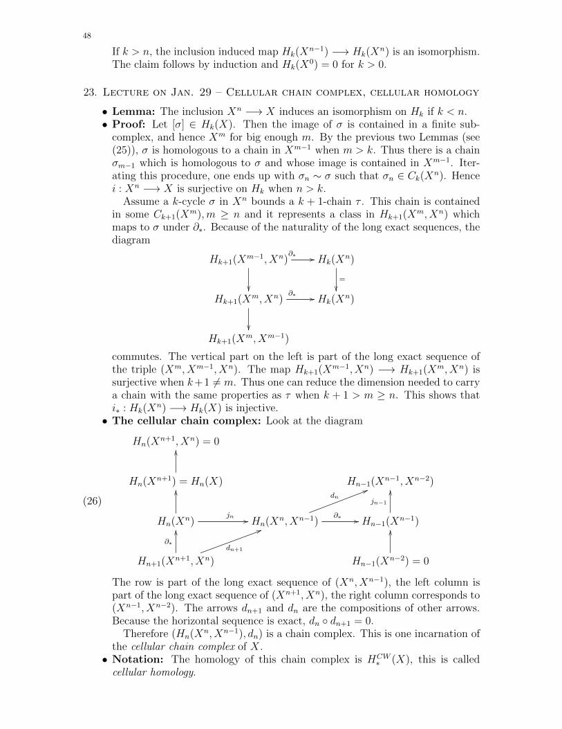
48

If k > n, the inclusion induced map Hk(Xn−1) −→ Hk(X

n) is an isomorphism.The claim follows by induction and Hk(X

0) = 0 for k > 0.

23. Lecture on Jan. 29 – Cellular chain complex, cellular homology

• Lemma: The inclusion Xn −→ X induces an isomorphism on Hk if k < n.• Proof: Let [σ] ∈ Hk(X). Then the image of σ is contained in a finite sub-

complex, and hence Xm for big enough m. By the previous two Lemmas (see(25)), σ is homologous to a chain in Xm−1 when m > k. Thus there is a chainσm−1 which is homologous to σ and whose image is contained in Xm−1. Iter-ating this procedure, one ends up with σn ∼ σ such that σn ∈ Ck(Xn). Hencei : Xn −→ X is surjective on Hk when n > k.

Assume a k-cycle σ in Xn bounds a k + 1-chain τ . This chain is containedin some Ck+1(Xm),m ≥ n and it represents a class in Hk+1(Xm, Xn) whichmaps to σ under ∂∗. Because of the naturality of the long exact sequences, thediagram

Hk+1(Xm−1, Xn)∂∗ //

��

Hk(Xn)

=

��Hk+1(Xm, Xn)

∂∗ //

��

Hk(Xn)

Hk+1(Xm, Xm−1)

commutes. The vertical part on the left is part of the long exact sequence ofthe triple (Xm, Xm−1, Xn). The map Hk+1(Xm−1, Xn) −→ Hk+1(Xm, Xn) issurjective when k+1 6= m. Thus one can reduce the dimension needed to carrya chain with the same properties as τ when k + 1 > m ≥ n. This shows thati∗ : Hk(X

n) −→ Hk(X) is injective.• The cellular chain complex: Look at the diagram

Hn(Xn+1, Xn) = 0

Hn(Xn+1) = Hn(X)

OO

Hn−1(Xn−1, Xn−2)

Hn(Xn)jn //

OO

Hn(Xn, Xn−1)∂∗ //

dn55

Hn−1(Xn−1)

jn−1

OO

Hn+1(Xn+1, Xn)

∂∗

OO

dn+1

55

Hn−1(Xn−2) = 0

OO

(26)

The row is part of the long exact sequence of (Xn, Xn−1), the left column ispart of the long exact sequence of (Xn+1, Xn), the right column corresponds to(Xn−1, Xn−2). The arrows dn+1 and dn are the compositions of other arrows.Because the horizontal sequence is exact, dn ◦ dn+1 = 0.

Therefore (Hn(Xn, Xn−1), dn) is a chain complex. This is one incarnation ofthe cellular chain complex of X.• Notation: The homology of this chain complex is HCW

∗ (X), this is calledcellular homology.

49

• Theorem: HCW∗ (X) ' H∗(X).

• Proof: We use three previous Lemmas and the diagram (26).– From the left vertical row: Hn(X) ' Hn(Xn)/image(∂∗ : Hn+1(Xn+1, Xn) −→Hn(Xn)).

– Since Hn(Xn−1) = 0, the map jn is injective, i.e. image(∂∗) is mappedisomorphically of image(jn ◦ ∂∗) = image(dn+1).

– jn−1 is injective. Hence ker(dn) = ker(∂∗).

Now one can read of Hn(X) ' ker(dn)image(dn+1)

• Corollary: The homology of a finite CW -complex is finitely generated, ifthere are no n-cells, then Hn(X) = 0. If there are k n-cells, then Hn(X) canbe generated by at most k elements.• Corollary: Assume X2n+1 ' X2n for all n. H2n+1(X) = 0 and H2n(X) is free

Abelian, the rank of H2n(X) coincides with the number of 2n-cells.• Example: This Corollary is tailored to suit the following example. There are

other instances where it works.

Hk(CPn) '{

0 k odd or k > 2n or k < 0Z 0 ≤ k ≤ 2n even

Hk(HPn) '

0 k > 4n or k < 00 k not a multiple of 4Z 0 ≤ k ≤ 4n divisible by 4

• Description of Hn(Xn, Xn−1): This is isomorphic to a Abelian group gener-ated by the n-cells in X.• Description of dn: Let enα be a n-cell, these cells represent a basis ofHn(Xn, Xn−1).

In terms of this basis

(27) dn(enα) =∑

en−1β (n−1)-cell

deg(ϕα : ∂Dn

α −→ Xn−1/(Xn−1 \ en−1β )

)en−1β .

where ϕα is the attaching map of enα.• Proof: n = 0: There are no −1-cells, so d0 is zero.

n = 1: Each one cell e1α corresponds to a generator of H1(X1, X0), it is

mapped the difference of the end points.n > 1: Again, one looks at a diagram. φα is the characteristic map of the

cell enα and ϕα its restriction to the boundary of Dnα. qβ : Xn−1/Xn−2 −→ Sn−1

β

collapes all points in the complement of en−1β to a point and identifies the result

with Dn−1β /∂Dn−1

β = Sn−1β via the (inverse of the) characteristic map of en−1

β .

We use n ≥ 2 for the bottom right isomorphism (the pair (Xn−1, Xn−2) isgood).

Hn(Dnα, ∂D

nα)

∂∗

'//

φα

��

Hn−1(∂Dnα)

ϕα

��

∆αβ // Hn−1(Sn−1β )

Hn(Xn, Xn−1)∂∗ //

dn ))

Hn−1(Xn−1)

jn−1

��

Hn−1(Xn−1/Xn−2)

qβ∗

OO

Hn−1(Xn−1, Xn−2)

'

55

50

∆αβ is the map that makes everything commute. Since n− 1 > 0, the reducedhomologies in the right column coincide with the non-reduced versions. Bydefinition of the degree,

∆αβ[∂Dnα] = deg

(ϕα : ∂Dn

α −→ Xn−1/(Xn−1 \ en−1β )

)[Sn−1β ]

• Remark: The above two descriptions would allows us to define the cellularchain complex without reference to singular homology. The cellular chain com-plex is very amenable to computations. The non-trivial lesson from the abovediscussion is that homeomorphic CW-complexes have isomorphic cellular ho-mology.• Computation of degrees from local data: In order to use the cellular

chain complex, one needs to be able to compute the degree effectively. Here isa method that works under very mild topological assumptions.

Assume that f : Sn −→ Sn, n ≥ 2, is continuous and y ∈ Sn has finitef−1(y) = {x1, . . . , xm}. Fix a neighborhood V of y and pairwise disjoint neigh-borhoods Ui of xi such that f(Ui) ⊂ V .

There are obvious inclusions: (Ui, Ui \xi) −→ (Sn, Sn \xi) induces an iso. onhomology by excision. The same is true for (V, V \ y) −→ (Sn, Sn \ y). Then

Hn(Ui, Ui \ xi)f∗ //

'��

Hn(V, V \ y)

'��

Hn(Sn, Sn \ xi)f∗ // Hn(Sn, Sn \ y)

The lower map is multiplication with an integer, the local degree of f at xi.This means that

f∗([Ui, Ui \ xi]) = deg(f, xi)[V, V \ y])

where [Ui, Ui \xi] respectively [V, V \ y] is a generator of Hn(Ui, Ui \xi) respec-tively Hn(V, V \ y). These generators (there is a choice which would affect thesign of the local degree) are related via

Hn(Sn) −→ji∗ Hn(Sn, Sn \ xi)←−' Hn(Ui, Ui \ xi)Hn(Sn) −→jy∗ Hn(Sn, Sn \ y)←−' Hn(V, V \ y)

where the arrows from right to left are excision isomorphisms (induced byinclusions), ji : Sn −→ (Sn, Sn \ xi), and iy : Sn −→ (Sn, Sn \ y). For fixed ilet

ki : (Ui, Ui \ xi) −→ (Sn, Sn \ xi)

be the inclusion. Then, by excision and disjoint union

Hn

(⋃i

Ui,⋃i

(Ui \ xi)

)'⊕i

Hn(Ui, Ui \ xi) −→⊕iki∗ Hn(Sn, Sn \ f−1(y))

is an isomorphism. Because of the long exact sequence of the pair (Sn, Sn \ y),the inclusion (Sn, ∅) −→ (Sn, Sn \ y) induces an isomorphism Hn(Sn) −→

51

Hn(Sn, Sn \ y). Consider the diagram⊕iHn(Ui, Ui \ xi)

⊕ki∗'��

induced by f// Hn(V, V − y)

'��

Hn(Sn, Sn \ f−1(y))f∗ // Hn(Sn, Sn \ y)

Hn(Sn)f∗ //

j

OO

Hn(Sn)

'

OO(28)

The lowest line is multiplication by the degree, each summand in the top line ismultiplied with the local degree. In order to finish, we need to express j([Sn])in terms of the direct sum decomposition of Hn (

⋃i Ui,

⋃i(Ui \ xi)).

Let i ∈ {1, . . . ,m} be fixed. By the long exact sequence of the pair (Sn, Sn \xi) the inclusion induces an isomorphism ji : Hn(Sn) −→ Hn(Sn, Sn \ xi). Theinclusion (Sn, Sn \ f−1(y)) −→ (Sn, Sn \ xi) fits into

(∪iUi,∪i(Ui \ xi))

��uu(Sn, Sn \ xi) (Sn, Sn \ f−1(y))oo

Sn

OOii

On homology, the top left arrow induces a projection onto the i-th summand.Thus the image of a fixed generator [Sn] ∈ Hn(Sn) is∑

i

ji∗([Sn]).

We can now compute the degree in terms of local degrees as follows (f∗ refersto maps induced by f , these may differ from line to line, iy is the inclusionSn −→ (Sn, Sn \ y)). From (28) we get

iy∗f∗([Sn]) = deg(f)iy∗([S

n])

= f∗(∑i

ji∗[Sn]) =

∑i

deg(f, xi)iy∗[Sn])

=

(∑i

deg(f, xi)

)iy∗([S

n]).

Therefore

(29) deg(f) =∑i

deg(f, xi)

• Example: We can finally compute H∗(RPn). Recall that X = RPn has aCW-structure such that

– Xk = RPk = {[x0 : . . . : xk : 0 . . . : 0]} ⊂ RPn for 0 ≤ k ≤ n,– Xk+1 = Xk ∪ ek+1 when 0 ≤ k + 1 ≤ n,

– the attaching map ϕk : ∂Dk+1

= Sk −→ Xk = RPk is the two foldcovering (universal for k > 1).

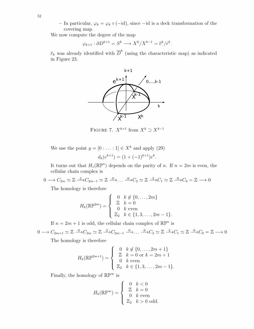
52

– In particular, ϕk = ϕk ◦ (−id), since −id is a deck transformation of thecovering map.

We now compute the degree of the map

ϕk+1 : ∂Dk+1 = Sk −→ Xk/Xk−1 = ek/ek.

ek was already identified with Dk

(using the characteristic map) as indicatedin Figure 23.

Xkk-1X

k-1X

ek+1

k

k+1

0,...,k-1

Figure 7. Xk+1 from Xk ⊃ Xk−1

We use the point y = [0 : . . . : 1] ∈ Xk and apply (29)

dk(ek+1) = (1 + (−1)k+1)ek.

It turns out that H∗(RPn) depends on the parity of n. If n = 2m is even, thecellular chain complex is

0 −→ C2m ' Z −→·2 C2m−1 ' Z −→·0 . . . −→·0 C2 ' Z −→·2 C1 ' Z −→·0 C0 = Z −→ 0

The homology is therefore

Hk(RP2m) =

0 k 6∈ {0, . . . , 2m}Z k = 00 k even

Z2 k ∈ {1, 3, . . . , 2m− 1}.

If n = 2m+ 1 is odd, the cellular chain complex of RPn is

0 −→ C2m+1 ' Z −→·0 C2m ' Z −→·2 C2m−1 −→·0 . . . −→·0 C2 ' Z −→·2 C1 ' Z −→·0 C0 = Z −→ 0

The homology is therefore

Hk(RP2m+1) =

0 k 6∈ {0, . . . , 2m+ 1}Z k = 0 or k = 2m+ 10 k even

Z2 k ∈ {1, 3, . . . , 2m− 1}.

Finally, the homology of RP∞ is

Hk(RP∞) =

0 k < 0Z k = 00 k even

Z2 k > 0 odd.

53

• Definition: Let X be a topological space. The k-th Betti number of X is

bk(X) = rank(Hk(X)) ∈ N0 ∪ {∞}.The rank of an Abelian group is the number of generators of a maximal freeAbelian subgroup.• Definition: Let X be a finite (or, equivalently, compact) CW-complex with ci

cells in dimension i. The Euler characteristic of X is

χ(X) =∑i

(−1)ici.

• Theorem: χ(X) =∑

i(−1)ibi(X). In particular, χ(X) is a topological invari-ant and does not depend on the cell structure.• Proof: Consider the cellular chain complex of X:

0 −→ CCWn −→dn CCW

n−1 −→dn−1 . . . −→ CCW1 −→d1 CCW

0 −→ 0.

For all k there are short exact sequences

0 −→ Bk = {k − boundaries} −→Zk = {k − cycles} −→ Hk −→ 0

0 −→ Zk −→Ck −→ Bk−1 −→ 0.

The second sequence implies rank(Ck) = rank(Zk) + rank(Bk−1). The firstimplies bk(X) = rank(Zk)− rankBk. Therefore,

χ(X) =∑i

(−1)ici =∑i

(−1)i(rank(Zi) + rank(Bi−1))

=∑i

(−1)i(bi(X) + rank(Bi) + rank(Bi−1))

=∑i

(−1)ibi(X).

• Remark: Let X −→ X be a n-sheeted cover of a compact CW-complex. Then

X has a CW-structure such that the restriction of the covering map to each

cell of X is a homeoomorphism onto a cell of X. Hence χ(X) = nχ(X). Thereis no nice relationship between homology groups of a space and its covers.• Theorem (Mayer-Vietoris): Let A,B ⊂ X be open sets such that A∪B =X. Then there is a long exact sequence

. . . −→ Hi(A ∩B) −→ Hi(A)⊕Hi(B) −→ Hi(X) −→∂∗ Hi−1(A ∩B) −→ . . .

[σ] 7−→ (iA∩B→A∗[σ],−iA∩B→B∗[σ])

([α], [β]) 7−→ [iA∗α + iB∗β]

(30)

• Proof: Consider the chain complex CU∗ (X) for U = {A,B}. There is a short

exact sequence

0 −→ Cn(A ∩B) −→ Cn(A)⊕ Cn(B) −→ CUn(X) −→ 0

for all n and the maps involved are chain maps. The corresponding long exactsequence is of the form in 30, the only non-elementary fact used is that theinclusion (CU

∗ (X), ∂) −→ (C∗(X), ∂) is a chain homotopy equivalence (opencover on 40) . It induces an isomorphism on homology.• Remark: This is frequently applied to sets A,B covering X which are not

necessarily open when there are open sets A′ ⊃ A and B′ ⊃ B such the smallerset is a deformation retract of the larger one.

54

• Remark: A similar sequence exists in reduced homology, one uses

0 // C0(A ∩B)

ε

��

// C0(A)⊕ C0(B) //

ε⊕ε��

CU∗ (X) //

ε

��

0

0 // Z // Z⊕ Z // Z // 0

n � // (n,−n)

(a, b) � // (a+ b)

to augment the chain complex.

• Theorem (Jordan non-separation): Let h : Dk −→ Sn be an embedding

and k ≤ n. Then

Hi(Sn \ h(Dk)) = 0 for all i

• Proof: By induction on k. The base case k = 0 is obvious. Assume that thestatement is proved for k − 1 and let Dk = Ik = Dk−1 × I. We write

A = Sn \ h(Dk−1 × [0, 1/2]) B = Sn \ h(Dk−1 × [1/2, 1]).

Both sets are open. Then A ∪ B = Sn \ h(Dk−1 × {1/2}) and A ∩ B =Sn \ h(Dk). By the Mayer-Vietoris sequence and the inductive hypothesis

H∗(Dk−1 × {1/2}) = 0

Hi(A ∩B) −→ Hi(A)⊕ Hi(B)

is an isomorphism. If there is [σ] 6= 0 ∈ Hi(A ∩ B), then σ 6= 0 in Hi(A)

or Hi(B) (up to sign the maps in the Mayer-Vietoris sequence are induced byinclusions).

Assume σ 6= 0 in Hi(A = Sn \ h(Dk−1 × [0, 1/2]). Iterating this process wefind intervals [ai, bi] ⊂ I such that bi − ai = 2−i, [ai, bi] ⊂ [ai−1, bi−1] such that

σ 6= 0 ∈ Hi(Sn \ h(Dk−1 × [ai, bi]) for all i.

By induction, σ = 0 in Hi(Sn\h(Dk−1×a∞)) with a∞ = ∩i[ai, bi]. Then there

is a i+1-chain τ in Sn\h(Dk−1×a∞) such that ∂τ = σ. The space h(Dk−1×a∞)is compact, therefore τ is a chain in the complement of an open neighborhoodof h(Dk−1 × a∞). This complement is contained in the complement of one ofthe sets h(Dk−1 × [ai, bi]) where σ is not zero. This is a contradiction.• Remark: The complement of an embedded closed ball in Sn has the homology

of a ball. This does not mean that it is homeomorphic/homotopy equivalentto a ball. For n = 2 this is true, in higher dimension it is not.• Theorem: Let h : Sk −→ Sn be an embedding. Then

Hi(Sn \ h(Sk)) =

{Z i = n− k − 10 otherwise.

• Proof: By induction. For k = 0, Sn \ h(S0) is homeomorphic to Sn−1 × R.The theorem is true in this case.

Assume that k > 0 and let Sk = D+ ∪ D− where D±0 = {±x0 > 0} arediscs. Then by the Mayer-Vietoris sequence applied to A = Sn \ h(D+) and

55

B = Sn \ h(D−)

0 = Hi(A)⊕ Hi(B) −→ Hi(A ∪B) −→ Hi−1(A ∩B) −→ 0

as long as i− 1 ≥ 0. The claim follows by induction.• Remark: This implies the generalized Jordan curve theorem: The comple-

ment of codimension-1-sphere in Sn consists of two open homology balls. Thecomplement has two path connected components.• Theorem (Invariance of domain): Let U ⊂ Rn be an open set and f :U −→ Rn continuous and injective (for example a homeomorphism). Thenh(U) ⊂ Rn is open.• Proof: Sn \ {pt} is homeomorphic to Rn. We will show that h(U) is open inSn. Let x ∈ U and Dn ⊂ U a close ball containing x in its interior. Then ∂Dn

is a sphere and h(∂Dn) decomposes Dn in two path components, one of themis h(Dn \ ∂Dn) and homeomorphic to an open ball, the other is Sn \ h(Dn).Their union is open since h(∂Dn) is compact.

We show that h(Dn \ ∂Dn) is open. Let y ∈ h(Dn \ ∂Dn). There is anopen ball V around y in Sn \ h(∂Dn). Then V lies in the same path connectedcomponent of Sn \ h(∂Dn) as y.• Remark: We defined the singular chain complex using a chain complex (Ci)

whose elements were of the form∑

j ajσj ∈ Ci where σj are singular i-simplicesand aj ∈ Z. Instead of Z, one can use any other Abelian group, for example G =Z2. One then writes Ci(X;G). When one reinterprets the boundary operatorby viewing (−1) as element in Aut(G), then everything we have discussed so fargoes through without changes. The homology of a point is then H0(pt;G) = G,and the homology groups of the spheres change accordingly.• Definition: The homology of the resulting chain complex is H∗(X;G).• The reduced chain complex is defined using the map ε : C0(X;G) −→ G defined

by summing the coefficients. The homology of the reduced chain complex with

coefficients in G is H∗(X;G).• Lemma: Let ϕ : G1 −→ G2 be a morphism of Abelian groups. The inclusionϕ : Ci(X,G1) −→ Ci(X,G2) is a chain map. For a continuous map f : X −→Y ,

Hi(X;G1)ϕ //

f∗��

Hi(X;G2)

f∗��

Hi(Y ;G1)ϕ // Hi(Y ;G2).

commutes.• Consequence: Let f : Sn −→ Sn be a continuous map. Then f : Hn(Sn;G) −→Hn(Sn;G) is multiplication with an integer m (viewed as endomorphism of G,i.e. m · g = g + g + . . .+ g).• Proof: For g ∈ G, there is an morphism ϕg : Z −→ G defined by 1 → g. By

the previous naturality lemma, f∗(g) = f∗(ϕg(1)) = ϕg(f∗(1)) = ϕg(m) = g ·m.This works for all g with the same m.• Remark: Using the previous Lemma, one obtains a cellular chain complex

whose homology is H∗(X;G). The chain groups CCWi (X,G) are ⊕G, with one

copy of G for each i-cell and the boundary operator is defined by (27).• Example: The cellular chain complex of RPn with coefficients in Z2: For the

standard CW-structure Ck(RPn;Z2) = Z2 iff 0 ≤ k ≤ n and 0 otherwise. All

56

differentials are zero. Then

Hk(RPn;Z2) '{

Z2 0 ≤ k ≤ n0 otherwise

• Proposition: Let f : Sn −→ Sn be continuous such that f(−x) = −f(x).Then the degree of f is odd.

• Preliminaries: Let pr : X −→ X be a 2-sheeted covering. This is automat-ically normal,, we denote the non-trivial deck transformation by ϕ. Considerthe short exact sequence

0 −→ Cn(X;Z2) −→τ Cn(X;Z2) −→pr∗ Cn(X;Z2) −→ 0

where τ is defined as follows. For a singular n-simplex in X we choose a lift

σ : ∆n −→ X such that pr ◦ σ = σ. Then

τ(σ) = σ + ϕ∗(σ).

This determines τ on general chains by linearity and τ is a chain map. Thusthere is an associated long exact sequence, the map induced by τ is a transfermap, the associated long exact sequence is a transfer sequence.• Proof of the Proposition: Consider the covering pr : Sn −→ RPn. Since

f(−x) = −f(x), f induces a map f : RPn −→ RPn. We need to understand

how f , f interact with the short exact sequence: Using the definition of τ , onecan check that the diagram

0 // Ci(RPn;Z2)τ //

f∗��

Ci(Sn;Z2)

pr∗ //

f∗��

Ci(RPn;Z2) //

f∗��

0

0 // Ci(RPn;Z2)τ // Ci(S

n;Z2)pr∗ // Ci(RPn;Z2) // 0

commutes. By naturality of the long exact sequence there is map from thetransfer sequence to itself:

H1(Sn;Z2) //

f∗��

H1(RPn;Z2) //

f∗��

H0(RPn;Z2)τ∗ //

f∗��

H0(Sn;Z2)pr∗ //

f∗��

H0(RPn;Z2)

f∗��

H1(Sn;Z2) // H1(RPn;Z2) // H0(RPn;Z2)τ∗ // H0(Sn;Z2)

pr∗ // H0(RPn;Z2)

The right-most map pr∗ is an isomorphism, so the map preceding it must bezero. Therefore, the connecting morphism H1(RPn;Z2) −→ H0(RPn;Z2) is

sujective, hence it is an isomorphism. Moreover, the map f∗ : H0(RPn;Z2) −→H0(RPn;Z2) is an isomorphism. Hence f∗ : H1(RPn;Z2) −→ H1(RPn;Z2) is anisomorphism.

Inductively, one obtains that f∗ : Hn(RPn;Z2) −→ Hn(RPn;Z2) is an iso-morphism. Finally, look at

Hn+1(RPn;Z2) = 0 //

��

Hn(RPn;Z2) //

f∗��

Hn(Sn;Z2) = Z2//

f∗��

Hn(RPn;Z2)

f∗��

Hn+1(RPn;Z2) = 0 // Hn(RPn;Z2) // Hn(Sn;Z2) = Z2// Hn(RPn;Z2)

The horizontal maps in the middle are injective, hence they are isomorphisms.Hence, f∗ is an isomorphism. We have shown that it is also the multiplicationwith an integer, which must be odd.

57

Using the morphism ϕ : Z −→ Z2 of coefficient groups we conclude, that thedegree of f is odd.• Corollary (Borsuk-Ulam): Let g : Sn −→ Rn be a continuous map. Then

there is a point x such that f(x) = f(−x).• Proof: Assume not and consider

f : Sn −→ Sn−1

x 7−→ g(x)− g(−x)

‖g(x)− g(−x)‖.

The restriction of this map to the equator has the symmetry property neededfor the previous proposition. Therefore, it has odd degree. However, thisrestriction is null-homotopic (shrink Sn−1 in one of the hemispheres), so thedegree would be zero. This is a contradiction.• Remark: There is a strong relationship between H∗(X) and H∗(X;A), the

corresponding theorem is the universal coefficient theorem. This is for nextsemester. Just like the study of C∗ = Hom(C∗,Z) and a ring structure on theresulting cohomology H∗(X).

References

[Br] G. Bredon, Topology and Geometry, Springer GTM 139.[BrtD] T. Brocker, T. tom Dieck, Representations of compact Lie groups, Graduate Texts in Math-

ematics 98, Springer 2003.[Cox] D. A. Cox, Galois theory, 2nd edition (2012), Wiley.[Do] C. H. Dowker, Topology of metric complexes, Amer. J. Math. 74, (1952), 555–577.

[Ha] A. Hatcher, Algebraic Topology, Cambridge Univ. Press 2002, available online3 https://

www.math.cornell.edu/~hatcher/

[Hu] D. Husemoller, Fibre Bundles , third ed. 1994, Springer.[Ja] K. Janich, Topologie, Springer.[Sch] H. Schubert, Topologie, Teubner 1964.[StZ] R. Stocker, H. Zieschang, Algebraische Topologie, Teubner 1994.[Wa] W. Walter, Analysis 2, 3. Auflage, Springer.

3there are slight differences between the printed and the online versions