Topological methods in surface dynamics
76
TOPOLOGY AND ITS Topology and its Applications 58 (1994) 223-298 APPLICATIONS Topological methods in surface dynamics Philip Boyland ’ Institute for Mathematical Sciences, SUNY at Stony Brook, Stony Brook, NY I 1794, USA Received 16 May 1994 Abstract This paper surveys applications of low-dimensional topology to the study of the dynamics of iterated homeomorphisms on surfaces. A unifying theme in the paper is the analysis and application of isotopy stable dynamics, i.e. dynamics that are present in the appropriate sense in every homeomorphism in an isotopy class. The first step in developing this theme is to assign coordinates to periodic orbits. These coordinates record the isotopy, homotopy, or homology class of the corresponding orbit in the suspension flow. The isotopy stable coordinates are then characterized, and it is shown that there is a map in each isotopy class that has just these periodic orbits and no others. Such maps are called dynamically minimal representatives, and they turn out to have strong global isotopy stability properties as maps. The main tool used in these results is the Thurston-Nielsen theory of isotopy classes of homeomorphisms of surfaces. This theory is outlined and then applications of isotopy stability results are given. These results are applied to the class rel a periodic orbit to reach conclusions about the complexity of the dynamics of a given homeomorphism. Another application is via dynamical partial orders, in which a periodic orbit with a given coordinate is said to dominate another when it always implies the existence of the other. Applications to rotation sets are also surveyed. Keywords: Dynamical systems; Periodic orbits; Thurston-Nielsen theory 0. Introduction Dynamical systems theory studies mathematical structures that are abstractions of the most common scientific models of deterministic evolution. The two main elements in the theory are a space X that describes the possible states or configurations of the system and a rule that prescribes how the states evolve. The mathematical expression of this evolution rule is the action of a group or semi-group on the space. The group is often thought of as time, and dynamical systems theory is usually restricted to the ’ The author was partially supported by NSF Grant No. 431-4591-A. E-mail: [email protected]. 0166.8641/94/$07.00 @ 1994 Elsevier Science B.V. All rights reserved SSDlO166-8641(94)00045-5
-
Upload
paulo-coelho -
Category
Education
-
view
206 -
download
2
Transcript of Topological methods in surface dynamics
TOPOLOGY AND ITS
Topology and its Applications 58 (1994) 223-298
APPLICATIONS
Topological methods in surface dynamics Philip Boyland ’
Institute for Mathematical Sciences, SUNY at Stony Brook, Stony Brook, NY I 1794, USA
Received 16 May 1994
Abstract
This paper surveys applications of low-dimensional topology to the study of the dynamics of iterated homeomorphisms on surfaces. A unifying theme in the paper is the analysis and application of isotopy stable dynamics, i.e. dynamics that are present in the appropriate sense in every homeomorphism in an isotopy class. The first step in developing this theme is to assign coordinates to periodic orbits. These coordinates record the isotopy, homotopy, or homology class of the corresponding orbit in the suspension flow. The isotopy stable coordinates are then characterized, and it is shown that there is a map in each isotopy class that has just these periodic orbits and no others. Such maps are called dynamically minimal representatives, and they turn out to have strong global isotopy stability properties as maps. The main tool used in these results is the Thurston-Nielsen theory of isotopy classes of homeomorphisms of surfaces. This theory is outlined and then applications of isotopy stability results are given. These results are applied to the class rel a periodic orbit to reach conclusions about the complexity of the dynamics of a given homeomorphism. Another application is via dynamical partial orders, in which a periodic orbit with a given coordinate is said to dominate another when it always implies the existence of the other. Applications to rotation sets are also surveyed.
Keywords: Dynamical systems; Periodic orbits; Thurston-Nielsen theory
0. Introduction
Dynamical systems theory studies mathematical structures that are abstractions of
the most common scientific models of deterministic evolution. The two main elements
in the theory are a space X that describes the possible states or configurations of the
system and a rule that prescribes how the states evolve. The mathematical expression
of this evolution rule is the action of a group or semi-group on the space. The group
is often thought of as time, and dynamical systems theory is usually restricted to the
’ The author was partially supported by NSF Grant No. 431-4591-A. E-mail: [email protected].
0166.8641/94/$07.00 @ 1994 Elsevier Science B.V. All rights reserved SSDlO166-8641(94)00045-5
224 P: Boyland/Topology and its Applications 58 (1994) 223-298
cases where the (semi-) group is the non-negative integers, N, the integers, Z, or the
real numbers, R.. In the first two cases one has discrete steps of evolution in time, and
in the latter, continuous evolution. The action of these groups on the space X is realized
by the forward iterates of a non-invertible map, all iterates of an invertible map, and a
flow (i.e. the solution to a differential equation), respectively. In the latter two cases the
evolution can be reversed in time and in the first it cannot.
Since one would hope that most spaces of configurations are at least locally Euclidian,
it is common to restrict attention to dynamics on manifolds. There are thus a variety
of situations to study determined by the dimension of the manifold and the type of
dynamical system. One can also work with holomorphic maps on complex manifolds,
or else restrict to the real case. In addition, within dynamics there are at least three points
of view that can be taken. In the topological theory one studies topological properties
of the orbit structure. The smooth theory uses invariants that can only be defined
using the differentiability and often isolates dynamical phenomenon whose presence
depends on the smoothness of the system. Ergodic theory studies statistical and measure
theoretic aspects of the orbit structure. In the tradition of Klein one could say that the
topological theory studies those structures that are invariant under continuous changes
of coordinates, the smooth theory those that are invariant under smooth changes of
coordinates, and ergodic theory those that persist under measure isomorphism. As is
typical in mathematics, some of the most interesting questions in the field lie at the
intersection of various points of view.
Within dynamical systems, then, there are many possible theories as determined by
the dimension of the manifold, the type of dynamical system and the point of view. This
paper will focus on the topological theory of the dynamics of iterated homeomorphisms
in real dimension two. For iterates of surface homeomorphisms, orbits are codimension
two, which topologists will recognize as the knotting codimension. This accounts for
the combinatorial character of much of the theory presented here.
There is a useful heuristic in dynamics that says that N-actions in dimension n, behave
roughly like Z-actions in dimension y1+ 1, which in turn, behave roughly like R-actions
in dimension n + 2. One must approach this heuristic with caution. There are always
new phenomena that arise when the dimension is increased even if the size of the group
acting is increased as well. Despite this caution there will be many instances in our
study of iterated homeomorphisms on surfaces when it will be useful to use tools and
examples involving flows on 3-manifolds or involving iterated endomorphisms on the
circle. These examples are given along with some basic definitions in Section 1.
In Section 2 we begin the development of one of the main themes of the paper. The
goal of dynamical systems theory is to understand the orbit structure of a dynamical
system. To further this goal, it is natural to assign a number or other algebraic invariant
to an orbit. In the topological theory this is often accomplished by using an algebraic
object (e.g. a homology or homotopy class) that measures the motion of the orbit around
the manifold. A fair amount of this paper deals with the theory of these invariants for
periodic orbits. The situation for general orbits is considered in Sections 6 and 11.
The material in Sections 2 and 3 concerns three types of invariants for periodic
P BoylandlTopology and its Applications 58 (1994) 223-298 225
orbits. These three invariants measure the isotopy, homotopy, and homology class of the
orbit in the suspension flow. Each invariant is naturally associated with an equivalence
relation, namely, periodic orbits are equivalent if they are assigned the same invariant.
In Section 4 we address the question of which of these invariants are isotopy stable,
i.e. are present in the appropriate sense for every homeomorphism in the isotopy class.
The identification of these classes allows one to assign a collection of invariants to an
isotopy class. The size of this collection gives a lower bound for the complexity of the
dynamics of any element in the class.
The existence of a dynamically minimal representative in an isotopy class is closely
connected with the isotopy stable classes of periodic orbits. A dynamically minimal
representative is a map that just has the dynamics that must be present (i.e. the isotopy
stable dynamics) and nothing more. The existence of these maps for the class of
dynamical systems studied here is given in Section 5. Having obtained a dynamically
minimal representative one then asks about the isotopy stability of the other, non-periodic
orbits of the minimal representative. This leads to the notion of isotopy stability for a
map which is considered in Section 6.
The Thurston-Nielsen theory is undoubtedly the most important tool in the topological
theory of surface dynamics. This theory is outlined on Section 7. It is the Thurston-
Nielsen theory that allows one to understand isotopy stable dynamics on surfaces. The
dynamical minimal models discussed in Section 5 are a refinement of the Thurston-
Nielsen canonical map in the isotopy class. This Thurston-Nielsen form can be computed
via the algorithm of Bestvina and Handel that is summarized in Section 10 (Section 10
was written by T.D. Hall).
It is perhaps not immediately obvious how studying isotopy stable dynamics is useful
in understanding the dynamics of a single homeomorphism. For example, if the home-
omorphism is isotopic to the identity, the isotopy stable dynamics consists of a single
fixed point. The key idea involved in the application of isotopy invariant information
goes back to Bowen [ 161. When the given homeomorphism has a periodic orbit, one
studies the isotopy class rel the periodic orbit. The isotopy stable dynamics in this class
clearly must be present in the given homeomorphism. There are many applications of
this basic idea. In Section 8 we give conditions on a periodic orbit that imply the am-
bient dynamics are complicated, for example, there are periodic orbits with infinitely
many periods.
The implications of the existence of a periodic orbit of certain type is examined more
closely in Section 9 using dynamical order relations. One defines an order relation on
the algebraic invariants assigned to periodic orbits by declaring that one invariant is
larger than a second if whenever a homeomorphism has a periodic orbit of the first type
it has also has one of the second. These order relations are a generalization of the partial
order that occurs in Sharkovski’s theorem about the periods of periodic orbits for maps
of the line.
Instead of connecting the invariants of periodic orbits from isotopic maps, one can
collect together all the invariants associated with all the periodic orbits of single home-
omorphism. This set will encode a great deal of information about the dynamics of the
226 F! BoylandlTopology and its Applicafions 58 (1994) 223-298
homeomorphism. The set of all the invariants of orbits is best understood in the Abelian
theory. The rotation vector measures the rate of rotation of an orbit around homology
classes in the surface. A rotation vector can be assigned to a general orbit that may
not be periodic. The set of all the rotation vectors for a homeomorphism is called its
rotation set. In Section 11 we discuss some of what is known about the rotation sets of
surface homeomorphisms.
1. Basic definitions and examples
This section is devoted to definitions and examples that will be used at various
points in this paper. Although our focus in this paper is the dynamics of iterated surface
homeomorphisms, as is typical in mathematics, knowledge of a broad range of examples
of various dimensions and types will be useful in our study of this more restricted class.
The examples will be studied in further detail at various points in the paper. We begin
by precisely specifying the primary objects of study in this paper.
Standing assumption. Unless otherwise noted, M denotes a compact, orientable two-
manifold (perhaps with boundary). Any self-maps f : M -+ M will be orientation-
preserving homeomorphisms.
1. I. Basic dejinitions
For the purposes of this paper, a dynamical system is a topological space X and a
continuous self map f : X + X. The system is denoted as a pair (X, f). The main
object of study are orbits of points. These are obtained by repeatedly applying the
self-map. If f composed with itself n times is denoted f”, then the orbit of a point
x is o(n, f) = {. . . , f-‘(~) , f-’ (x), x, f(x), f2( x), . . .} when f is invertible, and
4x3 f) = (x7 f(x) 9 f2W 9. . .}, when it is not. If the map is clear from the context an
orbit is denoted o(x).
A periodic point is a point x for which f”(x) = x for some n > 0. The least such
n is called the period of the periodic point. A periodic orbit is the orbit of a periodic
point. Clearly the notions of periodic orbit and periodic point are intimately connected,
but in certain circumstances the distinction between the two concepts is essential. The
set of all periodic points with period n is denoted P,,(f), and the set of points fixed
by f is Fix(f). Note that, in general, Fix( f”) may be larger than P,,(f). A point x is
recurrent if there exists a sequence ni + 00 with f” (x) --) x. The recurrent set is the
closure of the set of recurrent points. In the examples we will study all the interesting
dynamics takes place on the recurrent set.
A dynamical system (X, f) is said to be semiconjugate to a second (Kg) if there
is a continuous onto function h : X + Y with hf = gh. In this case, (Kg) is said to
be a factor of (X, f), and (X, f) is called an extension of (Kg). If the map h is a
homeomorphism, the systems are said to be conjugate. From the topological point of
I? Boyland/Topology and ifs Applications 58 (1994) 223-298 221
view the dynamics of conjugate systems are indistinguishable. If the systems are only
semiconjugate, the dynamics of the extension are at least as complicated as that of its
factor.
There are a number of good general texts on dynamical systems; a sampling is
[3,32,59,109,110,113].
1.2. Subshifts of jinite type
Our first examples are zero-dimensional. The symbolic description of these systems
makes it fairly easy to analyze their dynamics. For this reason they are often used to
model the dynamics of pieces of higher dimensional systems. For more information on
subshifts of finite type see [ 1191 or [ 401.
The first ingredient of these systems is a set of letters forming an “alphabet set”
A, ={1,2,... ,n}. The set of all bi-infinite words in the alphabet is & = A:. The set
& is topologized using the product topology in which case it is a Cantor set. There
is a natural self-homeomorphism c : 2, + &, namely shifting a sequence to the left
by one place. The dynamical system (&,, a) is called the full shift on n symbols. In a
slight abuse of language, sometimes just the space itself is called the full shift.
There are certain shift invariant subsets of the full shift which have a simple finite
description. To construct these so-called subshifts, let B be an n x n matrix with all
entries equal to zero or one, and & consists of those sequences s from &, which contain
consecutive letters si = j and si+t = k for just those j and k for which Bj,k = 1. A more
succinct description of & is {s E Z,, : BSi,Si,, = 1). The dynamical system (A,, U) (or
sometimes just the space &) is called a subshift ofjnite type. It is easy to check that
subshifts of finite type are compact and shift invariant.
The matrix B is called the transition matrix. Subshifts of finite type are also sometimes
called topological Markov chains (see [ 301). The idea here is that the letters in the
alphabet represent various states and an element of the subshift represents the coding of
a single outcome of the process. The symbol ak can follow the symbol aj precisely when
the system can make a transition from the state represented by aj to that represented
by Uk. This happens if and only if the (j, k) th entry in the transition matrix is equal to
one.
Of particular interest are those matrices that are irreducible. These matrices are defined
by the property that for all (i, j), there is an n > 0 so that (B”)ij > 0. In this case the
set of periodic orbits of the system (&, (T) is dense in A,. Further, there is a dense
orbit, and in fact, the set of points whose orbits are dense is a dense-G6 set in A,.
Subshifts of finite type have been studied in great detail. They have a number of
other properties that will be useful here. To present these properties we first need a few
definitions. The topological and measure-theoretic entropies are well known measures
of the complexity of a dynamical system (see [ 119,96,107] for definitions and various
properties). The topological entropy of a map f is denoted htop( f). If ,U is an f- invariant probability measure, then h,(f) is the measure-theoretic entropy of f with
respect to ,u. It turns out that for any such measure ,x, h,(f) < htop( f) . Any measure
228 f? Boyland/Topology and its Applications 58 (1994) 223-298
for which equality holds is called a measure of maximal entropy. Irreducible subshifts
of finite type always have a unique measure of maximal entropy. In addition, the shift is
ergodic with respect to the measure of maximal entropy. This means that invariant sets
have measure zero or one. The Birkhofs ergodic theorem says that if the system (X, T)
is ergodic with respect to the invariant measure ,u, then for any u E L’ (,u),
1 n -c n+l iz0
a(T’(x)) --+ s a@
for p almost every point x E X.
Given a sequence a,, its exponential growth rate is
growth( a,) = lim sup log, (anI
n+cC n
Roughly speaking, a sequence that has exponential growth rate log(A) will grow like
A” as n --f CO. In what follows, we will sometimes consider the exponential growth rate
of periodic orbits by considering Fixm (f) = growth(card(Fix( f”) ). For irreducible
subshifts of finite type this quantity is related to the topological entropy and the spectral
radius of B by
FixW(gIn,) = htop(~l,t,) =log(spec(B)).
An irreducible transition matrix B satisfies the hypothesis of the Perron-Frobenius
theorem and so, in particular, the spectral radius of B is always strictly bigger than one
and thus there is positive topological entropy. Note that fixed points of 8 are created
by transitions from a state back to itself under the nth iterate and are therefore counted
by the trace of B”. Since B has an eigenvalue of largest modulus A > 1, trace( B”) is
growing like A”. This explains the connection of spec( B) to Fixa.
There is a theory of one-sided subshifts ofjnite type that is analogous to the two-sided
theory. In this case one considers only one-sided infinite words from the alphabet set
to get the full one-sided shift on n symbols 2,, + = A;. The shift map is now n-to-one.
Given a transition matrix, one defines the corresponding subshift as in the two-sided
case. Most other features of the two theories are identical.
1.3. Circle endomorphisms
The circle is the simplest manifold that is not simply connected. The rotation number
of a point measures the asymptotic rate at which the orbit goes around the circle. In
Section 11 the rotation number will be generalized to measure the rates of motion
around various loops in a surface. For more information on the dynamics of circle
endomorphisms see [ 1,14,32,3 11.
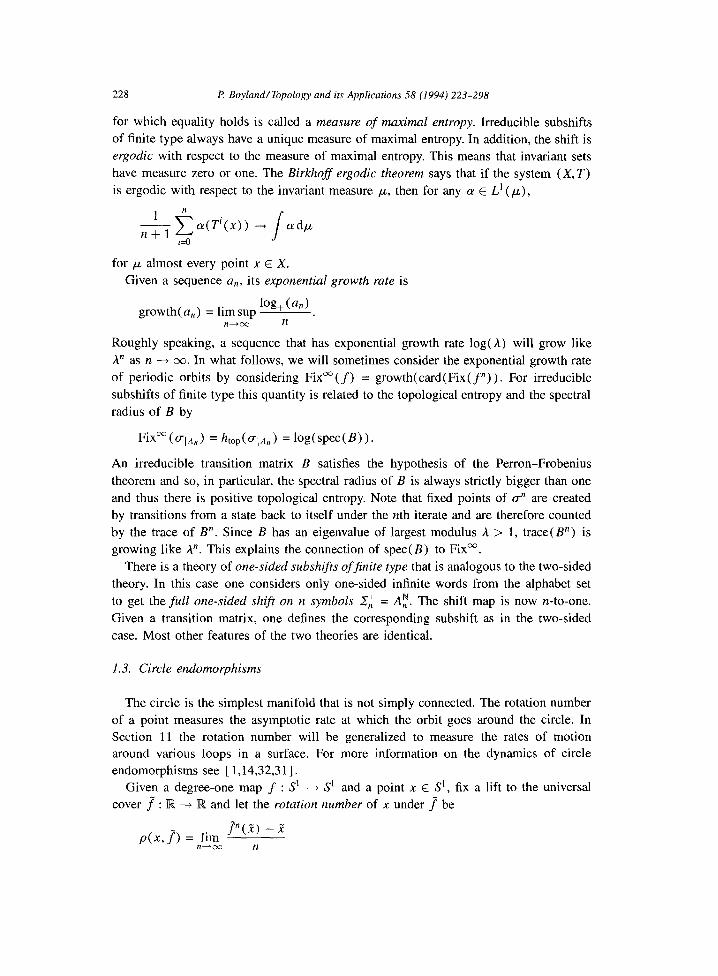
Given a degree-one map f : S’ --f S’ and a point x E S’, fix a lift to the universal
cover f : R -+ R and let the rotation number of x under f be
p(x, J‘) = lim r”(Z) -P
n-03 n

I? Boyland/Topology and its Applications 58 (1994) 223-298 229
2 ’ I I I 1 3 5 2 4
Fig. 1.1. The graph of the lift of the map G,.
when the limit exists, where R E lR is a lift of x. The rotation set is p(f) = {p(x, f) :
x E S’}. The rotation set is always a closed interval. The rotation number of a point
x does not depend on the choice of its lift Z, but changing the choice of the lift of f
will change rotation numbers and the entire rotation set by an integer. This ambiguity
usually does not cause confusion and the rotation set is thus written as a function of f,
p(f), not of J If f is a homeomorphism, then every point has a rotation number, and this number
is the same for all points x E S’. For this reason a circle homeomorphism is said to
have a rotation number rather than a rotation set. If f is not injective, rotation numbers
have features that are analogous to rotation vectors in two-dimensional dynamics. For
example, different orbits can rotate at different asymptotic rates, and there can be points
for which the rotation number does not exist. Another feature is that a periodic orbit
can have rotation number p/q, but have period a multiple of q.
We will now focus on a specific example that will introduce the one-dimensional
analogs of many of the notions that will be used in our two-dimensional examples. Let
G, : S’ + S’ be the piecewise-linear map whose lift is pictured in Fig. 1.1. Let c E S’
denote the point at which the lift has a local maximum. Note that both turning points
are on the same orbit of f and that c has period 5 and p(c) = 2/5. Label the closed
intervals between elements of o(c, G,) as {Ii,. . . ,15} as shown in Fig. 1.3. The crucial
feature of these intervals is that the image of any interval consists of a finite union of
other intervals. This feature makes these intervals what is called a Markov partition for
the map. This notion will be defined more precisely below in the two-dimensional case.
The elements of a Markov partition can be thought of as states in a Markov process.
They allow one to code the orbits by their passage through these states. This allows one
to treat the map as a factor of a one-sided subshift of finite type. There are ambiguities
in the coding of a point whose orbit hits the boundary of a Markov interval. Initially
we will only define the coding away from this bad set X = {x : o(x) n o(c) f @}. To accomplish the coding, for each x E S’ - X, define an element W(x) of 2; by
( W(x) ) n = i if G:(x) E Ii. To get a description of all the possible codes of orbits we
need to compute the transition matrix B of the Markov partition. This matrix is defined
230 P. Boyland/Topology and its Applications 58 (1994) 223-298
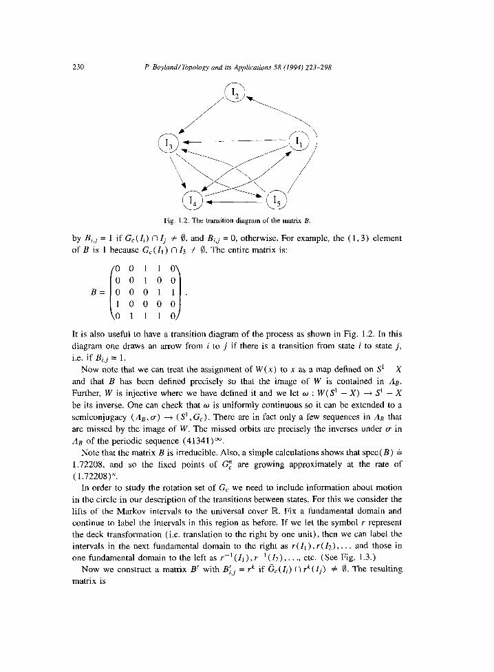
Fig. 1.2. The transition diagram of the matrix B.
by Bi,j = 1 if G, (Ii) c1 Zj Z 8, and Bi,j = 0, otherwise. For example, the ( 1,3) element
of B is 1 because G, (Ii ) fl Zs # 8. The entire matrix is:
00110
00100
B= 0 0 0 1 1 .
i 1
1 0 0 0 0
0 1 1 1 0
It is also useful to have a transition diagram of the process as shown in Fig. 1.2. In this
diagram one draws an arrow from i to j if there is a transition from state i to state j,
i.e. if Bi,j = 1.
Now note that we can treat the assignment of W(x) to x as a map defined on S’ - X
and that B has been defined precisely so that the image of W is contained in &.
Further, W is injective where we have defined it and we let w : W( S’ - X) -+ S’ - X
be its inverse. One can check that w is uniformly continuous so it can be extended to a
semiconjugacy (Aa, g) + (S’ , G,). There are in fact only a few sequences in &i that
are missed by the image of W. The missed orbits are precisely the inverses under g in
& of the periodic sequence (4 1341) M.
Note that the matrix B is irreducible. Also, a simple calculations shows that spec( B) G
1.72208, and so the fixed points of GE are growing approximately at the rate of
( 1.72208)“.
In order to study the rotation set of G, we need to include information about motion
in the circle in our description of the transitions between states. For this we consider the
lifts of the Markov intervals to the universal cover R. Fix a fundamental domain and
continue to label the intervals in this region as before. If we let the symbol r represent
the deck transformation (i.e. translation to the right by one unit), then we can label the
intervals in the next fundamental domain to the right as I( Ii) , r( 12)) . . . and those in
one fundamental domain to the left as I-’ (Ii ) , r-l (12)) . . ., etc. (See Fig. 1.3.)
Now we construct a matrix B’ with Bi,j = rk if G,( Ii) n rk( Ij) # 8. The resulting
matrix is

P. Boyland/Topology und its Applications 58 (1994) 223-298 231
r-l (14) r, I, ‘(I* > r(I, >
5 12 3 4 5 12 3 4 5
r-’ (I,) I, I, I, I, I, 41, > rQ2) r(13) r(I, > Fig. 1.3. The image of the lift of G, is shown above the line. An overline indicates an image.
Fig. 1.4. The transition diagram of the matrix B’.
r 0 0 0 0
0 Y Y r 0
A transition diagram is given in Fig. 1.4. Now the arrows that represent transitions are
labeled with the appropriate power of r.
To obtain rotation number information from these diagrams we need one more def-
inition. If B is the transition matrix for a subshift of finite type, a minimal loop is
a periodic word whose repeating block contains each letter from the alphabet at most
once. The repeating blocks of the minimal loops for our matrix B are 14, 35, 134, 235
and 5413. The crucial observation is that any sequence in the subshift of finite type
can be obtained by the pasting together of minimal loops. This means that the rotation
number of any word can be obtained by knowing the rotation numbers of its constituent
minimal loops.
For example, the minimal loop 14 contains a one transition labeled with an r and
thus the corresponding orbit has rotation number l/2. Similarly, the minimal loop 134
has a single r transition and thus represents a periodic orbit with rotation number l/3.
Thus the concatenated and repeated block 141341 contains two r transitions and yields
a periodic orbit with rotation number ( 1 + 1)/(2 + 3). Thus by using so-called Farey

232 P Boyland/Topology and its Applications 58 (1994) 223-298
arithmetic one can obtain the rotation numbers of all orbits from the pasting structure
of the minimal loops of their sequences in An. In particular, the rotation set of G, is
precisely the convex hull of the rotation numbers of the periodic orbits coming from
minimal loops. It is easy to compute then that G, = [ l/3,1/2].
This technique of encoding information about motion of Markov boxes in the covering
spaces is due to Fried. Theorem 11 .l is a consequence of using the two-dimensional
analogs of these ideas. We also want to comment here on another feature of this example
that has an important two-dimensional analog. If another map of the circle has a periodic
orbit with the same permutation on the circle as that of c under G,, it seems reasonable
that the second map’s dynamics must be at least as complicated as that of G,. This is
true, and in fact, the second map will always have a compact invariant set that has G, as
a factor. Thus, in particular, its entropy will be greater than equal to that of G, and its
rotation set will contain that G,. These are the one-dimensional analogs of Corollaries
7.5(a) and 11.2. To develop a further analog to the pseudoAnosov maps of the two-
dimensional theory (see Section 7), note that we can find a map that is conjugate to G,
but whose slope has a constant absolute value of spec(B). In this case the measure of
maximal entropy is Lebesgue measure. For more remarks on the connection of the one
and two-dimensional theories, see [ 181.
We leave most aspects of our final circle map example as an exercise. The angle
doubling map is a degree-two map of the circle defined by Hd (0) = 28. Show that the
two intervals [0,1/2] and [ l/2,1 ] give a Markov partition for Hd and a semiconjugacy
from the full one-sided shift on two symbols to Hd. As a consequence, show that the
periodic orbits of Hd are dense in the circle and there are points whose orbits are dense.
What is the topological entropy of Hd? Can one make any sense out of rotation numbers
in this case?
1.4. Markov partitions
As we saw in the previous examples, a Markov partition gives a symbolic coding
of a system. We shall use these partitions in a variety of situations and each situation
would require its own definition. Instead we take an operational approach; we simply
state what a Markov partition does and allow the reader to consult the literature for
precise definitions in various cases.
If Y is a compact invariant set for a surface homeomorphism f, a Markov partition
for (I: f) is a finite cover by topological closed disks {RI,. . . , I&}, so that for each
i # j, RiflInt(Rj) =0 and f( Ri) n Rj is either empty or connected. Further, if B is
the k x k matrix (called the transition matrix) defined by Bi,j = 1 if f( Ri) fl Rj # 8,
and 0 otherwise, then (An, a) is semiconjugate to (Y f) . The semiconjugacy is one-to-
one except at points whose orbits intersect the boundary of some Ri. On these points
the semiconjugacy is finite-to-one. The semiconjugacy is defined using the inverse of
the coding of points as was done with the map W in Section 1.3. In particular, for
any sequence ai of elements from { 1,2,. . . , k}, ni,, f’(Int( R,) ) is either empty or a
single point.
P Boyland/Topology and its Applications 58 (1994) 223-298 233
1.5. Linear toral automorphisms
Next we discuss homeomorphisms on the two torus T* = S’ x S’ which are induced
by linear maps acting on the universal cover of the torus, IR*. The deck transformations
of this cover are {T,,, : (m,n) E Z”} where T,,,,(x,y) = (x+m,y +n). A matrix
C E SLz(Z), i.e. C is a 2 x 2 matrix with integer entries whose determinant is equal
to one, always descends to a homeomorphism fc : T* + T*. This is because for any
(m, n), C TV,, = T,,~,,I C where (m’,n’) = C(f).
We will be using two specific instances of this construction. Let Hf denote the
homeomorphism induced by the matrix
0 cf= ,’ _1 ( >
and HA denote the homeomorphism induced by
CA = 2 1 ( > 1 1.
The dynamics of Hf are fairly simple. There are exactly four fixed points. These are
the points on T* that are the projections of the points (O,O), ( l/2,0), (0, l/2), and
( l/2,1/2). Every other point has period 2 and in fact, Hf” = Id (the subscript “f” stands
for finite-order).
The dynamics of HA are considerable more complicated and there is a Markov
partition that codes orbits on the entire torus. The crucial data in constructing the
partition are the eigenvalues and eigenvectors of C; At = A = i(3 + v%), A2 = l/A =
i(3 - &), ut = (i(l + &),I), and uz = (i(1 - &),l>. The vectors u1 and u:!
are usually called the unstable and stable directions, respectively, because these are the
directions of the linear expansion and contraction, and thus give the directions of stable
and unstable manifolds for periodic points.
The Markov partition is constructed using these stable and unstable directions. The
actual details of the construction are somewhat complicated to describe, so we refer the
reader to [ 1091 or [ 321. It should be mentioned that there is a standard technique for
constructing a subshift of finite type from any matrix of positive integers, not just from
matrices of zeros and ones as considered here (see [ 40, p. 191) . Using this construction
the subshift modeling the dynamics of HA is constructed using the matrix CA.
The semiconjugacy with the irreducible subshift of finite type implies that periodic
orbits are dense (in fact, it is easy to check that set of periodic orbit is exactly the
projection to T* of Q2). There is also a dense orbit which implies that the recurrent
set is all of T*. Lebesgue measure is HA-invariant since the matrix CA has determinant
equal to one, and it is the unique measure of maximal entropy.
Any C E SLz(Z) with 1 trace(C) 1 > 2 will induce a toral automorphism that has a
Markov partition and will be a factor of a irreducible subshift of finite type. These maps
are often called hyperbolic toral automorphisms. In this language the finite-order map
Hf is called elliptic. Hyperbolic toral automorphisms are the simplest case of Anosov

234 P Boyland/Topology and its Applications 58 (1994) 223-298
Fig. 1 S. A saddle fixed point and its blow up
diffeomorphisms (see [ 1131, [ 1091, or [38] ). (The subscript “A” in HA stands for
Anosov.)
1.6. Blowing up periodic orbits
It is often useful to use a diffeomorphism on a closed surface to obtain one on a
surface with boundary by replacing periodic points with boundary components. This is
accomplished through the procedure of blowing up. It is a local operation so it suffices to
describe the operation in the plane. Assume that f : IK2 --+ Et2 a homeomorphism that is
differentiable at the origin and f(0) = 0. Let R’ be the surface obtained by removing the
origin from the plane and replacing it by a circle, thus R’ = [ 0,~) x S’. After expressing
f : El2 + Et2 in polar coordinates, we define f’ : R’ -+ R’ via f’( r, 0) = f(r, 0) if
Y > 0 and f’( 0,0) = Dfc( 0)) where we have used Dfn to denote the map induced on
angles by the derivative of f at zero. Its clear that f’ will be a homeomorphism. We
can use a similar procedure to blow up along a periodic orbit of a diffeomorphism. An
illustration is given in Fig. 1.5.
1.7. Mapping class and braid groups
If two homeomorphisms fc and fi are isotopic, this is denoted by fa E fi. If
there is a specific isotopy given it is written ft : fo N fl. If M is a closed surface,
then the collection of isotopy classes of orientation preserving homeomorphisms on
M with the operation of composition is called the mapping class group of M, and is
denoted MCG( M). An isotopy class is sometimes called a mapping class. If M has
boundary, there are two choices. The first is to just allow mapping classes consisting
of homeomorphisms that are the identity on the boundary and isotopies that fix the
boundary pointwise. This mapping class group will be denoted MCG( M, aM>. The
second choice is to allow the boundary to move under both the homeomorphisms and
the isotopies. This case will be denoted as MCG( M). In dynamical applications it is
often useful to consider isotopy classes rel a finite set A, i.e. all homeomorphisms must

P. Boyland/Topology and its Applications 58 (1994) 223-298 235
Fig. 1.6. The element rrlv;‘q? from B4.
leave A invariant, and all isotopies are rel A. This group is denoted MCG( M rel A).
If there is both boundary and a distinguished set of points A, then the notations are
combined. For example MCG( 0’ rel A, dD*) is all isotopies classes of the disk that fix
the boundary pointwise and leave the set A invariant.
The mapping class groups have been extensively studied, see for example [ 10,751.
The mapping class group is sometimes called the modular group of the surface in analogy
with the fact that SL2 (Z) is the mapping class group of the torus. The construction in
Section 1.5 shows how to get a homeomorphism of the torus and thus a mapping class
from an element of SL2( Z) . The two groups are isomorphic because each mapping
class contains exactly one linear model.
Another mapping class group that is fairly well understood is MCG( D* rel A, dD*)
These groups can be identified with Artin’s braid group on n-strings, B,, as follows (see
[lo] for more details). We will just describe the correspondence for the braid group on
4 strings, the other cases being similar.
The elements of the braid groups are geometric braids. Braids that are isotopic are
considered equivalent. The group B4 has generators ,f’, c$‘, and (T$‘. The generators
are combined into words by placing one below the other. Thus Fig. 1.6 shows the -1 element (~1 cr2 ~3. The relations in B4 are (~1~3 = gj~t, UIU~(T~ = (~2~1~2, and
~21~3~2 = ~3~2~3. The commutativity relation is clear geometrically, the other relations
are somewhat more subtle (see Fig. 2 in [ lo] ).
In connecting the braid groups with mapping class groups, we once again focus on
BJ. Let A = {Al,A2.A3, Ad} be four points in the interior of the disk. Let 41 be a
homeomorphism that interchanges Al and A2 in a clockwise direction in the simplest
possible way while fixing JO* pointwise. Let 42 interchange A2 and As, and 43 do the
same with A3 and Ad. The map B4 + MCG(D* rel A,dD*) generated by sending ci
to the isotopy class of & gives an isomorphism of the groups.
Informally, one can think of sliding a rubber sheet down the braid to obtain a mapping
236 l? Boyland/Topology and its Applications 58 (1994) 223-298
class. To go from a mapping class to a braid, construct the suspension flow (see
Section 2.1) of an element of the class, and then cut the strings of the orbit of the
distinguished set of points.
1.8. Homeomorphisms of the disk
We will first give a standard way of going from a linear toral automorphism to a
homeomorphism of the disk (see [ lo] and [ 841) . Let 3 E SL2 (Z) be
-1 0 ( > 0 -1
and S : T2 + T2 be the induced homeomorphism on the torus. Note that S is just the map
Hf from Section 1.5, but we use different notation here as the map in used a different
way. The quotient map T2 -+ T2/S gives a 2-fold branched cover with the 4 branch
points at the fixed points of S. The quotient space T2/S is the two sphere. Since for any
C E SL2 (Z) , SC = CS, the map induced by C on T2 descends to a homeomorphism on
the sphere. This homeomorphism will leave the set of downstairs branch points invariant
and will be differentiable everywhere except those 4 points. We would like to blow up
one of these points (the projection of the origin) to get a homeomorphism of the disk,
but the lack of differentiability prevents this.
To circumvent this difficulty we apply the blow-up construction at the points of Z2
under C and 3 treated as maps R2 4 IR 2. Since the integer lattice is fixed setwise by C,
and C and 3 still commute after the blowup, the map C descends to a homeomorphism of
the disk. We let HK denote the homeomorphism of the disk obtained by using the matrix
CA from Section 1.5. (The subscript “K’stands for Katok.) As noted in Section 1.5,
when / trace(C) 1 > 2, the induced toral automorphism has a Markov partition and is
the factor of a irreducible subshift of finite type. This structure will descend to the disk
and so HK will have a dense orbit, its periodic orbits will be dense, etc.
We also want to consider the homeomorphism obtained by blowing up all points in
iZ2 and then projecting. This homeomorphism, denoted Hk, is defined on the disk
with three open disks removed. Finally, we also study a map that is isotopic to Hf, but
does not have a dense orbit. The construction given here is a sketch of a more careful
procedure described in [ 393 and [ 631. The action of the isotopy class of Hf, on a spine
is shown in Fig. 1.7. To obtain the map Hf, fatten up the spine as is also shown in the
figure. We make the three permuted boundary components attractors, and assume the
third iterate restricted to these components is the identity. The outer boundary component
is a repeller and we assume that the map is the identity there. The subscript “P” is for
Plytkin, see [ 106,59,104]. Note that the map Hb is closely related to Plytkin’s map, but
not identical. Plytkin’s map has a hyperbolic attractor, while the map Hb does not.
The map is assumed to act linearly on the boxes so the recurrent set consists the
boundary components and a Cantor set X contained in the union of the Ri. The rectangles
Ri will be a Markov partition for Hb with irreducible transition matrix

P. Boyhnd/Topology and its Applications 58 (1994) 223-298 231
Fig. 1.7. The map Hb; the action of the isotopy class on a spine is shown above and the Markov rectangles
(labeled RI, R2, and R3 from left to right) and their images are shown below.
In this case X will actually be conjugate to the subshift of finite type as the partition
does not have the boundary overlap that leads to ambiguity in the coding. By collapsing
each inner boundary component to a point we obtain a homeomorphism denoted Hp. It
will have an attracting periodic orbit of period 3.
1.9. An annulus homeomorphism
The rotation number of an annulus homeomorphism is defined similarly to that of a
circle homeomorphism. It measures the asymptotic rate of rotation of an orbit around
the annulus, A, and is also denoted p( x, f). Fig. 1.8 shows a homeomorphism HL of
the annulus with 5 open disks removed. (The “B” stands for p as explained in Section
9.4). The homeomorphism is defined by using the map G, from Section 1.3 defined on a
circular spine. It is fattened in a manner similar to the example of the last section. Once
again the main piece of the recurrent set is a Cantor set that is conjugate to the subshift
of finite type that arises from the transition matrix of the partition. This transition matrix
is the same as the matrix B from Section 1.3.

238 P: Boyland/Topology and ifs Applications 58 (1994) 223-298
Fig. 1.8. The annulus homeomorphism Hk. The grey box is labeled Rd.
By collapsing each inner boundary component to a point we obtain a homeomorphism
denoted HB. It will have an attracting periodic orbit of rotation number 2/5.
2. Equivalence relations on periodic orbits
One goal of this paper is to present tools that help one understand the topological
structure of the set of orbits of a surface homeomorphism. To further this goal it is useful
to develop algebraic coordinates that can be assigned to the orbits. These coordinates
reflect how the orbits behave under iteration with respect to the topology of the ambient
surface. The theory is simplest and most complete in the case of periodic orbits. The
assignment of coordinates naturally leads to equivalence relations on the orbits, namely,
two periodic orbits are equivalent if they get assigned the same coordinates.
It will be convenient to first define the equivalence relations on periodic orbits and
then, in the next section, assign coordinates to the equivalence classes. We will focus
here on three equivalence relations, which in order of increasing strength (and thus de-
creasing size of equivalence classes) are: Abelian Nielsen equivalence, periodic Nielsen
equivalence, and strong Nielsen equivalence. The use of Nielsen’s name in all these
relations acknowledges the general origin of these ideas in his work on surfaces as well
as the close connections with Nielsen fixed point theory. A stronger equivalence relation
encodes more information about the orbit, but as usual, recording more information
results in diminished computability.
We restrict attention here to the category of orientation-preserving homeomorphisms
of compact, connected, orientable surfaces. However, much of what is said is true in a
wider context. The reader is invited to consult [78,82,72,99] for more information.
2.1. Dejinitions using the suspension $0~
For each of the equivalence relations there is a definition that uses the suspension
flow, another that uses arcs in the surface, and a third that uses a covering space (except
the last in case of strong Nielsen equivalence). The definitions using the suspension

P. Boyland/Topology and its Applications 58 (1994) 223-298 239
flow are perhaps the most conceptually apparent, but they are usually not the best for
constructing proofs. The definitions that use the suspension flow define an equivalence
relation on periodic orbits while the other definitions give relations on periodic points.
The various notions are connected in Proposition 1.1. The importance of the suspension
flow for understanding the theory of periodic orbits of maps was contained in [ 551 and
used extensively in [ 48,51,52,82,72].
Recall that if f : M -+ M is a homeomorphism, the suspension manifold Mf is the
quotient space of M x IR under the action T(x, s) = (f(x) , s - 1). (In the topology
literature the suspension manifold is usually called the mapping torus and the suspen-
sion of a manifold is a quite different object. We adhere to the usual conventions in
dynamics.) To obtain the suspension$ow er on Mf, one takes the unit speed flow in the
Iw direction on M x R and then projects it to Mf. If p : M x IR + Mf is the projection,
let MO C Mf be a copy of M obtained as MO = p( M x (0)). Given a point x E M, yx
denotes the orbit under & of p(x, 0). Note that when x is a periodic point, yX may be
viewed as a simple closed curve in Mf.
Given x, y E P,(f), say that the periodic orbits 0(x, f) and o(y, f) are strong
Nielsen equivalent if yX is freely isotopic to yr in Mf. Note that we are just requiring
an isotopy of the closed curves, not an ambient isotopy. The periodic orbits are periodic
Nielsen equivalent if yX is freely homotopic to yr in Mf. Finally, they are Abelian
Nielsen equivalent if the closed orbits are homologous in Mf, or more precisely, if
they represent the same homology class in HI (Mf; Z). These situations are denoted
by o(~,f) E o(y,f), o(~,f) z o(y,f), and o(x,f) E o(y,f), respectively. These
relations are evidently equivalence relations and an equivalence class is called the strong
Nielsen class and is denoted snc( x, f) , etc.
The examples in Fig. 2.1 show the suspension of map isotopic to the identity on
the disk with two holes. The figure to the left shows a pair of period 2 orbits that are
periodic Nielsen equivalent but not strong Nielsen equivalent. Roughly speaking, the
Fig. 2.1. Periodic orbits that are periodic Nielsen equivalent but not strong Nielsen equivalent (left) and
Abelian Nielsen equivalent but not periodic Nielsen equivalent (right)
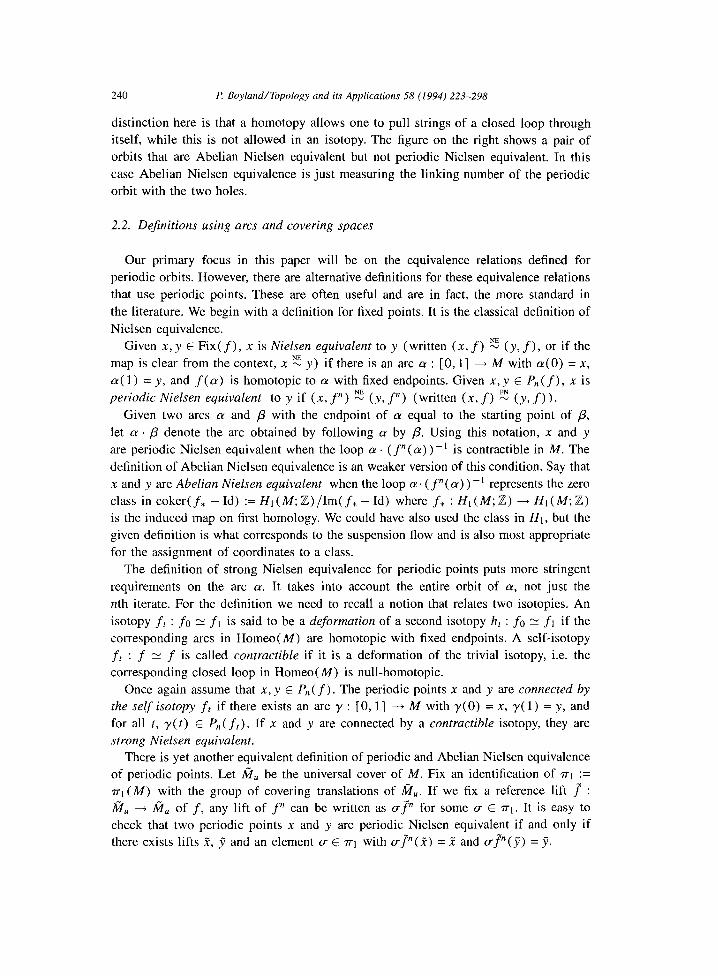
240 P. Boyland/Topology and ifs Applications 58 (1994) 223-298
distinction here is that a homotopy allows one to pull strings of a closed loop through
itself, while this is not allowed in an isotopy. The figure on the right shows a pair of
orbits that are Abelian Nielsen equivalent but not periodic Nielsen equivalent. In this
case Abelian Nielsen equivalence is just measuring the linking number of the periodic
orbit with the two holes.
2.2. Dejinitions using arcs and covering spaces
Our primary focus in this paper will be on the equivalence relations defined for
periodic orbits. However, there are alternative definitions for these equivalence relations
that use periodic points. These are often useful and are in fact, the more standard in
the literature. We begin with a definition for fixed points. It is the classical definition of
Nielsen equivalence.
Given x, y E Fix(f), x is Nielsen equivalent to y (written (x, f) z (y. f), or if the
map is clear from the context, x E y) if there is an arc (Y : [0, l] + M with a(O) = X,
a( 1) = y, and f( cu) is homotopic to CY with fixed endpoints. Given X, y E P,(f), x is
periodic Nielsen equivalent to y if (x, f”) 2 (y, f”) (written (x, f) E (y, f)).
Given two arcs CY and /3 with the endpoint of cy equal to the starting point of p,
let CY . /3 denote the arc obtained by following (Y by /3. Using this notation, n and y
are periodic Nielsen equivalent when the loop cy . ( f”(a) ) -’ is contractible in M. The
definition of Abelian Nielsen equivalence is an weaker version of this condition. Say that
x and y are Abelian Nielsen equivalent when the loop (Y. (f”( (Y) ) -’ represents the zero
class in coker( f* - Id) := Ht (M; Z) /Im( f* - Id) where f* : HI (M; Z) -+ H1 (M; Z)
is the induced map on first homology. We could have also used the class in HI, but the
given definition is what corresponds to the suspension flow and is also most appropriate
for the assignment of coordinates to a class.
The definition of strong Nielsen equivalence for periodic points puts more stringent
requirements on the arc cy. It takes into account the entire orbit of a, not just the
nth iterate. For the definition we need to recall a notion that relates two isotopies. An
isotopy fr : fo rv j-1 is said to be a deformation of a second isotopy hr : fo 5 fl if the
corresponding arcs in Homeo(M) are homotopic with fixed endpoints. A self-isotopy
fr : f Y f is called contractible if it is a deformation of the trivial isotopy, i.e. the
corresponding closed loop in Homeo( M) is null-homotopic.
Once again assume that X, y E P,(f) The periodic points x and y are connected by
the self isotopy fr if there exists an arc y : [ 0, 1 ] -,Mwithy(O)=x,y(l)=y,and
for all t, y(t) E P,,( ft). If x and y are connected by a contractible isotopy, they are
strong Nielsen equivalent.
There is yet another equivalent definition of periodic and Abelian Nielsen equivalence
of periodic points. Let fiu be the universal cover of M. Fix an identification of ~1 :=
~1 (M) with the group of covering translations of M,. If we fix a reference lift f :
fi, + fi, of f, any lift of f” can be written as gp for some CT E n-1. It is easy to
check that two periodic points x and y are periodic Nielsen equivalent if and only if
there exists lifts .Z-, y” and an element CT E ~1 with (TV = .? and a?(y) = 7.

P Boyland/Topology and its Applications 58 (1994) 223-298 241
The definition of Abelian Nielsen equivalence makes use of the cover with deck group
coker( f* - Id). Denote this covering space &r (the subscript “F” stands for Fried cf.
[ 501). The space fin is the largest Abelian cover to which f lifts, and all lifts commute
with the deck transformations. One can check that two periodic points n and y are
Abelian Nielsen equivalent if and only if there exists lifts W, J to fin and an element
u E coker( f+ - Id) with gp( 3) = f and VP(~) = jj.
In comparing the definitions giving here with those elsewhere in the literature it is
important to note that we have always defined equivalence relations just on periodic
points of the same period. This is not always standard.
2.3. Connecting the de$nitions
At this point we have described the equivalence relations on periodic orbits using the
suspension and on periodic points using arcs and covering spaces. The next proposition
connects these definitions.
Proposition 2.1. Two periodic orbits are equivalent in a given sense if and only if there
are points from each of the orbits that are equivalent in the same sense. For example,
0(x, f) E o(y, f) ifand only if there exists integers k and j with fk(x) E fj(y).
For periodic Nielsen equivalence this result is proved in [ 8 1 ] (cf. [ 551) . The Abelian
Nielsen equivalence result is implicit in [50,54,34]. Part of the strong Nielsen equiv-
alence result is in [4], while the rest is (not completely trivial) exercise in smooth
approximations and differential topology.
2.4. Remarks
It is clear from the definitions that use the suspension flow that o(x) z o(y) implies
o(x) 2 o(y) implies o(x) 2 o(y). This means that a periodic Nielsen class is com-
posed of a disjoint collection of strong Nielsen classes and an Abelian Nielsen class
is composed of a disjoint collection of periodic Nielsen classes. For fixed points there
is no difference between the notions of strong and periodic Nielsen equivalence ( [ 78,
Theorem 2.13 ] ) .
The definition of strong Nielsen equivalence using arcs required a contractible self-
isotopy. This is necessary to insure that the definition is equivalent to that given in the
suspension flow. The basic idea is that the self-isotopy induces a self-homeomorphism
of the suspension manifold. The isotopy is required to be contractible so that this
homeomorphism is isotopic to the identity and thus does not alter isotopy classes.
From another point of view, one would certainly like strong Nielsen equivalence to
imply periodic Nielsen equivalence for periodic points. Using the definition of periodic
Nielsen equivalence in the universal cover, this follows from the fact that a contractible
self-isotopy always lifts to self-isotopy in the universal cover. In the case of primary
interest here (M is a compact orientable surface with negative Euler characteristic) all

242 I? Boyland/Topology and its Applications 58 (1994) 223-298
self-isotopies are contractible (cf. [ 37, p. 221) . However, the definition of strong Nielsen
equivalence is applicable in other situations so the condition is explicitly mentioned here.
Strong Nielsen equivalence of periodic orbits requires that the closed orbits be iso-
topic in the three-dimensional suspension manifold. This indicates the close connection
of strong Nielsen equivalence with knot theory in dimension 3 (cf. [ 121). It also in-
dicates that the distinction between strong and periodic Nielsen equivalence vanishes in
dimensions bigger than two. In this case the suspension manifolds will be dimension 4
or greater and in these dimensions simple closed curves are homotopic if and only if
they are isotopic.
2.5. Examples
For degree-one maps of the circle (Section 1.3)) the suspension manifold is the torus.
Since closed curves in T2 are isotopic if and only if they are homotopic if and only if
they are homologous, all three equivalence relations are the same. Two periodic orbits
are equivalent precisely when they have the same period and rotation number. For circle
homeomorphisms the period is determined by the rotation number.
For the doubling map on the circle, Hd, coker( (Hd) * -Id) = Z/Z, so Abelian Nielsen
equivalence only measures the period here. To study the periodic Nielsen classes note
that all lifts to the universal cover of H; have the form x H 2k~ + N. Such a map can
have at most one fixed point and so all fixed points of iY2 are in different Nielsen classes.
Thus all periodic orbits of Hd are in different periodic Nielsen equivalence classes.
For the linear toral automorphisms Hf and HA from Section 1.5 the analysis of
periodic Nielsen equivalence is similar. All the lifts of all the iterates will have at most
one fixed point with the exception being Hfk = Id. This means that all the period 2
points of Hf are periodic Nielsen equivalent. Note that any fixed point of Hf is Nielsen
equivalent as a fixed point of Hf’ to any of the period 2 points and to any other fixed
point. However, the fixed points are not periodic Nielsen equivalent to each other or
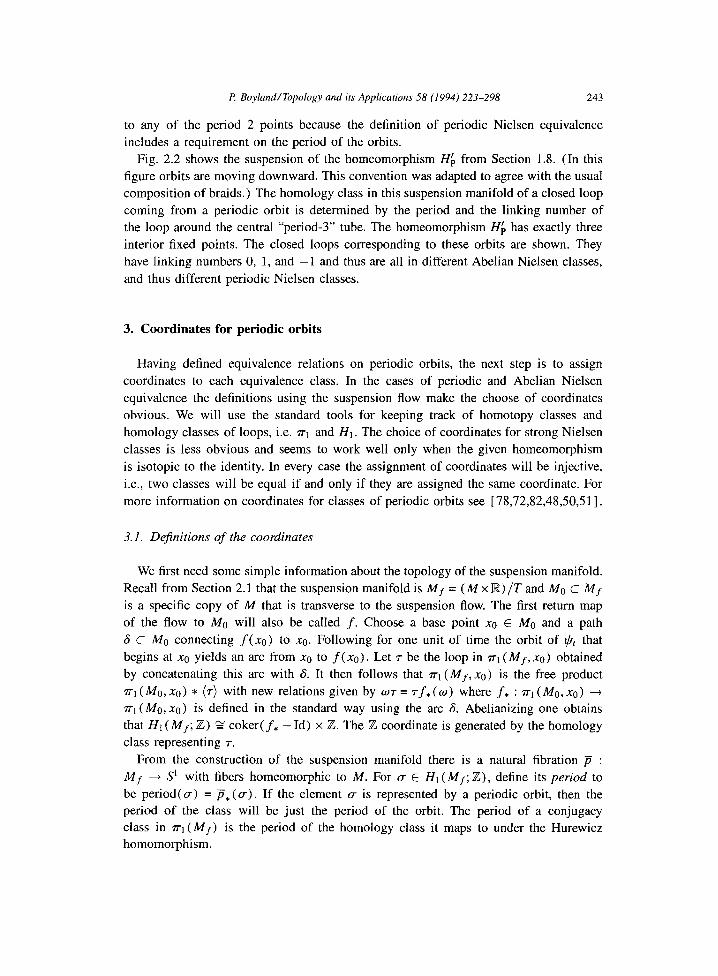
Fig. 2.2. The suspension of H6.
P. BoylandlTopology and its Applications 58 (1994) 223-298 243
to any of the period 2 points because the definition of periodic Nielsen equivalence
includes a requirement on the period of the orbits.
Fig. 2.2 shows the suspension of the homeomorphism Hfi from Section 1.8. (In this
figure orbits are moving downward. This convention was adapted to agree with the usual
composition of braids.) The homology class in this suspension manifold of a closed loop
coming from a periodic orbit is determined by the period and the linking number of
the loop around the central “period-3” tube. The homeomorphism Hf, has exactly three
interior fixed points. The closed loops corresponding to these orbits are shown. They
have linking numbers 0, 1, and -1 and thus are all in different Abelian Nielsen classes,
and thus different periodic Nielsen classes.
3. Coordinates for periodic orbits
Having defined equivalence relations on periodic orbits, the next step is to assign
coordinates to each equivalence class. In the cases of periodic and Abelian Nielsen
equivalence the definitions using the suspension flow make the choose of coordinates
obvious. We will use the standard tools for keeping track of homotopy classes and
homology classes of loops, i.e. ~1 and HI. The choice of coordinates for strong Nielsen
classes is less obvious and seems to work well only when the given homeomorphism
is isotopic to the identity. In every case the assignment of coordinates will be injective,
i.e., two classes will be equal if and only if they are assigned the same coordinate. For
more information on coordinates for classes of periodic orbits see [ 78,72,82,48,50,51].
3.1. Dejinitions of the coordinates
We first need some simple information about the topology of the suspension manifold.
Recall from Section 2.1 that the suspension manifold is Mf = (M x R) /T and Ma c MJ
is a specific copy of M that is transverse to the suspension flow. The first return map
of the flow to MO will also be called f. Choose a base point x0 E MO and a path
6 c MO connecting f(xc) to xc. Following for one unit of time the orbit of I,$ that
begins at xc yields an arc from x0 to f( xc). Let T be the loop in n-1 (Mf, xc) obtained
by concatenating this arc with S. It then follows that ~-1 (Mf, x0) is the free product
~1 (Mu, x0) * (r) with new relations given by wr = rf, (w) where f* : n-1 (MO, x0) + n-1 (MO, x0) is defined in the standard way using the arc 6. Abelianizing one obtains
that HI (Mf; Z) 2 coker( f* - Id) x Z. The Z coordinate is generated by the homology
class representing 7.
From the construction of the suspension manifold there is a natural fibration p :
Mf + S’ with fibers homeomorphic to M. For (T E H1 (Mf; Z), define its period to
be period(a) = P,(U). If the element c is represented by a periodic orbit, then the
period of the class will be just the period of the orbit. The period of a conjugacy
class in n-1 (Mf) is the period of the homology class it maps to under the Hurewicz
homomorphism.

244 I? Boyland/Topology and its Applications 58 (1994) 223-298
Given x E P,,(f) its Abelian Nielsen type, denoted ant( x, f) is the homology class
of yx in the suspension Mf. Writing Hi (Mf; Z) as above, the last coordinate of an
Abelian Nielsen type keeps track of the period of periodic orbit. The periodic Nielsen
type of the periodic orbit, denoted pnt(x, f), is the conjugacy class in ~1 (Mf) that
represents the free homotopy class of yx.
We are focusing here on assigning coordinates to periodic orbits. One can also, in
the case of Abelian and periodic Nielsen equivalence, assign coordinates to a periodic
point. These coordinates keep track of which lifts in the appropriate cover fix a lift of the
point. For periodic Nielsen equivalence these coordinates are called lifting classes and f-
twisted conjugacy classes (see [ 781) . Different period n-periodic points from the same
periodic orbit will have different coordinates if they are not Nielsen equivalent under f”.
The coordinate assigned to the Abelian Nielsen class of periodic point is the projection
of its Abelian Nielsen type to coker( f* - Id). This coordinate will be the same for all
points on the same orbit as they are always Abelian Nielsen equivalent. This coordinate
may be viewed as the element w E coker( f* - Id) for which f”( 2) = w? in fin.
There only seem to be reasonable algebraic coordinates for strong Nielsen classes
when f is isotopic to the identity. The strong Nielsen type of the orbit will be essentially
the isotopy class of f rel the orbit, but we eventually will compare periodic orbit from
different maps so we need to transport this data over to a common model. For each
n E N, let X, E Int( M) be a set consisting of n distinct points. Given a periodic orbit,
o(x,f), of period n, pick a homeomorphism h : (M,o(x, f)) + (M,X,) isotopic to
the identity. Now let the strong Nielsen type of the orbit, denoted snt(x, f), be the
conjugacy class of [ h-‘fh] in MCG( M rel X,), where [ .] represents the isotopy class.
Now one can show that 0(x, f) E o(y, f) if and only snt(x, f) = snt(y, f).
3.2. The collection of equivalence classes for a map
We now have a method of assigning coordinates to the periodic orbits of a home-
omorphism. It is natural to collect all these coordinates together and associate them
with the homeomorphism. This collection of coordinates encodes a great deal of in-
formation about the dynamics of the homeomorphism and its size gives some measure
of the dynamical complexity. We let snt( f) = {snt(x, f) : 0(x, f) is a periodic orbit},
pnt(f) = {pnt(x,f) : o(x,f) is a periodic orbit}, and ant(f) = {ant(x,f) : o(x,f>
is a periodic orbit}.
The methods for computing these objects will be discussed in later sections. The
analog of the set ant(f) that takes into account non-periodic orbits is called the rotation
set and will be discussed in Section 11.
3.3. Growth rate of equivalence classes
The growth rate of the number of distinct equivalence classes of period n-orbits as
n 4 0~) gives a measure of the size of the set of all classes and so measures the
complexity of the dynamics.
P Boyland/Topology and ifs Applications 58 (1994) 223-298 245
For each n E N, let pnt(f, n) be the number of distinct period n-periodic Nielsen
classes for f and pnt”( f) = growth(pnt( f, n) ), where growth is the exponential
growth rate defined in Section 1.2. Note that for each n, pnt(f, n) is always finite.
This is one reason the growth rate of period Nielsen classes is studied instead of that
of Fix(fn). The following theorem is proved like Theorem 2.7 from [ 821 (see also
[ 731). The result here is only slightly different as we are counting only least period II
classes and are counting non-essential classes (the notion of an essential class will be
defined in the next section).
Theorem 3.1. Given a homeomorphism f : M 4 M, then htop(f) 3 pm”(f).
The theorem says that the topological entropy is larger than the exponential growth
rate of the number of distinct periodic Nielsen classes of period n. This implies a similar
theorem for Abelian Nielsen classes.
3.4. Examples
As noted in Section 1.5, for circle endomorphisms the suspension manifold is T2
which has integer homology iZ2. All three equivalence relations in this case measure the
same thing. The type of a periodic orbit will be a pair (m, n) where n is the period
and m/n is the rotation number. The set of all the rotation numbers of the map G, from
Section 1.3 was computed in that section.
As also noted in Section 1.5, the Abelian Nielsen type of a periodic orbit of the angle
doubling map, Hd, is just the period. The periodic Nielsen type is more interesting. We
first consider the task of understanding the fixed points of Hz. Since n-1 (S’ ) is abelian,
the set of free homotopy classes in the suspension that have period II is in one-to-one
correspondence with coker( (Hz) * - Id) = Z/( 2” - 1 )Z = &,_i. Each of these free
homotopy classes is represented by some closed loop corresponding to a fixed point
of H;. (Many of these loops correspond to periodic orbits with periods that divide n.
These loops are traversed multiple times.) In fact, the fixed points of Hz are exactly the
points in the circle with angles
{
1 2 2” - 2 o,-- - 2” _ 1’ 2” _ 1 ‘. . ’ 2” _ 1
I
which is a subgroup of S’ that is isomorphic to &_i.
Now to understand the periodic Nielsen types of orbits we must consider how the
period k orbits are accounted for among the fixed points of H; when k divides m.
This amounts to understanding how Z2’-’ is sent inside Z*“-’ by the natural map. In
addition, we want a description of the conjugacy class of the orbit not just the individual
fixed points of iterates. This is an entertaining exercise in elementary number theory
that we leave to the reader.
Since n-1 (T*) is Abelian the situation is similar but the number theory is much more
complicated (cf. [ 1171). The free homotopy classes in the suspension of period II
246 R Boyland/Topology and its Applications 58 (1994) 223-298
will be in one-to-one correspondence with coker( f: - Id) (here we have once again
allowed multiples of lower period classes). For a hyperbolic toral automorphism like
HA from Section 1.5, each of these classes will be represented by an orbit. For example,
coker( (Hi) * - Id) 2 Zs, where we have used the fact that the action of HA on first
homology is given by the matrix CA. Now the Lefschetz formula yields that the sum of
the indices of fixed points of Hi is 1 - trace( (Hi),) + 1 = -5. Each fixed point of
Hi will have index - 1 (see the derivative formula in Section 4.2)) and thus there must
be 5 fixed points. They are all in different Nielsen classes and so each of the period-2
classes in the suspension is represented by a closed loop coming from a fixed point of
Hi. A similar analysis shows that the number of period-n periodic Nielsen classes will
grow like the trace of Ci, thus pnP ( HA) = log( At ) - 0.962424.
For the finite-order map Hf, the cokernel is & @ & whose four elements correspond
to the four fixed points of Hf. Since there are only finitely many periodic orbits, the
growth rate pnP is zero.
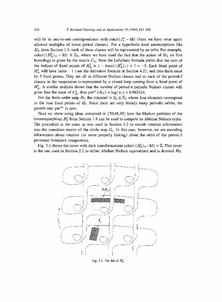
Next we show using ideas contained in [50,48,39] how the Markov partition of the
homeomorphism HL from Section 1.8 can be used to compute its Abelian Nielsen types.
The procedure is the same as was used in Section 1.2 to encode rotation information
into the transition matrix of the circle map G,. In this case, however, we are encoding
information about rotation (or more properly linking) about the orbit of the period-3
permuted boundary components.
Fig. 3.1 shows the cover with deck transformations coker( (Hb) * -Id) = Z. This cover
is the one used in Section 2.2 to define Abelian Nielsen equivalence and is denoted A?i;l~.
Fig. 3.1. The lift of Hk.

l? BoylandITopology and its Applications 58 (1994) 223-298 247
Fig. 3.2. The action of Hb on an arc
The idea is to lift the Markov partition to fin and then compute the transition matrix
there when we act by a lift of HL. For simplicity we pick a lift that fixes the back edge
of fir and call this lift 8.
The figure shows the action on the rectangle 1?t. This behavior can be computed by
studying the behavior of the arc labeled LY in Fig. 3.2. We can think of the covering
space as being constructed by cutting along all the dotted lines shown in Fig. 3.2. The
fact that HL( cr) crosses a cut line means that in the lift, the image of the rectangle I?’
moves upward a deck transformation and intersects another lift of the same rectangle.
We record this information by putting a e in the (1,1) place in the new transition
matrix. By computing the action on all boxes we obtain the matrix
Note that since fi commutes with the deck transformations, it does not matter what lift
of a given rectangle we consider.
The matrix K encodes all the information about the behavior of the lifts of orbits
from the main piece of the recurrent set. This means that it contains all the information
we need to compute Abelian Nielsen types. For example, since trace( K2) = 1 + !-’ + 2[-’ + 2e + e2, the second iterate of Hb has fixed points with linking number 0, -2,
- 1, 1, and 2. Note that just the - 1 and 1 represent period-2 orbits, the others are the
second iterates of fixed points (see Fig. 2.2). Thus the period-2 Abelian Nielsen types
are (- 1,2) and ( 1,2). In Section 11 we will remark on how the minimal loops of the
Markov partition can be used to compute the rotation set of Hb. We have adapted here the point of view of the covering space in computing the
Abelian Nielsen types. This point of view is developed in [ 501. We could also have
adopted the point of view of the suspension flow as in [39,49,48]. In this case the
matrix K is the linking matrix of the suspension flow. It records how the boxes in the
Markov partition link with the period three tube in Fig. 2.2 as they traverse once around
the suspension manifold under the suspension Bow.
248 P. BoylandlTopology and its Applications 58 (1994) 223-298
4. Isotopy stability of equivalence classes of periodic orbits
In this section we discuss conditions on the equivalence class of a periodic orbit which
ensure that it persists under isotopy, i.e. it is present in the appropriate sense in any
isotopic map. To make this somewhat more precise, recall that the equivalence relations
on periodic orbits have been defined using the suspension flow. Isotopic maps have
homeomorphic suspension manifolds, and so it makes sense to compare equivalence
classes of isotopic maps. A given type of periodic orbit is isotopically stable if its type
is always present among the types of the isotopic map.
The persistence of fixed points, or more generally periodic points, is the subject of
Nielsen fixed point theory. This theory applies in a much broader framework than is
discussed here (see, for example, [78,99]).
4.1. Correspondence of equivalence classes in isotopic maps
Given an isotopy ft : fo N fl, let F : Mfo 4 Mf, be the induced homeomor-
phism of the suspension manifolds. Say snc(xa, fa) corresponds under the isotopy
fr : fo N fl to snc(xt , fl) if F(y,,) is isotopic to yx, in Mf,. Similarly, two periodic
Nielsen classes correspond if these two closed curves are homotopic, and two Abelian
Nielsen classes correspond if they are homologous. These correspondences have been
defined using particular elements of the classes, but it is clearly independent of these
choices.
It would be natural to say that two classes correspond if they have the same type or
coordinate. This requires a consistent way of assigning coordinates to periodic orbits for
all elements in an isotopy class. An isotopy induces a homeomorphism of the suspension
manifold, and this gives a way of identifying coordinates for isotopic maps. However, if
the class contains a non-contractible self-isotopy, this will induce a homeomorphism of
the suspension manifold that is not isotopic to the identity. As such it will identify the
coordinates for classes that are not equal. This difficulty can be avoided by restricting
to the case in which there are only contractible isotopies, e.g. when the manifold has
negative Euler characteristic (see Section 2.4), or MCG(D’ rel A, aD2).
We leave it to the reader to check that following give the appropriate notions of
correspondence under isotopy for periodic points using arcs and covering spaces. If
ff : fo 21 fl and xi E P,, (fi), then pnc( no, fa) corresponds to pnc(xt , fl) under this
isotopy if there exists u E ~1 and lifts to the universal cover with mfi(Zi) = .Fi where
fl : fo N ?I with ff an equivariant isotopy. Equivalently, the periodic points correspond
under the isotopy if there is an arc y : [0, 11 - M with y(0) = x0, y( 1) = xi, and the
curve fr ( y( t) ) is homotopic to y(t) with fixed endpoints. The correspondence under
isotopy for Abelian Nielsen equivalence classes is similar, but one uses the cover tin,
or requires that the loop y-’ . fy(y(t)) vanish in coker(ft, -Id) g coker(f2, -Id).
The definition of correspondence for strong Nielsen classes is similar to equivalence
relation in that case. The periodic points x0 and x1 are connected by the isotopy fr if
there exists an arc y : [0, l] -+ M with y(0) = x0, y(1) = xl, and for all t, y(t) E

P Boyland/Topology and its Applications 58 (1994) 223-298 249
P,( ft>. If (x0, fa) and (xi, fl ) are connected by an isotopy that is a deformation of
fr, then their strong Nielsen classes correspond under fr.
4.2. Uncollapsible and essential classes
Sufficient conditions for the isotopy stability of an equivalence class of periodic
orbits have two requirements. The first requirement is a non-zero fixed point index for
an iterate of the map. This detects the fact that an iterate has a fixed point. The second
requirement is something called the uncollapsibility of the class, which implies that the
fixed point is for the correct iterate. In terms of the bifurcation theory of dynamical
systems, isotopy stability means that in a one parameter family of homeomorphisms the
class of the periodic orbit cannot disappear. The uncollapsible condition insures that the
class cannot disappear in a period dividing bifurcation. The index condition insures that
the class cannot disappear via saddle node. The equivalence relation on the periodic
orbits enters here because periodic orbits in different equivalence classes cannot interact
in the suspension in a parameterized family.
The definition of collapsible is first given for periodic Nielsen equivalence. The
periodic orbit 0(x, f) of period n is collapsible if there exists a closed loop /3 in Mf
so that yX is freely homotopic to pk for some 1 < k < n, where pk means the loop
obtained by going k times around the loop p (see Fig. 4.1) . A period Nielsen class is
collapsible if any (and thus all) of its elements is collapsible. In terms of coordinates,
a periodic Nielsen type a is collapsible if there is a element b E n-1 (Mf) so that a is
conjugate to bk for some 0 < k < n. Of necessity, the period of a is k times that of b.
For surface homeomorphisms, the next lemma shows that the element b in the last
paragraph is always represented by an orbit of f. We need the notion of one periodic
point collapsing to another. If x and y are periodic points with (x, f”) z (y, f”) but
n = pert x, f) > per(y, f), x is said to collapse to y. One periodic orbit is collapsible
to another if periodic points from each orbit do.
f
Fig. 4.1. A collapsible periodic orbit with an orbit to which it collapses.
250 f? BoylandITopology and its Applications 58 (1994) 223-298
What is termed “uncollapsible” here is what was called “irreducible” in [ 78, p. 651.
That terminology is not used to avoid confusion with the terminology “reducible maps”
used in Thurston-Nielsen theory. The lemma contains the conditions that could be taken
as the definition of collapsible using a covering space. The lemma is proved in [ 231.
Lemma 4.1. If f : M ----f M is an orientation-preserving homeomorphism of a compact
orientable 2-manifold and x E P,,(f), then following are equivalent:
(a) pnc( x, f) is collapsible;
(b) pnt( x, f) is collapsible;
(c) There exist integers k and m with 1 < k < n and n = mk, an element (T E ~1,
and a lifts 2 and f to the universal cover so that 5 is a periodic point with
period m under cfk;
(d) There exists a periodic point y so that x collapses to y.
A strong Nielsen class is said to be collapsible if its periodic Nielsen class is col-
lapsible. An Abelian Nielsen class is collapsible if its Abelian Nielsen type is divisible
in Ht (Mf; Z), i.e. it is the non-trivial multiple of another class. Note that a collapsible
Abelian Nielsen class may not contain a collapsible periodic Nielsen class. Also note
that if an uncollapsible periodic Nielsen class for fo corresponds under an isotopy to
a class for fl, then the class for fl is also uncollapsible. Similar comment holds for
strong and Abelian Nielsen classes.
The second ingredient of isotopy stability results is the fixed point index. This index
assigns an integer, Z( X, f ), to any set X of fixed points of f that is closed in M and
open in Fix(f) . For a smooth map an isolated fixed point at the origin has index equal to
sgn( det( Id -D f (0) ) when the determinant is non-zero. The index has very strong local
homotopy invariance properties. This invariance is globalized to equivalence classes to
obtain isotopy stability results. An account of the fixed point index is given in [40] and
[ 781, and an in-depth account in [ 271.
Lemma 4.2. An uncollapsible period n-periodic, -strong, or -Abelian Nielsen class is
open in Fix(f”) and closed in M.
The index of a period-n class of periodic orbits is the index of the class as fixed
points of f”. A periodic, strong, or Abelian Nielsen class for which the index is defined
and is non-zero is called essential.
4.3. Zsotopy stability of equivalence classes
The strong Nielsen class snc(xa, fo) of a xa E P,, (fo) is isotopy stable if whenever
ft : fo N fl there is a xt E P,,( fl) with snc(xt, fl) corresponding to snc(xa, fo) under
the isotopy. We further require (which will always be satisfied) that Z (snc( no, fo) , fo) = Z (snc( x1, f 1) , f ;) . Isotopy stability is defined similarly for periodic and Abelian Nielsen
equivalence.
P Boyland/Topology and its Applications 58 (1994) 223-298 251
Theorem 4.3. (a) If a strong, periodic or Abelian Nielsen class is uncollapsible and
essential then it is isotopy stable.
(b) A strong or periodic Nielsen class is isotopy stable if and only if it is uncollapsi-
ble and essential.
The proof of (a) for periodic Nielsen classes is in [ 781 and for strong Nielsen classes
in [ 611 extending [4]. The result for Abelian Nielsen classes follows from the twisted
Lefschetz theorem in [ 501 and [ 341. Part (b) is proved in [ 231 using a refinement of
the Thurston-Nielsen canonical form that will be discussed in Section 7.
4.4. Remarks
Some of the results in this section are special to surfaces while others hold in more
general circumstances. Lemma 4.2, Theorem 4.3(a) and the equivalence of (a), (b)
and (c) in Lemma 4.1 hold in general. The inclusion of condition (d) in Lemma 4.1
is special to surfaces as is Theorem 4.3(b).
Theorem 4.3 (b) allows one to attach a list of isotopy stable data to an isotopy class.
This list includes the coordinates of all the isotopy stability classes as well as their index.
This list of data will be exactly the dynamics of the minimal representative discussed in
the next section. There are a number of algebraic methods for computing this data, see
[ 78,82,72,35,50]. A very effective geometric technique is given in Section 10.
Theorem 4.3(b) does not contain necessary and sufficient conditions for the isotopy
stability of an Abelian Nielsen class. Such conditions do not exist because, for example,
a Abelian Nielsen class can have zero index and still be isotopy stable if it contains an
uncollapsible and essential strong Nielsen class. This could happen when the indexes
of all the strong Nielsen classes in the Abelian class add up to zero. This type of
cancellation is very common on surfaces. This remark also explains why there is no
analog for Abelian Nielsen equivalence of Theorem 5.1 from the next section.
If x E P,,(f) and all the points in 0(x, f) are in different Nielsen classes as fixed
points of f”, then the period Nielsen class of x is uncollapsible. This is the necessary
condition given for isotopy stability in [4].
4.5. Examples
A simple example shows why the uncollapsible condition is required to define the
index. Let H : D2 -+ D2 be rotation of the unit disk by 180 degrees about the origin. The
set of period 2 points is the disk minus the origin which is not compact. Of course, the set
Fix( H2) is compact, but we are studying sets of periodic orbits using their least period.
There is no homotopy stability for periodic orbits of degree-one maps of the circle.
Every such map is homotopic to a homeomorphism that has no periodic orbits, namely,
rigid rotation by a irrational angle. Similarly, in the identity class on the torus and
annulus, there are no isotopy stable periodic orbits. If the Euler characteristic of a
surface is non-zero, then the isotopy stable classes in the identity isotopy class consist

252 P. BoylandITopology and its Applications 58 (1994) 223-298
of a single fixed point class whose index is the Euler characteristic (as it must be by
the Lefschetz formula).
For the hyperbolic toral automorphism HA, we saw in Section 2.5 that for any IZ, all
the fixed points of Hi are in different Nielsen classes. By the last remark in Section 4.4,
this implies that all the periodic orbits of HA are uncollapsible. Using the derivative
formula for the index from Section 4.2 one has that all the periodic orbits have index
-1 and are therefore isotopy stable. This implies the same result for all the interior
periodic orbit of the map HK of Section 1.8.
For the finite-order toral automorphism Hf, all the fixed points are in different Nielsen
classes and have index 1 and so are isotopy stable. On the other hand, all the period 2
points are collapsible, because for example, they lift to period orbits for Cf in the cover
(Lemma 4.1(c)).
The situation of periodic orbits on the boundary often requires a little more effort.
As an example on the torus, let H, = Hf o HA, and H$ is obtained by blowing up the
fixed point of H,. This fixed point is a so-called flip saddle, and so there will be a pair
of period-2 orbits for Hk on the boundary. Call one of these orbits o( z ) . Now despite
the fact that the two elements of O(Z) are Nielsen equivalent under (Hk)*, the orbit is
still uncollapsible. If it were collapsible, then by Lemma 4.1 (d), there would have to
be a fixed point of HL that it was Nielsen equivalent to it under (Hk)*. By blowing the
boundary circle back down this would imply that two fixed points of Hz are Nielsen
equivalent, which does not happen. The orbit also has non-zero index, so it is isotopy
stable.
5. Dynamically minimal representatives
In this section we discuss the dynamically simplest map in an isotopy class. There
are, of course, a variety of ways to make precise the notion of simplest. The notion
used here relies on the various types of equivalence defined for periodic orbits. The next
section deals with more general orbits.
5.1. Existence of the minimal representative
The theorem asserts the existence of a minimal representative with respect to periodic
and strong Nielsen equivalence in the category of orientation-preserving homeomor-
phisms of compact orientable surfaces. The corresponding theorem for Nielsen fixed
point classes is outlined in [ 771 and [ 741 and given in full detail in [ 831.
Theorem 5.1. Each orientation-preserving homeomorphisms of a compact, orientable
2-manifold is isotopic to a homeomorphism @ so that each class in snt(@) and pnt(@)
is uncollapsible, essential and contains exactly one periodic orbit.
The theorem is proved in [23] and utilizes a refinement of the Thurston-Nielsen
I? Boyland/Topology and its Applications 58 (1994) 223-298 253
canonical representative in the isotopy class (see Section 7.5). The actual construction
of this refinement is somewhat complicated, but some examples are given below.
5.2. Remarks
Theorem 4.3(b) is an easy corollary of Theorem 5.1. The conditions on the strong
and periodic Nielsen classes for the dynamically minimal representative insure that the
map has only equivalence classes of periodic orbits that are isotopy stable. Further,
these classes are represented in the simplest possible way, i.e. by a single periodic orbit
that carries all the index of the class. In general, there can be many non-conjugate
dynamically minimal representatives in an isotopy class.
It is important to note there is no theorem of this type even for fixed point theories for
certain homotopy classes of maps on surfaces that are not homeomorphisms ( [ 79,801).
5.3. Examples
For circle endomorphisms one could consider the stability of periodic orbits rel a
finite set. In this case, the map G, from Section 1.2 would be the dynamically minimal
representative rel the finite set o(c, G,). It is somehow more economical to conjugate
G, to get a map whose slope has a constant absolute value equal to the exponential
of the topological entropy. The angle doubling map on S’ is another example of the
one-dimensional analog of a dynamically minimal representative. All its periodic orbits
are uncollapsible and essential and there is just one in each class. For similar reasons
the hyperbolic toral automorphism HA is also dynamically minimal in its class.
On the other hand, the finite-order toral automorphism Hf is not dynamically minimal
as it has collapsible period-2 orbits. To get a minimal representative, first pass to the
quotient as a branched cover T2 --) T2/Hf. As noted in Section 1.8, this is a two-fold
branch cover over the sphere with four branch points. Now pick a flow on the sphere
that has just these four points as fixed points of non-zero index and no other fixed points.
Call g the time one map of this flow and lift it to G : T2 ---f T2 that is isotopic to Hf. The set of periodic orbits of G consists of exactly four fixed points that have non-zero
index, and all of these fixed points are in different Nielsen classes. This means that G
is a dynamically minimal representative.
This general technique works to find the minimal representative in any finite-order
class on a surface (cf. [23]). This example also illustrates the difference in a dynami-
cally minimal representative for fixed points and that for periodic orbits. Since Hf = id,
the minimal representative in the class of Hf contains no fixed points. This is not the
iterate of any minimal representative in the class of Hf, and so no single map can be
dynamically minimal with respect to fixed points in the isotopy classes of all iterates.
The other main technique needed to get a minimal representative on surfaces involves
the boundary. Let Ha be derived from the hyperbolic toral automorphism HA by blowing
up the fixed point. This will result in four fixed points on the boundary that are in the
same Nielsen class (see Fig. 1.6). Now this class is essential and uncollapsible but it
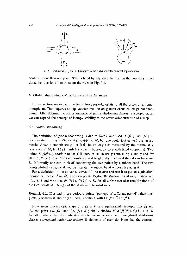
254 I? Boyland/Topology and its Applications 58 (1994) 223-298
Fig. 5.1. Adjusting Ha on the boundary to get a dynamically minimal representative
contains more than one point. This is fixed by adjusting the map on the boundary to get
dynamics that look like those on the right in Fig. 5.1.
6. Global shadowing and isotopy stability for maps
In this section we expand the focus from periodic orbits to all the orbits of a home-
omorphism. This requires an equivalence relation on general orbits called global shad-
owing. After defining the correspondence of global shadowing classes in isotopic maps,
we can expand the concept of isotopy stability to the entire orbit structure of a map.
6.1. Global shadowing
The definition of global shadowing is due to Katok, and used in [ 671 and [ 681. It
is convenient to use a Riemannian metric on M, but one could just as well use an arc
metric. Given a smooth arc p, let e(p) be its length as measured by the metric. If y
is any arc in M, let L(y) = inf{e(p) : j? is homotopic to y with fixed endpoints}. Two
points K-globally shadow under f if there exists an arc y connecting x and y and for
all i, L( f(r) > < K. The two points are said to globally shadow if they do so for some
K. Informally one can think of connecting the two points by a rubber band. The two
points globally shadow if you can iterate the rubber band without breaking it.
For a definition in the universal cover, lift the metric and use it to get an equivariant
topological metric d on fi, The two points K-globally shadow if and only if there are
lifts, f”, 5 and 3 so that d( F(X), p( 9) ) < K, for all i. One can also roughly think of
the two points as tracing out the same infinite word in ~1.
Remark 6.1. If x and y are periodic points (perhaps of different period), then they
globally shadow if and only if there is some k with (x, fk) E (y, fk).
Now given two isotopic maps fr : fo 21 fl and equivariantly isotopic lifts ?a and
ft, the pairs (xo,fo) and (xt,ft) K-globally shadow if d(fi(Zc),fi(Rt)) < K
for all i, where the tilde indicates lifts to the universal cover. Two global shadowing
classes correspond under the isotopy if elements of each do. Note that the constant
P Boyland/Topology and its Applications 58 (1994) 223-298 255
K may depend on choice of representatives from the two classes. In terms of arcs,
the pairs correspond if there exists an arc y connecting xa and xt so that for all i,
Uf;(y(t))) < K.
6.2. Isotopy stability for homeomorphisms
We now define a notion of persistence that includes all the dynamics of a map. A
map 4 : M + M is weak isotopy stable if whenever g = 4 there exists a compact,
g-invariant set Y and a continuous surjection LY : Y + M that is homotopic to the identity
so that cr o gly = 4 o LY. If for all such g, one can choose Y = M, then 4 is strong isotopy
stable.
As noted in Section 1.1, the dynamics of an extension are always at least as compli-
cated as those of the factor. This means that all the dynamics of $ persist in a precise
sense. The name isotopy stability points out an analogy to structural stability. Small
perturbations of structurally stable maps are conjugate. Isotopy stability allows large
perturbations, but only gives a semi-conjugacy.
The next theorem extracts the main elements from a result in [ 671. It shows the close
connection between global shadowing and the isotopy stability of maps.
Theorem 6.2. Assume that 4 : M -+ M satisJies:
(a) Each global shadowing class of 4 contains exactly one element.
(b) The periodic orbits of C$ are dense in M and all have non-zero index.
(c) If g y q4, there is a constant K(g) so that (x, 4) globally shadows (y, g) if
and only if it does so with constant K(g).
Then Y = {(y, g) : (y, g) globally shadows some (x. $) } is a compact g-invariant set
and the map LY : Y --) M that sends y to the point x it globally shadows gives a
semiconjugacy of (I: g) with (M, 4).
Here is the idea of the proof. The set Y is obviously g-invariant and it is compact by
(c). Condition (a) shows that the map LY is well defined, while (c) shows that it is
continuous. By (a) and Remark 6.1, all the periodic orbits of q5 are uncollapsible. They
are essential by (b) and thus are isotopy stable. The image of a therefore includes a
dense set in M and since Y is compact, the image is M. Note that nothing in the proof
is special to surfaces.
6.3. Remarks
Theorem 6.2 gives conditions for the persistence of a global shadowing class when
it occurs in a certain type of map. It seems natural to seek the analogs for global
shadowing classes of the results of the previous section for classes of periodic orbit. It
is not clear whether there is an analog of Theorem 4.3 for global shadowing classes,
i.e. conditions on a class that insure that it persists under isotopy. The assignment of
coordinates also seems problematic.
256 I? BoylandITopology and its Applications 58 (1994) 223-298
An outline of the history of dynamical stability under homotopy or isotopy is given in
[ 121. The Lefschetz formula can be viewed in this light as well some of Nielsen’s work
on surfaces. Franks showed that Anosov diffeomorphisms on tori of any dimension are
strong isotopy stable [ 381. There is an analogous property called homotopy stability that
Shub showed holds for expanding maps [ 1131. Handel [67] and Fathi [ 361 showed
isotopy stability (in fact homotopy stability) for pseudoAnosov maps on surfaces (see
Theorem 7.4).
6.4. Examples
For annulus homeomorphisms, points that globally shadow will have the same rotation
number, but the converse is not true. The rotation number measures linear rates; two
points can drift apart under iteration at a sublinear rate and still have the same rotation
number, but they will not globally shadow.
Each pair of points in the torus globally shadow under the finite-order map Hf. This
is obvious because the map lifts to a rigid rotation by 180” in the plane. This illustrates
Remark 6.1. Note that there is not a uniform bound for points that shadow in the lift.
We now show that a hyperbolic toral automorphism satisfies the conditions of Theorem
6.2. For concreteness we focus on the map HA. The method of argument is taken from
[ 671 and directly generalizes to show that pseudoAnosov maps are weak isotopy stable
(Theorem 7.4(b)). We have remarked in Section 4.5 that HA satisfies condition (b) of
Theorem 6.2.
Recall from Section 1.5 that a lift of HA to the plane is a linear map given by a
matrix CA that has unstable eigenvector ut associated to the eigenvalue h > 1, and
stable eigenvector 02 associated to the eigenvalue l/h. Any z E R2 can be written as
z = ztut + ~2~2. Now for two points z, w E Iw2, let &(z, w) = Izt - wt 1 and Js( z, w) =
122 - ~21. These will define equivariant pseudo-metrics on R2 that will satisfy
d;,(C*(~),C*(j9) = A&(&j%
&(C,‘(Z),C,-‘(9)) = hJs(a,g). (*)
We can get an equivariant metric that is equivalent to the standard one by defining
2 = &, + zs. If .? and j are a positive distance apart, then their separation as measured
by 2 grows exponentially under forward or backward iteration (or both). This shows
that HA satisfies condition (a) of Theorem 6.2.
To show that (c) is also satisfied, fix a f N HA and fix a lift f” equivariantly isotopic
to CA (in a slight abuse of notation we use the notation CA to represent the linear map
coming from the matrix CA). Now let
and K = 2( R + 1) /( h - 1). Using the triangle equality and property (*) we have
Ju(C~(Z),f(y)) 3 ,\di,(R,jj) -R. Thus if &(Z,B) 3 K/2, then &u(C~(R),.f(j;)) 3
1 +&(Z,g), and so &(C;;(?),p(j)) ---f cc as n --f co.
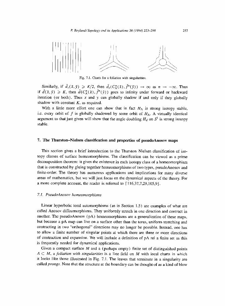
P Boyland/Topology and its Applications 58 (1994) 223-298 257
Fig. 7.1. Charts for a foliation with singularities.
Similarly, if J$(Z.,y”) > K/2, then ~~(C~(Z),~(J)) + 00 as n --+ -co. Thus
if d( 2, jj) 3 K, then d”( CL(i), J”( 7) ) goes to infinity under forward or backward
iteration (or both). Thus x and y can globally shadow if and only if they globally
shadow with constant K, as required.
With a little more effort one can show that in fact HA is strong isotopy stable,
i.e. every orbit of f is globally shadowed by some orbit of HA. A virtually identical
argument to that just given will show that the angle doubling Hd on S’ is strong isotopy
stable.
7. The Thurston-Nielsen classification and properties of pseudoAnosov maps
This section gives a brief introduction to the Thurston-Nielsen classification of iso-
topy classes of surface homeomorphisms. The classification can be viewed as a prime
decomposition theorem: it gives the existence in each isotopy class of a homeomorphism
that is constructed by gluing together homeomorphisms of two types, pseudoAnosov and
finite-order. The theory has numerous applications and implications for many diverse
areas of mathematics, but we will just focus on the dynamical aspects of the theory. For
a more complete account, the reader is referred to [ 116,37,7,29,105,9].
7.1. PseudoAnosov homeomorphisms
Linear hyperbolic toral automorphisms (as in Section 1.5) are examples of what are
called Anosov diffeomorphisms. They uniformly stretch in one direction and contract in
another. The pseudoAnosov (PA) homeomorphisms are a generalization of these maps,
but because a pA map can live on a surface other than the torus, uniform stretching and
contracting in two “orthogonal” directions may no longer be possible. Instead, one has
to allow a finite number of singular points at which there are three or more directions
of contraction and expansion. We will include a definition of pA rel a finite set as this
is frequently needed for dynamical applications.
Given a compact surface M and a (perhaps empty) finite set of distinguished points
A c M, a foliation with singularities is a line field on M with local charts in which
it looks like those illustrated in Fig. 7.1. The leaves that terminate in a singularity are
called prongs. Note that the structure at the boundary can be thought of as a kind of blow
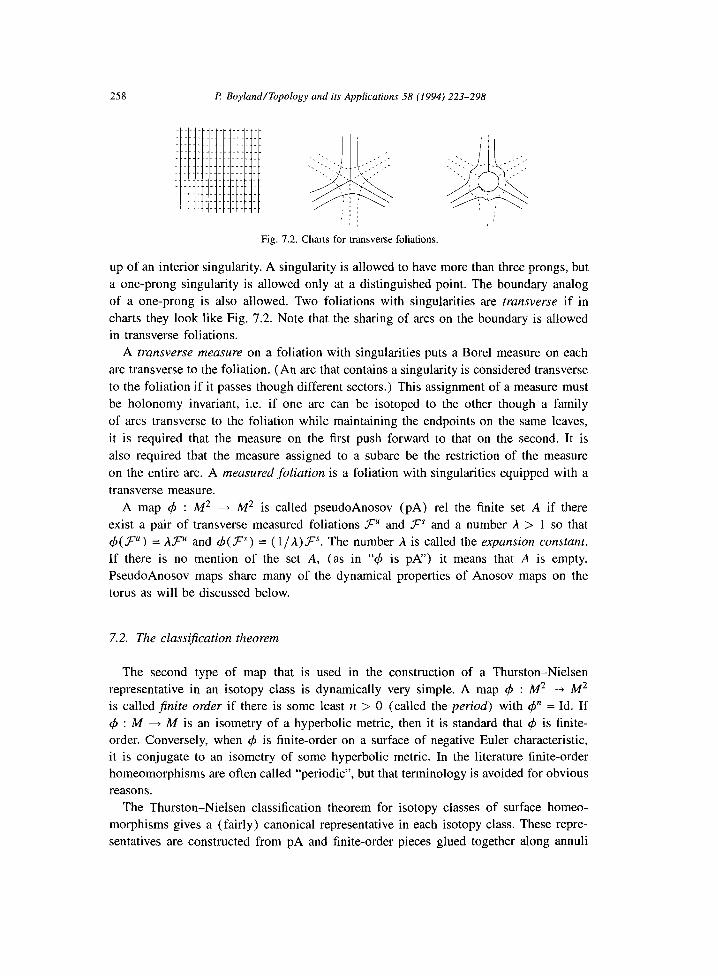
258 P: Boyland/Topology and its Applications 58 (1994) 223-298
. ..__._. _. . . .._ _..
r----.-------------
Fig. 7.2. Charts for transverse foliations.
up of an interior singularity. A singularity is allowed to have more than three prongs, but
a one-prong singularity is allowed only at a distinguished point. The boundary analog
of a one-prong is also allowed. Two foliations with singularities are transverse if in
charts they look like Fig. 7.2. Note that the sharing of arcs on the boundary is allowed
in transverse foliations.
A transverse measure on a foliation with singularities puts a Bore1 measure on each
arc transverse to the foliation. (An arc that contains a singularity is considered transverse
to the foliation if it passes though different sectors.) This assignment of a measure must
be holonomy invariant, i.e. if one arc can be isotoped to the other though a family
of arcs transverse to the foliation while maintaining the endpoints on the same leaves,
it is required that the measure on the first push forward to that on the second. It is
also required that the measure assigned to a subarc be the restriction of the measure
on the entire arc. A measured foliation is a foliation with singularities equipped with a
transverse measure.
A map 4 : M2 + M2 is called pseudoAnosov (PA) rel the finite set A if there
exist a pair of transverse measured foliations FU and FS and a number A > 1 so that
$(.?=““) = UK and d(F‘“) = ( l/A)FS. The number A is called the expansion constant.
If there is no mention of the set A, (as in “#J is PA”) it means that A is empty.
PseudoAnosov maps share many of the dynamical properties of Anosov maps on the
torus as will be discussed below.
7.2. The classification theorem
The second type of map that is used in the construction of a Thurston-Nielsen
representative in an isotopy class is dynamically very simple. A map 4 : M2 -+ M2
is called finite order if there is some least n > 0 (called the period) with @’ = Id. If
$J : A4 --f M is an isometry of a hyperbolic metric, then it is standard that 4 is finite-
order. Conversely, when 4 is finite-order on a surface of negative Euler characteristic,
it is conjugate to an isometry of some hyperbolic metric. In the literature finite-order
homeomorphisms are often called “periodic”, but that terminology is avoided for obvious
reasons.
The Thurston-Nielsen classification theorem for isotopy classes of surface homeo-
morphisms gives a (fairly) canonical representative in each isotopy class. These repre-
sentatives are constructed from pA and finite-order pieces glued together along annuli
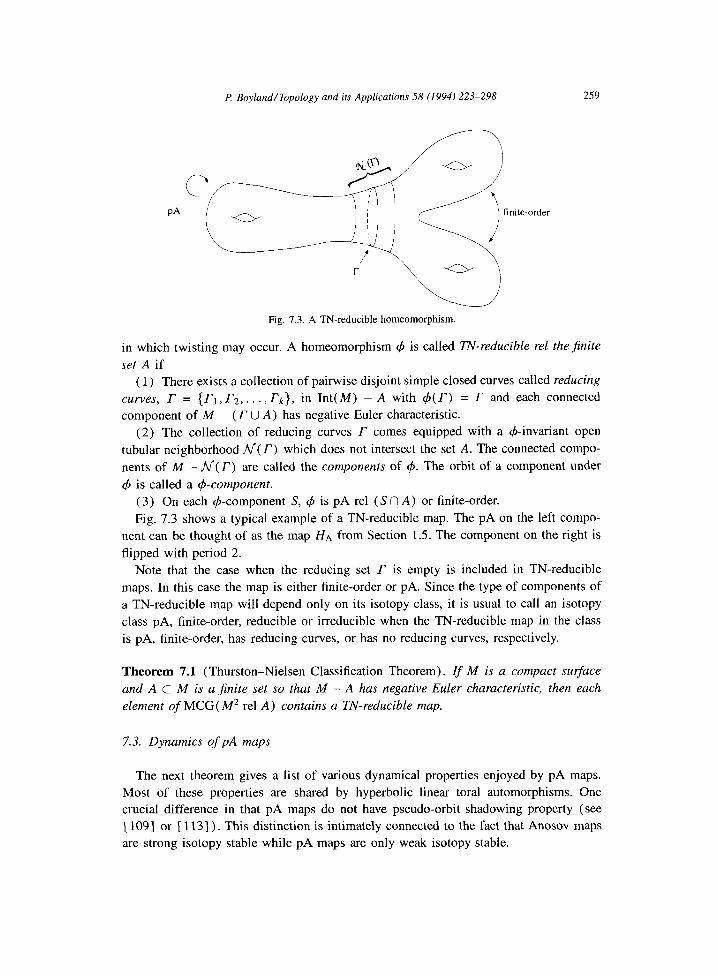
P Boyland/Topology and its Applications 58 (1994) 223-298 259
PA
Fig. 7.3. A TN-reducible homeomorphism.
in which twisting may occur. A homeomorphism 4 is called TN-reducible rel the$nite
set A if
(1) There exists a collection of pairwise disjoint simple closed curves called reducing
curves, r = (rl, r2,. . . , rk), in Int(M) - A with 4(r) = r and each connected
component of M - (r U A) has negative Euler characteristic.
(2) The collection of reducing curves r comes equipped with a &invariant open
tubular neighborhood ni( r) which does not intersect the set A. The connected compo-
nents of M - N(r) are called the components of 4. The orbit of a component under
4 is called a &component.
(3) On each $-component S, 4 is pA rel (S f? A) or finite-order.
Fig. 7.3 shows a typical example of a TN-reducible map. The pA on the left compo-
nent can be thought of as the map HA from Section 1.5. The component on the right is
flipped with period 2.
Note that the case when the reducing set r is empty is included in TN-reducible
maps. In this case the map is either finite-order or pA. Since the type of components of
a TN-reducible map will depend only on its isotopy class, it is usual to call an isotopy
class pA, finite-order, reducible or irreducible when the TN-reducible map in the class
is pA, finite-order, has reducing curves, or has no reducing curves, respectively.
Theorem 7.1 (Thurston-Nielsen Classification Theorem). Zf M is a compact surface
and A c M is a finite set so that M - A has negative Euler characteristic, then each
element of MCG( M2 rel A) contains a TN-reducible map.
7.3. Dynamics of pA maps
The next theorem gives a list of various dynamical properties enjoyed by pA maps.
Most of these properties are shared by hyperbolic linear toral automorphisms. One
crucial difference in that pA maps do not have pseudo-orbit shadowing property (see
[ 1091 or [ 1131) . This distinction is intimately connected to the fact that Anosov maps
are strong isotopy stable while pA maps are only weak isotopy stable.
260 P Boyland/Topology and its Applications 58 (1994) 223-298
Recall that the exponential growth rate snt”(f) was defined in Section 3.3. Given
a finite f-invariant set A, snP( f rel A) is the exponential growth rate of the periodic
Nielsen classes of f in the punctured manifold M - A.
Theorem 7.2. If q5 : M + M is pA rel the (perhaps empty) finite set A and has
expansion constant A then
(a) 4 has a Markov partition with irreducible transition matrix B, and thus (M, C#J)
is a factor of (A,, a).
(b) The collection of &periodic orbits is dense in M and there exist points x with
0(x, 4) dense in M*.
(c) The topological entropy of 4 is htop( 4) = log(A) = pnt”( f rel A).
(d) Every leaf of .P and F’” is dense in M.
(e) The measure on M obtained from the transverse measures is the unique measure
of maximal entropy for 4 and is ergodic. After a continuous change of coordinates one
may assume that this measure is Lebesgue measure.
Sometimes it is useful to think of a pA map as being constructed from its Markov
partition. One thinks of gluing rectangles together to get the surface. The pA map will
act linearly on the rectangles. If the surface is not the torus, there will have to be points
(the singularities) where three or more rectangles have to come together. Every pA map
is conjugate to a smooth ( [ 581) or real analytic map ( [ 921). There is also a surprising
topological characterization of pA maps (when the set A is empty): a map is pA on a
closed surface if and only if it is expansive ( [ 9 1,7 11) .
7.4. Isotopy stability and entropy
It should be clear that there is a very sharp dichotomy between the dynamics of
pA and finite-order maps. This dichotomy extends to the isotopy stability properties. A
finite-order map has only finitely many isotopy stable classes of periodic orbits while a
pA map has infinitely many. In fact, a pA map is essentially (except for some boundary
periodic orbits) a dynamically minimal map.
We first discuss the situation with finite-order maps. A periodic orbit of a finite-order
homeomorphism that has the same period as the homeomorphism is called regular;
any orbit with lesser period is called a branch periodic orbit. Since only orientation-
preserving finite-order maps are considered here, the set of branch periodic orbits is
always finite. The next proposition follows easily after lifting the given finite-order map
to a finite-order isometry of the hyperbolic disk (cf. Lemma 1.1 of [ 231) .
Proposition 7.3. Assume 4 : M + M is$nite-order and M has negative Euler charac-
teristic.
(a) Each regular periodic orbit is periodic Nielsen equivalent to every other regular
periodic point, each branch periodic orbit is not periodic Nielsen equivalent to any
other branch periodic orbit, and each regular periodic orbit is collapsible to any branch
P: Boyland/Topology and its Applications 58 (1994) 223-298 261
periodic orbit.
(b) If 4 has no branch periodic orbit, then all periodic orbits are in a single periodic
Nielsen class and this class is isotopy stable. When 4 has branch periodic orbits, each
of these periodic orbits is alone in an isotopy stable periodic Nielsen class and there
are no other isotopy stable classes.
Part (a) of the next theorem follows from Thurston’s original work (cf. [ 111) . Part
(b) was proved by Handel [ 671 and Fathi [ 361. The main ingredients in Handel’s proof
were abstracted in Theorem 6.2. The application of that theorem to pA maps is virtually
identical to that for hyperbolic toral automorphisms given in Section 6.4. In the case of
pA maps one uses the transverse measures to get the pseudo-metrics used in equation
(*) from Section 6.4.
Theorem 7.4. Assume 4 : M -+ M is pA and M is closed.
(a) Each x E P,,( 4) has non-zero index and is alone in its Y-Nielsen class. Thus
its strong and periodic Nielsen classes are uncollapsible and essential and therefore
isotopically stable.
(b) The homeomorphism q5 is weak isotopy stable.
The situation is somewhat more technical when the surface has boundary. In that
case there can be periodic orbits on the same boundary component that are Nielsen
equivalent as fixed points of an iterate. Nonetheless their periodic Nielsen class will
still be uncollapsible and essential and thus isotopy stable (as with the map H,,, from
Section 4.5). The situation for isotopy stability of the pA map when there is boundary
is discussed at the end of [ 671 and in [ 231. The next result is a corollary of the weak
isotopy stability of pA maps.
Corollary 7.5. Assume q5 : M + M is pA rel A and has expansion constant h.
(a) Zfg E 4 rel A, then h,,,(g) b sntOO(grel A) 2 htop(q5) = log(A) > 0.
(b) If Q N 4 rel A and ~,4 is also pA rel A, then ti and 4 are conjugate.
Part (a) of the next theorem follows from a result of Smillie. He showed that when
a homeomorphism isotopic to a pA map has a fixed point that is not Nielsen equivalent
to a fixed point of the pA map, then it has strictly larger entropy. Part (b) is proved in
[ 681. Note that by Remark 6.1, part (a) is a consequence of part (b) .
Theorem 7.6. Assume that 4 : M + M is pA, M is closed, and g N 4. (a) If pnt( g) - pnt ( 4) contains a uncollapsible element, then htop (g) > htop ( 4).
(b) If there is a orbit o( y, g) that does not globally shadow any 0(x, 4), then
pnt”(g) > pnt”(4) and hop(g) > htop(4).
Again, the analogous result with boundary or rel a finite set is more technical but is
understood. Note that any element in pnt(g) - pnt( 4) must of necessity be inessential.
This is because the pA map contains all the isotopy stable periodic Nielsen classes

262 P: Boyland/Topology and its Applications 58 (1994) 223-298
and by Theorem 4.3(b), these are precisely the classes that uncollapsible and essential.
Note also by the construction of the map cy in Theorem 6.2, the hypothesis in (b) is
equivalent to saying that g is not semiconjugate to 4. Thus the contrapositive of (b) is:
if h,,(g) = htop( 4)) then g is semiconjugate to 4.
The hypothesis of Theorem 7.6(a) can never be satisfied by a hyperbolic toral au-
tomorphism. For these maps, every potential periodic Nielsen type contains a periodic
orbit already (see Section 3.4). Any isotopic map is in fact semi-conjugate, i.e. they are
strong isotopy stable.
7.5. Reducible isotopy classes and TN-condensed homeomorphisms
In a certain sense, most isotopy classes are not pA or finite-order, they are reducible
and so we need to understand the isotopy stable dynamics in reducible classes. Although
the TN-reducible map defined in Section 7.2 is sometimes called the Thurston-Nielsen
canonical representative in its class, the definition does not specify the behavior on the
tubular neighborhood of the reducing curve. The TN-reducible maps as defined are also
not dynamically minimal; they may possess collapsible periodic Nielsen classes as well
as having multiple periodic orbits in certain classes.
A refinement of a TN-reducible map is used to get the dynamical minimal represen-
tative of Theorem 5.1. The basic idea is to get a minimal number of periodic orbits in a
pA component by adjusting the boundary as in Fig. 5.1 and in a finite-order component
via the technique applied to Hf in Section 5.3. There is also an adjustment that must
be done to coalesce periodic points in different components that are periodic Nielsen
equivalent. The result of this refinement is called a TN-condensed map. The analog of
weak isotopy stability for TN-condensed maps is somewhat technical to state. Basically,
the dynamics of any pA component persist up to semiconjugacy (as in Theorem 7.4(b) )
and the isotopy stability periodic orbits of the finite-order component (specified in The-
orem 7.3(b)) also persist. The technicalities arise for orbits on the boundaries of pA
components and in the interaction of orbits from different components (see [23] ).
We will content ourselves with the following result that summarizes some of the
properties of TN-condensed homeomorphisms. Note that since a TN-condensed home-
omorphism is constructed from a TN-reducible one, there will be a TN-condensed
homeomorphism in each isotopy class.
Theorem 7.7. Let @ : M --) M be a TN-condensed homeomorphism rel the$nite set A
and g N @ rel A.
(a) htOp(g) 3 snP(g rel A) 2 htop(@) = log(&), where A, is the largest expansion
constant of any pA component of CD. If @ has no pA components, it has zero topological
entropy.
(b) All the strong Nielsen classes of periodic orbits of CD are isotopy stable rel A.
(c) Zf 0(x, @) is contained in the interior of a pA component of @, then there is a
o( y, g) that globally shadows it.
F! Boyland/Topology and its Applications 58 (1994) 223-298 263
7.6. Examples
The map Hf from Section 1.5 is an example of a finite-order order map. Although it
is not defined on a surface of negative Euler characteristic, Proposition 7.4 still describes
its isotopy stable dynamics. As we saw in Section 5.3, the four branch points are fixed
points and all the period 2 points are collapsible to these fixed points. Indeed, there is
a map isotopic to Hf that has these four fixed points as its only periodic orbits.
The simplest pA maps are the Anosov maps on the torus. In this case the pair of
invariant foliations are the projection of foliations of the plane by lines parallel to the
eigenvectors. The expansion constant is just the largest eigenvalue of the matrix and the
transverse measures come from using the eigenvectors as coordinates for the plane as in
Section 6.4.
Other examples of pA maps can be obtained by blowing up periodic orbits (as in
Section 1.6) or else projecting to the disk (as in Section 1.8). The map HK is pA rel the
period three orbit that comes from the branch points. The map Hf, is pA on the genus
zero surface with four boundary components. It is an entertaining exercise to draw the
invariant foliations of these maps by projecting the irrational wrappings on the torus.
8. Hidden pA maps
In this section we give dynamical applications of the theory described thus far. The
main strategy in these applications is to use the Thurston-Nielsen theory to determine
the isotopy stable dynamics rel a periodic orbit for a given homeomorphism f ( [ 161).
These dynamics will be present in any element in this relative isotopy class, in partic-
ular, they must be present in the homeomorphism f. If the TN-reducible map in this
class contains a pA component, then the isotopy stable dynamics in the class are very
complicated, and this provides a lower bound for the dynamical complexity of f. Some-
what surprisingly, one can often determine the structure of the TN-reducible map from
very limited combinatorial data about the periodic orbit. The first results that used this
strategy concerned orientation-reversing homeomorphisms and were due to Blanchard
and Franks [ 131 and Handel [ 651.
8.1. Hidden pA components
Given a homeomorphism f : M + M and a finite f-invariant set A, f is said to
have a hidden pA component rel A if the TN-reducible map in the isotopy class of f
rel A has a pA component. When there exists at least one such set A, f is said to
have a hidden pA component. If the TN-reducible map is pA, then f is hidden pA rel
A. The next proposition is a consequence of Theorem 7,7(a). It is one way of giving
precise expression to the fact that homeomorphisms with hidden pA components must
have complicated dynamics.
264 F1 BoylundITopology and its Applications 58 (1994) 223-298
Proposition 8.1. If a homeomorphism f : M --+ M has a hidden pA component rel A,
then htop ( f) > pnt”( f rel A) > 0.
Theorem 7.7(c) provides another way of looking at maps f which have hidden pA
components. The presence of a hidden pA component implies the existence of a f-
invariant set Y that is semiconjugate to a pA map. This means that f restricted to this
set is dynamically very complicated.
8.2. Homeomorphisms of the disk and annulus
For genus zero surfaces, the Jordan curve theorem coupled with Theorem 8.3 often
make it fairly simple to determine whether a given periodic orbit implies a hidden pA
component. The next theorem is basically folklore and was contained in [ 171.
Theorem 8.2. Let f : D2 + D2 be an orientation preserving homeomorphism of the
disk with a periodic orbit o( x, f) whose period is the prime number q. If there is an
arc a connecting x and fk(x), and the arc f‘J(a) is not homotopic to a rel 0(x, f), then f is hidden pA rel o( x, f).
The main observation needed in the proof is that the isotopy class rel the orbit must
be irreducible. Any reducing curve for the isotopy class rel 0(x, f) would have to
enclose at least 2 points from the orbit, but not all q points. The reducing curves must
be permuted which would show that q has non-trivial factors. The conditions on the arc
cy insure that the class rel the orbit is not finite-order, and so it must be pA.
The next theorem of Brouwer [ 261, Kerekjarto [ 871, and Eilenberg [ 331, allows for
a characterization of finite-order maps on genus zero surfaces. Define R,,l, : D2 + D2
in polar coordinates as R,l,( r, 8) = (r, 8 +p/q) . The analogous homeomorphism of the
annulus will also be called R,l,.
Theorem 8.3. If 4 is an orientation-preserving homeomorphism of the disk or annulus
that satis$es @ = id, then C/J is topologically conjugate to RPiq for some 0 < p < q.
The next result concerns homeomorphisms of the annulus and is somewhat analogous
to Theorem 8.2. In this case a condition on the rotation number of the orbit (or its
Abelian Nielsen type) implies that the isotopy class rel the orbit is irreducible ( [ 211) .
The hypothesis that eliminates the finite-order possibility is nicest in the case of mono-
tone twist maps of the annulus. An homeomorphism f of the annulus A that is isotopic
to the identity is called monotone twist if for the lift to the universal cover fl : A + A,
the image of each vertical arc is a graph (see Fig. 8.1). If f is differentiable, then it
is (right) monotone twist if aJ’t /ay > 0. A periodic orbit 0(x, f) is called monotone
if f is order preserving on p-’ (o( x, f) ), where p : d 4 IR is the projection. This
means that for z,w E p-‘(0(x, f)), (Z)I 6 (W)I must imply (f(z>)l < (f(w))l, where (Z ) 1 means the first coordinate of z in the strip A. For more information on the
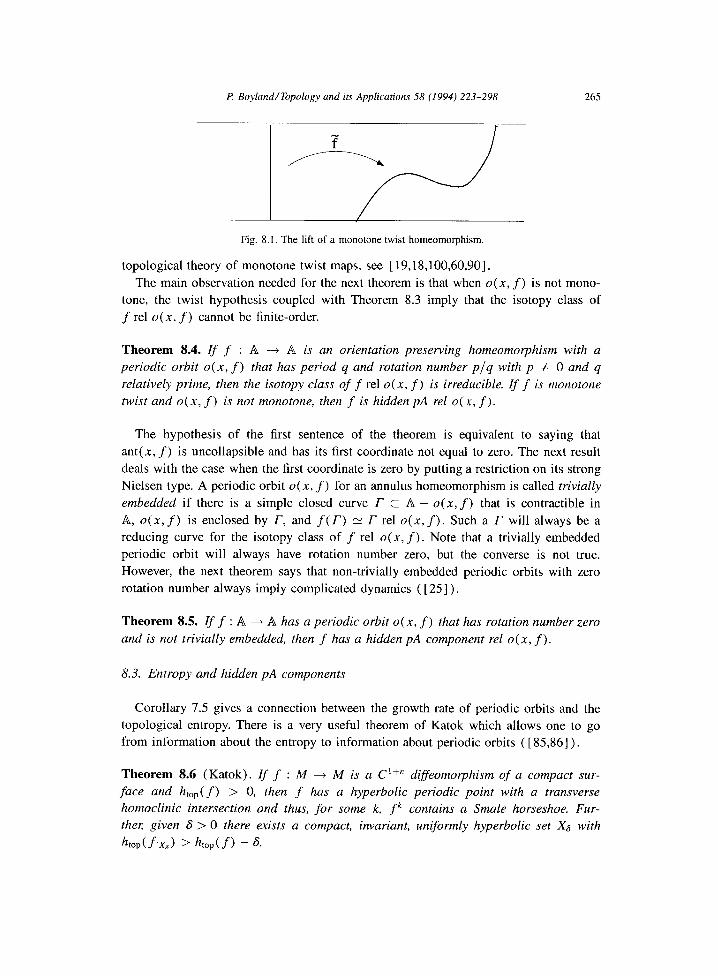
P Boyland/Topology and its Applications 58 (1994) 223-298 265
Fig. 8.1. The lift of a monotone twist homeomorphism.
topological theory of monotone twist maps, see [ 19,18,100,60,90].
The main observation needed for the next theorem is that when 0(x, f) is not mono-
tone, the twist hypothesis coupled with Theorem 8.3 imply that the isotopy class of
f rel 0(x, f) cannot be finite-order.
Theorem 8.4. If f : A ---f A is an orientation preserving homeomorphism with a
periodic orbit o(n, f) that has period q and rotation number p/q with p # 0 and q
relatively prime, then the isotopy class off rel 0(x, f) is irreducible. If f is monotone
twist and 0(x, f) is not monotone, then f is hidden pA rel 0(x, f).
The hypothesis of the first sentence of the theorem is equivalent to saying that
ant( x, f) is uncollapsible and has its first coordinate not equal to zero. The next result
deals with the case when the first coordinate is zero by putting a restriction on its strong
Nielsen type. A periodic orbit o( x, f) for an annulus homeomorphism is called trivially
embedded if there is a simple closed curve r C A - 0(x, f) that is contractible in
A, 0(x, f) is enclosed by r, and f(T) z r rel 0(x, f). Such a r will always be a
reducing curve for the isotopy class of f rel 0(x, f). Note that a trivially embedded
periodic orbit will always have rotation number zero, but the converse is not true.
However, the next theorem says that non-trivially embedded periodic orbits with zero
rotation number always imply complicated dynamics ( [ 251) .
Theorem 8.5. If f : A 4 A has a periodic orbit 0(x, f) that has rotation number zero
and is not trivially embedded, then f has a hidden pA component rel o( x, f).
8.3. Entropy and hidden pA components
Corollary 7.5 gives a connection between the growth rate of periodic orbits and the
topological entropy. There is a very useful theorem of Katok which allows one to go
from information about the entropy to information about periodic orbits ( [ 85,861).
Theorem 8.6 (Katok). Zf f : M + M is a C ‘+’ diffeomorphism of a compact sur-
face and htop( f) > 0, then f has a hyperbolic periodic point with a transverse
homoclinic intersection and thus, for some k, fk contains a Smale horseshoe. Fur-
ther given 6 > 0 there exists a compact, invariant, uniformly hyperbolic set X8 with
htop(flxJ) > htop(f) - 6.
266 P. Boyland/Topology and its Applications 58 (1994) 223-298
It is important to note that this type of theorem is not true without some differentia-
bility assumption. There is an example due to Rees [ 1081 of a homeomorphism of the
torus that has positive topological entropy and no periodic orbits, in fact, every orbit is
dense in the torus.
When a smooth map has positive topological entropy, Theorem 8.6 gives the existence
of a horseshoe in an iterate. Using a result like Theorem 8.2, one can get a periodic
orbit that implies a hidden pA component. One may also proceed directly as in [ 451.
Corollary 8.7. Zf f : M -+ M is a C ‘+& diffeomorphism of a compact x&ace and
htop( f) > 0, then there is a periodic orbit 0(x, f) so that f has a hidden pA component
rel 0(x, f).
An analog of the second statement of Katok’s theorem is given in Theorem 9.3. It
concerns the approximation of the entropy of f from below by the entropies associated
with the TN-reducible maps of isotopy classes in f rel finite sets.
8.4. Examples
Theorem 8.2 can be applied to the attracting period three orbit in the homeomorphism
HP from Section 1.8. Any arc connecting two elements of the orbit will not be homotopic
to its third iterate rel the orbit, hence the map is hidden pA rel the orbit.
It is not difficult to see that the homeomorphism of the annulus Hs of Section 1.9
can be isotoped to a monotone twist map rel the period five attracting orbit. This orbit
has rotation number 2/5 and is not monotone, and so Hg is hidden pA rel the orbit by
Theorem 8.4.
9. Dynamical order relations
The last section illustrated how combinatorial information on a periodic orbit can be
used to understand the Thurston-Nielsen type rel the orbit, and thus give a lower bound
on the dynamical complexity of the map. These applications do not use the full strength
of the isotopy stability results for the Thurston-Nielsen canonical form. To get more
information out of the theory, one must feed more data in. This section gives one way
of doing this via dynamical order relations.
9.1. Abstract dynamical order relations
The model for dynamical order relations is the theorem of Sharkovski on the periods
of periodic orbits of continuous maps of the interval ([ 112,115]). That theorem is
generalized by essentially using the structure of its conclusion as a definition, and then
exploring the consequences (cf. [ 101,20].
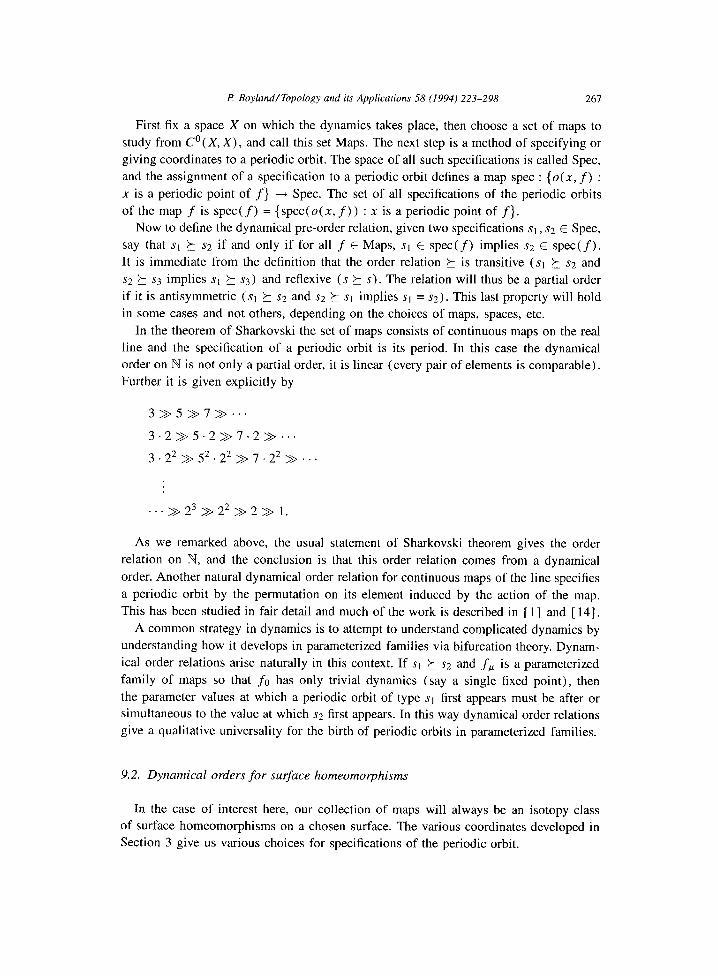
P: Boyland/Topology and its Applications 58 (1994) 223-298 267
First fix a space X on which the dynamics takes place, then choose a set of maps to
study from Co (X, X) , and call this set Maps. The next step is a method of specifying or
giving coordinates to a periodic orbit. The space of all such specifications is called Spec,
and the assignment of a specification to a periodic orbit defines a map spec : {0(.x, f) :
x is a periodic point of f} + Spec. The set of all specifications of the periodic orbits
of the map f is spec( f) = {spec(o(x, f)) : x is a periodic point of f}.
Now to define the dynamical pre-order relation, given two specifications si , s:! E Spec,
say that st k s2 if and only if for all f E Maps, st E spec(f) implies s2 E spec(f).
It is immediate from the definition that the order relation k is transitive ($1 k s2 and
s2 ? ss implies st 5 ~3) and reflexive (s ? s). The relation will thus be a partial order
if it is antisymmetric (st h s2 and s2 k st implies st = ~2). This last property will hold
in some cases and not others, depending on the choices of maps, spaces, etc.
In the theorem of Sharkovski the set of maps consists of continuous maps on the real
line and the specification of a periodic orbit is its period. In this case the dynamical
order on N is not only a partial order, it is linear (every pair of elements is comparable).
Further it is given explicitly by
3 > 5 7 > > . . .
3 2 > 5 .2 >> 7 .2 >> . . .
3 2= 5= 22 >> >> 7 . 22 > . . .
As we remarked above, the usual statement of Sharkovski theorem gives the order
relation on B?, and the conclusion is that this order relation comes from a dynamical
order. Another natural dynamical order relation for continuous maps of the line specifies
a periodic orbit by the permutation on its element induced by the action of the map.
This has been studied in fair detail and much of the work is described in [ 1 ] and [ 141.
A common strategy in dynamics is to attempt to understand complicated dynamics by
understanding how it develops in parameterized families via bifurcation theory. Dynam-
ical order relations arise naturally in this context. If st 5 s2 and fP is a parameterized
family of maps so that fu has only trivial dynamics (say a single fixed point), then
the parameter values at which a periodic orbit of type st first appears must be after or
simultaneous to the value at which s2 first appears. In this way dynamical order relations
give a qualitative universality for the birth of periodic orbits in parameterized families.
9.2. Dynamical orders for surface homeomolphisms
In the case of interest here, our collection of maps will always be an isotopy class
of surface homeomorphisms on a chosen surface. The various coordinates developed in
Section 3 give us various choices for specifications of the periodic orbit.
268 P: Boyland/Topology and its Applications 58 (1994) 223-298
Some of the resulting theories are quite interesting, and a few have been studied
in detail. Some of the theories are trivial. For example, let us restrict to orientation
preserving homeomorphisms of the disk. Since the disk is simply connected, the periodic
and Abelian Nielsen type of an orbit only keep track of the period. Since for each n
there is a homeomorphism of the disk whose periodic orbits have only period n and 1,
in the resulting order relation every number dominates 1 and is unrelated to any other
number. On the other hand, specifying periodic orbits in the disk by their strong Nielsen
type yields a very interesting theory that is the most studied dynamical order relation in
dimension two.
There are also cases in which the pre-order is not antisymmetric. For example, on
the torus let us restrict to homeomorphisms that are isotopic to the linear hyperbolic
automorphism HA from Section 1.5. In Section 4.5 we noted that all the periodic orbits
for this map are isotopically stable and thus are present for every map in the isotopy
class and so the resulting dynamical pre-order will not be antisymmetric. Other theories
seem interesting and tractable, but as yet unstudied, e.g. the order induced on Abelian
Nielsen types for homeomorphisms isotopic to the identity on genus zero surfaces with
more than two boundary components.
The idea of a partial order on periodic orbits is a natural outgrowth of Thurston’s work
on surfaces. Indeed, the idea was in the folklore for some time and was independently
discovered by many people. The idea was inspired in the author ( [ 171) by a paper of
Birman and Williams [ 121.
Let us restrict attention now to homeomorphisms that are isotopic to the identity, but
not fix a surface yet. We study the specification of periodic orbits by their strong Nielsen
type. As noted in Section 3, in the identity isotopy class there is an identification of the
strong Nielsen type with a conjugacy class in a mapping class group. If f : M --t M
is isotopic to the identity and has a periodic orbit 0(x, f) with period n, the strong
Nielsen type of the orbit is essentially the isotopy class of f rel o( x, f > . However, since
we want to compare periodic orbits of different maps, we have to put this data in a
common model of M with a subset X,, where X,, is a set of II points. This involves the
choice of a homeomorphism h : (M, o(x, f) > -+ (M, X,) isotopic to the identity, and
so the strong Nielsen class of the periodic orbits is actually the conjugacy class of the
isotopy class of h f h-' in MCG( M rel X,) . Let us denote the set of all possible strong
Nielsen types of all possible periodic orbits of all homeomorphisms on M isotopic to the
identity as SNT( M, id). The dynamical pre-order relation is denoted (SNT( M, id), 5).
Theorem 9.1. The relation (SNT( M, id), k) is a partial order.
The main ingredient in the proof is a theorem of Brunovsky ( [28] ) which allows
one to find families of diffeomorphisms for which bifurcations of periodic orbits of less
than some fixed period take place at distinct parameter values. This is applied to find
such a nice isotopy from maps with periodic orbits of many different strong Nielsen
types to a simple map, say with its set of periodic orbits consisting of a finite set of
fixed points. Since the periodic orbits of less than a fixed period disappear at distinct

f! Boyland/Topology and its Applications 58 (1994) 223-298 269
parameter values, the strong Nielsen types that are present are also diminishing one by
one. In particular, for any pair of distinct strong Nielsen types, one can find a map that
has one and not the other ( [ 211) .
The partial orders (SNT( M, id), 5) have a very complicated structure and very little
is known about them in general. However, the tools described thus far in the paper give
a clear strategy for their study. Start with a periodic orbit o( x, f) with strong Nielsen
type /3. From the definition of the order relation it follows that the set of elements
dominated by p in (SNT(M, id), k) consists of precisely the isotopy stable strong
Nielsen types in the isotopy class of f rel u(x, f). Further, Theorem 7.7(b) says that
this set is exactly the set of strong Nielsen types of the TN-condensed map in the
isotopy class. So computing in the partial order reduces to computing the dynamics of
the TN-condensed map in an isotopy class. A very effective algorithm for doing this
computation is described in Section 10.
Since a strong Nielsen type is actually a conjugacy class we need to be a little
more precise in specifying what we mean by the TN-condensed map that represents the
strong Nielsen type /?. Given /3 E SNT( M, id), say that @p is a TN-condensed map
that represents /3 if @p has a periodic orbit o(x,@p) with snt(x,@p) = p and @p is a
TN-condensed map in its isotopy class rel 0(x, @p). We talk about a strong Nielsen type
being reducible, irreducible, pA or finite-order when a TN-reducible map that represents
it is of that class. The next theorem formalizes the comments of the previous paragraph.
Theorem 9.2. If j3 E SNT( M, id) and @p is a TN-condensed map that represents /3,
then {y E SNT(M,id) : fi ? y} = snt(@p) = n{snt(f) : f E Homeo(M), f N id, and /3 E snt( f)}.
Most of the progress in understanding the structure of these partial orders has been
made by restricting to suborders or else studying invariants attached to the elements. The
simplest such invariant is the period. A deeper invariant is given by the entropy. Given
p E SNT(M,id), define its topological entropy as h(P) = inf{htop(f) : p E snt(f)}.
By Theorem 7.7(a), h(p) = htop( @pp), where @p is a TN-condensed map that represents
P. Part (a) of the next theorem says that the topological entropy acts as a kind of height
function for the partial order. It is a consequence of Theorem 7.6. Note that pi t p2
trivially implies h(P1) 3 h(&). The content of the theorem is the strict inequality.
Part (b) is a refinement of Corollary 8.7. It can be proved using Theorem 8.6, and then
results of Hall [ 641 on the horseshoe, or else directly as in [ 691.
Theorem 9.3. (a) If p1 and & are distinct pA elements of SNT(M, id) with PI 2 /32,
then h(b) > h(P2). (b) If f : M + M is a C Ifa diffeomorphism that is isotopic to the identity and
htop( f) > 0, then there is a sequence of strong Nielsen types Pn E snt( f) with
h(b) + htop(f 1.

270 P. Boyland/Topology and its Applications 58 (1994) 223-298
9.3. Homeomorphisms of the disk
For homeomorphisms of the disk and annulus the objects in the dynamical order
relation are commonly called braidtypes because of the identification of MCG(D2 rel
n points, JD2) with the braid group on n strings (see Section 1.7). We adhere to this
usage to be consistent with the literature; let snt(x, f) = bt(x, f), bt(f) = snt(f),
and set of all braidtypes of period y1 orbits is BT,, while the set of all braidtypes is
BT = SNT( D2, id). The partial order on braidtypes has been studied in a number of
papers including [ 9.5,47,62,64].
The next result refines Theorem 8.2 by incorporating the characterization of finite-
order maps on genus zero surfaces from Theorem 8.3. It gives another way of checking
whether a periodic orbit implies that the map is hidden pA. It uses the notion of the
exponent sum of a braidtype. If b is an element of the braid group on II strings, its
exponent sum is the sum of the exponents of the generators in a word that represents
the element. For example, the exponent sum of C$CT;’ (~3 is 2. Since the relations in the
group preserve this quantity, it is well-defined. It is also conjugacy invariant, so we can
define the exponent sum of a conjugacy class in the braid group, and thus of a braidtype.
For a braidtype /3, denote its exponent sum as es(P). Let cypj4 be the braidtype of a
periodic orbit of R,lu : D2 + D2. By Theorem 8.3, the only finite-order braidtypes are
the CX,,/~ for various p and q’s. Note that es(a,is) = p(q - 1).
Proposition 9.4. If p E BT has period a prime number q and /3 # cup14 for any p,
then p is PA. In particulal; if es( /I) # p( q - 1) for any p $0 mod q, then p is PA.
If the braidtype does not have prime period one needs much more complete data to
determine its Thurston-Nielsen type (see [98] and [ 61).
As noted above, dynamical order relations are defined using an abstraction of the
conclusion of Sharkovski’s theorem. Ideally, one would like to have the analog of the
other part of that theorem, i.e. a description of the structure of the dynamical order in
terms of the algebraic structure of the set of all specifications. This seems very difficult
in general, but there is one rather special theorem for period three braidtypes that lives
up to this ideal. Recall that the generators of B3 are denoted c$’ and &‘. Part (a) of
the next theorem is from [ 971 and part (b) is due to Handel (personal communication).
Theorem 9.5. (a) Each p E BT3 contains a cyclic word consisting solely of the
generators (~1 and a:’ (and not their inverses). Furthel; p has pA type if and only if
this word has at least one of each of these generators.
(a) (Handel) For PI, & pA braidtypes from BTs, pi h & if and only if the cyclic
word in (~1 and a;’ contained in p2 is obtained from that of PI by deleting generators.
For example, the braidtype represented by the word (ala;‘)* dominates that repre-
sented by the word aiu;’ (see Fig. 9.1). The theorem means that any time you see an
orbit that in the suspension looks like the left of Fig. 9.1, somewhere in the suspension

P Boyland/Topology and its Applications 58 (1994) 223-298 271
Fig. 9.1. The braids (otu;‘)’ and WC;’
there is also an orbit that looks like the right of Fig. 9.1. A little caution must be used
here with the phrase “looks like”. Another way of seeing that one needs a conjugacy in
the definition of the braidtype is that you have to choose a point of view when looking at
the orbit in the suspension. All the different points of view you can take will correspond
to various conjugacies in the braid group.
We should also note that Theorem 9.5 holds if the element of the three braid group
represents the union of a period-two point and fixed point, or the union of three fixed
points. To get this kind of result one needs to extend the notion of a dynamical order
relation from periodic orbits to finite invariant sets.
By Theorem 8.3, the CX~/~‘s are the only irreducible braidtypes with zero entropy. One
can produce reducible braidtypes with zero entropy by using a copy of some aply as each
component. The set of all zero entropy braidtypes is then easily seen to be described by
the collection of lists (pl/ql,p2/q2,. . . , Pk/qk), where pi and qi are relatively prime.
The domination in (BT, ?_) on these elements is generated by dropping the last element
of the list, e.g. (PI /St, m/a,. . . 9Pk+l/qk+l) ? (Pl/41,P2/92,...,Pk/9k) (1114,571). Fig. 9.2 shows a schematic drawing of the tree coming from the partial order on zero
entropy braidtypes.
In the partial order in Sharkovski’s theorem the zero entropy periods are the powers
of two. One would like to understand the approach to the boundary of positive entropy.
POSITIVE ENTROPY
Fig. 9.2. A schematic drawing of the zero entropy braidtype tree.
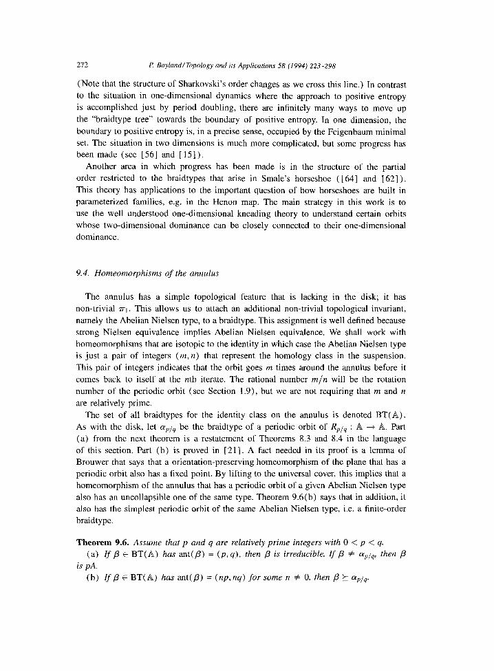
212 I? BoylandlTopology and ifs Applications 58 (1994) 223-298
(Note that the structure of Sharkovski’s order changes as we cross this line.) In contrast
to the situation in one-dimensional dynamics where the approach to positive entropy
is accomplished just by period doubling, there are infinitely many ways to move up
the “braidtype tree” towards the boundary of positive entropy. In one dimension, the
boundary to positive entropy is, in a precise sense, occupied by the Feigenbaum minimal
set. The situation in two dimensions is much more complicated, but some progress has
been made (see [56] and [15]).
Another area in which progress has been made is in the structure of the partial
order restricted to the braidtypes that arise in Smale’s horseshoe ( [64] and [ 621).
This theory has applications to the important question of how horseshoes are built in
parameterized families, e.g. in the Henon map. The main strategy in this work is to
use the well understood one-dimensional kneading theory to understand certain orbits
whose two-dimensional dominance can be closely connected to their one-dimensional
dominance.
9.4. Homeomorphisms of the annulus
The annulus has a simple topological feature that is lacking in the disk; it has
non-trivial ~1. This allows us to attach an additional non-trivial topological invariant,
namely the Abelian Nielsen type, to a braidtype. This assignment is well defined because
strong Nielsen equivalence implies Abelian Nielsen equivalence. We shall work with
homeomorphisms that are isotopic to the identity in which case the Abelian Nielsen type
is just a pair of integers (m, n) that represent the homology class in the suspension.
This pair of integers indicates that the orbit goes m times around the annulus before it
comes back to itself at the nth iterate. The rational number m/n will be the rotation
number of the periodic orbit (see Section 1.9)) but we are not requiring that m and n
are relatively prime.
The set of all braidtypes for the identity class on the annulus is denoted BT(A).
As with the disk, let aplq be the braidtype of a periodic orbit of RPis : A 4 A. Part
(a) from the next theorem is a restatement of Theorems 8.3 and 8.4 in the language
of this section. Part (b) is proved in [ 211. A fact needed in its proof is a lemma of
Brouwer that says that a orientation-preserving homeomorphism of the plane that has a
periodic orbit also has a fixed point. By lifting to the universal cover, this implies that a
homeomorphism of the annulus that has a periodic orbit of a given Abelian Nielsen type
also has an uncollapsible one of the same type. Theorem 9.6(b) says that in addition, it
also has the simplest periodic orbit of the same Abelian Nielsen type, i.e. a finite-order
braidtype.
Theorem 9.6. Assume that p and q are relatively prime integers with 0 < p < q.
(a) If p E BT( A) has ant(p) = (p, q), then j3 is irreducible. If fi # cxPia then p
is PA.
(b) rf p E BT( A) has ant(P) = (np, nq) for some rz # 0, then /3 k aply.
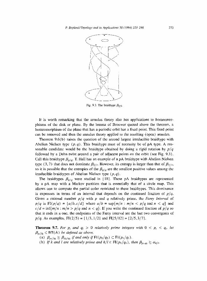
P Boyland/Topology and its Applications 58 (1994) 223-298 213
Fig. 9.3. The braidtype &5.
It is worth remarking that the annulus theory also has applications to homeomor-
phisms of the disk or plane. By the lemma of Brouwer quoted above the theorem, a
homeomorphism of the plane that has a periodic orbit has a fixed point. This fixed point
can be removed and then the annulus theory applied to the resulting (open) annulus.
Theorem 9.6(b) raises the question of the second largest irreducible braidtype with
Abelian Nielsen type (p, q). This braidtype must of necessity be of pA type. A rea-
sonable candidate would be the braidtype obtained by doing a rigid rotation by p/q
followed by a Dehn twist around a pair of adjacent points on the orbit (see Fig. 9.3).
Call this braidtype /S,)j4. T. Hall has an example of a pA braidtype with Abelian Nielsen
type (3,7) that does not dominate p3/7. However, its entropy is larger than that of p3/7,
so it is possible that the entropies of the &is are the smallest positive values among the
irreducible braidtypes of Abelian Nielsen type (p, q).
The braidtypes flPi4 were studied in [ 181. These pA braidtypes are represented
by a pA map with a Markov partition that is essentially that of a circle map. This
allows one to compute the partial order restricted to these braidtypes. This dominance
is expresses in terms of an interval that depends on the continued fraction of p/q.
Given a rational number p/q with p and q relatively prime, the Furey Interval of
p/q is FI(p/q) = [a/b,c/d] where a/b = sup{m/n : m/n < p/q and n < q} and
c/d = inf{m/n : m/n > p/q and n < q}. If you write the continued fraction of p/q so
that it ends in a one, the endpoints of the Farey interval are the last two convergents of
p/q. As examples, FI(2/5) = [l/3,1/2] and FI[5/12] = [2/5,3/7].
Theorem 9.7. For pi and qi > 0 relatively prime integers with 0 < pi < qi, let
pPilq, E BT(A) be defined as above.
(a) PP,/4, ?I PP2~y2 ifand only ifWp2/q2) c Wpl/ql). (b) If k and 1 are relatively prime and k/l E FI(pi/qi), then &,,y, t ffkJ[.

274 l? Boyland/Topology and ifs Applicafions 58 (1994) 223-298
If fl(p/q) = [a/b, c/d], one can also compute that the entropy of p,)lq is the log of
the largest root of (xb - 2) (xd - 2) = 3.
9.5. Examples
The attracting period 5 orbit of the map HB from Section 1.9 has Abelian Nielsen
type (2,5) and so by Theorem 9.6, the map has a periodic orbit with braidtype 1~215. We
can get much more information about its dynamics by noticing that after an appropriate
choice of conjugation we see that the braidtype of the attracting periodic orbit is actually
,l32/5. Theorem 9.7(b) then shows that He also has periodic orbit with braidtypes (YkJl
for all k/Z E [l/3,1/2] = FI[2/5]. Since, for example, FI[5/12] c FI[2/5], we have
also that Hg has a periodic orbit with braidtype &J,T.
Recall from Section 2.5 that the 3 fixed points of the map Hf, as illustrated in Fig. 2.2
are in different Nielsen classes. If we isotope the map to eliminate all fixed points on
the outer boundary, then each fixed point is alone in its Nielsen class. Since the fixed
points each have non-zero index, they are isotopy stable. Now the attracting period-3
orbit of Hp is obtained by blowing down the permuted boundary components. If we call
this orbit O( b, HP), it follows that any homeomorphism that has a periodic orbit with
the same braidtype as a(b, HP) also has these three fixed points, and further, the fixed
points must have the same linking number with the orbit as those shown in Fig. 2.2.
This illustrates the information we have eliminated in passing to braidtypes. All that is
encoded in the partial order on braidtypes is that there is a fixed point. It ignores the
additional information that there are always three fixed points with a specific linking
configuration (cf. [ 121) .
10. The train track algorithm of Bestvina and Handel, by T.D. Hall
The results of the previous sections (e.g. Theorems 7.7 and 9.2) clearly indicate
the importance of understanding the structure and dynamics of the Thurston-Nielsen
representative in an isotopy class. There is an algorithm due to Bestvina and Handel
[ 91 (see also [ 81) which allows one to compute this information given a specification
of the class in terms of, say, its action on ~1. The algorithm determines whether the
class is of reducible, pseudoAnosov, or finite order type; and in the pseudoAnosov case,
it finds a Markov partition for the pseudoAnosov representative of the class. Similar
algorithms for the restricted case of homeomorphisms of a punctured disc are given by
Franks and Misiurewicz [ 471, and by Los [ 941.
This section is an introduction to the paper of Bestvina and Handel. Instead of giving
a formal description of the algorithm, we shall simply present three examples of its
application in the restricted context of homeomorphisms of the disc punctured by a
periodic orbit: these examples illustrate the basic moves involved in the algorithm. Even
in this restricted setting, there are subtleties of the algorithm which we shall not touch
upon: the careful reader should turn to [9] for full details.

I? Boyland/Topology and ifs Applications 58 (1994) 223-298 275
Let f : D* + D2 be an orientation preserving homeomorphism, which has an interior
period n orbit A. Suppose (without loss of generality) that the points of A lie on the
horizontal diameter of the disc, labeled al,. . . , a, from left to right, so that the isotopy
class of f in S = D2 \ A can be represented by a braid /3 E B, as in Section 1.7. Let Pi
be a small circle centered on ai for each i, and write P for the union of the (disjoint)
circles Pj. Let G C S be a graph containing P which has a single vertex Ui on P, for each i, such
that the inclusion G + S is a homotopy equivalence (see Fig. 10.2, top). Given the
isotopy class of f, one can pick an induced graph map g : G + G which sends vertices
to vertices, and edges to edge-paths without backtracking, permuting the components
of P cyclically. This map defines a transition matrix M(G, g), whose ij entry is the
number of times that the g-image of the jth edge of G crosses the ith edge in either
direction: the topological entropy h(g) of g is the logarithm of the spectral radius of
M( G, g) : this is an upper bound for the minimal entropy in the isotopy class of f. The graph map g : G + G is said to be ejficient if for each edge E of G and each
integer k > 1, the edge path gk (E) does not backtrack. The idea of the algorithm is as
follows: if g : G + G is not efficient, then either there is a g-invariant proper subgraph
of G which strictly contains P and is not homotopy equivalent to P (in which case a
corresponding reduction of the isotopy class can be found), or it is possible to replace
G with a (topologically distinct) graph G’ such that the induced map g’ : G’ + G’ has
strictly smaller entropy than g. In making such changes, the following conditions are
preserved:
(1) G has no vertices of valence 1 or 2, and
(2) g(P) = P, and each Pi is a connected component of Pm = Up0 gvk( P) for
each i.
Condition ( 1) means that there is a bound (depending on n) on the size of the transition
matrix M(G,g), and hence that the set of possible entropies h(g) is locally finite in
[0, co). Thus there is a number N, depending on n and the entropy of the initial graph
map, such that either a reduction or an efficient map g : G + G must be found after
at most N steps. If an efficient map is found, it is straightforward to determine the
Thurston type of the isotopy class of f; and in the pseudoAnosov case, the action of g
on the edges of G \ P corresponds to the action of a pseudoAnosov representative on a
Markov partition.
We shall begin with a very simple example of a reducible isotopy class: this introduces
the most important move of the algorithm, namely folding. The second example is
pseudoAnosov: we shall explain how the dynamical structure of the pseudoAnosov
representative can be deduced from the efficient graph map. Finally, we shall give an
example of the finite order case.
The initial choice of graph G is arbitrary. In all of our examples, we shall follow
a convention which has the advantage that the action of the initial graph map g is
relatively easy to determine, and satisfies the technical condition (2) above. We shall
always place the vertex ~1 on the right of the circle PI, and the vertex un on the left of
the circle P,,; the other vertices ui are placed either on the top or on the bottom of the

216 P BoylandlTopology and its Applications 58 (1994) 223-298
corresponding circle Pi, in such a way that when we complete the graph by putting in
a straight edge from ui to ui+t for i = 1,. . . , n - 1, condition (2) is satisfied.
Before embarking on the examples, we give a list of the various moves used in the
algorithm, and indicate the first point in the examples where they appear. The moves
are described in terms of the map g : G + G, but the important point to note is that
they all preserve the isotopy class of the underlying map f : S + S.
1. Folding: Example 1 Step 1.
2. Subdividing: Example 2 Step 1.
3. Valence 1 isotopy: Example 2 Step 3.
4. Valence 2 isotopy: Example 2 Step 4.
5. Collapsing an invariant forest: Example 2 Step 5.
Example 10.1 (The reducible case). Consider the period 6 orbit corresponding to the
braid /3 = (~3~~201(+5(+3@4~3~2~1. The action of the isotopy class on the horizontal arcs
joining the punctures is depicted in Fig. 10.1.
,:;:::::c:, ___* e Fig. 10.1.
Choose the initial graph G in the way described earlier: to do this, begin with the
points of A which are preimages of “folds” in the above diagram, namely ~2, ~24, and
us. Pick the corresponding vertices ~2, ~4, and us to be on the top, bottom, and top of
their circles respectively, in order to satisfy condition (2). Then consider the preimage
~23 of ~4, and choose us on the top of P3 to satisfy condition (2). The graph G thus
constructed, and its image under the isotopy class of f, are shown in Fig. 10.2.
a b e
1 2 3
!
4 5 6
e
a
Fig. 10.2.
The circles Pi are oriented in the positive sense and labeled with the numbers 1 to 6;
the other edges are oriented from left to right, and labeled with the letters a to e. Given
any oriented edge E, denote by z the same edge oriented in the opposite direction. With

l? Boyland/Topology and its Applicafions 58 (1994) 223-298 277
this convention, the action of g : G + G can be described by a -+ cd, b ---f d, c + i&‘, --
d + bcTde, e + ed4cba (the action on the circles Pi is omitted in this description,
since they are permuted by g).
Let us now introduce some formalism which will enable us to determine whether or
not g is efficient. Let C denote the set of oriented edges {a,. . . , e,Zi, . . . ,Z}, and define
a map Dg : L + C which sends an edge E to the first edge traversed by g(E). Thus
the action of Dg can be represented by the diagram in Fig. 10.3.
b-d a e
i I I a- c-c- b-d ---;
Fig. 10.3.
Now the only way that there can be backtracking in gk(E) is for the edge path
gk-’ (E) to contain a word El E2, where Dg( El) = Dg( Ez). This arises when there
are two edges El and E2 which are identified by some power of Dg, and one of the
edge paths g(E) contains the juxtaposition FEZ. However the pairs of edges which are
identified by a power of Dg can be read off the above diagram: they are {d, e}, {b, a},
{Z,d} (all these are identified by Dg), and {c,b} (which are identified by Dg2). It
follows that there is backtracking in g*(a) (since g(a) contains the word cd), in g3 (c) ,
in g*(d) and g3(d), and in g2(e) and g3(e>.
The fundamental move of the algorithm is folding, which eliminates backtracking.
Step 1: Fold d and e. Concentrate on the backtracking which arises from the identi-
fication of Dg2(b) and Dg2(c). We have g(e) = g(z)Z Thus e is replaced by a new
edge e’ with e = de’. This gives rise to the graph G’ depicted in Fig. 10.4.
Fig. 10.4.
The new graph map g’ : G’ + G’ and the corresponding map Dg’ are given by
a + cd, b + d, c ---f cb, d + bczde = bcqe’, e’ + g(d)g( e) = Z (see Fig. 10.5).
We drop the primes on g, G, and e (this will be done automatically after each step
from now on). The cancellation in g(d) has eliminated the corresponding backtracking,
and has reduced the entropy of g. (This folding implicitly involves the step called pulling
tight in [ 91.)
There are still backtrackings arising from the identification of Dg( 5) and Dg( c) , and
from that of Dg( d) and Dg( C) . We fold again to eliminate the latter of these:
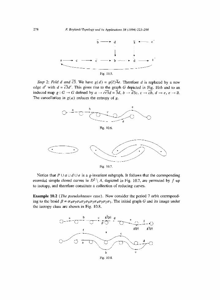
278 P. Boyland/Topology and its Applications 58 (1994) 223-298
b-d a e e’
i I a’“_“_;’
Fig. 10.5.
Step 2: Fold d and 3. We have g(d) = g(@e. Therefore d is replaced by a new edge d’ with d = zd’. This gives rise to the graph G depicted in Fig. 10.6 and to an induced map g : G --+ G defined by a 4 csd = ?5d, b 4 d3c, c --+ cb, d ---f e, e +Zi. The cancellation in g(u) reduces the entropy of g.
b e
a
Fig. 10.6.
- ‘-: Fig. 10.7.
Notice that P U a U d U e is a g-invariant subgraph. It follows that the corresponding
essential simple closed curves in D* \ A, depicted in Fig. 10.7, are permuted by f up
to isotopy, and therefore constitute a collection of reducing curves.
Example 10.2 (The pseudoAnosov case). Now consider the period 7 orbit correspond-
ing to the braid j? = ~4~5~4~3~6ff5~4U3~2U~. The initial graph G and its image under
the isotopy class are shown in Fig. 10.8.
b
Fig. 10.8.
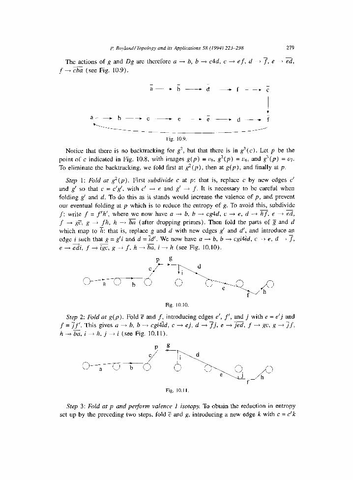
P. Boyland/Topology and its Applications 58 (1994) 223-298 279
The actions of g and Dg are therefore a + b, b + c4d, c 4 e f, d + 7, e + ed,
f + cba (see Fig. 10.9).
_ _ a- b-d-f- c
Fig. 10.9.
Notice that there is no backtracking for g2, but that there is in g3(c). Let p be the
point of c indicated in Fig. 10.8, with images g(p) = ug, g2(p) = ~4, and g3(p) = ~7.
To eliminate the backtracking, we fold first at g’(p), then at g(p), and finally at p.
Step 1: Fold at g2 (p). First subdivide c at p: that is, replace c by new edges c’
and g’ so that c = c’g’, with c’ + e and g’ + f. It is necessary to be careful when
folding g’ and d. To do this as it stands would increase the valence of p, and prevent
our eventual folding at p which is to reduce the entropy of g. To avoid this, subdivide - f: write f = f’h’, where we now have a + b, b ---f cg4d, c -+ e, d -+ h f, e -+ ed,
f - gC, g ---) fh, h + ba (after dropping primes). Then fold the parts of S and d
which map to h: that is, replace g and d with new edges g’ and d’, and introduce an
edge i such that g = g’i and d = id’. We now have a + b, b A cgi4?d, c -+ e, d + 7, - e + edi, f + igc, g 4 f, h + ba, i + h (see Fig. 10.10).
a 0 b
Fig. 10.10.
Step 2: Fold at g(p). Fold 2 and f, introducing edges e’, f’, and j with e = e’j and
f = Jf’. This gives a 7-
+ b, b --f cgi4d, c + ej, d -+ Tj, e 4 Jed, f --f si;, g + yf,
h -+ &, i + h, j + i (see Fig. 10.11).
a 0 b 0
h f
Fig. 10.11.
Step 3: Fold at p and perform valence 1 isotopy. To obtain the reduction in entropy
set up by the preceding two steps, fold C and g, introducing a new edge k with c = c’k

280 P BoylandlTopology and its Applications 58 (1994) 223-298
and g = kg’. However one end-point of k is a valence 1 vertex, and a valence I isotopy
can therefore be performed which pushes the edge k back into p. Therefore the only
effect of this step is that instead of c + ej and g ----f Jf, we now have c 4 e and
g + f. This operation has reduced the entropy.
Step 4: Perform Valence 2 isotopies. Finish off the procedure of steps 1 to 3 by
performing valence 2 isotopies to eliminate the two valence 2 vertices in G. Replace c
and g by a single edge c’ with c’ -+ e f; and postcompose by an isotopy which squeezes
the edge f down to the valence 3 vertex at its initial point, relabeling the edge h as f’.
We now have the graph shown in Fig. 10.12.
Fig. 10.12.
The actions of g and Dg are therefore a + b, b -+ ci4?d, c ---f e, d --f j, e + jed, - f -+ cba, i --+ f, j + i (see Fig. 10.13).
t a-b-c-e 7 -T-,- f
Fig. 10.13.
Step 5: Fold e and 2, and collapse invariant tree. There is now backtracking in g2 (e)
arising from the identification of e and d by Dg. Therefore e is replaced by a new
edge e’ with e = de’. Having done this, we have e’ --f 7: the edge e’ is therefore an
invariant tree, and it can be collapsed to a point by an isotopy. This yields the situation
of Fig. 10.14.
The actions of g and Dg are therefore a -+ b, b -+ ci4id, c ---f d, d --) j, f --f cba,
i 4 f, j --f i (see Fig. 10.15).
Step 6: Fold b and c, then 2i and b. Replace b with an edge b’ satisfying b = b’c,
and then fold again, replacing a and b’ with edges a’, b”, and e satisfying a = a? and
b’ = eb”. This gives Fig. 10.16.

Ff Boyland/Topology and its Applications 58 (1994) 223-298 281
f
Fig. 10.14.
Fig. 10.15.
f
Fig. 10.16.
The actions of g and Dg are therefore a -+ eb, b -+ i4E, c + 2, d + j, e -_) c,
f -+ ba, i + f, j + i (see Fig. 10.17).
c j-d-c-e--
-i-b
Fig. 10.17.
Step 7: Fold to eliminate backtracking in $(a). Notice that Dg4(Z> = Dg4( b). TO
eliminate the corresponding backtracking in $(a), perform the following sequence of
folds: (1) b = b’6j, (2) f = dsf’, (3) i = zi’, and (4) b = xb’.
These yield a + ?b67, b ---f i, c + 2, d -+ j, e -+ c, f ---f &2eZ, i + f, j -+ ai (see Fig. 10.18).
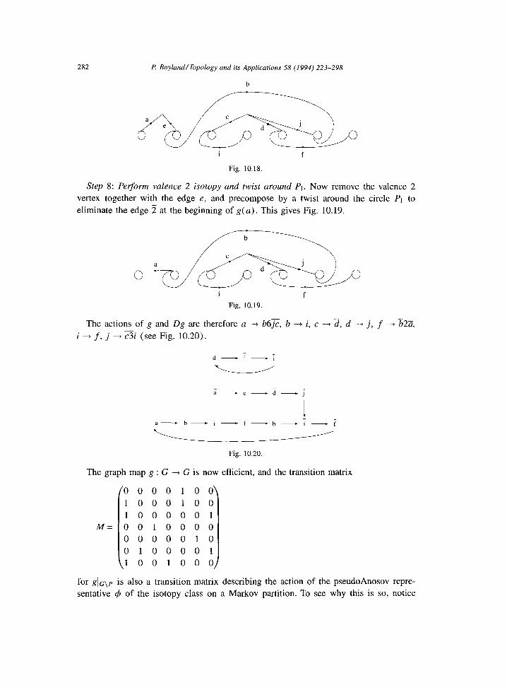
282 I? Boyland/Topology and its Applications 58 (1994) 223-298
b
i f
Fig. 10.18
Step 8: Peeorm valence 2 isotopy and twist around PI. Now remove the valence 2
vertex together with the edge e, and precompose by a twist around the circle P1 to
eliminate the edge 2 at the beginning of g(u). This gives Fig. 10.19.
i f
Fig. 10.19.
The actions of g and Dg are therefore a -+ b6jc, b -+ i, c -+ d, d --+ j, f -+ %!a,
i + f, j 4 zi (see Fig. 10.20).
i-c-d-j
Fig. 10.20.
The graph map g : G -+ G is now efficient, and the transition matrix
M=
lo 0 0 0 1 0 0
1000100
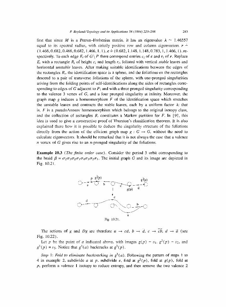
P: Boyland/Topology and ifs Applications 5R (1994) 223-298 283
first that since M is a Perron-Frobenius matrix, it has an eigenvalue A rv 1.46557
equal to its spectral radius, with strictly positive row and column eigenvectors r 4
(1.466,0.682,0.466,0.682, 1.466, 1, l), c A (0.682, 1.148, 1.148,0.783,1, 1.466, l),re-
spectively. To each edge E; of G\ P there correspond entries ci of c and rl of r. Replace
Ei with a rectangle Ri of height c, and length r-i, foliated with vertical stable leaves and
horizontal unstable leaves. After making suitable identifications between the edges of
the rectangles Ri, the identification space is a sphere, and the foliations on the rectangles
descend to a pair of transverse foliations of the sphere, with one-pronged singularities
arising from the folding points of self-identifications along the sides of rectangles corre-
sponding to edges of G adjacent to P; and with a three pronged singularity corresponding
to the valence 3 vertex of G, and a four pronged singularity at infinity. Moreover, the
graph map g induces a homeomorphism F of the identification space which stretches
the unstable leaves and contracts the stable leaves, each by a uniform factor A: that
is, F is a pseudoAnosov homeomorphism which belongs to the original isotopy class,
and the collection of rectangles R, constitutes a Markov partition for F. In [9], this
idea is used to give a constructive proof of Thurston’s classification theorem. It is also
explained there how it is possible to deduce the singularity structure of the foliations
directly from the action of the efficient graph map g : G + G, without the need to
calculate eigenvectors. It should be remarked that it is not always the case that a valence
n vertex of G gives rise to an n-pronged singularity of the foliations.
Example 10.3 (The jinite order case). Consider the period 5 orbit corresponding to
the braid p = V2~3(~2uiff4(~3(~2(T1. The initial graph G and its image are depicted in
Fig. 10.21.
p STP) 93(P)
0
c d
0
a
Fig. 10.21.
The actions of g and Dg are therefore a -+ cd, b + d, c ---) cb, d -t Zi (see
Fig. 10.22).
Let p be the point of a indicated above, with images g(p) = ~4, g2(p) = ~2, and
g3 (p) = vg. Notice that g3( a) backtracks at g3 (p).
Step 1: Fold to eliminate backtracking in g3( a). Following the pattern of steps 1 to
4 in example 2, subdivide a at p, subdivide e, fold at g2(p), fold at g(p), fold at
p, perform a valence 1 isotopy to reduce entropy, and then remove the two valence 2
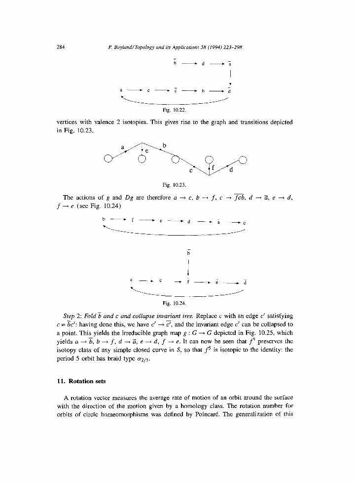
284 P Boyland/Topology and its Applications 58 (1994) 223-298
a+6 Fig. 10.22.
vertices with valence 2 isotopies. This gives rise to the graph and transitions depicted
in Fig. 10.23.
Fig. 10.23.
- The actions of g and Dg are therefore a -+ c, b --f f, c -+ fcb, d -+ a, e t d,
f -+ e (see Fig. 10.24)
aii Fig. 10.24.
Step 2: Fold b and c and collapse invariant tree. Replace c with an edge c’ satisfying
c = k’: having done this, we have c’ + c’, and the invariant edge c’ can be collapsed to
a point. This yields the irreducible graph map g : G --f G depicted in Fig. 10.25, which
yields a + b, b -+ f, d -+ 3, e --f d, f -+ e. It can now be seen that f5 preserves the
isotopy class of any simple closed curve in S, so that f is isotopic to the identity: the
period 5 orbit has braid type 1x215.
11. Rotation sets
A rotation vector measures the average rate of motion of an orbit around the surface
with the direction of the motion given by a homology class. The rotation number for
orbits of circle homeomorphisms was defined by Poincare. The generalization of this
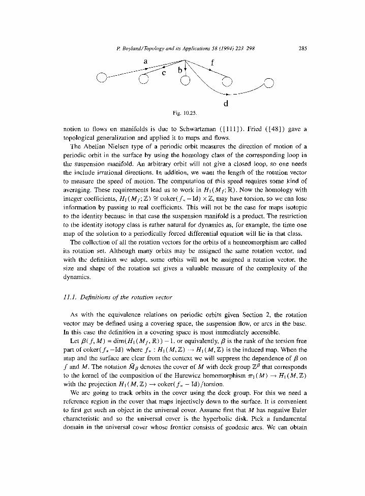
E Boyland/Topology and its Applications 58 (1994) 223-298 285
d Fig. 10.25
notion to flows on manifolds is due to Schwartzman ( [ 1111). Fried ( [48] ) gave a
topological generalization and applied it to maps and flows.
The Abelian Nielsen type of a periodic orbit measures the direction of motion of a
periodic orbit in the surface by using the homology class of the corresponding loop in
the suspension manifold. An arbitrary orbit will not give a closed loop, so one needs
the include irrational directions. In addition, we want the length of the rotation vector
to measure the speed of motion. The computation of this speed requires some kind of
averaging. These requirements lead us to work in Ht (Mf; R). Now the homology with
integer coefficients, Hi (Mf; Z) 2 coker( f* -Id) x Z, may have torsion, so we can lose
information by passing to real coefficients. This will not be the case for maps isotopic
to the identity because in that case the suspension manifold is a product. The restriction
to the identity isotopy class is rather natural for dynamics as, for example, the time one
map of the solution to a periodically forced differential equation will lie in that class.
The collection of all the rotation vectors for the orbits of a homeomorphism are called
its rotation set. Although many orbits may be assigned the same rotation vector, and
with the definition we adopt, some orbits will not be assigned a rotation vector, the
size and shape of the rotation set gives a valuable measure of the complexity of the
dynamics.
11.1. Definitions of the rotation vector
As with the equivalence relations on periodic orbits given Section 2, the rotation
vector may be defined using a covering space, the suspension flow, or arcs in the base.
In this case the definition in a covering space is most immediately accessible.
Let /3( f, M) = dim( Hi (Mf, IR) ) - 1, or equivalently, p is the rank of the torsion free
part of coker( f* -Id) where f* : HI (M, Z) -+ HI (M, Z) is the induced map. When the
map and the surface are clear from the context we will suppress the dependence of p on
f and M. The notation a, denotes the cover of A4 with deck group Zfl that corresponds
to the kernel of the composition of the Hurewicz homomorphism ~1 (M) + HI (M, Z)
with the projection HI (M, Z) + coker( f* - Id) /torsion.
We are going to track orbits in the cover using the deck group. For this we need a
reference region in the cover that maps injectively down to the surface. It is convenient
to first get such an object in the universal cover. Assume first that M has negative Euler
characteristic and so the universal cover is the hyperbolic disk. Pick a fundamental
domain in the universal cover whose frontier consists of geodesic arcs. We can obtain

286 P. BoylandlTopology and its Applications 58 (1994) 223-298
M by pairwise identifying edges of this fundamental domain. Now let ij be obtained
from this fundamental domain by removing one of each of the identified edges and
replacing or removing corners when necessary so that D projects injectively down into
the surface. If M is the torus or the annulus, the construction is similar.
Now let D be the projection of d to fip. Note that D has compact closure and if
r : fip + M is the projection, rr restricted to D is injective. Thus tip = Ua( D), where the disjoint union is over all CT E Zk. Define a (discontinuous) map r : I$?, ---f izp
via r( 2) = CT if R E (T(D). Now fix a lift _? : &lp + h?lp and a lift Z of n E M, and
define the rotation vector of x as
p(x, f) = lim r(f”‘(_f>) - r(R)
i-boo i
if the limit exists. Since r commutes with all deck transformations, the rotation vector
does not depend on the choice of lift of the point x. However, it does depend on choice
of J, and so it is only defined up to translation by an element from Zp. The rotation
set of f is p(f) = {p(x, f) : x E M}.
If we let A : M + Zp be the projection to M of the equivariant map r ( f( 2) ) - r (2) :
b?p --+ Zp, then A gives the approximate displacement of any lift of the point X. Given
a f-invariant probability measure ,LL, we can define its rotation vector as p( ,u) = J A dp.
This rotation vector measures the average displacement of points with respect to the
measure ,u. By the Birkhoff ergodic theorem (see Section 1.2), if ,u is ergodic, then for
p-almost every point x, p(x, f) = p(p).
The definition of the rotation vector using arcs is somewhat unnatural in the general
situation, so it will be deferred until we restrict to the identity isotopy class. The
definition using the suspension flow uses a family of arcs to non-dynamically close
orbits so they can be treated as homology classes. The specifics of the family of arcs
are eliminated by passing to a limit. This definition is essentially that of the homology
direction of an orbit given in [48].
In the “half-open” fundamental domain b in the universal cover pick a base point .Q
and for each I E D, an arc CX c l? with gX(0) =X0 and (?lx( 1) = R. The arc (Y, is the
projection of CX to M.
Recall from Section 2.1 that the suspension flow was denoted $t and that MO c Mf
is MO = p( M x (0)) where p : M x R + Mf is the projection. We may identify MO
with M and think of the arcs (Y, as subsets of MO. For each x E MO and n E Pi let
Thus y( x, n) is the loop constructed by starting at the basepoint x0, going to x via
the closing loop (Y, and then flowing forward by the suspension flow for n units of
time. This puts us at the point fn(x) in MO, and we go back to the basepoint xo via
the inverse of the closing loop ‘YF~(,). Recall that Ht (Mf; R) S E-Xp x JR. For a class
b E HI (Mf; IR), let pt (b) be the projection of b on the first factor and then
P. Boyland/Topology and ifs Applicarions 58 (I 994) 223-298 28-l
p(x, f) = ,,im PI ( [74x, 4 I) 1-03 i
when the limit exists, where [ y(x, i)] is the homology class representing the closed
loop y(x, i) in HI (Mf, R). Now there is ambiguity since we have chosen generators
for Hl(Mf,lFC).
If 0(x, f) is a periodic orbit recall that its Abelian Nielsen type is the element
in HI (Mf, Z) g coker(f, - Id) x Z that is represented by its orbit in the suspen-
sion. If (v, n) is the image of ant(x, f) under the projection coker(f, - Id) x Z ---f
coker( f* - Id) /torsion x Z = Zp x Z, then p( x, f) will be the vector v/n E lRfl.
11.2. Rotation sets of pA maps
It should be clear by now that pA maps have complicated dynamics. The next theorem
gives another expression of this fact using rotation sets. The rotation set of a pA map is
always convex and top-dimewional. This implies, among other things, that their periodic
orbits span homology in the suspension.
Let C$ be a pA map. In [ 481 and [ 491, Fried showed that the closure of the collection
of rotation vectors of periodic orbits of 4 is a P-dimensional convex set. In addition,
this convex set is the convex hull of the rotation vectors of periodic orbits that come
from minimal loops (see Section 1.3) in the Markov model for c,z~. The question of
whether every vector in this convex set comes from some orbit was answered in the
case of pA maps rel finite sets on the torus in [ 1031 (see Theorem 11.8). The proof
the author knows of the general result below is due to Kwapisz.
Theorem 11.1. If q5 : M ---f M is a pA map and p = /3( f, M), then p(4) c Iwp is a
closed, @dimensional set that is the convex hull of the rotation vectors of the periodic
orbit coming from minimal loops in the Markov model of 4. Furthel; if u E Int(p(Q)),
then there is a compact, &invariant set X,, with p( x, @) = u for all x t X,. Thus there
is an ergodic, invariant probability measure ,uu,, with p(p(.) = u. If u E Qp nInt(p(+)),
then we can choose X,, to be a periodic orbit.
The basic idea of the proof is illustrated by the examples in Sections 1.3 and 11.7. The
existence of the ergodic invariant measure supported in X,. follows from the standard
fact that any compact invariant set contains the support of an ergodic measure. Note
that the last sentence of the theorem says nothing about the period of the periodic orbit
that has a given rotation vector. In particular, it may not have an uncollapsible Abelian
Nielsen type.
The next result follows from Theorem 7.4(b) and the previous theorem. The main
observation needed is that orbits that globally shadow will have the same rotation vectors.
Corollary 11.2. If q!~ is a pA homeomorphism and g Y 4, then p( 4) c p(g) and so,
in particulal; p(g) has interior.
288 I? BoylandITopology and its Applications 58 (1994) 223-298
Theorem 7.4(b) also implies that any u E p( q5) n p(g) will be represented by some
g-invariant set Y,. This set will be the preimage of the &invariant set X, under the
semi-conjugacy.
11.3. Homeomorphisms isotopic to the identity
Now we restrict attention to just those f that are isotopic to the identity. In this
case 16’j~ is the universal abelian cover of M, i.e. it has deck group isomorphic to
HI (M, Z) = Zp where p, the first Betti number, is twice the genus if M is closed, and
2g + (b - 1) when there is boundary. The suspension manifold is a product M x S’ and
H1(Mf,Z) = H,(M,Z) x Z.
The definition of the rotation vector using arcs appears in [43] and [44]. Let fi :
id N f be an isotopy to f from the identity, and let ux be the trace of the isotopy that
connects x and f(x), i.e. gx( t) = f,(x). Now given x and II E N, let w(x, n) be the
class represented by a, . cx gfcx) . . . . . CT~-I(~) . (CUE)-’ where the (Y’S are the
closing arcs used in the definition with the suspension flow. One can check that
p(x, f) = &z 4x, Q/i
when the limit exists.
The information given in Theorem 11.1 is only valid for pA maps. For general maps
isotopic to the identity we study the rotation set using a now familiar strategy; find
finite invariant sets A so that the map is hidden pA rel A, and then use isotopy stability
results to apply Theorem 11.1 to these maps.
The next result is the analog of Theorem 11.1 for relative pA maps $. Note that we
are just measuring the rotation set of 4 in the ambient manifold, not in the manifold
punctured by the finite invariant set.
Theorem 11.3. If c$ : M + M is isotopic to the identity and there is ajnite $-invariant
set A so that q!~ is pA rel A, then ~(4) c Iwo is a closed, P-dimensional convex set
where p is the first Betti-number of M. Further; if u E Int(p(+)), then there is a
compact, &invariant set X, with p(x, 4) = u or all x E X,,. Thus there is an ergodic, f invariant probability measure ,q, with p(,~~,) = v. If u E QP n Int(p( 4)), then we can
choose XL, to be a periodic orbit.
We will formulate the analog of Corollary 11.2 in terms of strong Nielsen types. As
with the rotation number and entropy, we can also associate a rotation set to a strong
Nielsen type. If p E SNT( M, id), let pset(/3) = p(@p), where @p is a TN-condensed
map that represents 0. In this case we do not assume that @p is pA, so we need to use
Theorem 7.7.
Corollary 11.4. If f is isotopic to the identity and p E snt( f), then p,,t(p) C ,o( f). In particulal; if p is of pA type, then p(f) has interior.
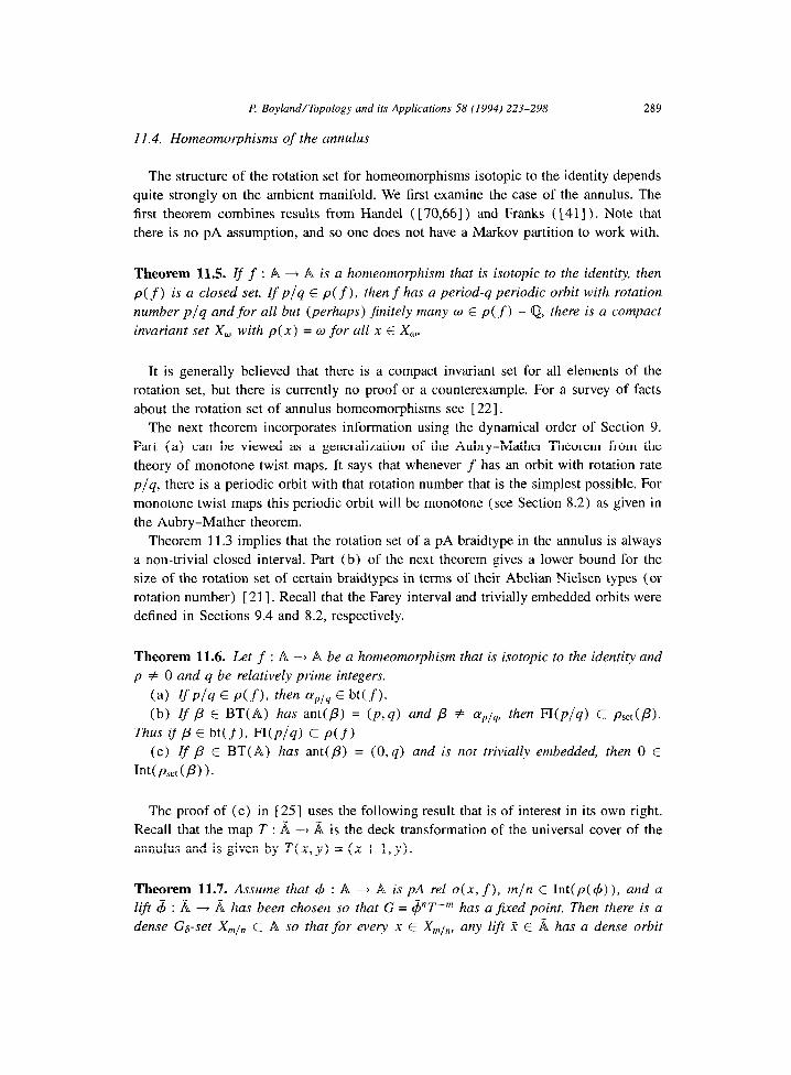
F? Boyland/Topology and its Applications 58 (1994) 223-298 289
11.4. Homeomorphisms of the annulus
The structure of the rotation set for homeomorphisms isotopic to the identity depends
quite strongly on the ambient manifold. We first examine the case of the annulus. The
first theorem combines results from Handel ( [ 70,661) and Franks ( [41] ). Note that
there is no pA assumption, and so one does not have a Markov partition to work with.
Theorem 11.5. Zf f : A + A is a homeomorphism that is isotopic to the identity, then
p(f) is a closed set. If p/q E p( f ), then f has a period-q periodic orbit with rotation
number p/q and for all but (perhaps) finitely many w E p(f) - Q, there is a compact
invariant set X, with p(x) = o for all x E X,.
It is generally believed that there is a compact invariant set for all elements of the
rotation set, but there is currently no proof or a counterexample. For a survey of facts
about the rotation set of annulus homeomorphisms see [22].
The next theorem incorporates information using the dynamical order of Section 9.
Part (a) can be viewed as a generalization of the Aubry-Mather Theorem from the
theory of monotone twist maps. It says that whenever f has an orbit with rotation rate
p/q, there is a periodic orbit with that rotation number that is the simplest possible. For
monotone twist maps this periodic orbit will be monotone (see Section 8.2) as given in
the Aubry-Mather theorem.
Theorem 11.3 implies that the rotation set of a pA braidtype in the annulus is always
a non-trivial closed interval. Part (b) of the next theorem gives a lower bound for the
size of the rotation set of certain braidtypes in terms of their Abelian Nielsen types (or
rotation number) [ 211. Recall that the Farey interval and trivially embedded orbits were
defined in Sections 9.4 and 8.2, respectively.
Theorem 11.6. Let f : A -+ A be a homeomorphism that is isotopic to the identity and
p # 0 and q be relatively prime integers.
(a) VP/q E p(f), then aplq E Wf). (b) IfP E BT(A) has ant(P) = (p,q) and P + ap/q, then n(p/q) c pSet(P).
Thus ifP~ bt(f)> Wplq) c p(f) (c) Zf p E BT(A) has ant(p) = (0, q) and is not trivially embedded, then 0 E
WpS&P) ).
The proof of (c) in [25] uses the following result that is of interest in its own right.
Recall that the map T : & + I% is the deck transformation of the universal cover of the
annulus and is given by T(x,y) = (x + 1,~).
Theorem 11.7. Assume that C$ : A + A is pA rel 0(x, f), m/n E Int(p(ti)), and a
lift 4 : I% + I% has been chosen so that G = $“T-“’ has a jixed point. Then there is a
dense Ga-set X,1,, c A so that for every x E X,,,,,, any lift i E d has a dense orbit
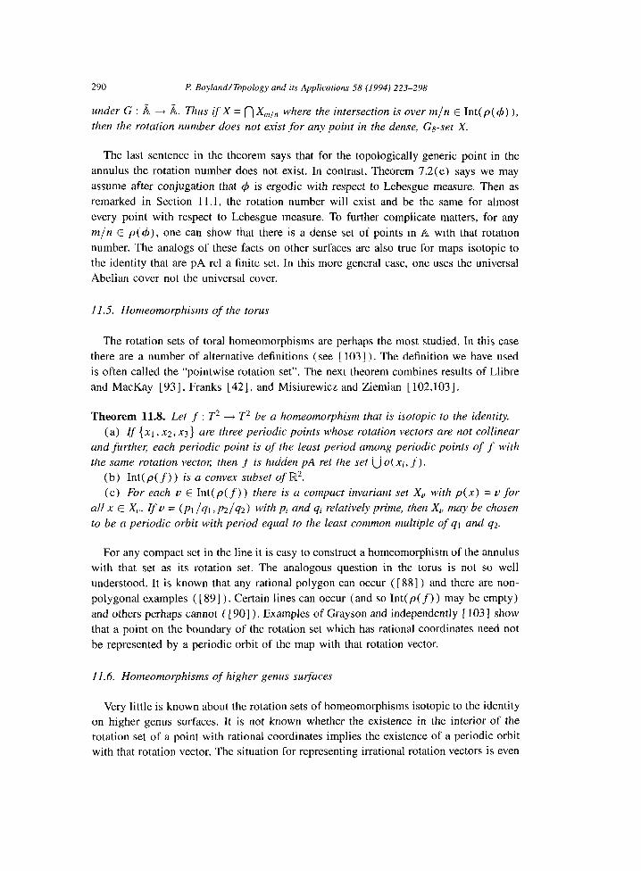
290 P Boyland/Topology and its Applications 58 (1994) 223-298
under G : B + A. Thus if X = n X,,,,, where the intersection is over m/n E Int( p( 4) ),
then the rotation number does not exist for any point in the dense, Gs-set X.
The last sentence in the theorem says that for the topologically generic point in the
annulus the rotation number does not exist. In contrast, Theorem 7.2(e) says we may
assume after conjugation that 4 is ergodic with respect to Lebesgue measure. Then as
remarked in Section 11.1, the rotation number will exist and be the same for almost
every point with respect to Lebesgue measure. To further complicate matters, for any
m/n E p( 4)) one can show that there is a dense set of points in A with that rotation
number. The analogs of these facts on other surfaces are also true for maps isotopic to
the identity that are pA rel a finite set. In this more general case, one uses the universal
Abelian cover not the universal cover.
11.5. Homeomorphisms of the torus
The rotation sets of toral homeomorphisms are perhaps the most studied. In this case
there are a number of alternative definitions (see [ 1031). The definition we have used
is often called the “pointwise rotation set”. The next theorem combines results of Llibre
and MacKay [93], Franks [42], and Misiurewicz and Ziemian [ 102,103].
Theorem 11.8. Let f : T2 + T2 be a homeomorphism that is isotopic to the identity.
(a) If {xl, x2, x3) are three periodic points whose rotation vectors are not collinear
and furthen each periodic point is of the least period among periodic points of f with
the same rotation vector; then f is hidden pA rel the set U o(xi, f).
(b) Int( p( f) ) is a convex subset of IR2.
(c) For each u E Int( p( f)) there is a compact invariant set X, with p(x) = o for
~11 x E X,,. If u = (~1 /ql , p2/q2) with pi and qi relatively prime, then X, may be chosen
to be a periodic orbit with period equal to the least common multiple of q1 and q2.
For any compact set in the line it is easy to construct a homeomorphism of the annulus
with that set as its rotation set. The analogous question in the torus is not so well
understood. It is known that any rational polygon can occur ([ 881) and there are non-
polygonal examples ( [ 891) . Certain lines can occur (and so Int( p( f) ) may be empty)
and others perhaps cannot ( [ 901). Examples of Grayson and independently [ 1031 show
that a point on the boundary of the rotation set which has rational coordinates need not
be represented by a periodic orbit of the map with that rotation vector.
11.6. Homeomorphisms of higher genus surfaces
Very little is known about the rotation sets of homeomorphisms isotopic to the identity
on higher genus surfaces. It is not known whether the existence in the interior of the
rotation set of a point with rational coordinates implies the existence of a periodic orbit
with that rotation vector. The situation for representing irrational rotation vectors is even

I? Boyland/Topology and its Applications 58 (1994) 223-298 291
less clear. The main difficulty in higher genus is that the rotation set is defined using
the universal Abelian cover which is now no longer the plane. In particular, Brouwer’s
Lemma (see Section 9.4) and its extensions (e.g. [ 41,421) no longer hold. The universal
cover is the plane, but the deck group there is non-Abelian, and it is not clear how to
translate the homology information of rotation vectors into homotopy information for
use in the universal cover. Franks ( [ 43,441) and Handel (personal communication)
have made some progress with “homotopy” rotation vectors. For the case of flows on
surfaces see [ 1181 and [2].
There is an analog of Theorem 11.8(a) that works on higher genus surfaces. On the
torus, Theorem 11.8(a) can be used to get the invariant sets representing non-rational
rotation vectors because given three non-collinear points with rational coordinates in the
interior of the rotation set, Theorem 11.8(c) allows one to represent these points with
periodic orbits. One then uses Theorem 11.8(a) to get a hidden pA rel these orbits, and
then Theorem 11.3 and isotopy stability to get invariant sets for other points inside the
triangle spanned by the points. This strategy does not work in higher genus because of
the remarks of the previous paragraph.
We restrict now to the case of closed surfaces. For cq , (~2 E HI (M; Z) , let I (q , ~2)
be their algebraic intersection number. Since we are assuming that f P id, Ht (Mf; Z) =
Ht (M; Z) x Z. The Abelian Nielsen type of an orbit can thus be written as ant( x, f) =
(p(x), n) where p(x) is a homology class in M and n is the period of the orbit. This
means that p(x) just keeps track of the direction of the orbit in M and neglects the
speed, so it is called the homology direction of the orbit (this is a slightly different
use of this term from Fried [49] ). The following theorem arose in a conversation with
J. Franks.
Theorem 11.9. If M is a closed sueace of genus g > 1 and f : M ---f M is a
homeomorphism isotopic to the identity that has a collection of periodic orbits X =
(x1 3 x2,. . .1 xk} with k > 1 whose homology directions are linearly independent in E%‘g
and further satisfy I (p( xi), p( xi+, ) ) + 0 for i = 1,. . . , k - 1, then f has a hidden pA
component rel X and convexhull((0) U {p(xl), . . . ,p(xk))} c p(f).
The proof is fairly standard. One examines the various possibilities for reducing
curves of the isotopy class rel X and then sees what the Thurston-Nielsen types of the
components can be. It turns out that there must be a pA component that contains all of
X and then one uses Theorem 11.3. The presence of the zero in the convex hull comes
from the fact that any homeomorphism of a surface with negative Euler characteristic
has a fixed point.
11.7. Examples
We continue the analysis of the homeomorphism Hk of Section 1.9. This homeo-
morphism is defined on the annulus minus five open disks: let us call this space As.
Now HI (AS; Z) g IT?, and we can identify the generators geometrically as one of the

292 I? Boyland/Topology and its Applications 58 (1994) 223-298
Fig. 11.1. The covering space fip for the map Ha
boundary components of the annulus and the boundaries of the 5 removed disks. Now
HL induces a cyclic permutation of these last 5 generators and is the identity on the
first. Thus coker( (HL), - Id) = Z2, and so the integer homology of the suspension
manifold is Z3. Each of the three components has a geometric interpretation. The first
keeps track of how many times around the annulus a loop goes. The second coordinate
measures the linking number of a loop with the suspension of the permuted boundary
components, and the third is the period. The rotation set of Hk will then be a subset of
R*, and we can interpret the first component of a rotation vector as the usual rotation
number in the annulus and the second as a “linking rate” about the permuted boundary
components. The 2’ cover that detects these motions is shown in Fig. 11.1.
To compute the rotation set we examine the motion of the Markov partition in the
Z2 cover in a manner similar to the one used in examples in Sections 1.3 and 3.4. First
choose a lift of HL that fixes the back edge of the cover and call this lift Z?. Next pick
a fundamental domain in the cover and lift the Markov partition in the base to five
rectangles in the fundamental domain denoted Ri. We keep track of the motion of a
rectangle in the cover by using the symbols r and e in the transition matrix. The symbol Y
represents the horizontal deck transformation as in Fig. 11.1. It records motions around
the annulus. The symbol ! represents the vertical deck transformation and it records
linking information. In the augmented transition matrix we write PP’ in the (i, j) th
place if 8( I?i) n fi( r’V’( l?j) # 8, and 0 otherwise. It is fairly straightforward to
compute that
0 0 c e2 0 00100
B"= 0 0 0 1 1 .
i 1
roe 00
0 r r! i-e2 0
In Section 1.3 we computed the minimal loops of this process and as in that section
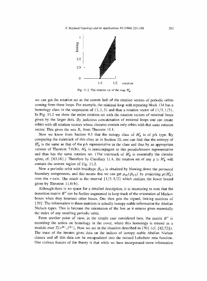
l? Boyland/Topology and its Applications 58 (1994) 223-298 293
113 112 rotation
Fig. 11.2. The rotation set of the map Hk
we can get the rotation set as the convex hull of the rotation vectors of periodic orbits
coming from these loops. For example, the minimal loop with repeating block 134 has a
homology class in the suspension of ( 1 , 1,3) and thus a rotation vector of ( l/3, l/3).
In Fig. 11.2 we show the entire rotation set with the rotation vectors of minimal loops
given by the larger dots. By judicious concatenation of minimal loops one can create
orbits with all rotation vectors whose closures contain only orbits with that same rotation
vector. This gives the sets X,, from Theorem 11.1.
Now we know from Section 9.5 that the isotopy class of Hh is of pA type. By
computing the traintrack of this class as in Section 10, one can find that the entropy of
Hk is the same as that of the pA representative in the class and thus by an appropriate
version of Theorem 7.6(b), Hk is semiconjugate to this pseudoAnosov representative
and thus has the same rotation set. (The traintrack of Hk is essentially the circular
spine, cf. [63,18].) Therefore by Corollary 11.4, the rotation set of any g pv H(B will
contain the convex region of Fig. 11.2.
Now a periodic orbit with braidtype &S is obtained by blowing down the permuted
boundary components, and this means that we can get p,,,( &s) by projecting p( HL) onto the r-axis. The result is the interval [l/3,1/2] which realizes the lower bound
given by Theorem 11.6(b)
Although there is no space for a detailed description, it is interesting to note that the
transition matrix B” can be further augmented to keep track of the orientation of Markov
boxes when they intersect other boxes. One then gets the signed, linking matrices of
[ 391. The information in these matrices is actually isotopy stable information for Abelian
Nielsen types. This is because the orientation of the box as it returns gives essentially
the index of any resulting periodic orbit.
From another point of view, in the simple case considered here, the matrix B” is
recording the action on homology in the cover, where this homology is treated as a
module over Z[ Y*‘, !*’ I. Now we are in the situation described in [ 501 (cf. [ 82,721).
The trace of the iterates gives data on the indices of isotopy stable Abelian Nielsen
classes and all this data can be encapsulated into the twisted Lefschetz zeta function.
One curious feature of the theory is that while we have incorporated more information
294 P. Boylrnd/Topology and ifs Applications 58 (1994) 223-298
in the matrix by including the signs, now there can be cancellation upon iteration, so
we can lose information. At first this seems counterintuitive, but on second thought it
is seen as a consequence of the fact that the signed matrix records isotopy stable data,
so cancellation must be allowed as the index of various classes must add and perhaps
cancel. The inclusion of signs in the transition matrix also allows it to be used for
entropy estimates ( [ 53,521)
We leave it to the reader to use the computations of Section 3.4 to compute that
rotation set of Hk is [ -1, 11. This rotation set could perhaps be called the “linking
interval”.
Notes and acknowledgments
In writing a survey article the author must decide what to cover, how to cover it, and
how to reference it. Even in the area of topological methods in surface dynamics I have
been unable to discuss all the interesting work. I have focused on what could be called
the methods of low-dimensional topology and have neglected some very important work
using continuum theory, inverse limits and prime ends. Connections to knot theory have
been neglected as well as work on area-preserving maps. In many cases the references
will provide just a starting point to the literature. I have not tried for an exhaustive
bibliography or history.
I have chosen to focus on theorems and examples. The reader is referred to the
literature for the proofs. There is a certain amount of material that is new, or else
folklore, in which case proofs do not exist in the literature. The proofs of most this type
of material will appear in [ 241.
The first iterate of this paper was the lecture notes [20]. I would like to thank R.
MacKay for organizing those lectures and C. Carroll. J. Guaschi, and T. Hall for taking
and preparing the notes. This paper was prepared to accompany a mini-course at the
Summer Conference on General Topology and Applications, Amsterdam, August, 1994.
I would like to thank the organizers for this opportunity and especially J. van Mill and
J.M. Aarts for their help with the manuscript.
Thanks to T. Hall, S. van Strien and J. Kwapisz for useful comments on the
manuscript, and special thanks to T. Hall for allowing me to use Section 10, a sec-
tion from our forthcoming book. This paper has benefited greatly from conversations
with and the work of J. Franks, D. Fried, M. Handel and B. Jiang. A good way to
pursue the topics in this paper is to read their papers.
A special acknowledgment is due to the work of Bob Williams which pioneered many
of the applications of low dimensional topology to dynamics that are used in this paper.
References
[I ] L. Alseda, J. Llibre and M. Misiurewicz, Combinatorial Dynamics and Entropy in Dimension One (World Scientific, Singapore, 1993).
P: Boyland/Topology and its Applicutions 58 (1994) 223-298 295
[2] S.Kh. Aranson and V.Z. Grimes, Topological classification of flows on closed two-dimensional
manifolds, Russ. Math. Surveys 41 ( 1986) 183-208. [ 31 V.I. Amol’d, Geometrical Methods in the Theory of Ordinary Differential Equations (Springer, Berlin,
2nd ed., 1988). [4] D. Asimov and J. Franks, Unremovable closed orbits, in: J. Palis, eds., Geometric Dynamics, Lecture
Notes in Math. 1007 (Springer, Berlin, 1983) 22-29 (revised version in preprint).
] 5 ] S. Batterson and J. Smillie, Filtrations and periodic data on surfaces, Amer. J. Math. 108 ( 1986)
193-234. [6] D. Benardete, M. Gutierrez and Z. Nitecki, Braids and the Thurston-Nielsen classification, preprint,
Tufts University, 199 1. [ 71 L. Bers, An extremal problem for quasiconformal mappings, Acta. Math. 141 ( 1978) 73-98.
[ 81 M. Bestvina and M. Handel, Train tracks and automorphisms of free groups, Ann. Math. 135 ( 1992)
I-51. [9] M. Bestvina and M. Handel, Train tracks for surface homeomorphisms, preprint, CUNY, 1992.
1 lo] .I. Birman, Braids, Links and Mapping Class Groups, Annals of Mathematics Studies (Princeton Univ.
Press, Princeton, NJ, 1975).
[ 111 J. Birman and M. Kidwell, Fixed points of psuedo-Anosov diffeomorphisms of surfaces, Adv. Math.
46 (1982) 73-98.
[ 121 I. Birman and R. Williams, Knotted periodic orbits in dynamical systems 11: knot holders for fibered
knots, Contemp. Math. 20 ( 1983) l-60. [ 131 P Blanchard and J. Franks, The dynamical complexity of orientation reversing homeomorphisms of
surfaces, Invent. Math. 62 ( 1980) 333-339. [ 141 L. Block and W. Coppel, Dynamics in one dimension, Lecture Notes in Math. 1513 (Springer, Berlin,
1992). [ 151 C. Bonatti, J.M. Gambaudo, J.L. Lion and C. Tresser, Wandering domains for infinitely renormalizable
diffeomorphisms of the disk, preprint, Universite de Nice Sophia-Antipolis, 1993.
1161 R. Bowen, Entropy and the fundamental group, in : N. Markeley, J. Martin and W. Perrizon, eds.,
The structure of Attrators in Dynamical Systems, Lecture Notes in Math. 668 (Springer, Berlin, 1978)
21-30. [ 171 P Boyland, Braidtypes and a topological method of proving positive entropy, preprint, Boston
University, 1984. [ 18 ] P. Boyland, An analog of Sharkovski’s theorem for twist maps, Contemp. Math. 81 (1988) 119-133.
[ 19 1 P. Boyland, Rotation sets and Morse decompositions for twist maps, Ergod. Theor. Dynam. Sys. 8’
(1988) 33-61.
[ 201 P Boyland, Notes on dynamics of surface homeomorphisms: lectures by P. Boyland and J. Franks,
notes by C. Carroll, J. Guaschi and T. Hall, August 1989, Warwick, pp. l-48.
1211 F! Boyland, Rotation sets and monotone orbits for annulus homeomorphisms, Comm. Math. Helv. 67 (1992) 203-213.
1221 P. Boyland, The rotation set as a dynamical invariant, in: Proceedings of the IMA Workshop on Twist Maps, IMA Volumes in Math. Appl. 44 (Springer, Berlin, 1992).
[23] I? Boyland, Isotopy stability for dynamics on surfaces, IMS preprint 93/10, SUNY at Stony Brook, NY, 1993.
[ 241 P. Boyland and T. Hall, Dynamics of surface homeomorphisms (World Scientific, Singapore, to appear),
[25] P Boyland, T. Hall and J. Guaschi, L’ensemble de rotation des homeomorphismes pseudo-Anosov, C.
R. Acad. Sci. Paris. SCr I Math. 316 (1993) 1077-1080.
1261 L. Brouwer, Uber die periodischen transformationen der Kugel, Math. Ann. 80 ( 1919) 39-41, 1271 R.F. Brown, The Lefschetz Fixed Point Theorem (Scott, Foresman & Co., Glenview, IL, 1971).
[28 1 P Brunovsky, On one parameter families of diffeomorphisms 1 and 11, Comment. Math. Univ. Carolin.
11 ( 1970) 559-582 and 12 ( 1970) 765-784.
1291 A. Casson and S. Bleiler, Automorphisms of Surfaces after Nielsen and Thurston, London Math. Sot.
Stud. Texts 9 (Cambridge Univ. Press, Cambridge, 1988).
[ 301 IF! Cornfield, S.V. Fomin and Ya.G. Sinai, Ergodic Theory (Springer, Berlin, 1982). [31] W. de Melo and J. van Strien, One-Dimensional Dynamics (Springer, Berlin, 1993).
1321 R. Devaney, An Introduction to Chaotic Dynamical Systems (Addison-Wesley, Reading, MA, 1989). [33] S. Eilenberg, Sur les transformations periodiques de la surface de sphere, Fund. Math. 22 (1934)
228-244.

296 R Boyland/Topology and its Applications 58 (1994) 223-298
1341 E. Fade11 and S. Husseini, Fixed point theory for non-simply connected manifolds, Topology 20 ( 198 1) 53-92.
[35] E. Fade11 and S. Husseini, The Nielsen number on surfaces, Contemp. Math. 21 (1983) 59-98.
[36] A. Fathi, Homotopy stability of pseudo-Anosov diffeomorphisms, Ergod. Theor. Dynam. Sys. 10 ( 1989) 287-294.
[ 371 A. Fathi, E Lauderbach and V. Poenaru, Travaux de Thurston sur les surfaces, Asterique 66-67 ( 1979).
[38] J. Franks, Anosov diffeomorphisms, in: AMS Proceedings of Symposia in Pure Mathematics XIV (AMS, Providence, RI, 1979) 61-93.
[39] J. Franks, Knots, links and symbolic dynamics, Ann. Math. 113 (1981) 529-552.
(401 J. Franks, Homology and Dynamical Systems, CBMS 49 (AMS, Providence, RI, 1982).
[41] J. Franks, Recurrence and fixed points of surface homeomorphisms, Ergod. Theor. Dynam. Sys. 8*
(1988) 99-107.
[ 421 J. Franks, Realizing rotation vectors for torus homeomorphism, Trans. AMS 311 (1989) 107-I 15.
1431 J. Franks, Geodesics on S2 and periodic points of annulus diffeomorphisms, preprint, Northwestern
University, 1993.
[44] J. Franks, Rotation vectors and fixed points of area preserving surface diffeomorphisms, preprint, Northwestern University, 1994.
[45] J. Franks, and M. Handel, Entropy and exponential growth of rrt in dimension two, Proc. AMS, 102 (1988) 753-760.
[46] J. Franks and M. Misiurewicz, Rotation sets of toral flows, Proc. Amer. Math. Sot. 109 (1990)
243-249.
[ 471 J. Franks and M. Misiurewicz, Cycles for disk homeomorphisms and thick trees, in: [ 991, 69-l 39.
[48] D. Fried, Flow equivalence, hyperbolic systems and a new zeta function for flows, Comm. Math. Helv.
57 (1982) 237-259.
1491 D. Fried, The geometry of cross sections to flows, Topology 24 (1983) 353-371.
[SO] D. Fried, Periodic orbits and twisted coefficients, in: J. Palis, eds., Geometric Dynamics, Lecture Notes
in Math. 1007 (Springer, Berlin, 1983) 261-293.
[51] D. Fried Homological identities for closed orbits, Invent, Math. 71 (1983) 419-442.
[52] D. Fried, Growth rate of surface homeomorphisms and Row equivalence, Ergod. Theor. Dynam. Sys. 5
(1985) 539-563.
[53] D. Fried, Entropy and twisted cohomology, Topology 25 (1986) 455-470.
[54] D. Fried, Lefschetz formulas for flows, Contemp. Math. 58 (1987) 19-69.
[ 551 EB. Fuller, The treatment of periodic orbits by methods of fixed point theory, Bull. AMS 72 ( 1966) 838-840.
[ 561 J.M. Gambaudo, D. Sullivan and C. Tresser, Infinite cascades of braids and smooth dynamical systems,
Topology 33 (1994) 85-94.
[57] J.M. Gambaudo, S. van Strien and C. Tresser, The periodic orbit structure of of orientation preserving
diffeomorphisms of D* with topological entropy zero, Ann. Inst. H. Poincare 49 (1989) 335-356.
[58] M. Gerber and A. Katok, Smooth models of Thurston’s pseudo-Anosov maps, Ann. Sci. I& Norm.
Sup. 15 (1982) 173-204.
[ 591 J. Guckenheimer and P. Holmes, Nonlinear Oscillations, Dynamical Systems, and Bifurcations of Vector
Fields (Springer, Berlin, 1983).
[60] G.R. Hall, A topological theorem of a theorem of Mather’s on twist maps, Ergod. Theor. Dynam. Sys.
4 (1984) 585-603.
[61] T. Hall, Unremovable periodic orbits of homeomorphisms, Math. Proc. Camb. Phil. Sot. 110 ( 1991)
523-531.
[62] T. Hall, Weak universality in two-dimensional transitions to chaos, Phys. Rev. Len. 71 (1993) 58-61.
1631 T. Hall, Fat one-dimensional representatives of pseudo-Anosov isotopy classes with minimal periodic
orbit structure, Nonlinearity 7 (1994) 367-384. 1641 T. Hall, The creation of horseshoes, Nonlinearity 7 (1994) 861-924.
[ 651 M. Handel, The entropy of orientation reversing homeomorphisms of surfaces, Topology 21 (1982) 291-296.
1661 M. Handel, Zero entropy surface homeomorphisms, preprint, C.U.N.Y., 1988.
[67] M. Handel, Global shadowing of pseudo-Anosov homeomorphisms, Ergod. Theor. Dynam. Sys. 5 (1985) 373-377.
P Boyland/Topology and ifs Applicafions 58 (1994) 223-298 297
1681 M. Handel, Entropy and semi-conjugacy in dimension two, Etgod. Theor. Dynam. Sys. 9 (1989)
585-596.
[69] M. Handel, Approximating entropy by exponential growth of ~1 in dimension two, preprint, C.U.N.Y.,
1989.
[70] M. Handel, The rotation set of a homeomorphism of the annulus is closed, Comm. Math. Phys. 127
( 1990) 339-349.
[71] K. Hiraide, Expansive homeomorphisms of compact surfaces are pseudo-Anosov, Osaka J. Math. 27
(1990) 117-162.
172) H.-H. Huang and B. Jiang, Braids and periodic solutions, in: B. Jiang, ed., Topolgical Fixed Point
Theory and Applications, Lecture Notes in Math. 1411 (Springer, Berlin, 1989) 107-123.
[73] N.V. lvanov, Entropy and Nielsen numbers, Soviet Math. Dokl. 26 (1982) 63-66.
[74] N.V. lvanov, Nielsen numbers of self-maps of surfaces, J. Soviet Math. 26 (1984) 1636-1641.
[75] N.V. Ivanov, Subgroups of Teichmuller modular groups, Translations of Mathematical Monographs,
Vol. 115 (AMS, Providence, RI, 1992).
[ 761 B. Jiang, Fixed point classes from a differentiable viewpoint, in: E. Faddel and G. Foumier, eds., Fixed
Point Theory, Lecture Notes in Math. 886 (Springer, Berlin, 1981) 163-170.
[77] B. Jiang, Fixed points of surface homeomotphisms, Bull. AMS 5 (1981) 176-178.
1781 B. Jiang, Lectures on Nielsen Fixed Point Theory, Contemp. Math. 14 (AMS, Providence, RI, 1983).
1791 B. Jiang, Fixed points and braids I, Invent. Math. 75 (1984) 69-74.
[ 801 B. Jiang, Fixed points and braids II, Math. Ann. 272 (1985) 249-256.
[ 811 B. Jiang, A characterization of fixed point classes, Contemp. Math. 72 (1988) 157-160.
[ 821 B. Jiang, Estimation of the number of periodic orbits, preprint, Peking University, 1994.
[83] B. Jiang and J. Guo, Fixed points of surface diffeomorphisms, Pacific J. Math. 160 ( 1993) 67-89.
[ 841 A. Katok, Bernoulli diffeomorphisms on surfaces, Ann. Math. 110 ( 1979) 529-547.
[ 851 A. Katok, Lyapunov exponents, entropy and periodic orbits for diffeomorphisms, Publ. Math. IHES 51
(1980) 137-173.
[ 861 A. Katok, Nonuniform hyperbolicity and the structure of smooth dynamical systems, in: Proc. Intemat.
Congress of Math. Warsaw (1983) 1245-1253.
[ 871 B. Kerekjarto, Sur la structure des transformations topologiques des surfaces en elles-memes, Enseign.
Math. 35 (1936) 297-316.
[ 881 J. Kwapisz, Every convex polygon with rational vertices is a rotation set, Ergod. Theor. Dynam. Sys.
12 (1992) 333-339.
[89] J. Kwapisz, A nonpolygonal rotation set, SUNY at Stony Brook, 1994.
[90] P. Le Calvez, Proprietes dynamiques des diffeomorphismes de l’anneau et du tore, Asterisque 204
(1991).
[911 J. Lewowicz, Expansive homeomorphisms of surfaces, Bol. Sot. Bras. Mat. 20 ( 1989) 113-133.
1921 J. Lewowicz and L. de SB, Analytic models of pseudo-Anosov maps, Ergod. Theor. Dynam. Sys. 6
(1986) 385-392.
1931 J. Llibre and R.S. MacKay, Rotation vectors and entropy for homeomorphisms of the torus isotopic to the identity, Ergod. Theor. Dynam. Sys. 11 (1991) 115-128.
[94] J. Los, Pseudo-Anosov maps and invariant train tracks in the disc: a finite algorithm, Proc. London Math. Sot. 66 (1993) 400-430.
]95] J. Los, On the forcing relation for surface homeomotphisms, preprint, Universite de Nice Sophia- Antipolis, 1994.
[ 961 R. Mane, Ergodic Theory and Differentiable Dynamics (Springer, Berlin, 1987).
1971 T. Matsuoka, Braids of periodic points and a 2-dimensional analogue of Sharkovskii’s ordering, in: G.
lkegami, ed., Dynamical systems and nonlinear oscillations, (World Scientific Press, 1986) 58-72.
[98] T. Matsuoka, The Burau representation of the braid group and the Nielsen-Thurston classification, in: [99], 21-41.
1991 C.K. McCord, ed., Nielsen Theory and Dynamical Systems, Contemp. Math. 152 (AMS, Providence,
RI, 1993).
[ 1OOJ K.R. Meyer and G.R. Hall, Introduction to Hamiltonian Dynamical Systems and the N-Body Problem, Applied Mathematical Sciences 90 (Springer, Berlin, 1992)
[ 101 J M. Misiurewicz, Formalism for studying periodic orbits of one-dimensional maps, in: S. Alsina, ed., European Conference on Iteration Theory (World Scientific, Singapore, 1989) l-7.

298 P Boyland/Topology and its Applications 58 (1994) 223-298
[ 1021 M. Misiurewicz and K. Ziemian, Rotation sets for maps of tori, J. London Math. Sot. 40 ( 1989) 490-506.
[ 1031 M. Misiurewicz and K. Ziemian, Rotation sets and ergodic measures for torus homeomorphisms, Fund. Math. 137 (1991) 45-52.
[104] S. Newhouse, Lectures on dynamical systems, in: J. Moser, J. Guckenheimer and S Newhouse, Dynamical Systems: C.I.M.E. Lectures, Progress in Math. 8 (Birhluser, Basel, 1980) l-l 14.
[ 1051 R. Penner and J. Harer, Combinatorics of Train Tracks, Annals of Math. Studies 125 (Princeton Univ. Press, Princeton, NJ, 1992).
[ 1061 R. Plytkin, Sources and sinks for A-diffeomorphisms, USSR Math. Sb. 23 (1974) 233-253.
[ 1071 M. Pollicott, Lectures on Ergodic Theory and Pesin Theory on Compact Manifolds, London Math. Sot.
Lecture Note Series 180 (Cambridge Univ. Press, Cambridge, 1993). [ 1081 M. Rees, A minimal positive entropy homeomorphism of the two torus, J. London Math. Sot. 23
(1981) 537-550.
[ 1091 C. Robinson, Introduction to the Theory of Dynamical Systems (CRC Press, Boca Raton, FL, to
appear). [ 1 lo] D. Ruelle, Elements of Differentiable Dynamics and Bifurcation Theory, (Academic Press, New York,
1989).
[ 1111 S. Schwa&man, Asymptotic cycles, Ann. Math. 66 ( 1957) 270-284.
[ 1121 A. Sharkovski, Coexistence of cycles of a continuous map of a line into itself, Ukrain. Mat. Z. 16
(1964) 61-71.
[ 1131 M. Shub, Global stability of dynamical systems (Springer, Berlin, 1987).
[ 1141 J. Smillie, Periodic points of surface homeomorphisms with zero entropy, Ergod. Theor. Dynam. Sys.
3 (1983) 315-334. [ 1151 P. Stefan, A theorem of Sharkovski on the existence of periodic orbits of continuous endomorphisms
of the real line, Comm. Math. Phys. (1977) 237-248. [ 1161 W. Thurston, On the geometry and dynamics of diffeomorphisms of surfaces, Bull. AMS 19 (1988)
417-431. [ 1171 F. Vivaldi, Arithmetic theory of Anosov diffeomorphisms, Proc. Roy. Sot. London Ser. A 413 ( 1987)
97-107. [ 1181 J. Walsh, Directions for structurally stable flows via rotation vectors, preprint, Oberlin University, 1994.
[ 1191 P. Walters, An Introduction to Ergodic Theory, Graduate Texts in Math. 79 (Springer, Berlin, 1982).