Topological Inference for ModernData Analysis

An Introduction to Persistent Homology

Giancarlo Sanchez

A project presented for the degree of

Master’s of Science in Mathematics

Department of Mathematics and Statistics

Florida International University

Graduate Advisor: Dr. Miroslav Yotov

April 29, 2016

Abstract

Persistent homology has become the main tool in topological data analysis be-cause of it’s rich mathematical theory, ease of computation and the wealth of pos-sible applications. This paper surveys the reasoning for considering the use oftopology in the analysis of high dimensional data sets and lays out the mathemati-cal theory needed to do so. The fundamental results that make persistent homologya valid and useful tool for studying data are discussed and finally we compute ex-amples using the package TDA available in the CRAN library for the statisticalprogramming language R.

Data & Geometry

The modern data analyst’s biggest challenge is dealing with tremendous amounts ofcomplex data. Not only is it difficult to deal with the enormous amounts of observationsbeing stored, but also in the amount of attributes or features being measured in theprocess. Advances in computing power have made it easier to analyze high dimensionaldata and it has been proven very beneficial for companies and scientists alike to extractuseful information from these high dimensional data sets. Many companies even collectdata without knowing beforehand if the data will ever be analyzed, let alone how. Thishas pushed forward the rise of data science as an extremely interesting and necessaryfield of study as it stands at the intersection of modern mathematics, statistics, computerscience and an enormous amount of applications.

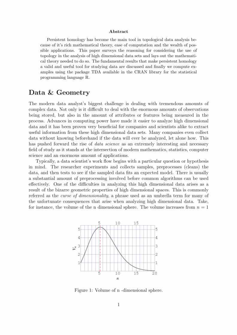
Typically, a data scientist’s work flow begins with a particular question or hypothesisin mind. The researcher experiments and collects samples, preprocesses (cleans) thedata, and then tests to see if the sampled data fits an expected model. There is usuallya substantial amount of preprocessing involved before common algorithms can be usedeffectively. One of the difficulties in analyzing this high dimensional data arises as aresult of the bizarre geometric properties of high dimensional spaces. This is commonlyreferred as the curse of dimensionality, a phrase used as an umbrella term for many ofthe unfortunate consequences that arise when analyzing high dimensional data. Take,for instance, the volume of the n dimensional sphere. The volume increases from n = 1

Figure 1: Volume of n -dimensional sphere.

1

to n = 5 and then rapidly decreases to 0 from n = 20 and beyond. Consider also themultivariate standard Gaussian distribution scaled to have integral equal to 1. It is wellknow that 90% of the volume falls within a radius of 1.65 of the mean for the single variatecase. This percentage rapidly decreases to 0 as the dimension of the Gaussian functionincreases. This means that much of the data is found in the tails of the distribution,far, far away from center. More trouble arises when attempting to learn models in themachine learning sense.[1] Since the models used for learning are only valid in the range orvolume in which the data are available, as the dimensions increase we must collect moreand more data to fill up the space. For example, for a simple linear regression model withone explanatory variable, we might be satisfied with collecting 10 observations before wetry to learn the model. A linear regression model with 2 explanatory variables mustthen need 100 observations collected and 1000 for a 3-dimensional model and so on. Thenumber of samples needed grows exponentially as the dimension of the feature variablesincreases. Models and algorithms generally do not behave well when scaling these highdimensions. However, while these data sets do seem large at first glance, it is common tosee data sparsely floating around in these higher dimensions while actual artifacts tendto be living within a simpler, lower dimensional structure. Therefore, a big componentof the preprocessing phase is the time spent transforming data into a simpler space orselecting unimportant features to disregard in the analysis.

Geometric intuition has paved the way for various methods in data analysis whichaim at reducing this excess in dimensionality. Traditional tools like Principal ComponentAnalysis, while maintaining the largest variance among points, linearly projects pointsonto a lower dimensional subspace. While other linear techniques are useful, much modernresearch has been devoted to nonlinear dimensionality techniques (collectively known asmanifold learning) and follow similar geometric frameworks to data reduction. In it,we assume that the data were originally sampled from a sub-manifold that is of lowerdimension than the ambient space. We try to find a nonlinear space that describes thedata well and is in bijection with smaller sub-manifold. The problem of dealing withhigh dimensions typically gets worse with nonlinear methods since they involve muchmore parameters to be estimated.

Nevertheless, geometry has been very influential in the design of many data analysisalgorithms and techniques. Our intuition guides us well in 2 or 3 dimensions, yet thecounter-intuitive geometry of higher dimensions causes us to lack insight. To understandthe basic structure of the data, more qualitative information is needed. Geometry itselfis concerned with questions of size, shape, and relative positions of objects. For example,it provides the tools to be able to mathematically differentiate a circle from a square -which can be unnecessary in data analysis if all we needed to know was that there wasa hole in the middle of this data for some circle-like data set. Information about thetopology of the underlying space in which the data were sampled from provides us withqualitative information that is useful in this analysis

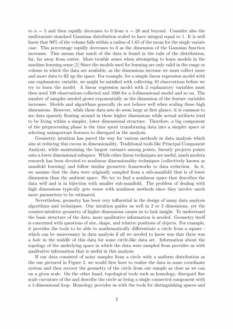
If our data consisted of noisy samples from a circle with a uniform distribution asthe one pictured in Figure 2, we would first have to realize the data in some coordinatesystem and then recover the geometry of the circle from our sample as close as we canon a given scale. On the other hand, topological tools such as homology, disregard finescale curvature of the and describe the circle as being a single connected component witha 1-dimensional loop. Homology provides us with the tools for distinguishing spaces and

2

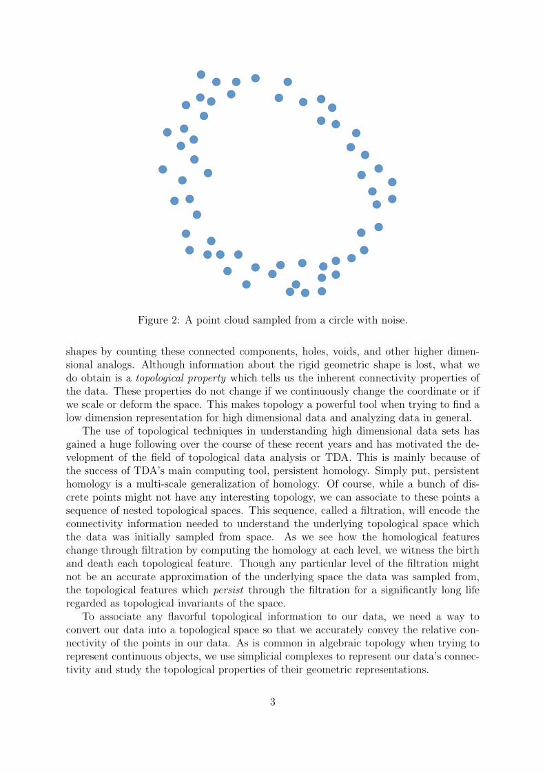
Figure 2: A point cloud sampled from a circle with noise.

shapes by counting these connected components, holes, voids, and other higher dimen-sional analogs. Although information about the rigid geometric shape is lost, what wedo obtain is a topological property which tells us the inherent connectivity properties ofthe data. These properties do not change if we continuously change the coordinate or ifwe scale or deform the space. This makes topology a powerful tool when trying to find alow dimension representation for high dimensional data and analyzing data in general.

The use of topological techniques in understanding high dimensional data sets hasgained a huge following over the course of these recent years and has motivated the de-velopment of the field of topological data analysis or TDA. This is mainly because ofthe success of TDA’s main computing tool, persistent homology. Simply put, persistenthomology is a multi-scale generalization of homology. Of course, while a bunch of dis-crete points might not have any interesting topology, we can associate to these points asequence of nested topological spaces. This sequence, called a filtration, will encode theconnectivity information needed to understand the underlying topological space whichthe data was initially sampled from space. As we see how the homological featureschange through filtration by computing the homology at each level, we witness the birthand death each topological feature. Though any particular level of the filtration mightnot be an accurate approximation of the underlying space the data was sampled from,the topological features which persist through the filtration for a significantly long liferegarded as topological invariants of the space.

To associate any flavorful topological information to our data, we need a way toconvert our data into a topological space so that we accurately convey the relative con-nectivity of the points in our data. As is common in algebraic topology when trying torepresent continuous objects, we use simplicial complexes to represent our data’s connec-tivity and study the topological properties of their geometric representations.

3

From Data to Simplcial Complexes

Characters and landscapes seen in video games are a great example of how simplicialcomplexes provide great approximations of continuous surfaces, as anyone who has everplayed a video game would attest. In TDA, we try to approximate two distinct points’similarity by using simplicial complexes. If points are similar, we keep them in the samecomplex, if they are different, we keep them as separate ones. Similarity can be defined byeuclidean distance though many other metrics are used. Typically, a similarity measureis chosen by a domain expert. The data set X, sometimes referred to as a point cloud,consists of samples from a space X ⊂ Rd. We try to infer the topological information ofX using only the sample points and their relative distances. To approximate X though,we first turn convert our data into a simplicial complex. This produces an easy to workwith topological object that contains needed connectivity information of X and if oursample is dense enough, provides a real good approximation of the topological invariantsof the original space X. There are many ways of constructing a simplicial complex from adiscrete point cloud. Each construction provides a similar approximation of the underly-ing structure of the data. They differ when it comes to the computational considerations.In this section we introduce simplical complexes and two fundamental constructions usedin persistent homology, the Cech complex and the Vietoris-Rips complex.

Simplicial Complexes & The Nerve

Figure 3: Geometric representation of low dimensional simplex.

Simplexes are the building blocks of simplicial complexes. A point is a 0-dimensionalsimplex, a line is a 1-dimensional simplex, and a solid triangle is a 2-dimensional simplex.A 3-dimensional simplex can be thought of as a tetrahedron but it’s difficult to imagineany higher dimensional n-simplex. Geometrically one can define simplicial complexesby gluing together simplicies along their faces in a nice way (in some ambient spaceRd). There is an equivalent combinatorial representation of any simplicial complex whichmakes discussing some of their properties much smoother.

Definition. Given a finite vertex set V = {1, ...n}, a simplicial complex Σ is acollection of subsets of V such that if σ ∈ Σ and σ′ ⊂ σ then σ′ ∈ Σ.

We’ll normally consider our point cloud as the finite vertex set V = X and try to findsimplicial complex with a topology which closely approximates the underlying space X.

4

We call an element σ ∈ Σ a simplex and the dimension of σ is one less than the cardinality,dim(σ) = |σ| − 1 . The dimension of the simplicial complex Σ is the highest dimensionamong all it’s simplex. A nonempty proper subset of a simplex γ ⊂ σ is called a face ofσ and by definition is also a simplex. A simplicial complex that is a subset of a simplicialcomplex Γ ⊂ Σ is called a simplicial subcomplex. There exists a function that sends eachsimplex in Γ to itself in Σ known as the inclusion map ι : Γ→ Σ. More generally, we candefine a function between any two arbitrary simplicial complexes so long the vertices ofeach n-dimensional simplex are mapped to the verticies of a target simplex. That is, ifΣ1 and Σ2 are 2 simplicial complexes, a function f from the vertex set of Σ1 to the vertexset of Σ2 is a simplical map if for all σ ∈ Σ1, we have that f(σ) ∈ Σ2. It is important tonote that any simplical map could only send n-simplicies to m-simplicies where m ≤ n.

We can construct a simplical complex for any collection of sets based on how the setsintersect. More specifically, for a given open cover U = {Uα}α∈A of a topological space X,the nerve of U denoted by N (U), is defined to be the simplicial complex with vertex setA and a k dimensional simplex σ = {α0, ...αk} ∈ N (U) if and only if Uα0 ∩ ...∩Uαk

6= ∅ .There is a condition that guarantees when the nerve of the cover will stay faithful to thetopology of the underlying space.

Nerve Lemma. Suppose that X and U are as above, and suppose that the covering isnumerable. Suppose further that for all ∅ 6= S ⊂ A, we have that

⋂s∈S US is either

contractible or empty. Then N (U) is homotopy equivalent to X.

The Nerve Lemma is a basic result which guarantees that N (U) is of the same homotopytype as the underlying space X.

Cech & Vietoris-Rips Complexes

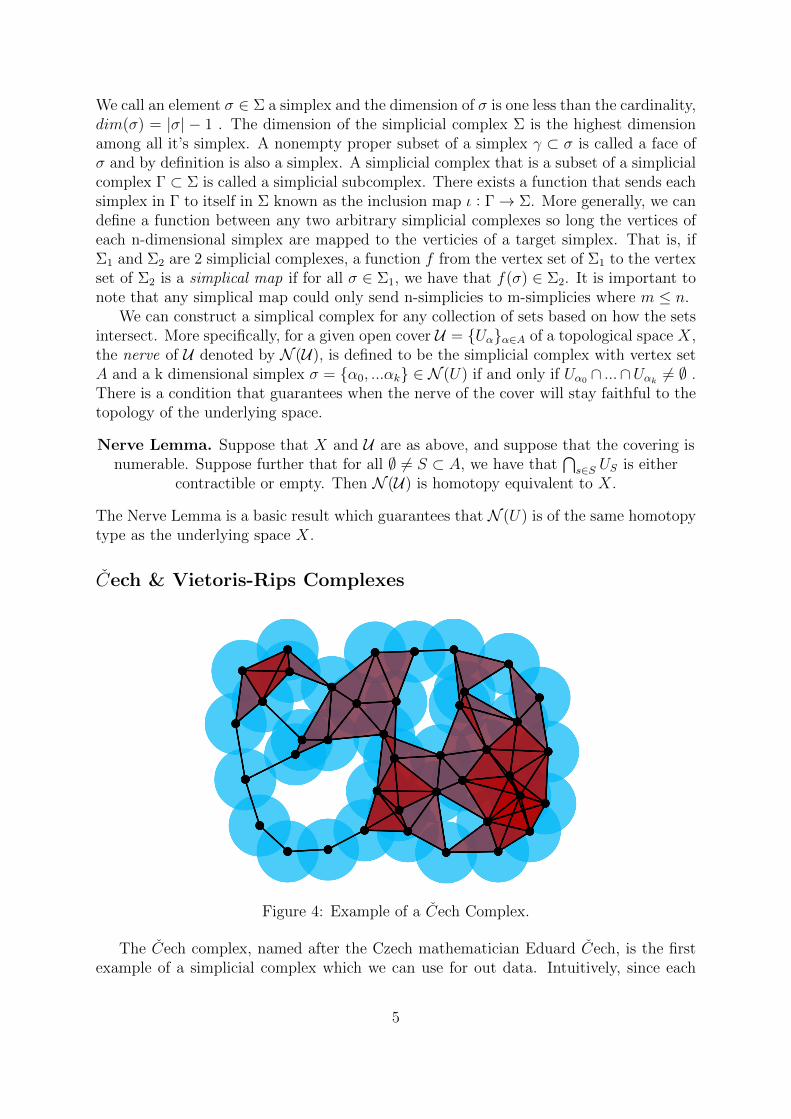
Figure 4: Example of a Cech Complex.

The Cech complex, named after the Czech mathematician Eduard Cech, is the firstexample of a simplicial complex which we can use for out data. Intuitively, since each

5

point should lie on or around the space X, if we make our points bigger and have enoughof them, we should be able to give a good approximation of X. Mathematically, we canconsider each point as the center of an open ball of fixed radius ε > 0 denoted byBε(x) :={y : d(x, y) < ε}. The collection of these ε balls makes a cover Bε = {Bε(x) : x ∈ X} ofour point cloud.

Definition. A Cech complex is the nerve of the covering of balls,Cε(X) := N (Bε) = {σ ⊂ X :

⋂x∈σ Bε(x) 6= ∅}.

That is, Cε(X) is the simplicial complex obtained by considering X as our vertex setand {x1, ..., xk+1} span a k-simplex if and only if

⋂k+1i=1 Bε(xi) 6= ∅. Since the ε-balls are

each convex, their intersection is convex (hence contractible) and thus the Nerve Lemmaapplies. Cech complex is homotopy equivalent to the union of balls, which should be arough estimation of our space. Therefore if we want to learn about our point cloud wecan pick an ε and study the topology of it’s corresponding Cech complex. Notice that fora smaller radius ε′ < ε, the smaller Cech Complex Cε′ is a subcomplex. In turn, we getan inclusion map ι : Cε′ → Cε of complexes. For a small enough value, we’ll have a Cechcomplex consisting of n 0-dimensional simplices. For a large enough value, we’ll havesingle (n-1)-dimensional simplex. As ε increases we will obtain a finite nested sequence ofCech complexes and inclusion maps. Each of these spaces approximates the underlyingspace at different scales. The problem comes when finding the right scale to consider outdata. The idea of persistent homology is to study all scales simultaneous and record howtopological features evolve as the scale changes. The Cech complex filtration is a goodway to imagine how evolution at different scales occurs and, moreover, why importanttopological features should persist.

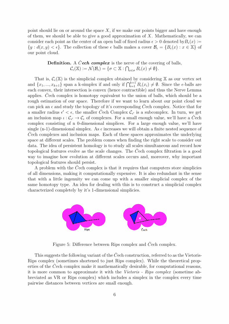
A problem with the Cech complex is that it requires that computers store simpliciesof all dimensions, making it computationally expensive. It is also redundant in the sensethat with a little ingenuity we can come up with a smaller simplicial complex of thesame homotopy type. An idea for dealing with this is to construct a simplicial complexcharacterized completely by it’s 1-dimensional simplicies.

Figure 5: Difference between Rips complex and Cech complex.

This suggests the following variant of the Cech construction, referred to as the Vietoris-Rips complex (sometimes shortened to just Rips complex). While the theoretical prop-erties of the Cech complex make it mathematically desirable, for computational reasons,it is more common to approximate it with the Vietoris - Rips complex (sometime ab-breviated as VR or Rips complex) which includes a simplex in the complex every timepairwise distances between vertices are small enough.

6

Definition. Given ε > 0, a Vietoris-Rips complex on X is the simplicial complexRε(X) := {σ ⊂ X : ∀x, y ∈ σ,Bε(x) ∩Bε(y) 6= ∅}

That is, we include a k-simplex if for points {x1, ..., xk+1}, the distance between any twopoints is d(xi, xj) < 2ε for all 1 ≤ i, j,≤ k. Notice that we also get an inclusion Rε′ ⊂ Rε

for ε′ ≤ ε. The VR complex is easier to compute since only pairwise distances need to becalculated in order to obtain our simplicial complex. Moreover, it’s easily seen that wehave the inclusion Cε(X) ⊂ Rε(X). In fact, the collection of 1-simplicies is equal for bothcomplexes so the VR complex is the largest complex that can made given the collectionof 1 simplicies from a Cech complex. Even though the VR complex will be generallylarger than the Cech complex, they satisfy the sandwich relation,

Cε(X) ⊂ Rε(X) ⊂ C2ε(X).

This means that if the Cech complex is a good approximation of X, then so will the VRcomplex - even though we don’t have a guarantee that the VR complex is of the samehomotopy type of any particular space.

Other Complexes

The Cech and VR complexes are generally very large simplicial complexes and there aremany ways that we can reduce some of the redundancy of information. Much researchin topological data analysis is directed towards finding efficient simplicial complexes torepresent to the data. The following are some alternatives usually considered.

Delaunay Complex

For each point x ∈ X, we can decompose the ambient space Rd into a collection ofsubspaces {Vx}x∈X known as the Voronoi Cells, named after the Russian mathematicianGeorgy Voronoy. They are defined for each x ∈ X as

Vx = {y ∈ Rn : d(x, y) ≤ d(x′, y), ∀x′ ∈ X}..

Note that Vx is a convex polyhedron since it is the intersection of all the half-spaces ofpoints that are at least closer to x than they are to x′. Also, note that any two cells eitherhave an empty intersection or they intersect at a boundary. The collection of all theseVoronoi Cells is called the Voronoi Diagram. We say the set X is in general position ifno k + 2 points lie on a common (k1)-sphere.

Definition. The nerve of the Voronoi diagram is a simplicial complex known as theDelaunay Complex D(X) = {σ ⊂ X :

⋂x∈σ Vx 6= ∅}

This construction is named after Boris Delaunay (or Delone), a student of Voronoi. Thepoints must be in general position to obtain a natural realization in Rd. This impliesthat any simplex in the Delaunay complex has dimension lower than or equal to d.

7

Alpha Complex

We can further constrain the Delaunay complex to obtain a smaller complex. Sincethe intersection of the Voronoi region of a point x ∈ X and an ε-ball covering x is acontractible space, we can intersect these two subspaces and obtain a simplicial complexrealizable in Rd of the correct homotopy type by invoking the Nerve lemma. Together,the regions defined by the intersections Rx(ε) := Vx ∩Bx(ε) make a covering of our pointcloud.

Definition. The Alpha complex is the nerve of these regionsAε(X) = {σ ⊂ X :

⋂x∈σ Rx(ε) 6= ∅}.

Alpha complexes are closely related to the idea of Alpha shapes which were firstintroduced by Edelsbrunner et al. in [7] as a generalization of the convex hull of points inR2. Alpha complexes and Alpha shapes have been used to successfully model biologicalmolecules such as proteins and DNA. Edelsbrunner, an Austrian computer scientist, hasbeen an avid researcher in the field of computation geometry and computational topology.He was the first to propose an algorithm for computing the persistence of a sequence ofspaces.

There are other constructions which reduce the overall size of the complex while stillremaining close to the original shape. Weighted versions of the constructions above,weighted Rips complex and weighted Alpha complex, provide interesting tweaks. Also,instead of using all the points in the data set, we can pick specific landmark points andbuild a complex on them. This is called the Witness complex. Constructing efficientsimplicial complexes is an important hurdle to overcome when trying to reduce compu-tational complexity and is a crucial part of effectively using TDA for high dimensionaldata analysis.

Filtrations and Sublevel Sets

The simplical complex that we obtain from either the Cech or Rips complex dependsentirely on our choice of ε. Rather than finding an optimal fixed value, we focus on arange of values for the scale parameter ε. As ε increases between these extremes, weobtain a nested a sequence of complexes

Σ0 ⊂ Σ1 ⊂ ...Σd−1 ⊂ Σd

known as a filtration, each corresponding to a value of ε at which our complex adds asimplex.

There is another way to construct simplical complexes from our data - by usingfunctions defined on the data. For example, given a point cloud X ⊂ Rd consider thefunction f : Rd → R that sends any point to p ∈ Rn to it’s minimal distance from ourcloud, i.e the distance function

f(p) = minxi∈X

(‖xi − p‖).

The sublevel sets Xr := f−1(−∞, t] form a filtration for increasing values in R. Meaning,we get the inclusions of topological spaces indexed by R

Xr ↪−→ Xs ↪−→ Xt ↪−→ ...

8

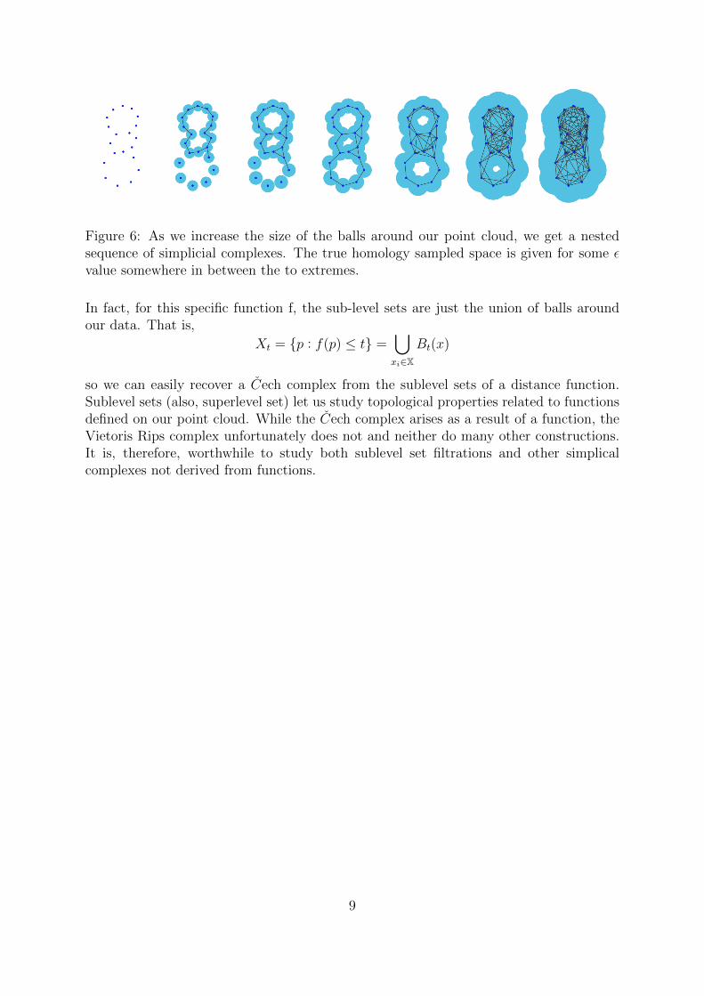
Figure 6: As we increase the size of the balls around our point cloud, we get a nestedsequence of simplicial complexes. The true homology sampled space is given for some εvalue somewhere in between the to extremes.

In fact, for this specific function f, the sub-level sets are just the union of balls aroundour data. That is,

Xt = {p : f(p) ≤ t} =⋃xi∈X

Bt(x)

so we can easily recover a Cech complex from the sublevel sets of a distance function.Sublevel sets (also, superlevel set) let us study topological properties related to functionsdefined on our point cloud. While the Cech complex arises as a result of a function, theVietoris Rips complex unfortunately does not and neither do many other constructions.It is, therefore, worthwhile to study both sublevel set filtrations and other simplicalcomplexes not derived from functions.

9

Topological Persistence

Homology provides us with a language to talk about the structure of a space in a preciseway by associating algebraic structures to topological spaces. Homology describes qual-itative features of the space that are invariant under continuous transformations. Thesefeatures are graded by dimension and are represented by associating homology groupsH0, H1, H2, etc. to each dimension. The rank of H0 measures the number of connectedcomponents of our space. The rank of H1 measures whether loops in the space can becontracted to a single point or not. Similarly, higher dimensional connectivity featurescan be computed and quantified with the use of homology.

Homology and Persistence

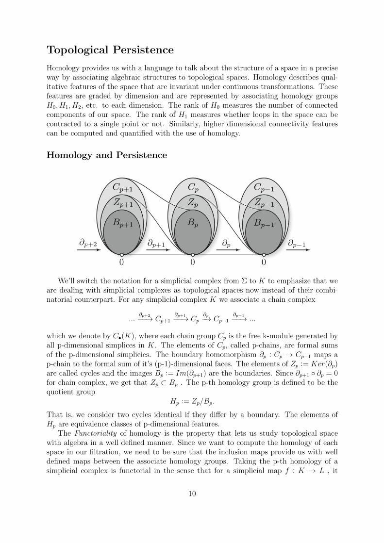
We’ll switch the notation for a simplicial complex from Σ to K to emphasize that weare dealing with simplicial complexes as topological spaces now instead of their combi-natorial counterpart. For any simplicial complex K we associate a chain complex

...∂p+2−−→ Cp+1

∂p+1−−→ Cp∂p−→ Cp−1

∂p−1−−→ ...

which we denote by C•(K), where each chain group Cp is the free k-module generated byall p-dimensional simplices in K. The elements of Cp, called p-chains, are formal sumsof the p-dimensional simplicies. The boundary homomorphism ∂p : Cp → Cp−1 maps ap-chain to the formal sum of it’s (p-1)-dimensional faces. The elements of Zp := Ker(∂p)are called cycles and the images Bp := Im(∂p+1) are the boundaries. Since ∂p+1 ◦ ∂p = 0for chain complex, we get that Zp ⊂ Bp . The p-th homology group is defined to be thequotient group

Hp := Zp/Bp.

That is, we consider two cycles identical if they differ by a boundary. The elements ofHp are equivalence classes of p-dimensional features.

The Functoriality of homology is the property that lets us study topological spacewith algebra in a well defined manner. Since we want to compute the homology of eachspace in our filtration, we need to be sure that the inclusion maps provide us with welldefined maps between the associate homology groups. Taking the p-th homology of asimplicial complex is functorial in the sense that for a simplicial map f : K → L , it

10

induces a linear map C(f) : Cp(K) → Cp(L) for all dimensions p, which defines a maplinear map f∗ : Hp(K) → Hp(L). In other words, a map of spaces defines a map ofhomological features.

To see how homological features change as we filter through different approximations,we apply homology functorially to the filtration to see which features persist the longest.For example, let Kt = Ct(X) be the Cech complex (or any other simplicial complexdescribed above) on a point cloud indexed by t ∈ R≥0. We define K0 := ∅ and defineK := Kt where t is the smallest real number such that if t′ ≥ t then Kt = Kt′ . We obtainthe following filtration

∅ = K0 → ...→ Ki...→ Kt = K.

Because of the functorial properties of associating a chain complex to a simplicial complex,we obtain the sequence

Cp(K0)→ ...→ Cp(Ki)→ ...→ Cp(K).

Computing the p-th homology groups gives us the sequence with induced map

Hp(K0)→ ...Hp(Ki)→ ...→ Hp(K)

This last sequence is an example of a persistence module and we get one for every dimen-sion. Persistence modules are the basic algebraic objects used in the theory of persistenthomology. In categorical terms, if Vec is the category of vector spaces over a fixed fieldand R considered as a total order category (with objects real numbers r ∈ R and mor-phisms ϕ ∈ Hom(r, s) if and only if r ≤ s, then a persistence module can be defined asa functor P : R → Vec . We’ll rigorously define a persistence module in the followingsection.

In our example above, the filtration was indexed by R. Since our data is finite, wewill actually only produce a finite amount of simplicial complexes in our filtration whichdiffer. Therefore, we can index the filtration by N and add a new simplicial complex tothe filtration every time a simplex is added to the construction. Actually, any totallyordered set will give us a persistence module. There is much research in the study multi-dimensional persistence with filtrations indexed by Rn. Despite the seemingly complexprocess of obtaining the persistence module, there are methods to visualize the persistencemodules which make the information attributed to the data set easier to understand.

Barcodes, Diagrams and Landscapes

Our first two visualizations, persistence barcodes and diagrams, are equivalent representa-tions of persistence modules and are sometimes used interchangeably in literature. Theseare what makes persistent homology a useful tool for the every day data analyst sincethey are good visualizations of the topological information we seek. The third repre-sentation, the persistence landscape, comes from the need to incorporate statistics andmachine learning techniques to the theory. The most important theorems in persistenthomology thus far - the structure and stability theorems - can be easily understood withthese representations as well. First, we define the persistence module.

A persistence module is the pair (V , ϕ) where, V = {Vt}t∈R is a family of vector spacesover some k indexed by R, together with linear maps ρt,s : Vs → Vt for every s, t ∈ R such

11

that s ≤ t. These maps must respect the composition in the sense that ρt,r = ρt,s ◦ ρs,r.Again, the definition can be generalized for vector spaces indexed on any totally orderedset as many authors will switch between a finite total order [n] to N or Z.

Structure

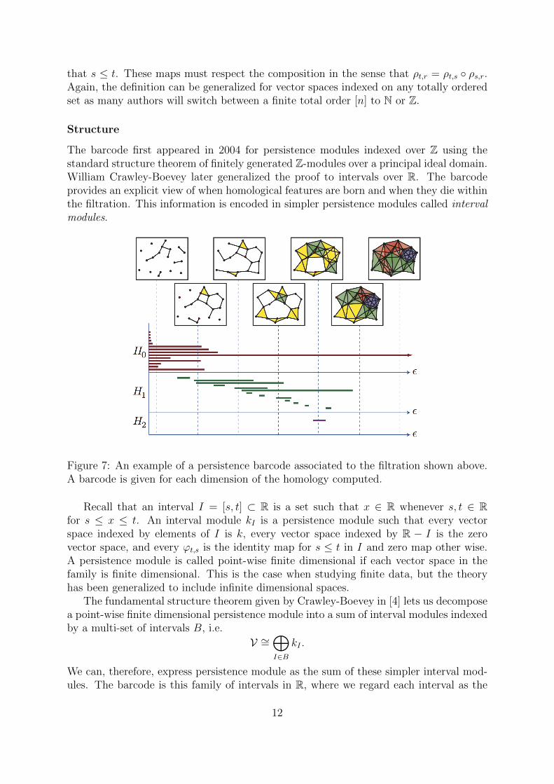
The barcode first appeared in 2004 for persistence modules indexed over Z using thestandard structure theorem of finitely generated Z-modules over a principal ideal domain.William Crawley-Boevey later generalized the proof to intervals over R. The barcodeprovides an explicit view of when homological features are born and when they die withinthe filtration. This information is encoded in simpler persistence modules called intervalmodules.

Figure 7: An example of a persistence barcode associated to the filtration shown above.A barcode is given for each dimension of the homology computed.

Recall that an interval I = [s, t] ⊂ R is a set such that x ∈ R whenever s, t ∈ Rfor s ≤ x ≤ t. An interval module kI is a persistence module such that every vectorspace indexed by elements of I is k, every vector space indexed by R − I is the zerovector space, and every ϕt,s is the identity map for s ≤ t in I and zero map other wise.A persistence module is called point-wise finite dimensional if each vector space in thefamily is finite dimensional. This is the case when studying finite data, but the theoryhas been generalized to include infinite dimensional spaces.

The fundamental structure theorem given by Crawley-Boevey in [4] lets us decomposea point-wise finite dimensional persistence module into a sum of interval modules indexedby a multi-set of intervals B, i.e.

V ∼=⊕I∈B

kI .

We can, therefore, express persistence module as the sum of these simpler interval mod-ules. The barcode is this family of intervals in R, where we regard each interval as the

12

lifespan of a topological feature of the data and the length of the interval determinesa measure of significance of the feature. For each homological dimension we obtain abarcode.

Stability

To have any chance of analyzing noisy data, it is important that persistence modules bestable under small changes in the data. The algebraic stability of persistence theorem, acentral theorem in persistent homology as shown by Chazal et al. in[5], shows exactly.They showed that if there exists a δ-interleaving (a type of isomorphism) between per-sistence modules then there exists a δ-matching (another type of isomorphism) betweentheir corresponding barcodes.

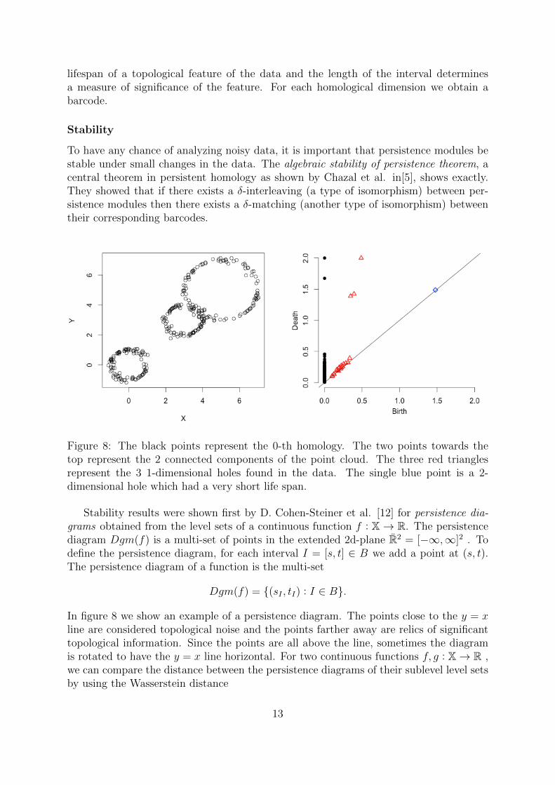
Figure 8: The black points represent the 0-th homology. The two points towards thetop represent the 2 connected components of the point cloud. The three red trianglesrepresent the 3 1-dimensional holes found in the data. The single blue point is a 2-dimensional hole which had a very short life span.

Stability results were shown first by D. Cohen-Steiner et al. [12] for persistence dia-grams obtained from the level sets of a continuous function f : X→ R. The persistencediagram Dgm(f) is a multi-set of points in the extended 2d-plane R2 = [−∞,∞]2 . Todefine the persistence diagram, for each interval I = [s, t] ∈ B we add a point at (s, t).The persistence diagram of a function is the multi-set

Dgm(f) = {(sI , tI) : I ∈ B}.

In figure 8 we show an example of a persistence diagram. The points close to the y = xline are considered topological noise and the points farther away are relics of significanttopological information. Since the points are all above the line, sometimes the diagramis rotated to have the y = x line horizontal. For two continuous functions f, g : X→ R ,we can compare the distance between the persistence diagrams of their sublevel level setsby using the Wasserstein distance

13

Wq(Dgm(f), Dgm(g)) = infγ

(∑

x∈Dgm(f)

‖x− γ(x)‖q∞)1/q

as γ ranges through all possible bijections between multisets, γ : Dgm(f)→ Dgm(g) andwhere ‖x−γ(x)‖∞ = max{|b− b′| ,|d− d′|}. For these definitions to work, one has to addinfinitely many copies of points on the line y = x in the plane. As q goes to infinity, weobtain what is known as the bottleneck distance. Formally, we consider f → Dgm(f),as a map of metric spaces and define stability to be the Lipschitz continuity of the map.We get the stability result

W∞(Dgm(f), Dgm(g)) ≤ ‖f − g‖∞

if functions f and g have finitely many values where the homology changes. The algebraicstability theorem provides a generalization of this result which lets us compare invariantof functions defined on different domains and invariants of filtrations which don’t ariseas level set filtrations such as the Rips complex.

Statistics

To properly be able to use persistent homology for data analysis, we need to address thequality of the diagrams we obtain. We would like to be able to answer the questions:What is the mean of a set of diagrams? Standard deviation? Can we use this to computeconfidence intervals? Unfortunately, the space of persistence diagrams along with the(appropriate) Wasserstein distance gives us a metric space that is not easy to work with.We can define a Frechet mean and variance on the space of persistence diagrams withthis metric but it is not, complete so the mean is not always unique. [6]

We can circumvent this by mapping persistence diagrams or barcodes to differentspace where classical statistics and machine learning techniques can be readily applied.The leading work around to this problem is to consider the persistence landscape of a dataset as defined by Peter Bubenik in his 2012 paper Statistical Topological Data Analysisusing Persistence Landscapes. The persistence landscape is the an injective mapping tothe space of 1-Lipschitz functions. For a point p = (x, y) in some diagram D, we considerthe function

Λp(t) =

t− x+ y t ∈ [x− y, x]

x+ y − t t ∈ (x, x+ y]

0 otherwise

=

t− b t ∈ [b, b+d

2]

d− t t ∈ ( b+d2, d]

0 otherwise.

The persistent landscape of D is a summary of these functions given by

λD(k, t) = kmaxp∈D

Λp(t), t ∈ [0, T ], k ∈ N

where kmax is the k-th largest value in the set. Bubenik showed that there is a stronglaw of large numbers in the space of these landscapes and thus we can compute a uniquemean. However, this mean may fail to be the image of a persistence diagram. In [8],Chazal et al., show that it is possible to define (1 − α)- confidence sets for persistencediagrams as well as confidence bands around persistence landscapes.

14

Since the space of diagrams with the Wasserstein metric isn’t a Hilbert space, it isimpossible to readily employ current machine learning techniques such as PCA or SVM.Nevertheless, the ’kernel trick’ can be used on X to implicitly define a Hilbert space byusing persistence landscapes as is shown in [11]. Whether or not we can find can findother mappings besides the landscape that allow for meaningful results is still an openquestion. The interplay between persistent homology and statistics/machine learning iskey for fully utilizing topological information in data analysis.

15

The TDA package in R

There are many libraries available for computing simplical complexes and persistent ho-mology. These are mostly written mostly in C++ or Java for efficiency. Among thefastest are the libraries DIONYSUS and GUDHI, which can handle simplicies of size upto 1 billion. The statistical programming language R is a popular programming languagefor many data analyst. A group at Carnegie Mellon University has developed a packageTDA available in the CRAN library which provides an R interface to use the algorithmsavailable in the C++ libraries DIONYSUS, GUDHI, and PHAT. [10]For high dimensionaldata, computations should be done on a powerful CPU with more computing power thanan average personal computer. Nevertheless there are still many things that one can dowith smaller data sets. We show a few computations of geometric examples and finallyon real world data sets.

The usual setting in TDA is that we are given a finite point cloud X and assumethat the points in X lives on or ’near’ some object X, usually a compact set, in someambient space Rd. We can mathematically formalize this by using small values of ε forthe Hausdorff distance

dH(X,X) = max{supx∈X

infp∈X‖x− p‖, sup

p∈Xinfx∈X‖p− x‖} = ε.

Torus Data Set

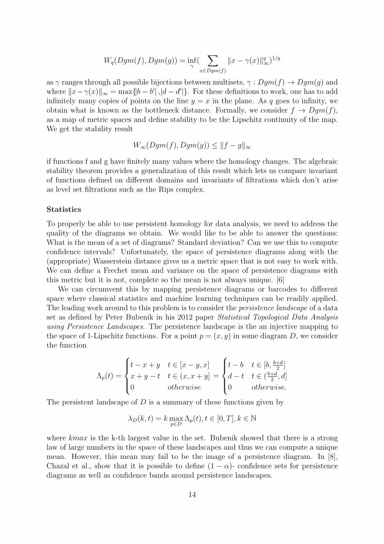
Figure 9: 1000 points sampled from a torus with t he radius from the center of the holeto the center of the torus tube = 4, and radius of torus tube = 2.

Our first data set consists of 1,000 points sampled from a uniform distribution ona torus show in figure 9. Our sample should be dense enough to reflect the features ofthe underlying torus. This example serves is a good reality check as many homologicalfeature are to be detected. Using the function ripsDiag in the package TDA, we can

16

compute the Rips filtration of our point cloud using our choice of either the GUDHI orDIONYSUS libraries. Each library uses a different collection of algorithms to computethe filtration. Algorithms can be significantly faster depending on the size and type ofthe data set. The ripsDiag function with the DIONYSUS algorithm was relatively fasterthan GUDHI in this computation.

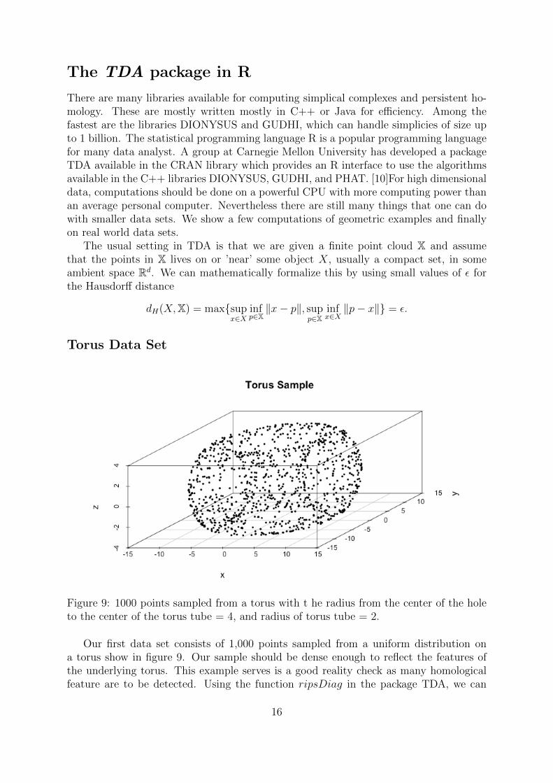
One can clearly see all the homological features of the torus contained in the summariesas shown in figure 10. We use color to help distinguish the homological dimensions. The0th homological dimension tells us that there is one component. The 1st homologicaldimension, as shown in red, shows us the two 1 dimensional loops which are present inthe torus. And finally the blue diamond, and the highest bar, show us the 2-dimensionalvoid that is present in the tube of the torus. The features are clearly separated from thetopological noise which is represented by all the small intervals and points near the y = xline of the diagram.

Figure 10: Barcode and Persistence Diagram for our torus sample

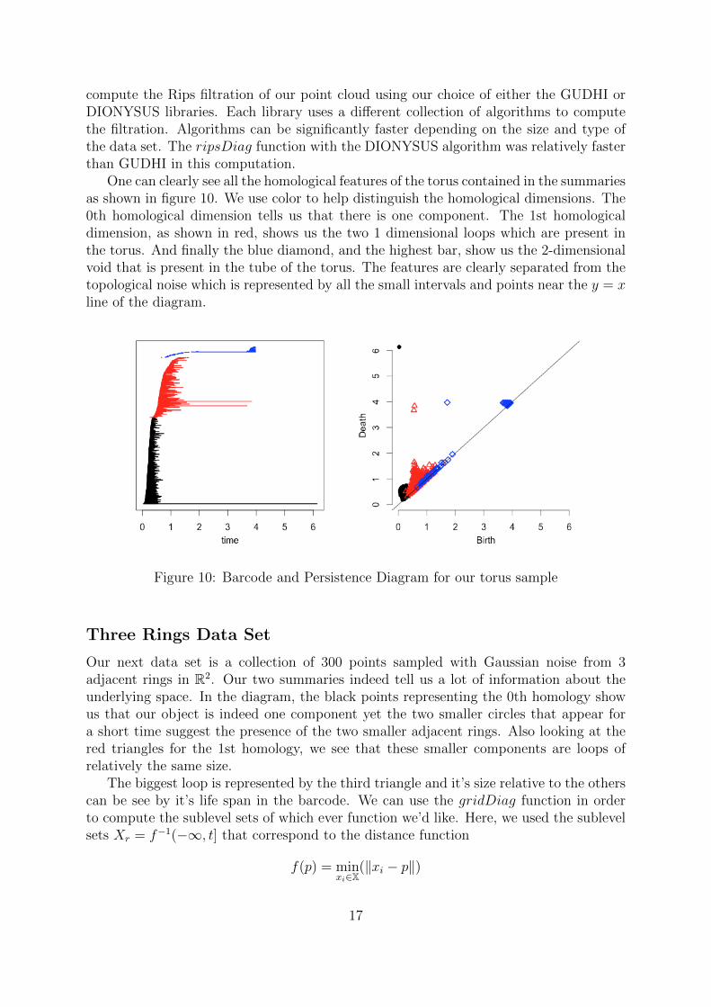
Three Rings Data Set

Our next data set is a collection of 300 points sampled with Gaussian noise from 3adjacent rings in R2. Our two summaries indeed tell us a lot of information about theunderlying space. In the diagram, the black points representing the 0th homology showus that our object is indeed one component yet the two smaller circles that appear fora short time suggest the presence of the two smaller adjacent rings. Also looking at thered triangles for the 1st homology, we see that these smaller components are loops ofrelatively the same size.

The biggest loop is represented by the third triangle and it’s size relative to the otherscan be see by it’s life span in the barcode. We can use the gridDiag function in orderto compute the sublevel sets of which ever function we’d like. Here, we used the sublevelsets Xr = f−1(−∞, t] that correspond to the distance function

f(p) = minxi∈X

(‖xi − p‖)

17

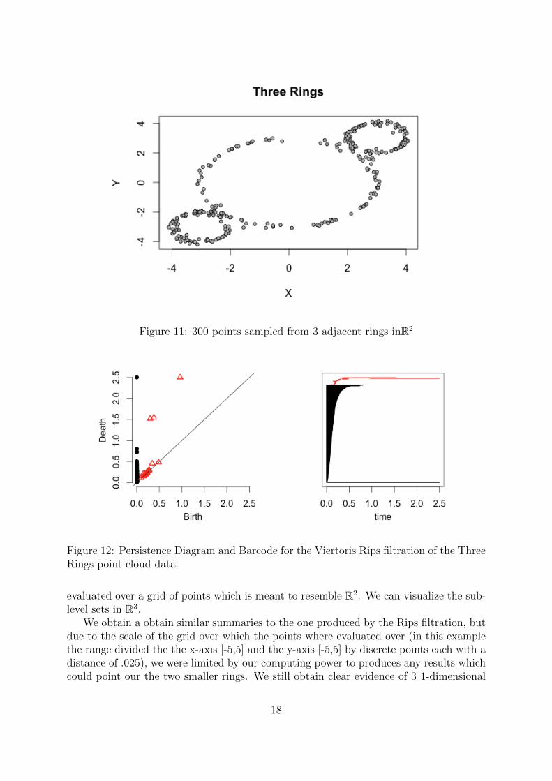
Figure 11: 300 points sampled from 3 adjacent rings inR2

Figure 12: Persistence Diagram and Barcode for the Viertoris Rips filtration of the ThreeRings point cloud data.

evaluated over a grid of points which is meant to resemble R2. We can visualize the sub-level sets in R3.

We obtain a obtain similar summaries to the one produced by the Rips filtration, butdue to the scale of the grid over which the points where evaluated over (in this examplethe range divided the the x-axis [-5,5] and the y-axis [-5,5] by discrete points each with adistance of .025), we were limited by our computing power to produces any results whichcould point our the two smaller rings. We still obtain clear evidence of 3 1-dimensional

18

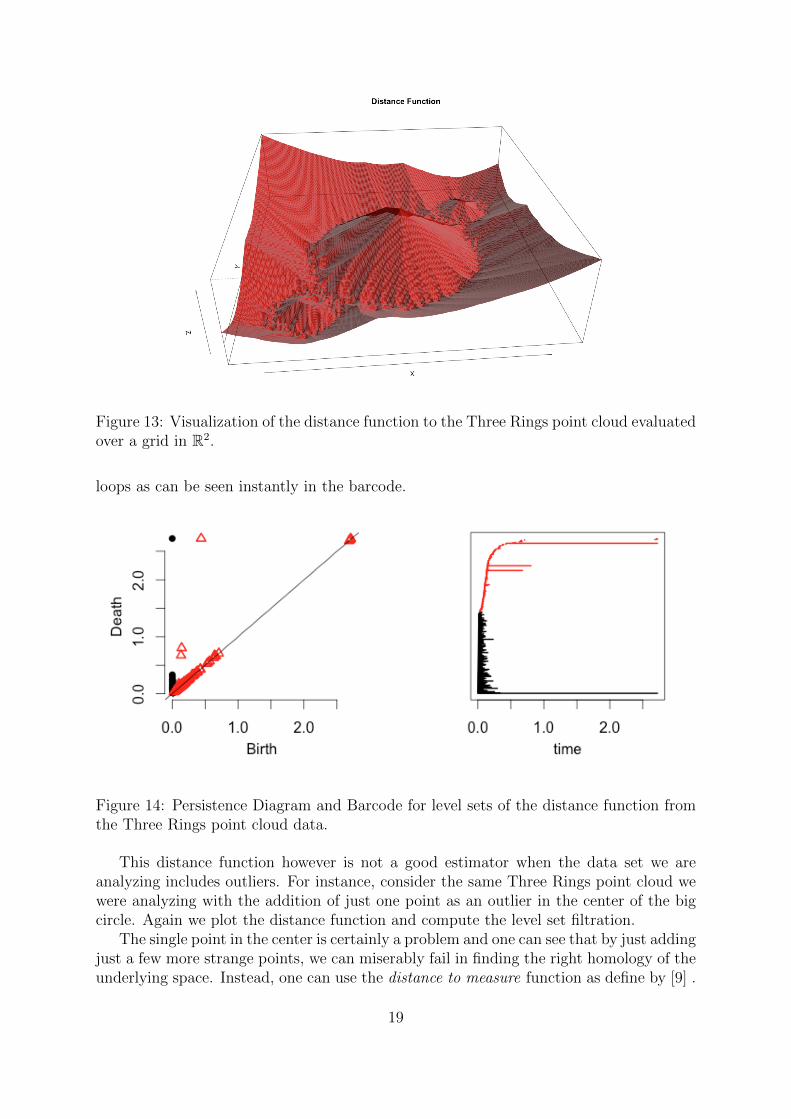
Figure 13: Visualization of the distance function to the Three Rings point cloud evaluatedover a grid in R2.

loops as can be seen instantly in the barcode.

Figure 14: Persistence Diagram and Barcode for level sets of the distance function fromthe Three Rings point cloud data.

This distance function however is not a good estimator when the data set we areanalyzing includes outliers. For instance, consider the same Three Rings point cloud wewere analyzing with the addition of just one point as an outlier in the center of the bigcircle. Again we plot the distance function and compute the level set filtration.

The single point in the center is certainly a problem and one can see that by just addingjust a few more strange points, we can miserably fail in finding the right homology of theunderlying space. Instead, one can use the distance to measure function as define by [9] .

19

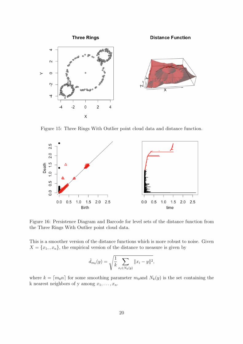
Figure 15: Three Rings With Outlier point cloud data and distance function.

Figure 16: Persistence Diagram and Barcode for level sets of the distance function fromthe Three Rings With Outlier point cloud data.

This is a smoother version of the distance functions which is more robust to noise. GivenX = {x1, , xn}, the empirical version of the distance to measure is given by

dm0(y) =

√1

k

∑xi∈Nk(y)

‖xi − y‖2,

where k = dm0ne for some smoothing parameter m0and Nk(y) is the set containing thek nearest neighbors of y among x1, . . . , xn.

20

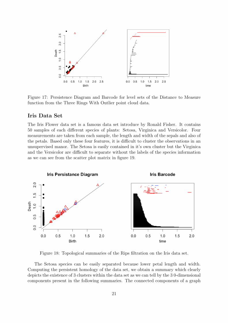
Figure 17: Persistence Diagram and Barcode for level sets of the Distance to Measurefunction from the Three Rings With Outlier point cloud data.

Iris Data Set

The Iris Flower data set is a famous data set introduce by Ronald Fisher. It contains50 samples of each different species of plants: Setosa, Virginica and Versicolor. Fourmeasurements are taken from each sample, the length and width of the sepals and also ofthe petals. Based only these four features, it is difficult to cluster the observations in anunsupervised manor. The Setosa is easily contained in it’s own cluster but the Virginicaand the Versicolor are difficult to separate without the labels of the species informationas we can see from the scatter plot matrix in figure 19.

Figure 18: Topological summaries of the Rips filtration on the Iris data set.

The Setosa species can be easily separated because lower petal length and width.Computing the persistent homology of the data set, we obtain a summary which clearlydepicts the existence of 3 clusters within the data set as we can tell by the 3 0-dimensionalcomponents present in the following summaries. The connected components of a graph

21

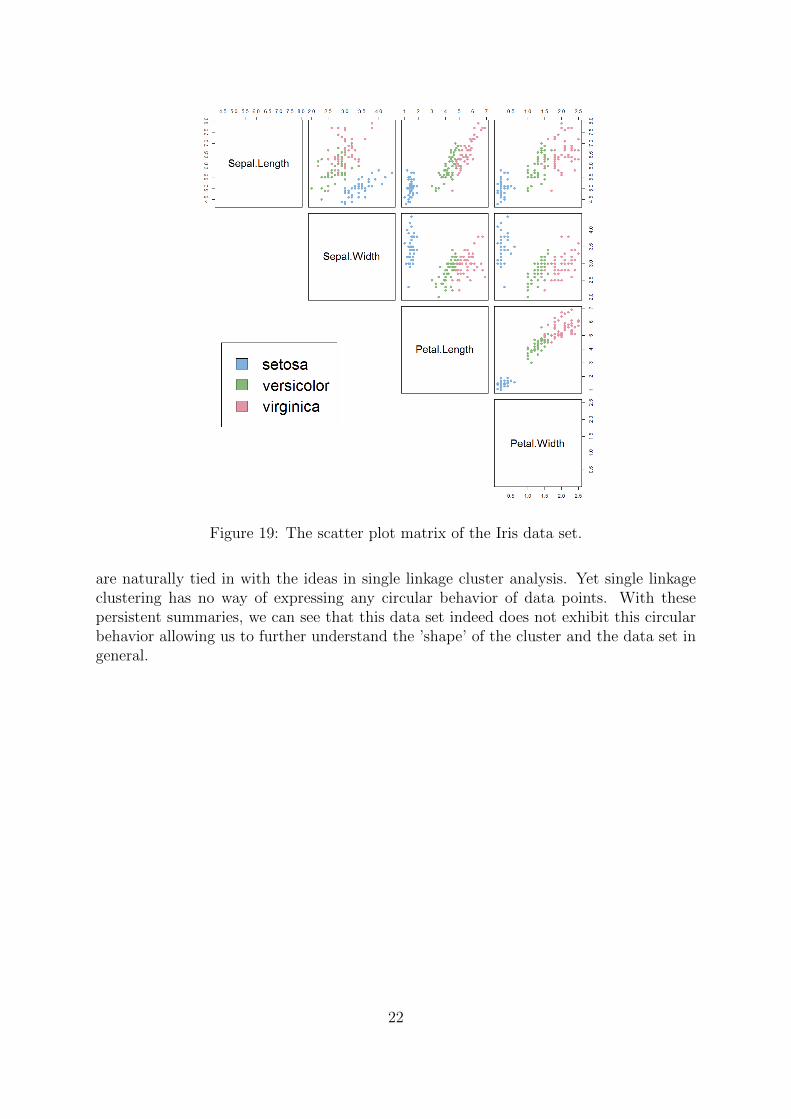
Figure 19: The scatter plot matrix of the Iris data set.

are naturally tied in with the ideas in single linkage cluster analysis. Yet single linkageclustering has no way of expressing any circular behavior of data points. With thesepersistent summaries, we can see that this data set indeed does not exhibit this circularbehavior allowing us to further understand the ’shape’ of the cluster and the data set ingeneral.

22

Discussion

Persistent homology is an exciting new idea for modern mathematics and data analysis.In this paper we have shown how one can combinatorially encode the similarity of pointswithin a data set and use this information to study the underlying topological propertiesof the data set. The topological properties of a data set become useful when trying tounderstand the intrinsic structure of the space from which the data is being sampledfrom. Qualitative information, such as homology, provides insight to the data set whichis key for further exploration and analysis. The rich theory of persistence has manyfurther directions to explore. Popular one being multidimensional persistence and zig-zagpersistence which considers, instead of a filtration where functions only go ’to the right’,functions in either direction. Persistence is being studied not only in an applied sense buttheoretical as well. The development of the theory of persistent homology, along with thenecessary integration of statistics and machine learning, will hopefully continue to showthe benefits of topological information in data analysis as researchers and practitionersalike delve deep into the new field of topological data analysis.

References

[1] Michel Verleysen and Damien Franois. The Curse of Dimensionality in Data Miningand Time Series Prediction. IW ANN 2005, LNCS 3512, pp. 758 770, 2005. Springer-Verlag Berlin Heidelberg 2005.

[2] Carlsson, G (2009). Topology and Data. Bull. Amer. Math. Soc. 46, 255-308.

[3] Peter Bubenik, Vin de Silva, and Jonathan Scott. Metrics for generalizedpersistence modules. Foundations of Computational Mathematics, pages 131.http://arxiv.org/abs/1312.3829.

[4] William Crawley-Boevey Decomposition of pointwise finite-dimensional persistencemodules. arXiv:1210.0819 [math.RT]

[5] Frederic Chazal, Vin de Silva, Marc Glisse, and Steve Oudot. The structure andstability of persistence modules. arXiv:1207.3674 [math.AT]

[6] Brittany Terese Fasy, Fabrizio Lecci, Alessandro Rinaldo, Larry Wasserman, Sivara-man Balakrishnan, Aarti Singh. Confidence sets for persistence diagrams Ann. Statist.Volume 42, Number 6 (2014), 2301-2339.

[7] Edelsbrunner, Herbert; Kirkpatrick, David G.; Seidel, Raimund (1983), On the shapeof a set of points in the plane IEEE Transactions on Information Theory 29 (4):551559, doi:10.1109/TIT.1983.1056714

[8] Frederic Chazal, Brittany Terese Fasy, Fabrizio Lecci, Alessandro Rinaldo, AartiSingh, and Larry Wasserman. On the Bootstrap for Persistence Diagrams and Land-scapes. arxiv:1311.0376.

23

[9] Frdric Chazal, Brittany T. Fasy, Fabrizio Lecci, Bertrand Michel, Alessandro Rinaldo,Larry Wasserman. Robust Topological Inference: Distance To a Measure and KernelDistance arXiv:1412.7917 [cs.MS]

[10] Brittany Terese Fasy, Jisu Kim, Fabrizio Lecci, Clment Maria. Introduction to the Rpackage TDA, arXiv:1411.1830 [cs.MS]

[11] Jan Reininghaus, Stefan Huber, Ulrich Bauer, Roland Kwitt A Stable Multi-ScaleKernel for Topological Machine Learning http://arxiv.org/pdf/1412.6821.pdf

[12] D. Cohen-Steiner, H. Edelsbrunner, and J. Harer. Stability of persistence diagrams.Discrete and Computational Geometry, 37(1):103120, 2007.

24