Topological data analysis(TDA) for functional connectivity: Persistence vineyard approach for brain dynamics

Presenter: Jaejun Yoo

The Brain – A complex network

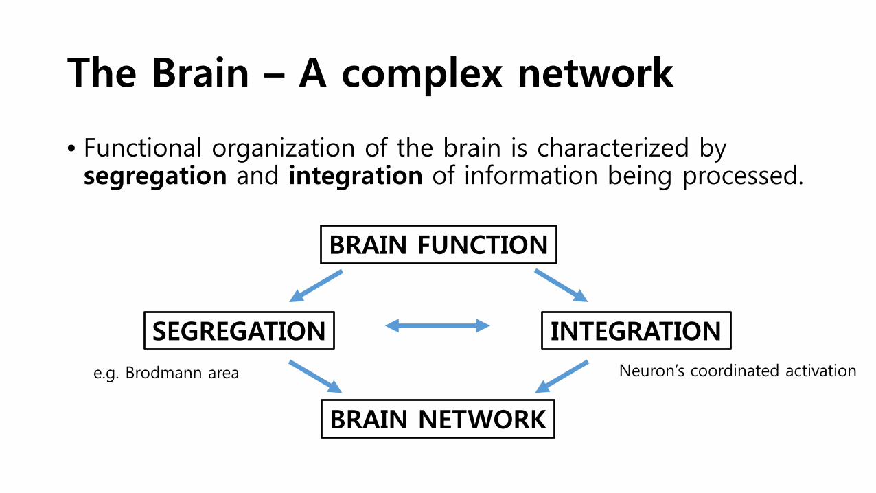
• Functional organization of the brain is characterized by segregation and integration of information being processed.

BRAIN FUNCTION

BRAIN NETWORK

SEGREGATION INTEGRATIONe.g. Brodmann area Neuron’s coordinated activation

Functional Connectivity

• Temporal dependency of neural activation patterns of anatomically separated brain regions.

• It reflects statistical dependencies between distinct and distant regions of information processing neuronal populations, e.g. correlation, covariance, spectral coherence, or phase locking.

• Deduced from neuroimaging modalities like fMRI, EEG, MEG, PET, and SPECT.

Buckner et al, 2013

Dynamic Functional Connectivity

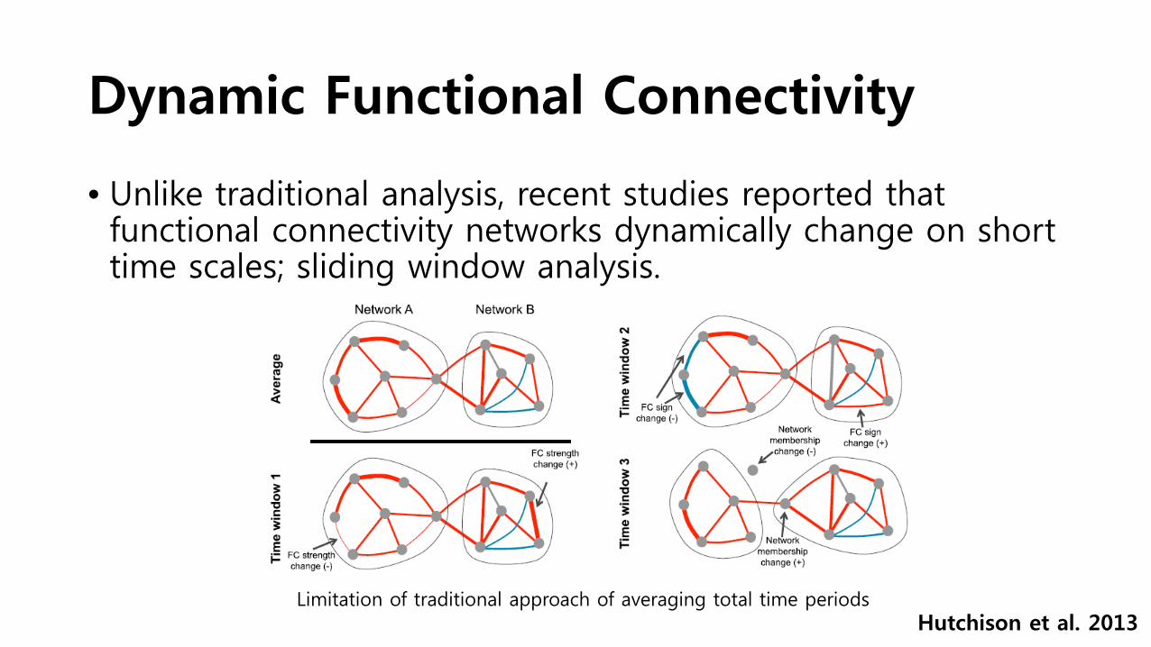
• Unlike traditional analysis, recent studies reported that functional connectivity networks dynamically change on short time scales; sliding window analysis.

Limitation of traditional approach of averaging total time periodsHutchison et al. 2013

Computational Methods to Quantify FC

• Two broad classes of the computational methods

Knowledge-basedSupervised

(e.g SPM based on GLM and GRF)

Data-drivenExplanatory

Unsupervised(e.g Decomposition, clustering)

Buckner et al, 2013 PCA ICABritz et al 2010

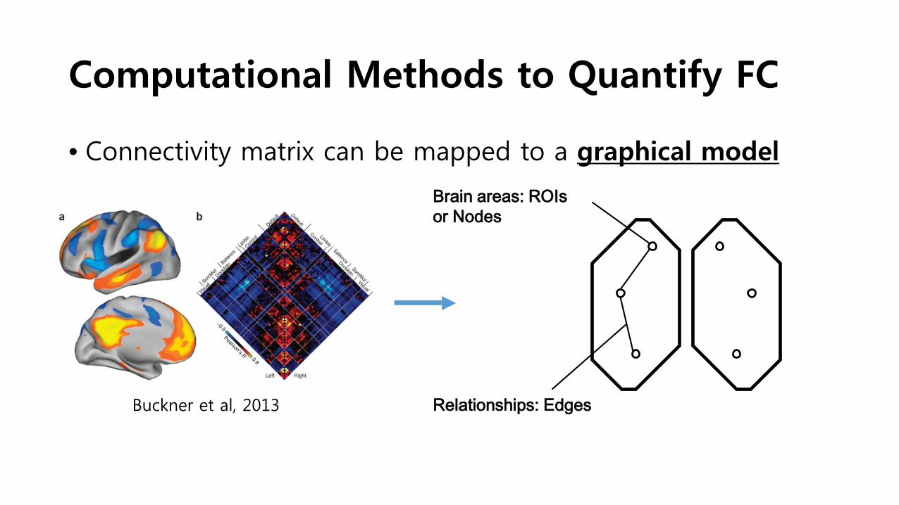
• Connectivity matrix can be mapped to a graphical model

Buckner et al, 2013

Brain areas: ROIs or Nodes

Relationships: Edges

Computational Methods to Quantify FC

Computational Methods to Quantify FC

Heuvel and Sporns 2013

SegregationClustering

IntegrationDistancePath Length

InfluenceDegreeCentrality (Hubs)

Computational Methods to Quantify FC

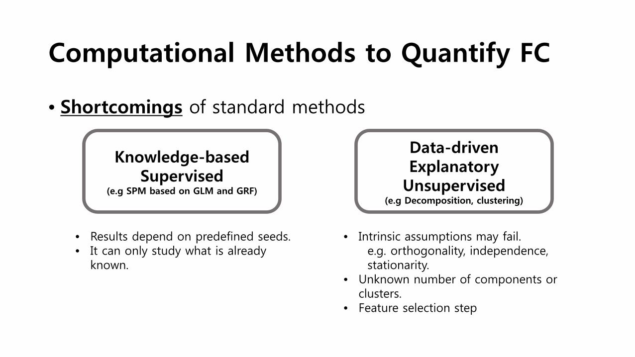
• Results depend on predefined seeds.• It can only study what is already

known.

• Intrinsic assumptions may fail.e.g. orthogonality, independence, stationarity.

• Unknown number of components or clusters.

• Feature selection step

• Shortcomings of standard methods

Knowledge-basedSupervised

(e.g SPM based on GLM and GRF)

Data-drivenExplanatory

Unsupervised(e.g Decomposition, clustering)

Computational Methods to Quantify FC

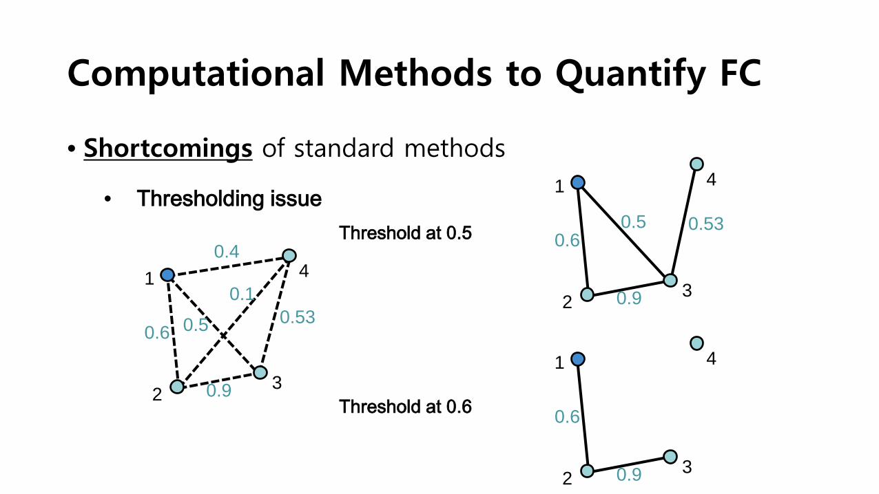
• Shortcomings of standard methods

1

2 3

40.4

0.6

0.9

0.10.530.5

1

2 3

4

0.6

0.9

0.5Threshold at 0.5

1

2 3

4

0.6

0.9

Threshold at 0.6

0.53• Thresholding issue

Computational Methods to Quantify FC

• Shortcomings of standard methods

• Thresholding issue• Data perturbation across …

1/f spectral distribution, subject by subject, condition to condition, …

1/f noise – Scholarpedia, Brunet et al 2011

Topological Data Analysis

• Data-Driven Approach• Studying complex high dimensional data without any assumptions or feature selections

• Shape has Meaning; extracting shapes(patterns) of data• Qualitative and quantitative summaries of the data are provided.

• Especially, TDA using PERSISTENT HOMOLOGY provides threshold-free analysis.

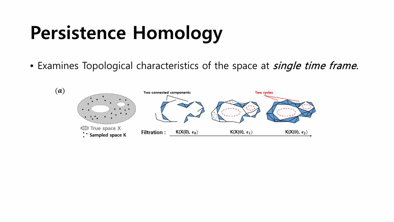
Persistence Homology

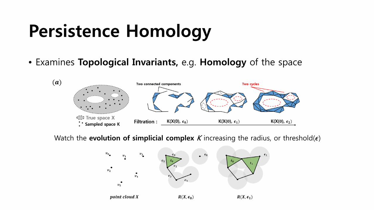
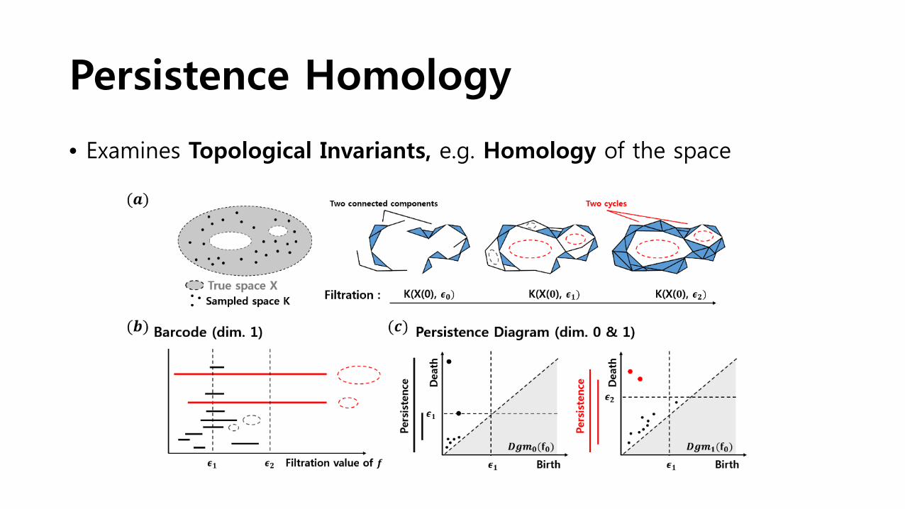
• Examines Topological Invariants, e.g. Homology of the space

Watch the evolution of simplicial complex K increasing the radius, or threshold(𝝐𝝐)

Persistence Homology

• Examines Topological Invariants, e.g. Homology of the space

Values of simplexes(nodes, edges, and faces) are determined by a height function 𝑓𝑓: 𝑲𝑲 → ℝand an order sequence of complexes is constructed,

Persistence Homology

• Examines Topological Invariants, e.g. Homology of the space

Exemplary application: fMRI data

• Mouse forepaw stimulation, fMRI (full vs. 2X down sampled)

• Dimension: 64 by 64 by 150 (time)

• Distance was calculated by the correlation with their hemodynamic response function

10 20 30 40 50 60

10

20

30

40

50

60

Data(X)

Time→

X(i, :)

𝑖𝑖 𝑡𝑡𝑡 voxeltime-series

adja

cency

val

ue

voxel→

voxel→

voxel→

PairwiseDistance Matrix𝐃𝐃𝐃𝐃𝐃𝐃𝐃𝐃 𝐕𝐕𝐕𝐕𝐕𝐕𝐕𝐕𝐕𝐕 𝐃𝐃 ,𝐕𝐕𝐕𝐕𝐕𝐕𝐕𝐕𝐕𝐕 𝐣𝐣 =

| 𝟏𝟏 − 𝒂𝒂𝒂𝒂𝒂𝒂 𝒊𝒊 − {𝟏𝟏 − 𝒂𝒂𝒂𝒂𝒂𝒂(𝒂𝒂)}|

voxel→

𝐚𝐚𝐚𝐚𝐣𝐣 = 𝐚𝐚𝐚𝐚𝐃𝐃(𝐜𝐜𝐕𝐕𝐜𝐜𝐜𝐜(𝐗𝐗(𝐃𝐃, : ),𝐡𝐡𝐜𝐜𝐡𝐡)

Schematic flow of distance matrix calculation

Result

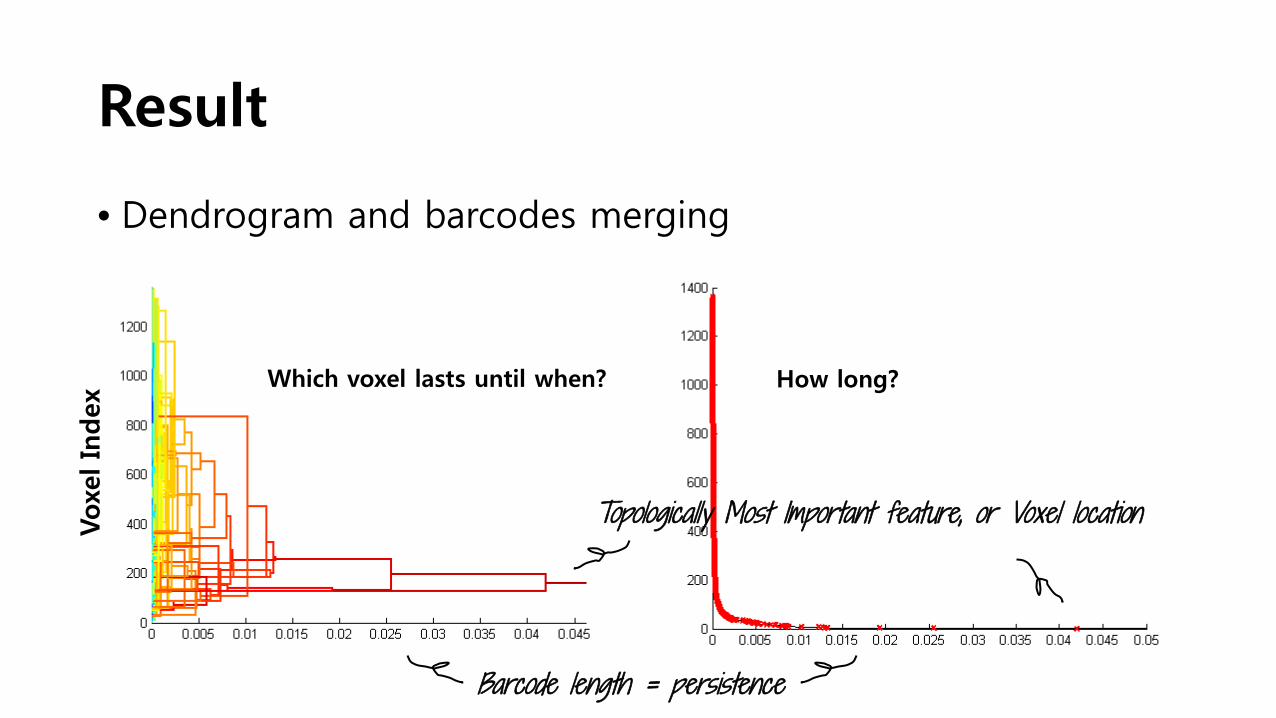
• Dendrogram and barcodes merging

Barcode length = persistence

Topologically Most Important feature, or Voxel locationVoxe

l In

dex

Which voxel lasts until when? How long?

ResultfMRI full data

ResultfMRI Down sampled 2X data

Result

fMRI full

fMRI down 2X

NOTE THAT…

• No t-test relying on p-value selection was performed.

• Quantified criteria of topological importance of the features are provided.

TO FURTHER ASSESS DYNAMICSOF FUNCTIONAL CONNECTIVITY…

Persistence Vineyard

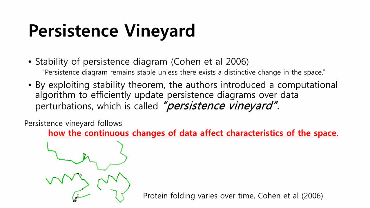
• Stability of persistence diagram (Cohen et al 2006)“Persistence diagram remains stable unless there exists a distinctive change in the space.”

• By exploiting stability theorem, the authors introduced a computational algorithm to efficiently update persistence diagrams over data perturbations, which is called “persistence vineyard”.

Persistence vineyard follows how the continuous changes of data affect characteristics of the space.

Protein folding varies over time, Cohen et al (2006)

Persistence Homology

• Examines Topological characteristics of the space at single time frame.

Persistence Homology

• Examines Topological characteristics of the space at single time frame.

Extend the persistent homology analysis toward the 3rd dimension:“temporal domain”, “Examine the variation over multiple time frame”

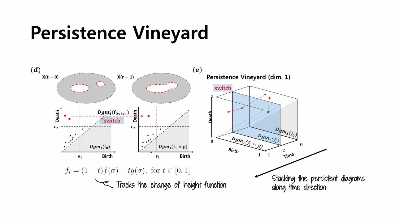
Persistence Vineyard

Stacking the persistent diagrams along time directionTracks the change of height function

Application: EEG data

Normal Subjects, resting and gaming alternatively• EEG, 8 channel,

• Sampling rate: 512 Hz

• Sliding window analysis

• window length: 30 s / shifting length : 2 s (2m 30 s = 31 frame)

• Delta (0.3-4 Hz), Theta (4-8 Hz), Alpha (8-13 Hz), Beta (13-30 Hz)

• ICA, Epoch rejection performed

G3 R3G1RR G2R1 R2

5 min 5 min 5 min5 min5 min5 min5 min

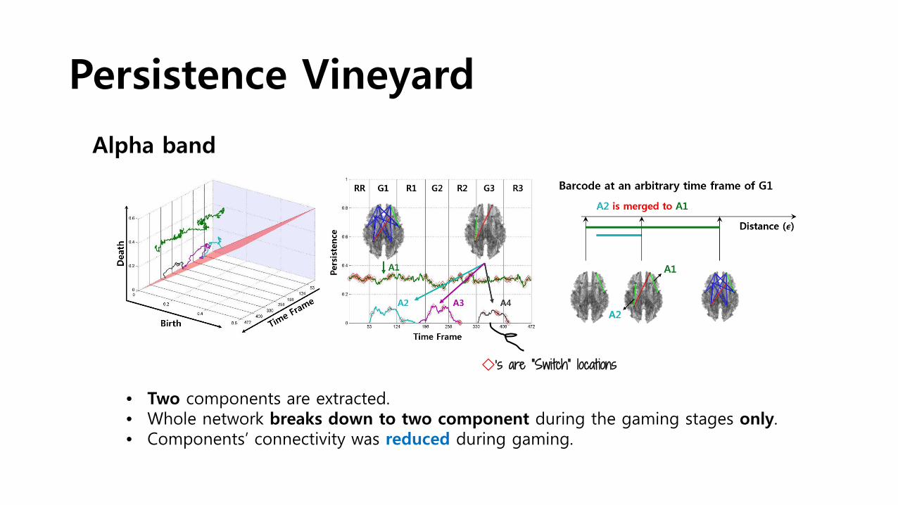
Persistence Vineyard

Alpha band

◇’s are “Switch” locations

• Two components are extracted.• Whole network breaks down to two component during the gaming stages only.• Components’ connectivity was reduced during gaming.

Persistence Vineyard

Beta band

• Four components are extracted.• Components exist in hierarchical way residing in different strengths.• Components’ connectivity was enhanced during gaming.

◇’s are “Switch” locations

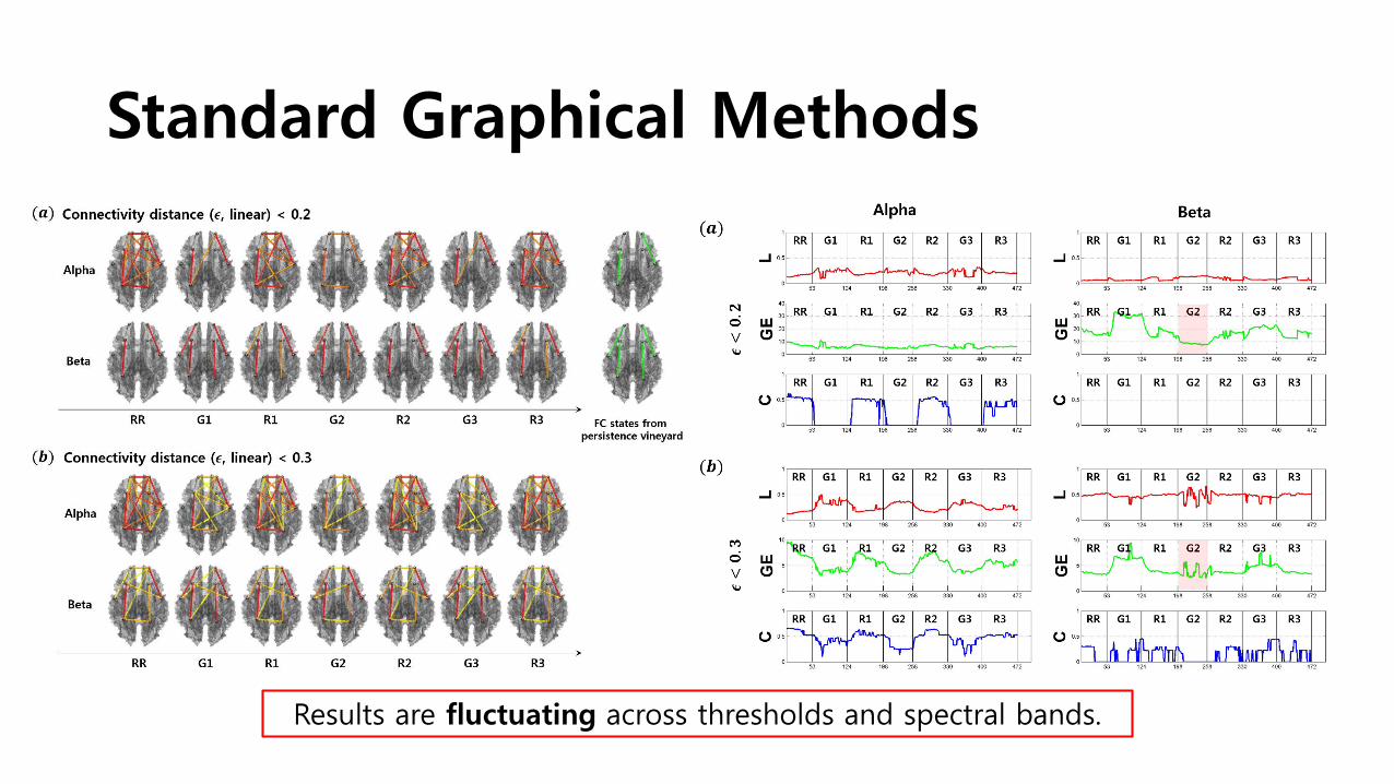
Standard Graphical Methods

Results are fluctuating across thresholds and spectral bands.

• Comparison with the vineyard generated under null hypothesis (randomly shuffled in time order)

• No significant structure or consistent pattern was found

• Number of SWITCH soared

Advantages of Persistence Vineyard• Retain the advantages of TDA and persistent homology;

e.g. Data-driven, threshold-free, assumption-free approach. Do not require feature selection (features and their are determined by the data).

• Good properties with mathematical background.• Provide quantified summaries of network variation• Displayed consistent results with the previous EEG studies.

Alpha : restingBeta : attention, task-related

[SUMMARY]