1

Topics in Astrophysics: Module 2

Michaelmas Term, 2010: Prof Craig Mackay

Module 2:• Magnitudes, HR diagrams, Distance determination, • The Sun as a typical star (timescales, internal temperature and pressure, energy source).• Stellar lifecycles• Newtonian mechanics, Orbits, Tides• Blackbody radiation, Planck’s, Wein’s and Stephan-Boltzman’s laws• What makes things glow: Continuum radiation mechanisms, emission line mechanisms, spectra.

2

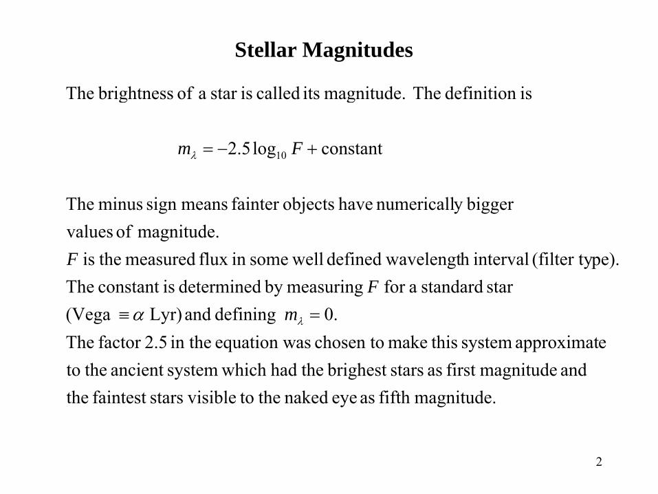
Stellar Magnitudes

magnitude.fifth as eye naked the to visiblestarsfaintest theand magnitudefirst as starsbrighest thehad which systemancient theto

eapproximat system thismake chosen to asequation w in the 2.5factor The.0 defining and Lyr) (Vega

star standard afor measuringby determined isconstant Thepe).(filter ty intervalh wavelengtdefined wellsomein flux measured theis

magnitude. of valuesbiggery numericall have objectsfainter meanssign minus The

constant log5.2

isdefinitionThe magnitude.itscalledisstar aofbrightnessThe

10

=≡

+−=

λ

λ

α mF

F

Fm

3

Apparent magnitudes

diagram.colour -colour ausing measured becan reddening distance same at the all arewhich

stars ofcluster aFor reddened. islight themore affected are swavelengthshort Because fainter. seemstar a make sight will of line thealongDust

c.logarithmi are magnitudes because ratiosflux course of are colours Theseor

e.g. ts.measuremen magnitude 2between difference theby taking obtained becan star a ofcolour theof measureA

LK, H, J, z, I, R, V, B, U,are system CousinsJohnson in the magnitudes The

passband. the torefersch letter whi a as written are magnitudesApparent

VBBU −−

4

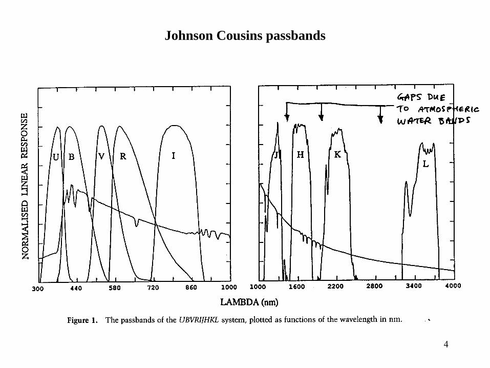
Johnson Cousins passbands

5

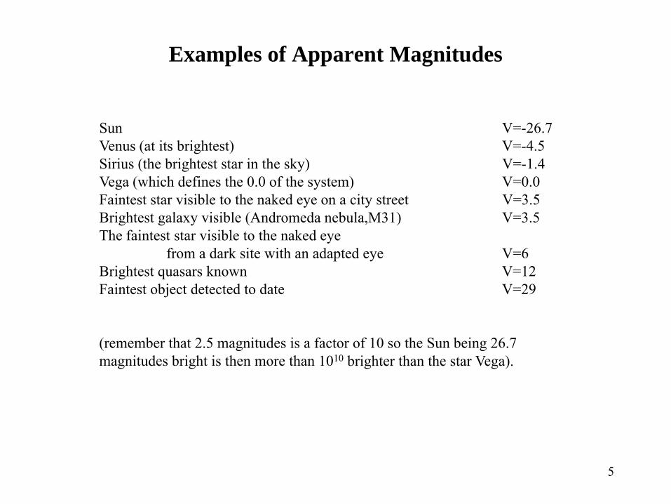
Examples of Apparent Magnitudes

Sun V=-26.7Venus (at its brightest) V=-4.5Sirius (the brightest star in the sky) V=-1.4Vega (which defines the 0.0 of the system) V=0.0Faintest star visible to the naked eye on a city street V=3.5Brightest galaxy visible (Andromeda nebula,M31) V=3.5The faintest star visible to the naked eye

from a dark site with an adapted eye V=6Brightest quasars known V=12Faintest object detected to date V=29

(remember that 2.5 magnitudes is a factor of 10 so the Sun being 26.7 magnitudes bright is then more than 1010 brighter than the star Vega).

6

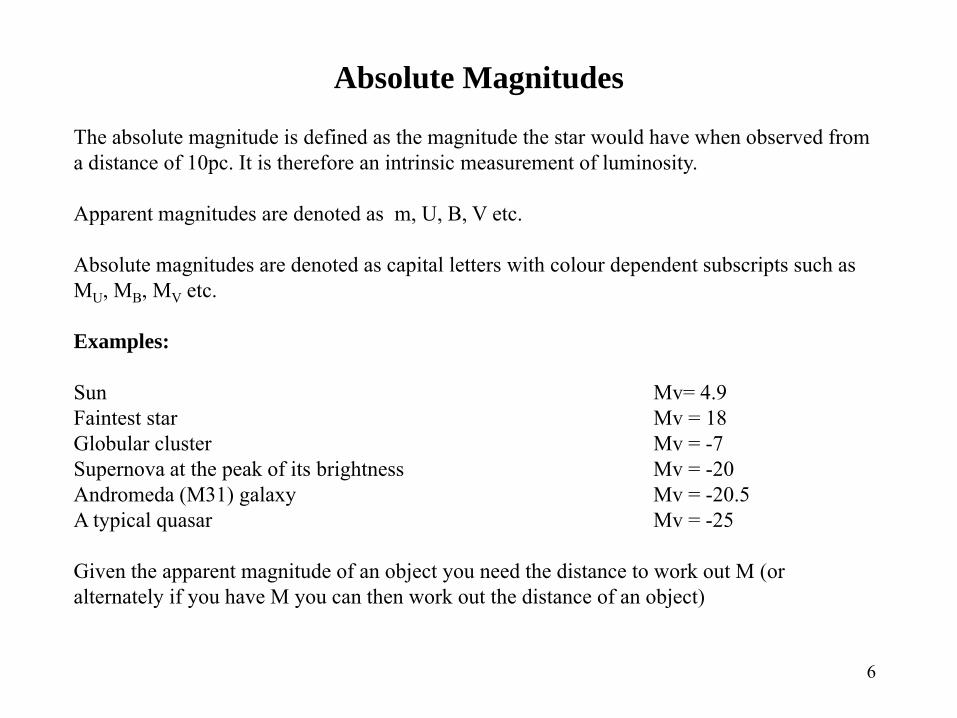
Absolute Magnitudes

The absolute magnitude is defined as the magnitude the star would have when observed from a distance of 10pc. It is therefore an intrinsic measurement of luminosity.

Apparent magnitudes are denoted as m, U, B, V etc.

Absolute magnitudes are denoted as capital letters with colour dependent subscripts such as MU, MB, MV etc.

Examples:

Sun Mv= 4.9Faintest star Mv = 18Globular cluster Mv = -7Supernova at the peak of its brightness Mv = -20Andromeda (M31) galaxy Mv = -20.5A typical quasar Mv = -25

Given the apparent magnitude of an object you need the distance to work out M (or alternately if you have M you can then work out the distance of an object)

7

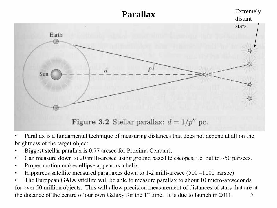
Parallax

• Parallax is a fundamental technique of measuring distances that does not depend at all on the brightness of the target object.• Biggest stellar parallax is 0.77 arcsec for Proxima Centauri.• Can measure down to 20 milli-arcsec using ground based telescopes, i.e. out to ~50 parsecs.• Proper motion makes ellipse appear as a helix• Hipparcos satellite measured parallaxes down to 1-2 milli-arcsec (500 –1000 parsec)• The European GAIA satellite will be able to measure parallax to about 10 micro-arcseconds for over 50 million objects. This will allow precision measurement of distances of stars that are at the distance of the centre of our own Galaxy for the 1st time. It is due to launch in 2011.

Extremelydistantstars

8

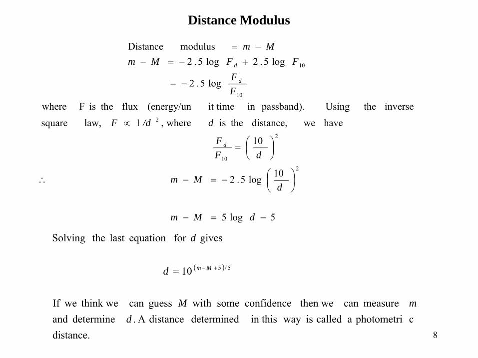
Distance Modulus

5log5

10log5.2

10

have wedistance, theis where,1 law, squareinverse the Usingpassband).in it time(energy/unflux theis F where

log5.2

log5.2log5.2 modulus Distance

2

2

10

2

10

10

−=−

⎟⎠⎞

⎜⎝⎛−=−∴

⎟⎠⎞

⎜⎝⎛=

∝

−=

+−=−−=

dMm

dMm

dFF

d/dF

FF

FFMmMm

d

d

d

( )

distance.cphotometri a called is way in this determined distanceA . determine and

measurecan then weconfidence some with guesscan think we weIf

10

givesfor equation last theSolving

5/5

dmM

d

d

Mm +−=

9

How do we estimate absolute mag M

• For stars observed by the astrometric satellite Hipparcos we know d so we can get M → standard candles

• More standard candles can be established by association with the Hipparcos ones.• Some standard candles can be several steps removed from a geometric distance

determination.

Examples of Standard Candles

• Nearby stars of known type• Main Sequence in the HR diagram• Cepheid Variable stars• RR Lyrae Variable stars• Supernovae

• The problem is that none of these genuinely and totally are standard candles: they are only an approximation to one and therefore we have to be very careful that we understand the limitations implicit in using each of these so-called standard candles

10

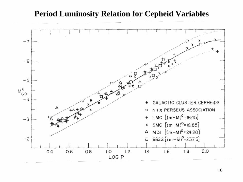
Period Luminosity Relation for Cepheid Variables

11

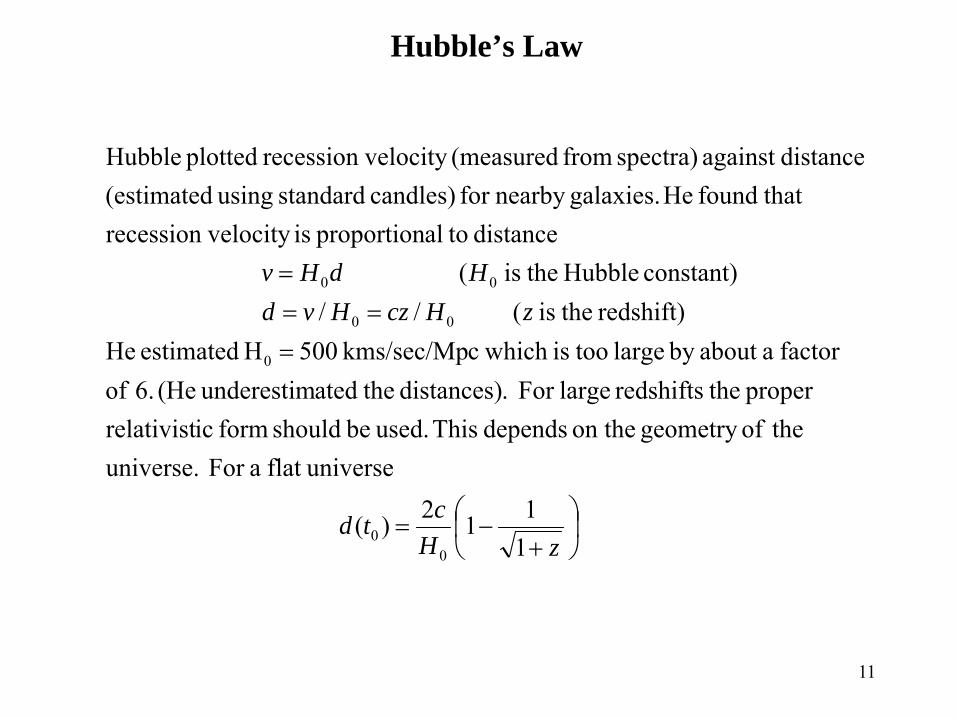
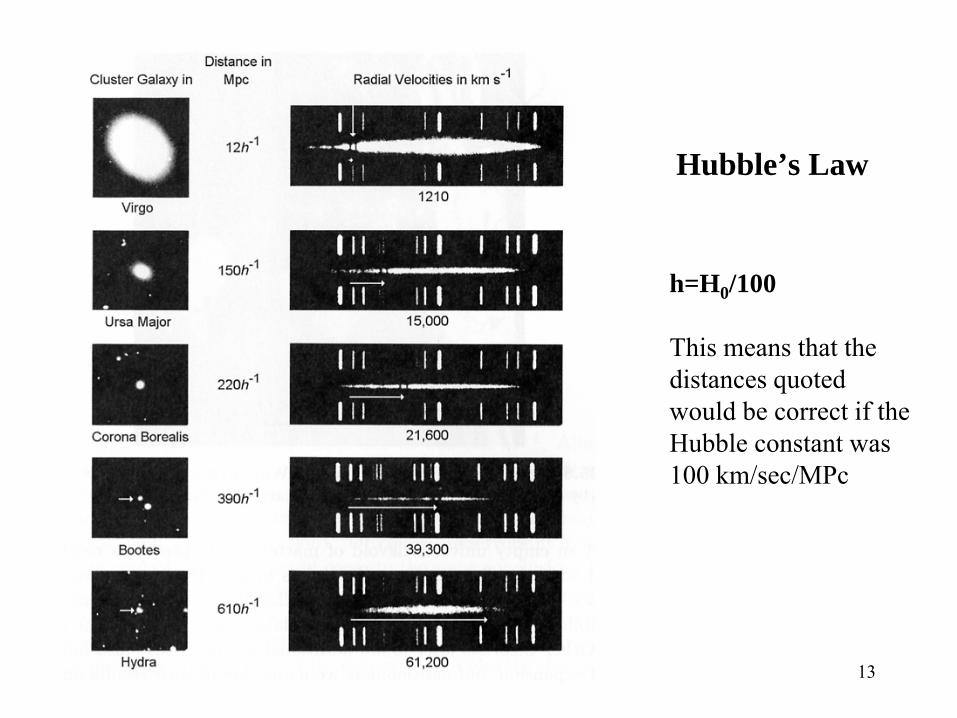
Hubble’s Law

⎟⎠

⎞⎜⎝

⎛+

−=

===

=

zHctd

zHczHvdHdHv

1112)(

universeflat aFor universe. theofgeometry on the depends This used. be should form icrelativist

proper theredshifts largeFor .distances) theatedunderestim (He 6. offactor aabout by large toois which ckms/sec/Mp 500H estimated He

redshift) theis ( //constant) Hubble theis (

distance toalproportion isvelocity recession thatfound He galaxies.nearby for candles) standard using (estimated

distanceagainst spectra) from (measuredvelocity recession plotted Hubble

00

0

00

00

12

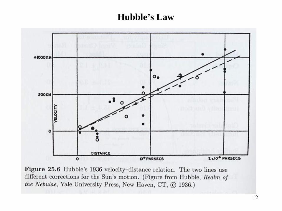
Hubble’s Law

13

Hubble’s Law

h=H0/100

This means that the distances quoted would be correct if the Hubble constant was 100 km/sec/MPc

14

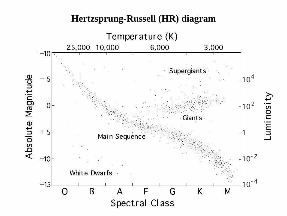
Hertzsprung-Russell (HR) diagram

• This is a plot of stellar surface temperature against stellar luminosity. • Temperature is plotted on the x axis with the coolest values to the right. Both axes are

logarithmic.• Values may come either from observations or theory.• A point represents a single star.• An evolutionary track represents the way a single star evolves with time.• An isochrone represents a sequence of stellar models of different masses but all with

the same age (and initial composition).

How do we measure temperature?

• From spectral type (class) – relative line strengths strongly dependant on temperature.• From apparent magnitudes – colours such as U-B and B-V have a well defined

dependence on temperature. These quantities are essentially flux ratios because magnitudes are logarithmic.

15

Hertzsprung-Russell (HR) diagram

16

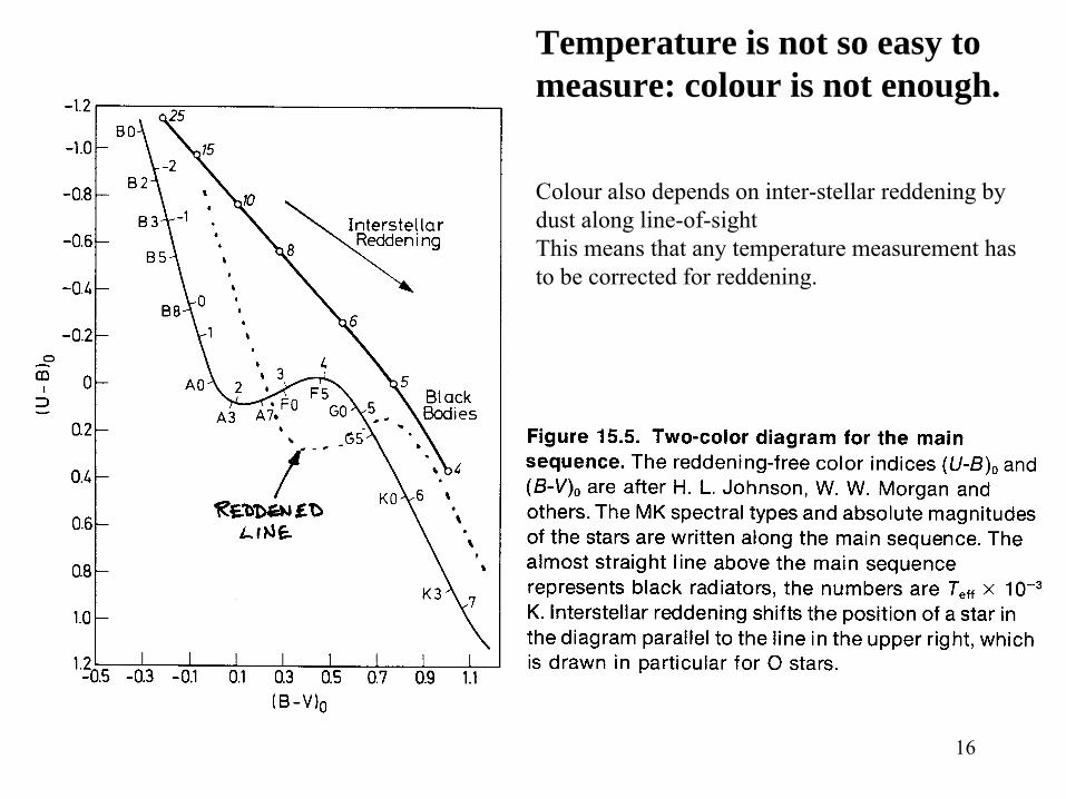
Temperature is not so easy to measure: colour is not enough.

Colour also depends on inter-stellar reddening by dust along line-of-sightThis means that any temperature measurement has to be corrected for reddening.

17

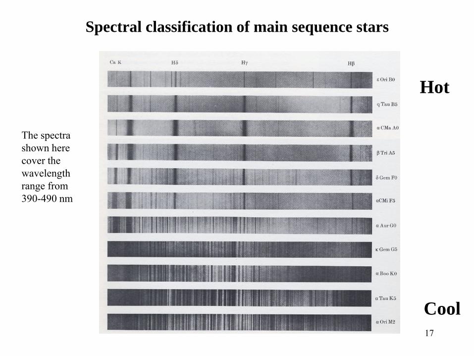
Spectral classification of main sequence stars

Hot

Cool

The spectra shown here cover the wavelength range from 390-490 nm

18

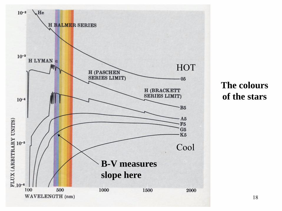
The colours of the stars

B-V measuresslope here

HOT

Cool

19

How do we measure luminosity?

• Absolute magnitude is a measure of luminosity and can be estimated from a star’s spectrum.

• Can use relative luminosities (i.e. apparent magnitudes) if all the stars plotted are at the same distance (i.e. in a star cluster).

20

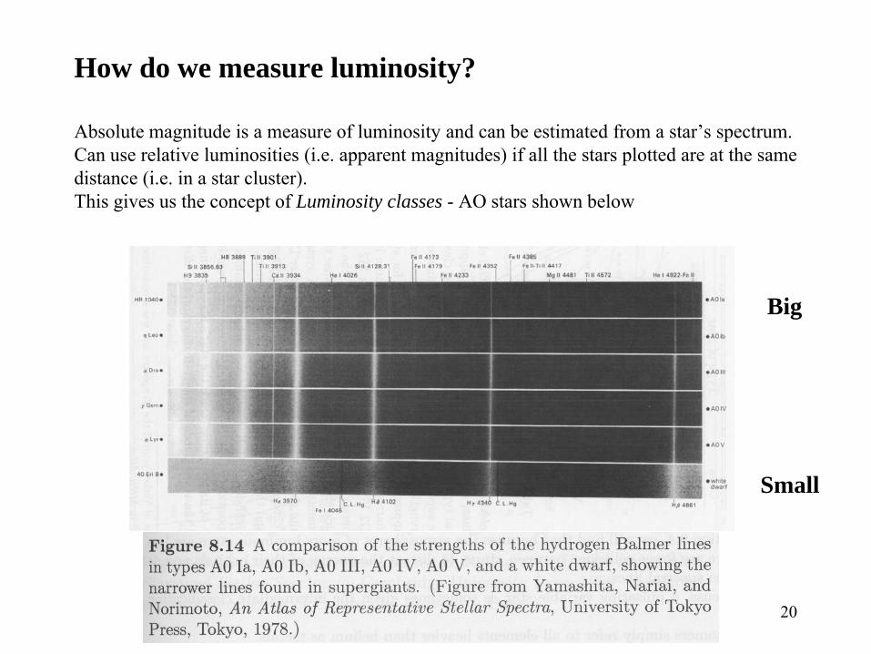
How do we measure luminosity?

Absolute magnitude is a measure of luminosity and can be estimated from a star’s spectrum.Can use relative luminosities (i.e. apparent magnitudes) if all the stars plotted are at the same distance (i.e. in a star cluster).This gives us the concept of Luminosity classes - AO stars shown below

Big

Small

21

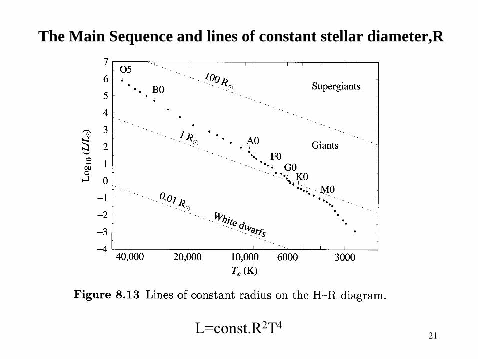
The Main Sequence and lines of constant stellar diameter,R

L=const.R2T4

22

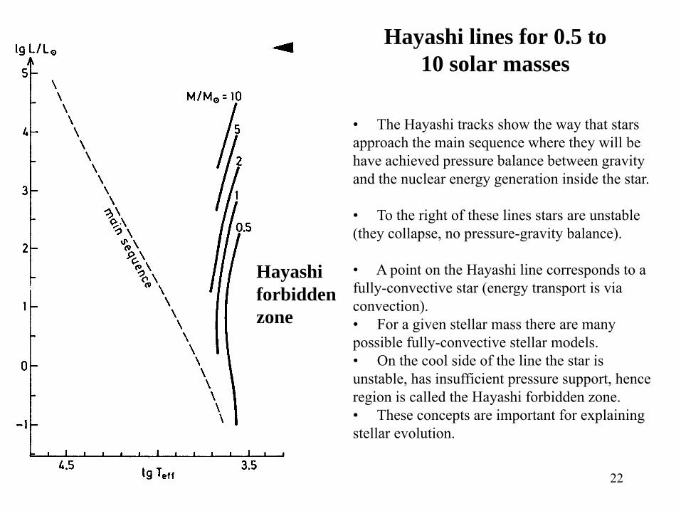
Hayashi lines for 0.5 to 10 solar masses

Hayashiforbiddenzone

• The Hayashi tracks show the way that stars approach the main sequence where they will be have achieved pressure balance between gravity and the nuclear energy generation inside the star.

• To the right of these lines stars are unstable (they collapse, no pressure-gravity balance).

• A point on the Hayashi line corresponds to a fully-convective star (energy transport is via convection).• For a given stellar mass there are many possible fully-convective stellar models.• On the cool side of the line the star is unstable, has insufficient pressure support, hence region is called the Hayashi forbidden zone.• These concepts are important for explaining stellar evolution.

23

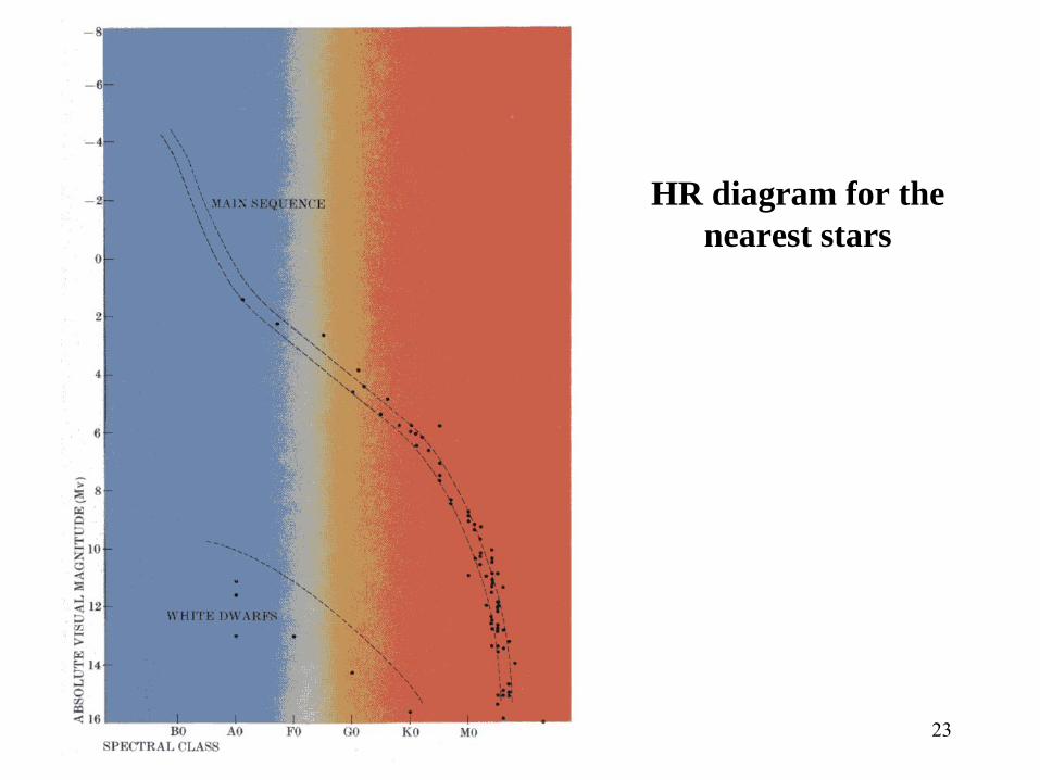
HR diagram for the nearest stars

24

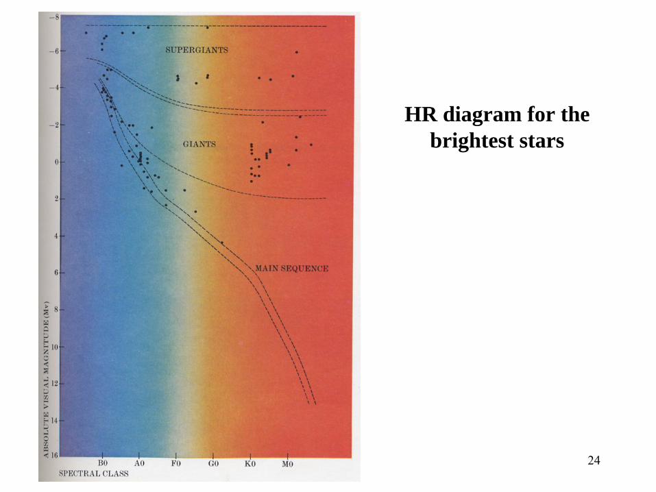
HR diagram for the brightest stars

25

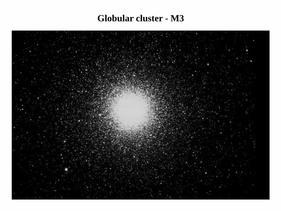
Globular cluster - M3

26

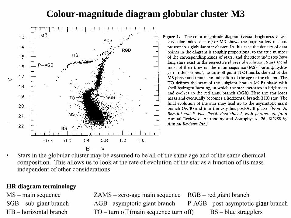
Colour-magnitude diagram globular cluster M3

BS

• Stars in the globular cluster may be assumed to be all of the same age and of the same chemical composition. This allows us to look at the rate of evolution of the star as a function of its mass independent of other considerations.

HR diagram terminologyMS – main sequence ZAMS – zero-age main sequence RGB – red giant branchSGB – sub-giant branch AGB - asymptotic giant branch P-AGB - post-asymptotic giant branchHB – horizontal branch TO – turn off (main sequence turn off) BS – blue stragglers

27

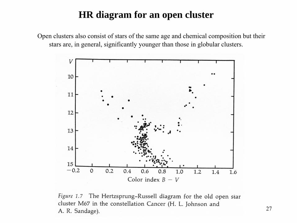
HR diagram for an open cluster

Open clusters also consist of stars of the same age and chemical composition but their stars are, in general, significantly younger than those in globular clusters.

28

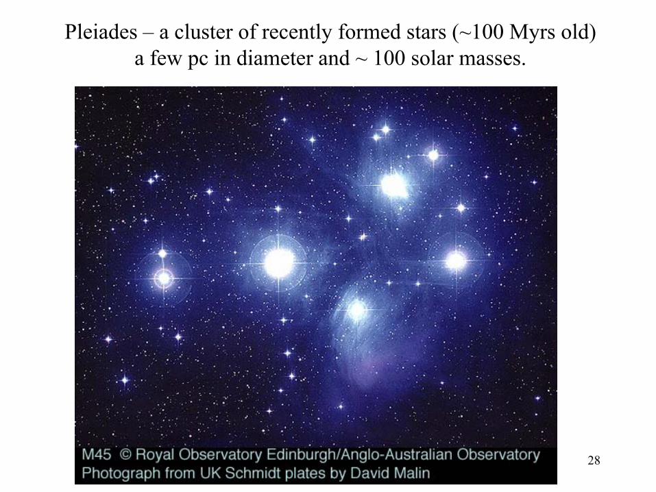
Pleiades – a cluster of recently formed stars (~100 Myrs old)a few pc in diameter and ~ 100 solar masses.

29

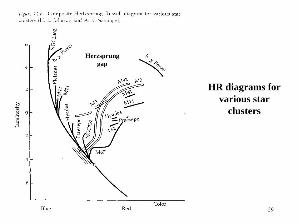
HR diagrams for various star

clusters

Herzsprunggap

30

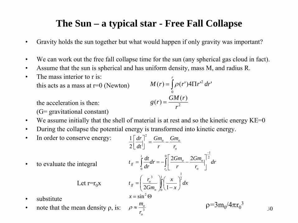
The Sun – a typical star - Free Fall Collapse

• Gravity holds the sun together but what would happen if only gravity was important?

• We can work out the free fall collapse time for the sun (any spherical gas cloud in fact).• Assume that the sun is spherical and has uniform density, mass M, and radius R.• The mass interior to r is:

this acts as a mass at r=0 (Newton)

the acceleration is then:(G= gravitational constant)

• We assume initially that the shell of material is at rest and so the kinetic energy KE=0• During the collapse the potential energy is transformed into kinetic energy.• In order to conserve energy:

• to evaluate the integral

• substitute• note that the mean density ρ, is:

2

0

2

)()(

''4)'()(

rrGMrg

drrrrMr

=

Π= ∫ ρ

Let r=r0x

ρ=3m0/4πr03

3

2

21

1

0

3

21

0

0

2

sin12

22

21

o

o

o

off

r o

oot

ff

o

oo

rm

x

dxx

xGmrt

drr

Gmr

Gmdrdrdtt

rGm

rGm

dtdr

o

≈

Θ=

⎟⎠⎞

⎜⎝⎛−⎟⎟

⎠

⎞⎜⎜⎝

⎛=

⎥⎦

⎤⎢⎣

⎡−−==

−=⎥⎦⎤

⎢⎣⎡

∫

∫∫−

ρ

31

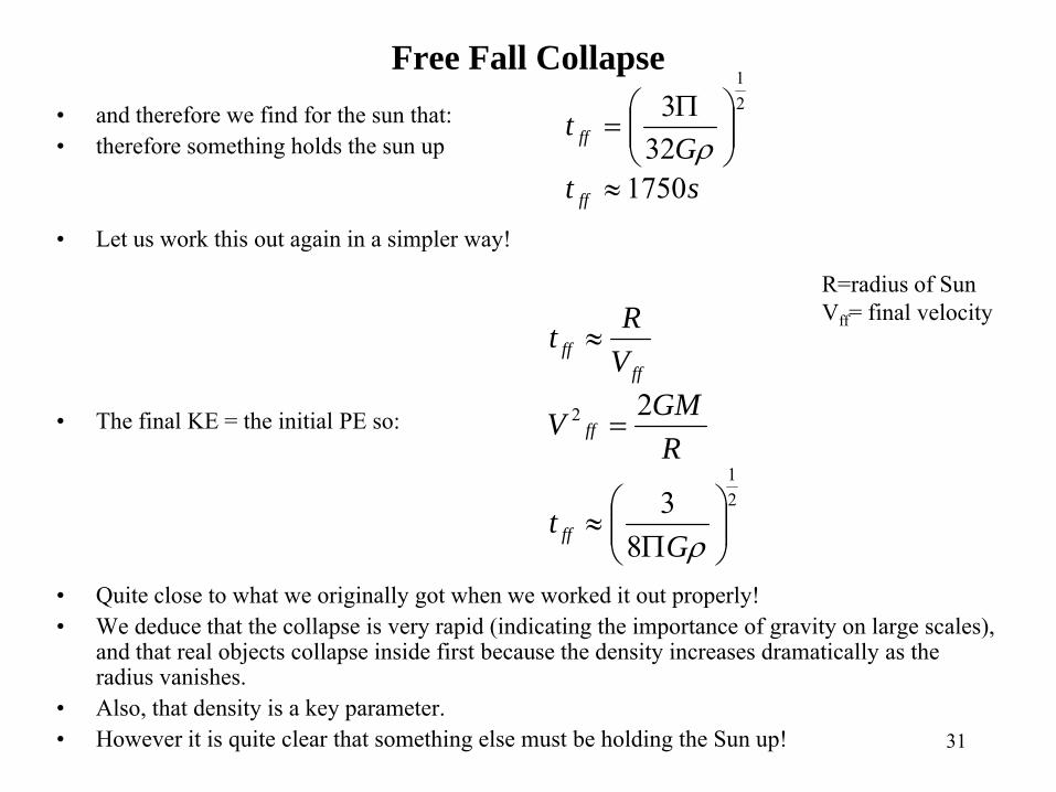
Free Fall Collapse• and therefore we find for the sun that:• therefore something holds the sun up

• Let us work this out again in a simpler way!

• The final KE = the initial PE so:

• Quite close to what we originally got when we worked it out properly!• We deduce that the collapse is very rapid (indicating the importance of gravity on large scales),

and that real objects collapse inside first because the density increases dramatically as the radius vanishes.

• Also, that density is a key parameter.• However it is quite clear that something else must be holding the Sun up!

stG

t

ff

ff

175032

3 21

≈

⎟⎟⎠

⎞⎜⎜⎝

⎛ Π=

ρ

21

2

83

2

⎟⎟⎠

⎞⎜⎜⎝

⎛Π

≈

=

≈

ρGt

RGMV

VRt

ff

ff

ffff

R=radius of SunVff= final velocity

32

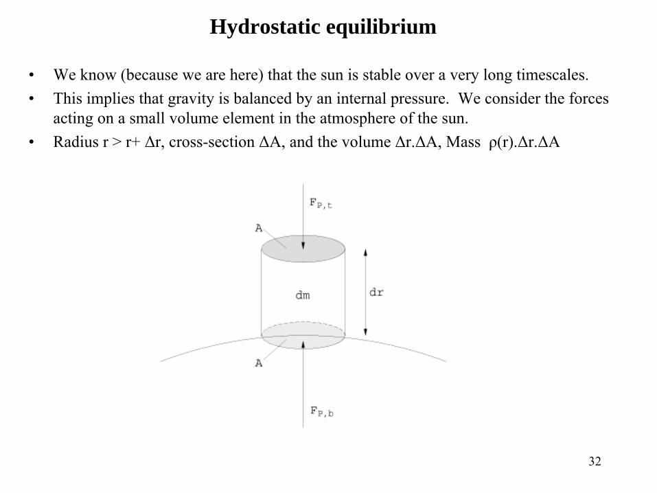
Hydrostatic equilibrium

• We know (because we are here) that the sun is stable over a very long timescales.• This implies that gravity is balanced by an internal pressure. We consider the forces

acting on a small volume element in the atmosphere of the sun.• Radius r > r+ Δr, cross-section ΔA, and the volume Δr.ΔA, Mass ρ(r).Δr.ΔA

33

Hydrostatic equilibrium

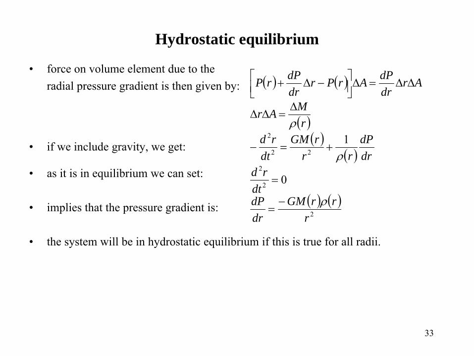
• force on volume element due to the radial pressure gradient is then given by:

• if we include gravity, we get:

• as it is in equilibrium we can set:

• implies that the pressure gradient is:

• the system will be in hydrostatic equilibrium if this is true for all radii.

( ) ( )

( )( )

( )

( ) ( )2

2

2

22

2

0

1

rrrGM

drdPdt

rddrdP

rrrGM

dtrd

rMAr

ArdrdPArPr

drdPrP

ρ

ρ

ρ

−=

=

+=−

Δ=ΔΔ

ΔΔ=Δ⎥⎦⎤

⎢⎣⎡ −Δ+

34

Kelvin-Helmholtz Timescale

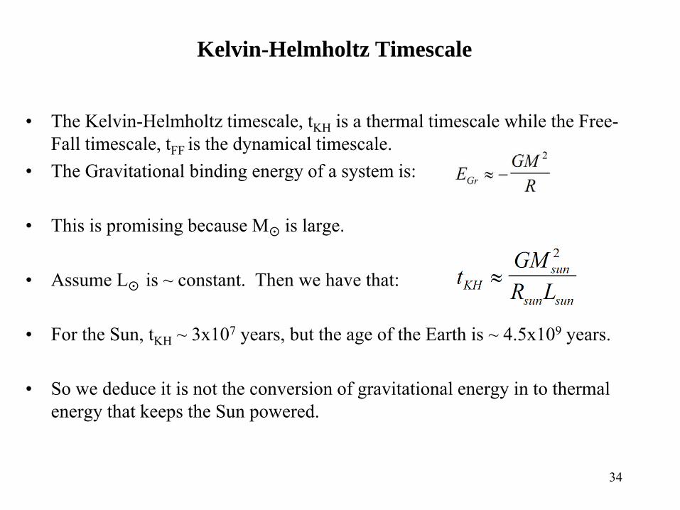
• The Kelvin-Helmholtz timescale, tKH is a thermal timescale while the Free-Fall timescale, tFF is the dynamical timescale.

• The Gravitational binding energy of a system is:

• This is promising because M is large.

• Assume L is ~ constant. Then we have that:

• For the Sun, tKH ~ 3x107 years, but the age of the Earth is ~ 4.5x109 years.

• So we deduce it is not the conversion of gravitational energy in to thermal energy that keeps the Sun powered.

35

The Virial Theorem

• For a self-gravitating system of particles which is in equilibrium it can be shown that

2KE = -PE

• This is the virial theorem.

• KE is the kinetic energy of the particles and PE is the gravitational potential energy of the particles.

• “In equilibrium” means the system is neither expanding or collapsing.• The particles could be atomic particles (system is a star) or stars (system is a star

cluster or galaxy) or galaxies (system is a cluster of galaxies).

36

Temperature and Pressure in the Sun

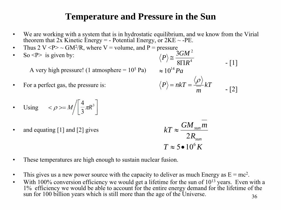
• We are working with a system that is in hydrostatic equilibrium, and we know from the Virial theorem that 2x Kinetic Energy = - Potential Energy, or 2KE ~ -PE.

• Thus 2 V <P> ~ GM2/R, where V = volume, and P = pressure• So <P> is given by:

A very high pressure! (1 atmosphere = 105 Pa)

• For a perfect gas, the pressure is:

• Using

• and equating [1] and [2] gives

• These temperatures are high enough to sustain nuclear fusion.

• This gives us a new power source with the capacity to deliver as much Energy as E = mc2. • With 100% conversion efficiency we would get a lifetime for the sun of 1013 years. Even with a

1% efficiency we would be able to account for the entire energy demand for the lifetime of the sun for 100 billion years which is still more than the age of the Universe.

kTm

nkTP

PaR

GMP

ρ==

≈Π

≅14

4

2

1083

- [1]

- [2]

KTR

mGMkTsun

sun

61052

•≈

≈

37

What supplies the energy for the Sun and the stars?

• Sun is ~4.5 billion years old.

• If its total gravitational energy is used up at its present luminosity it will last for ~30 million years.

• If the Sun’s mass was made of dynamite the available energy would only last 10,000 years.

• Virial theorem tells us that as the Sun contracts gravitational energy is converted into thermal and it gets hotter – so energy source can’t be the thermal energy. (Note: this implies a self gravitating object like a star has negative specific heat).

• If the sun is made entirely of H and all this is turned to He by nuclear burning then lifetime at present luminosity is 100 billion years – must be nuclear.

38

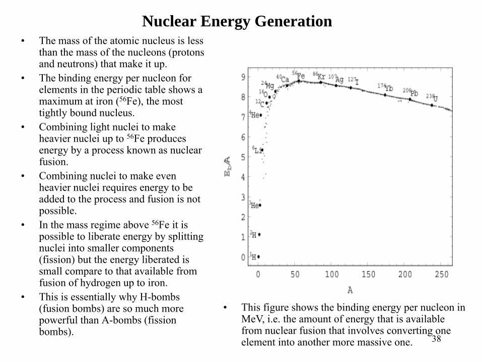
Nuclear Energy Generation• The mass of the atomic nucleus is less

than the mass of the nucleons (protons and neutrons) that make it up.

• The binding energy per nucleon for elements in the periodic table shows a maximum at iron (56Fe), the most tightly bound nucleus.

• Combining light nuclei to make heavier nuclei up to 56Fe produces energy by a process known as nuclear fusion.

• Combining nuclei to make even heavier nuclei requires energy to be added to the process and fusion is not possible.

• In the mass regime above 56Fe it is possible to liberate energy by splitting nuclei into smaller components (fission) but the energy liberated is small compare to that available from fusion of hydrogen up to iron.

• This is essentially why H-bombs (fusion bombs) are so much more powerful than A-bombs (fission bombs).

• This figure shows the binding energy per nucleon in MeV, i.e. the amount of energy that is available from nuclear fusion that involves converting one element into another more massive one.

39

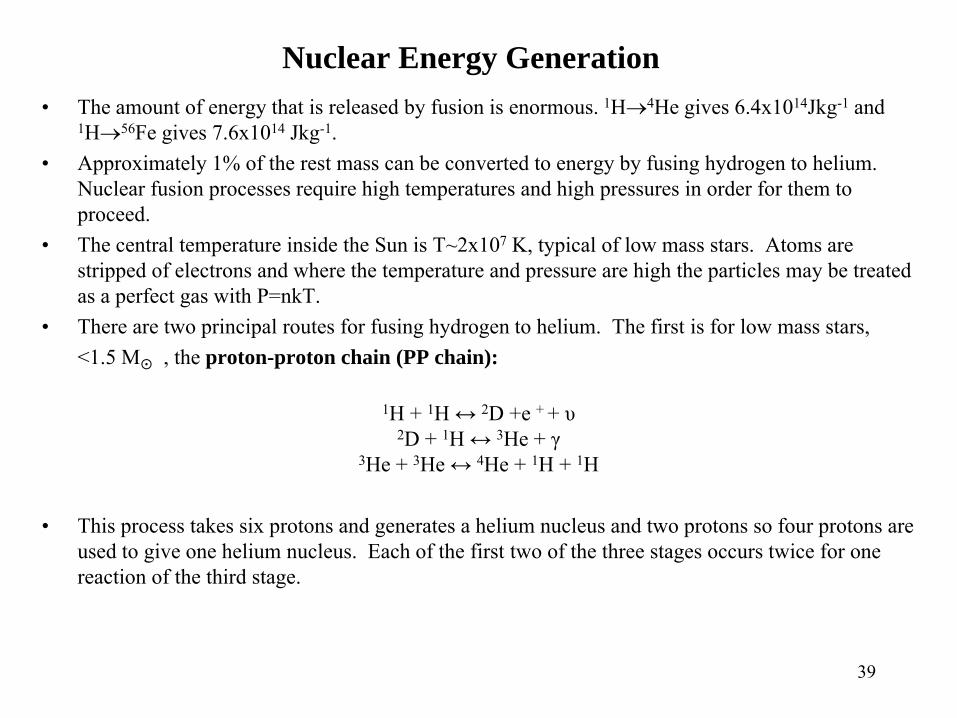
Nuclear Energy Generation• The amount of energy that is released by fusion is enormous. 1H→4He gives 6.4x1014Jkg-1 and

1H→56Fe gives 7.6x1014 Jkg-1. • Approximately 1% of the rest mass can be converted to energy by fusing hydrogen to helium.

Nuclear fusion processes require high temperatures and high pressures in order for them to proceed.

• The central temperature inside the Sun is T~2x107 K, typical of low mass stars. Atoms are stripped of electrons and where the temperature and pressure are high the particles may be treated as a perfect gas with P=nkT.

• There are two principal routes for fusing hydrogen to helium. The first is for low mass stars,<1.5 M , the proton-proton chain (PP chain):

1H + 1H ↔ 2D +e + + υ2D + 1H ↔ 3He + γ

3He + 3He ↔ 4He + 1H + 1H

• This process takes six protons and generates a helium nucleus and two protons so four protons are used to give one helium nucleus. Each of the first two of the three stages occurs twice for one reaction of the third stage.

40

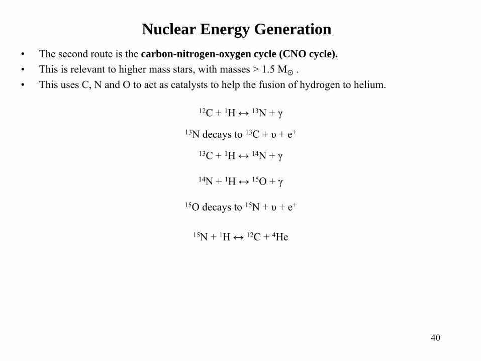
Nuclear Energy Generation• The second route is the carbon-nitrogen-oxygen cycle (CNO cycle). • This is relevant to higher mass stars, with masses > 1.5 M .• This uses C, N and O to act as catalysts to help the fusion of hydrogen to helium.

12C + 1H ↔ 13N + γ

13N decays to 13C + υ + e+

13C + 1H ↔ 14N + γ

14N + 1H ↔ 15O + γ

15O decays to 15N + υ + e+

15N + 1H ↔ 12C + 4He

41

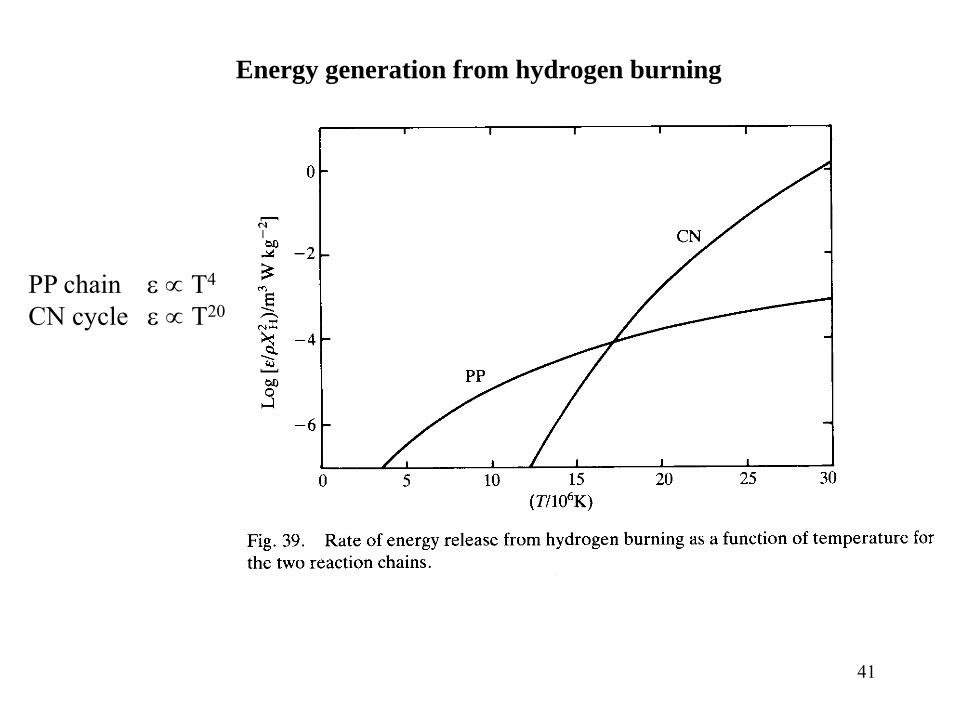
Energy generation from hydrogen burning

PP chain ε ∝ T4

CN cycle ε ∝ T20

42

Stellar Evolution

• Stars spend most of their life burning hydrogen into helium.• Hydrogen is the main constituent and it is the transformation of hydrogen into helium

which liberates most of the energy available by nucleosynthesis in stars.• The nuclear fusion processes are extremely sensitive to temperature.• The higher mass stars have very much higher central temperatures and therefore

much higher luminosities.• We find that L~ M3 approximately for H-core-burning stars (i.e. stars on the main

sequence).• Provided stars are sufficiently massive (M>~8Msun) they will be hot enough such that

fusion of carbon, oxygen etc. all the way up to iron is possible.• Fusion of He takes place via the triple α process. This three-particle process is

necessary because it overcomes the the lack of stable nuclei with progressively increasing binding energy between helium and carbon.

• Here we have:4He + 4He ↔ 8Be + γ - 91.78 KeV8Be + 4He → 12C + γ + 7.367 MeV

43

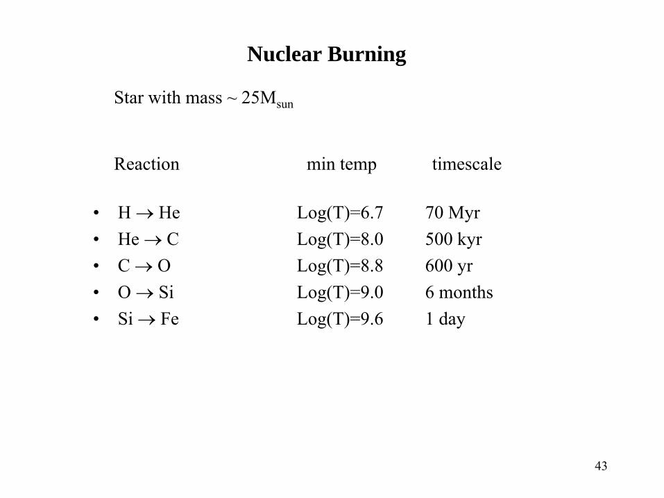
Nuclear Burning

• H → He Log(T)=6.7 70 Myr• He → C Log(T)=8.0 500 kyr• C → O Log(T)=8.8 600 yr• O → Si Log(T)=9.0 6 months• Si → Fe Log(T)=9.6 1 day

Star with mass ~ 25Msun

Reaction min temp timescale

44

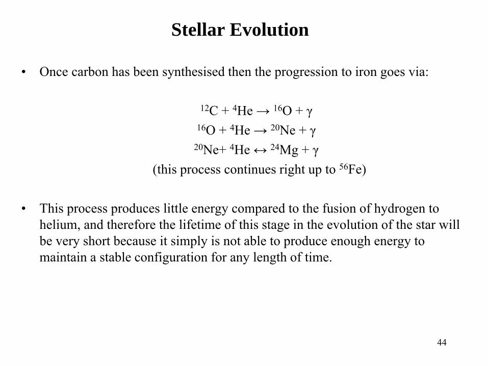
Stellar Evolution

• Once carbon has been synthesised then the progression to iron goes via:

12C + 4He → 16O + γ 16O + 4He → 20Ne + γ

20Ne+ 4He ↔ 24Mg + γ (this process continues right up to 56Fe)

• This process produces little energy compared to the fusion of hydrogen to helium, and therefore the lifetime of this stage in the evolution of the star will be very short because it simply is not able to produce enough energy to maintain a stable configuration for any length of time.

45

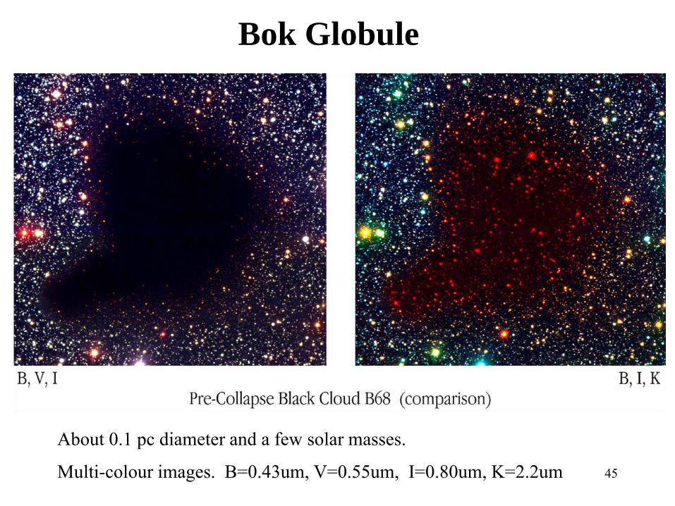
Bok Globule

About 0.1 pc diameter and a few solar masses.

Multi-colour images. B=0.43um, V=0.55um, I=0.80um, K=2.2um

46

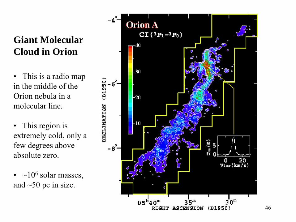
Giant Molecular Cloud in Orion

• This is a radio map in the middle of the Orion nebula in a molecular line.

• This region is extremely cold, only a few degrees above absolute zero.

• ~106 solar masses, and ~50 pc in size.

47

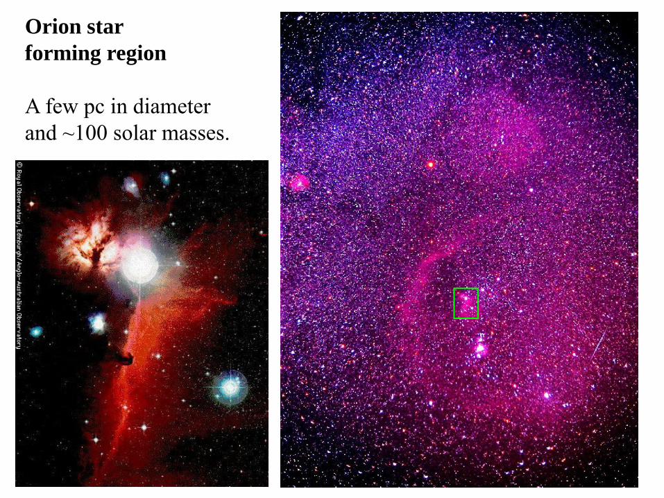
Orion starforming region

A few pc in diameter and ~100 solar masses.

48

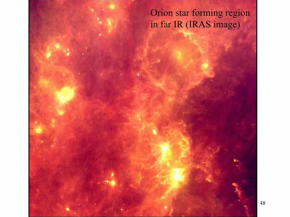
Orion star forming regionin far IR (IRAS image)

49

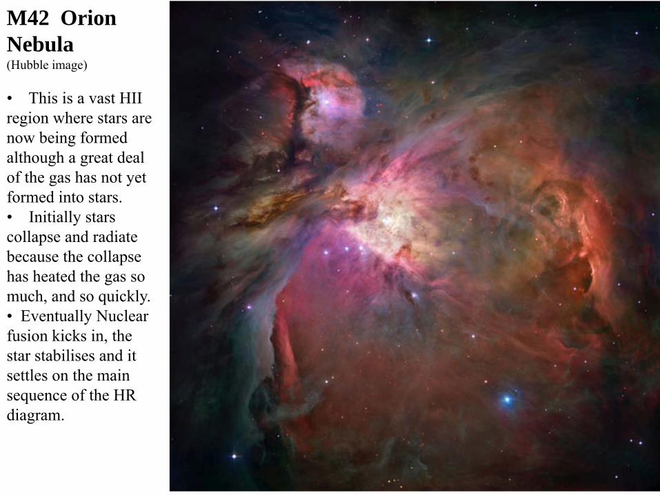
M42 Orion Nebula(Hubble image)

• This is a vast HII region where stars are now being formed although a great deal of the gas has not yet formed into stars.• Initially stars collapse and radiate because the collapse has heated the gas so much, and so quickly.• Eventually Nuclear fusion kicks in, the star stabilises and it settles on the main sequence of the HR diagram.

50

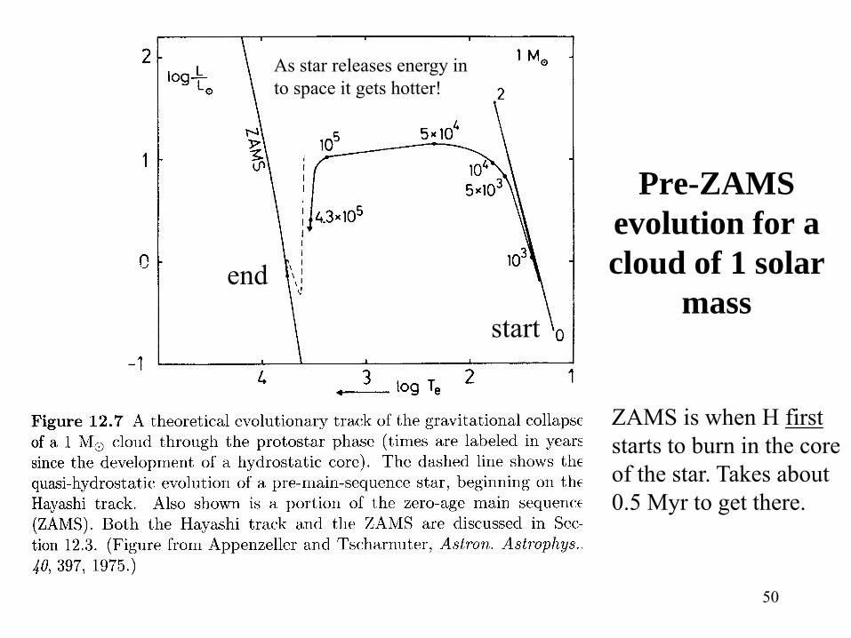
Pre-ZAMS evolution for a cloud of 1 solar

mass

ZAMS is when H firststarts to burn in the core of the star. Takes about 0.5 Myr to get there.

As star releases energy in to space it gets hotter!

start

end

51

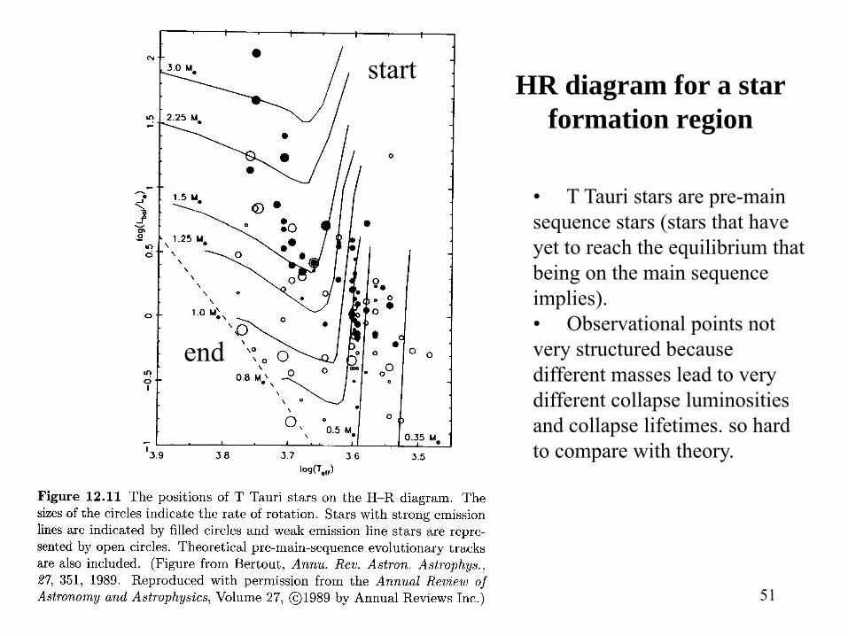
HR diagram for a star formation region

start

end

• T Tauri stars are pre-main sequence stars (stars that have yet to reach the equilibrium that being on the main sequence implies).• Observational points not very structured because different masses lead to very different collapse luminosities and collapse lifetimes. so hard to compare with theory.

52

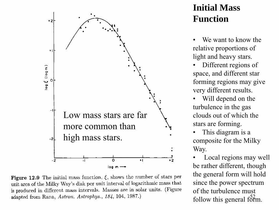
Low mass stars are far more common than high mass stars.

Initial Mass Function

• We want to know the relative proportions of light and heavy stars. • Different regions of space, and different star forming regions may give very different results.• Will depend on the turbulence in the gas clouds out of which the stars are forming.• This diagram is a composite for the Milky Way.• Local regions may well be rather different, though the general form will hold since the power spectrum of the turbulence must follow this general form.

53

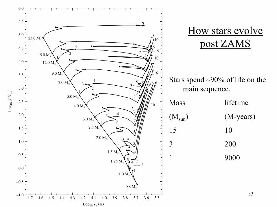
How stars evolve post ZAMS

Stars spend ~90% of life on the main sequence.

Mass lifetime

(Msun) (M-years)

15 10

3 200

1 9000

54

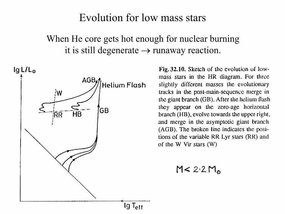
Evolution for low mass stars

When He core gets hot enough for nuclear burning it is still degenerate → runaway reaction.

55

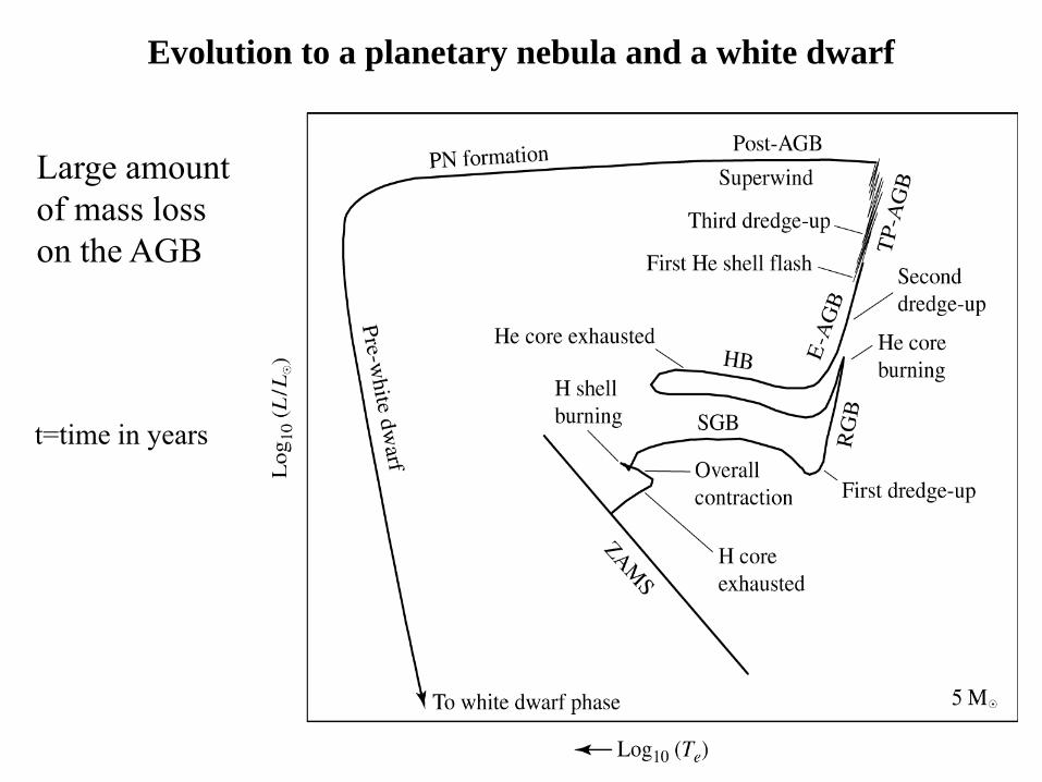
Evolution to a planetary nebula and a white dwarf

t=time in years

Large amount of mass loss on the AGB

56

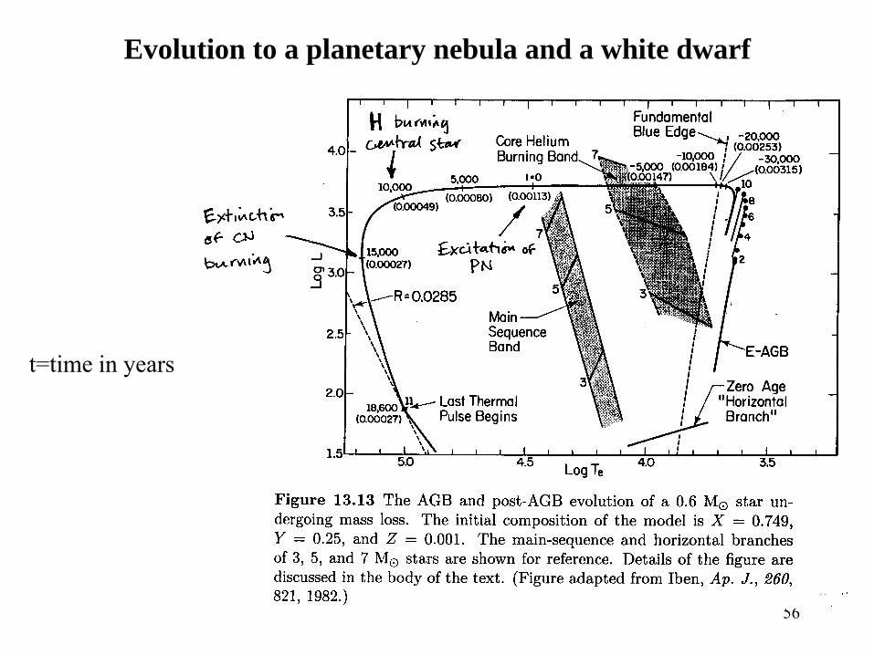
Evolution to a planetary nebula and a white dwarf

t=time in years

57

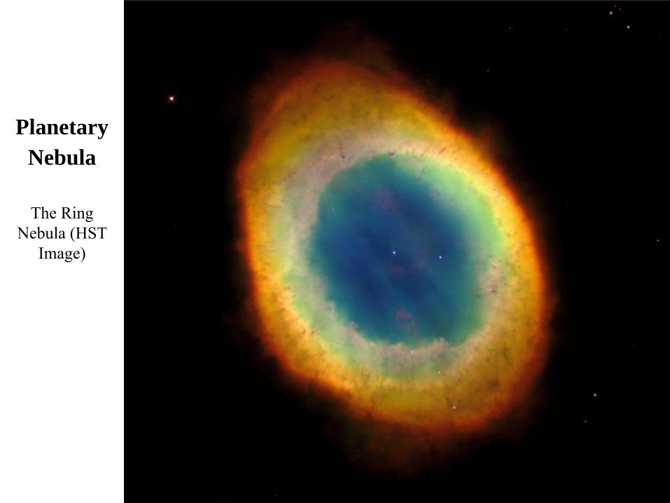
Planetary Nebula

The Ring Nebula (HST

Image)

58

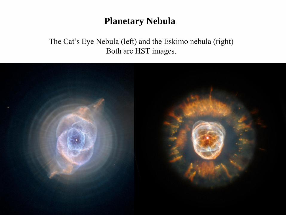
Planetary Nebula

The Cat’s Eye Nebula (left) and the Eskimo nebula (right)Both are HST images.

59

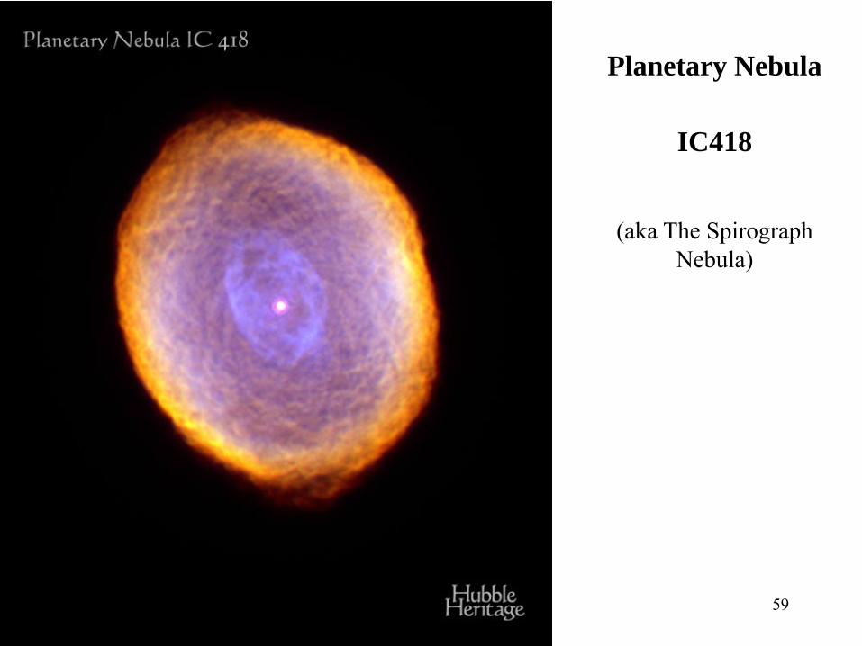
Planetary Nebula

IC418

(aka The Spirograph Nebula)

60

Supernovae

• Once star has an Fe core it cannot burn nuclear fuel at the core and therefore cannot provide enough pressure support.

• Star collapses catastrophically.• Core eventually is supported by a degenerate neutron gas• Infalling outer envelope bounces → enormous super nova explosion.

61

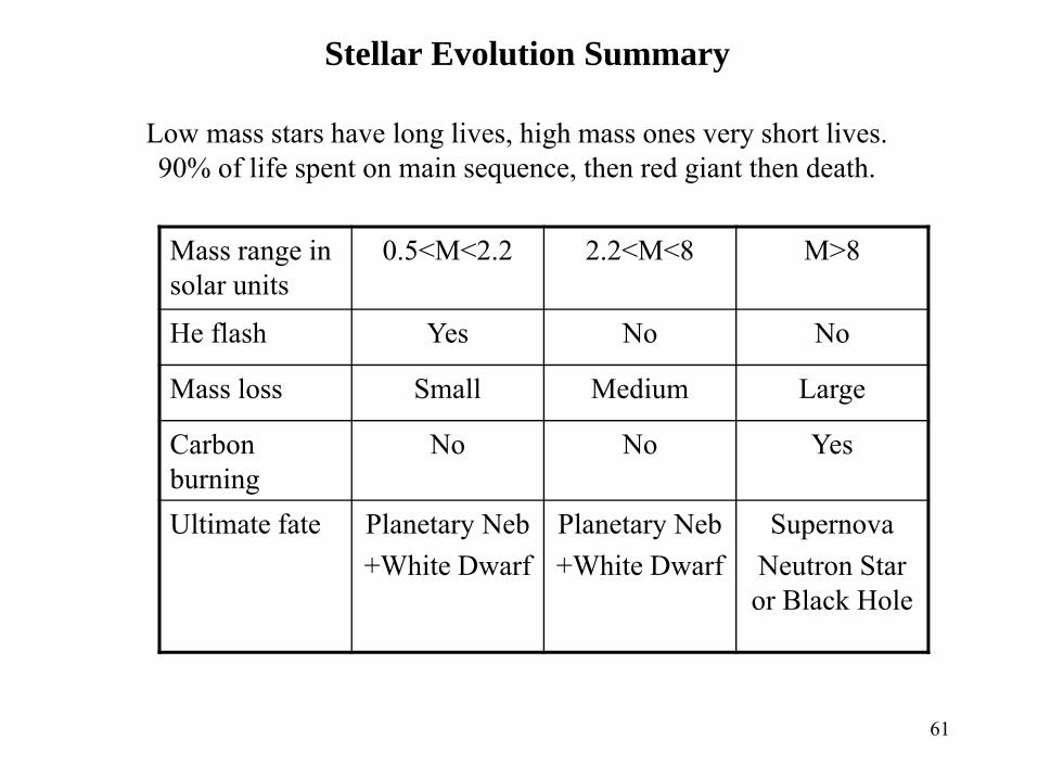
Stellar Evolution Summary

Mass range in solar units

0.5<M<2.2 2.2<M<8 M>8

He flash Yes No No

Mass loss Small Medium Large

Carbon burning

No No Yes

Ultimate fate Planetary Neb+White Dwarf

Planetary Neb+White Dwarf

SupernovaNeutron Star or Black Hole

Low mass stars have long lives, high mass ones very short lives.90% of life spent on main sequence, then red giant then death.

62

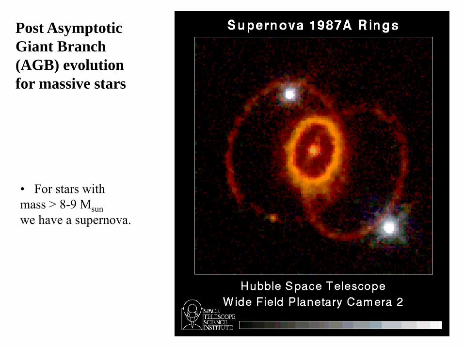
• For stars with mass > 8-9 Msunwe have a supernova.

Post Asymptotic Giant Branch (AGB) evolution for massive stars

63

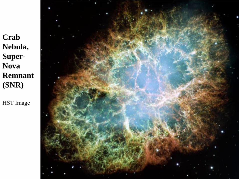
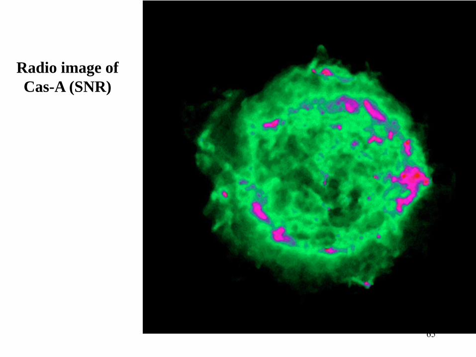
CrabNebula,Super-NovaRemnant(SNR)

HST Image

64

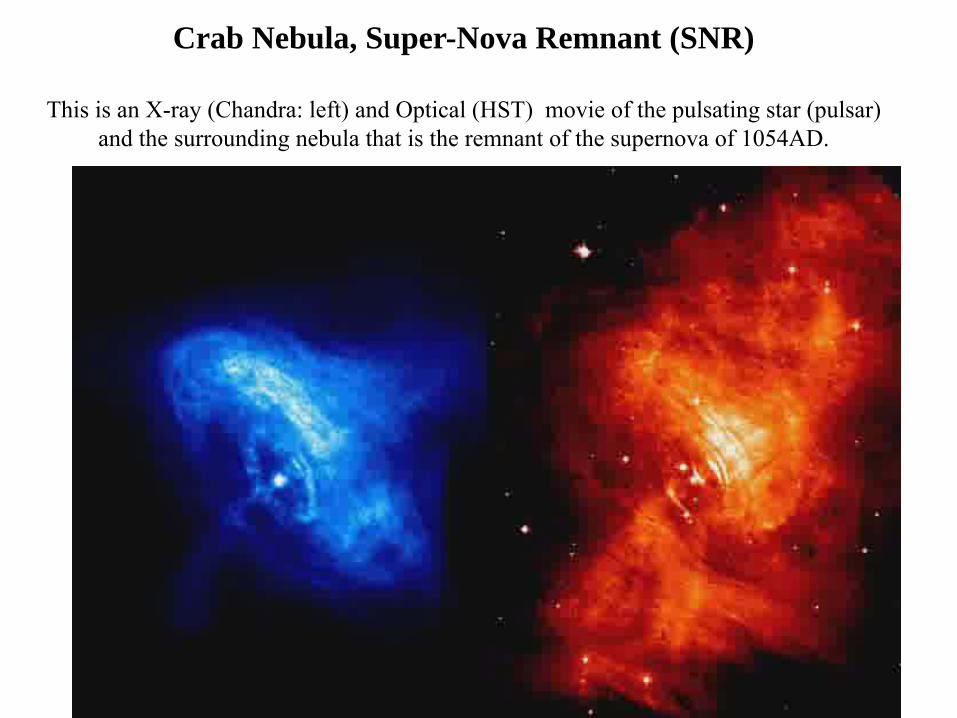
Crab Nebula, Super-Nova Remnant (SNR)

This is an X-ray (Chandra: left) and Optical (HST) movie of the pulsating star (pulsar) and the surrounding nebula that is the remnant of the supernova of 1054AD.

65

Radio image of Cas-A (SNR)

66

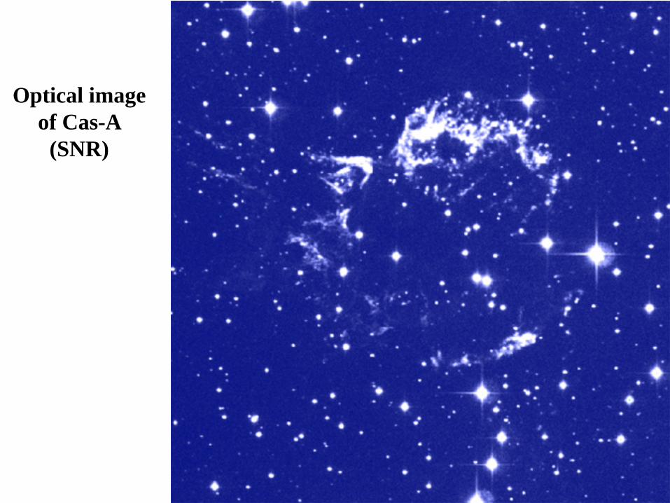
Optical image of Cas-A

(SNR)

67

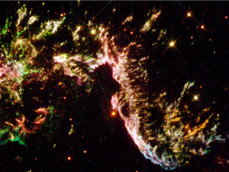
Optical image of part of Cas-A (SNR)

HST Image

68

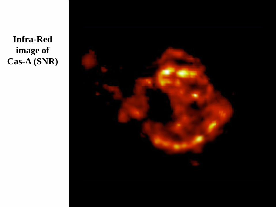
Infra-Red image of

Cas-A (SNR)

69

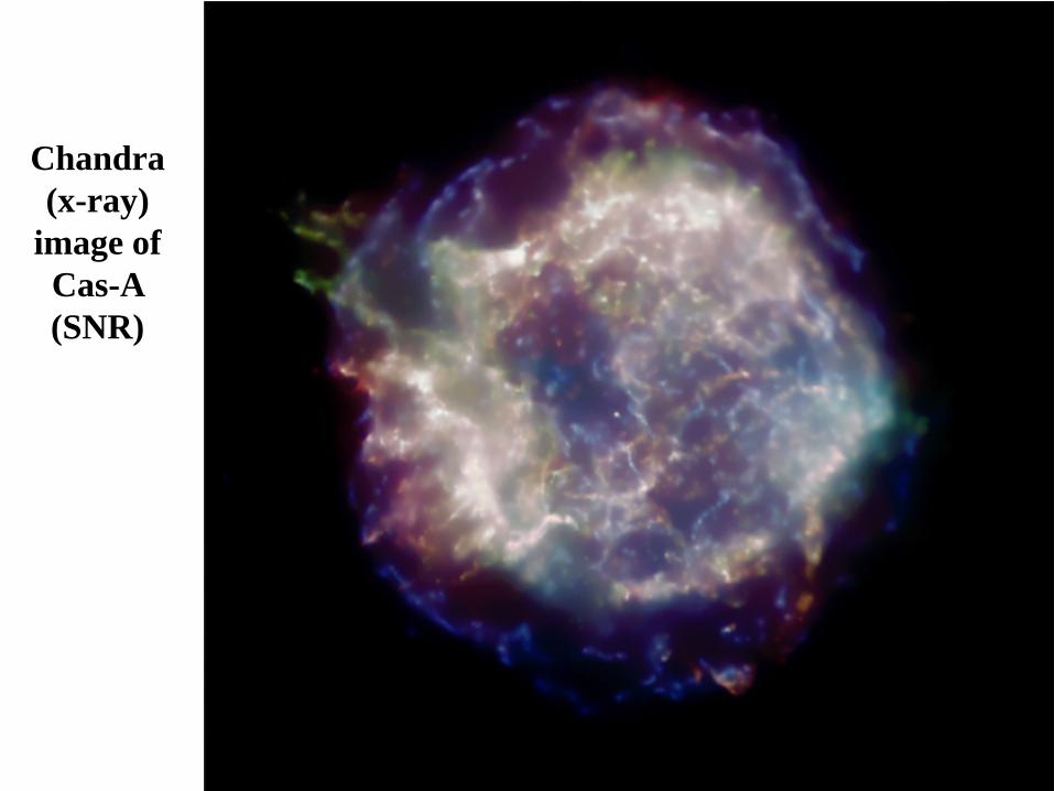
Chandra (x-ray)

image of Cas-A (SNR)

70

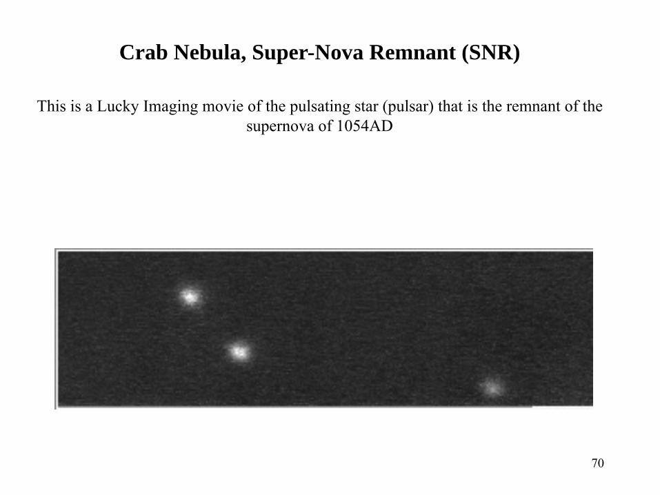
Crab Nebula, Super-Nova Remnant (SNR)

This is a Lucky Imaging movie of the pulsating star (pulsar) that is the remnant of the supernova of 1054AD

71

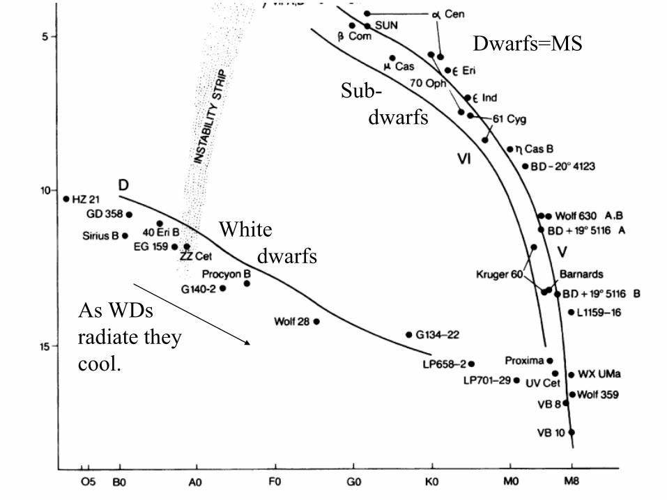
Whitedwarfs

Sub-dwarfs

Dwarfs=MS

As WDsradiate theycool.

72

Binary stars

• Most stars are in binary systems.• Evolution in a binary system can be radically changed by mass

exchange, especially when the stars are close together.• We will come back to this later in the course.

73

Orbits-1: Kepler’s Laws

• Kepler’s 1st law: A planet orbits the Sun in an ellipse with the Sun at one focus of the ellipse

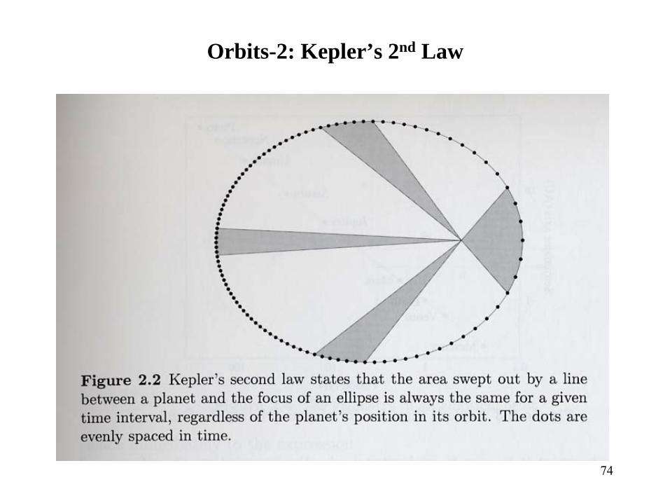
• Kepler’s 2nd law: A line connecting a planet to the Sun sweeps out equal areas in equal time intervals

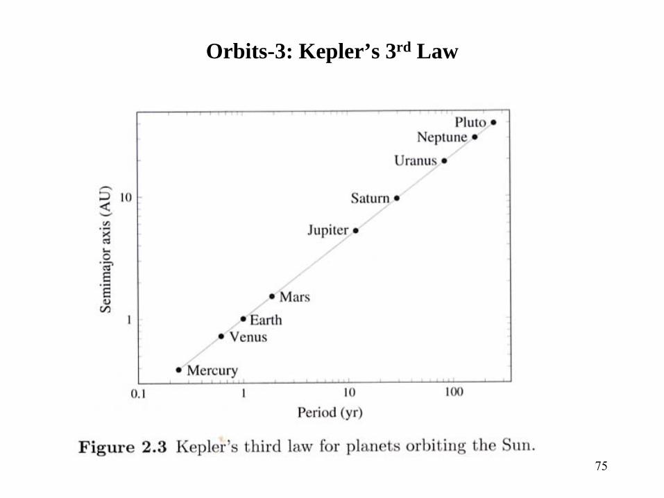
• Kepler’s 3rd law: [Period(years)]2=[semi-major axis(AU)]3 (specific to orbits around the Sun)

74

Orbits-2: Kepler’s 2nd Law

75

Orbits-3: Kepler’s 3rd Law

76

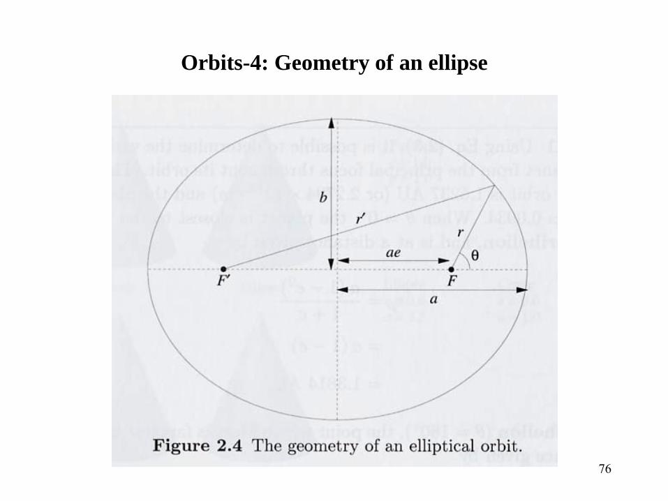
Orbits-4: Geometry of an ellipse

77

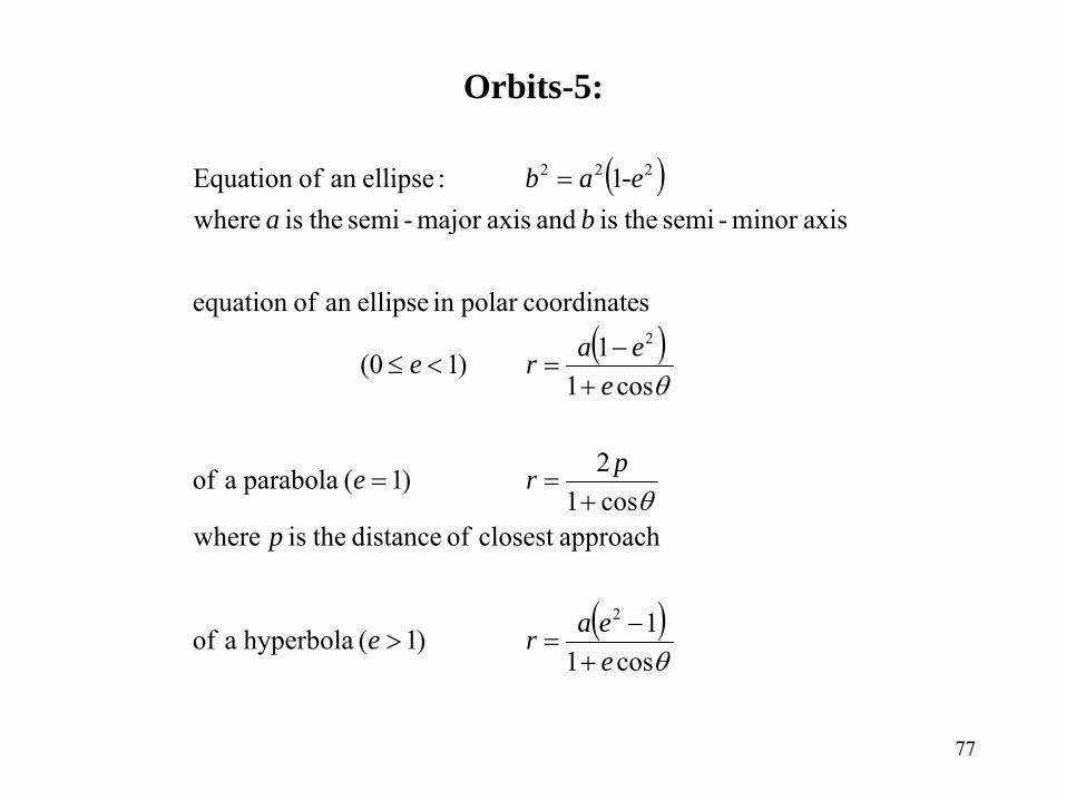
Orbits-5:

( )

( )

( )θ

θ

θ

cos11)1( hyperbola a of

approachclosest of distance theis wherecos12)1( parabola a of

cos11)1(0

scoordinatepolar in ellipsean ofequation

axisminor -semi theis and axismajor -semi theis where1 :ellipsean ofEquation

2

2

222

eeare

p

pre

eeare

ba-eab

+−

=>

+==

+−

=<≤

=

78

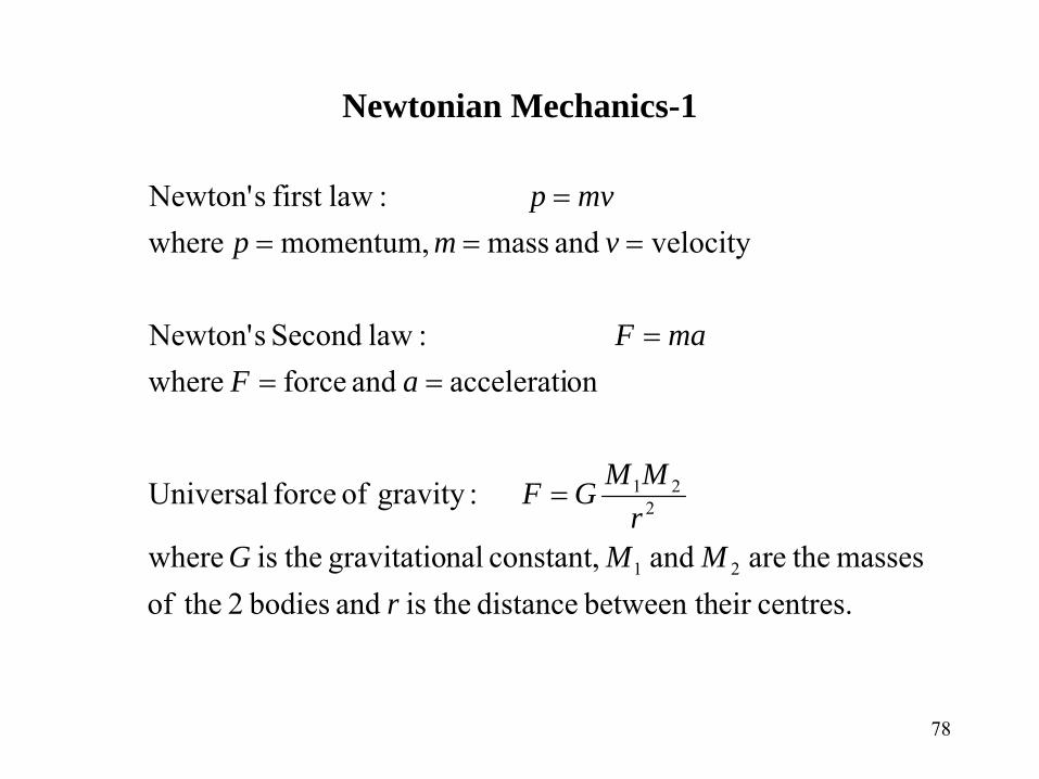
Newtonian Mechanics-1

centres.eir between th distance theis and bodies 2 theofmasses theare and constant, nalgravitatio theis where

:gravity of force Universal

onaccelerati and force where :law Second sNewton'

velocity and mass momentum, where :lawfirst sNewton'

21

221

rMMG

rMMGF

aFmaF

vmpmvp

=

===

====

79

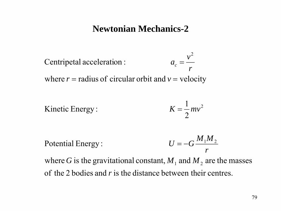
Newtonian Mechanics-2

centres.eir between th distancetheisandbodies 2 theofmasses theare and constant, nalgravitatio theis where

:Energy Potential

21 :Energy Kinetic

velocity andorbit circular of radius where

:onaccelerati lCentripeta

21

21

2

2

rMMG

rMMGU

mvK

vrrvac

−=

=

==

=

80

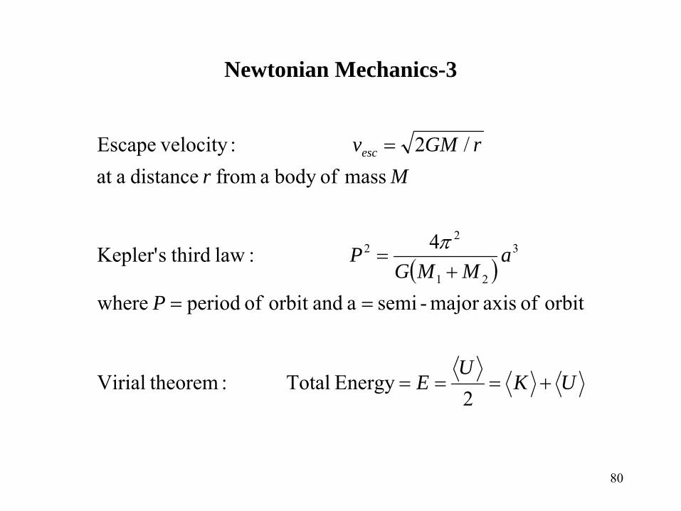
Newtonian Mechanics-3

( )

UKU

E

P

aMMG

P

MrrGMvesc

+===

==+

=

=

2Energy Total : theoremVirial

orbit of axismajor -semia andorbit of period where

4 :law thirdsKepler'

mass ofbody a from distance aat /2 : velocityEscape

3

21

22 π

81

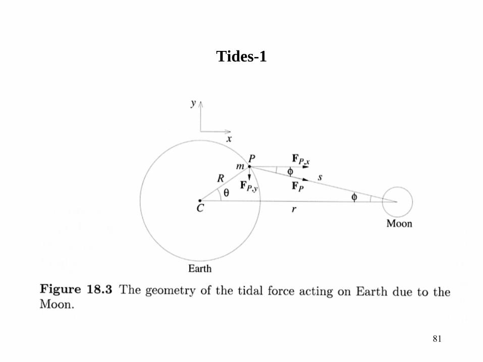
Tides-1

82

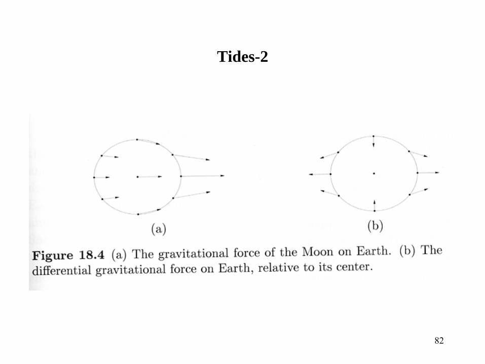
Tides-2

83

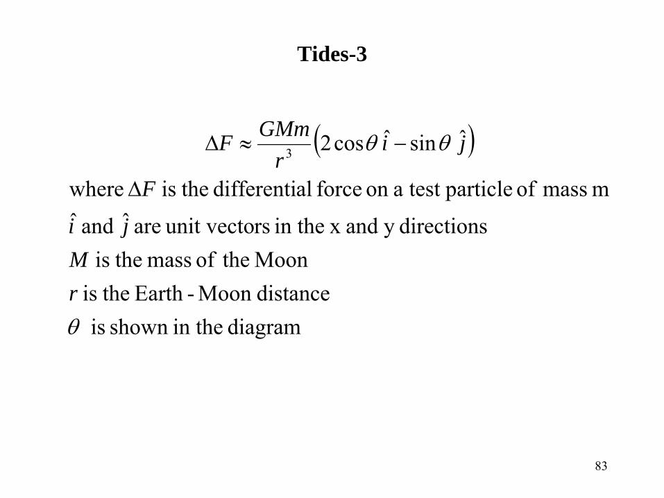
Tides-3

( )

diagram in theshown is distanceMoon -Earth theis Moon theof mass theis

directionsy and x in the rsunit vecto are ˆ and ˆm mass of particle test aon force aldifferenti theis where

ˆsinˆcos23

θ

θθ

rM

ji

F

jir

GMmF

Δ

−≈Δ

84

Tides-4

• Symmetry gives 2 tides every 24h 54m• Tidal friction causes the Earth to spin down, the day is getting longer

by 0.0016 sec/century• Moon has stopped spinning with respect to Earth• Moon is drifting away at 3 to 4 cm/year (conservation of angular

momentum)• Spring tide at new/full moon, Sun and Moon work together• Neap tides at 1st and 3rd quarter

85

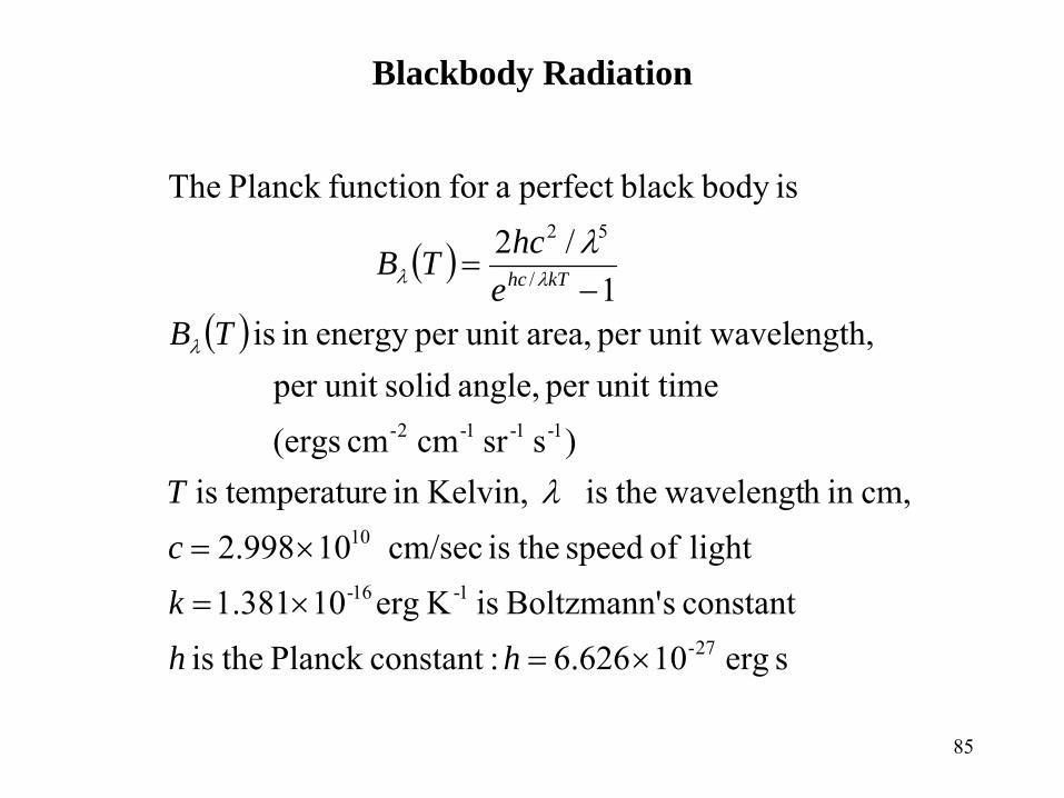
Blackbody Radiation

( )

( )

s erg 106.626 :constantPlanck theis constant sBoltzmann' is K erg101.381 light of speed theis cm/sec 102.998

cm,in h wavelengt theis Kelvin,in re temperatuis )s sr cm cm (ergs

unit timeper angle, solidunit per ength,unit wavelper area,unit per energy in is

1/2

isbody black perfect afor function Planck The

27-

1-16-

10

1-1-1-2-

/

52

×=

×=

×=

−=

hhkcT

TBe

hcTB kThc

λ

λ

λ

λλ

86

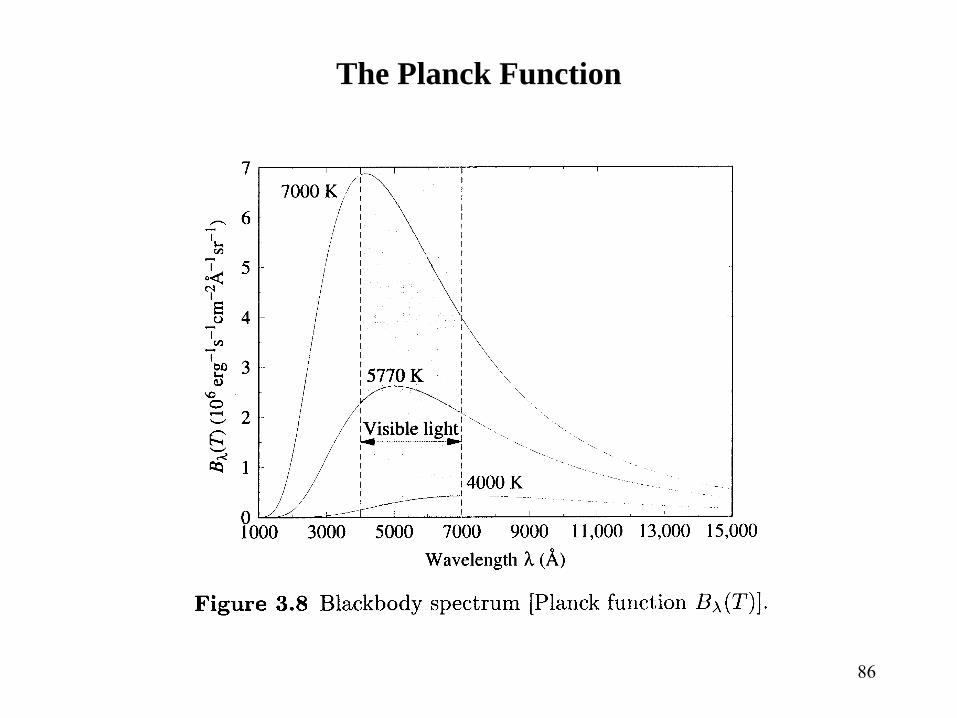
The Planck Function

87

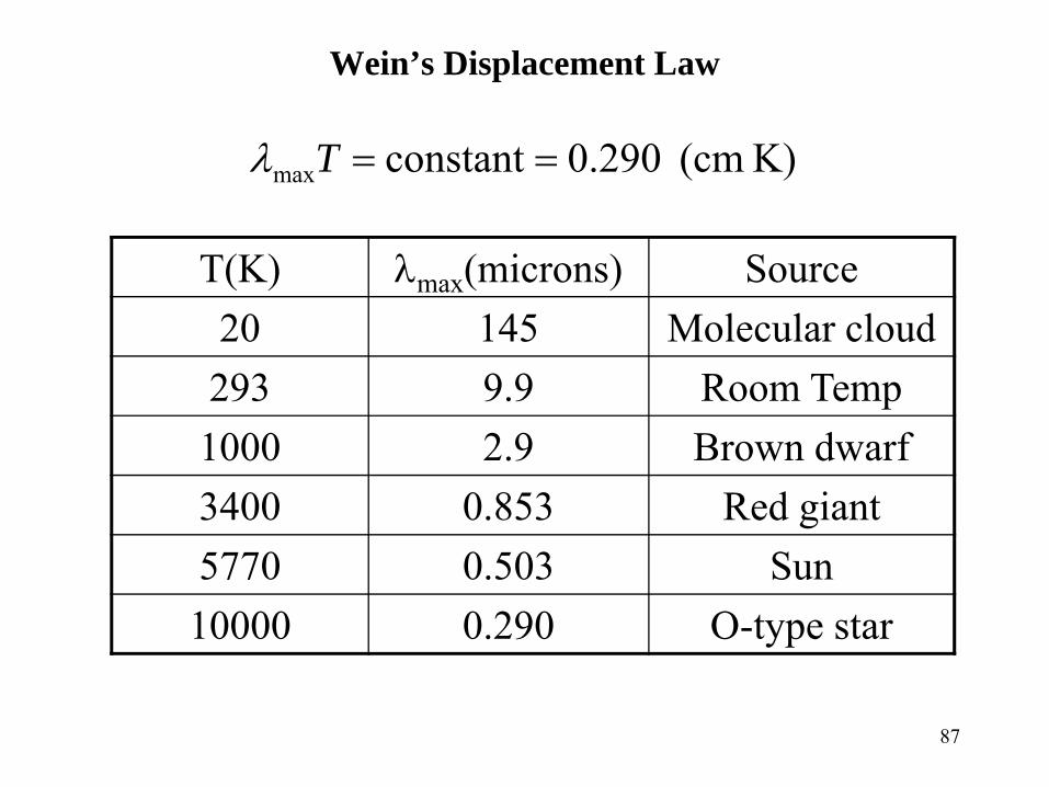
Wein’s Displacement Law

T(K) λmax(microns) Source20 145 Molecular cloud

293 9.9 Room Temp1000 2.9 Brown dwarf3400 0.853 Red giant5770 0.503 Sun10000 0.290 O-type star

K) (cm 290.0constantmax ==Tλ

88

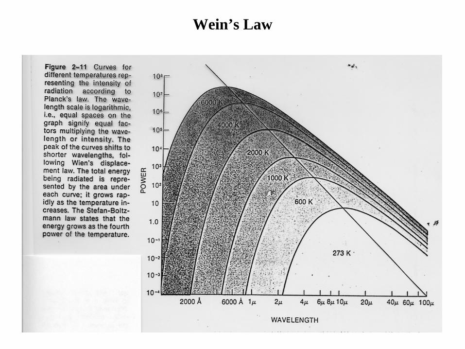
Wein’s Law

89

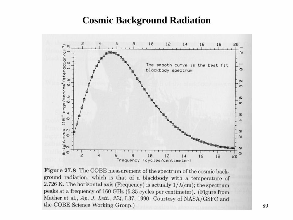
Cosmic Background Radiation

90

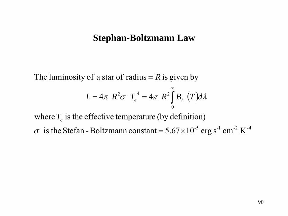
Stephan-Boltzmann Law

( )

4-2-1-5-

0

242

K cm s erg 105.67constant Boltzmann -Stefan theis

)definition(by re temperatueffective theis where

44

bygiven is radius ofstar a of luminosity The

×=

==

=

∫∞

σ

λπσπ λ

e

e

T

dTBRTRL

R

91

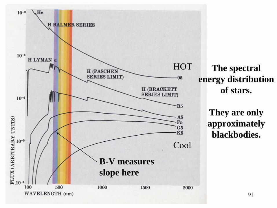
B-V measuresslope here

HOT

Cool

The spectral energy distribution

of stars.

They are only approximately blackbodies.

92

Electromagnetic Radiation

• When a charged particle is accelerated (loses energy) it gives rise to electromagnetic radiation.

• When electro-magnetic radiation is absorbed it accelerates a charged particle.

93

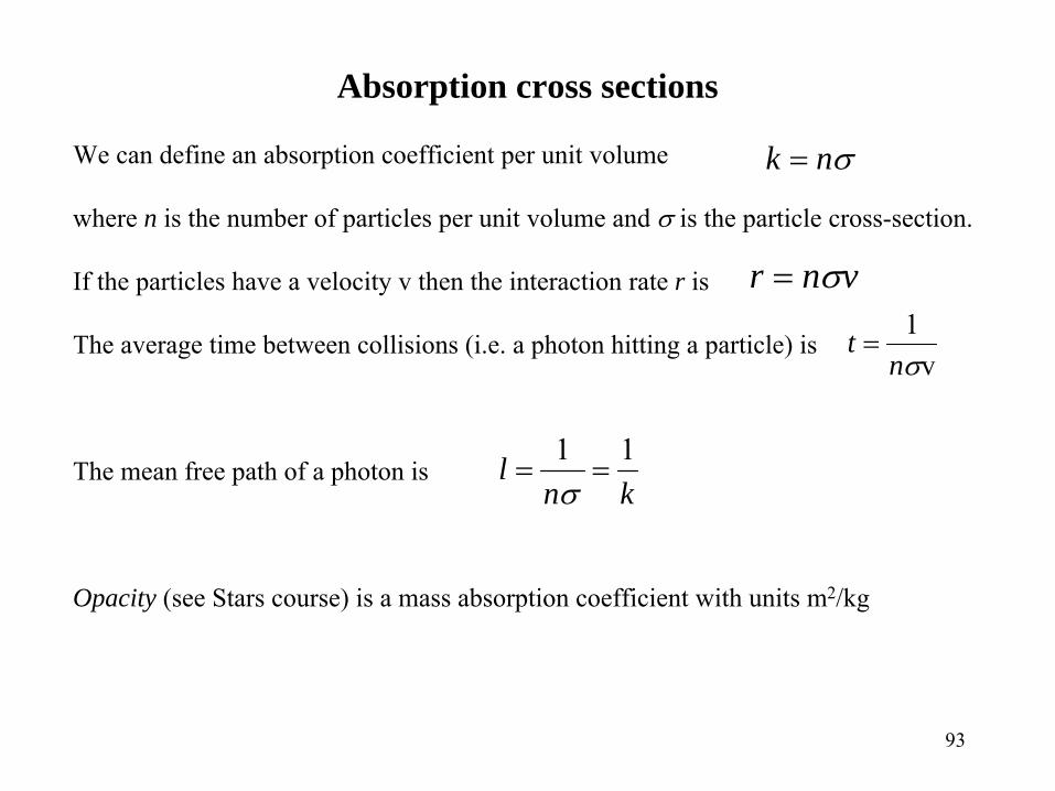
Absorption cross sections

We can define an absorption coefficient per unit volume

where n is the number of particles per unit volume and σ is the particle cross-section.

If the particles have a velocity v then the interaction rate r is

The average time between collisions (i.e. a photon hitting a particle) is

The mean free path of a photon is

Opacity (see Stars course) is a mass absorption coefficient with units m2/kg

v1σn

t =

σnk =

vnr σ=

knl 11

==σ

94

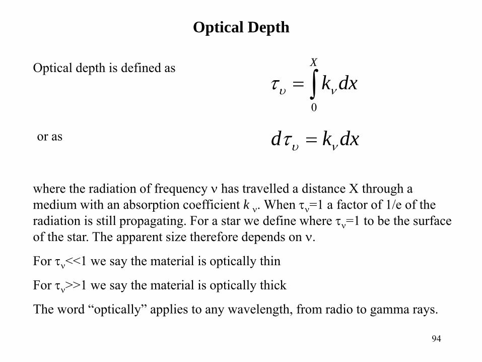
Optical Depth

Optical depth is defined as

∫=X

dxk0

νυτ

where the radiation of frequency ν has travelled a distance X through a medium with an absorption coefficient k ν. When τν=1 a factor of 1/e of the radiation is still propagating. For a star we define where τν=1 to be the surface of the star. The apparent size therefore depends on ν.

For τν<<1 we say the material is optically thin

For τν>>1 we say the material is optically thick

The word “optically” applies to any wavelength, from radio to gamma rays.

or as dxkd νυτ =

95

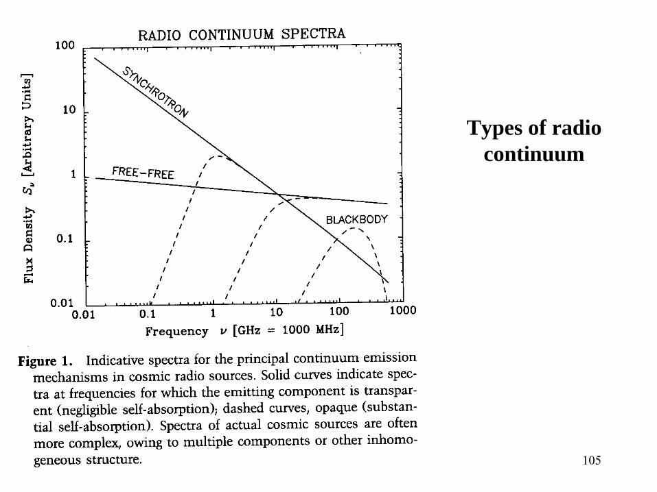
Continuum Radiation Types

• Blackbody: emission from an object in ~thermal equilibrium.• Inverse-Compton: where a photon gains energy after scattering off an

energetic electron• Synchrotron: emission from a particle moving in a magnetic field.• Free-free: (Bremsstrahlung – “braking radiation”), where unbound

protons or electrons are decelerated.• Bound-free: emission caused by ionisation and/or recombination.

96

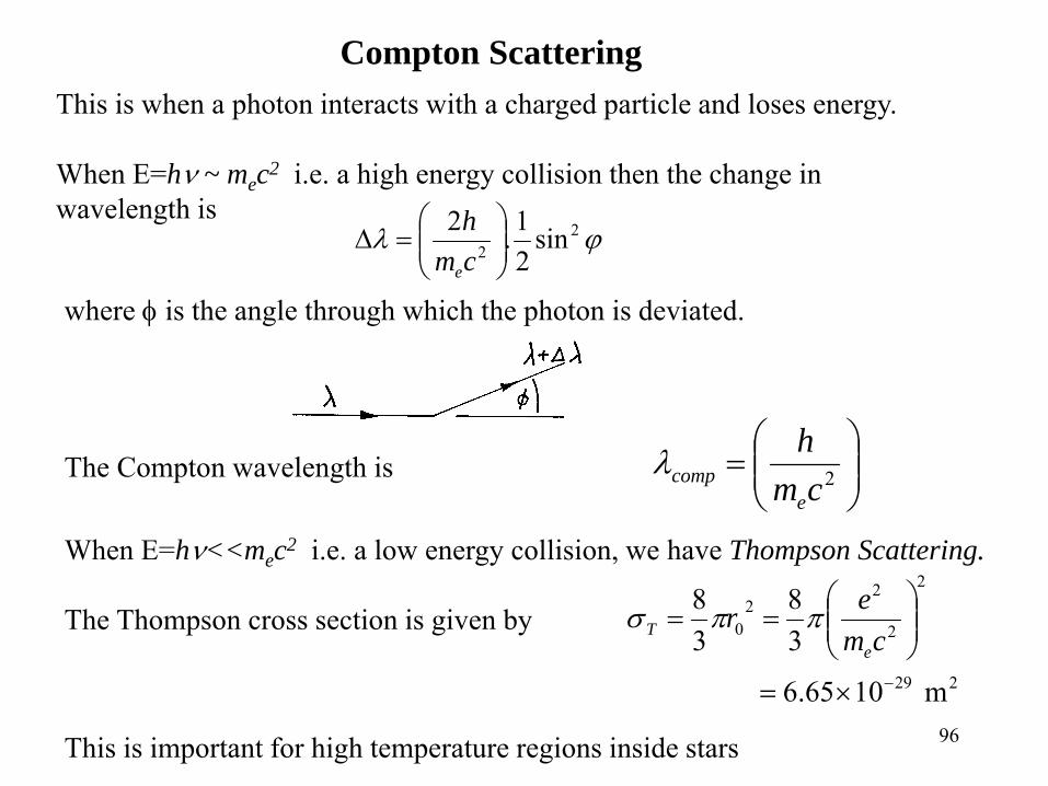
Compton Scattering

⎟⎟⎠

⎞⎜⎜⎝

⎛= 2cm

h

ecompλ

This is when a photon interacts with a charged particle and loses energy.

When E=hν ~ mec2 i.e. a high energy collision then the change in wavelength is

ϕλ 22 sin

21.2

⎟⎟⎠

⎞⎜⎜⎝

⎛=Δ

cmh

e

where φ is the angle through which the photon is deviated.

The Compton wavelength is

When E=hν<<mec2 i.e. a low energy collision, we have Thompson Scattering.

The Thompson cross section is given by

229

2

2

22

0

m1065.6

38

38

−×=

⎟⎟⎠

⎞⎜⎜⎝

⎛==

cmere

T ππσ

This is important for high temperature regions inside stars

97

Inverse-Compton Radiation

If the photon gains energy instead of losing it we create inverse-Compton radiation.

2γνν

=before

after

Where γ is the Lorentz factor of the energetic electrons that are interacting:

2

2v11c

−=γ

When γ > 103 radio waves can be shifted in frequency by more than a factor of one million. Also, optical and UV radiation can become X-ray radiation.

This is an important process in Active Galactic Nuclei (AGN).

98

Bremsstrahlung

The dominant luminous component in a cluster of galaxies is the 107 to 108 Kelvin intracluster medium. The emission from the intracluster medium is characterized by thermal Bremsstrahlung. Thermal Bremsstrahlung radiation occurs when the particles populating the emitting plasma are at a uniform temperature and are distributed according to the Maxwell–Boltzmann distribution

The bulk emission from this gas is thermal Bremsstrahlung. The power emitted per cubic centimeter per second can be written in the compact form:

where 'ff' stands for free-free, 1.4x10−27 is the condensed form of the physical constants and geometrical constants associated with integrating over the power per unit area per unit frequency, ne and ni are the electron and ion densities, respectively, Z is the number of protons of the bending charge, gB is the frequency averaged Gaunt factor and is of order unity, and T is the global x-ray temperature determined from the spectral cut-off frequency

above which exponentially small amount of photons are created because the energy required for creation of such a photon is available only for electrons in the tail of the Maxwell distribution.

99

Synchrotron Radiation-1

The force on a charge q is Bc

qEF v+=

Where E is the electric field vector, B is the magnetic field vector and v is the velocity vector. We are mostly concerned with synchrotron radiation due to electrons because they have a large charge to mass ratio, but we could also have synchrotron radiation from protons.

When the electron moves parallel to the magnetic field lines it experiences no force.

When the electron moves across the magnetic field lines it experiences a force which causes it to move in a circle.As the electron spirals in ever decreasingly smaller circles it loses energy. Combined with a component of motion along the field lines it moves along a helix with a decreasing radius. Orbital revolution has a cyclical frequency

cc v2πω =

100

Synchrotron Radiation-2

and an orbital radius of c

cr ωv

=

for relativistic electrons 22

2

2 ,

v1cmmcEm

c

mm eee γγ ===

−

=

If we equate the centrifugal force to the force from the magnetic field we have

γω

ecc

c

c

meB

meB

r

rmeBrmBe

===

=⇒=

v/v

/vv 2

In the rest frame of the electron the emitted radiation is a simple dipole. However, for a relativistic electron in the observers rest frame the radiation is “beamed” into a cone in the direction in which the electron is travelling.

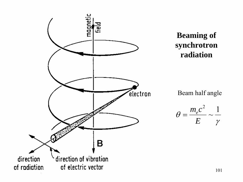
101

Beaming of synchrotron

radiation

γθ 1~

2

Ecme=

Beam half angle

102

Synchrotron Radiation-3

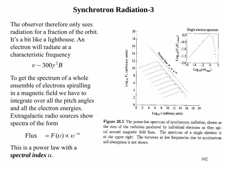
The observer therefore only sees radiation for a fraction of the orbit. It’s a bit like a lighthouse. An electron will radiate at a characteristic frequency

B2300~ γν

To get the spectrum of a whole ensemble of electrons spiralling in a magnetic field we have to integrate over all the pitch angles and all the electron energies. Extragalactic radio sources show spectra of the form

αυυ −∝= )(Flux F

This is a power law with a spectral index α.

103

Synchrotron Radiation-5

Hz110~ 3312

tBcutν

A flux distribution with a power-law form is consistent with a simple power-law distribution of electron energies.

21-with

)(βα

β

=

∝ − dEEdEEN

Typically the spectral index for radio sources is between 0.5 and 2. Synchrotron radiation can also be seen in the optical and the UV. The rate at which electrons loose energy goes as γ2 and something has to drive the process to keep it going.

Without a driving energy source the max frequency or cut-off frequency reduces with time

Below a frequency νSA the region is optically thick because electrons interact with low energy photons (they pick up energy from them). This is called synchrotron self-absorption. Below νSA we have

5.2)(Flux +∝= υυF

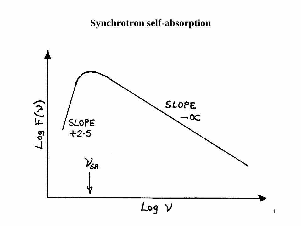
104

Synchrotron self-absorption

105

Types of radio continuum

106

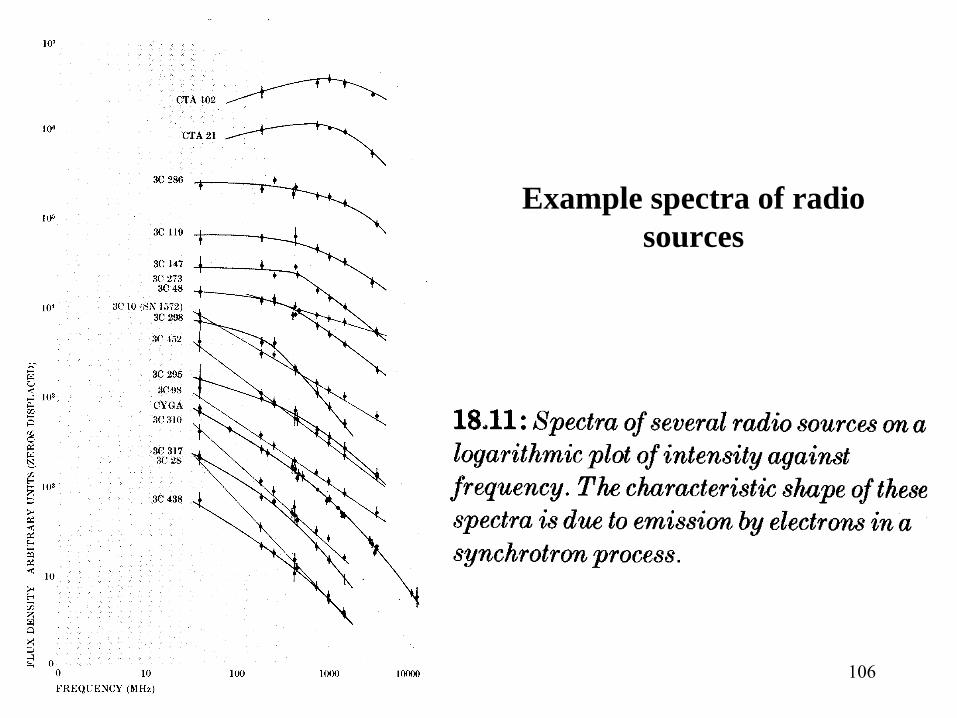
Example spectra of radio sources

107

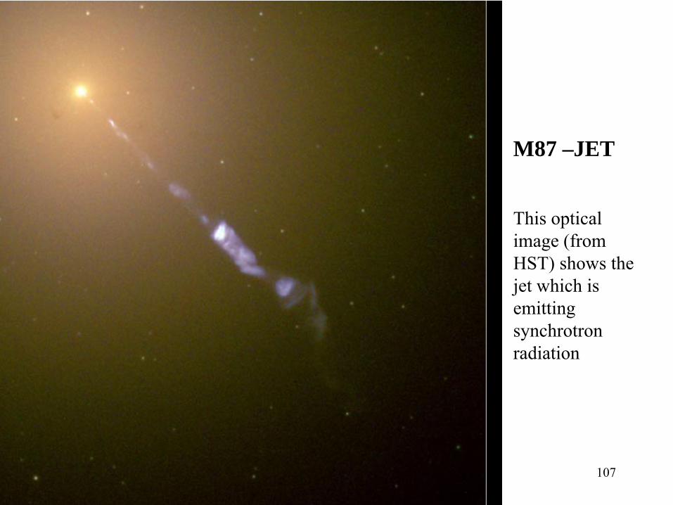
M87 –JET

This optical image (from HST) shows the jet which is emitting synchrotron radiation

108

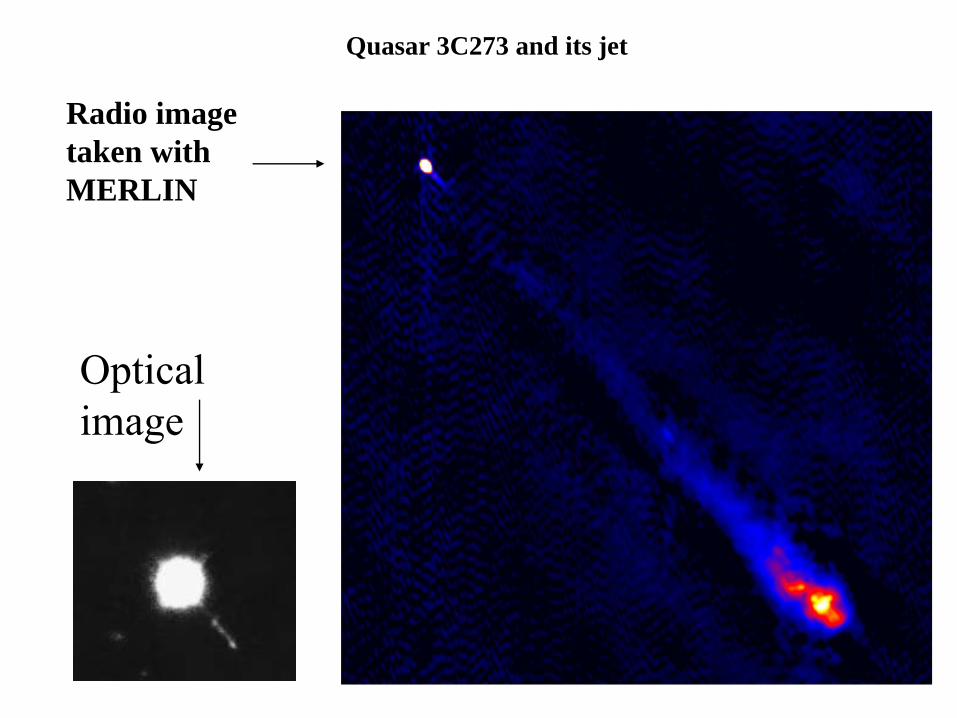
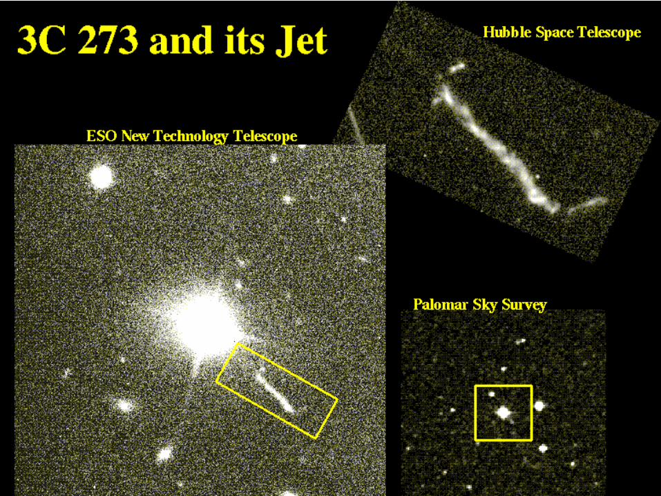
Quasar 3C273 and its jet

Radio imagetaken withMERLIN

Opticalimage

109

Quasar 3C273 and its jet

Radio imagetaken withMERLIN

Opticalimage

110

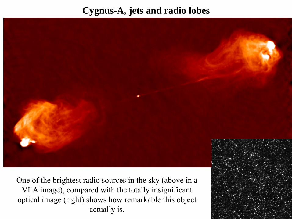
Cygnus-A, jets and radio lobes

One of the brightest radio sources in the sky (above in a VLA image), compared with the totally insignificant

optical image (right) shows how remarkable this object actually is.

111

Line spectra

• Atoms and molecules have quantized energy states.• A change between two states is associated with radiation of a

specific wavelength.• An emission line results when the atom or molecule looses energy.• An absorption line results when the atom or molecule gains

energy.• For atoms the energy levels are electronic.• For molecules the energy levels can be due to rotation and

vibration as well.• Atomic transitions have higher energies generally than molecular

ones.

Atomic transitions produce UV, optical, IR emission.Molecular transitions produce IR, mm, radio emission.

112

Transition Probabilities

• Transitions between levels follow quantum mechanical selection rules.

• Using these rules one can calculate the probability that an atom in isolation will undergo a particular (downward) transition.

• For an atom which is perturbed by a neighbour, energy can be exchanged without the absorption or emission of a photon (collisional excitation/de-excitation).

• Have to consider in any particular environment whether a collision or a transition is more likely.

113

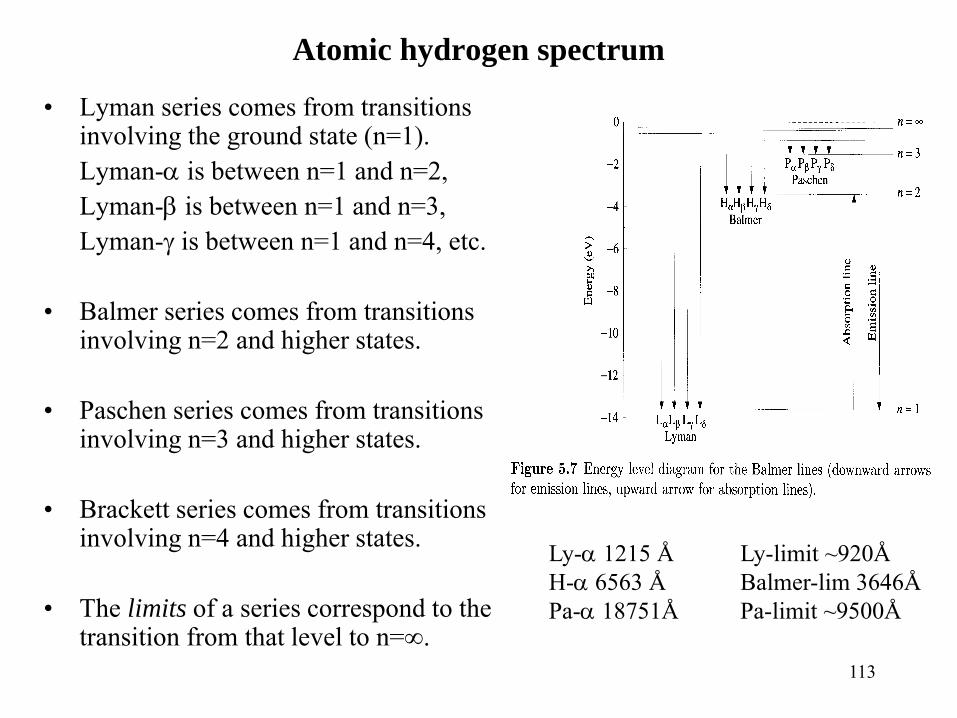
Atomic hydrogen spectrum

• Lyman series comes from transitions involving the ground state (n=1). Lyman-α is between n=1 and n=2, Lyman-β is between n=1 and n=3, Lyman-γ is between n=1 and n=4, etc.

• Balmer series comes from transitions involving n=2 and higher states.

• Paschen series comes from transitions involving n=3 and higher states.

• Brackett series comes from transitions involving n=4 and higher states.

• The limits of a series correspond to the transition from that level to n=∞.

Ly-α 1215 Å Ly-limit ~920ÅH-α 6563 Å Balmer-lim 3646ÅPa-α 18751Å Pa-limit ~9500Å

114

Terminology

• HI=H0=neutral hydrogen

• HII=H+=ionised hydrogen

• H2 is molecular hydrogen

• CIV is an ionised carbon atom with 3 electrons removed (=C+3)

• [OII] refers to a forbidden line from singly ionised oxygen, e.g. the line [OII]3727 which has a wavelength of 3727Å (372.7nm).

115

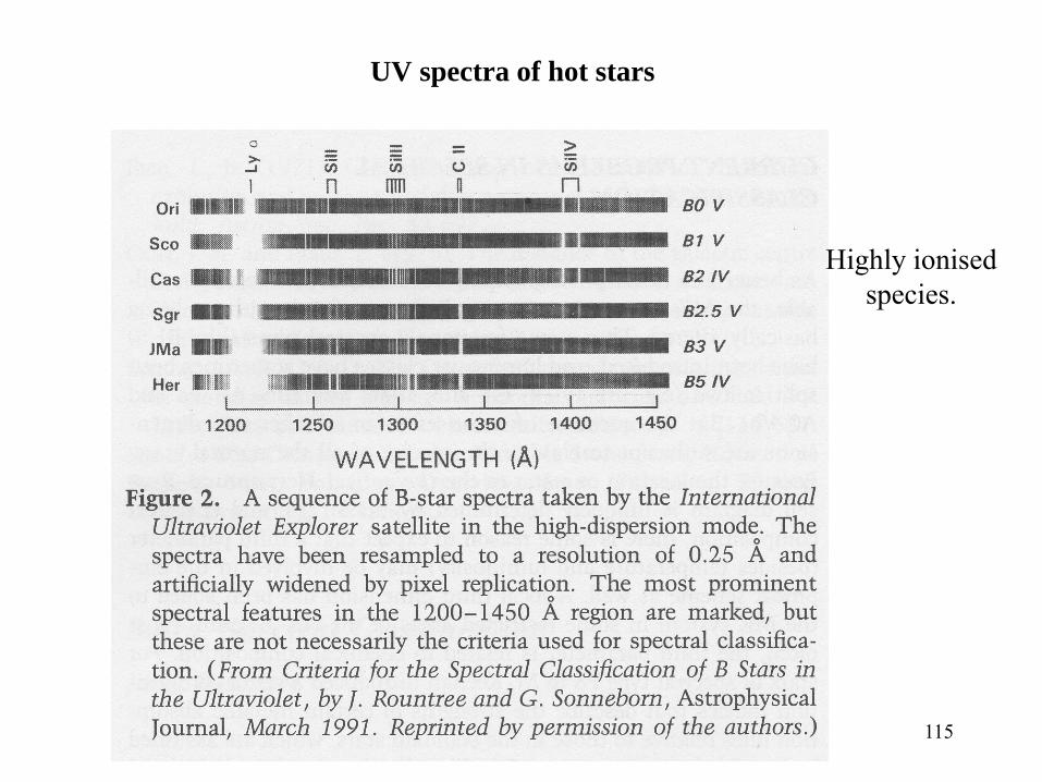
UV spectra of hot stars

Highly ionised species.

116

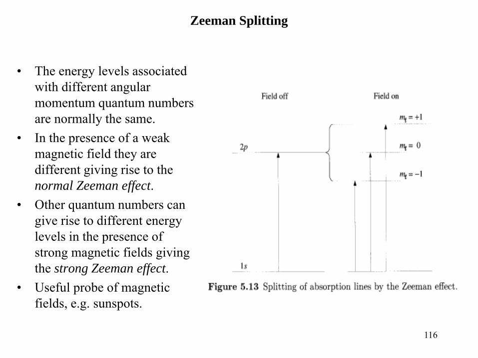
Zeeman Splitting

• The energy levels associated with different angular momentum quantum numbers are normally the same.

• In the presence of a weak magnetic field they are different giving rise to the normal Zeeman effect.

• Other quantum numbers can give rise to different energy levels in the presence of strong magnetic fields giving the strong Zeeman effect.

• Useful probe of magnetic fields, e.g. sunspots.

117

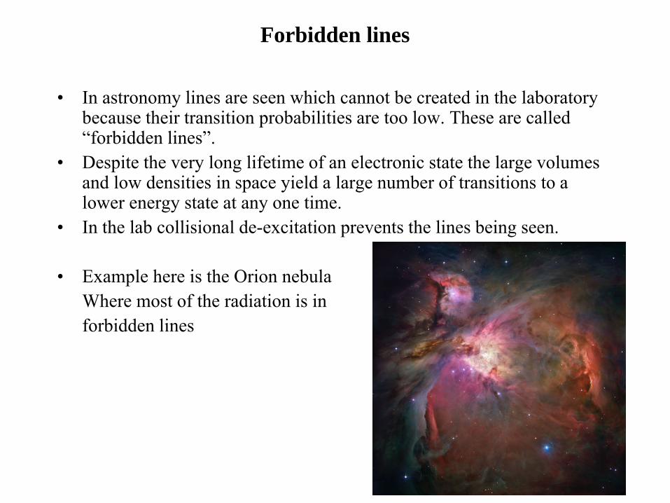
Forbidden lines

• In astronomy lines are seen which cannot be created in the laboratory because their transition probabilities are too low. These are called “forbidden lines”.

• Despite the very long lifetime of an electronic state the large volumes and low densities in space yield a large number of transitions to a lower energy state at any one time.

• In the lab collisional de-excitation prevents the lines being seen.

• Example here is the Orion nebulaWhere most of the radiation is in forbidden lines

118

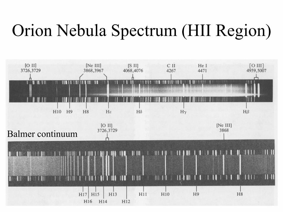
Orion Nebula Spectrum (HII Region)

Balmer continuum

119

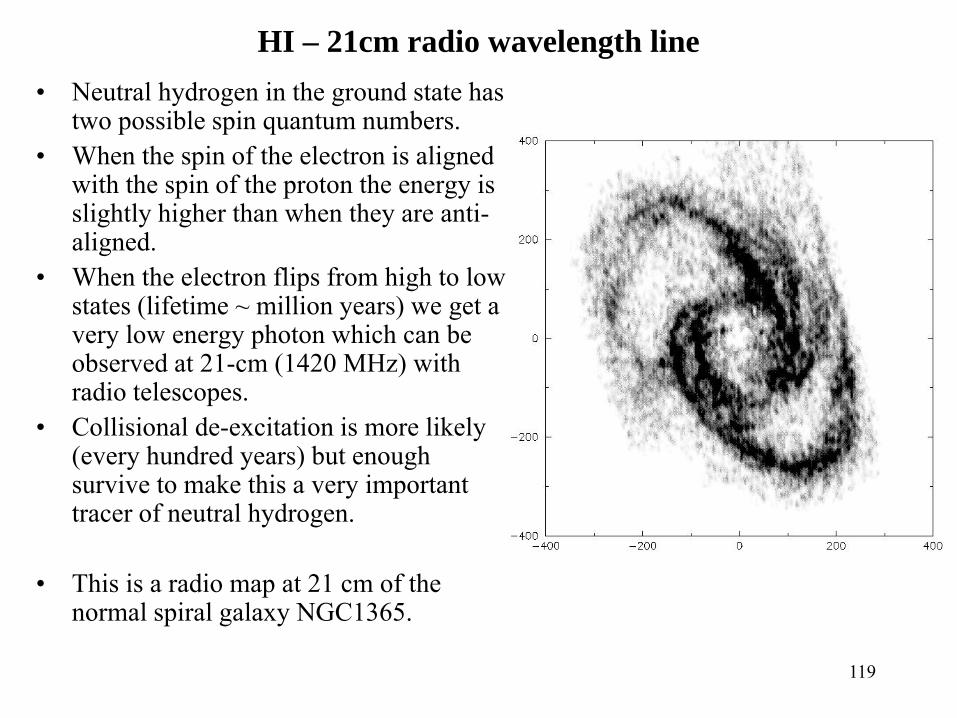
HI – 21cm radio wavelength line• Neutral hydrogen in the ground state has

two possible spin quantum numbers.• When the spin of the electron is aligned

with the spin of the proton the energy is slightly higher than when they are anti-aligned.

• When the electron flips from high to low states (lifetime ~ million years) we get a very low energy photon which can be observed at 21-cm (1420 MHz) with radio telescopes.

• Collisional de-excitation is more likely (every hundred years) but enough survive to make this a very important tracer of neutral hydrogen.

• This is a radio map at 21 cm of the normal spiral galaxy NGC1365.

120

The Milky Way

We can also trace the neutral hydrogen in our own galaxy.

This is a 21-cm map of the spiral structure of our galaxy

Sun

121

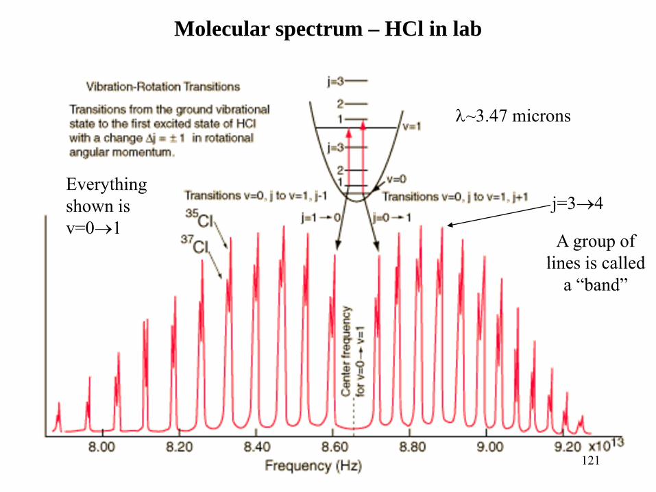
Molecular spectrum – HCl in lab

λ~3.47 microns

j=3→4Everything shown is v=0→1

A group of lines is called

a “band”

122

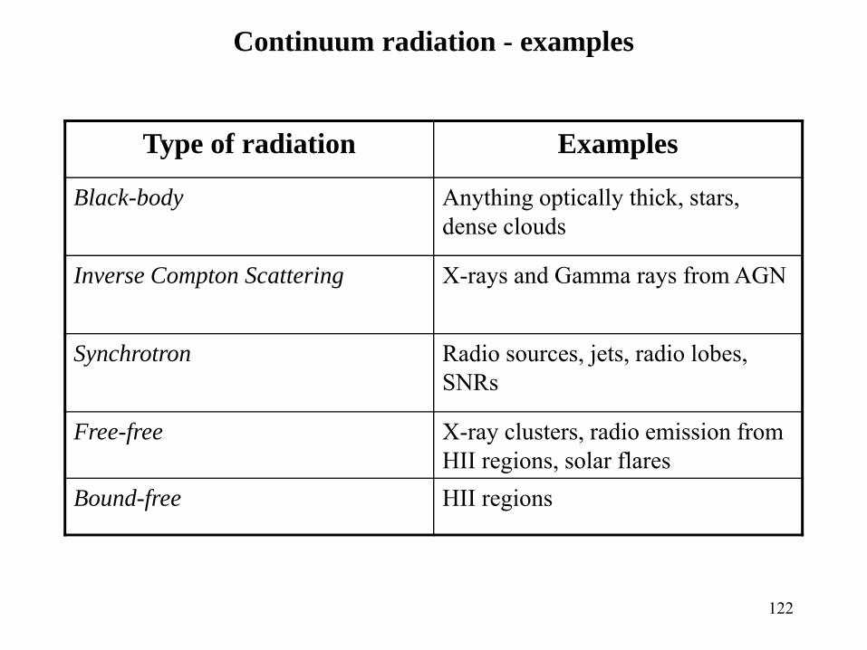
Continuum radiation - examples

Type of radiation Examples

Black-body Anything optically thick, stars, dense clouds

Inverse Compton Scattering X-rays and Gamma rays from AGN

Synchrotron Radio sources, jets, radio lobes, SNRs

Free-free X-ray clusters, radio emission from HII regions, solar flares

Bound-free HII regions

123

Stellar spectral types

• Letters denote various classes which essentially measure temperature.

• Weird sequence is a throwback to the early days of the field when they didn’t understand the underlying physics.

• Basic sequence goes O, B, A, F, G, K, M with O being the hottest and M being the coolest.

• Each class is divided into 10 subclasses, e.g. the Sun has type G2

• Brown dwarfs, Carbon stars and white dwarfs classified separately.

124

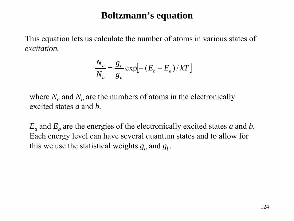
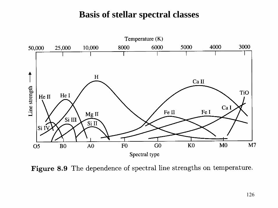
Boltzmann’s equation

This equation lets us calculate the number of atoms in various states of excitation.

[ ]kTEEgg

NN

aba

b

b

a /)(exp −−=

where Na and Nb are the numbers of atoms in the electronically excited states a and b.

Ea and Eb are the energies of the electronically excited states a and b.Each energy level can have several quantum states and to allow for this we use the statistical weights ga and gb.

125

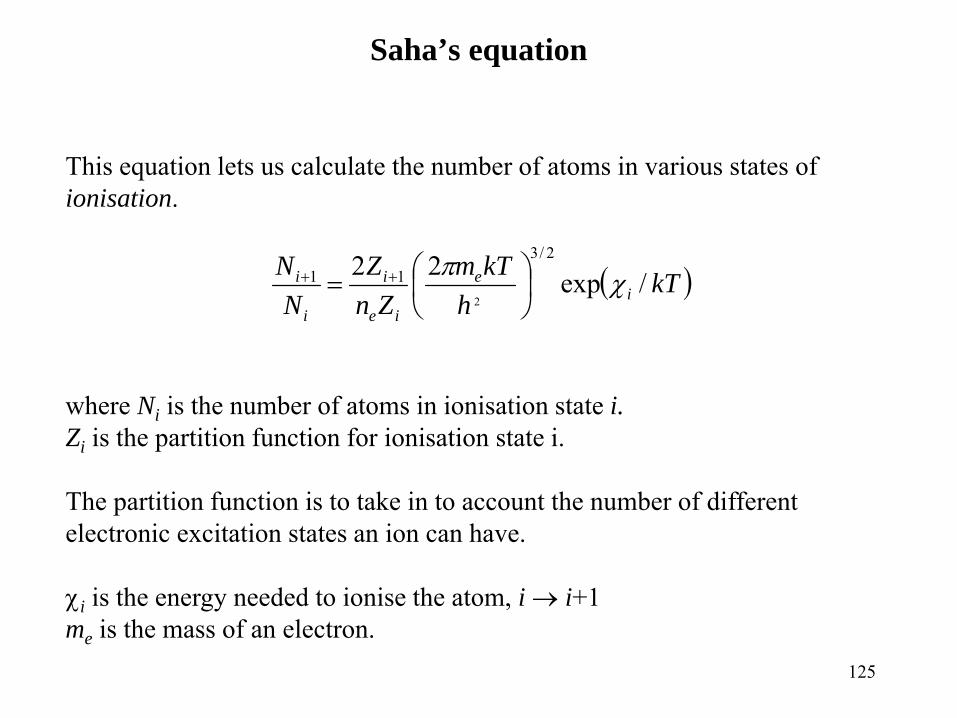
Saha’s equation

This equation lets us calculate the number of atoms in various states of ionisation.

( )kTh

kTmZn

ZN

Ni

e

ie

i

i

i /exp22 2/311

2χπ

⎟⎠⎞

⎜⎝⎛= ++

where Ni is the number of atoms in ionisation state i.Zi is the partition function for ionisation state i.

The partition function is to take in to account the number of different electronic excitation states an ion can have.

χi is the energy needed to ionise the atom, i → i+1me is the mass of an electron.

126

Basis of stellar spectral classes

127

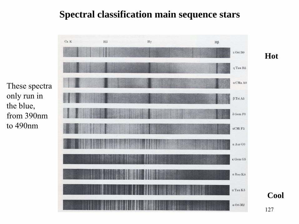
Spectral classification main sequence stars

Hot

Cool

These spectra only run in the blue, from 390nmto 490nm

128

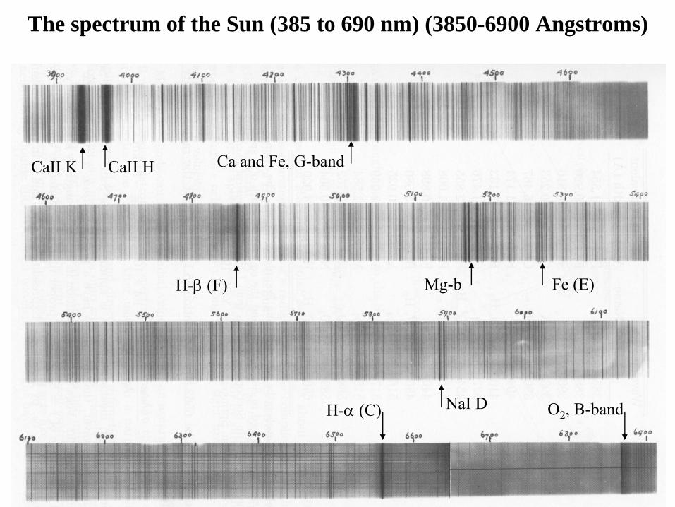
The spectrum of the Sun (385 to 690 nm) (3850-6900 Angstroms)

Ca and Fe, G-band

NaI D O2, B-bandH-α (C)

H-β (F) Mg-b

CaII HCaII K

Fe (E)

129

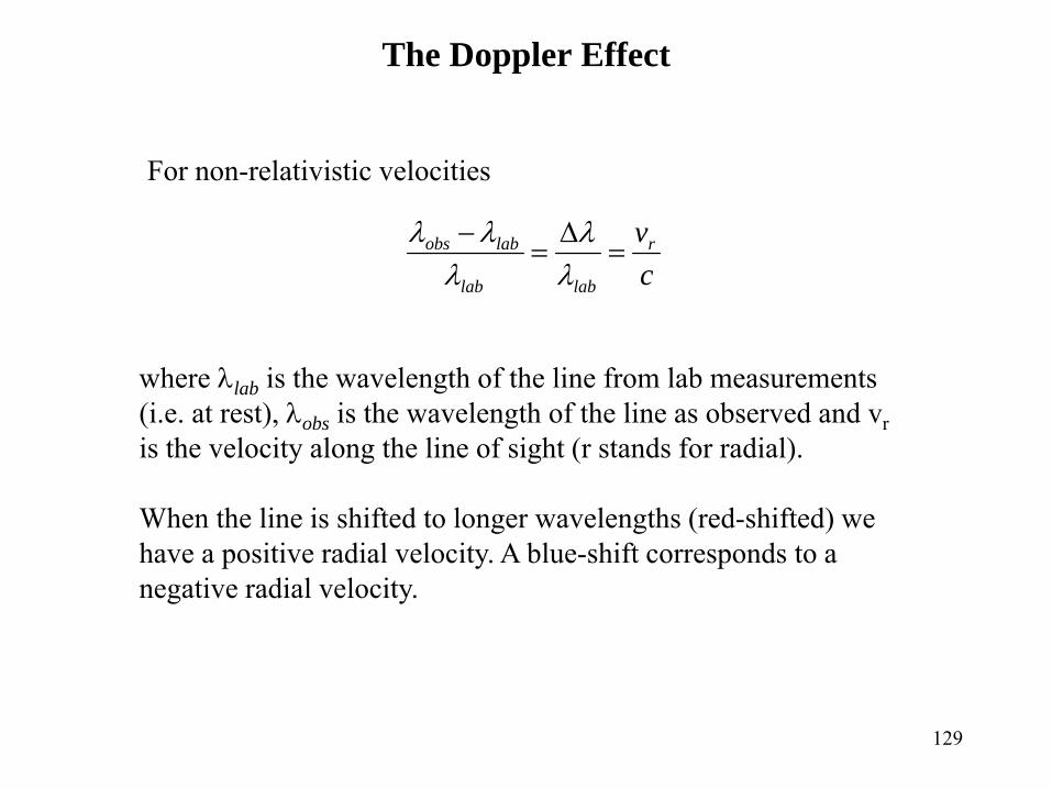
The Doppler Effect

For non-relativistic velocities

cvr

lablab

labobs =Δ

=−

λλ

λλλ

where λlab is the wavelength of the line from lab measurements (i.e. at rest), λobs is the wavelength of the line as observed and vris the velocity along the line of sight (r stands for radial).

When the line is shifted to longer wavelengths (red-shifted) we have a positive radial velocity. A blue-shift corresponds to a negative radial velocity.

130

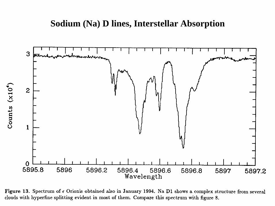
Sodium (Na) D lines, Interstellar Absorption

131

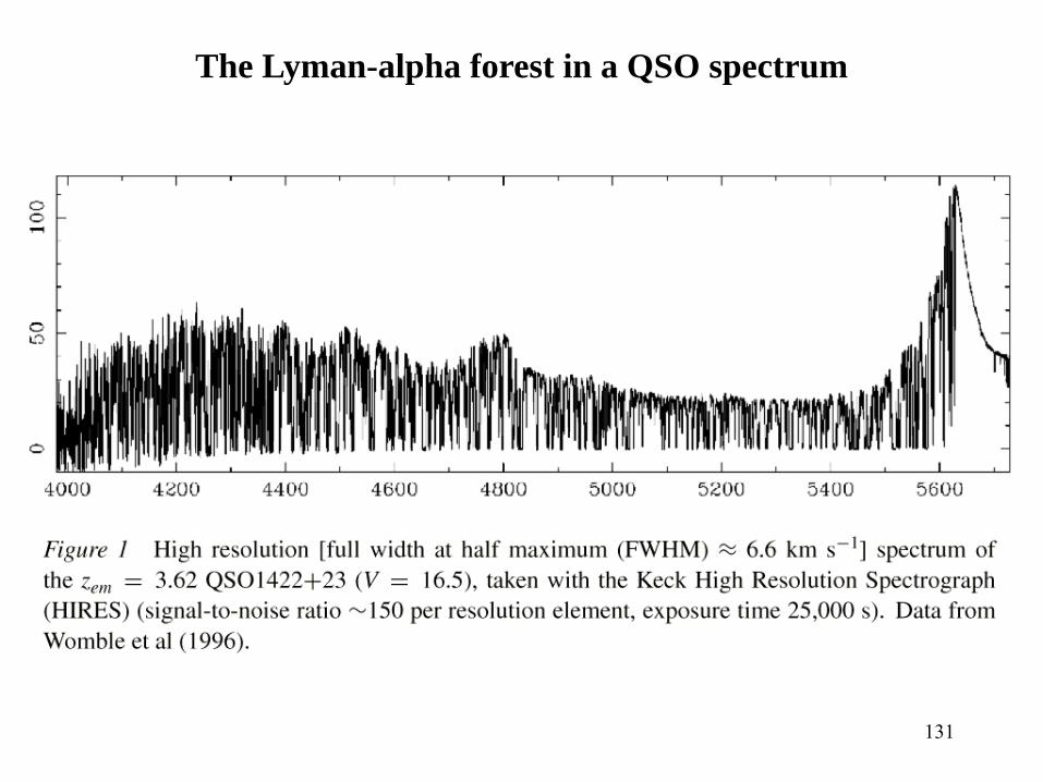
The Lyman-alpha forest in a QSO spectrum

132

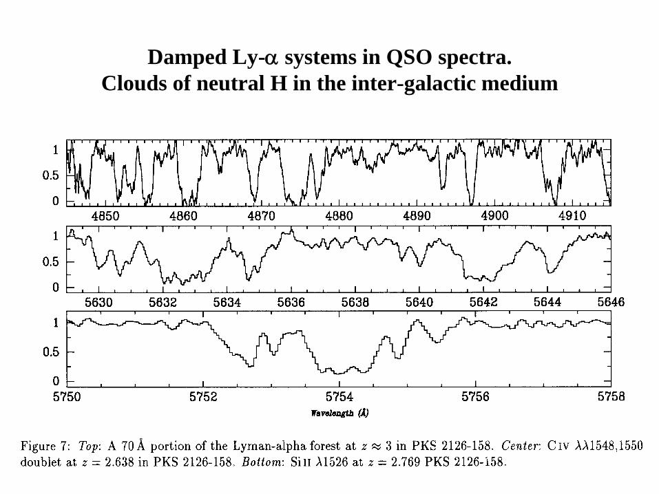
Damped Ly-α systems in QSO spectra. Clouds of neutral H in the inter-galactic medium

133

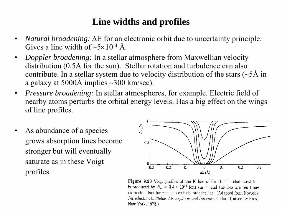
Line widths and profiles

• Natural broadening: ΔE for an electronic orbit due to uncertainty principle. Gives a line width of ~5×10-4 Å.

• Doppler broadening: In a stellar atmosphere from Maxwellian velocity distribution (0.5Å for the sun). Stellar rotation and turbulence can also contribute. In a stellar system due to velocity distribution of the stars (~5Å in a galaxy at 5000Å implies ~300 km/sec).

• Pressure broadening: In stellar atmospheres, for example. Electric field of nearby atoms perturbs the orbital energy levels. Has a big effect on the wings of line profiles.

• As abundance of a species grows absorption lines become stronger but will eventually saturate as in these Voigtprofiles.

134

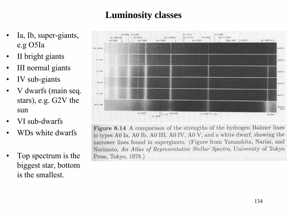
Luminosity classes

• Ia, Ib, super-giants, e.g O5Ia

• II bright giants• III normal giants• IV sub-giants• V dwarfs (main seq.

stars), e.g. G2V the sun

• VI sub-dwarfs• WDs white dwarfs

• Top spectrum is the biggest star, bottom is the smallest.

135

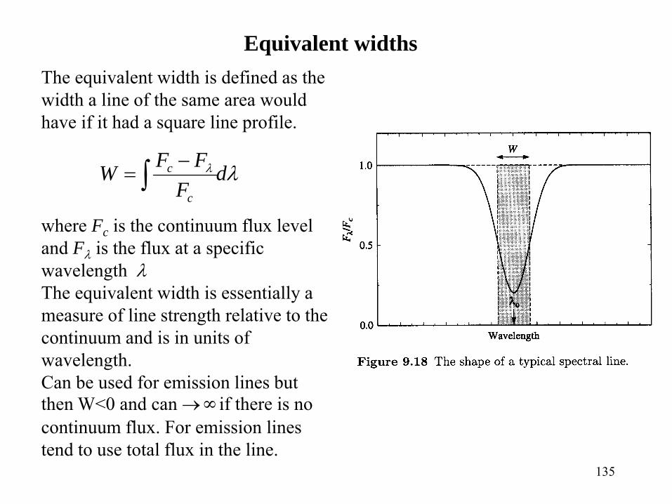
Equivalent widthsThe equivalent width is defined as the width a line of the same area would have if it had a square line profile.

λλ dF

FFWc

c∫−

=

where Fc is the continuum flux level and Fλ is the flux at a specific wavelength λThe equivalent width is essentially a measure of line strength relative to the continuum and is in units of wavelength.Can be used for emission lines but then W<0 and can →∞if there is no continuum flux. For emission lines tend to use total flux in the line.

136

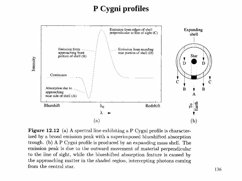
P Cygni profiles