Topics in Asset Pricing

Lecture Notes

Professor Doron Avramov

Background, Objectives, and Pre-requisite

The past few decades have been characterized by an extraordinary growth in the use

of quantitative methods in the analysis of various asset classes; be it equities, fixed

income securities, commodities, currencies, and derivatives.

In response, financial economists have routinely been using advanced mathematical,

statistical, and econometric techniques to understand asset pricing models, market

anomalies, equity premium predictability, asset allocation, security selection,

volatility, correlation, and the list goes on.

This course attempts to provide a fairly deep understanding of such topical issues.

It targets advanced master and PhD level students in finance and economics.

Required: prior exposure to matrix algebra, distribution theory, Ordinary Least

Squares, as well as kills in computer programing beyond Excel:

MATLAB, R, and Python are the most recommended for this course.

STATA or SAS are useful.

2

Topics to be covered From CAPM to market anomalies

Credit risk implications for the cross section of asset returns

Rational versus behavioural attributes of stylized cross-sectional effects

Are market anomalies pervasive?

Conditional CAPM

Conditional versus unconditional portfolio efficiency

Multi-factor models

Interpreting factor models

Panel regressions with fixed effects and their association with market-timing and cross-section investment strategies

Machine learning methods: Lasso, Ridge, elastic net, group Lasso, Neural Network, Random Forest, and adversarial GMM

Stock return predictability by macro variables

Finite sample bias in predictive regressions

Lower bound on the equity premium

The Campbell-Shiller log linearization

Consumption based asset pricing models

The discount factor representation in asset pricing

The equity premium puzzle

The risk free rate puzzle

The Epstein-Zin preferences

3

Topics to be covered Long-run risk

Habit formation

Prospect theory

Time-series asset pricing tests

Cross-section asset pricing tests

Vector auto regressions in asset pricing

On the riskiness of stocks for the long run – Bayesian perspectives

On the risk-return relation in the time series

GMM: Theory and application

The covariance matrix of regression slope estimates in the presence of heteroskedasticity and autocorrelation

Bayesian Econometrics

Bayesian portfolio optimization

The Hansen Jagannathan Distance measure

Spectral Analysis

4

Course Materials The Econometrics of Financial Markets, by John Y. Campbell, Andrew W. Lo, and A. Craig

MacKinlay, Princeton University Press, 1997

Asset Pricing, by John H. Cochrane, Princeton University Press, 2005

Class notes as well as published and working papers in finance and economics listed in the

reference list

5

From Rational Asset pricing to Market

Anomalies

6

Expected Return Statistically, an expected asset return (in excess of the risk free rate) can be formulated as

𝔼 𝑟𝑖,𝑡𝑒 = 𝛼𝑖 + 𝛽𝑖

′𝔼(𝑓𝑡)

where 𝑓𝑡 denotes a set of K portfolio spreads realized at time t, 𝛽𝑖 is a 𝐾 vector of factor loadings, and 𝛼𝑖reflects the expected return component unexplained by factors, or model mispricing.

The market model is a statistical setup with 𝑓 represented by excess return on the market portfolio.

An asset pricing model aims to identify economic or statistical factors that eliminate model mispricing.

Absent alpha, expected return differential across assets is triggered by factor loadings only.

The presence of model mispricing could give rise to additional cross sectional effects.

If factors are not return spreads (e.g., consumption growth) 𝛼 is no longer asset mispricing.

The presence of factor structure with no alpha does not imply that asset pricing is essentially rational.

Indeed, comovement of assets sharing similar styles (e.g., value, large cap) or belonging to the same

industry could be attributed to biased investor’s beliefs just as they could reflect risk premiums.

Later, we discuss in more detail ways of interpreting factor models.

7

CAPM The CAPM of Sharpe (1964), Lintner (1965), and Mossin (1966) originates the literature on asset

pricing models.

The CAPM is an equilibrium model in a single-period economy.

It imposes an economic restriction on the statistical structure of expected asset return.

The unconditional version is one where moments are time-invariant.

Then, the expected excess return on asset i is formulated as

𝔼(𝑟i,t𝑒 ) = cov(𝑟𝑖,𝑡 , 𝑟𝑚,𝑡

𝑒 )𝔼(𝑟𝑚,𝑡

𝑒 )

𝑣𝑎𝑟(𝑟𝑚,𝑡𝑒 )

= 𝛽𝑖,𝑚𝔼(𝑟𝑚,𝑡𝑒 )

where 𝑟𝑚,𝑡𝑒 is excess return on the market portfolio at time 𝑡.

Asset risk is the covariance of its return with the market portfolio return.

Risk premium, or the market price of risk, is the expected value of excess market return.

In CAPM, risk means co-movement with the market.

8

CAPM

The higher the co-movement the less desirable the asset is, hence, the asset price is lower and the

expected return is higher.

This describes the risk-return tradeoff: high risk comes along with high expected return.

The market price of risk, common to all assets, is set in equilibrium by the risk aversion of investors.

There are conditional versions of the CAPM with time-varying moments.

For one, risk and risk premium could vary with macro economy variables such as the default spread

and risk (beta) can vary with firm-level variables such as size and book-to-market.

Time varying parameters could be formulated using a beta pricing setup (e.g., Ferson and Harvey

(1999) and Avramov and Chordia (2006a)).

Another popular approach is time varying pricing kernel parameters (e.g., Cochrane (2005)).

Risk and risk premium could also obey latent autoregressive processes.

Lewellen and Nagel (LN 2006) model beta variation in rolling samples using high frequency data.

9

Empirical Violations: Market Anomalies The CAPM is simple and intuitive and it is widely used among academic scholars and

practitioners as well as in finance textbooks.

However, there are considerable empirical and theoretical drawbacks at work.

To start, the CAPM is at odds with anomalous patterns in the cross section of asset returns.

Market anomalies describe predictable patterns (beyond beta) related to firm characteristics such

as size, book-to-market, past return (short term reversals and intermediate term momentum),

earnings momentum, dispersion, net equity issuance, accruals, credit risk, asset growth, capital

investment, profitability, new 52-high, IVOL, and the list goes on.

Harvey, Liu, and Zhu (2016) document 316 (some are correlated) factors discovered by

academia.

They further propose a t-ratio of at least 3 to make a characteristic significant in cross section

regressions.

Green, Hand, and Zhang (2013) find 330 return predictive signals.

See also the survey papers of Subrahmanyam (2010) and Goyal (2012).

10

Multi-Dimension in the Cross Section? The large number of predictive characteristics leads Cochrane (2011) to conclude that there is a multi-

dimensional challenge in the cross section.

On the other hand, Avramov, Chordia, Jostova, and Philipov (2013, 2019) attribute the predictive ability of

various factors to financial distress.

They thus challenge the notion of multi-dimension in the cross section.

Their story is straightforward: firm characteristics become extreme during financial distress, such as large

negative past returns, large negative earnings surprises, large dispersion in earnings forecasts, large

volatility, and large credit risk.

Distressed stocks are thus placed in the short-leg of anomaly portfolios.

As distressed stocks keep on loosing value, anomaly profitability emerges from selling them short.

This explains the IVOL effect, dispersion, price momentum, earnings momentum, among others, all of

these effects are a manifestation of the credit risk effect.

Also, value weighting anomaly payoffs or excluding micro-cap stocks attenuate the strength of many

prominent anomalies.

The vast literature on market anomalies is briefly summarized below.

11

The Beta Effect

Friend and Blume (1970) and Black, Jensen, and Scholes (1972) show that high beta stocks deliver negative alpha, or they provide average return smaller than that predicted by the CAPM.

Frazzini and Pedersen (2014) demonstrate that alphas and Sharpe ratios are almost monotonically declining in beta among equities, bonds, currencies, and commodities.

They propose the BAB factor – a market neutral trading strategy that buys low-beta assets, leveraged to a beta of one, and sells short high-beta assets, de-leveraged to a beta of one.

The BAB factor realizes high Sharpe ratios in US and other equity markets.

What is the economic story?

For one, high beta stocks could be in high demand by constrained investors.

Moreover, Hong and Sraer (2016) claim that high beta assets are subject to speculative overpricing.

Just like the beta-return relation is counter intuitive – an apparent violation of the risk return tradeoff –there are several other puzzling relations in the cross section of asset returns.

The credit risk return relation (high credit risk low future return) is coming up next.

.

12

The credit risk return relation

Dichev (1998), Campbell, Hilscher, and Szilagyi (2008), and Avramov, Chordia, Jostova, and Philipov

(2009, 2013) demonstrate a negative cross-sectional correlation between credit risk and returns.

Campbell, Hilscher, and Szilagyi (2008) suggest that such negative relation is a challenge to standard

rational asset pricing models.

Once again, the risk-return tradeoff is challenged.

Campbell, Hilscher, and Szilagyi (2008) use failure probability estimated by a dynamic logit model with

both accounting and equity market explanatory variables.

Using the Ohlson (1980) O-score, the Z-score, or credit rating to proxy distress yields similar results.

Dichev and Piotroski (2001) and Avramov, Chordia, Jostova, and Philiphov (2009) document abnormal

stock price declines following credit rating downgrades, and further the latter study suggests that

market anomalies only characterize financially distressed firms.

On the other hand, Vassalou and Xing (2004) use the Merton’s (1974) option pricing model to compute

default measures and argue that default risk is systematic risk, and Friewald, Wagner, and Zechner

(2014) find that average returns are positively related to credit risk assessed through CDS spreads.

I believe in the negative credit risk return relation, yet the contradicting findings asks for resolution.

13

Size effect: higher average

returns on small stocks than

large stocks. Beta cannot

explain the difference. First

papers go to Banz (1981),

Basu (1983), and Fama and

French (1992)

Size Effect

14

Value effect: higher average

returns on value stocks than

growth stocks. Beta cannot

explain the difference.

Value firms: Firms with high

E/P, B/P, D/P, or CF/P. The

notion of value is that physical

assets can be purchased at low

prices.

Growth firms: Firms with low

ratios. The notion is that high

price relative to fundamentals

reflects capitalized growth

opportunities.

Value Effect

15

The International Value Effect

16

Past Return Anomalies The literature has documented short term reversals, intermediate term momentum, and long term reversals.

Lehmann (1990) and Jegadeesh (1990) show that contrarian strategies that exploit the short-run return reversals in individual stocks generate abnormal returns of about 1.7% per week and 2.5% per month, respectively.

Jegadeesh and Titman (1993) and a great body of subsequent work uncover abnormal returns to momentum-based strategies focusing on investment horizons of 3, 6, 9, and 12 months

DeBondt and Thaler (1985, 1987) document long run reversals

Momentum is the most heavily explored past return anomaly.

Several studies document momentum robustness.

Others document momentum interactions with firm, industry, and market level variables.

There is solid evidence on momentum crashes following recovery from market downturns.

More recent studies argue that momentum is attributable to the short-leg of the trade – and it difficult to implement in real time as losers stocks are difficult to short sale and arbitrage.

. 17

From Momentum Robustness to Momentum Crash Fama and French (1996) show that momentum profitability is the only CAPM-related

anomaly unexplained by the Fama and French (1993) three-factor model.

Remarkably, regressing gross momentum payoffs on the Fama-French factors tends to strengthen, rather than discount, momentum profitability.

This is because momentum loads negatively on market, size, and value factors.

Momentum also seems to appear in bonds, currencies, commodities, as well as mutual funds and hedge funds.

As Asness, Moskowitz, and Pedersen (2013) note: Momentum and value are everywhere.

Schwert (2003) demonstrates that the size and value effects in the cross section of returns, as well as the ability of the aggregate dividend yield to forecast the equity premium disappear, reverse, or attenuate following their discovery.

Momentum is an exception. Jegadeesh and Titman (2001, 2002) document the profitability of momentum strategies in the out of sample period after its initial discovery.

Haugen and Baker (1996), Rouwenhorst (1998), and Titman and Wei (2010) document momentum in international markets (not in Japan).

18

From Momentum Robustness to Momentum Crash Korajczyk and Sadka (2004) find that momentum survives trading costs, whereas

Avramov, Chordia, and Goyal (2006a) show that the profitability of short-term reversal

disappears in the presence of trading costs.

Fama and French (2008) show that momentum is among the few robust anomalies – it

works also among large cap stocks.

Geczy and Samonov (2013) examine momentum during the period 1801 through 1926 –

probably the world’s longest back-test.

Momentum had been fairly robust in a cross-industry analysis, cross-country analysis,

and cross-style analysis.

The prominence of momentum has generated both behavioral and rational theories.

Behavioral: Barberis, Shleifer, and Vishny (1998), Daniel, Hirshleifer, and

Subrahmanyam (1998), and Hon, Lim, and Stein (2000).

Rational: Berk, Green, and Naik (1999), Johnson (2002), and Avramov and Hore (2017).

19

In 2009, momentum delivers a negative 85% payoff.

The negative payoff is attributable to the short side of the trade.

Loser stocks had forcefully bounced back.

Other episodes of momentum crashes were recorded.

The down side risk of momentum can be immense.

Daniel and Moskowitz (2017) is a good empirical reference while Avramov and Hore (2017) give

theoretical support.

In addition, both Stambaugh, Yu, and Yuan (2012) and Avramov, Chordia, Jostova, and Philipov

(2007, 2013) show that momentum is profitable due to the short-leg of the trade.

Based on these studies, loser stocks are difficult to short and arbitrage – hence, it is really difficult

to implement momentum in real time.

In addition, momentum does not work over most recent years.

Momentum Crash

20

Momentum InteractionsMomentum interactions have been documented at the stock, industry, and aggregate levels.

Stock level interactions

Hon, Lim, and Stein (2000) show that momentum profitability concentrates in small stocks.

Lee and Swaminathan (2000) show that momentum payoffs increase with trading volume.

Zhang (2006) finds that momentum concentrates in high information uncertainty stocks

(stocks with high return volatility, cash flow volatility, or analysts’ forecast dispersion) and

provides behavioral interpretation.

Avramov, Chordia, Jostova, and Philipov (2007, 2013) document that momentum

concentrates in low rated stocks. Moreover, the credit risk effect seems to dominate the other

interaction effects.

Potential industry-level interactions

Moskowitz and Grinblatt (1999) show that industry momentum subsumes stock level

momentum. That is, buy the past winning industries and sell the past loosing industries.

Grundy and Martin (2001) find no industry effects in momentum. 21

Market States

Cooper, Gutierrez, and Hameed (2008) show that momentum profitability heavily depends on the state of the market.

In particular, from 1929 to 1995, the mean monthly momentum profit following positive market returns is 0.93%, whereas the mean profit following negative market return is -0.37%.

The study is based on the market performance over three years prior to the implementation of the momentum strategy.

Market sentiment Antoniou, Doukas, and Subrahmanyam (2010) and Stambaugh, Yu, and Yuan (2012) find that

the momentum effect is stronger when market sentiment is high.

The former paper suggests that this result is consistent with the slow spread of bad news during high-sentiment periods.

Stambaugh, Yu, and Yuan (2015) use momentum along with ten other anomalies to form a stock level composite overpricing measure. For instance, loser stocks are likely to be overpriced due to impediments on short selling.

22

Other interactions at the aggregate level Chordia and Shivakumar (2002) show that momentum is captured by business cycle variables.

Avramov and Chordia (2006a) demonstrate that momentum is captured by the component in model mispricing that varies with business conditions.

Avramov, Cheng, and Hameed (2016) show that momentum payoffs vary with market illiquidity - in contrast to “limits to arbitrage” momentum is profitable during highly liquid markets.

Momentum in Anomalies Avramov et al (Scaling Up Market Anomalies 2017) show that one could implement momentum among top and

bottom anomaly portfolios.

They consider 15 market anomalies, each of which is characterized by the anomaly conditioning variable., e.g., gross profitability, IVOL, and dispersion in analysts earnings forecast.

There are 15 top (best performing long-leg) portfolios.

There are 15 bottom (worst performing short-leg) portfolios.

The trading strategy involves buying a subset (e.g., five) top portfolios and selling short a subset of bottom portfolios based on past one-month return or based on expected return estimated from time-series predictive regressions.

Implementing momentum among anomalies delivers a robust performance even during the post-2000 period and during periods of low market sentiment.

Building on Avramov et al (2017), Eshani and Linnainmaa (2019) show that stock-level momentum emerges from momentum in factor returns.

Thus, momentum is not a distinct risk factor; rather, it aggregates the autocorrelations found in all other factors.

23

Momentum Spillover from Stocks to Bonds Gebhardt, Hvidkjaer, and Swaminathan (2005) examine the interaction between momentum in the

returns of equities and corporate bonds.

They find significant evidence of a momentum spillover from equities to corporate bonds of the same

firm.

In particular, firms earning high (low) equity returns over the previous year earn high (low) bond

returns in the following year.

The spillover results are stronger among firms with lower-grade debt and higher equity trading

volume.

Beyond momentum spillover, Jostova et al (2013) find significant price momentum in US corporate

bonds over the 1973 to 2008 period.

They show that bond momentum profits are significant in the second half of the sample period, 1991

to 2008, and amount to 64 basis points per month.

24

Are there Predictable Patterns in Corporate Bonds? For the most part, anomalies that work on equities also work on corporate bonds.

In addition, the same-direction mispricing applies to both stocks and bonds.

See, for example, Avramov, Chordia, Jostova, and Philipov (2019).

They document overpricing in stocks and corporate bonds.

Indeed, structural models of default, such as that originated by Merton (1974), impose a tight relation between

equity and bond prices, as both are claims on the same firm assets.

Then, if a characteristic x is able to predict stock returns, it must predict bond returns.

On one hand, the empirical question is thus whether bond returns are over-predictable or under-predictable for a

given characteristic.

On the other hand, structural models of default have had difficult times to explain credit spreads and moreover

bond and stock markets may not be integrated.

Also, some economic theory claims that there might be wealth transfer from bond holders to equity holders –

thus, one may suspect that equity overpricing must be followed by bond underpricing.

25

Time-Series Momentum Time-series momentum in an absolute strength strategy, while the price momentum is a

relative strength one. Here, one takes long positions in those stocks having positive expected

returns and short positions in stocks having negative expected returns, where expected

return is assessed based on the following equation from Moskowitz, Ooi, and Pedersen (2012):

Τ𝑟𝑡𝑠 𝜎𝑡−1

𝑠 = 𝛼 + Τ𝛽ℎ𝑟𝑡−ℎ𝑠 𝜎𝑡−ℎ−1

𝑠 + 휀𝑡𝑠

Earnings Momentum (see also next page) Ball and Brown (1968) document the post-earnings-announcement drift, also known as

earnings momentum.

This anomaly refers to the fact that firms reporting unexpectedly high earnings subsequently

outperform firms reporting unexpectedly low earnings.

The superior performance lasts for about nine months after the earnings announcements.

Revenue Momentum Chen, Chen, Hsin, and Lee (2010) study the inter-relation between price momentum, earnings

momentum, and revenue momentum, concluding that it is ultimately suggested to combine all

types rather than focusing on proper subsets.

26

Earnings Momentum: under-reaction?

27

Asset Growth Cooper, Gulen, and Schill (2008) find companies that grow their total asset more earn lower

subsequent returns.

They suggest that this phenomenon is due to investor initial overreaction to changes in future business prospects implied by asset expansions.

Asset growth can be measured as the annual percentage change in total assets.

Capital Investment Titman, Wei, and Xie (2004) document a negative relation between capital investments and

returns.

Capital investment to assets is the annual change in gross property, plant, and equipment plus the annual change in inventories divided by lagged book value of assets.

Changes in property, plants, and equipment capture capital investment in long-lived assets used in operations many years such as buildings, machinery, furniture, and other equipment.

Changes in inventories capture working capital investment in short-lived assets used in a normal business cycle.

28

Idiosyncratic volatility (IVOL)

Ang, Hodrik, Xing, and Zhang (2006, 2009) show negative cross section relation between IVOL and average

return in both US and global markets.

The AHXZ proxy for IVOL is the standard deviation of residuals from time-series regressions of excess stock

returns on the Fama-French factors.

Counter intuitive relations

The forecast dispersion, credit risk, betting against beta, and IV effects apparently violate the risk-return

tradeoff.

Investors seem to pay premiums for purchasing higher risk stocks.

Intuition may suggest it should be the other way around.

Avramov, Chordia, Jostova, and Philipov (2013, 2018) provide a plausible story: institutional and retail

investors underestimate the severe implications of financial distress.

Thus, financially distressed stocks (and bonds) are overpriced.

As financially distressed firms exhibit high IVOL, high beta, high credit risk, and high dispersion – all the

counter intuitive relations are explained by the overpricing of financially distressed stocks.

29

Return on Assets (ROA) Fama and French (2006) find that more profitable firms (ROA) have higher expected returns than

less profitable firms.

ROA is typically measured as income before extraordinary items divided by one quarter lagged

total assets.

Quality Investing Novy-Marks describes seven of the most widely used notions of quality:

Sloan’s (1996) accruals-based measure of earnings quality (coming next)

Measures of information uncertainty and financial distress (coming next)

Novy-Marx’s (2013) gross profitability (coming next)

Piotroski’s (2000) F-score measure of financial strength (coming next)

Graham’s quality criteria from his “Intelligent Investor” (appendix)

Grantham’s “high return, stable return, and low debt” (appendix)

Greenblatt’s return on invested capital (appendix)

30

Accruals: Sloan (1996) shows that firms with high accruals earn abnormal lower returns on

average than firms with low accruals. Sloan suggests that investors overestimate the persistence

of the accrual component of earnings when forming earnings expectations. Total accruals are

calculated as changes in noncash working capital minus depreciation expense scaled by average

total assets for the previous two fiscal years.

Information uncertainty: Diether, Malloy, and Scherbina (2002) suggest that firms with high

dispersion in analysts’ earnings forecasts earn less than firms with low dispersion. Other

measures of information uncertainty: firm age, cash flow volatility, etc.

Financial distress: As noted earlier, Campbell, Hilscher, and Szilagyi (2008) find that firms

with high failure probability have lower, not higher, subsequent returns. Campbell, Hilscher, and

Szilagyi suggest that their finding is a challenge to standard models of rational asset pricing. The

failure probability is estimated by a dynamic logit model with both accounting and equity market

variables as explanatory variables. Using Ohlson (1980) O-score as the distress measure yields

similar results. Avramov, Chordia, Jostova, and Philipov (2009) use credit ratings as a proxy for

financial distress and also document the same phenomenon: higher credit rating firms earn

higher returns than low credit rating firms.

Quality investing: Accruals, Information uncertainty, and Distress

31

Quality investing: Gross Profitability Premium Novy-Marx (2010) discovers that sorting on gross-profit-to-assets creates abnormal benchmark-

adjusted returns, with more profitable firms having higher returns than less profitable ones.

Novy-Marx argues that gross profits scaled by assets is the cleanest accounting measure of true

economic profitability. The further down the income statement one goes, the more polluted

profitability measures become, and the less related they are to true economic profitability.

Quality investing: F-Score The F-Score is due to Piotroski (2000).

It is designed to identify firms with the strongest improvement in their overall financial conditions

while meeting a minimum level of financial performance.

High F-score firms demonstrate distinct improvement along a variety of financial dimensions, while

low score firms exhibit poor fundamentals along these same dimensions.

F-Score is computed as the sum of nine components which are either zero or one.

It thus ranges between zero and nine, where a low (high) score represents a firm with very few

(many) good signals about its financial conditions.

32

Illiquidity Illiquidity is not considered to be an anomaly.

However, it is related to the cross section of average returns (as well as the time-series)

Amihud (2002) proposes an illiquidity measure which is theoretically appealing and does a good job empirically.

The Amihud measure is given by:

𝐼𝐿𝐿𝐼𝑄𝑖,𝑡 =1

𝐷𝑖,𝑡

𝑡=1

𝐷𝑖,𝑡 𝑅𝑖𝑡𝑑𝐷𝑉𝑂𝐿𝑖𝑡𝑑

where: 𝐷𝑖,𝑡 is the number of trading days in the month, 𝐷𝑉𝑂𝐿𝑖𝑡𝑑 is the dollar volume, 𝑅𝑖𝑡𝑑 is

the daily return

The illiquidity variable measures the price change per a unity volume.

Higher change amounts to higher illiquidity

33

The turnover effect

Higher turnover is followed by lower future return. See, for example, Avramov and Chordia

(2006a).

Swaminathan and Lee (2000) find that high turnover stocks exhibit features of high growth stocks.

Turnover can be constructed using various methods. For instance, for any trading day within a

particular month, compute the daily volume in either $ or the number of traded stocks or the

number of transactions. Then divide the volume by the market capitalization or by the number of

outstanding stocks. Finally, use the daily average, within a trading month, of the volume/market

capitalization ratio as the monthly turnover.

Economic links and predictable returns

Cohen and Frazzini (2008) show that stocks do not promptly incorporate news about economically

related firms.

A long-short strategy that capitalizes on economic links generates about 1.5% per month.

34

Corporate Anomalies The corporate finance literature has documented a host of other interesting anomalies:

Stock Split

Dividend initiation and omission

Stock repurchase

Spinoff

Merger arbitrage

The long horizon performance of IPO and SEO firms.

Finance research has documented negative relation between transactions of external

financing and future stock returns: returns are typically low following IPOs (initial

public offerings), SEOs (seasoned public offerings), debt offerings, and bank borrowings.

Conversely, future stock returns are typically high following stock repurchases.

See also discussion in the appendix.

35

Are anomalies pervasive? The evidence tilts towards the NO answer. Albeit, the tilt is not decisive.

Lo and MacKinlay (1990) claim that the size effect may very well be the result of unconscious, exhaustive search for a portfolio formation creating with the aim of rejecting the CAPM.

Schwert (2003) shows that anomalies (time-series and cross section) disappear or get attenuated following their discovery.

Avramov, Chordia, and Goyal (2006) show that implementing short term reversal strategies yields profits that do not survive direct transactions costs and costs related to market impact.

Wang and Yu (2010) find that the return on asset (ROA) anomaly exists primarily among firms with high arbitrage costs and high information uncertainty.

Avramov, Chordia, Jostova, and Philipov (2007a,b, 2013, 2019) show that momentum, dispersion, credit risk, among many other effects, concentrate in a very small portion of high credit risk stocks and only during episodes of firm financial distress.

In particular, investors tend to overprice distressed stocks. Moreover, distressed stocks display extreme values of firm characteristics – high IVOL, high dispersion, large negative past returns, and large negative earnings surprises. They are thus placed at the short-leg of anomaly portfolios. Anomaly profitability emerges only from the short-leg of a trade, as overpricing is corrected.

36

Are anomalies pervasive? Chordia, Subrahmanyam, and Tong (2014) and McLean and Pontiff (2014) find that several

anomalies have attenuated significantly over time, particularly in liquid NYSE/AMEX stocks, and

virtually none have significantly accentuated.

Stambaugh, Yu, and Yuan (2012) associate anomalies with market sentiment.

Following Miller (1977), there might be overpriced stocks due to costly short selling.

As overpricing is prominent during high sentiment periods, anomalies are profitable only during

such episodes and are attributable to the short-leg of a trade.

Avramov, Chordia, Jostova, and Philipov (2013) and Stambaugh, Yu, and Yuan (2012) seem to

agree that anomalies represent an un-exploitable stock overvaluation.

But the sources are different: market level sentiment versus firm-level credit risk.

Avramov, Chordia, Jostova, and Philipov (2019) integrate the evidence: anomalies concentrate in

the intersection of firm credit risk and market-wide sentiment.

And the same mechanism applies for both stocks and corporate bonds.

Beyond Miller (1977), there are other economic theories that permit overpricing.

37

Are anomalies pervasive? For instance, the Harrison and Kreps (1978) basic insight is that when agents agree to disagree and short

selling is impossible, asset prices may exceed their fundamental value.

The positive feedback economy of De Long, Shleifer, Summers, and Waldmann (1990) also recognizes the possibility of overpricing ─ arbitrageurs do not sell or short an overvalued asset, but rather buy it, knowing that the price rise will attract more feedback traders.

Garlappi, Shu, and Yan (2008) and Garlappi and Yan (2011) argue that distressed stocks are overvalued due to shareholders' ability to extract value from bondholders during bankruptcy.

Kumar (2009), Bailey, Kumar, and Ng (2011), and Conrad, Kapadia, and Xing (2014) provide support for lottery-type preferences among retails investors. Such preferences can also explain equity overpricing.

Lottery-type stocks are stocks with low price, high idiosyncratic volatility, and positive return skewness.

The idea of skewness preferring investors goes back to Barberis and Huang (2008) who build on the prospect theory of Kahneman and Tversky (1979) to argue that overpricing could prevail as investors overweight low-probability windfalls.

Notice, however, that Avramov, Chordia, Jostova, and Philipov (2019) find that bonds of overpriced equity firms are also overpriced, thus calling into question the transfer of wealth hypothesis.

Also, the upside potential of corporate bonds is limited relative to that of stocks – thus lottery-type preferences are less likely to explain bond overpricing.

In sum, anomalies do not seem to be pervasive. They could emerge due to data mining, they typically characterize the short-leg of a trade, they concentrate in difficult to short and arbitrage stocks, and they might fail survive reasonable transaction costs.

38

Could anomalies emerge from the long-leg? Notably, some work does propose the possibility of asset underpricing.

Theoretically, in Diamond and Verrecchia (1987), investors are aware that, due to short sale constraints, negative information is withheld, so individual stock prices reflect an expected quantity of bad news. Prices are correct, on average, in the model, but individual stocks can be overvalued or undervalued.

Empirically, Boehmer, Huszar, and Jordan (2010) show that low short interest stocks exhibit positive abnormal returns. Short sellers avoid those apparently underpriced stocks

Also, the 52-week high anomaly tells you that stocks that are near their 52-week high are underpriced.

Recently, Avramov, Kaplanski, and Subrahmanyam (2018) show that a ratio of short (fast) and long (slow) moving averages predict both the long and short legs of trades.

The last two papers attribute predictability to investor’s under-reaction due to the anchoring bias.

Avramov, Kaplanski, and Subrahmanyam (2019) show theoretically why anchoring could result in positive autocorrelation in returns.

The anchoring bias is the notion that agents rely too heavily on readily obtainable (but often irrelevant) information in forming assessments (Tversky and Kahneman, 1974).

39

Sticky expectations and market anomalies

As an example of the anchoring bias, in Ariely, Loewenstein, and Prelec (2003), participants are asked to write the last two digits of their social security number and then asked to assess how much they would pay for items of unknown value. Participants having lower numbers bid up to more than double relative to those with higher numbers, indicating that they anchor on these two numbers.

Such under-reaction could be long lasting as shown by Avramov, Kaplanski, and Subrahmanyam (2019).

While the former study points at anchoring as a potential rationale for mispricing, the sticky expectations (SE) concept somehow formalizes the same notion.

The SE concept has been developed and studied by Mankiw and Reis (2002), Reis (2006), and Coibion and Gorodnichenko (2012, 2015).

Bouchaus, Kruger, Landier, and Thesmar (2019) propose SE to explain the profitability anomaly along with price momentum and earnings momentum.

The idea is straightforward.

In particular, expectations about an economic quantity (πt+h) are updated using the process

𝐹𝑡πt+h = 1 − 𝜆 𝐸𝑡πt+h+ 𝜆𝐹𝑡−1πt+h

40

Sticky expectations and market anomalies

The term 𝐸𝑡πt+h denotes the rational expectation of πt+h conditional on information

available at date t.

The coefficient λ indicates the extent of expectation stickiness.

When λ = 0, expectations are perfectly rational.

Otherwise, new information is insufficiently accounted for in establishing forecasts.

This framework accommodates patterns of both under-reaction (0 < λ < 1) and

overreaction (λ < 0).

As noted by Coibion and Gorodnichenko (2012, 2015), this structure gives rise to

straightforward testable predictions that are independent of the process underlying

πt+h.

This structure also provides a direct measure of the level of stickiness.

41

Sticky expectations and market anomalies

In the first place, forecast errors should be predicted by past revisions:

𝐸𝑡 πt+1−𝐹𝑡πt+1 =λ

1 − λ𝐹𝑡πt+1−𝐹𝑡−1πt+1

Second, revisions are auto-correlated over time:

𝐸𝑡−1 𝐹𝑡πt+1 −𝐹𝑡−1πt+1 =λ 𝐹𝑡−1πt+1−𝐹𝑡−2πt+1

These two relations can be readily tested on expectations data (including inflation, profitability, interest rate, future price) without further assumptions about the data-generating process of π.

The intuition behind the first testable restriction is that forecast revisions contain some element of new information that is only partially incorporated into expectations.

The second prediction pertains to the dynamics of forecast revisions.

When expectations are sticky, information is slowly incorporated into forecasts, so that positive news generates positive forecast revisions over several periods.

This generates momentum in forecasts.

42

Market Anomalies: Polar Views Scholars like Fama would claim that the presence of anomalies merely indicates the

inadequacy of the CAPM.

Per Fama, an alternative risk based model would capture all anomalous patterns in asset

prices. Markets are in general efficient and the risk-return tradeoff applies. The price is right

up to transaction cost bounds.

Scholars like Shiller would claim that asset prices are subject to behavioral biases.

Per Shiller, asset returns are too volatile to be explained by changing fundamental values and

moreover higher risk need not imply higher return.

Both Fama and Shiller won the Nobel Prize in Economics in 2013.

Fama and Shiller represent polar views on asset pricing: rational versus behavioral.

But whether or not markets are efficient seems more like a philosophical question.

In his presidential address, Cochrane (2011) nicely summarizes this debate. See next page.

43

Rational versus Behavioral perspectives It is pointless to argue “rational” vs. “behavioral.”

There is a discount rate and equivalent distorted probability that can rationalize any

(arbitrage-free) data.

“The market went up, risk aversion must have declined” is as vacuous as “the market

went up, sentiment must have increased.” Any model only gets its bite by restricting

discount rates or distorted expectations, ideally tying them to other data.

The only thing worth arguing about is how persuasive those ties are in a given model

and dataset.

And the line between recent “exotic preferences” and “behavioral finance” is so blurred, it

describes academic politics better than anything substantive.

For example, which of Epstein and Zin (1989), Barberis, Huang, and Santos (2001),

Hansen and Sargent (2005), Laibson (1997), Hansen, Heaton and Li (2008), and

Campbell and Cochrane (1999) is really “rational” and which is really “behavioral?

Changing expectations of consumption 10 years from now (long run risks) or changing

probabilities of a big crash are hard to tell from changing “sentiment.”

44

Rational versus Behavioral perspectives Yet another intriguing quote followed by a response.

Cochrane (2011): Behavioral ideas - narrow framing, salience of recent experience, and so forth - are good at generating anomalous prices and mean returns in individual assets or small groups. They do not easily generate this kind of coordinated movement across all assets that looks just like a rise in risk premium. Nor do they naturally generate covariance. For example, “extrapolation” generates the slight autocorrelation in returns that lies behind momentum. But why should all the momentum stocks then rise and fall together the next month, just as if they are exposed to a pervasive, systematic risk?

Kozak, Nagel, and Stantosh (KNS 2017a): The answer to this question could be that some components of sentiment-driven asset demands are aligned with covariances with important common factors, some are orthogonal to these factor covariances. Trading by arbitrageurs eliminates the effects of the orthogonal asset demand components, but those that are correlated with common factor exposures survive because arbitrageurs are not willing to accommodate these demands without compensation for the factor risk exposure.

45

Theoretical Drawbacks of the CAPM

A. The CAPM assumes that the average investor cares only about the performance of the

investment portfolio.

But eventual wealth could emerge from both investment, labor, and entrepreneurial incomes.

Additional factors are therefore needed.

The CAPM says that two stocks that are equally sensitive to market movements must have the

same expected return.

But if one stock performs better in recessions it would be more desirable for most investors who

may actually lose their jobs or get lower salaries in recessions.

The investors will therefore bid up the price of that stock, thereby lowering expected return.

Thus, pro-cyclical stocks should offer higher average returns than countercyclical stocks, even if

both stocks have the same market beta.

Put another way, co-variation with recessions seems to matter in determining expected returns.

You may correctly argue that the market tends to go down in recessions.

Yet, recessions tend to be unusually severe or mild for a given level of market returns.46

ICAPMB. The CAPM assumes a static one-period model.

Merton (1973) introduces a multi-period version of the CAPM - the inter-temporal CAPM

(ICAPM).

In ICAPM, the demand for risky assets is attributed not only to the mean variance component, as

in the CAPM, but also to hedging against unfavorable shifts in the investment opportunity set.

The hedging demand is something extra relative to the CAPM.

In ICAPM, an asset’s risk should be measured via its covariance with the marginal utility of

investors, and such covariance could be different from the covariance with the market return.

Merton shows that multiple state variables that are sources of priced risk are required to explain the cross section variation in expected returns.

In such inter-temporal models, equilibrium expected returns on risky assets may differ from the riskless rate even when they have no systematic (market) risk.

But the ICAPM does not tell us which state variables are priced - this gives license to fish factors that work well in explaining the data albeit void any economic content.

47

Conditional CAPM

C. The CAPM is an unconditional model.

Avramov and Chordia (2006a) show that various conditional versions of the CAPM do not explain

anomalies.

LN (2006) provide similar evidence yet in a quite different setup.

LN nicely illustrate the distinct differences between conditional and unconditional efficiency.

In particular, it is known from Hansen and Richards (1987) that a portfolio could be efficient

period by period (conditional efficiency) but not unconditionally efficient.

Here are the details (I try to follow LN notation):

Let 𝑅𝑖𝑡 be the excess return on asset i and let 𝑅𝑀𝑡 be excess return on the market portfolio.

Conditional moments for period t given t-1 are labeled with a t-subscript.

The market conditional risk premium and volatility are 𝛾𝑡 and 𝜎𝑡 and the stock’s conditional beta

is 𝛽𝑡.

The corresponding unconditional moments are denoted by 𝛾, 𝜎𝑀 , and 𝛽𝑢

Notice: 𝛽 ≡ 𝐸(𝛽𝑡) ≠ 𝛽𝑢

48

Conditional CAPM The conditional CAPM states that at every time t the following relation holds:

𝐸𝑡−1 𝑅𝑡 = 𝛽𝑡𝛾𝑡

Taking expectations from both sides

𝐸 𝑅𝑡 = 𝐸 𝛽𝑡)𝐸(𝛾𝑡 + 𝑐𝑜𝑣 𝛽𝑡 , 𝛾𝑡

= 𝛽𝛾 + 𝑐𝑜𝑣(𝛽𝑡 , 𝛾𝑡 )

Notice that the unconditional alpha is defined as

𝛼𝑢 = 𝐸 𝑅𝑡 − 𝛽𝑢𝛾

where

𝛾 = 𝐸 𝛾𝑡

Thus

𝛼𝑢 = 𝛽𝛾 + 𝑐𝑜𝑣 𝛽𝑡 , 𝛾𝑡 − 𝛽𝑢𝛾

𝛼𝑢 = 𝛾 𝛽 − 𝛽𝑢 + 𝑐𝑜𝑣 𝛽𝑡 , 𝛾𝑡

49

Conditional CAPM Now let 𝛽𝑡 = 𝛽 + 𝜂𝑡.

Conditional CAPM, 𝑅𝑖𝑡 = 𝛽𝑡𝑅𝑀𝑡 + 휀𝑡

= 𝛽𝑅𝑀𝑡 + 𝜂𝑡𝑅𝑀𝑡 + 휀𝑡

The unconditional covariance between 𝑅𝑖𝑡 and 𝑅𝑀𝑡 is equal to

𝑐𝑜𝑣 𝑅𝑖𝑡 , 𝑅𝑀𝑡 = 𝑐𝑜𝑣 𝛽𝑅𝑀𝑡 + 𝜂𝑡𝑅𝑀𝑡 + 휀𝑡 , 𝑅𝑀𝑡

= 𝛽𝜎𝑀2 + 𝑐𝑜𝑣 𝜂𝑡𝑅𝑀𝑡 + 휀𝑡 , 𝑅𝑀𝑡

= 𝛽𝜎𝑀2 + 𝐸 𝜂𝑡𝑅𝑀𝑡

2 − 𝐸 𝜂𝑡𝑅𝑀𝑡 𝐸 𝑅𝑀𝑡

= 𝛽𝜎𝑀2 + 𝑐𝑜𝑣 𝜂𝑡 , 𝑅𝑀𝑡

2 − 𝛾𝑐𝑜𝑣(𝜂𝑡 , 𝑅𝑀𝑡)

= 𝛽𝜎𝑀2 + 𝑐𝑜𝑣 𝜂𝑡 , 𝜎𝑡

2 + 𝑐𝑜𝑣 𝜂𝑡 , 𝛾𝑡2 − 𝛾𝑐𝑜𝑣(𝜂𝑡 , 𝛾𝑡)

= 𝛽𝜎𝑀2 + 𝑐𝑜𝑣 𝜂𝑡 , 𝜎𝑡

2 + 𝛾𝑐𝑜𝑣 𝜂𝑡 , 𝛾𝑡 + 𝑐𝑜𝑣 𝜂𝑡 , 𝛾𝑡 − 𝛾 2

50

Conditional CAPM Then,

𝛽𝑢 = 𝛽 +𝛾

𝜎𝑀2 𝑐𝑜𝑣 𝛽𝑡, 𝛾𝑡 +

1

𝜎𝑀2 𝑐𝑜𝑣 𝛽𝑡, 𝛾𝑡 − 𝛾 2 +

1

𝜎𝑀2 𝑐𝑜𝑣 𝛽𝑡, 𝜎𝑡

2

So 𝜷𝒖 differs from 𝑬(𝜷𝒕) if

𝛽𝑡 covaries with 𝛾𝑡

𝛽𝑡 covaries with 𝛾𝑡 − 𝛾 2

𝛽𝑡 covaries with 𝜎𝑡2

The stock unconditional alpha is

𝛼𝑢 = 1 −𝛾2

𝜎𝑀2 𝑐𝑜𝑣 𝛽𝑡, 𝛾𝑡 −

𝛾

𝜎𝑀2 𝑐𝑜𝑣 𝛽𝑡, 𝛾𝑡 − 𝛾 2 −

𝛾

𝜎𝑀2 𝑐𝑜𝑣 𝛽𝑡, 𝜎𝑡

2

Notice that even when the conditional CAPM holds exactly we should expect to find deviations from the unconditional CAPM if any of the three covariance terms is nonzero.

But if the conditional CAPM holds, 𝛼𝑢 should be relatively small, at odds with market anomalies.

51

D. Perhaps Multifactor Models? The poor performance of the single factor CAPM motivated a search for multifactor models.

Multiple factors have been inspired along the spirit of

The Arbitrage Pricing Theory — APT — (1976) of Ross

The inter-temporal CAPM (ICAPM) of Merton (1973).

Distinguishing between the APT and ICAPM is often confusing.

Cochrane (2001) argues that the biggest difference between APT and ICAPM for empirical

work is in the inspiration of factors:

The APT suggests a statistical analysis of the covariance matrix of returns to find factors

that characterize common movements

The ICAPM puts some economic meaning to the selected factors

52

Multifactor Models FF (1992, 1993) have shown that the cross-sectional variation in expected returns can be captured using the

following factors:

1. the return on the market portfolio in excess of the risk free rate of return

2. a zero net investment (spread) portfolio long in small firm stocks and short in large firm stocks (SMB)

3. a spread portfolio long in high book-to-market stocks and short in low book-to-market stocks (HML)

FF (1996) have shown that their model is able to explain many of the cross sectional effects known back then -

excluding momentum.

But meanwhile many new effects have been discovered that the FF-model fails to explain.

FF (1993) argue that their factors are state variables in an ICAPM sense.

Liew and Vassalou (2000) make a good case for that claim: they find that the FF factors forecast GDP growth

But the FF model is empirically based while it voids any theoretical underpinning

Moreover, the statistical tests promoting the FF model are based on 25 size book to market portfolios that already

obey a factor structure, while results are less favorable focusing on industry portfolios or individual securities.

Factor structure means that the first three eigen vectors of the covariance matrix of returns display similar

properties to the market, size, and value factors. So perhaps nothing is really special about the FF model.

53

Multifactor Models The FF model is also unable to explain the IVOL effect, the credit risk effect, the dispersion effect, earnings

momentum, net equity issues (net equity issued less the amount of seasoned equity retired), among many others.

Out-of-sample, the FF model performs poorly.

In fact, factor models typically do not perform well out-of-sample.

Models based on cross section regressions with firm characteristics perform better (see, e.g., Haugen and Baker

(2006) and the recently developing machine learning methods in finance) possibly due to estimation errors.

In particular, in time-series asset pricing regressions, N times K factor loadings are estimated in addition to K risk

premiums, while in cross section regressions only M slope coefficients, where N is the number of test assets, K is

the number of factors, and M is the number of firm characteristics.

Cross-section regressions thus require a smaller number of estimates.

Shrinkage methods (e.g., Ridge and Lasso) attempt to improve the estimation of cross section regressions.

Indeed, cross section regression coefficients are still estimated with errors and their computation implicitly requires

the estimation of the inverse covariance matrix of all predictors, whose size grows quadratically with the number of

firm characteristics.

Moreover, firm characteristics are typically highly correlated – thus the regression suffers from the multi-

collinearity problem.

54

Multifactor Models

Carhart (1997) proposes a four-factor model to evaluate performance of equity mutual funds —

MKT, SMB, HML, and WML, where WML is a momentum factor.

He shows that profitability of “hot hands” based trading strategies (documented by Hendricks,

Patel, and Zeckhauser (1993)) disappears when investment payoffs are adjusted by WML.

The profitability of “smart money” based trading strategies in mutual funds (documented by Zheng

(1999)) also disappears in the presence of WML.

Pastor and Stambaugh (2003) propose adding a liquidity factor.

Until 2003 we had five major factors to explain equity returns

1. market

2. SMB

3. HML

4. WML

5. Liquidity

55

Multifactor Models Often bond portfolios such as the default risk premium and the term premium are also added (need

to distinguish between risk premiums and yield spreads).

Fama and French (2015) propose a five-factor model based on the original market, size, and book-

to-market factors and adds investment and profitability factors.

Hou, Xue, and Zhang (2015) propose four-factors: market, size, investment, and profitability.

Both studies provide theoretical motivations for why these factors contain information about

expected return.

Hou, Xue, and Zhang (2015) rely on an investment-based pricing model, while Fama and French

(2015) invoke comparative statics of a present-value relation.

Stambaugh and Yuan (2016) propose two mispricing factors based on 11 anomalies studied in

Stambaugh, Yu, and Yuan (2012).

Avramov, Cheng, and Hameed (2018) employ the Stambaugh-Yuan factor in understanding

performance of mutual funds.

Controlling for this benchmark eliminates alphas of mutual funds that hold mispriced stocks.

56

What if factors are not pre-specified? The APT

Chen, Roll, and Ross (1986) study pre-specified factors, presumably motivated by the APT.

However, the APT is mostly silent on the return deriving factors.

Considering latent (as opposed to pre-specified) factors is the basic tenet of APT.

The APT is appealing as it requires minimal set of assumptions: that there are many

assets, that trading is costless, and that a factor model drives returns.

To analyse the model empirically, however, one must impose additional structure.

First, as Shanken (1982) emphasizes, obtaining an exact rather than approximate factor

pricing relation requires an assumption about market equilibrium.

Second, some assumptions that ensure statistical identification are necessary.

One possibility is to assume that returns are Gaussian, that their co-variances are

constant, and that all co-movement in asset returns can be attributed to factor movements.

Given these restrictions, it is possible to use maximum likelihood factor analysis to

estimate factor loadings.

57

What if factors are not pre-specified? The APT

Roll and Ross (1980) used these loadings to test exact APT pricing with constant factor

risk premiums using simple cross-sectional regression tests.

Lehmann and Modest (1988) use a more sophisticated factor decomposition algorithm to

consider much larger cross-sections of returns under the same assumptions.

Extending the results of Chamberlain and Rothschild (1982), Connor and Korajczyk

(1986) introduced a novel method for factor extraction, which they called asymptotic

principal components.

Notice that asymptotic is with respect to the number of stocks, not time-series.

The procedure allows for non-Gaussian returns.

The central convergence result of CK states that given a large enough set of assets

returns whose residuals are sufficiently uncorrelated, the realizations, over a fixed time

period, of the unobserved factors (up to a non-singular translation) may be recovered to

any desired precision.

Jones (2001) extends CK to the case of heteroskedastic asset returns.

Details on extracting latent factors are provided below.

58

Extracting latent factors CK assume countably infinite set of assets.

We observe 𝑅𝑁, the 𝑁 × 𝑇 matrix of excess returns on the first 𝑁 assets in the economy.

We can write

𝑅𝑁 = 𝐵𝑁𝐻 + 𝐸𝑁

where 𝐵𝑁 is the 𝑁 × 𝐾 matrix of factor loadings, 𝐻 is a K× 𝑇 matrix of factor risk

premiums, and 𝐸𝑁 contains the 𝑁 × 𝑇 regression residuals.

Notice that 1

𝑁𝑅𝑁

′𝑅𝑁 =

1

𝑁𝐻′𝐵𝑁′𝐵𝑁𝐻 +

1

𝑁𝐻′𝐵𝑁′𝐸𝑁 +

1

𝑁𝐸𝑁

′𝐵𝑁𝐻 +

1

𝑁𝐸𝑁

′𝐸𝑁

= 𝑋𝑁 + 𝑌𝑁 + 𝑌𝑁′+ 𝑍𝑁

CK assume that 1

𝑁𝐵𝑁′𝐵𝑁 has a probability limit 𝑀, implying that 𝑋𝑁 → 𝐻′𝑀𝐻

As the residual terms have zero means and are also serially uncorrelated, 𝑌𝑁 and 𝑌𝑁′

have probability limits equal to zero.

59

Extracting latent factors The non-serial correlation and homoscedastic assumptions imply that there exists an

average residual variance ത𝜎2 that is constant through time.

Taking together all assumptions, we get1

𝑁𝑅𝑁

′𝑅𝑁 → 𝐻′𝑀𝐻 + ത𝜎2𝐼𝑇

or1

𝑁𝑅𝑁

′𝑅𝑁 → 𝐹′𝐹 + ത𝜎2𝐼𝑇

The 𝐾 eigenvectors corresponding to the largest 𝐾 eigenvalues of 1

𝑁𝑅𝑁

′𝑅𝑁 are the latent factors.

Each of the extracted factors is a T-vector.

Notice that replacing 𝐻 by 𝐹 in time-series regressions of excess returns on factors does not

have any effect on alpha estimates and their significance.

One can use such PCA to test exact asset pricing as well as assess performance (alpha) of

mutual funds and hedge funds.

60

Extracting latent factors Jones (2001) accounts for asset return heteroscedasticity but the non-serial correlation

assumption is still preserved.

Then 1

𝑁𝑅𝑁

′𝑅𝑁 still converges to 𝐻′𝑀𝐻 + 𝐷 while 𝐷 is a 𝑇 × 𝑇 diagonal matrix with non

equal diagonal entries.

Put another way, the average idiosyncratic variance can freely change from one period to

the next.

Due to serially uncorrelated residuals 𝑌𝑁 and 𝑌𝑁′

still have probability limits of zero.

As 1

𝑁𝑅𝑁

′𝑅𝑁 → 𝐹′𝐹 + 𝐷, it follows that

1

𝑁𝐷−

1

2𝑅𝑁′𝑅𝑁𝐷−

1

2 → 𝐷−1

2𝐹′𝐹𝐷−1

2 + 𝐼𝑇

Or 1

𝑁𝐷−

1

2𝑅𝑁′𝑅𝑁𝐷−

1

2 → 𝑄′𝑄 + 𝐼𝑇

By the singular value decomposition 𝑄 = 𝑈′ Λ − 𝐼𝐾1

2𝑉′, where 𝑉 contains the

eigenvectors corresponding to the 𝐾 largest eigenvalues of 1

𝑁𝐷−

1

2𝑅𝑁′𝑅𝑁𝐷−

1

2, and Λ

contains the diagonal matrix of these eigenvalues in descending order.

61

Extracting latent factors Assuming 𝑈 = 𝐼𝐾, we get 𝐹′ = 𝑄𝐷

1

2 = Λ − 𝐼𝐾1

2𝑉′𝐷1

2.

As 𝐷 is unknown, Jones uses the iterative process:

Compute 𝐶 =1

𝑁𝑅𝑁

′𝑅𝑁.

Guess an initial estimate of 𝐷, say 𝐷.

Collect the K eigenvectors corresponding to the 𝐾 largest eigenvalues of the matrix 𝐷−1

2𝐶𝐷−1

2.

Let Λ be the diagonal matrix with the 𝐾 largest eigenvalues on the diagonal arranged in

descending order, and let 𝑉 denote the matrix of eigenvectors.

Compute an estimate of the factor matrix as

෨𝐹 = 𝐷12𝑉 Λ − 𝐼𝐾

12

Compute a new estimate 𝐷 as the diagonal of 𝐶 − ෨𝐹′ ෨𝐹.

Keep the iteration till convergence.

62

Understanding factor models Whether multi-factor models are based on pre-specified or latent factors, the stochastic discount

factor (SDF) is represented as a function of a small number of portfolio returns.

Such models are reduced-form because they are not derived from assumptions about investor beliefs, preferences, and technology that prescribe which factors should appear in the SDF.

Reduced-form factor models in this sense also include theoretical models that analyze how cross-sectional differences in stocks' covariances with the SDF arise from firms' investment decisions.

Berk, Green, and Naik (1999), Johnson (2002), Liu, Whited, and Zhang (2009), and Liu and Zhang (2014) belong into the reduced-form class because they make no assumptions about investor beliefs and preferences other than the existence of an SDF.

These models show how firm investment decisions are aligned with expected returns in equilibrium, according to first-order conditions.

But they do not give a clue about which types of beliefs, rational or otherwise, investors align their marginal utilities with asset returns through first-order conditions.

Similarly, in the ICAPM (1973), the SDF is derived from the first-order condition of an investor who holds the market portfolio and faces exogenously given time-varying investment opportunities. This leaves open the question how to endogenously generate the time-variation in investment opportunities in a way that is consistent, in equilibrium, with the ICAPM investor's first-order condition and his choice to hold the market portfolio.

63

Understanding factor models

In this context, researchers often take the view that a tight link between expected returns

and factor loadings is consistent with rational rather than behavioral asset pricing.

This view is also underlying arguments that a successful test or calibration of a reduced-

form SDF provides a rational explanation of asset pricing anomalies.

However, the reduced-form factor model evidence does not help in discriminating

between alternative hypotheses about investor beliefs.

In particular, only minimal assumptions on preferences and beliefs of investors are

required for a reduced-form factor model with a small number of factors to describe the

cross-section of expected returns.

These assumptions are consistent with plausible behavioral models of asset prices as

much as they are consistent with rational ones.

Thus, one cannot learn much about investor beliefs from the empirical evaluation of a

reduced-form model.64

Understanding factor models For test assets that are equity portfolios sorted on firm characteristics, the covariance matrix is typically

dominated by a small number of factors.

Then, the SDF can be represented as a function of these few dominant factors.

Absence of “near arbitrage” opportunities implies that there are no investment opportunities with extremely high Sharp Ratios, which is to say that there are no substantial loadings on principal components with extremely low eigen values (see formal details on the next page).

Hence, if assets have a small number of factors with large eigen values, then these factors must explain returns.

Otherwise, near-arbitrage opportunities would arise, which would be implausible, even if one entertains the possibility that prices could be influenced substantially by irrational sentiment investors.

This result is in the spirit of the Arbitrage Pricing Theory (APT) of Ross (1976).

Ross (p. 354) suggests bounding the maximum squared Sharpe Ratio of any arbitrage portfolio at twice the squared SR of the market portfolio.

Fama and French (1996) (p. 75) regard the APT as a rational pricing model.

KNS disagree with this interpretation, as absence of near-arbitrage opportunities still leaves a lot of room for belief distortions to affect asset prices.

In particular, belief distortions that are correlated with common factor covariances will affect prices, while belief distortions that are uncorrelated with common factor covariances will be neutralized by arbitrageurs who are looking for high-SR opportunities.

65

Understanding factor models The basic claim is that if a small number of factors dominate --- they have the largest eigenvalues ---

then those factors must explain asset returns.

To see why, consider the Hansen Jagannathan (1991) pricing kernel representation

𝑀𝑡 = 1 − 𝑏′(𝑟𝑡 − 𝜇)

where 𝑟𝑡 is an N-vector of excess returns and b is the N-vector of pricing kernel coefficients.

Imposing the asset pricing restriction E(𝑀𝑡𝑟𝑡)=0, the pricing kernel can be represented as

𝑀𝑡 = 1 − 𝜇′𝑉−1 𝑟𝑡 − 𝜇 ,

where 𝜇 and 𝑉 are the 𝑁-vector of mean excess returns and the 𝑁 ×𝑁 covariance matrix.

That is, pricing kernel coefficients are weights of the mean-variance efficient portfolio.

Notice that

var 𝑀𝑡 = 𝜇′𝑉−1𝜇

which is the highest admissible Sharpe ratio based on the 𝑁 risky assets.

Now, express 𝑉 = 𝑄Λ𝑄′, where 𝑄 = [𝑞1, … , 𝑞𝑁] is the collection of 𝑁 principal components and Λ= diag(𝜆1, … , 𝜆𝑁) is the diagonal matrix of the corresponding eigenvalues.

Then

𝑉−1 = 𝑄Λ−1𝑄′

=𝑞1𝑞1

′

𝜆1+𝑞2𝑞2

′

𝜆2+⋯+

𝑞𝑁𝑞𝑁′

𝜆𝑁

66

Understanding factor models Assume further that the first PC is a level factor, or 𝑞1 =

1

𝑁1𝑁.

Check: 𝑞1′𝑞1 = 1

Moreover, to get 𝑞1′𝑞𝑘 = 0 for 𝑘 = 2,… ,𝑁 it must be the case that 𝑞𝑘 is a combination of

positive (long) and negative (short) entries.

We get

var 𝑀 = 𝜇′𝑉−1𝜇 = 𝜇′𝑄Λ−1𝑄′𝜇

=𝜇′𝑞1

2

𝜆1+

𝜇′𝑞22

𝜆2+⋯+

𝜇′𝑞𝑁2

𝜆𝑁

=𝜇𝑀𝜎𝑀

2

+ 𝑁var(𝜇𝑖)

𝑘=2

𝑁corr 𝜇𝑖 , 𝑞𝑘𝑖

2

𝜆𝑘

where 𝜇𝑀 =1

𝑁𝑞1′𝜇 and σ𝑀 =

𝜆1

𝑁, since var 𝑞𝑖𝑘 = 1 ∀ 𝑘 = 1,… ,𝑁

This expression for var 𝑀 is also the expression for the maximal Sharpe ratio.

It shows that expected returns must line up with only the first few PCs --- otherwise

dividing by a small eigenvalue leads to enormous squared Sharpe ratio.

67

Understanding factor models

If you extract 𝐾 = 1,… , 15 factors, the maximum squared SR based on the extracted

factors rises with 𝐾.

Out-of-sample --- things look very differently.

That is, let 𝑅 is the 𝑇 × 𝑁 matrix of asset returns based on the first part of the sample,

and compute 𝑓1 = 𝑅𝑞1, 𝑓2 = 𝑅𝑞2, … , 𝑓𝐾 = 𝑅𝑞𝑘.

Then compute max 𝑆𝑅2 = 𝜇𝐹′ 𝑉𝐹

−1𝜇𝐹 where 𝜇𝐹 and 𝑉𝐹 are the mean vector and the

covariance matrix of factors.

Then apply 𝑞1, … , 𝑞𝑘 for out-of-sample 𝑅 − the maximum 𝑆𝑅2 is much smaller

Thus, mere absence of near arbitrage opportunities has limited economic content.

For instance, the absence of near arbitrage opportunities could characterizes economics

in which all cross-section variation in expected returns is attributable to sentiment.

68

Understanding Factor Models Let us revisit the HJ pricing kernel representation to reinforce the idea that only a small

number of factors should explain asset returns.

The pricing kernel is now represented using eigenvectors and eigenvalues:

𝑀𝑡 = 1 − 𝜇′𝑉−1 𝑟𝑡 − 𝜇= 1 − 𝜇′𝑄Λ−1𝑄′ 𝑟𝑡 − 𝜇

Now, let 𝑄𝑡 = 𝑄′𝑟𝑡 and 𝜇𝑄 = 𝑄′𝜇, then

𝑀𝑡 = 1 − 𝜇𝑄′ Λ−1(𝑄𝑡 − 𝜇𝑄)

= 1 − 𝑏𝑄′ (𝑄𝑡 − 𝜇𝑄)

The sample estimate of 𝑏𝑄 is given by 𝑏𝑄 = Λ−1 ො𝜇𝑄.

Assume that Λ is known, then var 𝑏𝑄 =1

𝑇Λ−1 where 𝑇 is the smaple size.

This expression tells you that the variance of the pricing kernel coefficients associated

with the smallest eigenvalues is huge.

The variance could even be more extreme when Λ is unknown.

69

Pricing Kernel with time-varying Parametes The conditional version of the pricing kernel is represented through time varying

coefficients:

𝑀𝑡 = 1 − 𝑏𝑡−1′ (𝑟𝑡 − 𝜇𝑡−1)

where 𝜇𝑡−1 = 𝐸𝑡−1(𝑟𝑡).

The profession typically considers two formulations for time variation.

First, 𝑏𝑡−1could varywith firm-level characteristics.

Second, it could vary with macro-level variables.

Notably, time-varying beta is different from time varying b, one does not imply the other.

Considering firm level characteristics, it follows that 𝑏𝑡−1 = 𝐶𝑡−1𝑏, where 𝐶𝑡−1 is an 𝑁 × 𝐻matrix, 𝐻 characteristics (e.g., size, profitability, past returns) for each of the 𝑁 stocks,

and 𝑏 is an H× 1 vector.

Plugging 𝑏𝑡−1 into the conditional version of the pricing kernel yields

𝑀𝑡 = 1 − 𝑏′ 𝐶𝑡−1′ 𝑟𝑡 − 𝐸𝑡−1 𝐶𝑡−1

′ 𝑟𝑡

70

Conditional Asset Pricing Revisited The set of assets consists of H managed portfolios with realized returns 𝐶𝑡−1

′ 𝑟𝑡

The vector 𝑏 is again weights of the mean-variance efficient portfolio based on managed portfolios.

Next, we model time-variation with 𝑀 macro variables, such as the dividend yield, the term spread, and

the default spread, denoted by 𝑧𝑡−1:

𝑏𝑡−1 = 𝑏𝑧𝑡−1

where 𝑏𝑡−1 is an 𝑁 × 1 vector, 𝑏 is an 𝑁 ×𝑀 matrix, and 𝑧𝑡−1 is an 𝑀 × 1 vector.

The pricing kernel representation is then

𝑀𝑡 = 1 − 𝑣𝑒𝑐 𝑏 ′ 𝑟𝑡⨂𝑧𝑡−1 − 𝐸𝑡−1 𝑟𝑡⨂𝑧𝑡−1

where 𝑣𝑒𝑐 𝑏 is the vectorization of the matrix 𝑏.

The pricing kerenl parameters are again weights of the mean-variance efficient portfolio where the

investment universe consists of 𝑁 ×𝑀 managed portfolios with realized returns 𝑟𝑡⨂𝑧𝑡−1.

In what comes next, we revisit the presidential address of Cochrane and cover the literature that emerged

in response to his high-dimensionality challenge.

71

The high-dimensionality challenge per Cochrane (2011) Recall, Harvey, Liu, and Zhu (2016) document 316 factors discovered by academia.

If you believe the results of Avramov, Chordia, Jostova, and Philipov noted earlier – then the dimension is too high: asset pricing anomalies concentrate in episodes of firm financial distress.

Cochrane underlies the following challenges in understanding the cross section dispersion in average returns.

First, which firm characteristics really provide independent information about average returns? Which are subsumed by others?

Second, does each new anomaly variable also correspond to a new factor formed on those same anomalies? Momentum returns correspond to regression coefficients on a winner-loser momentum “factor.” Carry-trade profits correspond to a carry-trade factor. Do accruals return strategies correspond to an accruals factor?

Third, how many of these new factors are really important? Can we again account for N independent dimensions of expected returns with K<N factor exposures? Can we account for accruals return strategies by betas on some other factor, as with sales growth?

Notice that factor structure is neither necessary nor sufficient for factor pricing. ICAPM and consumption-CAPM models do not predict or require that the multiple pricing factors will correspond to big co-movements in asset returns. And big co-movements, such as industry portfolios, need not correspond to any risk premium.

There always is an equivalent single-factor pricing representation of any multifactor model, the mean-variance efficient portfolio. Still, the world would be much simpler if betas on only a few factors, important in the covariance matrix of returns, accounted for a larger number of mean characteristics.

72

The high-dimensionality challenge per Cochrane (2011) Fourth, eventually, we have to connect all this back to the central question of finance, why do prices

move?

Cochrane states: “to address these questions in the zoo of new variables, I suspect we will have to

use different methods.”

Indeed, financial economists have typically employed two methods to identify return predictors: (i)

portfolio sorts using one or multiple characteristics and (ii) Fama and MacBeth (1973) cross section

regressions.

Portfolio sorts are subject to the curse of dimensionality when the number of characteristics is large,

and linear regressions make strong functional-form assumptions and are sensitive to outliers.

In response to Cochrane’s challenge and his call for different methods, there has been emerging

literature that applies machine learning techniques in asset pricing.

Before we delve into heavy duty machine learning methods, there is a short chapter, coming up,

that tells you how to distinguish between time-series and cross-sectional effects in the relation

between future stock return and the current value of predictive characteristic.

73

Panel regression slope coefficients and

their association with trading strategies

74

Panel Regressions We study panel regressions with versus without fixed effects and their close association with average

payoffs to time-series and cross-sectional strategies.

The time-series dimension consists of T months altogether.

The cross-section dimension consists of N firms altogether.

We consider a panel that is not essentially balanced.

In each month, there are 𝑁𝑡 ≤ N firms, while each firm records Ti ≤ T monthly observations of returnsand predictive characteristics, such as past return, volatility, investment, credit risk, and profitability.

Let rit denote return on stock i at month t and let zit represent a single characteristic for stock i at month t.

Consider the regression of future return on the current value of characteristic with stock fixed effects:

𝑟𝑖𝑡+1 = 𝑎𝑖 + 𝑏𝑇𝑆𝑧𝑖𝑡 + 휀𝑖𝑡+1

To increase the power of the inference the slope is assumed constant across stocks and through time.

The slope has the TS subscript because the regression assesses only time-series predictability.

That is, accounting for stock fixed-effects reflects only within-stock time-series variation in 𝑧𝑖𝑡.

The slope can be estimated from a no-intercept regression of return on demeaned characteristic, wheredemeaning is along the time-series dimension.

75

Panel Regressions with stock fixed effects The estimated slope is thus given by

𝑏𝑇𝑆 =σ𝑖=1𝑁 𝑇𝑖 ො𝜎𝑧𝑟, 𝑖

σ𝑛=1𝑁 𝑇𝑛 ො𝜎𝑧,𝑛

2

where ො𝜎𝑧,𝑖2 is the time−series variance of zit 𝑖 and ො𝜎𝑧𝑟, 𝑖 is the time-series covariance between 𝑟𝑖𝑡+1and zit .

To understand the properties of the slope estimate and its significance, we can express the slope as

𝑏𝑇𝑆 = 𝑏𝑇𝑆 +σ𝑖σ𝑡 𝑧𝑖𝑡 − ҧ𝑧𝑖 휀𝑖𝑡+1

σ𝑛=1𝑁 𝑇𝑛 ො𝜎𝑧,𝑛

2

where ҧ𝑧𝑖 is the firm i time-series mean of the predictive characteristic.

Clustering is essential for estimating the standard error.

Pastor, Stambaugh, and Taylor (2017) show that this slope can also be represented as

𝑏𝑇𝑆 =

𝑖=1

𝑁

𝑤𝑖𝑏𝑖

where 𝑤𝑖 =𝑇𝑖ෝ𝜎𝑧,𝑖

𝟐

σ𝑛=1𝑁 𝑇𝑛ෝ𝜎𝑧,𝑛

2 and 𝑏𝑖 is the estimated slope coefficient in stock-level time- series regressions:

𝑟𝑖𝑡+1 = 𝑎𝑖 + 𝑏𝑖𝑧𝑖𝑡 + 𝑒𝑖𝑡+1

That is, the panel regression slope estimate is a value weighted average of estimated slopes from individual regressions.

This weighting scheme places larger weights on time-series slopes of stocks with more observations as well as stocks whose predictive characteristic fluctuates more over time.

76

Time-series based investment strategies Pastor, Stambaugh, and Taylor (2017) also show that the panel regression coefficient is related to

investment strategy payoff.

To illustrate, consider a long-short trading strategy from a time-series perspective:

Long A: zit in stock i at month t

Short B: ҧ𝑧𝑖 in stock i at month t

Strategy A is a market-timing strategy with time-varying weights.

Strategy B is a static constant-weight strategy.

Denote the total payoff for the long-short strategy by 𝜑𝑇𝑆, 𝑖

It follows that:

φ𝑇𝑆, 𝑖=

𝑡=1

𝑇𝑖

𝑧𝑖𝑡 − ҧ𝑧𝑖 𝑟𝑖𝑡+1 = 𝑇𝑖 ො𝜎𝑟𝑧, 𝑖

That is, the payoff is proportional to the time-series covariance between future return and the

current value of the predictive characteristic.

77

Panel Regressions with stock fixed effectss

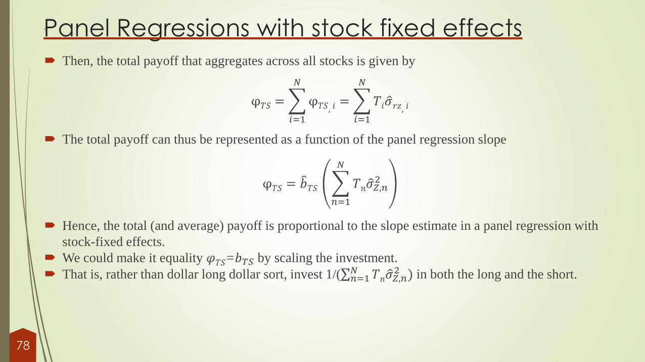
Then, the total payoff that aggregates across all stocks is given by

φ𝑇𝑆 =

𝑖=1

𝑁

φ𝑇𝑆, 𝑖=

𝑖=1

𝑁

𝑇𝑖 ො𝜎𝑟𝑧, 𝑖

The total payoff can thus be represented as a function of the panel regression slope

φ𝑇𝑆 = 𝑏𝑇𝑆

𝑛=1

𝑁

𝑇𝑛 ො𝜎𝑍,𝑛2

Hence, the total (and average) payoff is proportional to the slope estimate in a panel regression with

stock-fixed effects.

We could make it equality 𝜑𝑇𝑆=𝑏𝑇𝑆 by scaling the investment.

That is, rather than dollar long dollar sort, invest 1/(σ𝑛=1𝑁 𝑇𝑛 ො𝜎𝑍,𝑛

2 ) in both the long and the short.

78

Panel Regressions with month fixed effectss

Consider now a panel regression with month-fixed effects

𝑟𝑖𝑡+1 = 𝑎𝑡 + 𝑏𝐶𝑆𝑧𝑖𝑡 + 𝜈𝑖𝑡+1

We use the CS subscript to reflect the notion that month fixed effects correspond to a cross-sectional analysis.

Accounting for month fixed-effects reflects only cross-section variation in the predictive characteristic.

The slope can be estimated through a no-intercept panel regression of future stock return on the demeaned characteristic,

where demeaning is along the cross-section dimension.

The slope of such demeaned regression is readily estimated as

𝑏𝐶𝑆 =σ𝑡=1𝑇 𝑁𝑡 ො𝜎𝑧𝑟, 𝑡σ𝑡=1𝑇 𝑁𝑡 ො𝜎𝑧,𝑡

2

where ො𝜎z,t𝟐 is the cross-sectional variance of the characteristic in month t and ො𝜎𝑧𝑟, 𝑖 is the cross-sectional covariance `

between 𝑟𝑖𝑡+1and zit .

To understand the properties of the slope estimate and its significance, we can express the slope as

𝑏𝐶𝑆 = 𝑏𝐶𝑆 +σ𝑖σ𝑡 𝑧𝑖𝑡 − ҧ𝑧𝑡 휀𝑖𝑡+1

σ𝑡=1𝑇 𝑁𝑡 ො𝜎𝑧,𝑡

2

where ҧ𝑧𝑡 is the time t cross-sectional mean of the predictive characteristic.

79

Panel Regressions with month fixed effects

The slope can be estimated through 𝑏𝐶𝑆 = σ𝑡=1𝑇 𝑤𝑡

𝑏𝑡 where 𝑤𝑡 =𝑁𝑡ෝ𝜎𝑍,𝑡2

σ𝑠=1𝑇 𝑁

𝑠ෝ𝜎𝑍,𝑠2

.

Thus, the slope is a value weighted average of slopes from monthly cross-section regressions:

𝑟𝑖𝑡+1 = 𝑎𝑡 + 𝑏𝑡𝑧𝑖𝑡 + 𝜂𝑖𝑡+1

Larger weights are placed on cross-sectional estimates from periods with more stocks and periods in

which the independent variable exhibits more cross-sectional variation.

Notice that the same slope obtains also through regressing demeaned return on demeaned characteristic

(no month fixed effects), where demeaning is along the cross-section direction.

With stock-fixed effects the weights depend on the number of time-series observations per stock, while

with month fixed-effects, the weights depend on the number of stocks per month.

Also, with stock-fixed effects the weights depend on the time-series variation of the independent variable,

while with month fixed-effects, they depend on the cross-sectional variation.

80

Cross Section based investment strategies

Let us now consider a long-short trading strategy from a cross-sectional perspective:

Long A: zit in stock i at month t

Short B: ҧ𝑧𝑡 in stock i at month t

where ҧ𝑧𝑡 is the time t cross-sectional mean of zit

ҧ𝑧𝑡 =1

𝑁𝑡

𝑖=1

𝑁𝑡

𝑧𝑖𝑡

The total payoff for this long-short strategy is

φ 𝐶𝑆, 𝑡=

𝑖=1

𝑁

𝑧𝑖𝑡 − ҧ𝑧𝑡 𝑟𝑖𝑡+1 = 𝑁𝑡 ො𝜎𝑟𝑧, 𝑡

where ො𝜎𝑟𝑧, 𝑡 is the estimate of month t cross-sectional covariance between 𝑟𝑖𝑡+1and zit .

81

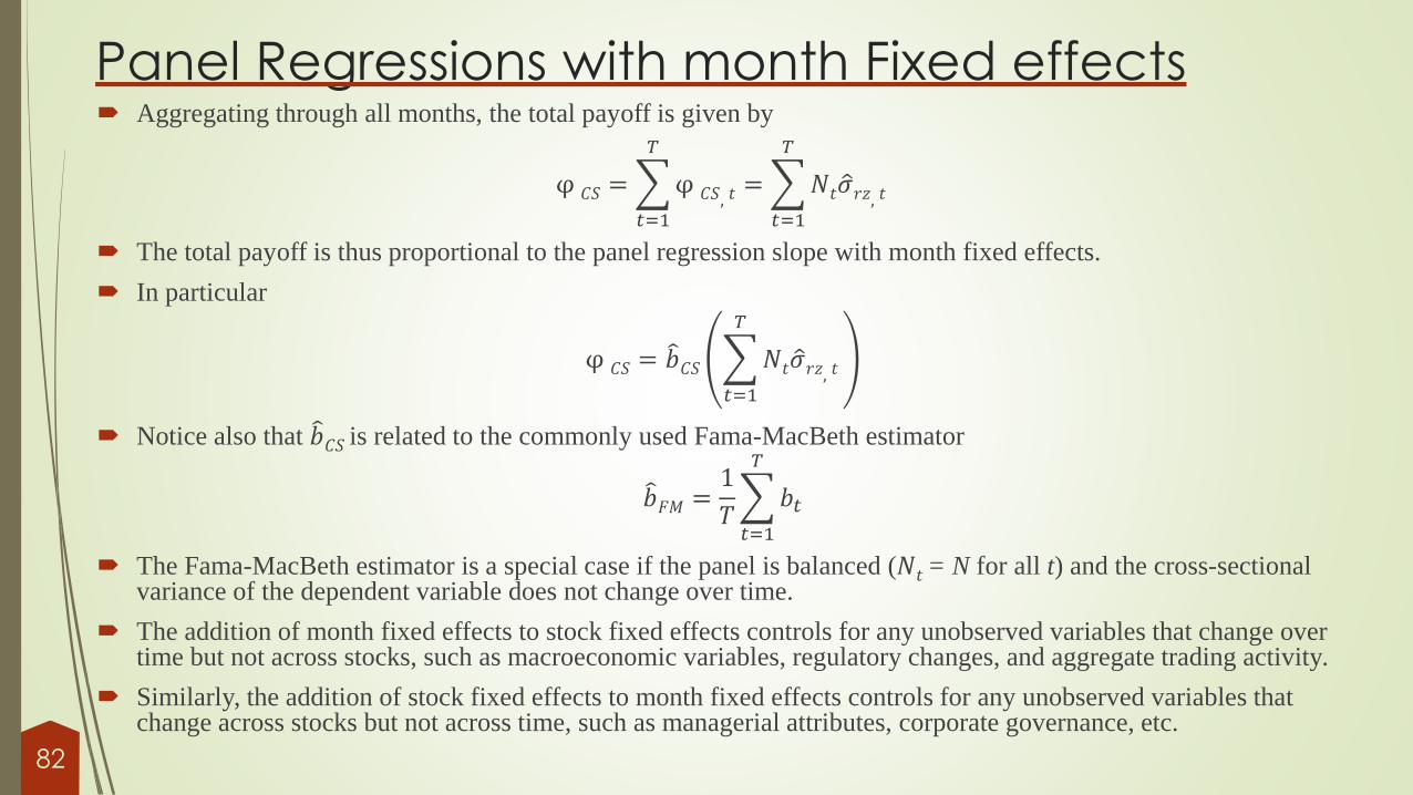
Panel Regressions with month Fixed effects Aggregating through all months, the total payoff is given by

φ 𝐶𝑆 =

𝑡=1

𝑇

φ 𝐶𝑆, 𝑡=

𝑡=1

𝑇

𝑁𝑡 ො𝜎𝑟𝑧, 𝑡

The total payoff is thus proportional to the panel regression slope with month fixed effects.

In particular

φ 𝐶𝑆 = 𝑏𝐶𝑆

𝑡=1

𝑇

𝑁𝑡 ො𝜎𝑟𝑧, 𝑡

Notice also that 𝑏𝐶𝑆 is related to the commonly used Fama-MacBeth estimator

𝑏𝐹𝑀 =1

𝑇

𝑡=1

𝑇

𝑏𝑡

The Fama-MacBeth estimator is a special case if the panel is balanced (𝑁𝑡 = N for all t) and the cross-sectional variance of the dependent variable does not change over time.

The addition of month fixed effects to stock fixed effects controls for any unobserved variables that change over time but not across stocks, such as macroeconomic variables, regulatory changes, and aggregate trading activity.

Similarly, the addition of stock fixed effects to month fixed effects controls for any unobserved variables that change across stocks but not across time, such as managerial attributes, corporate governance, etc.

82

Unconditional Covariance between 𝑟𝑖𝑡+1and 𝑧𝑖𝑡 While Pastor, Stambaugh, and Taylor (2017) have focused on conditional covariation between future return and

current value of characteristic, it is also intriguing to understand the sources of unconditional covariation.

The unconditional covariance between future stock return and the current value of firm characteristic is not conditioned on either stock fixed effects or time fixed effects.

We show below that the unconditional covariance can also be expressed as a function of payoffs attributable to time-series and cross-sectional strategies.

In particular, let ҧ𝑧= 1

σ𝑖 𝑇𝑖σ𝑖σ𝑡 𝑧𝑖𝑡 and ҧ𝑟=

1

σ𝑖 𝑇𝑖σ𝑖σ𝑡 𝑟𝑖𝑡+1.

These quantities are the grand means (across months and stocks) of the characteristic and return.

The estimated unconditional covariance is then given by

𝐶𝑂𝑉 =

𝑖

𝑡

𝑧𝑖𝑡 − ҧ𝑧 𝑟𝑖𝑡+1 − ҧ𝑟

=

𝑖

𝑡

𝑧𝑖𝑡 − ҧ𝑧 𝑟𝑖𝑡+1

83

Unconditional Covariance between 𝑟𝑖𝑡+1and 𝑧𝑖𝑡 As an intermediate stage, let us decompose the payoffs to the time-series and cross-sectional

strategies as follows

φ𝑇𝑆 =

𝑖

𝑡

𝑧𝑖𝑡 − ҧ𝑧𝑖 𝑟𝑖𝑡+1 =

𝑖

𝑡

ҧ𝑧𝑡 − ҧ𝑧 𝑟𝑖𝑡+1

A

+

𝑖

𝑡

𝑧𝑖𝑡 − ҧ𝑧𝑡 − ҧ𝑧𝑖 − ҧ𝑧 𝑟𝑖𝑡+1

𝐵

φ 𝐶𝑆 =

𝑖

𝑡

𝑧𝑖𝑡 − ഥ𝑧𝑡 𝑟𝑖𝑡+1 =

𝑖

𝑡

ҧ𝑧𝑖 − ҧ𝑧 𝑟𝑖𝑡+1

𝐶

+

𝑖

𝑡

𝑧𝑖𝑡 − ҧ𝑧𝑡 − ҧ𝑧𝑖 − ҧ𝑧 𝑟𝑖𝑡+1

𝐵

Notice that the payoffs for the time-series and cross-sectional strategies do share a common

component (B) reflecting through-time-across-stock payoff.

Notice also that both strategies do have unique components A and C reflecting purely through-

time and across-stock payoffs, respectively.

Let us now decompose the difference 𝑧𝑖𝑡 − ҧ𝑧 such that

𝑧𝑖𝑡 − ҧ𝑧 = ҧ𝑧𝑡 − ҧ𝑧 + 𝑧𝑖𝑡 − ҧ𝑧𝑡 − ҧ𝑧𝑖 − ҧ𝑧 + ҧ𝑧𝑖 − ҧ𝑧84

Unconditional Covariance between 𝑟𝑖𝑡+1and 𝑧𝑖𝑡 Thus, the unconditional covariance between future stock return and the current value of predictive characteristic

is given by

𝐶𝑂𝑉 𝑟𝑖𝑡+1 , 𝑧𝑖𝑡 = 𝐴 + 𝐵 + 𝐶

In words, the estimated unconditional covariance is equal to the sum of the unique time-series payoff (A), the unique cross-sectional payoff (C), and the common component (B).

Now, let 𝛾 denote the slope in the unconditional (no fixed effects) panel regression.

The slope is estimated as

ො𝛾 =σ𝑖 σ𝑡 𝑧𝑖𝑡− ҧ𝑧 𝑟𝑖𝑡+1− ҧ𝑟

σ𝑖 σ𝑡 𝑧𝑖𝑡− ҧ𝑧2

The slope can then be decomposed into its three components reflecting the contribution of A, B, and C in explaining the total variation (through time and across stocks) in return:

ො𝛾 = ො𝛾A+ ො𝛾B+ො𝛾C.

For instance,

ො𝛾𝐴 =𝐴

σ𝑖 σ𝑡 𝑧𝑖𝑡− ҧ𝑧2

Avramov and Xu (2019) implement such slope decomposition in the context of predicting future currency return by the foreign interest rate for various economies.

85

Unconditional Covariance between 𝑟𝑖𝑡+1and 𝑧𝑖𝑡 To understand the quantity ො𝛾𝐴, consider the regression of return rit+1 on ҧ𝑧t.

The estimated slope in that regression is denoted by መ𝛿𝐴.

Then, it follows that

ො𝛾𝐴 = መ𝛿𝐴𝑉𝐴𝑅 ( ҧ𝑧

𝑡)

𝑉𝐴𝑅 (𝑧𝑖𝑡)

Similarly, consider the regression of return rit+1 on ҧ𝑧i.

The estimated slope in this regression is denoted by መ𝛿𝑐.

Then, it follows that

ො𝛾𝐶 = መ𝛿𝐶𝑉𝐴𝑅 ( ҧ𝑧

𝑡)

𝑉𝐴𝑅 (𝑧𝑖𝑡)

Notice also that መ𝛿𝐴 =𝐴

𝑉𝐴𝑅 ( ҧ𝑧𝑡)

and መ𝛿𝐶 =𝐶

𝑉𝐴𝑅 ( ҧ𝑧𝑖).

Significance of ො𝛾 is easily inferred from the unconditional regression while signifnace of ො𝛾A, ො𝛾B, or ො𝛾C or

significance of ratios such as A/C can be assessed through Jackknife or Bootstrap (see Avramov and Xu (2019)).

The ratio A/C reflects the strength of time-series versus cross-sectional strategies.

86

Multiple Panel regressions with fixed effects Thus far, we have studied univariate panel regressions.

Consider now a multiple panel regression with stock fixed effects

𝑟𝑖𝑡+1 = 𝑎𝑖 + 𝑏𝑇𝑆′𝑧𝑖𝑡 + 휀𝑖𝑡+1

𝑧𝑖𝑡 is an M-vector of characteristics for firm i at month t and 𝑏𝑇𝑆 is an M-vector of slope coefficients.

We thus have to estimate N intercepts (a1,a2,…,aN) along with M slopes, altogether (N+M ) parameters.

OLS coefficients are given byො𝑎1ො𝑎2⋮ො𝑎𝑁𝑏𝑇𝑆

= (𝑋′𝑋) −1𝑋′𝑅

Let ෨𝑇 = σ𝑖=1𝑁 𝑇𝑖, then R is a ෨𝑇-vector, 𝑅′ = 𝑟′1, 𝑟

′2, … , 𝑟′𝑁 , with ri being a Ti-vector of returns for firm i.

87

Multiple Panel regressions with fixed effects In addition, X is a ෨𝑇 × (𝑀 + 𝑁) matrix:

𝑋 =

𝜄10⋮

0𝜄2⋮

0 0

⋯⋯⋱⋯

00⋮𝜄𝑁

𝑧1𝑧2⋮𝑧𝑁

Then, it can be shown that

𝑏𝑇𝑆 =

𝑖=1

𝑁

𝑤𝑖𝑏𝑖

where 𝑤𝑖 = 𝑇𝑖 σ𝑠=1𝑁 𝑇𝑠 Σzs

−1 Σzi , Σzi is the time-series covariance matrix of firm i characteristics, and 𝑏𝑖 is an M-vector

of slope estimates from individual predictive regressions of future returns on current values of firm characteristics.

As in the univariate case, the slope is a value weighted average of firm-level slopes but now weights are formulated through an 𝑀 ×𝑀 matrix.

The slope can also be represented as

𝑏𝑇𝑆 =

𝑠=1

𝑁

𝑇𝑠 Σzs

−1

𝑖=1

𝑁

𝑇𝑖Σzri , where Σzri is a covariance vector between future return and 𝑀 characteristics.

88

Multiple Panel regressions with fixed effects Similarly, consider a multiple regression with month fixed-effects:

𝑟𝑖𝑡+1 = 𝑎𝑡 + 𝑏𝐶𝑆′𝑧𝑖𝑡 + 휀𝑖𝑡+1

We estimate T intercepts and M slops coefficients, altogether T+M parameters.

The slope estimate is given by:

𝑏𝐶𝑆 =

𝑡=1

𝑇

𝑤𝑡𝑏𝑡

where 𝑏𝑡 is an M-vector of slopes estimated from monthly cross section regressions,

𝑤𝑡 =Nt σ𝑠=1𝑇 𝑁𝑆

𝛴zS

−1 𝛴zt , and 𝛴zt is the month-t cross-sectional covariance matrix of firm

characteristics.

89

Panel regressions with Common Factors Let us now extend the panel regression setup to account for common factors.

To keep it simple, let us consider a single factor model.

Then, the panel regression is formulates as

𝑟𝑖𝑡+1 = 𝑎𝑖 + 𝑟𝑓𝑡 + 𝛽𝑖ft+1 + 𝛾 zit + 휀𝑖𝑡+1

𝑟𝑓𝑡 is the risk-free rate for period t+1, observed at time t.

Clearly, 𝑟𝑓𝑡 and ft+1 vary only through time but not across stocks.

In the time-invariant beta setup, beta varies only across stocks.

Essentially, we ask what does the 𝛽𝑖ft+1 component capture?

It can capture cross-sectional predictability if 𝛽𝑖 is correlated, in the cross section, with the characteristic.

It can also capture time-series predictability if, for at least one stock, ft+1 is correlated, in the time series, with zit .

We formalize these concepts below.

90

Panel regressions with Common Factors Let us define risk adjusted excess return as ǁ𝑟𝑖t+1 = 𝑟𝑖𝑡+1 − 𝑟𝑓𝑡 − 𝛽𝑖ft+1 .

The corresponding payoffs to the time-series and cross-sectional strategies are given by

φ𝑇𝑆 =

𝑖

𝑡

𝑧𝑖𝑡 − ҧ𝑧𝑖 ǁ𝑟𝑖𝑡+1 = ෩𝐴 + ෨𝐵

φ𝐶𝑆 =

𝑖

𝑡

𝑧𝑖𝑡 − ҧ𝑧𝑡 ǁ𝑟𝑖𝑡+1 = ሚ𝐶 + ෨𝐵

where ෩𝐴 , ෨𝐵, and ሚ𝐶 are similar to A, B ,and C except that ǁ𝑟𝑖𝑡+1is replacing 𝑟𝑖𝑡+1.

Then, it can be shown that

෩𝐴 = 𝐴 −

𝑖

𝑡

𝑧𝑖𝑡 − ҧ𝑧𝑖 𝛽𝑖ft+1

෩𝐴 = 𝐴 −

𝑖

𝛽𝑖

𝑡

𝑧𝑖𝑡 − ҧ𝑧𝑖 ft+1

෩𝐴 = 𝐴 −

𝑖

𝛽𝑖 Ti ො𝜎𝑧𝑓, 𝑖

where ො𝜎𝑧𝑓, 𝑖 is the time-series covariance between ft+1 and 𝑧𝑖𝑡 and Ti is the number of time-series observations per stock i.

91

Panel regressions with Common Factors The last equation formalizes the notion that including common factors can capture time-series

predictability by firm characteristics as long as the factor is correlated with the lagged characteristic

for at least one stock.

Clearly, if ො𝜎𝑧𝑓, 𝑖 is equal to zero for each of the stocks then asset pricing factors do not explain any

time-series predictability.

From a cross-sectional perspective, it follows that

ሚ𝐶 = 𝐶 − σ𝑖σ𝑡 ҧ𝑧𝑖𝑡 − ҧ𝑧𝑡 𝛽𝑖ft+1

= 𝐶 − σ𝑡 ft+1σ𝑖 ҧ𝑧𝑖𝑡 − ҧ𝑧𝑡 𝛽𝑖

= 𝐶 − σ𝑡=1𝑇 Ntft+1 ො𝜎𝛽𝑧, 𝑡

where ො𝜎𝛽𝑧, 𝑡 is the cross-section covariance between 𝛽𝑖 and zit while 𝑁𝑡 is the number of stocks at

month t.

Asset pricing factors could explain cross-sectional predictability as long as factor loadings are

correlated with firm characteristics, for at least one period.

92

Machine learning Methods in asset

pricing

* I thank Lior Metzker for his help in writing several paragraphs in this section

93

Machine learning Methods in asset pricing

Machine learning typically prescribes a vast collection of high-dimensional models

attempting to predict quantities of interest while imposing regularization methods.

Below, I provide general descriptions of machine learning methods and discuss how such

methods have successfully been implemented in asset pricing.

For perspective, it is well known that the ordinary least squares (OLS) estimator is the

best linear unbiased estimator (BLUE) of the regression coefficients.

“Best" means the lowest variance estimator among all other unbiased linear estimators.

Notice that the regression errors do not have to be normal, nor do they have to be

independent and identically distributed – but they have to be uncorrelated with mean

zero and homoskedastic with finite variance.

In the presence of either heteroskedasticity or autocorrelation, OLS is no longer BLUE.

94

Shortcomings of OLS

With heteroskedasticity, we can still use the OLS estimators by finding

heteroskedasticity-robust estimators of the variance, or we can devise an efficient

estimator by re-weighting the data appropriately to incorporate heteroskedasticity.

Similarly, with autocorrelation, we can find an autocorrelation-robust estimator of the

variance. Alternatively, we can devise an efficient estimator by re-weighting the data

appropriately to account for autocorrelation.

Notice also that the requirement for an unbiased estimator is crucial since biased

estimators do exist.

This is where shrinkage methods come to play: the variance of the OLS estimator can be

too high as the OLS coefficients are unregulated.

If judged by Mean Squared Error (MSE), alternative biased estimators could be more

attractive if they produce substantially smaller variance.

In particular, let 𝛽 denotes the true coefficient and let መ𝛽 = (𝑋′𝑋)−1𝑋′𝑌, where 𝑋 is a 𝑇×𝑀 matrix of explanatory variables and 𝑌 is a 𝑇 × 1 vector of the dependent variable.

95

Shortcomings of OLS Then

MSE መ𝛽 = 𝐸 መ𝛽 − 𝛽′ መ𝛽 − 𝛽

= 𝐸 tr መ𝛽 − 𝛽′ መ𝛽 − 𝛽

= 𝐸 tr መ𝛽 − 𝛽 መ𝛽 − 𝛽′

= tr 𝐸 መ𝛽 − 𝛽 መ𝛽 − 𝛽′

= 𝜎2tr[ 𝑋′𝑋 −1]

When predictors are highly correlated the expression tr 𝑋′𝑋 −1 can explode.

Moreover, in the presence of many predictors, OLS delivers nonzero estimates for all coefficients – thus it is difficult to implement variable selection when the true data generating process has a sparse representation.

The OLS solution is not unique if the design if X is not full rank.

The OLS does not account for potential non linearities and interactions between predictors.

In sum, OLS is restrictive, often provide poor predictions, may be subject to over-fitting, does not penalize for model complexity, and could be difficult to interpret.

From a Bayesian perspective, one can think of introducing priors on regression coefficients to make the coefficients smaller in magnitude or even zero them out altogether.

From a classical (non Bayesian) perspective, shrinkage methods are about penalizing complexity.

96

Economic restrictions on OLS While the next pages discuss shrinkage methods, here are two ways to potentially improve OLS estimates.

Base case: the pooled OLS estimator corresponds to a panel (balanced) regression of future returns on firm attributes, where T and N represent again the time-series and cross-section dimensions.

The objective is formulated as

ℒ 𝜃 =1

𝑁𝑇

𝑖=1

𝑁

𝑡=1

𝑇

𝑟𝑖,𝑡+1 − 𝑓 𝑐𝑖,𝑡; 𝜃2

where f 𝑐𝑖,𝑡; 𝜃 = 𝑐𝑖,𝑡′ 𝜃, 𝑟𝑖,𝑡+1 is stock return at time t+1 per firm i, and 𝑐𝑖,𝑡 is an M-vector of firm i attributes realized at time t.

Predictive performance could be improved using an alternative optimization where stocks are weighted differently based on market size, volatility, credit quality, etc.:

ℒ 𝜃 =1

𝑁𝑇

𝑖=1

𝑁

𝑡=1

𝑇

𝑤𝑖,𝑡 𝑟𝑖,𝑡+1 − 𝑓 𝑐𝑖,𝑡; 𝜃2

An alternative economic based optimization takes account of the heavy tail displaed by stocks and the potential harmul effects of outliers. Then the objective is formulated such that squared (absolute) loss is applied to small (large) errors:

ℒ 𝜃 =1

𝑁𝑇

𝑖=1

𝑁

𝑡=1

𝑇

𝐻 𝑟𝑖,𝑡+1 − 𝑓 𝑐𝑖,𝑡; 𝜃 , 𝜉

where 𝜉 is a tuning parameter and

𝐻 𝑥, 𝜉 =𝑥2, if 𝑥 ≤ 𝜉

2𝜉 𝑥 − 𝜉2, if 𝑥 > 𝜉97

Ridge Regression There are various shrinkage methods.

We start with Ridge.

Hoerl and Kennard (1970a, 1970b) introduce the Ridge regression

min (𝑌 − 𝑋𝛽)′(𝑌 − 𝑋𝛽) s. t. σ𝑗=1𝑀 𝛽𝑗

2 ≤ 𝑐

The minimization can be rewritten as

ℒ 𝛽 = 𝑌 − 𝑋𝛽 ′ 𝑌 − 𝑋𝛽 + 𝜆(𝛽′𝛽)

We get መ𝛽ridge = (𝑋′𝑋 + 𝜆𝐼𝑀)

−1𝑋′𝑌

Notice that including 𝜆 makes the problem non-singular even when 𝑋′𝑋 is non invertible.

𝜆 is an hyper-parameter that controls for the amount of regularization.

98

Ridge Regression

As 𝜆 → 0, the OLS estimator obtains.

As 𝜆 → ∞, we have መ𝛽ridge = 0, or intercept-only model.

Ridge regressions do not have a sparse representation, so using model selection criteria to

pick 𝜆 does not seem to be feasible.

Instead, validation methods are often employed.

The notion of validation is to split the sample into three pieces: training, validation, and test.

The training sample considers various values for 𝜆 each of which delivers a prediction. The

validation sample is choosing the 𝜆 that provides the best prediction. Hence, both training

and validation samples are used to pick 𝜆. Then the experiment is assessed through out-of-

sample predictions.

As shown below, from a Bayesian perspective, the parameter 𝜆 denotes the prior precision of

beliefs that regression slope coefficients are all equal to zero.

From a non Bayesian perspective, the ridge estimator is essentially biased:

𝐸 መ𝛽ridge = [𝐼𝑀 + 𝜆 𝑋′𝑋 −1]𝛽 ≠ 𝛽99

Interpretations of the Ridge RegressionInterpretation #1: Data Augmentation

The ridge-minimization problem can be formulated as

𝑡=1

𝑇

(𝑦𝑡 − 𝑥𝑡′𝛽)2 +

𝑗=1

𝑀

0 − 𝜆𝛽𝑗2

Thus, the ridge-estimator is the usual OLS estimator where the data is transformed such that

𝑋𝜆 =𝑋

𝜆𝐼𝑀, 𝑌𝜆 =

𝑌0𝑀

Then,መ𝛽ridge = 𝑋𝜆

′𝑋𝜆−1𝑋𝜆

′𝑌𝜆

Interpretation #2: Eigen-values and Eigen-vectors

By the singular value decomposition, we can express 𝑋 as

𝑋𝑇×𝑀 = 𝑈𝑇×𝑀Λ𝑀×𝑀0.5 𝑉𝑀×𝑀

′

where 𝑈 = [𝑈1, … , 𝑈𝑀] is any 𝑇 ×𝑀 orthogonal matrix, Λ0.5 =𝜆10.5 ⋯ 0⋮ ⋱ ⋮0 ⋯ 𝜆𝑀

0.5is an 𝑀 ×𝑀 matrix s. t.

100

Interpretations of the Ridge Regression 𝜆1 ≥ 𝜆2 ≥ ⋯ ≥ 𝜆𝑀, and 𝑉 = 𝑉1, 𝑉2, … , 𝑉𝑀 is an 𝑀 ×𝑀 orthogonal matrix.

As 𝑋′𝑋 = 𝑉Λ𝑉′, the matrix V denotes the eigenvectors of 𝑋′𝑋 and (𝜆1, … , 𝜆𝑀) are the corresponding eigenvalues

How is the predicted value of Y related to eigen vectors?

To answer, we would like first to find the eigenvectors and eigenvalues of the matrix 𝑍

𝑍 = 𝑋′𝑋 + 𝜆𝐼𝑀

We know that for every j=1,2…,M, the following holds by definition

𝑋′𝑋 𝑉𝑗 = 𝜆𝑗𝑉𝑗

Thus

𝑋′𝑋 + 𝜆𝐼𝑀 𝑉𝑗 = 𝑋′𝑋 𝑉𝑗 + 𝜆𝑉𝑗= 𝜆𝑗𝑉𝑗 + 𝜆𝑉𝑗 = 𝜆𝑗 + 𝜆 𝑉𝑗

Telling you that 𝑉 still denotes the eigenvectors of 𝑍 and 𝜆𝑗 + 𝜆 is the 𝑗-th eigenvalue.

Notice now that if 𝐴 = 𝑉Λ𝑉′ then 𝐴𝑁 = 𝑉Λ𝑁𝑉′.

Same eigenvectors while eigenvalues are raised to the power of 𝑁. 101

Interpretations of the Ridge Regression

Then, the inverse of the matrix Z is given by

𝑍−1 = 𝑉 𝑑𝑖𝑎𝑔1

𝜆1 + 𝜆,

1

𝜆2 + 𝜆,… ,

1

𝜆𝑀 + 𝜆𝑉′

Andመ𝛽ridge = 𝑍−1𝑋′𝑌 = 𝑋′𝑋 + 𝜆𝐼𝑀

−1𝑋′𝑌

= 𝑉 𝑑𝑖𝑎𝑔𝜆10.5

𝜆1 + 𝜆,𝜆20.5

𝜆2 + 𝜆,… ,

𝜆𝑀0.5

𝜆𝑀 + 𝜆𝑈′𝑌

And the fitted value is

𝑌ridge = 𝑋 መ𝛽ridge = 𝑗=1

𝑀

(𝑈𝑗𝜆𝑗

𝜆𝑗 + 𝜆𝑈𝑗′) 𝑌

Hence, ridge regression projects 𝑌 onto components with large 𝜆𝑗.

Or, ridge regression shrinks the coefficients of low variance components.

102

Informative Bayes PriorInterpretation #3: Informative Bayes Prior

Suppose that the prior on 𝛽 is of the form:

𝛽~𝑁 0,1

𝜆𝐼𝑀

Then, the posterior mean of 𝛽 is:

(𝑋′𝑋 + 𝜆𝐼𝑀)−1𝑋′𝑌

While we discuss Bayesian approaches later in the notes, consider the family of priors for mean return 𝜇:

𝜇~𝑁 0,𝜎2

𝑠2𝑉𝜂

where 𝑠2 = 𝑡𝑟𝑎𝑐𝑒 𝑉 which is also the sum of the eigenvalues of 𝑉, or 𝑠2 = σ𝑗=1𝑁 𝜆𝑗.

To see why, notice that 𝑡𝑟𝑎𝑐𝑒 𝑉 = 𝑡𝑟𝑎𝑐𝑒 𝑄𝛬𝑄′ = 𝑡𝑟𝑎𝑐𝑒 𝛬𝑄′𝑄 = 𝑡𝑟𝑎𝑐𝑒 𝛬 = σ𝑗=1𝑁 𝜆𝑗

𝜎2 is a constant controlling for the degree of confidence in the prior.

The case 𝜂 = 1 gives the asset pricing prior of Pastor (2000) and Pastor and Stambaugh (2000).

The case 𝜂 = 2 gives the prior motivated by Kozak, Nagel, and Santosh (2017b).

The Pastor-Stambaugh prior seems more flexible since factors are pre-specified and are not ordered per their importance.

103

Informative Bayes Prior

Let us again make the projection of the original space of returns into the space of

principal components:

𝑀𝑡 = 1 − 𝜇′𝑉−1 𝑟𝑡 − 𝜇= 1 − 𝜇′𝑄Λ−1𝑄′ 𝑟𝑡 − 𝜇

= 1 − 𝜇𝑄′ Λ−1 𝑄𝑡 − 𝜇𝑄

= 1 − 𝑏𝑄′ 𝑄𝑡 − 𝜇𝑄

As 𝜇~𝑁 0,𝜎2

𝑠2𝑉𝜂 it follows that 𝜇𝑄 = 𝑄′𝜇 has the prior distribution

𝜇𝑄 = 𝑄′𝜇 ~ 𝑁 0,𝜎2

𝑠2𝑄′𝑉𝜂𝑄

~𝑁 0,𝜎2

𝑠2𝑄′𝑄Λ𝜂𝑄′𝑄

~ 𝑁 0,𝜎2

𝑠2Λ𝜂

104

Informative Bayes Prior As 𝑏𝑄 = Λ−1𝜇𝑄 its prior distribution is formulated as (Λ is assumed known):

𝑏𝑄 = Λ−1𝜇𝑄 ~ 𝑁 0,𝜎2

𝑠2Λ𝜂−2

Notice that for 𝜂 < 2 the variance of the 𝑏𝑄 coefficients associated with the smallest eigenvalues explodes.

For 𝜂 = 2, the pricing kernel coefficients 𝑏 = 𝑉−1𝜇 have the prior distribution

𝑏~𝑁 0,𝜎2

𝑠2𝐼𝑁

Picking 𝜂 = 2 makes the prior of 𝑏 independent of 𝑉.

Further, the likelihood of 𝑏 is given by

𝑏~𝑁 𝑉−1 Ƹ𝜇,1

𝑇𝑉−1

where Ƹ𝜇 is the sample mean return.

Then, the posterior mean of 𝑏 is given by 𝐸 𝑏 = 𝑉 + 𝜆𝐼𝑁−1 Ƹ𝜇 where 𝜆 =

𝑠2

𝑇𝜎2.

The posterior variance is 𝑣𝑎𝑟 𝑏 =1

𝑇𝑉 + 𝜆𝐼𝑁

−1.

Similar to the ridge regression with a tuning parameter 𝜆.

105

Informative Bayes Prior The prior expected value of the squared SR is given by (V is assumed known):

𝐸 𝑆𝑅2 = 𝐸 𝜇′𝑉−1𝜇= 𝐸 𝜇′𝑄Λ−1𝑄′𝜇

= 𝐸 𝜇𝑄′ Λ−1𝜇𝑄

= 𝐸 𝑡𝑟𝑎𝑐𝑒 𝜇𝑄′ 𝛬−1𝜇𝑄

= 𝑡𝑟𝑎𝑐𝑒 𝛬−1𝐸 𝜇𝑄𝜇𝑄′

=𝜎2

𝑠2𝑡𝑟𝑎𝑐𝑒 𝛬𝜂−1

The Pastor-Stambaugh prior (𝜂 = 1 ) tells you that

𝐸 𝑆𝑅2 =𝜎2

𝑠2𝑡𝑟𝑎𝑐𝑒 𝐼𝑁 = 𝑁

𝜎2

𝑠2

That is, each principal component portfolio has the same expected contribution to the Sharpe ratio.

If 𝜂 = 2, then

𝐸 𝑆𝑅2 =

𝑗=1

𝑁𝜎2

𝑠2𝜆𝑗 = 𝜎2

Then, the expected contribution of each PC is proportional to its eigenvalue.

This reinforces the notion that only the first few principal components could explain the cross section variation in expected returns.

106

Lasso

We now consider various Lasso (least absolute shrinkage and selection operator) models.

Tibshirani (1996) was the first to introduce Lasso.

Lasso simultaneously performs variable selection and coefficient estimation via shrinkage.

While the ridge regression implements an 𝑙2-penalty, Lasso is an 𝑙1-optimization:

min (𝑌 − 𝑋𝛽)′(𝑌 − 𝑋𝛽) s. t.

𝑗=1

𝑀

|𝛽𝑗| ≤ 𝑐

The 𝑙1 penalization approach is called basis pursuit in signal processing.

We have again a non-negative tuning parameter 𝜆 that controls the amount of regularization:

ℒ 𝛽 = 𝑌 − 𝑋𝛽 ′ 𝑌 − 𝑋𝛽 + 𝜆𝑗=1

𝑀

|𝛽𝑗|

Both Ridge and Lasso have solutions even when 𝑋′𝑋 may not be of full rank (e.g., when there are more

explanatory variables than time-series observations) or ill conditioned.

107

Lasso

Unlike Ridge, the Lasso coefficients cannot be expressed in closed form.

However, Lasso can provide with a set of sparse solutions.

This improves the interpretability of regression models.

Large enough 𝜆, or small enough 𝑐, will set some coefficients exactly to zero.

To understand why, notice that LASSO can be casted as having a Laplace prior 𝛽

𝑃 𝛽 𝜆 ∝𝜆

2𝜎exp −

𝜆 𝛽

𝜎

In particular, Lasso obtains by combining Laplace prior and normal likelihood.

Like the normal distribution, Laplace is symmetric.

Unlike the normal distribution, Laplace has a spike at zero (first derivative is discontinuous)

and it concentrates its probability mass closer to zero than does the normal distribution.

This could explain why Lasso (Laplace prior) sets some coefficients to zero, while Ridge

(normal prior) does not.

108

Lasso

Bayesian information criterion (BIC) is often used to pick 𝜆.

BIC (like other model selection criteria) is composed of two components: the sum of squared

regression errors and a penalty factor that gets larger as the number of retained characteristics

increases.

𝐵𝐼𝐶 = 𝑇 × 𝑙𝑜𝑔𝑅𝑆𝑆

𝑇+ 𝑘 × 𝑙𝑜𝑔 𝑇 , where 𝑘 is the number of retained characteristics.

Notice that different values of lambda affect the optimization in a way that a different set of

characteristics is selected.

You choose 𝜆 as follows: initiate a range of values, compute BIC for each value, and pick the

one that minimizes BIC.

The next page provides steps for assessing the maximum value of 𝜆 in formulating the range.

109

Lasso

For convenience, let us formulate again the objective function

ℒ 𝛽 = 𝑌 − 𝑋𝛽 ′ 𝑌 − 𝑋𝛽 + 𝜆σ𝑗=1𝑀 |𝛽𝑗|

If a change of 𝛽 does not decrease the objective function ℒ 𝛽 , then it is a local minimum.

An infinitesimal change in 𝛽𝑗, 𝜕𝛽𝑗 would change the objective function ℒ 𝛽 as follows

The penalty term changes by 𝜆𝑠𝑖𝑔𝑛 𝛽𝑗 𝜕𝛽𝑗

The squared error term changes by 𝜕𝑅𝑆𝑆 = 2𝑌′𝑋𝑗 + 2𝛽𝑗 𝜕𝛽𝑗 , where 𝑋𝑗 is the 𝑗’s row of the

matrix 𝑋.

If 𝛽 = 0 then 𝜕𝑅𝑆𝑆 = 2𝑌′𝑋𝑗 𝜕𝛽𝑗

For the objective function to decrease, the change in the RSS should be greater than the change in

penalty:

2𝑌′𝑋𝑗 𝜕𝛽𝑗

𝜆𝑠𝑖𝑔𝑛 𝛽𝑗 𝜕𝛽𝑗> 1 , hence 𝜆 < 2𝑌′𝑋𝑗 , or

𝜆 = max𝑗

2𝑌′𝑋𝑗

110

Adaptive Lasso and Bridge regression LASSO forces coefficients to be equally penalized.

One modification is to assign different weights to different coefficients:

ℒ 𝛽 = 𝑌 − 𝑋𝛽 ′ 𝑌 − 𝑋𝛽 + 𝜆σ𝑗=1𝑀 𝑤𝑗|𝛽𝑗|

It can be shown that if the weights are data driven and are chosen in the right way such weighted LASSO can

have the so-called oracle properties even when the LASSO does not. This is the adaptive LASSO.

For instance, 𝑤𝑗 can be chosen such that it is equal to one divided by the absolute value of the corresponding

OLS coefficient raised to the power of 𝛾 > 0. That is, 𝑤𝑗 =1

𝛽𝑗𝛾 for 𝑗 = 1,… ,𝑀.

The adaptive LASSO estimates are given by

ℒ 𝛽 = 𝑌 − 𝑋𝛽 ′ 𝑌 − 𝑋𝛽 + 𝜆σ𝑗=1𝑀 𝑤𝑗|𝛽𝑗|

The adaptive LASSO is a convex optimization problem and thus does not suffer from multiple local minima

Frank and Friedman (1993) introduce the bridge regression, which generalizes for ℓq penalty

ℒ 𝛽 = 𝑌 − 𝑋𝛽 ′ 𝑌 − 𝑋𝛽 + 𝜆σ𝑗=1𝑀 𝛽𝑗

𝑞

Notice that 𝑞 = 0, 1, 2, correspond to OLS, LASSO, and ridge, respectively.

Moreover, the optimization is convex for 𝑞 ≥ 1 and the solution is sparse for 0 ≤ 𝑞 ≤ 1.

111

The Elastic Net The elastic net is yet another regularization and variable selection method.

Zou and Hastie (2005) describe it as stretchable fishing net that retains “all big fish”.

Using simulation, they show that it often outperforms Lasso in terms of prediction

accuracy.

The elastic net encourages a grouping effect, where strongly correlated predictors tend to

be in or out of the model together.

The elastic net is particularly useful when the number of predictors is much bigger than

the number of observations.

The naïve version of the elastic net is formulated through

ℒ 𝛽 = 𝑌 − 𝑋𝛽 ′ 𝑌 − 𝑋𝛽 + 𝜆1𝑗=1

𝑀

|𝛽𝑗| + 𝜆2𝑗=1

𝑀

𝛽𝑗2

Thus, the elastic net combines 𝑙1 and 𝑙2 norm penalties.

It still produces sparse representations.

112

Group Lasso Again, the data consist of 𝑌, a T-vector of the dependent variable, and 𝑋, a 𝑇 ×𝑀 matrix of explanatory

variables.

Suppose that the 𝑀 predictors are divided into 𝐿 groups, with 𝑀𝑙 denoting the number of predictors in group 𝑙.

𝑋𝑙 represents the predictors corresponding to the 𝑙-th group, while 𝛽𝑙 is the corresponding coefficient vector.

Notice, 𝛽=[𝛽1′ , 𝛽2

′ , … , 𝛽𝐿′ ]’.

Assume that both 𝑌 and 𝑋 have been centered.

The group Lasso solves the convex optimization problem.

ℒ 𝛽 = 𝑌 −

𝑙=1

𝐿

𝑋𝑙𝛽𝑙

′

𝑌 −

𝑙=1

𝐿

𝑋𝑙𝛽𝑙 + 𝜆

𝑙=1

𝐿

𝛽𝑙′𝛽𝑙

12

The group Lasso does not yield sparsity within a group.

If a group of parameters is non-zero, they will all be non-zero.

The sparse group Lasso criterion does yield sparsity

ℒ 𝛽 = 𝑌 −

𝑙=1

𝐿

𝑋𝑙𝛽𝑙

′

𝑌 −

𝑙=1

𝐿

𝑋𝑙𝛽𝑙 + 𝜆1

𝑙=1

𝐿

𝛽𝑙′𝛽𝑙

12

+ 𝜆2

𝑗=1

𝑀

𝛽𝑗

113

Non parametric shrinkage Lasso, Adaptive Lasso, Group Lasso, Ridge, Bridge, and Elastic net are all linear or

parametric approaches for shrinkage.

Group Lasso implements the same penalty to predictors belonging to some pre-specified group while different penalty applies to different groups.

Some other parametric approaches (uncovered here) include the smoothed clip absolute deviation (SCAD) penalty of Fang and Li (2001) and Fang and Peng (2004) and the minimum concave penalty of Zhang (2010).

In many application, however, there is little a priori justification for assuming that the effects of covariates take a linear form or belong to other known parametric family.

Huang, Horowitz, and Wei (2010) thus propose to use a nonparametric approach: the adaptive group Lasso for variable selection.

This approach is based on a spline approximation to the nonparametric components.

To achieve model selection consistency, they apply the group Lasso in two steps.

First, they use the group Lasso to obtain an initial estimator and reduce the dimension of the problem.

Second, they use the adaptive group Lasso to select the final set of nonparametric components.

114

In finance, Cochrane (2011) notes that portfolio sorts are the same thing as nonparametric cross section regressions.

Drawing on Huang, Horowitz, and Wei (2010), Freyberger, Neuhier, and Weber (2017) study this equivalence formally.

The cross section of stock returns is modelled as a non-linear function of firm characteristics:

𝑟𝑖𝑡 = 𝑚𝑡 𝐶1,𝑖𝑡−1, … , 𝐶𝑆,𝑖𝑡−1 + 𝜖𝑖𝑡

Notation:

𝑟𝑖𝑡 is the return on firm i at time t.

𝑚t is a function of S firm characteristics 𝐶1, 𝐶2, … , 𝐶𝑆.

Notice, 𝑚t itself is not stock specific but firm characteristics are.

They assume an additive model of the following form

𝑚𝑡 𝐶1, … , 𝐶𝑆 = σ𝑠=1𝑆 𝑚𝑡,𝑠(𝐶𝑠)

As the additive model implies that 𝜕2𝑚𝑡 𝑐1,…,𝑐𝑆

𝜕𝑐𝑠𝜕𝑐𝑠′=0 for 𝑠 ≠ 𝑠′, apparently there should not be no cross dependencies

between characteristics.

Such dependencies can still be accomplished through producing more predictors as interactions between characteristics.

Nonparametric Models

115

For each characteristic s, let 𝐹𝑠,𝑡 ∙ be a strictly monotone function and let 𝐹𝑠,𝑡−1 ∙ denote its inverse.

Define ሚ𝐶𝑠,𝑖𝑡−1 = 𝐹𝑠,𝑡 𝐶𝑠,𝑖𝑡−1 such that ሚ𝐶𝑠,𝑖𝑡−1 ∈ 0,1 .

That is, characteristics are monotonically mapped into the [0,1] interval.

An example for 𝐹𝑠,𝑡 ∙ is the rank function: 𝐹𝑠,𝑡 𝐶𝑠,𝑖𝑡−1 =𝑟𝑎𝑛𝑘 𝐶𝑠,𝑖𝑡−1

𝑁𝑡+1, where 𝑁𝑡 is the total number of firms at time t.

The aim then is to find 𝑚𝑡 such that

𝑚𝑡 𝐶1, … , 𝐶𝑆 = ෦𝑚𝑡ሚ𝐶1,𝑖𝑡−1, … , ሚ𝐶𝑠,𝑖𝑡−1

In particular, to estimate the ෦𝑚𝑡 function, the normalized characteristic interval 0,1 is divided into L subintervals

(L+1 knots): 0 = 𝑥0 < 𝑥1 < ⋯ < 𝑥𝐿−1 < 𝑥𝐿 = 1.

To illustrate, consider the equal spacing case.

Then, 𝑥𝑙 =𝑙

𝐿for l=0,…,L-1 and the intervals are:

෩𝐼1 = 𝑥0, 𝑥1 , ෩𝐼𝑙 = 𝑥𝑙−1, 𝑥𝑙 for l=2,…,L-1, and ෩𝐼𝐿 = [𝑥𝐿−1, 𝑥𝐿]

Nonparametric Models

116

Each firm characteristic is transformed into its corresponding interval.

Estimating the unknown function 𝑚𝑡,𝑠 nonparametricaly is done by using quadratic splines.

The function 𝑚𝑡,𝑠 is approximated by a quadratic function on each interval ෩𝐼𝑙.

Quadratic functions in each interval are chosen such that 𝑚𝑡,𝑠 is continuous and differentiable in the whole interval 0,1 .

𝑚𝑡,𝑠 ǁ𝑐 = σ𝑘=1𝐿+2 𝛽𝑡𝑠𝑘 × 𝑝𝑘 ǁ𝑐 , where 𝑝𝑘 ǁ𝑐 are basis functions and 𝛽𝑡𝑠𝑘 are estimated slopes.

In particular, 𝑝1 𝑦 = 1, 𝑝2 𝑦 = 𝑦, 𝑝3 𝑦 = 𝑦2, and 𝑝𝑘 𝑦 = max 𝑦 − 𝑥𝑘−3, 02 for 𝑘 = 4,… , 𝐿 + 2

In that way, you can get a continuous and differentiable function.

To illustrate, consider the case of two characteristics, e.g., size and book to market (BM), and 3 intervals.

Then, the 𝑚𝑡 function is:

𝑚𝑡 ǁ𝑐𝑖,𝑠𝑖𝑧𝑒 , ǁ𝑐𝑖,𝐵𝑀 =

= 𝛽𝑡, 𝑠𝑖𝑧𝑒, 1 × 1 + 𝛽𝑡, 𝑠𝑖𝑧𝑒, 2 × ǁ𝑐𝑖,𝑠𝑖𝑧𝑒 + 𝛽𝑡, 𝑠𝑖𝑧𝑒, 3 × ǁ𝑐𝑖,𝑠𝑖𝑧𝑒2 + 𝛽𝑡, 𝑠𝑖𝑧𝑒, 4 ×max ǁ𝑐𝑖,𝑠𝑖𝑧𝑒 − 1/3,0

2+ 𝛽𝑡, 𝑠𝑖𝑧𝑒, 5 ×max ǁ𝑐𝑖,𝑠𝑖𝑧𝑒 − 2/3,0

2

+ 𝛽𝑡, 𝐵𝑀, 1 × 1 + 𝛽𝑡, 𝐵𝑀, 2 × ǁ𝑐𝑖,𝐵𝑀 + 𝛽𝑡, 𝐵𝑀, 3 × ǁ𝑐𝑖,𝐵𝑀2 + 𝛽𝑡, 𝐵𝑀, 4 ×max ǁ𝑐𝑖,𝐵𝑀 − 1/3,0

2+ 𝛽𝑡, 𝐵𝑀, 5 ×max ǁ𝑐𝑖,𝐵𝑀 − 2/3,0

2

Nonparametric Models

117

The estimation of 𝑚𝑡 is done in two steps:

First step, estimate the slope coefficients 𝑏𝑠𝑘 using the group Lasso routine:

𝛽𝑡 = argmin𝑏𝑠𝑘:𝑠=1,…,𝑆;𝑘=1,…,𝐿+2

𝑖=1

𝑁𝑡

𝑟𝑖𝑡 −

𝑠=1

𝑆

𝑘=1

𝐿+2

𝑏𝑠𝑘 × 𝑝𝑘 ሚ𝐶𝑠,𝑖𝑡−1

2

+ 𝜆1

𝑠=1

𝑆

𝑘=1

𝐿+2

𝑏𝑠𝑘2

1/2

Altogether, the number of 𝑏𝑠𝑘 coefficients is 𝑆 × 𝐿 + 2 .

The second term is penalty applied to the spline expansion.

𝜆1 is chosen such that it minimizes the Bayesian Information Criterion (BIC).

The essence of group Lasso is either to include or exclude all L+2 spline terms associated with a given characteristic.

While this optimization yields a sparse solution there are still many characteristics retained.

To include only characteristics with a strong predictive the adaptive Lasso is then employed.

Adaptive group Lasso

118

To implement adaptive group Lasso, define the following weights using estimates for 𝑏𝑠𝑘 from the first step:

𝑤𝑡𝑠 =

𝑘=1

𝐿+2

෨𝑏𝑠𝑘2

−12

𝑖𝑓

𝑘=1

𝐿+2

෨𝑏𝑠𝑘2 ≠ 0

∞ 𝑖𝑓

𝑘=1

𝐿+2

෨𝑏𝑠𝑘2 = 0

Then estimate again the coefficients 𝑏𝑠𝑘 using the above-estimated weights 𝑤𝑡𝑠

𝛽𝑡 = argmin𝑏𝑠𝑘:𝑠=1,…,𝑆;𝑘=1,…,𝐿+2

𝑖=1

𝑁𝑡

𝑟𝑖𝑡 −

𝑠=1

𝑆

𝑘=1

𝐿+2

𝑏𝑠𝑘 × 𝑝𝑘 ሚ𝐶𝑠,𝑖𝑡−1

2

+ 𝜆2

𝑠=1

𝑆

𝑤𝑡𝑠

𝑘=1

𝐿+2

𝑏𝑠𝑘2

1/2

𝜆2 is chosen such that it minimizes BIC.

The weights 𝑤𝑡𝑠 guarantee that we do not select any characteristic in the second step that was not selected in the

first step.

Adaptive group Lasso

119

Regression Trees

Also a nonparametric approach for incorporating interactions among

predictors.

At each step, a new branch sorts the data from the preceding step into two bins based on

one of the predictive variables.

Let us denote the data set from the preceding step as 𝐶 and the two new bins as 𝐶𝑙𝑒𝑓𝑡 and

𝐶𝑟𝑖𝑔ℎ𝑡.

Let us denote the number of elements in 𝐶, 𝐶𝑙𝑒𝑓𝑡, 𝐶𝑟𝑖𝑔ℎ𝑡 by 𝑁,𝑁𝑙𝑒𝑓𝑡 , 𝑁𝑟𝑖𝑔ℎ𝑡, respectively.

The specific predictor variable and its threshold value is chosen to minimize the sum of

squared forecast errors

ℒ 𝐶, 𝐶𝑙𝑒𝑓𝑡 , 𝐶𝑟𝑖𝑔ℎ𝑡 = H 𝜃𝑙𝑒𝑓𝑡, 𝐶𝑙𝑒𝑓𝑡 + H 𝜃𝑟𝑖𝑔ℎ𝑡, 𝐶𝑟𝑖𝑔ℎ𝑡

where H 𝜃, 𝑋 = σ𝑧𝑖,𝑡∈𝑋𝑟𝑖,𝑡+1 − 𝜃

2.

We should also sum through the time-series dimension. I skip it to ease notation.

We compute ℒ 𝐶, 𝐶𝑙𝑒𝑓𝑡, 𝐶𝑟𝑖𝑔ℎ𝑡 for each predictor and choose the one with the minimum loss.

120

Regression Trees

The predicted return is the average of returns of all stocks within the group

𝜃𝑙𝑒𝑓𝑡 =1

𝑁𝑙𝑒𝑓𝑡

𝑧𝑖,𝑡∈𝐶𝑙𝑒𝑓𝑡

𝑟𝑖,𝑡+1 ; 𝜃𝑟𝑖𝑔ℎ𝑡 =1

𝑁𝑟𝑖𝑔ℎ𝑡

𝑧𝑖,𝑡∈𝐶𝑟𝑖𝑔ℎ𝑡

𝑟𝑖,𝑡+1

The division into lower leaves terminates when the number of leaves or the

depth of the tree reach a pre-specified threshold.

The prediction of tree with 𝐾 leaves (terminal nodes), and depth 𝐿, can be

written as

𝑔 𝑧𝑖,𝑡; 𝜃, 𝐾, 𝐿 =

𝑘=1

𝐾

𝜃𝑘 1{𝑧𝑖,𝑡 ∈𝐶𝑘(𝐿)}

where 𝐶𝑘(𝐿) is one of the 𝐾 partitions of the data. Each partition is a product of

up to 𝐿 indicator functions of the predictors.

The constant associated with partition 𝑘, 𝜃𝑘 is defined as the sample average of

outcomes within the partition.

121

Regression Trees - Example

122

Regression Trees

Pros

Tree model is invariant to monotonic transformations of the predictors.

It can approximate nonlinearities.

A tree of depth 𝐿 can capture, at most, L-1 interactions.

Cons

Prone to over fit and therefore they are not used without regularization.

123

Random Forest

Random forest is an ensemble method that combines forecasts from many

different shallow trees.

For each tree a subset of predictors is drawn at each potential branch

split.

This lowers the correlation among different trees and improves the

prediction.

The depth, 𝐿, of the trees is a tuning parameter and is optimized in the

validation stage.

124

Neural Networks

A nonlinear feed forward method.

The network consists of an “input layer”, one or more “hidden layers” that

interacts and an “output layer”.

Analogous to axons in a biological brain, layers of the networks represent

groups of “neurons” with each layer connected by “synapses” that

transmit signals among neurons of different layer.

Deep learning reflects the notion that the number of hidden layers is

large (10-20 and more).

125

Neural Networks

126

input

layerhidden

layer1

output

layer

hidden

layer2

Neural Networks

Each neuron applies a nonlinear “activation function” f to its aggregated signal before sending its output to the next layer:

𝑥𝑘𝑙 = 𝑓(𝜃0 +

𝑗

𝑧𝑗𝜃𝑗)

where 𝑥𝑘𝑙 is neuron 𝑘 ∈ 1,2, … , 𝐾𝑙 in the hidden layer 𝑙 ∈ 1,2, … , 𝐿.

The function 𝑓 is usually one of the following functions:

Sigmoid 𝜎 𝑥 =1

(1+𝑒−𝑥)

tanh 𝑥 = 2𝜎 𝑥 − 1

𝑅𝑒𝐿𝑈(𝑥) = ቊ0 𝑖𝑓 𝑥 < 0𝑥 𝑜𝑡ℎ𝑒𝑟𝑤𝑖𝑠𝑒

The activation function is operationalized in each Neuron excluding the last one.

Linear activation function boils down to OLS.

It is often confusing – Neural Network only captures non linearities – it does not capture interactions between the characteristics.

This could be shown by the formulation on the next page.

127

Neural Networks

For the ReLU activation function, we can rewrite the neural network function as:

𝐹𝑖𝑡𝑡𝑒𝑑 𝑉𝑎𝑙𝑢𝑒 = max max max 𝑋𝑊hl1 , 0 𝑊

hl

2, 0 …𝑊hl

n , 0 𝑊output

where X is the input, 𝑊hl𝑖 are the weight matrix of the neurons in hidden layer

𝑖 ∈ 1, … , 𝑛, n is the number of hidden layers, and 𝑊output are the weighs of the output layer.

Then run an optimization that minimizes the sum of squared errors, just like OLS.

Should also include a LASSO routine to zero out some coefficients (does not translate into

zeroing-out some characteristics).

If the activation function is linear – simply ignore the MAX operator.

Then the fitted value is XW – just like OLS.

128

Two inputs: size and BM (book to market)

One hidden layer with three neurons: A, B, and C

W’s are the weights and b’s are the intercepts (biases).

𝑖𝑛𝑝𝑢𝑡𝐴 = 𝑠𝑖𝑧𝑒 ×𝑊𝑠𝑖𝑧𝑒𝐴 + 𝐵𝑀 ×𝑊𝐵𝑀

𝐴 + 𝑏𝐴

𝑜𝑢𝑡𝑝𝑢𝑡𝐴 = 𝑚𝑎𝑥 𝑖𝑛𝑝𝑢𝑡𝐴, 0

𝑖𝑛𝑝𝑢𝑡𝐵 = 𝑠𝑖𝑧𝑒 ×𝑊𝑠𝑖𝑧𝑒𝐵 + 𝐵𝑀 ×𝑊𝐵𝑀

𝐵 + 𝑏𝐵

𝑜𝑢𝑡𝑝𝑢𝑡𝐵 = 𝑚𝑎𝑥 𝑖𝑛𝑝𝑢𝑡𝐵 , 0

𝑖𝑛𝑝𝑢𝑡𝐶 = 𝑠𝑖𝑧𝑒 ×𝑊𝑠𝑖𝑧𝑒𝐶 + 𝐵𝑀 ×𝑊𝐵𝑀

𝐶 + 𝑏𝐶

𝑜𝑢𝑡𝑝𝑢𝑡𝐶 = 𝑚𝑎𝑥 𝑖𝑛𝑝𝑢𝑡𝐶 , 0

Output layer (ol): 𝑜𝑢𝑡𝑝𝑢𝑡 = 𝑜𝑢𝑡𝑝𝑢𝑡𝐴 ×𝑊𝐴𝑜𝑙 + 𝑜𝑢𝑡𝑝𝑢𝑡𝐵 ×𝑊𝐵

𝑜𝑙+𝑜𝑢𝑡𝑝𝑢𝑡𝐶 ×𝑊𝐶𝑜𝑙+𝑏𝑜𝑙

Minimize the loss function, the sum squared errors (data versus output).

Account for LASSO to zero out some of the weights

A simple example

129

size

BM

input

layer

hidden

layer

output

layer

A

B

C

ol

Generative Adversarial Network - GAN

GAN is a setup in which two neural networks contest with each other in a

(often zero-sum) game.

For example, let 𝑤 and 𝑔 be two neural networks’ outputs.

The loss function is defined over both outputs, 𝐿 𝑤, 𝑔 .

The competition between the two neural networks is done via iterating

both 𝑤 and 𝑔 sequentially:

𝑤 is updated by minimizing the loss while 𝑔 is given

ෝ𝑤 = min𝑤

𝐿(𝑤|𝑔)

𝑔 is the adversarial and it is updated by maximizing the loss while 𝑤 is given

ො𝑔 = max𝑔

𝐿(𝑔|𝑤)

Professor Doron Avramov: Topics in Asset Pricing130

Adversarial GMM

Chen, Pelger, and Zhu (2019) employ an adversarial GMM (General Method of Moments) in order to estimate the Stochastic Discount Factor (SDF).

Adversarial GMM is using a GAN for solving conditional moment conditions.

The model is formulated as follows:

For any excess return the conditional expectation at time t is

Ε𝑡 𝑀𝑡+1𝑅𝑡+1,𝑖𝑒 = 0

where 𝑀𝑡+1 is the SDF and 𝑅𝑡+1,𝑖𝑒 is security’s 𝑖 excess return at time

𝑡 + 1. This equality should hold for any 𝑖 = 1,… , 𝑁

The SDF is of the form

𝑀𝑡+1 = 1 −

𝑖=1

𝑁

𝑤𝑡,𝑖𝑅𝑡+1,𝑖𝑒

where 𝑤𝑡,𝑖 is security’s 𝑖 weight, which is a function of firm’s 𝑖 characteristics at time 𝑡, 𝐼𝑡,𝑖.

In the adversarial GMM, the first neural network is generating the function 𝑤𝑡,𝑖 for each i.

Adversarial GMM

To switch from the conditional expectation to the unconditional expectation we

multiply moment conditions by a function measurable with respect to time 𝑡

Ε 𝑀𝑡+1𝑅𝑡+1,𝑖𝑒 𝑔(𝐼𝑡,𝑖) = 0

This equality should hold for any function 𝑔.

The function 𝑔 is the second or adversarial neural network.

Each output of 𝑔 is in fact a moment condition

In the adversarial approach the moment conditions are those that lead to the

largest mispricing:

min𝑤

max𝑔

1

𝑁

𝑗=1

𝑁1

𝑇

𝑡=1

𝑇

1 −

𝑖=1

𝑁

𝑤 𝐼𝑡,𝑖 𝑅𝑡+1,𝑖𝑒 𝑅𝑡+1,𝑗

𝑒 𝑔 𝐼𝑡,𝑗

2

After convergence, we can construct time-series observations for SDF using 𝑤and excess returns.

Machine learning methods – summary

Machine learning methods have been vastly implemented in response to the call to go

beyond cross section regressions and portfolio sorts to deal with the ever growing

dimensionality of the cross section.

Such methods have good potential for improving risk premium measurements.

However, as implied by Gu, Kelly, and Xiu (2018), improved measurements are reduced

form statistical correlations, while machine learning methods do not really tell us

anything about economic mechanism or equilibria.

Indeed, there is no sense in which we can rely on machine learning methods to identify

deep fundamental associations among asset prices, firm characteristics, conditioning

macro or firm level variables.

133

Sparse versus non sparse representations This research controversy crosses disciplines that deal with model uncertainty and variable selection.

Zou and Hastie (2005) advocate in favor of sparse representation.

Fu (1998) advocates using general cross-validation to select the shrinkage parameter (q) and the tuning parameter (𝜆) in a bridge regression setup and shows that bride regression performs well. The bridge regression could produce non sparse solutions.

In asset pricing, Freyberger, Neuhierl, and Weber (2017) use the adaptive group LASSO to select characteristics and to estimate how they affect expected returns non-parametrically. Feng, Giglio, and Xiu (2017) implements a methodology that marries the double selection LASSO method of Belloni, Chernozhukov, and Hansen (2014b).

Both these studies adopt Lasso-style estimation with 𝑙1-penalty and they suggest a relatively high degree of redundancy among equity predictors.

In contrast, Kozak, Nagel, and Santosh (2017b) advocate against sparse solutions.

They propose a Bayesian approach that shrinks the SDF coefficients towards zero.

Their formulation is similar to a ridge regression with an important difference.

As informative priors are about the pricing kernel parameters the degree of shrinkage is not equal for all assets. Rather there is more shrinkage to SDF coefficients associated with low-eigenvalue PCs.

Notice that while the q-model or the Fama-French five factor model can imply sparse solution a caveat is in order. Take the present-value relation - it can indeed motivate why book-to-market and expected profitability could jointly explain expected returns. However, the notion that expected profitability is unobserved gives license to fish a large number of observable firm characteristics that predict future returns through their ability to predict future profitability.

134

Predictive Regressions:

statistical evidence and economic

restrictions

135

Stock Return Predictability

Empirical evidence shows that returns were predictable by financial ratios, such as the

price-dividend or price-earnings ratio.

Later other variables, such as the spread between long-term and short-term bond

yields, the consumption-wealth ratio, macroeconomic variables, and corporate decision

variables were also shown to have predictive ability.

The literature has expanded its interest to returns on other asset classes, such as

government bonds, currencies, real estate, and commodities, and to many countries.

Initially, the finding of predictability was interpreted as evidence against the efficient

market hypothesis.

Fama (1991) proposed the alternative explanation of time-varying expected returns.

136

Stock Return Predictability Based on Macro Variables Indeed, in the past twenty years, research in asset pricing has proposed several

equilibrium models with efficient markets that generate time variation in expected

returns: models with time-varying risk aversion (Campbell and Cochrane, 1999), time-

varying aggregate consumption risk (Bansal and Yaron, 2004; Bansal, Kiku, and Yaron,

2009), time-varying consumption disasters (Gabaix, 2009), time-variation in risk-sharing

opportunities among heterogeneous agents (Lustig and Van Nieuwerburgh, 2005), or

time-variation in beliefs (Timmermann, 1993; Detemple and Murthy, 1994).

The evidence on predictability is typically based upon the system

𝑟𝑡 = 𝑎 + 𝛽𝑧𝑡−1 + 𝑢𝑡𝑧𝑡 = 𝑐 + 𝜌𝑧𝑡−1 + 𝑣𝑡

Statistically, predictability means that the 𝛽 coefficient is significant at conventional levels.

Economically, predictability means that you can properly time the market, switching between

an equity fund and a money market fund, based on expected stock return.

137

Predictive regressions- Finite sample bias in the slope

coefficients

Re-writing the predictive system

𝑟𝑡 = 𝑎 + 𝛽𝑧𝑡−1 + 𝑢𝑡𝑧𝑡 = 𝑐 + 𝜌𝑧𝑡−1 + 𝑣𝑡

Now, let 𝜎𝑣2 denote the variance of 𝑣𝑡, and let 𝜎𝑢𝑣 denote the covariance between 𝑢𝑡 and 𝑣𝑡.

We know from Kandall (1954) that the OLS estimate of the persistence parameter 𝜌 is

biased, and that the bias is −1(1 + 3𝜌)/𝑇.

Stambaugh (1999) shows that under the normality assumption, the finite sample bias in መ𝛽,

the slope coefficient in a predictive regression, is

𝐵𝑖𝑎𝑠 = 𝔼 መ𝛽 − 𝛽 = −𝜎𝑢𝑣

𝜎𝑣2

1 + 3𝜌

𝑇

The bias can easily be derived.

138

Finite Sample Bias

Note that the OLS estimates of 𝛽 and 𝜌 are

መ𝛽 = (𝑋′𝑋)−1𝑋′𝑅 = 𝛽 + (𝑋′𝑋)−1𝑋′𝑈

ො𝜌 = (𝑋′𝑋)−1𝑋′𝑍 = 𝜌 + (𝑋′𝑋)−1𝑋′𝑉

where

𝑅 = [𝑟1, 𝑟2, … , 𝑟𝑇]′, 𝑍 = [𝑧1, 𝑧2, … , 𝑧𝑇]

′

𝑈 = [𝑢1, 𝑢2, … , 𝑢𝑇]′, 𝑉 = [𝑣1, 𝑣2, … , 𝑣𝑇]

′

𝑋 = [𝜄𝑇 , 𝑍−1], 𝜄𝑇 is a 𝑇-dimension vector of ones

𝑍−1 = [𝑧0, 𝑧1, … , 𝑧𝑇−1]′

139

Finite Sample Bias

Also note that 𝑢𝑡 can be decomposed into two orthogonal components

𝑢𝑡 =𝜎𝑢𝑣

𝜎𝑣2 𝑣𝑡 + 𝑒𝑡

where 𝑒𝑡 is uncorrelated with 𝑧𝑡−1 and 𝑣𝑡.

Hence, the predictive regression slope can be rewritten as

መ𝛽 = 𝛽 +𝜎𝑢𝑣

𝜎𝑣2 ( ො𝜌 − 𝜌) + (𝑋′𝑋)−1𝑋′𝐸

where 𝐸 = [𝑒1, 𝑒2, … , 𝑒𝑇]′.

Amihud and Hurvich (2004, 2009) develop an approach to deal with statistical inference in

the presence of a small sample bias.

140

Stock Return Predictability - Is The Evidence on

Predictability Robust?

Predictability based on macro variables is still a research controversy:

— Asset pricing theories often do not identify variables that predict asset returns. For

instance, Menzly, Santos, and Veronesi (2006), just like other studies cited on the

previous page, provide theoretical validity for predictability – but ex post. There are two

exceptions. The present value formula clearly identifies the dividend-to-price (or

consumption to wealth) as a potential predictor. The lower bound identifies SVIX.

— Statistical biases in slope coefficients of a predictive regression;

— Potential data mining in choosing the macro variables;

— Poor out-of-sample performance of predictive regressions;

Schwert (2003) shows that time-series predictability based on the dividend yield tends to

attenuate and even disappears after its discovery.

Indeed, the power of macro variables to predict the equity premium substantially

deteriorates during the post-discovery period.

141

Stock Return Predictability - Potential Data Mining

Repeated visits of the same database lead to a problem that statisticians refer to as data

mining (also model over-fitting or data snooping).

It reflects the tendency to discover spurious relationships by applying tests inspired by

evidence coming up from prior visits to the same database.

Merton (1987) and Lo and MacKinlay (1990), among others, discuss the problems of over-

fitting data in tests of financial models.

In the context of predictability, data mining has been investigated by Foster, Smith, and

Whaley (FSW - 1997).

142

Stock Return Predictability - Foster, Smith, and Whaley

(1997) FSW adjust the test size for potential over-fitting, using theoretical approximations as well as

simulation studies.

They assume that

1. M potential predictors are available.

2. All possible regression combinations are tried.

3. Only 𝑚 < 𝑀 predictors with the highest 𝑅2 are reported.

Their evidence shows:

1. Inference about predictability could be erroneous when potential specification search is

not accounted for in the test statistic.

2. Using other industry, size, or country data as a control to guard against variable-

selection biases can be misleading.

143

Stock Return Predictability - The Poor Out-of-Sample

Performance of Predictive Regressions

Bossaerts and Hillion (1999) and Goyal and Welch (2006) are a good reference.

The adjustment of the test size for specification search could help in correctly rejecting the

null of no relationship.

It would, however, provide little information if the empiricist is asked to discriminate

between competing models under the alternative of existing relation.

BH and GW propose examining predictability using model selection criteria.

Suppose there are M potential predictors: then here are 2𝑀 competing specifications.

Select one specification based on model selection criteria e.g., adjusted 𝑅2, AIC, or SIC.

The winning model maximizes the tradeoff between goodness of fit and complexity.

The selected model (regardless of the criterion used) always retains predictors – not a big

surprise – indicating in-sample predictability.

144

Stock Return Predictability Implicitly, you assign a

1

2𝑀probability that the IID model is correct - so you are essentially

biased in favor of detecting predictability.

The out-of-sample performance of the selected model is always a disaster.

The Bayesian approach of model combination could improve out-of-sample performance (see

Avramov (2002)). In fact, Avramov (2002) warns against using model selection criteria.

BMA can be extended to account for time varying parameters.

There are three major papers responding to the apparently nonexistent out of sample

predictability of the equity premium.

Cochrane (2008) points out that we should detect predictability either in returns or dividend

growth rates. Cochrane invokes the present value relation. Coming up soon.

Campbell and Thompson (2008) document predictability after restricting the equity premium

to be positive.

Rapach, Strauss, and Zhou (2010) combine model forecast, similar to the Bayesian Model

Averaging concept, but using equal weights and considering a small subset of models.

145

Economic restrictions on predictive regressions

In the presence of biases in predictive regressions, data mining concerns, as well as dismal out

of sample predictive power, financial economists have seriously questioned the notion that

returns are really predictable.

There have been several major responses to that concern.

Martin derives a lower bound on the equity premium and shows that this bound is an adequate

predictor of future return.

Cochrane is using the log linearization to tell us that if dividend growth is unpredictable by the

dividend-to-price ratio then it must be the case that returns are predicable.

Some other economic restrictions include non negative expected return (e.g., Campbell and

Thompson (2008)).

More details are coming up next.

146

Predictability and Lower bound on the equity premium

Martin (2017) contributes to the literature on return predictability through formulating a lower bound on the equity premium under sensible assumptions on investor preferences.

The lower bound is based on option prices.

This is perhaps surprising because option pricing formulas (e.g., Black and Sholes) do not display the mean return, or the drift.

Here are formal details.

Let 𝑋𝑇 be a payoff to be paid at time T and let 𝑀𝑇 be the corresponding pricing kernel.

The time t price of the future payoff can be described in two different ways

𝑃𝑡 = 𝐸𝑡 𝑀𝑇𝑋𝑇 =1

𝑅𝑓𝑡

𝐸𝑡∗𝑋𝑇

𝐸𝑡 is the conditional expectations operator under the physical measure, while 𝐸𝑡∗ is the

corresponding operator under the risk-neutral measure.

The second equality reflects the notion that in a risk neutral world, an asset price is equal to the present value of expected cash flows, where discounting is based on the risk free rate.

Letting XT=R𝑇2, it follows that

𝐸𝑡 𝑀𝑇𝑅𝑇2 =

1

𝑅𝑓𝑡

𝐸𝑡∗𝑅𝑇

2

147

Lower bound on the equity premium 𝑅𝑓𝑡 is one plus the risk free rate for the period starting at time t ending at T.

The risk-neutral variance of future return is

𝑉𝑎𝑅𝑡∗ 𝑅𝑇 = 𝐸𝑡

∗ 𝑅𝑇2 − 𝐸𝑡

∗ 𝑅𝑇2 = 𝑅𝑓𝑡𝐸𝑡 𝑀𝑇𝑅𝑇

2 − 𝑅𝑓𝑡2

Now, the equity premium is, by definition,

𝐸𝑡 𝑅𝑇 − 𝑅𝑓𝑡 = 𝐸𝑡 𝑅𝑇 − 𝐸𝑡 𝑀𝑇𝑅𝑇2 − 𝑅𝑓𝑡 − 𝐸𝑡 𝑀𝑇𝑅𝑇

2

=1

𝑅𝑓𝑡

𝑉𝑎𝑅𝑡∗ 𝑅𝑇 − 𝑐𝑜𝑣𝑡(𝑀𝑇𝑅𝑇, 𝑅𝑇)

Notice that

𝑐𝑜𝑣𝑡(𝑀𝑇𝑅𝑇, 𝑅𝑇) = 𝐸𝑡 𝑀𝑇𝑅𝑇2 − 𝐸𝑡 𝑀𝑇𝑅𝑇 𝐸𝑡 𝑅𝑇 = 𝐸𝑡 𝑀𝑇𝑅𝑇

2 − 𝐸𝑡 𝑅𝑇

where the last equality follows because the asset pricing relation is about 𝐸𝑡 𝑀𝑇𝑅𝑇 = 1

As long as 𝑐𝑜𝑣𝑡 𝑀𝑇𝑅𝑇, 𝑅𝑇is non-positive for any time period, the lower bound applies

𝐸𝑡 𝑅𝑇 − 𝑅𝑓𝑡 ≥1

𝑅𝑓𝑡

𝑉𝑎𝑅𝑡∗ 𝑅𝑇

The negative correlation condition (NCC) holds for flexible set of preferences.

148

Lower bound on the equity premium For example, consider the power preferences: U 𝑊𝑇 ∝ 𝑊𝑇

1−𝛾, then 𝑀𝑇 ∝ U′ 𝑊𝑇 .

The covariance is negative because the expression 𝑅𝑇U′ 𝑊𝑇 is decreasing in RT

The essential step now is to measure the risk-neutral variance1

𝑅𝑓𝑡

𝑉𝑎𝑅𝑡∗ 𝑅𝑇

To understand how to solve for 𝑉𝑎𝑅𝑡∗ 𝑅𝑇 , we start with the Carr-Madan (CM) formula.

In particular, let g(ST) be a payoff that depends on ST , the stock price at time T.

In addition, g(x) is a continuously twice differentiable function.

The CM formula states that

g(ST)= g(𝐹𝑡, 𝑇)+𝑔′(𝐹𝑡, 𝑇)(ST - 𝐹𝑡, 𝑇)+0𝐹𝑡,𝑇 𝑔′′ 𝐾 (𝐾 − ST)

+𝑑𝐾 + 𝐹𝑡,𝑇

∞𝑔′′ 𝐾 (ST − 𝐾)+𝑑𝐾

149

Lower bound on the equity premium where,

𝐹𝑡, 𝑇 is the future price on the stock with delivery at time T, thus 𝐹𝑡, 𝑇 =ST 𝑅𝑓𝑡 in the absence

of dividend payments.

(ST− 𝐾)+ = max[ST− 𝐾,0]

(𝐾 − ST)+ = max[𝐾 − ST,0]

Now, let g(ST) = STSt

2

Applying the CM formula to STSt

2

we get

STSt

2

=𝐹𝑡, 𝑇St

2

+2𝐹𝑡, 𝑇𝑆𝑡2

𝑆𝑇 − 𝐹𝑡, 𝑇 +2

𝑆𝑡2න0

𝐹𝑡,𝑇

(𝐾 − ST)+𝑑𝐾 +න

𝐹𝑡,𝑇

∞

(ST− 𝐾)+𝑑𝐾

Notice that 𝐸𝑡∗ 𝑆𝑇 = 𝐹𝑡, 𝑇

150

Lower bound on the equity premium Then, taking risk-natural expectations from both sides of the equation yields

𝐸𝑡∗STSt

2

= 𝑅𝑓𝑡2 +

2𝑅𝑓𝑡

𝑆𝑡2

න0

𝐹𝑡,𝑇

𝑃𝑡, 𝑇 𝐾 𝑑𝐾 +න𝐹𝑡,𝑇

∞

𝐶𝑡, 𝑇 𝐾 𝑑𝐾

where C𝑡, 𝑇𝐾 and 𝑃𝑡, 𝑇 𝐾 are current prices of European call and put options on the

underlying stock with maturity at time T and strike price K.

Having at hand the expression for 𝐸𝑡∗ STSt

2

, the risk-neutral variance follows.

In particular,

𝑉𝑎𝑅𝑡∗ 𝑅𝑇 = 𝐸𝑡

∗STSt

2

− 𝑅𝑓𝑡2

Thus,

𝑉𝑎𝑅𝑡∗ 𝑅𝑇

𝑅𝑓𝑡

=2

𝑆𝑡2න0

𝐹𝑡,𝑇

𝑃𝑡, 𝑇 𝐾 𝑑𝐾 +න𝐹𝑡,𝑇

∞

𝐶𝑡, 𝑇 𝐾 𝑑𝐾

151

Lower bound on the equity premium Martin defines the simple VIX (SVIX) to be equal to the risk natural variance.

Using the property Ft= 𝑆𝑡𝑅𝑓𝑡 , we can also express 𝑆𝑉𝐼𝑋𝑡2 as

𝑆𝑉𝐼𝑋𝑡2 =

2𝑅𝑓𝑡

(𝑇 − 𝑡)𝐹𝑡.𝑇2 න

0

𝐹𝑡,𝑇

𝑃𝑡, 𝑇 𝐾 𝑑𝐾 +න𝐹𝑡,𝑇

∞

𝐶𝑡, 𝑇 𝐾 𝑑𝐾

VIX is similar to SVIX, but is more sensitive to left tail events.

In particular, VIXt2 is given by

𝑉𝐼𝑋𝑡2 =

2𝑅𝑓𝑡

(𝑇−𝑡)0𝐹𝑡,𝑇 1

𝐾2 𝑃𝑡, 𝑇 𝐾 𝑑𝐾 + 𝐹𝑡,𝑇

∞ 1

𝐾2 𝐶𝑡, 𝑇 𝐾 𝑑𝐾

The idea that risk-neutral variance of a stock return can be computed the way suggested

here goes back to Bakshi and Madan (2000), Carr and Madan (2001), and Bakshi,

Kapadia, and Madan (2003).

152

Measuring individual stock expected return Option prices can also be used to measure individual stock expected returns.

To illustrate, the risk-neutral covariance between1

𝑚and Ri and the variance of

1

𝑚are given by

𝐶𝑜𝑣∗1

𝑚,Ri = 𝐸∗

1

𝑚,Ri − 𝐸∗

1

𝑚𝐸∗Ri

= 𝑅𝑓𝑡 𝐸Ri − 𝑅𝑓𝑡

𝑉𝑎𝑅∗1

𝑚= 𝐸∗

1

𝑚

2

− 𝐸∗1

𝑚

2

= 𝑅𝑓𝑡𝐸1

𝑚− 𝑅𝑓𝑡

2

Dividing both equations, we get

𝐸𝑡𝑅𝑖, t+1−𝑅𝑓𝑡=𝛽𝑖, t∗ 𝐸𝑡

1

𝑚t+1

− 𝑅𝑓𝑡

where,

𝛽𝑖, t∗ =

𝐶𝑜𝑣𝑡∗ 1𝑚t+1

, 𝑅𝑖, t+1

𝑉𝑎𝑅𝑡∗ 1𝑚t+1

153

Measuring individual stock expected return This equation establishes a single factor model that only requires the existence of SDF.

The basic pricing equation holds for any asset, be it stock, bond, option, and real investment, and it holds for any two periods in a dynamic setup.

It does not assume that

markets are complete or a the existence of a representative investor

asset returns are normally distributed or IID through time

Setup is static

particular form of preferences (such as separable utility)

there is no human capital or any other source of non-asset income

markets have reached an equilibrium.

Martin and Wagner (2019) formulate individual excess expected return as

𝐸𝑡𝑅𝑖, t+1 − 𝑅𝑓𝑡

𝑅𝑓𝑡

= 𝑆𝑉𝐼𝑋𝑡2 +

1

2𝑆𝑉𝐼𝑋𝑖,𝑡

2 − 𝑆𝑉𝐼𝑋𝑡2

market volatility: SVIXt

volatility of stock i: SVIXi,t

average stock volatility: 𝑆𝑉𝐼𝑋𝑡

The formula requires observations of option prices but no estimation.

But it is based on three nontrivial approximations.

154

Using options to measure credit spread

155

Culp, Nozowa, and Veronesi (2018) analyze credit risk using “pseudo firms” that purchase traded assets financed with equity and zero-coupon bonds.

Pseudo bonds are equivalent to Treasuries minus put options on pseudo firm assets.

They find that pseudo bond spreads are large, countercyclical, and predict lower economic growth, just like real corporate spreads.

Using that framework, they show that bond market illiquidity, investors’ overestimation of default risks, and corporate frictions do not seem to explain excessive observed credit spreads.

Instead, a risk premium for tail and idiosyncratic asset risks is the primary determinant of corporate spreads.

Below, I provide the intuition for their work.

Consider a firm that has no dividend-paying equity outstanding, and a single zero-coupon debt issue.

The time t values of the assets of the firm, the debt, and the equity are At, Bt, and Et, respectively. The debt matures at time T.

The value of the equity at time T is

𝐸𝑇 = max 0, 𝐴𝑇 − ത𝐵

This is the payoff to a call option.

What is the underlying asset?

What is the strike price?

Interpreting Default-able Bonds

The value of the debt is

𝐵𝑇 = min 𝐴𝑇 , ത𝐵

or

𝐵𝑇 = 𝐴𝑇 +min 0, ത𝐵 − 𝐴𝑇 = 𝐴𝑇 −max 0, 𝐴𝑇 − ത𝐵

This implies that corporate bondholders could be viewed as those owning the firm assets, but have written a call option on the firm assets to the equity-holders.

Or the bondholders own a default free bond and have written a put option on the firm assets.

You can use the call-put parity to verify that both perspectives are indeed equivalent.

Thus, we can compute the value of debt and equity prior to time 𝑇 using option pricing methods, with the value of assets taking the place of the stock price and the face value of the debt taking the place of the strike price

The equity value at time 𝑡 is the value of a call option on the firm assets. The value of the debt is then 𝐵𝑡 = 𝐴𝑡 –𝐸𝑡.

156

Pricing Zero Coupon Bonds with Default Risk using the

B&S Formula

Suppose that a non dividend paying firm issues a zero coupon bond

maturing in five years.

The bond’s face value is $100, the current value of the assets is $90, the

risk-free rate (cc) is 6%, and the volatility of the underlying assets is 25%.

What is the equity and debt value?

What is the bond’s yield to maturity (ytm)?

The Black-Scholes Formula Revisited

Call Option price:

𝐶 𝑆, 𝐾, 𝜎, 𝑟, 𝑇, 𝛿 = 𝑆𝑒−𝛿𝑇𝑁 𝑑1 − 𝐾𝑒−𝑟𝑇𝑁 𝑑2

Put Option price:

𝑃 𝑆,𝐾, 𝜎, 𝑟, 𝑇, 𝛿 = 𝐾𝑒−𝑟𝑇𝑁 −𝑑2 − 𝑆𝑒−𝛿𝑇𝑁 −𝑑1

157

Default Risk Premium

The equity value solves the BSCall:

Equity=BSCall(90,100,0.25,0.06,5,0)=27.07

The debt value is thus 90-27.07=62.93.

The debt cc ytm =1/5×ln(100/62.93)=9.26%.

The ytm is greater than the risk free rate due to default risk premium.

The default risk premium is equal to

exp(0.0926)-exp(0.06)=3.52%

158

The Campbell-Shiller (CS) present value formula

The CS decomposition is yet another economic based response to the concern that returns are unpredictable.

The notion is to identify the dividend-to-price ratio as a return predictor.

The setup is developed below.

Let 𝑅𝑡+1 be the simple net return on a risky asset

𝑅𝑡+1 =𝑃𝑡+1 + 𝐷𝑡+1

𝑃𝑡− 1

Let 𝑟𝑡 = log 1 + 𝑅𝑡 , 𝑝𝑡 = log 𝑃𝑡 , 𝑑𝑡 = log 𝐷𝑡 .

Then,

𝑟𝑡+1 = log 𝑃𝑡+1 + 𝐷𝑡+1 − 𝑙𝑜𝑔𝑃𝑡

= 𝑝𝑡+1 − 𝑝𝑡 + log 1 + exp 𝑑𝑡+1 − 𝑝𝑡+1

The CS approximation We are ready now to implement the CS approximation.

In particular, we approximate the function 𝑓 𝑥𝑡 = 𝑙𝑜𝑔 1 + 𝑒𝑥𝑝 𝑥𝑡 around 𝑥

The first order Taylor approximation is given by

𝑓 𝑥𝑡 = 𝑙𝑜𝑔 1 + 𝑒𝑥𝑝 𝑥 +𝑒𝑥𝑝 𝑥

1 + 𝑒𝑥𝑝 𝑥𝑥𝑡 − 𝑥

159

Hence

𝑙𝑜𝑔 1 + 𝑒𝑥𝑝 𝑑𝑡+1 − 𝑝𝑡+1 ≈ 𝑙𝑜𝑔 1 + 𝑒𝑥𝑝 𝑑 − 𝑝

−𝑒𝑥𝑝 𝑑−𝑝

1+𝑒𝑥𝑝 𝑑−𝑝𝑑 − 𝑝

+𝑒𝑥𝑝 𝑑−𝑝

1+𝑒𝑥𝑝 𝑑−𝑝𝑑𝑡+1 − 𝑝𝑡+1

Letting 𝜌 ≡1

1+𝑒𝑥𝑝 𝑑−𝑝, it follows that

1 − 𝜌 =𝑒𝑥𝑝 𝑑 − 𝑝

1 + 𝑒𝑥𝑝 𝑑 − 𝑝

𝑑 − 𝑝 = 𝑙𝑜𝑔1

𝜌− 1

We get

𝑙𝑜𝑔 1 + 𝑒𝑥𝑝 𝑑𝑡+1 − 𝑝𝑡+1 ≈

−𝑙𝑜𝑔 𝜌 − 1 − 𝜌 𝑙𝑜𝑔1

𝜌− 1 + 1 − 𝜌 𝑑𝑡+1 − 𝑝𝑡+1160

The CS approximation

Now let

𝑘 ≡ −𝑙𝑜𝑔 𝜌 − 1 − 𝜌 𝑙𝑜𝑔1

𝜌− 1

And the realized return could be approximated as

𝑟𝑡+1 ≈ 𝑘 + 𝜌𝑝𝑡+1 + 1 − 𝜌 𝑑𝑡+1 − 𝑝𝑡

Rearranging,

𝑝𝑡 ≈ 𝑘 + 𝜌𝑝𝑡+1 −𝑟𝑡+1 + 1 − 𝜌 𝑑𝑡+1

𝑝𝑡 − 𝑑𝑡 ≈ 𝑘 + 𝜌(𝑝𝑡+1−𝑑𝑡+1) −𝑟𝑡+1 +𝑑𝑡+1-𝑑𝑡

If the dividend-to-price ratio is constant then the approximation holds exactly with

𝜌 =1

1 +𝐷𝑃

Iterating forward and assuming that lim𝑗→∞

𝜌𝑗𝑝𝑡+𝑗 = 0 (no bubbles), we get

𝑝𝑡 − 𝑑𝑡 =𝑘

1 − 𝜌+

𝑗=0

∞

𝜌𝑗(Δ𝑑𝑡+1+𝑗 − 𝑟𝑡+1+𝑗)

161

The CS approximation

This equation holds ex post and also ex ante, conditioning both left and right hand side of the equation

by time t information.

Thus, variation in the dividend-to-price ratio predicts dividend growth or expected returns.

This point is central in the literature about equity premium predictability.

To illustrate, using the present value model, for finite horizon, we have

𝑑𝑝𝑡 = 𝑑𝑡 − 𝑝𝑡 =𝑗=1

𝐽

𝜌𝑗−1𝑟𝑡+𝑗 −𝑗=1

𝐽

𝜌𝑗−1Δ𝑑𝑡+𝑗 + 𝜌𝑘 𝑝𝑡+𝑗 − 𝑑𝑡+𝑗

Thus,

var 𝑑𝑝𝑡 = cov 𝑑𝑝𝑡 ,𝑗=1

𝐽

𝜌𝑗−1𝑟𝑡+𝑗 − cov 𝑑𝑝𝑡 ,𝑗=1

𝐽

𝜌𝑗−1Δ𝑑𝑡+𝑗 + 𝜌𝐽cov 𝑑𝑝𝑡 , 𝑑𝑝𝑡+𝑘

Dividing by var 𝑑𝑝𝑡 yields

1 = 𝑏𝑟(𝐽)

− 𝑏𝑟𝑑𝐽+ 𝜌𝑘𝑏𝑑𝑝

(𝐽)

where the 𝑏s on the right hand side are the slope coefficients in the regressions:

𝑗=1

𝐽

𝜌𝑗−1𝑟𝑡+𝑗 = 𝑎𝑟 + 𝑏𝑟(𝐽)𝑑𝑝𝑡 + 휀𝑡+𝐽

𝑟

𝑗=1

𝐽

𝜌𝑗−1Δ𝑑𝑡+𝑗 = 𝑎𝑑 + 𝑏𝑑(𝐽)𝑑𝑝𝑡 + 휀𝑡+𝐽

𝑑

𝑑𝑝𝑡+𝐽 = 𝑎𝑑𝑝 + 𝑏𝑑𝑝(𝐽)𝑑𝑝𝑡 + 휀𝑡+𝐽

𝑑𝑝

162

The CS approximation

Cochrane (2011) presents the long-run regression coefficients

That says that all the variation in the dividend to price ratio corresponds to variation in

expected returns.

None corresponds to variation in expected dividend growth or bubbles.

This reinforces the notion of equity premium predictability by the dividend yield.

163

𝑏𝑟(𝐽)

𝑏𝑑(𝐽)

𝑏𝑑𝑝(𝐽)

Direct regression 𝐽 = 15 1.01 −0.11 −0.11

Implemented by VAR 𝐽 = 15 1.05 0.27 0.22

Implemented by VAR 𝐽 = ∞ 1.35 0.35 0.00

The CS approximation

We can further show that the unexpected return can be formulated as

𝜂𝑡+1 = 𝑟𝑡+1 − 𝐸𝑡 𝑟𝑡+1 =

= 𝐸𝑡+1

𝑗=0

∞

𝜌𝑗∆𝑑𝑡+1+𝑗 − 𝐸𝑡

𝑗=0

∞

𝜌𝑗∆𝑑𝑡+1+𝑗 − 𝐸𝑡+1

𝑗=1

∞

𝜌𝑗𝑟𝑡+1+𝑗 − 𝐸𝑡

𝑗=1

∞

𝜌𝑗𝑟𝑡+1+𝑗

Hence, the unexpected stock return is the sum of two components

𝜂𝑡+1 = 𝜂𝑑,𝑡+1 − 𝜂𝑟,𝑡+1

Or unexpected stock returns must be associated with changes in expectations of future

dividends or real returns

To illustrate let us assume that

𝐸𝑡 𝑟𝑡+1 = 𝑟 + 𝑥𝑡

𝑥𝑡+1 = 𝜙𝑥𝑡 + 휀𝑡+1

164

The CS approximation

Then

𝑝𝑟𝑡 ≡ 𝐸𝑡

𝑗=0

∞

𝜌𝑗𝑟𝑡+1+𝑗

=𝑟

1−𝜌+

𝑥𝑡

1−𝜌𝜙

≈𝑟

1 − 𝜌+

𝑥𝑡1 − 𝜙

So if expected return is persistent, a 1% increase in expected return has a greater effect on

the stock price.

Notice:

𝐸𝑡+1

𝑗=1

∞

𝜌𝑗𝑟𝑡+1+𝑗 =𝜌𝑟

1 − 𝜌+

𝜌𝑥𝑡1 − 𝜌𝜙

𝐸𝑡

𝑗=1

∞

𝜌𝑗𝑟𝑡+1+𝑗 =𝜌𝑟

1 − 𝜌+

𝜌𝜙𝑥𝑡1 − 𝜌𝜙

And we get,

𝜂𝑟,𝑡+1 =𝜌휀𝑡+11 − 𝜌𝜙165

The CS approximation

Campbell and Voulteenaho (CV)

Recall, the unexpected return is 𝜂𝑡+1 = 𝜂𝑑,𝑡+1 − 𝜂𝑟,𝑡+1,which based on CV can be rewritten as

𝜂𝑡+1 = 𝑁𝐶𝐹,𝑡+1 − 𝑁𝐷𝑅,𝑡+1

That is to say that unexpected return is attributable to news about future cash flows 𝑁𝐶𝐹,𝑡+1,

represented through stream of dividends or consumption, as well as news about future

discount rates 𝑁𝐷𝑅,𝑡+1.

An increase in expected future CFs is associated with a capital gain today while an increase

in discount rates is associated with a capital loss today.

Such return components can also be interpreted approximately as permanent and transitory

shocks to wealth.

In particular, returns generated by CF news are never reversed, whereas returns generated

by DR news are offset by lower future returns.

From this perspective, conservative long-term investors are more averse to CF risk than to

DR risk.

166

Vector Auto regression Specification

Consider now the VAR

𝑍𝑡+1 = 𝐴𝑍𝑡 + 𝑢𝑡+1

where

𝑍𝑡 =

𝑟𝑡𝑑𝑡 − 𝑝𝑡𝑟𝑏𝑡

and 𝑢𝑡+1 is a vector of IID shocks.

By the CS decomposition we have

𝜂𝑡+1 = 𝑟𝑡+1 − 𝐸𝑡 𝑟𝑡+1 =

= (𝐸𝑡+1−𝐸𝑡)

𝑗=0

∞

𝜌𝑗∆𝑑𝑡+1+𝑗 − (𝐸𝑡+1−𝐸𝑡)

𝑗=1

∞

𝜌𝑗𝑟𝑡+1+𝑗

Notice:

𝐸𝑡 𝑍𝑡+1+𝑗 = 𝐴𝑗+1𝑍𝑡

167

Then,

𝐸𝑡 𝑟𝑡+1+𝑗 = 𝑒1′𝐴𝑗+1𝑍𝑡

𝐸𝑡+1 𝑟𝑡+1+𝑗 = 𝑒1′𝐴𝑗𝑍𝑡+1

where 𝑒1 = 1,0,0 ′

So:

(𝐸𝑡+1−𝐸𝑡) 𝑟𝑡+1+𝑗 = 𝑒1′(𝐴𝑗𝑍𝑡+1 − 𝐴𝑗+1𝑍𝑡)

= 𝑒1′(𝐴𝑗 𝐴𝑍𝑡 + 𝑢𝑡+1 − 𝐴𝑗+1𝑍𝑡)= 𝑒1′𝐴

𝑗𝑢𝑡+1

The discount rate news is given by

𝑁𝐷𝑅,𝑡+1 = (𝐸𝑡+1−𝐸𝑡)

𝑗=1

∞

𝜌𝑗𝑟𝑡+1+𝑗

= 𝑒1′ σ𝑗=1∞ 𝜌𝑗 𝐴𝑗𝑢𝑡+1

= 𝑒1′ 𝜌𝐴 𝐼 − 𝜌𝐴 −1𝑢𝑡+1

= 𝑒1′𝜆𝑢𝑡+1168

Vector Auto regression Specification

The vector product 𝑒1′𝜆 captures the long-run significance of each individual VAR shock

to DR expectations.

The greater the absolute value of the variable’s coefficient in the return prediction

equation (the top row of A) the greater the weight the variable receives in the discount

rate news formula.

More persistent variables should also receive more weight as captured by 𝐼 − 𝜌𝐴 −1

Similarly, the CF news is given by

𝑁𝐶𝐹,𝑡+1 = (𝐸𝑡+1−𝐸𝑡)

𝑗=0

∞

𝜌𝑗∆𝑑𝑡+1+𝑗

= 𝑟𝑡+1 −𝐸𝑡 𝑟𝑡+1 + 𝑒1′𝜌𝐴 𝐼 − 𝜌𝐴 −1𝑢𝑡+1

= 𝑒1′𝑍𝑡+1 −𝑒1

′𝐴𝑍𝑡 + 𝑒1′𝜌𝐴 𝐼 − 𝜌𝐴 −1𝑢𝑡+1

= 𝑒1′𝑢𝑡+1 +𝑒1

′𝜌𝐴 𝐼 − 𝜌𝐴 −1𝑢𝑡+1

= 𝑒1′ 𝐼 + 𝜌𝐴 𝐼 − 𝜌𝐴 −1 𝑢+1

= 𝑒1′ 𝐼 + 𝜆 𝑢𝑡+1

169

Vector Auto regression Specification

Notice that the stock return variance can be expressed as

𝑉 1,1 = 𝑒1′𝑉𝑒1 where 𝑉 = 𝑐𝑜𝑣 𝑍𝑡, 𝑍𝑡′

The variance component due to DR news

𝑉𝑎𝑟 𝑁𝐷𝑅,𝑡+1 = 𝑒1′𝜌𝐴 𝐼 − 𝜌𝐴 −1𝑉 𝐼 − 𝜌𝐴 −1 ′ 𝜌𝐴 ′𝑒1

The component of variance due to CF news

𝑉𝑎𝑟 𝑁𝐶𝐹,𝑡+1 = 𝑒1′ 𝐼 + 𝜌𝐴 𝐼 − 𝜌𝐴 −1 𝑉 𝐼 + 𝜌𝐴 𝐼 − 𝜌𝐴 −1 ′𝑒1

Moreover, since the market return contains two components, both of which are not highly correlated,

then different types of stocks may have different betas with these components.

In particular the cash flow beta

𝛽𝑖,𝐶𝐹 ≡𝐶𝑜𝑣 𝑟𝑖𝑡, 𝑁𝐶𝐹,𝑡

𝑉𝑎𝑟 𝑟𝑀,𝑡𝑒 − 𝐸𝑡−1 𝑟𝑀,𝑡

𝑒

Likewise, the discount rate beta is

𝛽𝑖,𝐷𝑅 ≡𝐶𝑜𝑣 𝑟𝑖𝑡, 𝑁𝐷𝑅,𝑡

𝑉𝑎𝑟 𝑟𝑀,𝑡𝑒 − 𝐸𝑡−1 𝑟𝑀,𝑡

𝑒170

Vector Auto regression Specification

And we have

𝛽𝑖,𝑀 = 𝛽𝑖,𝐶𝐹 + 𝛽𝑖,𝐷𝑅

Both betas could be represented as

𝛽𝑖,𝐶𝐹 ≡ 𝑒1′ + 𝑒1

′𝜆𝐶𝑜𝑣 𝑟𝑖𝑡 , 𝑢𝑡

𝑉𝑎𝑟 𝑟𝑀,𝑡𝑒 − 𝐸𝑡−1 𝑟𝑀,𝑡

𝑒

𝛽𝑖,𝐷𝑅 ≡ −𝑒1′𝜆

𝐶𝑜𝑣 𝑟𝑖𝑡 , 𝑢𝑡

𝑉𝑎𝑟 𝑟𝑀,𝑡𝑒 − 𝐸𝑡−1 𝑟𝑀,𝑡

𝑒

where 𝐶𝑜𝑣 𝑟𝑖𝑡 , 𝑢𝑡 is a vector of covariance between firm i’s stock return and the

innovations in the state variables

Campbell (1993) derives an approximate discrete-time version of the ICAPM.

Based on this ICAPM, CV show that

𝐸𝑡 𝑟𝑖,𝑡+1 − 𝑟𝑓,𝑡+1 = 𝛾𝜎𝑀2𝛽𝑖,𝐶𝐹 + 𝜎𝑀

2𝛽𝑖,𝐷𝑅

Notice that based on empirical studies 𝛾 the relative risk aversion parameter is well beyond

one

Thus, higher risk premium is required on the CF beta than on the DR beta171

Vector Auto regression Specification

For this reason, CV call the CF beta the “bad beta” and the DR beta the “good beta”

The intuition is that a higher unexpected market equity return, due to DR news, implies

lower future growth opportunities. Thus a positive DR beta, stock that pays more when

growth opportunity shrinks, is welcome by investors.

Typically in empirical studies, DR news is directly modeled while the CF news is calculated

as the residual.

Chen and Zhao (2006) show that this approach has a serious limitation because the DR news

cannot be measured accurately enough.

To illustrate, this point Chen and Zhao (2006) apply the approach to Treasury bonds that

should have zero CF betas

They find that the variance of “CF news” is larger than that of “DR news”

To see why CF news do not play a role we follow Campbell and Ammer (1993)

Let 𝑃𝑛,𝑡 be the price of an n-periods nominal bond at time 𝑡, and 𝑝𝑛,𝑡 = 𝑙𝑛𝑃𝑛,𝑡

Then the holding period return from time 𝑡 to time 𝑡 + 1

𝑟𝑛,𝑡+1 = 𝑝𝑛−1,𝑡+1 − 𝑝𝑛,𝑡172

Vector Auto regression Specification

This equation can be thought as a difference equation in the log bond price

Iterating forward and substitute 𝑃0,𝑡+𝑛 = 1 or 𝑝0,𝑡+𝑛 = 0 , we obtain

𝑝𝑛,𝑡 = − 𝑟𝑛,𝑡+1 + 𝑟𝑛−1,𝑡+2 +⋯+ 𝑟1,𝑡+𝑛 = −

𝑖=0

𝑛−1

𝑟𝑛−𝑖,𝑡+1+𝑖

This equation holds ex post, but it also holds ex ante

Taking expectation conditional on information at time t we get

𝑝𝑛,𝑡 = −𝐸𝑡

𝑖=0

𝑛−1

𝑟𝑛−𝑖,𝑡+1+𝑖

In the end we get

𝑟𝑛,𝑡+1 − 𝐸𝑡 𝑟𝑛,𝑡+1 = − 𝐸𝑡+1 − 𝐸𝑡

𝑖=1

𝑛−1

𝑟𝑛−𝑖,𝑡+1+𝑖

This equation express the well-known fact that unexpected positive nominal returns today

are always offset by decrease in expected future nominal returns.

173

Vector Auto regression Specification

Campbell (1993) implements similar concepts for representative agent dynamic budget

constraint

𝑊𝑡+1 = 𝑅𝑚,𝑡+1 𝑊𝑡 − 𝐶𝑡

where 𝑅𝑚,𝑡+1is the gross simple return on wealth invested from period t to period t + 1.

Then,

𝑊𝑡 = 𝐶𝑡 +𝑊𝑡+1

𝑅𝑚,𝑡+1

Iterating plus transversality condition yields

𝑊𝑡 = 𝐶𝑡 +

𝑖=1

∞𝐶𝑡+𝑖

ς𝑗=1𝑖 𝑅𝑚,𝑡+𝑗

Notice that, the budget constraint is highly nonlinear

The log linear approximation is implemented on

𝑊𝑡+1

𝑊𝑡= 𝑅𝑚,𝑡+1 1 −

𝐶𝑡𝑊𝑡

Campbell(1993)

174

Taking logs

∆𝑤𝑡+1 = 𝑟𝑚,𝑡+1 + 𝑙𝑜𝑔 1 − 𝑒𝑥𝑝 𝑐𝑡 − 𝑤𝑡

First-order Taylor approximation yields

𝑙𝑜𝑔 1 − 𝑒𝑥𝑝 𝑥𝑡 ≈ 𝑙𝑜𝑔 1 − 𝑒𝑥𝑝 𝑥 −𝑒𝑥𝑝 𝑥

1 − 𝑒𝑥𝑝 𝑥𝑥𝑡 − 𝑥

If 𝑥𝑡 is constant (𝐶𝑡

𝑊𝑡𝑖𝑠 𝑐𝑜𝑛𝑠𝑡𝑎𝑛𝑡) then the approximation holds exactly

The log-linear approximation is given by

∆𝑤𝑡+1 ≈ 𝑟𝑚,𝑡+1 + 𝑘 + 1 −1

𝜌𝑐𝑡 − 𝑤𝑡

where

𝜌 = 1 − 𝑒𝑥𝑝 𝑥 =𝑊 − 𝐶

𝑊

175

Campbell(1993)

Also

∆𝑤𝑡+1 = ∆𝑐𝑡+1 + 𝑐𝑡 − 𝑤𝑡 − 𝑐𝑡+1 − 𝑤𝑡+1

Then

∆𝑐𝑡+1 + 𝑐𝑡 − 𝑤𝑡 − 𝑐𝑡+1 − 𝑤𝑡+1 ≈ 𝑟𝑚,𝑡+1 + 𝑘 + 1 −1

𝜌𝑐𝑡 − 𝑤𝑡

1

𝜌𝑐𝑡 − 𝑤𝑡 = 𝑐𝑡+1 −𝑤𝑡+1 + 𝑟𝑚,𝑡+1 − ∆𝑐𝑡+1 + 𝑘

Through iterating we get

𝑐𝑡 − 𝑤𝑡 =

𝑗=1

∞

𝜌𝑗 𝑟𝑚,𝑡+𝑗 − ∆𝑐𝑡+𝑗 +𝜌𝑘

1 − 𝜌

This is the log-linear version of

𝑊𝑡 = 𝐶𝑡 +

𝑖=1

∞𝐶𝑡+𝑖

ς𝑗=1𝑖 𝑅𝑚,𝑡+𝑗

Taking expectations, we get

𝑐𝑡 − 𝑤𝑡 = 𝐸𝑡

𝑗=1

∞

𝜌𝑗 𝑟𝑚,𝑡+𝑗 − ∆𝑐𝑡+𝑗 +𝜌𝑘

1 − 𝜌176

Campbell(1993)

Suggesting that revision in the consumption to wealth ratio predicts either return or

consumption growth or both

Rewriting the present-value relation we get

𝑐𝑡 − 𝐸𝑡 𝑐𝑡+1 =

∆𝐸𝑡+1

𝑗=0

∞

𝜌𝑗 𝑟𝑚,𝑡+1+𝑗 − ∆𝐸𝑡+1

𝑗=1

∞

𝜌𝑗 ∆𝑐𝑡+1+𝑗

That is to say that upward surprise in consumption today must correspond to either upward

revision in expected return on wealth today or downward revision in expected future

consumption growth

This is pretty much similar to what we get about the prediction where here consumption

plays the role of dividends and aggregate wealth is associated with an asset whose dividends

are equal to consumption

177

Campbell(1993)

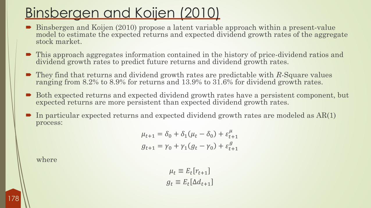
Binsbergen and Koijen (2010) Binsbergen and Koijen (2010) propose a latent variable approach within a present-value

model to estimate the expected returns and expected dividend growth rates of the aggregate stock market.

This approach aggregates information contained in the history of price-dividend ratios and dividend growth rates to predict future returns and dividend growth rates.

They find that returns and dividend growth rates are predictable with R-Square values ranging from 8.2% to 8.9% for returns and 13.9% to 31.6% for dividend growth rates.

Both expected returns and expected dividend growth rates have a persistent component, but expected returns are more persistent than expected dividend growth rates.

In particular expected returns and expected dividend growth rates are modeled as AR(1) process:

𝜇𝑡+1 = 𝛿0 + 𝛿1 𝜇𝑡 − 𝛿0 + 휀𝑡+1𝜇

𝑔𝑡+1 = 𝛾0 + 𝛾1 𝑔𝑡 − 𝛾0 + 휀𝑡+1𝑔

where

𝜇𝑡 ≡ 𝐸𝑡 𝑟𝑡+1

𝑔𝑡 ≡ 𝐸𝑡 ∆𝑑𝑡+1

178

Then

∆𝑑𝑡+1= 𝑔𝑡 + 휀𝑡+1𝑑

Plugging these equations into

𝑑𝑝𝑡 = 𝑑𝑡 − 𝑝𝑡 =𝑘

1 − 𝜌+ 𝐸𝑡

𝑗=0

∞

∆𝑑𝑡+1+𝑗 − 𝑟𝑡+1+𝑗

They get the following expression for 𝑝𝑑𝑡

𝑝𝑑𝑡 =𝑘

1 − 𝜌+𝛾0 − 𝛿01 − 𝜌

−𝜇𝑡 − 𝛿01 − 𝜌𝛿1

+𝑔𝑡 − 𝛾01 − 𝜌𝛾1

So altogether we can write the implied dynamics of the dividend-to-price ratio as:

𝑝𝑑𝑡 = 𝐴 − 𝐵1 𝜇𝑡 − 𝛿0 + 𝐵2 𝑔𝑡 − 𝛾0

where

𝐴 =𝑘

1 − 𝜌+𝛾0 − 𝛿01 − 𝜌

𝐵1 =1

1 − 𝜌𝛿1

𝐵2 =1

1 − 𝜌𝛾1179

Binsbergen and Koijen (2010)

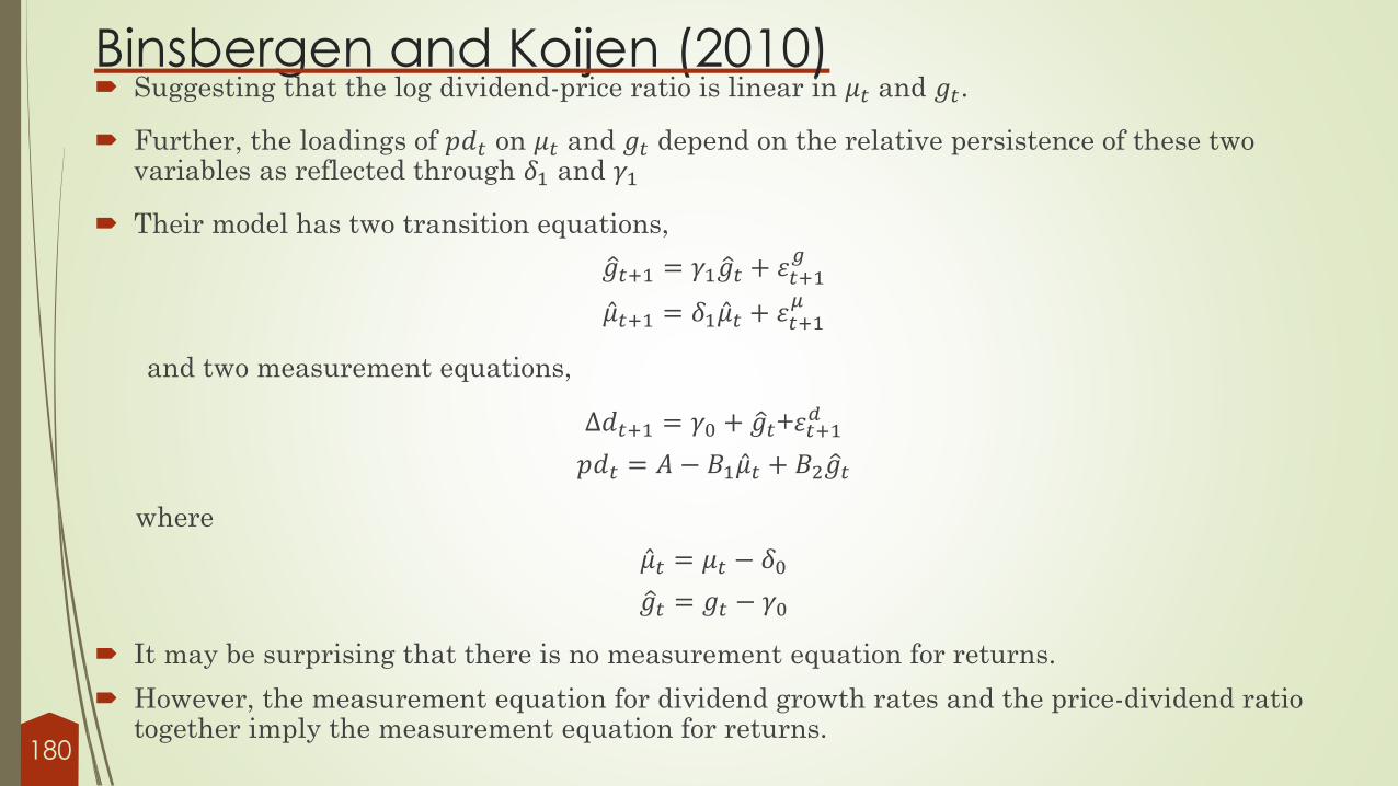
Suggesting that the log dividend-price ratio is linear in 𝜇𝑡 and 𝑔𝑡.

Further, the loadings of 𝑝𝑑𝑡 on 𝜇𝑡 and 𝑔𝑡 depend on the relative persistence of these two variables as reflected through 𝛿1 and 𝛾1

Their model has two transition equations,

ො𝑔𝑡+1 = 𝛾1 ො𝑔𝑡 + 휀𝑡+1𝑔

Ƹ𝜇𝑡+1 = 𝛿1 Ƹ𝜇𝑡 + 휀𝑡+1𝜇

and two measurement equations,

Δ𝑑𝑡+1 = 𝛾0 + ො𝑔𝑡+휀𝑡+1𝑑

𝑝𝑑𝑡 = 𝐴 − 𝐵1 Ƹ𝜇𝑡 + 𝐵2 ො𝑔𝑡

where

Ƹ𝜇𝑡 = 𝜇𝑡 − 𝛿0

ො𝑔𝑡 = 𝑔𝑡 − 𝛾0

It may be surprising that there is no measurement equation for returns.

However, the measurement equation for dividend growth rates and the price-dividend ratio together imply the measurement equation for returns.

180

Binsbergen and Koijen (2010)

Avramov, Cederburg, and Lucivjanska (2017)

They study the present value relation from a long horizon perspective.

They show that cumulative log return can be approximated as

𝑟𝑇,𝑇+𝑘 = 𝑝𝑇+𝑘 − 𝑑𝑇+𝑘 − 𝑝𝑇 − 𝑑𝑇 + σ𝑖=1𝑘 1 − 𝜌 𝑑𝑇+𝑖 − 𝑝𝑇+𝑖 + Δ𝑑𝑇,𝑇+𝑘 + 𝑘𝑞

Returns have three components that constitute the uncertainty

The difference between beginning and terminal price-to-dividend ratio 𝑝𝑇+𝑘 − 𝑑𝑇+𝑘− 𝑝𝑇 − 𝑑𝑇

The σ𝑖=1𝑘 1 − 𝜌 𝑑𝑇+𝑖 − 𝑝𝑇+𝑖 term captures the cumulative effect of dividend income

during the holding period

The Δ𝑑𝑇,𝑇+𝑘 term is the cumulative dividend growth that is realized over the horizon.

Notice that the present value relation implies restriction on the predictive framework𝑟𝑡+1Δ𝑑𝑡+1

𝑝𝑡+1 − 𝑑𝑡+1𝑧𝑡+1

= 𝑎 + 𝐵𝑝𝑡 − 𝑑𝑡𝑧𝑡

+

휀𝑟,𝑡+1휀𝑑,𝑡+1휀𝑝𝑑,𝑡+1휀𝑧,𝑡+1

181

In particular

휀𝑟,𝑡+1 = 𝜌휀𝑝𝑑,𝑡+1 + 휀𝑑,𝑡+1

The VAR thus must be estimated with observation equations for only two of the 𝑟𝑡+1, Δ𝑑𝑡+1,

and 𝑝𝑡+1 − 𝑑𝑡+1 variables to ensure that the covariance matrix is nonsingular.

Pastor, Sinha, and Swaminathan (2008) The Implied Cost of Capital (ICC) is the discount rate that equates the present value of

expected future dividends to the current stock price

One common approach is to define the ICC as the value of 𝑟𝑒 that solves

𝑃𝑡 =

𝑘=1

∞𝐸𝑡 𝐷𝑡+𝑘1 + 𝑟𝑒 𝑘

Recall that CS develop a useful approximation for the stock price which expresses the log

price 𝑝𝑡 = 𝑙𝑜𝑔 𝑃𝑡 as

𝑝𝑡 =𝑘

1 − 𝜌+ 1 − 𝜌

𝑗=0

∞

𝜌𝑗𝐸𝑡 𝑑𝑡+1+𝑗 −

𝑗=0

∞

𝜌𝑗𝐸𝑡 𝑟𝑡+1+𝑗

182

In this framework, it is natural to define the ICC as the value of 𝑟𝑒,𝑡 that solves

𝑝𝑡 =𝑘

1 − 𝜌+ 1 − 𝜌

𝑗=0

∞

𝜌𝑗𝐸𝑡 𝑑𝑡+1+𝑗 − 𝑟𝑒,𝑡

𝑗=0

∞

𝜌𝑗

To provide some insight into the ICC, it is convenient to assume that log dividend growth

𝑔𝑡+1 ≡ 𝑑𝑡+1 − 𝑑𝑡 follows a stationary AR(1) process

𝑔𝑡+1 = 𝛾 + 𝛿𝑔𝑡 + 𝜈𝑡+1, 0 < 𝛿 < 1 , 𝜈𝑡+1~𝑁 0, 𝜎𝜈2

Given these dynamics of 𝑔𝑡

𝑗=0

∞

𝜌𝑗𝐸𝑡 𝑑𝑡+1+𝑗 =

𝑑𝑡1 − 𝜌

+𝛾

1 − 𝛿 1 − 𝜌 2−

𝛾𝛿

1 − 𝛿 1 − 𝜌 1 − 𝜌𝛿+

𝛿𝑔𝑡1 − 𝜌 1 − 𝜌𝛿

Substituting this equation into 𝑝𝑡 we obtain

𝑝𝑡 =𝑘

1−𝜌+ 𝑑𝑡 +

𝛾

1−𝛿 1−𝜌−

𝛾𝛿

1−𝛿 1−𝜌𝛿+𝑔𝑡

𝛿

1−𝜌𝛿−

𝑟𝑒,𝑡

1−𝜌

183

Pastor, Sinha, and Swaminathan (2008)

which can be rearranged into

𝑟𝑒,𝑡 = 𝑘 +𝛾

1−𝛿+ 𝑑𝑡 − 𝑝𝑡 1 − 𝜌 + 𝑔𝑡 −

𝛾

1−𝛿

𝛿 1−𝜌

1−𝜌𝛿

The ICC, 𝑟𝑒,𝑡 , is a simple linear function of the log dividend-price ratio, 𝑑𝑡 − 𝑝𝑡, and log

dividend growth, 𝑔𝑡.

Further insight into the ICC can be obtained by assuming that the conditional expected

return, 𝜇𝑡 ≡ 𝐸𝑡 𝑟𝑡+1 also follows a stationary AR(1) process

𝜇𝑡+1 = 𝛼 + 𝛽𝜇𝑡 + 𝑢𝑡+1, 0 < 𝛽 < 1 , 𝑢𝑡+1~𝑁 0, 𝜎𝑢2

𝑗=0

∞

𝜌𝑗 𝐸𝑡 𝑟𝑡+1+𝑗 =𝛼

1 − 𝛽 1 − 𝜌+ 𝜇𝑡 −

𝛼

1 − 𝛽

1

1 − 𝜌𝛽

Plugging σ𝑗=0∞ 𝜌𝑗𝐸𝑡 𝑑𝑡+1+𝑗 and σ𝑗=0

∞ 𝜌𝑗 𝐸𝑡 𝑟𝑡+1+𝑗 into 𝑝𝑡, we obtain

𝑝𝑡 =𝑘

1 − 𝜌+

𝛾

1 − 𝛿 1 − 𝜌−

𝛼

1 − 𝛽 1 − 𝜌

+𝑑𝑡 + 𝑔𝑡 −𝛾

1 − 𝛿

𝛿

1 − 𝜌𝛿− 𝜇𝑡 −

𝛼

1 − 𝛽

1

1 − 𝜌𝛽184

Pastor, Sinha and, Swaminathan (2008)

The log stock price 𝑝𝑡 is a simple function of 𝑑𝑡, 𝑔𝑡 and 𝜇𝑡.

The stock price increases with dividends 𝑑𝑡 and dividend growth 𝑔𝑡, and it decreases with expected return 𝜇𝑡.

Note that 𝑝𝑡 depends on the deviations of 𝜇𝑡 and 𝑔𝑡 from their unconditional means of 𝛼

1−𝛽and

𝛾

1−𝛿respectively

Comparing the equations of 𝑝𝑡 and 𝑟𝑒,𝑡 we have

𝑟𝑒,𝑡 =𝛼

1−𝛽+ 𝜇𝑡 −

𝛼

1−𝛽

1−𝜌

1−𝜌𝛽

which implies that 𝑟𝑒,𝑡 and 𝜇𝑡 are perfectly correlated.

Thus, the ICC is a perfect proxy for the conditional expected return in the time series in an AR(1) framework

They also consider a modified version of the ICC,

𝑟𝑒2,𝑡 = 𝑘 +𝛾

1 − 𝛿+ 𝑑𝑡 − 𝑝𝑡 1 − 𝜌

185

Pastor, Sinha and, Swaminathan (2008)

This expression is obtained from the equation of 𝑟𝑒,𝑡 by setting 𝑔𝑡 equal to its

unconditional mean 𝛾

1−𝛿.

This definition of 𝑟𝑒2,𝑡 captures the idea that our information about dividend growth is

often limited in practice.

Note that 𝑟𝑒2,𝑡 is perfectly correlated with the dividend-to-price ratio, which is commonly

used to proxy for expected return.

Since dividends tend to vary less than prices, the time variation in 𝑟𝑒2,𝑡 is driven mostly

by the time variation in 𝑝𝑡.

186

Pastor, Sinha and, Swaminathan (2008)

Consumption Based Asset Pricing

Models

187

Most prominent in the class of inter-temporal models is the consumption CAPM (CCAPM).

The CCAPM is a single state variable model; real consumption growth is the single factor.

Consumption-based asset pricing models have been among the leading multi-period general

equilibrium models in financial economics for the past four decades.

The Consumption Capital Asset Pricing Model (CCAPM) was first derived in the late 1970s in

successively more general models by Rubinstein (1976), Breeden and Litzenberger (1978), and

Breeden (1979).

Lucas (1978) did not derive the CCAPM formula, yet his work on Euler equations was also

helpful to many empiricists in subsequent consumption-based asset pricing tests.

The CCAPM states that the expected excess return on any risky asset should be proportional

to its “consumption beta”, or covariation with consumption growth.

Financial assets with higher sensitivities of returns to movements in real consumption

spending have more systematic risk and should have proportionately higher excess returns

Perhaps the consumption CAPM does a better job?

188

Such assets pay off more when consumption is high and marginal utility is low, and pay

less when consumption is low and marginal utility is high, so they are worth less in price

and have higher equilibrium returns.

This CCAPM differs from the CAPM as real consumption growth is not perfectly

correlated with market returns.

In a multi-period model, market wealth can be high and still have high marginal utility if

the investment opportunity set is good, as shown by Merton (1973) and Breeden (1984).

The first two decades of CCAPM tests produced mixed results tilting towards the model

rejection

Tests of the special case of the CCAPM under constant relative risk aversion by Hansen

and Singleton (1983), Mehra and Prescott (1985), and others rejected the model.

Chen, Roll, and Ross (1986) found no significant consumption factor priced in the presence

of other factors, including industrial production, junk bond returns, and inflation hedges

Grossman, Melino, and Shiller (1987), Breeden, Gibbons, and Litzenberger (BGL, 1989)

and Wheatley (1988) examined measurement issues in consumption (such as time

aggregation) and their biases on measures of volatility and consumption betas.

The consumption CAPM

189

BGL found a significant positive coefficient on consumption betas; and separately a significant

positive coefficient on market betas; however, both the CCAPM and the CAPM were rejected.

BGL derived a useful result: estimation of consumption betas relative to returns on a

consumption mimicking portfolio, which allows greater number and frequency of observations

and more precise estimates of consumption betas.

The very strong theory in support of the CCAPM, contrasted with weak early empirical

support, motivated researchers to improve both their theoretical and empirical modeling.

On the theoretical side, Pye (1972, 1973) and Greenig (1986) developed time-multiplicative

utility functions.

Then Sundaresan (1989), Constantinides (1990), and Abel (1990) modeled habit formation.

Epstein-Zin (1989) and Weil (1989) (often jointly referred to as EZ-W) developed preference

structures that displayed time-complementarity in utility for consumption streams, allowing

researchers to separate effects of different levels of intra-temporal relative risk aversion (RRA)

from levels of the elasticity of intertemporal substitution (EIS).

The consumption CAPM

190

Campbell and Cochrane (1999) later produced a model with the habit formation approach.

With a subsistence level of consumption for a “representative individual,” their model allows

for dramatic rises in relative risk aversion as surplus consumption (above habit) goes towards

zero in severe recessions.

With the flexibility afforded by this model, they were able to fit many aspects of empirical data

on stock and bond returns as related to real consumption growth, especially the risk premium

on the stock market.

Mehra and Prescott (1985) find that the equity premium is too high (the “equity premium

puzzle”), given the low volatility of real consumption growth.

Mankiw and Zeldes (1991) considered that many households did not own stock at all or in

significant amounts, a situation called “limited participation.”

They pointed out that there is no reason that the Euler equation should hold for households

who are not investing.

They found that for households who actually owned stocks, the implied estimates of relative

risk aversion were much more reasonable than for households who did not own stocks.

Heaton and Lucas (1992, 1996) examined “incomplete markets” that did not permit full

hedging of labor income, thus causing consumers to have more volatile consumption streams.

The consumption CAPM

191

Vissing-Jorgensen (2002) focused on estimating the “elasticity of intertemporal

substitution,” which determines how much consumers change their expected consumption

growth rate when interest rates or expected returns on assets change.

She finds the EIS to be quite different for stockholders than for non-stockholders, generally

getting plausible estimates for those who chose to invest in stocks and bonds and based on

trading off current consumption versus future consumption.

Also on the empirical side, advances were made in examining changes in conditional

means, variances, and covariances and testing conditional versions of the CAPM and

CCAPM, as in Harvey (1991) and Ferson and Harvey (1991, 1999).

Lettau and Ludvigson (2001a,b) use deviations of consumption from total wealth (which

includes a human capital estimate in addition to stock market wealth) as a conditioning or

“scaling” variable for changing mean returns.

They find results quite compatible with Merton’s (1973) and Breeden’s (1984) intertemporal

theories, in that high consumption versus wealth is a predictor of future investment

returns, as consumers optimally smooth forward those changes in expected returns

The consumption CAPM

192

Lettau and Ludvigson also find significant differences in the movements of consumption betas

of value vs. growth stocks during recessions

They find that value stocks tend to have much larger increase in consumption betas during

recessions, when risks and risk premiums are high, which helps to explain the findings of

higher returns on value stocks than predicted by the unconditional CCAPM betas.

More recently, Bansal and Yaron (2004) consider the “long run risk” caused by small,

persistent shocks in the drift and volatility of real consumption growth.

They show that variance of real consumption growth grows more than proportionally with

time, which is consistent with the persistence of growth shocks.

They also provide evidence that the conditional volatility of consumption is time-varying,

which leads naturally to time-varying risk premia.

Much subsequent research has been done on this long run risk model, most notably in the

paper by Bansal, Dittmar, and Kiku (2009).

They show that aggregate consumption and aggregate dividends have a co-integrating relation

The consumption CAPM

193

They observe that “the deviation of the level of dividends from consumption (the so-called error

correction variable) is important for predicting dividend growth rates and returns at all

horizons” (1, 5 and 10 years).

Imposing co-integration allows them to predict 11.5% of the variation in 1-year returns,

whereas only 7.5% of the variation is predicted without co-integration

Their conditional consumption betas account for about 75% of the cross-sectional variation in

risk premia for the one-year horizon, and 85% for long horizons

After Grossman, Melino, and Shiller (1987) and Breeden, Gibbons, and Litzenberger (1989)

raised concerns about measuring consumption, Parker and Julliard (2005) showed that it is

important to measure “ultimate consumption betas,” since consumption changes are slow-

moving, and could take 2-3 years for the full effects to be observed.

Using measures of these ultimate consumption betas, they were able to explain much of the

Fama-French (1992) effects for size and book-to-market portfolios

Let us derive a simple discrete time version of the CCAPM

The derivation is based on the textbook treatment of Cochrane (2007).

The consumption CAPM

194

We use the power utility to describe investor preferences:

𝑢 𝑐𝑡 =1

1−𝛾𝑐𝑡1−𝛾

for 𝛾 ≠ 1,

𝑢(𝑐𝑡) = log ( 𝑐𝑡) for 𝛾 = 1.

Notation:

𝑐𝑡 denotes consumption at time 𝑡

𝛾 is the relative risk aversion parameter.

The investor must decide how to allocate her wealth between consumption and saving.

The investor can freely buy or sell any amount of a security whose current price is 𝑝𝑡 and next-

period payoff is 𝑥𝑡+1 (𝑥𝑡+1 = 𝑝𝑡+1 + 𝑑𝑡+1).

How much will she buy or sell?

To find the answer, consider (w.l.o.g.) a two-period investor whose income at time 𝑠 is 𝑒𝑠 and let 𝑦be the amount of security she chooses to buy.

A simple derivation of the consumption CAPM

195

The investor’s problem is

max𝑦

𝑢 (𝑐𝑡) + 𝔼𝑡 𝜌𝑢(𝑐𝑡+1) 𝑠. 𝑡.

𝑐𝑡 = 𝑒𝑡 − 𝑝𝑡𝑦,

𝑐𝑡+1 = 𝑒𝑡+1 + 𝑥𝑡+1𝑦,

where 𝜌 denotes the impatience parameter, also called the subjective discount factor.

Substituting the constraints into the objective, and setting the derivative with respect to y equal to zero, we obtain the first order condition for an optimal consumption and portfolio choice,

𝑝𝑡𝑢′(𝑐𝑡) = 𝔼𝑡 𝜌𝑢

′(𝑐𝑡+1)𝑥𝑡+1 .

The left hand side reflects the loss in utility from consuming less as the investor buys an additional unit of the asset.

The right hand side describes the expected increase in utility obtained from the extra payoff at 𝑡 + 1 attributed to this additional unit of the asset.

196

A simple derivation of the consumption CAPM

A well-known representation for the first order condition is obtained by dividing both sides of the

equation by 𝑝𝑡𝑢′(𝑐𝑡),

1 = 𝔼𝑡 𝜉𝑡+1𝑅𝑡+1 ,

where 𝜉𝑡+1 =𝜌𝑢′(𝑐𝑡+1)

𝑢′(𝑐𝑡)stands for the pricing kernel, also known as the marginal rate of substitution or

the stochastic discount factor, and 𝑅𝑡+1 =𝑥𝑡+1

𝑝𝑡denotes the gross return on the security.

The relation is the fundamental discount factor view of asset pricing theories.

Observe from the representation that the gross risk-free rate, the rate known at time t and

uncorrelated with the discount factor, is given by 𝑅𝑡,𝑡+1𝑓

= 1/𝔼𝑡(𝜉𝑡+1).

When investor preferences are described by the power utility function, as in equation (𝑢 𝑐𝑡=

1

1−𝛾𝑐𝑡1−𝛾

for 𝛾 ≠ 1,), the pricing kernel takes the form 𝜉𝑡+1 = 𝜌 𝑐𝑡+1/𝑐𝑡−𝛾.

Assuming lognormal consumption growth one can show that the continuously compounded risk-free rate is

𝑟𝑡,𝑡+1𝑓

= − ln( 𝜌) − ln𝔼𝑡 exp( − 𝛾Δ ln 𝑐𝑡+1) ,

= − ln ( 𝜌) + 𝛾𝔼𝑡(Δ ln 𝑐𝑡+1) −𝛾2

2𝜎𝑡2(Δ ln 𝑐𝑡+1).

197

A simple derivation of the consumption CAPM

To derive an explicit form for the risk-free rate we have used the useful relation that if 𝑥 is

normally distributed then

𝔼(𝑒𝑎𝑥) = 𝑒𝔼(𝑎𝑥)𝑒𝑎2

2𝜎2(𝑥).

We can see from the risk-free rate equation that the EIS (elasticity of inter-temporal

substitution) is 1/𝛾 which creates some problems, as discussed below.

From the fundamental representation, we also obtain a beta pricing model of the form

𝔼𝑡(𝑟𝑖,𝑡+1) = 𝑟𝑡,𝑡+1𝑓

+ −𝑐𝑜𝑣𝑡(𝑟𝑖,𝑡+1,𝜉𝑡+1)

𝑣𝑎𝑟𝑡(𝜉𝑡+1)

𝑣𝑎𝑟𝑡(𝜉𝑡+1)

𝔼𝑡(𝜉𝑡+1)

𝑟𝑖𝑠𝑘 𝑎𝑑𝑗𝑢𝑠𝑡𝑚𝑒𝑛𝑡

In words, expected excess return on each security, stock, bond, or option, should be proportional

to the coefficient in the regression of that return on the discount factor.

The constant of proportionality, common to all assets, is the risk premium

198

A simple derivation of the consumption CAPM

Focusing on the power utility function and using a first order Taylor series expansion, we obtain

𝔼(𝑟𝑖,𝑡+1) ≈ 𝑟𝑓 + 𝛽𝑖,Δ𝑐𝜆Δ𝑐,

where

𝛽𝑖,Δ𝑐 =𝑐𝑜𝑣(𝑟𝑖,𝑡+1,𝛥𝑐)

𝑣𝑎𝑟(𝛥𝑐),

𝜆Δ𝑐 = 𝛾var(Δ𝑐).

This is the discrete time version of the consumption CAPM.

The relation is exact in continuous time.

The asset’s risk is defined as the covariance between the asset return and consumption growth.

The risk premium is the product of the risk aversion and the volatility of consumption growth

Notice from the asset pricing equation that the asset expected return is larger as the covariance

between the asset return and consumption growth gets larger.

Intuition: an asset doing badly in recessions (positive covariance) when the investor consumes little,

is less desirable than an asset doing badly in expansions (negative covariance) when the investor

feels wealthy and is consuming a great deal.

The former asset will be sold for a lower price, thereby commanding higher expected return.

199

A simple derivation of the consumption CAPM

Theoretically, CCAPM Appears Preferable to the Traditional CAPM

It takes into account the dynamic nature of portfolio decisions

It integrates the many forms of wealth beyond financial asset wealth

Consumption should deliver the purest measure of good and bad times as investors consume less

when their income prospects are low or if they think future returns will be bad.

Empirically, however, the CCAPM has been unsuccessful

The Equity Premium Puzzle

From a cross section perspective, the CCAPM fails if consumption beta is unable to explain why

average returns differ across stocks, which is indeed the case.

At the aggregate level (time-series perspective) the CCAPM leads to the so-called equity premium

puzzle documented by Mehra and Prescott (1985), the risk-free rate puzzle, and the excess

volatility puzzle.

200

To illustrate, let us manipulate the first order condition: 1 = 𝔼𝑡 𝜉𝑡+1𝑅𝑡+1 (for notational clarity

I will suppress the time dependence)

1 = 𝐸(𝜉𝑅),

= 𝐸(𝜉)𝐸(𝑅) + 𝑐𝑜𝑣(𝜉, 𝑅),

= 𝐸(𝜉)𝐸(𝑅) + 𝜌𝜉,𝑅𝜎(𝜉)𝜎(𝑅).

Dividing both sides of (𝐸(𝜉)𝐸(𝑅) + 𝜌𝜉,𝑅𝜎(𝜉)𝜎(𝑅)) by 𝐸(𝜉)𝜎(𝑅) leads to

𝐸(𝑅)−𝑅𝑓

𝜎(𝑅)= −𝜌𝜉,𝑅

𝜎(𝜉)

𝐸(𝜉),

which implies that

𝐸(𝑅)−𝑅𝑓

𝜎(𝑅)≤

𝜎(𝜉)

𝐸(𝜉)= 𝜎(𝜉)𝑅𝑓 .

The left hand side is known as the Sharpe ratio.

201

The Equity Premium Puzzle

The highest Sharpe ratio is associated with portfolios lying on the efficient frontier.

Notice that the slope of the frontier is governed by the volatility of the discount factor.

Under the CCAPM it follows that

𝐸(𝑅𝑚𝑣)−𝑅𝑓

𝜎(𝑅𝑚𝑣)=

𝜎 (𝑐𝑡+1/𝑐𝑡)−𝛾

𝐸 (𝑐𝑡+1/𝑐𝑡)−𝛾 .

When log pricing kernel is normally distributed, the right hand side can be shown to be equal to

(proof in the appendix)

𝑒𝛾2𝜎2(Δ ln 𝑐𝑡+1),

which can be approximated by

𝛾𝜎(Δ ln 𝑐).

In words, the slope of the mean-variance efficient frontier is higher if the economy is riskier,

i.e., if consumption growth is more volatile or if investors are more risk averse.

Over the past several decades in the US, real stock returns have averaged 9% with a std. of

about 20%, while the real return on T-Bills has been about 1%.

202

The Equity Premium Puzzle

Thus, the historical annual market Sharpe ratio has been about 0.4.

Moreover, aggregate nondurable and services consumption growth had a std. of 1%.

This fact can only be reconciled with 𝛾=50.

But the empirical estimates are between 2 and 10.

This is the “equity premium puzzle.” The historical Sharpe ratio is simply too large than the one

obtained with reasonable risk aversion and consumption volatility estimates.

The Risk-Free Rate Puzzle

Using the standard CCAPM framework also gives rise to the risk-free rate puzzle.

Recall, we have shown that

𝑟𝑡,𝑡+1𝑓

= − ln ( 𝜌) + 𝛾𝔼𝑡(Δ ln 𝑐𝑡+1) −𝛾2

2𝜎𝑡2(Δ ln 𝑐𝑡+1)

With 𝛾=2 the risk-free rate should be around 5% to 6% per year.

The actually observed rate is less than 1%

203

The Equity Premium Puzzle

How could the Equity Premium and Risk-Free Puzzles be resolved ?

Perhaps investors are much more risk averse than we may have thought.

This indeed resolves the equity premium puzzle.

But higher risk aversion parameter implies higher risk-free rate. So higher risk aversion

reinforces the risk-free puzzle.

Perhaps the stock returns over the last 50 years are good luck rather than an equilibrium

compensation for risk.

Perhaps something is deeply wrong with the utility function specification and/or the use of

aggregate consumption data.

Indeed, the CCAPM assumes that agents’ preferences are time additive VNM representation

(e.g., power).

Standard power utility preferences impose tight restrictions on the relation between the

equity premium and the risk free rate.

As shown earlier, EIS and the relative risk aversion parameter are reciprocals of each other.

204

Economically they should not be tightly related.

EIS is about deterministic consumption paths - it measures the willingness to exchange

consumption today with consumption tomorrow for a given risk-free rate, whereas risk aversion is

about preferences over random variables.

In Epstein and Zin (1989) and Weil (1990) recursive inter-temporal utility functions, the risk

aversion is separated from the elasticity of inter-temporal substitution, thereby separating the

equity premium from the risk-free rate

Duffie and Epstein (1992) introduces the Stochastic Differential Utility which is the continuous

time version of Epstein-Zin-Weil.

They show that under certain parameter restrictions, the risk-free rate actually diminishes with

higher risk aversion.

Empirically, recursive preferences perform better in matching the data.

Reitz (1988) comes up with an interesting idea: he brings the possibility of low probability states of

economic disaster and is able to explain the observed equity premium.

Barro (2005) supports the Reitz’s perspective. i.e., the potential for rare economic disasters explains a lot of asset-

pricing puzzles including high equity premium, low risk free rate, and excess volatility.

205

How could the Equity Premium and Risk-Free Puzzles be resolved ?

Weitzman (2007) proposes an elegant solution using a Bayesian framework to characterize the ex ante

uncertainty about consumption growth.

The asset pricing literature typically assumes that the growth rate is normally distributed

𝑔 ∼ 𝑁(𝜇𝑔, 𝜎𝑔2).

The literature also assumes that 𝜇𝑔 and 𝜎𝑔 are known to the agents in the economy.

What if you assume that 𝜇𝑔 is known and 𝜎𝑔 is unknown?

Moreover, 𝜎𝑔 is a random variable obeying the inverted gamma distribution.

Then 𝑔 has the Student-t distribution. We will show this result later upon digging into

Bayesian Econometrics.

The student t distribution captures both the high equity premium and low risk-free rate.

In what follows, I will elaborate on the three most successful consumption models: long run

risk, habit formation, and prospect theory.

Beforehand, it is useful to get familiarity with the E-Z preferences.

206

How could the Equity Premium and Risk-Free Puzzles be resolved ?

Epstein and Zin follow the work by Kreps and Porteus to introduce a class of preferences

that breaks the link between risk aversion and EIS. The basic formulation is

𝑈𝑡 = 1 − 𝛽 𝐶𝑡1−

1𝜓 + 𝛽 𝐸𝑡 𝑈𝑡+1

1−𝛾

1−1𝜓

1−𝛾

1

1−1𝜓

This utility function can also be rewritten as

𝑈𝑡 = 1 − 𝛽 𝐶𝑡1−𝛾

𝜃 + 𝛽 𝐸𝑡 𝑈𝑡+11−𝛾

1

𝜃

𝜃

1−𝛾

where 𝜃 =1−𝛾

1−1

𝜓

To give some intuition, consider the case where 𝜓 = 1:

𝑈𝑡 = 1 − 𝛽 𝑙𝑜𝑔𝐶𝑡 + 𝛽𝜃 log𝐸𝑡 𝑒𝑥𝑝𝑈𝑡+1𝜃

With normally distributed 𝑈𝑡 we get that the conditional variance of utility matters:

𝑈𝑡 = 1 − 𝛽 𝑙𝑜𝑔𝐶𝑡 + 𝛽𝐸𝑡 𝑈𝑡+1 +1

2×𝛽

𝜃𝑉𝑎𝑟𝑡 𝑈𝑡+1

The first two terms correspond to the time-additive case while the third is the E-Z addition.

The Epstein-Zin preferences

207

The Euler equation of the Epstein-Zin preferences is given by,

1 = 𝐸𝑡 𝛽𝐶𝑡+1𝐶𝑡

−1𝜓

𝜃

1

𝑅𝑚,𝑡+1

1−𝜃

𝑅𝑖,𝑡+1

For the market portfolio itself, the Euler equation takes the form:

1 = 𝐸𝑡 𝛽𝐶𝑡+1𝐶𝑡

−1𝜓

𝑅𝑚,𝑡+1

𝜃

As 𝜃 = 1 this collapses to the familiar expression for power utility

Now assume that 𝐶𝑡 , 𝑅𝑚,𝑡 are jointly homoscedastic and log-normally distributed, then:

1 = 𝐸𝑡𝑒𝑥𝑝 𝜃𝑙𝑛𝛽 −𝜃

𝜓𝑙𝑛

𝐶𝑡+1𝐶𝑡

+ 𝜃𝑙𝑛𝑅𝑚,𝑡+1

208

The pricing kernel

The Epstein-Zin preferences

Notice that the form in the exponential has a normal distribution with time-varying mean (𝐸𝑡) and constant

variance, due to the homoscedasticity assumption, 𝑉 , both are given by:

𝐸𝑡 = 𝜃𝑙𝑛𝛽 −𝜃

𝜓𝐸𝑡 𝑐𝑡+1 + 𝜃𝐸𝑡𝑟𝑚,𝑡+1

𝑉 =𝜃

𝜓

2

𝜎𝑐2 + 𝜃2𝜎𝑚

2 −2𝜃2

𝜓𝜎𝑐𝑚

where 𝑐𝑡+1= 𝑙𝑛𝐶𝑡+1

𝐶𝑡

Thus,

1=𝐸𝑡𝑒𝑥𝑝 𝜃𝑙𝑛𝛽 −𝜃

𝜓𝑙𝑛

𝐶𝑡+1

𝐶𝑡+ 𝜃𝑙𝑛𝑅𝑚,𝑡+1 = 𝑒𝑥𝑝 𝐸𝑡 +

1

2𝑉

Taking logs from both sides it follows that

0 = 𝜃𝑙𝑛𝛽 −𝜃

𝜓𝐸𝑡 𝑐𝑡+1 + 𝜃𝐸𝑡𝑟𝑚,𝑡+1 +

1

2

𝜃

𝜓

2

𝜎𝑐2 + 𝜃2𝜎𝑚

2 −2𝜃2

𝜓𝜎𝑐𝑚

209

The Epstein-Zin preferences

Then we get

𝐸𝑡 𝑐𝑡+1 = 𝜇𝑚 + 𝜓𝐸𝑡𝑟𝑚,𝑡+1

where

𝜇𝑚 = 𝜓𝑙𝑛𝛽 +1

2

𝜃

𝜓𝑉𝑎𝑟𝑡 𝑐𝑡+1 − 𝜓𝑟𝑚,𝑡+1

We can also understand the cross section of returns: the pricing kernel representation is

𝐸𝑡𝑒𝑥𝑝 𝜃𝑙𝑛𝛽 −𝜃

𝜓𝑙𝑛

𝐶𝑡+1

𝐶𝑡+ 𝜃 − 1 𝑙𝑛𝑅𝑚,𝑡+1 + 𝑙𝑛𝑅𝑖,𝑡+1 =1

Then expected return is given by

𝐸𝑡 𝑟𝑖,𝑡+1 − 𝑟𝑓,𝑡+1 = −𝜎𝑖2

2+ 𝜃

𝜎𝑖𝑐𝜓

+ 1 − 𝜃 𝜎𝑖𝑚

210

The Epstein-Zin preferences

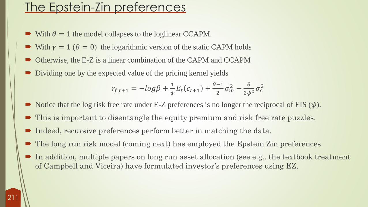
With 𝜃 = 1 the model collapses to the loglinear CCAPM.

With 𝛾 = 1 (𝜃 = 0) the logarithmic version of the static CAPM holds

Otherwise, the E-Z is a linear combination of the CAPM and CCAPM

Dividing one by the expected value of the pricing kernel yields

𝑟𝑓,𝑡+1 = −𝑙𝑜𝑔𝛽 +1

𝜓𝐸𝑡 𝑐𝑡+1 +

𝜃−1

2𝜎𝑚2 −

𝜃

2𝜓2 𝜎𝑐2

Notice that the log risk free rate under E-Z preferences is no longer the reciprocal of EIS (𝜓).

This is important to disentangle the equity premium and risk free rate puzzles.

Indeed, recursive preferences perform better in matching the data.

The long run risk model (coming next) has employed the Epstein Zin preferences.

In addition, multiple papers on long run asset allocation (see e.g., the textbook treatment

of Campbell and Viceira) have formulated investor’s preferences using EZ.

211

The Epstein-Zin preferences

The Long Run Risk model The LRR of Bansal and Yaron (2004) has been one of the most successful asset

pricing theory over the last decade.

LRR models feature a small but highly persistent component in consumption growth

that is hard to capture directly using consumption data.

Never-the-less that small component is important for asset pricing.

The persistent component is modeled either as stationary (Bansal and Yaron (2004))

or as co-integrated (Bansal, Dittmar, and Kiku (2009)) stochastic process.

The model has been found useful in explaining the equity premium puzzle, size and

book to market effects, momentum, long term reversals, risk premiums in bond

markets, real exchange rate movements, among others (see a review paper by

Bansal (2007)).

The evidence is based on calibration experiments.

212

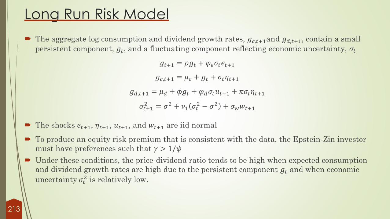
The aggregate log consumption and dividend growth rates, 𝑔𝑐,𝑡+1and 𝑔𝑑,𝑡+1, contain a small

persistent component, 𝑔𝑡, and a fluctuating component reflecting economic uncertainty, 𝜎𝑡

𝑔𝑡+1 = 𝜌𝑔𝑡 + 𝜑𝑒𝜎𝑡𝑒𝑡+1

𝑔𝑐,𝑡+1 = 𝜇𝑐 + 𝑔𝑡 + 𝜎𝑡𝜂𝑡+1

𝑔𝑑,𝑡+1 = 𝜇𝑑 + 𝜙𝑔𝑡 + 𝜑𝑑𝜎𝑡𝑢𝑡+1 + 𝜋𝜎𝑡𝜂𝑡+1

𝜎𝑡+12 = 𝜎2 + 𝜈1 𝜎𝑡

2 − 𝜎2 + 𝜎𝑤𝑤𝑡+1

The shocks 𝑒𝑡+1, 𝜂𝑡+1, 𝑢𝑡+1, and 𝑤𝑡+1 are iid normal

To produce an equity risk premium that is consistent with the data, the Epstein-Zin investor

must have preferences such that 𝛾 > 1/𝜓

Under these conditions, the price-dividend ratio tends to be high when expected consumption

and dividend growth rates are high due to the persistent component 𝑔𝑡 and when economic

uncertainty 𝜎𝑡2 is relatively low.

Long Run Risk Model

213

Bansal and Yaron consider the E-Z pricing kernel representation derived earlier

𝐸𝑡𝑒𝑥𝑝 𝜃𝑙𝑛𝛽 −𝜃

𝜓𝑙𝑛

𝐶𝑡+1

𝐶𝑡+ 𝜃 − 1 𝑙𝑛𝑅𝑚,𝑡+1 + 𝑙𝑛𝑅𝑖,𝑡+1 =1

Their notation : 𝐸𝑡𝑒𝑥𝑝 𝜃𝑙𝑛𝛿 −𝜃

𝜓𝑔𝑡+1 + 𝜃 − 1 𝑟𝑎,𝑡+1 + 𝑟𝑖,𝑡+1 =1

Notice that 𝑟𝑎,𝑡+1is the log return on as asset that delivers aggregate consumption as its

dividends each period.

Need to solve for 𝑟𝑎,𝑡+1using the Campbell-Shiller present value formula to be developed here

𝑟𝑎,𝑡+1 = 𝑘0 + 𝑘1𝑧𝑡+1 − 𝑧𝑡 + 𝑔𝑡+1

where z is the log price-to-dividend ratio.

Then they guess 𝑧𝑡 = 𝐴0 + 𝐴1𝑥𝑡 + 𝐴2𝜎𝑡2 and substitute this into the Euler equation.

Long Run Risk Model

214

Ferson, Nallareddy, and Xie (2011) examine the out of sample performance of the LRR

paradigm.

They examine both the stationary and co-integrated versions of the model.

They find that the model performs comparably overall to the simple CAPM as well as a co-

integrated version outperforms the stationary version.

Beeler and Campbell (2012) display several weaknesses of LRR models:

Too strong predictability of consumption growth by the price-dividend ratio

Too small variance risk premium

Too strong predictive power of return volatility by the price-dividend ratio

Too small discount rate risk versus cash flow risk

In response, Zhou and Zhu (2013) propose an extra volatility factor that helps resolve these

weaknesses

Long Run Risk Model

215

The habit formation model In the literature on habit formation there are two types of models that govern the

specification of the habit level.

In the internal habit models, habit is a function of previous consumption path.

In the external habit models, habit is a function of the consumption of a peer group

or the aggregate consumption

Another modelling twist is about how consumption is related to the habit level.

Abel (1990) and Chan and Kogan (2002) are examples of ratio models in which

utility is defined over the ratio of consumption to habit

Constantinides (1990) and Campbell and Cochrane (1999) are examples of

difference models wherein utility is defined over the difference between

consumption and habit.

Importantly, the relative risk aversion is constant in ratio models but time-varying

in difference models.

216

The habit formation model

Time-varying relative risk aversion implies that the price of risk is time-varying

This feature lines up with the ever growing literature on time-series predictability.

In difference habit models, expected returns are time varying due to changes in the effective

risk aversion of the agents as we show below.

Following extended periods of low consumption growth, investors require higher risk

premiums as consumption approaches the habit.

This variation in discount rates in the model produces stock market returns that are

predictable using the price-dividend ratio

In the Campbell and Cochrane (1999) model, agents in the model maximize expected utility

𝐸

𝑡+1

∞

𝛿𝑡𝐶𝑡 − 𝐻𝑡

1−𝛾

1 − 𝛾

where 𝐶𝑡 is consumption and 𝐻𝑡 is the habit level

217

Aggregate consumption growth and dividend growth follow lognormal processes,

𝑙𝑜𝑔 𝐶𝑡+1/𝐶𝑡 = 𝑔𝑐 + 𝜎𝑐𝜂𝑡+1𝑙𝑜𝑔 𝐷𝑡+1/𝐷𝑡 = 𝑔𝑑 + 𝜎𝑑𝜖𝑡+1

where 𝐷𝑡+1 is the aggregate dividend on stocks. The innovations 𝜂𝑡+1 and 𝜖𝑡+1 are iid and come

from a standard bivariate normal distribution with correlation 𝜔

The consumption of the identical agents must equal aggregate consumption in equilibrium,

𝐶𝑡 = 𝐶𝑡

The surplus ratio is the sole state variable that describes time variation in valuation levels and

expected returns in the model.

The price-dividend ratio is an increasing function of the surplus ratio

Expected returns are decreasing in the surplus of consumption over the habit level.

Expected returns are thus a decreasing function of the price-dividend ratio218

The habit formation model

The evolution of the habit can be described by the log surplus ratio

𝑠𝑡 = 𝑙𝑜𝑔𝐶𝑡 − 𝐻𝑡

𝐶𝑡

which measures the surplus of aggregate consumption over the habit level

The log surplus ratio follows the process

𝑠𝑡+1 = 1 − 𝜙 𝑠 + 𝜙𝑠𝑡 + 𝜆 𝑠𝑡 𝑐𝑡+1 − 𝑐𝑡 − 𝑔𝑐

where 𝜙 governs the persistence and 𝑠 governs the long-run mean of the log surplus ratio, 𝑔𝑐 is expected

consumption growth, and 𝜆 𝑠𝑡 is a sensitivity function that modulates the effect of unexpected consumption

growth on the habit.

219

The habit formation model

In what follows, it is useful to consult the class notes by Simone Gilchrise: ‘Asset pricing

models with Habit Formation’

Campbell and Cochrane use the following sensitivity function:

𝜆 𝑠𝑡 =1

𝑆1 − 2 𝑠𝑡 − 𝑠 − 1

where 0 ≤ 𝑆 ≤ 𝑠𝑚𝑎𝑥 and 𝑆 and smax are respectively the steady-state and upper bound of the

surplus-consumption ratio given by

𝑆 = 𝜎𝛾

1−𝜙

𝑠𝑚𝑎𝑥 = 𝑠 +1 − 𝑆

2

2

These two values for 𝑆 and smax are one possible choice that Campbell and Cochrane justify to

make the habit locally predetermined.

220

The habit formation model

This sensitivity function allows them to have a constant risk-free interest rate.

To see this, note that the risk-free rate is

𝑟𝑡+1𝑓

= −𝑙𝑜𝑔𝛽 + 𝛾𝑔 − 𝛾 1 − 𝜙 𝑠𝑡 − 𝑠 −𝛾2𝜎2

21 + 𝜆 𝑠𝑡

2

Two effects where 𝑠𝑡 appears: intertemporal substitution and precautionary savings.

When 𝑠𝑡 is low, households have a low IES which drives the risk free rate up.

High risk aversion induces more precautionary savings which drives the risk free rate down

Campbell and Cochrane offset these two effects by picking λ such that

𝛾 1 − 𝜙 𝑠𝑡 − 𝑠 +𝛾2𝜎2

21 + 𝜆 𝑠𝑡

2= 𝑐𝑜𝑛𝑠𝑡𝑎𝑛𝑡

If agent’s utility is 𝜐 𝐶, 𝐻 = 𝑢 𝐶 − 𝐻 instead of 𝑢 𝐶 and 𝐻 grows over time so that its

distance to 𝐶 is always rather small, then a given percentage change in 𝐶 generates a larger

percentage change in 𝐶 − 𝐻 :Δ 𝐶 − 𝐻

𝐶 − 𝐻=Δ𝐶

𝐶

𝐶

𝐶 − 𝐻>Δ𝐶

𝐶221

The habit formation model

This is just a “leverage” effect coming from the “subsistence level” 𝐻.

Hence for a given volatility of 𝐶, we get more volatility of marginal utility of consumption 𝒹𝑢

𝒹𝐶.

This allows to come closer to the Hansen-Jagannathan bounds: marginal utility of

consumption is volatile, which is essential to resolve the equity premium puzzle.

When agents’ consumption becomes closer to the habit level h, they fear further negative

shocks since their utility is concave

The relative risk aversion is time varying:

RRA 𝐶 =−𝐶𝜈′′ 𝐶

𝜈′ 𝐶=

−𝐶𝑢′′ 𝐶−𝐻

𝑢′ 𝐶−𝐻

With preferences given by 𝑢 𝐶 =𝐶1−𝛾

1−𝛾, direct calculation yields

RRA 𝐶 = = 𝛾𝐶

𝐶−𝐻

As C → H, RRA 𝐶 =→∞.

Hence “time-varying risk aversion”, and hence time-varying risk premia

222

The habit formation model

Key mechanism

Time-varying local risk-aversion coefficient:

𝛾𝑡 = −𝐶𝑈𝐶𝐶𝑈𝐶

=𝛾

𝑆𝑡

Counter-cyclical market price of risk.

To show it, let us start from

𝑆𝑅𝑡 =𝐸𝑡 𝑅𝑡+1

𝑒

𝜎𝑡 𝑅𝑡+1𝑒 ≤

𝜎𝑡 𝑀𝑡+1

𝐸𝑡 𝑀𝑡+1= 𝑀𝑃𝑅𝑡

𝑀𝑃𝑅𝑡 is the market price of risk.

As noted earlier, equality holds for assets that are perfectly correlated with the SDF.

In this model the market price of risk is:

𝑀𝑃𝑅𝑡 = 𝛾𝜎 1 + 𝜆 𝑠𝑡 =𝛾𝜎

𝑆1 − 2 𝑠𝑡 − 𝑠

At the steady-state, 𝑆𝑅 =𝛾𝜎

𝑆, but the market price of risk is countercyclical, and hence so is

the Sharpe ratio.223

Several more insights:

Volatility of returns is higher in bad times

The model also matches the time-series predictability evidence: dividend growth is not

predictable, but returns are predictable, and the volatility of the price-to-dividend ratio

is accounted for by this latter term (“discount rate news”).

Long-run equity premium: because of mean-reversion in stock prices, excess returns on

stocks at long horizons are even more puzzling than the standard one-period ahead

puzzle.

Campbell and Cochrane note that if the state variable is stationary, the long-run

standard deviation of the SDF will not depend on the current state. Key point: in their

model, 𝑆−𝛾 is not stationary – variance is growing with horizon!

224

Key mechanism

The prospect theory model

In the prospect theory model of Barberis et al. (2001), identical agents extract utility not only from their consumption but also from fluctuations in their financial wealth.

Prospect theory investors are loss averse, as they are more concerned about losses than gains.

Investors track their gains and losses relative to a slow-moving benchmark, and their effective risk aversion is higher (lower) when they have accumulated losses (gains).

This specification triggers intertemporal variation in risk aversion and more volatile asset prices relative to the benchmark case with symmetric preferences

Formally, prospect theory agents maximize utility of the form

𝐸

𝑡+1

∞

𝛿𝑡𝐶𝑡1−𝛾

1 − 𝛾+ 𝑏0𝐶𝑡

−𝛾𝛿𝑡+1𝜐 Χ𝑡+1, 𝑆𝑡 , 𝑠𝑡

∗

The first part of the utility function corresponds to standard power utility over the agent's consumption

The second part reflects loss aversion preferences

The 𝑏0𝐶𝑡−𝛾

term is a scaling factor

225

The function 𝜐 depends on

The value of the agent's stock holdings 𝑆𝑡

The change in financial wealth 𝑋𝑡+1 ≡ 𝑆𝑡𝑅𝑡+1 − 𝑆𝑡𝑅𝑓,𝑡 (where 𝑅𝑡+1 and 𝑅𝑓,𝑡 are the returns on stocks and the risk-free asset)

𝑠𝑡∗ which is the historical benchmark level of stocks 𝑆𝑡

∗ given as a fraction of the stock value 𝑆𝑡(i.e., 𝑠𝑡

∗ ≡ 𝑆𝑡∗/𝑆𝑡)

The state variable 𝑠𝑡∗ is assumed to sluggishly evolve and is modeled by

𝑠𝑡+1∗ = 𝜂 𝑠𝑡

∗𝑅

𝑅𝑡+1+ 1 − 𝜂

which 𝑅 is a parameter chosen such that 𝑠𝑡∗ is equal to one on average

𝜂 ∈ 0,1 corresponds to the memory of the agents

If 𝜂 = 0 the benchmark level quickly adapts and is equal to the stock price at every time t, 𝑆𝑡∗ = 𝑆𝑡

When 𝜂 is greater than zero, however, the benchmark level reflects a longer memory of the agent with respect to past gains and losses

226

The prospect theory model

Overall, the function 𝜐 captures loss aversion such that agents are more sensitive to losses below

their historical benchmark.

Aggregate consumption and dividend growth rates follow the same iid processes as in the habit

formation model

𝑙𝑜𝑔 𝐶𝑡+1/𝐶𝑡 = 𝑔𝑐 + 𝜎𝑐𝜂𝑡+1𝑙𝑜𝑔 𝐷𝑡+1/𝐷𝑡 = 𝑔𝑑 + 𝜎𝑑𝜖𝑡+1

Given that dividend growth is IID, all variation in the price-dividend ratio is driven through a

valuation channel with time-varying expected returns.

For example, the gains from an unexpected positive dividend shock reduce effective risk

aversion.

A corresponding decrease in expected returns is accompanied by an increase in the price-

dividend ratio that amplifies the effects of dividend shocks in the model.

In equilibrium, the price-dividend ratio and expected returns are functions of the sole state

variable 𝑠𝑡∗.

227

The prospect theory model

When prospect theory meets data Barberis, Mukherjee, and Wang (2015) develop testable predictions of prospect theory.

They outline the challenges in applying prospect theory outside the laboratory.

In particular, prospect theory entails two steps.

First, since a prospect theory agent is assumed to derive utility from gains and losses, the agent forms a mental representation of the gains and losses characterizing the random outcome.

In experimental settings, the answer is clear: laboratory subjects are typically given a representation for any risk they are asked to consider – a 50:50 bet to win $110 or lose $100, say.

Outside the laboratory, however, the answer is less clear: how does an investor who is thinking about a stock represent that stock in his mind?

Second, the agent evaluates this representation – this distribution of gains and losses –to see if it is appealing.

The valuation step is straightforward: Tversky and Kahneman (1992) provide detailed formulas that specify the value that a prospect theory agent would assign to any given distribution of gains and losses.

228

When prospect theory meets data

Barberis et al suggest that, for many investors, their mental representation of a

stock is given by the distribution of the stock’s past returns.

Indeed, the past return distribution is a good and easily accessible proxy for the

object agents are interested in - the distribution of the stock’s future returns.

This belief may be mistaken: a stock with a high mean return over the past few

years typically could have low subsequent return (De Bondt and Thaler, 1985);

and a stock whose past returns are highly skewed need not exhibit high

skewness in its future returns.

Nonetheless, many investors may think that a stock’s past return distribution is

a good approximation of its future return distribution, and therefore adopt the

past return distribution as their mental representation of the stock.

229