Topic19 Image Coding-II
53
ECE ECE - - G311 G311 2 2 - - D Signal and Image Processing D Signal and Image Processing Image Coding Image Coding - - II II
-
Upload
miguel-alejandro -
Category
Documents
-
view
163 -
download
2
Transcript of Topic19 Image Coding-II
ECEECE--G311G311
22--D Signal and Image ProcessingD Signal and Image Processing
Image CodingImage Coding--IIII
ECE G311 – Image Coding-II Slide 2 of 36
OutlineOutlineWaveform Coding
Pixel CodingPCM
Entropy CodingHuffmanGroup CodingLZW Coding
Predictive CodingDelta ModulationLine-by-Line DPCM2D DPCMLossless DPCM
ECE G311 – Image Coding-II Slide 3 of 36
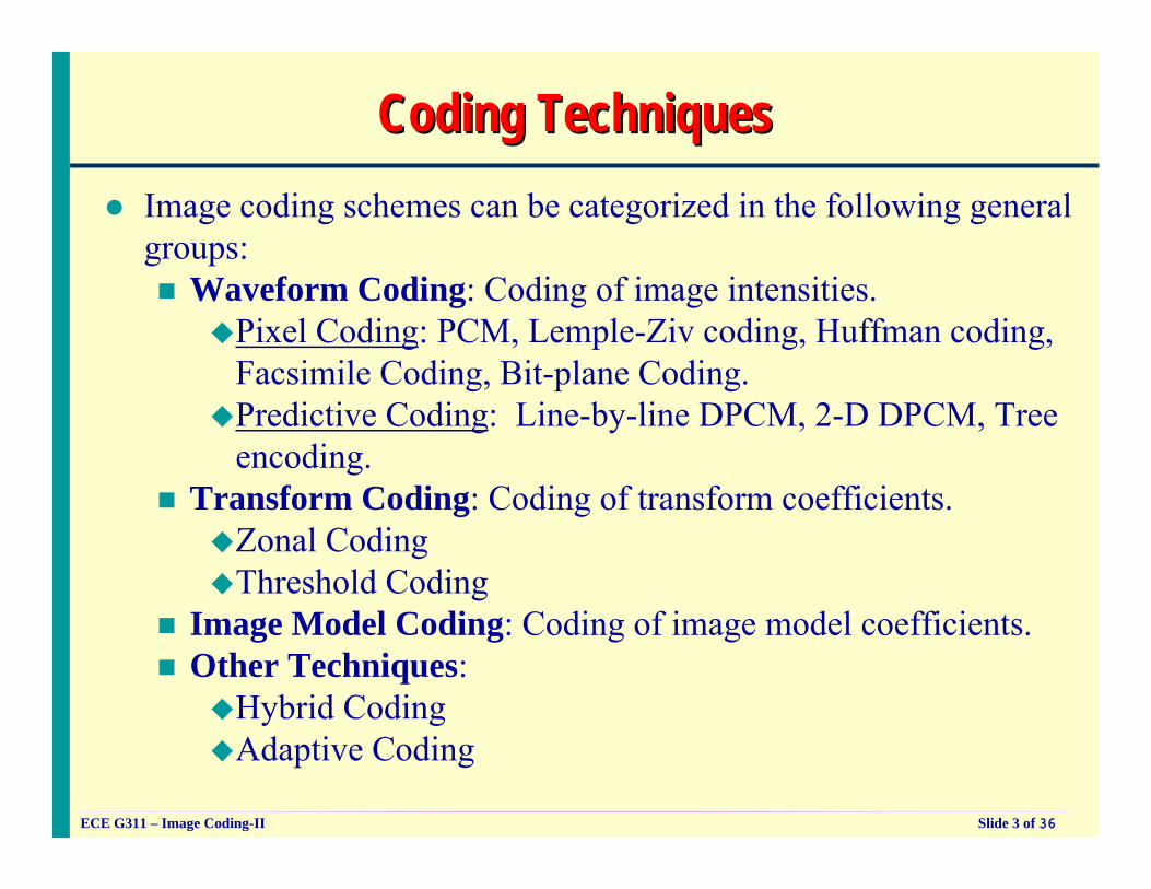
Coding TechniquesCoding TechniquesImage coding schemes can be categorized in the following generalgroups:
Waveform Coding: Coding of image intensities.Pixel Coding: PCM, Lemple-Ziv coding, Huffman coding, Facsimile Coding, Bit-plane Coding.Predictive Coding: Line-by-line DPCM, 2-D DPCM, Tree encoding.
Transform Coding: Coding of transform coefficients.Zonal CodingThreshold Coding
Image Model Coding: Coding of image model coefficients.Other Techniques:
Hybrid CodingAdaptive Coding
ECE G311 – Image Coding-II Slide 4 of 36
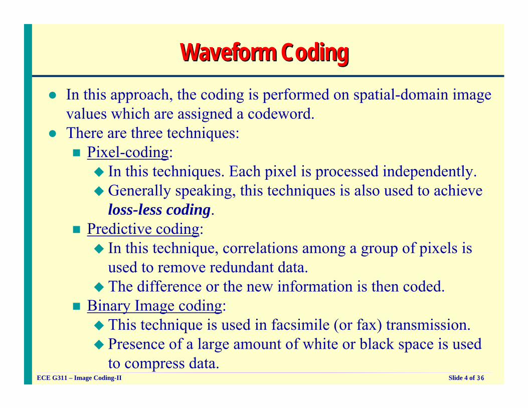
Waveform CodingWaveform CodingIn this approach, the coding is performed on spatial-domain image values which are assigned a codeword.There are three techniques:
Pixel-coding:In this techniques. Each pixel is processed independently.Generally speaking, this techniques is also used to achieve loss-less coding.
Predictive coding:In this technique, correlations among a group of pixels is used to remove redundant data.The difference or the new information is then coded.
Binary Image coding:This technique is used in facsimile (or fax) transmission.Presence of a large amount of white or black space is used to compress data.
ECE G311 – Image Coding-II Slide 5 of 36
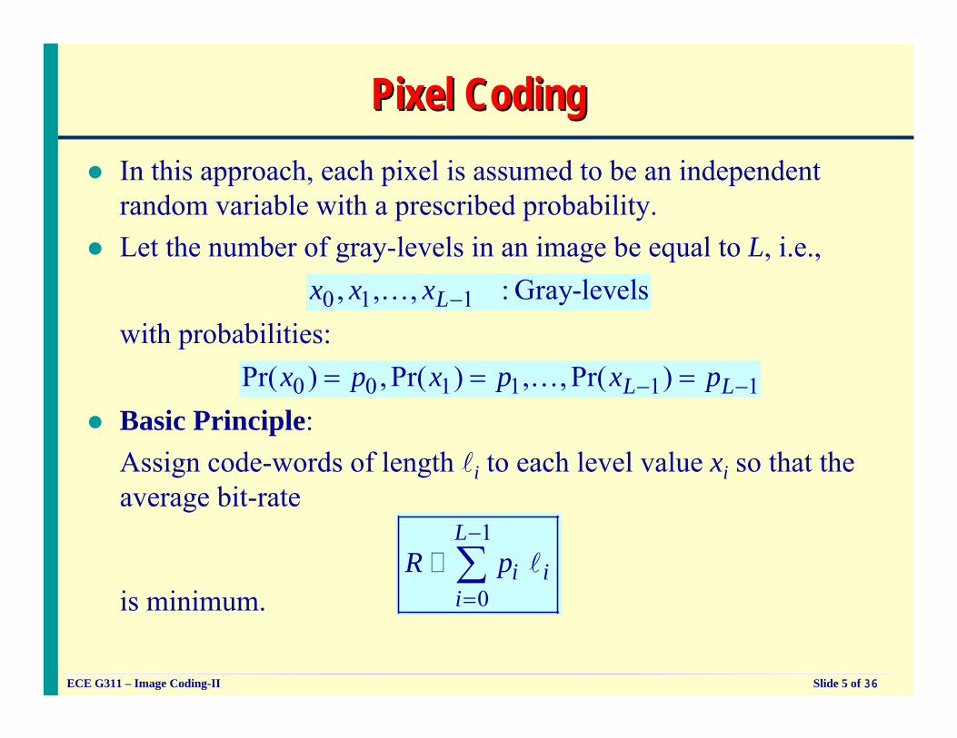
Pixel CodingPixel CodingIn this approach, each pixel is assumed to be an independent random variable with a prescribed probability.Let the number of gray-levels in an image be equal to L, i.e.,
with probabilities:
Basic Principle:Assign code-words of length li to each level value xi so that the average bit-rate
is minimum.
0 1 1, , , : Gray-levelsLx x x −K
0 0 1 1 1 1Pr( ) , Pr( ) , , Pr( )L Lx p x p x p− −= = =K
1
0
L
i ii
R p−
=∑ l
ECE G311 – Image Coding-II Slide 6 of 36
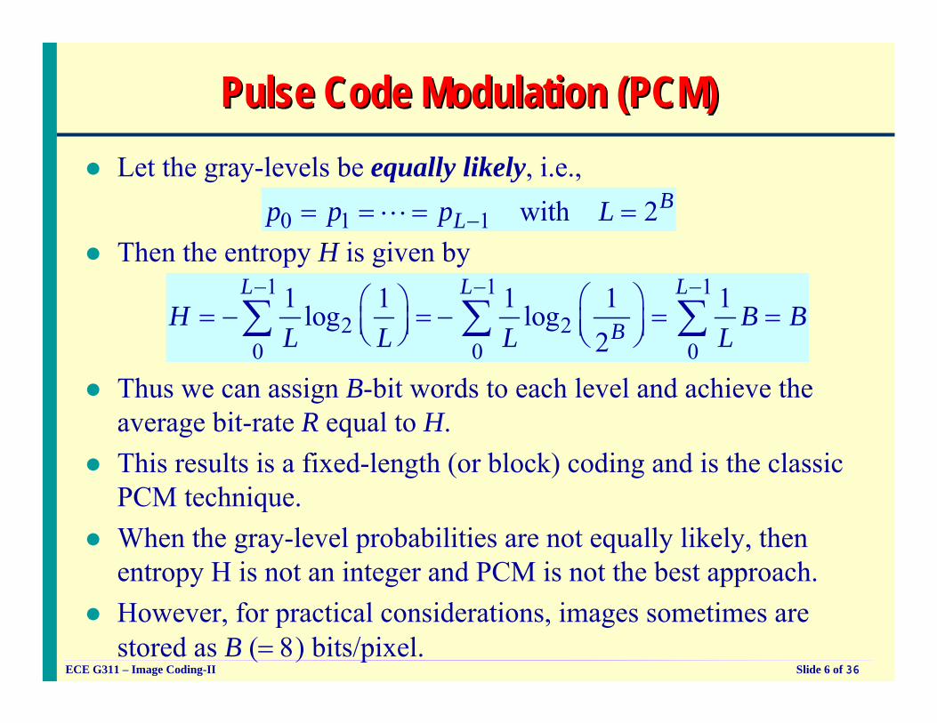
Pulse Code Modulation (PCM)Pulse Code Modulation (PCM)Let the gray-levels be equally likely, i.e.,
Then the entropy H is given by
Thus we can assign B-bit words to each level and achieve the average bit-rate R equal to H.This results is a fixed-length (or block) coding and is the classic PCM technique.When the gray-level probabilities are not equally likely, then entropy H is not an integer and PCM is not the best approach.However, for practical considerations, images sometimes are stored as B (= 8) bits/pixel.
0 1 1 with 2BLp p p L−= = = =L
1 1 1
2 20 0 0
1 1 1 1 1log log2
L L L
BH B BL L L L
− − −⎛ ⎞⎛ ⎞= − = − = =⎜ ⎟ ⎜ ⎟⎝ ⎠ ⎝ ⎠∑ ∑ ∑
ECE G311 – Image Coding-II Slide 7 of 36
Entropy CodingEntropy CodingWhat we need a variable length coding technique that can assign a uniquely decodable (prefix-free) code-words to achieve bit-rate R very close to the entropy H.Such techniques are called Entropy Coding techniques.The best optimal solution of attaining R to H was proposed by David Huffman (1950) as a part of his term project in the Information theory class at MIT. It is now known as Huffman coding technique.Huffman’s trick, in today’s jargon, was to “think outside the box.”He studied binary code tree to establish properties that an optimal prefix-free code should have.These few properties led to a simple recursive procedure for constructing an optimal code.
ECE G311 – Image Coding-II Slide 8 of 36
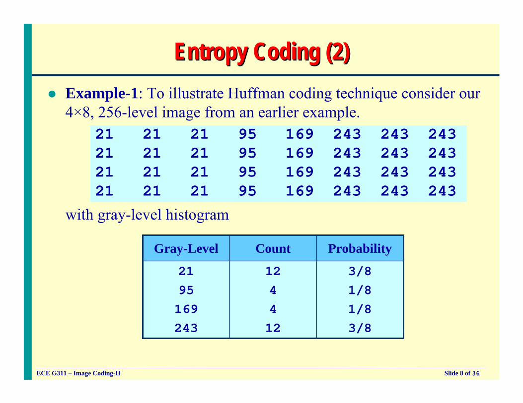
Entropy Coding (2)Entropy Coding (2)Example-1: To illustrate Huffman coding technique consider our 4×8, 256-level image from an earlier example.
21 21 21 95 169 243 243 24321 21 21 95 169 243 243 24321 21 21 95 169 243 243 24321 21 21 95 169 243 243 243
with gray-level histogram
3/81/81/83/8
1244
12
2195
169243
ProbabilityCountGray-Level
ECE G311 – Image Coding-II Slide 9 of 36
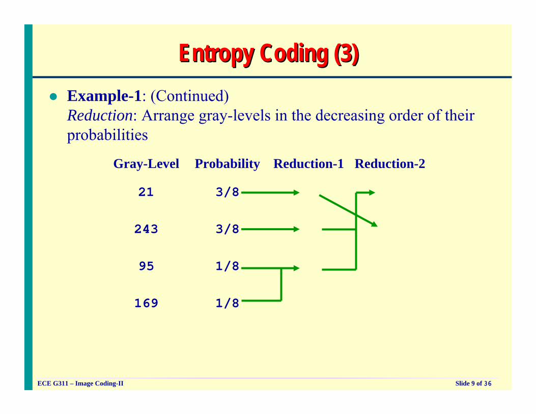
Entropy Coding (3)Entropy Coding (3)Example-1: (Continued)Reduction: Arrange gray-levels in the decreasing order of their probabilities
1/8169
1/41/895
3/83/83/8243
5/83/83/821
Reduction-2Reduction-1ProbabilityGray-Level
ECE G311 – Image Coding-II Slide 10 of 36
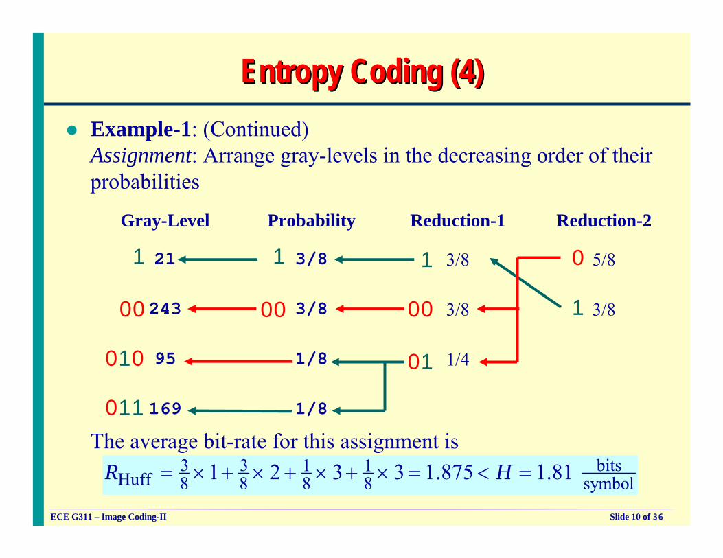
Entropy Coding (4)Entropy Coding (4)Example-1: (Continued)Assignment: Arrange gray-levels in the decreasing order of their probabilities
1/8169
1/41/895
3/83/83/8243
5/83/83/821
Reduction-2Reduction-1ProbabilityGray-Level
0
1
11 1
00
01
0000
010
011
The average bit-rate for this assignment is3 3 bits1 1
Huff 8 8 8 8 symbol1 2 3 3 1.875 1.81 R H= × + × + × + × = < =
ECE G311 – Image Coding-II Slide 11 of 36
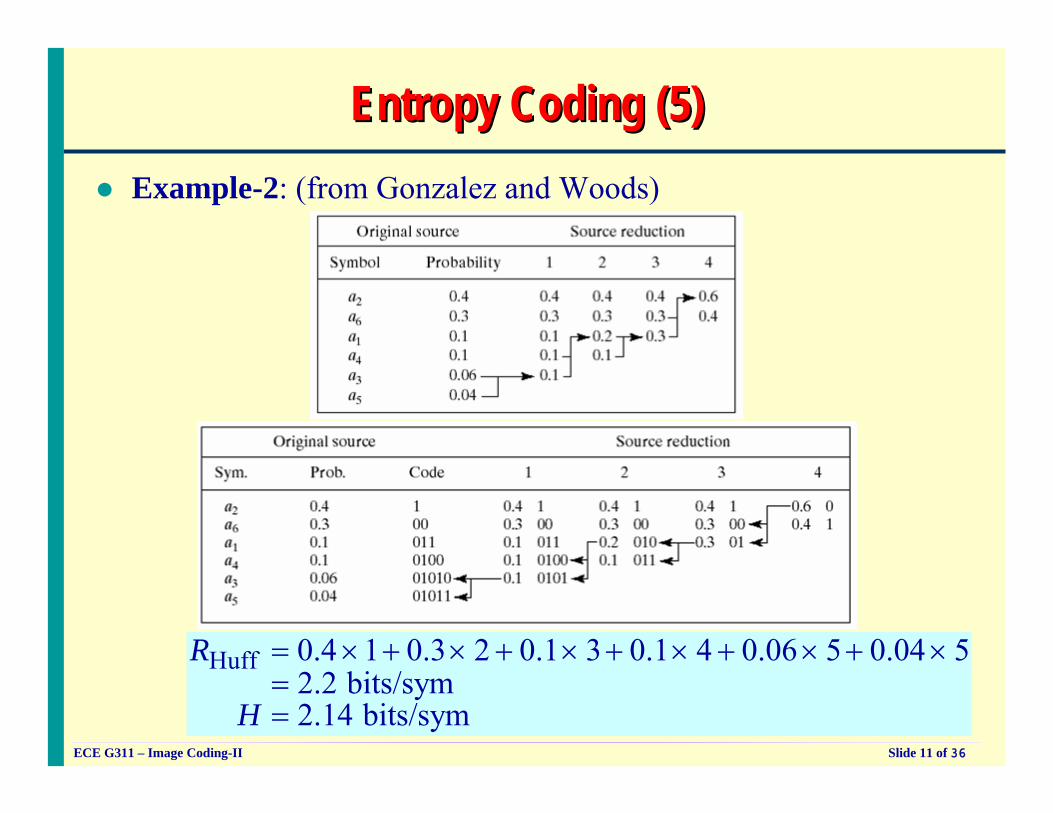
Entropy Coding (5)Entropy Coding (5)Example-2: (from Gonzalez and Woods)
Huff 0.4 1 0.3 2 0.1 3 0.1 4 0.06 5 0.04 52.2 bits/sym2.14 bits/sym
R
H
= × + × + × + × + × + ×==
ECE G311 – Image Coding-II Slide 12 of 36
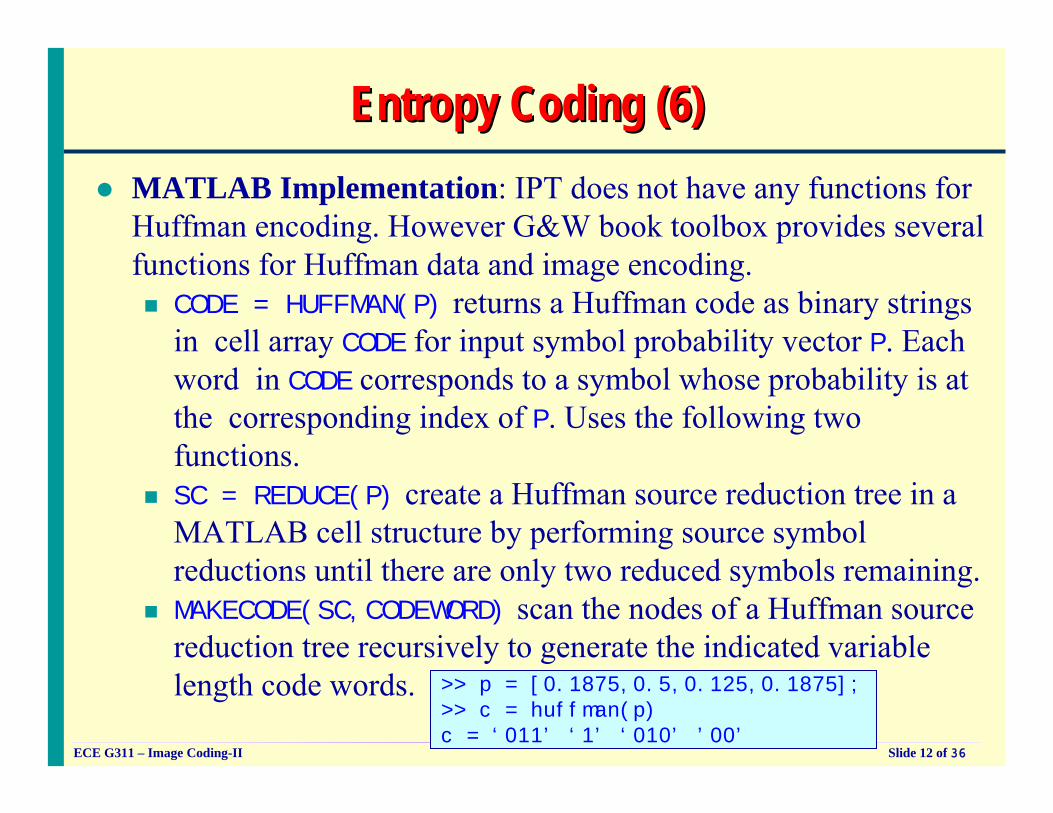
Entropy Coding (6)Entropy Coding (6)MATLAB Implementation: IPT does not have any functions for Huffman encoding. However G&W book toolbox provides several functions for Huffman data and image encoding.
CODE = HUFFMAN(P) returns a Huffman code as binary strings in cell array CODE for input symbol probability vector P. Each word in CODE corresponds to a symbol whose probability is at the corresponding index of P. Uses the following two functions.SC = REDUCE(P) create a Huffman source reduction tree in a MATLAB cell structure by performing source symbol reductions until there are only two reduced symbols remaining.MAKECODE(SC,CODEWORD) scan the nodes of a Huffman source reduction tree recursively to generate the indicated variable length code words. >> p = [0.1875,0.5,0.125,0.1875];
>> c = huffman(p)c = ‘011’ ‘1’ ‘010’ ’00’
ECE G311 – Image Coding-II Slide 13 of 36
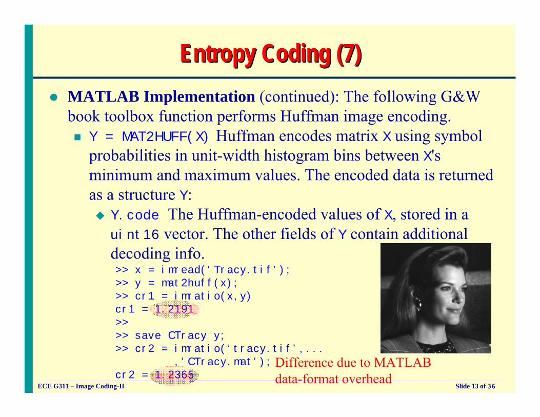
Entropy Coding (7)Entropy Coding (7)MATLAB Implementation (continued): The following G&W book toolbox function performs Huffman image encoding.
Y = MAT2HUFF(X) Huffman encodes matrix X using symbol probabilities in unit-width histogram bins between X's minimum and maximum values. The encoded data is returned as a structure Y:
Y.code The Huffman-encoded values of X, stored in a uint16 vector. The other fields of Y contain additional decoding info.>> x = imread(‘Tracy.tif’); >> y = mat2huff(x);>> cr1 = imratio(x,y)cr1 = 1.2191>>>> save CTracy y;>> cr2 = imratio(‘tracy.tif’,...
,’CTracy.mat’);cr2 = 1.2365
Difference due to MATLAB data-format overhead
ECE G311 – Image Coding-II Slide 14 of 36
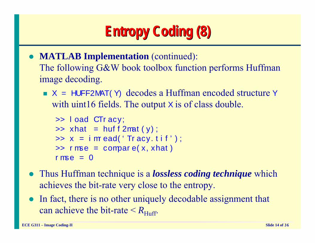
Entropy Coding (8)Entropy Coding (8)MATLAB Implementation (continued): The following G&W book toolbox function performs Huffman image decoding.
X = HUFF2MAT(Y) decodes a Huffman encoded structure Ywith uint16 fields. The output X is of class double.>> load CTracy;>> xhat = huff2mat(y);>> x = imread(‘Tracy.tif’);>> rmse = compare(x,xhat)rmse = 0
Thus Huffman technique is a lossless coding technique which achieves the bit-rate very close to the entropy.In fact, there is no other uniquely decodable assignment that can achieve the bit-rate < RHuff.
ECE G311 – Image Coding-II Slide 15 of 36
Entropy Coding (9)Entropy Coding (9)Disadvantage:
For a large number of levels, this scheme is time consuming.For example, if L = 256 (8-bit image) then we will need 254 source reductions and then 254 code-word assignments.If the probability distribution changes, then we will have to repeat this procedure.
Therefore, in practice, we consider other variable-length coding schemes that are suboptimal yet simple to implement.Truncated Huffman Coding:
In this approach, most probable L1 < L levels are Huffman coded.The remaining (L – L1) levels are coded using a prefix-code followed by a suitable fixed-length code.
ECE G311 – Image Coding-II Slide 16 of 36
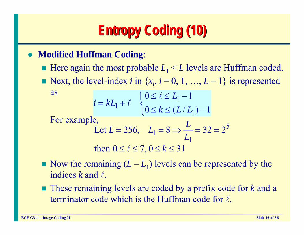
Entropy Coding (10)Entropy Coding (10)Modified Huffman Coding:
Here again the most probable L1 < L levels are Huffman coded.Next, the level-index i in {xi, i = 0, 1, …, L – 1} is represented as
For example,
Now the remaining (L – L1) levels can be represented by the indices k and l.These remaining levels are coded by a prefix code for k and a terminator code which is the Huffman code for l.
11
1
0 10 ( / ) 1
Li kL
k L L≤ ≤ −⎧
= + ⎨ ≤ ≤ −⎩
ll
51
1Let 256, 8 32 2
then 0 7, 0 31
LL LL
k
= = ⇒ = =
≤ ≤ ≤ ≤l
ECE G311 – Image Coding-II Slide 17 of 36
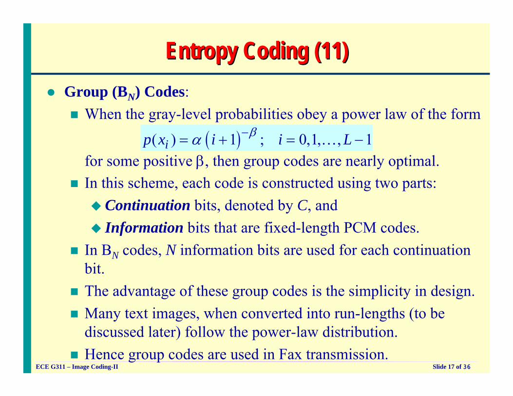
Entropy Coding (11)Entropy Coding (11)Group (BN) Codes:
When the gray-level probabilities obey a power law of the form
for some positive β, then group codes are nearly optimal.In this scheme, each code is constructed using two parts:
Continuation bits, denoted by C, and Information bits that are fixed-length PCM codes.
In BN codes, N information bits are used for each continuation bit.The advantage of these group codes is the simplicity in design.Many text images, when converted into run-lengths (to be discussed later) follow the power-law distribution.Hence group codes are used in Fax transmission.
( )( ) 1 ; 0,1, , 1ip x i i Lβα −= + = −K
ECE G311 – Image Coding-II Slide 18 of 36
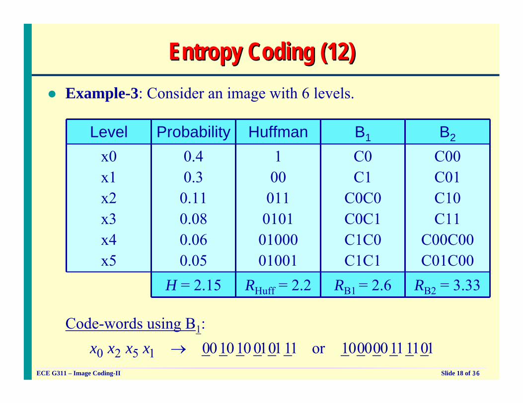
Entropy Coding (12)Entropy Coding (12)Example-3: Consider an image with 6 levels.
RB2 = 3.33RB1 = 2.6RHuff = 2.2H = 2.15
C00C01C10C11
C00C00C01C00
C0C1
C0C0C0C1C1C0C1C1
10001101010100001001
0.40.30.110.080.060.05
x0x1x2x3x4x5
B2B1HuffmanProbabilityLevel
Code-words using B1:
0 2 5 1 001010 010111 or 100000111101x x x x →
ECE G311 – Image Coding-II Slide 19 of 36
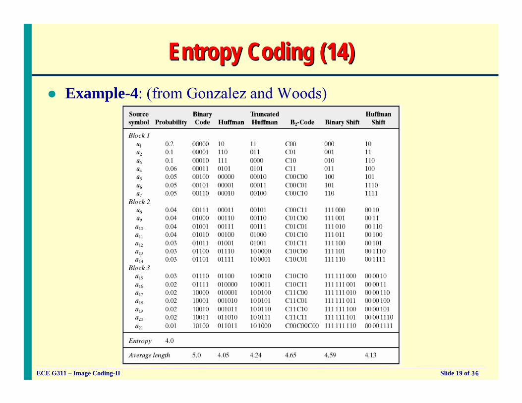
Entropy Coding (14)Entropy Coding (14)Example-4: (from Gonzalez and Woods)
ECE G311 – Image Coding-II Slide 20 of 36
Entropy Coding (16)Entropy Coding (16)Lempel-Ziv-Welch (LZW) Code: This coding scheme has gained a wide acceptance especially for computer files.
It is used in .zip, uuencode, uudecode, gzip, .tiff, etc. algorithms.The scheme uses variable-to-variable-length codes, in which both the number of source symbols encoded and the number of encoded bits per codeword are variable. Moreover, the code is space-varying.It does not require prior knowledge of the source statistics, yet over time it adapts so that the average codeword length R per source letter is minimized. Such algorithms are called universal Algorithms.
ECE G311 – Image Coding-II Slide 21 of 36
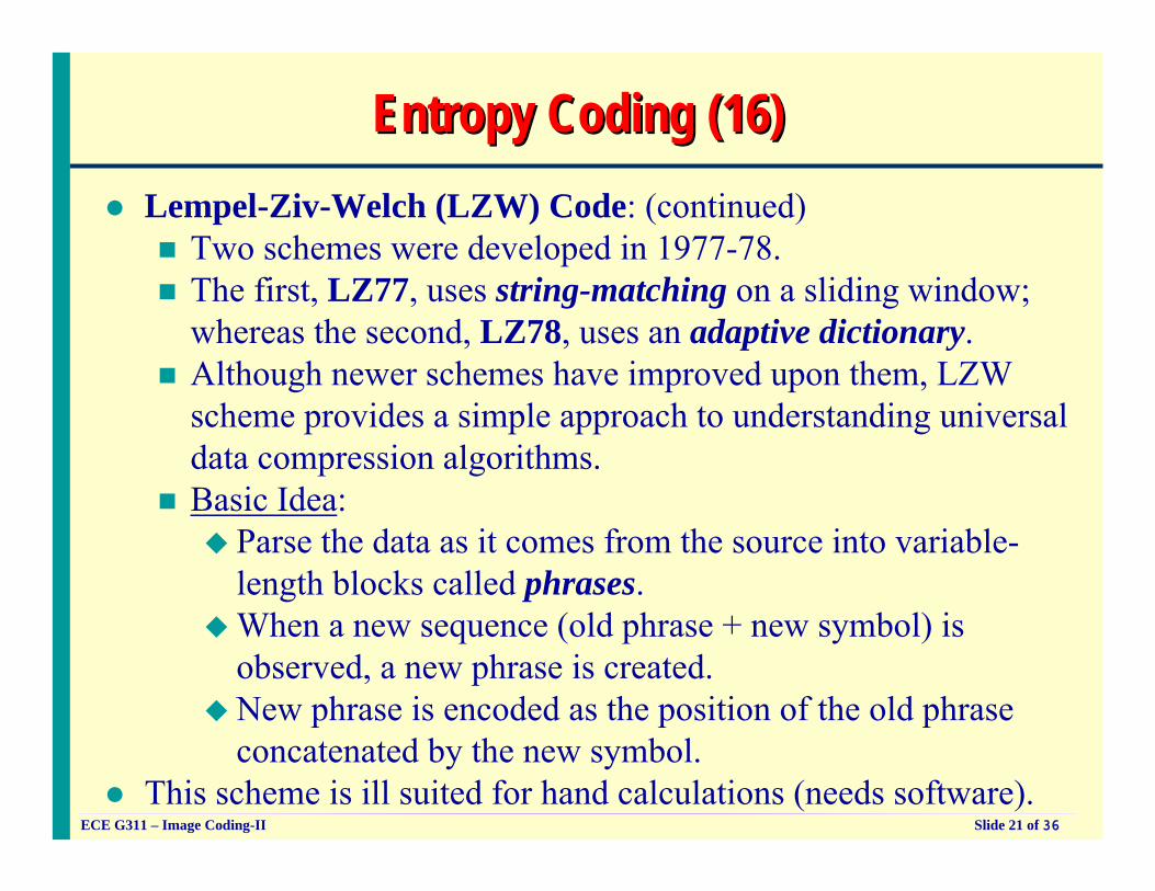
Entropy Coding (16)Entropy Coding (16)Lempel-Ziv-Welch (LZW) Code: (continued)
Two schemes were developed in 1977-78. The first, LZ77, uses string-matching on a sliding window; whereas the second, LZ78, uses an adaptive dictionary.Although newer schemes have improved upon them, LZW scheme provides a simple approach to understanding universal data compression algorithms.Basic Idea:
Parse the data as it comes from the source into variable-length blocks called phrases.When a new sequence (old phrase + new symbol) is observed, a new phrase is created.New phrase is encoded as the position of the old phrase concatenated by the new symbol.
This scheme is ill suited for hand calculations (needs software).
ECE G311 – Image Coding-II Slide 22 of 36
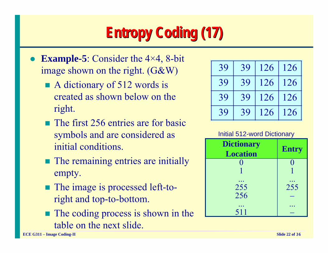
Entropy Coding (17)Entropy Coding (17)Example-5: Consider the 4×4, 8-bit image shown on the right. (G&W)
A dictionary of 512 words is created as shown below on the right.The first 256 entries are for basic symbols and are considered as initial conditions.The remaining entries are initially empty.The image is processed left-to-right and top-to-bottom.The coding process is shown in the table on the next slide.
39 39 126 12639 39 126 12639 39 126 12639 39 126 126
01...
255−...−
01...
255256...
511
EntryDictionary Location
Initial 512-word Dictionary
ECE G311 – Image Coding-II Slide 23 of 36
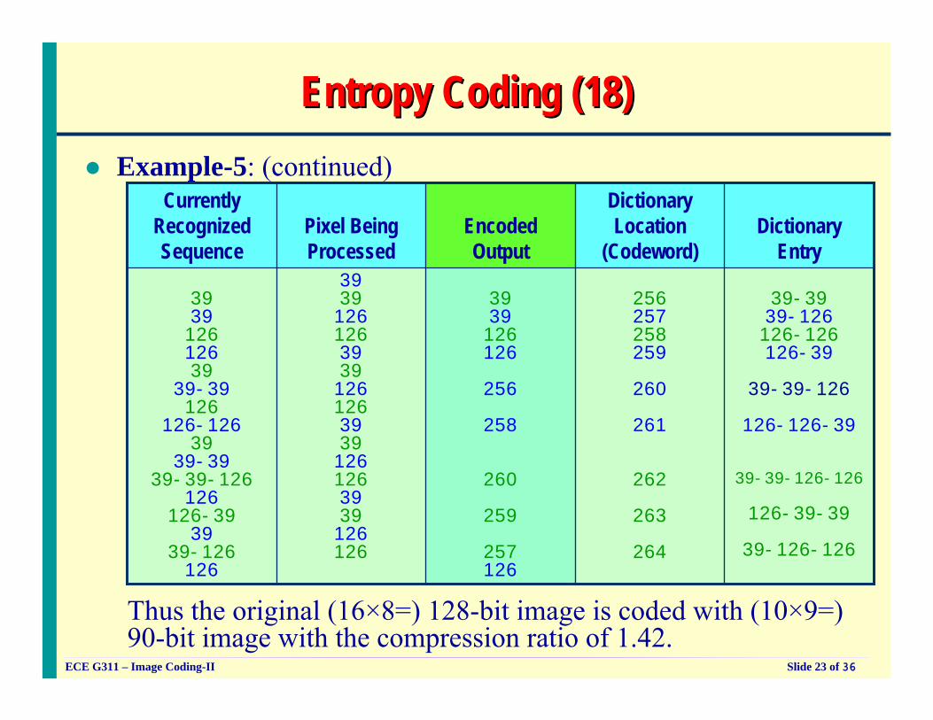
Entropy Coding (18)Entropy Coding (18)Example-5: (continued)
39-3939-126126-126126-39
39-39-126
126-126-39
39-39-126-126
126-39-39
39-126-126
256257258259
260
261
262
263
264
3939126126
256
258
260
259
257126
3939126126393912612639391261263939126126
393912612639
39-39126
126-12639
39-3939-39-126
126126-3939
39-126126
Dictionary Entry
Dictionary Location
(Codeword)Encoded Output
Pixel Being Processed
Currently Recognized Sequence
Thus the original (16×8=) 128-bit image is coded with (10×9=) 90-bit image with the compression ratio of 1.42.
ECE G311 – Image Coding-II Slide 24 of 36
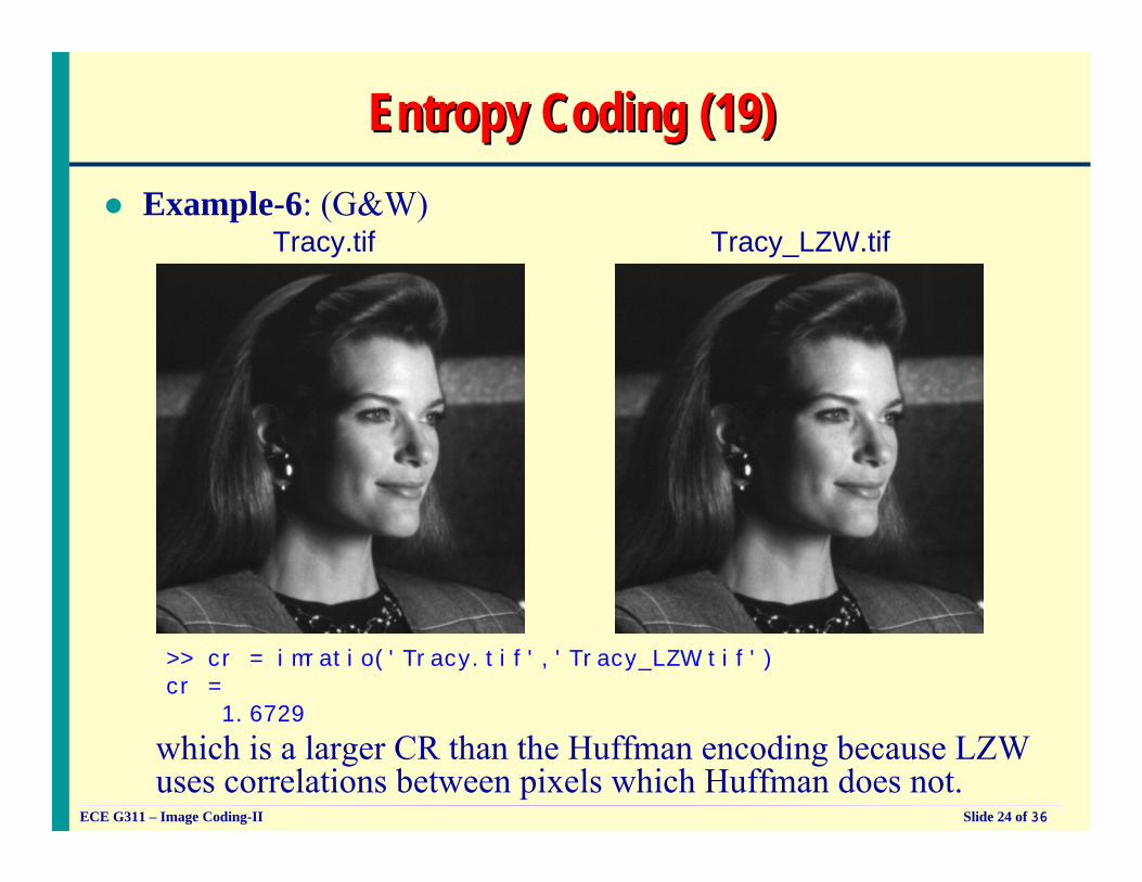
Entropy Coding (19)Entropy Coding (19)
Tracy.tif Tracy_LZW.tif
>> cr = imratio('Tracy.tif','Tracy_LZW.tif')cr =
1.6729
which is a larger CR than the Huffman encoding because LZW uses correlations between pixels which Huffman does not.
Example-6: (G&W)
ECE G311 – Image Coding-II Slide 25 of 36
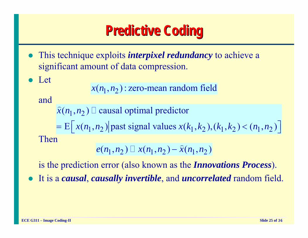
Predictive CodingPredictive CodingThis technique exploits interpixel redundancy to achieve a significant amount of data compression.Let
and
Then
is the prediction error (also known as the Innovations Process).It is a causal, causally invertible, and uncorrelated random field.
1 2( , ) : zero-mean random fieldx n n
1 2
1 2 1 2 1 2 1 2
( , ) causal optimal predictor
E ( , ) past signal values ( , ), ( , ) ( , )
x n n
x n n x k k k k n n⎡ ⎤= <⎣ ⎦
)
1 2 1 2 1 2( , ) ( , ) ( , )e n n x n n x n n− )
ECE G311 – Image Coding-II Slide 26 of 36
Predictive Coding (2)Predictive Coding (2)Basic Principle:Remove the mutual redundancy between successive pixels by quantizing and coding only the new information contained in the innovations process or in the error difference image.In general, the optimal predictor (conditional mean) is a nonlinear function of the past pixel values.However, in the case of a Gaussian random field, the optimal estimator is also linear which is easier to implement.For ease of implementation, we will consider only linear (and hence suboptimum) predictors.In this case, the prediction error is still causal, causally invertible, but is not uncorrelated (or white).
ECE G311 – Image Coding-II Slide 27 of 36
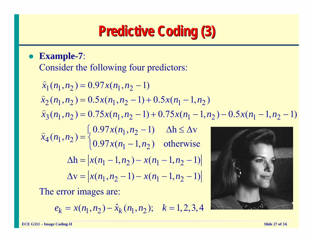
Predictive Coding (3)Predictive Coding (3)Example-7:Consider the following four predictors:
The error images are:
1 1 2 1 2
2 1 2 1 2 1 2
3 1 2 1 2 1 2 1 2
1 24 1 2
1 2
1 2 1 2
( , ) 0.97 ( , 1)( , ) 0.5 ( , 1) 0.5 ( 1, )( , ) 0.75 ( , 1) 0.75 ( 1, ) 0.5 ( 1, 1)
0.97 ( , 1) h v( , )
0.97 ( 1, ) otherwise
h ( 1, ) ( 1, 1
x n n x n nx n n x n n x n nx n n x n n x n n x n n
x n nx n n
x n n
x n n x n n
= −= − + −= − + − − − −
− Δ ≤ Δ⎧= ⎨ −⎩
Δ = − − − −
)
)
)
)
1 2 1 2
)
v ( , 1) ( 1, 1)x n n x n nΔ = − − − −
1 2 1 2ˆ( , ) ( , ); 1, 2,3,4k ke x n n x n n k= − =
ECE G311 – Image Coding-II Slide 28 of 36
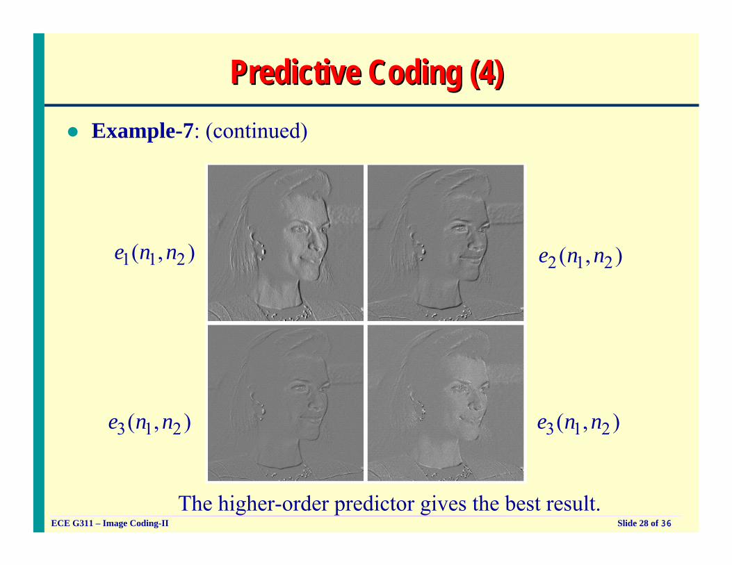
Predictive Coding (4)Predictive Coding (4)Example-7: (continued)
The higher-order predictor gives the best result.
1 1 2( , )e n n 2 1 2( , )e n n
3 1 2( , )e n n 3 1 2( , )e n n
ECE G311 – Image Coding-II Slide 29 of 36
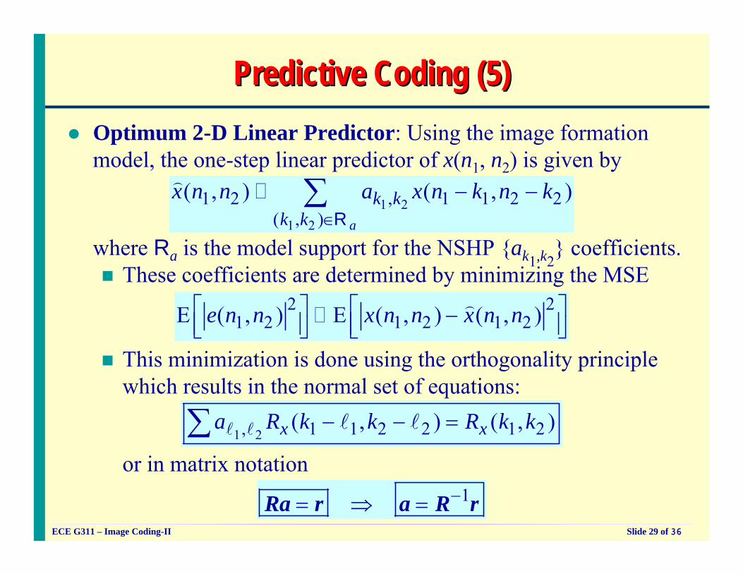
Predictive Coding (5)Predictive Coding (5)Optimum 2-D Linear Predictor: Using the image formation model, the one-step linear predictor of x(n1, n2) is given by
1 21 2
1 2 , 1 1 2 2( , )
( , ) ( , )a
k kk k
x n n a x n k n k∈
− −∑R
)
where Ra is the model support for the NSHP {ak1,k2} coefficients.
These coefficients are determined by minimizing the MSE
This minimization is done using the orthogonality principle which results in the normal set of equations:
2 21 2 1 2 1 2E ( , ) E ( , ) ( , )e n n x n n x n n⎡ ⎤ ⎡ ⎤−⎢ ⎥ ⎢ ⎥⎣ ⎦ ⎣ ⎦
)
or in matrix notation1 2, 1 1 2 2 1 2( , ) ( , )x xa R k k R k k− − =∑ l l l l
1−= ⇒ =Ra r a R r
ECE G311 – Image Coding-II Slide 30 of 36
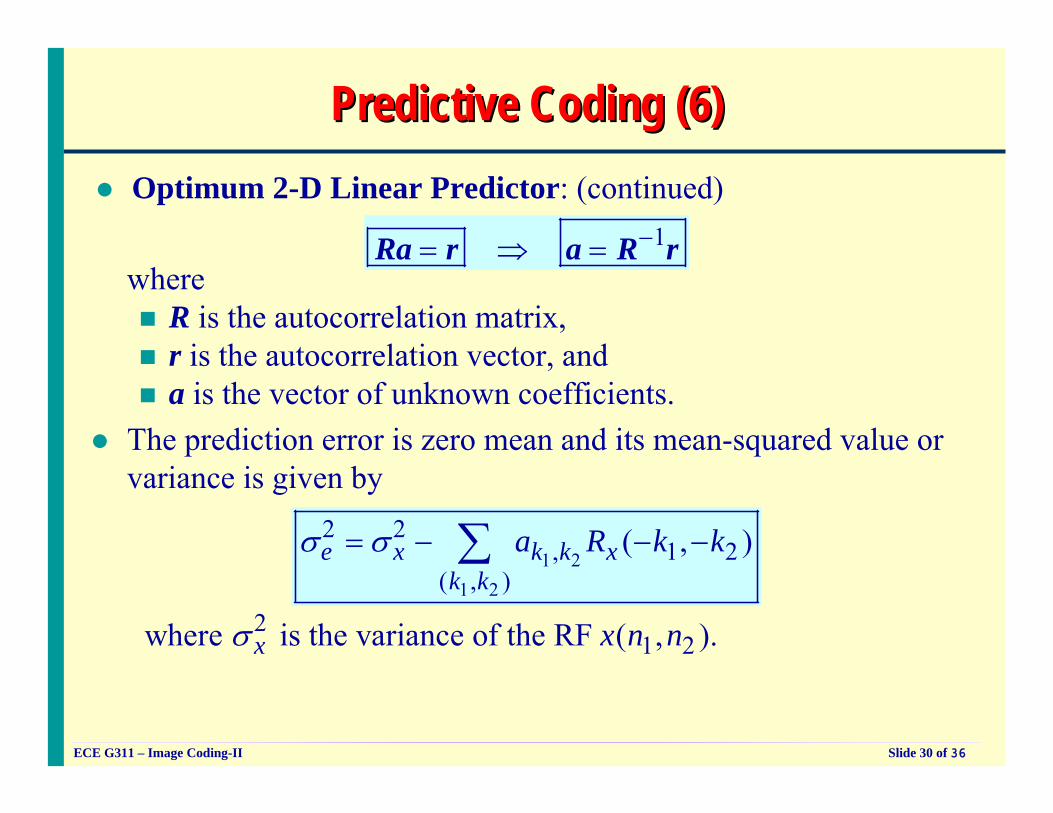
Predictive Coding (6)Predictive Coding (6)Optimum 2-D Linear Predictor: (continued)
1−= ⇒ =Ra r a R rwhere
R is the autocorrelation matrix, r is the autocorrelation vector, and a is the vector of unknown coefficients.
The prediction error is zero mean and its mean-squared value or variance is given by
1 21 2
2 2, 1 2
( , )( , )e x k k x
k ka R k kσ σ= − − −∑
21 2 where is the variance of the RF ( , ).x x n nσ
ECE G311 – Image Coding-II Slide 31 of 36
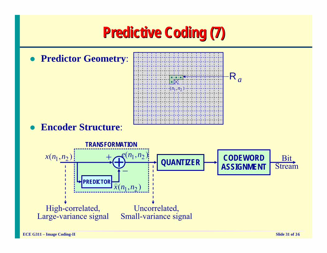
Predictive Coding (7)Predictive Coding (7)Predictor Geometry:
1 2( , )n naR
Encoder Structure:
TRANSFORMATION
QUANTIZER CODEWORDASSIGNMENT
1 2( , )x n n BitStream
1 2( , )e n n
PREDICTOR1 2( , )x n n)
Uncorrelated,Small-variance signal
High-correlated,Large-variance signal
+−
ECE G311 – Image Coding-II Slide 32 of 36
Predictive Coding (8)Predictive Coding (8)Linear Predictive Coding (LPC) Techniques:Based on the complexity in the predictor and the quantizer, we have three approaches:
Delta Modulation (DM):Uses a 1st-order one-step predictor and one bit in the quantizer.Differential Pulse Code Modulation (DPCM):Uses higher-order predictors and more bits in the quantizer. There are two possibilities:
Line-by-Line DPCM:This approach predicts one entire scan-line using a 1-D vector predictor.2-D DPCM:This approach predicts one pixel at a time using 2-D scalar predictor.
ECE G311 – Image Coding-II Slide 33 of 36
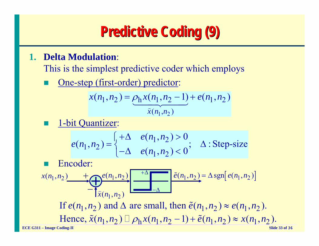
Predictive Coding (9)Predictive Coding (9)1. Delta Modulation:
This is the simplest predictive coder which employsOne-step (first-order) predictor:
1-bit Quantizer:
Encoder:
1 2
1 2 h 1 2 1 2( , )
( , ) ( , 1) ( , )x n n
x n n x n n e n nρ= − +)
1442443
1 21 2
1 2
( , ) 0( , ) ; : Step-size
( , ) 0e n n
e n ne n n
+Δ >⎧= Δ⎨−Δ <⎩
1 2( , )x n n 1 2( , )e n n
1 2( , )x n n)
+−
+Δ
−Δ
[ ]1 2 1 2( , ) sgn ( , )e n n e n n= Δ%
1 2 1 2 1 2
1 2 h 1 2 1 2 1 2
If ( , ) and are small, then ( , ) ( , ).Hence, ( , ) ( , 1) ( , ) ( , ).
e n n e n n e n nx n n x n n e n n x n nρ
Δ ≈− + ≈
%
% %
ECE G311 – Image Coding-II Slide 34 of 36
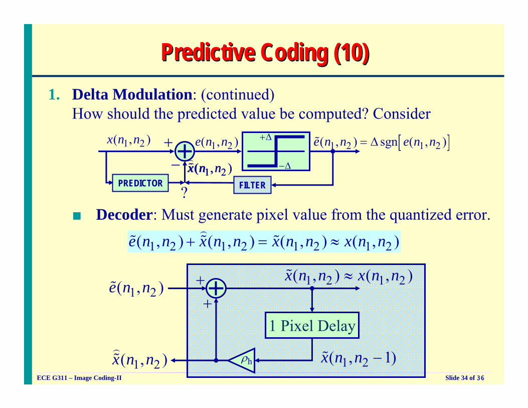
Predictive Coding (10)Predictive Coding (10)1. Delta Modulation: (continued)
How should the predicted value be computed? Consider
1 2( , )x n n 1 2( , )e n n
1 2( , )x n n)
+−
+Δ
−Δ
[ ]1 2 1 2( , ) sgn ( , )e n n e n n= Δ%
?PREDICTOR FILTER
■ Decoder: Must generate pixel value from the quantized error.
1 2 1 2 1 2 1 2( , ) ( , ) ( , ) ( , )e n n x n n x n n x n n+ = ≈)
% % %
1 Pixel Delay
hρ
1 2( , )e n n% 1 2( , )x n n%
1 2( , )x n n)%
++
1 2( , )x n n≈
1 2( , )x n n)%
1 2( , 1)x n n −%
ECE G311 – Image Coding-II Slide 35 of 36
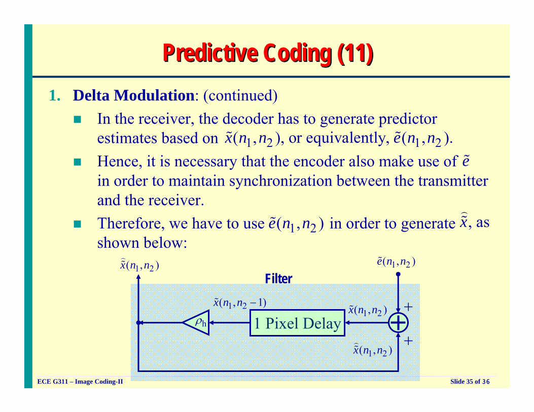
Predictive Coding (11)Predictive Coding (11)1. Delta Modulation: (continued)
In the receiver, the decoder has to generate predictor estimates based on Hence, it is necessary that the encoder also make use of in order to maintain synchronization between the transmitter and the receiver.Therefore, we have to use in order to generateshown below:
1 2 1 2( , ), or equivalently, ( , ).x n n e n n% %
e%
1 2( , )e n n% , asx)%
1 Pixel Delayhρ
1 2( , )e n n%
1 2( , )x n n%
1 2( , )x n n)%
+
+
1 2( , 1)x n n −%
1 2( , )x n n)%
Filter
ECE G311 – Image Coding-II Slide 36 of 36
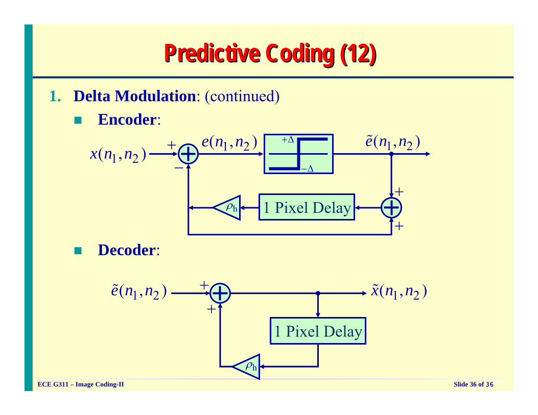
Predictive Coding (12)Predictive Coding (12)1. Delta Modulation: (continued)
Encoder:
1 2( , )x n n 1 2( , )e n n+−
+Δ
−Δ
Decoder:
1 Pixel Delay
hρ
1 2( , )e n n% 1 2( , )x n n%++
1 Pixel Delayhρ
1 2( , )e n n%
+
+
ECE G311 – Image Coding-II Slide 37 of 36
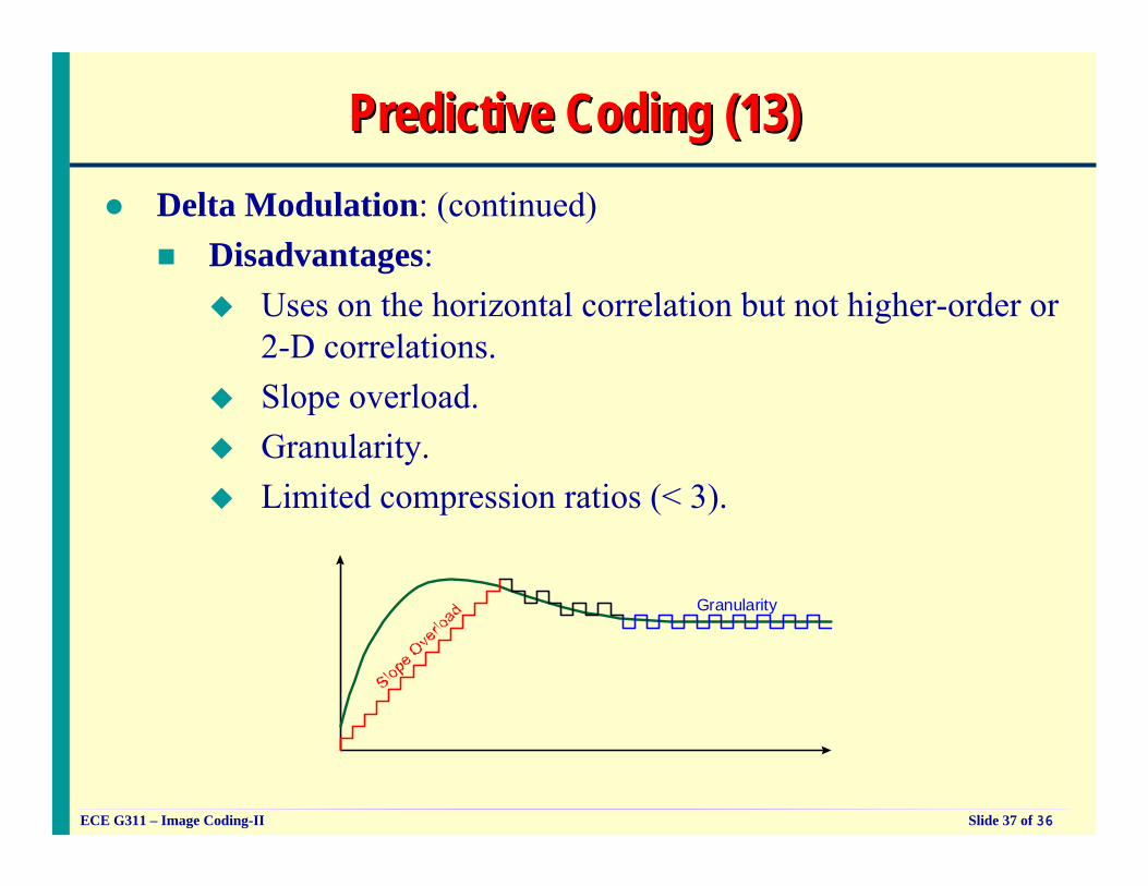
Predictive Coding (13)Predictive Coding (13)Delta Modulation: (continued)
Disadvantages:Uses on the horizontal correlation but not higher-order or 2-D correlations.Slope overload.Granularity.Limited compression ratios (< 3).
Granularity
ECE G311 – Image Coding-II Slide 38 of 36
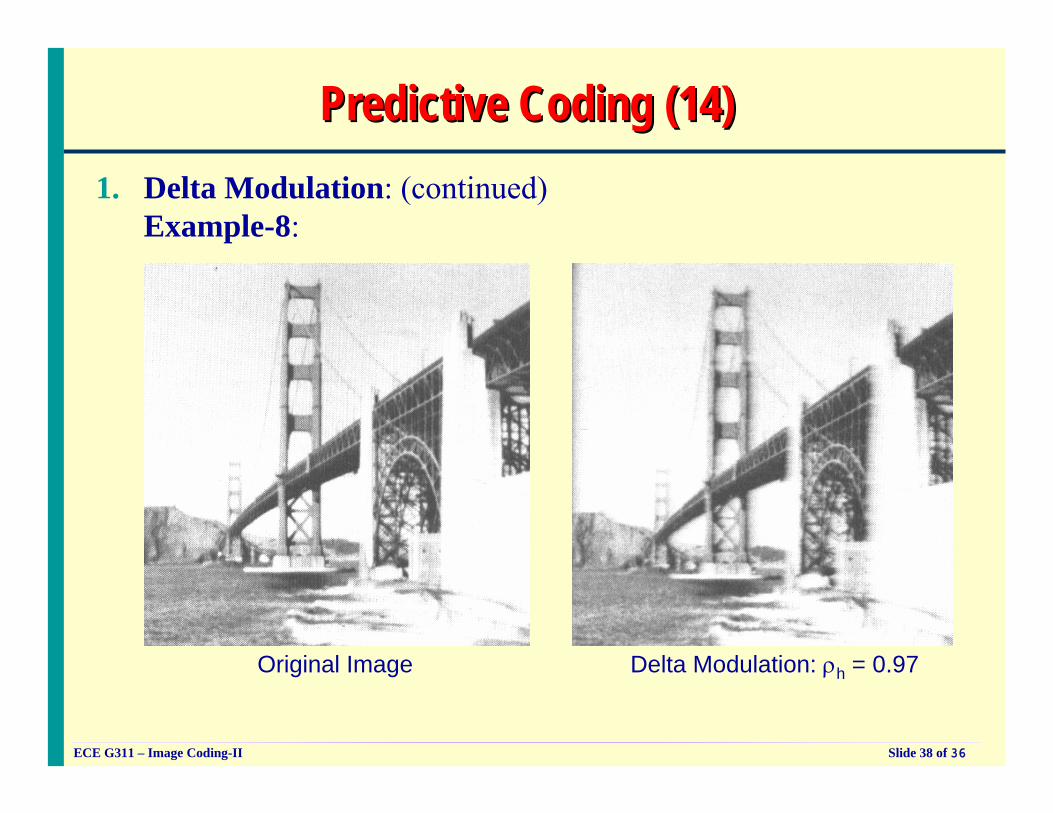
Predictive Coding (14)Predictive Coding (14)1. Delta Modulation: (continued)
Example-8:
Original Image Delta Modulation: ρh = 0.97
ECE G311 – Image Coding-II Slide 39 of 36
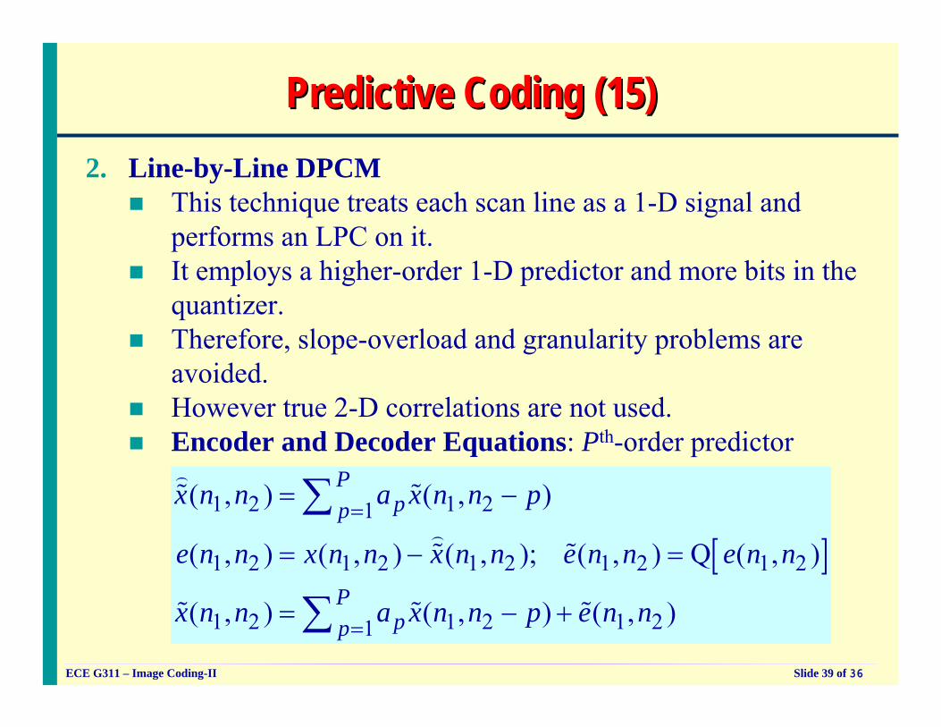
Predictive Coding (15)Predictive Coding (15)2. Line-by-Line DPCM
This technique treats each scan line as a 1-D signal and performs an LPC on it.It employs a higher-order 1-D predictor and more bits in the quantizer. Therefore, slope-overload and granularity problems are avoided.However true 2-D correlations are not used.Encoder and Decoder Equations: Pth-order predictor
[ ]1 2 1 21
1 2 1 2 1 2 1 2 1 2
1 2 1 2 1 21
( , ) ( , )
( , ) ( , ) ( , ); ( , ) Q ( , )
( , ) ( , ) ( , )
Ppp
Ppp
x n n a x n n p
e n n x n n x n n e n n e n n
x n n a x n n p e n n
=
=
= −
= − =
= − +
∑
∑
)% %
)% %
% % %
ECE G311 – Image Coding-II Slide 40 of 36
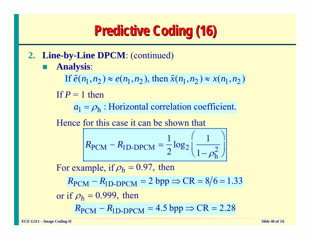
Predictive Coding (16)Predictive Coding (16)2. Line-by-Line DPCM: (continued)
Analysis:
If P = 1 then
Hence for this case it can be shown that
For example, if
or if
1 2 1 2 1 2 1 2If ( , ) ( , ), then ( , ) ( , )e n n e n n x n n x n n≈ ≈% %
1 h : Horizontal correlation coefficient.a ρ=
PCM 1D-DPCM 2 2h
1 1log2 1
R Rρ
⎛ ⎞− = ⎜ ⎟
−⎝ ⎠0.97, thenhρ =
PCM 1D-DPCM 2 bpp CR 8 6 1.33R R− = ⇒ = =
0.999, thenhρ =
PCM 1D-DPCM 4.5 bpp CR 2.28R R− = ⇒ =
ECE G311 – Image Coding-II Slide 41 of 36
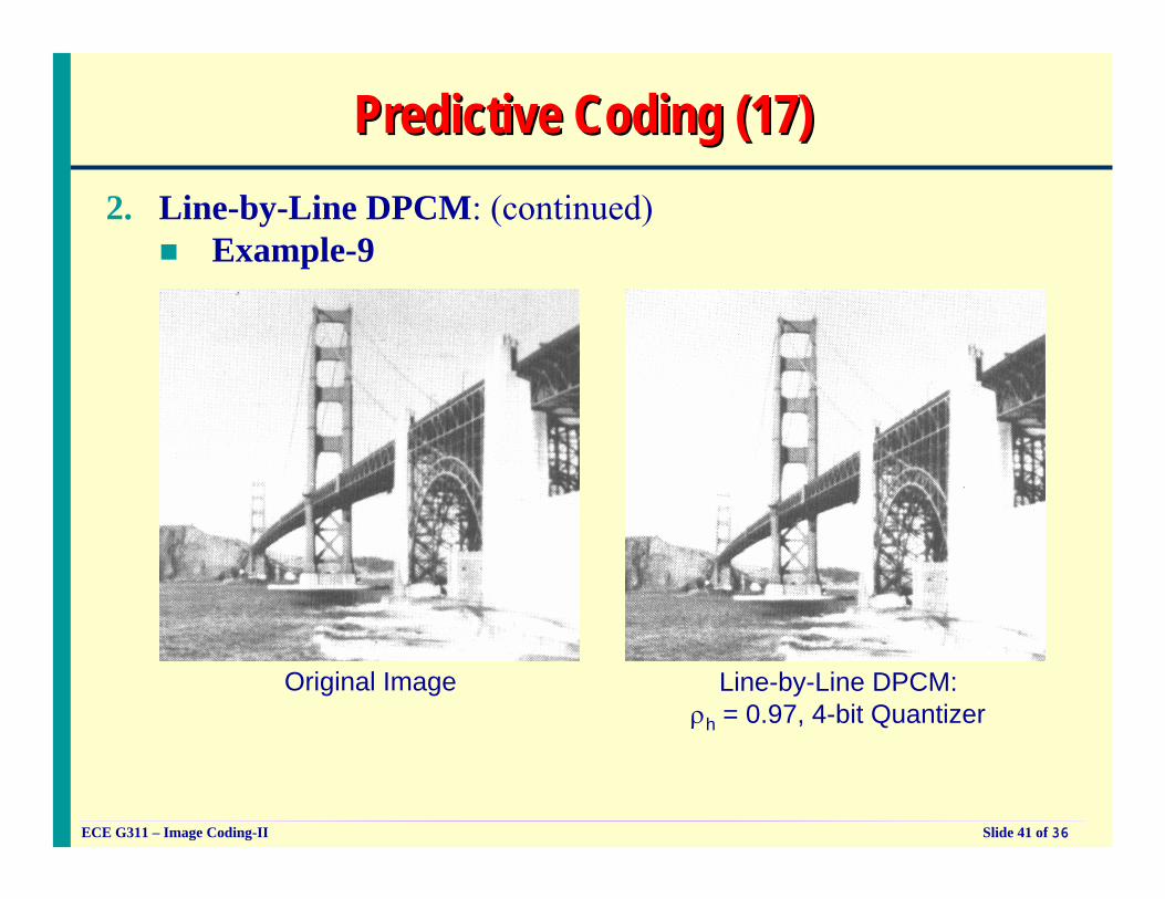
Predictive Coding (17)Predictive Coding (17)2. Line-by-Line DPCM: (continued)
Example-9
Original Image Line-by-Line DPCM: ρh = 0.97, 4-bit Quantizer
ECE G311 – Image Coding-II Slide 42 of 36
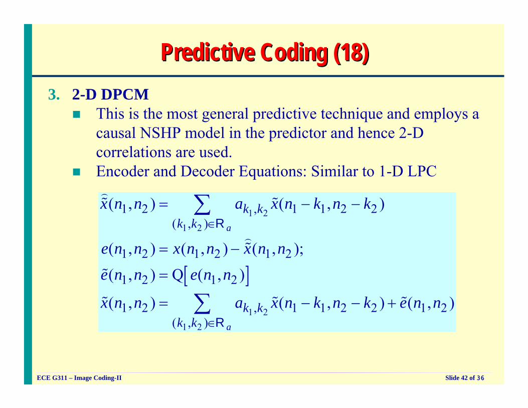
Predictive Coding (18)Predictive Coding (18)3. 2-D DPCM
This is the most general predictive technique and employs a causal NSHP model in the predictor and hence 2-D correlations are used.Encoder and Decoder Equations: Similar to 1-D LPC
[ ]
1 21 2
1 21 2
1 2 , 1 1 2 2( , )
1 2 1 2 1 2
1 2 1 2
1 2 , 1 1 2 2 1 2( , )
( , ) ( , )
( , ) ( , ) ( , );( , ) Q ( , )
( , ) ( , ) ( , )
a
a
k kk k
k kk k
x n n a x n k n k
e n n x n n x n ne n n e n n
x n n a x n k n k e n n
∈
∈
= − −
= −
=
= − − +
∑
∑
R
R
)% %
)%
%
% % %
ECE G311 – Image Coding-II Slide 43 of 36
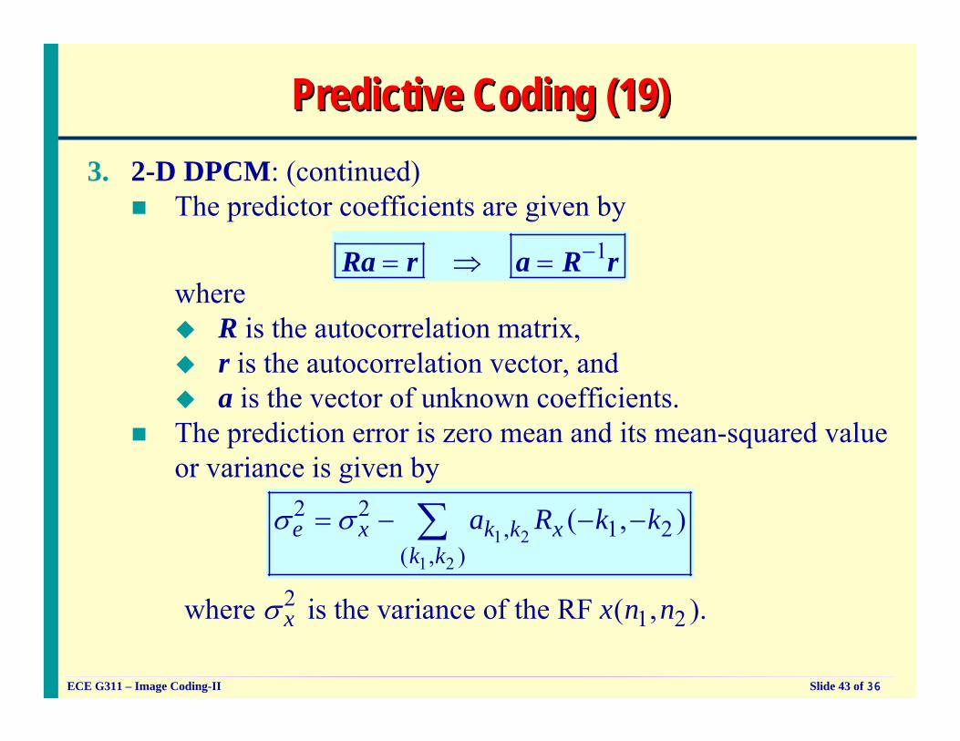
Predictive Coding (19)Predictive Coding (19)3. 2-D DPCM: (continued)
The predictor coefficients are given by
where R is the autocorrelation matrix, r is the autocorrelation vector, and a is the vector of unknown coefficients.
The prediction error is zero mean and its mean-squared value or variance is given by
1−= ⇒ =Ra r a R r
1 21 2
2 2, 1 2
( , )( , )e x k k x
k ka R k kσ σ= − − −∑
21 2 where is the variance of the RF ( , ).x x n nσ
ECE G311 – Image Coding-II Slide 44 of 36
( ) ( )2 2v h2
v h 2(1,0) (0,1)
(1,1)(0,0)
x x x xx x
xx
R RR
R
σ ρ σ ρσ ρ ρ
σ= = =
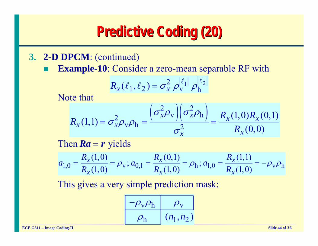
Predictive Coding (20)Predictive Coding (20)3. 2-D DPCM: (continued)
Example-10: Consider a zero-mean separable RF with
Note that
Then
This gives a very simple prediction mask:
2121 2 v h( , )x xR σ ρ ρ= lll l
yields=Ra r
1,0 v 0,1 h 1,0 v h(1,0) (0,1) (1,1)
; ;(1,0) (1,0) (1,0)
x x x
x x x
R R Ra a a
R R Rρ ρ ρ ρ= = = = = = −
v h v
h 1 2( , )n nρ ρ ρρ
−
ECE G311 – Image Coding-II Slide 45 of 36
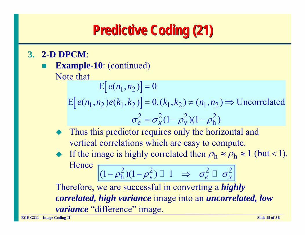
Predictive Coding (21)Predictive Coding (21)3. 2-D DPCM:
Example-10: (continued)Note that
Thus this predictor requires only the horizontal and vertical correlations which are easy to compute.If the image is highly correlated thenHence
Therefore, we are successful in converting a highly correlated, high variance image into an uncorrelated, low variance “difference” image.
[ ][ ]
1 2
1 2 1 2 1 2 1 22 2 2 2
v h
E ( , ) 0
E ( , ) ( , ) 0,( , ) ( , ) Uncorrelated
(1 )(1 )e x
e n n
e n n e k k k k n n
σ σ ρ ρ
=
= ≠ ⇒
= − −
h h 1 (but 1).ρ ρ≈ ≈ <
2 2 2 2h v(1 )(1 ) 1 e xρ ρ σ σ− − ⇒
ECE G311 – Image Coding-II Slide 46 of 36
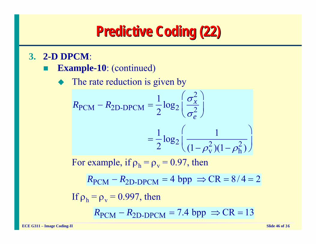
Predictive Coding (22)Predictive Coding (22)3. 2-D DPCM:
Example-10: (continued)The rate reduction is given by
For example, if ρh = ρv = 0.97, then
If ρh = ρv = 0.997, then
2
PCM 2D-DPCM 2 2
2 2 2v h
1 log2
1 1log2 (1 )(1 )
x
eR R
σσ
ρ ρ
⎛ ⎞− = ⎜ ⎟
⎝ ⎠
⎛ ⎞= ⎜ ⎟
− −⎝ ⎠
PCM 2D-DPCM 4 bpp CR 8/ 4 2R R− = ⇒ = =
PCM 2D-DPCM 7.4 bpp CR 13R R− = ⇒ =
ECE G311 – Image Coding-II Slide 47 of 36
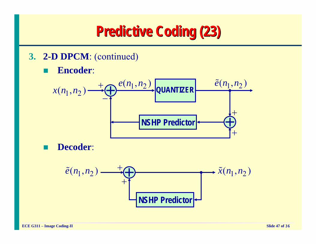
Predictive Coding (23)Predictive Coding (23)3. 2-D DPCM: (continued)
Encoder:
1 2( , )x n n 1 2( , )e n n+−
NSHP Predictor
1 2( , )e n n%
+
+
Decoder:
1 2( , )e n n% 1 2( , )x n n%++
QUANTIZER
NSHP Predictor
ECE G311 – Image Coding-II Slide 48 of 36
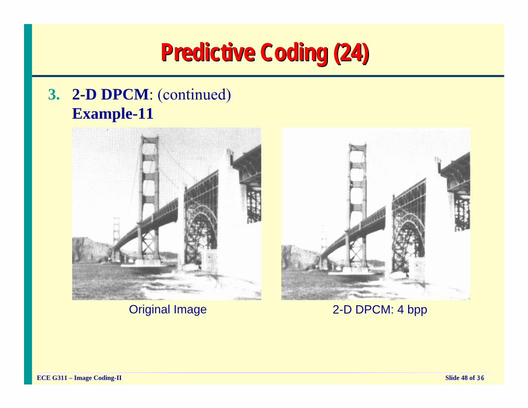
Predictive Coding (24)Predictive Coding (24)3. 2-D DPCM: (continued)
Example-11
Original Image 2-D DPCM: 4 bpp
ECE G311 – Image Coding-II Slide 49 of 36
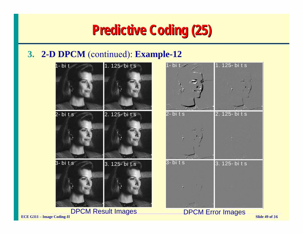
Predictive Coding (25)Predictive Coding (25)
DPCM Result Images DPCM Error Images
1-bit 1.125-bits
2.125-bits
3.125-bits
2-bits
3-bits
1-bit 1.125-bits
2.125-bits
3.125-bits
2-bits
3-bits
3. 2-D DPCM (continued): Example-12
ECE G311 – Image Coding-II Slide 50 of 36
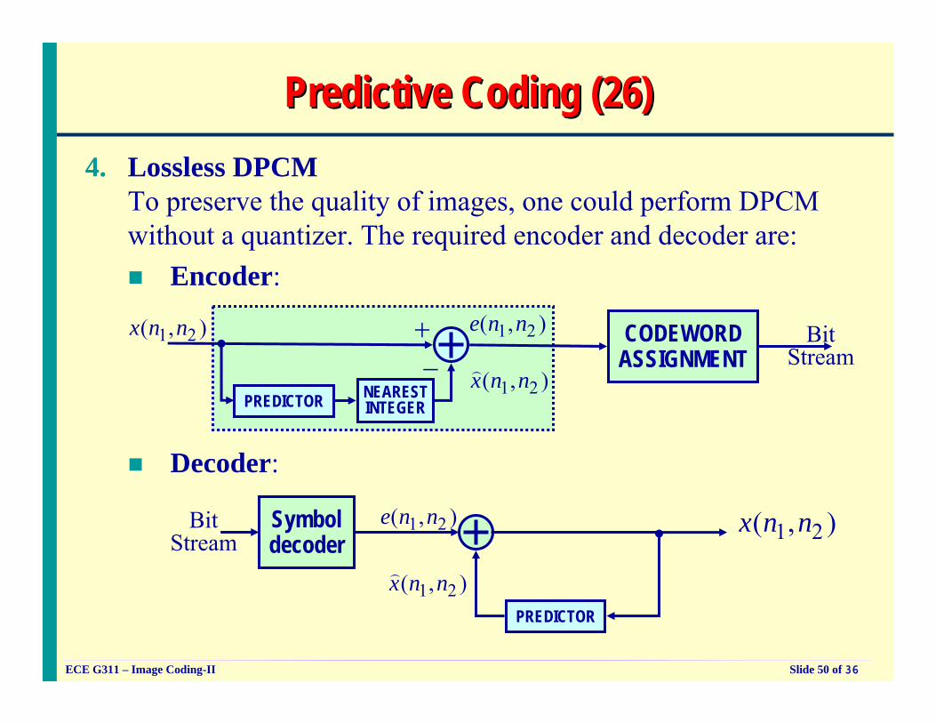
Predictive Coding (26)Predictive Coding (26)4. Lossless DPCM
To preserve the quality of images, one could perform DPCM without a quantizer. The required encoder and decoder are:
Encoder:
Decoder:
BitStream
CODEWORDASSIGNMENT
1 2( , )x n n 1 2( , )e n n
PREDICTOR1 2( , )x n n)
+−
NEARESTINTEGER
1 2( , )e n n1 2( , )x n nSymbol
decoder
PREDICTOR1 2( , )x n n)
BitStream
ECE G311 – Image Coding-II Slide 51 of 36
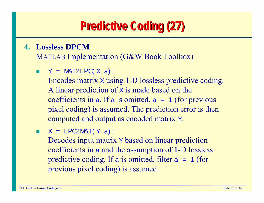
Predictive Coding (27)Predictive Coding (27)4. Lossless DPCM
MATLAB Implementation (G&W Book Toolbox)
Y = MAT2LPC(X,a);
Encodes matrix X using 1-D lossless predictive coding. A linear prediction of X is made based on the coefficients in a. If a is omitted, a = 1 (for previous pixel coding) is assumed. The prediction error is then computed and output as encoded matrix Y.X = LPC2MAT(Y,a);
Decodes input matrix Y based on linear prediction coefficients in a and the assumption of 1-D lossless predictive coding. If a is omitted, filter a = 1 (for previous pixel coding) is assumed.
ECE G311 – Image Coding-II Slide 52 of 36
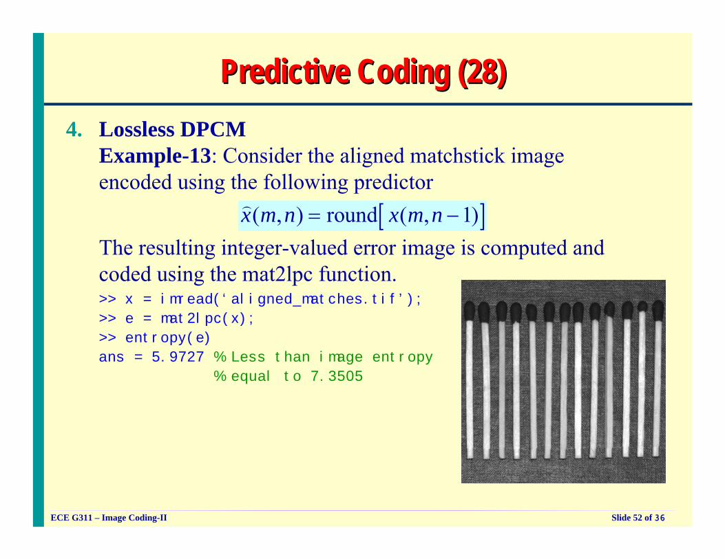
Predictive Coding (28)Predictive Coding (28)4. Lossless DPCM
Example-13: Consider the aligned matchstick image encoded using the following predictor
The resulting integer-valued error image is computed and coded using the mat2lpc function.
[ ]( , ) round ( , 1)x m n x m n= −)
>> x = imread(‘aligned_matches.tif’);
>> e = mat2lpc(x);
>> entropy(e)
ans = 5.9727 % Less than image entropy
% equal to 7.3505
ECE G311 – Image Coding-II Slide 53 of 36
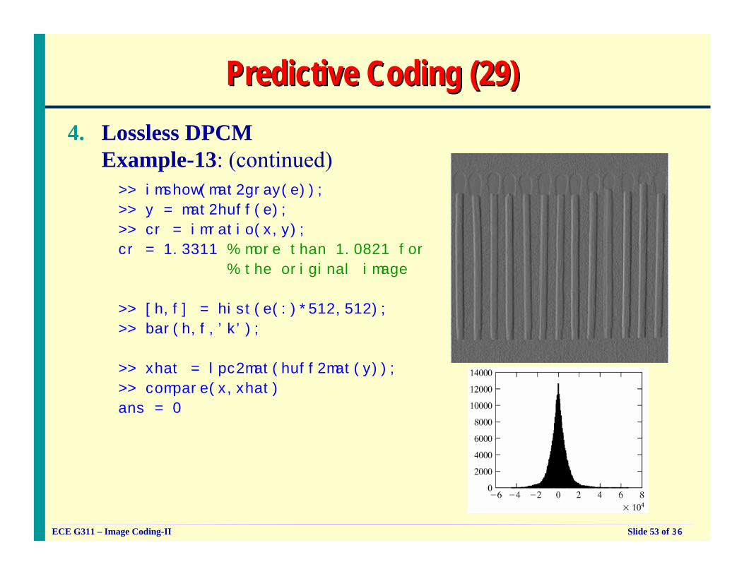
Predictive Coding (29)Predictive Coding (29)4. Lossless DPCM
Example-13: (continued)>> imshow(mat2gray(e));
>> y = mat2huff(e);
>> cr = imratio(x,y);
cr = 1.3311 % more than 1.0821 for
% the original image
>> [h,f] = hist(e(:)*512,512);
>> bar(h,f,’k’);
>> xhat = lpc2mat(huff2mat(y));
>> compare(x,xhat)
ans = 0