![Arthritis Research UK Epidemiology Unit University of ...personalpages.manchester.ac.uk/staff/mark.lunt/stats/11_Stata_2/...Other Graph Types twoway lfit[ci] Linear regression fit](https://static.fdocuments.us/doc/165x107/5aafdfdb7f8b9a22118dc053/arthritis-research-uk-epidemiology-unit-university-of-graph-types-twoway-lfitci.jpg)
TOPIC E: OSCILLATIONS SPRING 2018 - University of...
22
Mechanics Topic E (Oscillations) - 1 David Apsley TOPIC E: OSCILLATIONS SPRING 2018 1. Introduction 1.1 Overview 1.2 Degrees of freedom 1.3 Simple harmonic motion 2. Undamped free oscillation 2.1 Generalised mass-spring system: simple harmonic motion 2.2 Natural frequency and period 2.3 Amplitude and phase 2.4 Velocity and acceleration 2.5 Displacement from equilibrium 2.6 Small-amplitude approximations 2.7 Derivation of the SHM equation from energy principles 3. Damped free oscillation 3.1 The equation of motion 3.2 Solution for different damping levels 4. Forced oscillation 4.1 Mathematical expression of the problem 4.2 Static load 4.3 Undamped forced oscillation 4.4 Damped forced oscillation
Transcript of TOPIC E: OSCILLATIONS SPRING 2018 - University of...

Mechanics Topic E (Oscillations) - 1 David Apsley
TOPIC E: OSCILLATIONS SPRING 2018
1. Introduction
1.1 Overview
1.2 Degrees of freedom
1.3 Simple harmonic motion
2. Undamped free oscillation
2.1 Generalised mass-spring system: simple harmonic motion
2.2 Natural frequency and period
2.3 Amplitude and phase
2.4 Velocity and acceleration
2.5 Displacement from equilibrium
2.6 Small-amplitude approximations
2.7 Derivation of the SHM equation from energy principles
3. Damped free oscillation
3.1 The equation of motion
3.2 Solution for different damping levels
4. Forced oscillation
4.1 Mathematical expression of the problem
4.2 Static load
4.3 Undamped forced oscillation
4.4 Damped forced oscillation

Mechanics Topic E (Oscillations) - 2 David Apsley
1. INTRODUCTION
1.1 Overview
Many important dynamical problems arise from the oscillation of systems responding to
applied disturbances in the presence of restoring forces. Examples include:
response of a structure to earthquakes;
human-induced structural oscillations (e.g. grandstands at concerts/sports venues);
flow-induced oscillations (e.g. chimneys, pipelines, power lines);
vibration of unbalanced rotating machinery.
Most systems when displaced from a position of equilibrium have one or more natural
frequencies of oscillation which depend upon the strength of restoring forces (stiffness) and
resistance to change of motion (inertia). If the system is left to oscillate without further
influence from outside this is referred to as free oscillation.
On the other hand, the examples above are mainly concerned with forced oscillation; that is,
oscillations of a certain frequency are imposed on the system by external forces. If the
applied frequency is close to the natural frequency of the system then there is considerable
transfer of energy and resonance occurs, with potentially catastrophic consequences.
In general, all systems are subject to some degree of frictional damping that removes energy.
A freely-oscillating system may be under-damped (oscillates, but with gradually diminishing
amplitude) or over-damped (so restricted that it never oscillates). When periodic forces act on
structures, damping is a crucial factor in reducing the amplitude of oscillation.
1.2 Degrees of Freedom Many systems have several modes of oscillation. For example, a long power line or
suspended bridge deck may “gallop” (bounce up and down) or it may twist. Often the
geometric configuration at any instant can be defined by a small number of parameters:
usually displacements x or angles θ. Parameters which are just sufficient to describe the
geometric configuration of the system are called degrees of freedom. Here, for simplicity, we
shall restrict ourselves to single-degree-of-freedom (SDOF) systems. The equation of motion
then describes the variation of that parameter with time.
Examples of SDOF dynamical systems and their degree of freedom are:
mass suspended by a spring (vertical displacement);
pivoted body (angular displacement).
In both systems, oscillations occur about a position of static equilibrium in which applied
forces or moments are in balance.
1.3 Simple Harmonic Motion
For many systems the forces arising from a small displacement are opposite in direction and
proportional in size to the displacement. The equation of motion is particularly simple and
solutions take the form of a sinusoidal variation with time. This ubiquitous and important
type of oscillation is known as simple harmonic motion (SHM).

Mechanics Topic E (Oscillations) - 3 David Apsley
2. UNDAMPED FREE OSCILLATION The oscillatory motion of a system displaced from stable equilibrium and then allowed to
adjust in the absence of externally-imposed forces is termed free oscillation. If there are no
frictional forces the motion is called undamped free oscillation.
2.1 Generalised Mass-Spring System: Simple Harmonic Motion This is a general model for a linear free-oscillation problem. It doesn’t physically have to
correspond to masses and springs.
A generalised mass-spring system is one for which the resultant
force following displacement from equilibrium is a function of the
displacement and of opposite sign (i.e. a restoring force). For ideal
springs (or, in practice, for small displacements) the relationship is
linear:
kxFx (1)
k is called the stiffness or spring constant. It is measured in newtons per metre (N m–1
). The
equation of motion is then
kxt
xm
2
2
d
d (2)
To solve (2) note that xmktx )/(/dd 22 and that k/m is a positive constant. Thus, it is
common to write the equation as
Simple Harmonic Motion (SHM) Equation:
xt
x 2
2
2
ωd
d or 0ω
d
d 2
2
2
xt
x (3)
where
inertia
stiffness
m
kω (4)
To solve (3) look for solutions x(t) whose second derivative is proportional to the original
function, but of opposite sign. The obvious candidates are sine and cosine functions.1 The
general solution (with two arbitrary constants) may be written in either of the forms:
tDtCx
tAx
ωcosωsin
)ωsin(
(5)
Any system whose degree of freedom evolves sinusoidally at a single frequency is said to
undergo simple harmonic motion (SHM). ω is called the natural circular frequency and is
measured in radians per second (rad s–1
).
1 In your mathematics classes, when you have covered complex numbers, you will encounter a third form of the
general solution involving complex exponentials: x = Aeiωt
+ Be–iωt
.
x
kx

Mechanics Topic E (Oscillations) - 4 David Apsley
2.2 Natural Frequency and Period
One complete cycle is completed when ωt changes by 2π. Hence:
period of oscillation: ω
π2T (6)
frequency: π2
ω1
Tf in cycles per second or hertz (Hz) (7)
Important note.
It is common in theoretical work to refer to ω rather than f as the natural frequency, because:
(a) it avoids factors of 2π in the solution; (b) it is ω rather than f which appears in the
governing equation. Thus, one should be quite careful about precisely what is being referred
to as “frequency”; usually it will be obvious from the notation or units: ω in rad s–1
, f in
cycles s–1
(Hz).
The following example demonstrates that SHM can occur without any elastic forces.
Example 1. (Meriam and Kraige)
Two fixed counter-rotating pulleys a distance 0.4 m apart are driven at the same angular
speed ω0. A bar is placed across the pulleys as shown. The coefficient of friction between bar
and pulleys is μ = 0.2. Show that, provided the angular speed ω0 is sufficiently large, the bar
may undergo SHM and find the period of oscillation.
0.4 m
x
mg0 0

Mechanics Topic E (Oscillations) - 5 David Apsley
2.3 Amplitude and Phase
The general solution of the SHM equation (two arbitrary constants) may be written as either:
tDtCx
tAx
ωcosωsin
)ωsin(
The first is called the amplitude/phase-angle form (A = amplitude, = phase). Whichever
form is more convenient may be used. They are easily interconverted as follows.
Expand the amplitude/phase-angle form:
)sinωcoscosω(sin)ωsin( ttAtAx
Compare with the second form and equate coefficients of sin ωt and cos ωt to obtain
sin,cos ADAC
Eliminating and A in turn gives:
amplitude 22 DCA
phase angle )/(tan 1 CD
Note that there are two alternative values of (in opposite quadrants) with the same value of
tan . These must be distinguished by the individual signs of C and D.
Example 2.
Write the following expressions in amplitude/phase-angle form, )ωsin( tA :
(a) tt 3sin53cos12
(b) tt 2sin32cos4
In the general solution the two free constants can be determined if initial boundary conditions
are given for displacement x0 and initial velocity 0)/dd( tx . There are two special cases:
(1) Start from rest at displacement A:
tAx ωcos
(2) Start from the equilibrium position with initial velocity v0:
tAx ωsin where ω0 Av
-1
0
1
t
2p
cost
sint
p 3p/2p/2

Mechanics Topic E (Oscillations) - 6 David Apsley
Example 3.
For the system shown, find: (a) the equivalent single spring; (b) the natural circular frequency
ω; (c) the natural frequency of oscillation f; (d) the period of oscillation; (e) the maximum
speed of the cart if it is displaced 0.1 m from its position of equilibrium and then released.
2.4 Velocity and Acceleration
From the general solution in phase-angle form,
)ωsin( tAx
Differentiation then gives for the velocity:
)ωcos(ω tAv
Squaring and adding, using 1θsinθcos 22 :
22222 ωω Axv
Hence, we can find the velocity at any given position in the cycle:
)(ω 2222 xAv (8)
Note also the maximum displacement, velocity and acceleration:
Ax max (9)
Av ωmax (10)
Aa 2
max ω (11)
Example 4.
A particle P of mass 0.7 kg is attached to one end of a light elastic spring of natural length
1.5 m and modulus of elasticity λ = 90 N. The other end of the spring is fixed to a point O on
the smooth horizontal surface on which P is placed. The particle is held at rest with OP =
1.2 m and then released.
(a) Show that P moves with simple harmonic motion.
(b) Find the period and amplitude of the motion.
(c) Find the maximum speed and maximum acceleration of P.
(d) Find the speed of P when it is 1.7 m from O.
10 kg
100 N/m
60 N/m
x

Mechanics Topic E (Oscillations) - 7 David Apsley
2.5 Displacement From Equilibrium
For many oscillating systems it is the displacement from a position of static equilibrium that
is important, rather than the absolute displacement.
The equilibrium position and the oscillation about it can be obtained simultaneously by:
(1) writing down the equation of motion for any convenient degree of freedom;
(2) identifying the point of equilibrium as the point where the acceleration is zero;
(3) rewriting the equation of motion in terms of the displacement from this point.
Consider a mass m suspended by a spring. The equilibrium extension xe
could easily be obtained by balancing weight and spring forces:
k
mgxkxmg ee
Alternatively, writing down the general equation of motion in terms of
the spring extension:
)(
d
d2
2
k
mgxk
mgkxt
xm
From this, the position of equilibrium can be identified by setting acceleration d2x/dt
2 = 0.
Change variables to
uilibriumnt from eqdisplacemexx
k
mgxX e
and note that, since xe is just a constant, d2X/dt
2 = d
2x/dt
2. Then:
X
m
k
t
X
2
2
d
d
● A constant force (such as gravity) changes the position of equilibrium.
● A linear-restoring-force system undergoes SHM about the equilibrium position.
Example 5.
A block of mass 16 kg is suspended vertically by two light springs of stiffness 200 N m–1
.
Find: (a) the equivalent single spring; (b) the extension at equilibrium; (c) the period of
oscillation about the point of equilibrium.
16 kg
k = 200 N/mk = 200 N/m
m
k
x
m
mg
kx
Mechanics Topic E (Oscillations) - 8 David Apsley
Example 6.
A 4 kg mass is suspended vertically by a string of elastic modulus λ = 480 N and unstretched
length 2 m. What is its extension in the equilibrium position? If it is pulled down from its
equilibrium position by a distance 0.2 m, will it undergo SHM?
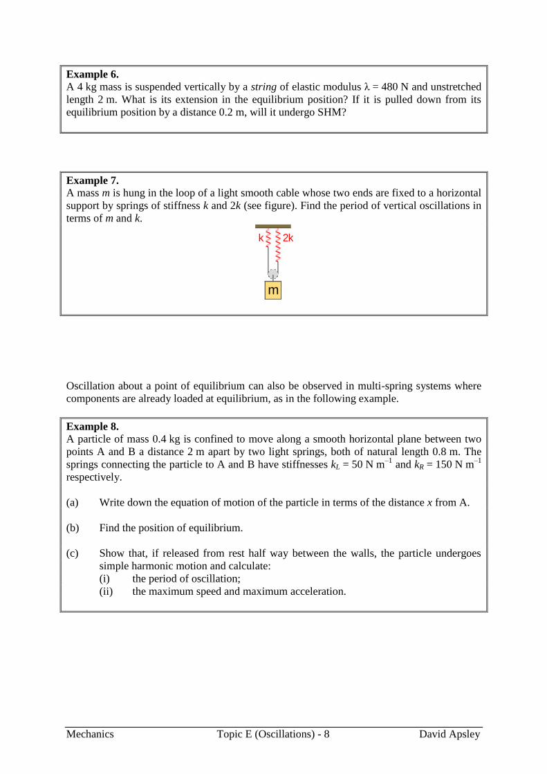
Example 7.
A mass m is hung in the loop of a light smooth cable whose two ends are fixed to a horizontal
support by springs of stiffness k and 2k (see figure). Find the period of vertical oscillations in
terms of m and k.
Oscillation about a point of equilibrium can also be observed in multi-spring systems where
components are already loaded at equilibrium, as in the following example.
Example 8.
A particle of mass 0.4 kg is confined to move along a smooth horizontal plane between two
points A and B a distance 2 m apart by two light springs, both of natural length 0.8 m. The
springs connecting the particle to A and B have stiffnesses kL = 50 N m–1
and kR = 150 N m–1
respectively.
(a) Write down the equation of motion of the particle in terms of the distance x from A.
(b) Find the position of equilibrium.
(c) Show that, if released from rest half way between the walls, the particle undergoes
simple harmonic motion and calculate:
(i) the period of oscillation;
(ii) the maximum speed and maximum acceleration.
m
2kk

Mechanics Topic E (Oscillations) - 9 David Apsley
2.6 Small-Amplitude Approximations
Many oscillatory systems do not undergo exact simple harmonic motion (where the restoring
force is proportional to a displacement), but their motion is approximately SHM provided that
the amplitude of oscillation is small. Such small-amplitude approximations are particularly
common for rotational motion about a fixed point (where the restoring torque is often
provided by gravity or elasticity) and rely on the approximations
)θ1 sometimes,(1θcos
θθsin
2
21
(12)
when θ is measured in radians. These may be derived
formally by power-series expansions, but their essential
validity is easily seen geometrically (see right).
The following table shows that the approximation for sin θ is accurate to about 1% or better
for angles as large as 15˚. If a structural member were actually displaced by this much then
oscillation would be the least of your worries!
θ (degrees) 5 10 15 20
θ (radians) 0.0873 0.175 0.262 0.349
sin θ 0.0872 0.174 0.259 0.342
Important warning: duplication of notation
When considering rotational oscillations we will run into problems with the same symbols
being used for different quantities.
T is used for both torque and period of oscillation (and sometimes tension); in this
section we will use it to mean torque and write “period” out in full.
ω is used for both natural circular frequency and angular velocity; while dealing with
oscillations we shall reserve it to mean the natural circular frequency and write θ or
dθ/dt for the angular velocity.
2.6.1 Rotational Oscillations Driven by Gravity – Compound Pendulum
In a simple pendulum all the mass is concentrated at one point. This can be treated using
either the momentum or angular-momentum equations. In a compound pendulum the mass is
distributed; the system must be analysed by rotational dynamics.
In the absence of friction, two forces act on the body: the weight of the
body (which acts through the centre of gravity) and the reaction at the
axis. Only the former has any moment about the axis.
Let the distance from axis to centre of gravity be L and let the angular
displacement of line AG from the vertical be θ.
The line of action of the weight Mg lies at a distance L sin θ from the
axis of rotation, and hence imparts a torque (moment of force) of
magnitude θsinLMgT and in the opposite sense to θ. The
rotational equation of motion is
L
Mg
A
G
sin
1

Mechanics Topic E (Oscillations) - 10 David Apsley
torque = moment of inertia × angular acceleration
2
2
d
θd
tIT
Hence,
2
2
d
θdθsin
tILMg
For small oscillations, θθsin , so that
θ
d
θd2
2
I
MgL
t
This is SHM with natural circular frequency I
MgLω .
Example 9.
A uniform circular disc of radius 0.5 m is suspended from a horizontal axis passing through a
point halfway between the centre and the circumference. Find the period of small oscillations.
Example 10. (Exam 2017)
A uniform circular disk of mass 3 kg and radius 0.4 m is suspended from a horizontal axis
passing through a point on its circumference and perpendicular to the plane of the disk. A
small particle of mass 2 kg is attached to the other side of the disk at the opposite end of a
diameter.
(a) Find the moment of inertia of the combination about the given axis.
(b) Find the period of small oscillations about the axis.
Axis
3 kg
2 kg

Mechanics Topic E (Oscillations) - 11 David Apsley
Example 11.
A pub sign consists of a square plate of mass 20 kg and sides 0.5 m, suspended from a
horizontal bar by two rods, each of mass 5 kg and length 0.5 m. The sign is rigidly attached to
the rods and swings freely about the bar. Find the period of small oscillations.
2.6.2 Rotational Oscillations Driven By Elastic Forces
If the rotational displacement θ is small then the additional extension of a spring at distance r
from an axis is essentially the length of circular arc:
θrx
This gives a force of magnitude
)θ(rkkxF
opposing the displacement and hence a torque of
magnitude Fr acting in the opposite direction to the
rotational displacement:
θ2krT
Example 12.
A uniform bar of mass M and length L is allowed to pivot about a horizontal axis though its
centre. It is attached to a level plane by two equal springs of stiffness k at its ends as shown.
Find the natural circular frequency for small oscillations.
The Dogand Duck
0.5 m
0.5 m
0.5 m
L
k k
axis r
r

Mechanics Topic E (Oscillations) - 12 David Apsley
2.7 Derivation of the SHM equation from Energy Principles
For a body, of mass m, subject only to elastic forces with stiffness k, the total (i.e. kinetic +
potential) energy is constant:
constantkxmv 2
212
21
Differentiating with respect to time gives
0)(
d
d 2
212
21 kxmv
t
Apply the chain rule to each term:
0
d
d
d
d
t
xkx
t
vmv
Replacing v by dx/dt:
0
d
d
d
d
d
d2
2
t
xkx
t
x
t
xm
Dividing by dx/dt:
0
d
d2
2
kxt
xm
Hence,
0ω
d
d 2
2
2
xt
x (
m
k2ω )
Example 13. A sign of mass M hangs from a fixed support by two rigid rods of negligible mass and length
L (see below). The rods are freely pivoted at the points shown, so that the sign may swing in
a vertical plane without rotating, the rods making an angle θ with the vertical.
(a) Write exact expressions for the potential energy and kinetic energy of the sign in
terms of M, L, g, the displacement angle θ and its time derivative θ .
(b) If the sign is displaced an angle θ = p/3 radians and then released, find an expression
for its maximum speed.
(c) Find an expression for the total (i.e. kinetic + potential) energy using the small-angle
approximations θθsin , 2
21 θ1θcos .
(d) Show that, for small-amplitude oscillations, the assumption of constant total energy
leads to simple harmonic motion, and find its period.
M
LL

Mechanics Topic E (Oscillations) - 13 David Apsley
3. DAMPED FREE OSCILLATION
All real dynamical systems are subject to friction, which opposes relative motion and
consumes mechanical energy. For a system undergoing free oscillation, we shall show that:
moderate damping decaying amplitude and reduced frequency;
large damping oscillation prevented.
The level at which oscillation is just suppressed is called critical damping.
3.1 The Equation of Motion
Friction always acts in a direction so as to oppose relative motion. For a frictional force that
depends on velocity, the damping force is often modelled as
t
xcFd
d
d (13)
c is the viscous damping coefficient. If x is a displacement then c has units of N s m–1
. In
practice, c may vary with velocity, but a useful analysis may be conducted by assuming it is a
constant, in which case the damping is termed linear.
The equation of motion (“F = ma”) for a damped mass-spring system is
2
2
d
d
d
d
t
xm
t
xckx
or
0d
d
d
d2
2
kxt
xc
t
xm (14)
Dividing by m, this can be written
0ωd
d)(
d
d 2
2
2
xt
x
m
c
t
x (15)
where mk/ω is the natural frequency of the undamped system.
The undamped system (c = 0) has solutions of the form )ωsin( tA . In the presence of
damping we expect the solution to decay in magnitude and, possibly, have a slightly different
frequency. Hence we might anticipate solutions of the form
)ωsin(e λ tAx d
t (16)
where A and are arbitrary constants and λ and ωd are to be found. If you don’t like the
analysis which follows, you can try simply substituting this into equation (15) and (after quite
a lot of algebra) deriving the same results as below.
3.2 Solution For Different Damping Levels
Equation (15) is a homogeneous, linear, second-order differential equation with constant
coefficients. Hence, following the method taught in your maths course we seek solutions of
the form:
ptAx e
where p is a constant to be evaluated. Substituting in (15) we obtain the auxiliary equation
m
k
xc

Mechanics Topic E (Oscillations) - 14 David Apsley
0ω22 pm
cp
with roots
1)ω2
(ω2
ω2
ω4)(2
22
m
c
m
cm
c
m
c
p (17)
(For convenience) we define
ω2
ζm
c (damping ratio) (18)
Then
1ζωωζ 2 p (19)
As you know from your maths course, there are 3 possibilities, depending on the sign of the
quantity under the square root (here, 1ζ 2 ) in equation (19):
1. two complex conjugate roots if ζ < 1;
2. two distinct negative real roots if ζ > 1;
3. two equal (negative, real) roots if ζ = 1.
For complex conjugate roots ( ir ppp i )the general solution can be written
)sincos(eeeii
tpDtpCBAx ii
tptptptptp ririr
where A and B (or C and D) are arbitrary constants. The last bracket also has an equivalent
amplitude/phase-angle form.
Case 1: ζ < 1 ( c < 2mω): under-damped system
The general solution may be written
)ωsin(e λ tAx d
t (20)
where
2ζ1ωω d , m
c
2ωζλ (21)
There is oscillation with reduced amplitude (decaying exponentially as tλe ) and reduced
frequency, ωd.
The amplitude reduction factor over one cycle ( π2ω td or dt ω/π2 ) is
}ζ1
πζ2exp{
2 (22)
This may be used to determine the damping ratio ζ experimentally.
Case 1 also includes the special case of no damping (ζ = 0), in which case λ = 0 and ωd = ω.

Mechanics Topic E (Oscillations) - 15 David Apsley
Case 2: ζ > 1 (c > 2mω): over-damped system
The general solution is of the form
ttBAx 21 λλ
ee
(23)
where
)1ζζ(ωλ 2
2,1 (24)
There is no oscillation and, as both of the roots p are negative (i.e. λ positive), the
displacement decays to zero, more slowly as the damping ratio ζ increases.
Case 3: ζ = 1 (c = 2mω): critically-damped system
The general solution has the form:
tBtAx ωe)( (25)
There is no oscillation and the amplitude decays rapidly to zero.
Summary
The damped mass-spring equation
0
d
d
d
d2
2
kxt
xc
t
xm
has solutions that depend on:
undamped natural frequency: m
kω
damping ratio: ω2
ζm
c
● If ζ< 1 the system is under-damped, oscillating, but with exponentially-decaying
amplitude and reduced frequency 2ζ1ωω d .
● If ζ > 1 the system is over-damped and no oscillation occurs.
● The fastest return to equilibrium occurs when the system is critically damped (ζ = 1).

Mechanics Topic E (Oscillations) - 16 David Apsley
Example.
m = 1 kg, k = 64 N m–1
ω = 8 rad s–1
x0 = 0.05 m, 0)/dd( 0 tx .
Cases in the graph:
c = 1.6 N s m–1
(ζ = 0.1)
c = 16 N s m–1
(ζ = 1)
c = 64 N s m–1
(ζ = 4)
Exercise. Use Microsoft
Excel or any other computer
package to compute and plot
the solution for various
combinations of m, k, c.
Example 14.
Analyse the motion of the system shown. What is the damping ratio? Does it oscillate? If so,
what is the period? What value of c would be required for the system to be critically damped?
Example 15. (Exam, May 2016)
A carriage of mass 20 kg is attached to a wall by a spring of stiffness 180 N m–1
. When
required, a hydraulic damper can be attached to provide a resistive force with magnitude
proportional to velocity; the constant of proportionality c = 40 N/(m s–1
).
(a) If the carriage is displaced, write down its equation of motion, in terms of the
displacement x, in the case when the hydraulic damper is in place.
(b) If there is no damping, find the period of oscillation.
(c) If the hydraulic damper is attached, find the period of oscillation and the fraction by
which the amplitude is reduced on each cycle.
Try this question from first principles, rather than citing damping formulae.
40 kg
c = 60 N s/m
k = 700 N/m
20 kg
c = 40 N/(m/s)
k = 180 N/m
x
-0.05
-0.04
-0.03
-0.02
-0.01
0.00
0.01
0.02
0.03
0.04
0.05
0.0 0.5 1.0 1.5 2.0 2.5 3.0
dis
pla
cem
en
t (m
)
time (s)
over-damped
criticallydamped
under-damped

Mechanics Topic E (Oscillations) - 17 David Apsley
4. FORCED OSCILLATION
Systems that oscillate about a position of equilibrium under restoring forces at their own
“preferred” or natural frequency are said to undergo free oscillation.
Systems that are perturbed by some externally-imposed periodic forcing are said to undergo
forced oscillation. Examples which may be encountered in civil engineering are:
concert halls and stadiums;
bridges (e.g. traffic- or wind-induced oscillations);
earthquakes (the lateral oscillations of the foundations are equivalent to periodic
forcing in a reference frame moving with the surface).
The natural frequency and damping ratio are important parameters for systems responding to
externally-imposed forces. Large-amplitude oscillations occur when the imposed frequency is
close to the natural frequency (the phenomenon of resonance). In general, the system’s free-
oscillation properties will affect both the amplitude and the phase of response to external
forcing.
4.1 Mathematical Expression of the Problem
The general form of the equation of motion with harmonic forcing is
tFt
xckx
t
xm Ωsin
d
d
d
d02
2
(26)
or
tm
Fx
t
x
m
c
t
xΩsinω
d
d
d
d 02
2
2
(27)
where the undamped natural frequency is given by
m
k2ω
Second-order differential equations of the form (27) are dealt with in more detail in your
mathematics courses. The general solution is the sum of a complementary function
(containing two arbitrary constants and obtained by setting the RHS of (27) to 0) and a
particular integral (which is any particular solution of the equation and is obtained by a trial
function based on the nature of the RHS). The complementary function is a free-oscillation
solution and, if there is any damping at all, will decay exponentially with time. The large-
time behaviour of the system, therefore, is determined by the particular integral which, from
the form of the RHS, should be a combination of sin Ωt and cos Ωt.
m
k
xc
F sin t0

Mechanics Topic E (Oscillations) - 18 David Apsley
4.2 Static Load
A useful comparison is with the displacement under a steady load of the same amplitude F0,
rather than a variable load tF Ωsin0 . The steady-state displacement xs is given by the position
of static equilibrium:
0Fkxs
whence
2
00
ωm
F
k
Fxs (28)
4.3 Undamped Forced Oscillation
In the special case of no frictional damping, the
equation of motion is
t
m
Fx
t
xΩsinω
d
d 02
2
2
The form of the forcing function suggests a particular integral of the form tCx Ωsin . By
substituting this in the equation of motion to find C, one finds that
2222
0
ω/Ω1)Ωω(
sx
m
FC (29)
where, as above, 2
0 ω/mFxs is the displacement under a static load of the same amplitude.
Hence the magnitude of forced oscillations is Mxs, where the amplitude ratio or
magnification factor M is given by
22 ω/Ω1
1
M (30)
Key Points
(1) The response of the system to external forcing depends on the ratio of the forcing
frequency Ω to the natural frequency ω.
(2) There is resonance (M ) if the forcing frequency approaches the natural
frequency (Ω ω).
(3) If Ω < ω the oscillations are in phase with the forcing (C has the same sign as F0),
because the system can respond fast enough.
(4) If Ω > ω the oscillations are 180 out of phase with the forcing (C has the opposite
sign to F0) because the imposed oscillations are too fast for the system to follow.
(5) If Ω >> ω (very fast oscillations) the system will barely move (C 0).
mk
x
F sin t0
Mechanics Topic E (Oscillations) - 19 David Apsley
4.4 Damped Forced Oscillation
The complete analysis of oscillations for a SDOF system involves forced motion and
damping. The equation of motion is
t
m
Fx
t
x
m
c
t
xΩsinω
d
d)(
d
d 02
2
2
Because of the dx/dt term, a particular integral must contain both tΩsin and tΩcos .
Substituting a trial solution of the form
tDtCx ΩcosΩsin
produces, after a lot of algebra, a solution (optional exercise) of the form
ss xDxC22222222
22
)ω/Ωζ2()ω/Ω1(
ω/Ωζ2,
)ω/Ωζ2()ω/Ω1(
ω/Ω1
(31)
where, as in Section 3, the damping ratio is
ω2ζ
m
c
and the displacement under static load is
2
0 ω/mFxs
This is most conveniently written in the amplitude/phase-angle form
)Ωsin( tMxx s (32)
where the amplitude ratio M is given by
2222
22
)ωΩζ2()ω/Ω1(
1
/x
DCM
s
(33)
and the phase lag by
22 ω/Ω1
ω/Ωζ2tan
C
D (34)
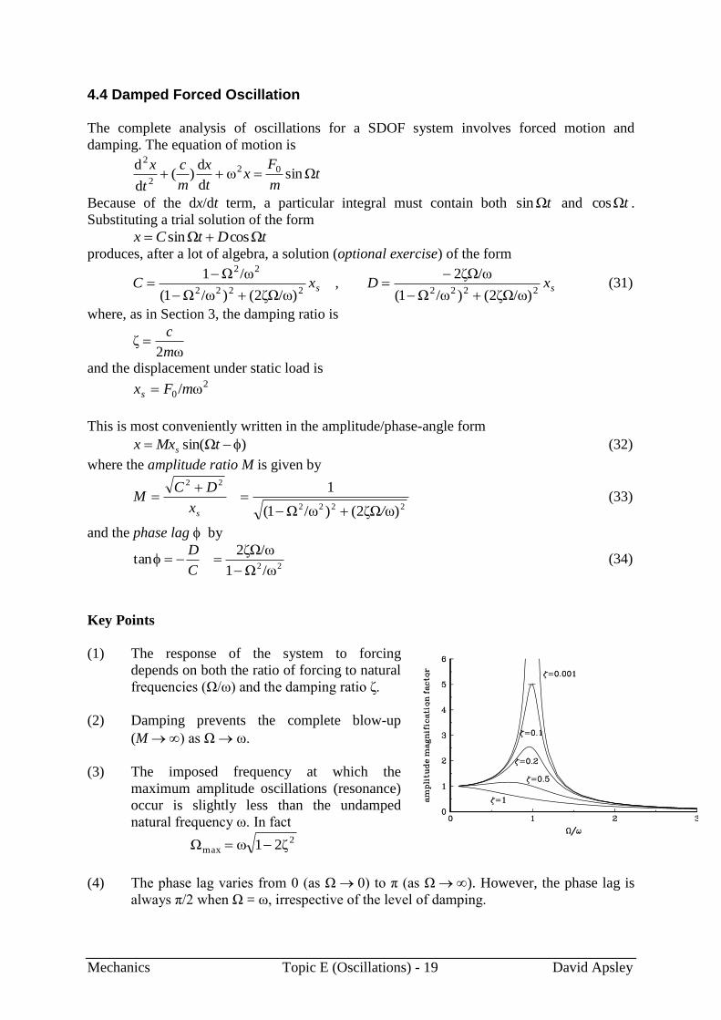
Key Points
(1) The response of the system to forcing
depends on both the ratio of forcing to natural
frequencies (Ω/ω) and the damping ratio ζ.
(2) Damping prevents the complete blow-up
(M ) as Ω ω.
(3) The imposed frequency at which the
maximum amplitude oscillations (resonance)
occur is slightly less than the undamped
natural frequency ω. In fact 2
max ζ21ωΩ
(4) The phase lag varies from 0 (as Ω 0) to π (as Ω ). However, the phase lag is
always π/2 when Ω = ω, irrespective of the level of damping.

Mechanics Topic E (Oscillations) - 20 David Apsley
Example 16.
Write down general solutions for the following differential equations:
(a) 124d
d2
2
xt
x
(b) txt
x
t
x2sin130155
d
d4
d
d2
2
Example 17. (Meriam and Kraige, modified)
The seismometer shown is attached to a structure which has a horizontal harmonic oscillation
at 3 Hz. The instrument has a mass m = 0.5 kg, a spring stiffness k = 150 N m–1
and a viscous
damping coefficient c = 3 N s m–1
. If the maximum recorded value of x in its steady-state
motion is 5 mm, determine the amplitude of the horizontal movement xB of the structure.
x (t)B
mc
x
k

Mechanics Topic E (Oscillations) - 21 David Apsley
Numerical Answers to Examples in the Text
Full worked answers are given in a separate document online.
Example 1.
2.01 s
Example 2.
(a) ω = 3, A = 13, = tan–1
(12/5) = 1.18 radians = 67.4
(b) ω = 2, A = 5, = tan–1
(–4/3) = 2.21 radians = 126.9
Example 3.
(a) k = 160 N m–1
; (b) 4 rad s–1
; (c) 0.637 Hz; (d) 1.57 s; (e) 0.4 m s–1
Example 4.
(b) 0.679 s; 0.3 m; (c) 2.78 m s–1
; 25.7 m s–2
; (d) 2.07 m s–1
Example 5.
(a) k = 400 N m–1
; (b) 0.392 m; (c) 1.26 s
Example 6.
0.164 m; no (the string becomes unstretched).
Example 7.
k
m
2
3π
Example 8.
(a) )1.1(500d
d2
2
xt
x; (b) x = 1.1 m; (c) (i) 0.281 s; (ii) 2.24 m s
–1; 50 m s
–2
Example 9.
1.74 s
Example 10.
(a) 2.0 kg m2; (b) 1.70 s.
Example 11.
1.69 s
Example 12.
M
k6
Example 13.
(a) constantMgL θcosPE , 22
21 θKE ML ; (b) gL ;

Mechanics Topic E (Oscillations) - 22 David Apsley
(c) constantMgLML 2
2122
21 θθ ; (d)
g
Lπ2
Example 14.
It does oscillate; ζ = 0.179, period = 1.53 s; for critical damping, c = 335 N s m–1
Example 15.
(a) 09d
d2
d
d2
2
xt
x
t
x;
(b) 2.09 s
(c) 2.22 s; 0.109
Example 16.
(a) 32sin2cos tDtCx
(b) tttDtCx t 2sin22cos163)sincos(e 2
Example 17.
1.77 mm