TOPIC 2TOPIC 2

The Supply Side of the Economy

2

Goals of Lecture 2

• Introduce the supply side of the macro economy.

• Discuss how countries grow and why some countries grow faster than others.

• Discuss labor productivity o What does it mean? o How does it respond coming out of recessions?

• Determine how wages are set in an economy. Determine why people work.

• Understand where unemployment comes from.

3

The Production Function

• GDP (Y) is produced with capital (K, price-weighted) and labor (N, hours):

Y = A F(K,N)

• Sometimes, I will modify the production function such that:

Y = A F(K,N, other inputs) – where other inputs include energy/oil!

• Realistic Example is a Cobb Douglas function for F(.):

Y = A K.3 N.7

A is Total Factor Productivity (TFP), an index of efficiency (technology)

MUST READ: NOTES 3 (my text posted on the teaching page) on the aggregate production function

4

Measurement

• Y is GDP (measured in dollars). As noted above, we want to measure Y in “real” dollars.<<you should know what this means from Notes 1 of the text>>.

• For our Cobb Douglas production function (previous slide), N and K are both measured in dollars.

– N often is measured in total wage bill

– K often is measured as the replacement cost of capital

• However, in practice, N can be measured in different ways (hours worked, number of workers).

– Wage bill is the preferred method (takes into account “skill” differentials).

– However, we will often talk about standard of livings which is income per capita (Y/N ; where Y is income and N is some population measure).

5

Features of the Aggregate Production Function

Define MPN = Marginal Product of Labor = dY/dN

Define MPK = Marginal Product of Capital = dY/dKMath Note: You should be comfortable taking these simple partial derivatives– if you are

not, practice this for the quizzes and exams.

Diminishing Marginal Products

From Cobb-Douglas: MPN = .7 A (K/N).3 = .7 (Y/N)

Fixing A and K, MPN falls when N increases

MPK = .3 A (N/K).7 = .3 (Y/K)

Fixing A and N, MPK falls when K increases

Complementarity Across Inputs

Increasing A or K, increases MPN

Increasing A or N, increases MPK

6

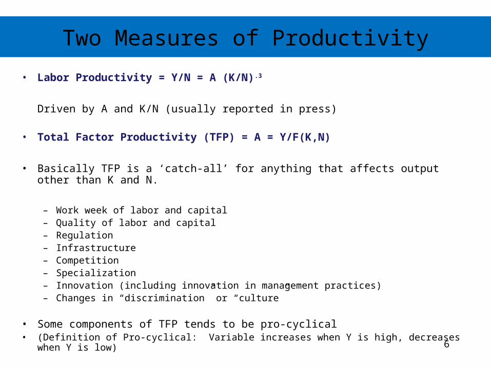
Two Measures of Productivity

• Labor Productivity = Y/N = A (K/N).3

Driven by A and K/N (usually reported in press)

• Total Factor Productivity (TFP) = A = Y/F(K,N)

• Basically TFP is a ‘catch-all’ for anything that affects output other than K and N.

– Work week of labor and capital – Quality of labor and capital– Regulation– Infrastructure– Competition– Specialization– Innovation (including innovation in management practices)– Changes in “discrimination” or “culture”

• Some components of TFP tends to be pro-cyclical • (Definition of Pro-cyclical: Variable increases when Y is high, decreases when Y is low)

Sub-Section ASub-Section A

Economic Growth

8

Growth Accounting

Y = A K.3 N .7 (our production function)

%ΔY = %ΔA + .3%ΔK + .7%ΔN

Output, in a country grows from:

Growth in TFP (see entrepreneurial ability, education, roads, technology, etc.)

Growth in Capital (machines, equipment, plants)

Growth in Hours (workforce, population, labor participation, etc).

Perhaps, we care about growth in Y/pop or Y/N (per capita output).

%Δ(Y/pop) = %ΔA + .3%Δ(K/pop) + .7%Δ(N/pop)

or

%Δ(Y/N) = %ΔA + .3%Δ(K/N)

9

Productivity During Recession

Y/N evolves by:

Y falling (holding N constant) decreases Y/N

N falling (holding Y constant) increases Y/N

In recessions, both Y and N fall.

The question of interest:

Does Y or N fall more during a recession?

10

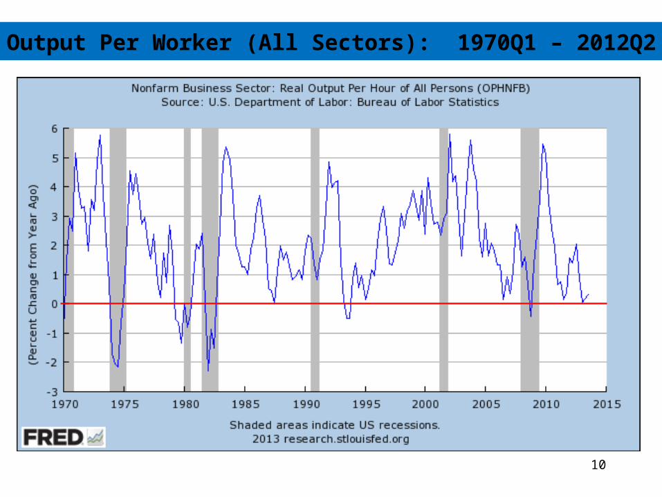
Output Per Worker (All Sectors): 1970Q1 – 2012Q2

11

Summary

During recent recessions:

N falls more than Y

Y/N (a measure of productivity) actually increases

We are producing more stuff – with less workers – during the recession!

Note: The fact that productivity increases during recent recoveries is directly linked to the fact that recent recoveries have been “jobless” (discussed in lecture 1). The economy recovers but employment lags.

Why are there jobless recoveries?

12

The Role of Investment and Growth

Does a one time increase in investment today increase Y/N today? YES!

Does a one time increase in investment today cause a sustained increase in Y/N into the future? No!

Back of our mind equations:

S = I + NX (From the first lecture). Notice the link between saving and investment.

K(t+1) = (1-δ) K(t) + I(t) Definition of Capital Stock Evolution

orΔK(t, t+1) = I(t) - δ K(t)

All else equal (i.e. holding N constant), increasing I causes K tomorrow to increase causing K/N tomorrow to increase (i.e. Y/N tomorrow increases).

13

Time Path of Capital Stock: One Time Increase in I

time

K

No investment

t+1

No investment

Suppose there is a one time increase in investment at time t (perhaps due to an investment tax credit). Suppose no investment either prior to or after the tax credit.

14

Can Higher Investment Lead to Infinite Growth?

Does a sustained increase in investment increase Y/N today? YES!Does a sustained increase in investment cause a sustained increase in Y/N?

No!

Suppose I is fixed at a high level and that K initially is sufficiently small.

K grows if I > δ K: But, notice that δK is also growing each period. (Summary: To start, higher I will lead to higher K and Y/N will increase).

Eventually, however, I will converge towards δK More and more of the investment is going to replace outdated capital and the capital stock will grow by smaller and smaller rates. The increase in Y/N will converge back to zero.

Summary: High levels of investment will increase the capital stock and output, but both K and Y will eventually converge to a fixed level.

15

Time Path of K: Permanent Increase in I

time

K

No investment

t+1

Suppose there is a permanent increase in investment at time t. Suppose no investment prior to t. In all periods after t, the level of investment remains fixed at the level in t.

The new level of investment has successively less effectdue to growing depreciation of the capital stock.

16

Can Higher Investment Growth Cause Infinite Growth?

If a one time increase in I gives an increase in Y, why not continuously raise I to higher and higher amounts??? Answer: Diminishing MPK!!!

MPK = .3 A (N/K) .7; As K increases, MPK falls. As K goes to infinity, MPK goes to zero (Y stops increasing).

Suppose, we keep rising I (each year), K will increase by the amount of I (after controlling for depreciation), but Y will increase by continuously smaller and smaller amounts.

Remember Y = C + I + G + NX. I/Y (investment rate) is bounded by 1 (if you invest all your output). This caps the increase in I. I cannot grow forever!

Continuously increasing I will NOT lead to sustained economic growth.

NOTE: Investment decisions are NOT made in the dark (i.e. something must drive firm investment!)

17

What Causes Sustained Growth ?

Sustained Increases in the growth of A are the only thing that can cause a sustained growth in Y/N.

Empirically, when a country exhibits faster Y/N growth …..

33% typically comes from growth in K/N

67% typically comes from growth in A

(where N = employment (not hours) - limited data).

18

Growth Across Countries

Most developed economies grow at the same rate that the “technological frontier” grows.

Some helpful definitions:

Convergence – countries inside of the technological frontier move towards the technological frontier.

Divergence – countries inside of the technological frontier grow at a rate less than the technological frontier.

19

Distribution of World GDP in 2011 (WorldBank, $)

20

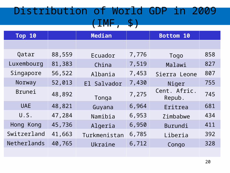
Distribution of World GDP in 2009 (IMF, $)

Top 10 Median Bottom 10

Qatar 88,559  Ecuador 7,776  Togo 858

Luxembourg 81,383  China 7,519  Malawi 827

Singapore 56,522  Albania 7,453  Sierra Leone 807

Norway 52,013  El Salvador 7,430  Niger 755

Brunei 48,892  Tonga 7,275  Cent. Afric. Repub. 745

UAE 48,821  Guyana 6,964  Eritrea 681

U.S. 47,284  Namibia 6,953  Zimbabwe 434

Hong Kong 45,736  Algeria 6,950  Burundi 411

Switzerland 41,663  Turkmenistan 6,785  Liberia 392

Netherlands 40,765  Ukraine 6,712  Congo 328

21

Some Data: Distribution of World GDP in 2000

From Barro, 2003 – includes 147 countries. Horizontal axis is a log scale.All data are in 1995 U.S. dollars.

22

Some Data: Distribution of World GDP in 1960

From Barro, 2003 – includes 113 countries. Horizontal axis is a log scale.All data are in 1995 U.S. dollars.

23

Growth Rate of GDP Per Capita: 1960 - 2000

From Barro, 2003 – includes 111 countries.

24

Relative Growth Rate of GDP Per Capita: 1960 - 1988

U.S. is anchored at 1 in both years. Countries above the line have made gains relative to U.S.

25

Convergence of Income Across U.S. States: 1940 - 1980

AL

AZ

AR

CA

CO

CT

DE

FL

GA

ID

IL

INIA

KSKY

LA

ME

MDMA

MI

MN

MS

MO

MT

NE

NV

NH

NJ

NM

NY

NC

ND

OH

OK

OR

PA

RI

SC

SD

TN

TX

UT

VT

VA

WA

WV WI

WY

.2.4

.6.8

1

Gro

wth

in

Pe

r C

apita I

ncom

e 1

940

-1960

2000 4000 6000 8000 10000 12000Per Capita Income 1940

Fitted values gr_ipc_40_60

Unadjusted 1940-1960Historical Trends in Convergence

26

Convergence of Income Across U.S. States: 1980 - 2000

AL

AZ

AR

CA

CO

CT

DEFL

GA

ID

ILIN

IA KS

KY

LA

MEMD

MA

MI

MN

MSMO

MT

NE

NV

NH

NJ

NM

NY

NC

ND

OH

OK

OR

PARI

SC SDTN

TXUT

VT

VA

WA

WV

WI

WY

.1.2

.3.4

.5G

row

th in

Pe

r C

apita I

ncom

e 1

980

-2000

15000 20000 25000Per Capita Income 1980

Fitted values gr_ipc_80_00

Unadjusted 1980-2000Recent Trends in Convergence

Bonus SectionBonus Section

New Research Project:“The Allocation of Talent and Economic Growth”

(Trying to Shed Light on the Black Box of TFP Growth)

28

Measuring TFP (A)

The way TFP (A) is usually measured is via a statistical decomposition (referred to as the “Solow Residual”).

Remember our assumed production function: Y = AK.3N.7

•Math Note: We are going to transform the production function to make it a little easier to work with (you should get comfortable with this) by taking the logs:

ln(Y) = ln(A) + α0ln(K) + α1ln(N) (where α0 = 1 – α1 ≈ 0.3) (1)

•Given that we measure Y, K and N in the data, we can estimate (1) using standard regression techniques.

•ln(A) is the constant from the regression. This is our standard TFP measure.

29

Measuring TFP

Because A (TFP) is a catch-all term for anything that affects production, the assumed production function does not impose any structure on how to measure the components of TFP.

Economists are very good at measuring the extent to which TFP changes over time within a country.

It is much harder to measure “why” TFP has changed over time.

Economists try to measure this by using detailed firm-level and household-level data to measure production and wages.

30

Our Project

Question 1:

How much of the observed TFP growth in the U.S. since 1960 is due to better labor market outcomes (including human capital formation) for blacks and women?

o A better allocation of resources leads to higher economic growth!

o There have been HUGE changes in the allocation of women and blacks in the labor market since 1960.

Question 2:

How much of the convergence of the U.S. south to the U.S. north is due to a decline in discrimination of the south?

Occupational Sorting Over Time: An Overview

• Fraction of group (white men, white women, black men, black women) aged 25-55 working in the following occupations:

Executives, Mgmt, Architects, Engineers, Math/Computer Science, Natural Scientists, Doctors, and Lawyers.

1960 2006-2008

White Men 21.2% 23.5%

White Women 3.0 (7.3) 17.4 (21.0)

Black Men 2.8 14.6

Black Women 1.0 (2.1) 13.0 (15.2)

Data: U.S. Census and American Community Survey

Occupational Sorting Over Time: An Overview

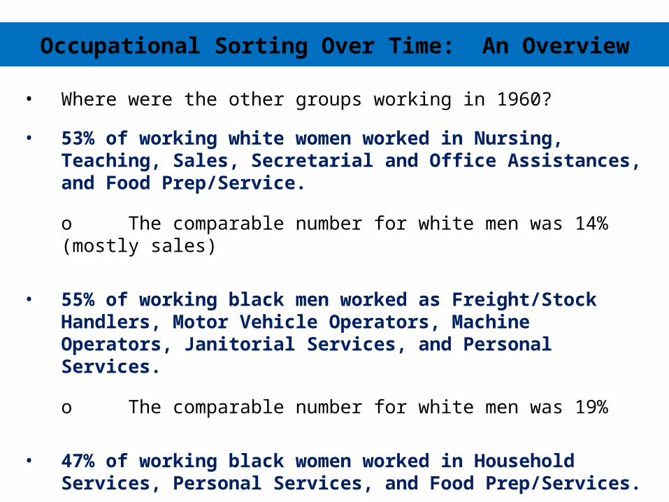
• Where were the other groups working in 1960?

• 53% of working white women worked in Nursing, Teaching, Sales, Secretarial and Office Assistances, and Food Prep/Service.

o The comparable number for white men was 14% (mostly sales)

• 55% of working black men worked as Freight/Stock Handlers, Motor Vehicle Operators, Machine Operators, Janitorial Services, and Personal Services.

o The comparable number for white men was 19%

• 47% of working black women worked in Household Services, Personal Services, and Food Prep/Services.

o The comparable number for white men was 2%

Wage Gaps Over Time: An Overview

• Log difference in annual earnings of full time workers, conditional on experience, hours and occupation controls (relative to White Men)

1960 1980 2008

White Women -0.56 -0.47 -0.26

Black Men -0.37 -0.21 -0.16

Black Women -0.82 -0.47 -0.31

Findings

Macro Implications:

o 15% − 20% of total wage growth in the U.S. between 1960 and 2008 was due to declining frictions for white women, black women, and black men. (Shines some light into the black box of TFP growth)

o Other interesting results:

- Wage growth in the 1970s and the 2000s would have been negative

absent the labor market improvements for blacks and women.

- About 40% of the convergence of the south to the northeast between 1960 and 1980 is due to declining labor market frictions.

- Not much remaining room for growth from this mechanism.

Sub-Section BSub-Section B

The Labor Market

36

Labor Market: Firm Profit Decisions

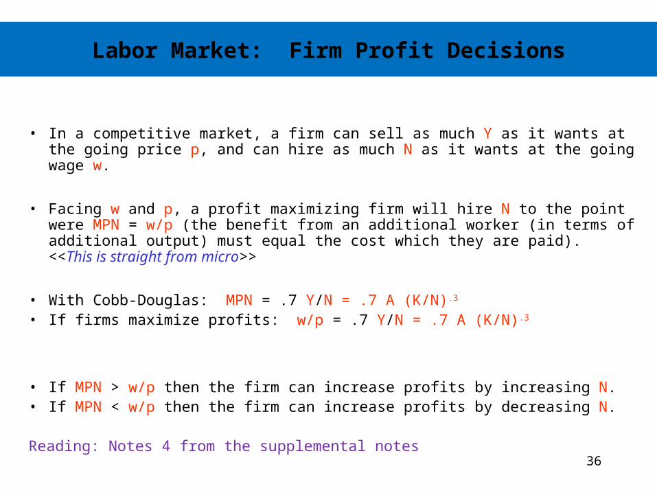
• In a competitive market, a firm can sell as much Y as it wants at the going price p, and can hire as much N as it wants at the going wage w.

• Facing w and p, a profit maximizing firm will hire N to the point were MPN = w/p (the benefit from an additional worker (in terms of additional output) must equal the cost which they are paid). <<This is straight from micro>>

• With Cobb-Douglas: MPN = .7 Y/N = .7 A (K/N).3

• If firms maximize profits: w/p = .7 Y/N = .7 A (K/N).3

• If MPN > w/p then the firm can increase profits by increasing N. • If MPN < w/p then the firm can increase profits by decreasing N.

Reading: Notes 4 from the supplemental notes

37

The Labor Demand Curve

w/p * real wage

MPN = Nd

NN*

38

Notes on the Labor Demand Curve

• Nd slopes downward (Nd = MPN = .7 A * (K/N).3)

• Nd rises with A and K (assumed complementarity across inputs)

• Assumption: Y is not Fixed! Firms optimally choose N, K, Y and (to some extent) A to maximize profits.

• Caveat: Who says that there is a demand for more Y?

– Need to look at the demand side of economy (introduced last -discussed in depth throughout the course).

39

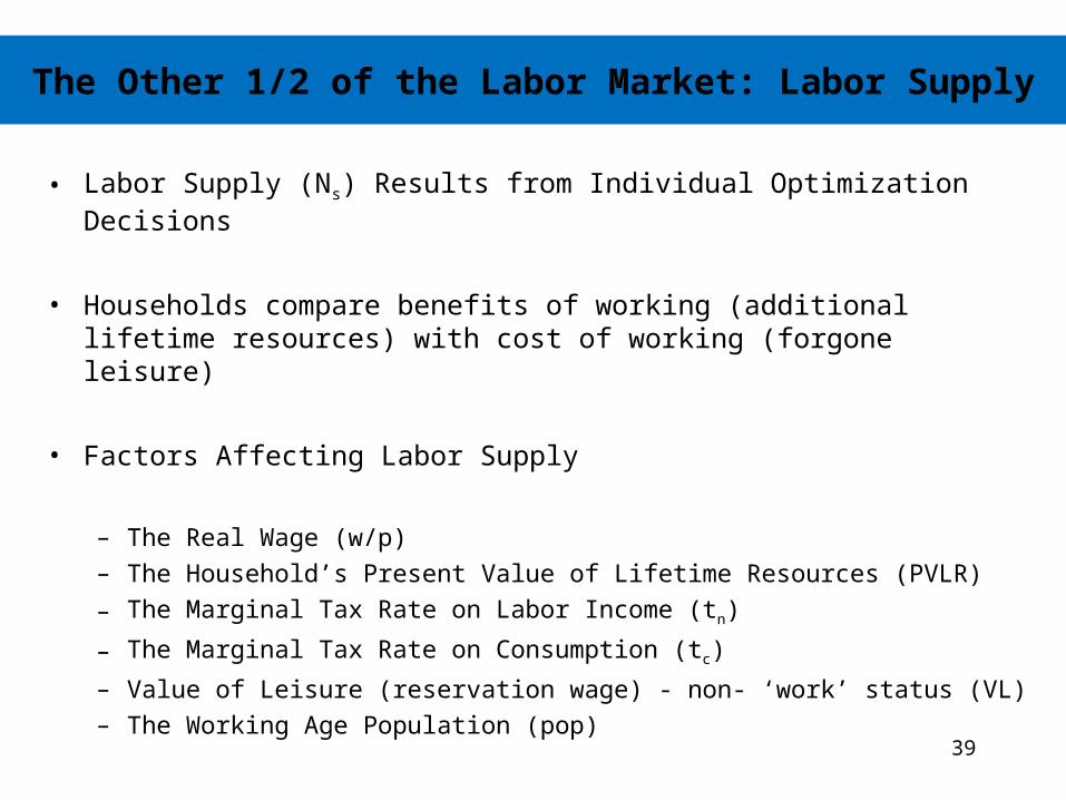
The Other 1/2 of the Labor Market: Labor Supply

• Labor Supply (Ns) Results from Individual Optimization Decisions

• Households compare benefits of working (additional lifetime resources) with cost of working (forgone leisure)

• Factors Affecting Labor Supply

– The Real Wage (w/p)

– The Household’s Present Value of Lifetime Resources (PVLR)

– The Marginal Tax Rate on Labor Income (tn)

– The Marginal Tax Rate on Consumption (tc)

– Value of Leisure (reservation wage) - non- ‘work’ status (VL)

– The Working Age Population (pop)

40

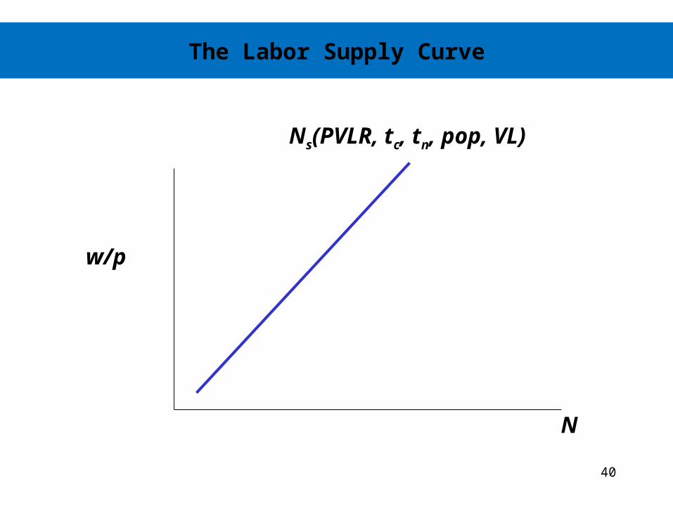
The Labor Supply Curve

w/p

N

Ns(PVLR, tc, tn, pop, VL)

41

Labor Supply Notes (Most Derived From Scratch in Lecture)

• In terms of ‘wages and earnings’, there is both an income and substitution effect - we will look at them separately – BUT in the real world, they often occur jointly!!!!

• The Real Wage - HOLDING PVLR fixed: A higher w/p encourages individuals to substitute away from leisure and toward work (leisure becomes more expensive). This is a substitution effect. <<This is why the labor supply curve slopes upwards!!>>

– Estimating this substitution effect is difficult since PVLR is not easily held constant. Estimates range from 0 - 2% (For a 1% increase in after-tax w/p holding PVLR fixed, labor supply either increases by 0% or 2%). Very Wide Range – little consensus.

• PVLR = initial wealth + present discounted value of earnings

– A higher PVLR induces individuals to work less (lower Ns) for a given after-tax wage, allowing them to enjoy more leisure (If leisure is preferred to work – as I get richer, I can afford to work less).

– PVLR is net of taxes and non-work governmental transfers and inclusive of all other transfers.

42

Labor Supply Notes

• Marginal tax rate on labor income - Should have same substitution effect as the before tax real wage. Studies of the 1986 U.S. Tax Reform found that only high-earning married women worked more in response to lower marginal income tax rates.

• Marginal tax rate on consumption - see above

• Value of Leisure - If leisure/no-work becomes more/less attractive, households will less/more (reservation wage). (Welfare programs, child care, etc.).

• Working Age Population: Usually defined as 16-64. (Includes changes in Labor Force Participation Rates)

Reading: #29

43

Recap on Labor Supply

• Substitution Effect:

– For a given PVLR, a higher after tax wage increases NS.

(This is why Labor Supply Curve Slopes Upward)

• Income Effect

– For a given after-tax wage, higher PVLR decreases Ns.

• Evidence:

– Weak Consensus is that, with equal (%) increase in PVLR and the after-tax wage, Ns falls (income effect dominates).

44

Temporary Increase in A

w/p

N

Ns(PVLR, tc, tn, pop, VL)

N d(A,K)

N*

w/p *

45

Permanent Increase in A

w/p

N

Ns(PVLR, tc, tn, pop, VL)

N d(A,K)

N*

w/p *

46

Can Technological Progress Destroy jobs?

Facts: A, N, w/p are trending up over time.

N/pop is trending down (except in U.S. since 1980).

Higher A countries have higher w/p and lower N/pop.

Implications:

Adjusting for pop, higher A goes with lower N.

Higher A reduces Nd and destroys jobs? - NO!

Labor Demand Increases.

Higher A increases PVLR and reduces Ns - The Effect on Labor Supply is to fall.

47

Permanent Increase in Population

w/p

N

Ns(PVLR, tc, tn, pop, VL)

N d(A,K)

N*

w/p *

48

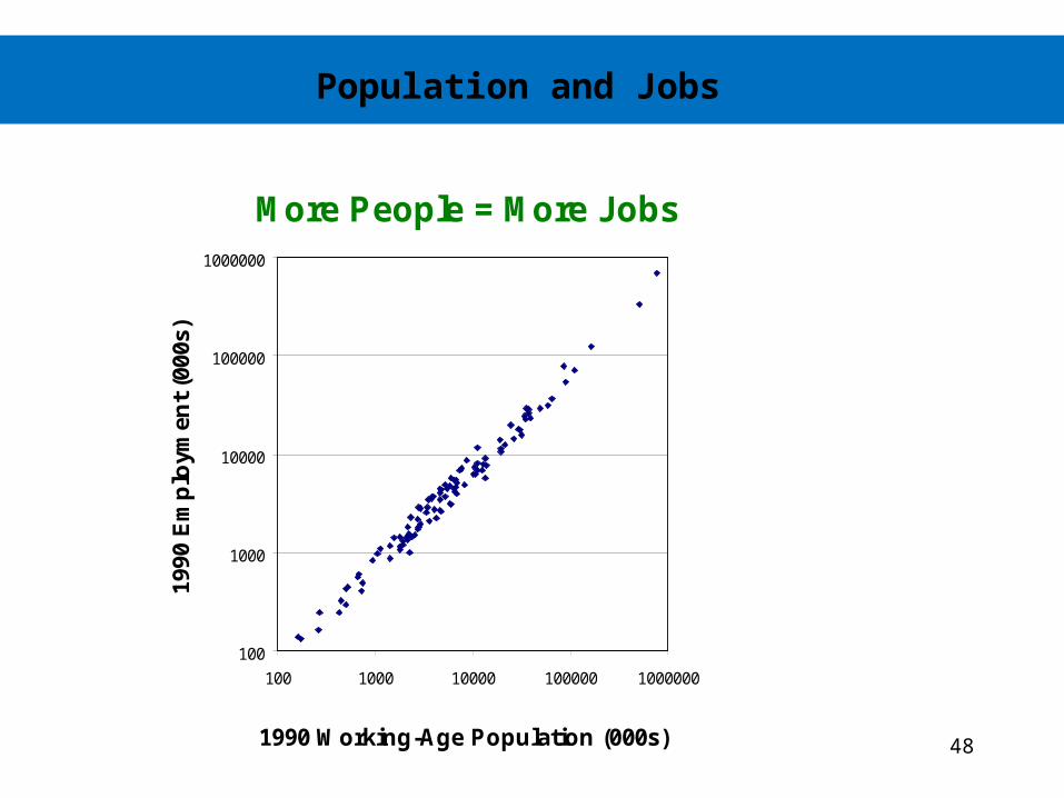
Population and Jobs

More People = More Jobs

100

1000

10000

100000

1000000

100 1000 10000 100000 1000000

1990 Working-Age Population (000s)

1990

Em

plo

ymen

t (0

00s)

49

Temporary Increase in Taxes (tc or tn)

w/p

N

Ns(PVLR, tc, tn, pop, VL)

N d(A,K)

N*

w/p *

50

Permanent Increase in Taxes (tc or tn)

w/p

N

Ns(PVLR, tc, tn, pop, VL)

N d(A,K)

N*

w/p *

51

Labor Market Equilibrium (in long run!)

• We define Long Run Equilibrium in macroeconomics as occurring when the labor market clears.

• By definition, long run macro equilibrium exists when N = N*.

• At N*, labor demand = labor supply. So, by definition, all workers who want a job (the suppliers) are able to find a firm looking for a worker (the demanders).

• Implies that cyclical unemployment = zero at N*.• Long run equilibrium is characterized by zero cyclical unemployment!

• It is an equilibrium in that there is no incentive for real wages to change at N*

• Real wages (w/p) has two components: nominal wages (w) and the price level (p).

• Note: Y* (by definition) = A K.3(N*).7

• Y* is the long run equilibrium level of output (output where labor market is in equilibrium)

52

Our First Aggregate Supply Curve….

• Suppose prices (p) increase. What happens in the labor market?

• In terms of equilibrium, nothing happens!• Increasing prices have no effect on labor demand (A and K do not change).• Increasing prices have no effect on labor supply (taxes, population, etc. do

not change).

• You may ask “Doesn’t PVLR change when prices increase???” No!

• As long as nominal wages adjust, real wages will be unchanged when p increases.

• The % change in prices will be match exactly by the % change in nominal wages – real wages will not change (so PVLR will not change).

• No effect on labor supply.

• Key: Because real wages will not change, changes in prices will have NO effect on the labor market (i.e., it will have no effect on N*).

• Conclusion: Changing prices will have NO effect on Y* (since N* is constant).

53

Our First Aggregate Supply Curve……

Y

p

LRAS – Long Run Aggregate Supply Curve

Y*

• If labor market clears, changes in prices will lead to equal changes in nominal wages.As a result, there will be no change in N* and hence, no change in Y*.

• Leads to a vertical LRAS curve. Prices do not affect production in the long run!

54

What Shifts Y*? (the LRAS)

• Anything that affects the labor market will affect Y*!

• If N* increases, Y* will shift to the right.

• If N* decreases, Y* will shift to the left.

• Summary: Y* will shift right if:

– A increases– K increases– population increases– labor income taxes fall (and income effect is small relative to substitution effect)– labor income taxes rise (and income effect is large relative to substitution effect)

Note: The long run aggregate supply curve (LRAS) is NOT the labor supply curve. We have lots of different markets in this class. There will be lots of different supply and demand curves. You need to keep track of them!

55

Things to Remember!

• The demand side of the economy is NOT important for determining Y*!

– All we need to know is A, K and N and we know Y*!

– The demand side of the economy is not important for economic growth!

– Key: If I ever ask you about what determines Y* (i.e., output/income/expenditure in the long run), you should think about A, K and the labor market.

• As a rule, K will be fixed unless I tell you otherwise (for simplicity, you will see why soon).

• Why do we care about the demand side of the economy?

– In the long run, prices will be determined by demand.– Also, LRAS is dependent on labor market being in equilibrium. In the short run, labor

market need not be in equilibrium.– Demand will determine output in the SHORT RUN!

56

Summary….

• In the long run – when labor markets clear.

– Supply side of economy (labor market, K, A, other inputs like oil) determines output.

– Demand side of economy (C+I+G+NX) will determine prices.

• In the short run – when labor markets do not clear:

– Demand and Supply jointly determine prices and output (think of the simple examples I gave graphically in the lecture for topic 1).

– Three outstanding issues (we will get to them soon):

• When is the labor market NOT in equilibrium?• What does the supply curve look like when labor market doesn’t clear?• What determines demand?

57

When are Labor Markets in Disequilibrium?

• Labor market is in disequilibrium when labor demand is not equal to labor supply.

• Any time labor demand = labor supply, there is no cyclical unemployment (by definition)!

• Nominal wages do not adjust to clear the labor market

– We refer to this as ‘sticky’ wages.

– Because of wage contracts (and uncertainty), nominal wages do not always adjust immediately.

– Need a model for short-run disequilibrium --- we will do that in Topic 6.

58

Cyclical Unemployment in Labor Markets

• When do we get cyclical unemployment in our models?

• Cyclical unemployment occurs when there are no jobs available (labor demand) for those with the skills and the desire to work (labor supply) at current wages.

• Cyclical unemployment occurs only in disequilibrium! (when desired labor demand < desired labor supply - at given wages)

w’/p’

Nd

Ns

N(0)N(1)

ab

Unemployment

59

What Have We Learned So Far?

• There are microeconomic fundamentals to the supply side of the economy –

– Capital accumulation, Labor and TFP are important for production AND Growth!!!

• Some countries grow faster than others because they have rapid growth in TFP or K/N.

• Only growth in TFP can lead to sustained growth in Y/N

• How Labor Markets Work - The Role of Taxes, Technological Progress, Capital Accumulation, And Demographics on Wages and Employment.

• Demand is not important for determining long run output (i.e., income, standard of livings, etc.). Supply (production) is the only thing that determines output in the long run!

Exploiting Within-U.S. Variation To Learn About Business Cycle Effects of Labor Markets

My Recent Research on Housing/Manufacturing

Two new papers with Kerwin Charles (Harris School) and Matt Notowidigdo (Booth).

Exploit regional patterns in:

o Manufacturing declines during 2000s (predicted by initial share of manufacturing in metropolitan area in year 2000).

o Housing booms during 2000s (predicted by discrete changes in housing prices in metropolitan area during early 2000s).

Analyze effects of changes on overall employment rates, wages, employment by sector, migration, human capital attainment, etc.

Intuition of the Model: Labor Supply and Labor Demand

Wages

N

Labor Supply

Labor Demand

(W/P)1

N1

(W/P)2

N2

Predicted Manufacturing Change vs. Change in Non-Employment, Non College Men 2000-2007

Bigger Manufacturing Decline

Predicted Manufacturing Change vs. Change in Non-Employment, Non College Men 2000-2007

Bigger Manufacturing Decline

Increase in Non-Employment

Predicted Housing Demand Change vs. Change in Non-Employment, Non College Men 2000-2007

Bigger Housing Demand Shock

Counterfactuals From Our Paper

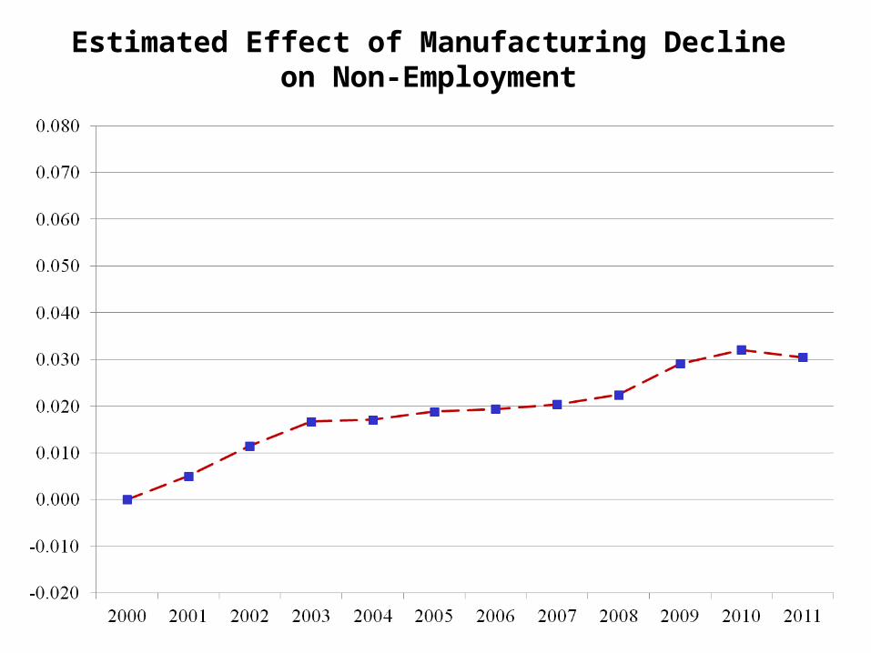
Estimated Effect of Manufacturing Decline on Non-Employment

Estimated Effect of Manufacturing Decline on Non-Employment

~42% Explained

Estimated Effect of Housing Cycle on Non-Employment

Housing Cycle (Construction and Other)

Manufacturing Decline

The Housing Boom Masked The Manufacturing Decline in 2000s

Manufacturing

Data

Housing + Manufacturing

The Housing Boom Masked The Manufacturing Decline in 2000s

Manufacturing

Data

Housing + Manufacturing

34% DuringRecession