Topic 2 Linear Functions - University of Adelaide · Topic 2 Linear Functions –1 0 x 1 –1 y y <...

MathsStart (NOTE Feb 2013: This is the old version of MathsStart. New books will be created during 2013 and 2014)

MATHS LEARNING CENTRE

Level 3, Hub Central, North Terrace Campus

The University of Adelaide, SA, 5005

TEL 8313 5862 | FAX 8313 7034 | EMAIL [email protected]

www.adelaide.edu.au/mathslearning/

Topic 2

Linear Functions

1 –1 0

1

–1

y

x

y < 2x – 1

This Topic...

This module introduces linear functions, their graphs and characteristics. Linear functions

are widely used in mathematics and statistics. They arise naturally in many practical and

theoretical situations, and they are also used to simplify and interpret relationships between

variables in the real world. Other topics include simultaneous linear equations and linear

inequalities.

Author of Topic 2: Paul Andrew

__ Prerequisites ______________________________________________

You will need to solve linear equations in this module. This is covered in appendix 1.

__ Contents __________________________________________________

Chapter 1 Linear Functions and Straight Lines.

Chapter 2 Simultaneous Linear Equations.

Chapter 3 Linear Inequalities.

Appendices

A. Linear Equations

B. Assignment

C. Answers

Printed: 18/02/2013

1 Linear Functions and Straight Lines

1

Linear functions are functions whose graphs are straight lines. The important characteristics of

linear functions are found from their graphs.

1.1 Examples of linear functions and their graphs

Cost functions are commonly used in financial analysis and are examples of linear functions.

Example

The table below shows the cost of using a plumber for between 0 and 4 hours. This plumber has a

$35 callout fee and charges $25 per hour.

Hours 0 1 2 3 4

Cost 35

35 251

35 252

35 25 3

35 25 4

It can be seen from this table that the cost function for the plumber is C = 35 + 25T, where T is the

number of hours worked. This is a linear function and it has a straight line graph.

The graph cuts the C-axis at the point (0, 35), corresponding to the cost of the call out fee when T =

0. The cost then increases steadily at a rate of $25 per hour.

Time (hours)

1 2 3 4 5

150

100

50

0

Cost

($)

C = 35 + 25T

T

C

•

•

•

•

•

Simultaneous Linear Equations 2

Lines of best fit are often used to model the relationship between two variables. A line of best fit is

a straight line that best fits a set of data, and is usually drawn with the aid of a software package like

Excel.

Example

The graph below shows the amount of diesel fuel used by a farmer when ploughing a variety of

paddocks at a constant speed (the data points are indicated by dots). The relationship between fuel

used and time taken is roughly linear (i.e. given by a straight line). The line can be used to estimate

future fuel needs and costs.

When studying the mathematical properties of general linear functions we use x to represent the

independent variable and y to represent the dependent variable. We also place no restrictions on the

domain of the independent variable x. The x- and y-intercepts of linear functions (ie. where the

straight lines cut the x- and y-axes) are important features of linear functions, and are usually shown

on their graphs unless there is a good reason not to.

Example

The graph of the linear function

y 200x100 is shown below. The x-intercept is (0.5, 0) and the

y-intercept is (0, –100). When the value of x increases by 1 unit, the value of y increases by 200

units.

• •

•

•

• •

•

•

•

•

• •

•

•

• •

Die

sel

Fuel

Ploughing Time

Die

sel

Fuel

T

F

3 Linear Functions

Example (See Appendix: Linear Equations)

The x- and y- intercepts of the linear function y = 200x – 100 can be found algebraically as follows:

(a) To find x-intercept:

Put y = 0

200x – 100 = 0

200x = 100

x = 100/200 = 0.5

The x-intercept is (0.5, 0).

(b)

To find y-intercept:

Put x = 0

y = 0 – 100 = –100

The y-intercept is (0, –100).

The quickest way of drawing a straight line graph is to

• find two points on the line, then

• draw a straight line through these two points.

Problems 1.1

Each function below is a linear function, with a straight line graph. Draw each graph, showing the

x- and y-intercepts.

(a)

y 2x1 (b)

y 20x10 (c)

y 0.1(2x1)

(d)

y x (e)

y 2x (f)

y 3x

(g)

f (x)x1 (h)

f (x)2x1 (i)

g(x) 23x

1 –1 0

100

–100

y 200x100

y

x

The x- and y-intercepts are

usually chosen to be the two

points.


1.2 The gradient of a straight line

The gradient (or slope) of a straight line measures its steepness. It is represented by the letter m.

m = gradient = rise

run

When calculating a gradient, a "rise" may be positive, e.g.

or it may be negative, e.g.

The steeper the line, the larger the gradient (in both the positive or negative directions):

10

metres

2

metres

m 2

10 0.2

10

metres

–2

m 2

100.2

m =

0

m = 0.5

m = 1

m = 1.5

m = 2

m = 3 m = 0

m = –0.5

m = –1

m = –1.5

m = –2

m = –3 Notice that angles are

not doubled when

gradients are doubled

5 Linear Functions

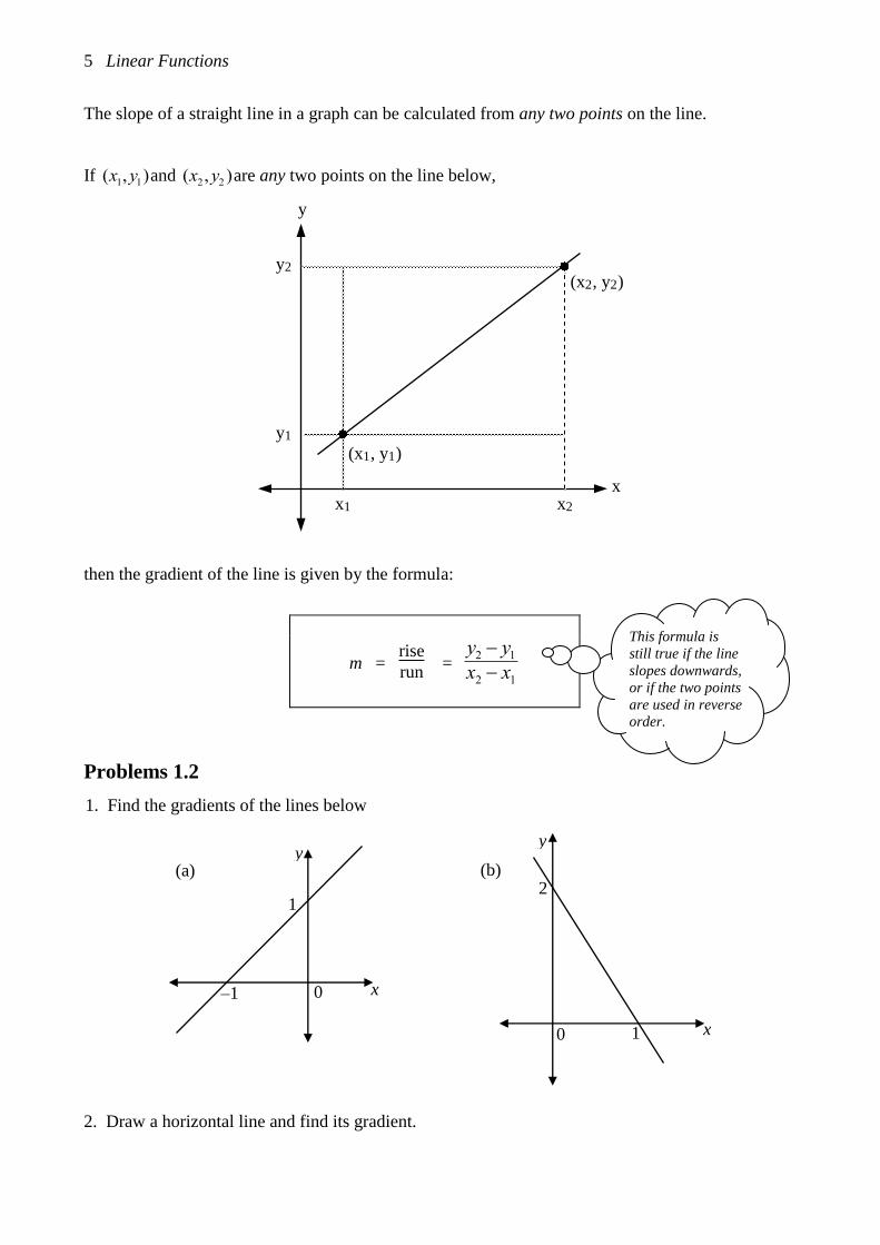
The slope of a straight line in a graph can be calculated from any two points on the line.

If

(x1,y1)and

(x2,y2 )are any two points on the line below,

(x1, y1)

(x2, y2)

x1 x2

y1

y2

y

x

then the gradient of the line is given by the formula:

m = rise

run =

y2 y1x2 x1

Problems 1.2

1. Find the gradients of the lines below

2. Draw a horizontal line and find its gradient.

1

–1 0 x

y (a)

y

x 0 1

2 (b)

This formula is

still true if the line

slopes downwards,

or if the two points

are used in reverse

order.


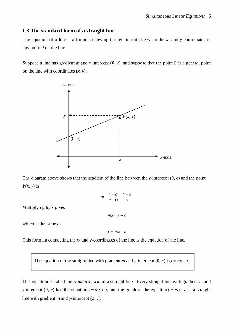
1.3 The standard form of a straight line

The equation of a line is a formula showing the relationship between the x- and y-coordinates of

any point P on the line.

Suppose a line has gradient m and y-intercept (0, c), and suppose that the point P is a general point

on the line with coordinates (x, y).

The diagram above shows that the gradient of the line between the y-intercept (0, c) and the point

P(x, y) is

m y c

x0y c

x.

Multiplying by x gives

mx yc

which is the same as

ymxc

This formula connecting the x- and y-coordinates of the line is the equation of the line.

The equation of the straight line with gradient m and y-intercept (0, c) is

ymxc.

This equation is called the standard form of a straight line. Every straight line with gradient m and

y-intercept (0, c) has the equation

ymxc, and the graph of the equation

ymxc is a straight

line with gradient m and y-intercept (0, c).

y-axis

x-axis

y

x

(0, c)

P(x, y) •

7 Linear Functions

Linear functions are functions that have straight line graphs, so:

A linear function of x has the standard form

f (x)mxc .

Example

The graph of

y 2x1 is a straight line with gradient m = 2 and y-intercept (0, –1).

Example

The function

f (x)2x3(1 x) is a linear function of x because it can be rewritten as

f (x) x3.

Its graph has gradient m = 1 and y-intercept (0, 3).

Example

Find the equation of the straight line that has gradient 2 and passes through the point (3, 4).

Answer

As the line has gradient m = 2, its equation is

y 2xc.

To find c, substitute (3, 4) into the equation of the line.

4 = 2 3 + c

c = -2

The equation is

y 2x2.

Check

Put x = 3, then

y 232 4.

Example

Find the equation of the straight line that contains the two points (1, 1) and (3, 4).

Answer

The gradient of the line is

m y2 y1x2 x1

4 1

313

2.

As the line has gradient

m 3

2, its equation is

y 3

2x c.

To find c, substitute (1, 1) into the equation of the line.

13

2 c

c 13

2

1

2

It makes no difference if

(3, 4) is used instead, the

calculation just looked a

bit easier with (1, 1).


The equation is

y 3

2x

1

2.

Check

Put x = 1, then

y 3

21

2 1.

Put x = 3, then

y 3

2 3

1

2 4 .

Problems 1.3

1. What are the gradients and y-intercepts of the following lines?

(a) y = 3x + 2 (b) y = 1 – 2x (c) y = x + 6 (d) y = –x.

2. Find the equation of the line that has gradient –2 and passes through (2, 3).

3. If two lines are parallel, then they have the same gradients or slopes.

Find the equation of the line that is parallel to y = 2 – x and passes through (–1, 2).

4. Find the equation of the line that passes through (1, –1) and (2, 3).

5. Find the x- and y-intercepts of the line that is parallel to y = 2x + 3 and passes through (2, 1).

6. Find the x- and y-intercepts of the line that contains the points (-2, 1) and (1, -2).

7. If two lines are perpendicular, then their gradients, m1 and m2, satisfy m1 m2 = –1. For

example, the lines y = 4x + 1 and y = –0.25x + 10 are perpendicular. Find the equation of the line

which is perpendicular to y = 2x – 4, and which has the same y-intercept as y = 2x – 4. (It may

help to sketch the line first.)

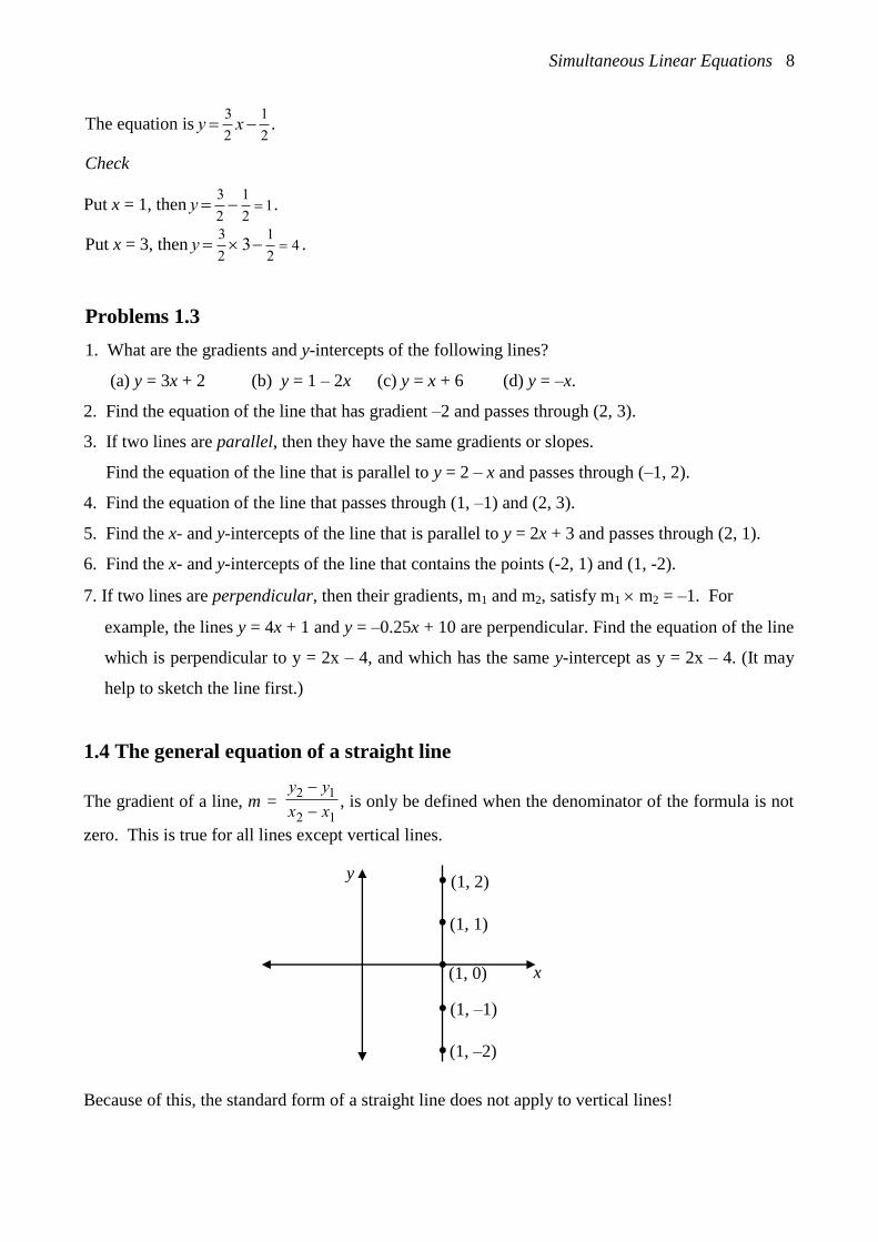
1.4 The general equation of a straight line

The gradient of a line, m =

y2 y1

x2 x1, is only be defined when the denominator of the formula is not

zero. This is true for all lines except vertical lines.

Because of this, the standard form of a straight line does not apply to vertical lines!

(1, 1)

•

•

•

• (1, 0) x

y • (1, 2)

(1, –1)

(1, –2)

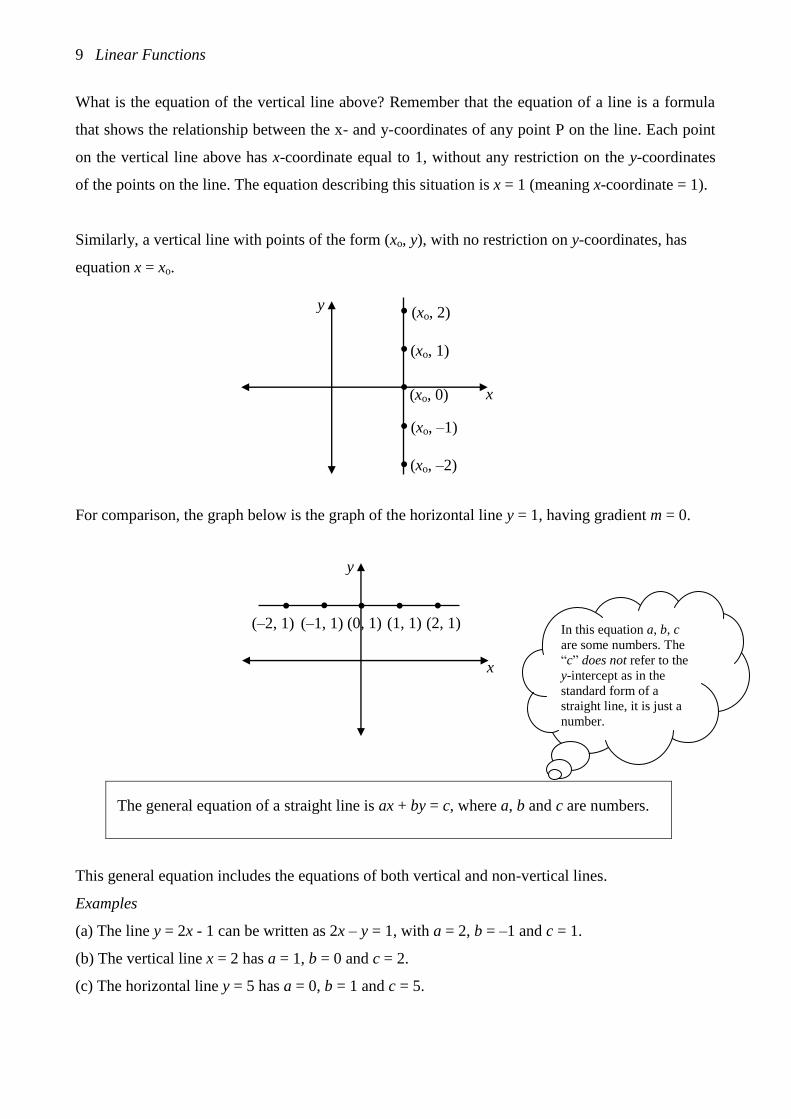
9 Linear Functions

What is the equation of the vertical line above? Remember that the equation of a line is a formula

that shows the relationship between the x- and y-coordinates of any point P on the line. Each point

on the vertical line above has x-coordinate equal to 1, without any restriction on the y-coordinates

of the points on the line. The equation describing this situation is x = 1 (meaning x-coordinate = 1).

Similarly, a vertical line with points of the form (xo, y), with no restriction on y-coordinates, has

equation x = xo.

For comparison, the graph below is the graph of the horizontal line y = 1, having gradient m = 0.

The general equation of a straight line is ax + by = c, where a, b and c are numbers.

This general equation includes the equations of both vertical and non-vertical lines.

Examples

(a) The line y = 2x - 1 can be written as 2x – y = 1, with a = 2, b = –1 and c = 1.

(b) The vertical line x = 2 has a = 1, b = 0 and c = 2.

(c) The horizontal line y = 5 has a = 0, b = 1 and c = 5.

In this equation a, b, c

are some numbers. The

“c” does not refer to the

y-intercept as in the

standard form of a

straight line, it is just a

number.

(xo, 1)

•

•

•

• (xo, 0) x

y • (xo, 2)

(xo, –1)

(xo, –2)

(0, 1) (1, 1)

x

y

• • • • • (2, 1) (–1, 1) (–2, 1)


It is easy to calculate the intercepts of a straight line from its general equation . . .

Example

Find the intercepts of the line 2x + 3y = 12

Answer

Put y = 0, then

2x 12 x 6.

Put x = 0, then

3y12 y 4 .

The intercepts are (6, 0) and (0, 4).

. . . however, to find the gradient of a line, you need to change its equation into the standard form.

Example

Find the gradient of 2x + 3y = 12

Answer

2x 3y 12

3y 2x12

y 2

3x 4

The gradient is m =

2

3.

2 Simultaneous Linear Equations

11

It is often useful to find the point of intersection of two straight lines.

Example

A company manufactures seat covers. It leases workspace at a fixed monthly cost of $ 2 000. Each

seat cover costs $15 to make (materials and labour). If x seat covers were made each month, the

total monthly cost (C) would be given by the cost function:

C = 2 000 + 15x (dollars)

Each seat cover will be sold for $22.50. The total income from sales (I) is given by the income

function:

I = 22.5x (dollars),

where x is the number of seat covers sold.

The graphs of the cost and income functions are drawn below using the same axes. The point of

intersection of the two lines corresponds to the breakeven point, where income equals cost.

Two non-parallel lines have only one point of intersection, and the coordinates of this point can be

estimated using a graph. Alternatively, the coordinates can be found exactly by using algebra to

solve a pair of simultaneous linear equations.

(267, 6 000)

100 200 300 0

2000

4000

6000

Number of Seat Covers

Am

ou

nt

($)

I = 22.5x

C = 2 000 + 15x

•


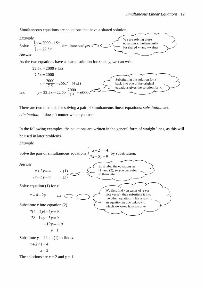
Simultaneous equations are equations that have a shared solution.

Example

Solve

y 200015x

y 22.5x

simultaneously.

Answer

As the two equations have a shared solution for x and y, we can write

22.5x 200015x

7.5x 2000

x 2000

7.5 266.7 (4 sf)

and

y 22.5x 22.52000

7.5 6000 .

There are two methods for solving a pair of simultaneous linear equations: substitution and

elimination. It doesn’t matter which you use.

In the following examples, the equations are written in the general form of straight lines, as this will

be used in later problems.

Example

Solve the pair of simultaneous equations

x2y 4

7x 5y 9

by substitution.

Answer

x2y 4 (1)

7x 5y 9 (2)

Solve equation (1) for x

x 42y

Substitute x into equation (2)

7(4 – 2y) 5y 9

2814y 5y 9

19y 19

y 1

Substitute y = 1 into (1) to find x.

x21 4

x 2

The solutions are x = 2 and y = 1.

First label the equations as

(1) and (2), so you can refer

to them later

We first find x in terms of y (or

vice versa), then substitute it into

the other equation. This results in

an equation in one unknown,

which we know how to solve.

We are solving these

equations simultaneously

for shared x- and y-values.

Substituting the solution for x

back into one of the original

equations gives the solution for y.

13 Linear Functions

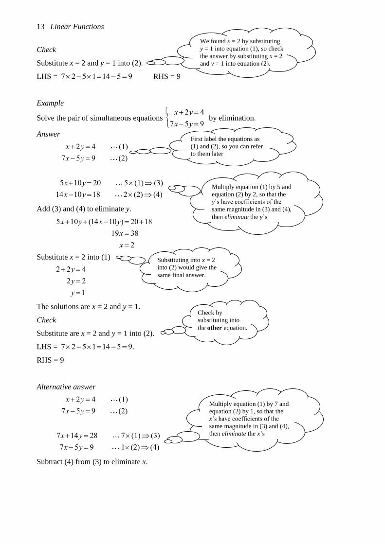
Check

Substitute x = 2 and y = 1 into (2).

LHS =

72511459 RHS = 9

Example

Solve the pair of simultaneous equations

x2y 4

7x 5y 9

by elimination.

Answer

x2y 4 (1)

7x 5y 9 (2)

5x10y 20 5 (1) (3)

14x 10y 18 2 (2) (4)

Add (3) and (4) to eliminate y.

5x10y (14x 10y) 2018

19x 38

x 2

Substitute x = 2 into (1)

2 2y 4

2y 2

y 1


Check

Substitute are x = 2 and y = 1 into (2).

LHS =

72511459.

RHS = 9

Alternative answer

x2y 4 (1)

7x 5y 9 (2)

7x14y 28 7 (1) (3)

7x5y 9 1 (2) (4)

Subtract (4) from (3) to eliminate x.

First label the equations as

(1) and (2), so you can refer

to them later

Check by

substituting into

the other equation.

Multiply equation (1) by 5 and

equation (2) by 2, so that the

y’s have coefficients of the

same magnitude in (3) and (4),

then eliminate the y’s

Substituting into x = 2

into (2) would give the

same final answer.

Multiply equation (1) by 7 and

equation (2) by 1, so that the

x’s have coefficients of the

same magnitude in (3) and (4),

then eliminate the x’s

We found x = 2 by substituting

y = 1 into equation (1), so check

the answer by substituting x = 2

and y = 1 into equation (2).


7x14y (7x 5y) 289

19y 19

y 1

Substitute y = 1 into (1)

x 2 4

x 2


Problems 2

Solve the following pairs of simultaneous equations

(a) 2x y 12

2x y 8

(b) x2y 6

x5y 18

(c) 2x y 4

4x y 10

(d) 2x y 22

3x 2y 5

(e) x 3y 8

3x y 4

(f) 3x 4y 7

2x5y 3

Check as

before.

Substituting y = 1 into

(2) would give the same

final answer.

3 Linear Inequalities

15

The inequality y 2x 1 is an example of a linear inequality. The graph of this inequality is the set

of all points in the shaded region below. This can be written as {(x, y) : y 2x 1}.

To graph this linear inequality, we first draw the line y = 2x – 1. This line has the intercepts (0.5, 1)

and (0, –1) and is shown below.

1 –1 0

1

–1

y

x

y < 2x – 1

1 –1 0

1

–1

y

x

•

•

• (1, –1)

(1, y)

(1, 1)

y = 2x – 1

Linear Inequalities 16

Now look at the vertical line x = 1 on the graph. Begin at the point (1, –1). The x- and y-

coordinates of this point satisfy the inequality y 2x 1 as 12 11. Now move slowly

upwards along the line x = 1. As you move upwards, the y-coordinate of the point (1, y) will

increase. Eventually you will reach the line y = 2x – 1 at the point (1, 1). The x- and y-coordinates

of this point satisfy the equation y = 2x – 1. Before we reach the line y = 2x – 1, the x- and y-

coordinates of each point on x = 1 satisfied the inequality

y 2x1 (because the value of y has

been increasing as we moved upwards). Now continue moving upwards along line x = 1. The y-

coordinate of the point (1, y) will continue to increase. After you cross over the line y = 2x – 1, you

can see that the x- and y-coordinates of each point on x = 1 will satisfy the inequality

y 2x1.

This shows that all the points on line x = 1 and below y = 2x – 1 satisfy

y 2x1, and that all

points on line x = 1 and above y = 2x – 1, satisfy

y 2x1.

We can repeat this, beginning at any point on any vertical line. Each will show that the line y = 2x –

1 divides the plane into 2 regions, and that points in the region below the line satisfy

y 2x1 and

all points in the region above satisfy

y 2x1. The line y = 2x – 1 is drawn with a dashed line in

the graph of

y 2x1 to show that the points on the line do not satisfy

y 2x1.

Examples

a

y

x

x ≤ a

a

y

x

y > a

y = mx + c

y

x

y ≥ mx + c

y < mx + c

y = mx + c

y

x

17 Linear Functions

A straight line divides the coordinate plane into two regions, one below the line and one above it. If

you are not sure which region satisfies a linear inequality, just select a point in one region and check

if it satisfies the inequality.

Example

Sketch the region satisfying

2x3y 6.

Answer

Put y = 0, then

2x 6 x 3.

Put x = 0, then

3y 6 y2 .

The intercepts of 2x – 3y = 6 are (3, 0) and (0, –2).

Example

A person on a certain diet should have less than 300 mg of cholesterol per day. It is known that 1

gm of whole egg contains 6.6 mg of cholesterol and 1 gm of liver contains 3.6 mg of cholesterol.

Find the relationship between the quantities of egg and liver that can be allowed in the diet,

assuming that these are the main sources of cholesterol. Draw a graph showing this relationship.

Answer

(a) The relationship.

If x gm of egg and y gm of liver is eaten, then the amount of cholesterol will be 6.6x + 3.6y. This

has to be less than 300, so the relationship between the quantities of egg and liver allowed in the

diet is 6.6x + 3.6y < 300.

(b) The graph of 6.6x + 3.6y < 300.

Put x = 0, then

3.6y 300 y 300

3.6 83.

2x – 3y > 6

2x – 3y =

6

y

x 3

–2

The point (4, 0) is

below the line, and

also satisfies the

inequality, so all points

below the line satisfy

the inequality.

First draw the line which

splits the plane into two

regions, then decide

which region satisfies the

inequality.

Use a dashed line, as

points on the line don’t

satisfy the inequality

Linear Inequalities 18

Put y = 0, then

6.6x 300 x 300

6.6 45.

The intercepts are (45, 0) and (0, 83).

Example

Solve the simultaneous linear inequalities below graphically.

x y 2

y x 1

x 0

y 0

Answer

45

83

y

x 100

100

0

As the amount of eggs

and liver can’t be

negative, we must

have x ≥ 0 and y ≥ 0.

y

x 2

2

0 1

(1.5, 0.5)

x + y = 2

y = x – 1

19 Linear Functions

Problems 3

1. Sketch the graphs of the following inequalities.

(a) y > 1 – x (b) 2x – y ≤ 4 (c) 3x ≥ y – 6

2. Solve the simultaneous linear inequalities below graphically.

x y 2

3x y 3

3(a) A laboratory needs at least 300 beakers of one size and at least 400 beakers of a second size. It

is decided that the total number of beakers should be less than 1200. Draw a graph showing the

possible numbers of each kind of beaker.

3(b) Each beaker of the first size needs 45 sq cm of shelf space, and each beaker of the second size

needs 30 sq cm of shelf space. However, there is only 4 sq m of shelf space. Draw a graph showing

the possible numbers of each kind of beaker.

A Appendix: Linear Equations

20

A linear equation is an equation like 2x – 3 = 12. This refresher consists of a series of examples

showing how to solve these equations.

The general principle for solving all linear equations is to rearrange the equation so that the

unknown is on the left hand side and a number is on the right hand side.

Example

Solve x – 3 = 0

Answer

Add 3 to both sides of the equation:

x 3 0

x 3 3 0 3

x 3

Example

Solve w + 10 = 0

Answer

Subtract 10 from both sides of the equation:

w10 0

w1010 010

w 10

Example

Solve 2s + 10 = 0

Answer

2s 10 0

2s 10

s 5

Always carry out the same action

on both sides of the equation.

Some of these steps don’t

need to be written down.

Rearrange the equation with a

multiple of the unknown on the

LHS, and a number on the RHS.

Then divide both

sides by 2 to get s

by itself.

Linear Equations Refresher 21

Example

Solve 032

x

Answer

6

322

2

032

x

x

x

Example

Solve 3w 10 4w 12 3(1w)

Answer

2

5

52

15102

15103

15103

33124103

)1(3124103

w

w

w

wwww

ww

www

www

Example

Solve

3

x1 2 .

Answer

3

x1 2

(x1)3

x1 (x1) 2

3 2(x1)

3 2x 2

1 2x

2x 1

x 1

2

Multiply both sides by 2 to get

x by itself.

First expand brackets and

simplify each side.

Unknowns on the LHS,

numbers on the RHS.

Remove the denominator on the LHS

by multiplying both sides by x + 1.

Interchange the LHS and RHS

to get the unknown on the LHS.

Answers 1

C Appendix: Answers

Section 1.1

0.5

–1

x

(a) y

0.5

–0.1

x

(c) y

0.5

–10

x

(b) y

1

3

x

(d, e, f)

0

2

1 y = x

y = 2x

y = 3x y

1

1

x

(g) f(x)

–0.5

–1

x

(h) f(x)

2/3

2

x

(i) g(x)

2 Linear Functions

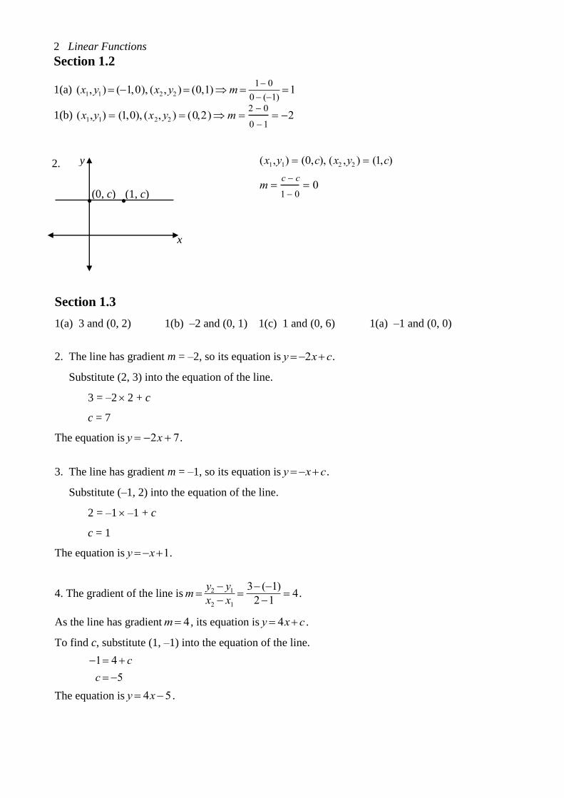
Section 1.2

1(a)

(x1,y1) (1,0), (x2, y2 ) (0,1)m 1 0

0 (1)1

1(b) (x1,y1) (1,0), (x2, y2 ) (0,2) m 2 0

0 1 2

(x1,y1) (0,c), (x2 ,y2 ) (1,c)

m c c

1 0 0

Section 1.3

1(a) 3 and (0, 2) 1(b) –2 and (0, 1) 1(c) 1 and (0, 6) 1(a) –1 and (0, 0)

2. The line has gradient m = –2, so its equation is

y 2xc.

Substitute (2, 3) into the equation of the line.

3 = –2 2 + c

c = 7

The equation is y 2x 7.

3. The line has gradient m = –1, so its equation is

yxc.

Substitute (–1, 2) into the equation of the line.

2 = –1 –1 + c

c = 1

The equation is

y x1.

4. The gradient of the line is

m y2 y1x2 x1

3 (1)

21 4.


m 4 , its equation is

y 4xc .

To find c, substitute (1, –1) into the equation of the line.

1 4 c

c 5

The equation is

y 4x5 .

(0, c) (1, c)

x

y 2.

• •

Answers 3

5. The line has gradient m = 2, so its equation is

y 2xc.

Substitute (2, 1) into the equation of the line.

1 2 2 c

c 3

The y-intercept is (0, –3), and the equation is

y 2x 3.

Put y = 0 in 2/332 xxy , so the x-intercept is (3/2, 0).


m y2 y1x2 x1

21

1 (2)1.


m1, its equation is

yxc.

To find c, substitute (-2, 1) into the equation of the line.

1 (2) c

c 1

The y-intercept is (0, –1), and the equation is y x 1.

Put y = 0 in y x 1 x 1, so the x-intercept is (–1, 0).


m 1

2 and the y-intercept is (0, –4). The equation is

y 1

2x 4 .

Section 2

These questions can be answered in more than one way.

(a) 2x y 12 (1)

2x y 8 (2)

Solve equation (1) for y

y 122x

Substitute y into equation (2)

2x (12 - 2x) 8

4x 12 8

x 5

Substitute x = 5 into (1).

10 y 12

y 2


(b) x2y 6 (1)

x5y 18 (2)

Solve equation (1) for x

x 6 - 2y


6 - 2y 5y 18

3y 12

y 4


x8 6

x 2

The solutions are x = –2 and y = 4.

4 Linear Functions

(c) 2x y 4 (1)

4x y 10 (2)

Solve equation (1) for y

y 2x4


4x (2x 4)10

2x 4 10

x 3


12 y 10

y 2


(d) 2x y 22 (1)

3x 2y 5 (2)

4x 2y 44 2 (1) (3)

3x 2y 5 (2) (4)


4x2y (3x 2y) 44 5

7x 49

x 7


14 y 22

y 8


(e) x 3y 8 (1)

3x y 4 (2)

x 3y 8 (1) (3)

9x 3y 12 3 (2) (4)


x 3y (9x 3y) 812

10x 20

x 2


2 3y 8

y 2


(f) 3x 4y 7 (1)

2x 5y 3 (2)

6x 8y 14 2 (1) (3)

6x15y 9 3 (2) (4)

Subtract (3) from (4) to eliminate x.

6x15y (6x 8y) 914

23y 23

y 1

Substitute y = -1 into (1)

3x 4 (1) 7

3x 4 7

x 1

The solutions are x = 1 and y = -1.

Answers 5

Section 3

3(a) If the laboratory obtained x beakers of the first size and y beakers of the second size, then

we should have x ≥ 300, y ≥ 400 and x + y ≤ 1200. The shaded area below shows the graph of

these inequalities.

2

y

x

2

2.

y

x 1200

1200

0

x = 300

y = 400

x + y = 1200

1

y

x

1

1(a)

2

y

x

–4

1(b)

–2

y

x

6

1(c)

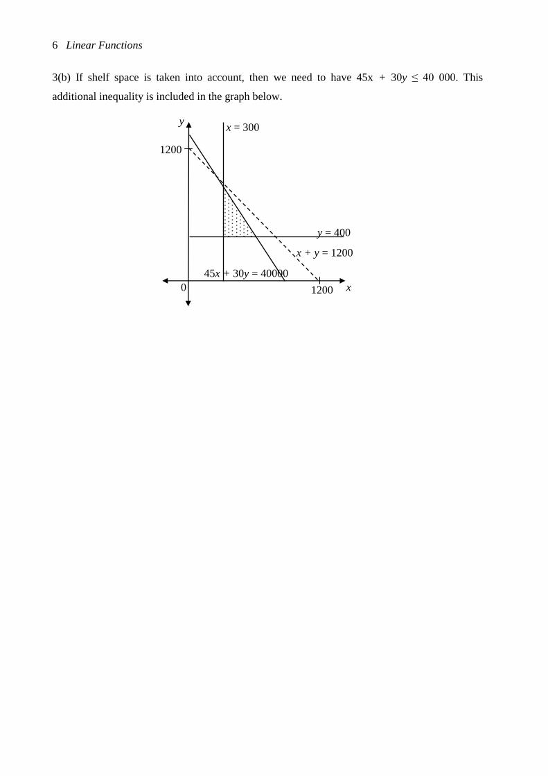
6 Linear Functions

3(b) If shelf space is taken into account, then we need to have 45x + 30y ≤ 40 000. This

additional inequality is included in the graph below.

889

y

x 1200

1200

0

x = 300

y = 400

x + y = 1200

1333

45x + 30y = 40000

Topic 2 Linear Functions - University of Adelaide · Topic 2 Linear Functions –1 0 x 1 –1 y y <...

Documents

Transcript of Topic 2 Linear Functions - University of Adelaide · Topic 2 Linear Functions –1 0 x 1 –1 y y <...