Topic 2 : Diﬁraction

Diffraction Session: 2009-2010 -1

Topic 2 : Diffraction

2.1 Introduction

So far we have considered a range of models for light, each one appropriate to the phe-nomena we are considering. The models so far have always taken the direction of thepropagation to be given by Snell’s Law, so that it only changes at refractive index bound-aries.

To go further we need to consider the spatial wave nature of light, which results indiffraction. In this course we will consider a simplified scalar model where we will ignorethe polarisation effects of light.

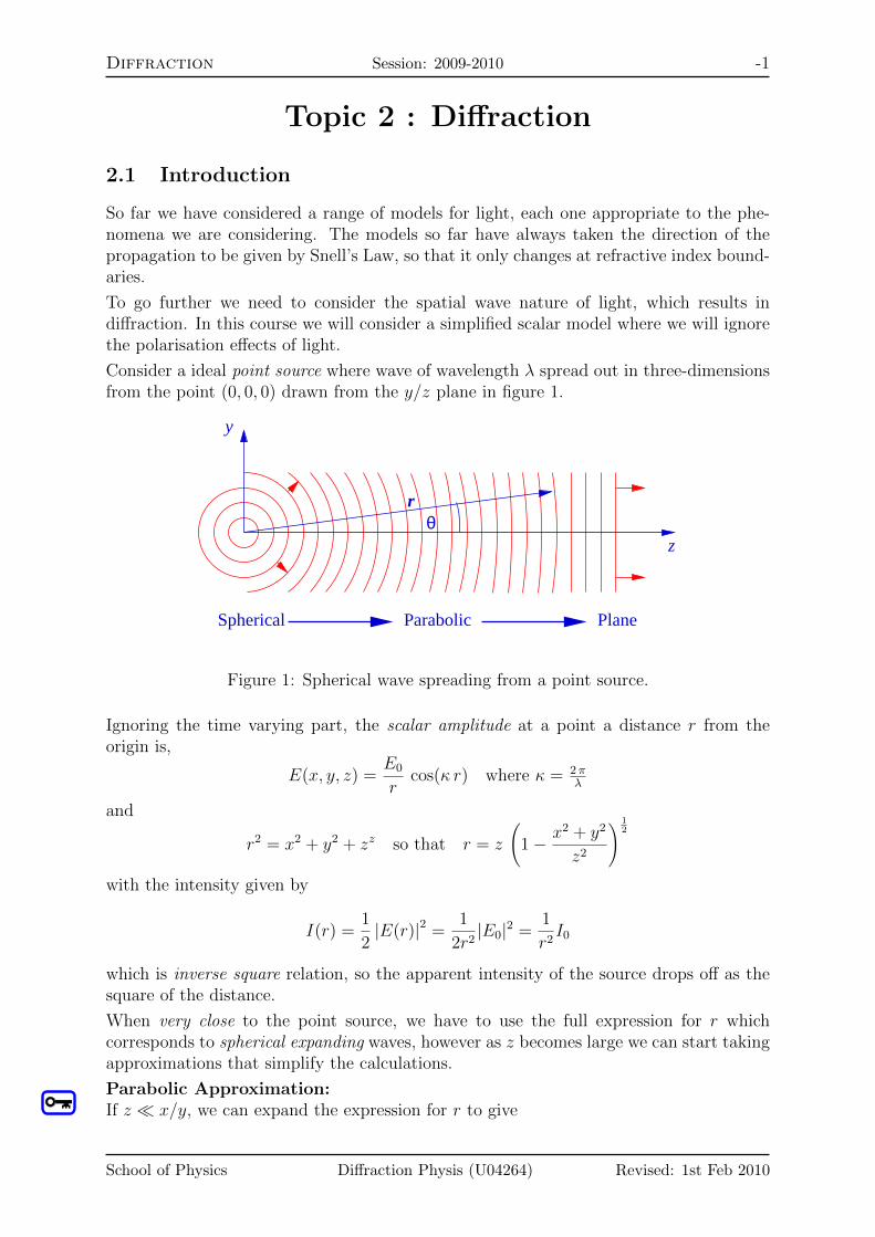
Consider a ideal point source where wave of wavelength λ spread out in three-dimensionsfrom the point (0, 0, 0) drawn from the y/z plane in figure 1.

Spherical Parabolic Plane

θz

y

r

Figure 1: Spherical wave spreading from a point source.

Ignoring the time varying part, the scalar amplitude at a point a distance r from theorigin is,

E(x, y, z) =E0

rcos(κ r) where κ = 2π

λ

and

r2 = x2 + y2 + zz so that r = z

(1− x2 + y2

z2

) 12

with the intensity given by

I(r) =1

2|E(r)|2 = 1

2r2|E0|2 = 1

r2I0

which is inverse square relation, so the apparent intensity of the source drops off as thesquare of the distance.

When very close to the point source, we have to use the full expression for r whichcorresponds to spherical expanding waves, however as z becomes large we can start takingapproximations that simplify the calculations.

Parabolic Approximation:If z ¿ x/y, we can expand the expression for r to give

School of Physics Diffraction Physis (U04264) Revised: 1st Feb 2010


r = z +x2 + y2

2z

which corresponds to parabolic wave approximation, which will result in Fresnel or nearfield diffraction.

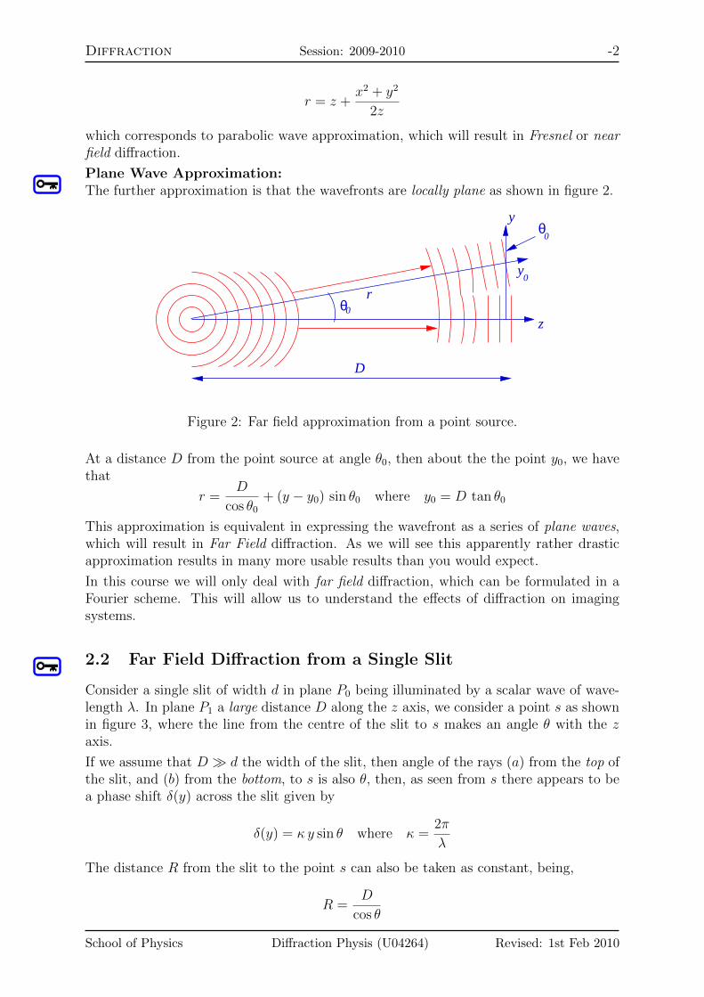
Plane Wave Approximation:The further approximation is that the wavefronts are locally plane as shown in figure 2.

θz

D

r0

y0

yθ

0

Figure 2: Far field approximation from a point source.

At a distance D from the point source at angle θ0, then about the the point y0, we havethat

r =D

cos θ0+ (y − y0) sin θ0 where y0 = D tan θ0

This approximation is equivalent in expressing the wavefront as a series of plane waves,which will result in Far Field diffraction. As we will see this apparently rather drasticapproximation results in many more usable results than you would expect.

In this course we will only deal with far field diffraction, which can be formulated in aFourier scheme. This will allow us to understand the effects of diffraction on imagingsystems.

2.2 Far Field Diffraction from a Single Slit

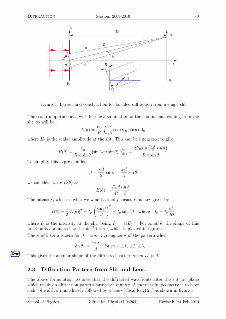
Consider a single slit of width d in plane P0 being illuminated by a scalar wave of wave-length λ. In plane P1 a large distance D along the z axis, we consider a point s as shownin figure 3, where the line from the centre of the slit to s makes an angle θ with the zaxis.

If we assume that D À d the width of the slit, then angle of the rays (a) from the top ofthe slit, and (b) from the bottom, to s is also θ, then, as seen from s there appears to bea phase shift δ(y) across the slit given by

δ(y) = κ y sin θ where κ =2π

λ

The distance R from the slit to the point s can also be taken as constant, being,

R =D

cos θ



d

y

z

θ

δ

θ

D

PP

s

01

(a)

(b)

R

Figure 3: Layout and construction for far-filed diffraction from a single slit

The scalar amplitude at s will then be a summation of the components coming from theslit, so will be,

E(θ) =E0

R

∫ d/2

−d/2cos (κ y sin θ) dy

where E0 is the scalar amplitude at the slit. This can be integrated to give

E(θ) =E0

Rκ sin θ|sin (κ y sin θ)|d/2−d/2 =

2E0 sin(κ d2

sin θ)

Rκ sin θ

To simplify this expression let

β =κ d

2sin θ =

π d

λsin θ

we can then write E(θ) as

E(θ) =E0 d

R

sin β

β

The intensity, which is what we would actually measure, is now given by

I(θ) =1

2|E(θ)|2 = Ip

(sin β

β

)2

= Ip sinc2β where Ip = I0

d2

R2

where I0 is the intensity at the slit, being I0 = 12|E0|2. For small θ, the shape of this

function is dominated by the sinc2β term, which is plotted in figure 4.

The sinc2β term is zero for β = ±mπ, giving zeros of the pattern when

sin θm =mλ

dfor m = ±1, ±2, ±3, · · ·

This gives the angular shape of the diffracted pattern when D À d.

2.3 Diffraction Pattern from Slit and Lens

The above formulation assumes that the diffracted wavefronts after the slit are planewhich result on diffraction pattern formed at infinity. A more useful geometry is to havea slit of width d immediately followed by a lens of focal length f as shown in figure 5.



0

0.1

0.2

0.3

0.4

0.5

0.6

0.7

0.8

0.9

1

-10 -5 0 5 10

sinc(x)**2

Figure 4: Shape of sinc2(x)

d

y

P0

z

θ

P P

s

θ

bfb

f

w

Figure 5: Diffraction from a slit imaged by a lens

We know from previous that a collimated beam at angle θ striking the front of the lensare images to a point in the back focal plane Pfb , which is a distance f from the backprincipal plane of the lens. Thus a plane wave, diffracted in direction θ will be focusedas s, where

s = f tan θ ≈ f θ for small θ

so the intensity in the back focal plane will be,

I(s) = Ipsinc2

(π d

λ fs

)

which has zeros at

sm = mλf

dfor m = ±1, ±2, ±3, · · ·

so having a width, being the distance between the ±1 zeros, of

w =2λ f

d



Note the reciprocal relations between d and w, as as the slit get narrower then it diffrac-tion pattern gets wider.

2.4 The Fourier Approach

The Fourier transform1 of a function f(x) is given by,

F (u) = F {f(x)} =∫ ∞

−∞f(x) exp(−i 2π ux) dx

which for a real function f(x) we can write as

F (u) =∫ ∞

−∞f(x) cos(2π ux) dx− i

∫ ∞

−∞f(x) sin(2π ux) dx

If we now define a function p(x) which represents the slit being,

p(x) = 1 for |x| < d/2

= 0 else

then from previous we can write that,

E(θ) =E0

R

∫ ∞

−∞p(y) cos(κy sin θ) dy =

E0

RR{P (κ sin θ)} where κ =

2π

λ

where P (u) = F {p(x)}, or more importantly, if we have a lens of focal length f after theslit, then in the back focal plane of the lens we have

E(s) =E0

f

∫ ∞

−∞p(y) cos

(2π

λ fys

)dy =

E0

fR

{P

(1

λ fs

)}

and the intensity,

I(s) = I0

∣∣∣∣∣P(

s

λ f

)∣∣∣∣∣2

so we have the important result that the intensity in the back focal plane is the modulussquared of the scaled Fourier transform of p(x), which represents the slit. It is easy toshow that F {p(x)} is given by

P (u) = dsinc(π d u)

where d is the the width of the slit.

The scheme is easily extended to a two-dimensional slit, being a rectangle of sides a× b,by defining a rectangle function,

p(x, y) = 1 when |x| < a/2 and |y| < b/2

= 0 else

The two-dimensional Fourier transform is given by

P (u, v) = a b sinc(π a u) sinc(π b v)

1See The Fourier Transform, (What you need to know), for detail.



since both the Fourier transform and p(x, y) is separable. Then following the abovescheme the intensity diffracted from a rectangle, in the back focal plane of a lens of focallength f is given by

I(s, t) = I0 sinc2

(π a s

λ f

)sinc2

(π b t

λ f

)

where I0 is the intensity at the centre of the pattern. This shape is plotted as a surfaceplot in figure 6, for for an aperture where a = 3 b showing two sinc() at right angles,one being the three times wider than the other. The log() of the function is also plottedwhich makes the structure much more obvious.

-8-6

-4-2

0 2

4 6

8 -8-6

-4-2

0 2

4 6

8

0 1 2 3 4 5 6 7 8 9

-8-6

-4-2

0 2

4 6

8 -8-6

-4-2

0 2

4 6

8

-7-6-5-4-3-2-1 0 1 2 3

Figure 6: Plot of diffraction pattern from a rectangular aperture with of size a× b wherea = 3 b, and its log().

2.5 Diffraction from Two Slits

The power of the Fourier approach really become obvious when the diffracting objectbecome more complex. Consider diffraction from two slits of width a separated by b. If,as above, we define p(x) to be the transmission function for one slit, being given by

p(x) = 1 for |x| < a/2

= 0 else

then two slits, separated by b can be written as

f(x) = p(x) ¯[δ

(x− b

2

)+ δ

(x+

b

2

)]

where δ(x) is the δ−function, and ¯ is the convolution operator. This is shown schemat-ically in figure 7.

We then know from the convolution theorem, that the Fourier transform is just the prod-uct of the Fourier transform of the two function, so in this case we get that

F (u) = sinc(π a u) cos(π b u)



a a a

b

=

b

b/2

p(x)

Figure 7: Representation of two slits by convolution.

The diffracted intensity behind a lens of focal length f is now just

I(s) = I0 sinc2

(π a

λfs

)cos2

(π b

λfs

)

where I0 is the intensity at the centre of the pattern. A plot of this intensity for b = 6ais shown in figure 8, along with a log() plot to make the outer peaks more visible.

0

0.1

0.2

0.3

0.4

0.5

0.6

0.7

0.8

0.9

1

-10 -5 0 5 10

Inte

nsity

Distance

-5

-4.5

-4

-3.5

-3

-2.5

-2

-1.5

-1

-0.5

0

0.5

-10 -5 0 5 10

Inte

nsity

Distance

Figure 8: Plot of intensity diffracted from two slits separated by six times their width,and its log().

The shape is cos() fringes from the two slits, exactly as seen in workshop question 7.1, butmodulated by the sinc2() resulting from the finite thickness of the slits. If you comparethis analysis with the traditional scheme in the textbooks, the power of the Fouriertechniques is obvious!

2.6 The Diffraction Grating

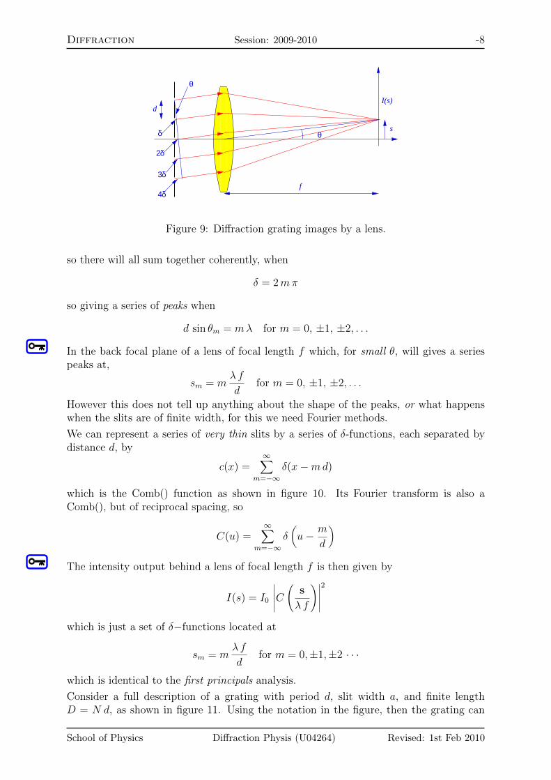
The diffraction grating in a series of thin slits all separated by a distance d, which isimages by a lens of focal length f as shown in figure 9. The traditional and simpleanalysis is that at angle θ, the phase delay between light diffracted from adjacent slits is,

δ =2π

λd sinθ



s

f

d

θ

θ

3δ

4δ

2δ

δ

I(s)

Figure 9: Diffraction grating images by a lens.

so there will all sum together coherently, when

δ = 2mπ

so giving a series of peaks when

d sin θm = mλ for m = 0, ±1, ±2, . . .

In the back focal plane of a lens of focal length f which, for small θ, will gives a seriespeaks at,

sm = mλf

dfor m = 0, ±1, ±2, . . .

However this does not tell up anything about the shape of the peaks, or what happenswhen the slits are of finite width, for this we need Fourier methods.

We can represent a series of very thin slits by a series of δ-functions, each separated bydistance d, by

c(x) =∞∑

m=−∞δ(x−md)

which is the Comb() function as shown in figure 10. Its Fourier transform is also aComb(), but of reciprocal spacing, so

C(u) =∞∑

m=−∞δ(u− m

d

)

The intensity output behind a lens of focal length f is then given by

I(s) = I0

∣∣∣∣∣C(

s

λ f

)∣∣∣∣∣2

which is just a set of δ−functions located at

sm = mλf

dfor m = 0,±1,±2 · · ·

which is identical to the first principals analysis.

Consider a full description of a grating with period d, slit width a, and finite lengthD = N d, as shown in figure 11. Using the notation in the figure, then the grating can



x

u

0

0

x

1/ x

∆

∆

Figure 10: A Comb() function and its Fourier Transform.

a

a

d

D = N d D = N d

=x

d

w(x)p(x)c(x)

Figure 11: Full description of a grating of period d, slit width a and finite extend D = N d

be described by a function,

f(x) = {c(x)¯ p(x)} w(x)

which again from the convolution theorem, has Fourier transform

F (u) = {W (u)¯ C(u)} P (u)

where

C(u) =∞∑

m=−∞δ(u− m

d

), P (u) = sinc(πa u) and W (u) = sinc(πN du)

The intensity is then just,

I(s) = I0

∣∣∣∣∣F(

s

λ f

)∣∣∣∣∣2

which is plotted for a = 1, d = 5 and N = 10, which shows a series of sharp sinc2()functions separated by a constant distance and weighted by an overall sinc2().

2.6.1 The Grating Spectrometer

In the grating spectrometer a collimated beam containing multiple wavelengths strikesa diffraction grating and is diffracted to form ±-order diffracted spectra as shown in



0

0.1

0.2

0.3

0.4

0.5

0.6

0.7

0.8

0.9

1

-0.4 -0.2 0 0.2 0.4

Figure 12: Output of a grating of period d, slit width a and finite extend D = N d

Slit

Collimated beamGrating

D d+1 order

−1 order

ff

Figure 13: Layout of basic grating spectrometer.

figure 13. In practical systems the imaging lens system can rotate about the centre ofthe grating so that the angle of the diffracted image of the slit can be measured.

Consider the system being illuminated with two wavelength λ1 and λ2, then at the mth

order diffraction pattern we two sinc2() peaks as shown in figure 14. This position of thecentre of the two peaks will be at

s1 =mλ1 f

dand s2 =

mλ2 f

d

where d is the grating spacing, and f is the effective focal length of the spectrometerimaging system. Their separation will therefore be

δs =mδ λ f

dwhere δλ = λ1 − λ2

Each peak is a sinc2(), and if we assume that λ1 ≈ λ2 then both peaks have the samewidth, with their first zero at a distance

∆s =λ0 f

Dwhere λ0 =

1

2(λ1 + λ2)



λ λ

s s

δ s

∆ ss

1

1 2

2

Figure 14: Diffraction from source with two wavelengths.

We get

1. δλ is large, then δs À ∆s, so the two peaks are well separated, and hence resolved,

2. δλ is small the two peaks start of overlap, and finally merge to one as δλ → 0, andhence not resolved.

We say that the two peaks are just resolved when δs = ∆s, so that the centre of one peakis at the first zero of the other. This is shown in figure 15, showing at this criteria thereis a valley of about 20% of the peak height.

0

0.1

0.2

0.3

0.4

0.5

0.6

0.7

0.8

0.9

1

-3 -2 -1 0 1 2 3

Figure 15: Two sinc2() peaks at their resolution limit

This sets a limit of the smallest δλ we can resolve with this instrument where

λ0

δλ=

mD

d= mN

where N is the number of lines on the grating, and λ0 is the average wavelength and m is



the diffraction order. Therefore to get a good resolution we been a grating large gratingwith many lines, and ideally use as high an order as possible. See workshop question ??for a numerical example.

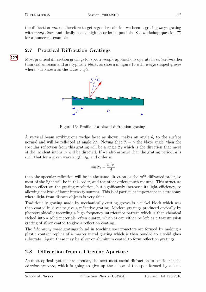
2.7 Practical Diffraction Gratings

Most practical diffraction gratings for spectroscopic applications operate in reflectionrather???

than transmission and are typically blazed as shown in figure 16 with wedge shaped groveswhere γ is known as the blaze angle.

d

γ

D

θ θi i

Figure 16: Profile of a blazed diffraction grating.

A vertical beam striking one wedge facet as shown, makes an angle θi to the surfacenormal and will be reflected at angle 2θi. Noting that θi = γ the blaze angle, then thespecular reflection from this grating will be a angle 2γ which is the direction that mostof the incident intensity will be directed. If we also arrange that the grating period, d issuch that for a given wavelength λ0, and order m

sin 2γ =mλ0

d

then the specular reflection will be in the same direction as the mth diffracted order, somost of the light will be in this order, and the other orders much reduces. This structurehas no effect on the grating resolution, but significantly increases its light efficiency, soallowing analysis of lower intensity sources. This is of particular importance in astronomywhere light from distant objects is very faint.

Traditionally grating made by mechanically cutting groves is a nickel block which wasthen coated in silver to give a reflective grating. Modern gratings produced optically byphotographically recording a high frequency interference pattern which is then chemicaletched into a solid materials, often quartz, which is can either be left as a transmissiongrating of silver coated to give a reflection coating.

The laboratory grade gratings found in teaching spectrometers are formed by making aplastic contact replica of a master metal grating which is then bonded to a solid glasssubstrate. Again these may be silver or aluminum coated to form reflection gratings.

2.8 Diffraction from a Circular Aperture

As most optical systems are circular, the next most useful diffraction to consider is thecircular aperture, which is going to give up the shape of the spot formed by a lens.



Consider the circular aperture of radius a, being defined by,

p(x, y) = 1 when x2 + y2 ≤ a2

= 0 else

First we need to calculate the Fourier transform P (u, v), which using

x = ρ cos θ y = ρ, sin θ

we have that

P (u, v) =∫ a

0

∫ 2π

0exp (−i 2π(u ρ cos θ + v ρ sin θ)) ρ dρ dθ

where the limits of integration are across a circle of radius a. The circular aperture p(x, y)is clearly circularly symmetric, so it Fourier transform must also be circular symmetric.Therefore we only been th calculate P (u, v) along one radial line, select the line withv = 0, to give

P (u, 0) =∫ a

0

∫ 2π

0exp (−i 2π u ρ cos θ) ρ dρ dθ

Now from Physical Mathematics we have the standard identity that∫ 2π

0exp(i r cos θ) dθ = 2πJ0(r)

where J0(ρ) is the zero order Bessel function, we get that

P (u, 0) = 2π∫ a

0J0(2π u ρ) ρ dρ

We now need the second identity that

r J0(r) =d

d r(r J1(r)) so that

∫ r

0J0(t) t dt = r J1(r)

so if we let t = 2π u ρ, we get that

P (u, 0) =1

2π

∫ 2πua

0J0(t)

1

u2t dt

which we can then integrate to get

P (u, 0) =2π u a

u2J1(2π u a) = 4π2 a2

J1(2π u a)

2π u a

using that it is circularly symmetric, we can then write this in two dimensions as

P (u, v) = 4π2 a2J1(2π aw)

2π awwhere w2 = u2 + v2

We then know from above that the intensity in the back focal plane of a lens of focallength f , is the square modulus of the Fourier transform scaled by λ f , so giving,

I(s, t) = 4I0

∣∣∣∣∣∣J1

(2πλf

a r)

2πλf

a r

∣∣∣∣∣∣

2

where r2 = s2 + t2

where we have incorporated the various constants into I0, and is the intensity at thecentre of the pattern.

To analyse this we need to consider the shape of the J1(x)/x and |J1(x)/x|2, both ofwhich are plotted in figure 17. These functions have a similar shape to the sin() andsinc2(), but have



-0.1

0

0.1

0.2

0.3

0.4

0.5

-10 -5 0 5 10 0

0.05

0.1

0.15

0.2

0.25

-10 -5 0 5 10

Figure 17: Plot of J1(x)/x and |J1(x)/x|2

1. Peak value of J1(x)/x at x = 0 is 1/2.

2. Zeros located at x0, being:

x0 3.832 1.22πx0 7.016 2.23πx0 10.174 3.24πx0 13.324 4.24π

3. Secondary maximas are lower that a sinc, or sinc2 respectively.

The two dimensional function |J1(r)/r|2 is circularly symmetric and is plotted in figure 18along with its log(), which makes the ring patterns more obvious. This distribution isknown as the Airy Pattern. The key feature of this pattern is the location of first zero,being at 1.22π.

-10-5

0 5

10 -10

-5

0

5

10

0

0.05

0.1

0.15

0.2

0.25

-10-5

0 5

10 -10

-5

0

5

10

-7-6-5-4-3-2-1

Figure 18: Two-dimensional surface plot of |J1(r)/r|2 and its log()

If we have lens of focal length f and diameter d, then if we view a distant point object,the front of the lens will be illuminated by approximately plane waves. The aperture ofthe lens is circular, so in the back focal plane we will get a diffraction pattern from the



aperture. The distant object will therefore be images as the distribution I(s, t definesabove as shown in figure 19. Note that a compound lens can be represented be a simpleideal lens located in the back principal plane. The key feature of this distribution is the

I(s,t)

r0

Pb

Pfb

f

d

Aperture

Figure 19: Point spread function of a a lens

location of the first zero, being at radius,

r0 =1.22λ f

2 a=

1.22λ f

d= 1.22λFNo

so is the same of all systems with the same FNo. This shows the image of a distant pointobject will be images as a bright central spot surrounded by a series of rings, known as theAiry Rings, the whole pattern being known as the Point Spread Function of the system.

2.8.1 Spatial Resolution of an Optical System

Just as the size of the grating limited the spectral resolution of a spectrometer, then thePoint Spread Function limits the spatial resolution of an imaging system. If we considertwo distant point object with angular separation ∆θ, then as shown in figure 20, in theback focal plane of an imaging system with focal length f , we get two point spreadfunctions with, for small ∆θ, their peaks separated by

s = ∆θ f

There are three possible conditions, these being:

1. s À r0 two well separated point spread functions, distant points are resolved.

2. s ¿ r0, the two point spread functions merge into one, and and the distant pointsare not resolved,

3. s ≈ r0, there will be a limit where the distant points are just resolved.

There are a range of resolution limits the most useful and practical being the RayleighLimit, when s = r0,so the peak of one point spread function at the zero of the other.This results is a twin-peak with a dip of about 20% betwen them as shown in figure 21.

In terms of angular resolution, we therefore get the Rayleigh Limit to be

∆θ0 = 1.22λ

d



r0

s

I(s,t)

∆θ

Pfb

d

Pb

f

Figure 20: Image of two distant point objects.

0

0.05

0.1

0.15

0.2

0.25

-10 -5 0 5 10

-10-5

0 5

10 -10

-5

0

5

10

0

0.05

0.1

0.15

0.2

0.25

Figure 21: Plot of point spread functions at the Rayleigh resolution limit on one and twodimensions

so depends only of the diameter of the imaging system and the wavelength of light be-ing imaged. This limit applies to a whole range of optical system, including the eye,telescopes, microscopes and cameras, see workshop questions for a range of numericalexamples. This basic theory also applied to all other waves phenomena, including radar,microwaves, and even in acoustics!

When using this analysis for imaging system, for example a microscope, or camera, theimage is not formed in the back focal plane, but rather in the image plane, a distance vfrom the back Principal plane, where v is given by the Gaussian Lens formula. Under theseconditions, all the above analysis is still valid, by the scaling from Fourier Transform todiffracted intensity become λ v rather than λ f , see workshop question ?? for an example.

2.8.2 The Annular Aperture

Most large astronomical telescopes have fairly large central obstruction where the sec-ondary mirror is located giving a annular aperture rather than a circular one. As in theprevious sections, the diffraction pattern will be the scaled square modulus of the Fouriertransform of the pupil, so we need to consider the Fourier transform of an annular aper-ture as shown in figure 22. This can be mathematically written as,



P(x,y)

b

a

Figure 22: layout of an annular pupil.

p(x, y) = 1 for a2 < x2 + y2 < b2

= 0 else

using polar coordinates as above, the Fourier transform of this is given by

P (u, v) =∫ b

a

∫ 2π

0exp (−i 2π(u ρ cos θ + ρ sin θ)) ρ dρ dθ

which only differs from the circular case in the limits of the radial integration. Againp(x, y) is radially symmetric, so the Fourier transform will the radially symmetric. Theangular integration is identical to the circular aperture, so that along one radial direction,

P (u, 0) = 2π∫ b

aJ0(2π u ρ) ρ dρ = 2π

∫ b

0J0(2π u ρ) ρ dρ− 2π

∫ a

0J0(2π u ρ) ρ dρ

since J0() is a symmetric function.

This is just the difference between the Fourier transform of two circular apertures, oneof radius b and one of radius a, so giving

P (u, v) = 4π2

[b2

J1(2π bw)

2π bw− a2

J1(2π aw)

2π aw

]where w2 = u2 + v2

The intensity of the point spread function is then just the scaled modulus squared of this,giving the rather complicated expression of

I(s, t) = B

∣∣∣∣∣∣b2

J1(2πλf

b r)

2πλf

b r− a2

J1(2πλf

a r)

2πλf

a r

∣∣∣∣∣∣

2

where r2 = s2 + t2

where the constant B is given by

B =4 I0

(b2 − a2)2

and I0 is the intensity at the centre of the pattern.

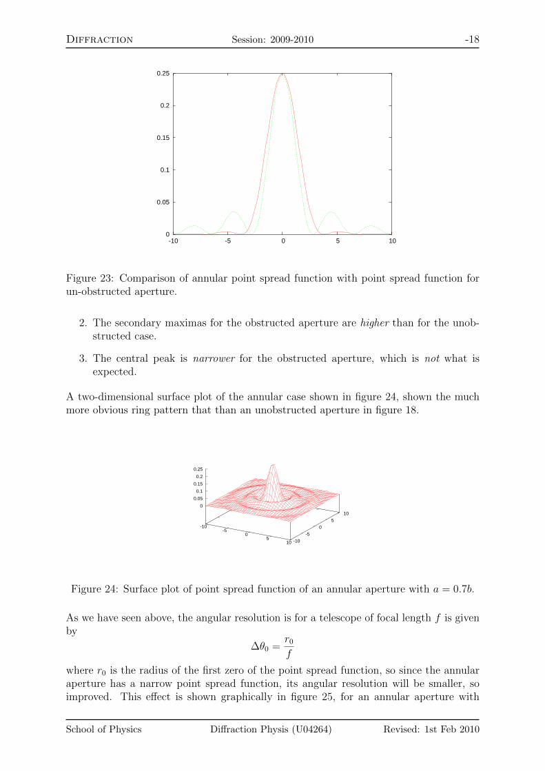
The significance of this complicated expression only becomes apparent when it is plottedand compared to the intensity from an un-obstructed aperture of the same outer diameteras in figure 23, which is plotted for a = 0.7b.

The important feature are:

1. Both have the basic shape with a large central peak and a series of secondarymaximas.



0

0.05

0.1

0.15

0.2

0.25

-10 -5 0 5 10

Figure 23: Comparison of annular point spread function with point spread function forun-obstructed aperture.

2. The secondary maximas for the obstructed aperture are higher than for the unob-structed case.

3. The central peak is narrower for the obstructed aperture, which is not what isexpected.

A two-dimensional surface plot of the annular case shown in figure 24, shown the muchmore obvious ring pattern that than an unobstructed aperture in figure 18.

-10-5

0 5

10 -10

-5

0

5

10

0

0.05

0.1

0.15

0.2

0.25

Figure 24: Surface plot of point spread function of an annular aperture with a = 0.7b.

As we have seen above, the angular resolution is for a telescope of focal length f is givenby

∆θ0 =r0f

where r0 is the radius of the first zero of the point spread function, so since the annularaperture has a narrow point spread function, its angular resolution will be smaller, soimproved. This effect is shown graphically in figure 25, for an annular aperture with



a = 0.7b. The intensity distribution at the Rayleigh limit is plotted on the left, showinga very clear dip, so the points are well resolved. The plot on the right shown the starsseparated by

∆θ =λ

d

where they are still resolved. The actual resolution limit for the annular aperture doesnot have a simple analytical expression, but has to be found numerically, see workshopquestion ??.

0

0.2

0.4

0.6

0.8

1

1.2

-10 -5 0 5 10 0

0.2

0.4

0.6

0.8

1

1.2

-10 -5 0 5 10

Figure 25: Plot of intensity distribution or annular aperture with two stars a) at theRayleigh resolution criteria of ∆θ = 1.22λ/d and b) below the Rayleigh criteria at ∆θ =λ/d

This improved resolution does have a cost, that being the absolute peak intensity with isproportional to the open area of the pupil which is clearly reduced bu the presence of acentral stop.

2.9 Resolution in Real Astronomical Telescopes

The above analysis assumes that an distant point source results in plane wavefrontsacross the input aperture of the system, with the resolution of the system limited onlyby diffraction. This is valid for small high quality system, for example microscopes. thehuman eye, small telescopes, and high quality camera systems; see workshop questionsfor numerical details. When we consider large astronomical telescopes, there is anothervery significant effect, that of the atmosphere. The refractive index of a gas dependson it local density, thus for air, it depends on pressure and temperature. Thus pressureand temperature gradients in the atmosphere result in local refractive index, and thusoptical path length variations, as illustrated in figure 26. This is also why start twinkle.As the atmosphere moves, this introduces a time varying phase aberration across theaperture of the telescope with the speed and extent of the variation depending on thelocal atmospheric conditions. This is known as the seeing conditions. In conditions ofgood seeing, the phase aberration can be considered constant for approximately 1/10th ofsecond, and plane over a region, known as the isoplanatic patch.

Under these conditions, each isoplanatic patch acts as an individual telescope, with the



��

��

Plane Wavefrom Star

Atmosphere

Aberrated Wavefront

Isoplanatic Patch

Image

Figure 26: Schematic of a real terrestrial telescope..

long exposure2. image of the star being an intensity summation of the image from eachpatch. The resolution is therefore limited by the size of the isoplanatic and not the overallaperture of the telescope. In areas of good seeing, the isoplanatic patch is 100 → 150mmin diameter, giving an effective angular resolution of

∆θe ≈ 6× 10−6Rad ≈ 1 sec of arc

for λ = 500 nm and d ≈ 100mm. Since the isoplanatic patches are time-varying, andnot circular, then the shape of the point spread function will be time averaged, and willapproximate a Gaussian with it radius, given by the e−2 intensity position, given, for atelescope of focal length f by approximately ∆θe f .

There are a range of schemes to minimise] this effect,

Telescope Location: Locate the telescope in areas of good seeing, typically high on amountain plateau in an area of stable atmospheric conditions, Hawaii, Tenerif, Arizonaare typical examples. The ultimate is the remove the atmosphere, hence the Hubble SpaceTelescope!

Short Exposures: Use exposure times short compared to the movement of the atmo-sphere, and combine after digital processing. Simples scheme is the selected the sharpimages, align and average.

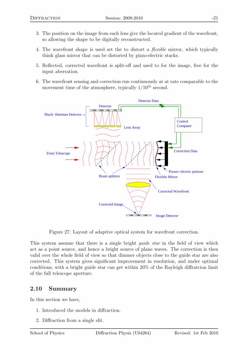
Adaptive Optics: Analyse the inputdistorted wavefront and correct its shape as shown???

in figure 27.

1. Part of the beam is split off and send to a detector.

2. The shape of this distorted wavefront is analysis by a detector system, typicallyconsisting or an array of micro-lenses.

2Long compared with the time constant of the atmosphere



3. The position on the image from each lens give the located gradient of the wavefront,so allowing the shape to be digitally reconstructed.

4. The wavefront shape is used set the to distort a flexible mirror, which typicallythink glass mirror that can be distorted by pizzo-electric stacks.

5. Reflected, corrected wavefront is split-off and used to for the image, free for theinput aberration.

6. The wavefront sensing and correction run continuously at at rate comparable to themovement time of the atmosphere, typically 1/10th second.

��

��

From Telescope

Beam splitters

Detector

Shack−Hartman Detector

Flexible Mirror

Pizzeo−electric pistions

Control Computer

Image Detector

Corrected Wavefront

Corrected Image

Lens Array

Detector Data

Correction Data

Figure 27: Layout of adaptive optical system for wavefront correction.

This system assume that there is a single bright guide star in the field of view whichact as a point source, and hence a bright source of plane waves. The correction is thenvalid over the whole field of view so that dimmer objects close to the guide star are alsocorrected. This system gives significant improvement in resolution, and under optimalconditions, with a bright guide star can get within 20% of the Rayleigh diffratcion limitof the full telescope aperture.

2.10 Summary

In this section we have,

1. Introduced the models in diffraction.

2. Diffraction from a single slit.



3. Diffraction from slit plus lens.

4. The Fourier Approach

5. Diffraction from Two Slits

6. The Diffraction Grating

7. The Grating Spectrometer

8. Practical Diffraction Gratings

9. Diffraction from Circular Aperture

10. Spatial Resolution in Optical Systems

11. The Annular Aperture

12. Resolution in real telescopes.


Topic 2 : Diﬁraction

Documents

Transcript of Topic 2 : Diﬁraction