Top Indian Incomes, 1922-2000 - Thomas...

Top Indian Incomes, 1922-2000

Abhijit Banerjee and Thomas Piketty

This article presents data on the evolution of top incomes and wages for 1922- 2000 in India using individual tax return data. The data show that the shares of the top 0.01 percent, 0.1 percent, and 1 percent in total income shrank substantially from the 1950s to the early to mid-1980s but then rose again, so that today these shares are only slightly below what they were in the 1920s and 1930s. This U-shaped pattern is broadly consistent with the evolution of economic policy in India: From the 1950s to the early to mid-1980s was a period of "socialist" policies in India, whereas the subsequent period, starting with the rise of Rajiv Gandhi, saw a gradual shift toward more probusiness policies. Although the initial share of the top income group was small, the fact that the rich were getting richer had a nontrivial impact on the overall income distribution. Although the impact is not large enough to fully explain the gap observed during the 1990s between average consumption growth shown in National Sample Survey-based data and the national accounts-based data, it is sufficiently large to explain a nonnegligible part of it (20-40 percent).

This article presents data series on top incomes and wages in India during 1922- 2000 based on individual tax return data. It uses tabulations of tax returns published annually by the Indian tax administration to compute the shares of the top 1 percent of the distribution of total income and the top 0.5 percent, 0.1 percent, and 0.01 percent. It does the same for the wage distribution. The analysis does not go below the top 1 percent because incomes below this level are largely exempt from taxation in India.

The series begin in 1922, when the income tax was created in India and thus enables examination of the impact of the Great Depression and World War II on

Abhijit Banerjee is professor of economics in the Department of Economics at the Massachusetts Institute of Technology; his email address is [email protected]. Thomas Piketty is directeur d'études at Ecole des Hautes Etudes en Sciences Sociales, Campus Paris-Jourdan; his email address is [email protected]. The authors are grateful to Tony Atkinson, Amaresh Bagchi, Gaurav Datt, Govinda Rao, Martin Ravallion, T. N. Srinivasan, Suresh Tendulkar, and two anonymous referees for useful discussions; to Sarah Voitchovsky for excellent research assistance; and to the McArthur Foundation for financial support. The complete series is available online in the working paper version of this article (Banerjee and Piketty 2004; www.cepr.org/pubs/new-dps/dp_papers.htm).

THE WORLD BANK ECONOMIC REVIEW, VOL. 19, NO. 1, pp. 1-20 doi:10.1093/wber/lhi001 © The Author 2005. ] Published by Oxford University Press on behalf of the International Bank for Reconstruction and Development / the world bank. All rights reserved. For permissions, please e-mail: [email protected].

1

This content downloaded from 129.199.207.113 on Thu, 29 Oct 2015 15:20:13 UTCAll use subject to JSTOR Terms and Conditions

http://www.jstor.org/page/info/about/policies/terms.jsp

2 THE WORLD BANK ECONOMIC REVIEW, VOL. 19, NO. I

inequality. Of particular interest is the period starting in the 1950s, at the beginning of India's experiment with socialism. This experiment was officially suspended in 1991 with the beginning of the liberalization process, which continued through the 1990s. One explicit goal of the socialist program was to limit the economic power of the elite in the context of a mixed economy. The tax data offer an opportunity to look at the extent to which this program, with its well-known deficiencies, succeeded in its distributional objectives. This is an important part of the assessment of this period, and it offers a window into the broader question of the role of policy in affecting the distribution of income and wealth in a developing economy. With much of the economic activity in these countries outside the formal sector, it is not obvious that there is a lot that policy, especially tax policy, can affect.

Yet the results are consistent with an important role for policy in shaping the distribution of income. In particular, there is evidence of a substantial decline in the share of the elite during the years of socialist planning and a comparable recovery in the postliberalization era. However, the rebound seems to start significantly before the official move toward liberalization.

Given that these results are likely to be controversial, it is worth emphasiz- ing that there are several obvious problems with using tax data, not the least because of tax evasion. These are discussed at some length. Although the results appear to be robust, they are not intended to be definitive but rather to provide a point of departure on an important question about which very little is known, primarily because of data limitations. There are good reasons to suspect that the usual sources of information on income distribution in India - such as consumer expenditure surveys - are not particularly effective at picking up the very rich. This is in part because the rich are such a small share of the population and in part because they are much more likely to refuse to cooperate with the time-consuming process of responding to a consumer expenditure survey.1

Although there is no hard evidence that the rich are indeed being under- counted in India (the Indian consumer expenditure surveys do not, for example, report refusal rates by potential income category), one reason to suspect that this is the case comes from what has been called the Indian growth paradox of the 1990s. According to the standard household expenditure survey conducted by the National Sample Survey (nss), real per capita growth in India during the 1990s was fairly limited. This conclusion stands in sharp contrast with the substantial growth measured by national accounts statistics (nas) over the same period. This puzzle has attracted considerable

1. See, for example, Szekely and Hilgert (1999), who look at a large number of Latin American household surveys and find that the 1 0 highest incomes reported in surveys are often not much larger than the salary of an average manager in the given country at the time of survey. For a systematic comparison of survey and national accounts aggregates in developing countries, see Ravallion (2001).



Banerjee and Piketty 3

attention in recent years,2 and it has been widely suggested that it might simply be that a large part of the growth went to the very rich. However there has been no attempt to directly quantify this possibility.3 The tax data permit taking a useful step in this direction by putting bounds on the extent to which the growth gap can be explained simply as undercounting of the very rich. The analysis here concludes that it can explain between 20 percent and 40 percent of the puzzle. Although this is not negligible, it leaves the bulk of the puzzle unaccounted for, largely because the share of the rich in total income is still relatively small. This suggests that there probably is some deeper problem with the way either the nss or the National Statistical Office (which generates the nas) collects its data.4

The next two sections briefly outline the data and methodology (section I) and present the long-run results (section II). Section III discusses the potential problems with this evidence, and section IV uses the evidence to shed some light on the Indian growth paradox of the 1990s. Section V concludes.

I. Data and Methodology

The tabulations of tax returns published each year by the Indian tax administration in the All-India Income-Tax Statistics series constitute the primary data source used in this study. The first year for which income data are available is 1922/23 and the last year is 1999/2000.5

2. See, for example, Datt (1999), Ravallion (2000), World Bank (2000), and Sundaram and Tendulkar (2001). Recently released data from the 1999-2000 nss round has revealed that growth was larger than expected during the 1990s and that poverty rates did decline over this period, contrary to what most observers believed on the basis of pre- 1999-2000 nss rounds (Deaton and Dreze 2002; Deaton 2003a, b). However, the overall growth gap between nss data and nas data still appears substantial, even after this correction (see table 2). The existence of this growth discrepancy was already a subject of

inquiry in India during the 1980s (see, for example, Minhas 1988 and Minhas and Kansal 1990), but the

gap observed during the 1990s appears to be substantially larger than the gap during previous decades. For a broader, international perspective on the survey and national accounts debate, see Deaton (2003c).

3. Sundaram and Tendulkar (2001) find that the nss-nas gap is particularly important for commod- ities that are more heavily consumed by higher income groups, thereby providing indirect evidence for the

explanation based on rising inequality. 4. See Bhalla (2002) tor a negative view or the nss approach, ror more balanced discussions or the

relative merits of survey and national accounts aggregates in developing economies, see Ravallion (2001) and Deaton (2003c).

5. References to the relevant All-India Income-Tax Statistics (aiits) publications are given in the working paper version of this study (Banerjee and Piketty 2004, table A0). Financial years run from April 1 to March 31 in India, so that 1922/23 refers to the period running from April 1, 1922, to March 31, 1923, for example, ahts

publications refer to assessment years (the year in which the income is assessed), whereas this study refer to income years, or the year in which the income was earned. Thus, for example, aiits 1 923/24 contains the data on income year 1922/23. aiits 2000/01 data (income year 1999/2000) were not yet available when the study was

updated, so the income year 1 999/2000 data for top incomes were obtained by inflating the 1 998/99 data by the nominal 1999-2000/1998-99 per tax unit national income growth rate. This approximation probably leads to an underestimate of top income growth, but as there was no large nss round for 1998/99, it was easier to make

comparison with 1999/2000 as the end point.




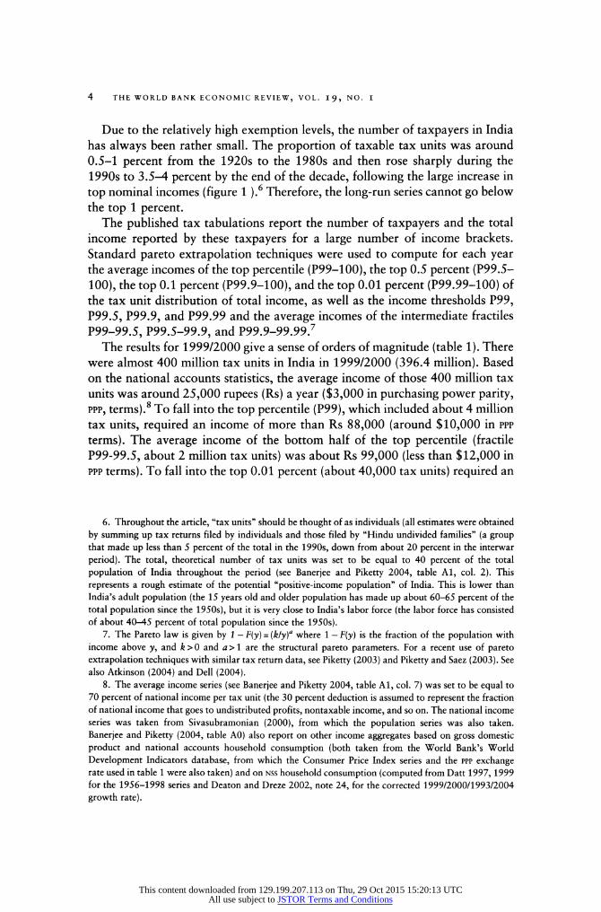
Due to the relatively high exemption levels, the number of taxpayers in India has always been rather small. The proportion of taxable tax units was around 0.5-1 percent from the 1920s to the 1980s and then rose sharply during the 1990s to 3.5-4 percent by the end of the decade, following the large increase in top nominal incomes (figure 1 ).6 Therefore, the long-run series cannot go below the top 1 percent.

The published tax tabulations report the number of taxpayers and the total income reported by these taxpayers for a large number of income brackets. Standard pareto extrapolation techniques were used to compute for each year the average incomes of the top percentile (P99-100), the top 0.5 percent (P99.5- 100), the top 0.1 percent (P99.9-100), and the top 0.01 percent (P99.99-100) of the tax unit distribution of total income, as well as the income thresholds P99, P99.5, P99.9, and P99.99 and the average incomes of the intermediate fractiles P99-99.5, P99.5-99.9, and P99.9-99.99.7

The results for 1999/2000 give a sense of orders of magnitude (table 1). There were almost 400 million tax units in India in 1999/2000 (396.4 million). Based on the national accounts statistics, the average income of those 400 million tax units was around 25,000 rupees (Rs) a year ($3,000 in purchasing power parity, ppp, terms).8 To fall into the top percentile (P99), which included about 4 million tax units, required an income of more than Rs 88,000 (around $10,000 in ppp terms). The average income of the bottom half of the top percentile (fractile P99-99.5, about 2 million tax units) was about Rs 99,000 (less than $12,000 in ppp terms). To fall into the top 0.01 percent (about 40,000 tax units) required an

6. Throughout the article, "tax units" should be thought of as individuals (all estimates were obtained by summing up tax returns filed by individuals and those filed by "Hindu undivided families" (a group that made up less than 5 percent of the total in the 1990s, down from about 20 percent in the interwar period). The total, theoretical number of tax units was set to be equal to 40 percent of the total population of India throughout the period (see Banerjee and Piketty 2004, table Al, col. 2). This represents a rough estimate of the potential "positive-income population" of India. This is lower than India's adult population (the 15 years old and older population has made up about 60-65 percent of the total population since the 1950s), but it is very close to India's labor force (the labor force has consisted of about 40-45 percent of total population since the 1950s).

7. The Pareto law is given by 1 - F{y) = {k/y)a where 1 - F{y) is the fraction of the population with income above y, and k > 0 and a > 1 are the structural pareto parameters. For a recent use of pareto extrapolation techniques with similar tax return data, see Piketty (2003) and Piketty and Saez (2003). See also Atkinson (2004) and Dell (2004).

8. The average income series (see Banerjee and Piketty 2004, table Al, col. 7) was set to be equal to 70 percent of national income per tax unit (the 30 percent deduction is assumed to represent the fraction of national income that goes to undistributed profits, nontaxable income, and so on. The national income series was taken from Sivasubramonian (2000), from which the population series was also taken. Banerjee and Piketty (2004, table A0) also report on other income aggregates based on gross domestic product and national accounts household consumption (both taken from the World Bank's World Development Indicators database, from which the Consumer Price Index series and the ppp exchange rate used in table 1 were also taken) and on nss household consumption (computed from Datt 1997, 1999 for the 1956-1998 series and Deaton and Dreze 2002, note 24, for the corrected 1999/2000/1993/2004 growth rate).




Figure 1. Proportion of Taxable Tax Units in India, 1922-2000 (percent)

Source: Authors' computations using tax return data; see Banerjee and Piketty (2004, table Al).

income of more than Rs 1.4 million ($160,000 in ppp terms), and the average income above that threshold was more than Rs 4 million ($470,000 in ppp terms).9

As is the case in other countries, the top of the income distribution in India appears to be very precisely approximated by the pareto structural form.10 However, the estimates for the recent period are subject to sampling error: The official tax tabulations were based on the entire population until the early 1990s (as is the case in most Organisation for Economic Co-operation and Development countries),11 but they now seem to be based on uniform samples of all tax returns. Although there is uncertainty about the new sampling

9. To put these numbers in global perspective, consider that India's 1999/2000 P99.99 threshold (about $160,000 in ppp terms) is located midway between U.S. 1998 thresholds for P95 ($107,000) and P99 ($230,000); see Piketty and Saez (2003, table 1). India's 1999/2000 P99.9 threshold (about 34,000$ in ppp terms) is well below the U.S. 1998 P90 threshold ($82,000).

10. In the same way as for other countries (see previous references), the extrapolation results were checked and were found to be virtually unaffected by the choice of extrapolation thresholds used to estimate the structural parameters. Pareto coefficients are locally very stable in India, as they are in other countries. Before the 1990s, less than 1 percent of individuals were subject to tax, and the lowest threshold available was used to estimate the top percentile threshold, P99 (given that pareto coefficients are in practice very stable, the resulting estimates appear to be as precise as estimates for thresholds P99.5 and higher).

11. Or they were based on stratified samples with sampling rates close to 100 percent for top incomes.



*4\2 £ «§ 2 ^ 00 N ON 't (N S O W> ̂f, U ^ ^ ^0 <N K V£> ON O

g « g § ^ ^t,0^^ S

2 o2 m "-> ̂ ©^ r^ vo g

<^£| ^ . ̂ S * 5 <=>

la ,^ O M O\ CO O\ 2 II Rum «> N + (S »00 •« -rirt «> g « vo oo on, ■* <s^ •« -rirt 5;

1 1 v*h OOOOO ^^ "

.^ o^ ©^ vo^ r^ vo^ S >< « J5 o rî 10 vrT oC o ^ J3 h» O OO 00 >O ro (N ^ 5 gx ^- O\ io rn ^^-i4

s 8 ■S3

O cjn rt Œs "H lO ON CJ\ -. ax ON

^ -S ON* ON* O< 8 -.

12 ax

g ô^ôôi, I |g =! ^ onon on T;^^

^ J3 g 3 Sod

On u c^- ■

hJ^G^ ^^^^ G?§

►- « «3 m ̂ fl S G00

g S "5 ë ^ n ^ °\ g g h y^S OOrfONOO ^Î3^^

S II S ONONONON^^d

-n «^ 8$ I | § < S S ONONONON^^d H <

Se ££S£ 8

6




procedure, the sampling rate seems to be sufficiently large to guarantee that the estimated trends for top income shares are statistically significant.12

Official tax publications also include tabulations of the amounts of income in each category (wages, business income, dividends, interest, and so on) for each income bracket. In particular, there are separate tables for wage earners, by far the largest subgroup. This enabled separating estimates for top wage fractiles, which could then be compared with the estimates for top fractiles of total income (see later discussion).13

II. The Long-Run Dynamics of Top Income Shares, 1922-2000

The results show that income inequality (as measured by the income shares of those in the top income groups) follows a U-shaped pattern over 1922-2000 (figure 2 ). The top 0.01 percent income share fluctuates around 2-2.5 percent of total income from the 1920s to the 1950s. It then gradually falls from about 1.5-2 percent of total income in the 1950s to less than 0.5 percent in the early 1980s. It rises again during the 1980s and 1990s and reaches 1.5-2 percent again during the late 1990s. This means that the average income of the top 0.01 percent of the income distribution was about 150-200 times larger than the average income of the entire population during the 1950s. The difference fell to less than 50 times larger than the average income in the early 1980s, but then rose again to 150-200 times larger during the late 1990s.

The exact turning point is also of some interest. The decline in the share of the top 0.01 percent is relatively rapid until 1974/75 (see figure 3). Then it slows considerably, but there is still a clear downward trend until 1980/81. Then the trend reverses, moving upward throughout the 1980s, reaching a peak in 1988/89. During the 1980s the share of the top 0.01 percent more than doubles - from less than 0.4 percent to more than 0.8 percent. But it then reverses again, and by 1991/92 the share is back below 0.6 percent. Then it takes off, and after 1995/96 it remains in the 1.5-2 percent range.

12. According to the tax administration statistics division, the sampling rate is about 1 percent and approximately uniform (the official tax publications do not include any precise information about sampling design and rate). Given India's large population, this implies that the estimate for the top 1 percent income share (8.95 percent of total income in 1999/2000; see Banerjee and Piketty 2004, table A4) has a standard error of about 0.04 percent and that the estimate for the top 0.01 percent income share (1.57 percent of total income in 1999/2000; see Banerjee and Piketty 2004, table A4) has a standard error of about 0.08 percent. There is some evidence, however, that the sampling design is changing and that published tabulations were becoming more volatile by the end of the period. In particular, the tabulations for income year 1997/98 (assessed year 1998/99) contain far too many individual taxpayers above 1 million rupees, suggesting that something went wrong in the sampling design that year. The 1997/98 estimates were corrected downward on the basis of 1996/97 and 1998/99 tabulations.

13. Published wage tabulations for income year 1996/97 and 1997/98 appear to suffer from sampling design failures (top wages are clearly truncated in 1996/97, and they are too numerous in 1997/98). The estimates for those two years were corrected on the basis of 1995/96 and 1998/99 data.




Figure 2. The Top 0.01 Percent Income Share in India, 1922-2000 (percent)

Source: Authors' computations using tax return data; see Banerjee and Piketty (2004, table A4).

Figure 3. The Top 0.1 Percent Income Share in India, 1922-2000 (percent)





A similar (though less pronounced) U-shaped pattern is also observed for the top 1 percent income share, which went from about 12-13 percent during the 1950s to 4-5 percent in the early 1980s and to 9-10 percent in the late 1990s (figure 4). Once again the turning point seems to be around 1980/81, and during the 1980s the share of the top 1 percent also doubles. Then, as with the share of the top 0.01 percent, there is a period of retrenchment that lasts till 1991/92, followed by a renewed upward movement.

A comparison of these trends reveals another intriguing fact: Although in the 1980s the share of the top 1 percent increases almost as quickly as the share of the top 0.01 percent (see figures 2 and 4), in the 1990s there is a clear divergence between what is happening in the top 0.01 percent and in the rest of the top 1 percent. To confirm that this is the case, the top percentile is broken into four fractiles: P99-99.5, P99.5-99.9, P99.9-99.99, and P99.99-100. During the 1987-2000 period, only those in the top 0.1 percent enjoyed income growth rates faster than the growth rate of gdp per capita (table 2). This contrasts with what is observed when the period includes the 1980s, which shows evidence of above average growth for the entire top percentile (table 3).

Although 1980/81 is clearly the year when the data series turn around, it is not possible to date the true turnaround with as much precision, because the income share of the rich is also affected by short-run, cyclical factors. It may be that the data series puts the turnaround in 1980/81 only because no allowance was made for the deep recession of 1979/80 and 1980/81, which hurt the rich. Thus what

Figure 4. The Top 1 Percent Income Share in India, 1922-2000 (percent)





Table 2. Top Income Growth during the 1990s: 1999/2000 versus 1987/88 (percent) Item Nominal Growth Real Growth

Household consumption per capita (nss) +242 +19 gdp per capita (nas) +337 +52 Household consumption per capita (nas) +304 +40 National income per tax unit (nas) +346 +55 Top income fractiles (tax returns) P99-100 +392 +71 P99.5-100 +412 +78 P99.9-100 +548 +125 P99.99-100 +1,009 +285 P99-99.5 +331 +50 P99.5-99.9 +317 +45 P99.9-99.99 +393 +71 P99.99-100 +1,009 +285 Consumer price index +188 Share of growth gap accounted for by P99-100 20.1 P99.5-100 17.2 P99.9-100 12.7 P99.99-100 8.0

Source: Authors' computations using tax return, nas, and nss data; see Banerjee and Piketty (2004, tables A1-A3).

Table 3. Top Income Growth in India during the 1980s-1990s: 1999/2000 versus 1981/82 (percent) Item Nominal Growth Real Growth

Household consumption per capita (nss) +487 +25 gdp per capita (nas) +700 +70 Household consumption per capita (nas) +599 +49 National income per tax unit (nas) +688 +68 Top income fractiles (tax return) P99-100 +1,508 +242 P99.5-100 +1,747 +293 P99.9-100 +2,270 +404 P99.99-100 +3,980 +767 P99-99.5 +992 +132 P99.5-99.9 +1,392 +217 P99.9-99.99 +1,698 +282 P99.99-100 +3,980 +767 cpi +370 Share of growth gap accounted for by P99-100 39.7 P99.5-100 33.5 P99.9-100 19.1 P99.99-100 9.3

Source: Authors' computations using tax return, nas, and nss data; see Banerjee and Piketty (2004, tables A1-A3).



Barter jee and Piketty 11

appears as a sharp upward trend starting in 1981 may be just a reversion in 1981/ 82 and 1982783 to the preexisting trend. Therefore, rather than ascribing the turnaround to a single year, it is ascribed to the early to mid-1980s.

The fact that the turnaround is so early makes it hard to attribute it to the formal process of liberalization. Indeed, given the nature of the data, it cannot be entirely ruled out that the driving factor was either a shift in the global economic environ- ment or a part of the natural evolution of a mixed economy. However, the timing of the turnaround is also consistent with the view that there was a structural shift in the Indian economy in the early to mid 1980s. Delong (2001) and Rodrik and Subramanian (2004), based on macro time-series data, date the acceleration in the growth rate of the Indian economy to the early to mid-1980s, rather than the early 1990s. They suggest that this may have to do with a shift of power within the ruling Congress Party toward a more technocratic, probusiness group associated with Rajiv Gandhi, who entered politics in 1981 following his brother's death and became prime minister in 1984. Available macro series also show that the wage share in the private corporate sector has been declining in India since the early to mid-1980s (in contrast to the 1970s, when the profit share was declining; see Nagaraj 2000, figure 7, and Tendulkar 2003, table 14), which is again consistent with the time for the turnaround proposed here.

Also, although the turnaround was earlier, the data suggest a definite acceleration in the growth of the share of the top 0.01 percent after 1991. Moreover, this contrasts with what is observed for the top 1 percent, suggesting that what happened after 1991 was qualitatively different from what happened before, and even more biased in favor of the ultra-rich.

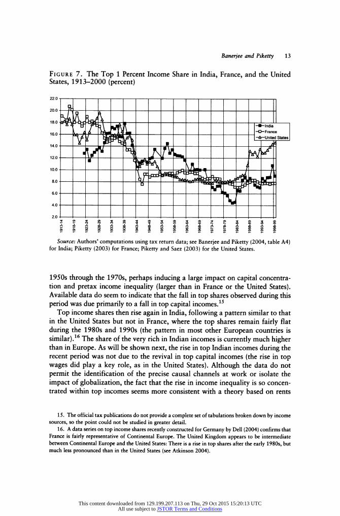
Finally, there is tentative evidence suggesting that what happened in India over the entire period was not simply a reflection of forces that were affecting countries all over the world. A comparison of India with France and the United States during the 1950s and 1960s shows that India was less egalitarian than the other two countries (figures 5 -7). The top 0.01 percent earned a substantially higher share of total income in India. Subsequently, however, top income shares declined con- tinuously in India during the 1960s and the 1970s and fell below the levels in France and the United States during the early 1980s. That the decline in India occurred mostly during the 1950s to 1970s (rather than during the interwar and World War II period) seems consistent with the interpretation posited by Piketty (2003) and Piketty and Saez (2003) to explain the French and U.S. trajectories: The shocks induced by the Great Depression of the 1930s and World War II were less severe in India,14 whereas tax progressivity was extremely high in India during the

14. Note that unlike in France, the United States, or the United Kingdom, top income shares in India were actually rising during the Great Depression of the 1930s. Top Indian nominal incomes did decline

during the 1930s, but less rapidly than the national income and wage series computed by Sivasubramonian (2000). This probably reflects the fact that India had a very different position than France, the United States, or the United Kingdom in the world division of labor during the 1930s (Indian entrepreneurs might have benefited from the drop in world manufacturing output and raw material prices).




FigureS. The Top 0.01 Percent Income Share in India, France, and the United States, 1913-2000 (percent)

Figure 6. The Top 0.1 Percent Income Share in India, France, the United States, and the United Kingdom, 1913-2000 (percent)




Figure 7. The Top 1 Percent Income Share in India, France, and the United States, 1913-2000 (percent)

1950s through the 1970s, perhaps inducing a large impact on capital concentra- tion and pretax income inequality (larger than in France or the United States). Available data do seem to indicate that the fall in top shares observed during this period was due primarily to a fall in top capital incomes.15

Top income shares then rise again in India, following a pattern similar to that in the United States but not in France, where the top shares remain fairly flat during the 1980s and 1990s (the pattern in most other European countries is similar).16 The share of the very rich in Indian incomes is currently much higher than in Europe. As will be shown next, the rise in top Indian incomes during the recent period was not due to the revival in top capital incomes (the rise in top wages did play a key role, as in the United States). Although the data do not permit the identification of the precise causal channels at work or isolate the impact of globalization, the fact that the rise in income inequality is so concen- trated within top incomes seems more consistent with a theory based on rents

15. The official tax publications do not provide a complete set of tabulations broken down by income sources, so the point could not be studied in greater detail.

16. A data series on top income shares recently constructed for Germany by Dell (2004) confirms that France is fairly representative of Continental Europe. The United Kingdom appears to be intermediate between Continental Europe and the United States: There is a rise in top shares after the early 1980s, but much less pronounced than in the United States (see Atkinson 2004).




and market frictions (see, for example, Banerjee and Newman 2003) than with a theory based solely on skills and technological complementarity (in which the rise in inequality in developing countries reflects a low-skilled labor force unable to benefit from globalization; see, for example, Kremer and Maskin 2003).

III. Measurement Issues

The presumption so far has been that what has been measured is the actual income share of the rich. There are a number of reasons why this may not be true. First, despite extensive efforts, it was not possible to determine exactly what changes were made during the 1990s in the procedure for generating the samples used to create the tax tables. From informal conversations with Indian tax officials, it seems that at least in recent years the procedure is more an informal attempt to sample randomly than a precise random sample. To the extent that this increases the risk of the data being clustered, the implication is that the within-sample variance might overstate the precision of the data. This remains a possibility, but for the most part the trends seem quite stable. Although the results for single years or sets of years may reflect sampling variation, the fact that in every year between 1973/74 and 1992/93 the share of the top 0.01 percent is less than 0.85 percent (and in every year but two it is less than 0.7 percent) and that in 1995/96 and every year after that it is greater than 1.5 percent makes the results appear much more robust. The two intervening years, 1993/94 and 1994/95 show, as might be hoped, shares between 0.7 percent and 1.5 percent for the top 0.01 percent.

A more serious problem is that the surge in top incomes may reflect improve- ments in the income tax department's ability to measure (and hence tax) the incomes of the wealthy. The tax cuts in the early 1990s might have reduced the incentives among the wealthy for evading taxes. Note, however, that the overall decline in the top marginal rate, though nonmonotonic, was quite moderate: The top marginal tax rate dropped from 50 percent in 1987/88 to 40 percent in 1999/2000 (figure 8). By comparison, the change in the share of the top 0.01 percent was huge: It went up from 0.7 percent in 1987/88 to more than 1.5 percent in 1999/2000. If this entire change is to be explained by a shift in tax rates, the implied elasticity would have to be enormous.

Experience elsewhere also suggests that the rise of top incomes can be explained by nontax structural factors (changing social norms, booming economy, international trade, and globalization) rather than by tax changes and increased incentives to report top incomes. The consensus in the United States seems to be that while short-run elasticities can be substantial,17 the medium- and long-run elasticity of top taxable incomes with respect to top tax rates is

17. Reflecting mostly income relabeling or changes in timing of the exercise of bonuses or stock options.




Figure 8. The Top 0.01 Percent Income Share and the Top Marginal Income Tax Rate in India, 1981-2000 (percent)

Table 4. Top Wage Growth in India during the 1990s: 1999/2000 versus 1987/88 (percent) Item Nominal growth Real growth

Household consumption per capita (nss) +242 +19 gdp per capita (nas) +337 +52 Household consumption per capita (nas) +304 +40 National income per tax unit (nas) +346 +55 Top wage fractiles (tax returns) tP99-100 +420 +81 P99.5-100 +492 +105 P99.9-100 +551 +126 P99.99-100 +955 +266 P99-99.5 +246 +20 P99.5-99.9 +470 +98 P99.9-99.99 +448 +94 P99.99-100 +955 +266 cpi 188

Source: Authors' computations using tax return, nas, and nss data; see Banerjee and Piketty (2004, tables Al, A5, and A6).




probably modest. The rise in top income shares in the United States during 1970-2000 seems to reflect real economic change (rather than pure fiscal manipulation): The top shares started rising well before Tax Reform Act of 1986, and the rise continued at an even faster pace during the 1990s, despite the 1993 rise in top tax rates (Goolsbee 2000; Piketty and Saez 2003). In China top income shares rose substantially during 1986-2001 (twice as fast as in India), despite the fact that top Chinese income tax rates have remained unchanged since the early 1980s (Piketty and Qian 2004).

Of course, the effect of tax changes in India could have been reinforced by spectacular improvement in the collection technology (as well as increased incentives on the taxpayer side). There were a number of innovations in tax collection in the 1990s, such as the 1998 introduction of the "one in six rule" that required everyone who satisfied at least one of six criteria (such as owning a car and travel abroad) to file a tax return.

To further investigate this issue, the exercise was rerun for wages only. Wages are much less subject to tax evasion than are nonwage income, because taxes are typically deducted at the source and employers have a strong incentive to report what they pay because wage payments are deductible from employers' taxes. Therefore, if better collection made the difference, wage incomes would be expected to have grown much more slowly than other income. The results show that top wages (table 4) increased essentially in step with top incomes (see table 2) during the 1990s, rising 81 percent between 1987/88 and 1999/ 2000 for the top percentile of the wage distribution compared with 71 percent for the top percentile of the income distribution. This is consistent with the fact that wages as a share of the total income of the top percentile increased somewhat during this period (from 28 percent to 31 percent).

The interpretation that there was a "real" increase in top incomes (especially top wages) in India during the 1990s is also consistent with the evolution of the public sector salary scale. Following a succession of Pay Commissions, including the well-known Fifth Pay Commission, whose recommendations were imple- mented in 1997, the salaries of central government employees were raised sharply in India during the 1990s (see, for example, Kochar 2003). According to computations for this study (based on published public sector salary scales), the Fifth Pay Commission alone can account for a substantial part of the rise in the number of top income taxpayers in India between 1994 and 1997. Central government employees made up about 7 percent of all income tax taxpayers in India in 1994 (fewer than 500,000 central government taxpayers, of total of about 7 million taxpayers), and following the pay rise they made up almost 30 percent of all taxpayers by 1997 (about 3.2 million central government taxpayers, of a total of 11 million). According to these computations, of the 4 million extra taxpayers recorded between 1994 and 1997, around 2.7 million (almost 70 percent) were central government employees. The very top wage of the central government salary scale was 98,000 Rs (9,000 Rs a month) in 1994 (which was just a little bit above the P99.5 threshold), and it was raised to




360,000 Rs (30,000 Rs a month) in 1997 (which was well above the P99.9 threshold).18 However, it does not seem to be the case that public sector wage increases were the primary driver behind the increase in inequality in the 1990s. Most of the rise in top Indian income shares actually took place before 1997, and it is likely that the revised scale put forward by the Fifth Commission was itself a response to the large rise in top private sector wages that had taken place in previous years.19

IV. The Growth Paradox of the 1990s

Can the fact that the rich were getting richer help solve what has been called the Indian growth paradox of the 1990s? Table 2 illustrates this paradox: For the period 1987-2000, it compares the growth rate of average consumption as reported in the nss, with the growth rate of average income and consumption from the nas, as well as the top incomes from the tax returns. The years 1987/88 and 1999/2000 were chosen because there were large rounds of the nss surveys in those years, enabling more precise estimates of the nss-nas gap.20 To elim- inate the effect of using different deflators, nominal growth performance was compared first and then real growth performance was computed using the same deflator for all the series (the Consumer Price Index, cpi).

18. All these computations on public sector wages were made using the 1994 and 1997 (post-Fifth Commission) central government salary scales published in the "Report of the 5th Central Pay Commis- sion" ("Distribution of Filled Posts in Central Government and Union Territories in Different Scales of Pay, as on 31.3.1994," Government of India Press, New Delhi, 1997) and in the Gazette of India (Special Issue, The First Schedule - Part A, "Revised scales for posts carrying present scales in Group A, B, C and D," Government of India Press, New Delhi, 1997). In 1994, the central government scale ranked from scale 1 (9,000 Rs a month) to scale 62 (750 Rs a month), and all employees in scales 1 to 46 (approximately 500,000 employees) were subject to tax (that is, they had annual incomes greater than 28,000 Rs, which was the base exemption level in 1994, excluding all special deductions). In 1997 the (revised) scale ranked from scale S-34 (30,000 Rs a month, previously scale 1) to scale S-l (2,550 Rs a month, previously scale 62), and all employees in (revised) scales S-34 to S-3 (approximately 3.2 million people) were subject to tax (that is, they had annual incomes of more than 40,000 Rs, which was the base exemption level in 1997, excluding all special deductions). Note that these numbers include only central government employees strictly speaking and that they would need to be scaled up substantially to take other government employees into account. In 1994 there were about 4 million central government employees, and the total number of workers employed by state governments, quasi-government bodies, and local bodies was about 3.5 times as large. In principle the Fifth Pay Commission revised scales also applied to these noncentral government employees, but salary distribution for these employees could not be found (such a document apparently exists only for the central government).

19. Such a view would be consistent with the fact the ceiling on private sector executive compensation was repealed as early as 1991.

20. Intermediate nss surveys were conducted between the two large surveys of 1987/88 and 1993/94 and between the two large surveys of 1993/94 and 1999/2000, but these were based on smaller samples and are considered less reliable. The 1999/2000 per capita consumption estimates come from Deaton and Dreze (2002), who corrected the data for changes in the recall period (all surveys until 1993/94 were conducted with a 30-day recall period, but the nss has experimented with a 7-day recall period since then).




According to the nss data, real growth was fairly limited in India during the 1990s: Per capita consumption increased by only 19 percent in real terms between 1987/88 and 1999/2000. According to nas data, however, real growth was more than twice as large: Both per capita gdp and national income increased by more than 50 percent in real terms, and per capita household consumption increased by 40 percent. This nss-nas gap is referred to as the Indian growth paradox and has been the subject of much discussion in recent years.21

Table 2 raises the possibility that the very large growth of top incomes during the 1990s might help solve this puzzle. The average income growth among the top 1 percent of the tax units was 71 percent in real terms between 1987/88 and 1999/2000, which is substantially more than average growth according to the national accounts. Moreover, the higher up in the top 1 percent, the higher the growth (up to 285 percent for the top 0.01 percent).

What fraction of the nss-nas gap can be explained by the huge growth performance of very top incomes? Assume that the nss is unable to record any of the extra growth enjoyed by the top 1 percent (say, the people in the top 1 percent do not report their extra growth to the nss or do not report anything at all). By the calculations reported here, the top 1 percent share in total consumption was around 8 percent in 1987/88.22 Since the average income of the top 1 percent increased by 71 percent in real terms between 1987/88 and 1999/2000 according to the tax returns, compared with 19 percent for average nss consumption, this implies that nss growth was 3.55 percent less than it would have been without the misreporting (0.0812 x [1.71/1.19- 1] = 3.55). This implies that the growing incomes among the top 1 percent can explain at most 20.1 percent (3.55/[1.40/1.19 - 1] = 20.1) of the nss-nas gap (see table 2).23 This is significant, but it still leaves 80 percent of the puzzle unexplained. The problem lies in the fact that almost all the extraordinary growth was among the top 0.1 percent, and the weight of this group is simply not large enough to have an impact on aggregate statistics of the necessary magnitude. For the rise of inequality to fully explain the nss-nas gap, there would have to have been very high income growth at the bottom of the top 1 percent and not simply among those in the top 0.1 percent.

Top income growth can explain a larger proportion of the nss-nas gap if the analysis starts in the 1980s. For instance, under the same assumptions, the top 1 percent can explain almost 40 percent of the cumulative nss-nas gap over the

21. See previous references. Real growth during the 1990s would be somewhat higher if the gdp deflator were used instead of the cpi, but the nss-nas gap would obviously not change.

22. According to estimates for this study (computed with 70 percent of national income as the income denominator), the top percentile income share was 8.12 percent in 1987/88 (see Banerjee and Piketty 2004, table A3).

23. This is in a sense a lower bound, because the 1987/88 top percentile share is being used as the baseline for this computation, and the share was higher for later years.



Barter jee and Fiketty 19

1981-2000 period (table 3). This is because the bottom of the top percentile enjoyed rapid income growth in the 1980s (see figures 2-4). The booming Indian elite of the 1980s and 1990s seems too thin to explain all of the growth puzzle, but large enough to account for a nonnegligible part of it.

V. Conclusion

The results suggest that the gradual liberalization of the Indian economy did make it possible for the rich (the top 1 percent) to substantially increase their share of total income. However, although in the 1980s the gains were shared by everyone in the top 1 percent, in the 1990s the big gains went only to those in the top 0.1 percent. The 1990s were also the period when the economy was opened. This suggests the possibility that the ultra-rich were able to corner most of the income gains in the 1990s because they alone were in a position to sell what world markets wanted.24 It would be interesting to see whether in the coming years, as more people position themselves to benefit from world markets, the share of the rich and the ultra-rich stops growing and even begins to shrink. To be able to determine this and to shed light on related issues, more research (and better data) are needed that focus on the rich.

24. The point is that one does not have to be rich on a global scale to be counted among the rich in India and even among the ultra-rich (see table 1). Even those who are paid about as much as an average American make it into the group of the ultra-rich.

References

Atkinson, Anthony B. 2004. "Top Incomes in the United Kingdom over the Twentieth Century." Nuffield College, Oxford.

Banerjee, Abhijit, and Andrew Newman. 2003. "Inequality, Growth and Trade Policy." Massachusetts Institute of Technology, Cambridge, Mass, and London School of Ecocomics and Political Science.

Banerjee, Abhijit, and Thomas Piketty. 2004. "Top Indian Incomes, 1922-2000." cepr Discussion Paper 4632. Centre for Economic Policy Research, London.

Bhalla, Surjit S. 2002. Imagine There Is No Country: Poverty, Inequality and Growth in the Era of Globalization. Washington, D.C.: Institute for International Economics.

Datt, Gaurav. 1997. "Poverty in India 1951-1994: Trends and Decompositions." World Bank, Washington, D.C.

. 1999. "Has Poverty Declined since Economic Reforms?" Economic and Political Weekly, December 11-17.

Deaton, Angus. 2003a. "Adjusted Indian Poverty Estimates for 1999-2000." Economic and Political

Weekly, January 25. . 2003b. "How to Monitor Poverty for the Millennium Development Goals." Journal of Human

Development 4(3):353-78. . 2003c. Measuring Poverty in a Growing World (or Measuring Growth in a Poor World), nber

Working Paper 9822, Cambridge, Mass.




Deaton, Angus, and Jean Dreze. 2002. "Poverty and Inequality in India - A Re-Examination." Economic and Political Weekly. September 7.

Dell, Fabien. 2004. "Top Incomes in Germany, 1880-2000." Campus Paris-Jourdan, Paris.

Delong, J. Bradford. 2001. "India Since Independence: An Analytical Growth Narrative." University of California, Berkeley.

Goolsbee, A. 2000. "What Happens When You Tax the Rich? Evidence from Executive Compensation." Journal of Political Economy 108(2):352-78.

Kochar, Anjini. 2003. "Government, Schooling and Poverty: The Trickle-Down Benefits of Higher Schooling in India." Stanford University, Center for Research on Economic Development and Policy Reform, Palo Alto, Calif.

Kremer, Michael, and Eric Maskin. 2003. "Globalization and Inequality." Harvard University, Cam- bridge, Mass.

Minhas, B. S. 1988. "Validation of Large Scale Sample Survey Data: Case of nss Estimates of Household Consumption Expenditure." Sankhya, Series B, 50(3), Suppl.

Minhas, B. S., and S. M. Kansal. 1990. "Firmness, Fluidity and Margins of Uncertainty in the National Accounts Estimates of PCE in the 1980s." Journal of Income and Wealth 12(1).

Nagaraj, R. 2000. "Indian Economy since 1980? Virtuous Growth or Polarization?" Economic and Political Weekly, August 5.

Piketty, Thomas. 2003. "Income Inequality in France, 1901-1998." Journal of Political Economy lll(5):1004-42.

Piketty, Thomas, and Nancy Qian. 2004. "Income Inequality and Progressive Income Taxation in China and India, 1986-2010." Campus Paris-Jourdan, Paris, and Massachusetts Institute of Technology, Cambridge, Mass.

Piketty, Thomas, and Emmanuel Saez. 2003. "Income Inequality in the United States, 1913-1998." Quarterly Journal of Economics 118(l):l-39.

Ravallion, Martin. 2000. "Should Poverty Measures Be Anchored to the National Accounts?" Economic and Political Weekly, August 26-September 2.

. 2001. "Measuring Aggregate Welfare in Developing Countries: How Well Do National Accounts and Surveys Agree?" World Bank, Washington, D.C.

Rodrik, Dani, and Arvind Subramanian. 2004. The Mystery of the Indian Growth Transition, nber Working Paper 10376, Cambridge, Mass.

Sivasubramonian, S. 2000. The National Income of India in the Twentieth Century. Delhi: Oxford University Press.

Sundaram, K., and Suresh D. Tendulkar. 2001. "nas-nss Estimates of Private Consumption for Poverty Estimation." Economic and Political Weekly, January 13-20.

Szekely, Miguel, and Marianne Hilgert. 1999. "What's Behind the Inequality We Measure: An Investiga- tion Using Latin American Data." Inter- American Development Bank, Washington, D.C.

Tendulkar, Suresh D. 2003. "Organised Labour Market in India - Pre and Post Reform." University of Delhi, Delhi School of Economics.

World Bank. 2000. India- Policies to Reduce Poverty and Accelerate Sustainable Development. Report 19471-IN. Washington, D.C.



Top Indian Incomes, 1922-2000 - Thomas...

Documents

Transcript of Top Indian Incomes, 1922-2000 - Thomas...