Tariffs, Vertical Specialization and Oligopoly∗

Tomohiro Ara†

Fukushima University

Arghya Ghosh‡

University of New South Wales

September 2015

Abstract

We examine optimal tariffs in an environment with vertical specialization where theHome country specializes in final goods and the Foreign country specializes in intermediateinputs. A matched Home-Foreign pair bargains simultaneously over the input price and thelevel of output, and competes a la Cournot with other matched pairs in markets. We find thatthe optimal Home tariff rate is strictly decreasing in the bargaining power of Home firms,and an increase in the Home firms’ bargaining power might therefore raise Foreign profits.Under an endogenous market structure with entry followed by matching, the relationshipbetween bargaining power and output is non-monotone if the demand function is strictlyconcave or convex. This in turn induces a non-monotone relationship between the optimaltariff and bargaining power for a class of demand functions. For linear demand, free trade isoptimal irrespective of bargaining power. We show that non-monotonicity result is retainedunder endogenous bargaining power.

Keywords: Tariffs, Oligopoly, Bargaining Power, Outsourcing, Free EntryJEL Classification Numbers: F12, F13

∗We thank the editor (Theo Eicher), an associate editor and two anonymous referees for thoughtful comments andsuggestions. We also thank Jay Pil Choi, Jota Ishikawa, Hideshi Itoh, Edwin Lai, Jim Markusen, Hodaka Morita,Andreas Ortmann, Larry Qiu, Ray Riezman, Kamal Saggi, Nicolas Schmitt, Bill Schworm, and the participantsat Asia Pacific Trade Seminars, Australasian Trade Workshop, Econometric Society Meeting, UNSW Workshop onInternational Trade and Industrial Organization, and Winter International Trade Seminar for helpful commentsand suggestions. Financial support from the Australian Research Council and Japan Society for the Promotion ofScience is gratefully acknowledged. The usual disclaimer applies.

†Faculty of Economics and Business Administration, Fukushima University, Fukushima 960-1296, Japan.Email address: tomohiro.ara@gmail.com

‡Corresponding author: School of Economics, UNSW Business School, University of New South Wales, Sydney,NSW, 2052, Australia. Email address: a.ghosh@unsw.edu.au

1 Introduction

The fragmentation of production chains and vertical specialization have led to rapid growth inintermediate input trade in recent years (Hummels, Ishii, and Yi, 2001; Yeats, 2001; Yi, 2003),largely as a result of lower tariffs accompanied by trade liberalization across countries. Thisinput trade growth takes place largely through foreign outsourcing rather than through for-eign direct investment (FDI). Hanson, Mataloni, and Slaughter (2005), for example, find thatFDI undertaken by U.S. multinationals has grown very rapidly, yet somewhat less than foreignoutsourcing by U.S. firms. Documenting the enormous growth of manufacturing exports fromChina, Spencer (2005) shows that processing exports, which occur through international out-sourcing between foreign buyers and independent Chinese subcontractors, constitute a largepart of those manufacturing exports.1

The increasing importance of international outsourcing and FDI in input trade gives rise tonew models of vertical specialization which embed organizational structures in an imperfectlycompetitive framework. Though these new models have matched positive features of realityquite well, barring a few papers (discussed later in the Introduction), little attention has beenpaid to the welfare implications and trade policy in these models with vertical relationshipsthat fragment the production process across countries.2 Our paper takes a step towards fillingthis gap by explicitly considering tariffs in this setting.

Presence of cross-border vertical relationships softens the mercantilist us-versus-them ar-gument that underpins much of the discussion on trade policy and trade agreements. As pro-duction stages become more fragmented across the globe, countries’ trade interests becomemore aligned. Thus, cross-border vertical relationships are expected to act towards loweringtrade barriers. For example, in the presence of vertical FDI, governments of source countrieshave an incentive to improve market access for imported inputs from foreign affiliates of sourcecountry firms (Blanchard, 2007). Using U.S. firm-level data on foreign affiliate activity and de-tailed measures of U.S. trade policy, Blanchard and Matschke (forthcoming) provide evidencethat is indeed the case. Our work is complementary to these papers in that we also considertrade policy in the presence of vertical linkages. However, our primary focus is on outsourcingrather than FDI. Furthermore, while the analysis of our basic framework (section 3) delivers asimilar message, i.e., vertical linkages can somewhat blunt the terms-of-trade motive for tariff,the effects are more nuanced in the enriched framework (sections 4 and 5) with bargaining,matching and entry-exit considerations.

1See Jones, Kierzkowski, and Lurong (2005) and Kimura and Ando (2005) for further evidence on the shift fromintra-firm trade to arm’s length trade in fragmented goods. Kimura and Ando (2005, Table 8), for example, find inJapanese multinationals that the share of intra-firm transactions in total purchases in East Asia decreased from44% to 33%, while the share of arm’s length transactions increased from 52% to 65% during 1995–1998.

2For instance, in a survey of the recent literature, Antras and Rossi-Hansberg (2009, p.61) note that “althoughthe literature on organizations and trade has been largely concerned with matching positive features of reality..... much less attention has been given to the normative and policy implications of changes in the internationalorganization of production.”

1

Like horizontal specialization (e.g., a classical Ricardian world), vertical specialization cre-ates gains from trade. We take the existence of these gains and the pattern of specialization asgiven. Without loss of generality, we assume that a Foreign country specializes in intermediate-input production whereas a Home country specializes in final-good production, importing in-puts from the Foreign country. To facilitate exposition, we hereafter use Foreign and Home forthe Foreign country and the Home country respectively. Firms first enter incurring a fixed costand then seek partners from other stages of production. A matched Home-Foreign pair thenbargains simultaneously over the input price and the level of output, and compete with othermatched pairs in a Cournot market.

While the existence of input price allows us to draw analogy to terms-of-trade in the tradeliterature, effectively we consider a generalized Nash bargaining framework between Homeand Foreign firms. The surplus generated by each pair is split between Home and Foreignfirms according to their bargaining power. Bargaining strength of Home and Foreign firmsaffects the distribution of gains from trade within matched Home-Foreign pairs, which in turnaffects welfare of Home and its trade policy. Bargaining power of Home firms can depend on ahost of factors including relative size of Home and Foreign, number of Home and Foreign firms,and share of Home in Foreign export basket among others. Trade agreements of Home andForeign with other countries also play a role in determining the firms’ outside options which inturn affect the bargaining outcomes. Possible determinants of bargaining power (including theones described above) and empirical evidence on the links between bargaining power and tradepolicy have been discussed in Limao (2006) and Olarreaga and Ozden (2005). We discuss theexisting evidence on bargaining power and trade policy and its relationship with our findingsin section 3.4.

We remain agnostic regarding the source of bargaining power for most parts of the paper,especially in sections 3 and 4. In section 3, we assume that the bargaining power is exoge-nously given and the same for all Home firms. Exogenous bargaining power is apt for section3 where the number of firms is fixed. The same bargaining power for all firms is plausible aswell since all downstream firms belong to the same country (Home), all upstream firms belongto the same country (Foreign), and all firms in each country have identical technologies. Insection 4, we allow for free entry of Home and Foreign firms but still retain the assumption ofexogenous bargaining power. While the assumption of exogenous bargaining power is not idealin the presence of entry and exit, it allows us to separate the effects arising due to endogenousmarket structure from the effects arising from endogenous bargaining power. In a matchingenvironment, the number of Home firms (buyers of intermediate input) and Foreign firms (sell-ers of intermediate input) seems to be plausible determinants of bargaining power. In section 5,assuming that each buyer’s bargaining power varies negatively with the number of buyers andpositively with the number of sellers, we show that the results from section 4 (with exogenousbargaining power) go through with suitable restrictions on the bargaining power functions.

When the market structure is exogenously given (i.e., the number of matched pairs is fixed),optimal Home tariff is strictly positive when Home firms’ bargaining power is low. A robust

2

finding is that optimal Home tariff is strictly decreasing in the bargaining power of Home firms.An increase in the Home tariff rate leads to a less-than-proportionate increase in the price ofintermediate inputs for all demand functions that are strictly logconcave. Since Home importsintermediate inputs, this works as a terms-of-trade improvement for Home. Counteractingthis welfare gain from the terms-of-trade improvement is welfare loss due to tariff inducedreduction in output. These two effects are present in all oligopoly models, with or withoutvertical relationships. The difference lies in the effect of tariffs on Home profits. In single-stage oligopoly models, tariffs on imported final good raises Home profits as Home and Foreignfirms produce substitutes. However, in models with vertical relationships like ours, tariffson intermediate input reduces Home profits since the intermediate input and the final goodare complements in production. When Home firms have no bargaining power, for example,their profits are nil and only the terms-of-trade motive is present, which induces the Homegovernment to set a positive tariff rate on imports. As the bargaining power of Home firmsincreases, so do Home firms’ profits, but the adverse effect of a tariff on Home profits increasesand hence the optimal tariff declines accordingly. In the extreme case where Home firms havefull bargaining power, the optimal tariff becomes negative.

An interesting by-product of our analysis is the possibility of a positive relationship betweenHome bargaining power and Foreign profits. Because of the induced lower tariffs, we find thatan increase in Home bargaining power not only benefits Home firms but it can also raise theprofits of Foreign firms.

The story is different when the market structure is endogenously determined through freeentry and random matching. Free entry implies that the expected Home profit is zero andonly the terms-of-trade effect remains. However, an improvement in terms-of-trade becomesless likely, since in addition to directly increasing prices, an increase in tariffs also indirectlyincreases prices by reducing the number of matched pairs. Due to the latter effect, we find thatterms-of-trade do not necessarily improve for all logconcave demand functions; improvementin terms-of-trade only occurs for strictly concave demand functions, implying that the optimaltariff is positive (negative) for strictly concave (convex) demand. For the special case of lineardemand, the optimal tariff is zero irrespective of the bargaining power of firms. In this setup,the importance of demand curvature notwithstanding, bargaining power plays a key role be-cause it affects the thickness of the market – the number of firms entering in each stage ofproduction. If the bargaining power of any one side is high, fewer firms enter on the other sideof the market. Thus, compared to a case in which the bargaining power of Foreign and Homefirms is similar, matching is worse and output is lower if the bargaining power between Homeand Foreign firms differs significantly. This non-monotone relationship between output andbargaining power in turn leads to a non-monotone relationship between the optimal tariff andbargaining power for a class of logconcave demand functions. We show that this non-monotonerelationship holds regardless of whether the bargaining power of respective firms is exogenous(in section 4) or endogenous (in section 5).

As far as we are aware, the only papers that examine trade policy in the context of trade in

3

intermediate products and international outsourcing (i.e. offshoring) are Ornelas and Turner(2008, 2012) and Antras and Staiger (2012a). Ornelas and Turner analyze the effect of tariffs onan incomplete-contract setting with international outsourcing where Foreign suppliers makerelationship-specific investments for the needs of Home firms. Prior to investments by Foreignsuppliers, Home firms decide whether to vertically integrate Foreign suppliers by incurringa fixed cost. By affecting the investment levels and organizational choices, they show that areduction in tariff can lead to a significant increase in trade volume, well beyond that whichcould be explained by standard trade models.3 Contractual incompleteness and relationship-specific investments are also at the heart of Antras and Staiger (2012a). Taking the possibilityof offshoring in intermediate inputs as given, they provide the first analysis of trade agreementsin the presence of offshoring.

As is clear from the description above, offshoring is also present in the current setup. Tohighlight the novel interaction between bargaining power and trade policy, we abstract awayfrom contractual incompleteness and relationship-specific investments, thereby allowing forcomplete contracts. This is not to say however that incomplete contracts or relationship-specificinvestments are not important. In fact, one can presume that relationship-specific investmentsor switching costs could also exist in the background of our model, which prompts us to lookbeyond regular markets. We discuss in the concluding section how free entry and randommatching in our framework might actually play a similar role with that of relationship-specificinvestments in an incomplete-contract framework.

In terms of modeling, our paper is closely related to Antras and Staiger (2012b) who alsoexplore a matching market with complete contracts. Like us, they consider random matchingbetween sellers and buyers, and assume that there is no possibility of rematching so that theoutside option is normalized to zero. They show that unilateral trade policies and the rationalefor trade agreements arising from a bargaining setup are different from those arising from amarket-competition setup. Despite the similarity in the assumption of contractual complete-ness and random matching, there are some key differences between their work and ours. First,we consider bargaining as a mode of transaction in the intermediate-input market rather thanin the final-good market. Second, the two papers address fundamentally different policy issues.Antras and Staiger unravel a subtle difference between market competition and bargaining interms of their impact on trade agreements. While our focus is narrower in the sense that wedo not consider strategic interactions in the policy space, we illustrate how bargaining powercan play an important role in affecting trade policy. In the presence of an exogenous marketstructure, bargaining power in itself has no effect on output; it only affects output through itsimpact on trade policy. With an endogenous market structure, in contrast, bargaining poweraffects output in a non-monotone fashion, which in turn yields a non-monotone relationship

3In contrast to Ornelas and Turner (2008, 2012), we assume away firms’ incentives to undertake intra-firmtrade (FDI), i.e., firms’ choices between vertical FDI and international outsourcing. However, unlike Ornelas andTurner, we consider endogenous market structure (see sections 4 and 5) and analyze how import tariffs affect thefirms’ entry incentives into the upstream and downstream markets.

4

between bargaining power and tariff.A handful of papers have considered trade policy in the context of vertical oligopolies. In

an international vertical oligopoly setting, Ishikawa and Lee (1997), Ishikawa and Spencer(1999), and Chen, Ishikawa and Yu (2004) analyze the strategic interaction between Foreignfirms and Home firms and examine the effect of export subsidies for an imported intermediateinput on social welfare. In somewhat different contexts, Spencer and Qiu (2001) and Qiu andSpencer (2002) also develop a model of informal procurement within the vertical relationshipbetween Japanese automakers and Japanese parts suppliers (so-called “Keiretsu”) and considerthe effect of market-opening trade policy (e.g., voluntary import expansion). In these papers,however, bargaining power of vertically related firms does not play a key role in the analysis.In contrast, bargaining power is critical in our model as it affects how economic rents aredistributed between Home firms and Foreign firms and hence it affects trade policy. Moreover,free entry and random matching, which are at the core of our analysis with an endogenousmarket structure, are not considered in these works.

2 Model

Consider a setting with two countries, Home and Foreign, specializing respectively in final-goodproduction and in intermediate-input production. Foreign has n upstream firms, F1, F2, ..., Fn.Home has m downstream firms, H1,H2, ...,Hm; each procures the intermediate input from anupstream Foreign firm to produce the final good. There are two ways to procure an intermediateinput: intra-firm trade (FDI) and arm’s length trade (outsourcing). In both cases, contracts areused to specify the delivery of input and Home firms bargain with Foreign firms regarding theterms of their contracts.4 As emphasized in the Introduction, much of the increase in trade inintermediate inputs can be attributed to the increase in outsourcing, and we thus restrict ourattention to outsourcing in this paper.5

Upon entry, each firm seeks a partner from the other stage of production. Entry cost isKH for Home firms and KF for Foreign firms. Matching randomly occurs between Home andForeign firms. We assume that one-to-one matching takes place in outsourcing.6 Let s = s(m,n)denote the number of pairs that are formed in this matching process, where s(m,n) ≤ min{m,n}

4Contract types used here are equivalent to quantity-forcing contracts, by which bargaining firms can choosethe quantity that maximizes their joint profits, splitting them according to their respective bargaining power.

5Focusing on one mode of procurement is in line with the finding in the horizontal FDI literature with homoge-nous firms, where, in equilibrium, either all foreign firms choose FDI or all of them choose exports. An exceptionis Cole and Davies (2011). They develop a strategic tariff setting where foreign firms differ in fixed costs and bothmodes of entry – exports and FDI – arise in equilibrium: firms with low fixed costs choose FDI while firms withhigh fixed costs choose exports.

6Following Grossman and Helpman (2002), we focus on one-to-one matching for tractability. Whereas the pre-vious literature assumes relationship-specific investments that lock firms into one-to-one relationships, our modelabstracts from them. It is possible, however, to assume that such investments or switching costs exist in the back-ground of our model; we elaborate on this in later sections where matching plays a crucial role.

5

and s(m, n) is increasing in both of its arguments. More properties of this matching functionare described in section 4.1.

One unit of the final good requires one unit of the intermediate input. The unit cost ofproduction for the intermediate input is c(> 0). We assume that after procuring intermediateinputs at a negotiated price, Home firms can transform these inputs to final products withoutincurring additional costs. This assumption is made for analytical simplicity and has no seriousimplications for our main results.

There is a unit mass of identical consumers with a quasi-linear utility function, U(Q) +y, where y is a competitively produced numeraire good and Q is a homogeneous final goodproduced using intermediate inputs. Assuming income to be high enough, maximizing U(Q)+y

subject to the budget constraint gives demand for the homogeneous product, Q = Q(P ), suchthat (i) Q(P ) = 0 for P ≥ P (> c), (ii) Q(P ) is twice continuously differentiable, and (iii) Q′(P ) <

0 for all P ∈ (0, P ). These assumptions guarantee the existence of the Cournot equilibrium. Wewill often work with inverse demand functions. The above assumptions regarding Q(P ) implythat the inverse demand function P = P (Q) is twice continuously differentiable and P ′(Q) < 0for all Q ≥ 0.7 For a sharper characterization, we assume that final goods are consumed only inHome and the Foreign government does not undertake trade policy, but none of the key resultsrelies on these assumptions.

The timing of the game is as follows. First, the Home government sets a specific tariff rate,t, to maximize Home welfare which consists of consumer surplus, aggregate Home profits andtariff revenues. Second, Home and Foreign firms enter and random matching takes place be-tween them. In section 3, we bypass the second stage and assume that the number of matchedpairs is fixed. Thus, in this section, tariffs have no effect on the market structure. In sections 4and 5, we assume that after observing tariff rates, firms enter the markets; then they search fora partner (from another stage of production) and s = s(m,n) matched pairs are formed. Thus,in these sections, the market structure is endogenously affected by tariffs. Lastly, bargainingover the input price and the level of output takes place within a pair and Cournot competitionoccurs across matched pairs in the Home market.

3 Exogenous Market Structure

We first consider an environment where the market structure is given. Entry costs KH andKF have been sunk and matching has taken place. We treat the number of matched pairss = s(m, n) as fixed and invariant to the tariff rate. Formal proofs for all propositions andlemmas are relegated to the appendix.

7An important implicit assumption in our framework with complete specialization is prohibitive cost of Home(Foreign) in producing intermediate (final) goods. Let ci and di respectively denote the unit cost of intermediateinput and unit cost of transformation (from intermediate input to final good) where i = H(ome), F (oreign). Wehave implicitly assumed that cF = c < P ≤ cH and dH = 0 < P ≤ dF which gives rise to complete specialization inour model.

6

3.1 Bargaining

Consider a third-stage bargaining game. Each pair i consisting of a Home firm Hi and a Foreignfirm Fi bargains simultaneously over the terms of their contract (ri, qi), where a Home firm Hi

purchases qi units of the intermediate input from a Foreign firm Fi at the unit price of ri, andthen produces qi units of the final product.

We characterize the outcome of the bargaining using a generalized Nash bargaining solutionin which every Home firm has the same bargaining power denoted by β ∈ [0, 1]. The outcomeof the third-stage bargaining is s pairs of input prices and quantities (ri, qi) (i = 1, 2, ..., s)which satisfy the following condition: (ri, qi) = (ri, qi) is the Nash solution to the bargainingproblem between Hi and Fi, given that both expect (rj , qj) (j 6= i) to be agreed upon betweenHj and Fj . The relevant utility functions for the analysis of the bargaining are Hi’s profit,πHi ≡

[P

(qi +

∑sj 6=i qj

)− ri

]qi and, Fi’s profit, πFi ≡ (ri − c − t)qi. For simplicity, we assume

that the disagreement point is zero for both parties.Then, (ri, qi) = (ri, qi) uniquely solves the following maximization problem:

(ri, qi) = arg maxri, qi

[P

qi +

s∑

j 6=i

qj

− ri

qi

︸ ︷︷ ︸πHi

]β[(ri − c− t)qi︸ ︷︷ ︸

πFi

]1−β

,

subject toπHi ≥ 0 and πFi ≥ 0.8

The assumption below ensures that the solution to the maximization problem is unique.

Assumption 1 The demand function Q(P ) is logconcave.

The equivalent assumption in terms of inverse demand function is:

Assumption 1’ P ′(Q) + QP ′′(Q) ≤ 0 for all Q ≥ 0.

Assumption 1 holds if and only if marginal revenue is steeper than demand. In the tradeliterature, this assumption is first introduced in Brander and Spencer (1984a, b) who showthat when the Home country imports from a Foreign monopolist with constant marginal cost,a small tariff improves welfare if and only if Assumption 1’ holds.9

8The two constraints πHi ≥ 0 and πFi ≥ 0 imply that the outside option of each firm – Home as well as Foreign– is zero. Qualitatively, the results will not change if the outside option is not zero but a constant. One way tointerpret the zero outside option is that if the firms are not matched, they earn zero profit in the Home market.

9Deneckre and Kovenock (1999) and Anderson and Renault (2003) show that strict concavity of (Q(P ))−1 (whichis weaker than the logconcavity of Q(P )) is sufficient to ensure the uniqueness of the Cournot equilibrium. Nev-ertheless, we use Assumption 1 to ensure non-negative tariffs for some β ≥ 0. In their work on dynamic mergerreview, Nocke and Whinston (2010) use a slightly stronger assumption than Assumption 1’: P ′(Q) + QP ′′(Q) < 0

for all Q ≥ 0.

7

In our framework, in addition to guaranteeing uniqueness, Assumption 1’ ensures that theoptimal tariff is non-negative at least for some β ≥ 0. A convenient way to state Assumption1’ is in terms of elasticity of slope which is defined as ε(Q) ≡ P ′′(Q)Q

P ′(Q) . Observe that ε(Q) ≥−1 ⇔ P ′(Q) + QP ′′(Q) ≤ 0. This condition is sufficient to prove the main results. For a sharpercharacterization – see especially section 4.3 – we shall occasionally focus on a class of demandfunctions which not only satisfy Assumption 1 but also satisfy the following:

Assumption 2 γ(Q) ≡ ε′(Q)Qε(Q) ≤ 1 ⇔ ε(Q) = P ′′(Q)Q

P ′(Q) ≥ α(Q) ≡ P ′′′(Q)QP ′′(Q) .

Assumption 2 implies that the curvature of inverse demand is greater than the curvature ofslope of inverse demand for all Q ≥ 0.10 Any inverse demand function with constant elasticity ofslope (e.g., linear, constant elasticity, and semi-log among others) satisfies Assumption 2 sinceε(Q)− α(Q) = 1 holds whenever ε(Q) is constant (and both ε(Q) and α(Q) are well-defined).

Now back to bargaining. For all s ≥ 1, the unique bargaining outcome is given by r1 = ... =rs ≡ r and q1 = ... = qs ≡ q, where r (> 0) and q (> 0) are determined by (3.1) and (3.2) below:

q = −P (Q)− c− t

P ′(Q), (3.1)

r = (1− β)P (Q) + β(c + t), (3.2)

where Q = Q uniquely solves the following:

sP (Q) + P ′(Q)Q = s(c + t). (3.3)

Solving the bargaining problem is equivalent to solving the following sequence of decisions.First, each Hi chooses qi to maximize the joint profit:

πi ≡ πHi + πFi =

P

qi +

s∑

j 6=i

qj

− c− t

qi.

This maximization problem yields (3.1). Then, each matched pair i(= 1, 2, ..., s) divides thisjoint profit between themselves according to bargaining power which implies

(P (Q)− r

)q = β(P (Q)− c− t)q;

(r − c− t)q = (1− β)(P (Q)− c− t

)q.

Canceling q from both sides of each equation and rewriting it, we get (3.2). Note that equation(3.2) can be written as

P (Q)− r

r − c− t=

β

1− β, (3.2’)

10Cowan (2007) shows that the ratio of the slope curvature to demand curvature (α(Q)/ε(Q) in our setting) playsan important role in the welfare analysis, and a critical value of this ratio is 1.

8

which implies that the ratio of price-cost margin between Home and Foreign firms is exactlythe same as the ratio of their bargaining power. The following lemma records some importantcomparative statics results for future reference.

Lemma 3.1

(i) For a given tariff rate t, the aggregate output Q and the final-good price P ≡ P (Q) areindependent of β; i.e., dQ/dβ = dP /dβ = 0.

(ii) For a given bargaining power β, an increase in the tariff rate lowers output and raisesprices; i.e., dQ/dt < 0, dP /dt > 0 and dr/dt > 0.

(iii) Let r∗ ≡ r − t denote the price received by a Foreign firm in equilibrium (for each unit ofthe intermediate input). Then,

dr∗

dtQ 0 ⇔ dP

dtQ 1 ⇔ 1 + ε(Q(t)) R 0.

Not surprisingly, r increases as t increases. However, drdt − 1 ≤ 0 or equivalently dr∗

dt ≤ 0as long as the demand is logconcave. For all such demand functions, the pass-through of tariffto an intermediate-input price faced by Home producers is less than complete. Foreign firmsabsorb part of the tariff increase which acts like a terms-of-trade gain for Home. While r∗ is aninput price internal to the firms, a reduction in r∗ hurts Foreign firms and benefits Home firms.Hence, we refer to a decrease in r∗ as an improvement in terms-of-trade in the paper, though weare aware that r∗ is more like firms’ terms-of-trade. The terms-of-trade improvement creates arationale for Home to set a positive tariff.

Note that we introduce the concept of an input price since it can be interpreted in a similarfashion to the terms-of-trade. Nothing is lost – except for the interpretation – if each Home-Foreign pair jointly decides on the output level and uses generalized Nash bargaining to sharethe surplus. Unlike the vertical oligopoly models developed by Ishikawa and Lee (1997) andIshikawa and Spencer (1999), there is no double marginalization effect at work in our model.

3.2 Tariffs

Let Q(t, β), P (t, β) and r(t, β) respectively denote the equilibrium output, the price of final goodsand the price of intermediate inputs for a given t and β. Since the equilibrium output does notdepend on β in the short run, we use Q(t) and P (t) to denote the equilibrium output and pricerespectively. In the first stage, the Home government chooses a tariff rate t to maximize Homewelfare (WH ):

WH ≡∫ Q(t)

0P (y)dy − P (t)Q(t)

︸ ︷︷ ︸Consumer surplus (CS)

+(P (t)− r(t, β)

)Q(t)

︸ ︷︷ ︸Home profits (ΠH )

+ tQ(t)︸ ︷︷ ︸Tariff revenues (TR)

.

9

Expressing r(t, β)− t as r∗(t, β) and simplifying the above expression further gives

WH ≡∫ Q(t)

0P (y)dy − r∗(t, β)Q(t).

Differentiating WH with respect to t and rearranging, we get

dWH

dt= (P (t)− r∗(t, β))

dQ(t)dt

− dr∗(t, β)dt

Q(t).

The first term captures the welfare loss due to the tariff-induced output reduction. Homeconsumers value the good at P (t) while effectively it costs r∗(t, β)(< P (t)) to produce (fromHome’s perspective). This price-cost margin, P (t)− r∗(t, β), multiplied by the amount of outputlost, dQ(t)

dt , is the magnitude of welfare loss. The second term, −dr∗(t,β)dt Q(t), captures the welfare

gains arising from the terms-of-trade improvement (dr∗(t,β)dt < 0). The optimal tariff rate strikes

a balance between the two – welfare gains from the terms-of-trade improvement and welfarelosses from the reduction in output. As we show below, the bargaining power parameter β playsan important role in delineating the relative importance of the two effects, which in turn helpsto determine the sign of the optimal tariff.

Using the expression for dr∗(t,β)dt and the fact that P (t)− r∗(t, β) = β(P (t)− c− t) + t, we can

express dWHdt as follows:

dWH

dt= β(P (t)− c− t)

dQ(t)dt

+ (1− β)

(1− dP (t)

dt

)Q(t) + t

dQ(t)dt

. (3.4)

Setting dWHdt = 0 and solving for t gives the expression for the optimal tariff which is presented

later in Proposition 3.1. Here we focus on the sign of the optimal tariff. Using (3.4) and notingthat dQ(t)

dt < 0 we find that the optimal tariff is strictly positive (negative) if and only if thefollowing holds:

β(P (t)− c− t)dQ(t)

dt+ (1− β)

(1− dP (t)

dt

)Q(t) > (<)0. (3.5)

Suppose first β = 1. Then (1 − β)(1 − dP (t)dt ) = 0, i.e., the terms-of-trade motive vanishes. Only

the harmful effect of the tariff – output reduction – remains. An import subsidy raises Homewelfare by increasing output and we find that, indeed, the optimal tariff is negative. Moregenerally, when β = 1, Home captures all profits in the bargaining stage. The situation is likea domestic, single-stage, Cournot oligopoly with s firms. A positive subsidy increases welfarein an oligopoly setup by narrowing the wedge between price and marginal cost, which explainswhy an import subsidy is optimal in this case.

When β = 0, Home firms have no bargaining power. This is equivalent for Home to im-porting the final good from Foreign and its welfare is composed of consumer surplus and tariff

10

revenues. In such cases, the sign of the optimal tariff is determined exclusively by the terms-of-trade motive, or equivalently by the sign of 1 − dP (t)

dt . As the pass-through from tariff to

domestic prices is incomplete for all logconcave demand functions, 1 − dP (t)dt > 0 holds, which

implies that the optimal tariff is strictly positive.The above discussion suggests that optimal tariff for Home is positive when Home firms’

bargaining power is low, and is negative when their bargaining power is high. Furthermore,invoking the standard continuity argument (in terms of β), it follows that there is a range ofvalues for β such that the optimal tariff is strictly decreasing in β. Analyzing (3.4) further givesa more precise characterization.

Proposition 3.1

Let t(β) denote the optimal tariff. At t = t(β) the following holds:

t = −P ′(Q(t))Q(t)(2 + ε)s

(1 + ε

2 + ε− β

). (3.6)

Q(t) and ε respectively are the aggregate output and elasticity of slope evaluated at t = t(β).Furthermore,

(i) there exists β such that

t(β) R 0 ⇔ β Q β ≡ 1 + ε

2 + ε,

(ii) t(β) is monotonically decreasing in β.

Home welfare WH consists of consumer surplus (CS), tariff revenues (TR), and Home profits(ΠH ) – see the expression for WH in the beginning of this subsection. The increase in t affectsall three. However, since Q(t) and P (t) are independent of β, CS and TR are also independent ofβ. Using (3.2), express Home profits as a share of aggregate profits: ΠH = (P (t)− r(t, β))Q(t) =β(P (t) − c − t)Q(t). An increase in tariff reduces aggregate profits (P (t) − c − t)Q(t) as bothP (t)− c− t and Q(t) decline with an increase in t. The higher bargaining power of Home firms,the greater the reduction in Home profits and consequently the lower the optimal tariff.11

As an illustrative example, consider the following class of inverse demand functions: P (Q) =a − Qd, d > 0. Observe that d = 1 for linear demand and d > (<)1 for strictly concave (convex)demand. The elasticity of slope is constant and denoted by ε = d− 1. Applying (3.6) yields

t =(a− c)d(d + 1)

s + d(d + 1)(1− β)

(d

d + 1− β

).

11We find that the negative relationship between bargaining power and optimal tariff is robust to a varietyof alternative specifications of the model, including (a) presence of Foreign consumers, (b) strategic interactionsbetween governments regarding tariff rates, (c) ad valorem tariffs, (d) Home tariffs on both intermediate inputsand final goods, and (e) an alternative bargaining mechanism where bargaining within a upstream-downstreampair is only over the input price. Details are available in the Supplementary Note of this paper.

11

For linear demand (ε = d− 1 = 0), the optimal tariff is positive if and only if β < 12 . The optimal

tariff rate is more likely to be positive when demand is concave (ε > 1).

The negative relationship between β and optimal tariff rate t(β) bears resemblance with therelationship between international ownership and Home tariffs studied in Blanchard (2010).In an environment with horizontal FDI, the paper shows that an increase in the degree ofHome ownership of Foreign firms can prompt a welfare maximizing Home government to setlower tariff (than it would have set otherwise). Loosely speaking, our short run relationshipbetween β and t(β) mimics Blanchard’s findings if we treat our framework as one with verticallyintegrated Foreign firms and interpret β as the proxy for degree of Home ownership in Foreignfirms.

How does our findings on intermediate-input tariffs compare with the results on final-goodtariffs which have been the main focus of the existing literature on trade policy? To fix ideas,consider the pre-fragmentation world where intermediate inputs and final goods are producedin the same location and within the same firm. Assume that a Foreign monopolist producesintermediate inputs at a unit cost c, transforms them into final goods at a unit cost dF ∈ [0, P−c)and exports the final good to Home. As before, the Home government sets a specific tariff t onForeign imports. It is well known that a small tariff on integrated Foreign monopolist improveswelfare if and only if the terms of trade, P ∗ ≡ P − t, improves with tariff (see, e.g., Helpmanand Krugman, 1989), i.e.,

dP ∗

dt< 0.

In the post-fragmentation world, the final good is produced at Home as it can transform oneunit of intermediate input costlessly into one unit of final good. Here, a small tariff on Foreignintermediate inputs improves welfare if and only if

dP ∗

dt+ β < 0.

While the magnitudes of dP ∗dt in the pre- and post-fragmentation world are not necessarily the

same (unless dF = 0 or demand is linear), dP ∗dt is negative in both cases for all logconcave

demand functions. In the post-fragmentation world however there is a new effect. An increasein input tariff reduces joint profit of the monopoly Home-Foreign pair. Since a β fraction of jointprofit accrues to Home, Home profit reduces with tariff. As the terms-of-trade improvementeffect of tariff is somewhat blunted by profit reduction effect, tariffs on intermediate inputsare less likely to improve Home welfare. Indeed, for high values of β, imposing a tariff onintermediate input worsens welfare. In the Supplementary Note, we further investigate theinteraction between final-good trade and intermediate-input trade policies.

12

3.3 Profits

Recall that Home and Foreign profits respectively are given by

ΠH = [P (Q)− r]Q = βΠ, ΠF = (r − c− t)Q = (1− β)Π,

where Π ≡ ΠH + ΠF = [P (Q)− c− t]Q is the aggregate joint profits. Differentiating ΠH and ΠF

with respect to β yields

dΠH

dβ= Π + β

∂Π∂t

· dt

dβ,

dΠF

dβ= −Π︸︷︷︸

Share effect

+ (1− β)∂Π∂t

· dt

dβ︸ ︷︷ ︸Size effect

.

An increase in β has two effects on Πi (i ∈ {H, F}). First, by increasing the share of Home firmsin the joint profits, an increase in β raises ΠH and reduces ΠF . We call this the share effect,which is positive for Home firms and negative for Foreign firms. Note that this effect existseven when the tariff is exogenously set. Second, an increase in β reduces t(β) which in turnleads to higher joint profits Π. We call this indirect effect the size effect, which benefits bothHome and Foreign firms. Since both the size effect and the share effect are positive for Homefirms, ΠH increases as β increases. Surprisingly, we find that ΠF can increase with an increasein β.

Proposition 3.2

An increase in Home firms’ bargaining power might lead to higher Foreign profits. For demandfunctions with constant elasticity of slope (i.e., ε = P ′′(Q)Q

P ′(Q) is constant), dΠFdβ > 0 if

β < max{

0, 1− s

2 + ε

}.

Proposition 3.2 suggests that an indirect increase in Foreign profits due to a lower tariff(induced by higher β) might outweigh a direct decrease in Foreign profits due to a lower shareof joint profits (i.e., lower 1 − β). This situation is more likely to arise when the number ofmatched pairs s is small or the curvature of the inverse demand ε is large. To see this clearly,consider P (Q) = a − Qd for which ε = d − 1. For linear demand (d = 1), an increase in β leadsto higher ΠF if the market structure is a bilateral monopoly (i.e., s = 1). As d increases, thecounterintuitive possibility arises for higher values of s as well. Note that irrespective of themarket structure, there always exists d high enough such that dΠF

dβ > 0 holds.

13

3.4 Discussions

Third-country setup: So far, we have considered a framework where all final-good producersand consumers are located in the same country (Home). An alternative framework widely usedin the oligopolistic trade literature is a third-country setup where consumers and producers arebased in different countries (Brander and Spencer, 1985). In the absence of consumers, optimaltrade policies of the producers’ countries are dictated by profit-shifting motives. We show thatthe negative relationship between bargaining power and optimal tariff holds even in this setupas well.

Suppose there are two downstream firms, H1 and H2, located in two different countries,1 and 2 say. All consumers reside in a different country, 3 say. As before, all intermediate-input producers are located in country F(oreign). A downstream firm Hi procures intermediateinput from Foreign firm Fi, produces final good, and sell in country 3. Assume that the inversedemand function P (Q) and production technologies are the same as in section 3.1. Bargainingwithin each pair i as well as the Cournot competition between the pair remains qualitativelythe same as before. As H1 and H2 are from different countries, bargaining power of H1 andH2 vis-a-vis their Foreign upstream counterparts (denoted by β1 and β2 respectively) are notnecessarily equal.

Let t1 and t2 denote the specific tariff rates on Foreign intermediate inputs imposed by thegovernments of countries 1 and 2 respectively. Proceeding as in section 3.1 we find that:

qi = −P (Q)− c− ti

P ′(Q),

ri = (1− βi)P (Q) + βi(c + ti),

where Q = Q uniquely solves the following:

2P (Q) + P ′(Q)Q = 2c + t1 + t2.

For given tariff rates, joint profit of a downstream-upstream pair i is πi = (P (Q) − c − ti)qi,while profit of a downstream firm i (within a pair i) is πHi = βπi = β(P (Q)− c− ti)qi. Then

∂πi

∂ti=

(∂P (Q)

∂ti− 1

)qi − P ′(Q)qi

∂qi

∂ti

= qi

(P ′(Q)

∂qj

∂ti− 1

)

= −(4 + (1 + θj)ε)qi

3 + ε,

where θj ≡ qj

Q . From Assumption 1’ (i.e., ε ≥ −1), it follows that ∂πi∂ti

< 0. We show below thatthis negative relationship between profit and tariff rate, which holds quite generally, underpinsthe negative relationship between bargaining power and optimal tariff.

14

For simplicity, assume that only country 1’s government is active. In particular, assumethat country 1 chooses a tariff rate t1 = t on Foreign intermediate input to maximize its welfarewhile country 2 maintains free trade (i.e., t2 = 0). Country 1’s welfare is given by

W1 = β1π1(t)︸ ︷︷ ︸Profits of downstream firm 1

+ tq1(t)︸ ︷︷ ︸Tariff revenues

. (3.7)

Setting dW1dt = 0 and solving for t gives the expression for the optimal tariff t∗. Differentiating

dW1dt

∣∣t=t∗ = 0 with respect to β1 and rearranging we get

dt∗

dβ1= −

∂2W1∂β1∂t

∂2W1∂t

.

Assuming that the second-order condition is satisfied, i.e. ∂2W1∂t2

< 0, it follows that

sgndt∗

dβ1= sgn

∂2W1

∂β1∂t= sgn

dπ1

dt. (3.8)

Since dπ1dt < 0 it follows that optimal tariff of country 1 is decreasing in the β1. This result

is similar to Proposition 3.1(ii). Like Proposition 3.1(i), we also find that optimal tariff t∗ isstrictly positive if and only if β1 is less than a critical threshold β1 for the following reasoning.When β1 = 1 and Foreign upstream firms have no bargaining power, our setup is equivalentto the Brander-Spencer (1985) setup with final-good producers only. The welfare expression in(3.7) reduces to W1 = π1(t)+ tq1(t) as in Brander and Spencer (1985). Given the full bargainingpower of downstream firms, import subsidy offered to Foreign upstream firm F1 acts as anexport subsidy to country 1’s firm H1. Just as an export subsidy is optimal in Brander andSpencer (1985), we find that import subsidy is optimal (t∗ < 0) in our framework. When β1 = 0,welfare of H1 consists only of tariff revenues. Naturally, a positive tariff t∗ > 0 maximizes H1’swelfare. These findings at the two extremes, t∗ < 0 for β1 = 1 and t∗ > 0 for β1 = 0, togetherwith (3.8) imply that there exists a unique cutoff β1 such that

t∗ R 0 ⇔ β1 Q β1.

Now consider a more general setup with several downstream firms in countries 1 and 2 andconsumers in three countries 1, 2, and 3. All upstream firms are in Foreign. Country 1’s welfare(given by W1) consists of consumer surplus, tariff revenues, and profits of its own downstreamfirms in all markets. Let Π1 denote aggregate profits for all downstream-upstream pairs thatinvolve downstream firms from country 1. Like (3.8), we find that

sgndt∗

dβ1= sgn

∂2W1

∂β1∂t= sgn

dΠ1

dt.

15

As both Q and qi are independent of bargaining power, consumer surplus and tariff revenuesare independent of β1. Joint profit, Π1, continues to be decreasing in t1 which in turn impliesthe negative relationship between β1 and t∗.

Related evidence on bargaining power and trade policy: There exists empirical evi-dence that bargaining power can impact trade policy. The importance of bargaining power innegotiating tariff reductions is known in the literature on trade agreements. Determinants ofbargaining power however are not usually modelled. Limao (2006) and Olarreaga and Ozden(2005) are two exceptions. Hypothesizing that the countries with larger GDP would have rel-atively stronger bargaining power, Limao (2006) finds that exporters from larger countriesindeed tend to receive a lower tariff for the goods exported to the U.S. Similarly, hypothesizingthat the sectors with a smaller number of importers would have stronger bargaining power,Olarreaga and Ozden (2005) find that the U.S. government tends to set a lower tariff in sec-tors with higher concentration of importers. In particular, they argue that despite preferentialaccess to the U.S., exporters from African countries often do not enjoy benefits from tariff re-duction because of their low bargaining power.12

The findings in the aforementioned work suggest that Foreign firms with low bargainingpower face high Home tariffs. This might seem at odds with our finding that bargaining powerof Foreign firms and Home tariffs are positively related. The findings however do not contradicteach other once we accept the fact the above papers study tariffs on final goods whereas ourpaper studies tariffs on intermediate inputs. To see this more clearly, let us extend the setupin section 3.1 to allow for Foreign final-good producers, so that Home imports final goods aswell as intermediate inputs from Foreign. Let tI and tF respectively denote the Home tariffrate on intermediate inputs and final goods, both of which are imported from Foreign. In thisenvironment, we find that an increase in the bargaining power of Home firms leads not only tolower Home tariff on intermediate inputs (as in Proposition 3.1), but also to higher Home tariffon final goods. Thus if the government is allowed to choose tariff on final goods, the theoreticalfinding is consistent with the empirical evidence in the above papers. In addition, we also findthat the two tariff rates, tI and tF , are strategic complements when the demand is linear. Thisfinding is heartening from a policy point of view as it implies that successful negotiation ontariff reduction in one sector prompts unilateral tariff reduction in the vertically linked sector.Details are presented in the Supplementary Note.

Indirect evidence of our link between bargaining power and tariff in the context of verticalrelationships is partly reflected in recent work by Blanchard and Matschke (forthcoming) onvertical FDI. When a multinational firm owns export-oriented (i.e., offshoring) affiliates abroad,a source country (i.e., a multinational’s home country) has an incentive to improve marketaccess by offering lower tariffs or preferential access to a host country. Using firm-level panel

12Hasan, Mitra and Ramaswamy (2007) find evidence in the opposite direction (from tariff to bargaining power).Using industry-level data disaggregated by states, they show that trade liberalization in India in the early 1990sled to reduction of bargaining power of workers.

16

data on U.S. foreign affiliate activity and detailed measures of U.S. trade policy, they show thatis indeed the case. Vertical FDI in their paper is akin to full bargaining power of Home firms(β = 1) in our paper: tariffs are indeed lowest for β = 1 in our framework which is in line withthe empirical finding reported in Blanchard and Matschke.

4 Endogenous Market Structure

In section 3, we have assumed that the number of Home and Foreign firms is fixed. Since m andn are fixed, the number of matched pairs, s = s(m,n), is fixed as well and in particular it doesnot vary with tariff rates. Now we consider an environment where m and n are endogenouslydetermined and tariffs are set prior to entry decisions. Here, in addition to the the direct effecton quantities and prices, tariffs also indirectly affect quantities and prices by influencing themarket structure.

In the context of single-stage oligopoly models, Horstmann and Markusen (1986), Venables(1985) and more recently Etro (2011) and Bagwell and Staiger (2012a, b) all have shown thatthe endogenous market structure can drastically alter the optimal trade policy obtained fromthe exogenous market structure. Like these preceding papers, we also find that free entry canaffect the relationship between bargaining power and optimal tariff. In particular, we show thatthe monotone relationship between bargaining power and tariff no longer holds. The particularnature of non-monotonicity depends on the curvature of demand function.

The timing of events is as outlined in the last paragraph of section 2. First, the Homegovernment chooses a tariff rate t, following which entry occurs. Suppose m Home firms andn Foreign firms enter their respective market. Subsequently, s = s(m,n) pairs are formedthrough random matching. Unmatched firms immediately exit. Finally, after matching, eachpair i consisting of a Home firm and a Foreign firm chooses (ri, qi) to solve the maximizationproblem stated prior to Assumption 1 in section 3.1.

Let us start with the last stage. The bargaining problem and the Cournot competitionworks exactly the same way as before. Accordingly, as in section 3, the unique equilibrium inthis stage is characterized by q1 = q2 = ... = qs ≡ q and r1 = r2 = ... = rs ≡ r, satisfying

q = −P (Q)− c− t

P ′(Q),

r = (1− β)P (Q) + β(c + t),

where Q = Q satisfies the following for any given s:

sP (Q) + P ′(Q)Q = s(c + t). (4.1)

The third-stage subgame outcome is thus identical to that in section 3. Here, since number ofHome and Foreign firms are endogenous, search for partner firms becomes important. In what

17

follows, we analyze the effect of entry and matching on equilibrium.

4.1 Entry and Matching

In the second stage, the number of matched pairs s = s(m,n) is endogenously determined asthere is free entry of firms. Recall from section 2 that the entry costs of a Home firm and aForeign firm respectively are KH and KF . Firms are risk-neutral and entry occurs until thepost-entry profit equals KH (KF ) for a Home (Foreign) firm.

Consider first entry by Home firms. If m Home firms enter and only s = s(m,n) firms arematched, the probability of finding a Foreign partner for each Home firm is s/m. If successful,it receives β(P (Q) − c − t)q; otherwise, it receives 0. Thus the expected post-entry profit for aHome firm is s

mβ(P (Q) − c − t)q. Following the standard practice in the oligopoly literature,we treat m as a continuous variable. This implies that in free entry equilibrium, the expectedpost-entry profit must equal KH for a Home firm:

s

mβ(P (Q)− c− t)q = KH . (4.2)

By analogous reasoning we can establish that the expected post-entry profit must equal KF fora Foreign firm:

s

n(1− β)(P (Q)− c− t)q = KF . (4.3)

An equilibrium in this model is a vector (Q,m, n) = (Q, m, n) such that (4.1) – (4.3) holds.Rather than working with m and n we find it more convenient to work with the number ofmatched pairs, s = s(m,n), and the ratio, z = n

m , which captures the relative thickness ofForeign firms. To proceed further, we need to specify the property of the matching function.Following the literature (e.g., Grossman and Helpman, 2002), we assume that the matchingfunction satisfies the following properties:

s(λm, λn) = λs(m,n), (4.4)∂s(m,n)

∂m> 0 and

∂s(m, n)∂n

> 0, (4.5)

∂2s(m, n)∂m2

< 0 and∂2s(m, n)

∂n2< 0. (4.6)

Equation (4.4) means constant-returns-to-scale in matching. Furthermore, equations (4.4) –(4.6) imply complementarity or supermodularity in matching, i.e., ∂2s(m,n)

∂m∂n > 0. Supermodularand log-supermodular functions are routinely used in matching environments (e.g., Shimer andSmith, 2000). See Costinot (2009) for the application of log-supermodularity to trade settings.

Letting λ = 1/m in (4.4), we have that

s(m,n) = m · s(1,

n

m

)≡ mS(z),

18

where z ≡ n/m measures the relative number of upstream and downstream firms entering ineach stage of production, that is, the relative thickness of the vertically related markets. Fromthe definition of S(z) it follows that S(z) ≤ 1. We further assume that

limz→0

S(z) = 0. (4.7)

Using the properties of the matching function s(m,n) given in (4.4) – (4.6), this normalizedmatching function S(z) can be shown to satisfy the following properties:

S′(z) > 0, S′′(z) < 0, S(z) > zS′(z). (4.8)

As an illustrative example, consider s(m,n) = mnm+n . We can express s(m,n) = mS(z) where

S(z) = z1+z . It is easy to check that s(m,n) satisfies (4.4) – (4.6) and S(z) satisfies (4.7) and

(4.8).

4.2 Equilibrium and Comparative Statics

Equilibrium: An equilibrium in this framework with endogenous market structure is a vector(Q, s, z) = (Q, s, z) which solves the following system of equations:

s(P (Q)− c− t) + QP ′(Q) = 0, (4.9)

−βS(z)P ′(Q)Q2

s2= KH , (4.10)

z =(

1− β

β

)(KH

KF

). (4.11)

Equation (4.9) is the same as (4.1). Equation (4.10) restates the zero-profit condition for Homefirms, (4.2), by using (4.1) and the following substitutions: m = S(z)

s and n = zS(z)s . Equation

(4.11), capturing the relationship between bargaining power and relative thickness of Foreignfirms, follows from (4.2) and (4.3). It implies that the proportion of Foreign firms (z = n

m )declines as the bargaining power of Home firms increases. Bargaining power thus affects theprobability of finding a partner firm and the aggregate output through the relative thicknessof the vertically related markets.

An advantage of working with (4.9) – (4.11) is the separability between z and (Q, s). Tosee this, observe that z is determined by (4.11) alone. Taking z = z as given, solving (4.9) and(4.10) then gives Q and s. Figure 1 graphically represents these relationships. ZZ in Figure1(a) depicts (4.11) which captures the negative relationship between the relative thickness ofForeign firms z and the bargaining power of Home firms β. Taking β (and consequently z) asgiven, Figure 1(b) depicts (4.9) and (4.10) which are given by AA and BB respectively. The factthat AA is flatter than BB follows from noting that

dQ

ds

∣∣∣∣AA

=q

s + 1 + ε<

dQ

ds

∣∣∣∣BB

=Q

2 + ε.

19

z

1 Z

Z

(a)

s

Q

A

A

B

s

Q

B

C

(b)

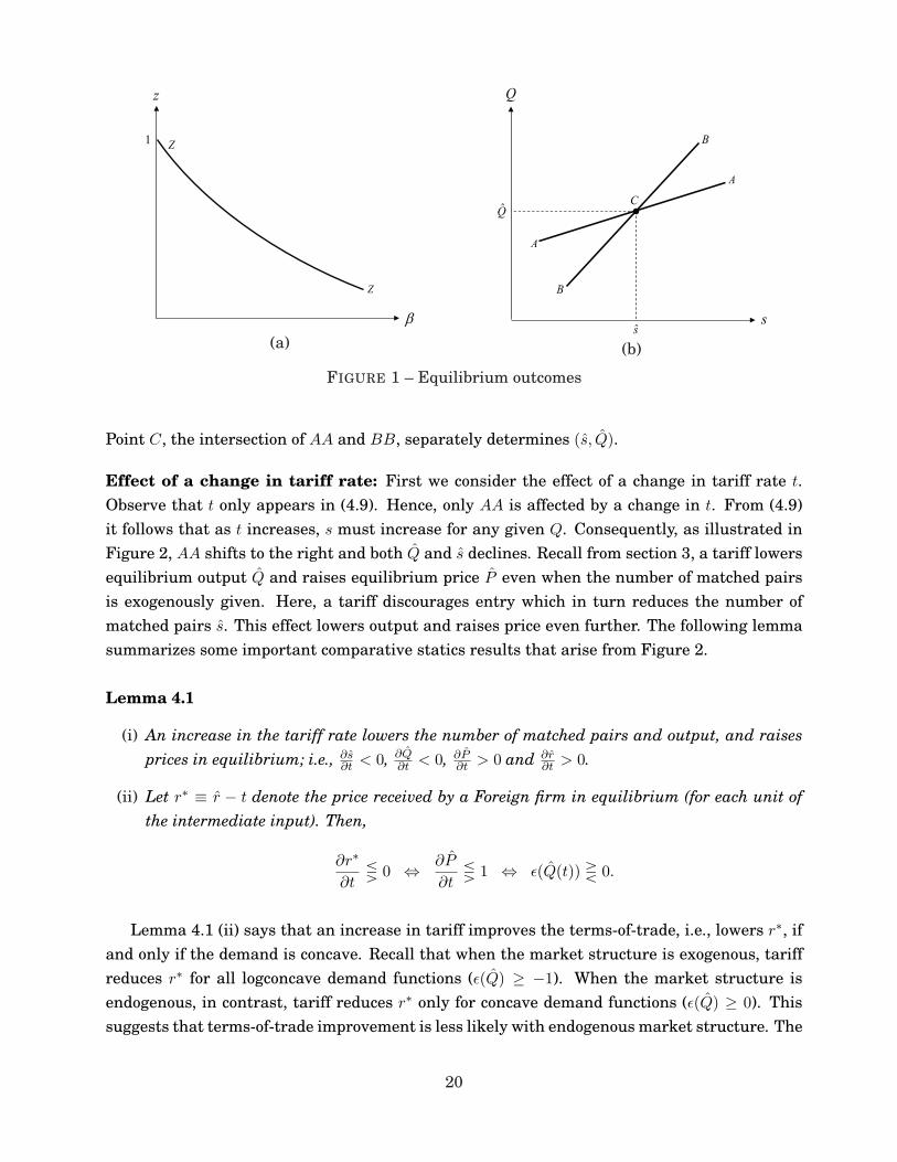
FIGURE 1 – Equilibrium outcomes

Point C, the intersection of AA and BB, separately determines (s, Q).

Effect of a change in tariff rate: First we consider the effect of a change in tariff rate t.Observe that t only appears in (4.9). Hence, only AA is affected by a change in t. From (4.9)it follows that as t increases, s must increase for any given Q. Consequently, as illustrated inFigure 2, AA shifts to the right and both Q and s declines. Recall from section 3, a tariff lowersequilibrium output Q and raises equilibrium price P even when the number of matched pairsis exogenously given. Here, a tariff discourages entry which in turn reduces the number ofmatched pairs s. This effect lowers output and raises price even further. The following lemmasummarizes some important comparative statics results that arise from Figure 2.

Lemma 4.1

(i) An increase in the tariff rate lowers the number of matched pairs and output, and raisesprices in equilibrium; i.e., ∂s

∂t < 0, ∂Q∂t < 0, ∂P

∂t > 0 and ∂r∂t > 0.

(ii) Let r∗ ≡ r − t denote the price received by a Foreign firm in equilibrium (for each unit ofthe intermediate input). Then,

∂r∗

∂tQ 0 ⇔ ∂P

∂tQ 1 ⇔ ε(Q(t)) R 0.

Lemma 4.1 (ii) says that an increase in tariff improves the terms-of-trade, i.e., lowers r∗, ifand only if the demand is concave. Recall that when the market structure is exogenous, tariffreduces r∗ for all logconcave demand functions (ε(Q) ≥ −1). When the market structure isendogenous, in contrast, tariff reduces r∗ only for concave demand functions (ε(Q) ≥ 0). Thissuggests that terms-of-trade improvement is less likely with endogenous market structure. The

20

s

Q

A

A

B

s

Q

B

C 'A

'A

'C

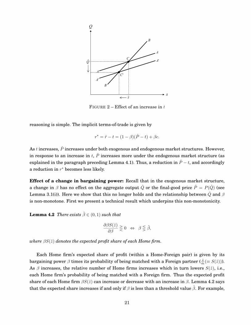
FIGURE 2 – Effect of an increase in t

reasoning is simple. The implicit terms-of-trade is given by

r∗ = r − t = (1− β)(P − t) + βc.

As t increases, P increases under both exogenous and endogenous market structures. However,in response to an increase in t, P increases more under the endogenous market structure (asexplained in the paragraph preceding Lemma 4.1). Thus, a reduction in P − t, and accordinglya reduction in r∗ becomes less likely.

Effect of a change in bargaining power: Recall that in the exogenous market structure,a change in β has no effect on the aggregate output Q or the final-good price P = P (Q) (seeLemma 3.1(i)). Here we show that this no longer holds and the relationship between Q and β

is non-monotone. First we present a technical result which underpins this non-monotonicity.

Lemma 4.2 There exists β ∈ (0, 1) such that

∂βS(z)∂β

R 0 ⇔ β Q β,

where βS(z) denotes the expected profit share of each Home firm.

Each Home firm’s expected share of profit (within a Home-Foreign pair) is given by itsbargaining power β times its probability of being matched with a Foreign partner ( s

m(≡ S(z))).As β increases, the relative number of Home firms increases which in turn lowers S(z), i.e.,each Home firm’s probability of being matched with a Foreign firm. Thus the expected profitshare of each Home firm βS(z) can increase or decrease with an increase in β. Lemma 4.2 saysthat the expected share increases if and only if β is less than a threshold value β. For example,

21

s

Q

A

A

B

s

Q

B

C

'B

'B

'C

(a)

s

Q

A

A

B

s

Q

B

C

'B

'B

'C

(b)

FIGURE 3 – Effect of an increase in β

consider β < β. From Lemma 4.2 we know that βS(z) increases as β increases in this range.From (4.10) it follows that, for a given Q, s must increase. Thus BB shifts to the right andconsequently both Q and s increase. Exactly the opposite holds when β > β. Figures 3(a) and3(b) respectively illustrate the effect of an increase in β when β < β and β > β.

The discussion above implies the following non-monotonicity result.

Lemma 4.3 The relationship between aggregate output Q and bargaining power β is non-monotone. In particular, there exists β such that

∂Q

∂βR 0 ⇔ β Q β.

A similar non-monotone relationship holds between the number of matched pairs s and β.

To better appreciate the non-monotone relationship between Q and β, suppose KH = KF

and β is low. It follows from (4.11) that m < n, i.e., there are fewer Home firms. An increase inβ encourages entry by Home firms and prompts exit by Foreign firms. This improves matching(because there were fewer Home firms to start with) and leads to an increase in the aggregateoutput. On the other hand, if β is high to start with, m > n. By inducing the entry of Homefirms and the exit of Foreign firms, a further increase in β worsens the mismatch which inturn leads to lower aggregate output. As we show in the next subsection, the non-monotonerelationship between Q and β carries over to the non-monotone relationship between optimaltariff t and β. The particular nature of non-monotonicity, however, depends on the curvature ofthe demand function.

22

4.3 Tariffs

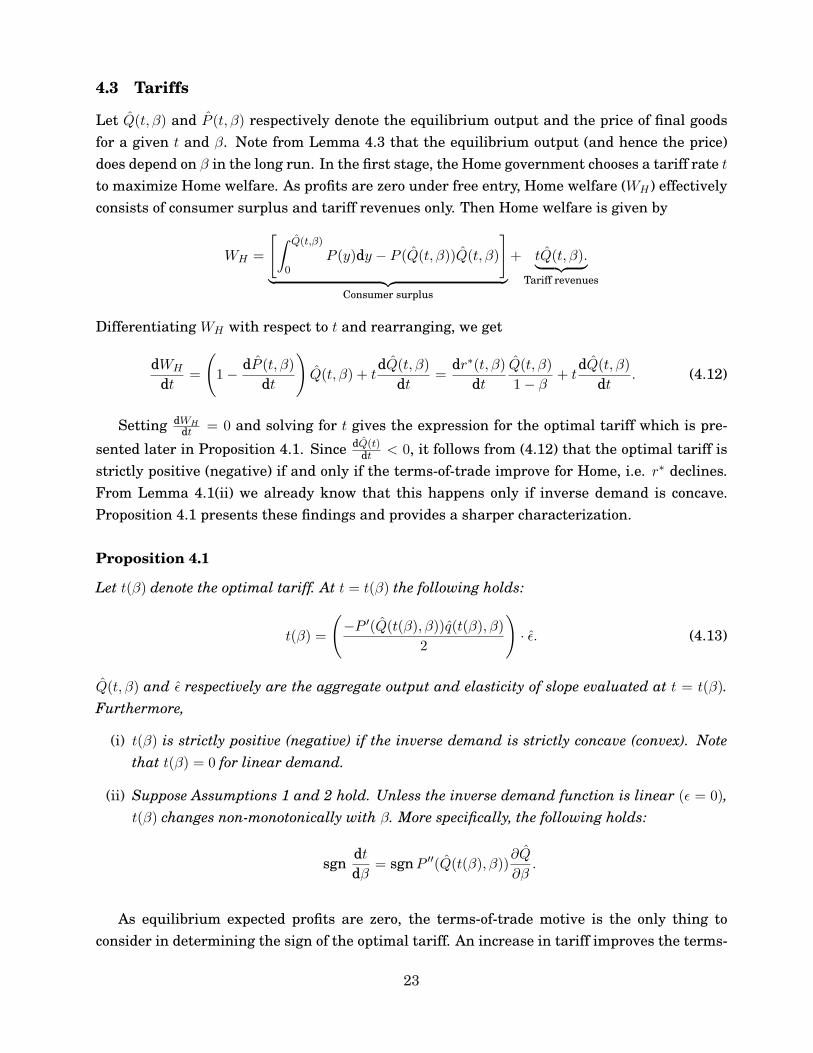
Let Q(t, β) and P (t, β) respectively denote the equilibrium output and the price of final goodsfor a given t and β. Note from Lemma 4.3 that the equilibrium output (and hence the price)does depend on β in the long run. In the first stage, the Home government chooses a tariff rate t

to maximize Home welfare. As profits are zero under free entry, Home welfare (WH ) effectivelyconsists of consumer surplus and tariff revenues only. Then Home welfare is given by

WH =

[∫ Q(t,β)

0P (y)dy − P (Q(t, β))Q(t, β)

]

︸ ︷︷ ︸Consumer surplus

+ tQ(t, β).︸ ︷︷ ︸Tariff revenues

Differentiating WH with respect to t and rearranging, we get

dWH

dt=

(1− dP (t, β)

dt

)Q(t, β) + t

dQ(t, β)dt

=dr∗(t, β)

dt

Q(t, β)1− β

+ tdQ(t, β)

dt. (4.12)

Setting dWHdt = 0 and solving for t gives the expression for the optimal tariff which is pre-

sented later in Proposition 4.1. Since dQ(t)dt < 0, it follows from (4.12) that the optimal tariff is

strictly positive (negative) if and only if the terms-of-trade improve for Home, i.e. r∗ declines.From Lemma 4.1(ii) we already know that this happens only if inverse demand is concave.Proposition 4.1 presents these findings and provides a sharper characterization.

Proposition 4.1

Let t(β) denote the optimal tariff. At t = t(β) the following holds:

t(β) =

(−P ′(Q(t(β), β))q(t(β), β)

2

)· ε. (4.13)

Q(t, β) and ε respectively are the aggregate output and elasticity of slope evaluated at t = t(β).Furthermore,

(i) t(β) is strictly positive (negative) if the inverse demand is strictly concave (convex). Notethat t(β) = 0 for linear demand.

(ii) Suppose Assumptions 1 and 2 hold. Unless the inverse demand function is linear (ε = 0),t(β) changes non-monotonically with β. More specifically, the following holds:

sgndt

dβ= sgn P ′′(Q(t(β), β))

∂Q

∂β.

As equilibrium expected profits are zero, the terms-of-trade motive is the only thing toconsider in determining the sign of the optimal tariff. An increase in tariff improves the terms-

23

)(t

1

0

21

1d

1d

1d

FIGURE 4 – Non-monotonicity of t(β)

of-trade if and only if the demand is concave, which explains Proposition 4.1(i): the optimalpolicy is tariff (subsidy) with strictly concave (convex) demand functions.

What should we make of the fact that (a) demand curvature matters for the sign of theoptimal tariff and (b) the relationship between bargaining power and tariff differs betweenthe two cases – endogenous and exogenous market structures? Our reading of the literaturesuggests that, in terms of the dependence of optimal policy on demand curvature, our resultshave a similar flavor to some of the existing results in the trade literature. For example, theclassic result that the sign of the optimal tariff in the presence of a foreign monopoly dependson whether there is incomplete pass-through, which in turn depends on whether the demandcurve is flatter than the marginal revenue curve (Brander and Spencer, 1984a,b; Helpman andKrugman, 1989, Chapter 4). Concerning the difference in results between endogenous andexogenous market structures, our finding is in the line with Horstmann and Markusen (1986)and Venables (1985), who have shown that in the single-stage oligopoly models, entry can alteroptimal trade policy due to firm-delocation effects. This point has also recently been made byEtro (2011) and Bagwell and Staiger (2012a, b) in the contexts of strategic trade policy andtrade agreements respectively. We do not necessarily view (b) as a shortcoming. Depending onthe industry characteristics, such as industry-specific fixed costs or stability of demand, someindustries fit an exogenous market structure description better, while for some other industrieswith fluid entry and volatile demand, an endogenous market structure is more apt.

Proposition 4.1(ii) suggests that the relationship between t and β depends crucially on howthe aggregate output, Q, varies with β and also on the curvatures of inverse demand and itsslope. As Q varies non-monotonically with β the relationship between t and β is non-monotone.

To see the non-monotonicity clearly, consider once again P (Q) = a − Qd, d > 0. SupposeKH = KF , and s(m, n) = mn

m+n which implies S(z) = z1+z . Then, according to Proposition 4.1,

24

for concave demand (d > 1), the optimal tariff t(β) initially declines as β increases, becominglowest at equal bargaining power (i.e., β = 1

2 ), and then increases as β increases further. Forconvex demand (d < 1), the relationship between β and t(β) is exactly the opposite. If thedemand is linear, i.e., d = 1, t(β) = 0 for β ∈ [0, 1]. Figure 4 illustrates the relationship betweenβ and t(β). We conclude by noting that the non-monotonicity of t(β) is in fact more general.

Proposition 4.2 Consider all inverse demand functions P (Q) that satisfy Assumptions 1 and 2,and are either concave for all Q ≥ 0 or convex for all Q ≥ 0. The relationship between t and β isU-shaped (inverted U-shaped) if the demand function is strictly concave (convex). If the demandfunction is linear, free trade is optimal (i.e., optimal tariff is zero) irrespective of the bargainingpower.

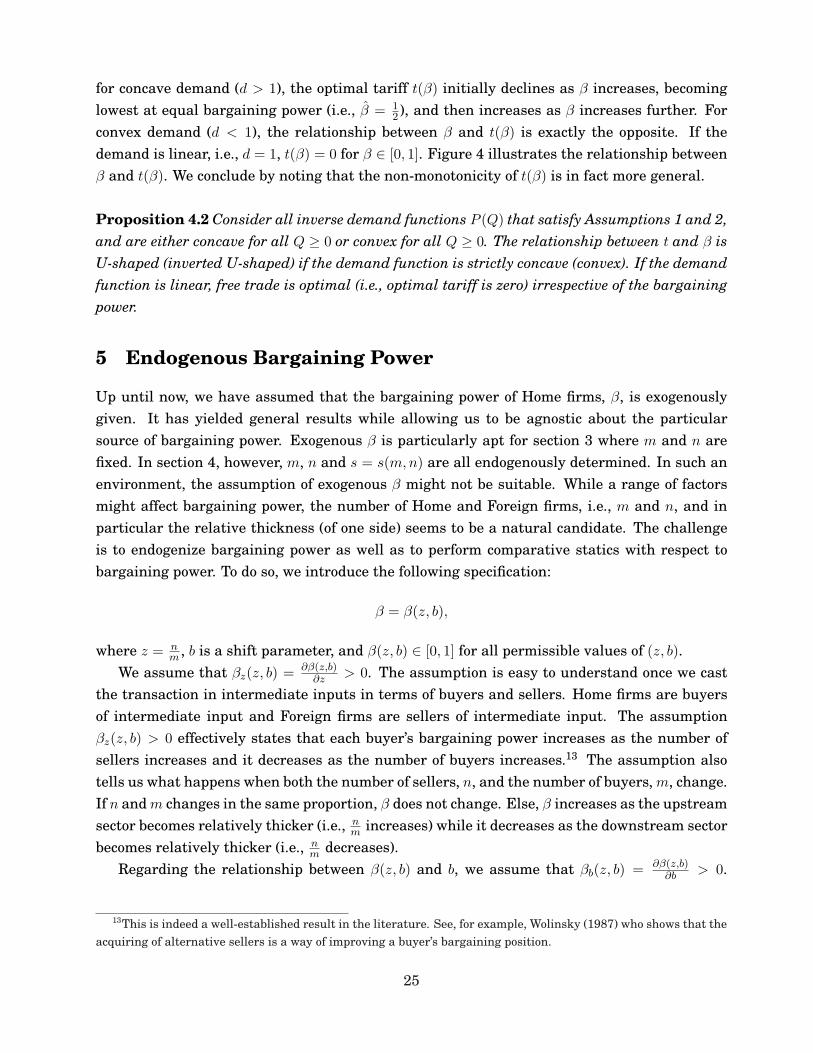
5 Endogenous Bargaining Power

Up until now, we have assumed that the bargaining power of Home firms, β, is exogenouslygiven. It has yielded general results while allowing us to be agnostic about the particularsource of bargaining power. Exogenous β is particularly apt for section 3 where m and n arefixed. In section 4, however, m, n and s = s(m,n) are all endogenously determined. In such anenvironment, the assumption of exogenous β might not be suitable. While a range of factorsmight affect bargaining power, the number of Home and Foreign firms, i.e., m and n, and inparticular the relative thickness (of one side) seems to be a natural candidate. The challengeis to endogenize bargaining power as well as to perform comparative statics with respect tobargaining power. To do so, we introduce the following specification:

β = β(z, b),

where z = nm , b is a shift parameter, and β(z, b) ∈ [0, 1] for all permissible values of (z, b).

We assume that βz(z, b) = ∂β(z,b)∂z > 0. The assumption is easy to understand once we cast

the transaction in intermediate inputs in terms of buyers and sellers. Home firms are buyersof intermediate input and Foreign firms are sellers of intermediate input. The assumptionβz(z, b) > 0 effectively states that each buyer’s bargaining power increases as the number ofsellers increases and it decreases as the number of buyers increases.13 The assumption alsotells us what happens when both the number of sellers, n, and the number of buyers, m, change.If n and m changes in the same proportion, β does not change. Else, β increases as the upstreamsector becomes relatively thicker (i.e., n

m increases) while it decreases as the downstream sectorbecomes relatively thicker (i.e., n

m decreases).Regarding the relationship between β(z, b) and b, we assume that βb(z, b) = ∂β(z,b)

∂b > 0.

13This is indeed a well-established result in the literature. See, for example, Wolinsky (1987) who shows that theacquiring of alternative sellers is a way of improving a buyer’s bargaining position.

25

z

1 Z

Z

Y

Y

ˆ

z

D

(a)

s

Q

A

A

B

s

Q

B

C

(b)

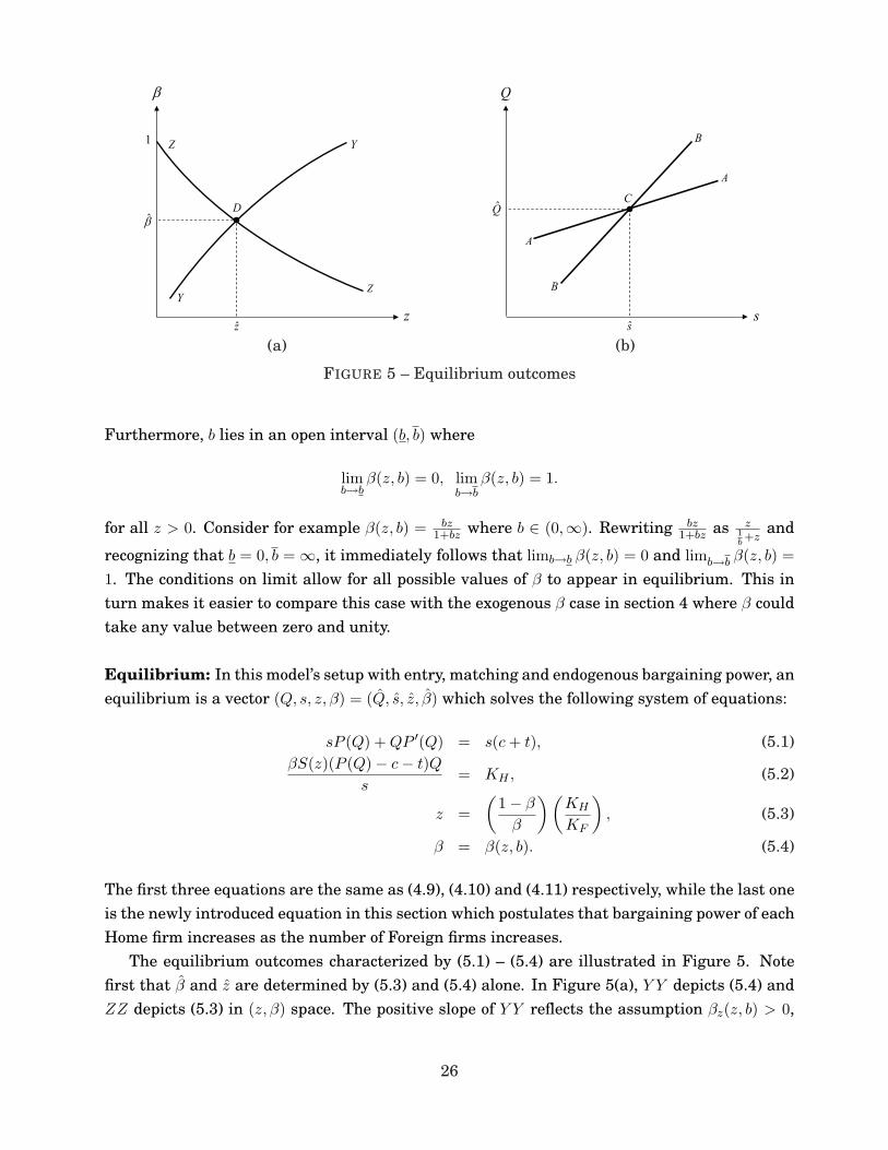
FIGURE 5 – Equilibrium outcomes

Furthermore, b lies in an open interval (b, b) where

limb→b

β(z, b) = 0, limb→b

β(z, b) = 1.

for all z > 0. Consider for example β(z, b) = bz1+bz where b ∈ (0,∞). Rewriting bz

1+bz as z1b+z

and

recognizing that b = 0, b = ∞, it immediately follows that limb→b β(z, b) = 0 and limb→b β(z, b) =1. The conditions on limit allow for all possible values of β to appear in equilibrium. This inturn makes it easier to compare this case with the exogenous β case in section 4 where β couldtake any value between zero and unity.

Equilibrium: In this model’s setup with entry, matching and endogenous bargaining power, anequilibrium is a vector (Q, s, z, β) = (Q, s, z, β) which solves the following system of equations:

sP (Q) + QP ′(Q) = s(c + t), (5.1)βS(z)(P (Q)− c− t)Q

s= KH , (5.2)

z =(

1− β

β

)(KH

KF

), (5.3)

β = β(z, b). (5.4)

The first three equations are the same as (4.9), (4.10) and (4.11) respectively, while the last oneis the newly introduced equation in this section which postulates that bargaining power of eachHome firm increases as the number of Foreign firms increases.

The equilibrium outcomes characterized by (5.1) – (5.4) are illustrated in Figure 5. Notefirst that β and z are determined by (5.3) and (5.4) alone. In Figure 5(a), Y Y depicts (5.4) andZZ depicts (5.3) in (z, β) space. The positive slope of Y Y reflects the assumption βz(z, b) > 0,

26

z

1 Z

Z

Y

Y

ˆ

z

'Y

'Y

D

'D

FIGURE 6 – Effect of an increase in b

while the negative slope of ZZ is the same as before. Point D, the intersection of Y Y and ZZ,endogenously determines z and β. Taking (z, β) as given, Figure 5(b) depicts (5.1) and (5.2)which are given by AA and BB. As in Figure 4(b), Point C separately determines Q and s.

Comparative statics: The effect of a change in tariff is the same as before. From (5.3) and(5.4), a change in t does not affect Y Y or ZZ and it does not affect β. Thus, the effect of tariffon s, Q, P and r with endogenous β is the same as the ones with exogenous β.

What about the effect of a change in the bargaining power parameter b? Since βb(z, b) > 0,an increase in b shifts Y Y upwards, whereas ZZ does not change. As a result β increases (seeFigure 6). Given dβ

db > 0, limb→b β(z, b) = 0 and limb→b β(z, b) = 1, it follows that each β ∈ (0, 1)can be traced to a unique b ∈ (b, b). In particular, there exists a unique b = b that induces β = β

and for all b < (>)b, β < (>)β. The following non-monotonicity results, i.e., Lemmas 5.1(i) and5.1(ii), then immediately follow from Lemmas 4.2 and 4.3 by replacing β with b and replacingβ with b respectively.

Lemma 5.1

(i) There exists b ∈ (0,∞) such that

∂βS(z)∂b

R 0 ⇔ b Q b.

(ii) The relationship between aggregate output Q and b is non-monotone. In particular, thereexists b ∈ (0,∞) such that

∂Q

∂bR 0 ⇔ b Q b.

A similar non-monotone relationship holds between the number of matched pairs s and b.

27

The logic as well as the derivation of optimal tariff are very similar to the ones describedin section 4.3 and hence omitted here. Note that three features are crucial in characterizingoptimal tariff in section 4: (i) z is independent of t; (ii) bargaining power is independent of t (asβ was exogenous); and (iii) there is a non-monotone relationship between Q and β. All threefeatures remain intact in this section. As a result, the characterization of optimal tariff underendogenous β remains effectively the same as the characterization under exogenous β (i.e., asin Proposition 4.1) by replacing β with b.

Proposition 5.1 Let t(b) denote the optimal tariff. At t = t(b) the following holds:

t(b) =

(−P ′(Q(t(b), b))q(t(b), b)

2

)· ε. (5.5)

Q(t, b) and ε respectively are the aggregate output and elasticity of slope evaluated at t = t(b).Furthermore,

(i) t(b) is strictly positive (negative) if the inverse demand is strictly concave (convex). Notethat t(b) = 0 for linear demand.

(ii) Suppose Assumptions 1 and 2 hold. Unless the inverse demand function is linear (ε = 0),t(b) changes non-monotonically with b. More specifically, the following holds:

sgndt

db= sgn P ′′(Q(t(b), b))

∂Q

∂b.

We conclude the section with an example. Consider once again P (Q) = a−Qd and s(m,n) =mn

m+n which respectively yields constant elasticity of slope ε = d − 1 and normalized matchingfunction S(z) = z

1+z where z = nm . Assume β(z, b) = bz

1+bz where b ∈ (0,∞). Furthermore,assume that KH = KF , i.e., k = 1. Using these assumptions and specific functional forms forinverse demand and matching functions we get:

z =1√b, β =

√b

1 +√

b, βS(z) =

√b

(1 +√

b)2.

Note that∂βS(z)

∂b≡ 1−

√b

2(1 +√

b)3√

bR 0 ⇔ b Q 1,

which implies∂Q

∂bR 0 ⇔ b Q 1.

Then, according to Proposition 5.1, for concave demand (d > 1), the optimal tariff t(b) initiallydeclines as b increases, becoming lowest at b = 1 (or β = 1

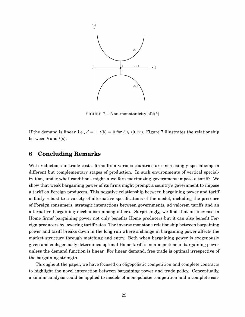
2 ) and then increases as b increasesfurther. For convex demand (d < 1), the relationship between b and t(b) is exactly the opposite.

28

b

)(bt

1

0

1d

1d

1d

FIGURE 7 – Non-monotonicity of t(b)

If the demand is linear, i.e., d = 1, t(b) = 0 for b ∈ (0,∞). Figure 7 illustrates the relationshipbetween b and t(b).

6 Concluding Remarks

With reductions in trade costs, firms from various countries are increasingly specializing indifferent but complementary stages of production. In such environments of vertical special-ization, under what conditions might a welfare maximizing government impose a tariff? Weshow that weak bargaining power of its firms might prompt a country’s government to imposea tariff on Foreign producers. This negative relationship between bargaining power and tariffis fairly robust to a variety of alternative specifications of the model, including the presenceof Foreign consumers, strategic interactions between governments, ad valorem tariffs and analternative bargaining mechanism among others. Surprisingly, we find that an increase inHome firms’ bargaining power not only benefits Home producers but it can also benefit For-eign producers by lowering tariff rates. The inverse monotone relationship between bargainingpower and tariff breaks down in the long run where a change in bargaining power affects themarket structure through matching and entry. Both when bargaining power is exogenouslygiven and endogenously determined optimal Home tariff is non-monotone in bargaining powerunless the demand function is linear. For linear demand, free trade is optimal irrespective ofthe bargaining strength.

Throughout the paper, we have focused on oligopolistic competition and complete contractsto highlight the novel interaction between bargaining power and trade policy. Conceptually,a similar analysis could be applied to models of monopolistic competition and incomplete con-

29

tracts – two features that have been extensively used in the recent literature on outsourcingand vertical specialization (see, e.g., Grossman and Helpman (2002)). Typically, these modelshave relationship-specific investments. Although our model abstracts from such investments,entry plays a similar role in our framework. In a model with relationship-specific investments,an increase in the bargaining power of downstream firms would reduce upstream investments.In a similar spirit, we also find that an increase in the bargaining power of downstream firmsdiscourages entry by upstream firms. Given the similarity in effects of entry and investment,we conjecture that a non-monotone relationship between bargaining power and tariff wouldarise in models with relationship-specific investments.

Finally, we conclude with a remark on cost heterogeneity. While firms with heterogeneouscosts have become an integral part of new trade models with monopolistic competition since theseminal work of Melitz (2003), the implications of cost heterogeneity on trade policy have notbeen adequately explored. In the context of partial equilibrium oligopoly models, Lahiri andOno (2007, Chapter 4) and Long and Soubreyan (1997), for example, have shown that tradeand industrial policies arising from asymmetric oligopoly can be significantly different fromthose arising from symmetric oligopoly. In future work, we plan to incorporate cost asymmetryin oligopoly models with vertical relationships and examine its implication for trade policy.

30

Appendix

A Proofs for Section 3

A.1 Equivalence between Assumptions 1 and 1’The assumption Q(P ) is logconcave implies

ddP

»d ln Q(P )

dP

–=

ddP

»Q′(P )

Q(P )

–

=Q(P ) ·Q′′(P )− [Q′(P )]2

[Q(P )]2≤ 0,

which can be expressed asQ(P )Q′′(P )

[Q′(P )]2≤ 1. (A.1)

Differentiating P = P (Q(P )) with respect to P , we get

1 = P ′(Q(P ))Q′(P ).

Differentiating this once again with respect to P gives

0 = P ′′[Q′(P )]2 + P ′Q′′(P ).

Rewriting this equation, we getQ′′(P )

[Q′(P )]2= −P ′′

P ′.

Substituting this relationship into (A.1), we find that

−QP ′′(Q)

P ′(Q)≤ 1,

which implies P ′(Q) + QP ′′(Q) ≤ 0. ˜

A.2 Proof of Lemma 3.1(i) It immediately follows from noting that Q, i.e., the value of Q that solves (3.3), does not depend on β.(ii) Totally differentiating (3.2) and (3.3) yields

dQ

dt=

s/P ′(Q)

s + 1 + ε(Q),

dP

dt= P ′(Q)

dQ

dt=

s

s + 1 + ε(Q),

dr

dt= (1− β)

dP

dt+ β =

s + β(1 + ε(Q))

s + 1 + ε(Q),

whereε(Q) ≡ P ′′(Q)Q

P ′(Q)

represents the elasticity of the slope of the demand. From Assumption 1’ it follows that ε(Q) ≥ −1, which in turn implies thats + 1 + ε(Q) > 0. The claim directly follows from noting that P ′(Q) < 0 and s + β(1 + ε(Q)) > 0.(iii) We have that

dr∗

dt=

dr

dt− 1 = (1− β)

dP

dt− 1

!= −(1− β)

1 + ε(Q)

s + 1 + ε(Q).

31

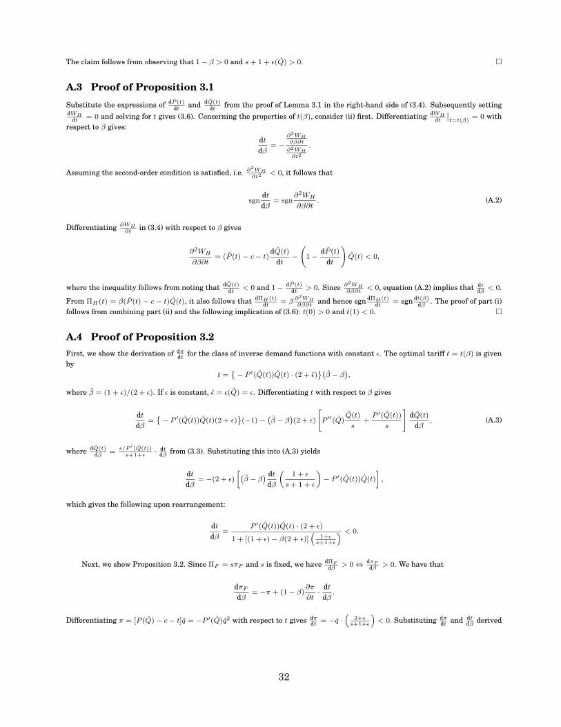
The claim follows from observing that 1− β > 0 and s + 1 + ε(Q) > 0. ˜

A.3 Proof of Proposition 3.1Substitute the expressions of dP (t)

dtand dQ(t)

dtfrom the proof of Lemma 3.1 in the right-hand side of (3.4). Subsequently setting

dWHdt

= 0 and solving for t gives (3.6). Concerning the properties of t(β), consider (ii) first. Differentiating dWHdt

˛t=t(β)

= 0 withrespect to β gives:

dt

dβ= −

∂2WH∂β∂t

∂2WH∂t2

.

Assuming the second-order condition is satisfied, i.e. ∂2WH∂t2

< 0, it follows that

sgndt

dβ= sgn

∂2WH

∂β∂t. (A.2)

Differentiating ∂WH∂t

in (3.4) with respect to β gives

∂2WH

∂β∂t= (P (t)− c− t)

dQ(t)

dt−

1− dP (t)

dt

!Q(t) < 0,

where the inequality follows from noting that dQ(t)dt

< 0 and 1− dP (t)dt

> 0. Since ∂2WH∂β∂t

< 0, equation (A.2) implies that dtdβ

< 0.

From ΠH(t) = β(P (t) − c − t)Q(t), it also follows that dΠH (t)dt

= β ∂2WH∂β∂t

and hence sgn dΠH (t)dt

= sgn dt(β)dβ

. The proof of part (i)follows from combining part (ii) and the following implication of (3.6): t(0) > 0 and t(1) < 0. ˜

A.4 Proof of Proposition 3.2First, we show the derivation of dπ

dtfor the class of inverse demand functions with constant ε. The optimal tariff t = t(β) is given

byt =

˘− P ′(Q(t))Q(t) · (2 + ε)¯`

β − β´,

where β = (1 + ε)/(2 + ε). If ε is constant, ε = ε(Q) = ε. Differentiating t with respect to β gives

dt

dβ=˘− P ′(Q(t))Q(t)(2 + ε)

¯(−1)− `β − β

´(2 + ε)

"P ′′(Q)

Q(t)

s+

P ′(Q(t))

s

#dQ(t)

dβ, (A.3)

where dQ(t)dβ

=s/P ′(Q(t))

s+1+ε· dt

dβfrom (3.3). Substituting this into (A.3) yields

dt

dβ= −(2 + ε)

»`β − β

´ dt

dβ

„1 + ε

s + 1 + ε

«− P ′(Q(t))Q(t)

–,

which gives the following upon rearrangement:

dt

dβ=

P ′(Q(t))Q(t) · (2 + ε)

1 + [(1 + ε)− β(2 + ε)]“

1+εs+1+ε

” < 0.

Next, we show Proposition 3.2. Since ΠF = sπF and s is fixed, we have dΠFdβ

> 0 ⇔ dπFdβ

> 0. We have that

dπF

dβ= −π + (1− β)

∂π

∂t· dt

dβ.

Differentiating π = [P (Q)− c− t]q = −P ′(Q)q2 with respect to t gives dπdt

= −q ·“

2+εs+1+ε

”< 0. Substituting dπ

dtand dt

dβderived

32

above into the above equation, we get

dπF

dβ=

„(2 + ε)π

s + (1− β)(ε + 1)(ε + 2)

«„2 + ε− s

2 + ε− β

«.

The result follows from noting that the value in the first parentheses is strictly positive. ˜

B Proofs for Section 4

B.1 Proof of Lemma 4.1Rewrite the Home firm’s free entry condition (4.10) as

− P ′(Q)Q2

s2=

KH

βS(z). (B.1)

(i) Differentiating (B.1) with respect to t gives∂Q

∂t=

2q

2 + ε· ∂s

∂t. (B.2)

Furthermore, totally differentiating (4.9) with respect to t and rearranging, we get

∂Q

∂t=

s/P ′(Q)

s + 1 + ε+

q

s + 1 + ε

∂s

∂t. (B.3)

Solving (B.2) and (B.3) for ∂s∂t

and ∂Q∂t

yields

∂s

∂t=

„2 + ε

2s + ε

« s

P ′(Q)q

!,

∂Q

∂t=

2s

(2s + ε)P ′(Q),

which in turn gives

∂P

∂t= P ′(Q)

∂Q

∂t=

2s

2s + ε,

∂r

∂t= (1− β)

∂P

∂t+ β =

2s + βε

2s + ε.

The claim follows from observing that 2s + ε > 0, 2s + βs > 0, and P ′(Q) < 0.

(ii) Differentiating r∗ ≡ r − t = (1− β)(P − c− t) + βc with respect to t gives

∂r∗

∂t= (1− β)

∂P

∂t− 1

!= − (1− β)ε

2s + ε.

The claim follows from observing that 1− β > 0 and 2s + ε > 0. ˜

B.2 Proof of Lemma 4.2Defining k = KH

KFwe rewrite (4.11) as z = ( 1

β− 1)k. Thus,

βS(z) = βS

„„1

β− 1

«k

«.

Since both β ∈ (0, 1) and S(z) ∈ (0, 1),

0 ≤ βS

„„1

β− 1

«k

«≤ min

β, S

„„1

β− 1

«k

«ff.

33

We have that limβ→0 β = 0 and limβ→1 S(z) = 0 (by applying (4.7)) which together with the fact that β ≤ 1 and S(z) ≤ 1 implies

limβ→0

βS(z) = 0, limβ→1

βS(z) = 0.

These limit values imply that βS(z) is non-monotone in β. The particular nature of non-monotonicity then follows from noting

that∂βS(( 1

β−1)k)

∂β= k2

β3 S′′(z) < 0, i.e., βS(z) is strictly concave in β. ˜

B.3 Proof of Lemma 4.3The proof is immediate from Lemma 4.2 and the discussion preceding Lemma 4.3. Here we just derive ∂Q

∂βand ∂s

∂βfor future

reference. Differentiating the first-order condition (4.9) with respect to β, we get

∂Q

∂β=

q

s + 1 + ε

∂s

∂β,

where ε ≡ ε(Q(t(β), β)). Similarly, differentiating the Home firm’s free-entry condition (B.1) with respect to β, we get

σ(β)

1− β− 1 = β

2 + ε

Q

∂Q

∂β− 2

s

∂s

∂β

!,

where σ(β) ≡ z(β)S′(z(β))S(z(β))

. Note from (4.8) that σ(β) ∈ (0, 1). Solving the above two equations for ∂Q∂β

and ∂s∂β

gives

∂Q

∂β=

Q

β(2s + ε)

„1− σ(β)

1− β

«,

∂s

∂β=

s(s + 1 + ε)

β(2s + ε)

„1− σ(β)

1− β

«.

The result follows from observing that limβ→0∂Q∂β

> 0, limβ→1∂Q∂β

< 0, limβ→0∂s∂β

> 0, limβ→1∂s∂β

< 0 and P ′(Q) < 0 for allQ ≥ 0. ˜

B.4 Proof of Proposition 4.1Substitute the expressions for dP

dtand dQ

dtfrom proof of Lemma 4.1 in the right-hand side of (4.12). Subsequently setting dWH

dt= 0

and solving for t gives (4.13). The proof of part (i) is immediate from observing (4.13). To see (ii), differentiate dWHdt

˛t=t(β)

= 0

with respect to β which gives:

dt

dβ= −

∂2WH∂β∂t

∂2WH∂t2

.

Since ∂2WH∂t2

< 0 (second-order condition), sgn dtdβ

= sgn ∂2WH∂β∂t

. Differentiating WH with respect to t and simplifying, we get:

dWH

dt=

2st + P ′(Q)Qε

(2s + ε)P ′(Q).

Note from (4.13) that 2st + P ′(Q)Qε = 0 at t = t(β). Differentiating the above equation with respect to β yields:

∂2WH

∂β∂t

˛˛t=t(β)

=2t ∂s

∂β+hQ2P ′′′(Q) + 2QP ′′(Q)

i∂Q∂β

(2s + ε)P ′(Q)(using dt

dβ= 0 at t = t(β))

=

h2t s+1+ε

q+ QP ′′(Q)(2 + α)

i

(2s + ε)P ′(Q)

∂Q

∂β(using ∂s

∂β= s+1+ε

q∂Q∂β

from Lemma 4.3)

=

h−QP ′′(Q)(s + 1 + ε) + QP ′′(Q)(2 + α)

i

(2s + ε)P ′(Q)

∂Q

∂β(using (4.13))

= − ε(s− 1 + ε− α)

2s + ε

∂Q

∂β.

34

where α(Q) ≡ QP ′′′(Q)P ′′(Q)

. Then, the result follows from noting that sgn ε(Q) = −sgn P ′′(Q) (definition of ε(Q)), 2s + ε > 0

(Assumption 1), s− 1 + ε− α > 0 (Assumption 2), and non-monotonicity of ∂Q/∂β (Lemma 4.3). ˜

B.4 Proof of Proposition 4.2The proof is immediate from applying Proposition 4.1 and Lemma 4.3. ˜

35

References[1] ANDERSON, S. P. AND RENAULT, R. (2003): “Efficiency and Surplus Bounds in Cournot Competition.” Journal

of Economic Theory, 113(2), 253-64.

[2] ANTRAS, P. AND ROSSI-HANSBERG, E. (2009): “Organizations and Trade.” Annual Review of Economics, 1,43-64.

[3] ——— AND STAIGER, R. W. (2012a): “Offshoring and the Role of Trade Agreements.” American EconomicReview, 102(7), 3140-83.

[4] ——— AND ——— (2012b): “Trade Agreements and the Nature of Price Determination.” American EconomicReview Papers and Proceedings, 102(3), 470-76.

[5] BAGWELL, K. AND STAIGER, R. W. (2012a): “The Economics of Trade Agreements in the Linear CournotDelocation Model.” Journal of International Economics, 88(1), 32-46.

[6] ——— AND ——— (2012b): “Profit Shifting and Trade Agreements in Imperfectly Competitive Markets.” In-ternational Economic Review, 53(4), 1067-104.

[7] BLANCHARD, E. (2007): “Foreign Direct Investment, Endogenous Tariffs, and Preferential Trade Agreements.”The B.E. Journal of Economic Analysis & Policy, 7(1), [Advances].

[8] ——— (2010): “Reevaluating the Role of Trade Agreements: Does Investment Globalization Make the WTOObsolete?” Journal of International Economics, 82(1), 63-72.

[9] ——— AND MATSCHKE, X. (forthcoming): “U.S. Multinationals and Preferential Market Access.” Review ofEconomics and Statistics.

[10] BRANDER, J. A. AND SPENCER, B. J. (1984a): “Trade and Welfare: Tariffs and Cartels.” Journal of Interna-tional Economics, 16(3-4), 227-42.

[11] ——— AND ——— (1984b): “Tariff Protection and Imperfect Competition.” In Monopolistic Competition andProduct Differentiation and International Trade, edited by Kierzkowski, H., Oxford: Oxford University Press,1984, 194-207.

[12] ——— AND ——— (1985): “Export Subsidies and International Market Share Rivalry.” Journal of Interna-tional Economics, 18, 83-100.

[13] CHEN, Y., ISHIKAWA, J. AND YU, Z. (2004): “Trade Liberalization and Strategic Outsourcing.” Journal ofInternational Economics, 63(2), 419-36.

[14] COLE, M. T. AND DAVIES, R. B. (2011): “Strategic Tariffs, Tariff Jumping, and Heterogeneous Firms.” Euro-pean Economic Review, 55(4), 480-96.

[15] COSTINOT, A. (2009): “An Elementary Theory of Comparative Advantage.” Econometrica, 77(4), 1165-92.

[16] COWAN, S. (2007): “The Welfare Effects of Third-Degree Price Discrimination with Nonlinear Demand Func-tions.” RAND Journal of Economics, 38(2), 419-28.

[17] DENECKERE, R. AND KOVENOCK, D. (1999): “Direct Demand-Based Cournot Existence and Uniqueness Con-ditions.” Mimeo.

[18] ETRO,F. (2011): “Endogenous Market Structures and Strategic Trade Policy.” International Economic Review,52(1), 63-84.

[19] GROSSMAN, G. M. AND HELPMAN, E. (2002): “Integration Versus Outsourcing in Industry Equilibrium.”Quarterly Journal of Economics, 117(1), 85-120.

[20] HANSON, G. H., MATALONI, R. J., AND SLAUGHTER, M. J. (2005): “Vertical Production Networks in Multi-national Firms.” Review of Economics and Statistics, 87(4), 664-78.

[21] HASAN, R., MITRA, D., AND RAMASWAMY, K.V. (2007): “Trade Reforms, Labor Regulations, and Labor-Demand Elasticities: Empirical Evidence from India.” Review of Economics and Statistics, 89(3), 466-81.

36

[22] HELPMAN, E. AND KRUGMAN, P. (1989): Trade Policy and Market Structure. Cambridge, MA: MIT Press.

[23] HORSTMANN, I. J. AND MARKUSEN, J. R. (1986): “Up the Average Cost Curve: Inefficient Entry and the NewProtectionism.” Journal of International Economics, 20(3-4), 225-47.

[24] HUMMELS, D., ISHII, J. AND YI, K.-M. (2001): “The Nature and Growth of Vertical Specialization in WorldTrade.” Journal of International Economics, 54(1), 75-96.

[25] ISHIKAWA, J. AND LEE, K.-D. (1997): “Backfiring Tariffs in Vertically Related Markets.” Journal of Interna-tional Economics, 42(3-4), 395-423.

[26] ——— AND SPENCER, B. (1999): “Rent-Shifting Export Subsidies with an Imported Intermediate Product.”Journal of International Economics, 48(2), 199-232.

[27] JONES, R., KIERZKOWSKI, H. AND LURONG, C. (2005): “What Does Evidence Tell Us about Fragmentationand Outsourcing?” International Review of Economics and Finance, 14(3), 305-16.

[28] KIMURA, F. AND ANDO, M. (2005): “Two-Dimensional Fragmentation in East Asia: Conceptual Frameworkand Empirics.” International Review of Economics and Finance, 14(3), 317-48.

[29] LAHIRI, S. AND ONO, Y. (2007): Trade and Industrial Policy under International Oligopoly. Cambridge, UK:Cambridge University Press.

[30] LIMAO, N. (2006): “Preferential Trade Agreements as Stumbling Blocks for Multilateral Trade Liberalization:Evidence for the United States.” American Economic Review, 96(3), 896-914.

[31] LONG, N. V. AND SOUBREYAN, A. (1997) “Cost Heterogeneity, Industry Concentration and Strategic TradePolicies.” Journal of International Economics, 43(1-2), 207-20.

[32] MELITZ, M. J. (2003): “The Impact of Trade on Intra-Industry Reallocations and Aggregate Industry Produc-tivity.” Econometrica, 71(6), 1695-725.

[33] NOCKE, V. AND WHINSTON, M. D. (2010): “Dynamic Merger Review.” Journal of Political Economy, 118(6),1201-51.

[34] OLARREAGA, M. AND OZDEN, C. (2005): “AGOA and Apparel: Who Captures the Tariff Rent in the Presenceof Preferential Market Access?” World Economy, 28(1), 63-77.

[35] ORNELAS, E. AND TURNER, J. L. (2008): “Trade Liberalization, Outsourcing, and the Hold-Up Problem.”Journal of International Economics, 74(1), 225-41.

[36] ——— AND ——— (2012): “Protection and International Sourcing.” Economic Journal, 112(559), 26-63.

[37] QIU, L. D. AND SPENCER, B. J. (2002): “Keiretsu and Relationship-Specific Investment: Implications forMarket-Opening Trade Policy.” Journal of International Economics, 58(1), 49-79.

[38] SHIMER, R., AND SMITH, L. (2000): “Assortative Matching and Search.” Econometrica, 68(2), 343-69.

[39] SPENCER, B. J. (2005): “International Outsourcing and Incomplete Contracts.” Canadian Journal of Eco-nomics, 38(4), 1107-135.

[40] ——— AND QIU, L. D. (2001): “Keiretsu and Relationship-Specific Investment: A Barrier to Trade?” Interna-tional Economic Review, 42(4), 871-901.

[41] VENABLES, A. (1985): “Trade and Trade Policy with Imperfect Competition: The Case of Identical Productsand Free Entry.” Journal of International Economics, 19(1-2), 1-19.

[42] WOLINSKY, A. (1987): “Matching, Search and Bargaining.” Journal of Economc Theory, 42(2), 311-33.

[43] YEATS, A. J. (2001): “Just How Big Is Global Production Sharing?” In Fragmentation: New Production Pat-terns in the World Economy, edited by Arndt, S. W. and Kierzkowski, H., New York and Oxford: Oxford Uni-versity Press, 2001, 108-43.

[44] YI, K.-M. (2003): “Can Vertical Specialization Explain the Growth of World Trade?” Journal of PoliticalEconomy, 111(1), 52-102.

37