TOMI NIHTILÄ A SIMULATION TOOL FOR SYNCHRONIZATION OF ...
83
TOMI NIHTILÄ A SIMULATION TOOL FOR SYNCHRONIZATION OF MULTISTATIC RADAR Master of Science Thesis Examiners: Professor Karri Palovuori and Professor Ari Visa. Examiners and topic approved by the Faculty Council of the Faculty of Computing and Electrical Engineering on 4 April 2012.
Transcript of TOMI NIHTILÄ A SIMULATION TOOL FOR SYNCHRONIZATION OF ...

TOMI NIHTILÄA SIMULATION TOOL FOR SYNCHRONIZATIONOF MULTISTATIC RADARMaster of Science Thesis
Examiners: Professor Karri Palovuoriand Professor Ari Visa.Examiners and topic approved by theFaculty Council of the Faculty ofComputing and Electrical Engineeringon 4 April 2012.

II
ABSTRACT
TAMPERE UNIVERSITY OF TECHNOLOGYMaster’s Degree Programme in Electrical EngineeringNIHTILÄ, TOMI : A Simulation Tool for Synchronization of Multistatic RadarMaster of Science Thesis, 74 pagesJune 2012Major: Design of Electronic Circuits and SystemsExaminers: Professor Karri Palovuori and Professor Ari VisaKeywords: radar simulation, synchronization of multistatic radar, pulsed Doppler radar,radar signals
Radar transmits electromagnetic waves and observes its surroundings by listeningto the echoes reflected from objects. Conventional monostatic radar has a trans-mitter and receiver in the same system. The concept is commonly used and theimplementation has many benefits. However, in military applications it is desiredto make radar less visible, and a mean to achieve it is to spatially separate thetransmitter and the electromagnetically invisible passive receiver. Multistatic radarhas a transmitter and several separated receivers. This also allows the observationof targets from several angles which aids detecting targets using stealth techniques.
One of the challenges in implementing multistatic radar is the synchronizationbetween transmitter and receiver which is needed for phase-coherent operation. Ex-treme stability in phase is required for the Doppler processing which is the basisof the efficient digital processing of modern radars. Instability weakens the radarperformance, such as detection probability. Synchronization can be performed usinga separate data link, optical fibers, direct radar signal, or independent periodicallysynchronized clocks at all sites. However, the requirements are very high.
Analyzing various synchronization schemes requires knowledge on the used de-vices and different applications while the topic is somewhat confidential. More gen-eral analysis can be conducted using simulations to analyze only the effects of thesynchronization errors on the detection probability or radar images. This way theresults are not application specific but useful information on the relation betweenthe errors and radar signals can be gathered. Eventually the results can be used toanalyze if certain synchronization mean fulfills the set requirements.
This thesis introduces a MATLAB/Simulink simulation tool which can be usedto model the interferences in synchronization signals and examine the effects. Thetool imitates a general radar construction including illustrative blocks and modularstructure allowing easy future modifications. Models of blocks are mainly ideal so farexcept the reference signal path. A survey for typical characteristics of blocks havebeen also made as a guideline for possible model modifications for more accuratepractical components.

III
TIIVISTELMÄ
TAMPEREEN TEKNILLINEN YLIOPISTOSähkötekniikan koulutusohjelmaNIHTILÄ, TOMI: Monipaikkatutkan synkronoinnin simulointityökaluDiplomityö, 74 sivuaKesäkuu 2012Pääaine: Elektroniikan laitesuunnitteluTarkastajat: Professori Karri Palovuori ja Professori Ari VisaAvainsanat: tutkasimulointi, monipaikkatutkan synkronointi, pulssidopplertutka, tutkasig-naalit
Tutka lähettää sähkömagneettisia aaltoja ja havainnoi ympäristöään kuuntele-malla heijastuvia kaikuja. Perinteisen monostaattisen tutkan lähetin ja vastaan-otin sijaitsevat samassa laitteessa. Toteutus on yleisesti käytetty ja sillä on moniaetuja. Sotilaskäytössä huomaamattomuus on kuitenkin toivottavaa ja eräs keinopäästä siihen on erottaa tutkan lähetin ja sähkömagneettisesti näkymätön passiivi-nen vastaanotin toisistaan. Monipaikkatutkalla on lähetin ja useampia eri paikkoihinsijoitettuja passiivisia vastaanottimia. Tämä mahdollistaa myös kohteiden havain-noinnin useasta suunnasta, mikä auttaa havaitsemaan häivekohteita.
Eräs monipaikkatutkan toteutuksen haasteista on lähettimen ja vastaanottimenvälinen synkronointi, jota tarvitaan vaihekoherenttiin toimintaan. Äärimmäinen vai-hestabiilisuus tarvitaan pulssidopplerprosessointiin, joka on tehokkaan digitaalisenprosessoinnin perusta moderneissa tutkissa. Epästabiilisuus heikentää suorituskykyä,kuten havaitsemistodennäköisyyttä. Synkronointi voidaan toteuttaa erillisellä data-linkillä, optisella kuidulla, suoralla tutkasignaalilla tai erillisillä jaksollisesti tahdis-tetuilla kelloilla. Vaatimukset toteutukselle ovat erittäin tarkat.
Erilaisten synkronointitekniikoiden analysointi vaatii tietämystä käytetyistä lait-teista ja eri sovelluksista, kun aihealue samalla on jossain määrin salassa pidettävä.Yleisempää tarkastelua voidaan kuitenkin tehdä analysoimalla simulaation avullavain synkronoinnin virheiden vaikutusta havaitsemistodennäköisyyteen tai tutkaku-viin. Tulokset eivät ole sovelluskohtaisia, vaan yleispätevä yhteys virheiden ja tu-lossignaalien välille voidaan johtaa. Tämän avulla voidaan myöhemmin analysoidatäyttääkö tietty synkronointitekniikka asetetut vaatimukset.
Tämä työ esittelee MATLAB/Simulink-simulaatiotyökalun, jota voidaan käyt-tää mallintamaan häiriöitä referenssisignaaleissa ja tutkimaan vaikutuksia. Työkalunoudattaa geneeristä tutkan rakennetta ja on toteutettu havainnollisina lohkoina.Modulaarinen rakenne mahdollistaa helpon muokattavuuden jatkokehityksessä. Loh-kojen mallit ovat toistaiseksi pääasiassa ideaalisia lukuunottamatta referenssisig-naaleja. Lohkojen tyypillisistä virheistä on myös tehty yleisselvitys, jonka perus-teella voidaan malleja lähteä tarkentamaan vastaamaan käytännön komponentteja.

IV
PREFACE
I started working at the Department of Signal Processing in Tampere University ofTechnology in 2007 as a research assistant. A summer job prolonged and so did mystudies. Everything ends eventually, luckily this time, since it is time to end myMaster studies with this thesis.
This Master of Science thesis has been executed at the Department of SignalProcessing in 2011-2012. The thesis is part of a research project funded by TheFinnish Defense Forces and one part of the project has concerned radar systems,including multistatic radar.
Many people working for the project have been helpful when I have been workingfor this thesis. Thanks to Multimedia and Data Mining group for interesting coffeeroom talks, if not related to the thesis, often very interesting anyway! Special thanksin our group go to Juha Jylhä for being great help defining the topic and writingthe thesis. Due to the nature of the thesis and definition of the topic many meetingshave taken place where numerous people have helped defining the study, especiallyTimo Lensu and Antti Tuohimaa. Also thanks to Juuso Kaitalo, Jarkko Kylmälä,Seppo Horsmanheimo, and the examiners Karri Palovuori and Ari Visa.
Tampere, Finland23 May 2012
Tomi Nihtilä[email protected]

V
CONTENTS
1. Introduction . . . . . . . . . . . . . . . . . . . . . . . . . . . . . . . . . . . 11.1 Background of the Thesis . . . . . . . . . . . . . . . . . . . . . . . . . 21.2 Objectives of the Thesis . . . . . . . . . . . . . . . . . . . . . . . . . . 31.3 Structure of the Thesis . . . . . . . . . . . . . . . . . . . . . . . . . . . 4
2. Radar Fundamentals . . . . . . . . . . . . . . . . . . . . . . . . . . . . . . . 52.1 The Radar Equation . . . . . . . . . . . . . . . . . . . . . . . . . . . . 62.2 Pulsed Waveform . . . . . . . . . . . . . . . . . . . . . . . . . . . . . . 72.3 Doppler Shift . . . . . . . . . . . . . . . . . . . . . . . . . . . . . . . . 122.4 Pulse Doppler Processing . . . . . . . . . . . . . . . . . . . . . . . . . 152.5 Bandwidth and Range Resolution . . . . . . . . . . . . . . . . . . . . . 182.6 Radar Antenna and Angular Resolution . . . . . . . . . . . . . . . . . 202.7 Bistatic and Multistatic Radar . . . . . . . . . . . . . . . . . . . . . . 22
3. Radar Modeling . . . . . . . . . . . . . . . . . . . . . . . . . . . . . . . . . 243.1 Radar Block Diagram . . . . . . . . . . . . . . . . . . . . . . . . . . . 253.2 Basic Signal Model . . . . . . . . . . . . . . . . . . . . . . . . . . . . . 263.3 Mixer Frequency Translation . . . . . . . . . . . . . . . . . . . . . . . 293.4 Synchronous Detector . . . . . . . . . . . . . . . . . . . . . . . . . . . 313.5 Noise Filters . . . . . . . . . . . . . . . . . . . . . . . . . . . . . . . . 333.6 Oscillator . . . . . . . . . . . . . . . . . . . . . . . . . . . . . . . . . . 35
4. Simulation Environment . . . . . . . . . . . . . . . . . . . . . . . . . . . . . 384.1 Introduction of Simulation Tool . . . . . . . . . . . . . . . . . . . . . . 394.2 Non-Ideal Models . . . . . . . . . . . . . . . . . . . . . . . . . . . . . . 474.3 Moving Target Indication . . . . . . . . . . . . . . . . . . . . . . . . . 52
5. Simulation Results . . . . . . . . . . . . . . . . . . . . . . . . . . . . . . . . 545.1 Simulation Tool Operation . . . . . . . . . . . . . . . . . . . . . . . . 545.2 MTI-Attenuation . . . . . . . . . . . . . . . . . . . . . . . . . . . . . . 63
6. Discussion and Conclusions . . . . . . . . . . . . . . . . . . . . . . . . . . . 70Bibliography . . . . . . . . . . . . . . . . . . . . . . . . . . . . . . . . . . . . 73

VI
LIST OF ABBREVIATIONS
ADC Analog-to-Digital ConverterAM Amplitude ModulationARM Anti-Radiation MissileCPI Coherent Processing IntervalCW Continuous WavedBc Decibels compared to carrierdBd Decibels compared to dipole radiatordBFS Decibels compared to full-scale outputdBi Decibels compared to isotropic radiatorDFT Discrete Fourier TransformENOB Effective Number Of BitsFFT Fast Fourier TransformFIR Finite Impulse ResponseFM Frequency ModulationFMCW Frequency-Modulated Continuous WaveGPS Global Positioning SystemHPRF High Pulse Repetition FrequencyHRR High-Range ResolutionI In-phaseIF Intermediate FrequencyIIR Infinite Impulse ResponseISAR Inverse Synthetic Aperture RadarLNA Low-Noise AmplifierLO Local OscillatorLOS Line of SightLPI Low Propability of InterceptLPRF Low Pulse Repetition FrequencyLSB Least Significant BitMPRF Medium Pulse Repetition FrequencyMTI Moving Target IndicationQ QuadraturePM Phase ModulationPRF Pulse Repetition FrequencyPRI Pulse Repetition IntervalRCS Radar Cross SectionRF Radio FrequencyRMS Root-Mean-Squared (value)SAR Synthetic Aperture RadarSFCW Stepped-Frequency Continuous WaveSINAD Signal-to-Noise-and-Distortion RatioSNR Signal-to-Noise RatioSNR+D Signal-to-Noise-and-Distortion RatioWGN White Gaussian Noise

VII
LIST OF SYMBOLS
Chapter 2
E EnergyPr Received powerPt Transmitted powerR Range of a targetσ Radar Cross Section (RCS) of a targetGt Antenna gainAr Effective aperture area of an antennatint Integration timefc Carrier frequencyτ Pulse widthλc Wavelength of carrierc Speed of lightfPRF Pulse repetition frequencyT Length of signal period in timet Timea(t) Instant amplitude in a function of timeA Peak amplitudeω Angular frequency, ω = 2πfϕ0 Initial phaseARMS Root-Mean-Square (RMS) valuePavg Average powerRohm Electrical resistanceD Duty cycleARMS,sine RMS value of continuous sine wavePavg,sine Average power of continuous sine waveSNR Signal-to-Noise RatioPsignal Signal powerPnoise Noise powerRun Unambiguous rangeRo Range observed by the radarϕd Phase differencefd Doppler frequencyvr Radial velocity of a targetfs Sampling rateδr Range resolutionB Bandwidth of the transmitted waveformNs Number of frequency steps∆f Sampling interval in the frequency domain
VIII
tpmax Maximun round-trip propagation delayθ Azimuth angleϕ Elevation angleRt Bistatic range between transmitter and targetRr Bistatic range between target and receiverL Baseline; distance between transmitter and receiverβ Bistatic angle
Chapter 3
fif Intermediate frequencyflo Local oscillator frequencyfc Carrier frequencyfc − fif Variable frequencya(t) Instant time-dependent amplitudeω Angular frequency, ω0 = 2πf0t Timeϕ Phase angleA(t) Rotating phasor with length Aj Imaginary unitfPRF Pulse repetition frequencyfout Output frequency componentsn,m Integersf1, f2 Arbitrary frequenciessm(t) Information signalAm(t) Amplitude informationϕm Phase informationωm Angular frequency of information signalsc(t) Carrier signalωc Angular frequency of carrier signalsAM(t) Amplitude modulated signalµ Modulation indexωif Angular frequency of IF signalϕif Phase angle of IF signalλc Wavelength of the transmitted RF signalAd Range-dependent amplitudeV (t) Instant time-dependent voltageϵ(t) Nominal frequencyϕ(t) Phase noiseσ Standard deviation∆f(t) Frequency fluctuation

IX
Chapter 4
rif(t) IF reference signalflo Local oscillator frequencyfif IF reference frequencyrvar(t) Variable reference signalfc Carrier frequencyfvar Variable reference frequencyϕs(t) Instant phaseϕFM(t) Phase generated by FM-blockµFM FM modulation indexωFM FM angular frequencyϕn(t) Phase noisepn(t) Signal consisting phase noise and FMωvar Variable reference angular frequencyan(t) Amplitude noise (with mean 1)s(t) Output of Interference and noise blockfout Mixer output frequenciesn,m Integersf1, f2 Arbitrary frequenciesSNRideal Ideal SNR of AD-converterSNRj SNR limited by clock jitterσj Clock jitter RMS valueLdB MTI-attenuation in decibelszn Complex pulse

1
1. INTRODUCTION
Originally the term radar was an acronym for RAdio Detection And Ranging. Asthe name implies, in its very basic form it uses radio waves to detect an objectand determine its location. Different types of radars can be found for a varietyof applications: airplanes, ships, weather forecasting, space technology, defense,security, and even conventional cars. Radar types differ a lot depending on thepurpose. Whether the radar is designed for a moving or fixed platform, observinga car 10 meters away, or a missile 200 kilometers away obviously affects the type,size, power, and the operating parameters of the radar.
Technology related to radars has been a popular topic of research for a long timebecause of its crucial role as a main sensor in many applications. The importanceof radar in military applications has been remarkable to hasten its technologicaldevelopment but it also has an essential function in aviation and weather forecast-ing. Vast amount of resources used for radar research has made it rather complexinterdisciplinary device over time. Furthermore, the recent rapid development oftechnology, especially in the field of digital signal processing, has significantly im-proved the performance of radars but has also made them much more complicated.However, the principle of the operation remains the same.
Radar transmits electromagnetic waves via its antenna and observes its surround-ings by listening to the echoes reflected from objects around. The strength of thereflections depends on the average transmitting power of the radar as well as adistance, size, shape, and materials of the object. The intensity of a propagatingelectromagnetic wave attenuates due to the spreading of the energy and the atmo-spheric attenuation. Furthermore, only a small part of the energy scatters backfrom the object to the direction of the measuring antenna. The same phenomenonoccurs for all the obstacles and surfaces the propagating waves encounter generatinginfinite amount of signals summed together with different amplitude, phase, timeand frequency characteristics. A challenging task of radar is to capture this signaland detect the possible objects of interest. Despite the often extremely weak in-teresting signal interfered with strong ground clutter, a term referring uninterestingreflections, and other electromagnetic interference, with the help of careful designand effective signal processing this task is possible.
Processing capabilities of radar are particularly important in the military field

1. Introduction 2
since the task of the radar is to see as much as possible while not to be seen byhostile sensors. This leads to the restriction of radiated power while the receiver hasto perform effective processing methods to be able to deal with the extremely weaksignal returns. Another way to make a radar less visible is to use bistatic radarwhere the transmitter and receiver are located at the different sites, or multistaticradar where the setup has several receivers, and sometimes several transmitters aswell, at different sites. [21, pp. 525-534]
1.1 Background of the Thesis
The advantages of multistatic radar are the electromagnetic invisibility of passivereceivers and new perspectives for seeing targets. Passive receivers are more difficultto detect and destroy and thus can be located closer to the hostile ground in militaryapplications. As they are also cheaper, several of them can be used to gain redun-dancy and to offer new perspectives which helps to detect stealth targets. Theyare designed to absorb some of the electromagnetic energy but mostly they just re-flect the energy to other directions than the direction of arrival of the radar waves.This makes them difficult to detect with monostatic radar but multistatic radarhas several receivers at different directions to detect the scattered energy. However,multistatic radars have some constraints and challenges in implementation and sofar not many operational devices exist. [23, pp. 1-58] [21, pp. 525-534]
Oscillators and timing have crucial role in radar. Timing is needed for calculatingsignal propagation delays for range measurement. Accurate and very stable oscilla-tors are needed for phase-coherent operation to effectively process the received weaksignals. Digital circuits in modern radars also need stable clock signals. Unstablephase causes more noise and ineffective processing which eventually leads to de-creased detection probability in surveillance radar or poor image quality in imagingradars. Timing circuits are drawn in simplified radar block diagram in Figure 1.1where it can be seen that they are connected to all parts of the radar. However,in bistatic or multistatic configuration the parts are not located at the same site sothe synchronization between the sites is needed. Modern rubidium and even quartzclocks are very accurate [23, pp. 258-259] and provide so stable time basis for ap-plications that measuring the errors and instabilities requires special means [14, 15].However, phase-coherent radar, especially in imaging applications, sets extremelyhigh requirements for stability that no stand-alone clock system is enough withoutat least periodical synchronization between the transmitter and receiver [25, 4].
The original objective of the study was to analyze and compare synchronizationmeans for multistatic radar. Synchronization can be implemented for example usingthe transmitted signal from the transmitter via land line, communication link, ordirect signal propagation if line of sight exists between the transmitter and receiver.

1. Introduction 3
Figure 1.1: Simplified radar block diagram.
Periodically synchronized stable clocks on transmitter and receiver sites can be alsoused. One option for external synchronization signal is GPS [28] but at least inmilitary applications it cannot be the only mean. [23, pp. 258-264], [28]
After literature survey and meeting with experts of the field it turned that com-parison of synchronization means is a challenging task and requires lots of back-ground work for comprehensive realization. Due to the lack of practical devicesand the confidential nature of the potentially very effective operational systems notmany documents and reports regarding to the systems exist, although, there aretechnical and scientific interest on multistatic radar and the amount of publicationsis growing. However, a decision was made to develop a tool for future analysis.With the tool, the errors and interferences in the synchronization and their effect onthe radar signals, and with careful analysis the effect on the detection probabilityin a surveillance radar or the quality of the images in an imaging radar, can beexamined. Thus, later when the specifications of the specific synchronization meansof interest are known simulations can be made to analyze if the method fulfills theperformance requirements.
1.2 Objectives of the Thesis
This thesis introduces an approach to simulate radar by modeling a radar transmit-ter and receiver and signals between them. Focus is on a multistatic setup wherethe transmitter and receivers are not located at the same site. Thus, the signalreferences and timing, or synchronization, between the transmitter and receiversneed to be carefully considered. A simulation tool has been developed using MAT-LAB/Simulink software to analyze how noise and distortion in the transmission pathof the synchronization signals affect the receiver performance and eventually, for ex-ample, detection probability. The simulation has been built from the beginning buta way to model high range-resolution radar in Simulink has been published in [6].High range-resolution imaging radar is also an application of interest to model with

1. Introduction 4
the simulation tool and to examine how interferences affect the quality of the images.The simulation tool can model different types of errors in the synchronization
path but many other parts are considered as ideal devices. However, due to theillustrative block diagram representation and modular structure of the simulationmodel it is rather easy to modify it to meet the desired level of modeling accuracy.The ideal models of components can be modified to imitate practical componentswith typical errors and nonlinearities, although, it needs time and knowledge to ver-ify and validate these models. However, brief survey to some typical characteristicsof radar components have been made. The simulated errors rely on the ones thatcan be verified using literature. If possible the results will be compared to the resultsof a real measurement radar.
The objective is to develop a simulation tool to model radar and at this pointfocus on the synchronization and reference signals of the radar, and also to under-stand the limitations and practical characteristics of components the simulation toollacks. With this tool it is possible to model interferences and distortions and analyzetheir effect on the receiver performance, whether it is the detection probability ofsurveillance radar or image quality of an imaging radar. The simulations can be usedfor assessing and developing different radar concepts, especially when determiningthe cause-and-effect relationship of their low-level solutions to their high-level per-formance. The simulation tool can be also used to better understand the low-leveloperation of radar and examine what are the interference-sensitive parts. This wayit can be possible to assess which are the components worth using resources to tweakthe performance.
1.3 Structure of the Thesis
Chapter 2 introduces general radar theory and operating parameters emphasizingon a pulsed radar. Doppler processing and the concepts of bistatic and multistaticradar are presented. Chapter 3 continues radar theory inside the radar with a blockdiagram and describes the main components of radar. Some signal theory, models,and representations are introduced which are useful for the simulation. Finallyoscillator and its possible interferences are explained as a basis for the simulationinterference modeling. The theory in Chapter 3 is the basis for the implementationof the simulation tool.
Chapter 4 introduces the developed simulation tool block by block and ideasfor future expansions of the used models. Chapter 5 presents the operation ofthe simulation tool by graphical illustrations and verifications of the implementedfeatures as a results of the thesis.
Chapter 6 concludes the thesis by assessing the applicability of the simulationtool. Future development is considered and several prospects are suggested.
5
2. RADAR FUNDAMENTALS
Radar consists of an antenna, transmitter, and receiver, from which especially thelatter two can be further divided into many smaller subsystems. In a conventionalmonostatic radar all these are located at the same site. This type of radar time-interleaves the use of the antenna for the transmitter and receiver; when the radartransmits it cannot receive and vice versa. In a bistatic configuration, the trans-mitter and receiver are spatially separated with their own antennas, setting newopportunities but also challenges. A multistatic radar is an expansion of the bistaticradar and contains several receiver antennas at different locations. [21, pp. 3-14]
Radars can also be divided into two main types based on the waveform: continu-ous wave (CW) and pulsed radars. A CW radar transmits the signal via its antennacontinuously while listening to the echoes with another antenna. By sensing theDoppler shift caused by a moving target on the transmitted wave, the radar candetermine the speed of the target. A conventional pulsed radar transmits a series ofrelatively narrow rectangular-like pulses and listens to the echoes between the pulsesusing the same antenna for transmission and reception. This type of radar can alsosense Doppler shifts with some constraints. Pulsed operation not only prevents thehigh-power transmitter from interfering with the sensitive receiver but also allowsstraightforward range measurement. [21, pp. 3-14]
The fundamental feature of conventional pulsed radar is the ability to measurethe range from the radar to a target by determining the propagation delay of a pulsetraveling at a known speed, the speed of light. One of the basic features of radar isalso a measurement of radial velocity, which is the component of the target velocitytoward the radar, and it can be performed by sensing a Doppler shift or trackingthe rate of change of range over a period of time. To determine the location of atarget, along with its range also the angular direction of the target echo needs to bedetermined. This is done by using a scanning antenna with a narrow beamwidth tofind the maxima of the target reflection. [21, pp. 3-14]
This thesis presents the properties and modeling of radar concentrating on a mul-tistatic configuration. However, basic radar theory and signal models are applicablefor all types of radar and are discussed in Chapters 2 and 3, respectively. The mostessential references providing the background of the thesis are [21, 20, 11, 10, 8].

2. Radar Fundamentals 6
2.1 The Radar Equation
The strength of the echoes of the transmitted waves depends on the average trans-mitting power and a distance, size, shape and materials of the object, and lossesalso exist in different parts of the signal path. All these factors are put together inthe radar equation, sometimes also called the range equation. It is not practical tocalculate actual numerical values with it and it also lacks atmospheric attenuationand other losses, but it is useful for presenting dependencies between simple butimportant factors on the signal propagation path. By the radar equation, receivedsignal energy
E =PtGt
4πR2
σ
4πR2Artint. (2.1)
It has been divided into four factors to represent the physical quantities. In theright side, the leftmost factor is the average power density at a distance R from theradar that radiates average power Pt via an antenna of gain Gt. The second factorrepresents the average power reflected back to the direction of the radar, σ beingthe RCS (Radar Cross Section) of the target, described below. The product of thefirst two factors is the power per unit area returned to the radar antenna having aneffective area Ar. The first three factors multiplied equals to the average receivedecho power Pr by the antenna. Average power multiplied by integration time tint
results in the signal energy E, although, in practice integration is not perfect andsome loss occurs. Signal power and energy are further discussed in Section 2.2 andintegration in Section 2.4. However, it is worth noticing that the received energyis inversely proportional to the fourth power of the range when assuming RCS inquestion to be invariant regarding the range. Hence radar receiver must have veryhigh dynamic range. [20, pp. 1.10-1.12], [21, pp. 135-149]
Whether the received energy is sufficient for a detection further depends on thenoise level and on the processing capabilities of the receiver, briefly discussed inSection 2.4. Moreover, RCS of a typical target tends to fluctuate significantly overtime due to changes in the aspect angle. RCS describes the effective area of thetarget and is a function of wavelength. However, only a sphere has a constant RCSat a certain wavelength while the RCS of a real target is a function of aspect angleand also depends on the material, shape and size (compared to wavelength) of thetarget. Real objects contain different materials and also the observed shape and sizeof the object varies depending on the angle of view. Some shapes tend to concentratethe reflections on the direction of arrival while others reflect the waves away whichis preferred in stealth targets. Furthermore, an echo to a particular direction is asuperposition of waves reflected from different parts of the object. Hence the RCS ina function of aspect angle may vary 20 dB or even 30 dB. This variation, observedtypically from scan-to-scan, is called glint, scintillation, or fluctuation. RCS also

2. Radar Fundamentals 7
Figure 2.1: Pulse train parameters in time domain. Dashed lines indicate the phasecoherence of consecutive pulses compared to the continuous wave which usually holds true.
has different characteristics for clutter, for example the RCS of volumetric clutterincreases by second power of the range. More information and example figures ofRCS can be read in [20, pp. 14.1-14.36].
2.2 Pulsed Waveform
Pulsed radar transmits pulse train with a certain pulse width, pulse repetition fre-quency (PRF), and peak power. Pulses are formed of a radio frequency (RF) carrierwave. PRF fPRF, carrier frequency fc, pulse width τ , and other signal notationsdescribed below are illustrated in time domain in Figure 2.1. Top wave is the con-tinuous sine wave which is modulated by the square wave below it generating pulsesof sine wave seen on the bottom waveform. Corresponding operation is performedin a radar transmitter. More signal parameters and representations are discussed inChapter 3 but some signal nomenclature and parameters are introduced here. [21,pp. 107-114]
Signal Strength
Sine signal with a maximum amplitude of A, frequency f (Hz), angular frequencyω = 2πf (rad/s) and initial angle ϕ0 can be represented as
a(t) = A sin (ωt+ ϕ0), (2.2)

2. Radar Fundamentals 8
where a(t) is the instant amplitude or magnitude of the signal, varying in a functionof time t and is limited between −A and A. An electromagnetic wave propagatesin space at a speed of light c (the speed in air is slightly slower but the differenceis insignificant in this study). While period T = 1/f is the length of one period intime, wavelength λ is the length in distance: λ = c/f . These parameters are shownin Figure 2.1 along with some other signal parameters. [26]
Another important parameter of a periodic signal, especially in electrical engi-neering, is the root-mean-square (RMS) value and it is defined as the name implies
ARMS =
√1
T
∫ t+T
t
a2(t) dt. (2.3)
Varying AC (Alternating Current) signal with RMS value of ARMS volts producesthe same power in a resistance as the constant DC (Direct Current) signal of ARMS
volts. Therefore, for DC signal the RMS value equals the (constant) amplitude ofthe signal, as can be noticed if a(t) in Equation (2.3) is constant. Hence RMS valueis related to the average power
Pavg =A2
RMS
Rohm=
1T
∫ t+T
ta2(t) dt
Rohm. (2.4)
Solving Equations (2.3) and (2.4) for sine wave gives ARMS,sine = A/√2 and Pavg,sine =
12A2/Rohm. In communications engineering Rohm is often considered to be 1 ohm
since it may be difficult to know the actual value and in signal comparisons itdoes not even matter. Hence it is often excluded in equations. When using the1-ohm convention, amplitude squared can be considered as the instantaneous powerPinst = a2(t). Integrating instantaneous power over time results in energy, and aver-aging it over time gives the average power, as is seen in Equation (2.3). [12, 5, 26]
The frequency of the pulse train, or the rate of pulses to be exact, in radar equalsfPRF (Figure 2.1) and average power can be defined using duty cycle D = τ/T =
τfPRF and peak power. The power of the sine wave in Figure 2.1 is Pavg,sine =12A2
(when the resistance is excluded) and the average power of a pulse train of sine wavepulses seen on the bottom in Figure 2.1 is
Pavg = DPavg,sine =1
2τfPRFA
2. (2.5)
To be exact, an assumption has been made that pulse consists of an integer multipleof sine wave periods. The amount of full periods in one pulse is huge unlike in Figure2.1 so this has no significance. The power in Equation (2.5) represents the power ofelectrical radar signal and like the radar equation (2.1) it shows the proportionalities

2. Radar Fundamentals 9
Figure 2.2: Pulse train parameters.
between factors. Furthermore, the transmitting power in the radar equation (2.1)can be replaced by the Equation (2.5) to further see the relationships between dif-ferent parameters affecting the received energy. It should be also noticed, as will beseen in the following sections, that these parameters also affect other performancefigures of radar and are also restricted by physical and practical constraints, hencethey cannot be chosen only considering the power.
Signal energy always has to compete with the noise present in all real worldsystems. An important parameter for practical signals is the Signal-to-Noise Ratio(SNR)
SNR = 10 log10Psignal
Pnoise, (2.6)
comparing the signal power Psignal to noise power Pnoise and expressed in decibels.The power of the signal returns may be on the order of noise so several pulses areusually integrated over time in Doppler processing introduced in Section 2.4. Theeffect of filtering on noise is presented in Section 3.5.
Frequency Spectrum
The Fourier transform of a rectangular pulse is a sinc function, and the narrowerthe pulse the wider the sinc in the frequency domain. The limit for this is the Diracdelta function having an impulse in the time domain and a constant value in thefrequency domain. Figure 2.2 represents an example of the spectrum of a pulse trainsimilar to the one in Figure 2.1 with some of its parameters. [7]
The shape of the spectrum is the same sinc function as with a single pulse, and

2. Radar Fundamentals 10
pulse width defines the width of the sinc main lobe as 2/τ null-to-null bandwidth.Since pulses are not constant square wave but formed of the high frequency carrier,or the carrier wave modulated by the pulses, the main lobe peaks at the carrierfrequency fc instead of zero. Furthermore the spectrum is not continuous but seriesof spikes, which follows from the repetitive nature of the pulse train, forming thesinc envelope. The spikes are separated by the PRF. In fact they are not spikes butspread due to the finite length of the pulse train. This cannot be seen in Figure2.2 but as Morris [11] states and shows the time domain parameters (in Figure 2.1)T , τ , 1/fPRF and the length of the pulse train have their corresponding frequencydomain parameters fc, 1/τ , fPRF and the bandwidth of spectral lines, respectively.The spectral lines, which are not actually lines but Doppler spectra, are discussedin Section 2.3. [11, 2]
Pulse Repetition Frequency
Pulsed radar transmits a pulse and starts listening to the echoes where the time forthe echo to return corresponds the distance it was reflected from. Radar cannot dis-tinguish the pulses from each other without special means so the time period betweenthe pulses must be long enough for the radar to receive the pulse before transmittingthe next one. Range measurement is said to be unambiguous when pulse echo isreceived before the next pulse is transmitted so in that case the radar observes thetrue range of the target. Range is determined by measuring the propagation timeof a pulse from a transmitter to a target and back, thus, the unambiguous range
Run =c
2fPRF(2.7)
where Run is the unambiguous range. In case of a high-RCS target the echoes beyondthe unambiguous range can be received. Then the next pulse is already transmittedand the radar interprets the echo as an echo of that pulse. Thus, the range observedby the radar in general is
Ro = R mod Run = R modc
2fPRF(2.8)
where R is the actual range of the target and Ro the range observed by the radar.However, this simplified case holds only for radars with unambiguous range measure-ment. Many radars use other means, such as pulse-to-pulse modulation sequences,to solve the range although echoes of several pulses are in the air at the same time.[21, 11]
Radars can be categorized by PRF in Low-PRF (LPRF), Medium-PRF (MPRF)and High-PRF (HPRF) radars. There are no specific numerical values to sepa-

2. Radar Fundamentals 11
rate the classes but the division is made by the ambiguity and hence depends onthe supposed maximum range of the radar. An LPRF radar has the simplifiedunambiguous range measurement described above while an HPRF radar has an un-ambiguous Doppler measurement, discussed in Section 2.3. An MPRF radar usesother means for trying to solve both the ambiguous range and ambiguous Dopplermeasurements. An LPRF air surveillance radar may have a PRF of few hundredshertz to give the unambiguous range of few hundreds kilometers, while an airbornefighter jet radar may have a PRF as high as 100–300 kHz. [21, pp. 325-334]
Carrier Frequency
Carrier frequency fc is the frequency of the transmitted electromagnetic wave usedfor forming the pulses, as was seen in Figure 2.1. Carrier frequency may be con-stant or it can be varied in a function of time. Variation can be, for example, alinear frequency modulation within a pulse or frequency steps varying on a pulseto pulse basis. Modulation of the carrier frequency is typically done to make rangeresolution independent of the pulse length by increasing the bandwidth of it withthe modulation. Range resolution and the effect of bandwidth on it is discussed inSection 2.5. [21]
Radar carrier frequency depends on the type of the radar and its application. Car-rier frequency is related to the physical size of the radar antenna and the achieveddirectivity, discussed in Section 2.6, and the Doppler shift discussed in Section 2.3.The strength of the reflection from the target is also a function of wavelength be-cause RCS is a function of wavelength. Moreover, some frequencies encounter moreatmospheric attenuation and hence carrier frequencies are chosen from so called at-mospheric windows where the attenuation is lower. As a result the choice of theoperating frequency is made based on required performance but limited by physicalconstraints. Carrier frequencies are often divided into bands denoted by letters.There are different set of assigned letters and Table 2.1 presents one common set.Carrier frequency of a long range surveillance radar can be hundreds of megahertzwhile a missile seeker can operate near hundred gigahertz. [21]
Pulse Width
Pulse width, or length, τ is the duration of the pulse, typically with value fromtens of nanoseconds to milliseconds depending on the type of the radar and theapplication. Pulse width along with PRF and peak transmitter power determinesthe average transmitting power (Equation (2.5)) strongly affecting detection range.Increasing PRF affects the unambiguous range and transmitting power cannot beraised without limits because of physical constraints and the military requirement for

2. Radar Fundamentals 12
Table 2.1: Radar band letter designations, their frequency ranges, center frequencies andwavelengths of center frequencies [21, p. 85].
Band Frequency (GHz) Wavelength (cm)Ka 26.5-40 1.1-0.8K 18-26.5 1.7-1.1Ku 12.5-18 2.4-1.7X 8-12.5 3.8-2.4C 4-8 7.5-3.8S 2-4 15-7.5L 1-2 30-15
low probability of intercept (LPI) radar, which means a need for the radar to be asundetectable as possible. Hence a mean to increase transmitted power is to lengthenthe pulse. However, as other parameters, lengthening pulse also has drawbacks. Aswill be presented in Section 2.5, the length of an unmodulated pulse is related tothe range resolution of radar. Without some pulse compression method, increasingthe duration of the pulse decreases the range resolution. Furthermore, monostaticradar cannot receive while transmitting so longer pulses cause longer times withoutreception widening the blind zones around the radar. [11]
2.3 Doppler Shift
Carrier signal is affected by Doppler shift when the radar and the target, whichthe echoes are reflected from, move with respect to each other so that the distancebetween them changes. In other words the range changes in a function of time. Incase of a stationary pulsed radar receiving echoes from a moving target, the pulse iscompressed or expanded in time depending on whether the target is moving towardsthe radar or away from it, respectively. Hence the carrier frequency increases ordecreases due to the Doppler shift, the phenomenon illustrated in Figure 2.3. [21,pp. 189-198]
Doppler shift is used to discriminate moving targets from stationary objects suchas ground clutter. Although clutter can be really strong and masking the signalreturn completely in the time domain, discrimination is possible in the frequencydomain because of the Doppler shift. It can be done by a simple method calledMTI (Moving Target Indication) or more sophisticated Doppler processing methodswhere the value of the Doppler shift can be measured. Since it is proportional tothe range rate of the target, the velocity can be determined with certain constraints.With pulsed radars this is often referred to as pulse Doppler processing, see Section2.4. [19]
It is worth noticing that in order to sense Doppler shift there has to be a change inrange between the radar and the target in a function of time; the object must have a

2. Radar Fundamentals 13
(a) Stationary wave source and moving object.
(b) Wavefronts compress due to approaching target.
Figure 2.3: Illustration of Doppler shift when moving target pushes wavefronts.
velocity component on the line between the radar and the object. A target movingon a tangential trajectory with respect to the radar, for example, on a perfectlycircular trajectory around the radar with a constant range, in theory would produceno Doppler shift. In such case the target may be invisible because of the muchstronger ground clutter at the same zero hertz Doppler band, seen in Figures 2.4a-2.4c. [21]
Phase of Received Signal
The phase of the propagating electromagnetic wave is a function of time and position.The phase of the signal transmitted by the radar and reflected from the targetdepends on its initial phase and the propagation distance, or propagation time sincethe speed is known. When the target is at range R, the length of the propagationpath is 2R. This distance equals to 2R/λc carrier wave periods and multiplied by2π gives the unwrapped phase. Since observed phase is 0...2π, the theoretical phaseof the received signal is
ϕd = −2π
(2R
λcmod λc
)(2.9)
where the negative sign indicates a phase delay. In fact Equation (2.9) representsthe phase difference due to the propagation which should be then combined withthe initial phase. However, in practice radar receiver performs a phase comparisonbetween the local reference, which represents transmitted wave, and the receivedwave and gets the phase difference. In pulse Doppler processing it is the rate ofchange of phase in consecutive pulses due to the change in range which mattersrather than a single value of the phase. The phase presented here is interference-free ideal value. In practice all disturbances and noise in the propagation pathand system also affect it. The purpose here is to show the formation of phase.The detection process including the signal phase detection is discussed in detail in

2. Radar Fundamentals 14
Section 3.2. An accurate modeling of the detection process is important owing tothe application prospects of the radar model presented in this thesis.
Doppler Frequency and Spectrum
The phase expressed by Equation (2.9) varies in a function of time when the targetrange R varies in a function of time. Time derivative of phase is frequency soDoppler frequency fd can be expressed by using the definition of frequency andEquation (2.9) and also assuming the target velocity is significantly slower than thespeed of light:
fd =1
2π
(dϕd
dt
)= − 2
λc
(dR
dt
)= −2vr
λc(2.10)
where vr is the radial velocity, or range rate, of the target. Closing target has apositive Doppler frequency so the velocity of a closing target is negative. [11, 21]
Received pulses are sampled on reception to convert analog signals to digitalsamples. The sampling of the pulses is analogous to sampling of continuous wavewhen phase coherence requirement is fulfilled, which was illustrated in Figure 2.1 bythe dashed lines. If one sample contains phase information presented by Equation(2.9), sampling the response of a stationary target leads to a constant phase withno difference between pulses and thus zero frequency. If the target is moving con-stantly respect to the radar the pulses sampled over time results in the frequencypresented in Equation (2.10). However, Nyquist-Shannon sampling theorem [13]must be considered when when analyzing the phase difference between pulses or thegenerated Doppler frequency. When one sample per pulse is taken, the samplingfrequency equals fPRF and Nyquist frequency, which is the maximum frequencypresent in sampled system, is fPRF/2. This is the case with 1-channel receiver butusually 2-channel IQ-receiver is used. It takes two samples per pulse and doublesthe effective sampling frequency, thus, it can resolve the sign of the Doppler fre-quency which tells if the target is approaching or receding. The frequency rangeis then −fPRF/2...fPRF/2. Detection, sampling, and IQ-reception are discussed inmore detail in Chapter 3.
Aforementioned frequency range of fPRF is the unambiguous Doppler frequencyrange, similarly as there was unambiguous range in PRF. The frequency componentsoutside this range alias to this range and the observed Doppler frequency by theradar is
fd =
(−2vr
λc
)mod fPRF. (2.11)
As was mentioned in Section 2.2 and can be seen in Equation (2.11), carrier frequencyaffects the Doppler frequency. The unambiguous velocity range gets narrower whenthe carrier frequency increases but it also increases the sensitivity of the velocity

2. Radar Fundamentals 15
measurement since smaller change in velocity causes larger change in frequency.[21, pp. 189-198]
Low PRF causes strong aliasing of Doppler frequencies making velocity measure-ment heavily ambiguous because of the narrow Doppler spectrum. In Doppler orMTI processing the receiver distinguishes the moving target from the much strongerground clutter by using Doppler shift. However, when the Doppler spectrum isaliased the ground return eclipses the spectrum at integer multiples of PRF formingso called blind speeds. Taking both Doppler spectrum aliasing and blind speeds intoconsideration PRF has a significant effect on the Doppler processing performanceof the radar. However, the pulse repetition frequency is always a trade off betweenthe unambiguous Doppler spectrum and the unambiguous range measurement andalso affecting signal strength seen in Section 2.2.
Figure 2.4 illustrates four different Doppler spectra of IQ-receiver where the signof the Doppler frequency can be resolved. All spectra include two targets from whichone is a strong zero-Doppler echo representing ground clutter and the other a movingtarget with different speeds in different figures. The numerical values of PRF, speed,and carrier frequency are rather high and chosen for illustrative purposes. In Figures2.4a—2.4c the weaker echo of the target can be easily distinguish from the groundreflections. However, in Figure 2.4d the generated Doppler shift is an integer multipleof PRF so the ground clutter eclipses the signal due to the aliasing of Dopplerspectrum. In these figures it can be seen how Doppler frequency starts to repeatitself in the spectrum after reaching a value beyond the maximum unambiguousDoppler frequency of 125 kHz. Furthermore, the spectral lines which were seen inFigure 2.2 repeating themselves between fPRF are actually the kind of spectra seenhere in Figure 2.4. One way to interpret the target moving to the other side ofthe spectrum is to look at the larger scale picture and imagine it moving to thenext copy of the Doppler spectrum (spike). Thus, the spectra of radar signals haveseveral different scale phenomena inside them defining different characteristics. [11,pp. 48-62]
2.4 Pulse Doppler Processing
In order to get the Figures 2.4 seen above, some kind of processing needs to bedone. The figures were generated using Fourier transform in MATLAB and radarreceiver can perform similar signal analysis. IQ-receiver will be further explainedin Chapter 3 but here it is assumed that all samples are complex I+jQ samplescontaining amplitude and phase information. The name and letters stand for In-phase and Quadrature-phase components since the complex component lags thereal component 90 degrees. Radar must maintain phase-stable operation, shortlyexplained in Section 3.6, to be able to analyze consecutive pulses. Narrow Doppler

2. Radar Fundamentals 16
−1.5 −1 −0.5 0 0.5 1 1.5
x 105
0
5
10
15
20
25
30
35
40Spectrum
Frequency
(a) vr = 250 m/s.
−1.5 −1 −0.5 0 0.5 1 1.5
x 105
0
5
10
15
20
25
30
35
40Spectrum
Frequency
(b) vr = 625 m/s.
−1.5 −1 −0.5 0 0.5 1 1.5
x 105
0
5
10
15
20
25
30
35
40Spectrum
Frequency
(c) vr = 1000 m/s.
−1.5 −1 −0.5 0 0.5 1 1.5
x 105
0
5
10
15
20
25
30
35
40Spectrum
Frequency
(d) vr = 1500 m/s.
Figure 2.4: Doppler spectra of ground clutter and a moving target with four differentspeeds. fPRF = 250 kHz and fc = 25 GHz.
spectrum is lost in the pulse spectrum which can be realized by comparing Figure2.2 and 2.4, and thus many consecutive pulses need to be analyzed to sense Dopplershift. [11, pp. 48-62]
The sequence of IQ-samples stored by the receiver can be arranged as a matrixillustrated in Figure 2.5. The numbers present the order of the received samples.Since pulse propagation time is proportional to the distance of an object, time canbe converted to range. Thus a column in the matrix represents a time interval ofone pulse repetition interval (PRI), the reciprocal of PRF. Each box in a columnrepresents an IQ-sample stored at a sampling rate of the ADC, fs. This dimension isreferred as fast time and it represents the unambiguous range of the radar while eachbox represents an individual range bin, a certain area or volume around the radar.Range cell number 1 corresponds to the area next to the radar sampled immediately

2. Radar Fundamentals 17
Figure 2.5: Matrix of received samples. [11, p. 148]
after pulse transmission while cell number 25 is the assumed maximum range, theunambiguous range. If echo is received beyond that, it will be interpreted as an echoof the next pulse coming from close range, from bin 26 on. [11, p. 148-149]
The area or volume one range bin corresponds depends on the radar and itsparameters. Length is determined by the pulse bandwidth, explained in Section 2.5,while width is set by the antenna beamwidth, introduced in Section 2.6. Because ofthe spreading of a propagating pulse, width of a cell also widens with the increasingrange. For the sake of clarity only 25 cells per PRI has been drawn, however, inreality the amount is significantly larger. [11, p. 148-149]
The horizontal dimension of the matrix in Figure 2.5 is considered as a slow timeand has a sampling frequency of fPRF. Spatially this represents the azimuth angle,explained in Section 2.6, while vertical dimension is the range. One row contains thedata of one range bin in a function of time. In case of a conventional continuouslyscanning antenna, the range bin actually moves in a function of time. However, ifthe scanning rate is slow compared to the slow time, range bin can be considered tobe static for a certain amount of time. Thus the processing to detect a target in acertain range bin is done for a row of samples, shaded in gray in Figure 2.5. [11, p.148-149]

2. Radar Fundamentals 18
If radar receives ground echoes and echoes from a constantly moving target,performing Fourier transform for the row of samples results in something like Figures2.4a—2.4d. Weaker signal peaks despite the stronger ground clutter if the Dopplerfrequency and radar parameters are suitable. Longer processing times, meaningmore pulses, produces better frequency resolution and SNR. However, moving targetmay move to another range bin (another row in Figure 2.5) and the change inthe state of movement, such as acceleration, weakens the result. Furthermore, thescanning antenna generates some modulation to the response. Typical coherentprocessing times (CPI), or dwell times, can be in the order of milliseconds. [21, pp.135-149]
2.5 Bandwidth and Range Resolution
Range resolution describes the minimum distance of two objects that radar candistinguish from each other. With unmodulated pulse the range resolution is relatedto the length of the pulse:
δr =cτ
2=
c
2B. (2.12)
It is half of the spatial length of the pulse. The rightmost form is derived knowingthat pulse bandwidth B = 1/τ . Thus, range resolution can be also improved,meaning lowering the value of δr, by increasing the bandwidth of the pulse by othermeans than shortening it.
Shortening the pulse reduces the average power transmitted, hence, reducing theSNR and detection range so other means are necessary to increase the bandwidth.Pulse compression is a technique where long internally modulated pulse is transmit-ted and then compressed on reception by demodulating the pulse. The modulationcan be frequency or phase modulation. Pulse compression is a broad topic to discusshere but more information can be found in [11, pp. 173-213] and [20, pp. 8.1-8.36].Another mean of increasing the bandwidth is the stepped frequency waveform dis-cussed below. It is easy to implement in demonstration purposes and simulations,as is presented in Chapter 4, but the disadvantage is the assumption for a target tobe static for a rather long time.
Continuous wave is a simple example when examining the waveform bandwidth.If CW radar transmits constant frequency continuous wave, its bandwidth is zeroand the range resolution equals infinity. Therefore such radar cannot measure therange without special means. If the wave is frequency modulated, usually linearlyincreasing or decreasing frequency in a function of time, it results in a frequency-modulated continuous-wave (FMCW) radar. Thus, the range can be determined asthe difference of the transmitted and received frequencies compared to the sweeprate (Hz/s) of the modulation. A stationary target can easily be detected with

2. Radar Fundamentals 19
such a technique while a moving target or several targets require more complicatedmodulations. [21, pp. 177-186].
In a stepped-frequency continuous-wave (SFCW) radar a signal with a fixed car-rier frequency is transmitted and received and then changed to another frequencyuntil sufficient number of discrete frequency steps have been performed. The result-ing data is a frequency response of the target with complex samples at Ns differentfrequencies. However, the measurement to hold true, the target needs to be sta-tionary compared to the duration of the measurement. Measurement can be madefaster by transmitting pulses of different frequency in a row but it causes challengeson the reception. [24]
After obtaining the frequency response of the target, it can be converted to atime domain representation by using the inverse Fourier transform. This resultsin a range profile with high range resolution since high bandwidth is used whenmeasuring the frequency response corresponding to a short pulse in the time domain.However, since discrete frequency steps are used, Nyquist sampling criterion andthe constraints set by it must be considered. The sampling interval in the frequencydomain is the step size ∆f . When using IQ-detection so that effective sampling rateis doubled compared to a one-channel receiver, a relation between the frequency stepand the maximum propagation time can be obtained:
1
∆f= tpmax. (2.13)
Therefore the frequency step determines the maximum unambiguous range
Run = ctpmax =c
2∆f. (2.14)
The unambiguous range corresponds the length of the range profile obtained usingthe inverse Fourier transform and is repeated every Run. This is analogous to therepeatability of the Doppler spectrum with Fourier transform. The range profile isusually called down range. [24]
Figure 2.6 illustrates the range profile of two point scatterers 2 meters apart. Astepped-frequency waveform have been used with 32 frequency steps, a step size ∆f
being 5 MHz. From the Equation (2.12) it can be seen that the range resolution isδr = c/2B ≈ 0.9 m. The two targets are easily separable. However, if unmodulatedwaveform was used, the range resolution would be δr = cτ/2 ≈ 7.5 m and the targetsimpossible to separate. Again the figure is similar to the Doppler spectra figuresbut now the x-axis is range instead of frequency because of the inverse operation.

2. Radar Fundamentals 20
−15 −10 −5 0 5 10 150
0.1
0.2
0.3
0.4
0.5
0.6
0.7
0.8
0.9
1
Range / m
Figure 2.6: Down range profile obtained by using stepped-frequency waveform with ∆f =5 MHz and Ns = 32. Down range of 0 m implies the range in the middle of the measuredrange gate.
2.6 Radar Antenna and Angular Resolution
Radar antenna is a device which directs the electromagnetic waves to propagate intospace and gathers the weak echoes reflected from a target. Antenna type can differbut radar antenna is almost always a directive antenna focusing the radiated energyinto a narrow beam. An antenna that produces a narrow beam has high gain andlarge effective area - certainly desirable characteristics for receiving weak echoes.Furthermore, the beamwidth also determines the angle resolution of the radar andwith range resolution forms the spatial resolution. Discussing the antenna operationin great detail is beyond the scope of this thesis but more information can be foundin [20, pp. 11.1-13.62] or books concentrated on antenna design and RF-electronics.However, some basic parameters are introduced here.
The most important antenna parameters are gain, radiation pattern, polarization,and bandwidth. Radiation pattern is a 2- or 3-dimensional plot representing thedistribution of the radiated energy of the antenna. Angles in radiation patterns anddescriptions of the orientation of the antenna are called azimuth and elevation angles,as is illustrated in Figure 2.7, and the central axis of the antenna is a boresight line.An example of a radiation pattern of a high-gain narrow-beamwidth directive pencilbeam is presented in Figure 2.8. [21, pp. 91-106]
Gain is also connected to the radiation pattern since it is a measure of the direc-tivity of the antenna. Antenna gain is a passive phenomenon - no power is added

2. Radar Fundamentals 21
Figure 2.7: Illustration of azimuth angle θ and elevation angle ϕ.
to the system but the power is redistributed in a certain direction. When antennadirects the power distribution and creates a high gain mainlobe, sidelobes and back-lobes also appear with nulls in between. These are unwanted since they waste powerand can cause false detections and excessive reflections from the ground and nearbyobjects outside the boresight line. [21, pp. 91-106]
Another commonly used parameter, yet connected to the directivity and also tothe angle resolution, is the beamwidth. It is expressed in degrees and is usually thewidth of the mainlobe between -3 dB points of its gain. The example in Figure 2.8represents the radiation pattern of a high-gain narrow-beamwidth directive pencilbeam. Usually three characteristics of radiation pattern are of interest: the width ofthe main lobe (the antenna beamwidth), the gain of the mainlobe (the antenna gain),and the relative gain of especially the strongest sidelobes (the decibel difference ofthe mainlobe and highest sidelobes). [21, pp. 91-106]
The gain Gt and the effective aperture area Ar, describing the size of the an-tenna relative to the wavelength and also related to the gain and directivity, can beexpressed as
Gt =4πAr
λ2c
. (2.15)
Therefore, relatively large dimensions of the antenna compared to the wavelengthresults in a narrow beam and high directivity and gain. Gain is expressed withreference to a theoretical isotropic antenna, an antenna radiating equal amount ofenergy on all directions, thus having a radiation pattern of a sphere. The isotropicradiator has the gain of 0 dB while a dipole antenna has a gain of 1.76 dB. Sometimesthe gain can be expressed relatively to the dipole radiator. Therefore the units dBior dBd can be seen to distinguish if the reference is the isotropic or dipole radiator,

2. Radar Fundamentals 22
Figure 2.8: Theoretical example radiation pattern and cross-section of a pencil beam atelevation angle of 0◦.
the difference being the aforementioned 1.76 dB. A high gain radar antenna mayhave a gain of 40 dBi. [21, pp. 91-106]
Antenna bandwidth defines the frequency response of the antenna. Many anten-nas operate in a relatively narrow frequency band, but the widening bandwidths setmore requirements on that characteristic. As bandwidth and many other parame-ters or badly matched parameters can add attenuation to the signal path. Antennascan be linearly polarized with different angles or circularly polarized, or somethingin between. However, radars can also use cross-polarization where the transmittingand receiving polarizations are not the same. By this technique some more infor-mation about the target can be achieved, or it can be used to add more clutterattenuation, for example against rain. [20]
2.7 Bistatic and Multistatic Radar
Bistatic radar is a radar with separated transmitter and receiver sites. In a mul-tistatic configuration there are many receivers, bistatic radar being a special casewith one transmitter and one receiver. Target detection is similar to that of a con-ventional monostatic radar: transmitter illuminates the target while the receivercaptures the echoes and processes the received signal. However, the scanning pat-terns of separate antennas need to be considered carefully. When determining atarget location, a bistatic triangle, shown in Figure 2.9, must be solved. It containsthe propagation time and angle measurements. When analysing a bistatic radar,similar equations can be derived than for a monostatic radar. However, detailedanalysis is not presented here but a comprehensive analysis of the bistatic radar andits applications can be found in the Bistatic Radar book [23].

2. Radar Fundamentals 23
Figure 2.9: Bistatic triangle with commonly used terms. [23]
The advantage of the multistatic radar is that the receivers are invisible in anelectromagnetic point of view, protecting them from anti-radiation missiles (ARM)and electronic jamming. Since they are not radiating anything, they cannot beeasily seen by other radars or radiation locating equipment. Another aspect is thatlow-RCS stealth targets are often designed not to reflect the radar waves on the frontdirection. Most of the energy is still scattered to some directions and multistaticreceivers may be able to capture these reflections. [8]
A fundamental problem of coherent multistatic radar is the synchronization be-tween the transmitter and receivers to be able to perform all the processing de-scribed above. In monostatic radar the same stable local reference oscillator is usedfor transmitter and receiver for signal generation and detection, respectively. Twodifferent synchronizations are needed for a multistatic radar: time synchronizationfor the range measurement and phase synchronization for the Doppler processing.Time synchronization can be accomplished using a communication link, a land lineor a direct radio frequency signal if a line of sight exists between the transmitter andthe receiver. Receiver can operate coherently if phase coherence can be establishedby synchronization of the local oscillators of the receivers. This can be achievedby similar means as with the time synchronization but the requirements are muchhigher. Stability requirements for monostatic radar are set by two-way pulse prop-agation time. The local reference which is used for phase comparison needs to bestable the time between pulse transmission and reception for the phase difference tobe dependent only on the distance. For multistatic radar transferring the referencesignal or using separate oscillators raises new considerations. Any disturbances onthe way or instabilities weaken the phase accuracy of the reception. More about thesynchronization issue can be found in Section 3.6. [23, pp. 258-265].

24
3. RADAR MODELING
Radar signal propagation path in its very basic form includes a signal generator,transmitter, antenna, propagation medium, target, receiver, and a processing unit,as was seen in Figure 1.1. Radar generates an electrical signal in its signal gener-ator and shifts it to higher frequencies which can be radiated as electromagneticwaves via an antenna. The waves propagate in space and attenuate on the way dueto spreading and encountering an atmospheric attenuation. Small amount of thisenergy hits a target of interest and scatters in space. Part of the scattered energy re-flects back toward the radar receiver further spreading and attenuating. The radarantenna captures this energy, amplifies it, and processes it to obtain informationabout the target.
The radar receiver and the signal processing chain are vital when defining the endperformance of the radar system because of the very low power of the captured radarsignal. Furthermore, atmosphere is crowded with often much stronger undesiredsignal returns, commonly called as clutter, from ground, buildings, masts, and otherobjects of no interest. Electromagnetic interference of other devices than radar isalso present everywhere. Thus, the receiver and processing stages have to distinguishthe interesting signal from all the others.
The analog part of the receiver requires knowledge of RF-electronics and commu-nications engineering while the digital processing part demands for skills on digitalsignal processing, digital electronics, and also communications engineering, not tomention the material science and mechanics in a real radar. Therefore large amountof theory is involved in radar technology and some suggestions for the literature tostart with is [21, 20, 10, 11, 9].
This chapter mainly concentrates on the receiver side of the radar but most of theprinciples are also applicable in the transmitter side. The transmitter and receiverin a phase coherent radar are not operating as individual units but controlled by thecommon reference signals and timing circuits. These have to be also implementedin a multistatic radar when the transmitter and receiver are separated. Simula-tion tool presented in Chapter 4 allows the investigation of the sensitivity of thesesignals on the result. First a block diagram of radar is presented along with thepropagation path of the radar signal. Before discussing radar signal reception andreceiver components in more detail, means of modeling and representing signals are

3. Radar Modeling 25
Figure 3.1: Radar block diagram.
presented. Signals are illustrated in time, frequency and phasor domains, which helpexpressing the signals present in radar. This Chapter is the basis for the simulationmodel introduced in Chapter 4.
3.1 Radar Block Diagram
More detailed propagation path of a radar signal inside the radar can be seen in ablock diagram of the radar in Figure 3.1. Pulse train propagation is expressed withdashed lines while solid lines represent continuous reference signals. Mixer (a circlewith a cross) stage produces the sum and difference frequencies of the frequencies fedto it, thus, allowing the shift of the signal to a higher or lower frequencies. Filters arethen used to remove the unwanted components in the signal. Duplexer is a switchin front of an antenna and is needed when the same antenna is time-interleaved fortransmission and reception. It alternately connects the antenna to a transmitter ora receiver and isolates the sensitive receiver from the high-power transmitter.
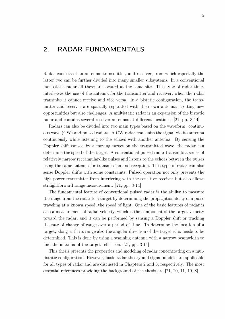
Mixer and frequency translation are discussed in more detail in Section 3.3 anddetection in Section 3.4. Filters along with noise and how they interact are explainedin Section 3.5. These topics are related to the simulation tool introduced in Chapter4. There are other important components in radar as well but the details are beyondthe scope of this thesis. Some practical aspects of components in modeling arediscussed in Section 4.2.
Radar generates a baseband pulse train with a desired pulse length and PRF

3. Radar Modeling 26
in a waveform generator. The baseband signal is raised to radio frequencies, andit is done in several phases. The first mixer after waveform generator in Figure3.1 raises the baseband pulses to an intermediate frequency (IF) fif. IF-signal isthen band-pass filtered and amplified. Filtering is needed to remove the unwantedcomponents and to increase the SNR. The second mixer further moves the pulses upto the carrier frequency fc ready to be transmitted via the antenna. Modulating acontinuous wave signal with rectangular pulses in a mixer results in similar waveformas in the example of Figure 2.1 except one pulse can contain hundreds or thousandsof sine wave periods.
For the sake of clarity only one IF stage is presented in Figure 3.1 but in practicalradars there may be more to make frequency translation and filtering of imagefrequencies easier. Despite the number of stages, the principle of operation remainsthe same; the intermediate frequency stays constant while the frequency synthesizeroutput fc − fif is changed if the carrier frequency fc needs to be varied. This makesthe design and implementation of the IF stage and IF-filters simpler.
On reception the captured RF signal is down-converted with a mixer from fc tofif. After filtering and amplifying the signal is detected in a synchronous detectordiscussed in more detail in Section 3.4. However, detector has two outputs: theIn-phase (I) signal and the Quadrature-phase (Q) signal. Both the amplitude andphase information of the received signal can be extracted from these signals. Theseoutput signals are baseband signals corresponding to the waveform generator outputon the transmitter side. The signals are low-pass filtered (anti-aliasing filter) andconverted to digital signals for processing. A trend is to move the AD-convertercloser to the antenna, for example, to the IF-stage when it is possible. This setshigh requirements for the converter but the benefits of digital operation is achievedin the larger part of the receiver.
A low frequency stable local oscillator (LO) generates a continuous sine wavewhich is as immune as possible to the variations of environmental variables such astemperature, humidity, aging, and supply voltage. All the other frequencies in theradar are locked in and derived from the local oscillator. The upconverter creates afixed IF and the frequency synthesizer generates the needed frequency (fc − fif) tocreate the desired carrier frequency (fc). The simulation model presented in Chapter4 follows this general block diagram introduced here.
3.2 Basic Signal Model
Before explaining the components of the block diagram in more detail, an illustrativeway to represent radar signals is introduced. Continuous sine wave signal
a(t) = A cos (ωt+ ϕ) (3.1)

3. Radar Modeling 27
−2 −1.5 −1 −0.5 0 0.5 1 1.5 2
x 106
0
0.2
0.4
0.6
0.8
1
Frequency / Hz
Figure 3.2: Frequency domain representation of a sine wave with f0 = 1 MHz.
has frequency domain representation in Figure 3.2. Real sine signal has a reflectedspectrum with respect to the zero frequency so the frequency components are f0
and −f0. One explanation for the negative frequency can be ratified in the phasorrepresentation which is also used in literature [21, 10] to illustrate signals. Thephasor representation of complex signal
A(t) = Aej(ωt+ϕ) (3.2)
can be seen in Figure 3.3a. Phasor lies on the complex plane, has a length of A,rotates counterclockwise about the origin with an angular velocity of ω, and hasan initial phase angle of ϕ. Phasor representations are used in [21] and [10] toillustratively present signals, noise, modulations, and Doppler shift.
The instant value of the Signal (3.2) can be considered as a frozen phasor butalso a complex number or a vector on the complex plane. In general, when realor complex number is multiplied by ejϕ the corresponding vector or phasor rotatescounterclockwise on the complex plane by angle ϕ without affecting its length (ab-solute value). When a continuously increasing angle ωt is added, the phasor rotates.
Cosine signal is the projection of the rotating phasor on the real- or x-axis, seenin Figure 3.3a. By the trigonometric identities, cosine, or the real-axis projection,signal can be presented as
cos (ωt+ ϕ) = Re(ej(ωt+ϕ)
)= cos (ωt+ ϕ) =
1
2
(ej(ωt+ϕ) + e-j(ωt+ϕ)
). (3.3)
The sum of these two exponential functions, or rotating phasors, is always on the realaxis. Thus real signal can be presented as two phasors rotating opposite directions,seen in Figure 3.3b. These phasors have opposite frequencies and in the spectrumof the real signal are two opposite frequency components. Similarly sine functioncan be represented by two exponential functions.

3. Radar Modeling 28
(a) Complex signal has one rotating phasor.Projection of rotating phasor on the real andimaginary axes are the cosine and sine func-tions, respectively.
(b) Real cosine signal can be represented withtwo phasors rotating opposite directions result-ing in the projection on the real axis.
Figure 3.3: Phasor representations of complex and real signals.
Stimson [21] describes phasor diagram as a rotating phasor illuminated by astrobe light, hence resulting in a static figure when the strobe frequency equals therotating frequency. If the reference, or the strobe light, stays constant while thesignal encounters phase shift, the phasor starts to rotate in the following diagramsof frozen instants. The phenomenon has an analogy to the received radar signal andDoppler shift.
The signal reception of radar is a multi-stage system but the aforementionedsituation can be considered between the synchronous detector and AD-converter inFigure 3.1. I- and Q-signals combined is a complex signal which can be representedas phasor. The receiver of pulsed radar takes a sample of the pulse and a phasordiagram can be considered as one complex IQ-sample. Sampling frequency equalsfPRF and corresponds the strobe light mentioned above. If target is stationary,consecutive phasor diagrams are the same. When the target moves, carrier waveencounters Doppler shift and phasor starts to rotate on the consecutive samplinginstants.
Between two sampling instants, or pulses, phasor rotates a certain angle whichover time forms certain frequency. The maximum frequency is achieved when thephasor rotates half revolution, or π, in a sampling period 1/fPRF s. This frequencyis half of the sampling frequency, or the Nyquist frequency, fPRF/2. If the changeof phase between samples is larger, the interpretation becomes ambiguous since itcannot be determined if the phasor actually rotated to that point from the other

3. Radar Modeling 29
direction, thus the absolute value getting smaller but the sign reversed. Similarly itcannot be known if the phasor rotates many full revolutions between the samples. Ifdifference is 2π, the frequency is 0 Hz. This is one more interpretation for the sam-pling theorem and aliasing. The ambiguous frequency range is −fPRF/2...fPRF/2.
3.3 Mixer Frequency Translation
Frequency mixer is an important component in radars and other radio frequencydevices. Mixer creates new frequencies from the frequencies fed to it and in radiotransmitters and receivers it is used to shift signals from one center frequency to an-other. The important property of mixer is that the signal bandwidth and modulationremain intact in frequency shifting, or frequency translation. Frequency translationis needed since some operations can be only performed in low or high frequencies,or at constant frequency range. One such an operation is filtering where the ratioof the bandwidth and center frequency strongly affects the filter implementation.Changing the center frequency while the bandwidth stays intact allows varying thisratio. If this center frequency is kept constant by changing the frequency translation,the implementation of the filter is easier and the result better. This is also donein radar as was presented in the block diagram in Figure 3.1; IF is constant evenif the transmitting frequency is varied. On the other hand, transmitted frequenciesare determined by the type and requirements of the radar, the size of the antenna,government regulations, atmospheric attenuations, and other external reasons. Byusing frequency translation these does not have to affect the inner structure of thetransmitter and receiver. Description of mixers in more detail can be found in [10,pp. 261-343].
If two signals with frequencies f1 and f2 are fed into a mixer which is a nonlineardevice, the output frequencies are the harmonic and intermodulation components ofthese frequencies,
fout = |nf1 ±mf2| , (3.4)
where n and m are integers 0, 1, 2, ... and n + m the order of the response. Thehigher the order the smaller the output power, so the second order response is usedin mixers so the desired output is f1±f2. The unwanted components are filtered out,and the conversion scheme is designed so that none of the unwanted components aretoo close to the signals of interest. [10, pp. 264-265].
Since the sum and difference frequencies are used and other components filteredout, this can be used as an approximation of the mixer operation and is also usedat this point in the simulation tool presented in Chapter 4. The generation of thesum and difference frequencies from two frequency components is the result of themultiplication of the signals in the time domain or the amplitude modulation. If

3. Radar Modeling 30
the information signal with amplitude information Am(t) and phase or frequencyinformation ϕm(t)
sm(t) = Am(t) cos (ωmt+ ϕm(t)) (3.5)
is multiplied with the carrier signal (with amplitude of 1)
sc(t) = cos (ωct) (3.6)
the result is
sm(t)sc(t) = Am(t) cos (ωmt+ ϕm(t)) cos (ωct) (3.7)
=Am(t)
2cos [(ωc + ωm)t+ ϕm(t)] +
Am(t)
2cos [(ωc − ωm)t− ϕm(t)]
using the known trigonometric identity cos(α) cos(β) = 12cos(α+ β) + 1
2cos(α− β).
Equation (3.7) shows that the level of generated components drops but also thatpossible amplitude and phase modulations pass the multiplication. [10, pp. 264-267]
The time domain multiplication of two signals is similar to amplitude modulation.If the amplitude of the carrier wave is modulated by the information signal,
sAM(t) = [1 + sm(t)] sc(t) (3.8)
= [1 + Am(t) cos (ωmt+ ϕm(t))] cos (ωct)
= cos (ωct) +Am
2cos [(ωc + ωm)t+ ϕm(t)] +
Am
2cos [(ωc − ωm)t− ϕm(t)].
Now also the carrier signal is present at the output which is true in many situations.The maximum amplitude Am, or in general Am divided by the carrier amplitude,is the modulation index µ which describes the depth of the modulation, usually inpercents. [10, pp. 105-107]
Considering the receiver mixer 3 in Figure 3.1 the RF-signal captured by theantenna is filtered and amplified with a low-noise amplifier (LNA) and then fed toa mixer. This real signal of the frequency fc can be expressed as
cos(ωct) =1
2
(ejωct + e−jωct
)(3.9)
as was presented in Section 3.2. The second signal fed to the mixer is the frequencysynthesizer signal of the frequency fc − fif:
cos ((ωc − ωif)t) =1
2
(ej(ωc−ωif)t + e-j(ωc−ωif)t
). (3.10)

3. Radar Modeling 31
Using the multiplication approximation for the mixer the output is
cos(ωct) cos ((ωc − ωif)t) =1
2
(ejωct + e-jωct
) 12
(ej(ωc−ωif)t + e-j(ωc−ωif)t
)(3.11)
=1
4
(ej(2ωc−ωif)t + e-j(2ωc−ωif)t + ejωift + e-jωift
)=
1
2cos ((2ωc − ωif)t) +
1
2cos(ωift).
This sum signal is filtered with a band-pass filter, the bandwidth centered at IF, sothat 2fc − fif component is filtered out. Similar analysis can be done on the trans-mitter side of the presented block diagram in Figure 3.1. However, when shiftingthe signal higher on the frequency band the lower component is filtered out.
3.4 Synchronous Detector
Detector shifts a signal from the IF further down and has an operation similar to amixer. However, detector translates the signal all the way to the baseband ready forAD-converter to digitize it before processing. Detector signals can be examined thesame way as mixer signals when performing a frequency translation from RF to IFas in Section 3.3. As is presented in Figure 3.1, the dashed line information signalfrom IF-filter and -amplifier block and the reference signal from Upconverter bothhave a frequency of fc. As detector has a similar operation to mixer, also resultingin sum and difference frequencies, obviously the difference component is centered atzero hertz and is a baseband signal.
Similarly as with the mixer, now also including the phase of the signal, two signalsare present: the information signal
cos(ωift+ ϕif) (3.12)
is multiplied with the IF reference from the upconverter
cos(ωift), (3.13)
hence resulting in
cos(ωift+ ϕif) cos(ωift) =1
2
(ej(ωift+ϕif) + e-j(ωif+ϕif)
) 12
(ejωift + e-jωift
)(3.14)
=1
4
(ej(2ωift+ϕif) + e-j(2ωift+ϕif) + ejϕif + e-jϕif
)=
1
2cos(2ωift+ ϕif) +
1
2cosϕif.
After low-pass filtering only the constant phase-dependent component remains. In
3. Radar Modeling 32
Figure 3.4: Synchronous detector block diagram. IF signal is the input to synchronousdetector in Figure 3.1.
general, as was discussed in Section 2.3 and presented with Equation (2.9), the phasedifference between the transmitted and the received wave depends on the range ofthe target. When the result of Equation (3.14) is combined with Equation (2.9),the signal magnitude after detector, also considering low-pass filter and mergingamplitude 1
2to the A, is
Ad = cos
(−2π
2R
λc
). (3.15)
As the wavelength λc is fixed, the magnitude of the received signal after the detectordepends on the range of the target. Thus, even a constant-RCS moving targetgenerates a varying magnitude signal, the phenomenon not to be confused withRCS fluctuation or scintillation. Furthermore, targets can lie in blind spots wherethe amplitude goes to zero.
To prevent the magnitude variation due to range, and to make Doppler processingpossible, modern radar with a synchronous detector, also called IQ-demodulator orcoherent detector, uses I and Q channels to detect the signal phase and amplitude.It performs a frequency conversion and generates a complex signal I+jQ centeredat zero frequency. To achieve that a phase delayed version of the IF reference isused together with the original reference. An illustration of a synchronous detectoris presented in Figure 3.4. [20]
The IF reference is split into two signals with the phase difference of 90◦, or π/2.The convention is to have the Q lagging the I by 90◦. Depending on the configurationdifferent signs for the phase difference of the IF references need to be used to achievethe desired output where Q lags I. Hence in the example here the second reference

3. Radar Modeling 33
leads by 90◦. The leading reference
cos(ωift+
π
2
)= − sin(ωift) (3.16)
is multiplied with the Signal (3.12):
cos(ωift+ ϕif) (− sin(ωift)) =1
2
(ej(ωift+ϕif) + e-j(ωif+ϕif)
) 1
j2(−ejωift + e-jωift
)(3.17)
=1
j4(−ej(2ωift+ϕif) + e-j(2ωift+ϕif) + ejϕif − e-jϕif
)= −1
2sin(2ωift+ ϕif) +
1
2sinϕif
which is the Q signal and the result of Equation (3.14) is the I signal. These arelow-pass filtered, amplified by two, and combined to get the synchronous detectoroutput
I + jQ = cosϕif + j sinϕif = ejϕif (3.18)
which is the complex phasor discussed in Section 3.2. This signal is also a function ofthe phase ϕif and thus a function of the range of the target. However, the range doesnot affect the amplitude of the signal but the phase of it which is the needed result forthe Doppler processing. The result given here is a counter-clockwise rotating phasorwhen the target is approaching resulting in a positive Doppler frequency which isa convention in radar theory. Depending on the frequency conversion schemes, thesign of the phase difference of the IF-reference, or the sign of the I or Q sample inthe processing stage, may need to be changed to achieve the mentioned convention.Here the sign of the IF-reference was changed. [20, pp. 6.31-6.35]
After discussing about the IQ-detected and range-independent amplitude it shouldbe noticed that in practice the amplitude scintillates because of the changing RCSwhich is a significant phenomenon with practical targets. However, by preservingthe phase information the radar can perform an efficient integration of several pulsesover a certain period of time by Doppler processing as was described in Section 2.4.
3.5 Noise Filters
Filters are used to pass wanted signals or remove unwanted signals, or in generalto change the amplitude and phase of certain frequencies. Filters can be analog ordigital both having their own advantages and disadvantages as well as limitations.Filters at the highest frequencies are analog since these signals cannot be convertedto digital. Digital filters are commonly used where it is possible because they oftenoffer better performance and do not significantly suffer from varying environmentalvariables such as temperature, humidity, aging and mechanical disturbances. Dig-
3. Radar Modeling 34
ital filters can be also steeper and more selective than their analog counterparts.Some filter theory and analog filters are discussed in [10, pp. 143-260] and in manyelectronics books, and digital filters as well as comprehensive filtering theory in thetime and frequency domains in [3].
Filters are used in radar between different parts to remove unwanted signalssuch the image frequencies and unwanted mixer output components. Filters fromRF until anti-aliasing filter of the AD-converter are analog and after that digital.Besides removing unwanted signals, another task of filter is to remove noise outsidethe bandwidth of the signal of interest. Filters are considered here from this pointof view and noise introduced since it is an important part of the simulation toolpresented in Chapter 4. Other filter characteristics can be found on the booksmentioned above.
Noise can be characterized by its frequency and amplitude distributions. Themost common type of noise is the white Gaussian noise (WGN) referring to the flatfrequency spectrum and Gaussian-shaped amplitude distribution usually with zeromean value. Other frequency distributions, or colors, are 1/f noise which is oftencalled pink or flicker noise and 1/f 2 noise called red or brownian noise. The spectrumcan also be more complex as often is the phase noise in oscillators. An example ofa different amplitude distribution is the quantization noise of an analog-to-digitalconverter which has a uniform distribution.
Noise need to be examined in a limited bandwidth because otherwise the powerwould be infinite due to the infinite frequency spectrum. Since white noise has aconstant power spectrum, the power is directly proportional to the bandwidth. Thuswhite noise is a theoretical concept and in practice it is always bandwidth-limited,nevertheless called white noise. In practice the bandwidth is always limited by somephysical constraints. Two examples of sine signals with additive white Gaussiannoise with different noise bandwidths are presented in Figure 3.5. The noise powerspectral density (Watts / Hz) is the same in both signals. The signal in Figures3.5a and 3.5b has a noise bandwidth of 500 MHz and SNR of 7 dB. By limiting thebandwidth to one tenth, 50 MHz, the SNR is raised 10 dB to 17 dB, seen in Figure3.5c and 3.5d. Despite the equal noise power density the former one has higheroverall noise power due to the larger bandwidth.
In analog systems the noise bandwidth is infinite in theory and in practice limitedby parasitic impedances. However, in digital systems the sampling frequency limitsthe noise bandwidth to some known and reasonable value since no frequencies higherthan the Nyquist’s frequency can exist in the signal. The signal can be furtherfiltered inside the system to further limit the bandwidth. In the example above thesine wave stays intact when lowering the bandwidth. Therefore, the signal powerremains constant and SNR is improved by the factor the noise power is reduced.

3. Radar Modeling 35
0 0.5 1 1.5 2 2.5 3
x 10−6
−2
−1.5
−1
−0.5
0
0.5
1
1.5
2
Time [s]
(a) Time domain, 500 MHz BW, SNR =7 dB.
−2.5 −2 −1.5 −1 −0.5 0 0.5 1 1.5 2 2.5
x 108
0
0.05
0.1
0.15
0.2
0.25
0.3
0.35
0.4
0.45
0.5
Frequency [Hz]
(b) Frequency domain, 500 MHz BW,SNR = 7 dB.
0 0.5 1 1.5 2 2.5 3
x 10−6
−1.5
−1
−0.5
0
0.5
1
1.5
Time [s]
(c) Time domain, 50 MHz BW, SNR =17 dB.
−2.5 −2 −1.5 −1 −0.5 0 0.5 1 1.5 2 2.5
x 108
0
0.05
0.1
0.15
0.2
0.25
0.3
0.35
0.4
0.45
0.5
Frequency [Hz]
(d) Frequency domain, 50 MHz BW,SNR = 17 dB.
Figure 3.5: 1 MHz sine wave with two different noise bandwidths. In spectra the twosignal spectrum spikes are close to each other and appear as one thick spike. In Figuresa-b noise bandwidth is 500 MHz resulting in SNR of 7 dB with the added noise spectraldensity. In Figures c and d the bandwidth has been reduced to 50 MHz resulting in SNR of17 dB.
When more complex signal is used, at some point some signal power starts to filterout as well. The optimal filter to maximize SNR is called a matched filter and it isgenerally used in communications engineering. Mathematically the impulse responseof the ideal matched filter is the time-reversed complex-conjugate of the signal tobe filtered.
3.6 Oscillator
Oscillator and timing circuits play crucial role in radar. Typically first local oscil-lator needs to be stable low frequency oscillator, which is as immune as possible tothe variations of environmental variables, is used and other oscillator and timingcircuits, and frequency synthesizers are locked in and derived from this oscillator.Stable phase-coherent operation is needed for the Doppler sensing and processingand accurate timing for range measurement. Stable digital clock signals are needed

3. Radar Modeling 36
(a) Noise is a statistical phenomenon soits RMS value can be presented in circles ofpropabilities.
(b) Noise can be split into amplitude (AM)and phase (PM) components.
Figure 3.6: Noisy reference sine signal is the sum of the ideal signal and noise.
for processing and especially AD-converter. [20, pp. 6.14-6.18]In theory oscillator output would be pure sine wave but in reality it contains
interferences and instabilities which can be characterized both in the time and fre-quency domains. A model for oscillator signal can be generated similarly than inearlier sections. Oscillator output voltage
V (t) = [V0 + ϵ(t)] sin [2πf0 + ϕ(t)] (3.19)
where V0 and f0 are the nominal amplitude and frequency, respectively, and ϵ(t) isthe amplitude noise, and ϕ(t) the phase noise. These noise components in phasorsignal are shown in Figure 3.6 where AM (Amplitude Modulation) represents ϵ(t)
and PM (Phase Modulation) ϕ(t). This separation of noise into components israther theoretical but they can have different frequency characteristics. In high-performance sources amplitude noise, or ϵ(t) in Equation (3.19), is usually negligibleand phase noise is of interest. It can be also noticed that these components affectunequally the signal when considering the real signal as the projection on the realaxis. For example, in zero crossings AM has no effect but PM causes uncertainty tothe zero crossing instant. In digital clock signals this is often called clock jitter, andfor example in AD-converter it causes noise and distortion because of the variationof sampling instances. Figure 3.6a shows the circles of noise values where they canrepresent for example σ, 2σ, and 3σ values if the statistics are Gaussian. If the realand imaginary components of the noise are independent and Gaussian distributed,the length of the noise phasor, or the magnitude, is Rayleigh distributed and thephase angle uniformly distributed [10, pp. 102-103]. [17], [10, pp. 345-360]
Oscillator interferences have effect on the radar performance. It is assumed that

3. Radar Modeling 37
the propagation path of synchronization signal can cause or increase similar effectsas in oscillators introduced here and in [10, pp. 345-360], [17], and [20, pp. 6.14-6.18]. Thus, the noise separated into AM and PM components as well as amplitudeand frequency modulations for slower effects are modeled in the simulation tool asreference signal errors.
Bistatic and multistatic radars need two different synchronizations: time andphase synchronization. Time synchronization is needed to adjust the timing of thereception for range measurement. Timing accuracy is typically on the order of afraction of the pulse length. The synchronization can be implemented for exam-ple using the transmitted signal from the transmitter via land line, communicationlink or direct signal propagation if line of sight exists between transmitter and re-ceiver. Periodically synchronized stable clocks on transmitter and receiver sites canbe also used. If direct propagation path or external link is used, the propagationerrors dominate and need to be carefully considered. Phase synchronization be-tween transmitter reference and receiver reference with much higher requirementsis needed for phase-coherent operation for Doppler processing. Synchronization canbe implemented by locking the receiver to the transmitter or by periodically updat-ing accurate clocks. However, the accuracy requirements are higher than in timesynchronization and depend on the needed phase accuracy. This can be from lessthan one degree to tens of degrees of phase meaning many decades higher accuracythan in time synchronization. One major difference between monostatic and mul-tistatic radar is that low-frequency effects cancel out in monostatic radar becausethe variations are insignificant during the pulse propagation time while in bistaticor multistatic radar these errors may be additive instead [28]. Also in the simula-tion time-consuming imaging methods wanted to be used and therefore the possiblecoherent time for the reference is much longer. [23, pp. 258-259]

38
4. SIMULATION ENVIRONMENT
A simulation tool has been developed to allow examining the operation of radar. Thestructure of the simulation model follows the general construction of pulsed Dopplerradar which was discussed in Chapter 3 and illustrated in Figure 3.1. However, focushas been in the simulation of multistatic radar so modeling the timing and phasecoherence has been the main aspects in developing the simulation model. Since thesimulation tool has a modular structure, it is easy to adjust the model to meet variousneeds or to enhance the model by adding more features into it and making it moreaccurate. The tool has been created using MATLAB/Simulink software. The systemconsists of the signal generation, transmission, reception, reference transmission, andthe target model, and it is created by using generic Simulink blocks and embeddedMATLAB code. Initializations and the processing of the output data are executedwith conventional MATLAB scripts and functions and graphical user interface isunder development. Despite the reference interferences which are the main aspectof the model, ideal models of components have been used. Some ideas to modify theideal models to represent practical components better are presented in Section 4.2
Radar configuration in simulation is bistatic radar with transferred reference sig-nals which can model fiber optics or other direct transmission of references. Thissetup was chosen because of specific interest in one real experimental radar. Wave-form options are versatile and carrier frequency, PRF, and pulse width can be chosen,and also the carrier can be varied in sequences. The stepped-frequency waveform canbe used to achieve high range resolution. The group of pulses running throughoutthe bandwidth of the waveform from the lowest to the highest frequency is calledburst. Similarly as PRF there is a burst rate which is much lower than the PRF, forexample in case of 128 pulses 128 times lower. One of the purpose of the simulationis to offer a possibility to experiment what are the stability requirements for thereference signals in the burst repetition interval which can be significantly longerthan pulse repetition interval, and how the end signal is affected if the reference isnot within the accuracy limits. Thus, as the point of the simulation is to modelreferences with interferences it is made easily possible.
Simulink simulation is executed by calculating the system variables and statesat discrete time steps, simulation steps, which are the fundamental time units ofthe simulation. That also represents the fundamental sampling frequency of the

4. Simulation Environment 39
Figure 4.1: Top level block diagram.
system limiting the frequencies that can be expressed without aliasing, consideringNyquist-Shannon sampling theorem [18, 13]. Simulink offers a possibility to modelcontinuous time system by internally simulating continuous time system by dividingsimulation steps into smaller substeps and solving the state of the system morefrequently. Simulation step can be chosen to be fixed or variable, the latter varyingbased on the derivatives of the signals in simulation. However, to have the mostcontrolled awareness of the operation of the simulation, discrete time operation andfixed simulation step have been chosen. The changes on the initialization of thesimulation are done in matlab script.
4.1 Introduction of Simulation Tool
The top level block diagram of the simulator is in Figure 4.1 and block functionsare explained in more detail in the following sections. Important signals in top levelblock diagram are shown in Table 4.1. The simulation model presented here is abistatic configuration containing one receiver so multistatic response needs to besimulated in several phases. Signal generator block corresponds a radar transmit-ter generating all the necessary signals needed for signal transmission and coherentreception. The IF-reference and the variable reference go through the propagationdelay which produces a fixed propagation delay for references. This represents thedelay due to the transmission of the references between different sites in bistatic ormultistatic configuration. The variable reference also goes through the interferenceand noise block where errors can be added to the signal to model the propagationpath. Hence, in the example simulation configuration presented interferences areadded only to this reference while keeping IF-reference clean. An embedded MAT-LAB function signalDelay represents a propagation delay for the transmitted radiowave signal, as well as a target model by calculating the superposition of the reflectedsignals from multiple point scatterers forming a target. Downmix and IQ-detectorblocks form the receiver, consisting of mixers, filters, and the detector. GeneratedIQ-samples are then stored for processing in MATLAB.

4. Simulation Environment 40
Table 4.1: Top level block diagram signals.
Signal PurposeSignal generatorif ref r Intermediate frequency reference (real sine signal)var ref c Variable frequency reference (complex sine signal)sig trig Generates rising edge in the beginning of a pulsesig phase Continuous phase signal (range −π...π)clock Running simulation time (in seconds)Downmixref in r Variable reference signal input (real)sig in r RF-signal input (real)out r Output at IF (real)IQ-detectorref in r IF-reference signal input (real)sig in r IF-signal input (real)out c I and Q outputs combined as a complex signal
Signal Generation
Signal generation is actually performed in two blocks. The Signal generator blockgenerates reference, or synchronization, signals for coherent reception and controlsignals for pulse generation which is located in Propagation and target model blockdue to practical reasons explained in Section 4.1. The block diagram of the signalgenerator is presented in Figure 4.2 and signals and blocks in Table 4.2. The blockoutputs from top downwards are: simulation time (clock), real IF reference (if refr), complex variable reference (var ref c), RF signal phase (sig phase), and pulsetrigger (sig trig). RF-pulse is generated outside the signal generator in Propagationand target model using the latter two signals.
All signals are derived from the fundamental frequency ,which determines thefrequency resolution of the signals generated, and are integer multiples of the funda-mental clock frequency. This corresponds stable low frequency local oscillator andfrequency synthesizers in radar although phase-locked loops or synthesizers have notbeen modeled. Signals are derived using complex sine waves and exponential func-tions together acting as an ideal mathematical phase-lock. This maintains the samephase relative to the fundamental clock signal in every pulse burst when changingthe carrier frequency. Without the preservation of the phase relations, meaningall the frequencies in a stepped frequency waveform remaining coherent, a differentphase at every pulse burst would be generated destroying the construction of thedown range in inverse Fourier transform.
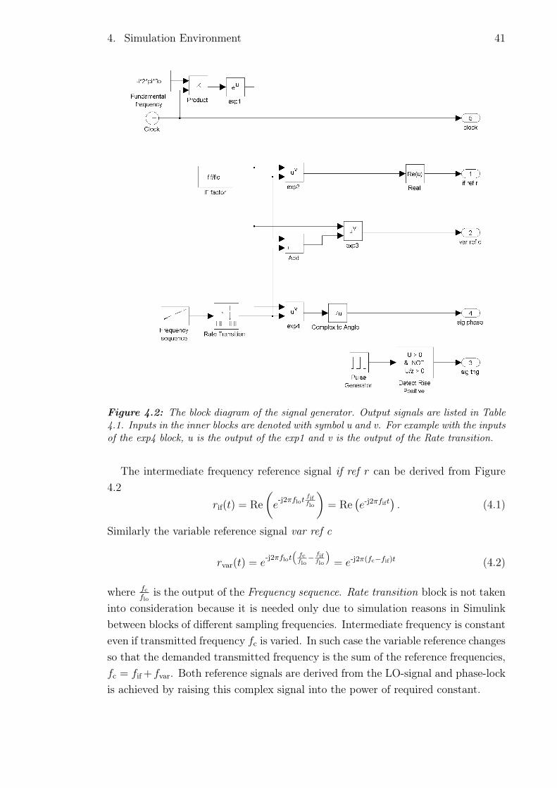
4. Simulation Environment 41
Figure 4.2: The block diagram of the signal generator. Output signals are listed in Table4.1. Inputs in the inner blocks are denoted with symbol u and v. For example with the inputsof the exp4 block, u is the output of the exp1 and v is the output of the Rate transition.
The intermediate frequency reference signal if ref r can be derived from Figure4.2
rif(t) = Re(e-j2πflot
fifflo
)= Re
(e-j2πfift
). (4.1)
Similarly the variable reference signal var ref c
rvar(t) = e-j2πflot
(fcflo
− fifflo
)= e-j2π(fc−fif)t (4.2)
where fcflo
is the output of the Frequency sequence. Rate transition block is not takeninto consideration because it is needed only due to simulation reasons in Simulinkbetween blocks of different sampling frequencies. Intermediate frequency is constanteven if transmitted frequency fc is varied. In such case the variable reference changesso that the demanded transmitted frequency is the sum of the reference frequencies,fc = fif + fvar. Both reference signals are derived from the LO-signal and phase-lockis achieved by raising this complex signal into the power of required constant.

4. Simulation Environment 42
Table 4.2: Top level block diagram signals.
Constant Purposeflo Frequency of local oscillatorfif Intermediate frequencyBlock PurposeFundamental frequency Together with Product and exp1 generates
the local oscillator signal e−i2πflo
Clock Running simulation time (in seconds)IF factor Integer fIF/flo, used to multiply flo to gener-
ate fIF
Frequency sequence Generates the factor to multiply flo to gen-erate desired fc. Factor changes after PRI ifmultiple values of fc are used, thus generat-ing a sequence.
Rate transition Inner Simulink block needed between twoblock with different sampling frequency.
Pulse generator Generates pulse train based on given PRFand pulse width values.
Detect rise positive Output is high on the rising edge of the inputand otherwise low.
Radio wave signal to be transmitted is not generated in the signal generatorbecause of simulation time step considerations explained in 4.1. Instead, controlsignals for generating the pulse train are generated. Instant phase output
ϕs(t) = Arg(e-j2πflot
fcflo
)= Arg
(e-j2πfct
), (4.3)
bounded between −π and π, of sig phase and trigger of the rising edge of the pulsesig trig along with the clock are used in the embedded code block Propagation andtarget model block to generate the RF-pulses.
Reference Signal Transmission
Complex variable reference signal var ref c is fed into the Interference and noiseblock, seen in Figure 4.3, where noise and interferences can be added to the signalto model the propagation path. In the simulation presented, interferences are onlyadded to this variable reference signal but only to make the amount of variablessmaller. The block can be just copied to the propagation path of the if ref r as wellif needed. The Interference and noise block can generate gaussian and uniformlydistributed amplitude and phase noise, and frequency and amplitude modulations.The blocks illustrated in Figures 4.4a and 4.4b perform the noise generation and

4. Simulation Environment 43
Figure 4.3: The block diagram of the interference and noise block.
(a) Amplitude noise. (b) Phase noise.
Figure 4.4: Generation of noise inside the interference and noise block. The noise canbe shaped to a specific type by using filters in the noise path.
Figure 4.5 presents the model for frequency modulation. Amplitude modulation isgenerated by using a plain sine wave generator seen in Figure 4.3.
The input is a complex signal to allow the addition of theoretical phase noise.Correspondingly, amplitude noise only affects the magnitude of the complex signal.In practice, the amplitude and phase components of the noise may be inseparablebecause the signal in which they emerge is real as is also the output signal of theInterference and noise block. However, the model discussed here enables the com-ponents to have different characteristics. Phase noise often has a specific spectrumshape, especially true for oscillators where amplitude noise can be insignificant,therefore an accurate model can be created by using filters in the phase noise path.
The implementation of the Frequency modulation block can be seen in Figure 4.5generating a signal
ϕFM(t) = µFM sin (ωFMt) (4.4)
Figure 4.5: Frequency modulation in the interference and noise block.

4. Simulation Environment 44
where µFM is the modulation index and ωFM the modulation frequency. Signal(4.4) represents a varying phase signal which is added to the phase noise ϕn(t) inInterference and noise, resulting in
pn(t) = e-j(ϕn(t)+µFM sin (ωFMt)) (4.5)
before Add pnoise block in Figure 4.3. This is multiplied with the input signal whichis the signal (4.2). Substituting ωvar = 2π(fc − fif) for simplicity
p(t) = e-jωvarte-j(ϕn(t)+µFM sin (ωFMt)) = e-j(ωvart+ϕn(t)+µFM sin (ωFMt)). (4.6)
Amplitude noise an(t) with mean value of 1 is added to the signal and the realpart of the result is taken. Finally amplitude modulation of frequency ωAM andmodulation index µAM can be added with the sine generator. Thus, the output outr of the Interference and noise can be written as
s(t) = [1 + µAM sin (ωAM)]Re[an(t)e
-j(ωvart+ϕn(t)+µFM sin (ωFMt))]. (4.7)
Certainly, if error and interference sources are set as zero the Interference and noiseblock passes the input signal directly without any distortions.
Target Model
Target model is realized using embedded MATLAB function block containing codeoptimized for Simulink use. For the sake of efficiency, these functions are compiledbefore executing so there are constraints on the code to make compiling possible.High efficiency is needed since the function is executed on every simulation step.
A target for a simulation is created using a group of point scatterers. Each pointhas a specific location in space and RCS value. By using sufficient amount of points,more complex targets can be created. The simulation calculates the reflectionscaused by individual scatterers and sums them to form the superposition response.The location of the particle causes corresponding delay. The modeling of the targetitself, the group of points, is not a topic here so the simulation tool operates withpre-processed matrices which contain the location and RCS of point scatterers in afunction of time, in fact in a function of discrete PRI steps. The task to make pointsmoving is not difficult but how RCS changes requires more consideration.
Since computer simulation is always a discrete process and the time delay accu-racy for proper phase reconstruction is rather high, the implementation needs somespecial attention. Simulation is executed by calculating the system variables andstates at discrete time steps, simulation steps, which are the fundamental time unitsof the simulation. Since these are the smallest possible time unit in the simula-

4. Simulation Environment 45
Figure 4.6: Circles represent the sampling instants of the signal. Signal in the middle isthe uppermost delayed by one sample. The undermost signal is the uppermost delayed byhalf a sample, implemented by resampling the signal.
tion model, it arouses some constraints. When delaying the transmitted signal inPropagation and target model block, based on the length of the propagation pathof the pulse train, the smallest possible discretization step of the delay equals thesimulation step. Because the fundamental sampling frequency, the reciprocal of thesimulation step, is 5-10 times the highest frequency in the system, one simulationstep equals tens of degrees in the radio frequency signal phase. In a simulation whereinterferences causing one degree error are to be examined, the delay adjustment inthat way is too coarse.
To overcome this problem the signal can be resampled and the sampling pointscan be chosen so that the required delay is an integer multiple of the simulationstep. An example can be seen in Figure 4.6. However, resampling is too slowprocess to do accurately at every simulation step. In a simulation environment,with some assumptions, the problem can be solved by generating the signal usingthe convenient sampling instant in the delaying point of view. Since the neededdelay is known and the initial phase of the generated signal can be obtained fromthe Signal generator block, the signal can be generated so that the needed delay isan integer multiple of the simulation step. So, after all, the delay in total consists ofan integer multiple of the simulation step as a coarse delay adjustment and the phaseshift which is the fine adjustment of the delay. This method allows for very accurate

4. Simulation Environment 46
Figure 4.7: The block diagram of the downmix from radio frequency to intermediatefrequency.
setting of the delay. As a summary, instead of delaying the signal it is actuallycreated when the needed delay has already passed, using the delay and initial phaseinformation. As a result, when using sine wave signal, the target model outputsignal corresponds exactly a delayed version of the transmitted signal. This can alsocause limitations, for example, if oscillator errors, which affect both transmitted andreference signals, are to be modeled in the future.
Downmixing and Detection
The first stage of the signal reception is the downmixing of the RF pulse traininto the intermediate frequency (IF). This is done using a mixer, as can be seen inFigure 4.7. Mixer produces sum and difference components of the frequencies fedto it. Since on reception the signal needs to be downmixed the higher componentis filtered out. Thus a band-pass filter centered at IF follows the mixer. The filterbandwidth must be wide enough to pass the signal without significant attenuationbut narrow enough to considerably attenuate the image frequencies and excessivenoise. The gain stage compensates the loss of power when filtering out the imagefrequencies. Filter type on Simulink is discrete filter due to the fact that signals arediscrete digital signals sampled at every simulation step.
The received signal is detected to baseband frequencies using 2-channel IQ-detector, see block diagram in Figure 4.8. The downmixed IF-signal is mixed withthe IF-reference and the 90◦ delayed version of the IF-reference to generate base-band I and Q signals. I and Q samples are combined to form one complex sample.The complex signal is then fed to a low-pass filter to filter out the higher imagefrequencies and amplified to compensate the power loss.
In detector signal needs to be delayed exactly 90◦, so similar problem arises as indelaying the pulse, explained in Section 4.1. Here resampling is not even acceptablemean since it would modify the signal while it should be an identical delayed copy ofthe reference used for the I-channel detection. However, the delay is always constantin phase and also in time because IF is constant even if the carrier frequency ischanged. Hence, in fact the simulation step for the whole simulation is chosen sothat the 90◦ in IF is an integer multiple of the simulation step. This can be donebecause there is nothing that requires some exact time for the simulation step. In

4. Simulation Environment 47
Figure 4.8: The block diagram of the IQ-detector.
the test simulation and in Figure 4.8 the delay is 2 simulation steps.
4.2 Non-Ideal Models
Despite the promising platform for real-life imitating simulations is achieved, con-siderable amount of work is still needed to get reliable results since most parts inthe simulation are modeled as ideal components using only mathematical formulae.Models need to be modified to contain at least typical characteristics and errors tobe able to compare the simulation results to practical devices. This is challengingsince it is difficult to gain information on the components used in radars, thus, onlyguesses could be made without further information. In this Section some typicalerrors to concentrate on in the future are given. Every block in the block diagram inFigure 3.1 has some typical errors, nonlinearities, or other undesired effects on thesignal. Many of them are insignificant and covered by more dominant ones, however,eventually noise and nonlinearities set the performance limits for the system. Themotivation to extensively model and analyze these errors is to gain knowledge whatare the dominant noise and error sources on the system and how they affect theperformance.
Oscillators
Oscillators are essential components in radar so their errors are also important.Usually radar has one stable local oscillator as a basis for other oscillators andtiming circuits. In Section 3.6 oscillator output voltage was modeled as V (t) =
(V0 + ϵ(t)) sin(2πf0 + ϕ(t)) with amplitude noise ϵ(t) and phase noise ϕ(t). Inhigh-performance sources amplitude noise can be neglected while phase noise isthe dominant noise, especially other than local oscillator. Skolnik states that whenstate-of-the-art local oscillator is used, the phase noise of other oscillators alongwith timing jitter of the AD-converter are the dominant performance limiters [20,p. 6.15]. While in the real world the amplitude and phase noise components canbe inseparable, they usually have different characteristics. While general noise flooris usually flat white noise, in frequency sources phase noise increases when moving

4. Simulation Environment 48
−4 −3 −2 −1 0 1 2 3 40
1
2
3
4
5
6
7
8
9
10
11
Pow
erFrequency
Figure 4.9: Idealized oscillator spectrum. Phase noise concentrates around nominal fre-quency being much higher than the noise floor elsewhere. [10, p. 362]
closer to the carrier. In Figure 4.9 is a theoretical example of phase noise curvearound the nominal frequency spike. The noise grows with increasing power whengetting closer to the output frequency. In the simulator noise can be shaped byadding filters with desired transfer functions in the noise path. [10, pp. 345-365],[20, p. 6.14-6.20]
Besides noise and wide-spectrum interferences, slower changes in phase or fre-quency occur in oscillators. In monostatic radar this causes phase or frequencymismatch at the reception due to the instability in oscillator during the pulse prop-agation, thus the stability requirement is typically related to the flight time of thepulse, or the maximum range of the radar. The changes between the pulses matterand the absolute error cancels out [17]. In multistatic radar the effect depends onthe synchronization scheme. If the reference is transferred from the transmitter theeffect of oscillator drift decreases since it is the propagation time difference betweendirect RF-signal and transferred reference which matters. However, the referencepropagation path adds its own effects on the signal. In case of independent clocksystems at receiver sites all the drifts and errors may accumulate. The requirementsare so high that at least periodical synchronization is needed via some externalsignals. From the simulation standpoint it is simpler to start with the transferredreference scheme. This can be modeled using the interference model presented in thesimulation tool at the moment, and if oscillator errors are added as well propagationdelay should be modeled. In practice oscillators also encounter drifts, where the timescale can be from seconds to years, due to changes in supply voltage, temperature,humidity, and component aging. [17], [10, p. 399]
Another characteristic present in oscillator are the spurious outputs. They can bedivided into harmonic, which are the integer multiples of the nominal frequency, andnonharmonic spurious signals. It is also worth noticing that the spurious componentsshow increased phase noise around them similar way as the phase noise increases

4. Simulation Environment 49
nearby the nominal frequency. At least harmonic components are always present inpractical systems due to the system nonlinearities but their levels can be affected bycareful design. Also they can be considered in the overall system after the oscillatorby using frequency translation and filtering schemes so that the strongest and mostdisruptive components do not affect system performance too much. [10, pp. 395-399]
Frequency synthesizers are used after the stable oscillator to provide desired fre-quencies. Techniques such as phase-locked loops (PLL), direct digital synthesizers(DDS), or digital upconverters (DUC) can be involved. It is difficult to know thecharacteristics of the synthesizer without exactly knowing the used devices. Theyaffect the overall phase noise, and as was stated above, when state-of-the-art localoscillator is used, they in fact determine the phase noise of the system and havemajor role in the performance as a whole [20, p. 6.15]. This can be also used as aguideline in simulation. [10, pp. 408-417], [20, pp. 6.47-6.51]
Mixers
Mixer has 2 input ports and an output port. Desired mixer output signals are sumand difference of inputs but in reality the output fout = ±nf1 ± mf2. Althoughthe power decreases when the order increases, mixer generates plenty of undesiredfrequencies which need to be filtered. Interport isolation is also imperfect which leadsto the leakage of input signals to the output port without frequency translation. Anexample of the power of the components in one particular mixer is shown in Table4.3. Values are the power below the carrier, and they depend on the input powerlevel and frequency so the presented table is only an example, however, it can bea typical case. In practice the power level need to be optimized for the ports togenerate desired outputs but no more unwanted signals than necessary. Mixer alsocauses some attenuation, or conversion loss. Frequency translation schemes need tobe designed so that leaking signals and spurious components can be easily filteredor otherwise do not significantly weaken the performance. In simulation it would benecessary to add the strongest spurious components. If the frequency translationscheme is to be designed in the simulation tool, more detailed modeling may benecessary. [10, pp. 263-306], [20, pp. 6.10-6.14]
Mixers can be also realized in several ways. Types of mixers are for examplesingle-ended mixer, single-balanced mixer, and double-balanced mixer. Varioustypes have their own characteristics in interport isolation and spurious compo-nents, and also the port impedances differ significantly. However, in simulationenvironment the types may not need to be considered otherwise if the effects areincluded in the port isolation and spurious parameters. For more detailed modelingof impedance mismatch and loading effects, the implementation need to be knownvery precisely. [10, pp. 313-337]

4. Simulation Environment 50
Table 4.3: Power of spurious components in dB below the desired output (m = n =1). Table is example of one particular mixer with fRF = 500 MHzat − 4 dBm, fLO =470 MHzat7 dBm, and output fIF = 30 MHz measured to be −11 dBm. Frequencies andpower levels affect the spurious outputs. [10, p. 305]
RF harmonic (n)0 1 2 3 4 5
LO 0 17 43 44 76 66Harmonic 1 32 0 60 34 68 75
(m) 2 23 39 45 49 56 673 36 17 56 35 72 534 43 33 51 49 56 575 35 37 60 36 61 48
AD-Converters
A component which is getting more important in radar is the AD-converter. Allthe demanding processing is made digitally so ADC accuracy affects the processing.The requirements are also getting higher because the signal bandwidth is growingand a trend is to move ADC closer to the antenna, for example, sample at IF andperform detection digitally. The advantage is that some of the errors mentionedabove disappear or become more predictable and constant when the operations aremade digitally. On the other hand, the ADC errors become more dominant. [20, p.2.78, pp. 6.35-6.40]
ADC has many types of undesired effects and performance figures and only someof them are listed here. More comprehensive explanations can be found in [1] and[20, pp. 6.35-6.40]. First of all the converter also needs stable and pure clock signalas some other parts of the radar. Phase noise, or clock jitter as it is often calledin clock signals, causes uncertainties in sampling instants which causes distortionsand noise in the digitized signal. This becomes particularly important when fastsampling rate wide-bandwidth converters are used and the input signals have rapidrise and fall times. Even tiny drift in sampling instant results in rather differentamplitude value than it should be. [1]
Digital signals have finite amount of possible amplitude values, for example16-bit converter has 216 = 65536 levels, so AD-converters quantize signal. Thiscauses white quantization noise, whose amplitude is uniformly distributed between−LSB/2 (Least Significant Bit) and LSB/2, depending on the number of quan-tization bits since it determines the magnitude of the LSB. For the quantizationnoise of an ideal converter, RMS value of LSB/
√12 can be derived as well as the
theoretical maximum SNR,
SNRideal = 6.02n+ 1.76 (4.8)

4. Simulation Environment 51
where n is the number of bits in the conversion. Practical AD-converters are notperfectly linear, especially the high-speed converters used in radar. Heavily up-sampling serial-type delta-sigma-converters have excellent linearity but they are ap-plicable only in audio frequencies. In high frequencies parallel-type or pipelinedconverters need to be used and some nonlinearity occurs. Linearities are expressedas differential and integral nonlinearities with unit LSBs. Due to the nonlinearitiesthe effective resolution and SNR are worse than the number of the bits states. Thus,the effective number of bits (ENOB) is often expressed for the ADC. Furthermore,in order to get most out of the ADC the input signal should be scaled so that itcovers the whole dynamic range effectively, still preventing saturation. However,due to the extensive dynamic range of radar it is not easy. [20, pp. 6.35-6.40], [1]
Internal nonlinearities of ADC also generate new frequency components similarlyas mixers. These can be categorized as harmonic distortion and intermodulationdistortion depending on the dependence of the new components to the input com-ponents. Due to these distortions above noise floor it is necessary to define anotherfigure similar to SNR. SINAD (Signal-to-Noise-and-Distortion Ratio), or SNR+D,instead, compares the signal to the strongest distortion and is expressed in decibelsto carrier (dBc) or decibels scaled to the full-scale output of the ADC (dBFS).
Other Components and Issues
Amplifiers amplify signal or operate as impedance transformers and they exist invarious parts of radar. In practice, account should be paid that they always workin their linear operating range which can be sometimes difficult in radar due to thevery high dynamic range. Actively changing attenuators are thus also needed inradars. Amplifiers can affect the noise level and bandwidth of signals. Filters havethe same effects and also exist in several parts of radar. They are used to restrictthe bandwidth to filter out undesired spectral components, such as mixer imagefrequencies or above-Nyquist frequencies in antialiasing filter, or noise to increaseSNR. Analog filters can be imitated using IIR filters in simulation but digital filtersare usually FIR-type due to their phase linearity. [20, pp. 6.24-6.29]
Another general issue in radar is the channel mismatch between I- and Q-channels.The analog parts of the two channels are never perfectly identical. One of the reasonsthat digitalization is moving closer to the antenna when AD-converters evolve is tohave more digital parts where channels are identical, as well as do not suffer as muchfrom environmental variables as their analog counterparts. This can be modeledusing gain, phase, or frequency response imbalance. [20, pp. 6.32-6.35]
Radar receiver on the whole has many sources of noise since all componentshave finite noise level. However, according to Skolnik [20, p. 6.5], AD-converternoise typically dominates the overall noise in radar, although, the development of

4. Simulation Environment 52
the converters have to be considered. However, it is known that the quantizationnoise sets the theoretical noise limit of the ADC, the practical noise being closerto the one calculated using effective number of bits. Another noise which can bedominant is due to clock jitter, SNRj = −20 log10(2πfσj), σj being the jitter RMSvalue, [20, p. 6.40]. These can give guidelines for the noise level if nothing elseis known. When noise level has been determined, signals need to be scaled tocorrespond maximum signal levels in radar and make sure they stay within thelimits in simulation. Otherwise things go easily wrong with the enormous dynamicrange of the 64-bit floating-point numbers in MATLAB.
Not all significant error sources have been listed here. If the external electro-magnetic background and clutter is somehow modeled, radar antenna can receiveremarkable signal power which may cause errors or saturation in the receiver. An-tenna motion also causes distortion to the signal in the form of amplitude and phasemodulation due to the antenna scan.
It can be seen that considering the undesired effects of components even in verygeneral level gives many variables and uncertainties. Carefully modeling and ver-ifying these effects requires time. Not only the effects need to be modeled in thesimulation tool but the parameters need to be known as well. Thus, it also requiresknowledge of the typical components used in radar or exact component types used insome application, which is unlikely. By expanding the simulation model to cover thepresented errors creates comprehensive simulation system. However, the simulationtime will drastically suffer. It can be necessary to perform more analysis among theinterferences to learn which are insignificant and can be neglected to make simula-tion simpler. After all, that enhances the knowledge of which errors are dominantin the system.
4.3 Moving Target Indication
Moving target indication (MTI) is a simpler mean than pulse Doppler processing todistinguish moving targets from ground clutter caused by terrain, such as buildings,masts, trees, and hills. In its very basic form delay line is used and the consecu-tive pulses are subtracted from each other. In theory, stationary target producesidentical response from pulse to pulse, so subtracting results in zero, while mov-ing target produces Doppler shift and hence consecutive pulses differ, resulting innonzero residual signal. Thus, MTI acts as a high-pass filter and the shape of theresponse depends on the type of the implementation, such as order of the delay line.MTI only distinguishes moving targets from stationary objects without any furtherinformation, such as velocity. Due to that pulse Doppler processing has replacedMTI in many applications. [20, pp. 2.2-2.19]
In practice pulses reflected from a stationary object are not perfectly identical

4. Simulation Environment 53
due to interference, noise, and instabilities of the radar. Instability is referred to theslight fluctuations in phase and frequency in the reference oscillator of the radar,thus, what is to be modeled in the simulation. The effects on the Doppler processingand how they can be seen on the result signals are more complex issues. When usingstationary objects and examining the MTI performance, some key figures connectedto the stability can be developed. This approach is used when analyzing the variousreference signal distortions in the results of this work, in Section 5.2.
Noise and some level of nonlinearity are always present in a real device but insimulator interferences can be excluded if wanted. In simulation software, the onlyrestricting factor is the inaccuracy caused by discrete time operation and finitebit depth. However, this is well beyond the noise level of a practical applicationand thus can considered as noise-free case. Therefore, if a relation between theinterference in reference signals and MTI-figures can be established, these can beused as performance figures in simulations.
Noise causes random instability and reduces the MTI attenuation. However, FMmodulation has a special interest since it can model slow time fluctuation of theoscillator frequency. If this fluctuation is on the order of PRF or faster, variationin phase can be expected thus affecting the MTI performance. In a simulation,the target object can be kept perfectly stationary and thus use the attenuation ofthe consecutive pulses to analyze the effect of the errors and interferences fed to thesystem. MTI-system can be implemented in various ways but here only simple pulsecanceler is used for the purpose. The attenuation between complex pulses z can besimply defined as
LdB = 10 log10(z2 − z1)
2
12(z22 + z21)
. (4.9)
The role of the MTI-filter design is not considered, although the shape of thefrequency response has to be taken into account related to the predominant groundclutter environment within real applications.

54
5. SIMULATION RESULTS
This Chapter presents functionality of the simulation tool introduced in Chapter4 and several results achieved using it. The results at the moment show only theoperation of the tool and no actual results for the synchronization effects have beengained. To achieve that, an important task is to verify the operation of the tool toensure it works as the theory implies. Then simulations can be performed using theinitial parameters of interest and to get results on how the interferences or otherparameters of interest affect on the selected simulation scenario, and eventuallyderive a relation between the interferences and the end result.
5.1 Simulation Tool Operation
The features of the developed tool are verificated by presenting figures of the signalsinside the simulation tool and comparing these signals to the literature and thetheory presented, mainly in Chapter 3. The Figures presented are for demonstratingthe proper operation of the simulation tool and hence do not necessarily representingany practical results nor parameters. The basic simulation parameters used are inTable 5.1. All the demonstration cases of the tool are briefly defined in Table 5.2.
Signal Generation
The five outputs of the Signal generator block, introduced in Figure 4.2, can beseen in Figure 5.1 based on the operating frequencies presented in Table 5.1. Thesignals from top to bottom, referred to the names in simulation tool shown in Figure4.1, are if ref r, the real part of the var ref c, sig trig, sig phase, and clock. The
Table 5.1: Operating parameters of test simulation.
Parameter ValueRadar parametersCarrier frequency (fc) 5 GHzIntermediate frequency (fif) 3 GHzVariable reference (fc − fif) 2 GHzPRF 250 kHzPulse width 50 ns

5. Simulation Results 55
Figure 5.1: Signal generator outputs in a function of time, from top to bottom: IFreference, variable reference, signal trigger, signal phase and clock.

5. Simulation Results 56
Table 5.2: Noise and interference simulations that show the functionality of the simulationtool. In the 1st run all parameters are mentioned, in other runs only the ones differingfrom value 0. Reference amplitude is normalized to 1 and no attenuation occurs.
Parameter ValueRun 1: Noise-free (Figure 5.2)Gaussian amplitude noise variance (mean=0) 0Uniform amplitude noise limits 0Gaussian phase noise variance 0 radUniform phase noise limits 0 radFM frequency 0 HzFM index 0AM frequency 0 HzAM index 0 %Run 2: Gaussian amplitude noise (Figure 5.3a)Gaussian amplitude noise variance (mean=0) 0.01Run 3: Uniform amplitude noise (Figure 5.3b)Uniform amplitude noise limits ±0.05Run 4: Gaussian phase noise (Figure 5.5b)Gaussian phase noise variance 0.01 radRun 5: Uniform phase noise (Figure 5.5b)Uniform phase noise limits ±0.05 radRun 6: Frequency modulation (Figure 5.7)FM frequency 200 MHzFM index 3Run 7: Amplitude modulation (Figure 5.8)AM frequency 600 MHzAM index 50 %
trigger output generates a short trigger pulse in the beginning of PRI to indicate thePropagation and target model block about the time of the pulse generation. Signalphase outputs a wrapped phase varying between −π and π which is used to storethe initial phase for the pulse generation. Clock is the instant simulation time t
used together with the phase to create the sine signal in the Propagation and targetmodel block.
Interference And Noise
Interference and noise are generated and added to the variable reference signal incomplex form. Table 5.2 defines the parameters of the interference simulations. The

5. Simulation Results 57
−1.5 −1 −0.5 0 0.5 1 1.5−1.5
−1
−0.5
0
0.5
1
1.5
Q
I
(a) Complex unit circle. Notice that the samples areat equal phase round by round on the unit circle due tothe sample rate being exactly multiple of the reference fre-quency.
−5 0 5
x 109
0
0.2
0.4
0.6
0.8
1
Frequency / Hz
(b) Frequency spectrum. Complex signal lies only on theright side of the spectrum.
Figure 5.2: Noise-free complex reference signal.
complex reference can be sampled and drawn on the IQ-plane forming a unit circledue to normalized amplitude. Figure 5.2 presents noise-free complex reference signalsampled at every simulation step. Figure shows that the simulation rate is 12 timesthe reference frequency resulting in 12 points on the unit circle, and samples pile ontop of each other round by round on the unit circle due to the sample rate beingexactly multiple of the reference frequency and due to the ideal signal. Variable

5. Simulation Results 58
−1.5 −1 −0.5 0 0.5 1 1.5−1.5
−1
−0.5
0
0.5
1
1.5
I
Q
(a) Gaussian amplitude noise.
−1.5 −1 −0.5 0 0.5 1 1.5−1.5
−1
−0.5
0
0.5
1
1.5
Q
I
(b) Uniform amplitude noise.
Figure 5.3: Amplitude noise in a complex reference.
frequency being 2 GHz the simulation rate is then 12 ∗ 2 GHz = 24 GHz which is 8times the 3 GHz IF-reference. Thus simulation step is 45◦ of the sinewave period ofthe IF-reference, as was stated in Section 4.1.
When the theoretical model about the AM and PM noise components, presentedin Section 3.6, is used, amplitude noise affects only the amplitude and phase noiseonly the phase of the sample. Thus, amplitude noise varies the absolute value, or

5. Simulation Results 59
−1 −0.5 0 0.5 1
x 1010
0
0.001
0.002
0.003
0.004
0.005
0.006
0.007
0.008
0.009
0.01
Frequency / Hz
Figure 5.4: Frequency spectrum of gaussian amplitude noise presented in Figure 5.3aSpike is normalized to 1 and figure is zoomed in to show the level of the noise.
length of the phasor, and phase noise generates variation on the phase angle.Gaussian amplitude noise with the mean of 0 and the variance of 0.01 can be
seen in Figure 5.3a and uniformly distributed amplitude noise within the limits -0.05...0.05 in Figure 5.3b. The amplitude of the reference signal is normalized to 1and no attenuation occurs, so the noise values are referred to this. Gaussian phasenoise with the mean of 0 and the variance of 0.01 radians can be seen in Figure5.5a and uniformly distributed phase noise within the limits -0.05...0.05 radians inFigure 5.5b. These values have been also verified by calculating the variance andlimits of the sample vectors in MATLAB.
This theoretical separation of noise types into ideal amplitude and phase noiseallows generating different characteristics to these noise components, as was men-tioned in Section 4.1. However, in practice they add together and the real part ofthe signal is used in the next phase of the radar system. Figures 5.6a and 5.6b arethe noise in Figures 5.3a and 5.5a, respectively, projected in the real axis. The sinewave is drawn to illustrate the instant value of the reference sine signal, and thenoise represents the noise variance at the certain point in the sine wave. This repre-sentation assumes that the phase (x-axis) progresses linearly and treats the noise asdeviation in signal value. Amplitude noise has its maximum variance on the apicesof the sine wave but no effect at the zero-crossing. Phase noise has no effect on theapices but on the zero-crossings, thus the noise adds randomness causing uncertaintyon the zero-crossing instants.

5. Simulation Results 60
−1.5 −1 −0.5 0 0.5 1 1.5−1.5
−1
−0.5
0
0.5
1
1.5
Q
I
(a) Gaussian phase noise.
−1.5 −1 −0.5 0 0.5 1 1.5−1.5
−1
−0.5
0
0.5
1
1.5
Q
I
(b) Uniform phase noise.
Figure 5.5: Phase noise in a complex reference.
The result of the frequency modulation with a modulation frequency of 200 MHzand a modulation index of 3 can be seen in Figure 5.7. The carrier wave modulatedby a 600 MHz sine wave with a modulation index of 50 % is presented in Figure5.8. Values for these modulation examples were chosen to be high enough to obtainvisible results. The disturbances should not be at this level in real radar hardware.
All the discussed Figures 5.2–5.8 represent the variable reference signal s(t), for-

5. Simulation Results 61
0 50 100 150 200 250 300 350−1.5
−1
−0.5
0
0.5
1
1.5
Phase angle / Degrees
(a) Real part of the amplitude noise.
0 50 100 150 200 250 300 350−1.5
−1
−0.5
0
0.5
1
1.5
Phase angle / Degrees
(b) Real part of the phase noise.
Figure 5.6: Noise in a real reference. This representation assumes that the phase (x-axis)progresses linearly and treats the noise as deviation in signal value.
Figure 5.7: Frequency modulated carrier.
mulated in Equation (4.7), that is used in the Downmix block of Figure 4.1 (ref in r)to shift the received radio frequency signal to intermediate frequency. Interferenceand noise block (Figure 4.1) with Propagation delay 2 determine the disturbances

5. Simulation Results 62
Figure 5.8: Amplitude modulated carrier.
Figure 5.9: The sum of two reflections. Notice the spikes at the beginning and at the enddue to a small propagation delay difference of the two superposed echoes.
in the simulation model. Thus s(t) is the signal in which there is described theeffects in the transmission path of the reference. The reference of adequate qualityprovides a coherent multistatic radar. The main idea of the synchronization studydiscussed in this document focuses on the effects caused by the disturbances in s(t)
on the coherent response aquisition.
Propagation and Target Model
In this demonstration example, the target consists of two point scatterers with thetotal propagation distances of 3.1 m and 3.125 m the carrier frequency being 5 GHz.Short distances have been selected to keep simulation time short, and because thepurpose is only to demonstrate the effect of superposition due to the differencein distance. Furthermore, the amplitude is normalized so no propagation or RCSattenuation occur. The propagation delay of 3.1 m / c = 10.4 ns can be seen inFigure 5.9 indicating a correct delay calculation. Since the difference between thescatterers is almost a half wavelength, an attenuation of the sum signal occurs.There are spikes in the beginning and the end of the sum pulse because of the slighttime difference and an accurate superposition method.

5. Simulation Results 63
Downmix and Detection
Figure 5.10 presents the signals related to downmixing and detecting in the timedomain and 5.11 in the frequency domain. The delayed pulse with carrier frequencyof 5 GHz (the first signal in Figure 5.10) is multiplied with the 2 GHz variable refer-ence (the second signal in Figure 5.10), thus generating the sum and the differencecomponents of the two signals. The higher 7 GHz component is filtered out with abandpass filter and the remaining 3 GHz component is presented as the third signalin Figure 5.10. This signal also goes through an amplifier with a gain of 2.
After downmix the two signals are fed to the IQ-detector which multiplies thepulsed signal with the reference of and the 90 degree delayed version of the reference,generating I and Q signals. Since the downmixed signal has the same frequency, afteranother low-pass filter the detector generates two baseband signals, seen as the twolast signals in Figure 5.10, again amplified by 2.
5.2 MTI-Attenuation
The effect of AM on MTI depends on the parameters of the radar. If the frequencyof AM is small compared to the pulse width, amplitude variations within a pulseare insignificant. Amplitude variations from pulse to pulse affect MTI performanceand thus it strongly depends on the AM frequency to PRF ratio. Furthermore, thestrength of the modulation, modulation index, also affects the results.
The effect of AM on MTI is largest when the AM frequency is half of the PRF,or fm = 1
2fPRF + nfPRF, n is an integer. However, this is not sufficient definition for
that since it also depends on the phase of the modulation compared to PRF; AM hasno effect even if aforementioned relation holds if pulses occurs at the zero-crossingsof AM. Thus, simulating the AM random initial phase should be used. When AMfrequency is high compared to PRF and phase is random, or AM frequency slightlydiffers, however, that the effect of AM is random-like, the MTI can be expect to bequite linearly dependent on the modulation index. High modulation indices showno practical importance but are used for demonstrational purpose.
In Figure 5.12 MTI attenuation is in a function of modulation index with AMfrequency of 1 kHz. Frequency is very low compared to the fPRF of 250 kHz and hencethe amplitude variation between consecutive pulses is small. This leads to a highattenuation and also small variations between successive simulations. Modulationdecreases the attenuation but not significantly due to the very slow AM frequency.
In Figure 5.13 the AM frequency is 10 kHz. Attenuation decreases since amplitudevariations are faster. Lowering the PRF would have the same effect because the ratioof the two matters. The variation between simulations increases but the maximumattenuation does not change. Variation between two consecutive pulses depends on

5. Simulation Results 64
the phase of the modulating sine wave. On the crests and troughs of the wave thederivative is the smallest leading to highest attenuation. Near zero-crossings of themodulating wave the amplitude variation between consecutive pulses is the largestresulting in the smallest attenuation. Thus, the highest attenuation is the samein figures (the lowest points are at the same level) but the variation increases andsmallest attenuation decreases due to the larger derivative of higher frequency of themodulating wave.
Noise in reference affects MTI by causing random variations in pulses. MTI infunctions of Gaussian amplitude and phase noise and uniform amplitude and phasenoise is shown in Figures 5.14a–5.15b. The amount of variations depends on thevariance of the gaussian noise or the limiting values of the uniform noise. However,analyzing the effects of noise in more detail requires several issues to be taken intoconsideration. First of all, amplitude and phase noise are seen differently in theresultant real signal. Secondly, wide bandwidth noise is added to the reference, butthe signal goes through filters in the receiver which filter most of the noise out. Thus,not much conclusions can be made based on these constricted tests. However, it isobvious that both amplitude and phase noise behave similarly and the relationshipbetween the amount of noise and MTI is rather linear.

5. Simulation Results 65
Figure 5.10: Signals in downmixing and detection. Signal names are from Figure 4.1.From top to bottom: RF-pulse (output y of Propagation and target model block), IF-reference (output if ref r of Signal generator), variable reference (output out of Propagationdelay 2), downmixed pulse at IF (output out r of Downmix), and detected pulse at baseband(output out c of IQ-detector).

5. Simulation Results 66
−1 −0.5 0 0.5 1
x 1010
0
0.2
0.4
0.6
0.8
1
Frequency / Hz
(a) RF-pulse (output y of Propagation and target model block).
−1 −0.5 0 0.5 1
x 1010
0
0.2
0.4
0.6
0.8
1
Frequency / Hz
(b) IF-reference (output if ref r of Signal generator).
−1 −0.5 0 0.5 1
x 1010
0
0.2
0.4
0.6
0.8
1
Frequency / Hz
(c) Variable reference (output out of Propagation delay 2).
−1 −0.5 0 0.5 1
x 1010
0
0.2
0.4
0.6
0.8
1
Frequency / Hz
(d) Downmixed pulse at IF (output out r of Downmix).
−1 −0.5 0 0.5 1
x 1010
0
0.2
0.4
0.6
0.8
1
Frequency / Hz
(e) Detected pulse at baseband (output out c of IQ-detector).
Figure 5.11: Frequency spectrums of the signals in Figure 5.10.

5. Simulation Results 67
0 10 20 30 40 50 60 70 80 90 100−150
−100
−50
0
Modulation index (%)
Atte
nuat
ion
(dB
)
Figure 5.12: Attenuation in a function of AM index. AM frequency is 1 kHz.
0 10 20 30 40 50 60 70 80 90 100−150
−100
−50
0
Modulation index (%)
Atte
nuat
ion
(dB
)
Figure 5.13: Attenuation in a function of AM index. AM frequency is 10 kHz.

5. Simulation Results 68
10−6
10−5
10−4
10−3
10−2
10−1
100
−150
−100
−50
0
Atte
nuat
ion
(dB
)
Variance
(a) Gaussian noise variance.
10−6
10−5
10−4
10−3
10−2
10−1
100
−150
−100
−50
0
Atte
nuat
ion
(dB
)
Interval (±)
(b) Uniform noise interval.
Figure 5.14: Amplitude noise; attenuation in functions of Gaussian noise variance anduniform noise interval.

5. Simulation Results 69
10−6
10−5
10−4
10−3
10−2
10−1
100
−150
−100
−50
0
Variance
Atte
nuat
ion
(dB
)
(a) Gaussian noise variance.
10−6
10−5
10−4
10−3
10−2
10−1
100
−150
−100
−50
0
Atte
nuat
ion
(dB
)
Interval (±)
(b) Uniform noise interval.
Figure 5.15: Phase noise; attenuation in functions of Gaussian noise variance and uni-form noise interval.
70
6. DISCUSSION AND CONCLUSIONS
The initial objective of the study was to analyze the means of synchronization formultistatic radar and examine how they affect the detection probability or endradar image, hence attaining better knowledge of the synchronization and comparingdifferent possible implementations and eventually even find an applicable solution fora real device. However, after a brief literature survey and few meetings with expertsof the field, certain synchronization approaches were defined and the conclusion wasthat a reliable simulation tool was needed to rise to the challenge of analyzing theapproaches. Thereby, the work was refocused on the development of the simulationtool to allow analyzing various interferences and errors in radar systems, especiallyin the path of reference signals needed for the synchronization.
The tool has been implemented using illustrative MATLAB/Simulink which iscommonly known and has a modular structure, thus it is easy to modify, improve,and expand for more accurate simulation models and more comprehensive overallsimulations. So far it contains the basic structure of radar based on the theoryintroduced in Chapter 3. The focus has been on the oscillator and timing of radar,especially from the multistatic point of view. Radar needs accurate timing forrange measurement and stable phase-coherent operation for Doppler processing. Inconventional monostatic radar the same oscillator can be used for transmitter andreceiver since they are located at the same site. In this scheme slower drifts andfluctuations in the oscillator are canceled and the high stability is typically requiredfor the propagation time of a pulse. In a multistatic setup two oscillators are neededor the reference signals need to be transferred between the sites. In the case ofseparate clock oscillators the errors and fluctuations can be additive setting higheraccuracy requirements, so at least some periodical synchronization is needed sincepresent clocks are not accurate enough [25, 4] to operate independently. When thesynchronization signals are transferred to the reception site, the propagation pathhas its own effect on the signal, although slower fluctuations may cancel out.
In the implemented simulation tool two reference signals are transferred from thetransmitter to the receiver; intermediate frequency reference and variable frequencyreference both used directly at the reception. Based on the meetings, the decisionwas made to model the interferences for now in the variable reference propagationpath to keep the overall system simpler and the amount of variables smaller, how-

6. Discussion and Conclusions 71
ever, the interference blocks can be just copied to the IF-reference as well if needed.Possible forms of interference are noise with different characteristics, and amplitudemodulation and frequency modulation. These types were partly chosen based onthe literature survey on optical fiber transmission [16] which is one possible meanfor synchronization signal transfer, and on the meetings. Another mean of interestof examination is direct radio signal transfer. These different means can be ana-lyzed using the simulation tool, when the properties of the propagation path areknown, and investigate if they fulfill the stability requirements. Finally some rela-tion between the interferences and detection probability or radar image quality canbe derived.
Another implemented feature is a versatile mean of modeling objects. A groupof point scatterers are used as a target. The location and RCS of a single point in afunction of time is given as a matrix so that the matrices of all points form a target.The matrices are processed before the simulation to imitate an object of interest bymoving the points and varying RCS accordingly. The simulator simply calculatesthe superposition of the responses of all points. The method allows to use complextargets if necessary pre-processing of the target matrix is done.
Despite the very promising platform for real-life imitating simulations is achieved,considerable amount of work is still needed to reliably analyze the performanceof a radar or a synchronization mean. Most parts in the simulation are modeledas ideal components so they do not correspond practical components. To modifycomprehensive simulation environment the blocks and propagation paths need tobe modified to contain at least typical characteristics and errors for those partsand verify the operation comparing to literature or preferably to real devices. Thisrequires time but it can lead to very comprehensive, flexible, and reliable simulationsystem. Most of the even accurately modeled errors end up being only noise at theend, however, in that way it would be possible to analyze what parts and what errorsare significant for the system performance. Thus, it can help aiding where resourcesshould be concentrated if real device is to be developed based on the simulations,this time offering significant savings of time and money. Although the componentcharacteristics are not modeled yet, they have been introduced and their significanceassessed in this thesis.
One application of interest to be modeled using the simulation tool is the inversesynthetic aperture radar (ISAR). In ISAR simulation, a target is rotated with typi-cally constant rate and IQ-data is gathered using a high-bandwidth waveform. Thedata is then ISAR-processed to provide high azimuth resolution and then range-compressed for high-resolution downrange profile. The result can be compared tothe measurement performed using a real imaging test radar. After the validationand verification of the simulation tool and the data, interference can be fed to the

6. Discussion and Conclusions 72
reference signals, and hence analyze the effects on the ISAR-image and reflect tothe real device.
After getting deeper in the research the goals had to be changed. Getting re-liable results for the decision of synchronization method is a challenging task andthe topic very broad if comprehensive low-level understanding and simulations aredesired. Within the study more knowledge regarding the problem was gathered. Amajor outcome of the study is the simulation tool itself which can be very valu-able tool after more work has been done, based on the mentioned characteristicsthe simulation lacks. Although absolute performance figures cannot be achieved,some comparison can be done already. Various test simulations have been carriedout to validate the functionality of the simulation tool so far. Several figures ofthe signals were provided to present the operation. The concept of moving targetindication has been used to examine the sensitivity of the reference signals to in-terferences. The results show first proof of the analysis concept for the multistaticradar synchronization. Analytical relation between the reference interferences andthe detection probability in surveillance radar or image quality in imaging radarcannot be yet derived. Unfortunately, also the comparison of the simulation resultsto the real experimental radar was not possible so far. The desire and interest toperform the aforementioned shortcomings still exist, as also does the interest tocontinue developing the simulation tool based on the promising prospects.

73
BIBLIOGRAPHY
[1] Baker, B. A Glossary of Analog-to-Digital Specifications and Performance Char-acteristics. Texas Instruments Application Report SBAA147B, October 2011. 33p.
[2] Brandwood, D. Fourier Transforms in Radar and Signal Processing. ArtechHouse Inc., Norwood, MA, USA, 2003. pp. 58-62.
[3] Blinchikoff, H. J., Zverev, A. I. Filtering in the Time and Frequency Domains.SciTech Publishing Inc., Raleigh, NC, USA, 2006. 520 p.
[4] Eineder, M. Oscillator Clock Drift Compensation in Bistatic InterferometricSAR. IEEE, 2003.
[5] Franco, S. Design with operational amplifiers and analog integrated circuits,3rd edition. McGraw-Hill Companies, New York, NY, USA, 2002. 672 p.
[6] Garmatyuk, D. High-resolution radar system modeling with MAT-LAB/SIMULINK. Defence Electronics, August 2006, p.12-19.
[7] James, G. Advanced Modern Engineering Mathematics, 3rd edition. PearsonEducation Limited, England, 2004. pp. 344-418.
[8] Klemola, O., Lehto, A. Tutkatekniikka, 2nd edition. Otatieto Oy, Helsinki,Finland, 1999. 275 p.
[9] Levanon, N., Mozeson, E. Radar Signals, John Wiley & Sons Inc, Hoboken,New Jersey, USA, 2004. 432 p.
[10] McClaning, K., Vito, T. Radio receiver design, SciTech Publishing Inc., Raleigh,NC, USA, 2000. 778 p.
[11] Morris, G., Harkness, L. Airborne pulsed Doppler radar, 2nd edition. ArtechHouse Inc., Norwood, MA, USA, 1996. 510 p.
[12] Nilsson, J. W., Riedel, S. A. Electric circuits, 5th edition. Addison-WesleyPublishing Company Inc., USA, 1996. 992 p.
[13] Nyquist, H. Certain topics in telegraph transmission theory. Transactions ofAIEE, vol. 47, pp. 617-644, April 1928. Reprint as classic paper in Proceedingsof IEEE, Vol. 90, No. 2, February 2002.
[14] Puranen, M., Eskelinen, P. Measurement of short-term frequency stability ofcontrolled oscillators. Proceedings of the 20th European Frequency and TimeForum, Braunschweig, Germany, pp. 76-79, 2006.

BIBLIOGRAPHY 74
[15] Puranen, M., Eskelinen, P. Improved methods for frequency measurement ofshort radar pulses. Proceedings of the 21st European Frequency and Time Fo-rum, Geneva, Switzerland, pp. 970-973, 2007.
[16] Romeiser, M. Optical Fibers and RF: A Natural Combination. Noble Publish-ing, USA, 2004. 271 p.
[17] Rutman, J. Characterization of Frequency Stability in Precision FrequencySources. Proceedings of the IEEE, vol. 79, no. 6, June 1991.
[18] Shannon, C. E. Communication in the presence of noise. Proceedings of theInstitute of Radio Engineers, vol. 37, no. 1, pp. 10-21, January 1949. Reprintas classic paper in Proceedings of IEEE, vol. 86, no. 2, February 1998.
[19] Skolnik, M. I. Introduction to radar systems, 3rd edition. McGraw-Hill Com-panies, New York, NY, USA, 2001. 772 p.
[20] Skolnik, M. I. Radar handbook, 3rd edition. McGraw-Hill Companies, NewYork, NY, USA, 2001. 1299 p.
[21] Stimson, G. Introduction to Airborne Radar, 2nd edition. SciTech PublishingInc., Mendham, New Jersey, USA, 1998. 584 p.
[22] Tian, W., Liu, H., Zeng, T. Frequency and Time Synchronization Error AnalysisBased on Generalized Signal Model for Bistatic Radar. IEEE.
[23] Willis, N. J. Bistatic radar, 2nd edition. SciTech Publishing Inc., Raleigh, NC,USA, 2005. 329 p.
[24] Wehner, D. R. High-Resolution Radar, 2nd edition. Artech House Inc., Nor-wood, MA, USA, 1987. 616 p.
[25] Yongsheng, Z., Diannong, L., Zheng, D. Analysis of Time and Frequency Syn-chronization Errors in Spaceborne Parasitic InSAR System. IEEE, 2006.
[26] Young, H. D., Freedman, R. A. University physics with modern physics, 11thedition. Addison-Wesley Publishing Company Inc., USA, 2003. 1714 p.
[27] Ziomek, C., Corredoura, P. Digital I/Q Demodulator. Proceedings of the 1995IEEE Particle Acceleration Conference, p.2663-2665.
[28] Wang, W-Q. GPS-Based Time & Phase Synchronization Processing for Dis-tributed SAR. IEEE Transactions on Aerospace and Electronic Systems, vol.45, no. 3, July 2009.


![TOMI TRILAR [10061] nas/slike zaposlenih/Bib-TOMI-TRILA… · 14. KALAN, Katja, KOSTANJŠEK, Rok, MERDIĆ, Enrich, TRILAR, Tomi. A survey of Aedes albopictus (Diptera: Culicidae)](https://static.fdocuments.us/doc/165x107/60ae56009640d207fa3289ed/tomi-trilar-10061-nasslike-zaposlenihbib-tomi-trila-14-kalan-katja-kostanjek.jpg)