Tomáš Vinar, Martin Holena, Matej Lexa,Ladislav Peška, Peter Vojtáš (Eds.)

ITAT 2013: Information Technologies—Applications and TheoryWorkshops, Posters, and Tutorials

Conference on Theory and Practice of Information TechnologiesDonovaly, Slovakia, September 11-15, 2013

ITAT 2013: Information Technologies—Applications and Theory(Workshops, Posters, and Tutorials)Donovaly, Slovakia, September 11-15, 2013Tomáš Vinar, Martin Holena, Matej Lexa, Ladislav Peška, Peter Vojtáš (Eds.)Cover design: Róbert NovotnýPublisher: CreateSpace Independent Publishing Platform, 2013ISBN 978-1490952086

This volume contains workshop papers, poster abstracts, and tutorial materials from the confer-ence ITAT 2013. All authors agreed to publish their work in these proceedings. Copyright remainswith the authors of the papers. Refereeing standards are described in each section of the volume.

http://www.itat.cz/

Introduction

This volume contains workshop papers, poster abstracts, and tutorial materials of the 13th ITATconference, which took place on September 11-15, 2013 at Donovaly, Slovakia. ITAT is a com-puter science conference with the primary goal of presenting new results of young researchersand doctoral students from Slovakia and the Czech Republic. The conference serves as a plat-form for exchange of information within the community, and also provides opportunities for informalmeetings of the participants in a mountainous regions of the Czech Republic and Slovakia. Thetraditional topics of the conference include software engineering, data processing and knowledgerepresentation, information security, theoretical foundations of computer science, computationalintelligence, distributed computing, natural language processing, and computer science educa-tion. The conference accepts papers describing original previously unpublished results, signifi-cant work-in-progress reports, as well as reviews of special topics of interest to the conferenceaudience.

The conference program this year included the main track of contributed papers, workshops,posters, and three invited lectures. Overall, 44 papers and abstracts were submitted to all confer-ence tracks. This volume contains papers from the three conference workshops:

• Data Mining and Preference Learning on the Web(organized by Ladislav Peška, Peter Vojtáš)

• Bioinformatics in Genomics and Proteomics (organized by Matej Lexa)

• Computational Intelligence and Data Mining (organized by Martin Holena)

Refereeing standards differed between the workshops and are described separately for eachworkshop in each section of this volume. The volume also contains poster abstracts and tutorialmaterials. The papers from the main track were published as a separate volume.

I would like to thank all workshop chairs, workshop program committees, organizers, and allcontributing authors for helping to create an exciting scientific program of the conference.

Tomáš VinarComenius University in BratislavaChair of the Program Committee

iii

iv

Contents

Workshop on Data Mining and Preference Learning on the Web 1

J. Hlavácová: Special Domain Data Mining Through DBpedia on the Example of Biology 2J. Hajic jr., K. Veselovská: Developing Sentiment Annotator in UIMA—the Unstructured

Management Architecture for Data Mining Applications . . . . . . . . . . . . . . . . 5S. Vojír : Transformation of GUHA Association Rules to Business Rules for Implementa-

tion Using JBoss Drools . . . . . . . . . . . . . . . . . . . . . . . . . . . . . . . . . 10Š. Pero: Educational Data Mining: Survey . . . . . . . . . . . . . . . . . . . . . . . . . . 15Š. Pero, T. Horváth: Opinion-Driven Matrix Factorization for Rating Prediction: The

UMAP’13 Talk and the Received Feedbacks . . . . . . . . . . . . . . . . . . . . . . 21L. Peška: How Far Ahead Can Recommender Systems Predict? . . . . . . . . . . . . . 22T. Nguyen, Š. Pero: Extrakcia vlastností produktu z komentárov užívatel’ov . . . . . . . 27

Workshop on Bioinformatics in Genomics and Proteomics 33

J. Budiš, B. Brejová: Using Motifs in RNA Secondary Structure Prediction (Abstract) . . 35M. Šimal’ová: Nussinov Folding Based Simultaneous Alignment and Folding of RNA

Sequences . . . . . . . . . . . . . . . . . . . . . . . . . . . . . . . . . . . . . . . . 36M. Brázdová, T. Martínek, M. Lexa: In silico Search for Secondary Structures in p53

Target Genes Using R/Bioconductor . . . . . . . . . . . . . . . . . . . . . . . . . . 42L. Rampášek, A. Lupták, T. Vinar, B. Brejová: RNArobo: Fast RNA Motif Search (Abstract) 47M. Andel, J. Kléma, Z. Krejcík : Integrating mRNA and miRNA Expression with Interac-

tion Knowledge to Differentiate Myelodysplastic Syndrome . . . . . . . . . . . . . . 48I. Ihnátová: Topology Incorporating Pathway Analysis of Expression Data: An Evaluation

of Existing Methods . . . . . . . . . . . . . . . . . . . . . . . . . . . . . . . . . . . 56V. Hrdinová, B. Pekárová, T. Klumpler, L. Janda, J. Hejátko: Study of the Receiver and

Receiver-like Domain Relationship in Cytokinin Receptor of Arabidopsis thaliana(Abstract) . . . . . . . . . . . . . . . . . . . . . . . . . . . . . . . . . . . . . . . . . 62

V. Didi, R. Cegan, M. Benítez, T. Dobisová, R. Hobza, V. Gloser, J. Hejátko: ElucidatingMolecular Mechanisms of Cytokinin Action in the Vascular Bundle Development ofArabidopsis thaliana (Abstract) . . . . . . . . . . . . . . . . . . . . . . . . . . . . . 63

S. Štefanic, M. Lexa: Generovanie simulovaných testovacích dát pre genómové asoci-acné štúdie . . . . . . . . . . . . . . . . . . . . . . . . . . . . . . . . . . . . . . . . 64

T. Vinar, B. Brejová: Comparative Genomics in Genome Projects (Abstract) . . . . . . . 69

Workshop on Computational Intelligence and Data Mining 71

V. Kurková: Representations of Highly-Varying Functions by Perceptron Networks . . . 73

v

vi CONTENTS

M. Holena, M. Šcavnický : Application of Copulas to Data Mining Based on ObservationalLogic . . . . . . . . . . . . . . . . . . . . . . . . . . . . . . . . . . . . . . . . . . . . 77

L. Bajer, M. Holena, V. Charypar : Improving the Model Guided Sampling Optimizationby Model Search and Slice Sampling . . . . . . . . . . . . . . . . . . . . . . . . . . 86

M. Kopp, M. Holena: Design and Comparison of Two Rule-based Fuzzy Classifiers forComputer Security . . . . . . . . . . . . . . . . . . . . . . . . . . . . . . . . . . . . 92

V. Hubata-Vacek : Spectral Analysis of EEG Signals . . . . . . . . . . . . . . . . . . . . 100J. Pejla, M. Holena: Using Machine Learning Methods in a Personalized Reputation

System . . . . . . . . . . . . . . . . . . . . . . . . . . . . . . . . . . . . . . . . . . 104R. Brunetto: Probabilistic Modeling of Dynamic Systems . . . . . . . . . . . . . . . . . . 111

Poster Abstracts 119

M. Duriš, J. Katreniaková: Mental Map Models for Edge Drawing (Abstract . . . . . . . . 120H. Kubátová, K. Richta, T. Richta: Can Software Engineers be Liberated from Petri Nets?

(Abstract) . . . . . . . . . . . . . . . . . . . . . . . . . . . . . . . . . . . . . . . . . 121R. Ostertág: About Security of Digital Electronic Keys (Abstract) . . . . . . . . . . . . . 122R. Ostertág: Performance Counters as Entropy Source in Microsoft Windows OS (Ab-

stract) . . . . . . . . . . . . . . . . . . . . . . . . . . . . . . . . . . . . . . . . . . . 125

Tutorial Materials 127

M. Hodon, J. Micek, O. Karpiš, P. Ševcík : Bezdrôtové siete senzorov a aktuátorov—odteórie k aplikáciám . . . . . . . . . . . . . . . . . . . . . . . . . . . . . . . . . . . . 128

Workshop on Data Mining and PreferenceLearning on the Web

Workshop "Data Mining and Preference Learning on the Web" aims to help users with increasinginformation overload on the contemporary web. The workshop combines areas of data mining,preference learning and semantical web.

The amount of information on the web grows continuously and processing it directly by a hu-man is virtually impossible. Number of tools was designed to aid users with information searching,filtering, aggregating or processing such as search engines, recommender systems, informationaggregators etc. An integral part of such systems are different forms of data mining i.e. textualdata mining, mining semi-structured data records, aggregation of machine-readable data, usageof Linked Open Data, Named Entities, relational data mining, etc.. Personalization and relatedproblems of preference learning, user feedback, machine learning or Human-Computer Interac-tion represent a further extension of such tools allowing to focus on the needs of individual user.

Each submission was evaluated by at least two reviewers from the Program Committee. Thepapers were evaluated for their originality, contribution significance, clarity, and overall quality.

Peter VojtášLadislav PeškaCharles University in Prague, Czech RepublicWorkshop Progam Chairs

Workshop Program Committee

Peter Vojtáš, Charles University in Prague, Czech RepublicLadislav Peška, Charles University in Prague, Czech RepublicTomáš Horváth, Pavol Jozef Šafárik University in Košice, SlovakiaŠtefan Pero, Pavol Jozef Šafárik University in Košice, Slovakia

1

Special domain data mining through DBpediaon the example of Biology

Jaroslava Hlavácová

ÚFAL MFF UKhlava@ufal.mff.cuni.cz

Abstract: Wikipedia is not only a large encyclopedia, butlately also a source of linguistic data for various applica-tions. Individual language versions allow to get the par-allel data in multiple languages. Inclusion of Wikipediaarticles into categories can be used to filter the languagedata according to a domain.

In our project, we needed a large number of parallel datafor training systems of machine translation in the field ofbiomedicine. One of the sources was Wikipedia. To se-lect the data from the given domain we used the results ofthe DBpedia project, which extracts structured informa-tion from the Wikipedia articles and makes them availableto users in RDF format.

In this paper we describe the process of data extractionand the problems that we had to deal with, because theopen source project like Wikipedia, to which anyone cancontribute, is not very reliable concerning consistency.

1 Introduction — machine translationwithin the Khresmoi project

Khresmoi1 is the European project developing a multilin-gual multimodal search and access system for biomedicalinformation and documents. There are 12 partners from 9European countries. The languages involved are English,Czech, German and French. The Czech part is responsiblefor machine translations between English and one of theother languages.

Machine translation is processed by means of statisti-cal methods. For achieving good results, big amounts oflanguage data are needed. They are used especially fortraining the system and afterwards for evaluations. Thewhole process of machine translation is nicely describedin Czech in [3].

There are two types of data needed for the statisticalmachine translation task:• parallel data — the same text in two languages,

aligned on the sentence level• monolingual data — for creating language model that

is needed for the correct sentence creation in the tar-get language

Both types of data is necessary to collect and pre-process. There are sets of data already prepared for variouspurposes, but for every special task it is usually necessaryto collect more data or special sort of data.

1http://www.khresmoi.eu

In our case it was the need for data from the special do-main — namely biomedicine. In the following text we willcall them in-domain data. Apart from existing in-domaindatabases and registers we decided to extract in-domaindata from a large general source — Wikipedia, especiallyits superstructure DBpedia.

2 DBpedia as a source of linguistic data

DBpedia2 [2, 1] is a large multi-lingual knowledge base ofstructured information extracted from Wikipedia articles.The data is stored in RDF format putting together differententities, categories, languages. The data in DBpedia aredivided into two datasets:

• Canonicalized — data having an equivalent in En-glish.

• Localized — data from non-English Wikipedias.

As English was a central target language, we used thecanonicalized data sets for our experiments.

The DBpedia has its own ontology, which is howevernot complete and in its recent shape is not possible to usefor our purpose, namely the biomedical domain. Neverthe-less, there are files in DBpedia (skos_categories_XX.ttl,where XX stands for abbreviation of a language (en forEnglish, cs for Czech, fr for French, de for German).)putting together names of articles and their Wikipediacategories. The relations between the categories use theSKOS3 vocabulary, namely the link skos:broader indi-cating that one category is more general (broader) thanthe other. We used this relation for extracting chains ofWikipedia subcategories for all the languages mentionedabove. As the top category, we used the category Biology,as it appeared that all the medical categories are transi-tively subcategories of the category Biology.

3 Wikipedia categories and their relations

The categories are assigned to Wikipedia articles by theirauthors. Thus, the assignments are to a considerable ex-tent subjective which has the troublesome consequence:the system of Wikipedia subcategories is not properly or-dered. There are cycles, which means that one category

2http://dbpedia.org/About3http://www.w3.org/2004/02/skos

ITAT 2013: Workshops, Posters, and Tutorials, pp. 2–4ISBN 978-1490952086, c© 2013 J. Hlavácová

might be transitively subcategory of itself. We present anexample from the Czech category with the name Endemité(Endemic). There are two paths from the top category Bi-ology leading to that category. The number at the begin-ning of each path represents number of levels from the topcategory:

44 Biologie Život Evoluce Strom_života Eukary-ota Opisthokonta Živocichové Strunatci Obrat-lovci Ctyrnožci Synapsida Savci PlacentálovéPrimáti Hominidé Clovek Lidé Profese In-ženýrství Teorie_systému Ekonomie EkonomikaSlužby Zdravotnictví Lékarství Lékarské_oboryBiomedicínské_inženýrství Lékarská_diagnostikaKlinické_príznaky Psychologické_jevy Psy-chické_procesy Myšlení Abstraktní_vztahySystematika Systémy Slunecní_soustava Plan-ety_slunecní_soustavy Zeme Vedy_o_Zemi Ge-ografie Geografické_disciplíny Fyzická_geografieBiogeografie Endemité

2 Biologie Endemité

In French, there is only one path of the length 7 leadingto the category Endémique, English category Endemism(as the Wikipedia counterpart of the Czech category name)is not a subcategory of Biology, German category of thatname does not exist. From this small example, we can getan idea of the extent of the inconsistency within Wikipediacategories.

There are even the cycles leading to the top level cat-egory Biologie in Czech and French (but not in Englishand German). They have the same length, but it is only anaccident, as we can directly see from the paths — the in-dividual levels do not correspond between the languages:

Czech (36) Biologie Život Evoluce Strom_životaEukaryota Opisthokonta Živocichové StrunatciObratlovci Ctyrnožci Synapsida Savci Placen-tálové Primáti Hominidé Clovek Lidé Pro-fese Inženýrství Teorie_systému EkonomieEkonomika Služby Zdravotnictví LékarstvíLékarské_obory Biomedicínské_inženýrstvíLékarská_diagnostika Klinické_príznaky Psycholog-ické_jevy Psychické_procesy Myšlení Znalosti VedaPrírodní_vedy Biologie

French (36) Biologie Discipline_de_la_biologie Zoolo-gie Animal Phylogénie_des_animaux VertebrataGnathostome Tétrapode Mammalia EutheriaEpitheria Boreoeutheria Euarchontoglires Euar-chonta Primate Haplorrhini Simiiforme Catar-rhini Hominoidea Hominidé Homininae Ho-minini Humain Sciences_humaines_et_socialesÉconomie Branche_de_l’économieÉconomie_publique Administration_publiqueService_public Travail_social Éducation Associ-ation_ou_organisme_lié_à_l’éducation AcadémieDiscipline_académique Sciences_naturelles Biologie

We present some more statistics about the cycles in thecategory systems of individual languages — see table 1.In all the languages except English, the shortest cycles areonly 2 levels long, similarly as in the previous examplewith Czech Endemité. In English, the shortest cycles have8 levels.

We can see that the ratio of cycles to all biological sub-categories is very high. It suggests that almost one half ofcategories may be reached via more than one path from thetop category of Biology. Only German has significantlyless cycles. We might only guess the reason, there mightbe better checking team for the German Wikipedia.

The longest paths are usually cycles, but it is not alwaysso. For instance in German, there are paths of the length16, that are not cycles. Also in Czech, among the 5 longestpaths, there are only four cycles. The fifth path leads to acategory unambiguously.

The examples demonstrate that there is not possible touse the category structure for parallel mapping betweenthe languages. Every languages has its own category sys-tem, they are not related. It even happens that articles withthe same meaning are incorporated in different categoriesfor different languages.

Table 1: Number of cycles in Wikipedia categories for in-dividual languages. (Cycles means number of cycles, Allsubcat. is number of transitive subcategories of Biology,the column Longest presents the length of the longest cy-cle.)

Cycles All subcat. Ratio Longest

Czech 56 061 113 376 49,45% 54English 374 357 782 325 47,85% 166French 170 000 344 359 49,37% 62German 1 219 6 186 19,71% 12

To avoid cycles during the processing the data is not dif-ficult. The more problematic is the scope of the transitivesubcategories. Table 2 shows that the subcategories coveralmost all the Wikipedia categories, especially in case ofCzech and French. The German Wikipedia again appearsto be mantained more carefully.

Table 2: Ratio of in-domain categories to all the categoriesfor different languages.

All In-domain Ratiocategories subcateg. in-domain/all

Czech 58 329 57 315 98,26%English 865 900 407 968 47,11%French 206 324 174 359 84,51%German 144 876 4 967 3,43%

It was the reason why we tried to use the German in-domain categories as a basis. In DBpedia, there are files(interlanguage_links_same_as_XX.ttl) mapping names of

Special Domain Data Mining Through DBpedia on the Example of Biology 3

all titles, including categories, among all the languages,where such a mapping appears in Wikipedia. The rela-tion sameAs is used to link pairs of titles between twolanguages. As the relation is symmetric and for our pur-poses, English is always one member of the language pair,we could use only the file for English (namely interlan-guage_links_same_as_en.ttl).

Resulting number of categories in other languages isshown in table 3. The result is not satisfactory, the num-ber of in-domain categories for other languages is aboutone third of the number of German ones, which seems tobe too few. When we collected all the titles of Wikipediaarticles from those categories, we missed a lot of relevantterms.

Table 3: In-domain categories based on Germann

Ratio to German

Czech 1 174 0.24English 1 981 0.40French 1 496 0.30German 4 967 1

The reason was simple — the system of subcategoriesdoes not match among the languages. Moreover, the sameterms are often put into a different category in differentlanguages. For instance the article Plodová voda Amnioticfluid belongs only to one Czech category Tehotenství Hu-man pregnancy, which is not a category for the GermanWikipedia. That is why this term did not appear in theresult.

Our findings confirm the way how the Wikipedia is cre-ated and mantained. There is no (or not satisfactory) coor-dination among the languages involved.

4 Combination with other sources

We had to find another way how to extract the in-domaindata from Wikipedia.

For every language, we used other DBpedia source filesfor selection all titles belonging to in-domain categoriesacquired through German in-domain categories. Then, weused files interlanguage_links_same_as_XX.ttl providingtranslations of all Wikipedia titles and made translationsfor all pairs among our four languages. It did not helpmuch, there were still missing many useful terms.

We decided to take all the terms acquired so far, find allcategories they belong to, and add all the rest titles fromthose categories. We got again into trouble with inconsis-tency of categories and had to adopt a limit of at least twoterms in a category to be accepted as in-domain. Thus,we took titles of every category that contained at least twoterms selected as in-domains in previous steps.

The last decision was to add data from external source,namely MeSH. MeSH is the abbreviation for Medical Sub-

ject Headings4. It is a vocabulary thesaurus mantained bythe U.S. National Library of Medicine. It has translationsinto many languages and is used for indexing medical ar-ticles all over the world. We used the list of MeSH termsin all languages the same way as the last step describedabove; we tried to find all categories that included at leasttwo MeSH terms. Then, we copied all the terms fromthose categories into the final lists.

The last step was building in-domain dictionaries withEnglish. The final table 4 presents number of in-domainterm pairs. We made a small manual evaluation of in-domainness for the Czech-English pair. We randomly se-lected 200 pairs and manually checked those belonging tothe domain of biomedicine — they were only 14. How-ever, we did not evaluate personal names that constitute al-most 50% of the selection. A next evaluation should prob-ably exclude the personal names. We will make a similarevaluation for other languages.

The result is not very impressive. Nevertheless, our se-lections present reasonably big and consistent in-domaindictionaries that can be used as a basis in further process-ing toward using in statistical machine translation.

Table 4: Sizes of final dictionariesNumber of terms

Czech-English 69 598French-English 379 830German-English 310 203

Acknowledgments

The research leading to these results has received fund-ing from the European Union Seventh Framework Pro-gramme (FP7/2007-2013) under grant agreement n

257528 (KHRESMOI).

References

[1] Pablo N. Mendes, Max Jakob and Christian Bizer. DBpe-dia for NLP: A Multilingual Cross-domain Knowledge Base.Proceedings of the International Conference on LanguageResources and Evaluation, LREC 2012, 21–27 May 2012,Istanbul, Turkey.

[2] Christian Bizer, Jens Lehmann, Georgi Kobilarov, SörenAuer, Christian Becker, Richard Cyganiak, and SebastianHellmann. 2009. DBpedia - A crystallization point for theWeb of Data. Journal of Web Semantics: Science, Servicesand Agents on the World Wide Web, (7):154– 165.

[3] Bojar Ondrej: Ceština a strojový preklad. Studies in Compu-tational and Theoretical Linguistics. Praha, ÚFAL 2012

4http://www.nlm.nih.gov/mesh/

4 J. Hlavácová

Developing Sentiment Annotator in UIMA – the Unstructured Management

Architecture for Data Mining Applications

Jan Hajič, jr.

Charles University in Prague

Faculty of Mathematics and Physics

Institute of Formal and Applied Linguistics

Malostranské nám. 25, 118 00 Prague

Czech Republic

Kateřina Veselovská

Charles University in Prague

Faculty of Mathematics and Physics

Institute of Formal and Applied Linguistics

Malostranské nám. 25, 118 00 Prague

Czech Republic

Abstract. In this paper we present UIMA – the Unstructured Information Management Architecture, an architecture and software framework for creating, discovering, composing and deploying a broad range of multi-modal analysis capabilities and integrating them with search technologies. We describe the elementary components of the framework and how they are deployed into more complex data mining applications. The contribution is based on our experience in work on the sentiment analysis task for IBM Content Analytics project. Note that most information on UIMA in this paper can be obtained from UIMA documentation; our main goal is to give the reader an idea whether UIMA would be helpful for her or his task, and to do this in less time than reading the documentation would take.

1 Introduction

UIMA is an acronym standing for Unstructured

Information Management Architecture. “Unstructured

information” means essentially any raw document: text,

picture, video, etc. or a combination thereof. Unstructured

information is mostly useless – a string of five digits will

not tell us much unless we know it's a ZIP code and not a

price tag. In order to make an unstructured document

useful, we must first discover this type of meaning in the

unstructured document and make this additional

information available for further processing.

The process of making sense of unstructured information

is in UIMA called annotating. Components that discover

the hidden meanings and store them as annotations are,

predictably enough, called annotators. The point of UIMA

is to provide a common framework so that multiple

components can be linked to create arbitrarily rich

annotations of the unstructured (semantically “flat”) input.

This is the most important contribution of UIMA: a very

flexible way of passing analysis results from one

component to another, and so gradually discovering and

making use of more and more information contained within

the unstructured document.

The interoperability of various components is achieved

by defining the Common Analysis Structure, CAS, and its

interfaces to various programming languages (most notably

JCAS for Java). The CAS is the tumbleweed that cascades

through the various annotators, each of which adds its

annotation results to the CAS. The CAS can also pass more

information than annotations of document regions: the

representation scheme for analysis results is very general

and supports such information as “the annotation span 43-

47 and 55-59 are references to the same company”.

The component that houses an annotating pipeline is

called an Analysis Engine. An Analysis Engine at its

simplest contains just one annotator and is called a

primitive AE. AEs that house more annotators are called

aggregate engines. Also, an Analysis Engine can be

composed of multiple other AEs. The Analysis Engine is

the component that is actually run by the framework. The

simplest AE is just this runnable wrapper of an annotator.

Individual annotators are usually used for small-scale,

granular tasks: language identification, tokenization,

sentence splitting, syntactical parsing, named entity

recognition, etc. Analysis Engines are typically used to

encapsulate “semantic” tasks on raw documents (or on

somehow meaningful levels of document annotation, such

as a document after linguistic analysis or a picture after

segmentation), such as document-level sentiment analysis.

Both annotators and Analysis Engines are easily re-usable

in various UIMA pipelines.

UIMA is currently an Apache project, meaning it can be

freely downloaded at http://uima.apache.org. (Previously,

the architecture was proprietary to IBM. IBM still uses

UIMA extensively in its applications like Content

Analytics and Enterprise Search.)

The architecture also provides facilities to wrap

components as network services and scale up to very large

volumes by running annotation pipelines in parallel over a

networked cluster. This is done through a server that

provides analysis results as a REST service.

A number of annotators and other components is

available as a part of the UIMA Sandbox from the Apache

project. Others are lying around the internet.

UIMA is not oriented towards data mining research,

although it is universal enough to be used as such. There

are no built-in facilities for evaluating data mining

performance.

For our sentiment analysis project, we have not worked

with other media in UIMA than text, so we will limit

ourselves to text analysis in this paper. However, UIMA is

capable of multi-modal analysis as well.

ITAT 2013: Workshops, Posters, and Tutorials, pp. 5–9ISBN 978-1490952086, c© 2013 J. Hajic jr., K. Veselovská

Apache UIMA is very well-documented, from our

experience significantly better than the IBM applications

using it.

2 UIMA Components Overview

UIMA is a software architecture which specifies

component interfaces, data representations, design patterns

and development roles for creating multi-modal analysis

capabilities.

The UIMA framework provides a run-time environment

in which developers can plug in their component

implementations and with which they can build and deploy

unstructured information management applications. The

framework is not specific to any IDE or platform; Apache

hosts a Java and a C++ implementation of the UIMA

Framework.

The UIMA Software Development Kit (SDK) includes the

UIMA framework, plus tools and utilities for using UIMA.

Some of the tooling supports an Eclipse-based

( http://www.eclipse.org/) development environment. These

tools (specifically the Component Descriptor Editor and

JcasGen, see below) proved to be extremely useful for

orienting ourselves in the complex interfaces of annotation

components.

There are two parts to a component: the code and the

component descriptor, which is an XML document

describing the capabilities and requirements of the

component. The descriptor holds information such as the

input and output types, required parameters and their

default values, reference to the class which implements the

component, author name, etc. The Component Descriptor

Editor for Eclipse IDE is a tool for creating component

descriptors without having to know the XML. The

descriptor of a component serves as its declared interface to

the rest of UIMA.

2.1 Types, CAS and SOFAs

A subject of annotation is called a SOFA. SOFAs can be

texts, audio, video, etc. Annotations are anchored to the

SOFAs. An annotator may work with any number of

SOFAs it gets, even create new ones. Typically, SOFAs

going through the pipeline together will be of more

modalities, like a news story and an associated picture, or

any other group of unstructured documents that we wish to

process together to discover relevant information.

Discovered structured information about the SOFAs are

kept in types. A type is anything: Company, Name,

ParseNode, etc. Types are domain-, application- and

(unless some coordination/sharing is involved) developer-

specific. Each type has an associated feature structure. The

feature structure holds additional information about the

annotated span; for instance, the Company type may have a

feature structure that holds whether the company is publicly

traded, who its CEO is, where is it based, etc. The feature

structure also may be empty. A type can also be a subtype:

the type class can inherit from another (multiple inheritance

is not allowed).

Types that are associated with a specific region of the

SOFA are called annotation types. These types have a

span, a start and end feature which delimit the annotated

region.

A non-annotation type could be a Company, a type

describing all there is to know about a company mentioned

in the various SOFAs. Annotation types could be then

various CompanyNameAnnotation,

CompanyCEOAnnotation, etc. Our analysis goal could be

to recover whatever there is to know about companies

mentioned in a collection of SOFAs; we would gradually

annotate the SOFAs by the annotation types and finally put

all the pieces together into the Company type.

For working with type systems, the UIMA SDK provides

a Type System Descriptor Editor within the Component

Descriptor Editor tool. Defining types then becomes more

or less a point-and-click operation. Additionally, once the

type system descriptor is done, the JCasGen utility (also a

part of the UIMA SDK for Eclipse) automatically generates

the appropriate classes for the annotation types themselves,

so that the user never needs to do anything with the types

but define them in the Descriptor Editor.

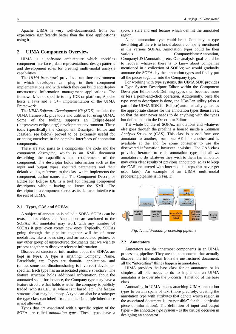
The whole bundle of SOFAs, annotations and whatever

else goes through the pipeline is housed inside a Common

Analysis Structure (CAS). This class is passed from one

annotator to another, from one AE into another and is

available at the end for some consumer to use the

discovered information however it wishes. The CAS class

provides iterators to each annotation type and allows

annotators to do whatever they wish to them (an annotator

may even clear results of previous annotators, so as to keep

the CAS uncluttered with intermediate steps that never get

used later). An example of an UIMA multi-modal

processing pipeline is in Fig. 1:

Fig. 1: multi-modal processing pipeline

2.2 Annotators

Annotators are the innermost components in an UIMA

processing pipeline. They are the components that actually

discover the information from the unstructured document:

all the “interesting” things happen in annotators.

UIMA provides the base class for an annotator. At its

simplest, all one needs to do to implement an UIMA

annotator is to override the process(...) method of the base

class.

Annotating in UIMA means attaching UIMA annotation

types to certain spans of text (more precisely, creating the

annotation type with attributes that denote which region in

the associated document is “responsible” for this particular

piece of information). The definition of input and output

types – the annotator type system – is the critical decision in

designing an annotator.

6 J. Hajic jr., K. Veselovská

Annotators have two sources of information they can

work with: the CAS that runs through the pipeline, from

which an annotator gets the document and previously done

annotations, and the UIMA Context class, which contains

additional information about the environment the annotator

is run in: various external resources, configuration

parameters, etc. All the inputs an annotator needs to run are

described in its component descriptor.

An example annotator could be a tokenizer, an annotator

responsible for segmenting text into tokens. It may simply

delimit tokens, or it may also add features such as lemma,

part of speech, etc. The simpler annotator will require

nothing and output the type, let's say, TokenAnnotation

with only the span defined and no associated features. The

more complex tokenizer will require no input types and

maybe an outside resource with a trained statistical model

for lemmatization and POS tagging; it will output the type

ComplexTokenAnnotation with a feature structure

containing the lemma and part of speech features. Maybe

the annotators should require an input LanguageAnnotation

type that is associated with the whole document and its

feature structure has a language feature, containing some

pre-defined language code, so that the tokenizer knows

which statistical model to load. This LanguageAnnotation

might be the output of a language recognition algorithm

implemented by another annotator further up the pipeline.

There can instead be a LanguageSpanAnnotation type can

also be designed to allow for multi-lingual documents, by

actually giving it a span. The Tokenizer will then iterate

over those LanguageSpanAnnotations and will load a

different model for each of them, etc.

This example only illustrates the flexibility and ease of

use for UIMA: other than the type system, there is no

restriction on what the components actually do inside. The

input and output of annotators is standardized by the UIMA

framework, so that if you think you have a better language

identifier which uses a completely different algorithm, you

can plug it in and as long as it keeps outputting the

LanguageAnnotation type, nothing needs to be changed for

the tokenizer. This is no magic – any good programmer

knows how to keep things modular – but the point is,

UIMA already does this for free, and with a great amount

of generality.

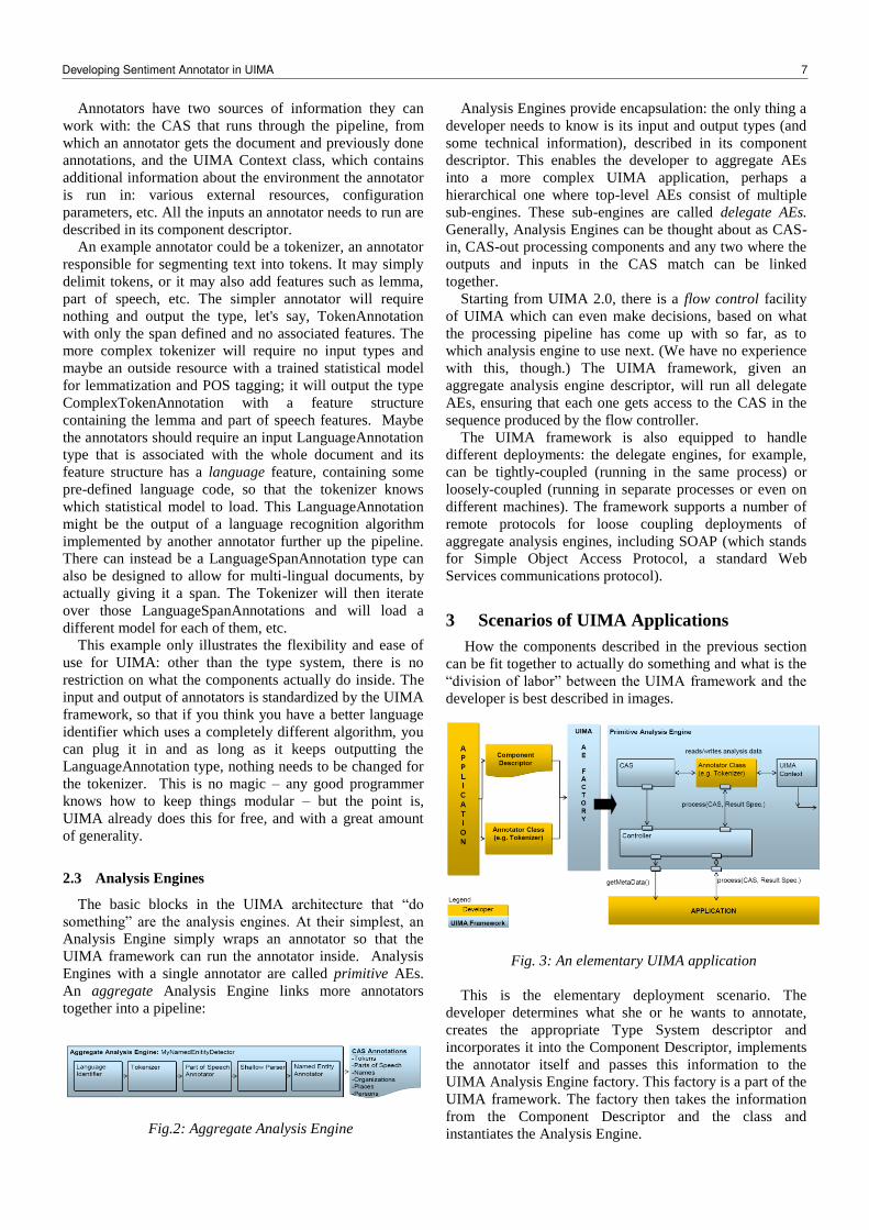
2.3 Analysis Engines

The basic blocks in the UIMA architecture that “do

something” are the analysis engines. At their simplest, an

Analysis Engine simply wraps an annotator so that the

UIMA framework can run the annotator inside. Analysis

Engines with a single annotator are called primitive AEs.

An aggregate Analysis Engine links more annotators

together into a pipeline:

Fig.2: Aggregate Analysis Engine

Analysis Engines provide encapsulation: the only thing a

developer needs to know is its input and output types (and

some technical information), described in its component

descriptor. This enables the developer to aggregate AEs

into a more complex UIMA application, perhaps a

hierarchical one where top-level AEs consist of multiple

sub-engines. These sub-engines are called delegate AEs.

Generally, Analysis Engines can be thought about as CAS-

in, CAS-out processing components and any two where the

outputs and inputs in the CAS match can be linked

together.

Starting from UIMA 2.0, there is a flow control facility

of UIMA which can even make decisions, based on what

the processing pipeline has come up with so far, as to

which analysis engine to use next. (We have no experience

with this, though.) The UIMA framework, given an

aggregate analysis engine descriptor, will run all delegate

AEs, ensuring that each one gets access to the CAS in the

sequence produced by the flow controller.

The UIMA framework is also equipped to handle

different deployments: the delegate engines, for example,

can be tightly-coupled (running in the same process) or

loosely-coupled (running in separate processes or even on

different machines). The framework supports a number of

remote protocols for loose coupling deployments of

aggregate analysis engines, including SOAP (which stands

for Simple Object Access Protocol, a standard Web

Services communications protocol).

3 Scenarios of UIMA Applications

How the components described in the previous section

can be fit together to actually do something and what is the

“division of labor” between the UIMA framework and the

developer is best described in images.

Fig. 3: An elementary UIMA application

This is the elementary deployment scenario. The

developer determines what she or he wants to annotate,

creates the appropriate Type System descriptor and

incorporates it into the Component Descriptor, implements

the annotator itself and passes this information to the

UIMA Analysis Engine factory. This factory is a part of the

UIMA framework. The factory then takes the information

from the Component Descriptor and the class and

instantiates the Analysis Engine.

Developing Sentiment Annotator in UIMA 7

The UIMA framework provides methods to support the

application developer in creating and managing CASes and

instantiating, running and managing AEs. However, since

our work is only to implement the annotator class and

provide the descriptor into an IBM application, we have no

experience with actually using an Analysis Engine.

3.1 Collection Processing

Typically, the application will be processing multiple

documents, a collection. This presents additional challenges

in creating a collection reader and managing the iterative

workflow (distributed processing, error recovery, etc.)

Almost any UIMA application will have a source-to-sink

workflow like in Fig. 3:

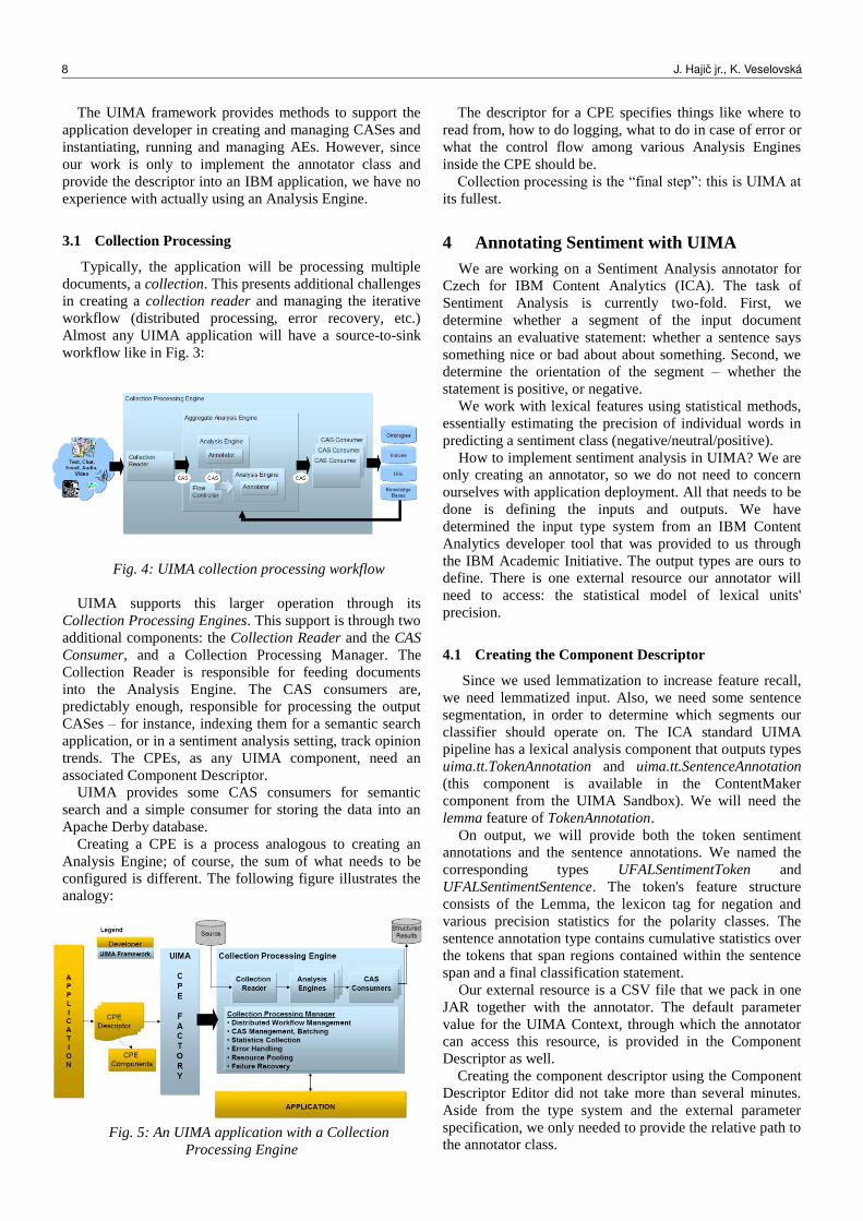
Fig. 4: UIMA collection processing workflow

UIMA supports this larger operation through its

Collection Processing Engines. This support is through two

additional components: the Collection Reader and the CAS

Consumer, and a Collection Processing Manager. The

Collection Reader is responsible for feeding documents

into the Analysis Engine. The CAS consumers are,

predictably enough, responsible for processing the output

CASes – for instance, indexing them for a semantic search

application, or in a sentiment analysis setting, track opinion

trends. The CPEs, as any UIMA component, need an

associated Component Descriptor.

UIMA provides some CAS consumers for semantic

search and a simple consumer for storing the data into an

Apache Derby database.

Creating a CPE is a process analogous to creating an

Analysis Engine; of course, the sum of what needs to be

configured is different. The following figure illustrates the

analogy:

Fig. 5: An UIMA application with a Collection

Processing Engine

The descriptor for a CPE specifies things like where to

read from, how to do logging, what to do in case of error or

what the control flow among various Analysis Engines

inside the CPE should be.

Collection processing is the “final step”: this is UIMA at

its fullest.

4 Annotating Sentiment with UIMA

We are working on a Sentiment Analysis annotator for

Czech for IBM Content Analytics (ICA). The task of

Sentiment Analysis is currently two-fold. First, we

determine whether a segment of the input document

contains an evaluative statement: whether a sentence says

something nice or bad about about something. Second, we

determine the orientation of the segment – whether the

statement is positive, or negative.

We work with lexical features using statistical methods,

essentially estimating the precision of individual words in

predicting a sentiment class (negative/neutral/positive).

How to implement sentiment analysis in UIMA? We are

only creating an annotator, so we do not need to concern

ourselves with application deployment. All that needs to be

done is defining the inputs and outputs. We have

determined the input type system from an IBM Content

Analytics developer tool that was provided to us through

the IBM Academic Initiative. The output types are ours to

define. There is one external resource our annotator will

need to access: the statistical model of lexical units'

precision.

4.1 Creating the Component Descriptor

Since we used lemmatization to increase feature recall,

we need lemmatized input. Also, we need some sentence

segmentation, in order to determine which segments our

classifier should operate on. The ICA standard UIMA

pipeline has a lexical analysis component that outputs types

uima.tt.TokenAnnotation and uima.tt.SentenceAnnotation

(this component is available in the ContentMaker

component from the UIMA Sandbox). We will need the

lemma feature of TokenAnnotation.

On output, we will provide both the token sentiment

annotations and the sentence annotations. We named the

corresponding types UFALSentimentToken and

UFALSentimentSentence. The token's feature structure

consists of the Lemma, the lexicon tag for negation and

various precision statistics for the polarity classes. The

sentence annotation type contains cumulative statistics over

the tokens that span regions contained within the sentence

span and a final classification statement.

Our external resource is a CSV file that we pack in one

JAR together with the annotator. The default parameter

value for the UIMA Context, through which the annotator

can access this resource, is provided in the Component

Descriptor as well.

Creating the component descriptor using the Component

Descriptor Editor did not take more than several minutes.

Aside from the type system and the external parameter

specification, we only needed to provide the relative path to

the annotator class.

8 J. Hajic jr., K. Veselovská

4.2 Code

Creating the annotator code then consisted of running the

JCasGen utility to generate from the type system the

classes that go into the CAS as annotations and writing the

algorithm itself. The only UIMA-specific code that had to

be written raw was reading from the CAS and adding

annotations to it (no more than some 10 lines of code). On

the UIMA side, development was easy; on the IBM side,

we are still encountering interoperability issues.

5 Conclusions

Our experience with UIMA is not very extensive:

currently, our task is simply to implement a sentiment

annotator for the IBM Content Analytics application.

However, according to our up-to-date knowledge of the

system, we are convinced that UIMA is a very thorough,

flexible and robust framework. Moreover, the

documentation of UIMA is extremely good.

The UIMA SDK does its utmost to relieve the developer

of tedious, repetitive tasks through utilities like the

JCasGen and the Component Descriptor Editor, as long as

the Eclipse IDE is used. These utilities make it easy to start

working with UIMA. The SDK does its best to help the

developer focus on the meaningful parts of the task at hand

only: on implementing the algorithms that discover

information inside the unstructured data.

This is, we feel, the greatest contribution of UIMA:

standardizing and automating the common parts of more or

less any data mining application and providing an easy

enough way of filling in the “interesting bits”, while at the

same time being flexible enough to meet most application

demands (multi-modality, complex control flow, etc.) At

the same time, it also provides robust runtime capabilities.

Also, UIMA aggregate AEs enable and encourage

granularity, so individual annotators can be designed so

that they do not require more than one person to implement

them reasonably fast. Therefore, once the component

descriptors are agreed upon, teamwork should be easy.

A weak point may be flexibility on the programmer side:

as soon as one strays from a development scenario where

the UIMA SDK tools are useful, the amount of work

necessary to get an UIMA application up and running

increases dramatically. We also do not know how

complicated it is to administer an UIMA application.

UIMA might not be the framework of choice in an

academic, experimental setting, since it provides no

facilities for evaluating the performance of the data mining

algorithms inside and is probably unnecessarily complex

for most experimental scenarios. Implementing such an

evaluator, however, might not be too difficult, either as an

external application operating on the database one of the

available CAS consumers generates, or as an UIMA

component, using some of the semantic search CAS

consumers. Furthermore, given UIMA flexibility,

modularity and re-usability, if such an evaluation

component was present, an UIMA CPE could be a great

way of testing data mining algorithms in various complex

settings.

We are convinced that UIMA is worth knowing about.

Acknowledgment

The work on this project has been supported by IBM

Academic Initiative program. Text and images from the

UIMA documentation

(http://uima.apache.org/documentation.html) have been

used. The sentiment analysis research is also supported by

the GAUK 3537/2011 grant and by SVV project number

267 314.

Developing Sentiment Annotator in UIMA 9

Transformation of GUHA association rules to business rules

for implementation using JBoss Drools

Stanislav Vojíř

Department of Knowledge Engineering

University of Economics, Prague

W. Churchill Sq. 4, Prague 3, 130 67, Czech Republic

Abstract. Data mining of association rules is one way of finding interesting relationships in data - especially in the case of using GUHA method. These rules have not been used only to description but also to learn the preferences of users and used like decision rules in the form of business rules. The following paper presents a transformation from GUHA association rules to DRL form of business rules and using of them in business rules system JBoss Drools. The paper also outlines some possibilities of interpretation of association rules in the form of business rules and possible solving of transformation problems (with uniqueness, entity identification and best results selection).

1 Motivation and problem definition

If we consider the environment of information systems,

we cannot ignore their growing complexity and integration.

With the increasing complexity it grows also the efforts to

better separation of business logic from application code

itself. For this purpose some specialized formats for saving

and exchange of business logic get more and more popular.

These formats are collectively called “business rules”.

Business rules may be stored in many forms (text,

structured data, diagrams…) and formats. We can find

quite a lot of specifications of them – SBVR, SWRL etc.

(see 2.2) These specifications have different expressive

power, but it is possible to say, that all the final formats are

quite easy to understand. The disadvantage of business

rules is that in most cases they have to be written manually.

For example it is necessary to have an expert for the

domain of “client preferences”.

On the other side, many companies usually have quite

much data about behavior of their clients. With a little

exaggeration it could be said that almost every bigger

company collects data about its own customers (clients).

The behavior of clients is driven by their preferences and

these preferences should in an ideal case be the same

preferences, which are hidden in the domain knowledge

written in business rules.

The author of this paper believes that it is possible to

extract the domain knowledge (described above) from data

using descriptive method of data mining – association

rules. Association rules may be not only concerned on the

problem of shopping cart. We can use the GUHA method,

more precisely the GUHA association rules [4] extracted

using software LISp-Miner [2][3].

GUHA Association rules have a great expressive power,

but they are quite difficult interpretable. And of course,

these rules cannot be directly executed – they only describe

the reality. The data mining expert usually has to write a

long analytical report with information of data

preprocessing, particular questions and finally about

founded association rules and their impact on the business.

Then there must be a domain expert, which reads the

results of analytical report and “rewrites” some of the

results into domain knowledge base (in any form of

business rules).

It would be very useful if we could semi-automatically

convert founded association rules into the form of business

rules.1 But this problem is not so easy how it could look

out. It is not possible to write a simple transformation from

association rules to business rules. It is necessary to solve

some partly problems, which have to be solved during the

transformation process.

The following text is divided into these sections: 2 –

Business rules in information systems, 3 – Execution of

business rules based on GUHA association rules, 4 – The

uniqueness of entities and their relationships, 5 – Problem

of conflicting rules and 6 – Conclusion and future work.

2 Business rules in information systems

2.1 Business rules – in general

“Business rule” in a general meaning is a rule for

business, but in informatics (and of course in this paper,

too), we use extended definition. Business rules are a way

of separation of business and application logic of an

information system or business application. These rules are

used for two different purposes: for saving and exchange of

“business know how” and for “decision making and

reactions to events” in an application.

We can speak about three different types of business

rules [6]:

declaration business rules – term (entity, relation…)

declarations

descriptive business rules – declaration of relations

between terms and term derivation

action business rules – execution of actions like

reaction on change in inference base (inference tree

in business rule system)

2.2 Format of business rules

Business rules can be created and saved in different

forms and their relevant formats. Regarding the forms we

can nominate: text form (semi-natural language like Simple

English in SBVR), structured text form (mostly used,

specialized dialects like DRL, Jess etc.), diagrams (UML

form of SBVR), XML or ontology (SBVR, SWRL and

more others) and decision tables (used by many rule

engines). And we can complete the previous list with the

rules written in some programming language.

1 The suitability of this conversion was also syndicated

on the occasion of presentation of tool I:ZI Miner on

conference ECML-PKDD 2012. [5]

ITAT 2013: Workshops, Posters, and Tutorials, pp. 10–14ISBN 978-1490952086, c© 2013 S. Vojír

Too many forms, too many formats and dialect – it is a

big problem for selection of one “best” language for

business rules. When we look at business rules engine and

components for their inclusion (or connection) into

information systems, we have to say, that fast each rule

engine uses another form of rules. And some business rule

formats are very well described but there is no existing

implementation.

For example the language Semantics of Business

Vocabulary and Business Rules (SBVR) [1] is a standard,

which has four possible forms. These forms are described

in one document, but they are not fully compatible and

have different expression power. And for some of them

there are no existing execution engines.

2.3 Choise of business rule language and execution

engine

Performed background researches of business rules

execution and management system gave us a closer range

of languages and engines for selection.

The author wants to use as the main execution engine

JBoss Drools. [7] This business rules engine is distributed

as open source and written in java. It supports basic

operations for adding rules to the derivation rule base and

execution of them on a set of entities saved in inference

tree. The entities could be changed during the evaluation

and each activated rule could work with java objects. The

rules are (a little simplified) in the form (in DRL language):

rule <name of rule>

when <condition>

then <some action> end.

JBoss Drools as a base component does not support

management of the rules themselves. It could be an

advantage for modification of management for using in

combination of data mining results. [8]

For administration of business rules by lay users

(management of a company etc.), rules in DRL form are

still too complicated. For this purpose the author would like

to use “Simpler English” form of SBVR. [1]

For connection to ontologies (for example for deriving

on the semantic web) could be a good choice the language

Semantic Web Rule Language (SWRL). [10]

When we want (or have to) combine more languages of

business rules, which are not directly convertible between

themselves, we must be able to map entities with values

from each form to another one. It is necessary to use unique

entity names etc. – more in the section 4.

2.4 Generation of business rules

The main idea of business rules deals with the think, that

business rules should be defined by domain (business)

experts. The definition could be made by writing of

definition of business rules, setting-up business rules in the

form of parameters of business processes (in BPEL etc.),

using graphical definition tools, or in tables in Excel

spreadsheets.

But the domain of business rules is currently being quite

much studied (world-wide) and one of the targets of the

research is automatic generation of business rules. Other

groups which are interested in generation of business rules

on the base of collected data are working for example in

IBM (at least according to interviews with some of their

members). Some research teams try to extract business

rules from plaintext (textual description of business

processes), other from data mining results. But the author

has not found publications about generation of business

rules from association rules.

3 Execution of business rules based on

GUHA association rules

If we want to speak about conversion of GUHA

association rules into business rules in DRL form (for

JBoss Drools), we have to introduce the both types of these

rules. For simplification we could use an example of

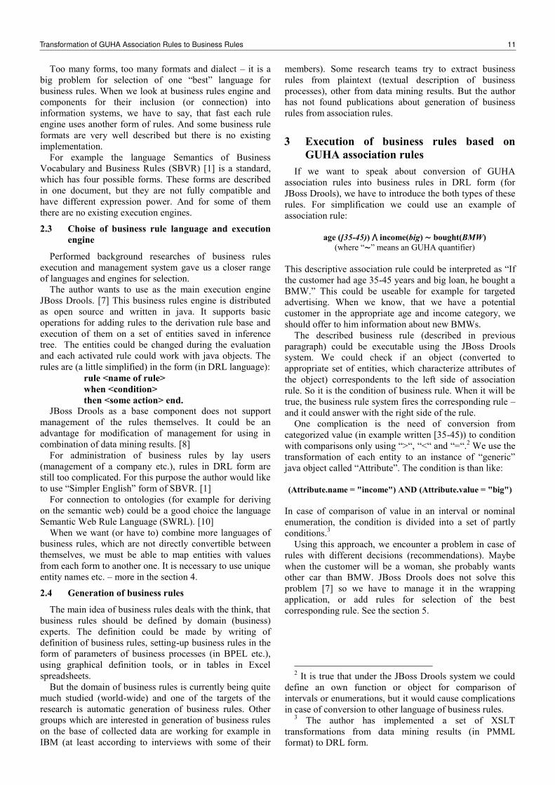
association rule:

age ([35-45)) ⋀ income(big) ∼ bought(BMW)

(where “∼” means an GUHA quantifier)

This descriptive association rule could be interpreted as “If

the customer had age 35-45 years and big loan, he bought a

BMW.” This could be useable for example for targeted

advertising. When we know, that we have a potential

customer in the appropriate age and income category, we

should offer to him information about new BMWs.

The described business rule (described in previous

paragraph) could be executable using the JBoss Drools

system. We could check if an object (converted to

appropriate set of entities, which characterize attributes of

the object) correspondents to the left side of association

rule. So it is the condition of business rule. When it will be

true, the business rule system fires the corresponding rule –

and it could answer with the right side of the rule.

One complication is the need of conversion from

categorized value (in example written [35-45)) to condition

with comparisons only using “>“, “<“ and “=“.2 We use the

transformation of each entity to an instance of “generic”

java object called “Attribute”. The condition is than like:

(Attribute.name = "income") AND (Attribute.value = "big")

In case of comparison of value in an interval or nominal

enumeration, the condition is divided into a set of partly

conditions.3

Using this approach, we encounter a problem in case of

rules with different decisions (recommendations). Maybe

when the customer will be a woman, she probably wants

other car than BMW. JBoss Drools does not solve this

problem [7] so we have to manage it in the wrapping

application, or add rules for selection of the best

corresponding rule. See the section 5.

2 It is true that under the JBoss Drools system we could

define an own function or object for comparison of

intervals or enumerations, but it would cause complications

in case of conversion to other language of business rules. 3 The author has implemented a set of XSLT

transformations from data mining results (in PMML

format) to DRL form.

Transformation of GUHA Association Rules to Business Rules 11

4 The uniqueness of entities and their

relationships

A problem of transformation of real-world data into

exchangeable form is that there are many names for entities

with the same meaning. In this part of the article we focus

on some possible approaches to solving this problem.

4.1 Entity name and identification

Almost all formats of business rules are based on some

entities (objects extracted from real-world). These entities

have some attributes, which can be compared with the

specification saved in business rules. When we work with

standardized data from one dataset, everything should be

OK. The domain expert should use one data vocabulary and

every entity should have the same meaning in every rule, in

which it is used, etc. But we want to generate business rules

from data-mining results. And these data can have various

names and categories of values. The best is to put the

problem in the example:

We have data-table with column “age”. This column

contains values of age of people. (It does not matter in what

context with other columns.) We want to save one business

rule containing: “Customers under 15 years usually buy

<something>.” The domain expert could know this

preference and knows that age must be specified in years as

a number. Also he should write something like “age < 15“.

But the data-table was used for data-mining and the domain

expert receives some underlying association rules with

contents (entities) “80% of children” and “young

customers” What does it mean? The domain expert have to

read the full content of the analytical report and look out,

how old are the “young customers” and what was meant by

the entity “children”.

In some formats (languages) of business rules, these

named entities can be described in a separate set of rules

and after that the entities can be used in other business

rules. But if we apply this approach often, it will result in

too complex set of business rules (because of the large

number of labels for similar entities).

The better approach is using of only one label (name) for

each entity. We could easily say that the domain expert (or

semi-automatic system) should do re-preprocessing of data-

table and use the original column name and values for

expression of the rule. The prize will be an extending of

processed rules and it does not solve the problem of more

analytical reports based on different data-tables. The

domain or analytical expert should use only entity names

from a “company vocabulary”?

It would be nice when the domain expert could use his

own preferred set of entities in connection with entities

used in data-mining results, dataset and other business rules

in the domain knowledge base.

4.2 “Dictionaries” of entity names

As outlined in the preceding paragraphs for using of

business rules it is necessary to use only one set of entities,

which are used in conditions or actions of business rules.

Event when using of “class definition” in SBVR or SWRL,

the business rules engine must be able to translate the

entities used in business rules to their base form with

unique names.

4.2.1 Relational database

If we look at the world of relational databases (because

the data-tables used for data mining are usually saved in

relational databases), one solution could be very easy. We

could create one table for names of entities. This table

could have a column (primary key) for “name” and other

column for alternative name. The same could be done for

relational-connected table (or tables) for mapping of values.

This approach should work, it could be useable for

transformation from association rules or data values for

using in business rules engine. The disadvantage of this

approach could be the big growth of size of this mapping

tables and this solution would be only hardly administrable.

4.2.2 Entities from an ontology

Other approach for identification of entities used in rules

could be “matching to entities in any ontology”. Ontologies

are currently one of the popular topics related to semantic

in information systems. They help their users to unify the

concepts used in communication and data exchange.

In the world of languages and formats for business rules,

we can find the Semantic Web Rule Language (SWRL),

which is based on ontological expressions [11]. It expects

to use entities defined as concepts in any ontology. The

author of this paper believes that it could be useable for

solving of the problem of ambiguity of names of entities.

We could extend this approach for mapping of values (and

categories of them) used in data-table, rules etc. This

extension could be connected with a knowledge base used

for data-mining – see the following chapter.

4.2.3 Background knowledge for data mining

In the SEWEBAR Project, we deal with background

knowledge base for data mining. We collect information

about data formats and their preprocessing. We are using a

proprietary format called BKEF4 (based on XML). We

know that it is necessary to have information about each

type of entity (column in data table) - in connection with

BKEF, we call it “meta-attribute”. Each meta-attribute

could have more formats with different scales of values and

each format could have more definitions of preprocessing

for data mining. [15] We are working with semi-automatic

mapping of these meta-attributes and their formats to data-

tables before start of the data mining using I:ZI Miner.5 [5]

The problem is that we usually have one BKEF file for

each data table (sometimes for each analytical question).

The user can map the data table to an existing BKEF file,

but it is considerably simpler to input preprocessing

instructions via the web interface only for the one task. We

would like to complete the way of working with knowledge

base for data mining. In connection with this it would be

appropriate to use an approach which could be useable for

unified identification of entity types and their values in case

of business rules.

We could think that the better way could be using

ontology for knowledge base for data mining (including

information of formats and their values) [13]. We have to

extend the original concept of necessary information range.

4 Background knowledge exchange format

5 Web data mining solution based on LISp-Miner.

12 S. Vojír

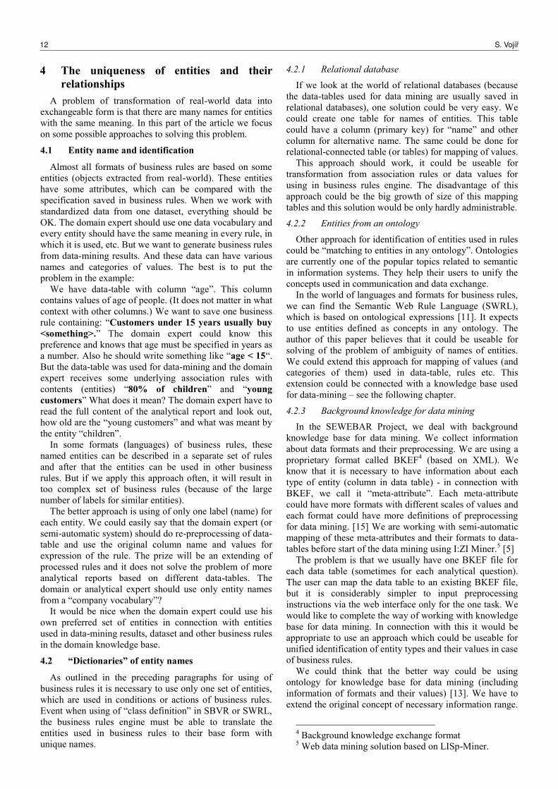
It should be possible to define relations between categories

of values. In reference to the example given in 4.1, there

should be possibilities to define relations like:

Fig. 1. Example: part of knowledge base for data mining

saved in ontology

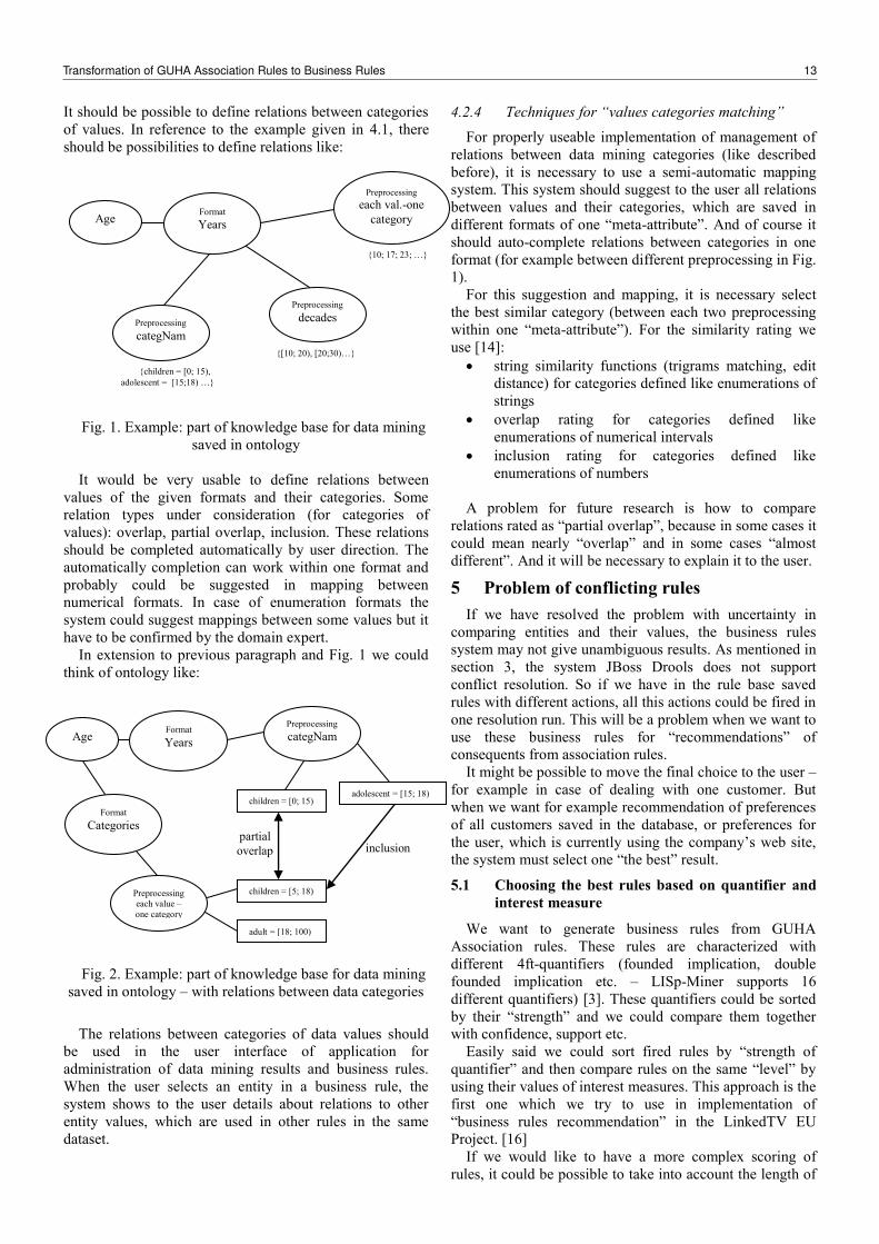
It would be very usable to define relations between

values of the given formats and their categories. Some

relation types under consideration (for categories of

values): overlap, partial overlap, inclusion. These relations

should be completed automatically by user direction. The

automatically completion can work within one format and

probably could be suggested in mapping between

numerical formats. In case of enumeration formats the

system could suggest mappings between some values but it

have to be confirmed by the domain expert.

In extension to previous paragraph and Fig. 1 we could

think of ontology like:

Fig. 2. Example: part of knowledge base for data mining

saved in ontology – with relations between data categories

The relations between categories of data values should

be used in the user interface of application for

administration of data mining results and business rules.

When the user selects an entity in a business rule, the

system shows to the user details about relations to other

entity values, which are used in other rules in the same

dataset.

4.2.4 Techniques for “values categories matching”

For properly useable implementation of management of

relations between data mining categories (like described

before), it is necessary to use a semi-automatic mapping

system. This system should suggest to the user all relations

between values and their categories, which are saved in

different formats of one “meta-attribute”. And of course it

should auto-complete relations between categories in one

format (for example between different preprocessing in Fig.

1).

For this suggestion and mapping, it is necessary select

the best similar category (between each two preprocessing

within one “meta-attribute”). For the similarity rating we

use [14]:

string similarity functions (trigrams matching, edit

distance) for categories defined like enumerations of

strings

overlap rating for categories defined like

enumerations of numerical intervals

inclusion rating for categories defined like

enumerations of numbers

A problem for future research is how to compare

relations rated as “partial overlap”, because in some cases it

could mean nearly “overlap” and in some cases “almost

different”. And it will be necessary to explain it to the user.

5 Problem of conflicting rules

If we have resolved the problem with uncertainty in

comparing entities and their values, the business rules

system may not give unambiguous results. As mentioned in

section 3, the system JBoss Drools does not support

conflict resolution. So if we have in the rule base saved

rules with different actions, all this actions could be fired in

one resolution run. This will be a problem when we want to

use these business rules for “recommendations” of

consequents from association rules.

It might be possible to move the final choice to the user –

for example in case of dealing with one customer. But

when we want for example recommendation of preferences

of all customers saved in the database, or preferences for

the user, which is currently using the company’s web site,

the system must select one “the best” result.

5.1 Choosing the best rules based on quantifier and

interest measure

We want to generate business rules from GUHA

Association rules. These rules are characterized with

different 4ft-quantifiers (founded implication, double

founded implication etc. – LISp-Miner supports 16

different quantifiers) [3]. These quantifiers could be sorted

by their “strength” and we could compare them together

with confidence, support etc.

Easily said we could sort fired rules by “strength of

quantifier” and then compare rules on the same “level” by

using their values of interest measures. This approach is the

first one which we try to use in implementation of

“business rules recommendation” in the LinkedTV EU

Project. [16]

If we would like to have a more complex scoring of

rules, it could be possible to take into account the length of

10; 17; 23; …

Age Format Years

Preprocessing

each val.-one

category

Preprocessing

decades

[10; 20), [20;30)…

Preprocessing

categNam

children = [0; 15),

adolescent = [15;18) …

Age Format Years

Preprocessing

categNam

children = [0; 15) adolescent = [15; 18)

Format Categories

Preprocessing

each value –

one category

children = [5; 18)

adult = [18; 100)

inclusion partial

overlap

Transformation of GUHA Association Rules to Business Rules 13

antecedent of association rule. We can say that the longer

condition should be more precise than the shorter one, but

it is necessary to compare it together with interest

measures. And the answer to the question: “Which rule is

better?” is really not easy. We would like to deal with it in

the future work.

5.2 Rules rating

Other approach for selection of best result

recommendation could be rating of individual business

rules. This way is usually used in user-filled business rules

system. The user can set up order of saved rules and the

system results the first founded result.

Maybe it could be also possible to join this approach to

our system. In the future the user should be able to edit and

manage the set of saved association rules and so it could be

possible to give to the user a possibility to sort them.

Other way for completion of rating for individual rules

could be collecting of feedback. When we run the system

automatically on the web we should be able to check if the

recommendation of user preferences are good or bad. For

example in LinkedTV project we could check if the user

plays the recommended video. So the business rules

component could be followed by a simple machine learning

system for correction of conflicting rules.

5.3 LinkedTV implementation

The closest target is a connection of the first

implementation into LinkedTV Gain project, where the

business rule module should be used for recommendation

of user preferences to selected videos and web pages.

LinkedTV is an EU project, which is targeted on

recommendation rich contextual content for videos, TV

stream and web pages. Each part of video stream is

annotated with entities like “sport”, “city”, “person” etc.

and the application collects information about reactions of

the watcher (skipping parts of the video stream, going

out…). On the base of this dataset we can mine association

rules about preferences of the user. Finally, after the

conversion into business rules, these rules will be used for

recommendation, if a concrete annotated video is suitable

for the current user. It means, that when a user usually

watches sport programs and skips programs about “news”,

the recommendation system should suggest to him some

videos with similar sport context.

6 Conclusion and future work

The author would like to describe a model of

transformation from GUHA association rules into business

rules and develop a sample implementation of the decision

system using generated business rules. The work is

currently in progress.

For the using in LinkedTV Project, it will be suitable to

implement a hybrid system, which combines

recommendations on the base of the preferences of the

current user, base of shared user preferences and a machine

learning algorithm.

References

[1] OMG (Object management group), “Semantics of

Business Vocabulary and Business Rules (SBVR),

v1.0.,” SBVR 1.0. [Online] 2. 1. 2008 [Cited:

13. 1. 2012] http://www.omg.org/spec/SBVR/1.0/PDF

[2] M. Šimůnek, “Academic KDD Project LISp-Miner,”

Intelligent Systems Design and Applications. 2003,

vol. 23, pages 263-272.

[3] “The official site of the LISp-Miner project” [Online]

[Cited: 1. 6. 2013] http://lispminer.vse.cz/

[4] J. Rauch, M. Šimůnek, “An Alternative Approach to

Mining Association Rules,” Foundations of Data

Mining and knowledge Discovery. 2005, Sv. 6,

stránky 211-231.

[5] R. Škrabal, M. Šimůnek, S. Vojíř, A. Hazucha, T.

Marek, D. Chudán, T. Kliegr, “Association Rule

Mining Following the Web Search Paradigm,”

ECML-PKDD 2012, Berlin: Springer, 2012, p. 808--

811. ISBN 978-3-642-33486-3

[6] Business rules group, “Defining Business Rules ~

What Are They Really?” [Online] [Cited: 20. 5. 2013]

http://www.businessrulesgroup.org/first_paper/br01c3

.htm

[7] “Drools,” JBoss Community [Online] [Cited: 1. 5.

2013] http://www.jboss.org/drools/

[8] “JBoss Drools Tutorial – drools,” JBoss application

server tutorials. [Online] [Cited: 1. 4. 2013]

http://www.mastertheboss.com/drools/jboss-drools-

tutorial

[9] B-TU Cottbus, “Using Drools: UServ Product derby

2005,” [Online] 18. 9. 2008 [Cited: 17. 12. 2011]

http://hydrogen.informatik.tu-

cottbus.de/wiki/index.php/Userv

[10] W3C, „SWRL: A Semantic Web Rule Language”

[Online] http://www.w3.org/Submission/SWRL/

[11] I. Horrocks, et al. “SWRL: A Semantic Web Rule

Language Combining OWL and RuleML” [Online]

19. 11. 2003 [Citace: 15. 11. 2011]

http://www.daml.org/2003/11/swrl/

[12] N. Abadie, “Schema Matching Based on Attribute

Values and Background Ontology,”. Leibniz

Universität Hannover, Germany : 2009, 12th AGILE

International Conference on Geographic Information

Science 2009

[13] T. Kliegr, S. Vojíř, J. Rauch, “Background knowledge

and PMML: first considerations,” San Diego,

California, USA : ACM, 2011. Proceedings of the

2011 workshop on Predictive markup language

modeling. 978-1-4503-0837-3.

[14] S. Vojíř, T. Kliegr, V. Svátek, O. Zamazal,

“Automated matching of data mining dataset

schemata to background knowledge,” Bonn: 2011,

ISWC 2011, ISSN 1613-0073

[15] J. Rauch, J., M. Šimůnek, “Dealing with Background

Knowledge in the SEWEBAR Project,” Knowledge

Discovery Enhanced with Semantic and Social

Information. Studies in Computational Intelligence,

2009, Vol. 220, pp. 89-106.

[16] LinkedTV, “Television linked to the web,” [Online]

[Cited: 1. 6. 2013] http://www.linkedtv.eu

14 S. Vojír

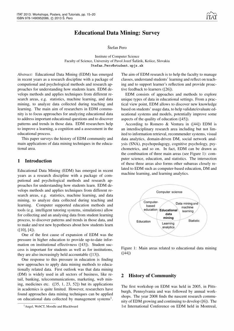
Educational Data Mining: Survey

Štefan Pero

Institute of Computer ScienceFaculty of Science, University of Pavol Jozef Šafárik, Košice, Slovakia

Stefan.Pero@student.upjs.sk

Abstract: Educational Data Mining (EDM) has emergedin recent years as a research discipline with a package ofcomputional and psychological methods and research ap-proaches for understanding how students learn. EDM de-velops methods and applies techniques from different re-search areas, e.g. statistics, machine learning, and datamining, to analyze data collected during teaching andlearning. The main aim of researchers in EDM commu-nity is to focus approaches for analyzing educational datato address important educational questions and to discoverpatterns and trends in those data. EDM researchers helpto improve a learning, a cognition and a assessment in theeducational process.

This paper surveys the history of EDM community andmain applications of data mining techniques in the educa-tional area.

1 Introduction

Educational Data Mining (EDM) has emerged in recentyears as a research discipline with a package of com-putional and psychological methods and research ap-proaches for understanding how students learn. EDM de-velops methods and applies techniques from different re-search areas, e.g. statistics, machine learning, and datamining, to analyze data collected during teaching andlearning. Computer supported education methods andtools (e.g. intelligent tutoring systems, simulations) allowfor collecting and an analysing data from student learningprocess, to discover patterns and trends in those data, andto make and test new hypotheses about how students learn([10], [4]).

One of the first cause of expansion of EDM was thepressure in higher education to provide up-to-date infor-mation on institutional effectivness ([43]). Student suc-cess is important for students as well as for institutions,they are also increasingly held accountable ([13]).

One response to this pressure in education is findingnew approaches to apply data mining methods to educa-tionally related data. First outlook was that data mining(DM) is widely used in all sectors of business, like re-tail, banking, telecommunications, marketing, web min-ing, medicines etc. ([35, 1, 23, 52]) but its applicationsin academics is quite limited. However, researchers havefound approaches data mining techniques can be appliedon educational data collected by management systems1.

1Angel, WebCT, Moodle and Blackboard

The aim of EDM research is to help the faculty to manageclasses, understand students’ learning and reflect on teach-ing and to support learner’s reflection and provide proac-tive feedback to learners ([26]).

EDM consists of appoaches and methods to exploreunique types of data in educational settings. From a prac-tical view point, EDM allows to discover new knowledgebased on students’ usage data, to help validate/evaluate ed-ucational systems and models, potentially improve someaspects of the quality of education ([45]).

According to Romero & Ventura in ([44]) EDM isan interdisciplinary research area including but not lim-ited to information retrieval, recommender systems, visualdata analytics, domain-driven DM, social network anal-ysis (SNA), psychopedagogy, cognitive psychology, psy-chometrics, and so on. In fact, EDM can be drawn asthe combination of three main areas (see Figure 1): com-puter science, education, and statistics. The intersectionof these three areas also forms other subareas closely re-lated to EDM such as computer-based education, DM andmachine learning, and learning analytics.

Figure 1: Main areas related to educational data mining([44])

2 History of Community

The first workshop on EDM was held in 2005, in Pitts-burgh, Pennsylvania and was followed by annual work-shops. The year 2008 finds the nascent research commu-nity of EDM growing and continuing to develop ([6]). The1st International Conference on EDM held in Montreal,

ITAT 2013: Workshops, Posters, and Tutorials, pp. 15–20ISBN 978-1490952086, c© 2013 Š. Pero

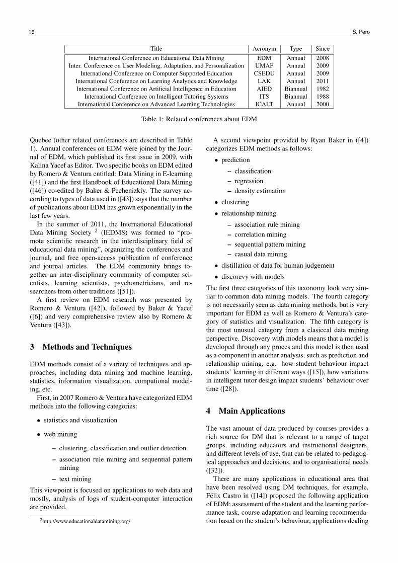
Title Acronym Type SinceInternational Conference on Educational Data Mining EDM Annual 2008

Inter. Conference on User Modeling, Adaptation, and Personalization UMAP Annual 2009International Conference on Computer Supported Education CSEDU Annual 2009

International Conference on Learning Analytics and Knowledge LAK Annual 2011International Conference on Artificial Intelligence in Education AIED Biannual 1982

International Conference on Intelligent Tutoring Systems ITS Biannual 1988International Conference on Advanced Learning Technologies ICALT Annual 2000

Table 1: Related conferences about EDM

Quebec (other related conferences are described in Table1). Annual conferences on EDM were joined by the Jour-nal of EDM, which published its first issue in 2009, withKalina Yacef as Editor. Two specific books on EDM editedby Romero & Ventura entitled: Data Mining in E-learning([41]) and the first Handbook of Educational Data Mining([46]) co-edited by Baker & Pechenizkiy. The survey ac-cording to types of data used in ([43]) says that the numberof publications about EDM has grown exponentially in thelast few years.

In the summer of 2011, the International EducationalData Mining Society 2 (IEDMS) was formed to “pro-mote scientific research in the interdisciplinary field ofeducational data mining”, organizing the conferences andjournal, and free open-access publication of conferenceand journal articles. The EDM community brings to-gether an inter-disciplinary community of computer sci-entists, learning scientists, psychometricians, and re-searchers from other traditions ([51]).

A first review on EDM research was presented byRomero & Ventura ([42]), followed by Baker & Yacef([6]) and very comprehensive review also by Romero &Ventura ([43]).

3 Methods and Techniques

EDM methods consist of a variety of techniques and ap-proaches, including data mining and machine learning,statistics, information visualization, computional model-ing, etc.

First, in 2007 Romero & Ventura have categorized EDMmethods into the following categories:

• statistics and visualization

• web mining

– clustering, classification and outlier detection

– association rule mining and sequential patternmining

– text mining

This viewpoint is focused on applications to web data andmostly, analysis of logs of student-computer interactionare provided.

2http://www.educationaldatamining.org/

A second viewpoint provided by Ryan Baker in ([4])categorizes EDM methods as follows:

• prediction

– classification– regression– density estimation

• clustering

• relationship mining

– association rule mining– correlation mining– sequential pattern mining– casual data mining

• distillation of data for human judgement

• discorevy with models

The first three categories of this taxonomy look very sim-ilar to common data mining models. The fourth categoryis not necessarily seen as data mining methods, but is veryimportant for EDM as well as Romero & Ventura’s cate-gory of statistics and visualization. The fifth category isthe most unusual category from a clasiccal data miningperspective. Discovery with models means that a model isdeveloped through any proces and this model is then usedas a component in another analysis, such as prediction andrelationship mining, e.g. how student behaviour impactstudents’ learning in different ways ([15]), how variationsin intelligent tutor design impact students’ behaviour overtime ([28]).

4 Main Applications

The vast amount of data produced by courses provides arich source for DM that is relevant to a range of targetgroups, including educators and instructional designers,and different levels of use, that can be related to pedagog-ical approaches and decisions, and to organisational needs([32]).

There are many applications in educational area thathave been resolved using DM techniques, for example,Félix Castro in ([14]) proposed the following applicationof EDM: assessment of the student and the learning perfor-mance task, course adaptation and learning recommenda-tion based on the student’s behaviour, applications dealing

16 Š. Pero

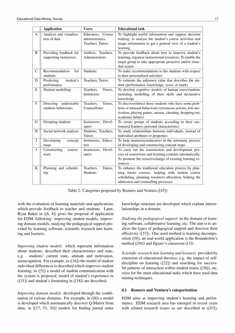
Application Users Educational taskA Analysis and visualiza-

tion of dataEducators, Courseadministrators,Teachers, Tutors

To highlight useful information and support decisionmaking; to analyse the student’s course activities andusage information to get a general view of a student’slearning

B Providing feedback forsupporting instructors

Authors, Teachers,Administrators

To provide feedback about how to improve student’slearning, organise instructional resources, To enable thetarget group to take appropriate proactive and/or reme-dial action

C Recommendation forstudents

Students To make recommendations to the students with respectto their personalised activities

D Predicting student’sperformance

Teachers, Tutors To estimate the unknown value that describes the stu-dent (performance, knowledge, score, or mark)

E Student modelling Teachers, Tutors,Instructors

To develop cognitive models of human users/studentsincluding modelling of their skills and declarativeknowledge

F Detecting undesirablestudents behaviours

Teachers, Tutors,Counsellours

To discover/detect those students who have some prob-lems or unusual behaviours (erroneous actions, low mo-tivation, playing games, misuse, cheating, dropping out,academic failure)

G Grouping students Instructors, Devel-opers

To create groups of students according to their cus-tomized features, personal characteristics

H Social network analysis Students, Teachers,Tutors

To study relationships between individuals, instead ofindividual attributes or properties

I Developing conceptmaps

Instructors, Educa-tors

To help instructors/educators in the automatic processof developing and constructing concept maps

J Constructing course-ware

Instructors, Devel-opers

To carry out the construction and development pro-cess of courseware and learning contents automatically,To promote the reuse/exchange of existing learning re-sources

K Planning and schedul-ing

Teachers, Tutors,Students

To enhance the traditional education process by plan-ning future courses, helping with student coursescheduling, planning resources allocation, helping theadmission and counselling processes

Table 2: Categories proposed by Romero and Ventura ([43])

with the evaluation of learning materials and applicationswhich provide feedback to teacher and students. Later,Ryan Baker in ([6, 4]) gives the proposal of applicationfor EDM, following: improving student models, improv-ing domain models, studying the pedagogical support pro-vided by learning software, scientific research into learn-ing and learners.

Improving student models which represent informationabout students, described their characteristics and state,e.g. students’ current state, attitude and motivation,metacognition. For example, in ([16]) the model of studentindividual differences is described which improves studentlearning; in ([5]) a model of student communication withthe system is proposed; model of student’s experience in([31]) and student’s frustrating in ([18]) are described.

Improving domain models developed through the combi-nation of various domains. For example, in ([8]) a modelis developed which automatically discover Q-Matrix fromdata; in ([17, 33, 34]) models for finding partial order

knowledge structure are developed which explain interre-lationships in a domain.

Studying the pedagogical support in the domain of learn-ing software, collaborative learning, etc. The aim is to an-alyze the types of pedagogical support and discover theireffectivity ([37]). One used method is learning decompo-sition ([9]), an real-world application is the Roundrobin’smethod ([56]) and Jigsaw’s classroom ([3]).

Scientific research into learning and learners provided byextension of educational theories, e.g. the impact of self-discipline on learning ([22]) and searching for success-ful patterns of interaction within student teams ([38]), etc.ories for the main educational tasks which have used datamining techniques.

4.1 Romero and Ventura’s categorization

EDM aims at improving student’s learning and perfor-mance. EDM research area has emerged in recent yearswith related research issues as are described in ([43]),

Educational Data Mining: Survey 17

shortly: 1) Analysis and visualization of data to help edu-cators to analyze students’ behaviour and learning ([57]),2) feedback for teachers, to help teachers in decision mak-ing ([27]), 3) recommendations for students the objectiveof what is to make pesonalized recommendations on learn-ing materials ([21]), 4) predicting student performance, topredict the likely performance of a student for given tasks([54]), and, 5) student modeling with the objective to de-velop cognitive models of a student, including skills andknowledges considering his characteristics (learning style,motivation, affective status and etc.) ([20, 2, 19]).

In ([32]) EDM applications are categorized into elevenareas according to Romero and Ventura ([43]), see the Ta-ble 2.

All these applications support learning process but fromthe perspective of the user (D), (G), (L), (M) are relatedto the organisation of learning, resources, grouping of stu-dents and organizing their schedule; (A), (B), (D), (E), (F),(H), (I) are focused especially on tutors, teachers and ed-ucators, even (H) focuses social network analysis. (C) isaimed only on students.

This categorization can be seen as the latest comprehen-sive classification of EDM applications, latest categoriza-tions are mostly derived, for instance in the Handbook ofEDM ([46]).

5 Educational Recommender Systems

Recommender systems (RSs) attempt to predict items fora user in which he might be interested. According to Ricciin ([40]) RSs are software tools and techniques providingsuggestions for items to be of use to a user. The recom-mendations relate to various decision-making processes,such as what products to buy, what music to listen, whatnews to read or what destination to choose for a trip, etc.

Specific and general terms of RSs are “item” and “user”.The “item ” is denoted what the system recommends tothe “user”. Items are selected from the specific domain(e.g. films, music, news or hotels) which determine thecore recommendation technique, graphical user interfacefor presentation of suggestions, etc.

RSs are very interesting for a company, e.g. to sell moreand diverse items, to increase users’ satisfaction and fi-delity, to better understand users’ needs. However, usershave also their own requirements on RSs, for example, tofind some good items with a relatively small effort, to ex-press herself by providing ratings or opinions, to help otherby contributing with information to the community ([25]).

RSs collect and exploit various types of informationabout users, items (products), and interactions betweenusers and items. The output of RSs is a personalized listof items which meets user’s needs (preferences). This in-formation may be gathered while the user is interactingwith the system, for instance, many times using the setof subjective ratings assigned by the users to previouslyexperienced items. These information serves the system

for predicting the rating for items not yet experienced. Fi-nally, the products with the highest ratings are then recom-mended to a user ([7]).

According to Burke, RSs techniques are classified intofour main categories: collaborative filtering, content basedfiltering, knowledge based filtering and hybrid systems([12]).

Collaborative filtering (CF) is a recommendation tech-nique which uses a simple social strategy called “word-of-mouth” ([24]). Personalized recommendations for thetarget user are sugessted using opinions of users havingsimilar tastes to those of the target user ([39]). CF tech-niques recognize similarities between users according totheir feedbacks and recommend items preferred by thelike-minded users ([25]). This is a domain independentapproach computed by leveraging historical log data ofusers’ online behaviour.

Content based filtering (CBF) is a recommendation tech-nique which suggests recommendations for a user by an-alyzing only the rating of the target user. CBF techniquesanalyze items’ descriptions to identify interesting items tothe target user ([36]). CBF techniques learn user’s inter-ests based on the features of items previously rated by theuser using supervised machine learning techniques ([25]).

Knowledge based filtering (KBF) techniques use a deci-sion model to make inferences about to the user needs.Usually KBF techniques compute some recommendationrules designed by the domain expert ([49]). KBF recom-mendations are based on knowledge about users’ needsand preferences ([25]).

Hybrid systems (HSs) combines several RSs techniquesto overcome limitations of pure techniques with betteraccuracy ([12, 50]). HSs are useful to integrate someadditional information to the system, for instance, providea way to integrate context into the prediction model ([7]).

Recently, RSs have shown to be sucessful in many do-mains where information overload exists. This success isalso a motivation for researchers to deploy RSs in educa-tional scenarious. The amount of data generated by stu-dents, teachers and educators during the learning processis so large that it is very difficult to understand to data.

Educational recommender systems (ERS) share thesame key objectives as RSs for e-commerce applications,for instance, to help users to select the best item from alarge information pool. However, there are some partic-ularities for which applying existing solutions from RSsapplications is not so straighforward, for instance, recom-mendations in the educational domain should not be sug-essted only by the learners’ preferences but also by edu-cational criteria. However, most ERS appoaches have fo-cused on applying traditional RSs techniques to find sug-gestions for students and teachers in the learning process([48]).

18 Š. Pero

According to Santos & Boticario, favorite topics of ERSare the following: knowledge modeling for the recom-mendation process ([55]); techniques and algorithms toproduce recommendations in e-learning settings ([53]);methodologies to develop ERS ([47]); architectures tosupport the recommendation process ([11]); evaluationmethods to measure the recommendations’ impact onusers ([30]); and application of ERS in real world scenari-ous ([29]).

6 Conclusion

EDM is a multidisciplinary research area consisting ofcomputer science, education, psychology, psychometricsand statistics to analyse, understand and answer educa-tional research questions. Increase in the usage of educa-tional software and monitoring tools of learning processesenabled to create large repositories of data reflecting howstudents learn. The main aim of community of EDM is tofocus approaches for analyzing those data to address im-portant educational questions and to discover patterns andtrends in those data. The same aim of researchers fromvarious research fields is to support the education, to betterunderstand and improve learning, and to provide informa-tion about the learning process.

References

[1] P. Adriaans and D. Zantinge. Data mining. Addison-Wesley, Boston, MA, 2005.

[2] S. Amershi and C. Conati. Combining unsupervised and su-pervised classification to build user models for exploratorylearning environments. Journal of Education Data Mining,pages 18–71, 2009.

[3] E. Aronson and S. Patnoe. Cooperation in the classroom:The jigsaw method. Pinter and Martin, Ltd, London, 2011.

[4] R. S. J. D. Baker. Data mining for education. InternationalEncyclopedia of Education, B. McGaw, P. Peterson, and E.Baker, Eds., 3rd ed., U.K.: Elsevier, Oxford, 2010.

[5] R. S. J. D. Baker, A. T. Corbett, and K. R. Koedinger. De-tecting student misuse of intelligent tutoring systems. Pro-ceedings of the 7th International Conference on IntelligentTutoring Systems, pages 531–540, 2004.

[6] R. S. J. D. Baker and K. Yacef. The state of educationaldata mining in 2009: A review and future visions. JEDM -Journal of Educational Data Mining, 1:3–17, 2009.

[7] L. Baltrunas. Context-aware collaborative filtering recom-mender systems. PhD Thesis in Computer Science at FreeUniversity of Bolzano, Italy. Department of Database In-formation Systems, 2011.

[8] T. Barnes. The q-matrix method: Mining student responsedata for knowledge. Proceedings of the AAAI-2005 Work-shop on Educational Data Mining, 2005.

[9] J. E. Beck and J. Mostow. How who should practice: Usinglearning decomposition to evaluate the efficacy of differenttypes of practice for different types of students. Proceed-ings of the 9th International Conference on Intelligent Tu-toring Systems, pages 353–362, 2008.

[10] M. Bienkowski, M. Feng, and B. Means. Enhancing Teach-ing and Learning Through Educational Data Mining andLearning Analytics: An Issue Brief. U.S. Department ofEducation, Washington, D.C, 2012.

[11] P. H. S. Brito, I. I. Bittencourt, A. P. Machado, E. Costa,O. Holanda, R. Ferreira, and T. Ribeiro. A system-atic approach for designing educational recommender sys-tems. Educational Recommender Systems and Technolo-gies: Practices and Challenges, pages 232–256, 2012.

[12] R. Burke. Hybrid recommender systems: Survey and ex-periments. User Modeling and User-Adapted Interaction,12, pages 331–370, 2002.

[13] J. P. Campbell and D. G. Oblinger. Academic Analytics.EDUCAUSE Center for Applied Research, 2007.

[14] F. Castro, A. Vellido, A. Nebot, and F. Mugica. Applyingdata mining techniques to e-learning problems. Evolutionof Teaching and Learning Paradigms in Intelligent Environ-ment (Studies in Computational Intelligence), 62:183–221,2007.

[15] M. Cocea, A. Hershkovitz, and R. S. J. D. Baker. The im-pact of off-task and gaming behaviors on learning: Imme-diate or aggregate? pages 507–514, 2009.

[16] A.T. Corbett. Cognitive computer tutors: Solving the two-sigma problem. Proceedings of the International Confer-ence on User Modeling, pages 137–147, 2001.

[17] M. C. Desmarais and X. Pu. A bayesian student modelwithout hidden nodes and its comparison with item re-sponse theory. International Journal of Artificial Intelli-gence in Education 15, pages 291–323, 2005.

[18] S. K. D’Mello, S. D. Graig, A. Witherspoon, B. Mc-Daniel, and A. Grasser. Automatic detection of learner’saffect from conversational cues. User Modeling and User-Adapted Interaction 18, pages 45–80, 2008.

[19] M. Feng, N. Heffernan, and K. Koedinger. Addressing theassessment challenge with an online system that tutors as itassesses. User Modeling and User-Adapted Interaction 19,pages 243–266, 2011.

[20] E. Frias-Martinez, S. Chen, and X. Liu. Survey of data min-ing approaches to user modeling for adaptive hypermedia.IEEE Transactions on Systems, Man, Cybernetics-Part C,page 734749, 2009.

[21] M. Girones and T. A. Fernandez. Ariadne, a guiding threadin the learning process’s labyrinth. Proceedings of Intrna-tional Conference on Current Developments in Technology-Assist. Educucation, pages 287–290, 2006.

[22] Y. Gong, D. Rai, J. Beck, and N. Heffernan. Does self-discipline impact students’ knowledge and learning? InProceedings of the 2nd International Conference on Edu-cational Data Mining, pages 61–70, 2009.

[23] J. Han. Data Mining: Concepts and Techniques. MorganKaufmann Publishers Inc., San Francisco, CA, USA, 2005.

[24] W. Hill, L. Stead, M. Rosenstein, and G. Furnas. Rec-ommending and evaluating choices in a virtual communityof use. CHI 95: Proceedings of the SIGCHI conferenceon Human factors in computing systems, pages 194–201,1995.

[25] T. Horváth. Recommender systems. Tutorial at the 11thconference Znalosti, 2012.

[26] R. A. Huebner. A survey of educational data-mining re-

Educational Data Mining: Survey 19

search. Research in Higher Education Journal, 19, 2013.[27] T. Hurley and S. Weibelzahl. Using motsart to support on-

line teachers in student motivation. Proceedings of Euro-pean Conference on Technology Enhanced Learning, pages101–111, 2007.

[28] H. Jeong and G. Biswas. Mining student behavior mod-els in learning-by-teaching environments. The First Inter-national Conference on Educational Data Mining, pages127–136, 2008.

[29] J. Leino. Material additions, ratings, and comments in acourse settings. Educational Recommender Systems andTechnologies: Practices and Challenges, pages 258–280,2012.

[30] N. Manouselis, H. Drachsler, R. Vuorikari, H. Hummel,and R. Koper. Recommender systems in technology en-hanced learning. Recommender Systems Handbook, 2011.

[31] S. McQuiggan, B. W. Mott, and J. C. Lester. Modelingself-efficacy in intelligent tutoring systems: An inductiveapproach. User Modeling and User-Adapted Interaction18, pages 81–123, 2008.

[32] G. Paviotti, P. G. Rossi, and D. Zarka. I-TUTOR: IntelligentTutoring Systems: an Overview. Pensa MultiMedia Editores.r.l., 2012.

[33] P. Pavlik, H. Cen, and K. R. Koedinger. Learning factorstransfer analysis: Using learning curve analysis to automat-ically generate domain models. Proceedings of the 2nd In-ternational Conference on Educational Data Mining, pages121–130, 2009.

[34] P. Pavlik, H. Cen, L. Wu, and K. R. Koedinger. Using item-type performance covariance to improve the skill model ofan existing tutor. Proceedings of the 1st International Con-ference on Educational Data Mining, pages 77–86, 2008.

[35] F. C. Payton. Data mining in health care applications.Data mining: opportunities and challenges, pages 350–365, 2003.

[36] M. J. Pazzani and D. Billsus. Content-based recommenda-tion systems. The Adaptive Web, Methods and Strategies ofWeb Personalization, volume 4321, pages 325–341, 2007.

[37] M. Pechenizkiy, T. Calders, E. Vasilyeva, and P. De Bra.Mining the student assessment data: Lessons drawn from asmall scale case study. Proceedings of the 1st InternationalConference on Educational Data Mining, pages 187–191,2008.

[38] D. Perera, J. Kay, I. Koprinska, K. Yacef, and O. Zaiane.Clustering and sequential pattern mining to support teamlearning. IEEE Transactions on Knowledge and Data En-gineering 21, pages 759–772, 2009.

[39] P. Resnick, N. Iacovou, M. Suchak, P. Bergstrom, andJ. Riedl. Grouplens: an open architecture for collabora-tive filtering of netnews. CSCW ’94: Proceedings of the1994 ACM conference on Computer Supported Coopera-tive Work, pages 175–186, 1994.

[40] F. Ricci, L. Rokach, B. Shapira, and P. B. Kantor. Recom-mender Systems Handbook. Springer, 2011.

[41] C. Romero and S. Ventura. Data Mining in E-Learning.Wit Press, shurst,Southampton, 2006.

[42] C. Romero and S. Ventura. Educational data mining: A sur-vey from 1995 to 2005. Expert Systems with Applications,33(1):135–146, 2007.

[43] C. Romero and S. Ventura. Educational data mining: areview of the state of the art. Trans. Sys. Man Cyber PartC, 40:601–618, November 2010.

[44] C. Romero and S. Ventura. Data mining in education. Wi-ley Interdisciplinary Reviews: Data Mining and KnowledgeDiscovery, 3:12–27, 2012.

[45] C. Romero, S. Ventura, and P. De Bra. Knowledge dis-covery with genetic programming for providing feedbackto courseware authors. User Modeling and User-AdaptedInteraction, 14(5):425–464, 2005.

[46] C. Romero, S. Ventura, M. Pechenizky, and R. S. J. D.Baker. Handbook of Educational Data Mining. EditorialChapman and Hall/CRC Press, Taylor and Francis Group.Data Mining and Knowledge Discovery Series, 2011.

[47] O. C. Santos and J. Boticario. Requirements for seman-tic educational recommender systems in formal e-learningscenarios. Algorithms, 4(2):131–154, 2011.

[48] O. C. Santos and J. G. Boticario. Educational Recom-mender Systems and Technologies: Practices and Chal-lenges. IGI Global, 2012.

[49] J.B. Schafer, J. Konstan, and J. Riedi. Recommender sys-tems in e-commerce. EC ’99: Proceedings of the 1st ACMconference on Electronic Commerce, pages 158–166, 1999.

[50] A. Schelar, A. Tsikinovsky, L. Rokach, and L. Antwarg.Ensemble methods for improving the performance ofneighborhood-based collaborative filtering. Proceedings ofthe third ACM conference on Recommender Systems (Rec-Sys ’09), pages 261–264, 2009.

[51] G. Siemens and R. S. J. D. Baker. Learning analytics andeducational data mining: towards communication and col-laboration. Proceedings of the 2nd International Confer-ence on Learning Analytics and Knowledge, pages 252–254, 2012.

[52] S. Sumathi and S.N. Sivanandam. Introduction to DataMining and its Applications, volume 29. Springer-Verlag,2006.

[53] N. Thai-Nghe, L. Drumond, T. Horváth, A. Nanopoulos,and L. Schmidt-Thieme. Matrix and tensor factorizationfor predicting student performance. Proceedings of 3rd In-ternaitonal Conference on Computer Supported Education,2011.

[54] N. Thai-Nghe, L. Drumond, A. Krohn-Grimberghe,T. Horváth, A. Nanopoulos, and L. Schmidt-Thieme.Factorization techniques for predicting student perfor-mance. Educational Recommender Systems and Technolo-gies: Practices and Challenges, pages 129–153, 2011.

[55] J. S. Underwood. Metis: A content map-based recom-mender system for digital learning activities. EducationalRecommender Systems and Technologies: Practices andChallenges, pages 24–42, 2012.

[56] P. Vermette. Making cooperative learning work: Studentteams in K12 classrooms. Prentice Hall Career & Technol-ogy, 1998.

[57] A. Wu and C. Leung. Evaluating learning behavior of web-based training (wbt) using web log. Proceedings of Inter-national Conference on Computers in Educucation, pages736–737, 2002.

20 Š. Pero

Opinion-Driven Matrix Factorization for RatingPrediction

The UMAP’13 talk and the received feedbacks

Stefan Pero and Tomas Horvath

Institute of Computer Science,Pavol Jozef Safarik University, Kosice, Slovakia

stefan.pero@student.upjs.sk,tomas.horvath@upjs.sk

Abstract. Rating prediction is a well-known recommendation task aim-ing to predict a user’s rating for those items which were not rated yetby her. Predictions are computed from users’ explicit feedback, i.e. theirratings provided on some items in the past. Another type of feedback areuser reviews provided on items which implicitly express users’ opinions onitems. Recent studies indicate that opinions inferred from users’ reviewson items are strong predictors of user’s implicit feedback or even ratingsand thus, should be utilized in computation. As far as we know, all therecent works on recommendation techniques utilizing opinions inferredfrom users’ reviews are either focused on the item recommendation taskor use only the opinion information, completely leaving users’ ratings outof consideration. The approach proposed in this paper is filling this gap,providing a simple, personalized and scalable rating prediction frame-work utilizing both ratings provided by users and opinions inferred fromtheir reviews. Experimental results provided on a dataset containing userratings and reviews from the real-world Amazon Product Review Datashow the effectiveness of the proposed framework.

The proposed method was accepted for presentation to the 21st Confer-ence on User Modeling, Adaptation and Personalization (UMAP 2013)being held in Rome, Italy June 10-14, 2013 [1]. The presentation at theITAT’13 workshop will contain and discuss also the feedbacks receivedfrom the UMAP community.

Acknowledgements: This work was partially supported by the research grantsVEGA 1/0832/12 and VVGS-PF-2012-22. We would like to thank to anony-mous reviewers of the UMAP’13 conference for their helpful and motivatingcomments and suggestions.

References

1. S. Pero and T. Horvath. Opinion-Driven Matrix Factorization for Rating Prediction.Carberry, S.; Weibelzahl, S.; Micarelli, A.; Semeraro, G. (Eds.) Proceedings of the21th International Conference, UMAP 2013, Rome, Italy: Lecture Notes in ComputerScience, Vol. 7899, Springer-Verlag, 2013.

ITAT 2013: Workshops, Posters, and Tutorials, p. 21ISBN 978-1490952086, c© 2013 Š. Pero, T. Horváth

How Far Ahead Can Recommender Systems Predict?

Ladislav Peška Faculty of Mathematics and Physics

Charles University in Prague Malostranske namesti 25, 11800, Prague, Czech Republic

peska@ksi.mff.cuni.cz

Abstract. The following paper presents our work in progress to deal with time dependence on e-commerce recommending system.We are particulary interested in rather specific e-commerce sub-domain with low consumption rate and not very loyal customers. Time dependence in such domains is rather lower than e.g. in multimedia portals, however our experiments corroborated that it still plays an important role in quality of recommendations.

Experimented methods shown decreasing recommendation quality (according to nDCG) with increased time distance, however the overally best method, content boosted matrix factorization suffers from more significant decline. In conclusion, we point out several approaches how to further improve recommendations by incorporating time-awareness.

1 Introduction

Recommending on the web is both an important commercial application and popular research topic. The amount of data on the web grows continuously and it is nearly impossible to process it directly by a human. Also the number of trading activities on the web steadily increases for several years. The keyword search engines were adopted to fight information overload but despite their undoubted successes, they have certain limitations. Recommender systems can complement onsite search engines especially when user does not know exactly what he/she wants.

1.1 Recommending on E-Commerce Domain

Recently, a lot of attention was attracted by the Netflix prize aiming to predict future user rating based on previously rated objects (optimizing RMSE). Netflix is a multimedia portal, where users are properly identified, user ratings can be collected quite easily and average consumption rate per customer is rather high. However these preconditions need not to be true in other domains.

The E-Commerce domain may serve as an example of completely different situation. Throughout the e-commerce domain, users are less willing to provide explicit feedback. Furthermore in the most cases, user can relevantly rate only those objects, they already obtained and tested. Given the much lower consumption rate particulary on some domains (e.g. typical user buys at most one holiday tour per year) we cannot obtain enough explicit feedback to employ personalized recommendations.

Another problem is user identification. The vast majority of e-shops do not force users to register at all or only during the purchase. In order not to lose too much data, we need to track also unlogged users. They are usually tracked by cookies stored within the browser. The cookie is however removed automatically after a few months at best, so it might not be possible to track user between his/her consecutive purchases.

Given the described preconditions, the vast majority of users appear to be new users exacerbating the cold start problem. We cannot hope for tens of ratings as in multimedia portals, but rather need to cope with a few visited pages.

On the other hand, we can monitor additional data to improve our prospects. It is possible to record various types of implicit feedback (page-views, time on page, mouse usage, scrolling etc.) or track user behavior on category pages. Objects of the e-shops also contain vast number of content-based attributes. We described problematic of recommending on e-commerce more detailed in our previous work [8]. According to our experiment, hybrid approach “Content boosted matrix factorization” [2] combining matrix factorization with content-based object attributes was able to best adapt to the e-commerce specifics.

1.2 Temporal Dependence and Preference Shift

One of the substantial problem of long-deployed recommender systems is the change of user preferences over time. This phenomenon is usually refered as concept drift or preference shift. Common approachs to deal with preference shift is either to ommit older data (time window) or to decrease their weight (instance weighting), but again we might be losing too much data.

One of the principal work on the field of time-aware recommending is Koren[5]. The proposed method (refered as “timeSVD++” ) adjusts baseline predictors and user factors and take them as a function of time. Their approach distinguish between gradual and sudden concept drift (only present for users). According to the using time-aware matrix factorization on Netflix dataset can significantly improve prediction accuracy.

Again the situation on E-Commerce is slightly different. On on hand problems with user identification may lead to decrease of observed user preference shift. Discarding cookies after a period of inactivity will cause a loss of historical data with too large gap from the more recent ones. We refer to this problem as the “implicit time window”, but - at least with state of the art technologies - we believe it is unavoidable.

The content based attributes might be helpful in capturing long-term preferences and e.g. better separate drifting and stable components of user preference.

1.3 Our Motivation

Although preference shift is well known problem in many data mining applications, its impact on e-commerce recommending is yet to be shown. The implicit time window problem caused by low consumption rate and imperfect user identification could seriously decrease

ITAT 2013: Workshops, Posters, and Tutorials, pp. 22–26ISBN 978-1490952086, c© 2013 L. Peška

impact of the preference shift. Our first research question is then whether it is possible to identify this phenomenon in our data.

If so, our key research question is how to model and incorporate it into the personalized recommendations. Time-aware recommending methods should be able not only to better employ historical user feedback, but also to derive reasonable recommendations further ahead from the time-point, they were trained. This might be useful if the training algorithm is time-consuming and cannot be repeated too often.

1.4 Main Contribution

The main contributions of this paper are: • Identifying key constraints affecting time-aware

recommendation on e-commerce. • Corroborate impact of preference shift on

recommendation quality. • Proposed methods how to deal with preference shift

and to derive time-aware recommendations.

The rest of the paper is organized as follows: We conclude section 1 with review of some related work. In section 2 we describe travel agency dataset used during our experiments and in section 3 several methods suitable to recommend under e-commerce preconditions (see 1.1) Section 4 contains results of off-line experiment on how well the methods predict for further future. Finally section 5 points out possibilities how to derive time-aware recommendations on e-commerce and section 6 concludes our paper and points to our future work.

1.5 Related Work

The area of recommender systems has been extensively studied recently and it is out of scope of this paper to provide more elaborated overview. We suggest Konstan and Riedl [4] paper as a good starting point.

Matrix factorization techniques [6] are currently main-stream algorithm to learn user preferences gaining their popularity during NetFlix prize. We use content-boosted matrix factorization as proposed in Forbes and Zhu [2] as one of the preference learning methods. Other approach to incorporate content-based attributes into the collaborative filtering proposed Eckhardt[1].

One of the key papers on time-aware recommending methods is Koren[5], we describe its findings in section 5. We would like to mention also Takahashi et al. [9] analyzing drifting preferences of supermarket customers and Ito et al. [3] aiming to identify preference shift by using time-series clustering.

2 Dataset

We have collected usage data from one of the major Czech travel agencies. Data were collected from December 2012 to April 2013. Travel agency is typical e-commerce enterprise, where customers buy products only once in a while (most typically once a year). The site does not force users to register and so we can track unique users only with

cookies stored in the browser. User typically browses or search through several categories, compares few objects (possibly on more websites) and eventually buys a single object. Buying more than one object at the time is very rare.

2.1 Implicit Feedback Data

In our previous work [7], only the user behavior on objects was monitored. Certain actions user committed was stored into database table to serve as implicit feedback. The table is in form of:

ImpFeedback(UID,OID,PageView,Mouse,Scroll,Time) UID and OID are unique user and object identifiers and

Table 1 contains full description of implicit feedbacks. Note that UID is based on cookie stored by browser, so we cannot e.g. distinguish between two persons using the same computer. Table contains approx. 39 000 records with 0.09% density of UID x OID matrix.

Table 1. Description of the considered implicit feedbacks

for user visiting an object.

Factor Description PageView Count( OnLoad() event on object page) Mouse Count( OnMouseOver() events on object page)

Scroll Count( OnScroll() events on object page)

Time Sum( time spent on object page)

Click Stream Data Pages showing detail of an object represents less than

50% of visited pages. The rest consists mostly from various category pages accessed either via site menu or attributes search. In order to determine importance of category pages for computing user preference, we have collected dataset containing user’s click-stream throughout the website. The table is in form of:

ClickStream(UID, PageID, SessionNo, Timestamp) PageID serves as unique identifier of visited page. There

is unique mapping from OID to PageID. ClickStream table contains approx. 121900 records and matrix UID x PageID has density of 0.17%.

Table 2. Description of content-based attributes and their

cardinality per tour.

Attribute Description TourType Type of the tour (e.g. sightseeing) [1]

Country Destination country of the tour (e.g. Spain) [1..n]

Destination More specific destination (e.g. Costa Brava) [0..n]

AccType Quality of the accommodation (e.g. 3*); [1]

Accommodation Specific accommodation for the tour [0..n]

Board Type of board (e.g. breakfast, half-board) [1]

Transport Type of transport (coach, air…) [1]

Price Base price per person; integer [1]

AdditionalInfo IDs of information linked to the tour (e.g. about visited places, destination country etc.) [0..n]

How Far Ahead Can Recommender Systems Predict? 23

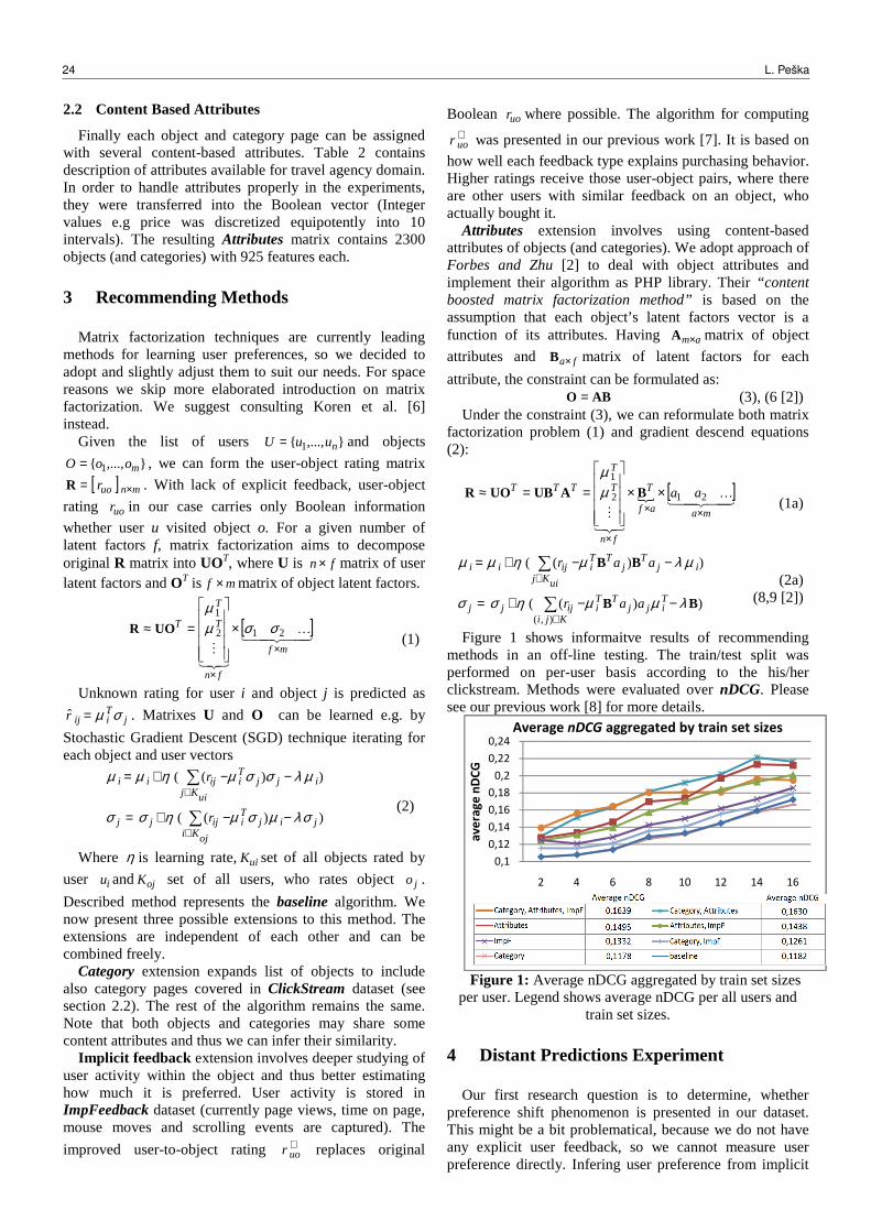
2.2 Content Based Attributes

Finally each object and category page can be assigned with several content-based attributes. Table 2 contains description of attributes available for travel agency domain. In order to handle attributes properly in the experiments, they were transferred into the Boolean vector (Integer values e.g price was discretized equipotently into 10 intervals). The resulting Attributes matrix contains 2300 objects (and categories) with 925 features each.

3 Recommending Methods

Matrix factorization techniques are currently leading methods for learning user preferences, so we decided to adopt and slightly adjust them to suit our needs. For space reasons we skip more elaborated introduction on matrix factorization. We suggest consulting Koren et al. [6] instead.

Given the list of users ,..., 1 nuuU = and objects

,..., 1 mooO = , we can form the user-object rating matrix

[ ] mnuor ×=R . With lack of explicit feedback, user-object

rating uor in our case carries only Boolean information

whether user u visited object o. For a given number of latent factors f, matrix factorization aims to decompose original R matrix into UOT, where U is fn× matrix of user latent factors and OT

is mf × matrix of object latent factors.

[ ]4434421K

321M mf

fn

T

T

T

×

×

×

=≈ 212

1

σσµµ

UOR

(1)

Unknown rating for user i and object j is predicted as

jTiijr σµ=ˆ . Matrixes U and O can be learned e.g. by

Stochastic Gradient Descent (SGD) technique iterating for each object and user vectors

))((

))((

jijTi

ojKiijjj

ijjTi

uiKjijii

r

r

σλµσµησσ

µλσσµηµµ

−−+=

−−+=

∑

∑

∈

∈ (2)

Where η is learning rate, uiK set of all objects rated by

user iu and ojK set of all users, who rates object jo .

Described method represents the baseline algorithm. We now present three possible extensions to this method. The extensions are independent of each other and can be combined freely.

Category extension expands list of objects to include also category pages covered in ClickStream dataset (see section 2.2). The rest of the algorithm remains the same. Note that both objects and categories may share some content attributes and thus we can infer their similarity.

Implicit feedback extension involves deeper studying of user activity within the object and thus better estimating how much it is preferred. User activity is stored in ImpFeedback dataset (currently page views, time on page, mouse moves and scrolling events are captured). The

improved user-to-object rating +uor replaces original

Boolean uor where possible. The algorithm for computing +uor was presented in our previous work [7]. It is based on

how well each feedback type explains purchasing behavior. Higher ratings receive those user-object pairs, where there are other users with similar feedback on an object, who actually bought it.

Attributes extension involves using content-based attributes of objects (and categories). We adopt approach of Forbes and Zhu [2] to deal with object attributes and implement their algorithm as PHP library. Their “content boosted matrix factorization method” is based on the assumption that each object’s latent factors vector is a function of its attributes. Having am×A matrix of object

attributes and fa×B matrix of latent factors for each

attribute, the constraint can be formulated as: ABO = (3), (6 [2])

Under the constraint (3), we can reformulate both matrix factorization problem (1) and gradient descend equations (2):

[ ]4434421K

321M maaf

T

fn

T

T

TTT aa

××

×

××

==≈ 212

1

BAUBUOR µµ

(1a)

))((

))((

),(

BB

BB

λµµησσ

µλµηµµ

−−+=

−−+=

∑

∑

∈

∈

Tijj

TTi

Kjiijjj

ijT

jTT

i

uiKjijii

aar

aar

(2a) (8,9 [2])

Figure 1 shows informaitve results of recommending methods in an off-line testing. The train/test split was performed on per-user basis according to the his/her clickstream. Methods were evaluated over nDCG. Please see our previous work [8] for more details.

Figure 1: Average nDCG aggregated by train set sizes

per user. Legend shows average nDCG per all users and train set sizes.

4 Distant Predictions Experiment

Our first research question is to determine, whether preference shift phenomenon is presented in our dataset. This might be a bit problematical, because we do not have any explicit user feedback, so we cannot measure user preference directly. Infering user preference from implicit

0,1

0,12

0,14

0,16

0,18

0,2

0,22

0,24

2 4 6 8 10 12 14 16

av

era

ge

nD

CG

Train set size per user

Average nDCG aggregated by train set sizes

24 L. Peška

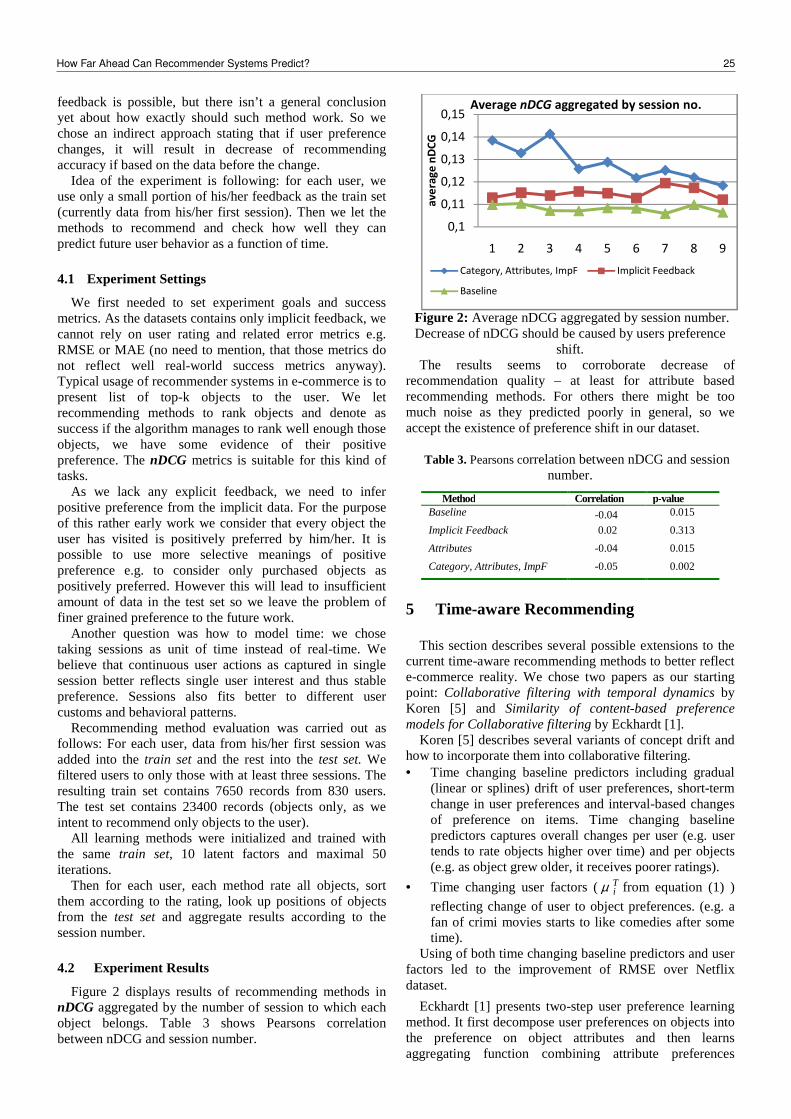
feedback is possible, but there isn’t a general conclusion yet about how exactly should such method work. So we chose an indirect approach stating that if user preference changes, it will result in decrease of recommending accuracy if based on the data before the change.

Idea of the experiment is following: for each user, we use only a small portion of his/her feedback as the train set (currently data from his/her first session). Then we let the methods to recommend and check how well they can predict future user behavior as a function of time.

4.1 Experiment Settings

We first needed to set experiment goals and success metrics. As the datasets contains only implicit feedback, we cannot rely on user rating and related error metrics e.g. RMSE or MAE (no need to mention, that those metrics do not reflect well real-world success metrics anyway). Typical usage of recommender systems in e-commerce is to present list of top-k objects to the user. We let recommending methods to rank objects and denote as success if the algorithm manages to rank well enough those objects, we have some evidence of their positive preference. The nDCG metrics is suitable for this kind of tasks.

As we lack any explicit feedback, we need to infer positive preference from the implicit data. For the purpose of this rather early work we consider that every object the user has visited is positively preferred by him/her. It is possible to use more selective meanings of positive preference e.g. to consider only purchased objects as positively preferred. However this will lead to insufficient amount of data in the test set so we leave the problem of finer grained preference to the future work.

Another question was how to model time: we chose taking sessions as unit of time instead of real-time. We believe that continuous user actions as captured in single session better reflects single user interest and thus stable preference. Sessions also fits better to different user customs and behavioral patterns.

Recommending method evaluation was carried out as follows: For each user, data from his/her first session was added into the train set and the rest into the test set. We filtered users to only those with at least three sessions. The resulting train set contains 7650 records from 830 users. The test set contains 23400 records (objects only, as we intent to recommend only objects to the user).

All learning methods were initialized and trained with the same train set, 10 latent factors and maximal 50 iterations.

Then for each user, each method rate all objects, sort them according to the rating, look up positions of objects from the test set and aggregate results according to the session number.

4.2 Experiment Results

Figure 2 displays results of recommending methods in nDCG aggregated by the number of session to which each object belongs. Table 3 shows Pearsons correlation between nDCG and session number.

Figure 2: Average nDCG aggregated by session number. Decrease of nDCG should be caused by users preference

shift. The results seems to corroborate decrease of

recommendation quality – at least for attribute based recommending methods. For others there might be too much noise as they predicted poorly in general, so we accept the existence of preference shift in our dataset.

Table 3. Pearsons correlation between nDCG and session

number.

Method Correlation p-value Baseline -0.04 0.015

Implicit Feedback 0.02 0.313

Attributes -0.04 0.015

Category, Attributes, ImpF -0.05 0.002

5 Time-aware Recommending

This section describes several possible extensions to the current time-aware recommending methods to better reflect e-commerce reality. We chose two papers as our starting point: Collaborative filtering with temporal dynamics by Koren [5] and Similarity of content-based preference models for Collaborative filtering by Eckhardt [1].

Koren [5] describes several variants of concept drift and how to incorporate them into collaborative filtering. • Time changing baseline predictors including gradual

(linear or splines) drift of user preferences, short-term change in user preferences and interval-based changes of preference on items. Time changing baseline predictors captures overall changes per user (e.g. user tends to rate objects higher over time) and per objects (e.g. as object grew older, it receives poorer ratings).

• Time changing user factors (Tiµ from equation (1) )

reflecting change of user to object preferences. (e.g. a fan of crimi movies starts to like comedies after some time).

Using of both time changing baseline predictors and user factors led to the improvement of RMSE over Netflix dataset.

Eckhardt [1] presents two-step user preference learning method. It first decompose user preferences on objects into the preference on object attributes and then learns aggregating function combining attribute preferences

0,1

0,11

0,12

0,13

0,14

0,15

1 2 3 4 5 6 7 8 9

av

era

ge

nD

CG

Average nDCG aggregated by session no.

Category, Attributes, ImpF Implicit Feedback

Baseline

How Far Ahead Can Recommender Systems Predict? 25

together. The benefits of this method is simple and direct way how to compute user preference for new or changed objects and compare users without common objects.

In the paper, standard collaborative filtering was applied with user similarity based on the two-step method and successfully tested on the Netflix dataset with RMSE measure.

There are several important differences between Netflix and E-Commerce use-cases: possibility of extracting object attributes can significantly improve our prospect in capturing long-term user preferences. Also recording user actions might be usefull.

1. Some of the object attributes, let us call them the “soft attributes” are changeable over time. The most important one are probably prices and discounts, but there are also others depending on the domain (e.g. warranty, stock availability, range of services, promotions etc.).

2. Ordered attributes should be considered according to the context of available objects at the time being, especially at fast evolving domains e.g. computers, cellphones, cars etc. This might help us in capturing long-term preferences: attributes of high-end computer became average within a year, but the user will probably still prefer high-end computers.

3. Last but not least, due to rather complex monitoring of user behavior, we might be able to infer user actions leading to preference shift (purchase action is a good candidate) and/or periodical behavior.

We plan to adjust Koren’s model to incorporate attributes and treat them relatively with respect to their current range. The changes of the object’s attributes can be recorded, so we can restore their values at any time-point, however the question is how to model the same object with different attributes at different time-points.

Eckhards method provides simple way how to compute user preference for any set of attribute values, so we plan to experiment with changing users previous ratings as results of users or objects actions.

6 Conclusions

In this paper we focused on recommending for e-commerce portals. We were particularly interested in time-aware recommending. We described problems and constraints of e-commerce domain and presented methods capable to deal with them.

An off-line experiment corroborated negative dependence of increasing time-distance between training and recommending on the quality of recommendations (measured by nDCG) and thus need of time-aware methods. We concluded the paper with several proposals on adjusting contemporary recommending methods to better reflect time-drifting nature of e-commerce datasets.

Acknowledgment

The work on this paper was supported by the grant SVV-2013-267312, GAUK-126313 and P46.

References

[1] Eckhardt, A. Similarity of users (content-based) preference models for Collaborative filtering in few ratings scenário. EXPERT SYST APPL, 2012, 39, 11511 - 11516

[2] Forbes, P. & Zhu, M. Content-boosted matrix factorization for recommender systems: experiments with recipe recommendation. In RecSys 2011, ACM, 2011, 261-264

[3] Ito, F.; Hiroyasu, T.; Miki, M.; Yokouchi, H.; Detection of preference shift timing using time-series clustering, In FUZZ-IEEE 2009, IEEE, 2009, 1585 - 1590

[4] Konstan, J. & Riedl, J. Recommender systems: from algorithms to user experience. UMUAI, 2012, 22, 101-123.

[5] Koren, Y. Collaborative filtering with temporal dynamics. In ACM SIGKDD 2009, ACM, 2009, 447-456.

[6] Koren, Y.; Bell, R. & Volinsky, C. Matrix Factorization Techniques for Recommender Systems. Computer, IEEE, 2009, 42, 30-37.

[7] Peska, L.; Vojtas, P.: Negative Implicit feedback in E-commerce Recommender Systems. In WIMS 2013, ACM, 2013, 45:1 – 45:4

[8] Peska, L.; Vojtas, P Recommending for Disloyal Customers with Low Consumption Rate. In review for RecSys 2013, http://www.ksi.mff.cuni.cz/~peska/recsys2013.pdf

[9] Takahashi M., Nakao T., Tsuda K. and Terano T. Generating Dual-Directed Recommendation Information from Point-of-Sales Data of a Supermarket, In KES 2008, Springer, 2008, 1010 - 1017

26 L. Peška

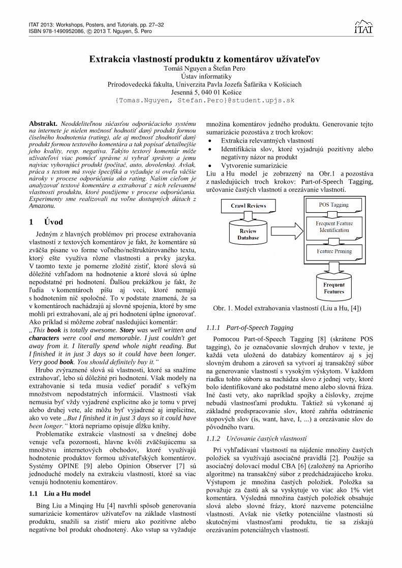
Extrakcia vlastností produktu z komentárov užívateľov

Tomáš Nguyen a Štefan Pero

Ústav informatiky

Prírodovedecká fakulta, Univerzita Pavla Jozefa Šafárika v Košiciach

Jesenná 5, 040 01 Košice Tomas.Nguyen, Stefan.Pero@student.upjs.sk

Abstrakt. Neoddeliteľnou súčasťou odporúčacieho systému na internete je nielen možnosť hodnotiť daný produkt formou číselného hodnotenia (rating), ale aj možnosť zhodnotiť daný produkt formou textového komentára a tak popísať detailnejšie jeho kvality, resp. negatíva. Takýto textový komentár môže užívateľovi viac pomôcť správne si vybrať správny a jemu najviac vyhovujúci produkt (počítač, auto, dovolenku). Avšak, práca s textom má svoje špecifiká a vyžaduje si oveľa väčšie nároky v procese odporúčania ako rating. Našim cieľom je analyzovať textové komentáre a extrahovať z nich relevantné vlastnosti produktu, ktoré použijeme v procese odporúčania. Experimenty sme realizovali na voľne dostupných dátach z Amazonu.

1 Úvod

Jedným z hlavných problémov pri procese extrahovania

vlastností z textových komentárov je fakt, že komentáre sú

zväčša písane vo forme voľného/neštruktúrovaného textu,

ktorý ešte využíva rôzne vlastnosti a prvky jazyka.

V taomto texte je pomerne zložité zistiť, ktoré slová sú

dôležité vzhľadom na hodnotenie a ktoré slová sú úplne

nepodstatné pri hodnotení. Ďalšou prekážkou je fakt, že

ľudia v komentároch píšu aj veci, ktoré nemajú

s hodnotením nič spoločné. To v podstate znamená, že sa

v komentároch nachádzajú aj slovné spojenia, ktoré by sme

mohli pri extrahovaní, ale aj pri hodnotení úplne ignorovať.

Ako príklad si môžeme zobrať nasledujúci komentár:

„This book is totally awesome. Story was well written and

characters were cool and memorable. I just couldn't get

away from it. I literally spend whole night reading. But

I finished it in just 3 days so it could have been longer.

Very good book. You should definitely buy it.“

Hrubo zvýraznené slová sú vlastnosti, ktoré sa snažíme

extrahovať, lebo sú dôležité pri hodnotení. Však modely na

extrahovanie si teda musia vedieť poradiť s veľkým

množstvom nepodstatných informácií. Vlastnosti však

nemusia byť vždy vyjadrené explicitne ako je tomu v prvej

alebo druhej vete, ale môžu byť vyjadrené aj implicitne,

ako vo vete „But I finished it in just 3 days so it could have

been longer.“ ktorá nepriamo opisuje dĺžku knihy.

Problematike extrakcie vlastností sa v dnešnej dobe

venuje veľa pozornosti, hlavne kvôli zväčšujúcemu sa

množstvu internetových obchodov, ktoré využívajú

hodnotenie produktov formou užívateľských komentárov.

Systémy OPINE [9] alebo Opinion Observer [7] sú

jednoduché modely na extrakciu vlastností, ktoré sa viac

venujú hodnoteniu komentárov.

1.1 Liu a Hu model

Bing Liu a Minqing Hu [4] navrhli spôsob generovania

sumarizácie komentárov užívateľov na základe vlastností

produktu, snažili sa zistiť mieru ako pozitívne alebo

negatívne bol produkt ohodnotený. Ako vstup sa vyžaduje

množina komentárov jedného produktu. Generovanie tejto

sumarizácie pozostáva z troch krokov:

Extrakcia relevantných vlastností

Identifikácia slov, ktoré vyjadrujú pozitívny alebo

negatívny názor na produkt

Vytvorenie sumarizácie

Liu a Hu model je zobrazený na Obr.1 a pozostáva

z nasledujúcich troch krokov: Part-of-Speech Tagging,

určovanie častých vlastnotí a orezávanie vlastnotí.

Obr. 1. Model extrahovania vlastností (Liu a Hu, [4])

1.1.1 Part-of-Speech Tagging

Pomocou Part-of-Speech Tagging [8] (skrátene POS

tagging), čo je označovanie slovných druhov v texte, je

každá veta uložená do databázy komentárov aj s jej

slovným druhom a zároveň sa vytvorí aj transakčný súbor

na generovanie vlastností s vysokým výskytom. V každom

riadku tohto súboru sa nachádza slovo z jednej vety, ktoré

bolo identifikované ako podstatné meno alebo slovná fráza.

Iné časti vety, ako napríklad spojky a číslovky, zrejme

nebudú vlastnosťami produktu. Taktiež sú vykonané aj

základné predspracovanie slov, ktoré zahŕňa odstránenie

stopových slov (is, want, have, I, ...) a orezávanie slov do

pôvodného tvaru.

1.1.2 Určovanie častých vlastností

Pri vyhľadávaní vlastností na nájdenie množiny častých

položiek sa využívajú asociačné pravidlá [2]. Použije sa

asociačný dolovací modul CBA [6] (založený na Aprioriho

algoritme) na transakčný súbor z predchádzajúceho kroku.

Výstupom je množina častých položiek. Položka sa

považuje za častú ak sa vyskytuje vo viac ako 1% viet

komentára. Výsledná množina častých položiek obsahuje

slová alebo slovné frázy, ktoré nazveme potenciálne

vlastnosti. Avšak nie všetky potenciálne vlastnosti sú

skutočnými vlastnosťami produktu, tie sa získajú

orezávaním potenciálnych vlastností.

ITAT 2013: Workshops, Posters, and Tutorials, pp. 27–32ISBN 978-1490952086, c© 2013 T. Nguyen, Š. Pero

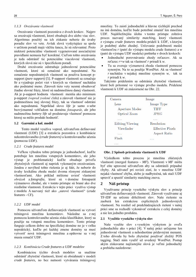
1.1.3 Orezávanie vlastností

Orezávanie vlastností pozostáva z dvoch krokov. Najprv

sa orezávajú vlastnosti, ktoré obsahujú dve alebo viac slov.

Algoritmus použitý na ich získanie neberie do úvahy

poradie slov vo vete. Avšak slová vyskytujúce sa spolu

v určitom poradí majú väčšiu šancu, že sú relevantné. Preto

niektoré potenciálne vlastnosti vygenerované asociačnými

pravidlami nemusia byť korektné. Cieľom tohto orezávania

je teda odstrániť tie potenciálne viacslovné vlastnosti,

ktorých slová nie sú v špecifickom poradí.

Druhé orezávanie odstraňuje jednoslovné potenciálne

vlastnosti, ktoré sú označené ako nepodstatné. Na

označenie nepodstatných vlastností sa používa koncept p-

support (pure support) [5]. P-support vlastnosti sa označuje

ftr a vyjadruje počet viet v ktorých sa vlastnosť nachádza

ako podstatné meno. Zároveň tieto vety nesmú obsahovať

žiadne slovné frázy, ktoré sú nadmnožinou danej vlastnosti.

Ak je p-support hodnota vlastnosti menšia ako minimum

p-support (vopred zvolené číslo) a zároveň vlastnosť nie je

podmnožinou inej slovnej frázy, tak sa vlastnosť odstráni

ako nepodstatná. Napríklad slovo life je samo o sebe

bezvýznamné vzhľadom na doménu fotoaparát, ale jeho

nadmnožina battery life už predstavuje vlastnosť pomocou

ktorej sa môže produkt hodnotiť.

1.2 Garenini a kol. model

Tento model využíva vopred, užívateľom definované

vlastnosti (UDF) [3] a extrakcia pozostáva z kombinácie

nekontrolovaného (crude features) a kontrolovaného učenia

(pomocou UDF).

1.2.1 Crude features model

Veľkou výhodou tohto prístupu je jednoduchosť, keďže

potrebuje len množinu vstupných komentárov, ale jeho

výstup je problematický keďže obsahuje priveľa

zbytočných vlastností aj napriek vykonaným orezávaniam.

Jendou z nevýhod tohto riešenia je aj fakt, že neberie do

úvahy lexikálnu zhodu medzi dvoma rôznymi získanými

vlastnosťami. Ako príklad môžeme uviesť vlastnosti

obrázok a fotografia, ktoré sú v doméne fotoaparát

významovo zhodné, ale v tomto prístupe sú brané ako dve

rozdielne vlastnosti. Extrakcia v tejto práci využíva výstup

z modelu A nazvaný tiež ako „surové vlastnosti“ (crude

features - CF).

1.2.2 UDF model

Pomocou užívateľom definovaných vlastností sa vytvorí

tréningová množina komentárov. Následne sa z nej

pomocou kontrolovaného učenia získa klasifikátor, ktorý sa

použije na vstupnú množinu komentárov. Tento prístup

funguje celkom dobre na špecifickej doméne no je v celku

nepraktický, keďže pri každej zmene domény sa musí

vytvoriť nová tréningová množina a opätovne sa v nej

musia označiť UDF.

1.2.3 Kombinácia Crude features a UDF modelov

Kombináciou týchto dvoch modelov sa snažíme

odstrániť zbytočné vlastnosti, ktoré sú obsiahnuté v modeli

crude features, no bez nutnosti vytvárania tréningovej

množiny. To zaistí jednoduchší a hlavne rýchlejší prechod

na inú doménu, keďže bude potrebné zmeniť len množinu

UDF. Najdôležitejšiu úlohu v tomto prístupe zohráva

proces nazvaný similarity matching, ktorý vlastnosti

z výstupu crude features modelu pridelí k UDF, s ktorým

je podobný alebo zhodný. Určovanie podobnosti medzi

vlastnosťou r (patrí do výstupu modelu crude features) a w

(patrí do výstupu UDF modelu) prebieha v dvoch krokoch:

Jednoduché porovnávanie zhody reťazcov. Ak sa

reťazec r=w tak sa vlastnosť r priradí k w.

Tu sa overuje významová zhoda vlastností pomocou

synoným. Na to sa použije WordNet. Ak sa vlastnosť

r nachádza v nejakej množine synoným w, tak sa

r priradí k w.

Takýmto pridelením sa odstránia zbytočné vlastnosti,

ktoré boli prítomné vo výstupe prvého modelu. Pridelené

vlastnosti k UDF sú znázornené na Obr. 22.

Obr. 2 Spôsob priradenia vlastností k UDF

Výsledkom tohto procesu je množina zlúčených

vlastností (merged features - MF). Vlastnosti v MF môžu

byť ešte upravené užívateľom aby sa odstránili prípadné

chyby. Ak užívateľ pri revízii zistí, že v množine UDF

nejaká vlastnosť chýba, alebo je nadbytočná, tak stačí UDF

upraviť a spustiť similarity matching znova.

2 Náš prístup

Využívame princíp vysokého výskytu slov a princíp

užívateľom definovaných vlastností. Zároveň využívame aj

TF-IDF na určenie dôležitosti slov. Naše riešenie sa

zaoberá len extrakciou explicitných jednoslovných

vlastností. Na rozdiel od predchádzajúcich riešení v našej

práci sme sa rozhodli vykonávať extrakciu z celej domény

a nie len jedného produktu.

2.1 Využitie vysokého výskytu slov

Naše využite slov s vysokým výskytom je oveľa

jednoduchšie ako v práci [4]. V našej práci určujeme len

jednoslovné vlastnosti a nehodnotíme prídavnými menami.

Z toho dôvodu by bolo zbytočné používať zložitý POS

tagging. Stačí nám využiť už uvedený WordNet. Postup

akým získavame najčastejšie slová je veľmi jednoduchý

a prebieha nasledovne:

28 T. Nguyen, Š. Pero

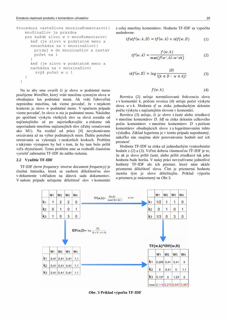
Procedura casteSlova mnozinaKomentarov)

množinaSlov je prázdna

pre každé slovo w v mnozKomentarov

keď (je slovo w podstatné meno a

nenachádza sa v mnozinaSlov)

pridaj w do mnozinaSlov a nastav

počet na 1

keď (je slovo w podstatné meno a

nachádza sa v mnozinaSlov)

zvýš počet w o 1

Na to aby sme overili či je slovo w podstatné meno

použijeme WordNet, ktorý vráti množinu synoným slova w

obsahujúce len podstatné mená. Ak vráti ľubovoľnú

neprázdnu množinu, tak vieme povedať, že v nejakom

kontexte je slovo w podstatné meno. V opačnom prípade

vieme povedať, že slovo w nie je podstatné meno. Následne

po spočítaní výskytu všetkých slov sa slová zoradia od

najčastejšieho až po najzriedkavejšie a získame tak

usporiadanú množinu najčastejších slov (ďalej označovanú

ako M1). Na rozdiel od práce [4] nevykonávame

orezávania až na výber podstatných mien. Ďalšie potrebné

orezávania sa vykonajú v neskorších krokoch. Problém

s takýmto výstupom by bol v tom, že by tam bolo príliš

veľa zbytočností. Tento problém sme sa rozhodli čiastočne

vyriešiť zahrnutím TF-IDF do nášho riešenia.

2.2 Využitie TF-IDF

TF-IDF (term frequency–inverse document frequency) je

číselná štatistika, ktorá sa zaoberá dôležitosťou slov

v dokumente vzhľadom na dátovú sadu dokumentov.

V našom prípade určujeme dôležitosť slov v komentári

z celej množiny komentárov. Hodnota TF-IDF sa vypočíta

nasledovne:

(1)

(2)

(3)

(4)

Rovnica (2) určuje normalizovanú frekvenciu slova

s v komentári k, pričom rovnica (4) určuje počet výskytu

slova w v k. Hodnota tf sa získa jednoduchým delením

počtu výskytu s najčastejším slovom v komentári.

Rovnica (3) určuje, či je slovo s časté alebo zriedkavé

v množine komentárov D. Idf sa získa delením celkového

počtu komentárov v množine komentárov D s počtom

komentárov obsahujúcich slovo s a logaritmovaním tohto

výsledku. Základ logaritmu je v tomto prípade nepodstatný,

nakoľko nás zaujíma skôr porovnávanie hodnôt než ich

presnosť.

Hodnota TF-IDF sa získa už jednoduchým vynásobením

hodnôt z (2) a (3). Veľmi dobrou vlastnosťou TF-IDF je to,

že ak je slovo príliš časté, alebo príliš zriedkavé tak jeho

hodnota bude horšia. V našej práci nevyužívame jednotlivé

hodnoty TF-IDF ale ich priemer, ktorý nám ukáže

priemernú dôležitosť slova. Čím je priemerná hodnota

menšia tým je slovo dôležitejšie. Príklad výpočtu

a priemeru je znázornený na Obr.3.

Obr. 3 Príklad výpočtu TF-IDF

Extrakcia vlastností produktu z komentárov užívatel’ov 29

V pravom hornom rohu je tabuľka výskytu slov w1, w2,

w3, w4 v komentároch k1, k2, k3. Pomocou rovníc (2) a (3)

vytvoríme dve rôzne tabuľky uchovávajúce hodnoty tf a idf.

Následne hodnoty v tabuľke vynásobíme z čoho nám

vznikne tabuľka obsahujúca hodnoty TF-IDF. Nakoniec z

hodnôt všetkých slov vypočítame priemer, ktorý je na Obr.

v štvrtom riadku. Slovo w3 ktoré je veľmi bežné a slovo

w4, ktoré je veľmi zriedkavé majú najväčšiu priemernú

hodnotu a tým pádom ich nebudeme považovať za dôležité.

Keďže slová w1 a w2 majú priemernú najmenšiu hodnotu,

tak ich považujeme za dôležité. Je dôležité dodať, že nás

nezaujíma konkrétna hodnota priemerov, ale skôr len

niekoľko najmenších hodnôt, ktoré budeme považovať za

potenciálne vlastnosti. Tak ako aj v predchádzajúcom

kroku aj tu využívame WordNet na výber len podstatných

mien. Tento výber sa však deje až po vyrátaní TF-IDF

priemerov.

Z tohto kroku dostaneme zoznam podstatných mien s ich

priemernou TF-IDF hodnotou, ktorý následne usporiadame

od slov s najmenšou hodnotou až po tie s najväčšou.

Výsledkom bude usporiadaná množina najdôležitejších

slov (ďalej označovanú ako M2). V ďalšom kroku budeme

využívať nielen tento, ale predošlý usporiadaný zoznam.

2.3 Určovanie relevantných vlastností

Pri určovaní relevantných vlastností využívame aj

užívateľom definované vlastnosti. Naše využitie UDF je

podobné prístupu opísanom v podkapitole 1.2.2. Vopred si

zadáme množinu slov, ktoré budú predstavovať množinu

UDF pre danú doménu, v našom prípade knihy, filmy a

hudba.

2.3.1 Similarity matching

Vstupom pre similarity matching sú usporiadané

množiny najčastejších a najdôležitejších slov (množiny M1

a M2), ktoré tvoria naše potenciálne vlastnosti.

Priradzovanie slov k UDF prebieha tak, že si všetky

slová z usporiadanej množiny najčastejších alebo

najdôležitejších slov porovnávame so slovami v UDF.

Výsledkom je množina zlúčených vlastností (množina MF).

Tento výstup je však oveľa jednoduchší ako

predchádzajúci, keďže obsahuje len riadky v ktorých je

potenciálna vlastnosť s UDF vlastnosťou.

2.3.2 Zoznam výskytu slov

V tomto kroku využijeme ako vstup množiny M1, M2

a MF získané z predošlých krokov. Zvolíme číslo x, ktoré

bude predstavovať počet prvých slov z celkového počtu

slov z množiny M1 a číslo y, ktoré bude predstavovať počet

prvých slov z celkového počtu slov z množiny M2 .

Cieľom tohto kroku je vytvorenie zoznamu výskytu

jednotlivých slov. Tento zoznam obsahuje slová, ktoré sa

nachádzajú medzi najčastejšími slovami (prvých x % slov),

medzi najdôležitejšími slovami (prvých y % slov) a ďalej či

sa slovo nachádza v množine MF, t.j. či je to slovo

podobné s nejakým slovom z UDF. Príklad výskytu slova

vyzerá nasledovne:

book 0 1 1

Slovo book sa nevyskytuje v najčastejších slovách (0),

nachádza sa v najdôležitejších slovách (1) a vyskytuje sa v

množine MF (1).

2.3.3 Hodnotenie slov

Hodnotenie slov prebieha nasledovne: pre každé slovo v zozname výskytov

ak je výskyt typu 100 alebo 010 tak

slovu priradíme index α

ak je výskyt typu 110 tak slovu

priradíme index β

ak je výskyt typu 101 alebo 011 tak

slovu priradíme index γ

ak je výskyt typu 111 tak dáme slovu

priradíme index δ

Pre každý model vopred nastavíme jeho dôležitosť pri

súhrnom vyhľadávaní vlastností, napríklad tieto štyri

indexy si môžeme zvoliť nasledovne: α - 0.0; β - 0.5; γ -

1.0; δ - 2.0. Tieto konkrétne hodnotenia sme si zvolili

hlavne pre jednoduchšiu vizuálnu a číselnú reprezentáciu.

Dôvody jednotlivých ohodnotení sú nasledovné:

Ak sa slovo nachádza len v jednej množín M1 alebo M2

a zároveň sa nenachádza ani v množine MF, tak slovo má

len malú šancu byť relevantnou vlastnosťou. Preto dostáva

hodnotenie 0.0.

Ak sa slovo nachádza v oboch množinách M1 a M2, ale

sa nenachádza v množine MF, tak dostanie hodnotenie 0.5.

Dôvodom tohto hodnotenia je to, že slovo sa nenachádza

v MF, preto ho nebudeme považovať za relevantnú

vlastnosť. Zároveň sa však nachádza v M1 a M2 a tým

pádom tu je možnosť, že slovo je vlastnosťou ale jeho

synonymum nie je v množine UDF.

Ak sa slovo nachádza v jednej z množín M1 alebo M2

a zároveň v množine MF, tak slovo dostane hodnotenie 1.0.

V tomto prípade je slovo označené ako najdôležitejšie,

alebo najčastejšie a je podobné/zhodné s nejakým slovom

z UDF. Preto ho budeme považovať za relevantnú

vlastnosť.

Ak sa slovo nachádza v oboch množinách M1 a M2

a zároveň sa nachádza v množine MF, tak dostane

hodnotenie 2.0. Takéto slovo budeme považovať za

relevantnú vlastnosť, lebo je označené ako dôležité aj časté

a je podobné s nejakým slovom z množiny UDF.

Výstup bude obsahovať vlastnosti ku ktorým je pridelené

hodnotenie. Následne vyberieme len tie s hodnotením 1.0

alebo 2.0 ako relevantné. Vlastnosti s hodnotením 0.5

môžeme použiť na overenie korektnosti našej UDF

množiny. Ak sa medzi týmito slovami nachádza nejaké

slovo pri ktorom sme si istý, že je vlastnosťou, tak ho

(alebo jeho synonymum) pridáme do UDF.

3 Experimenty

3.1 Dátová sada

UDF množina z domény knihy, filmy a hudba obsahuje

vlastnosti (napr. book, film, story, music, length, character,

album, lyrics) získané pomocou doménového expert z

IMDB.com.

30 T. Nguyen, Š. Pero

Naša dátová sada obsahuje vyše päť miliónov

komentárov z AMAZON.com. Dáta obsahujú informácie o

produkte, jeho hodnotenie a textový komentár. Používali

sme túto dátovú sadu v štyroch veľkostiach (Tab. 1).

Tab 1. Veľkosti dátových sád

Sada Počet komentárov

Sada1 50 000

Sada2 100 000

Sada3 250 000

Sada4 400 000

3.2 Výsledky testovania na celej doméne

V prvom teste sme sa rozhodli zobrať pri hodnotení prvých

5% najčastejších slov (množina M1) a prvých 20%

najdôležitejších slov (množina M2). Pozorovaním dát sme

zistili, že relevantné vlastnosti v množine M2 sa nachádzajú

oveľa „hlbšie“ v zozname ako v M1 a z toho dôvodu

berieme viac slov z M2 ako z M1. Výsledky sú zobrazené v

Tab.2. Ako výsledné vlastnosti sme zobrali tie

s hodnotením väčším alebo rovným ako 1.0. Pri dátovej

sade 1 môžeme vidieť iba štyri slová s hodnotením 2.0

pričom pri väčších vzorkách je ich viac. To je spôsobené

hlavne veľkosťou prvej vzorky. Ďalej sme si všimli, že so

zväčšujúcou sa vzorkou sa nezväčšuje počet nových slov

s priaznivým hodnotením. Tento fakt nám ukazuje to, že

keď sa zväčšuje vzorka tak sa pozícia najčastejších

a najdôležitejších slov výrazne nezhoršuje a tým pádom sú

tieto slová pravdepodobnejšími vlastnosťami. Keď sa ale

pozrieme bližšie na niektoré slová, tak nájdeme také, ktoré

nám nepripadajú ako relevantné vlastnosti v našej doméne.

Sú to slová ako napríklad: account alebo history. Hlavne

slovo history sa objavuje vo väčších vzorkách

s hodnotením 2.0 čo znamená že je medzi prvou tisíckou

najčastejších ale aj najdôležitejších slov. No táto vlastnosť

nie je relevantná v našej doméne. Dôvodov môže byť hneď

niekoľko.

Prvým z možných dôvodov je rozmanitosť našej vzorky,

nakoľko pracujeme až na troch doménach súčasne, pričom

modely na ktoré sme nadväzovali sa zaoberali extrakciou

len z množiny komentárov jedného produktu.

Ďalším z možných dôvodov môže byť veľké striedanie

rôznych produktov v našich vzorkách. Opätovne problém

s viacerými produktmi spracovanými zároveň. Aby sme si

naše predpoklady overili vykonali sme testovanie na vzorke

obsahujúcej len komentáre pre jeden produkt.

3.3 Výsledky testovania pre jeden produkt

Pre tento test sme vytvorili testovacie vzorky, ktoré

obsahovali komentáre o jednom filme (príklad Sada5 a

Sada6). Kedže sme testovaciu doménu zúžili na filmy, tak

sme tomu museli prispôsobiť našu množinu UDF.

V tomto prípade sme takisto zobrali prvých 5% slov

z množiny M1 a prvých 20% slov z množiny M2 v oboch

dátových sadách. Ohodnotené vlastnosti sú zobrazené v

Tab.3.

Tab. 3 Ohodnotené vlastnosti pre jeden produkt

Sada 5 Sada 6

1.0 2.0 1.0 2.0

movie film part film

story length movie

part cinema story

length

cinema

case

Tab. 2 Ohodnotené vlastnosti testovacích vzoriek

Sada1 Sada2 Sada3 Sada4

1.0 2.0 1.0 2.0 1.0 2.0 1.0 2.0

album book album book album book album book

movie story movie story movie story movie story

film part film part film part film part

music charact

er music charact

er music charact

er music charact

er history quality history quality history quality history

quality role case words case role case

case words picture role words

role picture record picture

words record level record

picture level tale level

record tale type tale

level type volume type

tale volume langua

ge volume

Extrakcia vlastností produktu z komentárov užívatel’ov 31

Pozorovaním týchto výsledkov sme prišli na to, že

väčšina slov s ohodnotením 1.0 aj 2.0 môžu byť

považované za relevantné v oboch dátových sadách. Tiež si

môžeme všimnúť zlepšenie hodnotenia vlastností movie

a story v dátovej sade 6, v ktorej sa už nevyskytuje

vlastnosť case, ktorá nebola vzhľadom na našu doménu

relevantná.

Oproti testovaniu na celej doméne tu značne poklesol

počet diskutabilných vlastností. Zvýšila sa taktiež presnosť

extrahovaných vlastností. Tieto výsledky taktiež podporujú

naše predchádzajúce predpoklady, že s rozširujúcou sa

doménou a rôznorodosťou produktov sa výsledky

skresľujú.

Záver

Cieľom tejto práce bolo navrhnúť model na extrakciu

vlastností produktov z komentárov užívateľov. Navrhli sme

vlastné riešenie, ktoré nadväzovalo na existujúce riešenia v

tejto problematike, napr. číselnú štatistiku TF-IDF, ktorá

určuje dôležitosť slov v komentári na základe ich výskytu.

Následne sme na našej vzorke komentárov vykonali

potrebné testy na overenie funkcionality nášho riešenia.

Vzorka bola širšieho charakteru keďže obsahovala

komentáre produktov rôznych domén. Tieto testy ukázali,

že naše riešenie úspešne extrahuje vlastnosti

produktov z väčších domén. Testami sme však zistili aj to,

že presnosť extrakcie sa znižuje na dátových sadách, ktoré

obsahujú viacero domén a naopak presnosť je veľmi dobrá

ak vzorka obsahuje komentáre len z jednej domény.

V našej práci sme sa zaoberali extrakciou vlastností

produktov za účelom hodnotenia týchto produktov, ale naše

riešenie sa dá použiť aj na iné účely ako sú napríklad

odporúčacie systémy produktov. Takéto systémy sa

pokúšajú odhadnúť, aké položky by užívateľa zaujímali na

základe dostupných informácii o zákazníkovi a produktoch

[1].

V budúcich prácach môžeme nadviazať na túto prácu

s tým, že by sme aj hodnotili produkty pomocou

prídavných mien. Taktiež by sme doplnili extrakciu menej

častých vlastností a podobne.

Poďakovanie

Táto práca bola podporená v rámci výskumných

projektov VEGA 1/0832/12 a VVGS-PF-2013-102.

Referencie

[1] Aciar, Silvana, Debbie Zhang, Simeon Simoff a John

Debenham. Informed Recommender: Basing

Recommendations on Consumer Product Reviews.

IEEE Intelligent Systems. roč. 22, č. 3, s. 39-47. ISSN

1541-1672. DOI: 10.1109/MIS.2007.55

[2] Agrawal, Rakesh a Ramakrishnan Srikant. 20th

VLDB Conference: September 12 -15, 1994, Santiago

- Chile : proceedings of the 20th International

Conference on Very Large Data Bases. San Francisco:

Morgan Kaufmann Publishers, 1994, s. 487-499.

ISBN 1558601538.

[3] Carenni, Giuseppe, Raymond T. NG a Ed Zwart.

Proceedings of the Third International Conference on

Knowledge Capture: K-CAP '05 : October 2-5, 2005,

Banff, Alberta, Canada. New York, N.Y.: Association

for Computing Machinery, c2005, s. 11-18. ISBN 1-

59593-163-5.

[4] Hu, Minqing a Bing Liu. Mining and summarizing

customer reviews. Proceedings of the 2004 ACM

SIGKDD international conference on Knowledge

discovery and data mining - KDD '04. New York,

New York, USA: ACM Press, 2004, s. 168-177. DOI:

10.1145/1014052.1014073.

[5] Hu, Minqing a Bing Liu. Proceedings: Nineteenth

National Conference on Artificial Intelligence (AAAI-

04) : Sixteenth Innovative Applications of Artificial

Intelligence Conference (IAAI-04). Cambridge,

Mass.: MIT Press, c2004, s. 755-760. ISBN 0-262-

51183-5.

[6] Hu, Minqing a Bing Liu. Proceedings. Menlo Park,

Calif.: AAAI Press, c1998, s. 80-86. ISBN 1-57735-

070-7.

[7] Liu, Bing, Minqing Hu a Junsheng Cheng. Opinion

observer. Proceedings of the 14th international

conference on World Wide Web - WWW '05. New

York, New York, USA: ACM Press, 2005, s. 342-

351. DOI: 10.1145/1060745.1060797.

[8] Manning, Christopher D. Foundations of statistical

natural language processing. Cambridge: MIT Press,

c1999, xxxvii, 680 s. ISBN 02-621-3360-1.

[9] Popescu, Ana-Maria a Oren Etyioni. Extracting

product features and opinions from reviews.

Proceedings of the conference on Human Language

Technology and Empirical Methods in Natural

Language Processing - HLT '05. Morristown, NJ,

USA: Association for Computational Linguistics,

2005, s. 339-346. DOI: 10.3115/1220575.1220618

32 T. Nguyen, Š. Pero

Workshop on Bioinformatics in Genomicsand Proteomics

At the beginning of the year 2013 I was asked by Tomas Vinar and other organizers of ITAT to helporganize a bioinformatics workshop at this year’s conference. Organizing such workshop at ITATwas seen as a way to bridge the slowly narrowing gap and ease the relative isolation of the Czechand Slovak IT and molecular biology communities. The arrival of high-throughput techniques ofgenomics and proteomics to our laboratories in the last few years has increased the pressure onusing state of the art bioinformatics to crunch the ever increasing mountain of data. What used tobe single-gene or single-protein studies a few years ago is now being studied in a whole-genomeor whole-proteome context. I selected the workshop focus and title to specifically attract papersfrom the the area of big-data studies. However, being a first attempt of this kind, we also tried tokeep the workshop open to as many interested participants as possible. We therefore encouragedcontributions from systems biology, medical bioinformatics and other closely related disciplines.

The cross-disciplinary workshop setting partly reflects the dual reality of bioinformatics teach-ing and research at Czech and Slovak universities. On one hand, bioinformatics is firmly rooted innatural science curricula, either independently as is the case of the Faculty of Science of MasarykUniversity in Brno and the Faculty of Science of the South Bohemian University in Ceske Bude-jovice, or even hidden in courses, such as “Protein structure and function”, “Genome evolution”,etc. On the other hand, we also see bachelor and master programs in bioinformatics created asextensions of teaching computer science. This is the case of the bioinformatics programs at theFaculty of Informatics at Masaryk University in Brno and Faculty of Electrical Engineering andCommunication at the Brno University of Technology. It is also present in the curricula of theFaculty of Mathematics, Physics and Computer Science of the Comenius University in Bratislava,Faculty of Electrical Engineering of the Czech Technical University in Prague and Faculty of Chem-ical Technology of the Institute of Chemical Technology in Prague.

Although this workshop is one of the first bioinformatics workshops organized in the contextof a computer science conference, there is now quite a history of Czech and Slovak bioinformat-ics conferences and workshops that shared the same organizers or participants, or both. Thisincludes a series of conferences called Bioinformatics I, II and III organized during the INVEX fairin Brno by Dr. Jiri Damborsky in the years 2004-2006. The most prominent series of meetingsis beyond doubt the FOBIA annual or biannual meeting of Czech and Slovak bioinformatics com-munities taking place at various locations from the year 2004, first organized by Dr. Jan Paces(http://fobia.img.cas.cz/). I had the honor to organize the next meeting in Telc in 2005. The lastmeeting was the ENBIK conference in Cesky Sternberk in 2012 organized by Dr. Daniel Svozil.A series of summer schools in bioinformatics has been repeatedly organized by Dr. Tomas Vinarand Dr. Brona Brejova in Slovakia since the year 2007.

To underline the planned focus of the workshop on problems in genomics and proteomics, Iinvited Dr. Eduard Kejnovsky from the Institute of Biophysics of the Czech Academy of Sciences

33

to provide us with an introduction to the area of studying genomes. He kindly accepted theinvitiation. His lecture titled “Jumping genes – parasites or helpers?” should bring home the ideathat genomes are not static objects, but rather living systems in their own merit and that anyobservations we make are only snapshots of a highly dynamic system.

This workshop has attracted a modest number of papers from authors from Bratislava, Brno,Košice and Prague, with co-authors also from institutions in Canada and Mexico. The paperscover the areas of RNA structure analysis and prediction (Budis and Brejova, Rampasek et al.,Simalova), DNA sequence analysis (Brazdova et al.), genome-wide association studies (Stefanicand Lexa), pathway and expression analysis (Andel et al., Ihnatova), plant genome analysis (Didiet al., Hrdinova et al.) and comparative genomics (Vinar and Brejova). Each paper was refereedby a minimum of two referees who provided valuable feedback to authors and helped to rankthe submitted papers. Because the submitted papers only slightly exceeded the capacity of theworkshop and all were within the scope of the workshop, we shortened the time allocated tolower-ranking papers, but finally accepted all 10 papers for oral presentation at the workshop.Five authors provided a 1-page abstract, the other five opted for a full-length paper. All of themare published here in their full length.

We sincerely hope the workshop will fulfill the desired goal to become a place of meaningfulknowledge sharing for both the computer science and molecular biology communities.

Matej LexaMasaryk University, BrnoWorkshop Program Chair

Workshop Program Committee

Brona Brejová, Comenius University in BratislavaL’uboš Kl’ucár, Slovak Academy of Sciences, BratislavaMatej Lexa, Masaryk University, Brno (PC chair)Tomáš Martínek, Brno University of TechnologyDavid Šafránek, Masaryk University, Brno

Using Motifs in RNA Secondary Structure Prediction

Jaroslav Budiš, Brona Brejová

Faculty of Mathematics, Physics and Informatics, Comenius University in Bratislava, Slovakiabudis@dcs.fmph.uniba.sk

Biological function of an RNA molecule is closely re-lated to its three-dimensional structure. Since technolo-gies that determine the shape directly are very expensiveand time-consuming, we usually have only informationabout the primary sequence, that is specific order of basicbuilding blocks, nucleotides, forming the RNA molecule.The overall shape of the molecule can be predicted fromthe sequence computationally which significantly reducesthe expenses. An important step of the prediction processis identification of RNA secondary structure describingbonds between nucleotides, which stabilize the moleculein its final shape.

The standard model of secondary structure representsonly canonical Watson-Crick base pairings. In this model,each nucleotide is either unpaired or interacts with oneother nucleotide. Base pairs are arranged in the nestedmanner, forming regular shapes stabilized by regions ofstacked canonical base pairs. Optimal secondary structurethat satisfies these restrictions can be calculated in poly-nomial time which makes this model suitable for compu-tational analysis.

The accuracy of secondary structure prediction toolsbased on the standard model is however still not sufficient,mainly because of overly simplified representation of pos-sible interactions. Although these regular stem areas ac-count for a major portion of a typical molecule, remainingparts generally form irregular conformations stabilized bycomplex interactions which are not included in the stan-dard model.

A lot of effort has been put into prediction of the non-nested base pairs, pseudoknots. General problem of pre-diction of the optimal non-nested structures is howeverNP-hard, therefore, in practice, algorithms generally use arestricted model with a limited class of pseudoknots (sum-marized in [1]).

The growing number of experimentally determinedRNA structures revealed a variety of non-canonical inter-actions which have been classified into 12 families [2]. Incontrast with the standard pairing, each nucleotide maycreate several non-canonical bonds with other nucleotides.Incorporation of these interactions in the prediction pro-cess is challenging, mainly because they significantly in-crease the complexity of the scoring scheme; however theimprovement of prediction quality is promising [3].

Non-canonical base pairs are often arranged in a non-nested form which generally leads to highly irregularshapes. Comparison of these units in a database ofRNA structures revealed segments with highly similar

conformations that are localized repeatedly in unrelatedmolecules [4]. These recurrent structural units are calledRNA motifs.

Growing set of known RNA motifs has been incorpo-rated into the prediction process by the RNA-MoIP tool[5] which uses motifs to refine structures predicted by al-gorithms based on the standard model. It identifies motifinstances in certain regions of these structures and assignthem non-canonical interaction pattern of the motif. Thisapproach facilitates identification of complicated pairingpatterns, such as k-way junctions or distant pseudoknots,which are not satisfactorily predicted by majority of ex-isting algorithms. Considering only motifs extracted fromknown RNA structures allows to avoid prediction artefactswith unnatural shapes.

We propose an improvement of the scoring scheme ofthe RNA-MoIP method. The original method scores mo-tifs only based on their lengths, whereas we plan to takeinto account their contribution to free energy reduction. Itis the initial step of the series of suggested modificationsthat have potential to markedly improve the speed and theaccuracy of the RNA-MoIP tool.

Acknowledgments. This research is supported by VEGAgrant 1/1085/12.

References

[1] M. E. Nebel and F. Weinberg. Algebraic and combinatorialproperties of common RNA pseudoknot classes with appli-cations. Journal of Computational Biology, 19(10):1134–1150, 2012.

[2] N. B. Leontis and E. Westhof. Geometric nomenclature andclassification of RNA base pairs. RNA (New York, N.Y.),7(4):499–512, 2001.

[3] Ch. H. zu Siederdissen, S. H. Bernhart, P. F. Stadler, and I. L.Hofacker. A folding algorithm for extended RNA secondarystructures. Bioinformatics, 27(13):i129–i136, 2011.

[4] D. K. Hendrix, S. E. Brenner, S. R. Holbrook, et al. RNAstructural motifs: building blocks of a modular biomolecule.Quarterly reviews of biophysics, 38(3):221–244, 2005.

[5] V. Reinharz, F. Major, and J. Waldispühl. Towards 3D struc-ture prediction of large RNA molecules: an integer program-ming framework to insert local 3D motifs in RNA secondarystructure. Bioinformatics, 28(12):i207–i214, 2012.

ITAT 2013: Workshops, Posters, and Tutorials, p. 35ISBN 978-1490952086, c© 2013 J. Budiš, B. Brejová

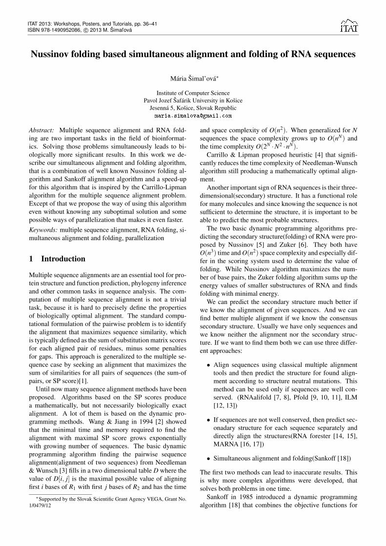
Nussinov folding based simultaneous alignment and folding of RNA sequences

Mária Šimal’ová∗

Institute of Computer SciencePavol Jozef Šafárik University in Košice

Jesenná 5, Košice, Slovak Republicmaria.simalova@gmail.com

Abstract: Multiple sequence alignment and RNA fold-ing are two important tasks in the field of bioinformat-ics. Solving those problems simultaneously leads to bi-ologically more significant results. In this work we de-scribe our simultaneous alignment and folding algorithm,that is a combination of well known Nussinov folding al-gorithm and Sankoff alignment algorithm and a speed-upfor this algorithm that is inspired by the Carrillo-Lipmanalgorithm for the multiple sequence alignment problem.Except of that we propose the way of using this algorithmeven without knowing any suboptimal solution and somepossible ways of parallelization that makes it even faster.Keywords: multiple sequence alignment, RNA folding, si-multaneous alignment and folding, parallelization

1 Introduction

Multiple sequence alignments are an essential tool for pro-tein structure and function prediction, phylogeny inferenceand other common tasks in sequence analysis. The com-putation of multiple sequence alignment is not a trivialtask, because it is hard to precisely define the propertiesof biologically optimal alignment. The standard compu-tational formulation of the pairwise problem is to identifythe alignment that maximizes sequence similarity, whichis typically defined as the sum of substitution matrix scoresfor each aligned pair of residues, minus some penaltiesfor gaps. This approach is generalized to the multiple se-quence case by seeking an alignment that maximizes thesum of similarities for all pairs of sequences (the sum-ofpairs, or SP score)[1].

Until now many sequence alignment methods have beenproposed. Algorithms based on the SP scores producea mathematically, but not necessarily biologically exactalignment. A lot of them is based on the dynamic pro-gramming methods. Wang & Jiang in 1994 [2] showedthat the minimal time and memory required to find thealignment with maximal SP score grows exponentiallywith growing number of sequences. The basic dynamicprogramming algorithm finding the pairwise sequencealignment(alignment of two sequences) from Needleman& Wunsch [3] fills in a two dimensional table D where thevalue of D[i, j] is the maximal possible value of aligningfirst i bases of R1 with first j bases of R2 and has the time

∗Supported by the Slovak Scientific Grant Agency VEGA, Grant No.1/0479/12

and space complexity of O(n2). When generalized for Nsequences the space complexity grows up to O(nN) andthe time complexity O(2N ·N2 ·nN).

Carrillo & Lipman proposed heuristic [4] that signifi-cantly reduces the time complexity of Needleman-Wunschalgorithm still producing a mathematically optimal align-ment.

Another important sign of RNA sequences is their three-dimensional(secondary) structure. It has a functional rolefor many molecules and since knowing the sequence is notsufficient to determine the structure, it is important to beable to predict the most probable structures.

The two basic dynamic programming algorithms pre-dicting the secondary structure(folding) of RNA were pro-posed by Nussinov [5] and Zuker [6]. They both haveO(n3) time and O(n2) space complexity and especially dif-fer in the scoring system used to determine the value offolding. While Nussinov algorithm maximizes the num-ber of base pairs, the Zuker folding algorithm sums up theenergy values of smaller substructures of RNA and findsfolding with minimal energy.

We can predict the secondary structure much better ifwe know the alignment of given sequences. And we canfind better multiple alignment if we know the consensussecondary structure. Usually we have only sequences andwe know neither the alignment nor the secondary struc-ture. If we want to find them both we can use three differ-ent approaches:

• Align sequences using classical multiple alignmenttools and then predict the structure for found align-ment according to structure neutral mutations. Thismethod can be used only if sequences are well con-served. (RNAalifold [7, 8], Pfold [9, 10, 11], ILM[12, 13])

• If sequences are not well conserved, then predict sec-onadary structure for each sequence separately anddirectly align the structures(RNA forester [14, 15],MARNA [16, 17])

• Simultaneous alignment and folding(Sankoff [18])

The first two methods can lead to inaccurate results. Thisis why more complex algorithms were developed, thatsolves both problems in one time.

Sankoff in 1985 introduced a dynamic programmingalgorithm [18] that combines the objective functions for

ITAT 2013: Workshops, Posters, and Tutorials, pp. 36–41ISBN 978-1490952086, c© 2013 M. Šimal’ová

alignment and minimal free energy folding to solve thealignment of finite sequences, their folding and the recon-struction of ancestral sequences on a phylogenetic tree.This algorithm is based on Sankoff alignment algorithm([19]), distance function for evaluating alignments by Sell-ers ([20, 21]) and on the Zuker and Sankoff paper [22],who synthesize and advance a series of improvements inalgorithmic efficiency including Nussinov algorithm andZuker algorithm.

Ziv-Ukelson et al. in [23] extended the approach from[24] for speeding up the classical Zuker’s folding algo-rithm to speed up the Sankoff’s algorithm for simultane-ous folding and alignment and get the time complexity ofO(n4 · ζ (n)) for two sequences, where ζ (n) goes to n forincreasing n.

There is also a few heuristic implementations of Sankoffalgorithm. One of them is Foldalign [25], which usesa combination of clustal [26] and consensus [27] heuris-tics to build multiple sequence alignment from pair-wisecomparison. Foldaling reduces the time complexity toO(n4 ·N)(N is the number of sequences, n is the length ofthe longest sequence) by restricting maximum motif sizeand forbidding multiloops. So it can be used only for shortsequences without multiloops.

Another heuristic implementation of Sankoff algorithmis Dynalign [28], which restricts the difference in indices iand j of aligned nucleotides to be less than M (i is a posi-tion in sequence S1 and j in sequence S j). It also limits thesize of internal loops to get the complexity of O(n3 ·M3).The disadvantage is that it is only restricted to pairwisesequence comparison.

There is more heuristic algorithms for simultaneousfolding and alignment from recent years, that reduceSankoff’s algorithm computational complexity. Theycan be found for example in Will et al.([29]), Kiryuet al.([30]) and Torarinsson([31]), all from 2007. Butalso Dowell, 2006([32]) and Holmes([33]), Uzilov etal.([34]), Havgaard et al.([35]) from 2005 and Hofackeret al.,2004([36]).

In the first part of this work, we describe two knownalgorithms. The Carrilo-Lipman multiple sequence align-ment algorithm and the Nussinov folding algorithm. Afterthis we describe our simultaneous alignment and foldingalgorithm based on the Nussinov folding scheme and ap-plication of Carrillo-Lipman heuristic to this algorithm. Inthe end we propose the way of using this algorithm withoutany previously known suboptimal alignment and a paral-lelization speed-up.

2 Carrillo-Lipman

The Carrillo & Lipman [4] algorithm for multiple se-quence alignment is dynamically filling in the matrix D us-ing equations from Needleman & Wunsch algorithm [3],but generalized for N sequences. The value of D[

−→i ] is

the maximal possible value of aligning first i1 bases ofR1 with first i2 bases of R2, ... and first iN bases of RN .

Let PermN0,1 be the set of all permutations of length Nfrom the set 0,1. The generalized equation is:

D[−→i ] = maxp∈PermN0,1

D[−−→i− p]+∑N

j=1 p j ∗ (N−∑Nj=1 p j)∗ y

+∑m,l∈1,...,N,pm=pl=1 C(Rm,im ,Rl,il )

(1)

The idea of Carrillo-Lipman heuristic is to cut off somecomputations, which we know will never lead to an opti-mal solution.

If we compute the value of optimal pairwise alignmentfor all pairs of sequences such that dm,l [im, il ] will be themaximal value for aligning subsequences Rm[im, ...,nm]and Rl [il , ...,nl ], then it is obvious that:

D[−→n ]−N

∑m=1

N

∑l=1

dm,l [im, il ]≤ D[−→i ] (2)

Suppose, we have some suboptimal multiple alignmentfound by any faster heuristic algorithm. Let U be the valueof this suboptimal alignment (U is less or equal to the op-timal alignment value). If the cell D[i1, i2, ..., iN ] will be apart of the optimal solution, then obviously:

D[−→i ]+

N

∑m=1

N

∑l=1

dm,l [im, il ]>=U (3)

So if the condition 3 is not satisfied, then the cellD[i1, i2, ..., iN ] is not a part of the optimal solution. Carrillo& Lipman compute the matrix values in the opposite di-rection. After improving cell D[i1, i2, ..., iN ], they improveall cells that can be affected by this change only if it sat-isfy the condition 3. That allows them to cut off a lot ofunnecessary computations.

3 Nussinov folding algorithm

The Nussinov algorithm predicts the secondary structureof RNA by maximizing of the number of base pairs, ac-cording to the assumption that the more base pairs containsthe sequence the more stable it is.

Let R be the input RNA sequence of length n. The al-gorithm fills in the matrix F of size n · n, where the valueof F [i, j] is the maximum number of possible base pairs insubsequence R[i... j]. The best structure for subsequenceR[i... j] is calculated from the previously calculated beststructures for smaller subsequences [37]. There are fourfollowing ways to fill in the value of F [i, j]:

• Add unpaired base i to the best secondary structurefor subsequence R[i+1, j](F [i, j] = F [i+1, j]).

• Add unpaired base j to the best secondary structurefor subsequence R[i, j−1](F [i, j] = F [i, j−1]).

• Add base pair (i, j) to the best secondary structure forsubsequence R[i+1, j−1](F [i, j] = F [i+ 1, j−1]+δ (i, j), where δ (i, j) is value of adding this kind ofpair).

Simultaneous Alignment and Folding of RNA Sequences 37

• Combination of the best secondary substructures forsubsequences R[i,k] and R[k+1, j] for some k ∈ i+1, ..., j−1. (F [i, j] = F [i,k]+F [k+1, j])

This leads to following equations, where 1 ≤ i ≤ n andi< j ≤ n :

F(i, j) = max

F [i+1, j]F [i, j−1]F [i+1, j−1]+δ (i, j)maxi<k< jF [i,k]+F [k+1, j]

(4)

F(i, i) = F(i, i+1) = 0 (5)

The matrix is filled, beginning with the initialization ac-cording to (5) and then computing the lower half fromsmaller to longer subsequences [37]. After filling the ma-trix the solution is recieved via backtracking beginningwith F [1,n] what is the maximum number of base pairsfor the whole sequence. The time complexity of Nussinovalgorithm is O(n3) because of filling in n2 cells by lookingat O(n) cells filled before. The space complexity is O(n2).

4 Simultaneous alignment and Nussinovfolding

Our objective is to explore, whether it is possible to applythe Carrillo-Lipman approach for multiple sequence align-ment to speed up simultaneous alignment and folding. Wedecided to try it at first with the Nussinov folding algo-rithm. The first step to this is to design an equation forsimultaneous alignment and Nussinov folding.

We combine the Sankoff alignment algorithm withNussinov folding algorithm like Sankoff[18] combined itwith Zuker folding algorithm. For two sequences we dis-tinguish five cases when filling in the value of F [i, j;k, l]:

• Add pairs of bases i, j and k, l, base i will be alignedto base k and base j will be aligned to base l. Thenthe value will be computed as sum of the valueF [i+ 1, j− 1;k+ 1, l− 1], the values of created basepairs δ (i, j)+ δ (k, l), and the value of aligned basesC(R1,i,R2,k)+C(R1, j,R2,l)

• Align unpaired nucleotides i and k to the best alignedstructures of sequences R1[i + 1, ..., j] and R2[k +1, ..., l].

• Align unpaired nucleotides j and l to the best alignedstructures of sequences R1[i, ..., j−1] and R2[k, ..., l−1].

• There are no base pairs in subsequences R1[i, ..., j]and R2[k, ..., l] so we have just to compute the valueof aligning those sequences.

• Combine two previously computed substructuresF [i,h;k, p] and F [h+1, j; p+1, l].

This four cases leads to the following equation:

F [i, j;k, l] = max

F [i+1, j−1;k+1, l−1]+δ (i, j)+δ (k, l)+C(R1,i,R2,k)+C(R1, j,R2,l)

F [i+1, j;k+1, l]+C(R1,i,R2,k)

F [i, j−1;k, l−1]+C(R1, j,R2,l)

D[i, j;k, l]maxi<h< j;k<p<lF [i,h;k, p]+F [h+1, j; p+1, l]

(6)

∀i, j : F [i, i−1; j, j−1] = 0 (7)

The space complexity here is O(n4) and the time com-plexity goes to O(n6) because of the fifth case.

We can also generalize it for N sequences (8). It needsO(n2·N) space and O(n3·N) time.

F [−→i, j] =max

F [−−−−−−→i+1, j−1]+∑N

k=1 δ (ik, jk)+∑N

m=1 ∑Nk=m+1 (C(Rm,im ,Rk,ik )+C(Rm, jm ,Rk, jk ))

F [−−−−→i+1, j]+∑N

m=1 ∑Nk=m+1 C(Rm,im ,Rk,ik )

F [−−−−→i, j−1]+∑N

m=1 ∑Nk=m+1 C(Rm, jm ,Rk, jk )

D[−→i, j]

maxim<hm< jm F [−→i,h]+F [

−−−−→h+1, j]

(8)

4.1 Applying Carrillo-Lipman approach tosimultaneous alignment and Nussinov folding

Suppose we have some suboptimal alignment and foldingof sequences R1,R2, ...,Rn with value U . We want to ap-ply the Carrillo-Lipman approach to our algorithm. At firstwe have to find the upper bound for the value of simulta-neous alignment and folding. The upper bound of align-ment value for subsequences R1[0, ..., i1], R2[0, ..., i2], ... ,RN [0, ..., iN ] is the sum of maximal pairwise alignmentsvalues for all pairs of sequences, same like in Carrillo-Lipman algorithm. The upper bound for simultaneous al-gorithm will be equal to sum of the upper bound for align-ment and the upper bound for secondary structures. Thevalue of secondary structure is added only in the first case.The value of every base pair in every sequence is added ex-actly once. Let fm(im, jm) be the value of best secondarystructure of subsequence Rm[0, ..., im − 1, jm + 1, ...,nm].So we can say, that:

F [−→0,n]−

N

∑m=1

fm(im, jm))−N

∑m=1

N

∑l=1

dm,l [im, il ]−N

∑m=1

N

∑l=1

d′m,l [ jm, jl ]≤F [−→i, j]

(9)

The cell F [−→i, j] can then be excluded from the compu-

tation if its value is so small that even if the alignmentand folding value of subsequences R1[0, ..., i1, j1, ...,n1],R2[0, ..., i2, j2, ...,n2], ... , RN [0, ..., iN , jN , ...,nN ] are maxi-mal:

N

∑m=1

N

∑l=m+1

dm,l [im, il ]+N

∑m=1

fm(im, jm)+N

∑m=1

N

∑l=m+1

d′m,l [ jm, jl ]

(10)

38 M. Šimal’ová

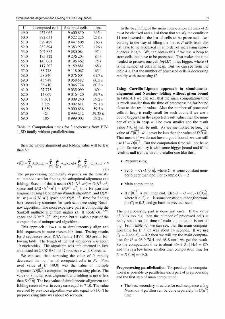
U # computed cells # skipped cells time49.0 457 062 9 600 830 335 s50.0 392 631 9 522 226 218 s51.0 329 429 9 447 505 163 s52.0 282 894 9 383 973 126 s53.0 207 882 9 280 084 97 s54.0 175 322 9 236 203 84 s55.0 143 061 9 196 462 75 s56.0 117 202 9 159 881 68 s57.0 88 778 9 118 067 65 s58.0 58 340 9 076 604 61.7 s59.0 45 948 9 058 582 60.5 s60.0 36 410 9 046 724 60.2 s61.0 27 773 9 035 099 60 s62.0 14 069 9 016 420 59.7 s63.0 9 301 9 009 240 59.2 s65.0 3 889 9 002 811 59.1 s66.0 1 859 9 000 656 59.3 s67.0 424 8 999 232 59.28 s69.0 185 8 999 003 59.2 s

Table 1: Computation times for 3 sequences from HIV-1_SD family without parallelization.

then the whole alignment and folding value will be lessthan U :

F [−→i, j]+

N

∑m=1

fm(im, jm)+N

∑m=1

N

∑l=m+1

dm,l [im, il ]+N

∑m=1

N

∑l=m+1

d′m,l [ jm, jl ]<U

(11)The preprocessing complexity depends on the heuristi-cal method used for finding the suboptimal alignment andfolding. Except of that it needs O(2 ·N2 ·n2) = O(N2 ·n2)space and O(2 · N2 · n2) = O(N2 · n2) time for pairwisealignment using Needleman-Wunsch algorithm, and O(N ·n2 · n2) = O(N · n4) space and O(N · n3) time for findingbest secondary structure for each sequence using Nussi-nov algorithm. The most expensive part is computing theSankoff multiple alignment matrix D. It needs O(n2·N)space and O(n2·N ·2N ·N2) time, but it is also a part of thecomputation of unimproved algorithm.

This approach allows us to simultaneously align andfold sequences in more reasonable time. Testing resultsfor 3 sequences from RNA family HIV-1_SD are in fol-lowing table. The length of the test sequences was about19 nucleotides. The algorithm was implemented in Javaand tested on 2.30GHz Intel i7 processor with 8 threads.

We can see, that increasing the value of U rapidlydecreased the number of computed cells in F . Firstused value of U (49.0) was the value of multiplealignment(D[

−→0,n]) computed in preprocessing phase. The

value of simultaneous alignment and folding is never lessthan D[

−→0,n]. The best value of simultaneous alignment and

folding received was in every case equal to 71.0. The valuereceived by previous algorithm was also equal to 71.0. Thepreprocessing time was about 45 seconds.

In the beginning of the main computation all cells of Dmust be checked and all of them that satisfy the condition11 are inserted to the list of cells to be processed. Ac-cording to the way of filling the matrix F cells from thislist have to be processed in an order of increasing subse-quences length. We can obtain this if we use a heap tostore cells that have to be processed. That makes the timeneeded to process one cell log(M) times bigger, where Mis the number of cells in heap. But we can see from thetable 4.1, that the number of processed cells is decreasingrapidly with increasing U .

Using Carrillo-Lipman approach to simultaneousalignment and Nussinov folding without given boundIn table 4.1 we can see, that the main computation timeis much smaller than the time of preprocessing for boundclose to the result value. Also the number of processedcells in heap is really small for such bound.If we use abound bigger than the expected result value, then the num-ber of cells in heap will be even smaller and the resultvalue F [

−→0,n] will be null. As we mentioned before, the

value of F [−→0,n] will never be less than the value of D[

−→0,n].

That means if we do not have a good bound, we can stilluse U = D[

−→0,n]. But the computation time will not be so

good. So we can try it with some bigger bound and if theresult is null try it with a bit smaller one like this:

• Preprocessing

• Set U =C1 ·D[−→0,n], where C1 is some constant num-

ber bigger than one. For example C1 = 2

• Main computation

• If F [−→0,n] is null, then end. Else U =U −C2 ·D[

−→0,n],

where 0<C2 < 1 is some constant number(for exam-ple C2 = 0.2) and go back to previous step.

The preprocessing part is done just once. If the valueof U is too big, then the number of processed cells isreally small, so the time of main computation is not sobig. From table 4.1 we can see, that the main computa-tion time for U ≥ 63 was about 14 seconds. If we useC1 = 2 and C2 = 0.2 then we will try the main computa-tion for U = 98.0,78.4 and 68.8 until we get the result.So the computation time is about 45s + 3 · (14s) = 87sand this is a few times smaller than computation time forU = D[

−→0,n] = 49.0.

Preprocessing parallelization To speed up the computa-tion it is possible to parallelize each part of preprocessingand the first step of main computation.

• The best secondary structure for each sequence usingNussinov algorithm can be done separately in O(n5)time.

Simultaneous Alignment and Folding of RNA Sequences 39

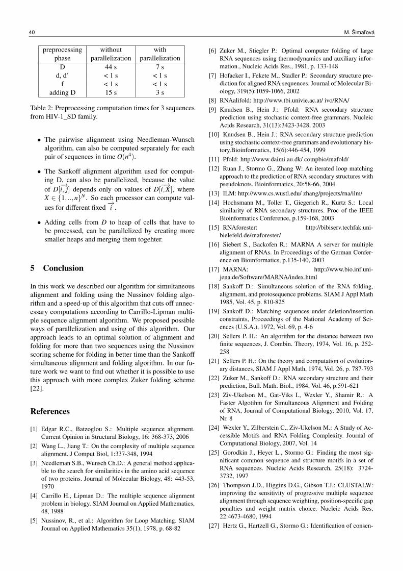
preprocessing without withphase parallelization parallelization

D 44 s 7 sd, d’ < 1 s < 1 s

f < 1 s < 1 sadding D 15 s 3 s

Table 2: Preprocessing computation times for 3 sequencesfrom HIV-1_SD family.

• The pairwise alignment using Needleman-Wunschalgorithm, can also be computed separately for eachpair of sequences in time O(n4).

• The Sankoff alignment algorithm used for comput-ing D, can also be parallelized, because the valueof D[

−→i, j] depends only on values of D[

−→i,X ], where

X ∈ 1, ..,nN . So each processor can compute val-ues for different fixed

−→i .

• Adding cells from D to heap of cells that have tobe processed, can be parallelized by creating moresmaller heaps and merging them togehter.

5 Conclusion

In this work we described our algorithm for simultaneousalignment and folding using the Nussinov folding algo-rithm and a speed-up of this algorithm that cuts off unnec-essary computations according to Carrillo-Lipman multi-ple sequence alignment algorithm. We proposed possibleways of parallelization and using of this algorithm. Ourapproach leads to an optimal solution of alignment andfolding for more than two sequences using the Nussinovscoring scheme for folding in better time than the Sankoffsimultaneous alignment and folding algorithm. In our fu-ture work we want to find out whether it is possible to usethis approach with more complex Zuker folding scheme[22].

References

[1] Edgar R.C., Batzoglou S.: Multiple sequence alignment.Current Opinion in Structural Biology, 16: 368-373, 2006

[2] Wang L., Jiang T.: On the complexity of multiple sequencealignment. J Comput Biol, 1:337-348, 1994

[3] Needleman S.B., Wunsch Ch.D.: A general method applica-ble to the search for similarities in the amino acid sequenceof two proteins. Journal of Molecular Biology, 48: 443-53,1970

[4] Carrillo H., Lipman D.: The multiple sequence alignmentproblem in biology. SIAM Journal on Applied Mathematics,48, 1988

[5] Nussinov, R., et al.: Algorithm for Loop Matching. SIAMJournal on Applied Mathematics 35(1), 1978, p. 68-82

[6] Zuker M., Stiegler P.: Optimal computer folding of largeRNA sequences using thermodynamics and auxiliary infor-mation., Nucleic Acids Res., 1981, p. 133-148

[7] Hofacker I., Fekete M., Stadler P.: Secondary structure pre-diction for aligned RNA sequences. Journal of Molecular Bi-ology, 319(5):1059-1066, 2002

[8] RNAalifold: http://www.tbi.univie.ac.at/ ivo/RNA/[9] Knudsen B., Hein J.: Pfold: RNA secondary structure

prediction using stochastic context-free grammars. NucleicAcids Research, 31(13):3423-3428, 2003

[10] Knudsen B., Hein J.: RNA secondary structure predictionusing stochastic context-free grammars and evolutionary his-tory.Bioinformatics, 15(6):446-454, 1999

[11] Pfold: http://www.daimi.au.dk/ compbio/rnafold/[12] Ruan J., Stormo G., Zhang W: An iterated loop matching

approach to the prediction of RNA secondary structures withpseudoknots. Bioinformatics, 20:58-66, 2004

[13] ILM: http://www.cs.wustl.edu/ zhang/projects/rna/ilm/[14] Hochsmann M., Toller T., Giegerich R., Kurtz S.: Local

similarity of RNA secondary structures. Proc of the IEEEBioinformatics Conference, p.159-168, 2003

[15] RNAforester: http://bibiserv.techfak.uni-bielefeld.de/rnaforester/

[16] Siebert S., Backofen R.: MARNA A server for multiplealignment of RNAs. In Proceedings of the German Confer-ence on Bioinformatics, p.135-140, 2003

[17] MARNA: http://www.bio.inf.uni-jena.de/Software/MARNA/index.html

[18] Sankoff D.: Simultaneous solution of the RNA folding,alignment, and protosequence problems. SIAM J Appl Math1985, Vol. 45, p. 810-825

[19] Sankoff D.: Matching sequences under deletion/insertionconstraints, Proceedings of the National Academy of Sci-ences (U.S.A.), 1972, Vol. 69, p. 4-6

[20] Sellers P. H.: An algorithm for the distance between twofinite sequences, J. Combin. Theory, 1974, Vol. 16, p. 252-258

[21] Sellers P. H.: On the theory and computation of evolution-ary distances, SIAM J Appl Math, 1974, Vol. 26, p. 787-793

[22] Zuker M., Sankoff D.: RNA secondary structure and theirprediction, Bull. Math. Biol., 1984, Vol. 46, p.591-621

[23] Ziv-Ukelson M., Gat-Viks I., Wexler Y., Shamir R.: AFaster Algotihm for Simultaneous Alignment and Foldingof RNA, Journal of Computational Biology, 2010, Vol. 17,Nr. 8

[24] Wexler Y., Zilberstein C., Ziv-Ukelson M.: A Study of Ac-cessible Motifs and RNA Folding Complexity. Journal ofComputational Biology, 2007, Vol. 14

[25] Gorodkin J., Heyer L., Stormo G.: Finding the most sig-nificant common sequence and structure motifs in a set ofRNA sequences. Nucleic Acids Research, 25(18): 3724-3732, 1997

[26] Thompson J.D., Higgins D.G., Gibson T.J.: CLUSTALW:improving the sensitivity of progressive multiple sequencealignment through sequence weighting, position-specific gappenalties and weight matrix choice. Nucleic Acids Res,22:4673-4680, 1994

[27] Hertz G., Hartzell G., Stormo G.: Identification of consen-

40 M. Šimal’ová

sus patterns in unaligned DNA sequences known to be func-tionally related. Comput Appl Biosci, 6: 81-92, 1990

[28] Mathews D., Turner D.: Dynalign: An algorithm for find-ing the secondary structure common to two RNA sequences.Journal of Molecular Biology, 317(2):191-203, 2002

[29] Will S., Reiche K., Hofacker I.L., et al.: Inferring non-coding RNA families and classes by means of genome-scalestructure-based clustering. PLOS Comput. Biol, Vol. 3, 2007

[30] Kiryu H., Tabei Y., Kin T., et al.: MURLET: a practicalmultiple alignmetn tool for structural alignment sequences.Bioinformatics, 23: 1588-1598, 2007

[31] Torarinsson E., Havgaard J.H., Gorodkin J.: Multiple struc-tural alignment and clustering of RNA sequences. Bioinfor-matics 23:926-932,2007

[32] Dowel R.D., Eddy S.: Efficient pairwise RNA structureprediction and alignment using sequence alignment con-straints. BMC Bioinform. 7: 400, 2006

[33] Holmes I.: Accelerated probabilistic inference of RNAstructure evolution. BMC Biooinform. 6:73, 2005

[34] Uzilov A.V., Keegan J.M., Mathews D.H.: Detection ofnon-coding RNAs on the basis predicted secondary structureformation free energy change. BMC Bioinform. 7:173, 2005

[35] Havgaard J.H., Lyngso R.B., Stormo G.D., et al.: Pair-wise local structural alignment of RNA sequences with se-quence similarity less than 40%. Bioinformatics 21: 1815-1824, 2005

[36] Hofacker I.L., Bernhart S., Stadler P.: Alignment of RNAbase pairing probability matrices. Bioinformatics 20: 2222-2227, 2004

[37] Sperschneider V., Sperschneider J., Scheubert L.: Bioinfor-matics: problem solving paradigms. Springer, 2008

Simultaneous Alignment and Folding of RNA Sequences 41

In silico search for secondary structures in p53 target genes usingR/Bioconductor

Marie Brázdová1, Tomáš Martínek2, and Matej Lexa3

1 Biophysical Institute of the Czech Academy of Sciences, Královopolská 135, 61265 Brno, Czech Republicmaruska@ibp.cz

2 Faculty of Informatics, Masaryk University, Botanická 68a, 60200 Brno, Czech Republic, lexa@fi.muni.cz3 Faculty of Information Technology, Brno Technical University, Božetechova 1/2, 61266 Brno, Czech Republic,

martinto@fit.vutbr.cz

Abstract: p53 is a well-known transcription factor andtumor suppressor, regulating among other processes, thecommitment of cells to apoptosis and DNA repair. p53mutants are often found in cancers of different kinds, ei-ther as mutant or misregulated p53. p53 is involved inmany other processes and we currently do not understandthe full range of its functions. It is known to recognizethe p53con sequence by its specific DNA-binding domain(DBD). It is also known to bind DNA non-specifically.This binding has been shown to involve superhelical DNA,more specifically, cruciform, triplex and quadruplex struc-tures. In our laboratories we were intrigued by the possi-ble interplay between non-canonical DNA structure bind-ing and regular p53con binding. In an attempt to clarifythis interplay and discover suitable candidate genes for fur-ther study, we carried out an in silico study on the humangenome. We identified all the occurences of potential cru-ciform DNA, triplex DNA, quadruplex DNA and p53conrecognition sequences in +/-40000 bp regions of knowngenes. We analyzed this data for statistically significantpatterns and combinations of patterns using a small set ofavailable R/Bioconductor packages. This paper describesthe computational pipeline designed for this type of stud-ies. We also show preliminary results for selected humansequences.

1 Introduction

The existence of non-canonical DNA (also non-B DNA)with secondary structure different from the B-DNA formdescribed by Crick and Watson [1] has been known forsom time now. Cruciform, slipped, triplex or quadru-plex DNA has been recognized as a factor in several im-portant biological processes or functions. The structureshave the ability to modulate replication [2], transcription[3] or translation [4] of DNA/RNA by mechanisms thatmay have their origins in times when nucleic acids domi-nated all life processes [5]. Their possible functions maybe globally regulated by the overall topology of DNA incells, since their existence is thermodynamically possibleonly above/below certain superhelicity thresholds.

p53 belongs to a small group of proteins capable ofnon-specifically binding non-B DNA, such as cruciformor quadruplex DNA [6]. Because of its importance as a tu-

mor supressor (in its wt-p53 form) or tumor activator (mut-p53), we would like to better understand the relationshipbetween human p53 function and non-B DNA structurespresent in the human genome. While many experimentshave previously addressed this issue [6][7], we still do notproperly understand the interplay between DNA topologi-cal status, gene regulation, cell fate and p53.

In this paper, we describe the possibilities for in silicostudies of possible relationships by analyzing the humangenome sequence or sequences of selected genes and theirimmediate surroundings. To carry out such study, we takeadvantage of our own software for detecting potential in-tramolecular triplexes (H-DNA) and the existing R/Bio-conductor framework, to efficiently locate and evaluate allsequences capable of forming non-B DNA or attractingp53 in a more sequence-specific manner.

Using this approach we were able to find over- or under-representation of sequence patterns in the vicinity of genetranscription start sites (TSS) and p53con sequences.

2 Software

2.1 R/Bioconductor

To analyze the human genome, or other sequence set, weemploy the R/Bioconductor framework, which has nowmatured to the point, where we can use R to represent bi-ological sequences, search these sequences, represent thesearch results, analyze them statistically and visualize theresults of the searchs and the statistical analysis. All thiscan be done with relatively straightforward scripts, using ahandful of well integrated R/Bioconductor software pack-ages.

Packages used in this study include:

Biostrings String objects representing biological se-quences, and matching algorithms[8]

BSgenome Infrastructure for Biostrings-based genomedata packages[9]

BSgenome.Hsapiens.UCSC.hg19 Homo sapiens (Hu-man) full genome (UCSC version hg19)

biomaRt Interface to BioMart databases (e.g. Ensembl,COSMIC ,Wormbase and Gramene)[10]

ITAT 2013: Workshops, Posters, and Tutorials, pp. 42–46ISBN 978-1490952086, c© 2013 M. Brázdová, T. Martínek, M. Lexa

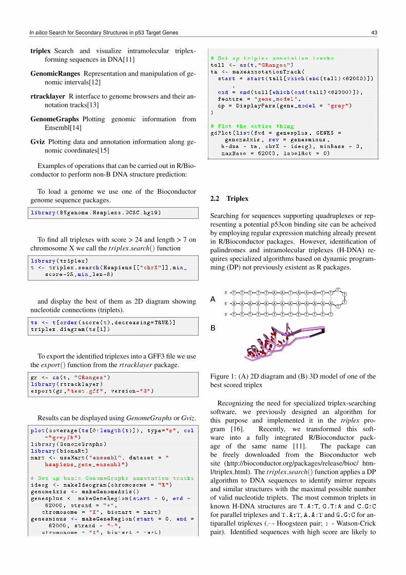
triplex Search and visualize intramolecular triplex-forming sequences in DNA[11]

GenomicRanges Representation and manipulation of ge-nomic intervals[12]

rtracklayer R interface to genome browsers and their an-notation tracks[13]

GenomeGraphs Plotting genomic information fromEnsembl[14]

Gviz Plotting data and annotation information along ge-nomic coordinates[15]

Examples of operations that can be carried out in R/Bio-conductor to perform non-B DNA structure prediction:

To load a genome we use one of the Bioconductorgenome sequence packages.

1 library(BSgenome.Hsapiens.UCSC.hg19)

To find all triplexes with score > 24 and length > 7 onchromosome X we call the triplex.search() function

1 library(triplex)

2 t <- triplex.search(Hsapiens [["chrX"]],min_

score=25,min_len=8)

and display the best of them as 2D diagram showingnucleotide connections (triplets).

1 ts <- t[order(score(t),decreasing=TRUE)]

2 triplex.diagram(ts[1])

To export the identified triplexes into a GFF3 file we usethe export() function from the rtracklayer package.

1 gr <- as(t, "GRanges")

2 library(rtracklayer)

3 export(gr ,"test.gff", version="3")

Results can be displayed using GenomeGraphs or Gviz.

1 plot(coverage(ts[0: length(t)]), type="s", col

="grey75")

2 library(GenomeGraphs)

3 library(biomaRt)

4 mart <- useMart("ensembl", dataset = "

hsapiens_gene_ensembl")

5

6 # Set up basic GenomeGraphs annotation tracks

7 ideog <- makeIdeogram(chromosome = "X")

8 genomeAxis <- makeGenomeAxis ()

9 genesplus <- makeGeneRegion(start = 0, end =

62000, strand = "+",

10 chromosome = "X", biomart = mart)

11 genesminus <- makeGeneRegion(start = 0, end =

62000, strand = "-",

12 chromosome = "X", biomart = mart)

13

14 # Set up triplex annotation tracks

15 tall <- as(t,"GRanges")

16 ta <- makeAnnotationTrack(

17 start = start(tall[which(end(tall) <62000)])

,

18 end = end(tall[which(end(tall) <62000)]),

19 feature = "gene_model",

20 dp = DisplayPars(gene_model = "grey")

21 )

22

23 # Plot the entire thing

24 gdPlot(list(fwd = genesplus , GENES =

genomeAxis , rev = genesminus ,

25 h-dna = ta, chrX = ideog), minBase = 0,

26 maxBase = 62000 , labelRot = 0)

2.2 Triplex

Searching for sequences supporting quadruplexes or rep-resenting a potential p53con binding site can be acheivedby employing regular expression matching already presentin R/Bioconductor packages. However, identification ofpalindromes and intramolecular triplexes (H-DNA) re-quires specialized algorithms based on dynamic program-ming (DP) not previously existent as R packages.

Figure 1: (A) 2D diagram and (B) 3D model of one of thebest scored triplex

Recognizing the need for specialized triplex-searchingsoftware, we previously designed an algorithm forthis purpose and implemented it in the triplex pro-gram [16]. Recently, we transformed this soft-ware into a fully integrated R/Bioconductor pack-age of the same name [11]. The package canbe freely downloaded from the Bioconductor website (http://bioconductor.org/packages/release/bioc/ htm-l/triplex.html). The triplex.search() function applies a DPalgorithm to DNA sequences to identify mirror repeatsand similar structures with the maximal possible numberof valid nucleotide triplets. The most common triplets inknown H-DNA structures are T.A:T, G.T:A and C.G:C

for parallel triplexes and T.A:T, A.A:T and G.G:C for an-tiparallel triplexes (. - Hoogsteen pair; : - Watson-Crickpair). Identified sequences with high score are likely to

In silico Search for Secondary Structures in p53 Target Genes 43

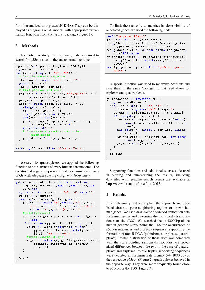
form intramolecular triplexes (H-DNA). They can be dis-played as diagrams or 3D models with appropriate visual-ization functions from the triplex package (Figure 1).

3 Methods

In this particular study, the following code was used tosearch for p53con sites in the entire human genome

1 hgenome <- BSgenome.Hsapiens.UCSC.hg19

2 gr_p53cons <- GRanges ()

3 for (i in c(seq (22), "Y", "X"))

4 # Get chromosome sequence

5 chr_name <- paste("chr",i,sep="")

6 print(chr_name)

7 chr <- hgenome [[chr_name]]

8 # Find p53cons and sort

9 p53_half <- matchPattern("RRRCWWGYYY", chr ,

max.mismatch=1, fixed=FALSE)

10 p53_gaps <- gaps(p53_half)

11 hits <- which(width(p53_gaps) <= 18)

12 if(length(hits) > 0)

13 p53 <- p53_gaps[hits]

14 start(p53) <- start(p53) -10

15 end(p53) <- end(p53)+10

16 gr <- GRanges(seqnames=chr_name , ranges=

ranges(p53), strand="*")

17 print(length(gr))

18 # Concatenate results with other

chromosomes

19 gr_p53cons <- c(gr_p53cons , gr)

20

21

22 save(gr_p53cons , file="p53cons.RData")

To search for quadruplexes, we applied the followingfunction to both strands of every human chromosome. Theconstructed regular expression matches consecutive runsof Gs with adequate spacing (loop_min, loop_max).

1 get_strand_quadruplexes <- function(seq ,

seqname , strand , g_min , g_max , loop_min ,

loop_max)

2 symbol <- if (strand == "+") "G" else "C"

3 gr_gg <- GRanges ()

4 for (g_len in seq(g_min , g_max))

5 pattern <- paste("(",symbol ,"",g_len ,"

.",loop_min ,",",loop_max ,")3,",

symbol ,"",g_len ,"",sep="")

6 #print(pattern)

7 ggroups <- gregexpr(pattern , seq , ignore.

case=T)

8 if(as.vector(ggroups [[1]]) [1] != -1)

9 ir_gg <- IRanges(start=as.vector(

ggroups [[1]]) , width=attr(ggroups

[[1]] , "match.length"))

10 #print(length(ir_gg))

11 gr_gg <- union(gr_gg, GRanges(seqnames=

seqname , ranges=ir_gg , strand=

strand))

12

13

14 gr_gg

15

To limit the sets only to matches in close vicinity ofannotated genes, we used the following code.

1 load("bm_genes.RData")

2 gr_tss <- get_tss_gr(bm_genes)

3 tss_p53con_hits <- distanceToNearest(gr_tss ,

gr_p53cons , ignore.strand=TRUE)

4 tss_p53con_dist <- as.data.frame(tss_p53con_

hits)$distance

5 gr_p53cons_genes <- gr_p53cons[subjectHits(

tss_p53con_hits)[which(tss_p53con_dist <

40000) ]]

6 save(gr_p53cons_genes , file="p53cons_genes.

RData")

A special function was used to ranomize positions andsave them in the same GRanges format used above fortriplexes and quadruplexes.

1 gr_randomize <- function(gr)

2 gr_rand <- GRanges ()

3 for(i in c(seq (22), "X", "Y"))

4 chr_name <- paste("chr",i,sep="")

5 gr_chr <- gr[seqnames(gr) == chr_name]

6 if (length(gr_chr) > 0)

7 chr_len <- seqlengths(hgenome)[which(

names(seqlengths(hgenome)) == chr_

name)]

8 new_start <- sample (1:chr_len , length(

gr_chr))

9 gr_chr_rand <- shift(gr_chr , new_start -

start(ranges(gr_chr)))

10 gr_rand <- c(gr_rand , gr_chr_rand)

11

12

13 gr_rand

14

Supporting functions and additional source code usedin plotting and summarizing the results, includingdata files with genome search results are available athttp://www.fi.muni.cz/ lexa/itat_2013.

4 Results

In a preliminary test we applied the approach and codelisted above to gene-neighboring regions of known hu-man genes. We used biomaRt to download annotation datafor human genes and determine the most likely transcrip-tion start site (TSS). We searched the +/-40000bp of thehuman genome surrounding the TSS for occurrences ofp53con sequences and close-by sequences supporting theformation of non-B DNA (palindromes, triplexes, quadru-plexes). When distribution of these sites was comparedwith the corresponding random distributions, we recog-nized differences between the two in the case of quadru-plexes and triplexes. While triplex-supporting sequenceswere depleted in the immediate vicinity (+/- 1000 bp) ofthe respective p53con (Figure 2), quadruplexes behaved inthe opposite way. They were more frequently found closeto p53con or the TSS (Figure 3).

44 M. Brázdová, T. Martínek, M. Lexa

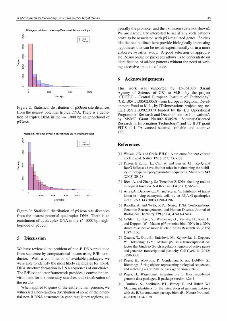
Figure 2: Statistical distribution of p53con site distancesfrom the nearest potential triplex DNA. There is a deple-tion of triplex DNA in the +/- 1000 bp neighborhood ofp53con.

Figure 3: Statistical distribution of p53con site distancesfrom the nearest potential quadruplex DNA. There is anenrichment of quadruplex DNA in the +/- 1000 bp neigh-borhood of p53con.

5 Discussion

We have reviewed the problem of non-B DNA predictionfrom sequence by computational means using R/Biocon-ductor. With a combination of available packages, wewere able to identify the most likely candidates for non-BDNA structure formation in DNA sequences of our choice.The R/Bioconductor framework provides a convenient en-vironment for the necessary searches and visualization ofthe results.

When applied to genes of the entire human genome, wewitnessed a non-random distribution of some of the poten-tial non-B DNA structures in gene regulatory regions, es-

pecially the promoter and the 1st intron (data not shown).We are particularly interested to see if any such patternsprove to be associated with p53-regulated genes. Studieslike the one outlined here provide biologically interestinghypotheses that can be tested experimentally or in a moreelaborate in silico study. A good selection of appropri-ate R/Bioconductor packages allows us to concentrate onidentification of ad-hoc patterns without the need of writ-ing excessive amounts of code.

6 Acknowledgements

This work was supported by 13-36108S (GrantAgency of Science of CR) to M.B., by the project“CEITEC - Central European Institute of Technology”(CZ.1.05/1.1.00/02.0068) from European Regional Devel-opment Fund to M.L., by IT4Innovations project, reg. no.CZ.1.05/1.1.00/02.0070 funded by the EU OperationalProgramme ’Research and Development for Innovations’,by MSMT Grant No.0021630528 ”Security-OrientedResearch in Information Technology” and by BUT grantFIT-S-11-1 ”Advanced secured, reliable and adaptiveIT”.

References

[1] Watson, J.D. and Crick, F.H.C.: A structure for deoxyribosenucleic acid. Nature 171 (1953) 737-738

[2] Dixon, B.P., Lu, L., Chu, A. and Bissler, J.J.: RecQ andRecG helicases have distinct roles in maintaining the stabil-ity of polypurine.polypyrimidine sequences. Mutat Res 643(2008) 20–28

[3] Rich, A. and Zhang, S.: Timeline: Z-DNA: the long road tobiological function. Nat Rev Genet 4 (2003) 566-72.

[4] Arora,A., Dutkiewicz, M. and Scaria, V.: Inhibition of trans-lation in living eukaryotic cells by an RNA G-quadruplexmotif. RNA 14 (2008) 1290–1296

[5] Bacolla, A. and Wells, R.D.: Non-B DNA Conformations,Genomic Rearrangements, and Human Disease. Journal ofBiological Chemistry 279 (2004) 47411-47414.

[6] Göhler, T., Jäger, S., Warnecke, G., Yasuda, H., Kim, E.and Deppert, W.: Mutant p53 proteins bind DNA in a DNAstructure-selective mode Nucleic Acids Research 33 (2005)1087-1100.

[7] Quante, T., Otto, B., Brázdová, M., Kejnovská, I., Deppert,W., Tolstonog, G.V.: Mutant p53 is a transcriptional co-factor that binds to G-rich regulatory regions of active genesand generates transcriptional plasticity. Cell Cycle 11 (2012)3290-3303.

[8] Pages, H., Aboyoun, P., Gentleman, R. and DebRoy, S.:Biostrings: String objects representing biological sequences,and matching algorithms. R package version 2.26.3.

[9] Pages, H.: BSgenome: Infrastructure for Biostrings-basedgenome data packages. R package version 1.26.1

[10] Durinck, S., Spellman, P.T., Birney, E. and Huber, W.:Mapping identifiers for the integration of genomic datasetswith the R/Bioconductor package biomaRt. Nature Protocols4 (2009) 1184-1191.

In silico Search for Secondary Structures in p53 Target Genes 45

[11] Hon, J., Martinek, T., Rajdl, K. and Lexa, M.: Triplex:an R/Bioconductor package for identification and visualiza-tion of potential intramolecular triplex patterns in DNA se-quences. Bioinformatics (in press).

[12] Aboyoun, P., Pages, H. and Lawrence, M.: Genomi-cRanges: Representation and manipulation of genomic in-tervals. R package version 1.10.7.

[13] Lawrence, M., Gentleman, R. and Carey, V.: rtracklayer:an R package for interfacing with genome browsers. Bioin-formatics 25 (2009) 1841-1842.

[14] Durinck, S. and Bullard, J.: GenomeGraphs: Plotting ge-nomic information from Ensembl. R package version 1.18.0.

[15] Hahne, F., Durinck, S., Ivanek, R., Mueller, A. andLianoglou, S.: Gviz: Plotting data and annotation informa-tion along genomic coordinates. R package version 1.2.1.

[16] Lexa, M., Martinek, T., Burgetova, I., Kopecek, D. andBrazdova, M.: A dynamic programming algorithm for iden-tification of triplex-forming sequences. Bioinformatics 27(2011) 2010-2017.

46 M. Brázdová, T. Martínek, M. Lexa

RNArobo: Fast RNA Motif Search(Abstract)

Ladislav Rampášek1,3, Andrej Lupták2, Tomáš Vinar3, and Brona Brejová3

1 Department of Computer Science, University of Toronto, Toronto, ON M5R 3G4 Canada2 Department of Pharmaceutical Sciences, Chemistry and Molecular Biology, University of California, Irvine,

2141 Natural Sciences 2, Irvine, CA 926973 Faculty of Mathematics, Physics, and Informatics, Comenius University, Mlynská Dolina, 842 48 Bratislava, Slovakia

RNA sequences are generally more conserved in theirstructure than in sequence. Thus to find RNAs related toa known example, we look for sequences capable of as-suming appropriate secondary structure. We investigatethe problem of RNA motif search based on user-defineddescriptors. RNA motif descriptors specify restrictionson base-pairing structure of the target RNA, as well assequence constraints characterizing conserved functionalsites. As opposed to popular fully-automated systemsbased on probabilistic models, this approach allows experthuman users to handcraft motif descriptors and highlightthe most important features of the target RNAs, thus bettertargeting a particular biological phenomenon.

The problem of descriptor-based RNA-motif search isNP-hard [1]. Nevertheless, effective search methods havebeen developed using either backtracking (e.g., RNAMot[2]), non-deterministic finite-state automata with noderewriting (e.g. RNAbob [3]), or dynamic programming forstructures without pseudoknots (e.g. Locomotif [4]). Mostof the other tools are based on one of these ideas, differ-ing in descriptor capabilities and post-processing options;extensive review can be found in [5].

Our new tool, RNArobo, builds on the descriptor for-mat of RNAbob and employs the backtracking algorithmof RNAMot. We improve these tools in two ways. First,we extend the RNAbob descriptor format to allow inser-tions, which is very useful for RNA structures that toleratebulges in their helices. Our main contribution, however,is a technique for improving the running time of the back-tracking algorithm.

The performance of backtracking depends greatly onordering of elements in the search. Each RNA structuredescriptor consists of several structural elements. In ouralgorithm, individual elements are aligned to the DNA se-quence by dynamic programming, with backtracking guid-ing the search for successive elements to appropriate loca-tions with respect to the already matched elements.

Ideally, the first elements will have few matches, fil-tering out most of the sequence from further processing.Such filtering is a common theme in many text searchmethods, such as the popular sequence similarity searchtool BLAST [6]. Different element orderings in the back-tracking search result in significant differences in runningtime. Finding the best ordering is an interesting and non-trivial problem, due to complex dependencies between lo-

cations of individual element. We approach this as anon-line problem, using the observed performance of thesearch so far to adjust ordering on-the-fly.

Using several realistic motif descriptors on the wholehuman genome, we demonstrate that for complex de-scriptors our strategy leads to a significant reduction inrunning time compared to existing tools RNAbob 2.2(1999) [3] and RNAmotif 3.0.7 (2010) [7]. Our softwaretool RNArobo is available at http://compbio.fmph.

uniba.sk/rnarobo

Acknowledgments. This research was supported by VEGAgrant 1/1085/12.

References

[1] L. Rampášek. RNA structural motif search is NP-complete. In Proceedings of the Student Science Con-ference 2011, Faculty of Mathematics, Physics and In-formatics, Comenius University in Bratislava, pages 341–348, 2011. http://compbio.fmph.uniba.sk/svk2011/svk2011-zbornik.pdf.

[2] D. Gautheret, F. Major, and R. Cedergren. Pattern search-ing/alignment with RNA primary and secondary structures:an effective descriptor for tRNA. Comput Appl Biosci,6(4):325–31, 1990.

[3] S.R. Eddy. RNABob: a program to search for RNA sec-ondary structure motifs in sequence databases. unpublished,1996.

[4] J. Reeder, J. Reeder, and R. Giegerich. Locomotif: fromgraphical motif description to RNA motif search. Bioinfor-matics, 23(13):i392–i400, 2007.

[5] A. D. George and S. A. Tenenbaum. Informatic resourcesfor identifying and annotating structural RNA motifs. MolBiotechnol, 41(2):180–93, 2009.

[6] S. F. Altschul, W. Gish, W. Miller, E. W. Myers, and D. J.Lipman. Basic local alignment search tool. Journal ofMolecular Biology, 215(3):403–410, 1990.

[7] T. J. Macke, D. J. Ecker, R. R. Gutell, D. Gautheret, D. A.Case, and R. Sampath. RNAMotif, an RNA secondarystructure definition and search algorithm. Nucl. Acids Res.,29(22):4724–4735, 2001.

ITAT 2013: Workshops, Posters, and Tutorials, p. 47ISBN 978-1490952086, c© 2013 L. Rampášek, A. Lupták, T. Vinar, B. Brejová

Integrating mRNA and miRNA expression with interaction knowledge todifferentiate myelodysplastic syndrome

Michael Andel1, Jirí Kléma1, and Zdenek Krejcík2

1 Department of Computer Science and Engineering, Prague, Czech Republic,andelmi2,klema@fel.cvut.cz,

2 Institute of Hematology and Blood Transfusion, Prague, Czech Republic,zdenek.krejcik@uhkt.cz

Abstract: Onset and progression of a genetically condi-tioned disease depend not only on genes themselves, butmainly on their expression during transcriptional and pro-teosynthetic process. Monitoring gene expression merelyat its transcription level often proves insufficient for an au-tomated disease understanding and prediction. An integra-tion of diverse high-throughput measurements and priorknowledge is needed to capture gene expression in a holis-tic way. In this paper, we apply a recent matrix factor-ization integration method to build a plausible and com-prehensive predictive model of an outcome or progressof myelodysplastic syndrome, a blood production diseaseoften progressing to leukemia. We propose an efficientlearning methodology that enables to maximize predic-tive performance and keep the main assets of the orig-inal method. The resulting model shows a comparablepredictive accuracy with a straightforward data integra-tion method while being more understandable and com-pact. The identified gene expression regulatory units withthe best predictive performance will be subject of furtherbiological analysis.

1 Introduction

A lot of severe diseases are genetically conditioned. Theoutcome or progress of such a disease depends not onlyon the patient’s genome, but also on the manifestationof certain genes. The overall gene activity during thetranscriptional-translational process is calledgene expres-sion (GE). It is the process through which genes synthe-size their products and afflict the phenotype. It is possibleto sense the activity of a gene as the measured amountof gene transcripts during its expression process. Currenttechnological progress enables to measure the activity ofthousands of genes simultaneously in one tissue sample.One may so feel being capable of predicting the diseaseoutcome, progress or related issues based on acquiredgeneexpression data[7]. In other words, to build a molecularclassifier with particular genes as features, gene expressionlevels as feature values and phenotype as target variable.

Nevertheless, recent studies suggest that such a molec-ular classifier based solely on GE data is often not suffi-ciently accurate nor understandable [5]. The lack of ac-curacy can be caused by technical difficulties such as thenoise in data as well as immense number of features. Too

many features may lead to overfitting, not to mention thefeatures are often redundant, irrelevant or highly depen-dent. As a reaction to this observation, the prevailing trendin GE data classification is focused on considering entiresets of genes rather than particular genes as the features[1, 8, 11, 15]. The gene sets are related to known or yetunknown biological processes as gene transcription regu-lation or metabolic pathways. Current effort is to refor-mulate GE features to gene sets and build models uponwhole biological processes. Resulting models should bemore precise, robust and, of course, biologically meaning-ful and more understandable for the experts.

But still, the results of set-level models may turn outdisappointing. Gene expression is a complex process withmultiple phases and components, which makes measure-ment of gene activity non-trivial. The acquired data areoften confusing in their nature and difficult to interpret andapply. Current molecular biology addresses this difficultythrough monitoring the activity of gene expression withinmultiple components at more stages of the process. Themultilevel measurement of GE results in potentially moreinformative, but much larger data. Therefore another chal-lenge for data analysis raises. A meaningful and compre-hensive integration of multiple measurements or multipledata sources is desirable.

In this work we propose a robust classification frame-work for knowledge-based integration of molecular ex-pression data. Currently, our quantitative measurementscover two fundamental transcript types: messenger RNA(mRNA) and microRNA (miRNA), both the crucial com-ponents of the overall gene expression process. mRNAserves as a carrier of genetic information from DNA toproteins. miRNA is a small non-coding molecule actingin transcriptional and post-transcriptional regulation,oftenhastening mRNA degradation and inhibiting translation ofa complementary mRNA into protein. Our challenge isto integrate the measurements of these different types ofribonucleic acids in a biologically meaningful way withgreat regard to the predictive accuracy of resulting mod-els. The integration is driven by the existing knowledgeon miRNA targets and gene-gene interactions. The ulti-mate goal is a valid and robust decision support tool forimmediate use in clinical or experimental practice.

The framework is tested on a particular domain ofmyelodysplastic syndrome(MDS) [23]. The data were

ITAT 2013: Workshops, Posters, and Tutorials, pp. 48–55ISBN 978-1490952086, c© 2013 M. Andel, J. Kléma, Z. Krejcík

provided by the Institute of Hematology and Blood Trans-fusion in Prague. MDS obstructs blood stem cells in bonemarrow from maturation, resulting in shortage of healthyblood cells. Consequent symptoms are anemia, increasedsusceptibility to bleeding and infection. What is more,great deal of MDS patients progress to treatment resis-tant acute myeloid leukaemia. Although many patients areasymptotic, the leukaemia may come out, though. An-other issue, reflected in the data is thechromosome 5qdeletion syndrome(del(5q)). del(5q) has similar symp-toms as MDS, but mostly does not result in leukaemia.Therefore the del(5q) patients without MDS require differ-ent treatment than those with MDS. If this is not confusingenough, del(5q) may progress in MDS. It is evident, thatsharp discrimination between healthy and afflicted patientsand between the above-mentioned syndromes is needed.

2 Domain description and formalization

Gene expression is the overall process of transferring in-formation from the genome towards the tangible signsof the individual, which are generally calledphenotype.During the process, the gene is firstly transcribed intothe molecule ofmessengerRNA (mRNA), which subse-quently migrates towards the ribosomes, where it is trans-lated to a protein. The protein levels determine the finalphenotype. GE is most often monitored in its transcrip-tional phase since the transcript level is easiest to measure.The phenotype prediction stems from the basic assumptionthat a higher amount of detected mRNA implies a higheramount of translated protein, and therefore higher mani-festation of respective gene. Currently the most popularmethods for measuring expression level of the genes arethe microarray andRNA-Seqtechnologies, which enablemeasuring the activity of thousands of genes in parallel.

As mentioned before, cellular pathology is still not wellexplored, and therefore it is often unclear which of thethousands of genes are disease related. Analyzing themall may lead to overfitting. What is more, the phenotypeis not afflicted by the genes separately, but there is a com-plex synergy of involved genes. The expression activitiesof particular genes are often linked together, whiletran-scription factor (proteomic functional product), synthe-sized according to one gene, may control, i.e.upregulateor downregulate, the transcription of several other genes.That is why one aims at analyzing GE data in terms ofgene setsor functional units, based on gene regulatory net-works. The gene-gene interaction networks arepartiallydiscovered and stored in genomic knowledge bases. TheGE data are reformulated in new features, correspondingto the gene sets or heterogeneous biological process units,with the aid of certain genes function already known. Theprior (background) knowledge is utilized to control or val-idate the discovery of novel knowledge. Its applicationresults in more accurate, robust and biologically plausiblepredictive and descriptive models.

However, correlation between the amount of mRNA asthe gene transcription product and the amount of proteinas the gene translation product is often much weaker thanexpected [17, 25]. For that reason the attempt to improvemodel accuracy through gene set features may often fail.Gene expression process is subdued to more regulatorymechanisms than protein-genepre-transcriptionalregula-tion mentioned above. One of the essentials is genepost-transcriptional inhibition throughmiRNA. miRNA regu-lators are short (22-nt long RNA) sequences of noncod-ing RNA with crucial role in GE process. Despite itsundeniable impact, miRNA was discovered not long ago[16], hence it is subject of intensive biological interest.The molecule of miRNA binds to mRNA molecule, sup-pressing its further functions. The amount of transcribedmRNA is thus reduced, and the expression of correspond-ing gene is put down. Malfunction of even one miRNAsequence regulator may cause a severe disease [19]. It isnot an easy quest for molecular biologists [12] and bioin-formaticians [26] to determine which mRNA sequencestarget a particular gene. This research is referred to astar-get prediction, an increasing number of the validated andpredicted miRNA-gene interactions is available in publictarget databases such as [6, 24]. The amount of miRNAis measured by miRNA microarrays working in the anal-ogous way as mRNA microarrays. Still more labs issuethe miRNA measurements along with the common mRNAprofiles in order to capture GE process at more levels andin a broader systematic view [18].

Nevertheless, in order to exhaustively utilize all theadvantages contained in simultaneous measurement ofmRNA and miRNA expression levels (features) on thesame set of samples, one needs to engage the prior knowl-edge about theinteractionbetween particular miRNA andmRNA molecules respectively. One miRNA sequence cantarget a mRNA code associated with more genes and con-trariwise, one gene can be regulated by more miRNAs.Henceforth, the analysis of GE data must be led throughentire gene-miRNAmodules(regulatory units). The inte-gration of mRNA and miRNA features is a non-trivial taskdue to several reasons: a) the relationship between miR-NAs and genes is many-to-many, so the brute force searchin known or possible interactions would lead to combi-natorial explosion, b) many miRNA-gene interactions arefalse positive, all the miRNA sequences have not evenbeen discovered, c) little is known about the shape, roleand occurrence of modules in the miRNA-gene regula-tion system. Accordingly, an intelligent method of miRNAand mRNA feature integration should consider the knownmiRNA-gene interactions and confirm them based on mea-sured data. Finally, based on relevant interactions it wouldidentify present GE regulatory modules. As for the pur-pose of classification, the last but not least task is to refor-mulate the data samples in terms of learned modules.

Our challenge is to provide such an integration methodfor the myelodysplastic syndrome data, acquired throughmRNA and miRNA microchips. The method should take

Integrating mRNA and miRNA Expression with Interaction Knowledge 49

into account the recent knowledge and model the regula-tory function units with subsequent use in diagnostic ortreatment classification tasks. LetG = g1, ...,gMg be athe genes, whose expression activity is sensed through themRNA microarray platform,R = r1, ..., rMµ be knownmiRNA sequences detected through the miRNA platform,S = s1, ...,sN be the interrogated samples (tissues, pa-tients) andU = u1, ...,uK be GE regulatory units or bi-ological processes. Thenxg : G ×S → R is the activ-ity of measured genes within particular samplesin termsof mRNA, xµ : R ×S → R is the activity of measuredmiRNA regulators within the samples.I : G ×G → Brepresents known protein-gene regulatory network. Thenetwork can be seen as a graph with the genes as verticesand theknowninteractions as edges.C : R×G → B rep-resents the known miRNA-gene control system. It can beinterpreted as a bipartite graph, with the genes and miR-NAs as vertices and interactions between miRNA regula-tors and targeted genes. The integration method shouldtake into account these four data sources and knowledgeinputs respectively and provide an output in the formz : R ×G ×S ×U → R, i.e. thevirtual expressionofthe entire set of miRNA-gene regulatory modules.

3 Related work

The most straightforward and intuitive way to integrate thedata from mRNA and miRNA platforms, measured on thesameset of samples, is a mere concatenation of these twosets of RNA profiles for each sample [13]. The miRNAmeasurements are viewed as just another kind of featuresbesides the mRNA profiles. But the data integrated insuch ablind way are unsurprisingly larger than simplemRNA data sets, and thus liable to overfitting or noiseas mentioned above, not to mention poor interpretabilityof the resulting model. Additionally, certain gene fea-tures (mRNA) and miRNA features are highly associatedas miRNA performs the regulation of gene expression. Butthese relations may not be visible in the data, as miRNAinhibition of a gene displays more in the amount of thesynthesized protein, rather than in the momentary concen-tration of its transcript (mRNA). Therefore the utilizationof the known miRNA-gene interactions is advisable.

[9] presents an interesting tool for inferring a diseasespecific miRNA-gene regulatory network, based on priorknowledge and user data (miRNA and mRNA profiles).However, this method does not address the way to breakdown the large inferred network into smaller regulatoryunits, which are essential for subsequent classification.The method ofdata specificidentification of miRNA-generegulatory modules is proposed in [20] and [22], where themodules are searched as maximal bi-cliques or inducedas decision rules respectively. But none of these meth-ods gives an intuitive way toexpressthe identified mod-ules within the sample set. Contrariwise, [10] providesa black box integration procedure for several data sources

as mRNAs, miRNAs, methylation data etc., with an imme-diate classification output. Nevertheless, this method hasno natural interpretation of the learned predictive models,which is unsuitable for an expert decision-making tool.[27] presents a computational framework for integrationof multiple types of genomic data to identify miRNA-gene regulatory units by the means of multiplenonneg-ative matrix factorization(NMF). Unlike the other above-mentioned methods, the multiple NMF-based frameworkutilizes the gene-gene interaction knowledge as well asthe miRNA-gene interactions. The identified GE regula-tory units thus consist both of the miRNA-gene regulatorymodule and the gene-gene regulatory module. The authorsevaluate their resultingco-modulesin terms of biologicalrelevance, enrichment analysis but not as to the predictiveaccuracy. However, NMF is an intuitive method of datamodeling with a direct sample transformation to the newfeature space.

4 Materials and methods

For the reasons mentioned above, the first step in seek-ing a way for integration and classification of MDS datawill be sparse network regularized multiple nonnegativematrix factorization(SNMNMF) from [27]. This sectionbriefly describes the family of NMF methods in generaland specifies the applied SNMNMF method. Finally, theSNMNMF application in classification is explained.

4.1 NMF

NMF [14] is a class of methods for data modeling and ap-proximation widely used in other machine learning appli-cations such as computer vision, text mining. LetXg ∈RN×Mg

be a data matrix of gene expression, measured asamount corresponding mRNAs, withN samples andMg

features (genes),xi j be expression of geneg j in samplesi .NMF then approximates the data as a linear combinationof K feature subsetsXg ≈ WH , with H ∈ RK×Mg

a softmembership assigning the features intoK feature subsetsor modules andW ∈ RN×K the weight matrix assigning aweightwi j to eachj-th feature subset withini-th sample.The of W are commonly understood as the data samplesin the new feature (module) representation [21].

Computation of the matricesW andH is formulated asan optimization problem. The objective is some kind ofmetric between the original data matrixX and its approx-imation WH . The basic constraint is the nonnegativityW,H ≥ 0. Due to such a vague definition of NMF thereis really huge amount of factorization methods and appro-priate optimization algorithms.

4.2 SNMNMF

Let Xg ∈RN×Mgbe a data matrix of gene (mRNA) expres-

sion andXµ ∈ RN×Mµbe a data matrix of miRNA activ-

ity, with N samples andMg genes andMµ miRNA regula-tors. The multiple matrix factorization models these data

50 M. Andel, J. Kléma, Z. Krejcík

as a linear combination ofK gene-gene regulatory mod-ulesHg ∈RK×Mg

andK miRNA-gene regulatory modulesHµ ∈ RK×Mµ

[27], i.e. Xµ = WHg andXµ = WH µ re-spectively. The unification ofk-th gene-gene module andk-th miRNA-gene module constitutes a miRNA-gene reg-ulatory comodule. The weight ofk-th comodule inn-thdata sample encodes matrixW ∈ RN×K .

SNMNMF factorizes both data matrices in parallel,while the prior knowledge is incorporated to the factoriza-tion through network regularization constraints. The over-all minimized objective function looks as follows [27]:

‖Xg−WHg‖2F +‖Xµ −WH µ‖2

F

−λgTr(HgAHgT)−λµTr

(HµBHgT)

+γ1‖W‖2F + γ2

(∑

∥∥∥hµj

∥∥∥2

F+∑

∥∥∥hgj

∥∥∥2

F

),

whereA ∈ BMg×Mgis the gene-gene regulatory network

matrix, with ai j = 1 if and only if thei-th gene andj-thgene interact,B ∈ BMµ×Mg

is the miRNA-gene regulatorynetwork matrix, withbi j = 1 if and only if i-th miRNAregulatesj-th gene,hµ

j andhgj are thej-th column ofHµ

and Hg respectively. The third and fourth terms of theobjective introduce the prior knowledge, i.e.λµ and λg

encode the strength ofknownmiRNA-gene (B) and gene-gene (A) interactions, respectively. The fifth term limitsthe growth ofW, while the last one encourages sparsity.The objective function is minimized by gradient descentthrough alternating updates ofW andHs [27]. λµ , λg, γ1

andγ2 are the unknown parameters of the model.

4.3 Classification framework

Although SNMNMF was not primarily intended as afea-ture extractionmethod with subsequent classification, itsuse in predictive modeling is intuitive. As the weightmatrix W represents activity of the comodules in partic-ular sample, it may be considered as a projection ontoa new feature (comodule) space. Nevertheless, in orderto avoid selection bias, while estimating the classifica-tion error over the transformed data, one must not incor-porate the testing samples into the process of integrationparametrization. In the other words, matrix factorizationhas to be performed on training data only, whereas the test-ing data are projected into the factorization just learned.Therefore a projection of testing data into the existingtransformation (factorization) is needed. Such a projec-tion, we used, is quite intuitive, though. The comodulesencoded in matricesHg andHµ , are learned on trainingdata through the iterative updates, alternating with updatesof weight matrixW. Subsequently, the comodule matri-ces learned are fixed and freshly initialized weight matrixWtest is computed by updatingonly Wtest based ontestdata and fixed matricesHg andHµ . Wtest is then consid-ered as the test data in comodule feature space.

SNMNMF seems to be suitable for classification tasksthanks to its natural interpretability, intuitive test data pro-

jection and plausible incorporation of prior knowledge.However, its stability with regards to the random initial-ization of matrix factors and parameter settings remainsdebatable. Another challenge is the choice of proper num-ber of comodulesK, the metaparameter of the algorithm.We setK as the number of “natural” clusters in the miRNAprofiles. In order to find this number, we clustered themiRNA profiles by k-means algorithm and set the numberof clusters based on Hartigan heuristic, i.e. the sharpestdecline of clustering homogeneity. This choice was doneindependently in each of 10 tasks.

5 Experiments

In this section, we describe the available MDS data andspecify the experimental protocol that allows us to set theinternal parameters of SNMNMF and evaluate its predic-tive potential in an unbiased way. Finally, the results andtheir possible biological interpretation will be discussed.

5.1 Data

The data provided by the Institute of Hematology andBlood Transfusion in Prague consist of microarray mea-surements of mRNA and miRNA profiles. The measure-ments were realized using Illumina chips. The mRNAdataset has 16,666 attributes representing the GE levelthrough the amount of corresponding mRNA measured,while the miRNA dataset has 1,146 attributes representingthe activity of particular miRNA regulators.

The measurements were conducted on 75 tissue sam-ples categorized according to the several conditions: 1)tissue type: peripheral blood (PB) CD14+ monocytes vs.bone marrow (BM) CD34+ progenitor cells, 2) presenceof MDS or del(5q), 3) treatment stage: before treatment(BT) vs. during treatment (DT). Henceforth the samplescan be broken into 10 categories. The categories with theactual number of samples are shown in Table 1.

PB

Healthy 10

5q-BT 9DT 13

non 5q-BT 4DT 5

BM

Healthy 10

5q-BT 11DT 5

non 5q-BT 6DT 2

Table 1: The overview of MDS classes

The domain experts defined 10 binary classificationtasks with a clear diagnostic and therapeutic motivation.There are 5 tasks for each tissue type, the numbers of sam-ples are shown in parentheses:

Integrating mRNA and miRNA Expression with Interaction Knowledge 51

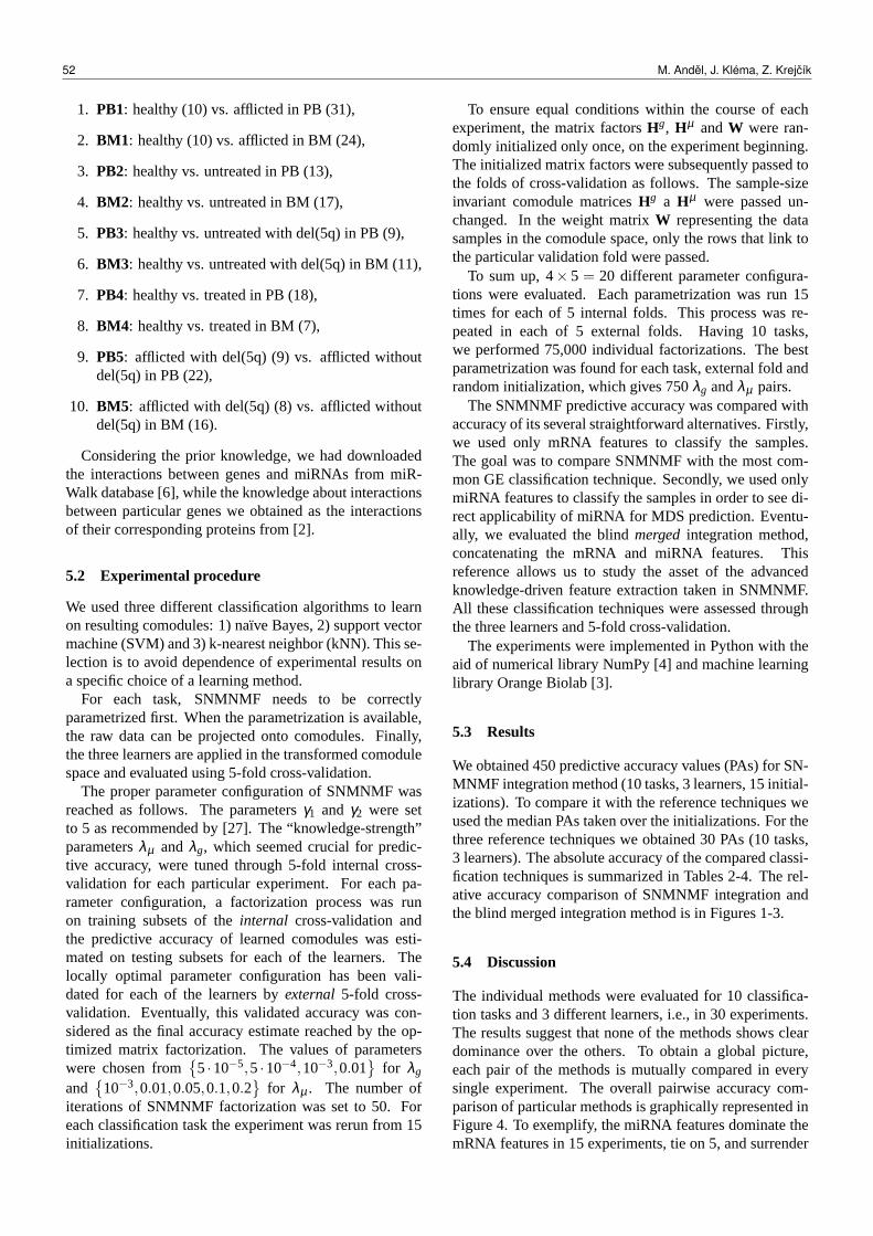
1. PB1: healthy (10) vs. afflicted in PB (31),

2. BM1: healthy (10) vs. afflicted in BM (24),

3. PB2: healthy vs. untreated in PB (13),

4. BM2: healthy vs. untreated in BM (17),

5. PB3: healthy vs. untreated with del(5q) in PB (9),

6. BM3: healthy vs. untreated with del(5q) in BM (11),

7. PB4: healthy vs. treated in PB (18),

8. BM4: healthy vs. treated in BM (7),

9. PB5: afflicted with del(5q) (9) vs. afflicted withoutdel(5q) in PB (22),

10. BM5: afflicted with del(5q) (8) vs. afflicted withoutdel(5q) in BM (16).

Considering the prior knowledge, we had downloadedthe interactions between genes and miRNAs from miR-Walk database [6], while the knowledge about interactionsbetween particular genes we obtained as the interactionsof their corresponding proteins from [2].

5.2 Experimental procedure

We used three different classification algorithms to learnon resulting comodules: 1) naïve Bayes, 2) support vectormachine (SVM) and 3) k-nearest neighbor (kNN). This se-lection is to avoid dependence of experimental results ona specific choice of a learning method.

For each task, SNMNMF needs to be correctlyparametrized first. When the parametrization is available,the raw data can be projected onto comodules. Finally,the three learners are applied in the transformed comodulespace and evaluated using 5-fold cross-validation.

The proper parameter configuration of SNMNMF wasreached as follows. The parametersγ1 and γ2 were setto 5 as recommended by [27]. The “knowledge-strength”parametersλµ andλg, which seemed crucial for predic-tive accuracy, were tuned through 5-fold internal cross-validation for each particular experiment. For each pa-rameter configuration, a factorization process was runon training subsets of theinternal cross-validation andthe predictive accuracy of learned comodules was esti-mated on testing subsets for each of the learners. Thelocally optimal parameter configuration has been vali-dated for each of the learners byexternal5-fold cross-validation. Eventually, this validated accuracy was con-sidered as the final accuracy estimate reached by the op-timized matrix factorization. The values of parameterswere chosen from

5·10−5,5·10−4,10−3,0.01

for λg

and

10−3,0.01,0.05,0.1,0.2

for λµ . The number ofiterations of SNMNMF factorization was set to 50. Foreach classification task the experiment was rerun from 15initializations.

To ensure equal conditions within the course of eachexperiment, the matrix factorsHg, Hµ andW were ran-domly initialized only once, on the experiment beginning.The initialized matrix factors were subsequently passed tothe folds of cross-validation as follows. The sample-sizeinvariant comodule matricesHg a Hµ were passed un-changed. In the weight matrixW representing the datasamples in the comodule space, only the rows that link tothe particular validation fold were passed.

To sum up, 4× 5 = 20 different parameter configura-tions were evaluated. Each parametrization was run 15times for each of 5 internal folds. This process was re-peated in each of 5 external folds. Having 10 tasks,we performed 75,000 individual factorizations. The bestparametrization was found for each task, external fold andrandom initialization, which gives 750λg andλµ pairs.

The SNMNMF predictive accuracy was compared withaccuracy of its several straightforward alternatives. Firstly,we used only mRNA features to classify the samples.The goal was to compare SNMNMF with the most com-mon GE classification technique. Secondly, we used onlymiRNA features to classify the samples in order to see di-rect applicability of miRNA for MDS prediction. Eventu-ally, we evaluated the blindmergedintegration method,concatenating the mRNA and miRNA features. Thisreference allows us to study the asset of the advancedknowledge-driven feature extraction taken in SNMNMF.All these classification techniques were assessed throughthe three learners and 5-fold cross-validation.

The experiments were implemented in Python with theaid of numerical library NumPy [4] and machine learninglibrary Orange Biolab [3].

5.3 Results

We obtained 450 predictive accuracy values (PAs) for SN-MNMF integration method (10 tasks, 3 learners, 15 initial-izations). To compare it with the reference techniques weused the median PAs taken over the initializations. For thethree reference techniques we obtained 30 PAs (10 tasks,3 learners). The absolute accuracy of the compared classi-fication techniques is summarized in Tables 2-4. The rel-ative accuracy comparison of SNMNMF integration andthe blind merged integration method is in Figures 1-3.

5.4 Discussion

The individual methods were evaluated for 10 classifica-tion tasks and 3 different learners, i.e., in 30 experiments.The results suggest that none of the methods shows cleardominance over the others. To obtain a global picture,each pair of the methods is mutually compared in everysingle experiment. The overall pairwise accuracy com-parison of particular methods is graphically represented inFigure 4. To exemplify, the miRNA features dominate themRNA features in 15 experiments, tie on 5, and surrender

52 M. Andel, J. Kléma, Z. Krejcík

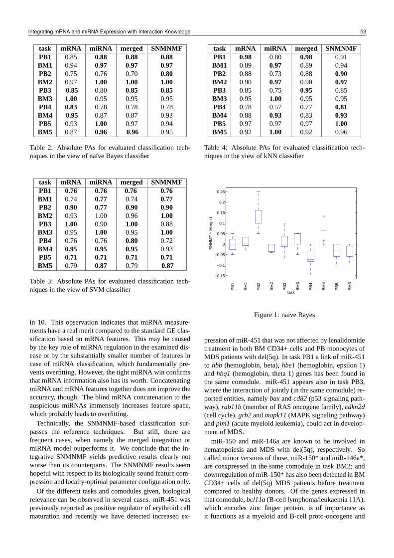
task mRNA miRNA merged SNMNMFPB1 0.85 0.88 0.88 0.88BM1 0.94 0.97 0.97 0.97PB2 0.75 0.76 0.70 0.80BM2 0.97 1.00 1.00 1.00PB3 0.85 0.80 0.85 0.85BM3 1.00 0.95 0.95 0.95PB4 0.83 0.78 0.78 0.78BM4 0.95 0.87 0.87 0.93PB5 0.93 1.00 0.97 0.94BM5 0.87 0.96 0.96 0.95

Table 2: Absolute PAs for evaluated classification tech-niques in the view of naïve Bayes classifier

task mRNA miRNA merged SNMNMFPB1 0.76 0.76 0.76 0.76BM1 0.74 0.77 0.74 0.77PB2 0.90 0.77 0.90 0.90BM2 0.93 1.00 0.96 1.00PB3 1.00 0.90 1.00 0.88BM3 0.95 1.00 0.95 1.00PB4 0.76 0.76 0.80 0.72BM4 0.95 0.95 0.95 0.93PB5 0.71 0.71 0.71 0.71BM5 0.79 0.87 0.79 0.87

Table 3: Absolute PAs for evaluated classification tech-niques in the view of SVM classifier

in 10. This observation indicates that miRNA measure-ments have a real merit compared to the standard GE clas-sification based on mRNA features. This may be causedby the key role of miRNA regulation in the examined dis-ease or by the substantially smaller number of features incase of miRNA classification, which fundamentally pre-vents overfitting. However, the tight miRNA win confirmsthat mRNA information also has its worth. ConcatenatingmiRNA and mRNA features together does not improve theaccuracy, though. The blind mRNA concatenation to theauspicious miRNAs immensely increases feature space,which probably leads to overfitting.

Technically, the SNMNMF-based classification sur-passes the reference techniques. But still, there arefrequent cases, when namely the merged integration ormiRNA model outperforms it. We conclude that the in-tegrative SNMNMF yields predictive results clearly notworse than its counterparts. The SNMNMF results seemhopeful with respect to its biologically sound feature com-pression and locally-optimal parameter configuration only.

Of the different tasks and comodules given, biologicalrelevance can be observed in several cases. miR-451 waspreviously reported as positive regulator of erythroid cellmaturation and recently we have detected increased ex-

task mRNA miRNA merged SNMNMFPB1 0.98 0.80 0.98 0.91BM1 0.89 0.97 0.89 0.94PB2 0.88 0.73 0.88 0.90BM2 0.90 0.97 0.90 0.97PB3 0.85 0.75 0.95 0.85BM3 0.95 1.00 0.95 0.95PB4 0.78 0.57 0.77 0.81BM4 0.88 0.93 0.83 0.93PB5 0.97 0.97 0.97 1.00BM5 0.92 1.00 0.92 0.96

Table 4: Absolute PAs for evaluated classification tech-niques in the view of kNN classifier

−0.15

−0.1

−0.05

0

0.05

0.1

0.15

0.2

0.25

PB

1

BM

1

PB

2

BM

2

PB

3

BM

3

PB

4

BM

4

PB

5

BM

5

task

SN

NM

F −

Mer

ged

Figure 1: naïve Bayes

pression of miR-451 that was not affected by lenalidomidetreatment in both BM CD34+ cells and PB monocytes ofMDS patients with del(5q). In task PB1 a link of miR-451to hbb (hemoglobin, beta),hbe1(hemoglobin, epsilon 1)andhbq1 (hemoglobin, theta 1) genes has been found inthe same comodule. miR-451 appears also in task PB3,where the interaction of jointly (in the same comodule) re-ported entities, namelybaxandcd82(p53 signaling path-way), rab11b(member of RAS oncogene family),cdkn2d(cell cycle),grb2andmapk11(MAPK signaling pathway)andpim1 (acute myeloid leukemia), could act in develop-ment of MDS.

miR-150 and miR-146a are known to be involved inhematopoiesis and MDS with del(5q), respectively. Socalled minor versions of those, miR-150* and miR-146a*,are coexpressed in the same comodule in task BM2; anddownregulation of miR-150* has also been detected in BMCD34+ cells of del(5q) MDS patients before treatmentcompared to healthy donors. Of the genes expressed inthat comodule,bcl11a(B-cell lymphoma/leukaemia 11A),which encodes zinc finger protein, is of importance asit functions as a myeloid and B-cell proto-oncogene and

Integrating mRNA and miRNA Expression with Interaction Knowledge 53

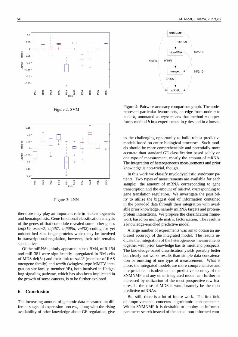
−0.25

−0.2

−0.15

−0.1

−0.05

0

0.05

0.1P

B1

BM

1

PB

2

BM

2

PB

3

BM

3

PB

4

BM

4

PB

5

BM

5

task

SN

NM

F −

Mer

ge

Figure 2: SVM

−0.2

−0.15

−0.1

−0.05

0

0.05

0.1

0.15

PB

1

BM

1

PB

2

BM

2

PB

3

BM

3

PB

4

BM

4

PB

5

BM

5

task

SN

NM

F −

Mer

ged

Figure 3: kNN

therefore may play an important role in leukaemogenesisand hematopoiesis. Gene functional classification analysisof the genes of that comodule revealed some other genes(znf319, zscan2, znf467, znf585a, znf32) coding for yetunidentified zinc finger proteins which may be involvedin transcriptional regulation, however, their role remainsspeculative.

Of the miRNAs jointly appeared in task BM4, miR-154and miR-381 were significantly upregulated in BM cellsof MDS del(5q) and their link torab23 (member of RASoncogene family) andwnt9b(wingless-type MMTV inte-gration site family, member 9B), both involved in Hedge-hog signaling pathway, which has also been implicated inthe growth of some cancers, is to be further explored.

6 Conclusion

The increasing amount of genomic data measured on dif-ferent stages of expression process, along with the risingavailability of prior knowledge about GE regulation, give

Figure 4: Pairwise accuracy comparison graph. The nodesrepresent particular feature sets, an edge from nodea tonodeb, annotated asx/y/z means that methoda outper-forms methodb in x experiments, iny ties and inz looses.

us the challenging opportunity to build robust predictivemodels based on entire biological processes. Such mod-els should be more comprehensible and potentially moreaccurate than standard GE classification based solely onone type of measurement, mostly the amount of mRNA.The integration of heterogeneous measurements and priorknowledge is non-trivial, though.

In this work we classify myelodysplastic syndrome pa-tients. Two types of measurements are available for eachsample: the amount of mRNA corresponding to genetranscription and the amount of miRNA corresponding togene translation regulation. We investigate the possibil-ity to utilize the biggest deal of information containedin the provided data through their integration with avail-able prior knowledge, namely miRNA targets and protein-protein interactions. We propose the classification frame-work based on multiple matrix factorization. The result isa knowledge-enriched predictive model.

A large number of experiments was run to obtain an un-biased accuracy of the integrated model. The results in-dicate that integration of the heterogeneous measurementstogether with prior knowledge has its merit and prospects.The knowledge-based classification yields possibly betterbut clearly not worse results than simple data concatena-tion or omitting of one type of measurement. What ismore, the integrated models are more comprehensive andinterpretable. It is obvious that predictive accuracy of theSNMNMF and any other integrated model can further beincreased by utilization of the most prospective raw fea-tures, in the case of MDS it would namely be the mostpredictive miRNAs.

But still, there is a lot of future work. The first fieldof improvements concerns algorithmic enhancements.Within SNMNMF it is desirable to employ an informedparameter search instead of the actual non-informed com-

54 M. Andel, J. Kléma, Z. Krejcík

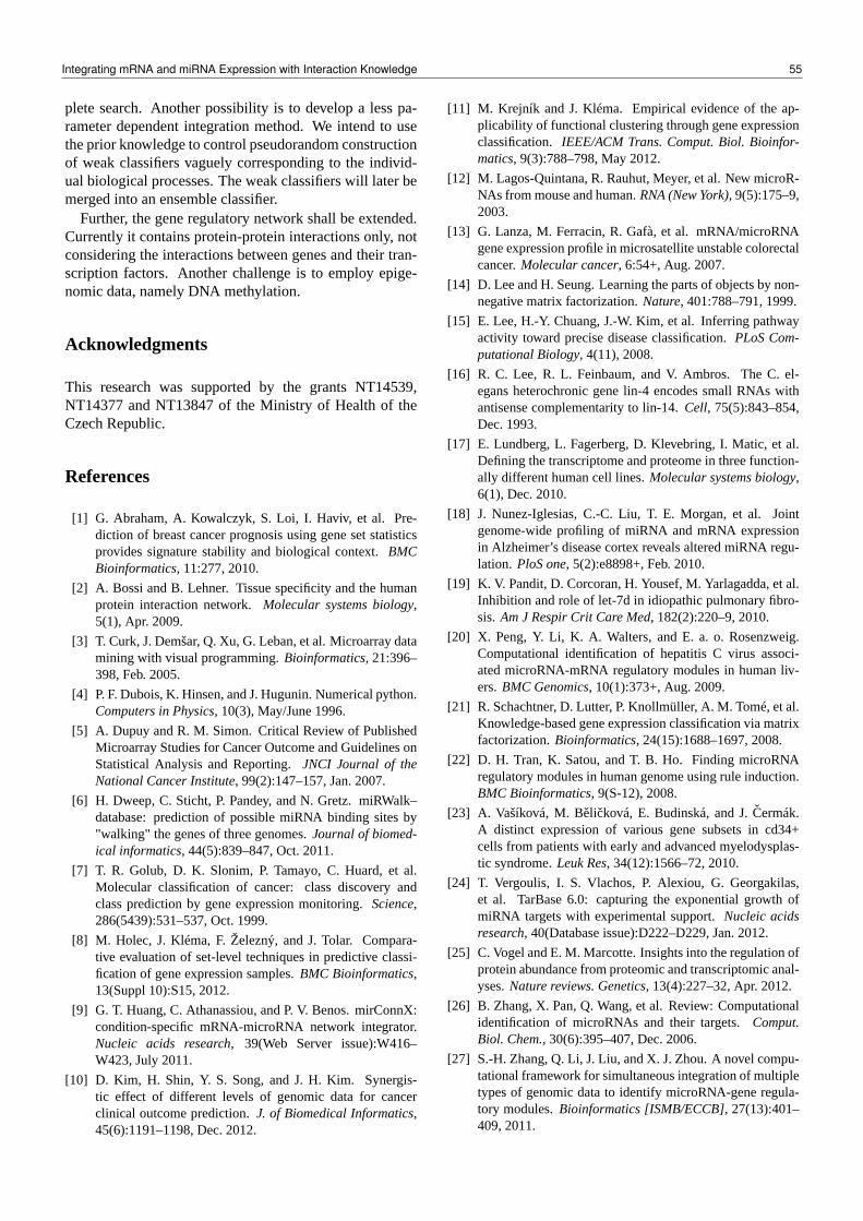
plete search. Another possibility is to develop a less pa-rameter dependent integration method. We intend to usethe prior knowledge to control pseudorandom constructionof weak classifiers vaguely corresponding to the individ-ual biological processes. The weak classifiers will later bemerged into an ensemble classifier.

Further, the gene regulatory network shall be extended.Currently it contains protein-protein interactions only,notconsidering the interactions between genes and their tran-scription factors. Another challenge is to employ epige-nomic data, namely DNA methylation.

Acknowledgments

This research was supported by the grants NT14539,NT14377 and NT13847 of the Ministry of Health of theCzech Republic.

References

[1] G. Abraham, A. Kowalczyk, S. Loi, I. Haviv, et al. Pre-diction of breast cancer prognosis using gene set statisticsprovides signature stability and biological context.BMCBioinformatics, 11:277, 2010.

[2] A. Bossi and B. Lehner. Tissue specificity and the humanprotein interaction network.Molecular systems biology,5(1), Apr. 2009.

[3] T. Curk, J. Demšar, Q. Xu, G. Leban, et al. Microarray datamining with visual programming.Bioinformatics, 21:396–398, Feb. 2005.

[4] P. F. Dubois, K. Hinsen, and J. Hugunin. Numerical python.Computers in Physics, 10(3), May/June 1996.

[5] A. Dupuy and R. M. Simon. Critical Review of PublishedMicroarray Studies for Cancer Outcome and Guidelines onStatistical Analysis and Reporting.JNCI Journal of theNational Cancer Institute, 99(2):147–157, Jan. 2007.

[6] H. Dweep, C. Sticht, P. Pandey, and N. Gretz. miRWalk–database: prediction of possible miRNA binding sites by"walking" the genes of three genomes.Journal of biomed-ical informatics, 44(5):839–847, Oct. 2011.

[7] T. R. Golub, D. K. Slonim, P. Tamayo, C. Huard, et al.Molecular classification of cancer: class discovery andclass prediction by gene expression monitoring.Science,286(5439):531–537, Oct. 1999.

[8] M. Holec, J. Kléma, F. Železný, and J. Tolar. Compara-tive evaluation of set-level techniques in predictive classi-fication of gene expression samples.BMC Bioinformatics,13(Suppl 10):S15, 2012.

[9] G. T. Huang, C. Athanassiou, and P. V. Benos. mirConnX:condition-specific mRNA-microRNA network integrator.Nucleic acids research, 39(Web Server issue):W416–W423, July 2011.

[10] D. Kim, H. Shin, Y. S. Song, and J. H. Kim. Synergis-tic effect of different levels of genomic data for cancerclinical outcome prediction.J. of Biomedical Informatics,45(6):1191–1198, Dec. 2012.

[11] M. Krejník and J. Kléma. Empirical evidence of the ap-plicability of functional clustering through gene expressionclassification. IEEE/ACM Trans. Comput. Biol. Bioinfor-matics, 9(3):788–798, May 2012.

[12] M. Lagos-Quintana, R. Rauhut, Meyer, et al. New microR-NAs from mouse and human.RNA (New York), 9(5):175–9,2003.

[13] G. Lanza, M. Ferracin, R. Gafà, et al. mRNA/microRNAgene expression profile in microsatellite unstable colorectalcancer.Molecular cancer, 6:54+, Aug. 2007.

[14] D. Lee and H. Seung. Learning the parts of objects by non-negative matrix factorization.Nature, 401:788–791, 1999.

[15] E. Lee, H.-Y. Chuang, J.-W. Kim, et al. Inferring pathwayactivity toward precise disease classification.PLoS Com-putational Biology, 4(11), 2008.

[16] R. C. Lee, R. L. Feinbaum, and V. Ambros. The C. el-egans heterochronic gene lin-4 encodes small RNAs withantisense complementarity to lin-14.Cell, 75(5):843–854,Dec. 1993.

[17] E. Lundberg, L. Fagerberg, D. Klevebring, I. Matic, et al.Defining the transcriptome and proteome in three function-ally different human cell lines.Molecular systems biology,6(1), Dec. 2010.

[18] J. Nunez-Iglesias, C.-C. Liu, T. E. Morgan, et al. Jointgenome-wide profiling of miRNA and mRNA expressionin Alzheimer’s disease cortex reveals altered miRNA regu-lation. PloS one, 5(2):e8898+, Feb. 2010.

[19] K. V. Pandit, D. Corcoran, H. Yousef, M. Yarlagadda, et al.Inhibition and role of let-7d in idiopathic pulmonary fibro-sis. Am J Respir Crit Care Med, 182(2):220–9, 2010.

[20] X. Peng, Y. Li, K. A. Walters, and E. a. o. Rosenzweig.Computational identification of hepatitis C virus associ-ated microRNA-mRNA regulatory modules in human liv-ers.BMC Genomics, 10(1):373+, Aug. 2009.

[21] R. Schachtner, D. Lutter, P. Knollmüller, A. M. Tomé, et al.Knowledge-based gene expression classification via matrixfactorization.Bioinformatics, 24(15):1688–1697, 2008.

[22] D. H. Tran, K. Satou, and T. B. Ho. Finding microRNAregulatory modules in human genome using rule induction.BMC Bioinformatics, 9(S-12), 2008.

[23] A. Vašíková, M. Belicková, E. Budinská, and J.Cermák.A distinct expression of various gene subsets in cd34+cells from patients with early and advanced myelodysplas-tic syndrome.Leuk Res, 34(12):1566–72, 2010.

[24] T. Vergoulis, I. S. Vlachos, P. Alexiou, G. Georgakilas,et al. TarBase 6.0: capturing the exponential growth ofmiRNA targets with experimental support.Nucleic acidsresearch, 40(Database issue):D222–D229, Jan. 2012.

[25] C. Vogel and E. M. Marcotte. Insights into the regulation ofprotein abundance from proteomic and transcriptomic anal-yses.Nature reviews. Genetics, 13(4):227–32, Apr. 2012.

[26] B. Zhang, X. Pan, Q. Wang, et al. Review: Computationalidentification of microRNAs and their targets.Comput.Biol. Chem., 30(6):395–407, Dec. 2006.

[27] S.-H. Zhang, Q. Li, J. Liu, and X. J. Zhou. A novel compu-tational framework for simultaneous integration of multipletypes of genomic data to identify microRNA-gene regula-tory modules.Bioinformatics [ISMB/ECCB], 27(13):401–409, 2011.

Integrating mRNA and miRNA Expression with Interaction Knowledge 55

Topology Incorporating Pathway Analysis of Expression Data: An Evaluationof Existing Methods

Ivana Ihnatova1

Bioinformatics In Translational Research Team, Institute of Biostatistics and Analyses, Brno, Czech Republic,WWW home page: http://btr.iba.muni.cz ihnatova@iba.muni.cz,

Abstract: Pathway analysis of expression data aims toassess the overall evidence of association of a biologicalpathway with a binary phenotype. Recently, a new ap-proach for this type of analysis has been proposed. Thesemethods use pathway topology to compute pathway-levelstatistics. Seven such methods are reviewed and comparedtheir performance via an extensive simulation study, inwhich the scenarios vary according to: the proportion ofdifferentially expressed genes, effect sizes and the loca-tion of the differentially expressed genes in the pathwaytopology.

The results demonstrate that Pathway regulation score,TopologyGSA and SPIA have the highest power for sce-narios with small proportion of the differentially expressedgenes. On the other hand, when the proportion of differen-tially expressed genes is high, TAPPA and DEGraph out-perform the other methods. TopologyGSA and Pathwayregulation score are the least sensitive to the positions ofdifferentially expressed genes in the pathway.

1 Introduction

Gene expression microarrays are a popular tool for detect-ing differences in gene activity across biological samples.Analysis of microarray data typically yields a list of differ-entially expressed genes. This list is extremely useful inidentifying genes that may have a role in given phenotype.However, biological processes are generally the result ofinteractions between multiple genes (pathways). To facil-itate such analyses, statistical methods have been devel-oped which focus on detecting changes in groups in func-tionally related genes, thus allowing additional biologicalinformation to be incorporated into the analysis process.This approach is called pathway analysis and the result ofit is a list of differentially expressed pathways.

An increasing number of publicly available databases(KEGG, Biocarta, Reactome, PID) provide not only a sim-ple lists of genes for each pathway, but also the interac-tions between them. Pathway topology (PT)-based meth-ods have been developed to utilize this additional infor-mation. PT-based methods were introduced in [1] andthey usually contain three steps: 1) calculation of gene-level statistics, 2) the gene-level statistics for all genes in apathway are aggregated into a single pathway level statis-tic (univariate or multivariate approaches), 3) assessing thestatistical significance of the pathway-level statistics (usu-ally by permutations).

Since PT-based methods are relatively new, a compara-tive review of them has not been published yet. The goalsof this paper are to describe the existing pathway topology-based methods and examine their performance through theanalysis of simulated data. Methods were selected accord-ing to their available implementation. For four out of sevenmethods there is a package available through Bioconduc-tor or CRAN. The remaining three methods were imple-mented in R by authors.

2 Material and Methods

2.1 Methods

In this section, the seven methods are briefly described.The phenotype of interest is assumed to be binary. Un-less stated otherwise, xis represents the expression valueof gene i in sample s and N denotes the number of genesin the pathway. A pathway is represented as directed graphG(V,E), V and E refer to set of nodes (vertices) and edges,respectively.

TAPPA TAPPA was introduced in [2]. The pathway-levelstatistic is called a Pathway Connectivity Index (PCI). Theindex is inspired by the second-order molecular connec-tivity index from chemoinformatics. The PCI is definedas

PCI =N

∑i=1

N

∑j=1

sgn(xis + x js)|xis|0.5ai j|x js|0.5,

where ai j = 1 if there is an edge between genes i and j andai j = 0 otherwise,xis denotes the expression value of gene iin sample s and sgn(xis+x js) represents the overall expres-sion status of the gene pair (up- or down-regulation). PCInormalized to the pathway size follow the normal distri-bution, therefore the Mann-Whitney test can be applied totest the hypothesis of equal medians of PCI in two groups.The pathway topology is incorportated as the higher con-tribution of the hub genes to PCI.

SPIA Signaling pathway impact analysis (SPIA) was de-veloped by Tarca et al. [3]. In the impact analysis, two in-dependent aspects of the pathway expression are capturedby two p-values PNDE and PPERT . The first one refers tothe significance of a pathway as provided by regular geneset analysis method (it is based on the number of DEG

ITAT 2013: Workshops, Posters, and Tutorials, pp. 56–61ISBN 978-1490952086, c© 2013 I. Ihnátová

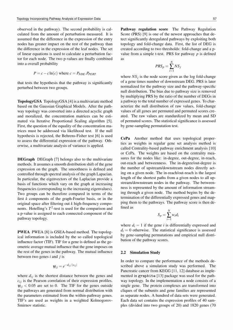
observed in the pathway). The second probability is cal-culated from the amount of perturbation measured. It isassumed that the difference in the expression of the entrynodes has greater impact on the rest of the pathway thanthe difference in the expression of the leaf nodes. The setof linear equations is used to calculate a perturbation fac-tor for each node. The two p-values are finally combinedinto a overall probability

P = c− c ln(c) where c = PNDE .PPERT

that tests the hypothesis that the pathway is significantlyperturbed between two groups.

TopologyGSA TopologyGSA [4] is a multivariate methodbased on the Gaussian Graphical Models. After the path-way topology was converted into a directed acyclic graphand moralized, the concentration matrices can be esti-mated via Iterative Proportional Scaling algorithm [5].First, the question of the equality of the concentration ma-trices must be addressed via likelihood test. If the nullhypothesis is rejected, the Behrens-Fisher test [6] is usedto assess the differential expression of the pathway. Oth-erwise, a multivariate analysis of variance is applied.

DEGraph DEGraph [7] belongs also to the multivariatemethods. It assumes a smooth distribution shift of the geneexpression on the graph. The smoothness is defined andcontrolled through spectral analysis of the graph Lapacian.In particular, the eigenvectors of the Laplacian provide abasis of functions which vary on the graph at increasingfrequencies (corresponding to the increasing eigenvalues).Two groups can be therefore compared in terms of thefirst k components of the graph-Fourier basis, or in theoriginal space after filtering out k high-frequency compo-nents. Hotelling’s T 2-test is used for the comparison anda p-value is assigned to each connected component of thepathway topology.

PWEA PWEA [8] is GSEA-based method. The topolog-ical information is included by the so called topologicalinfluence factor (TIF). TIF for a gene is defined as the ge-ometric average mutual influence that the gene imposes onthe rest of the genes in the pathway. The mutual influencebetween two genes i and j is

ψi j = e−di j/|ci j |

where di j is the shortest distance between the genes andci j is the Pearson correlation of their expression profiles.ψi j < 0.05 are set to 0. The TIF for the genes outsidethe pathways are generated from normal distribution withthe parameters estimated from the within-pathway genes.TIF’s are used as weights in a weighted Kolmogorov-Smirnov statistic.

Pathway regulation score The Pathway RegulationScore (PRS) [9] is one of the newest approaches that de-tect significantly deregulated pathways by exploiting bothtopology and fold-change data. First, the list of DEG iscreated according to two thresholds: fold-change and a p-value from a simple t-test. PRS for pathway p is definedas

PRSp =N

∑i=1

NS j

where NS j is the node score given as the log fold-changeof a gene times number of downstream DEG. PRS is laternormalized for the pathway size and the pathway-specificnull distribution. The bias due to pathway size is removedby multiplying PRS by the ratio of the number of DEGs ina pathway to the total number of expressed genes. To char-acterize the null distribution of raw values, fold-changevalues of all genes are permuted and permuted scores cre-ated. The raw values are standardized by mean and SDof permuted scores. The statistical significance is assessedby gene-sampling permutation test.

CePa Another method that uses topological proper-ties as weights in regular gene set analysis method iscalled Centrality-based pathway enrichment analysis [10]or CePa. The weights are based on the centrality mea-sures for the nodes like: in-degree, out-degree, in-reach,out-reach and betweenness. The in-degree/out-degree isthe number of upstream/downstream nodes directly act-ing on a given node. The in-reach/out-reach is the largestlength of the shortest paths from a given nodes to all up-stream/downstream nodes in the pathway. The between-ness is represented by the amount of information stream-ing through a given node. The method begins by the de-termination of the differentially expressed genes and map-ping them to the pathways. The pathway score is then de-fined as

Sp =N

∑i=1

widi

where di = 1 if the gene i is differentially expressed anddi = 0 otherwise. The statistical significance is assessedby gene-sampling permutations and empirical null distri-bution of the pathway scores.

2.2 Simulation Study

In order to compare the performance of the methods de-scribed above a simulation study was performed. ThePancreatic cancer from KEGG [11, 12] database as imple-mented in graphite [13] package was used for the path-way topology. In the implementation a node consists of asingle gene. The protein complexes are transformed intocliques of the subunits and gene families are representedas separate nodes. A hundred of data sets were generated.Each data set contains the expression profiles of 40 sam-ples (divided into two groups of 20) and 1820 genes (70

Topology Incorporating Pathway Analysis of Expression Data 57

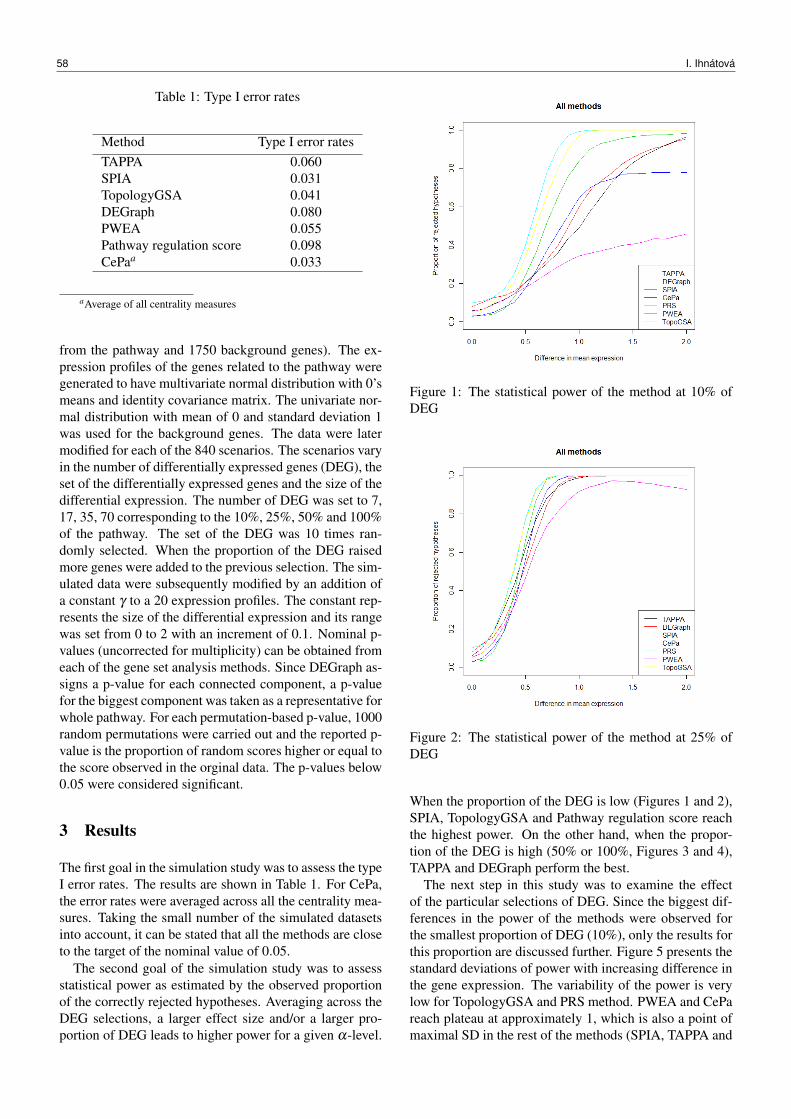
Table 1: Type I error rates

Method Type I error ratesTAPPA 0.060SPIA 0.031TopologyGSA 0.041DEGraph 0.080PWEA 0.055Pathway regulation score 0.098CePaa 0.033

aAverage of all centrality measures

from the pathway and 1750 background genes). The ex-pression profiles of the genes related to the pathway weregenerated to have multivariate normal distribution with 0’smeans and identity covariance matrix. The univariate nor-mal distribution with mean of 0 and standard deviation 1was used for the background genes. The data were latermodified for each of the 840 scenarios. The scenarios varyin the number of differentially expressed genes (DEG), theset of the differentially expressed genes and the size of thedifferential expression. The number of DEG was set to 7,17, 35, 70 corresponding to the 10%, 25%, 50% and 100%of the pathway. The set of the DEG was 10 times ran-domly selected. When the proportion of the DEG raisedmore genes were added to the previous selection. The sim-ulated data were subsequently modified by an addition ofa constant γ to a 20 expression profiles. The constant rep-resents the size of the differential expression and its rangewas set from 0 to 2 with an increment of 0.1. Nominal p-values (uncorrected for multiplicity) can be obtained fromeach of the gene set analysis methods. Since DEGraph as-signs a p-value for each connected component, a p-valuefor the biggest component was taken as a representative forwhole pathway. For each permutation-based p-value, 1000random permutations were carried out and the reported p-value is the proportion of random scores higher or equal tothe score observed in the orginal data. The p-values below0.05 were considered significant.

3 Results

The first goal in the simulation study was to assess the typeI error rates. The results are shown in Table 1. For CePa,the error rates were averaged across all the centrality mea-sures. Taking the small number of the simulated datasetsinto account, it can be stated that all the methods are closeto the target of the nominal value of 0.05.

The second goal of the simulation study was to assessstatistical power as estimated by the observed proportionof the correctly rejected hypotheses. Averaging across theDEG selections, a larger effect size and/or a larger pro-portion of DEG leads to higher power for a given α-level.

Figure 1: The statistical power of the method at 10% ofDEG

Figure 2: The statistical power of the method at 25% ofDEG

When the proportion of the DEG is low (Figures 1 and 2),SPIA, TopologyGSA and Pathway regulation score reachthe highest power. On the other hand, when the propor-tion of the DEG is high (50% or 100%, Figures 3 and 4),TAPPA and DEGraph perform the best.

The next step in this study was to examine the effectof the particular selections of DEG. Since the biggest dif-ferences in the power of the methods were observed forthe smallest proportion of DEG (10%), only the results forthis proportion are discussed further. Figure 5 presents thestandard deviations of power with increasing difference inthe gene expression. The variability of the power is verylow for TopologyGSA and PRS method. PWEA and CePareach plateau at approximately 1, which is also a point ofmaximal SD in the rest of the methods (SPIA, TAPPA and

58 I. Ihnátová

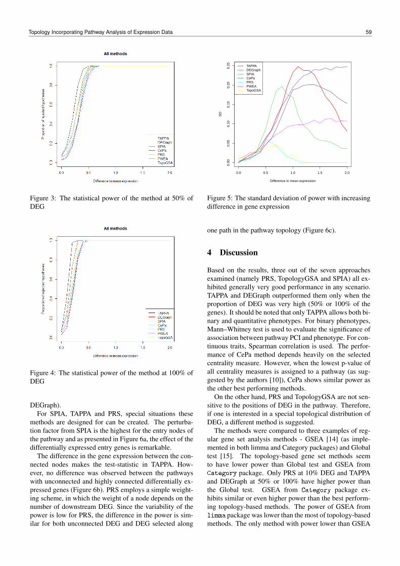
Figure 3: The statistical power of the method at 50% ofDEG

Figure 4: The statistical power of the method at 100% ofDEG

DEGraph).For SPIA, TAPPA and PRS, special situations these

methods are designed for can be created. The perturba-tion factor from SPIA is the highest for the entry nodes ofthe pathway and as presented in Figure 6a, the effect of thedifferentially expressed entry genes is remarkable.

The difference in the gene expression between the con-nected nodes makes the test-statistic in TAPPA. How-ever, no difference was observed between the pathwayswith unconnected and highly connected differentially ex-pressed genes (Figure 6b). PRS employs a simple weight-ing scheme, in which the weight of a node depends on thenumber of downstream DEG. Since the variability of thepower is low for PRS, the difference in the power is sim-ilar for both unconnected DEG and DEG selected along

0.0 0.5 1.0 1.5 2.0

0.00

0.05

0.10

0.15

0.20

0.25

Difference in mean expression

SD

TAPPADEGraphSPIACePaPRSPWEATopoGSA

Figure 5: The standard deviation of power with increasingdifference in gene expression

one path in the pathway topology (Figure 6c).

4 Discussion

Based on the results, three out of the seven approachesexamined (namely PRS, TopologyGSA and SPIA) all ex-hibited generally very good performance in any scenario.TAPPA and DEGraph outperformed them only when theproportion of DEG was very high (50% or 100% of thegenes). It should be noted that only TAPPA allows both bi-nary and quantitative phenotypes. For binary phenotypes,Mann–Whitney test is used to evaluate the significance ofassociation between pathway PCI and phenotype. For con-tinuous traits, Spearman correlation is used. The perfor-mance of CePa method depends heavily on the selectedcentrality measure. However, when the lowest p-value ofall centrality measures is assigned to a pathway (as sug-gested by the authors [10]), CePa shows similar power asthe other best performing methods.

On the other hand, PRS and TopologyGSA are not sen-sitive to the positions of DEG in the pathway. Therefore,if one is interested in a special topological distribution ofDEG, a different method is suggested.

The methods were compared to three examples of reg-ular gene set analysis methods - GSEA [14] (as imple-mented in both limma and Category packages) and Globaltest [15]. The topology-based gene set methods seemto have lower power than Global test and GSEA fromCategory package. Only PRS at 10% DEG and TAPPAand DEGraph at 50% or 100% have higher power thanthe Global test. GSEA from Category package ex-hibits similar or even higher power than the best perform-ing topology-based methods. The power of GSEA fromlimma package was lower than the most of topology-basedmethods. The only method with power lower than GSEA

Topology Incorporating Pathway Analysis of Expression Data 59

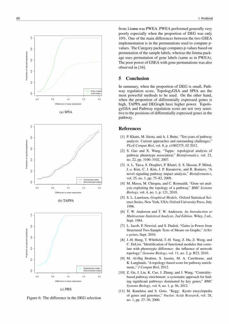
0.0 0.5 1.0 1.5 2.0

0.0

0.2

0.4

0.6

0.8

1.0

Difference in mean expression

Pro

port

ion

of r

ejec

ted

hypo

thes

es

Entry nodesLeaf nodes

(a) SPIA

0.0 0.5 1.0 1.5 2.0

0.0

0.2

0.4

0.6

0.8

1.0

Difference in mean expression

Pro

port

ion

of r

ejec

ted

hypo

thes

es

Connected nodesDisconnected nodes

(b) TAPPA

0.0 0.5 1.0 1.5 2.0

0.0

0.2

0.4

0.6

0.8

1.0

Difference in mean expression

Pro

port

ion

of r

ejec

ted

hypo

thes

es

Downstream nodesDisconnected nodes

(c) PRS

Figure 6: The difference in the DEG selection

from limma was PWEA. PWEA performed generally verypoorly especially when the proportion of DEG was only10%. One of the main differences between the two GSEAimplementation is in the permutations used to compute p-values. The Category package computes p-values based onpermutation of the sample labels, whereas the limma pack-age uses permutation of gene labels (same as in PWEA).The poor power of GSEA with gene permutations was alsoobserved in [16].

5 ConclusionIn summary, when the proportion of DEG is small, Path-way regulation score, TopologyGSA and SPIA are themost powerful methods to be used. On the other hand,when the proportion of differentially expressed genes ishigh, TAPPA and DEGraph have higher power. Topolo-gyGSA and Pathway regulation score are not very sensi-tive to the positions of differentially expressed genes in thepathway.

References[1] P. Khatri, M. Sirota, and A. J. Butte, “Ten years of pathway

analysis: Current approaches and outstanding challenges,”PLoS Comput Biol, vol. 8, p. e1002375, 02 2012.

[2] S. Gao and X. Wang, “Tappa: topological analysis ofpathway phenotype association,” Bioinformatics, vol. 23,no. 22, pp. 3100–3102, 2007.

[3] A. L. Tarca, S. Draghici, P. Khatri, S. S. Hassan, P. Mittal,J.-s. Kim, C. J. Kim, J. P. Kusanovic, and R. Romero, “Anovel signaling pathway impact analysis,” Bioinformatics,vol. 25, no. 1, pp. 75–82, 2009.

[4] M. Massa, M. Chiogna, and C. Romualdi, “Gene set anal-ysis exploiting the topology of a pathway,” BMC SystemsBiology, vol. 4, no. 1, p. 121, 2010.

[5] S. L. Lauritzen, Graphical Models. Oxford Statistical Sci-ence Series, New York, USA: Oxford University Press, July1996.

[6] T. W. Anderson and T. W. Anderson, An Introduction toMultivariate Statistical Analysis, 2nd Edition. Wiley, 2 ed.,Sept. 1984.

[7] L. Jacob, P. Neuvial, and S. Dudoit, “Gains in Power fromStructured Two-Sample Tests of Means on Graphs,” ArXive-prints, Sept. 2010.

[8] J.-H. Hung, T. Whitfield, T.-H. Yang, Z. Hu, Z. Weng, andC. DeLisi, “Identification of functional modules that corre-late with phenotypic difference: the influence of networktopology,” Genome Biology, vol. 11, no. 2, p. R23, 2010.

[9] M. Al-Haj Ibrahim, S. Jassim, M. A. Cawthorne, andK. Langlands, “A topology-based score for pathway enrich-ment.,” J Comput Biol, 2012.

[10] Z. Gu, J. Liu, K. Cao, J. Zhang, and J. Wang, “Centrality-based pathway enrichment: a systematic approach for find-ing significant pathways dominated by key genes,” BMCSystems Biology, vol. 6, no. 1, p. 56, 2012.

[11] M. Kanehisa and S. Goto, “Kegg: Kyoto encyclopediaof genes and genomes,” Nucleic Acids Research, vol. 28,no. 1, pp. 27–30, 2000.

60 I. Ihnátová

[12] M. Kanehisa, S. Goto, Y. Sato, M. Furumichi, and M. Tan-abe, “Kegg for integration and interpretation of large-scalemolecular data sets,” Nucleic Acids Research, vol. 40,no. D1, pp. D109–D114, 2012.

[13] G. Sales, E. Calura, and C. Romualdi, graphite: GRAPHInteraction from pathway Topological Environment, 2013.R package version 1.6.0.

[14] A. Subramanian, P. Tamayo, V. K. Mootha, S. Mukherjee,B. L. Ebert, M. A. Gillette, A. Paulovich, S. L. Pomeroy,T. R. Golub, E. S. Lander, and J. P. Mesirov, “Gene setenrichment analysis: A knowledge-based approach for in-terpreting genome-wide expression profiles,” Proceedingsof the National Academy of Sciences of the United States ofAmerica, vol. 102, no. 43, pp. 15545–15550, 2005.

[15] J. J. Goeman, S. A. van de Geer, F. de Kort, and H. C. vanHouwelingen, “A global test for groups of genes: testing as-sociation with a clinical outcome,” Bioinformatics, vol. 20,no. 1, pp. 93–99, 2004.

[16] S. Song and M. Black, “Microarray-based gene set analy-sis: a comparison of current methods,” BMC Bioinformat-ics, vol. 9, no. 1, p. 502, 2008.

Topology Incorporating Pathway Analysis of Expression Data 61

Study of the receiver and receiver-like domain relationship in cytokinin receptor of Arabidopsis thaliana

Vendula Hrdinová

Functional genomics and proteomics of plants Central European Institute of Technology, Masaryk University

Kamenice 5/A2, CZ-625 00 Brno, Czech Republic

Blanka Pekárová, Tomáš Klumpler, Lubomír Janda, Jan Hejátko Functional genomics and proteomics of plants

Central European Institute of Technology, Masaryk University Kamenice 5/A2, CZ-625 00 Brno, Czech Republic

Abstract. Cytokinin (CK) signaling is one of the

pathways mediated by multistep phosphorelay (MSP) in plants. In the MSP of Arabidopsis thaliana, Arabidopsis histidine kinases (AHKs) act as receptors initiating the pathway and interact with Arabidopsis histidine-containing proteins (AHPs), thus transferring the signal farther in the cascade. For the signal transduction through the cascade, the domain composition of the MSP elements is crucial. Recently it was reported that the receiver domain of one of the Arabidopsis sensor histidine kinases CKI1 is sufficient and necessary for the specific interaction of CKI1 with AHPs. Here we performed an extensive study of the individual domains of CK receptor AHK4 in mediating interactions with AHPs. Thorough bioinformatic analysis of the AHK4 aa sequence using similarity search was carried out to refine the precise borders of AHK4 individual domains. SMART and PROSITE databases for primary and secondary structure analysis were used to identify similarities within receiver and receiver-like domains of other AHKs and the results were manually refined. Moreover, we modeled individual structures of the receiver and receiver-like domain of AHK4 (AHK4RD and AHK4RLD, respectively) employing their homology with solved structure of bacterial response regulator receiver domain CheY in order to see possible differences in the structure and to predict potential interaction interfaces. The structural predictions were used to design recombinant DNA constructs for protein-protein interaction experiments. Intriguingly, by yeast two-hybrid analysis we revealed that not only AHK4RD is substantial for the interaction with AHPs but we found out that the interaction can be suppressed by AHK4RLD. We propose that AHK4RLD

has a (negative) regulatory function in the process of molecular recognition of the downstream signaling partners and we experimentally demonstrated that this function can be provided by the heterodimerization of AHK4RD with AHK4RLD, either intra- or intermolecularly. The structural prediction-based model of this regulatory role will be presented.

Supported by the European Regional Development Fund

(Central European Institute of Technology project no. CZ.1.05/1.1.00/02.0068), the European Social Fund (CZ.1.07/2.3.00/20.0189) and the Czech Science Foundation (P305/11/0756).

ITAT 2013: Workshops, Posters, and Tutorials, p. 62ISBN 978-1490952086, c© 2013 V. Hrdinová, B. Pekárová, T. Klumpler, L. Janda, J. Hejátko

Elucidating molecular mechanisms of cytokinin action in the vascular bundle development of Arabidopsis thaliana

Vojtěch Didi

Functional Genomics and Proteomics of Plants CEITEC - Central European Institute of Technology, Masaryk University

Kamenice 5, 625 00 Brno, Czech Republic

Radim Čegan2, Mariana Benítez3, Tereza Dobisová1, Roman Hobza2, Vít Gloser4 and Jan Hejátko1

1 - Functional Genomics and Proteomics of Plants CEITEC - Central European Institute of Technology, Masaryk University

Kamenice 5, 625 00 Brno, Czech Republic

2 - Department of Plant Developmental Genetics Institute of Biophysics, The Academy of Sciences of the Czech Republic

Královopolská 135, 612 65 Brno, Czech Republic

3 - Instituto de Ecología Universidad Nacional Autónoma de México

Mexico

4 - Department of Experimental Biology Faculty of Science, Masaryk University

Kamenice 5, 625 00 Brno, Czech Republic

Cytokinins (CKs) belong to plant growth factors

(phytohormones) and participate in numerous physiological and developmental processes such as cell division, leaf senescence, vascular bundle pattering, apical dominance, lateral root formation, chloroplast development and regulation of meristematic tissues activity. CK signalling is ensured via multistep phosphorelay (MSP). The MSP signaling pathway consists of mostly membrane-located sensor histidine kinases (HKs), histidin phosphotransfer proteins (HPts), which transfer the signal to the nucleus and response regulators (RRs). Some of these RRs act as transcriptional factors and orchestrate expression of their target genes via direct binding to the promoter sequence or through indirect regulations.

Our results show that CKs play crucial role in development of vascular bundles (VBs). We found that downregulating CK signaling or depleting endogenous CK levels affected development of specific vascular cell types and their functional properties. To elucidate molecular mechanisms underlying CK-regulated vascular tissue development, we employed next-gen transcriptional profiling. Total RNA from the apical portion of inflorescence stem from the WT and CK signaling mutant was isolated, cDNA sequencing libraries (three biological replicas from each genotype) were prepared and sequenced by Ilumina technology (HiSeq 2000). The output data were analyzed by TopHat program and almost 7000 differentially expressed genes were identified. The subsequent analysis of gene ontology (GO) via Gorilla software (cbl-gorilla.cs.technion.ac.il/) allowed us to identify developmental processes that were dominantly affected in the CK signaling mutant. The resulting model

based on the aforementioned experimental and bioinformatic analyses and describing novel molecular mechanism of CK action in the vascular tissue development will be presented.

Supported by the European Regional Development Fund

(Central European Institute of Technology project no. CZ.1.05/1.1.00/02.0068), the European Social Fund (CZ.1.07/2.3.00/20.0189) and the Czech Science Foundation (13-25280S).

ITAT 2013: Workshops, Posters, and Tutorials, p. 63ISBN 978-1490952086, c© 2013 V. Didi, R. Cegan, M. Benítez, T. Dobisová, R. Hobza, V. Gloser, J. Hejátko

Generovanie simulovaných testovacích dát pre genómové asociacné štúdie

Stanislav Štefanic, Matej Lexa

Fakulta informatiky, Masaryková univerzita, Botanická 68a, 60200 Brno, Ceská republika, 374513@mail.muni.cz, lexa@fi.muni.cz

Abstrakt: V posledných rokoch zaznamenávame vo vý-skumoch l’udských chorôb prudký nárast genomovéhosekvenovania vzoriek jedincov a následne hromadnej de-tekcie genetických asociácií medzi variáciami (prevažneSNP mutácie) a presnou diagnózou. Tieto techniky vy-ústili do rutinného používania techník zvaných genómovéasociacné štúdia (GWAS 1). Jedná sa o štúdie, pri ktorýchhl’adáme asociácie medzi variáciami a fenotypom na ce-lom genóme jedincov. Detekovanie asociácie medzi jed-ným SNP a konkrétnou crtou jedinca sa dnes prevádza ru-tinne, no drvivá väcšina biologicky relevantných vzt’ahovzahrna interakciu viacerých SNP, ktoré súcasne asociujús danou fenotypovou crtou. Hl’adanie takýchto interakciíje však kamenom úrazu v GWA štúdiach. V súcasnos-ti sa snažíme tento problém vyriešit’ a hl’adáme možnostiako tieto interakcie odhal’ovat’. Pri testovaní metód a po-stupov, ktoré majú tieto a podobné interakcie a asociácieodhal’ovat’ je castým a jedným z najväcších problémov ne-dostatok reálnych dát, u ktorých máme informáciu o všet-kých neznámych vzt’ahoch. Preto je namieste používanieumelých testovacích dát. Zaznamenávame niekol’ko po-kusov o riešenie tohoto problému práve cestou generova-nia umelých dát, ich problém však spocíva v nedostatocnejzložitosti a možnosti presného priblíženia simulovanýchdát. Ciel’om našej práce je tieto nedostatky odstránit’ aposkytnút’ možnost’ generovat’ aj pomerne zložité simu-lované dáta s dostatocne presnou možnost’ou priblíženiatýchto dát reálnym dátam a vzt’ahom vyskytujúcim sa vprírode. Navrhnutá aplikácia poskytuje užívatel’ovi pre-hl’adné grafické užívatel’ské rozhranie v ktorom nastavujeradu parametrov na základe ktorých sa budú dáta gene-rovat’. Presné nastavenia korelácií jednotlivých mutácií(SNP) a frekvencií jednotlivých alel je definované užíva-tel’om zadanou funkciou, ktorá tieto parametre dostatoc-ne dobre popisuje. Výstupy tejto aplikácie boli testovanéna metódach, ktoré odhal’ujú skryté asociácie a interakciemedzi SNP navzájom a chorobou a ukryté vzt’ahy v tých-to dátach boli správne detekované. Fungovanie aplikácie avýsledky práce ilustrujeme.

1 Úvod

Genómy jednotlivých zástupcov l’udského druhu sú z99.9% rovnaké. Genóm každého jedinca reprezentuje ce-lú genetickú informáciu cloveka, zakódovanú ako postup-nost’ jednotlivých nukleotidových báz (A, C, T, G). Roz-diel medzi genetickými informáciami jednotlivých jedin-cov (0.1%) spôsobujú urcité variácie v genóme, nazývané

1Genome-wide association studies

mutácie. Tieto mutácie sú pre l’udský druh doležité jednakz hl’adiska evolúcie a vývoja nášho druhu (napr. tvorbaimunitného systému, adaptácia na zmeny životných pod-mienok) na druhej strane však spôsobujú defekty a rôzneanomálie u jednotlivých clenov populácie (genetické cho-roby). Pre oznacenie mutácií sa používajú pojmy poly-morfizmus a SNP. Za polymorfizmus považujeme mutácie,ktoré sú rovnaké aspon u jedného percenta zástupcov isté-ho druhu, poprípade skúmanej vzorky jedincov [1]. Špe-ciálny prípad polymorfizmu je taký, kedy uvažujeme lenbodové mutácie - mutácie na rovnakých pozíciach v po-stupnostiach báz jednotlivých individuí. V takomto prípa-de hovoríme o jednonukleotidovom polymorfizme, skrá-tene SNP [2]2. Zacali sa preto sekvenovat’ genetické in-formácie zástupcov populácie, identifikovat’ medzi nimiSNP, pozorovat’ fenotypové crty osekvenovaných l’udí adetekovat’ vzt’ahy medzi identifikovanými SNP a urcitoufenotypovou charakteristikou. Základnému výskumu po-lymorfizmov sa venujú vedecké projekty ako sú 1000ge-nomes [3]3, HAPMAP [4]4, vedecký inštitút NCBI [5]5 ainé. Najcastejším spôsobom skúmania vzt’ahu polymor-fizmov a fenotypov sú štúdia génových asociácií, z nich vdnešnej dobe najviac rozšírené sú GWA štúdie [6]. Jed-ná sa o prístup k štúdiu asociácií medzi SNP kedy uvažu-jeme mutácie v celom genóme, nie iba na urcitom blokualebo casti genómu. Osekvenované alebo inak identifiko-vané SNP sa pre d’alšie skúmanie ukladajú do súborov všpeciálnych formátoch, napríklad VCF [7]. Tieto metódypri dostatocnom množstve pacientov spol’ahlivo odhaliaasociáciu jedného SNP a fenotypu. Existuje podozrenie,že väcšina biologicky a medicínsky zaujímavých asociáciínám ostáva skrytá. Dôvodom je vel’ké množstvo mutá-cií, ktoré nepôsobia izolovane, ale v interakcii s d’alšímimutáciami. Známym príkladom takejto interakcie je epis-táza [8]. Postupom casu vznikali metódy, ktoré sa sna-žili tieto interakcie detekovat’, avšak dáta na ktorých bysa mali verifikovat’ casto chýbajú. Z toho dôvodu je zau-jímavé algoritmy testovat’ a porovnávat’ medzi sebou naumelých dátach, u ktorých máme informáciu o hl’adanýchvzt’ahoch.

1.1 Potreba umelých dát

Pre efektívne testovanie a porovnávanie GWAS algorit-mov je vhodné generovat’ simulované dáta potrebného ty-pu. Jedná sa o dáta vo formátoch VCF, poprípade MAP

2single nucleotide polymorphism3http://www.1000genomes.org/4http://hapmap.ncbi.nlm.nih.gov/5http://www.ncbi.nlm.nih.gov/

ITAT 2013: Workshops, Posters, and Tutorials, pp. 64–68ISBN 978-1490952086, c© 2013 S. Štefanic, M. Lexa

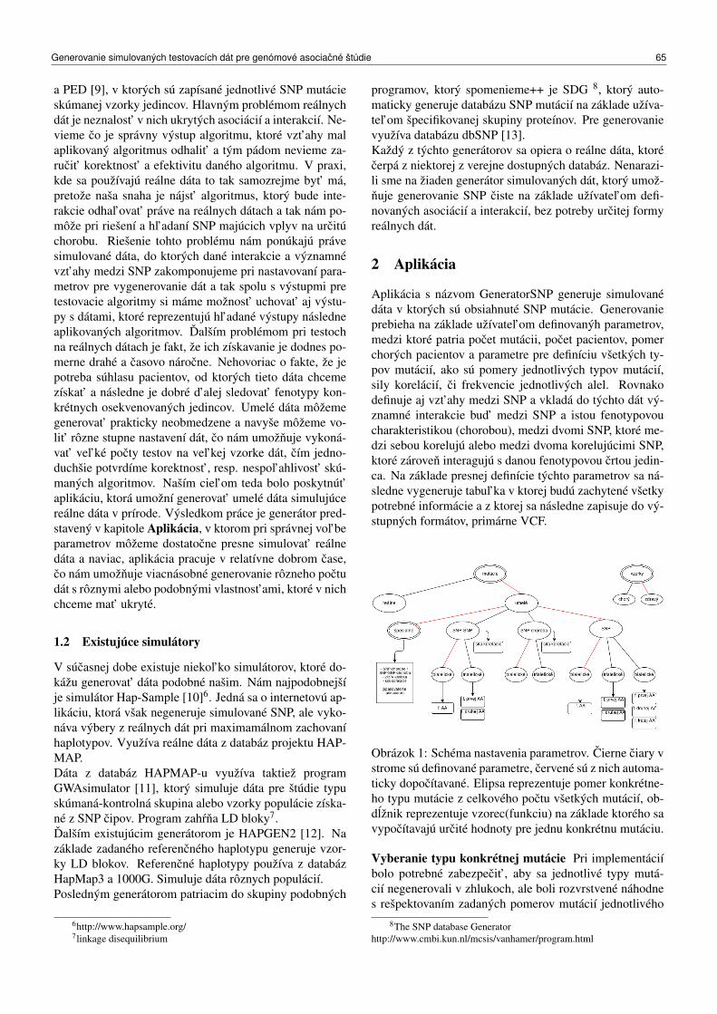
a PED [9], v ktorých sú zapísané jednotlivé SNP mutácieskúmanej vzorky jedincov. Hlavným problémom reálnychdát je neznalost’ v nich ukrytých asociácií a interakcií. Ne-vieme co je správny výstup algoritmu, ktoré vzt’ahy malaplikovaný algoritmus odhalit’ a tým pádom nevieme za-rucit’ korektnost’ a efektivitu daného algoritmu. V praxi,kde sa používajú reálne dáta to tak samozrejme byt’ má,pretože naša snaha je nájst’ algoritmus, ktorý bude inte-rakcie odhal’ovat’ práve na reálnych dátach a tak nám po-môže pri riešení a hl’adaní SNP majúcich vplyv na urcitúchorobu. Riešenie tohto problému nám ponúkajú právesimulované dáta, do ktorých dané interakcie a významnévzt’ahy medzi SNP zakomponujeme pri nastavovaní para-metrov pre vygenerovanie dát a tak spolu s výstupmi pretestovacie algoritmy si máme možnost’ uchovat’ aj výstu-py s dátami, ktoré reprezentujú hl’adané výstupy následneaplikovaných algoritmov. Dalším problémom pri testochna reálnych dátach je fakt, že ich získavanie je dodnes po-merne drahé a casovo nárocne. Nehovoriac o fakte, že jepotreba súhlasu pacientov, od ktorých tieto dáta chcemezískat’ a následne je dobré d’alej sledovat’ fenotypy kon-krétnych osekvenovaných jedincov. Umelé dáta môžemegenerovat’ prakticky neobmedzene a navyše môžeme vo-lit’ rôzne stupne nastavení dát, co nám umožnuje vykoná-vat’ vel’ké pocty testov na vel’kej vzorke dát, cím jedno-duchšie potvrdíme korektnost’, resp. nespol’ahlivost’ skú-maných algoritmov. Naším ciel’om teda bolo poskytnút’aplikáciu, ktorá umožní generovat’ umelé dáta simulujúcereálne dáta v prírode. Výsledkom práce je generátor pred-stavený v kapitole Aplikácia, v ktorom pri správnej vol’beparametrov môžeme dostatocne presne simulovat’ reálnedáta a naviac, aplikácia pracuje v relatívne dobrom case,co nám umožnuje viacnásobné generovanie rôzneho poctudát s rôznymi alebo podobnými vlastnost’ami, ktoré v nichchceme mat’ ukryté.

1.2 Existujúce simulátory

V súcasnej dobe existuje niekol’ko simulátorov, ktoré do-kážu generovat’ dáta podobné našim. Nám najpodobnejšíje simulátor Hap-Sample [10]6. Jedná sa o internetovú ap-likáciu, ktorá však negeneruje simulované SNP, ale vyko-náva výbery z reálnych dát pri maximamálnom zachovaníhaplotypov. Využíva reálne dáta z databáz projektu HAP-MAP.Dáta z databáz HAPMAP-u využíva taktiež programGWAsimulator [11], ktorý simuluje dáta pre štúdie typuskúmaná-kontrolná skupina alebo vzorky populácie získa-né z SNP cipov. Program zahrna LD bloky7.Dalším existujúcim generátorom je HAPGEN2 [12]. Nazáklade zadaného referencného haplotypu generuje vzor-ky LD blokov. Referencné haplotypy používa z databázHapMap3 a 1000G. Simuluje dáta rôznych populácií.Posledným generátorom patriacim do skupiny podobných

6http://www.hapsample.org/7linkage disequilibrium

programov, ktorý spomenieme++ je SDG 8, ktorý auto-maticky generuje databázu SNP mutácií na základe užíva-tel’om špecifikovanej skupiny proteínov. Pre generovanievyužíva databázu dbSNP [13].Každý z týchto generátorov sa opiera o reálne dáta, ktorécerpá z niektorej z verejne dostupných databáz. Nenarazi-li sme na žiaden generátor simulovaných dát, ktorý umož-nuje generovanie SNP ciste na základe užívatel’om defi-novaných asociácií a interakcií, bez potreby urcitej formyreálnych dát.

2 Aplikácia

Aplikácia s názvom GeneratorSNP generuje simulovanédáta v ktorých sú obsiahnuté SNP mutácie. Generovanieprebieha na základe užívatel’om definovanýh parametrov,medzi ktoré patria pocet mutácii, pocet pacientov, pomerchorých pacientov a parametre pre definíciu všetkých ty-pov mutácií, ako sú pomery jednotlivých typov mutácií,sily korelácií, ci frekvencie jednotlivých alel. Rovnakodefinuje aj vzt’ahy medzi SNP a vkladá do týchto dát vý-znamné interakcie bud’ medzi SNP a istou fenotypovoucharakteristikou (chorobou), medzi dvomi SNP, ktoré me-dzi sebou korelujú alebo medzi dvoma korelujúcimi SNP,ktoré zároven interagujú s danou fenotypovou crtou jedin-ca. Na základe presnej definície týchto parametrov sa ná-sledne vygeneruje tabul’ka v ktorej budú zachytené všetkypotrebné informácie a z ktorej sa následne zapisuje do vý-stupných formátov, primárne VCF.

Obrázok 1: Schéma nastavenia parametrov. Cierne ciary vstrome sú definované parametre, cervené sú z nich automa-ticky dopocítavané. Elipsa reprezentuje pomer konkrétne-ho typu mutácie z celkového poctu všetkých mutácií, ob-dlžnik reprezentuje vzorec(funkciu) na základe ktorého savypocítavajú urcité hodnoty pre jednu konkrétnu mutáciu.

Vyberanie typu konkrétnej mutácie Pri implementáciíbolo potrebné zabezpecit’, aby sa jednotlivé typy mutá-cií negenerovali v zhlukoch, ale boli rozvrstvené náhodnes rešpektovaním zadaných pomerov mutácií jednotlivého

8The SNP database Generatorhttp://www.cmbi.kun.nl/mcsis/vanhamer/program.html

Generovanie simulovaných testovacích dát pre genómové asociacné štúdie 65

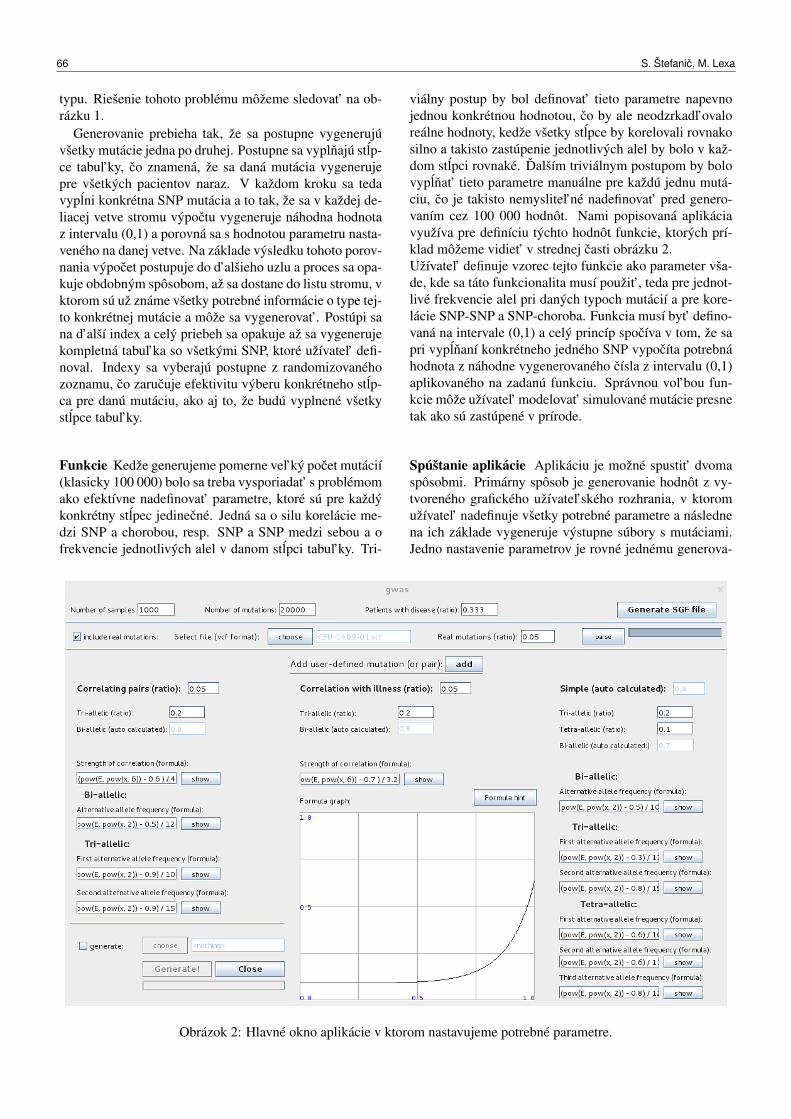
typu. Riešenie tohoto problému môžeme sledovat’ na ob-rázku 1.

Generovanie prebieha tak, že sa postupne vygenerujúvšetky mutácie jedna po druhej. Postupne sa vyplnajú stlp-ce tabul’ky, co znamená, že sa daná mutácia vygenerujepre všetkých pacientov naraz. V každom kroku sa tedavyplni konkrétna SNP mutácia a to tak, že sa v každej de-liacej vetve stromu výpoctu vygeneruje náhodna hodnotaz intervalu (0,1) a porovná sa s hodnotou parametru nasta-veného na danej vetve. Na základe výsledku tohoto porov-nania výpocet postupuje do d’alšieho uzlu a proces sa opa-kuje obdobným spôsobom, až sa dostane do listu stromu, vktorom sú už známe všetky potrebné informácie o type tej-to konkrétnej mutácie a môže sa vygenerovat’. Postúpi sana d’alší index a celý priebeh sa opakuje až sa vygenerujekompletná tabul’ka so všetkými SNP, ktoré užívatel’ defi-noval. Indexy sa vyberajú postupne z randomizovanéhozoznamu, co zarucuje efektivitu výberu konkrétneho stlp-ca pre danú mutáciu, ako aj to, že budú vyplnené všetkystlpce tabul’ky.

Funkcie Kedže generujeme pomerne vel’ký pocet mutácií(klasicky 100 000) bolo sa treba vysporiadat’ s problémomako efektívne nadefinovat’ parametre, ktoré sú pre každýkonkrétny stlpec jedinecné. Jedná sa o silu korelácie me-dzi SNP a chorobou, resp. SNP a SNP medzi sebou a ofrekvencie jednotlivých alel v danom stlpci tabul’ky. Tri-

viálny postup by bol definovat’ tieto parametre napevnojednou konkrétnou hodnotou, co by ale neodzrkadl’ovaloreálne hodnoty, kedže všetky stlpce by korelovali rovnakosilno a takisto zastúpenie jednotlivých alel by bolo v kaž-dom stlpci rovnaké. Dalším triviálnym postupom by bolovyplnat’ tieto parametre manuálne pre každú jednu mutá-ciu, co je takisto nemyslitel’né nadefinovat’ pred genero-vaním cez 100 000 hodnôt. Nami popisovaná aplikáciavyužíva pre definíciu týchto hodnôt funkcie, ktorých prí-klad môžeme vidiet’ v strednej casti obrázku 2.Užívatel’ definuje vzorec tejto funkcie ako parameter vša-de, kde sa táto funkcionalita musí použit’, teda pre jednot-livé frekvencie alel pri daných typoch mutácií a pre kore-lácie SNP-SNP a SNP-choroba. Funkcia musí byt’ defino-vaná na intervale (0,1) a celý princíp spocíva v tom, že sapri vyplnaní konkrétneho jedného SNP vypocíta potrebnáhodnota z náhodne vygenerovaného císla z intervalu (0,1)aplikovaného na zadanú funkciu. Správnou vol’bou fun-kcie môže užívatel’ modelovat’ simulované mutácie presnetak ako sú zastúpené v prírode.

Spúštanie aplikácie Aplikáciu je možné spustit’ dvomaspôsobmi. Primárny spôsob je generovanie hodnôt z vy-tvoreného grafického užívatel’ského rozhrania, v ktoromužívatel’ nadefinuje všetky potrebné parametre a následnena ich základe vygeneruje výstupne súbory s mutáciami.Jedno nastavenie parametrov je rovné jednému generova-

Obrázok 2: Hlavné okno aplikácie v ktorom nastavujeme potrebné parametre.

66 S. Štefanic, M. Lexa

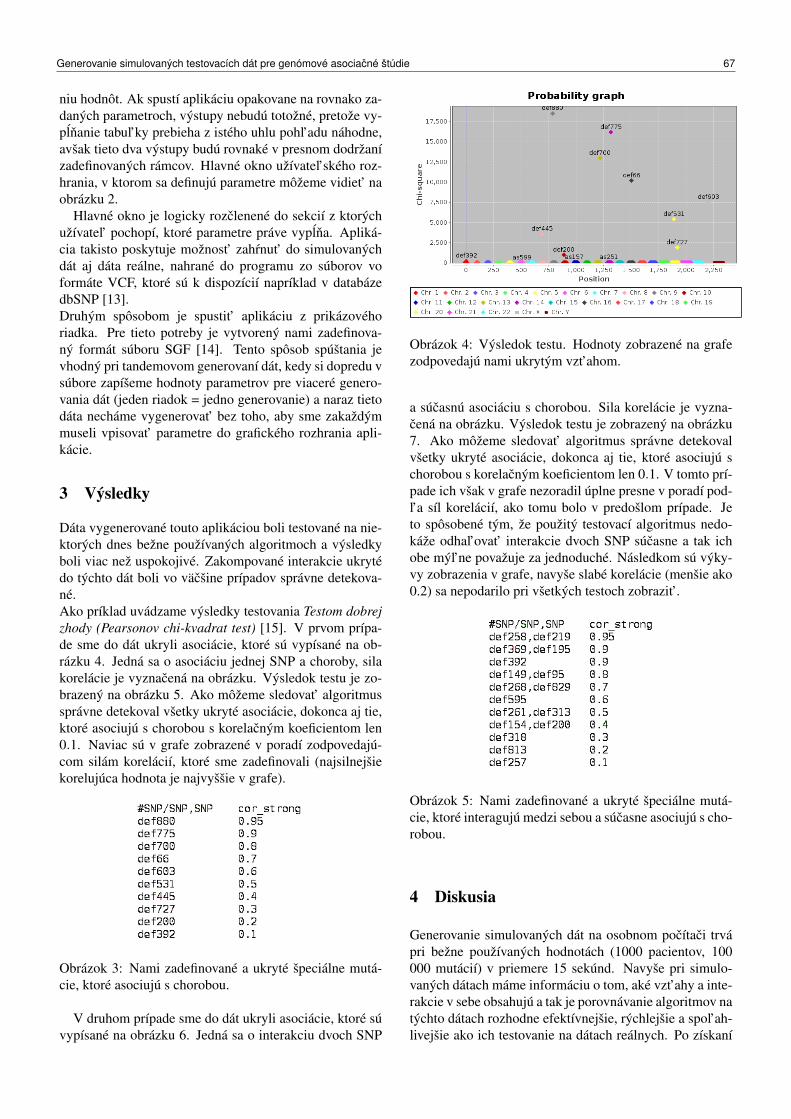
niu hodnôt. Ak spustí aplikáciu opakovane na rovnako za-daných parametroch, výstupy nebudú totožné, pretože vy-plnanie tabul’ky prebieha z istého uhlu pohl’adu náhodne,avšak tieto dva výstupy budú rovnaké v presnom dodržanízadefinovaných rámcov. Hlavné okno užívatel’ského roz-hrania, v ktorom sa definujú parametre môžeme vidiet’ naobrázku 2.

Hlavné okno je logicky rozclenené do sekcií z ktorýchužívatel’ pochopí, ktoré parametre práve vyplna. Apliká-cia takisto poskytuje možnost’ zahrnut’ do simulovanýchdát aj dáta reálne, nahrané do programu zo súborov voformáte VCF, ktoré sú k dispozícií napríklad v databázedbSNP [13].Druhým spôsobom je spustit’ aplikáciu z prikázovéhoriadka. Pre tieto potreby je vytvorený nami zadefinova-ný formát súboru SGF [14]. Tento spôsob spúštania jevhodný pri tandemovom generovaní dát, kedy si dopredu vsúbore zapíšeme hodnoty parametrov pre viaceré genero-vania dát (jeden riadok = jedno generovanie) a naraz tietodáta necháme vygenerovat’ bez toho, aby sme zakaždýmmuseli vpisovat’ parametre do grafického rozhrania apli-kácie.

3 Výsledky

Dáta vygenerované touto aplikáciou boli testované na nie-ktorých dnes bežne používaných algoritmoch a výsledkyboli viac než uspokojivé. Zakompované interakcie ukrytédo týchto dát boli vo väcšine prípadov správne detekova-né.Ako príklad uvádzame výsledky testovania Testom dobrejzhody (Pearsonov chi-kvadrat test) [15]. V prvom prípa-de sme do dát ukryli asociácie, ktoré sú vypísané na ob-rázku 4. Jedná sa o asociáciu jednej SNP a choroby, silakorelácie je vyznacená na obrázku. Výsledok testu je zo-brazený na obrázku 5. Ako môžeme sledovat’ algoritmussprávne detekoval všetky ukryté asociácie, dokonca aj tie,ktoré asociujú s chorobou s korelacným koeficientom len0.1. Naviac sú v grafe zobrazené v poradí zodpovedajú-com silám korelácií, ktoré sme zadefinovali (najsilnejšiekorelujúca hodnota je najvyššie v grafe).

Obrázok 3: Nami zadefinované a ukryté špeciálne mutá-cie, ktoré asociujú s chorobou.

V druhom prípade sme do dát ukryli asociácie, ktoré súvypísané na obrázku 6. Jedná sa o interakciu dvoch SNP

Obrázok 4: Výsledok testu. Hodnoty zobrazené na grafezodpovedajú nami ukrytým vzt’ahom.

a súcasnú asociáciu s chorobou. Sila korelácie je vyzna-cená na obrázku. Výsledok testu je zobrazený na obrázku7. Ako môžeme sledovat’ algoritmus správne detekovalvšetky ukryté asociácie, dokonca aj tie, ktoré asociujú schorobou s korelacným koeficientom len 0.1. V tomto prí-pade ich však v grafe nezoradil úplne presne v poradí pod-l’a síl korelácií, ako tomu bolo v predošlom prípade. Jeto spôsobené tým, že použitý testovací algoritmus nedo-káže odhal’ovat’ interakcie dvoch SNP súcasne a tak ichobe mýl’ne považuje za jednoduché. Následkom sú výky-vy zobrazenia v grafe, navyše slabé korelácie (menšie ako0.2) sa nepodarilo pri všetkých testoch zobrazit’.

Obrázok 5: Nami zadefinované a ukryté špeciálne mutá-cie, ktoré interagujú medzi sebou a súcasne asociujú s cho-robou.

4 Diskusia

Generovanie simulovaných dát na osobnom pocítaci trvápri bežne používaných hodnotách (1000 pacientov, 100000 mutácií) v priemere 15 sekúnd. Navyše pri simulo-vaných dátach máme informáciu o tom, aké vzt’ahy a inte-rakcie v sebe obsahujú a tak je porovnávanie algoritmov natýchto dátach rozhodne efektívnejšie, rýchlejšie a spol’ah-livejšie ako ich testovanie na dátach reálnych. Po získaní

Generovanie simulovaných testovacích dát pre genómové asociacné štúdie 67

Obrázok 6: Výsledok testu. Hodnoty zobrazené na grafezodpovedajú nami ukrytým vzt’ahom.

informácie o tom, že istý algoritmus preukázal spol’ahli-vost’ a korektnost’ na simulovaných dátach, je vyššia prav-depodobnost’, že po aplikovaní na reálne dáta bude tentoalgoritmus poskytovat’ správne výsledky a odhalí skrytéasociácie a interakcie v prírode. Navyše aplikácia nevyža-duje pre generovanie žiadnu formu reálných dát, avšak vprípade potreby poskytuje možnost’ zahrnut’ do simulova-ných dát bud’ dáta reálne alebo vygenerované inou apliká-ciou, co je vel’mi užitocným prvkom.V d’alšom výskume plánujeme aplikáciu rozšírit’ o LDbloky, kde bude jedna ci viacero SNP interagovat’ s ce-lým blokom. S tým súvisí aj vylepšenie závislosti SNP nachromozóme a pozícií na ktorej sa nachádza.

5 Thalamoss

Aplikácia bola primárne vytvorená pre potreby projek-tu THALAMOSS9. Tento projekt má za úlohu skúmat’a identifikovat’ SNP mutácie, ktoré zaprícinujú chorobu snázvom Talasémia - konkrétne β talasémiu [16]. Jedná sao dedicné ochorenie krvi, ktoré spôsobuje poruchy tvorbybielkovinových podjednotiek β . Tým je poškodené krv-né farbivo hemoglobín, co spôsobuje problémy s viazanímkyslíka v tele a jeho prenosom. Choroba má vel’mi t’ažkýpriebeh.

5.1 Pod’akovanie

Financná podpora bola poskytnutá projektom 7.RPEÚ "THALAssaemia MOdular Stratification Systemfor Personalized Therapy of Beta-Thalassaemia –THALAMOSS"(FP7-HEALTH-2012-INNOVATION-1(HEALTH.2012.1.2-1) Collaborative Project).

9http://thalamoss.eu/index.html

Referencie

[1] R.C. King, W.D. Stansfield, P.K. Mulligan: A dictionary ofgenetics, 7th ed., New York: Oxford University Press, 2006.

[2] N.J. Schork, D. Fallin, S. Lanchbury: Single nucleotide poly-morphisms and the future of genetic epidemiology. Clin Ge-net 58 (2000) 250–264

[3] The 1000 Genomes Project Consortium, A map of humangenome variation from population-scale sequencing. Nature467 (2010) 1061-1073

[4] The International HapMap Consortium, The InternationalHapMap Project. Nature 426 (2003) 789-796

[5] J. McEntyre, J. Ostell, editors: The NCBI Handbook. Bet-hesda (MD): National Center for Biotechnology Information(US), 2002

[6] W.S. Bush, J.H. Moore: Genome-Wide Association Studies.PLoS Comput Biol, Public Library of Science 8:12 (2012) s.e1002822

[7] P. Danecek, et.al.: The Variant Call Format and VCFtools,USA: Bioinformatics Advance Access, 2011

[8] P.C. Phillips: Epistasis — the essential role of gene interac-tions in the structure and evolution of genetic systems, Ore-gon: Center for Ecology and Evolution, University of Ore-gon, 2008.

[9] S. Purcell, B. Neale, K. Todd-Brown, L. Thomas, M.A.R.Ferreira, D. Bender, J. Maller, P. Sklar, P.I.W. de Bakker,M.J. Daly, P.C. Sham: PLINK: a toolset for whole-genomeassociation and population-based linkage analysis. Ameri-can Journal of Human Genetics, 2007

[10] F.A. Wright, et al.: Simulating association studies: a data-based resampling method for candidate regions or whole ge-nome scans. Bioinformatics 23 (2007) 2581-2588

[11] Ch. Li, M. Li: GWAsimulator: a rapid whole-genome si-mulation program. Bioinformatics 24 (2008) 140-142

[12] Z. Su, J. Marchini, P.Donnelly: HAPGEN2: simulation ofmultiple disease SNPs. Bioinformatics 27(16) (2011) 2304-2305

[13] S.T. Sherry, M. Ward, K. Sirotkin: dbSNP—Database forSingle Nucleotide Polymorphisms and Other Classes of Mi-nor Genetic Variation. Genome Research 9 (1999) 677–679

[14] S. Štefanic: Software na generování simulovaných testova-cích dat pro genomové asociacní studie (GWAS). Brno: Ma-sarykova univerzita, Fakulta informatiky, 2013

[15] D.C. Howell: CHI-SQUARE TEST - ANALYSIS OF CON-TINGENCY TABLES. Vermont: University of Vermont,2007

[16] R. Galanello, R. Origa: Beta-thalassemia. Orphanet Jour-nal of Rare Diseases 5 (2010)

68 S. Štefanic, M. Lexa

Comparative Genomics in Genome Projects(Abstract)

Tomáš Vinar, Brona Brejová

Faculty of Mathematics, Physics, and Informatics, Comenius University in Bratislava, Mlynská dolina, 842 48 Bratislava, Slovakiavinar,brejova@fmph.uniba.sk

We will describe contributions of our research group tolarge international genome projects. These contributionscan be divided into two categories: genome annotation andpositive selection analysis.

Genome annotation. In recent years, major lowering ofgenome sequencing costs brought large availability ofnovel genome sequences. Annotation of protein codinggenes is one of the basic steps in their analysis. A tradi-tional way of annotating genes is to first create a manu-ally curated set of high-confidence gene models, use it totrain parameters a gene finding program, and then use thisprogram to predict genes on the whole-genome scale. Re-training is required for each newly sequenced organism,unless gene finder paramters are available for a closely re-lated species.

Unfortunately, creating these training sets is a difficultand time consuming process, limiting our ability to obtainreliable annotations for newly sequenced genomes. To ad-dress this problem, we use a variety of information, in-cluding known protein sequences (from other genomes),similarity to related genomes, and experimental evidenceof transcription (RNASeq) to train a gene finder in an au-tomated way [1]. We are using these tools in genomeprojects to provide an initial protein coding gene annota-tion that is used as a basis of further analysis [9, 10].

Positive selection analysis. Detection of positive selec-tion is a key step in identification of genes responsible forspecific phenotypic traits of a particular organism. In ourearlier work [3], we have summarized an analysis frame-work based on codon-substitution models of Yang andNielsen [8], and applied it to then available mammaliangenomes. We have applied our methodology in the contextof several vertebrate genome projects [2, 4, 5, 6]. Amongother results, we have demonstrated that several func-tional categories (e.g. immunity, defense) are consistentlyenriched for positively selected genes, while other cate-gories (e.g., genes related to basic cellular processes) arestrongly conserved throughout vertebrate evolution. Wehave discovered several gene mutations likely responsiblefor lineage-specific traits and characterized differences be-tween evolution of protein coding genes in mammals androdents. We have demonstrated that duplicated gene clus-ters are generally enriched for positive selection and pro-vided tools for analysis of genome regions accumulatingsegmental duplications [2, 7, 5]. We have also provided

comprehensive lists of genes positively selected on indi-vidual lineages and clades that can be studied in more de-tail by specialists.

Outlook. With the cost of sequencing of a human-sizedgenome soon to be lower than the open access fee for asingle publication, it is clear that sequencing efforts willcontinue to boom in the near future. A major effort of se-quencing 10,000 vertebrate genomes currently under waywill create a huge opportunity for comparative genomics.However, tools currently available are designed for com-parative analysis of tens of genomes at best. Thus, there isa clear need for designing new methods that will scale tothousands of genome instead.

References

[1] B. Brejova, T. Vinar, Y. Chen, S. Wang, G. Zhao, D. G.Brown, M. Li, and Y. Zhou. Finding genes in Schistosomajaponicum: annotating novel genomes with help of extrin-sic evidence. Nucleic Acids Res, 37(7):e52, 2009.

[2] R. A. Gibbs et al. Evolutionary and biomedical in-sights from the rhesus macaque genome. Science,316(5822):222–224, 2007.

[3] C. Kosiol, T. Vinar, R. R. da Fonseca, M. J. Hubisz, C. D.Bustamante, R. Nielsen, and A. Siepel. Patterns of pos-itive selection in six Mammalian genomes. PLoS Genet,4(8):e1000144, 2008.

[4] R. Li et al. The sequence and de novo assembly of the giantpanda genome. Nature, 463(7279):311–317, 2010.

[5] D. P. Locke et al. Comparative and demographic analysisof orang-utan genomes. Nature, 469(7331):529–533, 2011.

[6] B. H. Shaffer et al. The western painted turtle genome,a model for the evolution of extreme physiological adap-tations in a slowly evolving lineage. Genome Biol,14(3):R28, 2013.

[7] T. Vinar, B. Brejova, G. Song, and A. Siepel. Reconstruct-ing histories of complex gene clusters on a phylogeny. JComput Biol, 17(9):1267–1269, 2010.

[8] Z. Yang and R. Nielsen. Codon-substitution models for de-tecting molecular adaptation at individual sites along spe-cific lineages. Mol Biol Evol, 19(6):908–917, 2002.

[9] Y. Zhou et al. The Schistosoma japonicum genome revealsfeatures of host-parasite interplay. Nature, 460(7253):345–351, 2009.

[10] S. Zhu et al. Sequencing the genome of Marssonina brun-nea reveals fungus-poplar co-evolution. BMC Genomics,13:382, 2012.

ITAT 2013: Workshops, Posters, and Tutorials, p. 69ISBN 978-1490952086, c© 2013 T. Vinar, B. Brejová

Workshop on Computational Intelligenceand Data Mining

The workshop “Computational Intelligence and Data Mining” has been organized as a part of theconference ITAT 2013. The workshop is mainly targeted at participants with research interests inevolutionary computing, artificial neural networks, and fuzzy logic. The participants were invitedto submit a paper in English of up to eight pages, prepared according to the instructions at ITAT2013 web pages. The authors of the best papers from the workshop will be invited to submitan extended version of their work to the journal Neural Network World, published by the CzechTechnical University and covered in Science Citation Index Expanded and Current Contents.

A key factor influencing the overall quality of the workshop and of the final versions of thesubmitted papers published in these proceedings was the program committee. “ComputationalIntelligence and Data Mining” is grateful to 22 reviewers who read the submitted papers, andhave provided competent, and in most cases very detailed, feedback to their authors. Nearlyall program committee members regularly review papers for first-class international journals, andmany of them are leading Czech scientists in their particular areas of computational intelligence,with an international reputation witnessed by hundreds of citations.

Each submitted paper was anonymously reviewed by at least three of the program committeemembers. The papers were evaluated according to a seven-grade scale from “strong reject”to “strong accept”. In the end, the workshop program committee only accepted papers, whereno referee suggested (even weak) rejection and the mean score of the paper was positive. Thisvolume presents final versions of seven papers that were accepted for the workshop presentation.

Martin HolenaAcademy of Sciences of the Czech RepublicWorkshop Program Chair

71

Workshop Program Committee

Petr Berka, University of Economics, Faculty of Informatics and StatisticsJan Faigl, Czech Technical University, Faculty of Electrical EngineeringFrantišek Hakl, Academy of Sciences of the Czech Republic, Institute of Computer ScienceDavid Hartman, Charles University, Facutly of Mathematics and PhysicsJaroslav Hlinka, Academy of Sciences of the Czech Republic, Institute of ComputerScienceMartin Holena, Academy of Sciences of the Czech Republic, Institute of Computer ScienceJán Hric, Charles University, Facutly of Mathematics and PhysicsMarcel Jirina, Academy of Sciences of the Czech Republic, Institute of Computer ScienceJan Kalina, Academy of Sciences of the Czech Republic, Institute of Computer ScienceTomáš Kliegr, University of Economics, Faculty of Informatics and StatisticsJirí Kléma, Czech Technical University, Faculty of Electrical EngineeringPavel Kordík, Czech Technical University, Faculty of Information TechnologyJirí Kubalík, Czech Technical University, Faculty of Electrical EngineeringJaromír Kukal, Czech Technical University, Faculty of Nuclear Sciences and Physical EngineeringMirko Navara, Czech Technical University, Faculty of Electrical EngineeringRoman Neruda, Academy of Sciences of the Czech Republic, Institute of Computer ScienceTomáš Pevný, Czech Technical University, Faculty of Electrical EngineeringPetr Pošík, Czech Technical University, Faculty of Electrical EngineeringJan Rauch, University of Economics, Faculty of Informatics and StatisticsMiroslav Šnorek, Czech Technical University, Faculty of Electrical EngineeringMartin Vejmelka, Academy of Sciences of the Czech Republic, Institute of Computer ScienceMarta Vomlelová, Charles University, Facutly of Mathematics and Physics

Representations of highly-varying functions by perceptron networks

Vera Kurková

Institute of Computer Science, Academy of Sciences of the Czech,vera@cs.cas.cz,

WWW home page: http://www.cs.cas.cz/ vera

Abstract: Tractability of representations of multivari-able functions by perceptron networks is investigated.There are described classes of functions which cannot betractably represented by Heaviside perceptron networks inthe sense that all their representations by such networks re-quire numbers of units or sizes of output weights depend-ing exponentially on the number of variables d. It is shownthat the concept of variational norm from approximationtheory can play a role of a measure of such tractability. Ex-istence of large sets of Boolean functions with variationsdepending on d exponentially is proven. The results areillustrated by an example of a class of Boolean functionsdefined in terms of their communication matrices.

1 Introduction

A widely-used type of a neural-network architecture is theone-hidden-layer network. Typical computational units inthe hidden layer are perceptrons, radial, and kernel units.A variety of learning algorithms have been developed andsuccessfully applied to adjust parameters of such networks(see, e.g., [8, 7] and the references therein). Recently, one-hidden-layer networks have been called shallow networksto distinguish them from deep ones, which contain morehidden layers.

Shallow networks with many types of computationalunits are known to be universal approximators, i.e., theycan approximate up to any desired accuracy all contin-uous functions or L p-functions on compact subsets ofRd . In particular, the universal approximation propertyholds for one-hidden-layer networks with perceptrons hav-ing any non-polynomial activation function [17, 23] andwith radial and kernel units satisfying mild conditions[22, 20, 14], [26, p.153]. Moreover, all functions definedon finite subsets of Rd can be exactly represented by one-hidden-layer networks with sigmoidal perceptrons [10] orwith Gaussian kernel units [21].

Proofs of the universal approximation capability of one-hidden-layer networks require potentially unlimited num-bers of hidden units. These numbers representing modelcomplexities of the networks are critical factors for prac-tical implementations. Dependence of model complexi-ties of shallow networks on their input dimensions, typesof units, functions to be approximated, and accuracies ofapproximation have been studied using tools from nonlin-ear approximation theory. Some estimates were derivedfrom upper bounds on rates of approximation of various

classes of multivariable functions by networks with in-creasing numbers of hidden units (see, e.g., [11] and ref-erences therein). On the other hand, limitations of compu-tational capabilities of one-hidden-layer networks are lessunderstood. Only few lower bounds on rates of approxi-mations by such networks are known. Moreover the lowerbounds are mostly non constructive and hold for types ofcomputational units that are not commonly used [18, 19].Also growth of sizes of weights is not well understood, itwas shown that in some cases, reasonable sizes of weightsare more important for successful learning than bounds onnumbers of network units [4].

Recently new learning algorithms, which can be ap-plied to deep networks, were developed (see, e.g., [5, 9]).As training networks with more than one hidden layerinvolves complicated nonlinear optimization procedures,generally it is more difficult than training shallow ones.Hence, it is desirable to develop some theoretical back-ground for characterization of tasks whose computingby shallow networks requires models with considerablylarger numbers of units and/or sizes of weights than com-puting by deep ones. Since typical neurocomputing appli-cations deal with large numbers of variables, it is partic-ularly important to understand how quickly model com-plexities of shallow networks grow with increasing inputdimensions.

To contribute to such understanding, in this paper weinvestigate classes of multivariable functions whose rep-resentations by shallow networks are not tractable in thesense that the numbers of network hidden units or sizesof their output weights grow exponentially with increas-ing input dimensions. We propose to use the concept ofvariational norm from approximation theory as a measureof “amount of variations of a function”, which was sug-gested by Bengio et al. [6] as a cause of difficulties inrepresenting functions by shallow networks. We show thatthe size of the variational norm with respect to a dictionaryof computational units reflects both the number of hiddenunits and sizes of output weights. We derive lower boundson probabilistic measures of sets of real-valued Booleanfunctions having “large” variations. For Heaviside percep-tron networks, we prove that a probability that a functionsof a given Euclidean norm has a “large” variation (depend-ing on d exponentially) grows with d exponentially, i.e.,that for large dimensions in sets of functions with con-stant Euclidean norms most Boolean real-valued functionscannot be tractably represented by Heaviside perceptron

ITAT 2013: Workshops, Posters, and Tutorials, pp. 73–76ISBN 978-1490952086, c© 2013 V. Kurková

networks. We describe a concrete class of non tractablefunctions in terms of properties of their communicationmatrices.

The paper is organized as follows. Section 2 con-tains basic concepts on shallow perceptron networks andBoolean functions. Section 3 proposes a mathematical for-malization of the concept of a “highly-varying function”,shows that it is related to large model complexities or sizesof weights in networks representing such functions, andgives estimates of probabilistic measures of sets of func-tions with variations depending on d exponentially. Sec-tion 4 illustrates general results by examples of Booleanfunctions with Hadamard communication matrices.

2 Preliminaries

One-hidden-layer networks with single linear outputs (re-cently called shallow networks) compute input-outputfunctions from sets of the form

spann G :=

n

∑i=1

wigi |wi ∈ R, gi ∈ G

,

where G, called a dictionary, is a set of functions com-putable by a given type of units, the coefficients wi arecalled output weights, and n is the number of hidden units.This number is sometimes used as a measure of modelcomplexity. In this paper we use the terminology “one-hidden-layer network” meaning a network with a singlelinear output.

We investigate growth of network complexities repre-senting functions of increasing numbers of variables d.Let D be an infinite subset of the set of positive integers,F = fd |d ∈ D a class of functions and Gd |d ∈ Da class of dictionaries, such that for every d ∈ D, fd is afunction of d variables and Gd is formed by functions ofd variables. We call the problem of representing the setF by networks from spanGd |d ∈D tractable if for ev-ery d ∈ D, there exists a network in spannd

G representingfd as its input-output function such that nd and absolutevalues of all output weights in the network grow with dpolynomially. Note that different concepts of tractabilitywere used in other contexts (see, e.g., [11]).

In this paper, we focus on representations of real-valuedBoolean functions by one-hidden-layer perceptron net-works. By

B(0,1d) := f | f : 0,1d → R

we denote the space of real-valued Boolean functions of d-variables. This space is isomorphic to the Euclidean spaceR2d

and thus on B(0,1d) we have the Euclidean innerproduct defined as

〈 f ,g〉 := ∑u∈0,1d

f (u)g(u)

and the Euclidean norm ‖ f‖2 :=√〈 f , f 〉. By · we denote

the inner product on 0,1d , defined as u · v := ∑di=1 uivi.

We consider two dictionaries of computational units,which are subsets of B(0,1d). The first one is the setHd of functions on 0,1d computable by Heaviside per-ceptrons, i.e.,

Hd := ϑ(v · .+b) : 0,1d →0,1|v ∈ Rd ,b ∈ R ,where ϑ denotes the Heaviside activation function definedas ϑ(t) := 0 for t < 0 and ϑ(t) := 1for t ≥ 0. Note thatHd is the set of characteristic functions of half-spaces. Thesecond dictionary Pd is closely related to Hd . It is formedby functions from B(0,1d) computable by perceptronswith signum activation function sgn :R→−1,1 definedas sgn(t) := −1 for t < 0 and sign(t) := 1 for t ≥ 0. Wedenote

Pd := sgn(v · .+b) : 0,1d →−1,1|v ∈ Rd ,b ∈ R .

3 Highly-varying functions

In this section, we use the concept of a variational normfrom approximation theory as a measure of tractability ofa representation of a class of function by one-hidden-layernetwork.

For a subset G of a normed linear space (X ,‖.‖X ), G-variation (variation with respect to the set G), denoted by‖.‖G, is defined as

‖ f‖G := infc ∈ R+ | f/c ∈ clX conv(G∪−G) ,where clX denotes the closure with respect to the norm‖ · ‖X on X , −G := −g | g ∈ G, and convG :=

∑ki=1 aigi | ai ∈ [0,1],∑k

i=1 ai = 1,gi ∈ G,k ∈ N

is theconvex hull of G.

Variation with respect to a set of functions was intro-duced by Kurková [13] as an extension of Barron’s [2]concept of variation with respect to sets of characteris-tic functions. Barron focused on the set of characteristicfunctions of half-spaces, which corresponds to the dictio-nary of functions computable by Heaviside perceptrons.For d = 1, variation with respect to half-spaces coincidesup to a constant with the concept of total variation from in-tegration theory. Variational norms play an important rolein estimates of approximation rates by one-hidden-layernetworks (see, e.g., [3, 15, 11] and the references therein).

The following straightforward consequence of the defi-nition of G-variation shows that in all representations of afunction with “large” G-variation by networks with unitsfrom G, the number of units must be “large” or some ab-solute values of output weights must be “large”.

Proposition 1. Let G be a bounded subset of a normedlinear space (X ,‖.‖), then for every f ∈X , ‖ f‖G ≤min

∑k

i=1 |wi|∣∣∣ f = ∑k

i=1 wi gi , wi ∈ R, gi ∈ G,k ∈ N

and for G finite with cardG = k,‖ f‖G = min

∑k

i=1 |wi|∣∣∣ f = ∑k

i=1 wi gi , wi ∈ R, gi ∈ G.

74 V. Kurková

Proof. The first statement follows directly from the defi-nition and the second one holds as for G finite, convG isclosed.

Thus families of sets of d-variable functions Fd |d ∈Dwith Gd-variations growing with d exponentially cannotbe tractably represented by networks with units from Gd .To describe such classes of functions, we use the followinglower bound on variational norm from [16].

Theorem 2. Let (X ,‖.‖X ) be a Hilbert space and G itsbounded subset. Then for every f ∈X \G⊥,

‖ f‖G ≥ ‖ f‖2supg∈G |g· f | .

Theorem 2 implies that functions which are “almost or-thogonal” to G have large variations. Note that G-variationis a norm and thus by multiplying f by suitable constantswe can obtain functions with arbitrarily large or small vari-ations. However in neurocomputing, we are usually in-terested in computation of functions with similar sizes ascomputational units. Also in theory of circuit complexity,representations of classes of functions of fixed Euclideannorms by networks with gates computing functions withthe same norms are investigated (see, e.g., [24]). In partic-ular, representations of Boolean functions with values in−1,1 by networks composed from signum perceptronsare studied. All these functions have Euclidean normsequal to 2d/2.

The maximum of the l2-norms of the elements of thedictionary Hd formed by functions from B(0,1d) com-putable by Heaviside perceptrons is 2d/2 and the norms ofall elements of Pd are equal to 2d/2. Thus it is reasonableto explore distributions of variations of functions in thespheres S2d−1

2d/2 of radii 2d/2 in B(0,1d).Consider an angular pseudometrics δ defined on the

unit ball S2d−1 in R2das

δ ( f ,g) = arccos | f ·g|.

This pseudometrics defines the distance as the minimumof the two angles between f and g and between f and −g(it is a pseudometrics as the distance of antipodal vectorsis zero).

The following theorem estimates probability that a ran-domly chosen Boolean function of d variables with the Eu-clidean norm 2d/2 has variation with respect to Heavisideperceptrons larger than 1

cos α .

Theorem 3. Let d be a positive integer, µ a uniformmeasure on S2d−1

2d/2 such that µ(S2d−12d/2 ) = 1, α ∈ (0,π/2),

and Vα = f ∈ S2d−12d/2 |‖ f‖Hd ≥ ‖ f‖Pd ≥ 1

cos α . Then

µ(Vα)≥ 1−2d2e−

(2d−1)(cos α)22 .

Proof. By Theorem 2, Vα contains all f ∈ S2d−12d/2 satisfy-

ing for all g ∈ Pd , | f ·g| ≤ cosα , i.e., all f with δ ( f ,g) =arccos | f ·g| ≥α . This means that f is not contained in anyof the spherical caps C(g,ε) with a center g∈ Pd and angle

α = arccos ε defined as C(g,ε) = h ∈ S2d−12d/2 |h · g ≥ ε.

With d increasing, the normalized measures of the spher-ical caps are decreasing exponentially fast: µ(C(g,ε)) ≤e−mε2/2 (see, e.g., [1, p.11]). Schläfli [25] derived an upperbound 2d2−d log2 d+O(d) on the number of subsets of 0,1d

obtained by intersecting 0,1d with half-spaces. Thuscardinalities of both dictionaries Hd and Pd are smaller

than 2d2. Hence µ(Vα)≥ 1−2d2

e−2d (cos α)2

2 .

Setting cos α = (2d −1)−1/4, we obtain from Theorem

3 the lower bound 1−e−(2d−1)1/2−2d2

2 on the relative size ofthe subset of the ball of radius 2d/2 in B(0,1d) contain-ing functions with variations with respect to half-spaceslarger or equal to (2d −1)1/4. So by Proposition 1, a ran-domly chosen real-valued Boolean function of the norm2d/2 cannot be tractably represented by a shallow Heavi-side perceptron network.

4 Examples

In the previous section, we proved that there exist “large”sets of functions with exponentially large variations. Someconcrete examples of such functions can be obtained us-ing representations of Boolean functions as communica-tion matrices. Recall that the communication matrix of afunction f : 0,1d→−1,1 with d even is a 2d/2×2d/2

matrix M( f ) with rows and columns indexed by vectorsu,v ∈ 0,1d/2 such that

M( f )u,v := f (u∗ v),

where ∗ denotes the concatenation of two vectors in0,1d/2 defined for u,v ∈ 0,1d/2 as (u ∗ v)i := ui fori = 1, . . . ,d/2 and (u∗ v)i := vi for i = d/2+1, . . . ,d.

Recall that a square matrix with entries in −1,1 iscalled Hadamard if each pair of its rows (columns, resp.)is orthogonal. The following theorem obtained as a re-formulation of [16, Theorem 3.7] gives a lower bound onHd-variations of functions with Hadamard communicationmatrices. The notation h = Ω(g(d)) with two functionsg,h : N→ R means that there exist a positive constant cand n0 ∈ N such that for all n ≥ no one has h(n) ≥ cg(n)[12].

Theorem 4. Let d be an even integer, f : 0,1d →−1,1 a function with a Hadamard communication ma-trix, and f (x) = ∑m

i=1 wiϑ(vi · x+bi) its representation bya one-hidden-layer Heaviside perceptron network. Then∑m

i=1 |wi|= Ω(22d/6) .

Proof. It was shown in [16, Theorem 3.7] that under theassumptions of the theorem, ‖ f‖Pd = Ω(2d/6). By [15,Proposition 3], for every h ∈ Hd , ‖h‖Pd ≤ 1. So ‖.‖Pd ≤‖.‖Hd . The statement then follows from Proposition 1.

Theorem 4 implies that a representation of a class of d-variable Boolean functions with Hadamard communica-tion matrices by one-hidden-layer Heaviside perceptron

Representations of Highly-Varying Functions by Perceptron Networks 75

networks is not tractable. These functions cannot be repre-sented by Heaviside perceptron networks with polynomi-ally bounded numbers of units and sums of absolute valuesof output weights.

A paradigmatic example of a class of functions withHadamard comunication matrices are functions βd :0,1d → −1,1 defined for every even positive integerd and all x ∈ 0,1d as

βd := (−1)l(x)·r(x)

where l(x),r(x) ∈ 0,1d/2 are defined for every i =1, . . . ,d/2 as l(x)i := xi and r(x)i := xd/2+i. When therange −1,1 is replaced with 1,0, these functionscompute inner product of l(x) with r(x) mod 2, and thusthey are called ‘inner product mod 2”. It is well-knownand easy to check that for every even integer d, the com-munication matrix M(βd) is Hadamard (see, e.g., [24]).

The functions “inner prod mod 2” were used in theoryof circuit complexity as an example of a class of func-tions which cannot be expressed as depth-2 polynomialsize circuits with weights being polynomially bounded in-tegers [24]. Our results are stronger as they include alsoother functions with Hadamard communication matricesand also hold for weights which are real numbers.

Acknowledgments. This work was partially supported byGA CR grant P202/11/1368 and an institutional support ofthe Institute of Computer Science RVO 67985807.

References

[1] K. Ball. An elementary introduction to modern convex ge-ometry. In S. Levy, editor, Falvors of Geometry, pages 1–58. Cambridge University Press, 1997.

[2] A. R. Barron. Neural net approximation. In K. Narendra,editor, Proc. 7th Yale Workshop on Adaptive and LearningSystems, pages 69–72. Yale University Press, 1992.

[3] A. R. Barron. Universal approximation bounds for superpo-sitions of a sigmoidal function. IEEE Trans. on InformationTheory, 39:930–945, 1993.

[4] P. L. Bartlett. The sample complexity of pattern classifica-tion with neural networks: The size of the weights is moreimportant than the size of the network. IEEE Trans. on In-formation Theory, 44:525–536, 1998.

[5] Y. Bengio. Learning deep architectures for AI. Foundationsand Trends in Machine Learning, 2:1–127, 2009.

[6] Y. Bengio, O. Delalleau, and N. Le Roux. The curse ofhighly variable functions for local kernel machines. In Ad-vances in Neural Information Processing Systems 18, pages107–114. MIT Press, 2006.

[7] T. W. S. Chow and S. Y. Cho. Neural Networks and Com-puting: Learning Algorithms and Applications. World Sci-entific, 2007.

[8] T. L. Fine. Feedforward Neural Network Methodology.Springer, Berlin Heidelberg, 1999.

[9] G. E. Hinton, S. Osindero, and Y. W. Teh. A fast learn-ing algorithm for deep belief nets. Neural Computation,18:1527–1554, 2006.

[10] Y. Ito. Finite mapping by neural networks and truth func-tions. Mathematical Scientist, 17:69–77, 1992.

[11] P. C. Kainen, V. Kurková, and M. Sanguineti. Dependenceof computational models on input dimension: Tractabilityof approximation and optimization tasks. IEEE Trans. onInformation Theory, 58:1203–1214, 2012.

[12] D. E. Knuth. Big omicron and big omega and big theta.SIGACT News, 8:18–24, 1976.

[13] V. Kurková. Dimension-independent rates of approxima-tion by neural networks. In K. Warwick and M. Kárný, ed-itors, Computer-Intensive Methods in Control and SignalProcessing. The Curse of Dimensionality, pages 261–270.Birkhäuser, Boston, MA, 1997.

[14] V. Kurková. Some comparisons of networks with radial andkernel units. In A.E.P. Villa, W. Duch, P. Érdi, F. Masulli,and G. Palm, editors, Neural Networks: Brain-inspiredComputing and Machine Learning Research, volume 7553of Lecture Notes in Computer Science, pages II. 17–24.Springer-Verlag, Berlin, Heidelberg, 2012.

[15] V. Kurková and M. Sanguineti. Comparison of worst-caseerrors in linear and neural network approximation. IEEETrans. on Information Theory, 48:264–275, 2002.

[16] V. Kurková, P. Savický, and K. Hlavácková. Representa-tions and rates of approximation of real–valued Booleanfunctions by neural networks. Neural Networks, 11:651–659, 1998.

[17] M. Leshno, V. Ya. Lin, A. Pinkus, and S. Schocken. Mul-tilayer feedforward networks with a nonpolynomial activa-tion function can approximate any function. Neural Net-works, 6:861–867, 1993.

[18] V. Maiorov. On best approximation by ridge functions. J.of Approximation Theory, 99:68–94, 1999.

[19] V. Maiorov and A. Pinkus. Lower bounds for approxima-tion by MLP neural networks. Neurocomputing, 25:81–91,1999.

[20] H. N. Mhaskar. Versatile Gaussian networks. In Proceed-ings of IEEE Workshop of Nonlinear Image Processing,pages 70–73, 1995.

[21] C. A. Micchelli. Interpolation of scattered data: Distancematrices and conditionally positive definite functions. Con-structive Approximation, 2:11–22, 1986.

[22] J. Park and I. Sandberg. Approximation and radial-basis-function networks. Neural Computation, 5:305–316, 1993.

[23] A. Pinkus. Approximation theory of the MLP model inneural networks. Acta Numerica, 8:143–195, 1999.

[24] V. Roychowdury, K. Siu, and A. Orlitsky. Neural modelsand spectralmethods. In Theoretical Advances in NeuralComputation and Learning, pages 3–36. Kluwer AcademicPublishers, Dodrecht, 1994.

[25] L. Schläfli. Theorie der vielfachen Kontinuität. Zürcher &Furrer, Zürich, 1901.

[26] I. Steinwart and A. Christmann. Support Vector Machines.Springer, new York, 2008.

76 V. Kurková

Application of Copulas to Data MiningBased on Observational Logic

Martin Holena1 and Martin Scavnicky2

1 Institute of Computer Science, Academy of Sciences of the Czech RepublicPod vodarenskou vezı 2, 18207 Prague

2 Faculty of Mathematics and Physics, Charles UniversityMalostranske namestı 25, 118 00 Prague

Abstract. The objective of the paper is a small contribu-tion to data mining based on observational logic – introduc-ing generalized quantifiers inspired by copulas. Fitting co-pulas to multidimensional data is an increasingly importantmethod for analyzing dependencies, and the new quantifiersof observational logic assess the possibility to describe thedata by a hierarchical Archimedean copula with given prop-erties. To this end, basic concepts pertaining to copulas,Archimedean copulas and hierarchical Archimedean copu-las are first recalled, together with those properties that willbe needed for the definition of the new quantifiers. Since theresult of assessing the possibility to describe the data by acopula depends not only on the properties of that copula,but also on the precise algorithm for fitting it to the data,we present the algorithm we have used to this end, beforefinally defining the new quantifiers. The paper concludeswith a brief illustration of applying the proposed quanti-fiers to the well-known Iris data set.

1 Introduction

One of the main directions in data mining is extract-ing various kinds of logical rules, such as classificationrules, association rules or fuzzy rules from the avail-able data [1, 6, 12, 20, 29, 32]. Logical rules, especiallythe Boolean IF . . . THEN rules (Boolean implications)are considered easily understandable for humans andclose to the human way of thinking. However, the se-mantics of Boolean logic is not rich enough to conveythe diversified knowledge obtained through data min-ing. A very early generalization of the classical (i.e.,Boolean) predicate calculus in that direction is the ob-servational logic, elaborated in the 1970s [9]. It extendsthe classical predicate calculus with generalized quan-tifiers, assessing the results of operations with datasamples. In this way, it provides a semantics that isrich enough to convey the knowledge obtained throughanalyzing the data.

In the first two decades after observational logicoriginated, only binary generalized quantifiers basedon the estimation of particular probabilities and onseveral simple hypothesis tests were considered, both

in theory and in the implementation of a particularrules-extraction method based on observational logic,known under the acronym GUHA (General Unary Hy-potheses Automaton) [8, 9]. This was due to the veryimportant role that those two kinds of statistical meth-ods play, as well as due to the comparatively low com-putational costs of evaluating formulas with such gen-eralized quantifiers. For the latter reason, only quan-tifiers for binary or dichotomized data were used atthat time. Moreover, all of them are based only on esti-mates and tests constructed by means of the 2×2-foldcontingency table of the two considered variables. Dur-ing the last 10-15 years, on the other hand, quantifiersbased on other data analysis methods have been in-troduced, in particular, on general contingency tables,on estimates of joint distributions of multivariate dis-crete variables, on trend changes in time series, and onfuzzy hypotheses testing [15, 16, 26–28]. A survey canbe found in [11], whereas much of the underlying the-oretical developments of observational logic has beenpresented in the recent monograph [29].

The present paper follows this line of research. Itproposes generalized quantifiers related to an increas-ingly important method of analyzing dependencies inmultidimensional data – estimating the structure ofjoint distributions of continuous variables by meansof copulas, especially by means of hierarchical Archi-medean copulas. The concept of copulas as a meansallowing to describe the relationship between a jointdistribution and its marginals has been introduced asearly as in the late 1950s [30]. However, their increas-ing use in data analysis is a matter of only the last10-15 years [3, 17, 22], when the commonly availablecomputing power has made it affordable to fit copulaseven to medium-sized data.

In the next section, fundamentals of observationallogic are recalled. Section 3 summarizes definitions andproperties pertaining to hierarchical Archimedean co-pulas. In Section 4, which is the key section of thepaper, three new observational quantifiers are intro-duced assessing the possibility to describe given databy a hierarchical Archimedean copula with given prop-erties. Because of the limited extent of the paper, the

ITAT 2013: Workshops, Posters, and Tutorials, pp. 77–85ISBN 978-1490952086, c© 2013 M. Holena, M. Šcavnický

new quantifiers are illustrated only on one data set,the well-known Iris data benchmark.

2 Observational Logic for DataMining

Observational logic is an extension of classical monadicpredicate calculus that has only unary predicates. Inparticular:(i) Its language is a superset of the language of Boo-

lean logic with unary predicates, extending thatlanguage with symbols for generalized quantifiers,which will be introduced below. Apart of thoseadditional symbols, it has all the symbols of theoriginal language, i.e., symbols for the unary pred-icates and their single variable (which can be leftout due to its uniqueness), various logical connec-tives (¬,&,∨, . . . ), logical constants 1 and 0, andthe quantifiers ∀ (universal) and ∃ (existential).

(ii) Formulas of the language containing neither any∀ nor any ∃ are called open formulas, e.g.disease duration > 10 years & sex = male

& ¬epileptic fits.(iii) If the unary predicates have been evaluated as

true (1) or false (0) on some data (e.g., in the ex-ample above, if the predicates disease duration

> 10 years, sex = male and epileptic fits

have been evaluated based on the data of somepatient), then any open formula can be evaluatedusing standard rules for the evaluation of Booleanconnectives and the quantifiers ∀ and ∃The theory of observational logic has been rigor-

ously elaborated in [9]. Here, only the definitions ofa generalized quantifier and of its evaluation will berecalled.

Definition 1. Consider a language of Boolean logicwith unary predicates, and let Q be a symbol not be-longing to the symbols of that language. Let furtherm ∈ N , ϕ1, . . . , ϕm be open formulas of the language,and TfQ be a 0/1-valued function on Boolean matriceswith m columns, i.e.,

TfQ :⋃

n∈N0, 1n,m → 0, 1. (1)

Then:

a) Q is called generalized quantifier of arity m, andit belongs to symbols of the language of observa-tional logic that includes the considered languageof Boolean logic, TfQ is called truth function ofQ.

b) The formula Q(ϕ1, . . . , ϕm) is a formula of theconsidered language of observational logic. How-ever, that formula is not called open formula, butclosed formula.

In the case of a binary generalized quantifier ∼, thesimplified notation ϕ1 ∼ ϕ2 instead of ∼ (ϕ1, ϕ2) isused.

Definition 2. Let m ∈ N , ϕ1, . . . , ϕm be open formu-las, and Q be an m-ary generalized quantifier with atruth function TfQ. Let further D ∈ <n,m be a datamatrix with rows d1, . . . , dn, and for i = 1, . . . , n, j =1, . . . ,m, let ‖ϕj‖i be the evaluation of ϕj based ondi according to (iii) above. Then the evaluation ofQ(ϕ1, . . . , ϕm) based on D is the value

TfQ

‖ϕ1‖1 . . . ‖ϕm‖1. . . . . . . . . . . . . . . . . . . . . . . . .

‖ϕ1‖n . . . ‖ϕm‖n.

(2)

Observe that the truth function (1) of a quanti-fier can be defined quite generally. Nevertheless, forall quantifiers really used in data mining, it has al-ways been defined so as to assess the results of someoperations with the data. In the early decades afterobservational logic originated, those operations werealways either the estimation of particular probabili-ties, or simple hypotheses tests.

Example 1. The quantifier founded implication →θ

with a threshold θ ∈ (0, 1) corresponds to estimat-ing the conditional probability PC|A of the validityof the consequent on condition of the validity of theantecedent. It underlies the restriction that the esti-mation is performed only if the simultaneous validityof antecedent and consequent in the data achieves atleast a prescribed basic level B ∈ N . Apart from thisrestriction, the constructed estimate is unbiased andconsistent. Its truth function is defined

(∀n ∈ N )(∀x = (x(i)1 , x

(i)2 )i=1,...,n ∈ 0, 1n,2)

Tf→θ(x) =

1 if∑ni=1 x

(i)1 x

(i)2 ≥ B &Pn

i=1 x(i)1 x

(i)2Pn

i=1 x(i)1

≥ θ,0 else.

(3)

In the case of a constant n, the validity of the obser-vational rule ϕ →θ ψ is equivalent to the validity ofthe association rule with the same antecedent ϕ andconsequent ψ, and with support B

n and confidence θ,as was noticed in [10]. Hence, the extraction of associ-ation rules from data, which is very common in datamining, is actually the extraction of a specific kind ofrules of observational logic.

Example 2. The quantifier likely implication→!α,θ with

a significance level α ∈ (0, 1) and a threshold θ ∈ (0, 1)corresponds to testing the null hypothesis PC|A ≤ θagainst the alternative PC|A > θ with the binomial

78 M. Holena, M. Šcavnický

test [25]. Analogously to →θ, it underlies the restric-tion that the test is performed only if the simultaneousvalidity of antecedent and consequent in the data is atleast B. Its truth function is defined

(∀n ∈ N )(∀x = (x(i)1 , x

(i)2 )i=1,...,n ∈ 0, 1n,2)

Tf→!α,θ

(x) =

1 if∑ni=1 x

(i)1 x

(i)2 ≥ B &∑a+b

i=a

(a+bi

)θi(1− θ)a+b−i ≤ α,

0 else,

(4)

where a =∑ni=1 x

(i)1 x

(i)2 , b =

∑ni=1 x

(i)1 . Combining (4)

with (2) implies that the rule ϕ→!α,θ ψ is true if and

only if the binomial test rejects at the significance levelα the hypothesis PC|A ≤ θ, what is usually interpretedas accepting the hypothesis PC|A > θ.

3 Hierarchical Archimedean Copulas

Definition 3. Let m ∈ N , I = [0, 1], and let U =(U1, . . . , Um) be a random vector on Im such that themarginal distributions of U1,. . . ,Um are uniform.Thenthe joint distribution function C of U is called copula.Moreover, if ∂mC

∂u1...∂umexists for u in some open subset

of <m, it is called density of C.

Although having been defined as joint distributionsof specific random vectors, copulas are actually funda-mental for the relationship between joint and marginaldistributions of arbitrary random vectors, as the fol-lowing theorem, which started the development of thecopula theory, shows.

Theorem 1. Sklar [30] Let m ∈ N and F1, . . . , Fmbe distribution functions of one-dimensional randomvariables. For i=1, . . . ,m, let valFi denote the valueset of Fi and F

−i the pseudoinverse of Fi, defined

(∀y ∈ [0, 1]) F−i (y) = infx ∈ < : Fi(x) ≥ y. (5)

Then there exists an m-dimensional distribution func-tion H such that F1, . . . , Fm are marginals of H if andonly if there exists an m-dimensional copula C fulfill-ing

(∀x1, . . . , xm ∈ <) H(x1, . . . , xm) =

= C(F1(x1), . . . , Fm(xm)). (6)

In the positive case, C is uniquely determined on theset valF1 × · · · × valFm, and is given by

(∀(u1, . . . , um) ∈ valF1 × · · · × valFm)

C(u1, . . . , um) = H(F−1 (u1), . . . , F

−m(um)). (7)

Example 3. A very often encountered example of co-pulas is the product copula, which is simply the prod-uct of input components:

Π(u1, . . . , um) =m∏

i=1

ui. (8)

The Sklar’s theorem yields

(∀x1, . . . , xm ∈ <) H(x1, . . . , xm) =m∏

i=1

Fi(xi). (9)

Hence, Π expresses the independence of marginals.

Further important results pertaining to copulas in-clude various results concerning their relationships tomeasures of dependence of random variables, most im-portantly the relationships of 2-dimensional copulasto measures of interdependence between two randomvariables. Among them, we will need the relationshipto the Kendall’s rank correlation coefficient.

Definition 4. The Kendall’s rank correlation coeffi-cient of the random variables X and Y is the value

τ = τ(X,Y ) = E sgn((X −X ′)(Y − Y ′)), (10)

where (X ′, Y ′) is an independent copy of (X,Y ).

Proposition 1. [22] Let I = [0, 1], X and Y be con-tinuous random variables, and C be the copula corre-sponding to their joint distribution function accordingto the Sklar theorem (6). Then

τ(X,Y ) = 4

∫

I×IC(u)dC(u)− 1. (11)

In addition, we also recall several other properties ofKendall’s τ .

Proposition 2. [22] Let X and Y be continuous ran-dom variables with distribution functions F and G,respectively. Then:(i) −1 ≤ τ(X,Y ) ≤ 1;(ii) if X and Y are independent, then τ(X,Y ) = 0;(iii) if Y is almost surely an increasing function of X,

then τ(X,Y ) = 1, in particular, τ(X,X) = 1;(iv) if Y is almost surely a decreasing function of X,

then τ(X,Y ) = −1, in particular, τ(X,−X) = −1;(v) if σX is a function increasing on a set SX such

that P (X ∈ SX) = 1 and σY is a function increas-ing on a set SY such that P (Y ∈ SY ) = 1, thenτ(σX(X),σY (Y ))=τ(X,Y ), in particular, τ(F (X),G(Y ))

= τ(X,Y ).

Due to (i)–(iv), τ(X,Y ) > 0 and τ(X,Y ) < 0 can be in-terpreted as a positive and negative, respectively, de-pendence between X and Y .

In the following, we will be interested only in oneparticular class of copulas – hierarchical Archimedeancopulas. To this end, Archimedean copulas will be in-troduced first.

Application of Copulas to Data Mining Based on Observational Logic 79

Definition 5. Let m ∈ N , I = [0, 1], and

Ψ = ψ : [0,+∞]→ [0, 1] & ψ is continuous &

ψ(0) = 1 & ψ(+∞) = limt→+∞

ψ(t) = 0 &

ψ is strictly decreasing on [0, inft : ψ(t) = 0.(12)

Moreover, let for ψ ∈ Ψ be ψ−1 : I → [0,+∞] defined

(∀u ∈ I) ψ−1(u) = inft : ψ(t) = u. (13)

Then:

a) The elements of Ψ are called Archimedean gener-ators.

b) If C is an m-dimensional copula that for some ψ ∈Ψ fulfills

(∀u1, . . . , um ∈ I) C(u1, . . . , um) =

= ψ(ψ−1(u1) + · · ·+ ψ−1(um)), (14)

C is called Archimedean copula with generator ψ.

Observe that a mapping C : Im → I fulfilling (14)is uniquely determined by its generator ψ. That map-ping will be subsequently denoted Cψ. However, theassumption that C is a copula in Definition 5, is essen-tial because (14) itself does not imply that the result-ing Cψ has this property. Fortunately, this assumptioncan be reformulated by means of conditions on ψ be-cause a necessary and sufficient condition on ψ for Cψto be a copula is known and will be recalled below inTheorem 2. Before, two important kinds of real func-tions will be introduced.

Definition 6. Let a, b ∈ < ∪ −∞,+∞, a < b,m ∈N ,m ≥ 2. A function f : [a, b]→ < is called:

a) m-monotone if f is continuous on [a, b], f (k) existson (a, b) for k = 1, . . . ,m − 2, f (m−2) is decreas-ing and convex on (a, b), and (∀k ∈ 0, . . . ,m −2)(∀x ∈ (a, b)) (−1)kψ(k)(x) ≥ 0;

b) completely monotone if f is continuous on [a, b],f (k) exists on (a, b) for every k ∈ N , and (∀k ∈N0)(∀x ∈ (a, b)) (−1)kψ(k)(x) ≥ 0; the set of allcompletely monotone elements of Ψ will be denotedΨ∞.

This definition easily implies the following lemma.

Lemma 1. Let a, b ∈ < ∪ −∞,+∞, a < b,m ∈N ,m ≥ 2.Then:(i) every completely monotone function on [a, b] is m-

monotone;(ii) for an Archimedean copula Cψ with ψ ∈ Ψ∞, the

density∂mCψ

∂u1...∂umexists.

Theorem 2. [19] Let m ∈ N , ψ ∈ Ψ . Then

1. Cψ is a copula if and only if ψ is m-monotone.2. In particular, a sufficient condition for Cψ to be a

copula is ψ ∈ Ψ∞.

For a 2-dimensional Archimedean copula, the relation-ship to the Kendall’s rank correlation coefficient (10)can be expressed by means of its generator.

Proposition 3. [17] Let X1 and X2 be random vari-ables, and let the copula corresponding to their jointdistribution function according to the Sklar theorem(6) be Archimedean with a generator ψ such that (∀t ∈[0,+∞)) ψ(t) > 0. Then

τ = τψ = 1− 4

∫ ∞

0

t(ψ′(t))2dt. (15)

Observe that Archimedean copulas include also theabove mentioned product copula, its generator is ψ(t)= exp(−t). However, Archimedean generators, andconsequently also Archimedean copulas, are typicallyinvestigated as whole families, parametrized by 1-di-mensional or, more rarely, 2-dimensional parameters.As will be shown, the product copula can also be ac-tually obtained in that way.

Definition 7. Let q ∈ N , Θ ⊂ <q and ψΘ : [0,+∞]×Θ → [0, 1] be such that

(∀θ ∈ Θ) ψΘ(·, θ) ∈ Ψ. (16)

Then ψΘ is called parametrized family of Archime-dean generators, and Θ is called its parameter set.

A number of parametrized families of Archimedeangenerators can be found in [13] and [22]. Here, only twofrom among those examples will be recalled.

Example 4. The Frank family has the parameter setΘ = (−∞, 0) ∪ (0,+∞) and is defined

(∀t ∈ [0,+∞))(∀θ ∈ Θ) ψΘ(t, θ) =

= −1

θln(1− (1− e−θ )e−t). (17)

If m = 2, then (15) yields [4, 13]

τ = τψΘ(·,θ) = 1− 4

θ(1− 1

θ

∫ θ

0

t

et − 1dt). (18)

In Figure 1, the probability density of the 2-dimen-sional Frank copula with θ = −3 is shown. The den-sity clearly indicates a negative dependence betweenboth components of the 2-dimensional random vector,which is confirmed by a negative value of τψΘ(·,θ) ac-cording to (18).

80 M. Holena, M. Šcavnický

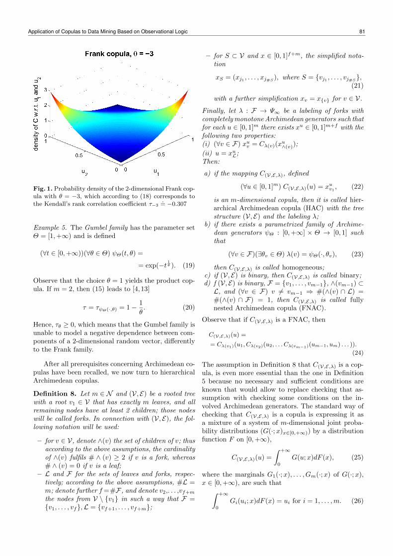
Fig. 1. Probability density of the 2-dimensional Frank cop-ula with θ = −3, which according to (18) corresponds tothe Kendall’s rank correlation coefficient τ−3

.= −0.307

Example 5. The Gumbel family has the parameter setΘ = [1,+∞) and is defined

(∀t ∈ [0,+∞))(∀θ ∈ Θ) ψΘ(t, θ) =

= exp(−t 1θ ). (19)

Observe that the choice θ = 1 yields the product cop-ula. If m = 2, then (15) leads to [4, 13]

τ = τψΘ(·,θ) = 1− 1

θ. (20)

Hence, τθ ≥ 0, which means that the Gumbel family isunable to model a negative dependence between com-ponents of a 2-dimensional random vector, differentlyto the Frank family.

After all prerequisites concerning Archimedean co-pulas have been recalled, we now turn to hierarchicalArchimedean copulas.

Definition 8. Let m ∈ N and (V, E) be a rooted treewith a root v1 ∈ V that has exactly m leaves, and allremaining nodes have at least 2 children; those nodeswill be called forks. In connection with (V, E), the fol-lowing notation will be used:

– for v ∈ V, denote ∧(v) the set of children of v; thusaccording to the above assumptions, the cardinalityof ∧(v) fulfils # ∧ (v) ≥ 2 if v is a fork, whereas# ∧ (v) = 0 if v is a leaf;

– L and F for the sets of leaves and forks, respec-tively; according to the above assumptions, #L =m; denote further f=#F , and denote v2,. . . ,vf+mthe nodes from V \ v1 in such a way that F =v1, . . . , vf,L = vf+1, . . . , vf+m;

– for S ⊂ V and x ∈ [0, 1]f+m, the simplified nota-tion

xS = (xj1 , . . . , xj#S ), where S = vj1 , . . . , vj#S,(21)

with a further simplification xv = xv for v ∈ V.Finally, let λ : F → Ψ∞ be a labeling of forks withcompletelymonotoneArchimedean generators such thatfor each u ∈ [0, 1]m there exists xu ∈ [0, 1]m+f with thefollowing two properties:(i) (∀v ∈ F) xuv = Cλ(v)(x

u∧(v));

(ii) u = xuL;Then:

a) if the mapping C(V,E,λ), defined

(∀u ∈ [0, 1]m) C(V,E,λ)(u) = xuv1 , (22)

is an m-dimensional copula, then it is called hier-archical Archimedean copula (HAC) with the treestructure (V, E) and the labeling λ;

b) if there exists a parametrized family of Archime-dean generators ψΘ : [0,+∞] × Θ → [0, 1] suchthat

(∀v ∈ F)(∃θv ∈ Θ) λ(v) = ψΘ(·, θv), (23)

then C(V,E,λ) is called homogeneous;c) if (V, E) is binary, then C(V,E,λ) is called binary;d) f (V, E) is binary, F = v1, . . . , vm−1, ∧(vm−1) ⊂L, and (∀v ∈ F) v 6= vm−1 ⇒ #(∧(v) ∩ L) =#(∧(v) ∩ F) = 1, then C(V,E,λ) is called fullynested Archimedean copula (FNAC).

Observe that if C(V,E,λ) is a FNAC, then

C(V,E,λ)(u) =

= Cλ(v1)(u1, Cλ(v2)(u2, . . . Cλ(vm−1)(um−1, um) . . . )).

(24)

The assumption in Definition 8 that C(V,E,λ) is a cop-ula, is even more essential than the one in Definition5 because no necessary and sufficient conditions areknown that would allow to replace checking that as-sumption with checking some conditions on the in-volved Archimedean generators. The standard way ofchecking that C(V,E,λ) is a copula is expressing it asa mixture of a system of m-dimensional joint proba-bility distributions (G(·;x)x∈[0,+∞)) by a distributionfunction F on [0,+∞),

C(V,E,λ)(u) =∫ +∞

0

G(u;x)dF (x), (25)

where the marginals G1(·;x), . . . , Gm(·;x) of G(·;x),x ∈ [0,+∞), are such that

∫ +∞

0

Gi(ui;x)dF (x) = ui for i = 1, . . . ,m. (26)

Application of Copulas to Data Mining Based on Observational Logic 81

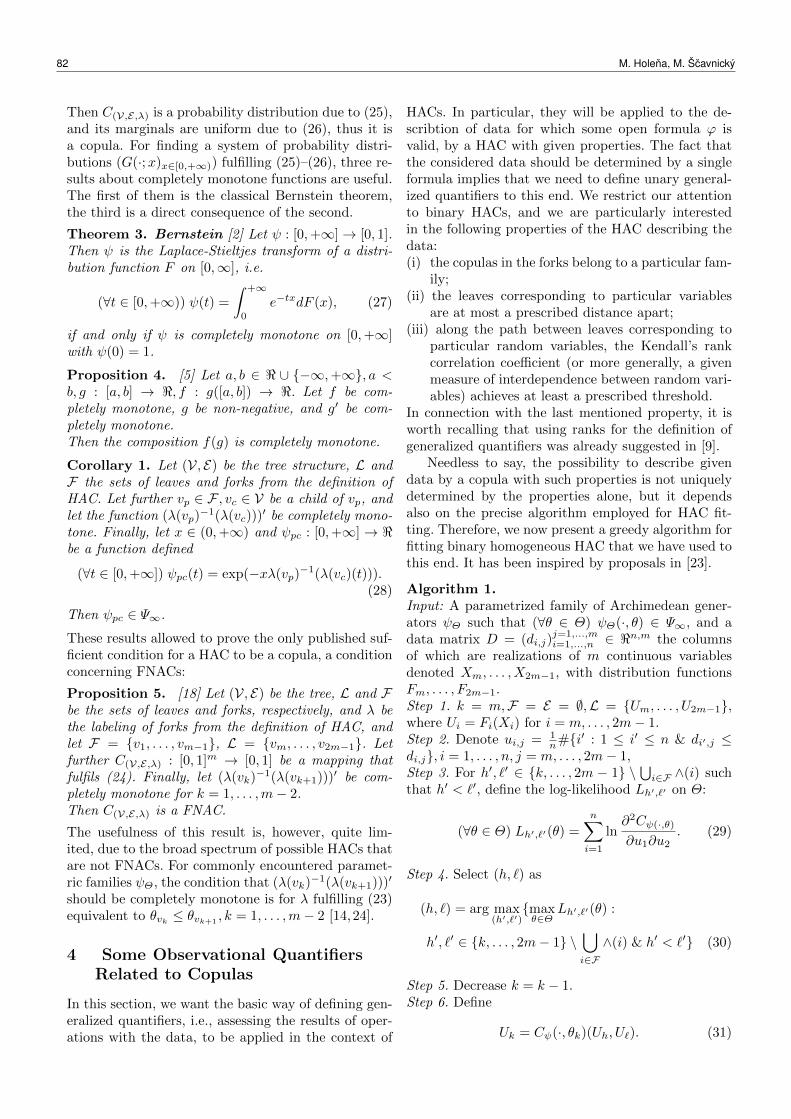
Then C(V,E,λ) is a probability distribution due to (25),and its marginals are uniform due to (26), thus it isa copula. For finding a system of probability distri-butions (G(·;x)x∈[0,+∞)) fulfilling (25)–(26), three re-sults about completely monotone functions are useful.The first of them is the classical Bernstein theorem,the third is a direct consequence of the second.

Theorem 3. Bernstein [2] Let ψ : [0,+∞]→ [0, 1].Then ψ is the Laplace-Stieltjes transform of a distri-bution function F on [0,∞], i.e.

(∀t ∈ [0,+∞)) ψ(t) =

∫ +∞

0

e−txdF (x), (27)

if and only if ψ is completely monotone on [0,+∞]with ψ(0) = 1.

Proposition 4. [5] Let a, b ∈ < ∪ −∞,+∞, a <b, g : [a, b] → <, f : g([a, b]) → <. Let f be com-pletely monotone, g be non-negative, and g′ be com-pletely monotone.Then the composition f(g) is completely monotone.

Corollary 1. Let (V, E) be the tree structure, L andF the sets of leaves and forks from the definition ofHAC. Let further vp ∈ F , vc ∈ V be a child of vp, andlet the function (λ(vp)

−1(λ(vc)))′ be completely mono-

tone. Finally, let x ∈ (0,+∞) and ψpc : [0,+∞] → <be a function defined

(∀t ∈ [0,+∞]) ψpc(t) = exp(−xλ(vp)−1(λ(vc)(t))).(28)

Then ψpc ∈ Ψ∞.

These results allowed to prove the only published suf-ficient condition for a HAC to be a copula, a conditionconcerning FNACs:

Proposition 5. [18] Let (V, E) be the tree, L and Fbe the sets of leaves and forks, respectively, and λ bethe labeling of forks from the definition of HAC, andlet F = v1, . . . , vm−1, L = vm, . . . , v2m−1. Letfurther C(V,E,λ) : [0, 1]m → [0, 1] be a mapping thatfulfils (24). Finally, let (λ(vk)

−1(λ(vk+1)))′ be com-

pletely monotone for k = 1, . . . ,m− 2.Then C(V,E,λ) is a FNAC.

The usefulness of this result is, however, quite lim-ited, due to the broad spectrum of possible HACs thatare not FNACs. For commonly encountered paramet-ric families ψΘ, the condition that (λ(vk)

−1(λ(vk+1)))′

should be completely monotone is for λ fulfilling (23)equivalent to θvk ≤ θvk+1

, k = 1, . . . ,m− 2 [14,24].

4 Some Observational QuantifiersRelated to Copulas

In this section, we want the basic way of defining gen-eralized quantifiers, i.e., assessing the results of oper-ations with the data, to be applied in the context of

HACs. In particular, they will be applied to the de-scribtion of data for which some open formula ϕ isvalid, by a HAC with given properties. The fact thatthe considered data should be determined by a singleformula implies that we need to define unary general-ized quantifiers to this end. We restrict our attentionto binary HACs, and we are particularly interestedin the following properties of the HAC describing thedata:(i) the copulas in the forks belong to a particular fam-

ily;(ii) the leaves corresponding to particular variables

are at most a prescribed distance apart;(iii) along the path between leaves corresponding to

particular random variables, the Kendall’s rankcorrelation coefficient (or more generally, a givenmeasure of interdependence between random vari-ables) achieves at least a prescribed threshold.

In connection with the last mentioned property, it isworth recalling that using ranks for the definition ofgeneralized quantifiers was already suggested in [9].

Needless to say, the possibility to describe givendata by a copula with such properties is not uniquelydetermined by the properties alone, but it dependsalso on the precise algorithm employed for HAC fit-ting. Therefore, we now present a greedy algorithm forfitting binary homogeneous HAC that we have used tothis end. It has been inspired by proposals in [23].

Algorithm 1.Input: A parametrized family of Archimedean gener-ators ψΘ such that (∀θ ∈ Θ) ψΘ(·, θ) ∈ Ψ∞, and adata matrix D = (di,j)

j=1,...,mi=1,...,n ∈ <n,m the columns

of which are realizations of m continuous variablesdenoted Xm, . . . , X2m−1, with distribution functionsFm, . . . , F2m−1.Step 1. k = m,F = E = ∅,L = Um, . . . , U2m−1,where Ui = Fi(Xi) for i = m, . . . , 2m− 1.Step 2. Denote ui,j = 1

n#i′ : 1 ≤ i′ ≤ n & di′,j ≤di,j, i = 1, . . . , n, j = m, . . . , 2m− 1,Step 3. For h′, `′ ∈ k, . . . , 2m − 1 \ ⋃i∈F ∧(i) suchthat h′ < `′, define the log-likelihood Lh′,`′ on Θ:

(∀θ ∈ Θ) Lh′,`′(θ) =n∑

i=1

ln∂2Cψ(·,θ)∂u1∂u2

. (29)

Step 4. Select (h, `) as

(h, `) = arg max(h′,`′)

maxθ∈Θ

Lh′,`′(θ) :

h′, `′ ∈ k, . . . , 2m− 1 \⋃

i∈F∧(i) & h′ < `′ (30)

Step 5. Decrease k = k − 1.Step 6. Define

Uk = Cψ(·, θk)(Uh, U`). (31)

82 M. Holena, M. Šcavnický

Step 7. Put

θk = maxθ∈Θ

Lh,`(θ), (32)

F = F ∪ Uk, (33)

E = E ∪ (Uk, Uh), (Uk, U`), (34)

λ(k) = ψ(·, θk). (35)

Step 8. If k > 1, denote ui,k = Cψ(·,θk)(ui,h, ui,`), i =1, . . . , n, and return to Step 3.Step 9. Else put V = L ∪ F and check whether themapping C(V,E,λ) defined by (22) is a copula, usingresults recalled in Section 3.Output: Rooted tree (V, E), mapping λ, informationwhether the mapping C(V,E,λ) is a copula (in positivecase, C(V,E,λ) is a HAC with the tree structure (V, E)and the labeling λ).

Once the HAC fitting algorithm is decided, we candefine new generalized quantifiers. Taking into accountthe above mentioned properties of binaryHAC inwhichwe are interested, we propose the following 3 quanti-fiers:

1. The quantifier HAC distance will be denoted

FamilyNameXm,...,X2m−1

i,L,j ,

where– FamilyName is the name of a parametrized

family of Archimedean generators to which thegenerators labeling the forks of the fitted HACbelong,

– Xm, . . . , X2m−1 are random variables from Al-gorithm 1,

– i, j ∈ m, . . . , 2m− 1,– L ∈ N , L ≥ 2.

The truth function of this quantifier is defined

(∀n ∈ N )(∀x = (x(1), . . . , x(n))′ ∈ 0, 1n,1)Tf

FamilyNameXm,...,X2m−1i,L,j

(x)=1 iff simultaneously

(36)

(i) #i : x(i) = 1 ≥ 1;(ii) according to the output of Algorithm 1, the map-

ping C(V,E,λ) is a copula;(iii) the path in (V, E) between the leaves Ui and Uj

has length ≤ L.2. The quantifier HAC Kendall’s τ will be denoted

FamilyNameXm,...,X2m−1

i,ϑ,j ,

where FamilyName, Xm, . . . , X2m−1 and i, j have thesame meaning as above, and ϑ ≥ 0. Its truth functionis defined

(∀n ∈ N )(∀x = (x(1), . . . , x(n))′ ∈ 0, 1n,1)Tf

FamilyNameXm,...,X2m−1i,ϑ,j

=1 iff simultaneously

(37)

(i) #i : x(i) = 1 ≥ 1;(ii) according to the output of Algorithm 1, the map-

ping C(V,E,λ) is a copula;(iii) for k ∈ F , if k is at the path from Ui to Uj , then

τψΘ(·,θk) ≥ ϑ.3. The quantifier HAC distance + Kendall’s τ will be

denoted

FamilyNameXm,...,X2m−1

i,L,ϑ,j ,

where FamilyName, Xm, . . . , X2m−1, i, j L and ϑ havethe same meaning as above. Its truth function is de-fined

(∀n ∈ N )(∀x = (x(1), . . . , x(n))′ ∈ 0, 1n,1)Tf

FamilyNameXm,...,X2m−1i,L,ϑ,j

(x) = 1 iff

TfFamilyName

Xm,...,X2m−1i,L,j

(x) =

= TfFamilyName

Xm,...,X2m−1i,ϑ,j

(x) = 1. (38)

5 Sketchy Results from Testing theNew Quantifiers

The proposed quantifiers were so far implemented onlyfor the Frank family of Archimedean generators. Thechoice of this family was due to the fact illustratedin Example 4, namely that binary copulas with gen-erators from this family can model also negative de-pendence between random variables. This is impor-tant, given some open formula ϕ, in view of the in-

terpretation of the closed formulas FrankXm,...,X2m−1

i,ϑ,j ϕ

and FrankXm,...,X2m−1

i,L,ϑ,j ϕ. The condition on the Ken-dall’s rank correlation coefficient, τψΘ(·,θk) ≥ ϑ ≥ 0for k ∈ F , is then a consequence of a positive depen-dence between the random variables corresponding tothe children of k, but not a consequence of an inabilityof the copula family to model a negative dependenceamong them, like it would be the case, e.g., for theGumbel family.

The implemented quantifiers were tested using 4data sets from the UCI repository of machine learningdata [31]: Iris, Seeds, Vertebral, Wine, as well as onemore data set from a recent real-world application incatalysis [21]. Due to space limitation, only sketchyresults for the best known among those data, the Irisdata set, will be shown [7].

In Figure 2, the tree structures of three HACs fit-ted to data fulfilling respectively the three open for-mulas Setosa, Versicolor and Virginica, as well asthe values of Kendall’s τ in their forks, are depicted.The leaves of the trees are X4= Sepal length, X5=Sepal width, X6= Petal length, X7= Petal width.Together with the information that each of the struc-tures indeed corresponds to a HAC, which was out-put from Algorithm 1, the tree structure already al-

lows to see which formulas FrankXm,...,X2m−1

i,L,j ϕ for L =

Application of Copulas to Data Mining Based on Observational Logic 83

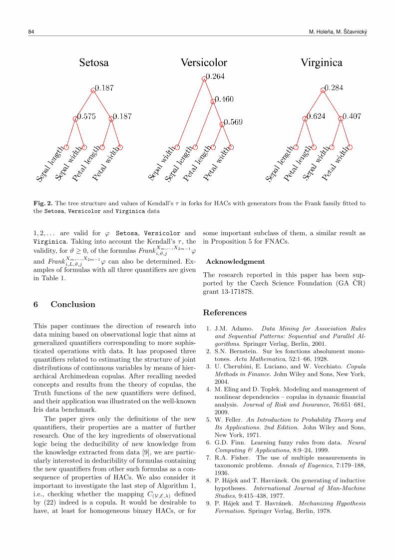
Fig. 2. The tree structure and values of Kendall’s τ in forks for HACs with generators from the Frank family fitted tothe Setosa, Versicolor and Virginica data

1, 2, . . . are valid for ϕ Setosa, Versicolor andVirginica. Taking into account the Kendall’s τ , the

validity, for ϑ ≥ 0, of the formulas FrankXm,...,X2m−1

i,ϑ,j ϕ

and FrankXm,...,X2m−1

i,L,ϑ,j ϕ can also be determined. Ex-amples of formulas with all three quantifiers are givenin Table 1.

6 Conclusion

This paper continues the direction of research intodata mining based on observational logic that aims atgeneralized quantifiers corresponding to more sophis-ticated operations with data. It has proposed threequantifiers related to estimating the structure of jointdistributions of continuous variables by means of hier-archical Archimedean copulas. After recalling neededconcepts and results from the theory of copulas, theTruth functions of the new quantifiers were defined,and their application was illustrated on the well-knownIris data benchmark.

The paper gives only the definitions of the newquantifiers, their properties are a matter of furtherresearch. One of the key ingredients of observationallogic being the deducibility of new knowledge fromthe knowledge extracted from data [9], we are partic-ularly interested in deducibility of formulas containingthe new quantifiers from other such formulas as a con-sequence of properties of HACs. We also consider itimportant to investigate the last step of Algorithm 1,i.e., checking whether the mapping C(V,E,λ) definedby (22) indeed is a copula. It would be desirable tohave, at least for homogeneous binary HACs, or for

some important subclass of them, a similar result asin Proposition 5 for FNACs.

Acknowledgment

The research reported in this paper has been sup-ported by the Czech Science Foundation (GA CR)grant 13-17187S.

References

1. J.M. Adamo. Data Mining for Association Rulesand Sequential Patterns: Sequential and Parallel Al-gorithms. Springer Verlag, Berlin, 2001.

2. S.N. Bernstein. Sur les fonctions absolument mono-tones. Acta Mathematica, 52:1–66, 1928.

3. U. Cherubini, E. Luciano, and W. Vecchiato. CopulaMethods in Finance. John Wiley and Sons, New York,2004.

4. M. Eling and D. Toplek. Modeling and management ofnonlinear dependencies – copulas in dynamic financialanalysis. Journal of Risk and Insurance, 76:651–681,2009.

5. W. Feller. An Introduction to Probability Theory andIts Applications. 2nd Edition. John Wiley and Sons,New York, 1971.

6. G.D. Finn. Learning fuzzy rules from data. NeuralComputing & Applications, 8:9–24, 1999.

7. R.A. Fisher. The use of multiple measurements intaxonomic problems. Annals of Eugenics, 7:179–188,1936.

8. P. Hajek and T. Havranek. On generating of inductivehypotheses. International Journal of Man-MachineStudies, 9:415–438, 1977.

9. P. Hajek and T. Havranek. Mechanizing HypothesisFormation. Springer Verlag, Berlin, 1978.

84 M. Holena, M. Šcavnický

Table 1. Example formulas obtainable from the tree structure and values of Kendall’s τ in Figure 2

FrankX4,...,X74,2,5 Setosa, but not FrankX4,...,X7

4,2,5 Versicolor neither FrankX4,...,X74,2,5 Virginica

FrankX4,...,X74,2,6 Virginica, but not FrankX4,...,X7

4,2,6 Setosa neither FrankX4,...,X74,2,6 Versicolor

FrankX4,...,X74,3,6 Versicolor and FrankX4,...,X7

4,3,6 Virginica, but not FrankX4,...,X74,3,5 Setosa

FrankX4,...,X74,0.5,5 Setosa, but not FrankX4,...,X7

4,0.5,5 Versicolor neither FrankX4,...,X74,0.5,5 Virginica

FrankX4,...,X76,0.5,7 Versicolor, but not FrankX4,...,X7

6,0.5,7 Setosa neither FrankX4,...,X76,0.5,7 Virginica

FrankX4,...,X74,0.6,6 Virginica, but not FrankX4,...,X7

4,0.6,6 Setosa neither FrankX4,...,X74,0.6,6 Versicolor

FrankX4,...,X74,2,0.5,5 Setosa, but not FrankX4,...,X7

4,2,0.5,5 Versicolor neither FrankX4,...,X74,2,0.5,5 Virginica

FrankX4,...,X74,3,0.4,7 Versicolor, but not FrankX4,...,X7

4,3,0.4,7 Setosa neither FrankX4,...,X74,3,0.4,7 Virginica

FrankX4,...,X75,2,0.4,7 Virginica, but not FrankX4,...,X7

5,2,0.4,7 Setosa neither FrankX4,...,X75,2,0.4,7 Versicolor

10. P. Hajek and M. Holena. Formal logics of discovery andhypothesis formation by machine. Theoretical Com-puter Science, 292:345–357, 2003.

11. P. Hajek, M. Holena, and J. Rauch. The guha methodand its meaning for data mining. Journal of Computerand System Sciences, 76:34–48, 2010.

12. D.J. Hand. Construction and Assessment of Classifi-cation Rules. John Wiley and Sons, New York, 1997.

13. JM. Hofert. Sampling Nested Archimedean Copulaswith Applications to CDO Pricing. PhD thesis, UlmUniversity, 2010.

14. J.M Hofert. A stochastic representation and samplingalgorithm for nested Archimedean copulas. Journalof Statistical Computation and Simulation, 82:1239–1255, 2012.

15. M. Holena. Fuzzy hypotheses for Guha implications.Fuzzy Sets and Systems, 98:101–125, 1998.

16. M. Holena. Fuzzy hypotheses testing in the frameworkof fuzzy logic. Fuzzy Sets and Systems, 145:229–252,2004.

17. H. Joe. Multivariate Models and Dependence Concepts.Chapman & Hall, London, 1997.

18. A.J. McNeil. Sampling nested archimedean copulas.Journal of Statistical Computation and Simulation,78:567–581, 2008.

19. A.J. McNeil and J. Neslehova. Multivariate Archi-medean copulas, d-monotone functions and l1-normsymmetric distributions. The Annals of Statistics,37:3059–3097, 2009.

20. S. Mitra and Y. Hayashi. Neuro-fuzzy rule generation:Survey in soft computing framework. IEEE Transac-tions on Neural Networks, 11:748–768, 2000.

21. S. Moehmel, N. Steinfeldt, S. Engelschalt, M. Holena,S. Kolf, U. Dingerdissen, D. Wolf, R. Weber, andM. Bewersdorf. New catalytic materials for thehigh-temperature synthesis of hydrocyanic acid frommethane and ammonia by high-throughput approach.Applied Catalysis A: General, 334:73–83, 2008.

22. R.B. Nelsen. An Introduction to Copulas. SpringerVerlag, Berlin, 2006.

23. O. Okhrin, Y. Okhrin, and W. Schmid. On the struc-ture and estimation of hierarchical Archimedean copu-las. Journal of Econometrics, 173:189–204, 2013.

24. O. Okhrin, Y. Okhrin, and W. Schmid. Properties ofhierarchical Archimedean copulas. Statistics & RiskModeling, 30:21–54, 2013.

25. K.M. Ramachandran. Mathematical Statistics withApplications. Elsevier Science Publishers, Amsterdam,2009.

26. J. Rauch and M. Simunek. Guha method and granularcomputing. In Proceedings of the IEEE Conference onGranular Computing, pages 630–635, 2005.

27. J. Rauch and M. Simunek. Action rules and the guhamethod: Preliminary considerations and results. In IS-MIS 2009 – Foundations of Intelligent Systems, pages76–87. Springer Verlag, Berlin, 2009.

28. J. Rauch, M. Simunek, and V. Lın. Mining for pat-terns based on contingency tables by kl-miner – firstexperience. In T.Y. Lin, X. Hu, S. Ohsuga, and C.J.Liau, editors, Data mining – Foundations and New Di-rections, pages 156–163, 2003.

29. Jan Rauch. Observational Calcucli and AssociationRules. Springer Verlag, Heidelberg, 2013.

30. A. Sklar. Fonctions de repartition a n dimensions etleur marges. Publications de l’Institut de Statistiquede l’Universit de Paris, 8:229–231, 1959.

31. University of California in Irwine,Machine LearningGroup. Repository of machine learning databases.http://www.ics.uci.edu/ mlearn/MLRepository.html.

32. C. Zhang and S. Zhang. Association Rule Mining.Models and Algorithms. Springer Verlag, Berlin, 2002.

Application of Copulas to Data Mining Based on Observational Logic 85

Improving the Model Guided Sampling Optimizationby Model Search and Slice Sampling

Lukáš Bajer1,2, Martin Holena2, and Viktor Charypar3

1 Faculty of Mathematics and Physics, Charles University in Prague,Malostranské nam. 25, 118 00 Prague 1, Czech Republic

bajer@cs.cas.cz2 Institute of Computer Science, Academy of Sciences of the Czech Republic,

Pod Vodárenskou veží 2, 182 07 Prague 8, Czech Republicmartin@cs.cas.cz

3 Faculty of Nuclear Sciences and Physical Engineering, Czech Technical University in Prague,Trojanova 13, 120 00 Prague 2, Czech Republic

charyvik@fjfi.cvut.cz

Abstract: Model Guided Sampling Optimization (MGSO)was recently proposed as an alternative for Jones’ Kriging-based EGO algorithm for optimization of expensive black-box functions. Instead of maximizing a chosen criterion(e.g., expected improvement), MGSO samples probabilityof improvement of the Gaussian process model formingmultiple candidates – a whole population of suggested so-lutions. This paper further develops this algorithm usingslice sampling method and continuous local optimizationof the Gaussian process model.

1 Introduction

Optimization of expensive empirical functions forms animportant topic in many engineering or natural-sciencesareas. For such functions, it is often impossible to obtainany derivatives or information about smoothness; more-over, there is no mathematical expression nor algorithm toevaluate. Instead, some simulation or experiment has to beperformed, and the measured value or result of such exper-iment is the value of the objective function being consid-ered. Such functions are also called black-box functions.They are usually very expensive to evaluate; one evalua-tion may cost a lot of time and money to process.

Because of the absence of the derivatives, standardcontinuous first- or second-order derivative optimizationmethods cannot be used. Further, functions of this kindare usually characterized by a high number of local optimawhere simple algorithms can be trapped easily. Therefore,different derivative-free optimization methods for black-box functions (often called meta-heuristics) have been pro-posed. Even though these methods are slow and computa-tionaly intensive, the cost of the evaluation of the empiri-cal objective function is always much higher, and so it iscructial to decrease the number of function evaluations asmuch as possible.

Evolutionary algorithms constitute a broad family ofmeta-heuristics that are used for black-box optimizationvery frequently. Some of these algorithms and techniquesare designed to minimize the number of objective func-

tion evaluations All of the three following approaches usea model (of a different type in each case), which is builtand updated within the optimization process.

Estimation of distribution algorithms (EDAs) [9] rep-resent one such approach: EDAs iteratively estimate theprobability distribution of selected candidate solutions(usually better than some threshold) and sample this distri-bution forming a new set of solutions for the next iteration.

Surrogate modelling is a technique of construction andusage of a regression model of the objective function [7].The model (called surrogate model in this context) is thenused to evaluate some of the candidate solutions instead ofevaluating them with the original costly function.

Our method, Model Guided Sampling Optimization(MGSO), takes inspiration from both these approaches. Ituses a regression model of the objective function, whichalso provides an error estimate. However, instead of re-placing the objective function with this model for someof the evaluations, it combines its prediction and the errorestimate to get a probability of reaching a better solutionin a given point. Similarly to EDAs, it then samples thispseudo-distribution1 to obtain the next set of solution can-didates.

The MGSO is similar to Jones’ Efficient Global Opti-mization (EGO) [8]. Where EGO selects a single solutionmaximizing a chosen criterion – Expected Improvement(EI) or Probability of Improvement (PoI) – the MGSOsamples the latter criterion. Hennig in his recent work [6]examines more criteria in detail. At the same time, the GPserves as a surrogate model of the objective function forsmall number of the solutions. In the second version ofMGSO, presented in this paper, this smooth optimizationis used in every generation of the optimization whereasthe previous version employed model optimization only toimprove the final optimum.

This paper extends the previous brief introduction ofMGSO [1]. Instead of Gibbs’ sampling, it uses slice sam-pling introduced by Neal [10]. This enables computa-

1a function proportional to a probability distribution, it’s value isgiven by the probability of improvement, see Section 2.2

ITAT 2013: Workshops, Posters, and Tutorials, pp. 86–91ISBN 978-1490952086, c© 2013 L. Bajer, M. Holena, V. Charypar

tionally cheaper sampling and works even in higher di-mensions where Gibbs’ sampling fails. Further, the GPmodel is used as a surrogate model more often, whichbrings faster convergence in the number of function evalu-ations. The following section introduces methods used inthe MGSO, Section 3 describes the MGSO algorithm, andSection 4 brings some preliminary results on the BBOBtesting set [4].

2 Involved Methods

2.1 Gaussian Processes

Gaussian process [12] is a probabilistic model based onGaussian distributions. This type of model was chosenbecause it predicts the function value in a new point inthe form of univariate Gaussian distribution: the mean andthe standard deviation of the function value are provided.Through the predicted mean, the GP can serve as a sur-rogate model, and the standard deviation is an estimate ofuncertainty of the prediction in a specified point.

The GP is specified by mean and covariance func-tions and relatively small number of covariance function’shyper-parameters. The hyper-parameters are fitted by themaximum-likelihood method.

Let XN = xi | xi ∈ RDNi=1 be a set of N training D-

dimensional data points with known dependent-variablevalues yN = yiN

i=1 and f (x) be an unknown function be-ing modelled for which f (xi) = yi for all i ∈ 1, . . . ,N.The GP model imposes a probabilistic model on the data:the vector of known function values yN is considered tobe a sample of a N-dimensional multivariate Gaussian dis-tribution with probability density p(yN |XN). If we takeinto consideration a new data point (xN+1,yN+1), the newprobability density is

p(yN+1 |XN+1) =exp(− 1

2 y>N+1C−1N+1yN+1)√

(2π)N+1 det(CN+1)(1)

where CN+1 is the covariance matrix of the Gaussian dis-tribution (for which mean is usually set to constant zero)and yN+1 = y1, . . . ,yN ,yN+1 (see [2] for details). Thiscovariance can be written as

CN+1 =

(CN kk> κ

)(2)

where CN is the covariance of the Gaussian distributiongiven the N training data points, k is a vector of covari-ances between the new point and training data, and κ isthe variance of the new point itself.

Predictions in Gaussian processes are made usingBayesian inference. Since the inverse C−1

N+1 of the ex-tended covariance matrix can be expressed using inverse ofthe training covariance C−1

N and yN is known, the densityof the distribution in a new point simplifies to a univariateGaussian with the density

p(yN+1 |XN+1,yN) ∝ exp

(−1

2(yN+1− yN+1)

2

s2yN+1

)(3)

with the mean and variance given by

yN+1 = k>C−1N yN , (4)

s2yN+1

= κ−k>C−1N k. (5)

Further details can be found in [2].The covariance CN plays a crucial role in these equa-

tions. It is defined by the covariance-function matrix Kand signal noise σ as

CN = KN +σIN (6)

where I is an identity matrix of order N. Gaussian pro-cesses use parametrized covariance functions K describ-ing prior assumptions on the shape of the modeled func-tion. The covariance between the function values at twodata points xi and x j is given by K(xi,x j), which formsthe (i, j)-th element of the matrix KN as well. In our case,we used the most common squared-exponential function

K(xi,x j) = θ exp(− 1

2`2 (xi−x j)>(xi−x j)

), (7)

which is suitable when the modelled function is rathersmooth. The closer the points xi and x j are, the closer thecovariance function value is to 1 and the stronger correla-tion between the function values f (xi) and f (x j) is. Thesignal variance θ scales this correlation, and the parameter` is the characteristic length-scale with which the distanceof two considered data points is compared. Our choiceof the covariance function was motivated by its simplicityand the possibility of finding the hyper-parameter valuesby the maximum-likelihood method.

2.2 Sampling

The core step of the MGSO algorithm is the sampling ofthe probability of improvement. This probability is, for achosen threshold T of the function value, directly givenby the predicted mean f (x) = y and the standard deviations(x) = sy of the GP model f in any point x of the inputspace

PoIT (x) = Φ(

T − f (x)s(x)

)= P( f (x)5 T ), (8)

which corresponds to the value of cumulative distribu-tion function (CDF) of the Gaussian with density (3) forthe value of threshold T . Even though all the variablescome from Gaussian distribution, PoI(x) is definitely notGaussian-shaped since it depends on the threshold T andthe function being modeled f – a typical example of thelandscape of PoI(x) in two dimensions for the Rastriginfunction is depicted in Fig. 1. The dependency on the mod-eled function also causes a lack of analytical marginals,derivatives or conditional probability densities.

Improving the Model Guided Sampling Optimization by Model Search and Slice Sampling 87

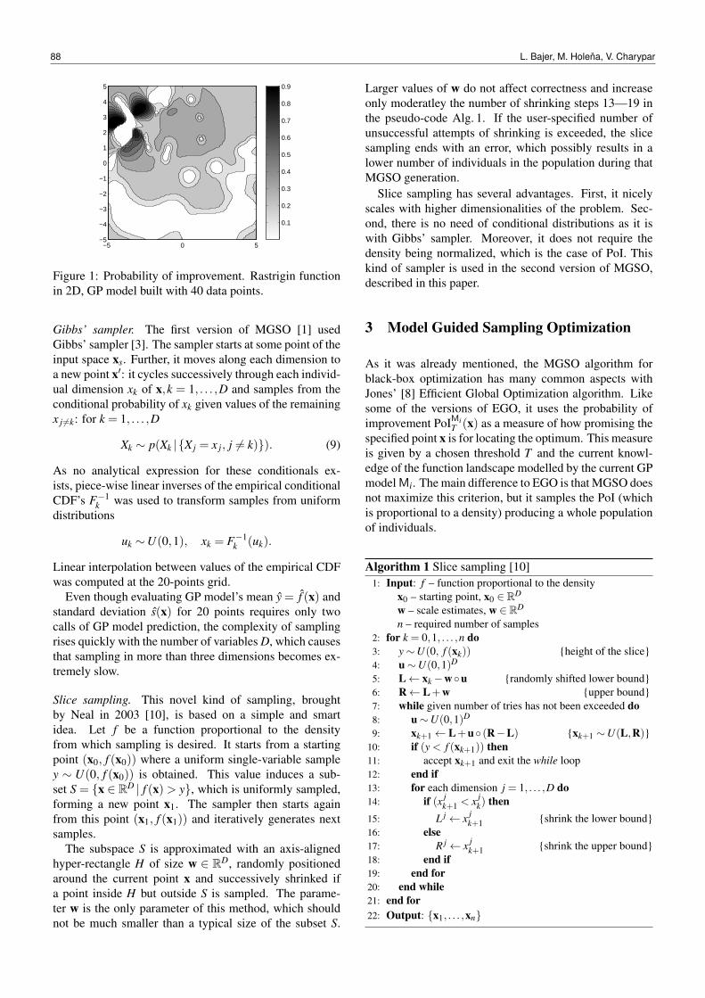
−5 0 5−5

−4

−3

−2

−1

0

1

2

3

4

5

0.1

0.2

0.3

0.4

0.5

0.6

0.7

0.8

0.9

Figure 1: Probability of improvement. Rastrigin functionin 2D, GP model built with 40 data points.

Gibbs’ sampler. The first version of MGSO [1] usedGibbs’ sampler [3]. The sampler starts at some point of theinput space xs. Further, it moves along each dimension toa new point x′: it cycles successively through each individ-ual dimension xk of x,k = 1, . . . ,D and samples from theconditional probability of xk given values of the remainingx j 6=k: for k = 1, . . . ,D

Xk ∼ p(Xk |X j = x j, j 6= k)). (9)

As no analytical expression for these conditionals ex-ists, piece-wise linear inverses of the empirical conditionalCDF’s F−1

k was used to transform samples from uniformdistributions

uk ∼U(0,1), xk = F−1k (uk).

Linear interpolation between values of the empirical CDFwas computed at the 20-points grid.

Even though evaluating GP model’s mean y = f (x) andstandard deviation s(x) for 20 points requires only twocalls of GP model prediction, the complexity of samplingrises quickly with the number of variables D, which causesthat sampling in more than three dimensions becomes ex-tremely slow.

Slice sampling. This novel kind of sampling, broughtby Neal in 2003 [10], is based on a simple and smartidea. Let f be a function proportional to the densityfrom which sampling is desired. It starts from a startingpoint (x0, f (x0)) where a uniform single-variable sampley ∼ U(0, f (x0)) is obtained. This value induces a sub-set S = x ∈ RD | f (x) > y, which is uniformly sampled,forming a new point x1. The sampler then starts againfrom this point (x1, f (x1)) and iteratively generates nextsamples.

The subspace S is approximated with an axis-alignedhyper-rectangle H of size w ∈ RD, randomly positionedaround the current point x and successively shrinked ifa point inside H but outside S is sampled. The parame-ter w is the only parameter of this method, which shouldnot be much smaller than a typical size of the subset S.

Larger values of w do not affect correctness and increaseonly moderatley the number of shrinking steps 13—19 inthe pseudo-code Alg. 1. If the user-specified number ofunsuccessful attempts of shrinking is exceeded, the slicesampling ends with an error, which possibly results in alower number of individuals in the population during thatMGSO generation.

Slice sampling has several advantages. First, it nicelyscales with higher dimensionalities of the problem. Sec-ond, there is no need of conditional distributions as it iswith Gibbs’ sampler. Moreover, it does not require thedensity being normalized, which is the case of PoI. Thiskind of sampler is used in the second version of MGSO,described in this paper.

3 Model Guided Sampling Optimization

As it was already mentioned, the MGSO algorithm forblack-box optimization has many common aspects withJones’ [8] Efficient Global Optimization algorithm. Likesome of the versions of EGO, it uses the probability ofimprovement PoIMi

T (x) as a measure of how promising thespecified point x is for locating the optimum. This measureis given by a chosen threshold T and the current knowl-edge of the function landscape modelled by the current GPmodel Mi. The main difference to EGO is that MGSO doesnot maximize this criterion, but it samples the PoI (whichis proportional to a density) producing a whole populationof individuals.

Algorithm 1 Slice sampling [10]1: Input: f – function proportional to the density

x0 – starting point, x0 ∈ RD

w – scale estimates, w ∈ RD

n – required number of samples2: for k = 0,1, . . . ,n do3: y∼U(0, f (xk)) height of the slice4: u∼U(0,1)D

5: L← xk−wu randomly shifted lower bound6: R← L+w upper bound7: while given number of tries has not been exceeded do8: u∼U(0,1)D

9: xk+1← L+u (R−L) xk+1 ∼U(L,R)10: if (y< f (xk+1)) then11: accept xk+1 and exit the while loop12: end if13: for each dimension j = 1, . . . ,D do14: if (x j

k+1 < x jk) then

15: L j← x jk+1 shrink the lower bound

16: else17: R j← x j

k+1 shrink the upper bound18: end if19: end for20: end while21: end for22: Output: x1, . . . ,xn

88 L. Bajer, M. Holena, V. Charypar

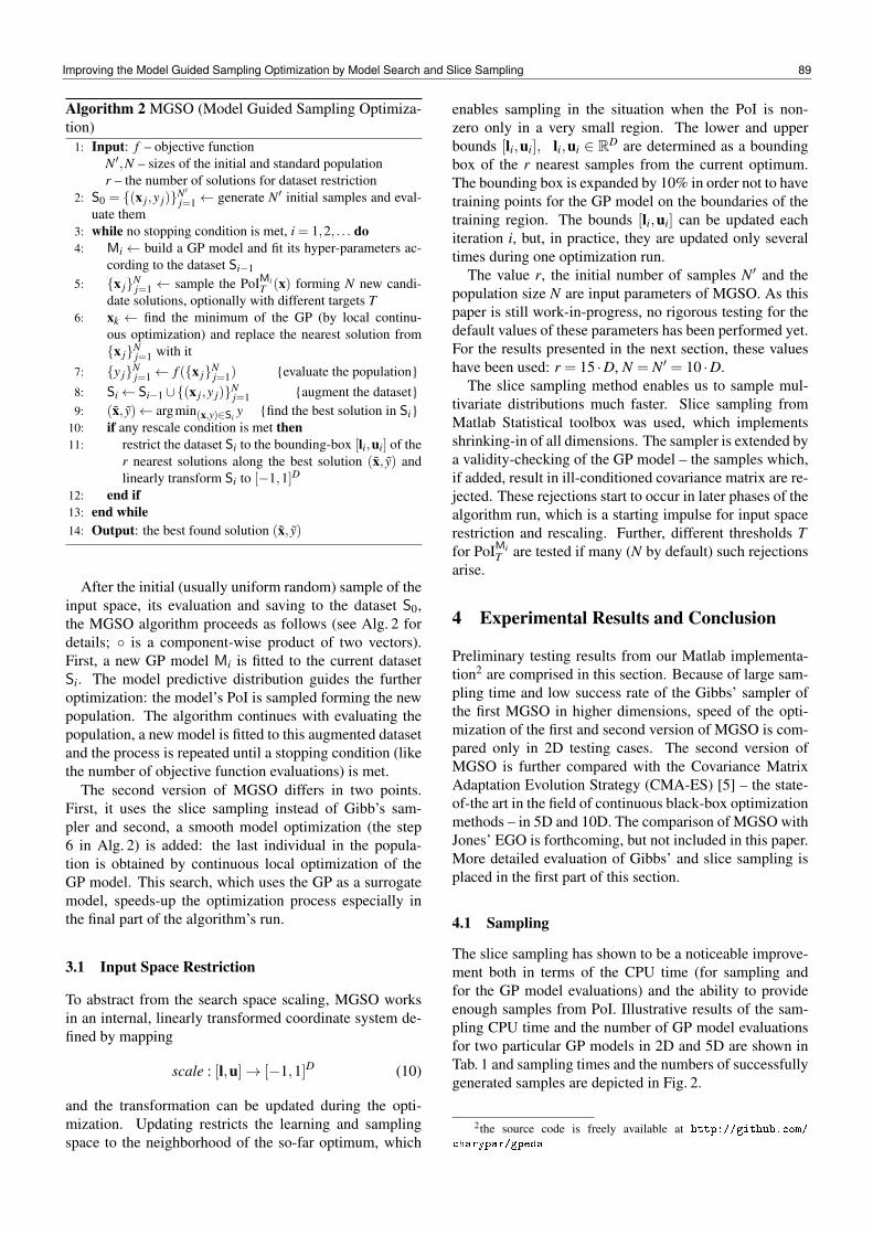
Algorithm 2 MGSO (Model Guided Sampling Optimiza-tion)

1: Input: f – objective functionN′,N – sizes of the initial and standard populationr – the number of solutions for dataset restriction

2: S0 = (x j,y j)N ′j=1← generate N′ initial samples and eval-

uate them3: while no stopping condition is met, i = 1,2, . . . do4: Mi ← build a GP model and fit its hyper-parameters ac-

cording to the dataset Si−1

5: x jNj=1 ← sample the PoIMi

T (x) forming N new candi-date solutions, optionally with different targets T

6: xk ← find the minimum of the GP (by local continu-ous optimization) and replace the nearest solution fromx jN

j=1 with it7: y jN

j=1← f (x jNj=1) evaluate the population

8: Si← Si−1∪(x j,y j)Nj=1 augment the dataset

9: (x, y)← argmin(x,y)∈Siy find the best solution in Si

10: if any rescale condition is met then11: restrict the dataset Si to the bounding-box [li,ui] of the

r nearest solutions along the best solution (x, y) andlinearly transform Si to [−1,1]D

12: end if13: end while14: Output: the best found solution (x, y)

After the initial (usually uniform random) sample of theinput space, its evaluation and saving to the dataset S0,the MGSO algorithm proceeds as follows (see Alg. 2 fordetails; is a component-wise product of two vectors).First, a new GP model Mi is fitted to the current datasetSi. The model predictive distribution guides the furtheroptimization: the model’s PoI is sampled forming the newpopulation. The algorithm continues with evaluating thepopulation, a new model is fitted to this augmented datasetand the process is repeated until a stopping condition (likethe number of objective function evaluations) is met.

The second version of MGSO differs in two points.First, it uses the slice sampling instead of Gibb’s sam-pler and second, a smooth model optimization (the step6 in Alg. 2) is added: the last individual in the popula-tion is obtained by continuous local optimization of theGP model. This search, which uses the GP as a surrogatemodel, speeds-up the optimization process especially inthe final part of the algorithm’s run.

3.1 Input Space Restriction

To abstract from the search space scaling, MGSO worksin an internal, linearly transformed coordinate system de-fined by mapping

scale : [l,u]→ [−1,1]D (10)

and the transformation can be updated during the opti-mization. Updating restricts the learning and samplingspace to the neighborhood of the so-far optimum, which

enables sampling in the situation when the PoI is non-zero only in a very small region. The lower and upperbounds [li,ui], li,ui ∈ RD are determined as a boundingbox of the r nearest samples from the current optimum.The bounding box is expanded by 10% in order not to havetraining points for the GP model on the boundaries of thetraining region. The bounds [li,ui] can be updated eachiteration i, but, in practice, they are updated only severaltimes during one optimization run.

The value r, the initial number of samples N′ and thepopulation size N are input parameters of MGSO. As thispaper is still work-in-progress, no rigorous testing for thedefault values of these parameters has been performed yet.For the results presented in the next section, these valueshave been used: r = 15 ·D, N = N′ = 10 ·D.

The slice sampling method enables us to sample mul-tivariate distributions much faster. Slice sampling fromMatlab Statistical toolbox was used, which implementsshrinking-in of all dimensions. The sampler is extended bya validity-checking of the GP model – the samples which,if added, result in ill-conditioned covariance matrix are re-jected. These rejections start to occur in later phases of thealgorithm run, which is a starting impulse for input spacerestriction and rescaling. Further, different thresholds Tfor PoIMi

T are tested if many (N by default) such rejectionsarise.

4 Experimental Results and Conclusion

Preliminary testing results from our Matlab implementa-tion2 are comprised in this section. Because of large sam-pling time and low success rate of the Gibbs’ sampler ofthe first MGSO in higher dimensions, speed of the opti-mization of the first and second version of MGSO is com-pared only in 2D testing cases. The second version ofMGSO is further compared with the Covariance MatrixAdaptation Evolution Strategy (CMA-ES) [5] – the state-of-the art in the field of continuous black-box optimizationmethods – in 5D and 10D. The comparison of MGSO withJones’ EGO is forthcoming, but not included in this paper.More detailed evaluation of Gibbs’ and slice sampling isplaced in the first part of this section.

4.1 Sampling

The slice sampling has shown to be a noticeable improve-ment both in terms of the CPU time (for sampling andfor the GP model evaluations) and the ability to provideenough samples from PoI. Illustrative results of the sam-pling CPU time and the number of GP model evaluationsfor two particular GP models in 2D and 5D are shown inTab. 1 and sampling times and the numbers of successfullygenerated samples are depicted in Fig. 2.

2the source code is freely available at http://github.com/

charypar/gpeda

Improving the Model Guided Sampling Optimization by Model Search and Slice Sampling 89

Table 1: Comparison of Gibbs’ and Slice sampling, re-sults from 15 runs of sampling. Average CPU time andthe number of evaluations of the GP model’s PoI neededto generate 20/50 samples in 2D/5D. The differences ofthe CPU time per GP evaluation is mainly because of thebatch evaluation of PoI for empir. CDF in Gibbs’ sampler.

Gibbs 2D slice 2D Gibbs 5D slice 5Dtime [s] 1.85 1.11 42.41 17.56# GP eval. 2 402 246 20 087 2 909

Gibbs slice0

10

20

30

40

50

60

70

80

time

[s]

Gibbs slice0

10

20

30

40

50

num

ber

of g

ener

ated

sam

ples

Figure 2: Computational time and the number of success-fully generated samples in 5D. Results from 15 indepen-dent runs with the same GP model/PoI.

4.2 BBOB Benchmark Functions Optimization

The proposed MGSO has been tested on three differentcontinuous benchmark functions from the BBOB testingset [4]: sphere, Rosenbrock and Rastrigin functions. Al-though the previous version of the algorithm [1] was prac-tically able to optimize only two-dimensional versions ofthese functions, this paper provides results from 5D and10D as well. The computational speed-up was causedmainly by the slice sampling method and partly also bythe continuous model optimization step.

In two dimensions, the current version of the MGSOoutperformed CMA-ES (considering budget 500 originalevaluations) on both sphere and Rosenbrock functions,and it performs approximately equally well on Rastriginfunction, see Fig. 3. In terms of the CPU time for thewhole optimization, the CMA-ES runs in several secondswhile MGSO takes several or tens of minutes to pro-cess. But as we are concerned with expensive (usuallyempirical-function) optimization, we suppose the cost forthe MGSO search being dominated by the time and moneyfor the original evaluations.

The MGSO scales nicely on the unimodal and sym-metric sphere function. Both in 5D and 10D, a dramat-ically lower number of function evaluations is needed toreach threshold of the objective function values f∆ = 10−4

than in the case of CMA-ES, see Fig. 4 and Fig. 5. Onthe Rosenbrock function, however, the number of evalua-tions of MGSO needed to reach f∆ = 10−2 is lower in 5D,

0 200 40010

−8

10−6

10−4

10−2

100

102

104

f ∆

# of function eval.

Sphere in 2D

0 200 40010

−8

10−6

10−4

10−2

100

102

104

f ∆

# of function eval.

Rosenbrock in 2D

0 200 40010

−8

10−6

10−4

10−2

100

102

104

f ∆

# of function eval.

Rastrigin in 2D

MGSO v. 1MGSO v. 2CMA−ES

MGSO v. 1MGSO v. 2CMA−ES

MGSO v. 1MGSO v. 2CMA−ES

Figure 3: 2-D. Medians of the best found function valuesgathered from 15 independent runs. The First [1] and thesecond version of MGSO are compared with CMA-ES.

0 500 1000

10−4

10−3

10−2

10−1

100

101

102

103

104

f ∆

# of function eval.

Sphere in 5D

0 500 1000

10−4

10−3

10−2

10−1

100

101

102

103

104

f ∆

# of function eval.

Rosenbrock in 5D

0 500 1000

10−4

10−3

10−2

10−1

100

101

102

103

104

f ∆# of function eval.

Rastrigin in 5D

MGSO v. 2CMA−ES

MGSO v. 2CMA−ES

MGSO v. 2CMA−ES

Figure 4: 5-D. Medians of the best found function valuesgathered from 15 runs. The second version of MGSO iscompared to CMA-ES.

0 1000 200010

−4

10−3

10−2

10−1

100

101

102

103

104

105

f ∆

# of function eval.

Sphere in 10D

0 1000 200010

−4

10−3

10−2

10−1

100

101

102

103

104

105

f ∆

# of function eval.

Rosenbrock in 10D

0 1000 200010

−4

10−3

10−2

10−1

100

101

102

103

104

105

f ∆

# of function eval.

Rastrigin in 10D

MGSO v. 2CMA−ES

MGSO v. 2CMA−ES

MGSO v. 2CMA−ES

Figure 5: 5-D. Medians of the best found function valuesgathered from 15 runs. The second version of MGSO iscompared to CMA-ES.

90 L. Bajer, M. Holena, V. Charypar

but CMA-ES works better in 10D. The multimodal Ras-trigin function with large number of local minima is notharder than the two other functions for CMA-ES, but it isnot the case of the MGSO. Our algorithm is outperformedby CMA-ES in both 5D and 10D for that benchmark func-tion.

4.3 Conclusions and future work

Our method shows promising results in terms of the num-ber of true objective function evaluations in the initialphase of optimization. However, there are still many is-sues to solve. In general, we are planning to work on im-proving the final local optimization in the region of the op-timum either by improving MGSO itself or combining itwith some other method in the final phase. Further, fittingof the hyper-parameters of the GP model will be studied,since GPML implementation3 [11] being used is often notable to fit them to optimal values.

Future work should also test different initial samplingschemes, which affect the model quality and thus perfor-mance of the method, and perform rigorous testing of theeffects of input parameters, which were set by hand for ourinitial experiments. A comparison with the EGO method,which was not done due to a lack of a readily availableimplementation, will also be performed.

The Model Guided Sampling Optimization was intro-duced in more detail. Several improvements of this algo-rithm were given and more experimental results than in thelast brief work [1] were provided. The experiments showthat the proposed method can successfully compete withthe state-of-the art continuous black-box optimization al-gorithm CMA-ES in lower dimensions and on unimodalsymmetric functions.

Acknowledgments

This work was supported by the Czech ScienceFoundation (GACR) grants P202/11/1368 and13-17187S, the Grant Agency of the Charles Uni-versity (GAUK) 278511/2011 grant and the Grant Agencyof the Czech Technical University in Prague, grantNo. SGS12/196/OHK3/3T/14.

References

[1] L. Bajer, V. Charypar, and M. Holena. Model guided sam-pling optimization with gaussian processes for expensiveblack-box optimization. In GECCO ’13 Proceedings, Am-sterdam, Netherlands, 2013. ACM, New York.

[2] D. Buche, N. Schraudolph, and P. Koumoutsakos. Acceler-ating evolutionary algorithms with gaussian process fitnessfunction models. IEEE Transactions on Systems, Man, andCybernetics, Part C: Applications and Reviews, 35(2):183–194, 2005.

3http://www.gaussianprocess.org/gpml/code/matlab/

[3] S. Geman and D. Geman. Stochastic relaxation, Gibbs dis-tributions, and the Bayesian restoration of images. IEEETransactions on Pattern Analysis and Machine Intelli-gence, PAMI-6(6):721–741, 1984.

[4] N. Hansen, S. Finck, R. Ros, and A. Auger. Real-parameterblack-box optimization benchmarking 2009: Noiselessfunctions definitions. Technical Report RR-6829, INRIA,2009. Updated February 2010.

[5] N. Hansen and A. Ostermeier. Completely derandomizedself-adaptation in evolution strategies. Evolutionary Com-putation, 9(2):159–195, June 2001.

[6] P. Hennig and C. J. Schuler. Entropy search forinformation-efficient global optimization. J. Mach. Learn.Res., 13:1809–1837, June 2012.

[7] Y. Jin. A comprehensive survey of fitness approximation inevolutionary computation. Soft Computing, 9(1):3–12, Jan.2005.

[8] D. R. Jones, M. Schonlau, and W. J. Welch. Efficient globaloptimization of expensive black-box functions. Journal ofGlobal Optimization, 13(4):455–492, Dec. 1998.

[9] P. Larrañaga and J. A. Lozano. Estimation of distribu-tion algorithms: A new tool for evolutionary computation.Kluwer, 2002.

[10] R. M. Neal. Slice sampling. The Annals of Statistics,31(3):705–767, June 2003.

[11] C. E. Rasmussen and H. Nickisch. Gaussian processes formachine learning (GPML) toolbox. J. Mach. Learn. Res.,11:3011–3015, Dec. 2010.

[12] C. E. Rasmussen and C. K. I. Williams. Gaussian Pro-cesses for Machine Learning. Adaptative computation andmachine learning series. MIT Press, 2006.

Improving the Model Guided Sampling Optimization by Model Search and Slice Sampling 91

Design and comparison of two rule-based fuzzy classifiers for computersecurity

Martin Kopp1,2, Martin Holena2

1 Faculty of Information Technology, Czech Technical University in PragueThákurova 9, 160 00 Prague

2 Institute of Computer Science, Academy of Sciences of the Czech RepublicPod Vodárenskou veží 2, 182 07 Prague

Abstract: This paper describes the design and comparisonof two rule based fuzzy classifiers, which are subsequentlyenhanced with respect to comprehensibility. The firstapproach is based on random forests. The second is aspecific kind of a fuzzy decision tree which is built oninformation granules extracted from results of a fuzzyclustering algorithm. Membership functions of fuzzysets are fitted to the outputs of these two tree basedclassifiers. This gives us logical rules, which have a bettercomprehensibility. These two approaches are comparedto each other and with a support vector machine classifieras a representative of precise classifiers. The comparisonis performed on data concerning network security.

Keywords: Comprehensible classification, decisiontree, fuzzy clustering, random forest, rule-based classifi-cation.

1 Introduction

There are two main lines of study in an intrusion detection:misuse detection [25] and anomaly detection [1]. Signa-ture based misuse detection methods, of course, can rec-ognize well known attacks only. The anomaly detectionis focused on finding unusual activities [5][13][22]. Thismethod is still less accurate in revealing known patterns,but superior in the way it can detect novelty attacks. Re-cently, an intrusion detection attracted many researchersfrom machine learning [3][14][18].

Machine learning techniques for an intrusion detectioncan be divided into to two groups with different goals, de-sign of more accurate systems [17] and design or improve-ment of such systems to achieve better comprehensibility[19]. This paper is focused on the second goal and com-pares two methods, how to build up rule-based a fuzzyclassifier focused on comprehensibility. The first one isbased on an ensemble of decision trees [24] and referred toas the random forest method. The second one, based on in-formation granules extracted from data by fuzzy c-meansalgorithm, will be called C-Fuzzy decision tree. For moreinformation about fuzzy systems and fuzzy classification,we refer to [10][11][12].

This paper is organized as follows. Section 2 providesan overview of the random forest based method. In section

3, the C-Fuzzy decision tree method will be described, fol-lowed by the process of fitting fuzzy sets to the output insection 4. Section 5 describes experiments on the KDD 99data set [9].

2 Random forest based method

Decision trees [23] are commonly used in machine learn-ing and classification. Each inner node j of the tree storesa binary split function:

h(V,θ j) ∈ 0,1, (1)

in which θ = (φ ,ψ,τ), where φ is a filter function, whichchooses some features from a whole feature space V, ψdefines a geometric primitive used to separate data (e.g.hyperplane) and τ is a vector of thresholds for inequalitiesused in binary tests. The leaf nodes then store class labels.The tree is built up (grown) by splitting nodes with highheterogeneity criterion such as entropy, Gini index [6] etc.

Compared to other machine learning methods, decisiontrees have many advantages like robustness, handling bothnumerical and categorical data, and finally, trees are easyto understand and interpret. In recent years, ensembles ofclassifiers became most popular due to their greater accu-racy and generalization ability. Decision trees are no ex-ceptions and ensembles of them are called decision forests.

In this paper we work with random decision forests.This method has been introduced in [7]. The random na-ture of the forest can be achieved by a random featuresselection or random sampling of a training dataset. Thesetwo techniques are not mutually exclusive and can be usedtogether. For more detailed description of random forestsand their application, we refer to [4].

The training of a tree is done by optimizing parametersof (1) at each split node j via:

θ ∗j = argmaxθ j

I j (2)

For classification, the objective function I j takes the formof an information gain defined as:

I j = H(S j)− ∑i∈L,R

|Sij||S j|

H(Sij), (3)

ITAT 2013: Workshops, Posters, and Tutorials, pp. 92–99ISBN 978-1490952086, c© 2013 M. Kopp, M. Holena

with S j as a set of data points at the current node andi indexing its child nodes (left,right). The entropy for ageneric set S is defined as:

H(S) =−∑c∈C

p(c)logp(c) (4)

where c is a class label such that c ∈ C and C is a set ofall classes. The p(c) is a prior probability of c and in ourimplementation it is calculated as a normalized empiricalhistogram of labels corresponding to training points in S.

Classification forests produce a probabilistic class dis-tribution. In fact, each tree leaf yields a posterior proba-bility pt(c|V). So the forest output is typically given by:

p(c|V) =1T

T

∑t

pt(c|V) (5)

where t ∈ T .The properties of the forest, like accuracy and general-

ization, depend on several parameters:

• The forest size T.

• The maximal tree depth D.

• The proportion ρ of randomly chosen features fromthe whole feature space V.

How each of them influences the forest prediction abil-ity, will be discussed in section 5.

3 C-Fuzzy Decision tree

Standard decision trees have several limitations. At thefirst place, only the most discriminative attribute is chosento be split, in each inner node. Secondly, before forestsemerged, decision trees were crisp predictors. There wasno membership grade or a class distribution. The cluster-oriented decision trees are a new kind of decision treesthat attempt to overcome these limitations by perceivingdata as a collection of information granules [20]. Infor-mation granules are almost synonym of clusters [8]. Fur-thermore, fuzzy granulations help to model soft boundsamongst classes, instead of crisp ones, what leads to bet-ter approximation of real bounds. It is evident now thatfuzzy clusters are the central concept behind the general-ized trees. They will be referred to as C-Fuzzy decisiontrees [21].

3.1 Overall structure of C-Fuzzy trees

The whole process of growing the tree is pretty simple andcan be summarized in the following steps:

1. Run a fuzzy clustering and assign results to nodes.

2. Find a node Ni with the highest heterogeneity Vi.

3. Perform a fuzzy clustering over patterns of the node Ni.

4. Split the node Ni and assign clusters to new nodes.

5. If a stopping condition is fulfilled, end, else return to 2.

Typical stopping conditions are: a heterogeneity crite-rion falls under a threshold, the number of patterns as-signed to the node is smaller than some value etc. Whensplit, each node is divided to exactly c clusters. Lowervalues of c, like c = 2 or c = 3, produce deep trees, wherehigher c, like c = 7, produce broader trees instead.

3.2 Fuzzy clustering

A fuzzy clustering is the most important part of buildingthe tree, it provides a full description of nodes. For thepurpose of this paper, the fuzzy C-means (FCM) was se-lected as a well known and documented algorithm [2]. Inthe FCM algorithm, the clusters are build trough minimal-ization of some objective function. The standard objectivefunction Q assumes the format:

Q =c

∑i=1

N

∑k=1

uγikd2

ik (6)

where U = [uik], i = 1,2, ...,c,k = 1,2, ....,N is a partitionmatrix, c is the number of clusters, N is the number ofdata points, γ is a fuzzification factor (usually γ = 2) anddik stands for the distance between the ith prototype andthe kth data point. In our implementation, the data pointscome in the ordered pairs (x(k),y(k)), where x(k) standsfor the input vector of the kth data point and y(k) is itscorresponding output. For the clustering, these pairs areconcatenated into vectors:

z(k) = [x1(k)x2(k)...xn(k)y(k)] (7)

where n is the number of features. This implies that theclustering is done in a (n+1) dimensional space and aresulting prototype fi is positioned in Rn+1. The FCMalgorithm starts from randomly generated prototypes andachieves optimization task by iterating following steps:

partition update

uik =1

∑cj=1(

dikd jk

)2/(γ−1)(8)

where dik is some distance of the ith prototype fi and thekth data point xk, typically Euclidean.

prototype update

fnewi =

∑Nk=1 uγ

ikzk

∑Nk=1 uγ

ik(9)

If we denote the number of clusters c and split themd-times then then number of nodes will be c ∗ d. But theclassification is performed only in leaf nodes. There ared(c−1)+1 of them. Therefore, a new data point is com-pared to d(c− 1)+ 1 prototypes and then assigned to thecluster corresponding to the most similar one.

Design and Comparison of Two Rule-based Fuzzy Classifiers for Computer Security 93

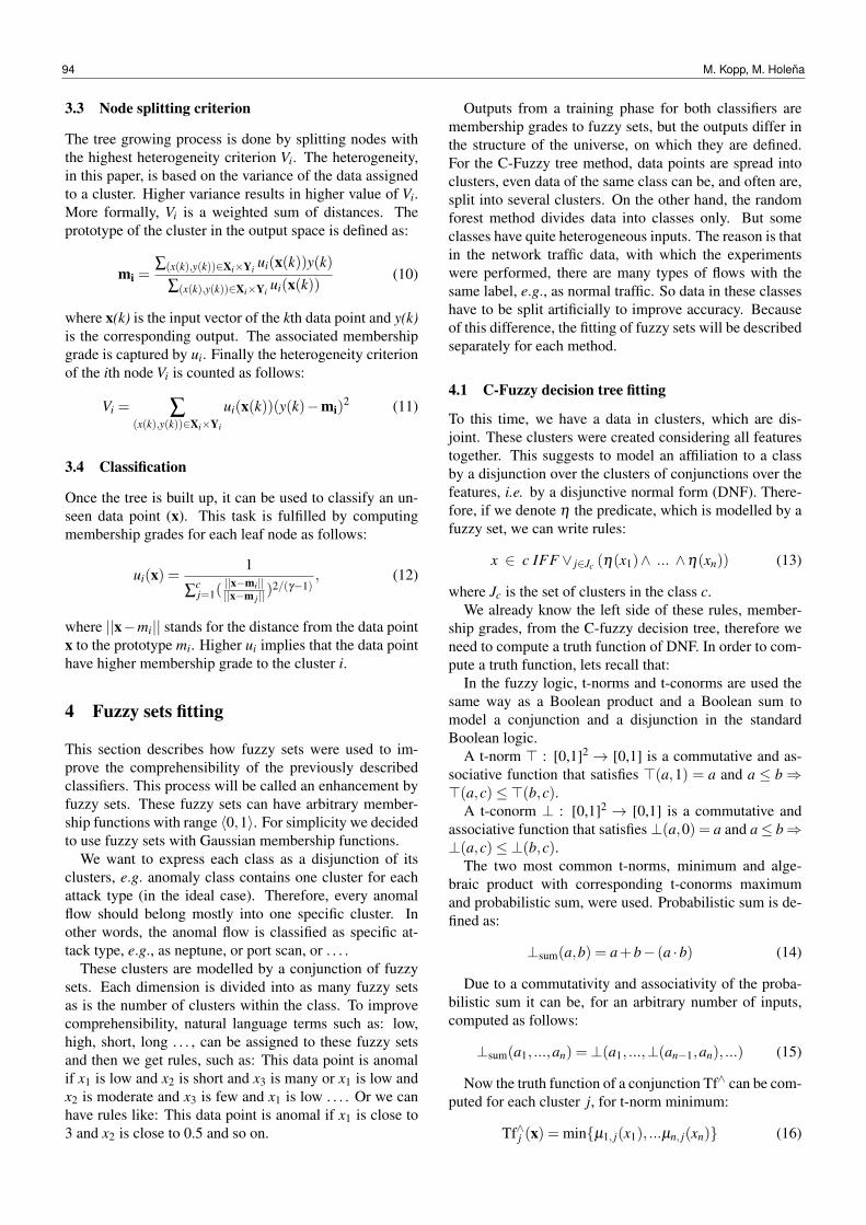
3.3 Node splitting criterion

The tree growing process is done by splitting nodes withthe highest heterogeneity criterion Vi. The heterogeneity,in this paper, is based on the variance of the data assignedto a cluster. Higher variance results in higher value of Vi.More formally, Vi is a weighted sum of distances. Theprototype of the cluster in the output space is defined as:

mi =∑(x(k),y(k))∈Xi×Yi ui(x(k))y(k)

∑(x(k),y(k))∈Xi×Yi ui(x(k))(10)

where x(k) is the input vector of the kth data point and y(k)is the corresponding output. The associated membershipgrade is captured by ui. Finally the heterogeneity criterionof the ith node Vi is counted as follows:

Vi = ∑(x(k),y(k))∈Xi×Yi

ui(x(k))(y(k)−mi)2 (11)

3.4 Classification

Once the tree is built up, it can be used to classify an un-seen data point (x). This task is fulfilled by computingmembership grades for each leaf node as follows:

ui(x) =1

∑cj=1(

||x−mi||||x−m j || )

2/(γ−1), (12)

where ||x−mi|| stands for the distance from the data pointx to the prototype mi. Higher ui implies that the data pointhave higher membership grade to the cluster i.

4 Fuzzy sets fitting

This section describes how fuzzy sets were used to im-prove the comprehensibility of the previously describedclassifiers. This process will be called an enhancement byfuzzy sets. These fuzzy sets can have arbitrary member-ship functions with range 〈0,1〉. For simplicity we decidedto use fuzzy sets with Gaussian membership functions.

We want to express each class as a disjunction of itsclusters, e.g. anomaly class contains one cluster for eachattack type (in the ideal case). Therefore, every anomalflow should belong mostly into one specific cluster. Inother words, the anomal flow is classified as specific at-tack type, e.g., as neptune, or port scan, or . . . .

These clusters are modelled by a conjunction of fuzzysets. Each dimension is divided into as many fuzzy setsas is the number of clusters within the class. To improvecomprehensibility, natural language terms such as: low,high, short, long . . . , can be assigned to these fuzzy setsand then we get rules, such as: This data point is anomalif x1 is low and x2 is short and x3 is many or x1 is low andx2 is moderate and x3 is few and x1 is low . . . . Or we canhave rules like: This data point is anomal if x1 is close to3 and x2 is close to 0.5 and so on.

Outputs from a training phase for both classifiers aremembership grades to fuzzy sets, but the outputs differ inthe structure of the universe, on which they are defined.For the C-Fuzzy tree method, data points are spread intoclusters, even data of the same class can be, and often are,split into several clusters. On the other hand, the randomforest method divides data into classes only. But someclasses have quite heterogeneous inputs. The reason is thatin the network traffic data, with which the experimentswere performed, there are many types of flows with thesame label, e.g., as normal traffic. So data in these classeshave to be split artificially to improve accuracy. Becauseof this difference, the fitting of fuzzy sets will be describedseparately for each method.

4.1 C-Fuzzy decision tree fitting

To this time, we have a data in clusters, which are dis-joint. These clusters were created considering all featurestogether. This suggests to model an affiliation to a classby a disjunction over the clusters of conjunctions over thefeatures, i.e. by a disjunctive normal form (DNF). There-fore, if we denote η the predicate, which is modelled by afuzzy set, we can write rules:

x ∈ c IFF ∨ j∈Jc (η(x1)∧ ... ∧η(xn)) (13)

where Jc is the set of clusters in the class c.We already know the left side of these rules, member-

ship grades, from the C-fuzzy decision tree, therefore weneed to compute a truth function of DNF. In order to com-pute a truth function, lets recall that:

In the fuzzy logic, t-norms and t-conorms are used thesame way as a Boolean product and a Boolean sum tomodel a conjunction and a disjunction in the standardBoolean logic.

A t-norm > : [0,1]2 → [0,1] is a commutative and as-sociative function that satisfies >(a,1) = a and a ≤ b⇒>(a,c)≤>(b,c).

A t-conorm ⊥ : [0,1]2 → [0,1] is a commutative andassociative function that satisfies⊥(a,0) = a and a≤ b⇒⊥(a,c)≤⊥(b,c).

The two most common t-norms, minimum and alge-braic product with corresponding t-conorms maximumand probabilistic sum, were used. Probabilistic sum is de-fined as:

⊥sum(a,b) = a+b− (a ·b) (14)

Due to a commutativity and associativity of the proba-bilistic sum it can be, for an arbitrary number of inputs,computed as follows:

⊥sum(a1, ...,an) =⊥(a1, ...,⊥(an−1,an), ...) (15)

Now the truth function of a conjunction Tf∧ can be com-puted for each cluster j, for t-norm minimum:

Tf∧j (x) = minµ1, j(x1), ...µn, j(xn) (16)

94 M. Kopp, M. Holena

and for algebraic product:

Tf∧j (x) = µ1, j(x1) · ... ·µn, j(xn), (17)

where µ js are membership grades of the individual dimen-sions of the data point x to fuzzy sets, which are modelledby one dimensional Gaussians, as was mentioned above.

For each cluster, the truth function of the conjunctionTf∧ is fitted by minimizing the sum of squares error.

β ∗c = argminβc

N

∑i[yi−Tf∧]2 (18)

where β = (β µ1 , . . . ,β

µn ,β σ

1 , . . . ,βσn ) are parameters of

one-dimensional Gaussians in each dimension.The truth function of a disjunction Tf∨ for t-conorm

maximum is evaluated by:

Tf∨c (x) = maxj∈c

Tf∧j (x) (19)

and for t-conorm probabilistic sum:

Tf∨c (x) =⊥sum(Tf∧j∈c) (20)

4.2 Random forest fitting

This method gives a precise class prediction and member-ship grades for data to classes. But we need to spread het-erogeneous classes into several clusters to improve accu-racy of the fuzzy system. Two approaches were consid-ered: use individual trees and fit cluster centres to someof their nodes or split classes by their discrete parame-ters. Later approach was selected. At first, discrete pa-rameters were reduced to two or tree values by a one di-mensional clustering. Secondly, for every possible com-bination of their values, the number of observations wascounted and five combinations with most data were se-lected, which formed clusters within classes. So discreteparameters have their influence on the output, despite theyare not considered in the next step. As in the previoussection, a t-norm applied to Gaussians was fitted to eachnewly created cluster by minimizing the least squares er-ror (18) and after that, the truth functions were evaluatedin the same way. Because clustering algorithm, describedabove, showed a low accuracy with the current data set, wetried also the fuzzy c-means, to decide, if the weak pointis in the clustering phase or in the fitting phase.

4.3 Interpretation of an example

The example rule was extracted from the KDD 99 data setby the enhanced fuzzy c-means algorithm with five clus-ters and two iterations. There are d(c−1)+1 = 9 clustersspread into two classes. To shorten the example, we havechosen four clusters only and the five most significant vari-ables (those with the smallest variances of the fitted Gaus-sians, which are:

• x1 is the duration of a flow

• x5 is the amount of bytes sent from the source to thedestination

• x6 is the amount of bytes sent from the destination tothe source

• x23 is the number of connections to the same host

• x24 is the number of connections to the same service

The data point x is considered normal if:x1 is close to -0.07 ∧ x5 is close to 0.04 ∧ x6 is close to0.09 ∧ x23 is close to -1.17 ∧ x24 is close to -0.48 ∨ x1 isclose to -0.06 ∧ x5 is close to 0.35 ∧ x6 is close to 0.01 ∧x23 is close to -1.17 ∧ x24 is close to -0.48 ∨ . . .and the data point x is considered anomal if:x1 is close to -0.07 ∧ x5 is close to 0 ∧ x6 is close to-0.03 ∧ x23 is close to 0.884 ∧ x24 is close to -0.464 ∨x1 is close to -0.11 ∧ x5 is close to 5.92 ∧ x6 is closeto -0.199 ∧ x23 is close to -1.11 ∧ x24 is close to 2.16 ∨ . . . ,

We can use the natural language to increase the com-prehensibility of the example. Fuzzy sets are divided intosubsets (one subset for every cluster), we can assign theterms such as very little, or very small, to the one with thesmallest mean of the Gaussian and then small, averageand so on. Then we can have rules like:

The data point x is considered normal if:x1 is average and x5 is average and x6 is average and x23 isvery small and x24 is small, or . . .and the data point x is considered anomal if:x1 is average and x5 is average and x6 is average and x23 isvery big and x24 is small, or x1 is average and x5 is hugeand x6 is small and x23 is very small and x24 is huge, or. . .

From this example we can assume that normal datapoints have an average duration, amounts of downloadedand uploaded bytes are average etc. Its evident that theseanomal clusters describe two different attacks. In fact, thefirst cluster describes the attack called smurf, which is spe-cific by sending a lot of ICMP packets to the broadcast ad-dress with spoofed source IP address. Then, the machinewith the source IP address is overwhelmed with the ICMPresponse packets. This will cause a significant slowdown,or even shut-down of targeted machine. The second attackis called syn-flood or neptune. Its principle is sending ahuge amount of the synchronization requests (SYN pack-ets) to the server and then not responding to the serversreply. The attacked server have to keep all unfinished con-nections. This will soon cause a system break down, be-cause of the resource depletion.

Both attacks, described above, can be recognized in theexample. The very big value of x23 and the small value ofx24 testify for the smurf attack, where the huge amount of

Design and Comparison of Two Rule-based Fuzzy Classifiers for Computer Security 95

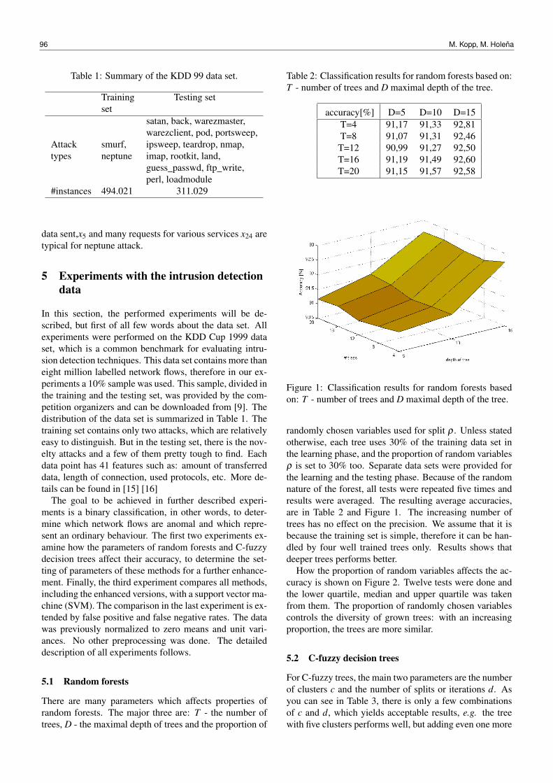
Table 1: Summary of the KDD 99 data set.

Trainingset

Testing set

satan, back, warezmaster,warezclient, pod, portsweep,

Attack smurf, ipsweep, teardrop, nmap,types neptune imap, rootkit, land,

guess_passwd, ftp_write,perl, loadmodule

#instances 494.021 311.029

data sent,x5 and many requests for various services x24 aretypical for neptune attack.

5 Experiments with the intrusion detectiondata

In this section, the performed experiments will be de-scribed, but first of all few words about the data set. Allexperiments were performed on the KDD Cup 1999 dataset, which is a common benchmark for evaluating intru-sion detection techniques. This data set contains more thaneight million labelled network flows, therefore in our ex-periments a 10% sample was used. This sample, divided inthe training and the testing set, was provided by the com-petition organizers and can be downloaded from [9]. Thedistribution of the data set is summarized in Table 1. Thetraining set contains only two attacks, which are relativelyeasy to distinguish. But in the testing set, there is the nov-elty attacks and a few of them pretty tough to find. Eachdata point has 41 features such as: amount of transferreddata, length of connection, used protocols, etc. More de-tails can be found in [15] [16]

The goal to be achieved in further described experi-ments is a binary classification, in other words, to deter-mine which network flows are anomal and which repre-sent an ordinary behaviour. The first two experiments ex-amine how the parameters of random forests and C-fuzzydecision trees affect their accuracy, to determine the set-ting of parameters of these methods for a further enhance-ment. Finally, the third experiment compares all methods,including the enhanced versions, with a support vector ma-chine (SVM). The comparison in the last experiment is ex-tended by false positive and false negative rates. The datawas previously normalized to zero means and unit vari-ances. No other preprocessing was done. The detaileddescription of all experiments follows.

5.1 Random forests

There are many parameters which affects properties ofrandom forests. The major three are: T - the number oftrees, D - the maximal depth of trees and the proportion of

Table 2: Classification results for random forests based on:T - number of trees and D maximal depth of the tree.

accuracy[%] D=5 D=10 D=15T=4 91,17 91,33 92,81T=8 91,07 91,31 92,46T=12 90,99 91,27 92,50T=16 91,19 91,49 92,60T=20 91,15 91,57 92,58

Figure 1: Classification results for random forests basedon: T - number of trees and D maximal depth of the tree.

randomly chosen variables used for split ρ . Unless statedotherwise, each tree uses 30% of the training data set inthe learning phase, and the proportion of random variablesρ is set to 30% too. Separate data sets were provided forthe learning and the testing phase. Because of the randomnature of the forest, all tests were repeated five times andresults were averaged. The resulting average accuracies,are in Table 2 and Figure 1. The increasing number oftrees has no effect on the precision. We assume that it isbecause the training set is simple, therefore it can be han-dled by four well trained trees only. Results shows thatdeeper trees performs better.

How the proportion of random variables affects the ac-curacy is shown on Figure 2. Twelve tests were done andthe lower quartile, median and upper quartile was takenfrom them. The proportion of randomly chosen variablescontrols the diversity of grown trees: with an increasingproportion, the trees are more similar.

5.2 C-fuzzy decision trees

For C-fuzzy trees, the main two parameters are the numberof clusters c and the number of splits or iterations d. Asyou can see in Table 3, there is only a few combinationsof c and d, which yields acceptable results, e.g. the treewith five clusters performs well, but adding even one more

96 M. Kopp, M. Holena

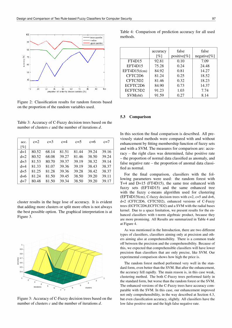
Figure 2: Classification results for random forests basedon the proportion of the random variables used.

Table 3: Accuracy of C-Fuzzy decision trees based on thenumber of clusters c and the number of iterations d.

acc. c=2 c=3 c=4 c=5 c=6 c=7[%]d=1 80.52 68.14 81.51 81.44 39.24 39.16d=2 80.52 68.08 39.27 81.46 38.50 39.24d=3 81.53 80.70 39.37 39.19 38.32 39.14d=4 81.33 81.07 39.36 39.19 38.43 38.37d=5 81.25 81.28 39.36 39.28 38.42 38.37d=6 81.24 81.50 39.45 38.50 39.20 39.11d=7 80.48 81.50 39.34 38.50 39.20 39.17

cluster results in the huge lose of accuracy. It is evidentthat adding more clusters or split more often is not alwaysthe best possible option. The graphical interpretation is atFigure 3.

23

45

67

12

34

56

7

0.4

0.5

0.6

0.7

0.8

0.9

1

clusters iterations

accu

racy

Figure 3: Accuracy of C-Fuzzy decision trees based on thenumber of clusters c and the number of iterations d.

Table 4: Comparison of prediction accuracy for all usedmethods.

accuracy false false[%] positive[%] negative[%]

FT4D15 92.81 0.10 7.09EFT4D15 75.28 0.24 24.48

EFT4D15(fcm) 84.92 0.81 14.27CFTC2D6 81.24 0.25 18.52CFTC5D2 81.46 0.32 18.23

ECFTC2D6 84.90 0.73 14.37ECFTC5D2 91.23 1.03 7.74

SVM(rbf) 91.59 0.27 8.14

5.3 Comparison

In this section the final comparison is described. All pre-viously stated methods were compared with and withoutenhancement by fitting membership function of fuzzy setsand with a SVM. The measures for comparison are: accu-racy – the right class was determined, false positive rate– the proportion of normal data classified as anomaly, andfalse negative rate – the proportion of anomal data classi-fied as normal.

For the final comparison, classifiers with the fol-lowing parameters were used: the random forest withT=4 and D=15 (FT4D15), the same tree enhanced withfuzzy sets (EFT4D15) and the same enhanced treewith the fuzzy c-means algorithm used for clustering(EFT4D15fcm), C-fuzzy decision trees with c=2, c=5 and d=6,d=2 (CFTC2D6, CFTC5D2), enhanced versions of C-Fuzzytrees (ECFTC2D6,ECFTC5D2) and a SVM with the radial baseskernel. Due to a space limitation, we present results for the en-hanced classifiers with t-norm algebraic product, because theyare more promising. All Results are summarized in Table 4 andat Figure 4.

As was mentioned in the Introduction, there are two differenttypes of classifiers, classifiers aiming only at precision and oth-ers aiming also at comprehensibility. There is a common tradeoff between the precision and the comprehensibility. Because ofthis, we expected that comprehensible classifiers will have lowerprecision than classifiers that are only precise, like SVM. Ourexperimental comparison shows how high the price is.

The random forest method performed very well in the stan-dard form, even better than the SVM. But after the enhancement,the accuracy fell rapidly. The main reason is, in this case weak,clustering method. The both C-Fuzzy trees performed fairly inthe standard form, but worse than the random forest or the SVM.The enhanced versions of the C-Fuzzy trees have accuracy com-parable with the SVM. In this case, our enhancement improvednot only comprehensibility, in the way described at Section 4.3,but even classification accuracy, slightly. All classifiers have thelow false positive rate and the high false negative rate.

Design and Comparison of Two Rule-based Fuzzy Classifiers for Computer Security 97

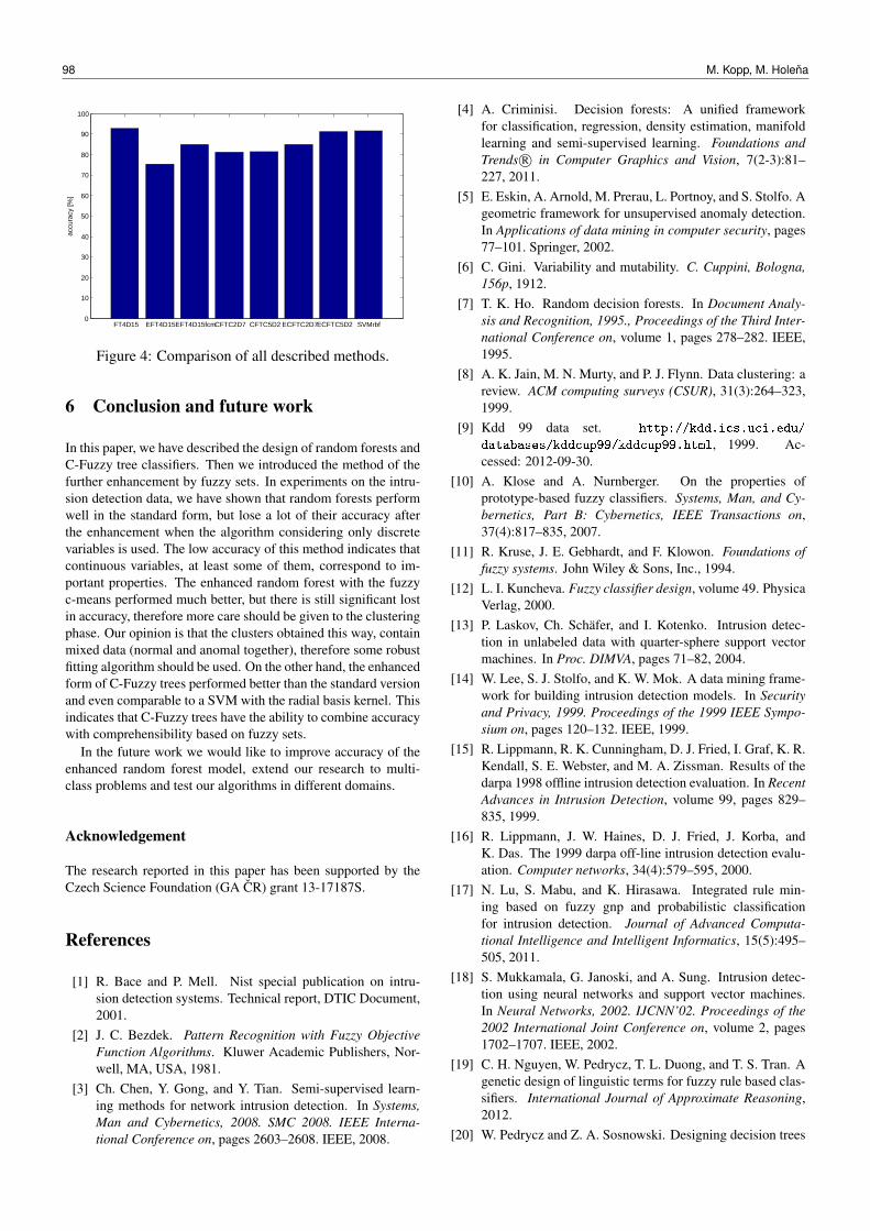
FT4D15 EFT4D15EFT4D15fcmCFTC2D7 CFTC5D2 ECFTC2D7ECFTC5D2 SVMrbf0

10

20

30

40

50

60

70

80

90

100

accu

racy

[%]

Figure 4: Comparison of all described methods.

6 Conclusion and future work

In this paper, we have described the design of random forests andC-Fuzzy tree classifiers. Then we introduced the method of thefurther enhancement by fuzzy sets. In experiments on the intru-sion detection data, we have shown that random forests performwell in the standard form, but lose a lot of their accuracy afterthe enhancement when the algorithm considering only discretevariables is used. The low accuracy of this method indicates thatcontinuous variables, at least some of them, correspond to im-portant properties. The enhanced random forest with the fuzzyc-means performed much better, but there is still significant lostin accuracy, therefore more care should be given to the clusteringphase. Our opinion is that the clusters obtained this way, containmixed data (normal and anomal together), therefore some robustfitting algorithm should be used. On the other hand, the enhancedform of C-Fuzzy trees performed better than the standard versionand even comparable to a SVM with the radial basis kernel. Thisindicates that C-Fuzzy trees have the ability to combine accuracywith comprehensibility based on fuzzy sets.

In the future work we would like to improve accuracy of theenhanced random forest model, extend our research to multi-class problems and test our algorithms in different domains.

Acknowledgement

The research reported in this paper has been supported by theCzech Science Foundation (GA CR) grant 13-17187S.

References

[1] R. Bace and P. Mell. Nist special publication on intru-sion detection systems. Technical report, DTIC Document,2001.

[2] J. C. Bezdek. Pattern Recognition with Fuzzy ObjectiveFunction Algorithms. Kluwer Academic Publishers, Nor-well, MA, USA, 1981.

[3] Ch. Chen, Y. Gong, and Y. Tian. Semi-supervised learn-ing methods for network intrusion detection. In Systems,Man and Cybernetics, 2008. SMC 2008. IEEE Interna-tional Conference on, pages 2603–2608. IEEE, 2008.

[4] A. Criminisi. Decision forests: A unified frameworkfor classification, regression, density estimation, manifoldlearning and semi-supervised learning. Foundations andTrends R© in Computer Graphics and Vision, 7(2-3):81–227, 2011.

[5] E. Eskin, A. Arnold, M. Prerau, L. Portnoy, and S. Stolfo. Ageometric framework for unsupervised anomaly detection.In Applications of data mining in computer security, pages77–101. Springer, 2002.

[6] C. Gini. Variability and mutability. C. Cuppini, Bologna,156p, 1912.

[7] T. K. Ho. Random decision forests. In Document Analy-sis and Recognition, 1995., Proceedings of the Third Inter-national Conference on, volume 1, pages 278–282. IEEE,1995.

[8] A. K. Jain, M. N. Murty, and P. J. Flynn. Data clustering: areview. ACM computing surveys (CSUR), 31(3):264–323,1999.

[9] Kdd 99 data set. http://kdd.ics.uci.edu/

databases/kddcup99/kddcup99.html, 1999. Ac-cessed: 2012-09-30.

[10] A. Klose and A. Nurnberger. On the properties ofprototype-based fuzzy classifiers. Systems, Man, and Cy-bernetics, Part B: Cybernetics, IEEE Transactions on,37(4):817–835, 2007.

[11] R. Kruse, J. E. Gebhardt, and F. Klowon. Foundations offuzzy systems. John Wiley & Sons, Inc., 1994.

[12] L. I. Kuncheva. Fuzzy classifier design, volume 49. PhysicaVerlag, 2000.

[13] P. Laskov, Ch. Schäfer, and I. Kotenko. Intrusion detec-tion in unlabeled data with quarter-sphere support vectormachines. In Proc. DIMVA, pages 71–82, 2004.

[14] W. Lee, S. J. Stolfo, and K. W. Mok. A data mining frame-work for building intrusion detection models. In Securityand Privacy, 1999. Proceedings of the 1999 IEEE Sympo-sium on, pages 120–132. IEEE, 1999.

[15] R. Lippmann, R. K. Cunningham, D. J. Fried, I. Graf, K. R.Kendall, S. E. Webster, and M. A. Zissman. Results of thedarpa 1998 offline intrusion detection evaluation. In RecentAdvances in Intrusion Detection, volume 99, pages 829–835, 1999.

[16] R. Lippmann, J. W. Haines, D. J. Fried, J. Korba, andK. Das. The 1999 darpa off-line intrusion detection evalu-ation. Computer networks, 34(4):579–595, 2000.

[17] N. Lu, S. Mabu, and K. Hirasawa. Integrated rule min-ing based on fuzzy gnp and probabilistic classificationfor intrusion detection. Journal of Advanced Computa-tional Intelligence and Intelligent Informatics, 15(5):495–505, 2011.

[18] S. Mukkamala, G. Janoski, and A. Sung. Intrusion detec-tion using neural networks and support vector machines.In Neural Networks, 2002. IJCNN’02. Proceedings of the2002 International Joint Conference on, volume 2, pages1702–1707. IEEE, 2002.

[19] C. H. Nguyen, W. Pedrycz, T. L. Duong, and T. S. Tran. Agenetic design of linguistic terms for fuzzy rule based clas-sifiers. International Journal of Approximate Reasoning,2012.

[20] W. Pedrycz and Z. A. Sosnowski. Designing decision trees

98 M. Kopp, M. Holena

with the use of fuzzy granulation. Systems, Man and Cy-bernetics, Part A: Systems and Humans, IEEE Transactionson, 30(2):151–159, 2000.

[21] W. Pedrycz and Z. A. Sosnowski. C-fuzzy decision trees.Systems, Man, and Cybernetics, Part C: Applications andReviews, IEEE Transactions on, 35(4):498–511, 2005.

[22] L. Portnoy, E. Eskin, and S. Stolfo. Intrusion detection withunlabeled data using clustering. In In Proceedings of ACMCSS Workshop on Data Mining Applied to Security (DMSA-2001. Citeseer, 2001.

[23] J. R. Quinlan. Induction of decision trees. Machine learn-ing, 1(1):81–106, 1986.

[24] J. R. Quinlan. C4. 5: programs for machine learning, vol-ume 1. Morgan kaufmann, 1993.

[25] G. Vigna and R. A. Kemmerer. Netstat: A network-basedintrusion detection approach. In Computer Security Appli-cations Conference, 1998. Proceedings. 14th Annual, pages25–34. IEEE, 1998.

Design and Comparison of Two Rule-based Fuzzy Classifiers for Computer Security 99

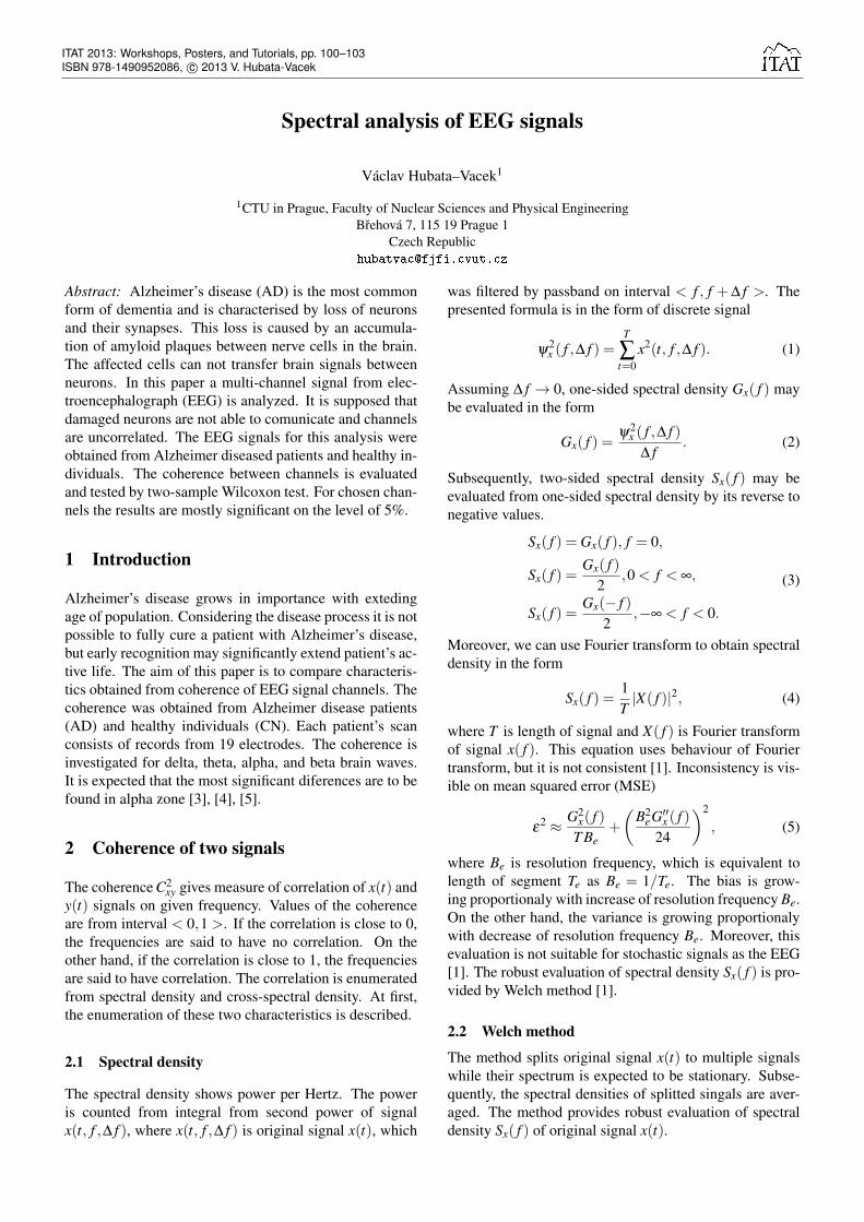
Spectral analysis of EEG signals

Václav Hubata–Vacek1

1CTU in Prague, Faculty of Nuclear Sciences and Physical EngineeringBrehová 7, 115 19 Prague 1

Czech Republichubatvac@fjfi.cvut.cz

Abstract: Alzheimer’s disease (AD) is the most commonform of dementia and is characterised by loss of neuronsand their synapses. This loss is caused by an accumula-tion of amyloid plaques between nerve cells in the brain.The affected cells can not transfer brain signals betweenneurons. In this paper a multi-channel signal from elec-troencephalograph (EEG) is analyzed. It is supposed thatdamaged neurons are not able to comunicate and channelsare uncorrelated. The EEG signals for this analysis wereobtained from Alzheimer diseased patients and healthy in-dividuals. The coherence between channels is evaluatedand tested by two-sample Wilcoxon test. For chosen chan-nels the results are mostly significant on the level of 5%.

1 Introduction

Alzheimer’s disease grows in importance with extedingage of population. Considering the disease process it is notpossible to fully cure a patient with Alzheimer’s disease,but early recognition may significantly extend patient’s ac-tive life. The aim of this paper is to compare characteris-tics obtained from coherence of EEG signal channels. Thecoherence was obtained from Alzheimer disease patients(AD) and healthy individuals (CN). Each patient’s scanconsists of records from 19 electrodes. The coherence isinvestigated for delta, theta, alpha, and beta brain waves.It is expected that the most significant diferences are to befound in alpha zone [3], [4], [5].

2 Coherence of two signals

The coherence C2xy gives measure of correlation of x(t) and

y(t) signals on given frequency. Values of the coherenceare from interval < 0,1 >. If the correlation is close to 0,the frequencies are said to have no correlation. On theother hand, if the correlation is close to 1, the frequenciesare said to have correlation. The correlation is enumeratedfrom spectral density and cross-spectral density. At first,the enumeration of these two characteristics is described.

2.1 Spectral density

The spectral density shows power per Hertz. The poweris counted from integral from second power of signalx(t, f ,∆ f ), where x(t, f ,∆ f ) is original signal x(t), which

was filtered by passband on interval < f , f +∆ f >. Thepresented formula is in the form of discrete signal

ψ2x ( f ,∆ f ) =

T

∑t=0

x2(t, f ,∆ f ). (1)

Assuming ∆ f → 0, one-sided spectral density Gx( f ) maybe evaluated in the form

Gx( f ) =ψ2

x ( f ,∆ f )∆ f

. (2)

Subsequently, two-sided spectral density Sx( f ) may beevaluated from one-sided spectral density by its reverse tonegative values.

Sx( f ) = Gx( f ), f = 0,

Sx( f ) =Gx( f )

2,0< f < ∞,

Sx( f ) =Gx(− f )

2,−∞< f < 0.

(3)

Moreover, we can use Fourier transform to obtain spectraldensity in the form

Sx( f ) =1T|X( f )|2, (4)

where T is length of signal and X( f ) is Fourier transformof signal x( f ). This equation uses behaviour of Fouriertransform, but it is not consistent [1]. Inconsistency is vis-ible on mean squared error (MSE)

ε2 ≈ G2x( f )

T Be+

(B2

eG′′x ( f )24

)2

, (5)

where Be is resolution frequency, which is equivalent tolength of segment Te as Be = 1/Te. The bias is grow-ing proportionaly with increase of resolution frequency Be.On the other hand, the variance is growing proportionalywith decrease of resolution frequency Be. Moreover, thisevaluation is not suitable for stochastic signals as the EEG[1]. The robust evaluation of spectral density Sx( f ) is pro-vided by Welch method [1].

2.2 Welch method

The method splits original signal x(t) to multiple signalswhile their spectrum is expected to be stationary. Subse-quently, the spectral densities of splitted singals are aver-aged. The method provides robust evaluation of spectraldensity Sx( f ) of original signal x(t).

ITAT 2013: Workshops, Posters, and Tutorials, pp. 100–103ISBN 978-1490952086, c© 2013 V. Hubata-Vacek

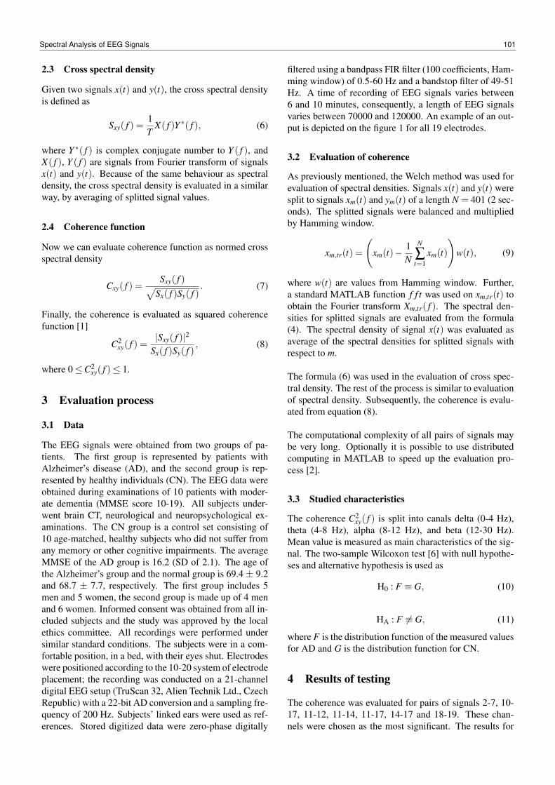
2.3 Cross spectral density

Given two signals x(t) and y(t), the cross spectral densityis defined as

Sxy( f ) =1T

X( f )Y ∗( f ), (6)

where Y ∗( f ) is complex conjugate number to Y ( f ), andX( f ), Y ( f ) are signals from Fourier transform of signalsx(t) and y(t). Because of the same behaviour as spectraldensity, the cross spectral density is evaluated in a similarway, by averaging of splitted signal values.

2.4 Coherence function

Now we can evaluate coherence function as normed crossspectral density

Cxy( f ) =Sxy( f )√

Sx( f )Sy( f ). (7)

Finally, the coherence is evaluated as squared coherencefunction [1]

C2xy( f ) =

|Sxy( f )|2Sx( f )Sy( f )

, (8)

where 0≤C2xy( f )≤ 1.

3 Evaluation process

3.1 Data

The EEG signals were obtained from two groups of pa-tients. The first group is represented by patients withAlzheimer’s disease (AD), and the second group is rep-resented by healthy individuals (CN). The EEG data wereobtained during examinations of 10 patients with moder-ate dementia (MMSE score 10-19). All subjects under-went brain CT, neurological and neuropsychological ex-aminations. The CN group is a control set consisting of10 age-matched, healthy subjects who did not suffer fromany memory or other cognitive impairments. The averageMMSE of the AD group is 16.2 (SD of 2.1). The age ofthe Alzheimer’s group and the normal group is 69.4 ± 9.2and 68.7 ± 7.7, respectively. The first group includes 5men and 5 women, the second group is made up of 4 menand 6 women. Informed consent was obtained from all in-cluded subjects and the study was approved by the localethics committee. All recordings were performed undersimilar standard conditions. The subjects were in a com-fortable position, in a bed, with their eyes shut. Electrodeswere positioned according to the 10-20 system of electrodeplacement; the recording was conducted on a 21-channeldigital EEG setup (TruScan 32, Alien Technik Ltd., CzechRepublic) with a 22-bit AD conversion and a sampling fre-quency of 200 Hz. Subjects’ linked ears were used as ref-erences. Stored digitized data were zero-phase digitally

filtered using a bandpass FIR filter (100 coefficients, Ham-ming window) of 0.5-60 Hz and a bandstop filter of 49-51Hz. A time of recording of EEG signals varies between6 and 10 minutes, consequently, a length of EEG signalsvaries between 70000 and 120000. An example of an out-put is depicted on the figure 1 for all 19 electrodes.

3.2 Evaluation of coherence

As previously mentioned, the Welch method was used forevaluation of spectral densities. Signals x(t) and y(t) weresplit to signals xm(t) and ym(t) of a length N = 401 (2 sec-onds). The splitted signals were balanced and multipliedby Hamming window.

xm,tr(t) =

(xm(t)−

1N

N

∑t=1

xm(t)

)w(t), (9)

where w(t) are values from Hamming window. Further,a standard MATLAB function f f t was used on xm,tr(t) toobtain the Fourier transform Xm,tr( f ). The spectral den-sities for splitted signals are evaluated from the formula(4). The spectral density of signal x(t) was evaluated asaverage of the spectral densities for splitted signals withrespect to m.

The formula (6) was used in the evaluation of cross spec-tral density. The rest of the process is similar to evaluationof spectral density. Subsequently, the coherence is evalu-ated from equation (8).

The computational complexity of all pairs of signals maybe very long. Optionally it is possible to use distributedcomputing in MATLAB to speed up the evaluation pro-cess [2].

3.3 Studied characteristics

The coherence C2xy( f ) is split into canals delta (0-4 Hz),

theta (4-8 Hz), alpha (8-12 Hz), and beta (12-30 Hz).Mean value is measured as main characteristics of the sig-nal. The two-sample Wilcoxon test [6] with null hypothe-ses and alternative hypothesis is used as

H0 : F ≡ G, (10)

HA : F 6≡ G, (11)

where F is the distribution function of the measured valuesfor AD and G is the distribution function for CN.

4 Results of testing

The coherence was evaluated for pairs of signals 2-7, 10-17, 11-12, 11-14, 11-17, 14-17 and 18-19. These chan-nels were chosen as the most significant. The results for

Spectral Analysis of EEG Signals 101

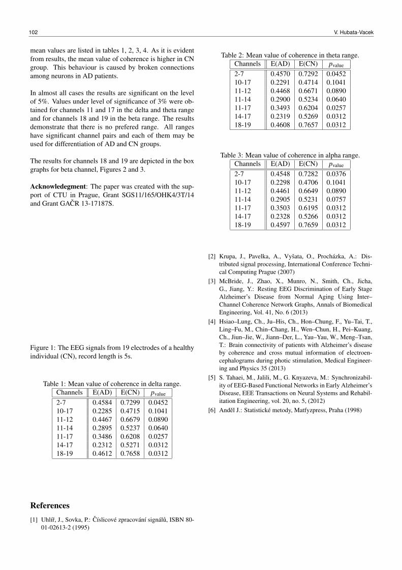
mean values are listed in tables 1, 2, 3, 4. As it is evidentfrom results, the mean value of coherence is higher in CNgroup. This behaviour is caused by broken connectionsamong neurons in AD patients.

In almost all cases the results are significant on the levelof 5%. Values under level of significance of 3% were ob-tained for channels 11 and 17 in the delta and theta rangeand for channels 18 and 19 in the beta range. The resultsdemonstrate that there is no prefered range. All rangeshave significant channel pairs and each of them may beused for differentiation of AD and CN groups.

The results for channels 18 and 19 are depicted in the boxgraphs for beta channel, Figures 2 and 3.

Acknowledegment: The paper was created with the sup-port of CTU in Prague, Grant SGS11/165/OHK4/3T/14and Grant GACR 13-17187S.

Figure 1: The EEG signals from 19 electrodes of a healthyindividual (CN), record length is 5s.

Table 1: Mean value of coherence in delta range.Channels E(AD) E(CN) pvalue

2-7 0.4584 0.7299 0.045210-17 0.2285 0.4715 0.104111-12 0.4467 0.6679 0.089011-14 0.2895 0.5237 0.064011-17 0.3486 0.6208 0.025714-17 0.2312 0.5271 0.031218-19 0.4612 0.7658 0.0312

References[1] Uhlír, J., Sovka, P.: Císlicové zpracování signálu, ISBN 80-

01-02613-2 (1995)

Table 2: Mean value of coherence in theta range.Channels E(AD) E(CN) pvalue

2-7 0.4570 0.7292 0.045210-17 0.2291 0.4714 0.104111-12 0.4468 0.6671 0.089011-14 0.2900 0.5234 0.064011-17 0.3493 0.6204 0.025714-17 0.2319 0.5269 0.031218-19 0.4608 0.7657 0.0312

Table 3: Mean value of coherence in alpha range.Channels E(AD) E(CN) pvalue

2-7 0.4548 0.7282 0.037610-17 0.2298 0.4706 0.104111-12 0.4461 0.6649 0.089011-14 0.2905 0.5231 0.075711-17 0.3503 0.6195 0.031214-17 0.2328 0.5266 0.031218-19 0.4597 0.7659 0.0312

[2] Krupa, J., Pavelka, A., Vyšata, O., Procházka, A.: Dis-tributed signal processing, International Conference Techni-cal Computing Prague (2007)

[3] McBride, J., Zhao, X., Munro, N., Smith, Ch., Jicha,G., Jiang, Y.: Resting EEG Discrimination of Early StageAlzheimer’s Disease from Normal Aging Using Inter–Channel Coherence Network Graphs, Annals of BiomedicalEngineering, Vol. 41, No. 6 (2013)

[4] Hsiao–Lung, Ch., Ju–His, Ch., Hon–Chung, F., Yu–Tai, T.,Ling–Fu, M., Chin–Chang, H., Wen–Chun, H., Pei–Kuang,Ch., Jiun–Jie, W., Jiann–Der, L., Yau–Yau, W., Meng–Tsan,T.: Brain connectivity of patients with Alzheimer’s diseaseby coherence and cross mutual information of electroen-cephalograms during photic stimulation, Medical Engineer-ing and Physics 35 (2013)

[5] S. Tahaei, M., Jalili, M., G. Knyazeva, M.: Synchronizabil-ity of EEG-Based Functional Networks in Early Alzheimer’sDisease, EEE Transactions on Neural Systems and Rehabil-itation Engineering, vol. 20, no. 5, (2012)

[6] Andel J.: Statistické metody, Matfyzpress, Praha (1998)

102 V. Hubata-Vacek

Table 4: Mean value of coherence in beta range.Channels E(AD) E(CN) pvalue

2-7 0.4687 0.7378 0.031210-17 0.2880 0.4980 0.104111-12 0.4907 0.6739 0.104111-14 0.3472 0.5505 0.075711-17 0.4084 0.6398 0.031214-17 0.2955 0.5532 0.031218-19 0.4941 0.7763 0.0257

Figure 2: Box graph of mean value for channels 18-19 inbeta range.

Figure 3: Box graph of standard deviation for channels18-19 in beta range.

Spectral Analysis of EEG Signals 103

Using machine learning methods in a personalized reputation system

Jirí Pejla1 and Martin Holena2

1 Faculty of Information Technology, Czech Technical University in PragueThákurova 9, 160 00 Praguejiri.pejla@gmail.com,

2 Institute of Computer Science, Academy of Sciences of the Czech RepublicPod Vodárenskou veží 2, 182 07 Prague

martin@cs.cas.cz

Abstract: Reputation systems become more and more im-portant in the on-line and e-commerce communities. Ex-ample widespread on-line system where reputation couldbe used is information system which allows users to rateeach other and express their experiences and opinions onsome products or services. In this paper, we are interestedin reputation of others from the perspective of one user.This reputation is called personalized and users can makeuse of it to find out proper information about certain prod-ucts. We implement personalized reputation system for in-formation systems using machine learning methods. Oursystem incorporates artificial neural networks and randomforests as well as a standard heuristic method, and it hasbeen tested on a large real world dataset.

1 Introduction

During their whole life, people must cooperate with oth-ers. Choosing friends and business partners has alwaysbeen based on the trust. One wants to cooperate only withpeople he trusts because he is not usually disappointed bythem. If we do not have enough own information and ex-periences with some person or company, we usually be-lieve other people’s opinions. On the opinion of majorityis based the notion of reputation.

These concepts are researched in many scientific fields,e.g. Economics, Psychology, Sociology etc. We focusonly on the field of Information Technology. In the In-ternet environment, it is very complicated to recognizewhether we should trust the other party, because for in-stance members are often anonymous and can enter andleave a community easily (see [6]). Thanks to the repu-tation systems, users can easily deduce their trust to un-known partners. That is why the reputation systems arevery important in the Internet communities.

There are many publications about theoretical aspects oftrust and reputation, e.g. paper [3] analysed the promisesand challenges of an online feedback mechanisms and pa-per [5] provided a survey of most known web trust and rep-utation systems and dealt with the problem of unfair rat-ings. This problem in the environment of e-marketplacesis solved in [8].

If one user has direct experience with another one, heeither trusts or distrusts him. This value of trust influ-ences the trust of his neighbours to the same user. This

process is called propagation of trust and it is used as theusual method for computing the reputation of particularuser (or generally, a node in a graph). A very comprehen-sive thesis on this topic is [6]. It deals with many compu-tational models of trust and reputation, with personaliza-tion and contextualization. There are also experiments oncentrality-based, preference-based and Bayesian estimateratings. Unfortunately, direct propagation of distrust is notinvolved in this thesis. Distrust is dealt in [4], and we usedformulas from this paper in our experiments.

Machine learning methods are not used very often forcomputation of trust. But if so, the results of experimentsshows that they are more effective and accurate. For in-stance [1] shows that support vector machines based repu-tation system better recognizes malicious nodes in the mis-sion critical networks. SVM and random forest algorithmscan be used in reputation systems for spam senders be-haviour analysis (see [7]). Artificial neural networks canbe also used for the implementation of reputation systems(see [9]). But their paper is aimed at broker-assisting sys-tems with subcommunities where agents do not have ac-cess to global information about history of transactions sothey have to gain information from other agents. It alsodeals with the personalized reputation and with the prob-lem of attacks.

To our knowledge, there are no publications about us-ing machine learning methods for computing personalizedreputation in general information systems where users canrate products or services and express their trust to otherusers. These information systems are very widespread andallow finding out relevant information and user experi-ence. In the paper, a computational model of reputationis built and the accuracy of two machine learning methodsis compared with the accuracy of one standard method ona real world dataset.

In the following section, the principles of used methodsand their parameters are recalled. Section 3 describes theused dataset and its statistics. The key section of the paperis Section 4 where we explain our approach and all impor-tant details of implementation. Results of experiments aresummarized in Section 5 and then concluded in Section 6.

ITAT 2013: Workshops, Posters, and Tutorials, pp. 104–110ISBN 978-1490952086, c© 2013 J. Pejla, M. Holena

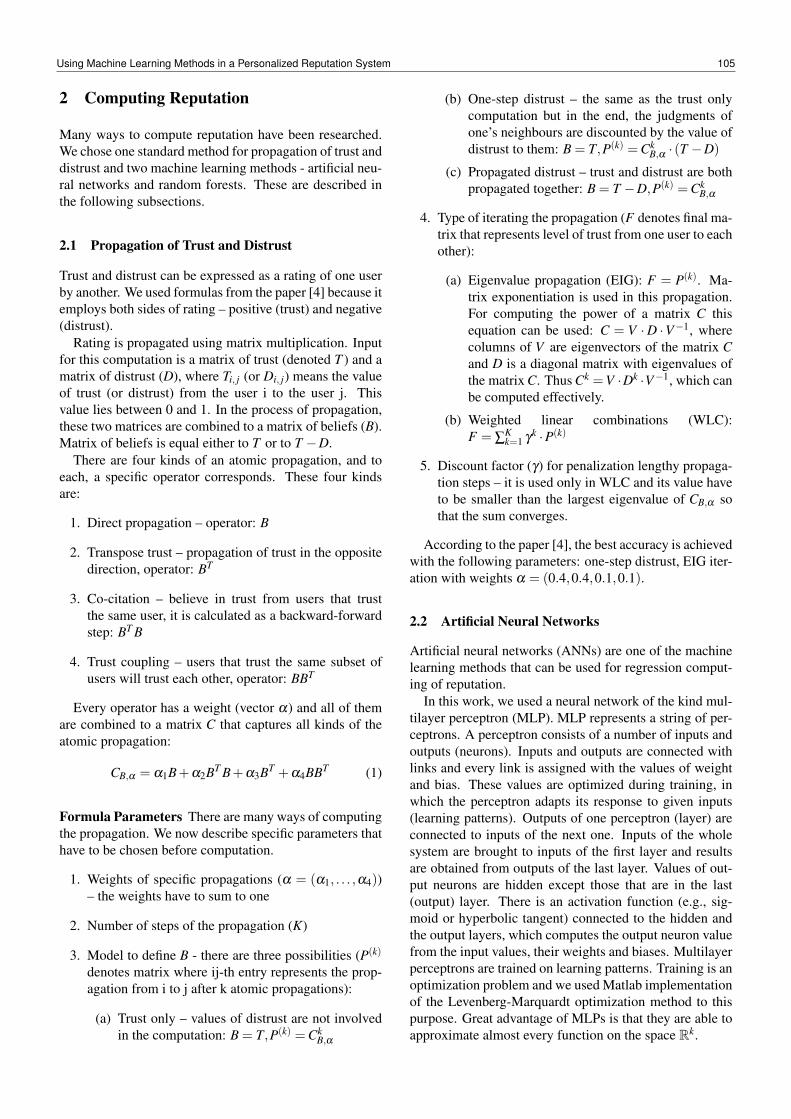
2 Computing Reputation

Many ways to compute reputation have been researched.We chose one standard method for propagation of trust anddistrust and two machine learning methods - artificial neu-ral networks and random forests. These are described inthe following subsections.

2.1 Propagation of Trust and Distrust

Trust and distrust can be expressed as a rating of one userby another. We used formulas from the paper [4] because itemploys both sides of rating – positive (trust) and negative(distrust).

Rating is propagated using matrix multiplication. Inputfor this computation is a matrix of trust (denoted T ) and amatrix of distrust (D), where Ti, j (or Di, j) means the valueof trust (or distrust) from the user i to the user j. Thisvalue lies between 0 and 1. In the process of propagation,these two matrices are combined to a matrix of beliefs (B).Matrix of beliefs is equal either to T or to T −D.

There are four kinds of an atomic propagation, and toeach, a specific operator corresponds. These four kindsare:

1. Direct propagation – operator: B

2. Transpose trust – propagation of trust in the oppositedirection, operator: BT

3. Co-citation – believe in trust from users that trustthe same user, it is calculated as a backward-forwardstep: BT B

4. Trust coupling – users that trust the same subset ofusers will trust each other, operator: BBT

Every operator has a weight (vector α) and all of themare combined to a matrix C that captures all kinds of theatomic propagation:

CB,α = α1B+α2BT B+α3BT +α4BBT (1)

Formula Parameters There are many ways of computingthe propagation. We now describe specific parameters thathave to be chosen before computation.

1. Weights of specific propagations (α = (α1, . . . ,α4))– the weights have to sum to one

2. Number of steps of the propagation (K)

3. Model to define B - there are three possibilities (P(k)

denotes matrix where ij-th entry represents the prop-agation from i to j after k atomic propagations):

(a) Trust only – values of distrust are not involvedin the computation: B = T,P(k) =Ck

B,α

(b) One-step distrust – the same as the trust onlycomputation but in the end, the judgments ofone’s neighbours are discounted by the value ofdistrust to them: B = T,P(k) =Ck

B,α · (T −D)

(c) Propagated distrust – trust and distrust are bothpropagated together: B = T −D,P(k) =Ck

B,α

4. Type of iterating the propagation (F denotes final ma-trix that represents level of trust from one user to eachother):

(a) Eigenvalue propagation (EIG): F = P(k). Ma-trix exponentiation is used in this propagation.For computing the power of a matrix C thisequation can be used: C = V ·D ·V−1, wherecolumns of V are eigenvectors of the matrix Cand D is a diagonal matrix with eigenvalues ofthe matrix C. Thus Ck =V ·Dk ·V−1, which canbe computed effectively.

(b) Weighted linear combinations (WLC):F = ∑K

k=1 γk ·P(k)

5. Discount factor (γ) for penalization lengthy propaga-tion steps – it is used only in WLC and its value haveto be smaller than the largest eigenvalue of CB,α sothat the sum converges.

According to the paper [4], the best accuracy is achievedwith the following parameters: one-step distrust, EIG iter-ation with weights α = (0.4,0.4,0.1,0.1).

2.2 Artificial Neural Networks

Artificial neural networks (ANNs) are one of the machinelearning methods that can be used for regression comput-ing of reputation.

In this work, we used a neural network of the kind mul-tilayer perceptron (MLP). MLP represents a string of per-ceptrons. A perceptron consists of a number of inputs andoutputs (neurons). Inputs and outputs are connected withlinks and every link is assigned with the values of weightand bias. These values are optimized during training, inwhich the perceptron adapts its response to given inputs(learning patterns). Outputs of one perceptron (layer) areconnected to inputs of the next one. Inputs of the wholesystem are brought to inputs of the first layer and resultsare obtained from outputs of the last layer. Values of out-put neurons are hidden except those that are in the last(output) layer. There is an activation function (e.g., sig-moid or hyperbolic tangent) connected to the hidden andthe output layers, which computes the output neuron valuefrom the input values, their weights and biases. Multilayerperceptrons are trained on learning patterns. Training is anoptimization problem and we used Matlab implementationof the Levenberg-Marquardt optimization method to thispurpose. Great advantage of MLPs is that they are able toapproximate almost every function on the space Rk.

Using Machine Learning Methods in a Personalized Reputation System 105

Parameters

1. Number of hidden layers

2. Number of hidden neurons

3. Activation function of hidden layers, and whether itis used also in the output layer

4. Training method

2.3 Random Forests

This subsection describes random regression forests and isbased on the paper [2].

A tree is an undirected graph without cycles. A deci-sion tree contains two types of nodes – split nodes (withtest function) and leaf nodes (with final answer). Input isinjected into the root node and according to the result oftest function in split nodes, it is sent to one of the childnodes until it arrives to the leaf node which contains theanswer.

Trees are tested by sending inputs to the root of a treeand collecting results from the leaf nodes that contain re-sults of regression. During training (an off-line phase),parameters of the split functions and the selection of finalanswers are optimized so as to minimize a chosen objec-tive function. The tree is growing until the given stoppingcriteria are met.

Random forest is an ensemble of trees that are trainedrandomly. It means that trees are trained on randomly dif-ferent subsets of input data or randomized node optimiza-tion is used. Individual trees have different depths and pa-rameters of the split nodes and this improves the general-ization capabilities of the resulting forest, because resultsare collected together from all trees. Forest training andtesting can be done in parallel which is very useful formodern computer architectures.

Components

1. Forest size – number of trees

2. Split functions – are characterized by a geometricprimitive that is used to separate the data, thresh-olds for tests, and a filter function that selects featuresfrom the input vector.

3. Objective function – with respect to this function, theparameters of a particular split node are optimizedduring the training phase (e.g., maximizing an infor-mation gain)

4. Randomness model – usually random training dataset sampling or randomized node optimization(makes available only a small random subset of pa-rameters of the split function).

5. Leaf prediction model – e.g., probabilistic predictoror point estimate

Table 1: Statistics of the input dataset

Statistic ValueNumber of users 9485Number of companies 2660Number of reviews 10030Number of ratings between users 10766Number of positive ratings between users 8199Number of negative ratings between users 2567

6. Ensemble model – how to combine results from alltrees, e.g., averaging

7. Stopping criteria – when to stop growing of the tree,e.g., maximum number of levels, minimum numberof training points in a node, etc.

3 Used Dataset

We used a real world dataset from the company TrustYard(information system on http://www.nejremeslnici.cz/). Onthis website, registered users can write reviews about ser-vices that were provided to them by some craft companiesor craftsmen. These reviews consist of textual descrip-tion and three grades – for quality of result, ratio of priceand service, and the behaviour to clients. Other users canrate this review with thumb up (positive rating) or down(negative rating). All these ratings are saved in the systemdatabase.

This dataset was anonymized (no names are included).Input data for the reputation system are split into two files– the first one contains reviews and the second one con-tains ratings of reviews. Basic statistics of the input datasetare introduced in Table 1. All inputs were split into twosubsets. One subset was used for training the machinelearning methods and searching for optimal parameters ofthe propagation of trust and distrust. The second subsetwas used for testing (comparing) all implemented meth-ods. The testing dataset contains entries from the last threemonths (approximately 15% of inputs), whereas the rest ofinputs is involved in training dataset. Number of the short-est paths between users in the testing and training datasetis displayed in Figure 3.

4 Proposed Design of a Reputation System

The aim of our work is to implement a personalized repu-tation system that provides for every user an ordered list ofother users according to their reputation from the point ofview of that user. This list is very useful - according to it,the system could offer to this user reviews of users that areclose to him or inherit the reputation of users to compa-nies they rated. The reviews of a user with higher reputa-tion would be more important. And all of these reputations

106 J. Pejla, M. Holena

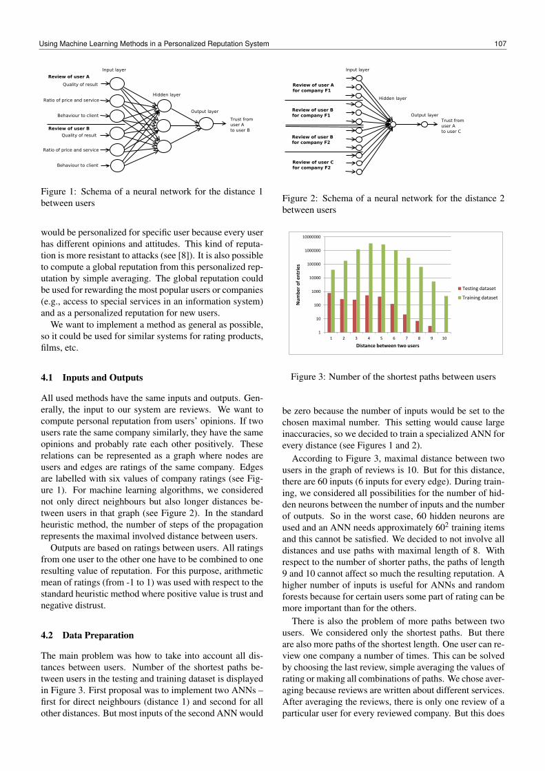
Input layer

Hidden layer

Output layer

Trust fromuser Ato user B

Review of user A

Review of user B

Quality of result

Ratio of price and service

Behaviour to client

Quality of result

Ratio of price and service

Behaviour to client

Figure 1: Schema of a neural network for the distance 1between users

would be personalized for specific user because every userhas different opinions and attitudes. This kind of reputa-tion is more resistant to attacks (see [8]). It is also possibleto compute a global reputation from this personalized rep-utation by simple averaging. The global reputation couldbe used for rewarding the most popular users or companies(e.g., access to special services in an information system)and as a personalized reputation for new users.

We want to implement a method as general as possible,so it could be used for similar systems for rating products,films, etc.

4.1 Inputs and Outputs

All used methods have the same inputs and outputs. Gen-erally, the input to our system are reviews. We want tocompute personal reputation from users’ opinions. If twousers rate the same company similarly, they have the sameopinions and probably rate each other positively. Theserelations can be represented as a graph where nodes areusers and edges are ratings of the same company. Edgesare labelled with six values of company ratings (see Fig-ure 1). For machine learning algorithms, we considerednot only direct neighbours but also longer distances be-tween users in that graph (see Figure 2). In the standardheuristic method, the number of steps of the propagationrepresents the maximal involved distance between users.

Outputs are based on ratings between users. All ratingsfrom one user to the other one have to be combined to oneresulting value of reputation. For this purpose, arithmeticmean of ratings (from -1 to 1) was used with respect to thestandard heuristic method where positive value is trust andnegative distrust.

4.2 Data Preparation

The main problem was how to take into account all dis-tances between users. Number of the shortest paths be-tween users in the testing and training dataset is displayedin Figure 3. First proposal was to implement two ANNs –first for direct neighbours (distance 1) and second for allother distances. But most inputs of the second ANN would

Review of user Afor company F1

Review of user Bfor company F2

Review of user Cfor company F2

Input layer

Hidden layer

Output layerTrust fromuser Ato user C

Review of user Bfor company F1

Figure 2: Schema of a neural network for the distance 2between users

1

10

100

1000

10000

100000

1000000

10000000

1 2 3 4 5 6 7 8 9 10

Nu

mb

er

of

en

trie

s

Distance between two users

Testing dataset

Training dataset

Figure 3: Number of the shortest paths between users

be zero because the number of inputs would be set to thechosen maximal number. This setting would cause largeinaccuracies, so we decided to train a specialized ANN forevery distance (see Figures 1 and 2).

According to Figure 3, maximal distance between twousers in the graph of reviews is 10. But for this distance,there are 60 inputs (6 inputs for every edge). During train-ing, we considered all possibilities for the number of hid-den neurons between the number of inputs and the numberof outputs. So in the worst case, 60 hidden neurons areused and an ANN needs approximately 602 training itemsand this cannot be satisfied. We decided to not involve alldistances and use paths with maximal length of 8. Withrespect to the number of shorter paths, the paths of length9 and 10 cannot affect so much the resulting reputation. Ahigher number of inputs is useful for ANNs and randomforests because for certain users some part of rating can bemore important than for the others.

There is also the problem of more paths between twousers. We considered only the shortest paths. But thereare also more paths of the shortest length. One user can re-view one company a number of times. This can be solvedby choosing the last review, simple averaging the values ofrating or making all combinations of paths. We chose aver-aging because reviews are written about different services.After averaging the reviews, there is only one review of aparticular user for every reviewed company. But this does

Using Machine Learning Methods in a Personalized Reputation System 107

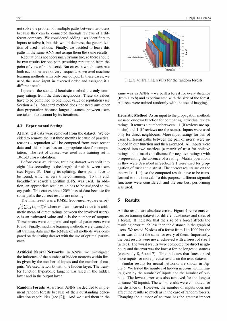
not solve the problem of multiple paths between two usersbecause they can be connected through reviews of a dif-ferent company. We considered adding user identifiers toinputs to solve it, but this would decrease the generaliza-tion of used methods. Finally, we decided to leave thispaths in the same ANN and assign them the same results.

Reputation is not necessarily symmetric, so there shouldbe two results for one path (resulting reputation from thepoint of view of both users). But cases in which users rateboth each other are not very frequent, so we used machinelearning methods with only one output. In these cases, weused the same input in reversed order and assigned it adifferent result.

Inputs to the standard heuristic method are only com-pany ratings from the direct neighbours. These six valueshave to be combined to one input value of reputation (seeSection 4.3). Standard method does not need any otherdata preparation because longer distances between usersare taken into account by its iterations.

4.3 Experimental Setting

At first, test data were removed from the dataset. We de-cided to remove the last three months because of practicalreasons – reputation will be computed from most recentdata and this subset has an appropriate size for compu-tation. The rest of dataset was used as a training set in10-fold cross-validation.

Before cross-validation, training dataset was split intoeight files according to the length of path between users(see Figure 3). During its splitting, these paths have tobe found, which is very time-consuming. To this end,breadth-first search algorithm (BFS) was used. In addi-tion, an appropriate result value has to be assigned to ev-ery path. This causes about 20% loss of data because forsome paths the correct results are missing.

The final result was a RMSE (root-mean-square error):√1n ∑n

i=1 (ei− ei)2 where ei is an observed value (the arith-metic mean of direct ratings between the involved users),ei is an estimated value and n is the number of outputs.These errors were compared and optimal parameters werefound. Finally, machine learning methods were trained onall training data and the RMSE of all methods was com-pared on the testing dataset with the use of optimal param-eters.

Artificial Neural Networks In ANNs, we investigatedthe influence of the number of hidden neurons within lim-its given by the number of inputs and the number of out-puts. We used networks with one hidden layer. The trans-fer function hyperbolic tangent was used in the hiddenlayer and in the output layer.

Random Forests Apart from ANNs we decided to imple-ment random forests because of their outstanding gener-alization capabilities (see [2]). And we used them in the

12345678

0

0.1

0.2

0.3

0.4

0.5

0.6

0.7

0.8

0.9

1

30

60

90

200

350

500

650

800950

Distance

RM

SE

Size of the forest

Figure 4: Training results for the random forests

same way as ANNs – we built a forest for every distance(from 1 to 8) and experimented with the size of the forest.All trees were trained randomly with the use of bagging.

Heuristic Method As an input to the propagation method,we used our own function for comparing individual reviewratings. It returns a number between−1 (if reviews are op-posite) and 1 (if reviews are the same). Inputs were usedonly for direct neighbours. More input ratings for pair ofusers (different paths between the pair of users) were in-cluded in our function and then averaged. All inputs wereinserted into two matrices (a matrix of trust for positiveratings and a matrix of distrust for negative ratings) with0 representing the absence of a rating. Matrix operationsas they were described in Section 2.1 were used for prop-agation of trust and distrust. The correct results are on theinterval 〈−1,1〉, so the computed results have to be trans-formed to this interval. To this purpose, different sigmoidfunctions were considered, and the one best performingwas used.

5 Results

All the results are absolute errors. Figure 4 represents er-rors on training dataset for different distances and sizes ofa forest. It indicates that the size of a forest affects theresulting error much less than the distance in the graph ofusers. We tested 29 sizes of a forest from 1 to 1000 but theerror was almost the same for every of them. Importantly,the best results were never achieved with a forest of size 1(a tree). The worst results were computed for direct neigh-bours and the error was the lowest for the longest distances(concretely 8, 6 and 7). This indicates that forests needmore inputs for more precise results on the used dataset.

Similar results for neural networks are shown in Fig-ure 5. We tested the number of hidden neurons within lim-its given by the number of inputs and the number of out-puts. The lowest error was also achieved for the longestdistance (48 inputs). The worst results were computed forthe distance 6. However, the number of inputs does notaffect the results so much as in the case of random forests.Changing the number of neurons has the greatest impact

108 J. Pejla, M. Holena

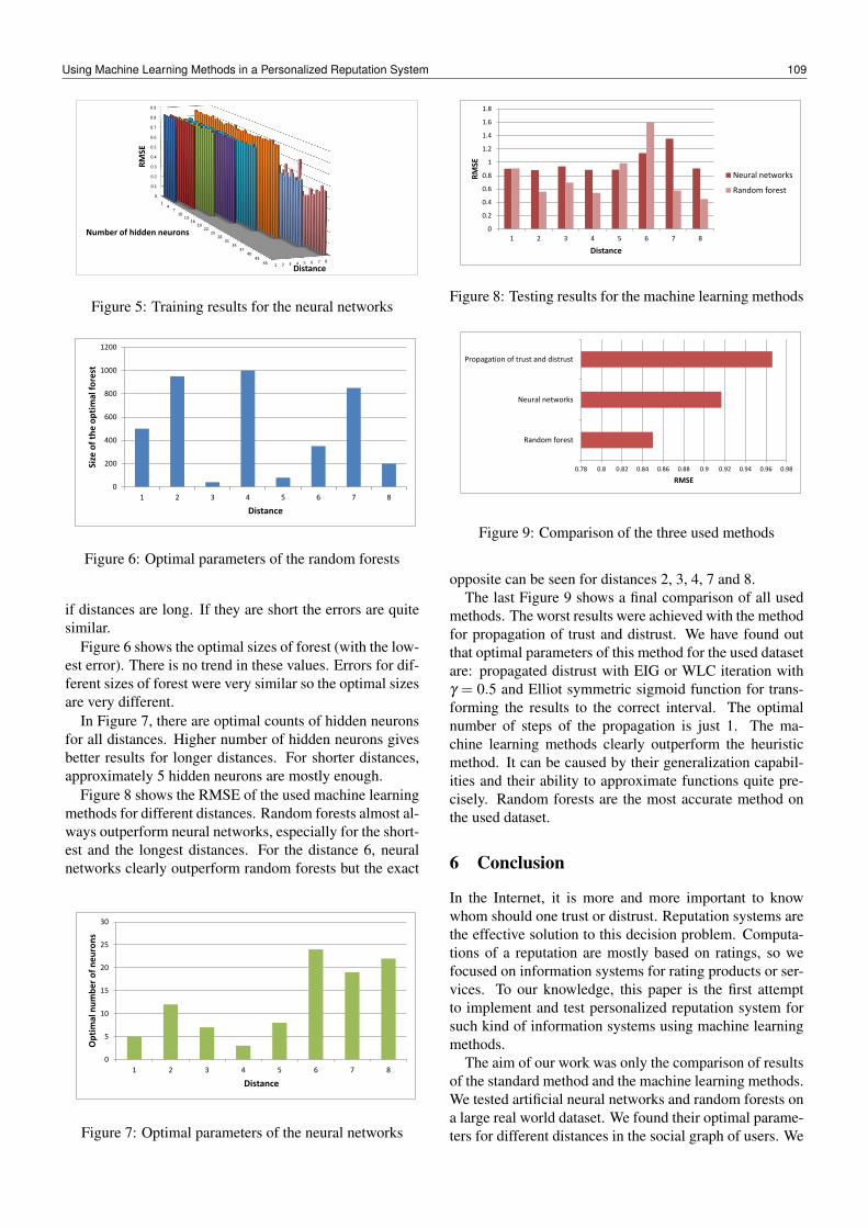
1 2 3 4 5 6 7 8

0

0.1

0.2

0.3

0.4

0.5

0.6

0.7

0.8

0.9

14

710

1316

1922

2528

3134

3740

4346

Distance

RM

SE

Number of hidden neurons

Figure 5: Training results for the neural networks

0

200

400

600

800

1000

1200

1 2 3 4 5 6 7 8

Size

of

the

op

tim

al f

ore

st

Distance

Figure 6: Optimal parameters of the random forests

if distances are long. If they are short the errors are quitesimilar.

Figure 6 shows the optimal sizes of forest (with the low-est error). There is no trend in these values. Errors for dif-ferent sizes of forest were very similar so the optimal sizesare very different.

In Figure 7, there are optimal counts of hidden neuronsfor all distances. Higher number of hidden neurons givesbetter results for longer distances. For shorter distances,approximately 5 hidden neurons are mostly enough.

Figure 8 shows the RMSE of the used machine learningmethods for different distances. Random forests almost al-ways outperform neural networks, especially for the short-est and the longest distances. For the distance 6, neuralnetworks clearly outperform random forests but the exact

0

5

10

15

20

25

30

1 2 3 4 5 6 7 8

Op

tim

al n

um

be

r o

f n

eu

ron

s

Distance

Figure 7: Optimal parameters of the neural networks

0

0.2

0.4

0.6

0.8

1

1.2

1.4

1.6

1.8

1 2 3 4 5 6 7 8

RM

SE

Distance

Neural networks

Random forest

Figure 8: Testing results for the machine learning methods

0.78 0.8 0.82 0.84 0.86 0.88 0.9 0.92 0.94 0.96 0.98

Random forest

Neural networks

Propagation of trust and distrust

RMSE

Figure 9: Comparison of the three used methods

opposite can be seen for distances 2, 3, 4, 7 and 8.The last Figure 9 shows a final comparison of all used

methods. The worst results were achieved with the methodfor propagation of trust and distrust. We have found outthat optimal parameters of this method for the used datasetare: propagated distrust with EIG or WLC iteration withγ = 0.5 and Elliot symmetric sigmoid function for trans-forming the results to the correct interval. The optimalnumber of steps of the propagation is just 1. The ma-chine learning methods clearly outperform the heuristicmethod. It can be caused by their generalization capabil-ities and their ability to approximate functions quite pre-cisely. Random forests are the most accurate method onthe used dataset.

6 Conclusion

In the Internet, it is more and more important to knowwhom should one trust or distrust. Reputation systems arethe effective solution to this decision problem. Computa-tions of a reputation are mostly based on ratings, so wefocused on information systems for rating products or ser-vices. To our knowledge, this paper is the first attemptto implement and test personalized reputation system forsuch kind of information systems using machine learningmethods.

The aim of our work was only the comparison of resultsof the standard method and the machine learning methods.We tested artificial neural networks and random forests ona large real world dataset. We found their optimal parame-ters for different distances in the social graph of users. We

Using Machine Learning Methods in a Personalized Reputation System 109

also experimented with different parameters of the stan-dard method for propagation of trust and distrust.

Machine learning methods are more and more used forcomputing a reputation, e.g., in the distributed networksor broker systems, and we have shown that they are appro-priate for computing a reputation also in the informationsystems for rating products and services. The most im-portant finding of the paper is that the machine learningmethods outperform the standard heuristic method on theused dataset.

Acknowledgement

The research reported in this paper has been supported bythe Czech Science Foundation (GA CR) grant 13-17187S.

References

[1] Akbani, R., Korkmaz, T. and Raju, G. V.: EMLTrust: Anenhanced Machine Learning based Reputation System forMANETs. Ad Hoc Netw. 10 (2012) 435–457,

[2] Criminisi, A., Shotton, J. and Konukoglu, E.: DecisionForests: A Unified Framework for Classification, Regres-sion, Density Estimation, Manifold Learning and Semi-Supervised Learning. Found. Trends. Comput. Graph. Vis.7 (2012) 81–227

[3] Dellarocas, Ch.: The Digitization of Word of Mouth:Promise and Challenges of Online Feedback Mechanisms.Manage. Sci. 60 (2003) 1407–1424

[4] Guha, R., Kumar, R., Raghavan, P. and Tomkins, A.: Prop-agation of trust and distrust. ACM WWW ’04 (2004) 403–412

[5] Jøsang, A., Ismail, R. and Boyd, C.: A survey of trust andreputation systems for online service provision. Decis. Sup-port Syst. 43 (2007) 618–644

[6] Mui, L.: Computational Models of Trust and Reputation:Agents, Evolutionary Games, and Social Networks. PhDThesis, MIT (2002)

[7] Tang, Y., Krasser, S. He, Y., Yang, W. Alperovitch, D.:Support Vector Machines and Random Forests Modelingfor Spam Senders Behavior Analysis. IEEE GLOBECOM(2008) 2174-2178

[8] Zhang, J., Cohen, R.: Trusting advice from other buyers ine-marketplaces: the problem of unfair ratings ACM ICEC’06 (2006) 225–234

[9] Zong, B., Xu, F., Jiao, J. and Lü, J.: A Broker-Assisting Trustand Reputation System Based on Artificial Neural Network.IEEE SMC (2009) 4710–4715

110 J. Pejla, M. Holena

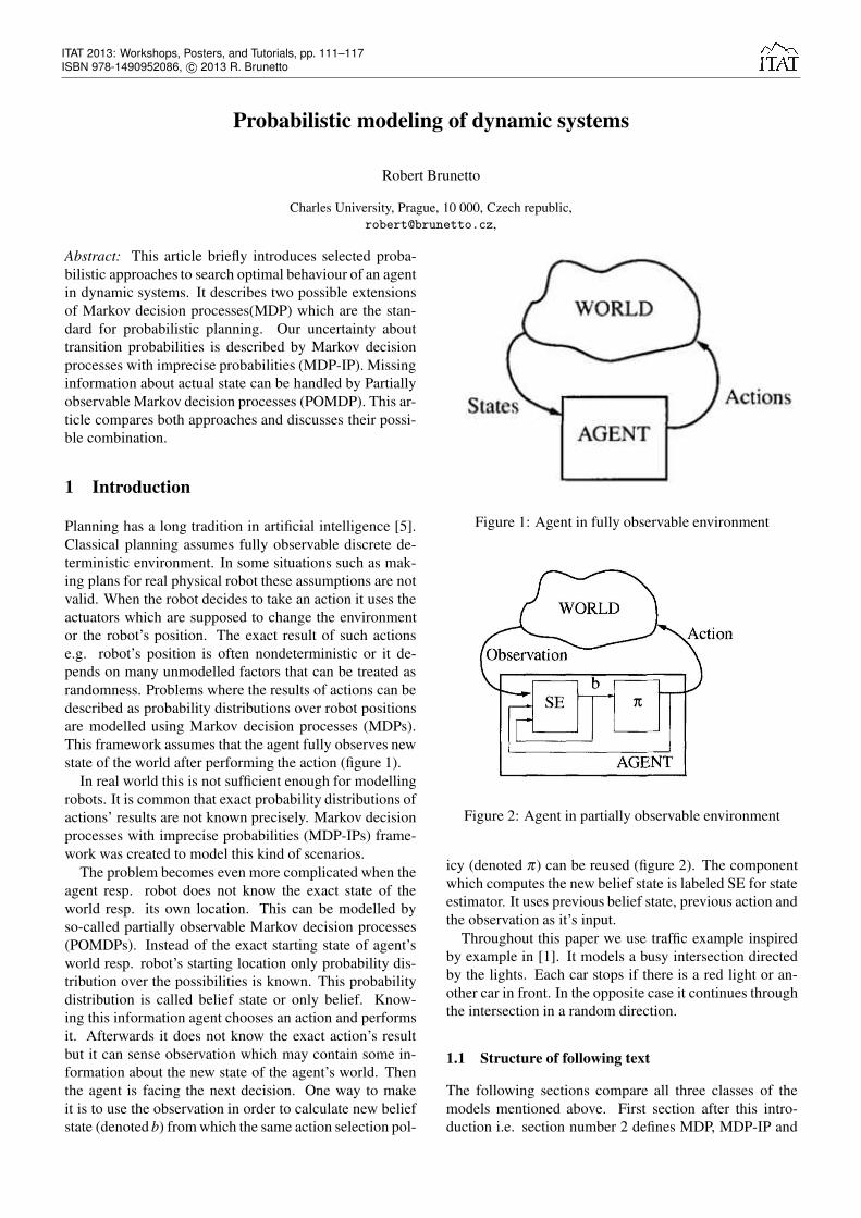
Probabilistic modeling of dynamic systems

Robert Brunetto

Charles University, Prague, 10 000, Czech republic,robert@brunetto.cz,

Abstract: This article briefly introduces selected proba-bilistic approaches to search optimal behaviour of an agentin dynamic systems. It describes two possible extensionsof Markov decision processes(MDP) which are the stan-dard for probabilistic planning. Our uncertainty abouttransition probabilities is described by Markov decisionprocesses with imprecise probabilities (MDP-IP). Missinginformation about actual state can be handled by Partiallyobservable Markov decision processes (POMDP). This ar-ticle compares both approaches and discusses their possi-ble combination.

1 Introduction

Planning has a long tradition in artificial intelligence [5].Classical planning assumes fully observable discrete de-terministic environment. In some situations such as mak-ing plans for real physical robot these assumptions are notvalid. When the robot decides to take an action it uses theactuators which are supposed to change the environmentor the robot’s position. The exact result of such actionse.g. robot’s position is often nondeterministic or it de-pends on many unmodelled factors that can be treated asrandomness. Problems where the results of actions can bedescribed as probability distributions over robot positionsare modelled using Markov decision processes (MDPs).This framework assumes that the agent fully observes newstate of the world after performing the action (figure 1).

In real world this is not sufficient enough for modellingrobots. It is common that exact probability distributions ofactions’ results are not known precisely. Markov decisionprocesses with imprecise probabilities (MDP-IPs) frame-work was created to model this kind of scenarios.

The problem becomes even more complicated when theagent resp. robot does not know the exact state of theworld resp. its own location. This can be modelled byso-called partially observable Markov decision processes(POMDPs). Instead of the exact starting state of agent’sworld resp. robot’s starting location only probability dis-tribution over the possibilities is known. This probabilitydistribution is called belief state or only belief. Know-ing this information agent chooses an action and performsit. Afterwards it does not know the exact action’s resultbut it can sense observation which may contain some in-formation about the new state of the agent’s world. Thenthe agent is facing the next decision. One way to makeit is to use the observation in order to calculate new beliefstate (denoted b) from which the same action selection pol-

Figure 1: Agent in fully observable environment

Figure 2: Agent in partially observable environment

icy (denoted π) can be reused (figure 2). The componentwhich computes the new belief state is labeled SE for stateestimator. It uses previous belief state, previous action andthe observation as it’s input.

Throughout this paper we use traffic example inspiredby example in [1]. It models a busy intersection directedby the lights. Each car stops if there is a red light or an-other car in front. In the opposite case it continues throughthe intersection in a random direction.

1.1 Structure of following text

The following sections compare all three classes of themodels mentioned above. First section after this intro-duction i.e. section number 2 defines MDP, MDP-IP and

ITAT 2013: Workshops, Posters, and Tutorials, pp. 111–117ISBN 978-1490952086, c© 2013 R. Brunetto

POMDP formally and shows their differences on the traf-fic example. The next section defines policy for both fullyand partially observable environments which allows us todefine optimal policy for all three classes of models. Com-puting optimal policy is our goal. The way to achieve itis similar for all three classes of models. This article ex-plains it and compares the calculations needed for solvingall three classes of models also in section 3. The contribu-tion of this article is the discussion of possible combina-tion of all three model types. It can be found in the section4.

2 Definitions

This section formally defines MDPs, POMDPs and MDP-IPs and shows their possible usage on examples.

2.1 Markov Decision processes (MDPs)

MDPs are defined as tuples of the form (S,A,R,T ) where

• S is a set of states

• A is a set of actions

• R is a reward function S×A → R telling how muchthe agent is rewarded for taking a given action in agiven state.

• T is a transition function S×A×S → [0,1] giving theprobability T (st ,at ,st+1) of moving from state st tostate st+1 by executing action at .

In our example the set of states encodes positions of all thecars. The set of actions contains possible light combina-tions. Transition function would describe car movementsand their probabilities. The reward function would be setup the way to minimize number of cars waiting at the in-tersection.

MDPs are standard framework for planning under un-certainty in fully obserable environments with known tran-sition probabilities.

2.2 Partially observable Markov decision processes(POMDPs)

One of the reasons why modelling intersection with MDPis unrealistic is that it is not common that the sensors atthe intersection could know the precise location of all cars.More typically only partial information about positions ofsome cars at the intersection is observed. The probabilitiesof receiving possible observations are defined by observa-tion function.

POMDPs are defined as tuples of the form(S,A,R,T,Ω,O) where

• S, A, R and T are the same as in the MDP.

• Ω is a set of observations

• O : S×A×Ω → [0,1] is the observation function giv-ing the probability of observations for given statesand actions.

The difference of POMDP agent from MDP agent is thefact that the POMDP agent can not observe the state. In-stead of that it only receives observation o which is ran-domly drawn from Ω according to probablitities given byobservation function.

2.3 Markov decision processes with imprecisetransition probabilities (MDP-IPs)

Another reason why modelling intersection using MDP isunrealistic is that we usually do not know the exact prob-abilities of cars’ behaviour. It depends on the time, onthe day of week, on holidays, on regional events and onother factors. Instead of searching optimal intersection be-haviour for one setup of probabilities one would rather findpolicy always behaving reasonably. MDP-IPs can be uti-lized to find it. MDP-IPs are defined as tuples of the form(S,A,R,K) where

• S, A and R are defined the same way as in MDPs.

• K is a set of transition functions, K ⊆ T |T : S×A×S → [0,1], i.e. set of functions which prescribesthe probabilities of resulting states after performinggiven action from given previous state.

Delgado et al. [1] shown how to solve MDP-IPs effec-tively under some conditions. They assumed that K is ei-ther finite or can be expressed by finite set of linear con-strains.

MDP-IPs are used in cases when the environment isfully observable but the transition function is not knownprecisely. In contrast to MDP the transition function is re-placed by the set of possible transition functions in MDP-IPs case.

MDPs are special cases of MDP-IPs where K = T.

2.4 Common background

In the beginning the agent is in the state s0. The MDP andMDP-IP frameworks assume that this state is known bythe agent. The POMDP framework assume that the agentknows the probability distribution b0 of initial states.

At each time period t the agent chooses action at ∈ Aaccordingly to state st resp. belief state bt . Perfomingthis action causes the state random change to st+1. Theprobabilities of transitions are given by transition functionT , P(st+1|st ,at) = T (st ,at ,st+1).

The agent receives a reward rt according to reward func-tion, rt = R(st+1,at). Note that this reward is not observedby the agent in partially observable case. The only infor-mation agent has in partially observable case is observa-tion ot which is randomly drawn from the set of observa-tions O with respect to probabilities given by observationfunction O, P(ot |st+1,at) = O(st+1,at ,ot ).

112 R. Brunetto

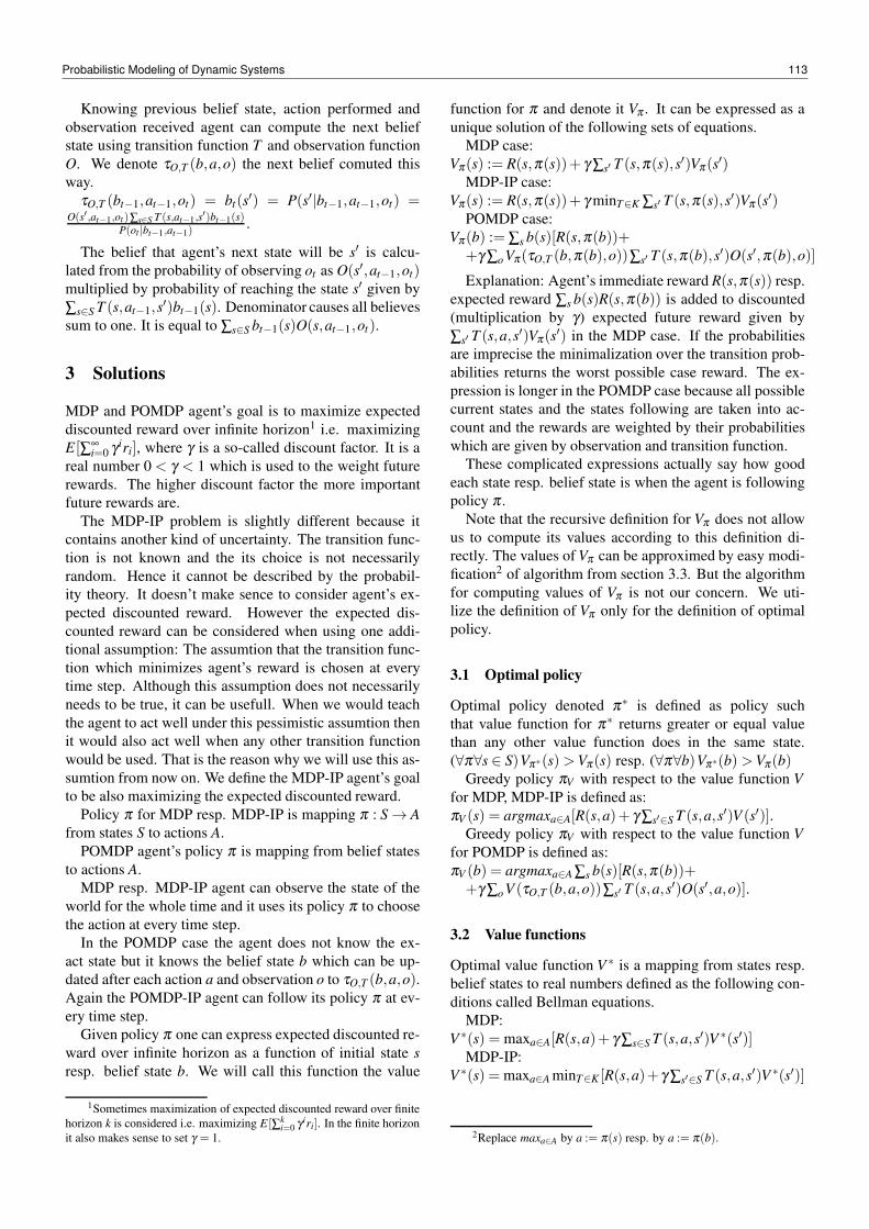
Knowing previous belief state, action performed andobservation received agent can compute the next beliefstate using transition function T and observation functionO. We denote τO,T (b,a,o) the next belief comuted thisway.

τO,T (bt−1,at−1,ot) = bt(s′) = P(s′|bt−1,at−1,ot) =O(s′,at−1,ot )∑s∈S T (s,at−1,s′)bt−1(s)

P(ot |bt−1,at−1).

The belief that agent’s next state will be s′ is calcu-lated from the probability of observing ot as O(s′,at−1,ot)multiplied by probability of reaching the state s′ given by∑s∈S T (s,at−1,s′)bt−1(s). Denominator causes all believessum to one. It is equal to ∑s∈S bt−1(s)O(s,at−1,ot).

3 Solutions

MDP and POMDP agent’s goal is to maximize expecteddiscounted reward over infinite horizon1 i.e. maximizingE[∑∞

i=0 γ iri], where γ is a so-called discount factor. It is areal number 0 < γ < 1 which is used to the weight futurerewards. The higher discount factor the more importantfuture rewards are.

The MDP-IP problem is slightly different because itcontains another kind of uncertainty. The transition func-tion is not known and the its choice is not necessarilyrandom. Hence it cannot be described by the probabil-ity theory. It doesn’t make sence to consider agent’s ex-pected discounted reward. However the expected dis-counted reward can be considered when using one addi-tional assumption: The assumtion that the transition func-tion which minimizes agent’s reward is chosen at everytime step. Although this assumption does not necessarilyneeds to be true, it can be usefull. When we would teachthe agent to act well under this pessimistic assumtion thenit would also act well when any other transition functionwould be used. That is the reason why we will use this as-sumtion from now on. We define the MDP-IP agent’s goalto be also maximizing the expected discounted reward.

Policy π for MDP resp. MDP-IP is mapping π : S → Afrom states S to actions A.

POMDP agent’s policy π is mapping from belief statesto actions A.

MDP resp. MDP-IP agent can observe the state of theworld for the whole time and it uses its policy π to choosethe action at every time step.

In the POMDP case the agent does not know the ex-act state but it knows the belief state b which can be up-dated after each action a and observation o to τO,T (b,a,o).Again the POMDP-IP agent can follow its policy π at ev-ery time step.

Given policy π one can express expected discounted re-ward over infinite horizon as a function of initial state sresp. belief state b. We will call this function the value

1Sometimes maximization of expected discounted reward over finitehorizon k is considered i.e. maximizing E[∑k

i=0 γ iri]. In the finite horizonit also makes sense to set γ = 1.

function for π and denote it Vπ . It can be expressed as aunique solution of the following sets of equations.

MDP case:Vπ(s) := R(s,π(s))+ γ ∑s′ T (s,π(s),s′)Vπ(s′)

MDP-IP case:Vπ(s) := R(s,π(s))+ γ minT∈K ∑s′ T (s,π(s),s′)Vπ(s′)

POMDP case:Vπ(b) := ∑s b(s)[R(s,π(b))+

+γ ∑o Vπ(τO,T (b,π(b),o))∑s′ T (s,π(b),s′)O(s′,π(b),o)]Explanation: Agent’s immediate reward R(s,π(s)) resp.

expected reward ∑s b(s)R(s,π(b)) is added to discounted(multiplication by γ) expected future reward given by∑s′ T (s,a,s′)Vπ(s′) in the MDP case. If the probabilitiesare imprecise the minimalization over the transition prob-abilities returns the worst possible case reward. The ex-pression is longer in the POMDP case because all possiblecurrent states and the states following are taken into ac-count and the rewards are weighted by their probabilitieswhich are given by observation and transition function.

These complicated expressions actually say how goodeach state resp. belief state is when the agent is followingpolicy π .

Note that the recursive definition for Vπ does not allowus to compute its values according to this definition di-rectly. The values of Vπ can be approximed by easy modi-fication2 of algorithm from section 3.3. But the algorithmfor computing values of Vπ is not our concern. We uti-lize the definition of Vπ only for the definition of optimalpolicy.

3.1 Optimal policy

Optimal policy denoted π∗ is defined as policy suchthat value function for π∗ returns greater or equal valuethan any other value function does in the same state.(∀π∀s ∈ S)Vπ∗(s)>Vπ(s) resp. (∀π∀b)Vπ∗(b)>Vπ(b)

Greedy policy πV with respect to the value function Vfor MDP, MDP-IP is defined as:πV (s) = argmaxa∈A[R(s,a)+ γ ∑s′∈S T (s,a,s′)V (s′)].

Greedy policy πV with respect to the value function Vfor POMDP is defined as:πV (b) = argmaxa∈A ∑s b(s)[R(s,π(b))++γ ∑o V (τO,T (b,a,o))∑s′ T (s,a,s′)O(s′,a,o)].

3.2 Value functions

Optimal value function V ∗ is a mapping from states resp.belief states to real numbers defined as the following con-ditions called Bellman equations.

MDP:V ∗(s) = maxa∈A[R(s,a)+ γ ∑s∈S T (s,a,s′)V ∗(s′)]

MDP-IP:V ∗(s) = maxa∈A minT∈K [R(s,a)+ γ ∑s′∈S T (s,a,s′)V ∗(s′)]

2Replace maxa∈A by a := π(s) resp. by a := π(b).

Probabilistic Modeling of Dynamic Systems 113

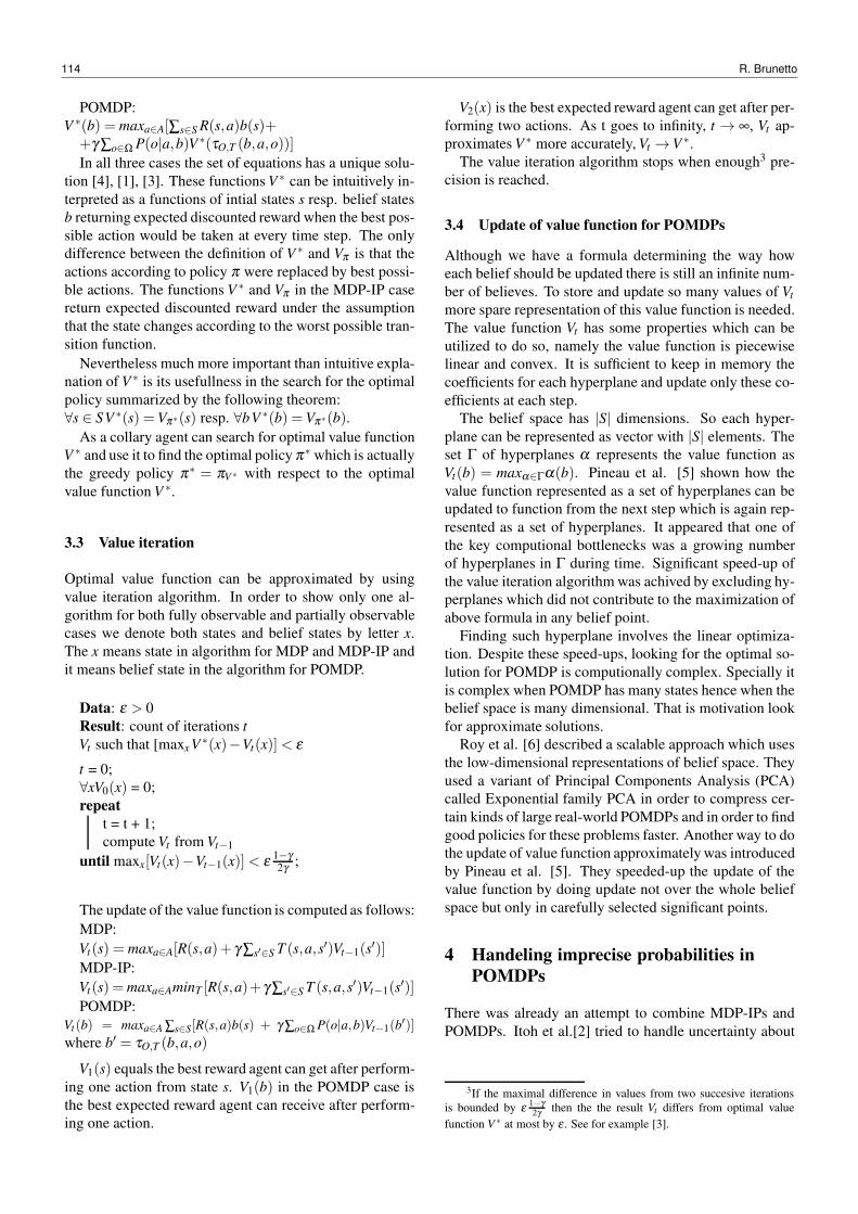
POMDP:V ∗(b) = maxa∈A[∑s∈S R(s,a)b(s)+

+γ ∑o∈Ω P(o|a,b)V ∗(τO,T (b,a,o))]In all three cases the set of equations has a unique solu-

tion [4], [1], [3]. These functions V ∗ can be intuitively in-terpreted as a functions of intial states s resp. belief statesb returning expected discounted reward when the best pos-sible action would be taken at every time step. The onlydifference between the definition of V ∗ and Vπ is that theactions according to policy π were replaced by best possi-ble actions. The functions V ∗ and Vπ in the MDP-IP casereturn expected discounted reward under the assumptionthat the state changes according to the worst possible tran-sition function.

Nevertheless much more important than intuitive expla-nation of V ∗ is its usefullness in the search for the optimalpolicy summarized by the following theorem:∀s ∈ SV ∗(s) =Vπ∗(s) resp. ∀bV ∗(b) =Vπ∗(b).

As a collary agent can search for optimal value functionV ∗ and use it to find the optimal policy π∗ which is actuallythe greedy policy π∗ = πV∗ with respect to the optimalvalue function V ∗.

3.3 Value iteration

Optimal value function can be approximated by usingvalue iteration algorithm. In order to show only one al-gorithm for both fully observable and partially observablecases we denote both states and belief states by letter x.The x means state in algorithm for MDP and MDP-IP andit means belief state in the algorithm for POMDP.

Data: ε > 0Result: count of iterations tVt such that [maxx V ∗(x)−Vt(x)]< εt = 0;∀xV0(x) = 0;repeat

t = t + 1;compute Vt from Vt−1

until maxx[Vt(x)−Vt−1(x)]< ε 1−γ2γ ;

The update of the value function is computed as follows:MDP:Vt(s) = maxa∈A[R(s,a)+ γ ∑s′∈S T (s,a,s′)Vt−1(s′)]MDP-IP:Vt(s) =maxa∈AminT [R(s,a)+γ ∑s′∈S T (s,a,s′)Vt−1(s′)]POMDP:

Vt(b) = maxa∈A ∑s∈S[R(s,a)b(s) + γ ∑o∈Ω P(o|a,b)Vt−1(b′)]where b′ = τO,T (b,a,o)

V1(s) equals the best reward agent can get after perform-ing one action from state s. V1(b) in the POMDP case isthe best expected reward agent can receive after perform-ing one action.

V2(x) is the best expected reward agent can get after per-forming two actions. As t goes to infinity, t → ∞, Vt ap-proximates V ∗ more accurately, Vt →V ∗.

The value iteration algorithm stops when enough3 pre-cision is reached.

3.4 Update of value function for POMDPs

Although we have a formula determining the way howeach belief should be updated there is still an infinite num-ber of believes. To store and update so many values of Vtmore spare representation of this value function is needed.The value function Vt has some properties which can beutilized to do so, namely the value function is piecewiselinear and convex. It is sufficient to keep in memory thecoefficients for each hyperplane and update only these co-efficients at each step.

The belief space has |S| dimensions. So each hyper-plane can be represented as vector with |S| elements. Theset Γ of hyperplanes α represents the value function asVt(b) = maxα∈Γα(b). Pineau et al. [5] shown how thevalue function represented as a set of hyperplanes can beupdated to function from the next step which is again rep-resented as a set of hyperplanes. It appeared that one ofthe key computional bottlenecks was a growing numberof hyperplanes in Γ during time. Significant speed-up ofthe value iteration algorithm was achived by excluding hy-perplanes which did not contribute to the maximization ofabove formula in any belief point.

Finding such hyperplane involves the linear optimiza-tion. Despite these speed-ups, looking for the optimal so-lution for POMDP is computionally complex. Specially itis complex when POMDP has many states hence when thebelief space is many dimensional. That is motivation lookfor approximate solutions.

Roy et al. [6] described a scalable approach which usesthe low-dimensional representations of belief space. Theyused a variant of Principal Components Analysis (PCA)called Exponential family PCA in order to compress cer-tain kinds of large real-world POMDPs and in order to findgood policies for these problems faster. Another way to dothe update of value function approximately was introducedby Pineau et al. [5]. They speeded-up the update of thevalue function by doing update not over the whole beliefspace but only in carefully selected significant points.

4 Handeling imprecise probabilities inPOMDPs

There was already an attempt to combine MDP-IPs andPOMDPs. Itoh et al.[2] tried to handle uncertainty about

3If the maximal difference in values from two succesive iterationsis bounded by ε 1−γ

2γ then the the result Vt differs from optimal valuefunction V ∗ at most by ε . See for example [3].

114 R. Brunetto

transtion and observation models by defining partially ob-servable Markov decision processes with imprecise prob-abilities (POMDPIPs).

They searched for the solution of problems in two fol-lowing cases: 1. when the sets of possible models formpolytopes, 2. when the sets of possible models are finite.They shown how to solve this kind of problems effectivelybut they used quite different definition of optimal solutionthan we did. They used so-called second order believes todefine probabilities over spaces of transition and observa-tion models. Itoh et al. [2] defined POMDPIP’s policy asoptimal whenever the optimal policy existed for any sec-ond order belief.

This definition of optimal policy is unintuitional. Recallour transportation example. The transition models dependon holidays, regional events and other unmodelled factors.This uncertainty is encoded as a set of possible transitionmodels. Similarily the observability can be different dur-ing the day and night.

According to definition of Itoh et al. [2] we can think ofany second order belief e.g. belief such that the probabilityof the night observation model is 95% and the probabilityof the day observation model is 5% and then if we foundoptimal policy for this second order belief we would callit the optimal policy for the whole POMDPIP.

In many cases as in the traffic example one would liketo find the policy which performs well for all (or at leastfor most) possible transition and observation models ratherthan the strategy performing well only for some specificcombination of these models.

Good choice of the action to take would be the actionmaximizing expected value for the worst possible choiceof transition and observation model i.e. action accordingto policy πV∗ where

V ∗(b) = maxa∈AminT minO ∑s∈S

[R(s,a)b(s)+

+γ ∑o∈Ω

P(o|a,b)V ∗(τO,T (b,a,o))]

Another possibility of overcoming imprecision of prob-abilities is taking expectation over all possible observationand transition models4.

V ∗(b) = maxa∈AET EO ∑s∈S

[R(s,a)b(s)+

+γ ∑o∈Ω

P(o|a,b)V ∗(τO,T (b,a,o))]

In both cases optimal value function could be approx-imated using the value iteration algorithm. Relation be-tween Vt and Vt−1 would be:

Vt(b) = maxa∈AminT minO ∑s∈S

[R(s,a)b(s)+

+γ ∑o∈Ω

P(o|a,b)Vt−1(τO,T (b,a,o))]

4Since any prior probabilities of observation and transitions modelsare given, we can regard all models as the same probable.

resp.

Vt(b) = maxa∈AET EO ∑s∈S

[R(s,a)b(s)+

+γ ∑o∈Ω

P(o|a,b)Vt−1(τO,T (b,a,o))]

We are again facing similar problem to the one we pre-viously talked about. Again the continuum of values needto be updated effectively. The approach of Pineau et al. [5]assumed convexity and piecewice linearity of value func-tion.

The following paragraphs show that the minimizationover finite transition and observation model spaces doesnot keep convexity of the value function.

Value function from tth time step can be seen as the ex-pected reward the agent would get during first t steps whenthe world would act against it. By acting agains the agentwe mean choosing the transition and observation modelswhich are the worst for the agent. But the agent does notknow its state precisely. It knows only probabalities ofstates given be its belief. The world chooses transitionsand observations models according to this belief.

Let’s ilustrate everything on a simple example. Let theset of states S = s0,s1. Because we are in this exampleinterested in updates of value function we will for simplic-ity consider only one-element set of states and set of ac-tion, Ω = o1, A = a1. Because we have only one pos-sible observation, the agent will observe this one observa-tion every time. So we will consider only one observationmodel which assigns to this observation the probability 1.However we will consider uncertainty in transition model.There will be two possible transition models T0 and T1. Toeven more simplify the consideration we let both transi-tions models behave deterministically. The model T0 neverchanges the state i.e. the probabiliry of changing the stateis 0 and the probability of staying in the same state is 1.The model T1 always changes the state i.e. the probabilityof staying in the same state is 0. Futhermore let γ = 0.8and let the reward function be defined as follows:

R(s0) = 0

R(s1) = 1

Because the set of states we consider has only two el-ements the belief space is only one dimensional. b(s1) isreal number from interval [0,1] and b(s0) always equals to1− b(s1). This allows us to show the plots of value func-tions. The figure 3 shows V1 created by the first iterationof value iteration algorithm. The axis X shows b(s1). Theaxis Y shows the values of V1 in b. It coresponds to the re-ward agent expects to receive after performing one action.It doesn’t depend on chosen transition function.

However V2 depends on transition function. The figure4 shows how V2 looks in POMDP with transition modelT0. The figure 5 shows how V2 looks in POMDP withtransition model T1. If we constructed the value function

Probabilistic Modeling of Dynamic Systems 115

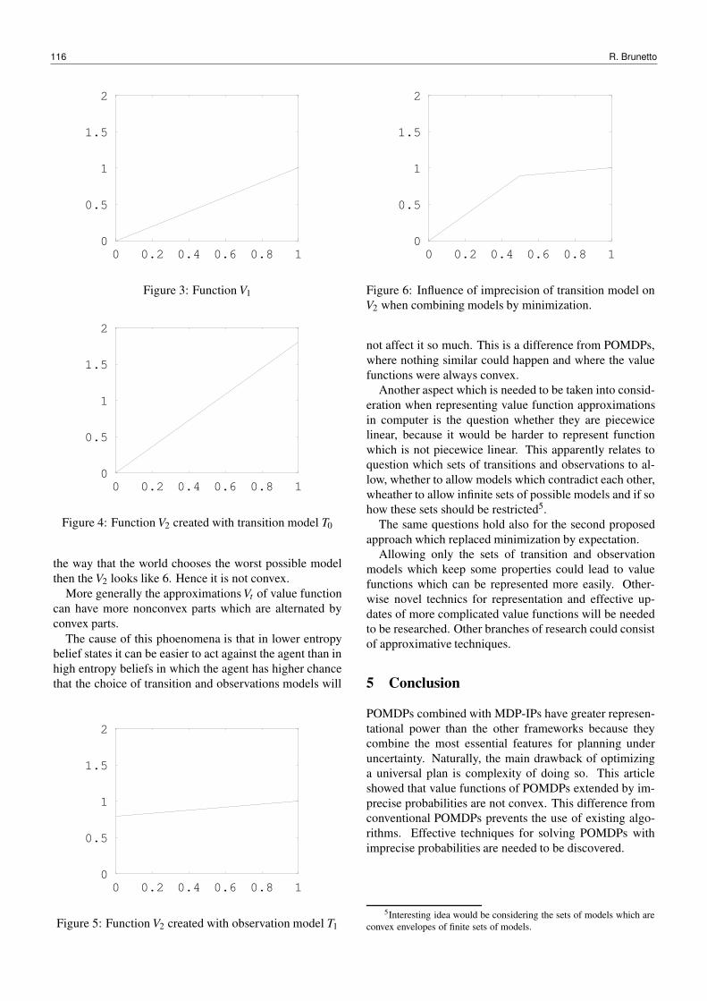
0

0.5

1

1.5

2

0 0.2 0.4 0.6 0.8 1

Figure 3: Function V1

0

0.5

1

1.5

2

0 0.2 0.4 0.6 0.8 1

Figure 4: Function V2 created with transition model T0

the way that the world chooses the worst possible modelthen the V2 looks like 6. Hence it is not convex.

More generally the approximations Vt of value functioncan have more nonconvex parts which are alternated byconvex parts.

The cause of this phoenomena is that in lower entropybelief states it can be easier to act against the agent than inhigh entropy beliefs in which the agent has higher chancethat the choice of transition and observations models will

0

0.5

1

1.5

2

0 0.2 0.4 0.6 0.8 1

Figure 5: Function V2 created with observation model T1

0

0.5

1

1.5

2

0 0.2 0.4 0.6 0.8 1

Figure 6: Influence of imprecision of transition model onV2 when combining models by minimization.

not affect it so much. This is a difference from POMDPs,where nothing similar could happen and where the valuefunctions were always convex.

Another aspect which is needed to be taken into consid-eration when representing value function approximationsin computer is the question whether they are piecewicelinear, because it would be harder to represent functionwhich is not piecewice linear. This apparently relates toquestion which sets of transitions and observations to al-low, whether to allow models which contradict each other,wheather to allow infinite sets of possible models and if sohow these sets should be restricted5.

The same questions hold also for the second proposedapproach which replaced minimization by expectation.

Allowing only the sets of transition and observationmodels which keep some properties could lead to valuefunctions which can be represented more easily. Other-wise novel technics for representation and effective up-dates of more complicated value functions will be neededto be researched. Other branches of research could consistof approximative techniques.

5 Conclusion

POMDPs combined with MDP-IPs have greater represen-tational power than the other frameworks because theycombine the most essential features for planning underuncertainty. Naturally, the main drawback of optimizinga universal plan is complexity of doing so. This articleshowed that value functions of POMDPs extended by im-precise probabilities are not convex. This difference fromconventional POMDPs prevents the use of existing algo-rithms. Effective techniques for solving POMDPs withimprecise probabilities are needed to be discovered.

5Interesting idea would be considering the sets of models which areconvex envelopes of finite sets of models.

116 R. Brunetto

6 Acknowledgments

This research was supported by SVV project number 267314.

References

[1] Delgado K. V., S. Sanner, and L. Nunes de Barros, Efficientsolutions to factored MDPs with imprecise transition proba-bilities, Artificial Intelligence, 175, 1498-1527, 2011

[2] Itoh H., and K. Nakamura, Partially observable Markovdecision processes with imprecise parameters, Artficial In-teligence, 171, 453-490, 2007

[3] Kaelbling L. P., M. L. Littman, and A. R. Cassandra, Plan-ning and acting in partially observable stochastic domains,Artificial Intelligence, 101, 99-134, 1998

[4] Kolobov A., Mausam, and D. S. Weld, Discovering hiddenstructure in factored MDPs, Artificial Intelligence, 189, 19-47, 2012

[5] Pineau J., G. Gordon and S. Thrun, Anytime Point-BasedApproximations for Large POMDPs, Journal of Artificial In-telligence Research 27, 2006

[6] Roy N., G. Gordon and S. Thrun, Finding ApproximatePOMDP Solutions Through Belief Compression, Journal ofArtificial Intelligence Research 23, 2005

Probabilistic Modeling of Dynamic Systems 117

Poster Abstracts

119

Mental map models for edge drawing∗

Martin Duriš and Jana Katreniaková

Faculty of Mathematics, Physics and Informatics, Comenius University Bratislava, Slovakia,mato.duris@gmail.com, katreniakova@dcs.fmph.uniba.sk,

Drawing of graphs is often used for visualization ofstructured information. To make the drawing easy to read(and thus improve the understanding of the underlayingstructures), it should fulfill some aesthetic criteria. Howe-ver, the drawing of graph is mostly not just a static image.The graph can be changed over time – some vertices oredges can be changed, added or removed. The easiest wayof handling the changes is to redraw the graph using thesame algorithm as before. However, in this case even smallchanges to the graph may result in a drawing that is com-pletely different and it is hard for the user to find corres-pondence between the old and new drawings. To make thenew drawing readable, the user must be able to understandthe changes made to the graph and rediscover the structu-res in the new drawing. Therefore, there should be anot-her group of criteria – dynamic criteria, which preservesome properties of the last drawing. The concept of men-tal map was introduced[1] to do this for vertex placement.The mental map captures some important features of thevertex placement (e.g. relative positions up/down/left/rightof vertices). It is said that the mental map is preserved bet-ween timeslices if the changes are acceptable (e.g. all re-lative position remain the same). There are applicationswhere positions of vertices are fixed, for instance if theywere defined by the user or the exact position of the verti-ces is somehow significant. In these cases, the traditionalmental map is useless, since it is trivially preserved. Thedrawing algorithm only finds some routing of the edges.The mental map should capture key features of the edgerouting. However, until now, there was no suitable mo-del of mental map which contains also some informationabout the drawing of edges.

In our work, we introduce two models suitable for pre-serving similarity in routing of edges. We try to followthe intuitive idea of similarity of two polylines. We do notonly define the mental map model, we also provide an al-gorithm that uses the results of the drawing algorithm tocreate new routing of the edges that preserves the mentalmap as it is defined by the model.

The first model of mental map deals with the placementof bends of the polyline. We say, that the mental map ispreserved, if only a constant number of bends (from theprevious edge routing) is changed. The algorithm startswith the new routing (generated by the routing algorithm)and if it does not preserve the mental map, it creates an al-ternative edge routing which has at most k changed bends.The algorithm tries to find the bends that must be changed

∗The research was supported in part by VEGA 1/1085/12

(due to obstacles in the previous routing) and there is lessthan k of them, it tries to make the changes in such a wayto make the routing as similar as possible to the original.Otherwise, a completely new routing has to be used.

The second model is more advanced and it defines anarea, where the edge can be freely routed, i.e., the drawingof the edge must fit into this area. We call this area thecorridor. The corridor should be as small as possible tomake the new drawing similar to the previous routing, ho-wever it needs to be big enough to find a valid routing. Thecorridor can be described as an area between two border-polylines. This makes it easy to compute whether eachpoint from some edge routing is in the corridor and thusthe routing preserves mental map. First idea can be to findsome epsilon neighborhood of the original edge drawing.However the epsilon is not the same for each of the linesegments which form the polyline. Some of them may becontain obstacles, the others may be free. Therefore wemust build the corridor from subcorridors which corres-pond to line segments. We chose some borders of subcor-ridors to be part of the final border of corridor. The easiestway is to build the convex hull of the subcorridors, but it istoo big and does not follow the idea of using a neighbor-hood of the polyline. Therefore, we build the borders usingalpha-edges[2]. Such corridor is scalable and allows us toexpand it if it is not large enough for the drawing algorithmto route the edge inside the corridor. Moreover, since theedge is directly routed using the drawing algorithm, it alsopreserves the static criteria.

Measuring of dynamic aesthetic criteria is hard. We pro-posed measurements based on geometric characteristics ofthe routed edges (polylines). We compared averaged dis-tance between the edge routing before user interaction andafter. Without any mental map, the average distance of thepolylines is 21.86. Using mental map, the average distanceis 17.07 (first model) and 10.99 (second model). If we usea widely used static criterion for edges – the length of theedge – we can see that the results of our models (especiallythe second one) are also good. The first model providesrouting with ratio 1.2 and the second model 1.1.

Literatúra

[1] Eades P., Lai W., Misue K., and Sugiyama K.: Preservingthe Mental Map of a Diagram. Proc. of Compugraphics, 91:24–33, 1991.

[2] Edelsbrunner H., Kirkpatrick D.G., Seidel R.: On the shapeof a set of points in the plane, IEEE Transactions on Infor-mation Theory 29 (4): 551–559, 1983.

ITAT 2013: Workshops, Posters, and Tutorials, p. 120ISBN 978-1490952086, c© 2013 M. Duriš, J. Katreniaková

Can Software Engineers be Liberated from Petri Nets?

Hana Kubátová Dept. of Digital Design, Faculty of Information Technology, Czech Technical University in Prague

Thákurova 9, 160 00 Praha 6, Czech Republic hana.kubatova@fit.cvut.cz

Karel Richta Dept. of Software Engineering, Faculty of Mathematics and Physics, Charles University in Prague

Malostranské nám.25, Praha 1, 118 00, Czech Republic karel.richta@mff.cuni.cz

Tomáš Richta Dept. of Intelligent Systems, Faculty of Information Technology, University of Technology in Brno

Božetěchova 2, 612 66 Brno, Czech Republic irichta@fit.vutbr.cz

Abstract. Petri nets are widely used for the specification of problems, in particular for describing concurrent systems. On the other hand, new versions of the UML specification precisely define the semantics of activity diagrams, and state machines, which can also be used to describe parallel systems. An interesting question is whether we can replace any Petri net machine status describing the same behavior, and vice versa.

The Problem In our case we are in a situation where we want to

describe a network of communicating agents using Petri nets. E.g. we want to define a smart home solution, which consists of a set of agents monitoring and controlling various elements, such as heating, cooling, etc. We are able to describe these agents by Petri nets, and we have a tool that can simulate designed system. On the other hand, there exist available tools that can convert description of the system by UML state diagrams to the target platform implemented as small embedded systems, or, if necessary, to transfer it directly to the hardware implemented using e.g. by FPGA.

Our aim, therefore, was the proposal of a universal procedure that can convert any description by Petri nets to an equivalent description using UML state machines. This would have allow us to simulate virtually the design of communicating agents described by Petri nets, and then transform it into an effective solution based on state diagrams.

Some beginners confuse state diagrams to activity diagrams. The difference between state machines and activity diagrams is important because these two diagrams represent two very different programming paradigms: event-driven programming (state diagrams) and structured programming (activity diagrams).

When creating state diagrams we have to constantly think about possible events. In contrast, in the activity diagrams, the events are secondary things. Natural extension of state diagrams is to allow transitions from any number of states in any number of states. This is however only useful if the system can simultaneously be in several states (regions) together, which means that each state describes only a partial aspect of the overall, global state.

The resulting formalism is known as a Petri net. The reverse procedure simulates transitions in a Petri net with branching in UML. Another extension allows the integration of diagrams, activity diagrams status (Harel). This extension supports the development of software that is both event-driven "workflow" and software-driven process model.

Conclusions In the foregoing chapters we have shown that any Petri

net can be replaced by an equivalent state machine. So it is the base idea that developers can be freed from Petri nets. It's not strict restrictions - Petri nets can be used where there is a description of the network easier to use than using the state machine description.

The conversion allows the integration of flowcharts within Harel state charts and Petri nets. This extension supports the development of software that is both event driven and workflow driven.

Acknowledgment This work has been supported by the Ministry of

Education, Youth and Sports under Research Program No. MSM 6840770014, and also by the grant project of the Czech Grant Agency (GA_CR) No. GA201/09/0990, and also by the AVAST Foundation.

References [1] Girault, C. – Valk, R.: Petri Nets for System

Engineering: A Guide to Modeling Verification, and Applications. Springer-Verlag New York, Inc., Secaucus, NJ, USA,2001.

[2] Richta, T. - Janoušek, V. - Kočí, R.: Code Generation For Petri Nets-Specified Reconfigurable Distributed Control Systems. In: Proceedings of 15th International Conference on Mechatronics –Mechatronika 2012. pp. 263-270. IEEE, Praha 2012.

[3] OMG (February 2009): OMG Unified Modeling Language (OMG UML), Superstructure Version 2.2. URL: http://www.omg.org/spec/UML/2.2/Superstructure/PDF. 2009.

ITAT 2013: Workshops, Posters, and Tutorials, p. 121ISBN 978-1490952086, c© 2013 H. Kubátová, K. Richta, T. Richta

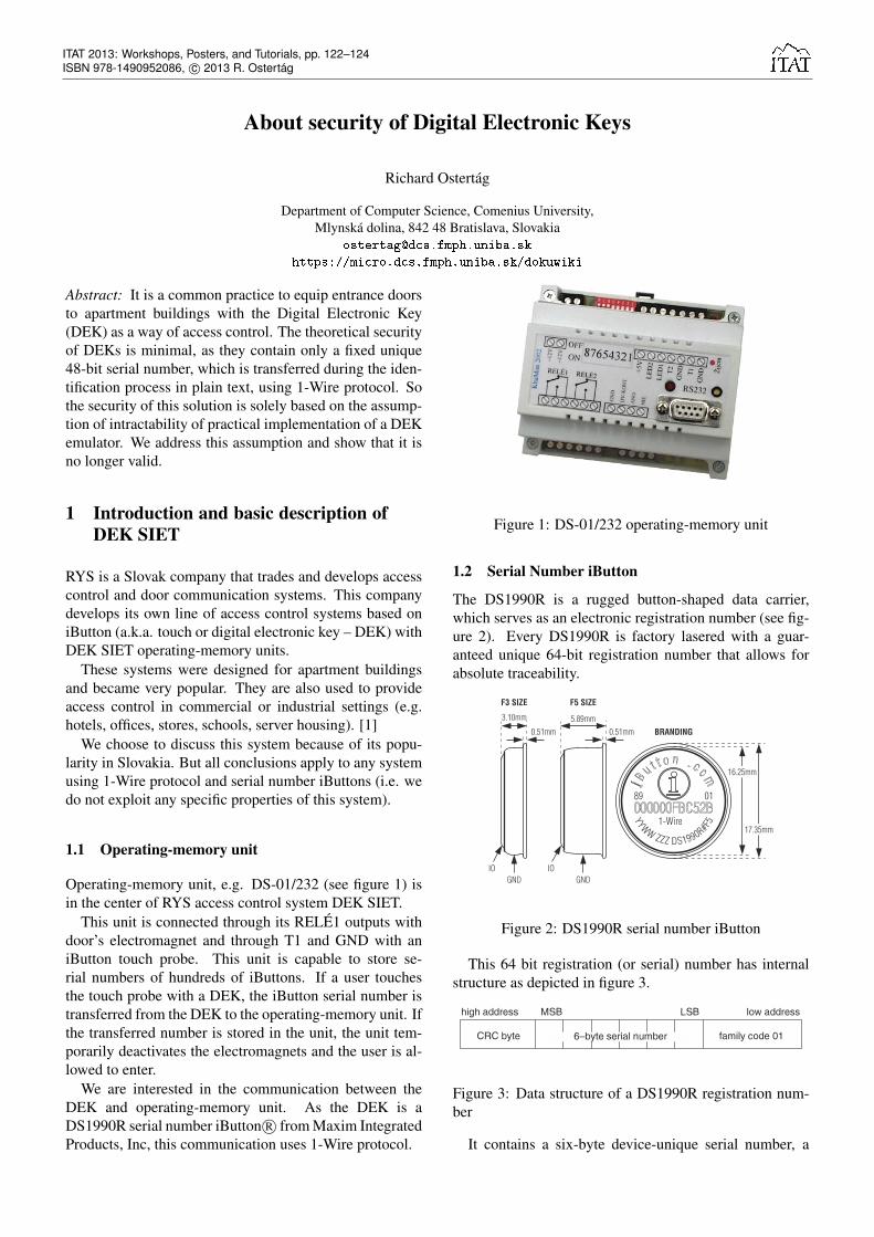
About security of Digital Electronic Keys

Richard Ostertág

Department of Computer Science, Comenius University,Mlynská dolina, 842 48 Bratislava, Slovakia

ostertag@dcs.fmph.uniba.sk

https://micro.dcs.fmph.uniba.sk/dokuwiki

Abstract: It is a common practice to equip entrance doorsto apartment buildings with the Digital Electronic Key(DEK) as a way of access control. The theoretical securityof DEKs is minimal, as they contain only a fixed unique48-bit serial number, which is transferred during the iden-tification process in plain text, using 1-Wire protocol. Sothe security of this solution is solely based on the assump-tion of intractability of practical implementation of a DEKemulator. We address this assumption and show that it isno longer valid.

1 Introduction and basic description ofDEK SIET

RYS is a Slovak company that trades and develops accesscontrol and door communication systems. This companydevelops its own line of access control systems based oniButton (a.k.a. touch or digital electronic key – DEK) withDEK SIET operating-memory units.

These systems were designed for apartment buildingsand became very popular. They are also used to provideaccess control in commercial or industrial settings (e.g.hotels, offices, stores, schools, server housing). [1]

We choose to discuss this system because of its popu-larity in Slovakia. But all conclusions apply to any systemusing 1-Wire protocol and serial number iButtons (i.e. wedo not exploit any specific properties of this system).

1.1 Operating-memory unit

Operating-memory unit, e.g. DS-01/232 (see figure 1) isin the center of RYS access control system DEK SIET.

This unit is connected through its RELÉ1 outputs withdoor’s electromagnet and through T1 and GND with aniButton touch probe. This unit is capable to store se-rial numbers of hundreds of iButtons. If a user touchesthe touch probe with a DEK, the iButton serial number istransferred from the DEK to the operating-memory unit. Ifthe transferred number is stored in the unit, the unit tem-porarily deactivates the electromagnets and the user is al-lowed to enter.

We are interested in the communication between theDEK and operating-memory unit. As the DEK is aDS1990R serial number iButton R© from Maxim IntegratedProducts, Inc, this communication uses 1-Wire protocol.

Figure 1: DS-01/232 operating-memory unit

1.2 Serial Number iButton

The DS1990R is a rugged button-shaped data carrier,which serves as an electronic registration number (see fig-ure 2). Every DS1990R is factory lasered with a guar-anteed unique 64-bit registration number that allows forabsolute traceability.

Figure 2: DS1990R serial number iButton

This 64 bit registration (or serial) number has internalstructure as depicted in figure 3.

Figure 3: Data structure of a DS1990R registration num-ber

It contains a six-byte device-unique serial number, a

ITAT 2013: Workshops, Posters, and Tutorials, pp. 122–124ISBN 978-1490952086, c© 2013 R. Ostertág

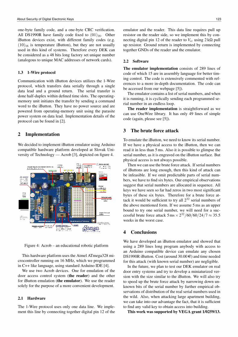
one-byte family code, and a one-byte CRC verification.All DS1990R have family code fixed to (01)16. OtheriButton devices exist, with different family codes (e.g.(10)16 is temperature iButton), but they are not usuallyused in this kind of systems. Therefore every DEK canbe considered as a 48 bits long factory set unique number(analogous to unique MAC addresses of network cards).

1.3 1-Wire protocol

Communication with iButton devices utilizes the 1-Wireprotocol, which transfers data serially through a singledata lead and a ground return. The serial transfer isdone half-duplex within defined time slots. The operating-memory unit initiates the transfer by sending a commandword to the iButton. They have no power source and arepowered from operating-memory unit using the parasitepower system on data lead. Implementation details of theprotocol can be found in [2].

2 Implementation

We decided to implement iButton emulator using Arduinocompatible hardware platform developed at Slovak Uni-versity of Technology — Acrob [3], depicted on figure 4.

Figure 4: Acrob – an educational robotic platform

This hardware platform uses the Atmel ATmega328 mi-crocontroller running on 16 MHz, which we programmedin C++ like language, using standard Arduino IDE [4].

We use two Acrob devices. One for emulation of thedoor access control system (the reader) and the otherfor iButton emulation (the emulator). We use the readersolely for the purpose of a more convenient development.

2.1 Hardware

The 1-Wire protocol uses only one data line. We imple-ment this line by connecting together digital pin 12 of the

emulator and the reader. This data line requires pull upresistor on the reader side, so we implement this by con-necting digital pin 12 of the reader to Vcc using 2 kΩ pullup resistor. Ground return is implemented by connectingtogether GNDs of the reader and the emulator.

2.2 Software

The emulator implementation consists of 289 lines ofcode of which 15 are in assembly language for better tim-ing control. The code is extensively commented with ref-erences to a more in-depth documentation. The code canbe accessed from our webpage [5]).

The emulator contains a list of serial numbers, and whenit is running, it is cyclically sending each programmed se-rial number in an endless loop.

The reader implementation is straightforward as wecan use OneWire library. It has only 49 lines of simplecode (again, please see [5]).

3 The brute force attack

To emulate the iButton, we need to know its serial number.If we have a physical access to the iButton, then we canread it in less than 5 ms. Also it is possible to glimpse theserial number, as it is engraved on the iButton surface. Butphysical access is not always possible.

Then we can use the brute force attack. If serial numbersof iButtons are long enough, then this kind of attack canbe infeasible. If we omit predictable parts of serial num-bers, we have to find six bytes. Our empirical observationssuggest that serial numbers are allocated in sequence. Allkeys we have seen so far had zeros in two most significantbytes of these six bytes. Therefore for a brute force at-tack it would be sufficient to try all 232 serial numbers ofthe above mentioned form. If we assume 5 ms as an upperbound to try one serial number, we will need for a suc-cessful brute force attack 5ms× 232/60/60/24/7 ≈ 35.5weeks in the worst case.

4 Conclusions

We have developed an iButton emulator and showed thatusing a 289 lines long program anybody with access toan Arduino compatible device can emulate any chosenDS1990R iButton. Cost (around 30.00AC) and time neededfor this attack (with known serial number) are negligible.

In the future, we plan to test our DEK emulator on realdoor entry systems and try to develop a miniaturized ver-sion with the size similar to the iButton. We will also tryto speed up the brute force attack by narrowing down un-known bits of the serial number by further empirical ob-servations of distribution of the real serial numbers used inthe wild. Also, when attacking large apartment building,we can take into our advantage the fact, that it is sufficientto find any valid key to obtain access into building.

This work was supported by VEGA grant 1/0259/13.

About Security of Digital Electronic Keys 123

References

[1] RYS: Access control and door entry systems. (http://www.rys.sk/html_eng/english.htm) [Online; accessed1-July-2013].

[2] Maxim Integrated Products, Inc.: Book of iButton standards(application note 937). http://www.maximintegrated.

com/app-notes/index.mvp/id/937 (2002) [Online; ac-cessed 1-July-2013].

[3] Balogh, R.: Acrob - an educational robotic plat-form. AT&P Journal Plus 10 (2010) 6–9 ISSN 1336-5010. http://ap.urpi.fei.stuba.sk/balogh/pdf/

10ATPplusAcrob.pdf [Online; accessed 1-July-2013].[4] Arduino: Arduino software. (http://arduino.cc/en/

main/software) [Online; accessed 1-July-2013].[5] Ostertág, R.: The iButton emulator source code. (https://

micro.dcs.fmph.uniba.sk/iButton.zip) [Online; ac-cessed 1-July-2013].

124 R. Ostertág

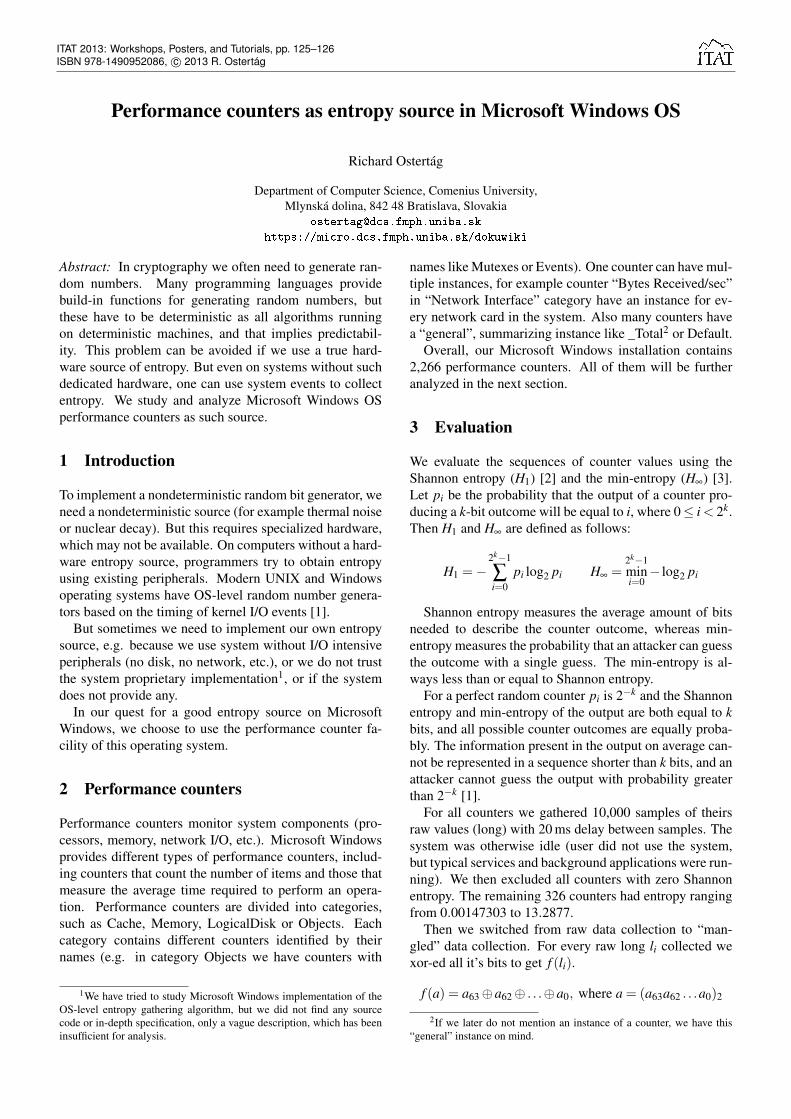
Performance counters as entropy source in Microsoft Windows OS

Richard Ostertág

Department of Computer Science, Comenius University,Mlynská dolina, 842 48 Bratislava, Slovakia

ostertag@dcs.fmph.uniba.sk

https://micro.dcs.fmph.uniba.sk/dokuwiki

Abstract: In cryptography we often need to generate ran-dom numbers. Many programming languages providebuild-in functions for generating random numbers, butthese have to be deterministic as all algorithms runningon deterministic machines, and that implies predictabil-ity. This problem can be avoided if we use a true hard-ware source of entropy. But even on systems without suchdedicated hardware, one can use system events to collectentropy. We study and analyze Microsoft Windows OSperformance counters as such source.

1 Introduction

To implement a nondeterministic random bit generator, weneed a nondeterministic source (for example thermal noiseor nuclear decay). But this requires specialized hardware,which may not be available. On computers without a hard-ware entropy source, programmers try to obtain entropyusing existing peripherals. Modern UNIX and Windowsoperating systems have OS-level random number genera-tors based on the timing of kernel I/O events [1].

But sometimes we need to implement our own entropysource, e.g. because we use system without I/O intensiveperipherals (no disk, no network, etc.), or we do not trustthe system proprietary implementation1, or if the systemdoes not provide any.

In our quest for a good entropy source on MicrosoftWindows, we choose to use the performance counter fa-cility of this operating system.

2 Performance counters

Performance counters monitor system components (pro-cessors, memory, network I/O, etc.). Microsoft Windowsprovides different types of performance counters, includ-ing counters that count the number of items and those thatmeasure the average time required to perform an opera-tion. Performance counters are divided into categories,such as Cache, Memory, LogicalDisk or Objects. Eachcategory contains different counters identified by theirnames (e.g. in category Objects we have counters with

1We have tried to study Microsoft Windows implementation of theOS-level entropy gathering algorithm, but we did not find any sourcecode or in-depth specification, only a vague description, which has beeninsufficient for analysis.

names like Mutexes or Events). One counter can have mul-tiple instances, for example counter “Bytes Received/sec”in “Network Interface” category have an instance for ev-ery network card in the system. Also many counters havea “general”, summarizing instance like _Total2 or Default.

Overall, our Microsoft Windows installation contains2,266 performance counters. All of them will be furtheranalyzed in the next section.

3 Evaluation

We evaluate the sequences of counter values using theShannon entropy (H1) [2] and the min-entropy (H∞) [3].Let pi be the probability that the output of a counter pro-ducing a k-bit outcome will be equal to i, where 0≤ i< 2k.Then H1 and H∞ are defined as follows:

H1 =−2k−1

∑i=0

pi log2 pi H∞ =2k−1mini=0− log2 pi

Shannon entropy measures the average amount of bitsneeded to describe the counter outcome, whereas min-entropy measures the probability that an attacker can guessthe outcome with a single guess. The min-entropy is al-ways less than or equal to Shannon entropy.

For a perfect random counter pi is 2−k and the Shannonentropy and min-entropy of the output are both equal to kbits, and all possible counter outcomes are equally proba-bly. The information present in the output on average can-not be represented in a sequence shorter than k bits, and anattacker cannot guess the output with probability greaterthan 2−k [1].

For all counters we gathered 10,000 samples of theirsraw values (long) with 20 ms delay between samples. Thesystem was otherwise idle (user did not use the system,but typical services and background applications were run-ning). We then excluded all counters with zero Shannonentropy. The remaining 326 counters had entropy rangingfrom 0.00147303 to 13.2877.

Then we switched from raw data collection to “man-gled” data collection. For every raw long li collected wexor-ed all it’s bits to get f (li).

f (a) = a63⊕a62⊕ . . .⊕a0, where a = (a63a62 . . .a0)2

2If we later do not mention an instance of a counter, we have this“general” instance on mind.

ITAT 2013: Workshops, Posters, and Tutorials, pp. 125–126ISBN 978-1490952086, c© 2013 R. Ostertág

Then eight such bits f (l1), f (l2), . . . , f (l8) from eightlongs l1, l2, . . . , l8 were grouped into one byte m(l1, . . . , l8).

m(l1, l2, . . . , l8) =(

f (l1) f (l2) . . . f (l8))

2

This way we again collected 10,000 byte samples fromevery (non-zero entropy) counter with 20 ms delay be-tween raw samples on an otherwise idle system. Then weselected only counters with entropy and min-entropy of atleast 7, resulting in 62 counters.

We also wanted to evaluate stability of entropy and thuswe introduce floating entropy. Floating entropy is calcu-lated as a mean of entropies of consecutive overlappingwindows of length 1,000 with step one. Standard devia-tion of floating entropy is standard deviation of entropiesof all windows.

Only counters with floating Shannon entropy of at least7.8 and standard deviation less than 0.017 and floatingmin-entropy at least 6.55 proceeded to the next round.This way we had obtained 16 promising counters listedin table 1.

Category NameLogicalDisk % Idle TimePhysicalDisk % Idle TimeProcess Elapsed TimeProcess IO Other Operations/secProcessor % C3 TimeProcessor C3 Transitions/secProcessor % Idle TimeProcessor % Privileged TimeProcessor Information % C3 TimeProcessor Information DPCs Queued/secProcessor Information % Priority TimeSynchronization AcqShrdLite/secSynchronization IPI Send Broadcast Req./secSystem System Calls/secThread Context Switches/secThread % Processor Time

Table 1: Promising performance counters based on thefirst experiment. Counters passing also thresholds of thesecond experiment are highlighted.

We further analyzed these promising counters by sam-pling them on another personal computer. Shannon andmin-entropies from this second experiment are shown infigure 1.

In last round we excluded “Process, IO Other Opera-tions/sec”, “Processor, % Privileged Time” and “Synchro-nization, IPI Send Broadcast Requests/sec” as theirs min-entropy, this time, was below threshold of 7 bits. “Process,Elapsed Time” and “Processor, C3 Transitions/sec” and“Processor, % Idle Time” counters were also disqualified,because they had standard deviation of floating Shannonentropy greater than 0.019.

0 5 10 15

2

4

6

8

Entr

opy

Counters from table 1

Min-entropy

Shannon entropy

Figure 1: Shannon and min-entropies of counters in table1 evaluated on a different computer.

The remaining ten counters had entropy (Shannon andmin) of at least 7, floating Shannon entropy of at least 7.79with standard deviation less than 0.019 and floating min-entropy of at least 6.5 with standard deviation less than0.16 in two experiments on different computers. In thesecond experiment we have slightly relaxed thresholds toaccount for small disturbance in measured properties.

4 Conclusions

We have analyzed 2,266 performance counters of Mi-crosoft Windows operating system and have found amongthem ten promising counters, highlighted in table 1, withhigh and stable entropy.

In future, we plan to study correlation between selectedcounters (e.g. we expect that LogicalDisk and PhysicalD-isk will be highly correlated) with the aim to exclude re-dundant counters. Also we plan to test behavior of thesecounters on different versions of Microsoft Windows. Wealso want to study influence of virtualization of underly-ing OS on these counters and their other properties likethe Markov-Rényi min entropy.

This work was supported by VEGA grant 1/0259/13.

References

[1] Hamburg, M., Kocher, P., Marson, M.E.: Analy-sis of Intel’s Ivy Bridge digital random number genera-tor. http://cryptography.com/public/pdf/Intel_

TRNG_Report_20120312.pdf (2012) [Online; accessed 1-July-2013].

[2] Shannon, C.E.: A mathematical theory of communication.The Bell System Technical Journal 27 (1948) 379–423, 623–656

[3] Barker, E.B., Kelsey, J.M.: Recommendation for RandomNumber Generation Using Deterministic Random Bit Gen-erators. US Department of Commerce, National Institute ofStandards and Technology, Computer Security Division, In-formation Technology Laboratory (2012)

126 R. Ostertág

Tutorial Materials

127

Bezdrôtové siete senzorov a aktuátorov - od teórie k aplikáciám

Michal Hodoň Katedra Technickej kybernetiky,

Fakulta riadenia a informatiky, Žilinská univerzita v Žiline,

Univerzitná 8215/1, 010 26 Žilina

Juraj Miček, Ondrej Karpiš, Peter Ševčík Katedra Technickej kybernetiky, Fakulta riadenia a informatiky,

Žilinská univerzita v Žiline, Univerzitná 8215/1, 010 26 Žilina

Abstract. V súčasnosti sa často stretávame s pojmami „Prevasive Computing, Mobile Computing, Ubiquitous Computing (Ubicomp), Ambient Intelligence, Smart Dust, Internet of Things“, ktoré naznačujú, že v najbližšej dobe je možné očakávať ďalší masívny prienik prostriedkov a systémov informačných technológií do všetkých oblastí ľudskej spoločnosti. Zariadenia schopné snímať parametre prostredia budov, monitorovať aktivitu jednotlivca, monitorovať a ovládať technické systémy, umožňovať vyžiadanú asistenciu pri náročnejších činnostiach a mnohé ďalšie sa dnes stávajú realitou. Väčšina týchto zariadení je schopná vzájomnej komunikácie a priamo, alebo prostredníctvom prístupových zariadení sú integrované do siete Internet. Narastá množstvo dostupných informácií. Čas na získanie relevantných dát je dnes mimoriadne krátky. Menia sa paradigmy spracovania dát. Každým dňom sa rozširujú aplikačné oblasti prostriedkov informačných technológií. To čo nebolo ešte včera realizovateľné je dnes komerčne používané.

Jednou z oblastí, ktorá už dnes predstavuje úspešne využívanú technológiu je oblasť bezdrôtových senzorických sietí, (Wireless Sensor Network, WSN). Práve bezdrôtovým sieťam senzorov je venovaný tento príspevok. Na základe predchádzajúceho vývoja je možné predpokladať, že v najbližšom desaťročí sa počet aplikácií WSN mnohonásobne zvýši. Aj z tohto dôvodu je príspevok venovaný popisu WSN, možnostiam ich využitia a niektorým otázkam spojeným s návrhom prvku siete, siete senzorov a možných aplikácií. V druhej časti príspevku sú uvedené úspešné i menej úspešné aplikácie popisovanej technológie, ktoré vznikli na našom pracovisku.

1 Úvod V posledných rokoch sa bezdrôtovým sieťam senzorov

venuje stále väčšia pozornosť. Uvedený stav súvisí najmä: • s pokrokmi technológie v oblasti výroby

mikroelektronických systémov, ktorá umožňuje integrovať v jednom obvode výkonný systém spracovania dát,

• s pokrokmi v oblasti snímačov, najmä vývoj nových snímacích prvkov na báze mikro-elektoro-mechanických systémov, MEMS,

• s pokrokmi v oblasti komunikačných technológií, spoľahlivé digitálne RF-komunikačné systémy krátkeho dosahu s nízkou energetickou náročnosťou,

• s pokrokmi v oblasti zdrojov energie a systémov zberu energie z okolia.

Je zrejmé, že pokiaľ technologické možnosti výroby základných komponentov WSN nedosiahli kritickú hranicu, nebolo možné očakávať široké nasadzovanie technológií

WSN v rôznych aplikačných oblastiach. Napriek tomu je možné spomenúť jednu oblasť aplikácií, kde ekonomické hľadiská nehrajú dominantnú úlohu. Je to vojenská oblasť, v ktorej je možné sledovať snáď prvé nasadenie WSN na monitorovanie pohybu vojsk. Spomeňme systém označovaný ADSID (Air Delivered Seismic Intrusion Detector), ktorý bol používaný jednotkami US Air Force vo vietnamskej vojne. Pre zaujímavosť pripomeňme, že každý senzor bol približne 120 cm dlhý, jeho priemer mal cca 23 cm a vážil 17 kg. Senzor obsahoval citlivý seizmometer, ktorý bol schopný zaznamenávať vibrácie spôsobené pohybujúcimi sa vozidlami a osobami. Senzory boli rozmiestnené popri známej Ho Či Min-ovej ceste. Zaznamenané informácie boli vysielané priamo do lietadiel, ktoré lietali nad monitorovanou oblasťou. Pripomeňme tiež systém používaný na monitorovanie pohybu ponoriek v 50-tych rokoch minulého storočia. Systém s označením SOSUS, Sound Sourveillance System, bol vyvinutý pre armádne účely USA a využíval sieť hydrofónov rozmiestnených v Atlantickom a Tichom oceáne. Dnes je táto sieť používaná na sledovanie podmorského života a vulkanickej aktivity.

No až technologické pokroky v poslednom období podnietili vznik nových zaujímavých ekonomicky efektívnych aplikácií.

Bezdrôtová sieť senzorov pozostáva z priestorovo rozložených autonómnych snímacích prvkov, ktoré navzájom komunikujú. Sú rozmiestnené v monitorovanej oblasti a priebežne vyhodnocujú stav sledovaného objektu. Pojem objekt chápeme v najširšom slova zmysle a môže predstavovať strážený priestor, diagnostikovanú výrobnú linku, dopravný prostriedok, či živú bytosť. V súčasnosti podľa [1] až 99% inštalovaných senzorov komunikuje prostredníctvom vodičov. Predpokladá sa, že v nasledujúcich 10-tich rokoch budú WSN predstavovať nie viac než 10 % všetkých inštalovaných senzorov. V súlade s [1] a [2] uveďme, že pri využití WSN klesajú oproti tradičným riešeniam finančné náklady na inštaláciu a údržbu.

Európska komisia podporila výskumnú a vývojovú činnosť, ako aj nové aplikácie WSN v rámci siedmeho rámcového programu (7FP) v oblasti informačno-komunikačných technológií, 7FP-ICT. Pre roky 2007 až 2013 je celkový objem financií na úrovni 50 mld. €. V poslednom období 2010 až 2012 podporila EK výskum WSN najmä prostredníctvom prvej výzvy „Pervazívne a

ITAT 2013: Workshops, Posters, and Tutorials, pp. 128–135ISBN 978-1490952086, c© 2013 M. Hodon, J. Micek, O. Karpiš, P. Ševcík

dôverné siete a obslužná infraštruktúra“. Na podporu výskumu v rámci spomenutej výzvy vyčlenila EK finančný objem 625 mil. €. V rámci 6-tej výzvy „Informačno-komunikačné technológie pre nízko-uhlíkovú ekonomiku“ bol definovaný cieľ 6.7 „Spolupracujúce systémy pre energeticky efektívnu a udržateľnú mobilitu“, ktorý je venovaný aj využitiu WSN v oblasti dopravy a je podporený finančným objemom 40 mil. €. V rámci podpory medzinárodnej spolupráce EÚ-Brazília bol vyčlenený finančný objem 5 mil. € na podporu spoločných výskumných aktivít v 5-tich špecifikovaných oblastiach, medzi ktoré patria i problémové okruhy z oblasti „WSN pri monitorovaní a riadení zložitých a rozsiahlych systémov“. Táto výzva bola smerovaná na vývoj nových metód parametrizácie, autokonfigurácie, adaptivity, autolokalizácie, optimalizácie, prevádzky v prostredí s vysokou úrovňou rušenia a mnohých ďalších, ktoré by mali byť implementované v pokročilých bezdrôtových sieťach senzorov. Ďalšie výzvy ako napr. podpora medzinárodnej spolupráce EÚ-Japonsko alebo výzvy súvisiace s programom Horizon 2020 sú smerované na riešenie rôznych čiastkových problémov sietí WSN.

Pripomeňme, že najväčší finančný objem (625 mil. € z celkových 2 422 mil. € venovaných 7FP ICT pre roky 2010 - 2012) bol vyčlenený práve na riešenie problémov dotýkajúcich sa výskumu WSN. Za predpokladu, že vyčlenené finančné prostriedky budú účelne využité môžeme v najbližšom období očakávať mimoriadne významný pokrok v oblasti vývoja WSN a tvorby nových efektívnych aplikácií s prienikom do komerčných oblastí.

Záverom je možné konštatovať, že problematika WSN sa dostáva do popredia záujmu aj v európskom výskumnom priestore o čom svedčia mnohé zaujímavé aplikácie [3], [4], [5].

2 Aplikačné oblasti Bezdrôtové siete senzorov, ako priestorovo distribuované

siete tvorené relatívne jednoduchými vzájomne spolupracujúcimi prvkami majú veľký aplikačný potenciál vo vojenských, priemyselných, dopravných, environmentálnych a mnohých ďalších oblastiach.

V nasledujúcich rokoch je možné očakávať ich významné rozšírenie za predpokladu, že budú úspešne doriešené niektoré otázky súvisiace s komunikačnými protokolmi a ich štandardizáciou, efektívnymi zdrojmi energie, ktoré budú schopné zabezpečiť až 20 rokov autonómnej prevádzky uzlov siete a ďalšími pokrokmi v oblasti technológie výroby nízkopríkonových mikroelektronických prvkov.

Ako už bolo spomenuté v úvode jedna z prvých aplikačných oblastí bola tvorená vojenskými aplikáciami (Military). Práve vo vojenskej oblasti sa vyskytuje množstvo úloh spojených s monitorovaním územne rozľahlých oblastí, pričom ekonomické hľadiská zavádzania nových technológií nie sú až natoľko prioritné ako v iných odvetviach hospodárstva.

Spomeňme aspoň systémy navádzania a sledovania cieľa, systémy na detekciu pohybu a identifikáciu druhu bojových prostriedkov, monitorovanie bojového poľa (battlefield surveillance) aplikácie WSN v súvislosti s monitorovaním a ovládaním mínových polí, detekciu

nukleárnych, biologických a chemických útokov (nuclear, biological and chemical attack detection) a mnohé ďalšie, [6].

Ďalšie zaujímavé aplikácie WSN je možné nájsť pri monitorovaní a ochrane životného prostredia. Monitorovanie prostredia patrí dnes snáď medzi najčastejšie aplikácie bezdrôtových sietí senzorov. Práve tieto aplikácie si vyžadujú použitie veľkého počtu lacných snímacích prvkov, ktoré je možné jednoducho rozmiestniť do sledovanej oblasti. Ako najčastejšie aplikácie je možné uviesť monitorovanie pohybu ľadovcov, monitorovanie a ochrana lesa pred požiarmi, nepovoleným výrubom, pytliakmi, varovné systémy pred záplavami a ďalšími prírodnými katastrofami, sledovanie zmien mikroklímy, intenzity slnečného žiarenia a množstvo ďalších zaujímavých aplikácií.

Ďalšou perspektívnou aplikačnou oblasťou bezdrôtových senzorických sietí je oblasť starostlivosti o zdravie, záchrana služba a asistenčné systémy (e-Helath). Je zrejmé, že s využitím technológií WSN je možné zvýšiť súčasnú úroveň monitorovania pacientov, ako aj úroveň zdravotnej starostlivosti. Ako príklad uveďme monitorovanie vitálnych funkcií pacientov v nemocnici. Tieto monitorovacie systémy umožňujú pohyb pacienta pri zachovaní všetkých funkcií statických systémov. Pripomeňme oblasť starostlivosti o staršiu generáciu, prípadne o ľudí s telesným postihnutím, ktorým moderné technológie dovoľujú zvýšiť kvalitu života. V tejto oblasti by bolo možné nájsť mnoho zaujímavých a inšpiratívnych príkladov.

S využitím technológie WSN sa dnes často stretneme v dopravných aplikáciách. Pri monitorovaní a riadení dopravy sú zdroje informácií priestorovo rozptýlené v rozľahlej oblasti. Komplexný prehľad o stave dopravy je možné získať len na základe informácií získaných z veľkého počtu vhodne rozmiestnených snímačov. Problematika monitorovania a riadenia dopravy preto prirodzenie smeruje aj do oblasti aplikácií senzorických sietí.

Spomeňme ešte aplikácie WSN technológií v priemysle. V priemyselných aplikáciách sa najčastejšie stretávame s úlohami monitorovania výroby, pri riadení skladového hospodárstva, prípadne dnes už častejšie, s riadením technologických procesov. Pripomeňme, že v prípade aplikácií v riadení technologických procesov sa často stretávame s pojmami „bezdrôtová sieť senzorov a akčných členov“, „Wireless Sensor and Actuator Networks“ – WSAN, prípadne tiež „priemyselná bezdrôtová sieť senzorov“,„Industrial Wireless Sensor Networks“, IWSN.

Poznamenajme, že popísané aplikácie tvoria len malú oblasť celého aplikačného priestoru WSN. Neboli spomenuté viaceré aplikačné oblasti, s ktorými sa dnes v praxi často stretneme – automatizácia budov, monitorovanie produktovodov, zabezpečovacie systémy, poľnohospodárstvo a mnohé ďalšie.

3 Základné problémy Je zrejmé, že bezdrôtová sieť senzorov je tvorená

veľkým množstvom uzlov „nodov“, ktoré sú rozmiestnené v monitorovanej oblasti. Senzorické uzly bývajú rozmiestnené náhodne, alebo do vopred definovaných

Bezdrôtové siete senzorov a aktuátorov—od teórie k aplikáciám 129

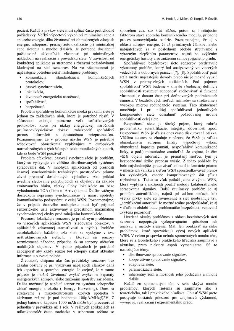
pozícií. Každý z prvkov siete musí spĺňať často protichodné požiadavky. Veľký výpočtový výkon pri minimálnej cene a spotrebe energie, dlhá životnosť pri obmedzených zdrojoch energie, schopnosť presnej autolokalizácie pri minimálnej cene riešenia a mnoho ďalších. Je potrebné dosiahnuť požadované užívateľské vlastnosti pri minimálnych nákladoch na realizáciu a prevádzku siete. V závislosti od konkrétnej aplikácie sa stretneme s rôznymi požiadavkami kladenými na sieť senzorov. No vo všeobecnosti je najčastejšie potrebné riešiť nasledujúce problémy: • komunikácia: štandardizácia komunikačných

protokolov, • časová synchronizácia, • lokalizácia, • životnosť: energetická náročnosť, • spoľahlivosť, • bezpečnosť. Problém spoľahlivej komunikácie medzi prvkami siete je

jednou zo základných úloh, ktoré je potrebné riešiť. V súčasnosti existuje pomerne veľa sofistikovaných protokolov, ktoré pri nízkej energetickej náročnosti prijímačov/vysielačov dokážu zabezpečiť spoľahlivý prenos informácií s dostatočnou priepustnosťou. Poznamenajme, že v procese návrhu WSN je potrebné rešpektovať obmedzenia vyplývajúce z európskych normalizačných a tých štátnych telekomunikačných autorít, kde sa bude WSN používať.

Problém efektívnej časovej synchronizácie je problém, ktorý sa vyskytuje vo väčšine distribuovaných systémov spracovania dát. V mnohých aplikáciách od presnosti časovej synchronizácie technických prostriedkov priamo závisí presnosť dosiahnutých výsledkov. Ako príklad uveďme sledovanie pohybujúcich sa objektov na základe emitovaného hluku, všetky úlohy lokalizácie na báze vyhodnotenia TOA (Time of Arrive) a pod. Ďalším vážnym dôsledkom nepresnej synchronizácie je nárast spotreby komunikačného podsystému v celej WSN. Poznamenajme, že v prípade časového multiplexu musí byť prijímač senzorického uzla aktivovaný s predstihom maximálnej synchronizačnej chyby pred zahájením komunikácie.

Presnosť lokalizácie senzorov je primárnym problémom vo viacerých aplikáciách WSN (sledovanie objektov, v aplikáciách zdravotnej starostlivosti a iných.). Problém autolokalizácie každého uzla siete sa vyskytne v tzv. neštruktúrovaných sieťach, v ktorých sú senzory rozmiestnené náhodne, prípadne ak sú senzory súčasťou mobilných objektov. V týchto prípadoch je potrebné zabezpečiť aby každý senzor bol schopný získať aktuálnu informáciu o svojej polohe.

Životnosť, chápaná ako čas prevádzky senzorov bez zásahu obsluhy je pri využívaní napájacích článkov daná ich kapacitou a spotrebou energie. Je zrejmé, že v tomto prípade je možné životnosť zvýšiť zvýšením kapacity energetických zdrojov, alebo znížením spotreby zariadenia. Ďalšia možnosť je napájať senzor zo systému schopného získať energiu z okolia ( Energy Harvesting). Dnes sa stretávame s mikrokontrolérmi ktorých spotreba v aktívnom režime je pod hodnotou 100µA/MHz@3V. Z jednej batérie o kapacite 1000 mAh môže byť procesorová jednotka v prevádzke až 1 rok. V reálnych aplikáciách sa mikrokontrolér často nachádza v úspornom režime so

spotrebou cca. sto krát nižšou, potom sa limitujúcim faktorom stáva spotreba komunikačného modulu, prípadne proces samovybíjania batérie. Poznamenajme, že aj v oblasti zdrojov energie, či už primárnych článkov, alebo nabíjateľných sa v poslednom období stretávame s výrazným zlepšením parametrov, najmä so zvýšením energetickej hustoty a so znížením samovybíjacieho prúdu.

Spoľahlivosť bezdrôtovej siete senzorov predstavuje významný problém, ktorý bol analyzovaný vo viacerých vedeckých a odborných prácach [7], [8]. Spoľahlivosť patrí stále medzi najčastejšie dôvody prečo nie je možné využiť WSN v priemyselných aplikáciách. Pod pojmom spoľahlivosť WSN budeme v zmysle všeobecnej definície spoľahlivosti rozumieť schopnosť zachovávať si funkčné vlastnosti v danom čase pri definovaných podmienkach činnosti. V bezdrôtových sieťach snímačov sa stretávame s vysokou mierou redundancie systému. Táto skutočnosť umožňuje i pri nižšej spoľahlivosti jednotlivých komponentov siete dosiahnuť požadovanej úrovne spoľahlivosti celej siete.

Bezpečnosť siete je široký pojem, ktorý zahŕňa problematiku autentifikácie, integrity, dôvernosti apod. Bezpečnosť WSN je ďalšia dnes často diskutovaná otázka. Väčšina autorov sa zhoduje v názore, že WSN je vďaka obmedzeným zdrojom (nízky výpočtový výkon, obmedzená kapacita pamätí, nespoľahlivé komunikačné linky, a pod.) mimoriadne zraniteľná. Je zrejmé, že čím väčší objem informácií je prenášaný sieťou, tým je bezpečnostné riziko prenosu vyššie. Z tohto pohľadu by bolo najvhodnejšie spracovávať snímané informácie priamo v mieste ich vzniku a sieťou WSN sprostredkovávať prenos len výsledných, značne komprimovaných dát (fúzia rozhodnutí). Takto sa však potlačí jedna z výhod WSN, ktorá vyplýva z možnosti použiť metódy kolaboratívneho spracovania signálov. Ďalší zaujímavý problém je aj problém autentifikácie, najmä pri ad-hoc sieťach, kde všetky prvky siete sú rovnocenné a sieť neobsahuje tzv. „certifikačnú autoritu“. Je možné reálne predpokladať, že aj v ďalšom období bude problematike bezpečnosti venovaná zvýšená pozornosť.

Uvedené okruhy problémov z oblasti bezdrôtových sietí senzorov nepopisujú vyčerpávajúcim spôsobom ich analýzu a metódy riešenia. Mali len poukázať na šírku problémov, ktoré sprevádzajú vývoj nových aplikácií WSN. V celom príspevku nebolo spomenutých mnoho tém, ktoré sú z teoretického i praktického hľadiska zaujímavé a aktuálne, preto niektoré aspoň vymenujeme. Sú to nasledujúce témy: • distribuované spracovanie signálov, • kooperatívne spracovanie signálov, • adaptivita siete, • parametrizácia siete, • inherentný šum a možnosti jeho potlačenia a mnohé

ďalšie. Každá zo spomenutých tém v sebe skrýva mnoho

problémov, ktorých riešenia sú zaujímavé ako z teoretického, tak i praktického hľadiska. Oblasť WSN preto poskytuje dostatok priestoru pre zaujímavú výskumnú, vývojovú, realizačnú i experimentálnu prácu.

130 M. Hodon, J. Micek, O. Karpiš, P. Ševcík

4 Prehľad vybratých aplikácií WSN Problematika návrhu a realizácie rôznych prvkov WSN

je na Katedre technickej kybernetiky (KTK) riešená od roku 2008, kedy bol navrhnutý prvý senzor pre monitoring rôznych parametrov dopravy v rámci riešenej problematiky inteligentných dopravných systémov. Od tej doby bolo realizovaných viacero zaujímavých prototypov z rôznych aplikačných oblastí, orientovaných primárne na monitoring parametrov dopravy a životného prostredia. Okrem toho bolo vyvinutých zopár prototypov aj pre oblasť Military i e-Health.

Pri praktickej realizácii senzorov bolo nutné okrem základných problémov popísaných vyššie riešiť aj ďalšie vlastnosti parametrizácie senzorov, ako sú výpočtový výkon senzora, cena, energetická nenáročnosť/životnosť senzora, bezpečnosť komunikácie, odolnosť voči poruchám, a pod.

Mnohé z uvedených požiadaviek si navzájom odporujú. Zvyšovaním výpočtového výkonu narastá energetická náročnosť, ako aj cena senzora. Zvýšenie zabezpečenia prenosu vyžaduje väčší výpočtový výkon. Zvýšená odolnosť voči poruchám zvyčajne negatívne ovplyvňuje cenu produkcie. Nie je teda možné vyvinúť dostatočne univerzálny prvok, ktorý bude optimálny z hľadiska všetkých uvedených požiadaviek. Naviac je potrebné pripomenúť, že rôzne aplikácie kladú rôznu váhu na splnenie jednotlivých požiadaviek. Problematika návrhu senzorických prvkov je popísaná v [10]. Autori navrhujú pri vývoji využívať triedu všeobecne použiteľných modulov a aplikačne orientovaných nosičov nosných dosiek - modulov (carriers) a takto dosiahnuť vysoký stupeň univerzálnosti a možnosti používať vyvinuté systémy v čo najširšej množine rôznych aplikácií. Odhliadnuc od hardvérovej platformy a druhu aplikácie každý sensor node WSN musí byť schopný realizovať tri základné funkcie - zber, predspracovanie a posielanie dát. Zber dát sa vykonáva v časti sensor node, ktorú nazveme podsystém zberu dát.

Podsystém zberu dát je časť sensor node, ktorá je mimoriadne závislá od požiadaviek konkrétnej aplikácie. Táto časť obsahuje snímacie prvky, ktoré snímajú tie veličiny, ktoré sú relevantné pre riešenie danej úlohy. Je zrejmé, že iné snímacie prvky sú potrebné pre snímanie parametrov cestnej dopravy, iné pre telemonitoring pacientov v zdravotnom zariadení a celkom iné pri monitorovaní sopečnej aktivity. Z tohto dôvodu je obtiažne špecifikovať univerzálne vlastnosti a parametre podsystému na zber dát. Každá aplikácia vyžaduje do istej miery špeciálny, originálny prístup k jej návrhu. Preto sa v praktických aplikáciách stretávame so skutočnosťou, že práve podsystém na zber údajov sa v rámci pilotného projektu špeciálne vyvíja podľa požiadaviek aplikácie.

Na nasledovných prototypoch je možné získať predstavu o aplikačných možnostiach využitia senzorov pre WSN:

4.1 KTK node pre monitoring akustických emisií a vibrácií v dopravných systémoch

Popisovaný senzor bol vyvinutý z dôvodov experimentálneho overovania nových metód kolaboratívneho spracovania signálov najmä vo frekvenčnom rozsahu do 15 kHz pre akustické emisie a do

1000 Hz vibrácie a chvenie so zameraním na energetickú efektívnosť. Zámerom bolo, po umiestnení senzora v blízkosti monitorovanej komunikácie, na základe emitovaného zvuku vozidiel určiť hustotu premávky na danej komunikácii. Senzor bol realizovaný na báze 32-bitového MCU ST32F100, snímací subsystém bol tvorený mikrofónom MCE100, predzosilňovačom, antialising filtrom druhého rádu a zosilňovačom s riaditeľným ziskom v rozsahu 1 až 352. Výstup zo zosilňovača bol privedený na vstup analógovo číslicového prevodníka integrovaného do puzdra MCU. Na snímanie vibrácií bol použitý 3-osí akcelerometer MMA8453 s možnosťou komunikácie prostredníctvom I2C s 12 a 8-bitovým výstupom. Spotreba akcelerometra v aktívnom režime je do 225 uA v závislosti od vibrácií, spotreba využitého MCU v tzv. „Run móde“ je okolo 4.6 mA@8MHz. Množinu snímačov bolo možné rozšíriť prostredníctvom aplikačného konektora. Pamäťový subsystém bol kvôli možnosti uchovania veľkého objemu dát rozšírený o mikroSD kartu. Za účelom experimentálnych prác s rôznymi komunikačnými modulmi bol na základnej doske senzora umiestnený konektor, prostredníctvom ktorého bolo možné k základnému modulu pripojiť komunikačnú jednotku, v našom prípade to boli moduly XBee PRO v pásme 2.4 GHz. Senzor bol realizovaný na dvojvrstvovej doske plošných spojov s rozmermi 38 x 45 mm, obr.1. Na monitorovanie a riadenie WSN bol vyvinutý modul, ktorý sa pripája k personálnemu počítaču prostredníctvom konektora USB, obr.1 dole.

Obr.1 Vyvinutý node s USB modulom

Senzor bol o.i. využitý aj na hodnotenie kvality cestnej siete v rámci Žilinského kraja, keď po nainštalovaní do testovacieho vozidla zaznamenával na integrovanú SD kartu hodnotu vibrácií a hluku vozidla pri prechode cez testovanú komunikáciu.Viac informácií je možné nájsť v [13].

4.2 KTK node pre lokalizáciu snajpera

Miernou modifikáciou architektúry vyššie popísaného KTK nodu bol vyvinutý senzor pre oblasť Military využitý na riešenie problému lokalizácie snajpera v neznámych

Bezdrôtové siete senzorov a aktuátorov—od teórie k aplikáciám 131

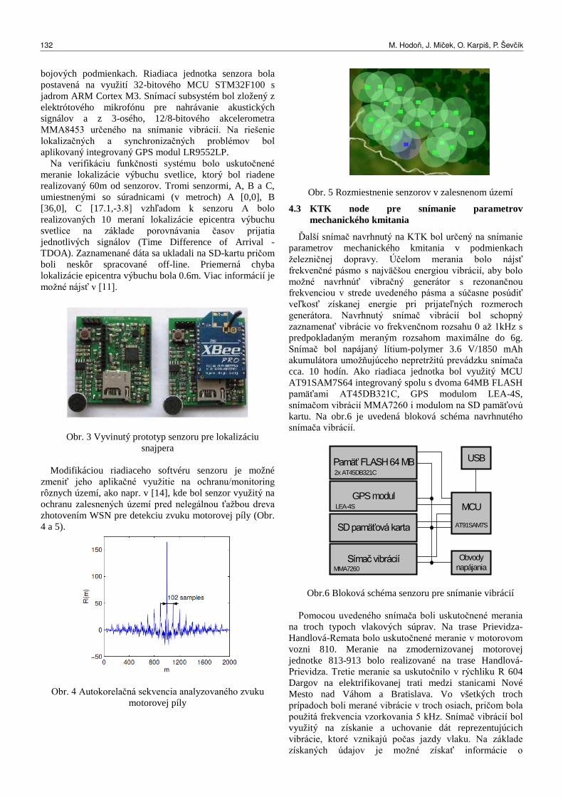
bojových podmienkach. Riadiaca jednotka senzora bola postavená na využití 32-bitového MCU STM32F100 s jadrom ARM Cortex M3. Snímací subsystém bol zložený z elektrótového mikrofónu pre nahrávanie akustických signálov a z 3-osého, 12/8-bitového akcelerometra MMA8453 určeného na snímanie vibrácií. Na riešenie lokalizačných a synchronizačných problémov bol aplikovaný integrovaný GPS modul LR9552LP.

Na verifikáciu funkčnosti systému bolo uskutočnené meranie lokalizácie výbuchu svetlice, ktorý bol riadene realizovaný 60m od senzorov. Tromi senzormi, A, B a C, umiestnenými so súradnicami (v metroch) A [0,0], B [36,0], C [17.1,-3.8] vzhľadom k senzoru A bolo realizovaných 10 meraní lokalizácie epicentra výbuchu svetlice na základe porovnávania časov prijatia jednotlivých signálov (Time Difference of Arrival - TDOA). Zaznamenané dáta sa ukladali na SD-kartu pričom boli neskôr spracované off-line. Priemerná chyba lokalizácie epicentra výbuchu bola 0.6m. Viac informácií je možné nájsť v [11].

Obr. 3 Vyvinutý prototyp senzoru pre lokalizáciu snajpera

Modifikáciou riadiaceho softvéru senzoru je možné

zmeniť jeho aplikačné využitie na ochranu/monitoring rôznych území, ako napr. v [14], kde bol senzor využitý na ochranu zalesnených území pred nelegálnou ťažbou dreva zhotovením WSN pre detekciu zvuku motorovej píly (Obr. 4 a 5).

Obr. 4 Autokorelačná sekvencia analyzovaného zvuku motorovej píly

Obr. 5 Rozmiestnenie senzorov v zalesnenom území

4.3 KTK node pre snímanie parametrov mechanického kmitania

Ďalší snímač navrhnutý na KTK bol určený na snímanie parametrov mechanického kmitania v podmienkach železničnej dopravy. Účelom merania bolo nájsť frekvenčné pásmo s najväčšou energiou vibrácií, aby bolo možné navrhnúť vibračný generátor s rezonančnou frekvenciou v strede uvedeného pásma a súčasne posúdiť veľkosť získanej energie pri prijateľných rozmeroch generátora. Navrhnutý snímač vibrácií bol schopný zaznamenať vibrácie vo frekvenčnom rozsahu 0 až 1kHz s predpokladaným meraným rozsahom maximálne do 6g. Snímač bol napájaný lítium-polymer 3.6 V/1850 mAh akumulátora umožňujúceho nepretržitú prevádzku snímača cca. 10 hodín. Ako riadiaca jednotka bol využitý MCU AT91SAM7S64 integrovaný spolu s dvoma 64MB FLASH pamäťami AT45DB321C, GPS modulom LEA-4S, snímačom vibrácií MMA7260 i modulom na SD pamäťovú kartu. Na obr.6 je uvedená bloková schéma navrhnutého snímača vibrácií.

Pamäť FLASH 64 MB2x AT45DB321C

GPS modulLEA-4S

SD pamäťová karta

Símač vibráciíMMA7260

MCU

AT91SAM7S

Obvodynapájania

USB

Obr.6 Bloková schéma senzoru pre snímanie vibrácií Pomocou uvedeného snímača boli uskutočnené merania

na troch typoch vlakových súprav. Na trase Prievidza-Handlová-Remata bolo uskutočnené meranie v motorovom vozni 810. Meranie na zmodernizovanej motorovej jednotke 813-913 bolo realizované na trase Handlová-Prievidza. Tretie meranie sa uskutočnilo v rýchliku R 604 Dargov na elektrifikovanej trati medzi stanicami Nové Mesto nad Váhom a Bratislava. Vo všetkých troch prípadoch boli merané vibrácie v troch osiach, pričom bola použitá frekvencia vzorkovania 5 kHz. Snímač vibrácií bol využitý na získanie a uchovanie dát reprezentujúcich vibrácie, ktoré vznikajú počas jazdy vlaku. Na základe získaných údajov je možné získať informácie o

132 M. Hodon, J. Micek, O. Karpiš, P. Ševcík

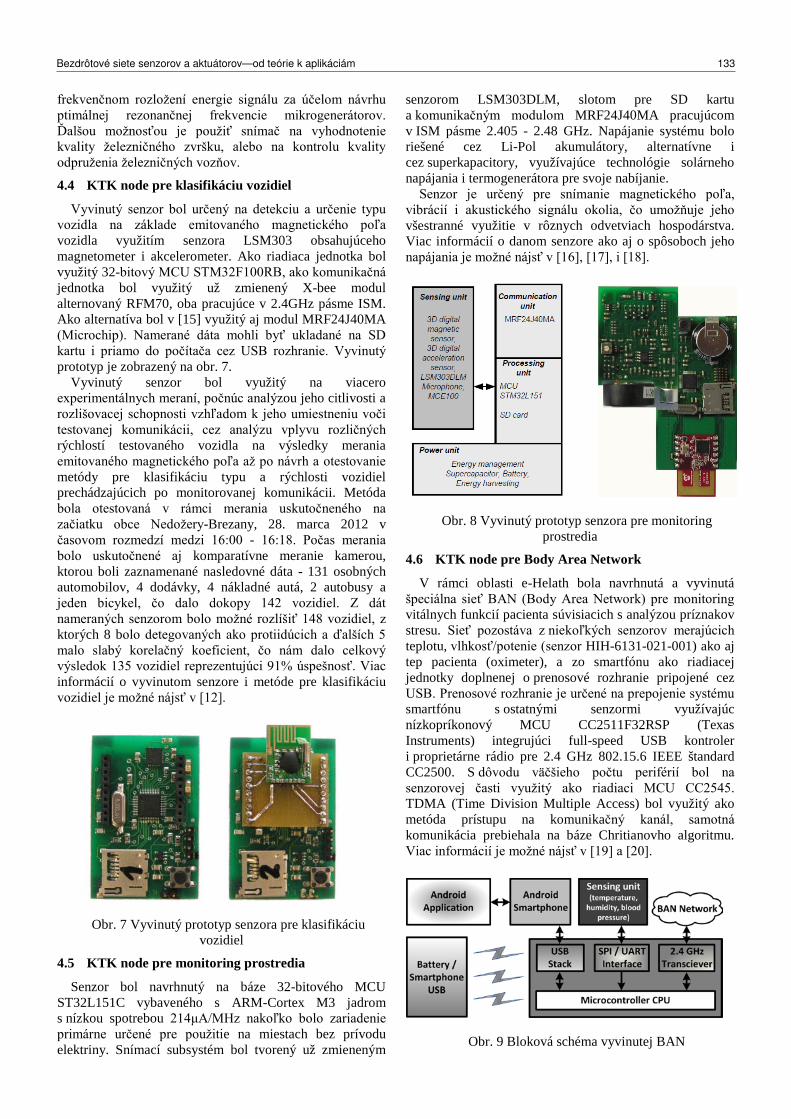
frekvenčnom rozložení energie signálu za účelom návrhu ptimálnej rezonančnej frekvencie mikrogenerátorov. Ďalšou možnosťou je použiť snímač na vyhodnotenie kvality železničného zvršku, alebo na kontrolu kvality odpruženia železničných vozňov.

4.4 KTK node pre klasifikáciu vozidiel

Vyvinutý senzor bol určený na detekciu a určenie typu vozidla na základe emitovaného magnetického poľa vozidla využitím senzora LSM303 obsahujúceho magnetometer i akcelerometer. Ako riadiaca jednotka bol využitý 32-bitový MCU STM32F100RB, ako komunikačná jednotka bol využitý už zmienený X-bee modul alternovaný RFM70, oba pracujúce v 2.4GHz pásme ISM. Ako alternatíva bol v [15] využitý aj modul MRF24J40MA (Microchip). Namerané dáta mohli byť ukladané na SD kartu i priamo do počítača cez USB rozhranie. Vyvinutý prototyp je zobrazený na obr. 7.

Vyvinutý senzor bol využitý na viacero experimentálnych meraní, počnúc analýzou jeho citlivosti a rozlišovacej schopnosti vzhľadom k jeho umiestneniu voči testovanej komunikácii, cez analýzu vplyvu rozličných rýchlostí testovaného vozidla na výsledky merania emitovaného magnetického poľa až po návrh a otestovanie metódy pre klasifikáciu typu a rýchlosti vozidiel prechádzajúcich po monitorovanej komunikácii. Metóda bola otestovaná v rámci merania uskutočneného na začiatku obce Nedožery-Brezany, 28. marca 2012 v časovom rozmedzí medzi 16:00 - 16:18. Počas merania bolo uskutočnené aj komparatívne meranie kamerou, ktorou boli zaznamenané nasledovné dáta - 131 osobných automobilov, 4 dodávky, 4 nákladné autá, 2 autobusy a jeden bicykel, čo dalo dokopy 142 vozidiel. Z dát nameraných senzorom bolo možné rozlíšiť 148 vozidiel, z ktorých 8 bolo detegovaných ako protiidúcich a ďalších 5 malo slabý korelačný koeficient, čo nám dalo celkový výsledok 135 vozidiel reprezentujúci 91% úspešnosť. Viac informácií o vyvinutom senzore i metóde pre klasifikáciu vozidiel je možné nájsť v [12].

Obr. 7 Vyvinutý prototyp senzora pre klasifikáciu vozidiel

4.5 KTK node pre monitoring prostredia

Senzor bol navrhnutý na báze 32-bitového MCU ST32L151C vybaveného s ARM-Cortex M3 jadrom s nízkou spotrebou 214μA/MHz nakoľko bolo zariadenie primárne určené pre použitie na miestach bez prívodu elektriny. Snímací subsystém bol tvorený už zmieneným

senzorom LSM303DLM, slotom pre SD kartu a komunikačným modulom MRF24J40MA pracujúcom v ISM pásme 2.405 - 2.48 GHz. Napájanie systému bolo riešené cez Li-Pol akumulátory, alternatívne i cez superkapacitory, využívajúce technológie solárneho napájania i termogenerátora pre svoje nabíjanie.

Senzor je určený pre snímanie magnetického poľa, vibrácií i akustického signálu okolia, čo umožňuje jeho všestranné využitie v rôznych odvetviach hospodárstva. Viac informácií o danom senzore ako aj o spôsoboch jeho napájania je možné nájsť v [16], [17], i [18].

Obr. 8 Vyvinutý prototyp senzora pre monitoring

prostredia

4.6 KTK node pre Body Area Network

V rámci oblasti e-Helath bola navrhnutá a vyvinutá špeciálna sieť BAN (Body Area Network) pre monitoring vitálnych funkcií pacienta súvisiacich s analýzou príznakov stresu. Sieť pozostáva z niekoľkých senzorov merajúcich teplotu, vlhkosť/potenie (senzor HIH-6131-021-001) ako aj tep pacienta (oximeter), a zo smartfónu ako riadiacej jednotky doplnenej o prenosové rozhranie pripojené cez USB. Prenosové rozhranie je určené na prepojenie systému smartfónu s ostatnými senzormi využívajúc nízkopríkonový MCU CC2511F32RSP (Texas Instruments) integrujúci full-speed USB kontroler i proprietárne rádio pre 2.4 GHz 802.15.6 IEEE štandard CC2500. S dôvodu väčšieho počtu periférií bol na senzorovej časti využitý ako riadiaci MCU CC2545. TDMA (Time Division Multiple Access) bol využitý ako metóda prístupu na komunikačný kanál, samotná komunikácia prebiehala na báze Chritianovho algoritmu. Viac informácií je možné nájsť v [19] a [20].

Obr. 9 Bloková schéma vyvinutej BAN

Bezdrôtové siete senzorov a aktuátorov—od teórie k aplikáciám 133

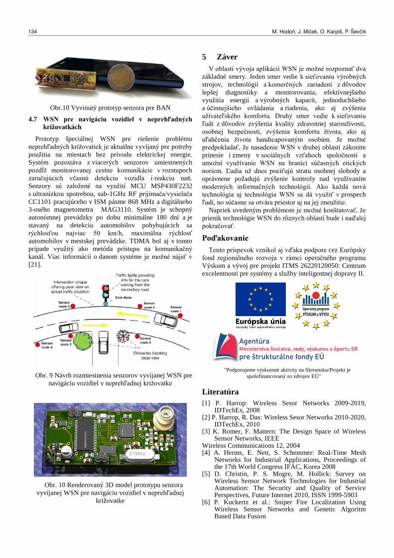
Obr.10 Vyvinutý prototyp senzora pre BAN

4.7 WSN pre navigáciu vozidiel v neprehľadných križovatkách

Prototyp špeciálnej WSN pre riešenie problému neprehľadných križovatiek je aktuálne vyvíjaný pre potreby použitia na miestach bez prívodu elektrickej energie. Systém pozostáva z viacerých senzorov umiestnených pozdĺž monitorovanej cestne komunikácie v rozstupoch zaručujúcich včasnú detekciu vozidla i reakciu naň. Senzory sú založené na využití MCU MSP430F2232 s ultranízkou spotrebou, sub-1GHz RF prijímača/vysielača CC1101 pracujúceho v ISM pásme 868 MHz a digitálneho 3-osého magnetometra MAG3110. Systém je schopný autonómnej prevádzky po dobu minimálne 180 dní a je stavaný na detekciu automobilov pohybujúcich sa rýchlosťou najviac 50 km/h, maximálna rýchlosť automobilov v mestskej prevádzke. TDMA bol aj v tomto prípade využitý ako metóda prístupu na komunikačný kanál. Viac informácií o danom systéme je možné nájsť v [21].

Obr. 9 Návrh rozmiestnenia senzorov vyvíjanej WSN pre

navigáciu vozidiel v neprehľadnej križovatke

Obr. 10 Renderovaný 3D model prototypu senzora

vyvíjanej WSN pre navigáciu vozidiel v neprehľadnej križovatke

5 Záver V oblasti vývoja aplikácií WSN je možné rozpoznať dva

základné smery. Jeden smer vedie k sieťovaniu výrobných strojov, technológií a komerčných zariadení z dôvodov lepšej diagnostiky a monitorovania, efektívnejšieho využitia energií a výrobných kapacít, jednoduchšieho a účinnejšieho ovládania a riadenia, ako aj zvýšenia užívateľského komfortu. Druhý smer vedie k sieťovaniu ľudí z dôvodov zvýšenia kvality zdravotnej starostlivosti, osobnej bezpečnosti, zvýšenia komfortu života, ako aj uľahčenia života handicapovaným osobám. Je možné predpokladať, že nasadenie WSN v druhej oblasti zákonite prinesie i zmeny v sociálnych vzťahoch spoločnosti a umožní využívanie WSN na hranici súčasných etických noriem. Ľudia už dnes pociťujú stratu osobnej slobody a oprávnene požadujú zvýšenie kontroly nad využívaním moderných informačných technológií. Ako každá nová technológia aj technológia WSN sa dá využiť v prospech ľudí, no súčasne sa otvára priestor aj na jej zneužitie.

Napriek uvedeným problémom je možné konštatovať, že prienik technológie WSN do rôznych oblastí bude i naďalej pokračovať.

Poďakovanie Tento príspevok vznikol aj vďaka podpore cez Európsky

fond regionálneho rozvoja v rámci operačného programu Výskum a vývoj pre projekt ITMS 26220120050: Centrum excelentnosti pre systémy a služby inteligentnej dopravy II.

"Podporujeme výskumné aktivity na Slovensku/Projekt je

spolufinancovaný zo zdrojov EÚ"

Literatúra [1] P. Harrop: Wireless Sesor Networks 2009-2019,

IDTechEx, 2008 [2] P. Harrop, R. Das: Wireless Sesor Networks 2010-2020,

IDTechEx, 2010 [3] K. Romer, F. Mattern: The Design Space of Wireless

Sensor Networks, IEEE Wireless Communications 12, 2004 [4] A. Herms, E. Nett, S. Schemmer: Real-Time Mesh

Networks for Industrial Applications, Proceedings of the 17th World Congress IFAC, Korea 2008

[5] D. Christin, P. S. Mogre, M. Hollick: Survey on Wireless Sensor Network Technologies for Industrial Automation: The Security and Quality of Service Perspectives, Future Internet 2010, ISSN 1999-5903

[6] P. Kuckertz et al.: Sniper Fire Localization Using Wireless Sensor Networks and Genetic Algoritm Based Data Fusion

134 M. Hodon, J. Micek, O. Karpiš, P. Ševcík

[7] H. M. F. AboEiFotoh, E. S. ElMallah, H. S. Hassanin: On The Reliability of Wireless Sensor Networks, IEEE ICC, 2006

[8] M. Cinque, D. Controneo, G. De Caro, M. Pelella: Reliability Requirements of Wireless Sensor Networks for Dynamic Structural Monitoring, Proceedings of Workshop on Applied Software Reliability, Philadelphia, USA 2006

[9] J. Miček: Bezdrôtové senzorické siete-súčasnosť, perspektívy, aplikácie, ATP Journal, 7, 8, 9, 10, 2011, ISSN 1335-2237

[10] P. Dutta, et al.: A Building Block Approach to Sensornet Systems, In Proc. SenSys 08, 2008, North Carolina, USA.

[11] O. Karpiš, J. Miček: Sniper localization using WSN 2011. In: ICMT´11. - Brno : University of Defence, 2011. - ISBN 9788072317875. - S. 1063-1068.

[12] O. Karpiš: Sensor for Vehicles Classification. In Proceedings of the Federated Conference on Computer Science and Information Systems pp. 785–789, ISBN 978-83-60810-51-4.

[13] J. Miček, J. Kapitulík: Wireless sensors networks in road transportation applications. IEEE Perspective Technologies and Methods in MEMS Design (MEMSTECH), 11-14 May 2011, Lviv, Ukraine.

[14] J. Papán, M. Jurečka a J. Púchyová: WSN for Forest Monitoring to Prevent Illegal Logging. Proceedings of the Federated Conference on Computer Science and Information Systems pp. 809–812, ISBN 978-83-60810-51-4.

[15] O. Karpiš: Solar-cell based powering of a node for traffic monitoring IOSR Journal of Engineering, Vol. 3, Issue 4 (April. 2013), pp. 28-32 ), e-ISSN: 2250-3021, p-ISSN: 2278-8719.

[16] J. Miček, J. Kapitulík: WSN sensor node for protected area monitoring. Proceedings of the Federated Conference on Computer Science and Information Systems pp. 803–807, ISBN 978-83-60810-51-4.

[17] J. Miček, J. Kapitulík: Wireless Sensor Node for Traffic Monitoring: Analysis and Design. European International Journal of Science and Technology, Vol. 2, No. 1, February 2013, pp.85-97, ISSN: 2304-9693

[18] M. Kochláň, P. Ševčík: Supercapacitor power unit for an event-driven wireless sensor node. Proceedings of the Federated Conference on Computer Science and Information Systems pp. 791–796, ISBN 978-83-60810-51-4

[19] M. Kochláň, M. Hodoň, J. Púchyová: Vital functions monitoring via Sensor Body Area Network with smartphone network coordinator. In: MEMSTECH´ 2013, 16-20 April 2013, Polyana, Ukraine, pp.143-147, ISBN 978-617-607-424-3.

[20] M. Hodoň, J. Púchyová, M. Kochláň: Smartphone-Based Body Area Network for Stress Monitoring: Radio Interference Investigation. Communications: scientific letters of the University of Žilina, ISSN 1335-4205, v tlači.

[21] M. Hodoň, J. Miček, M. Chovanec: Wireless Sensor Networks for Intelligent Transportation Systems. IEEE CommSoft newsletter: No. 2, 2012, v tlači.

Bezdrôtové siete senzorov a aktuátorov—od teórie k aplikáciám 135

Index

Andel, M., 48

Bajer L., 86Benítez, M., 63Brázdová, M., 42Brejová, B., 35, 47, 69Brunetto, R., 111Budiš, J., 35

Cegan, R., 63Charypar, V., 86

Didi, V., 63Dobisová, T., 63Duriš, M., 120

Gloser, V., 63

Hajic jr., J., 5Hejátko, J., 62, 63Hlavácová, J., 2Hobza, R., 63Hodon, M., 128Holena, M., 77, 86, 92, 104Horváth, T., 21Hrdinová, V., 62Hubata-Vacek, V., 100

Ihnátová, I., 56

Janda, L., 62

Karpiš, O., 128Katerniaková, J., 120Kléma, J., 48Klumpler, T., 62Kopp, M., 92Krejcík, Z., 48Kubátová, H., 121Kurková, V., 73

Lexa, M., 42, 64Lupták, A., 47

Martínek, T., 42Micek, J., 128

Nguyen, T., 27

Ostertág, R., 122, 125

Peška, L., 22Pejla, J., 104Pekárová, B., 62Pero, Š., 15, 21, 27

Rampášek, L., 47Richta, K., 121Richta, T., 121

Šcavnický, M., 77Ševcík, P., 128Šimal’ová, M., 36Štefanic, S., 64

Veselovská, K., 5Vinar, T., 47, 69Vojír, S., 10

136