University of Kentucky University of Kentucky

UKnowledge UKnowledge

University of Kentucky Master's Theses Graduate School

2004

TOLERANCE ALLOCATION FOR KINEMATIC SYSTEMS TOLERANCE ALLOCATION FOR KINEMATIC SYSTEMS

Mathieu Barraja University of Kentucky, mbarr0@engr.uky.edu

Right click to open a feedback form in a new tab to let us know how this document benefits you. Right click to open a feedback form in a new tab to let us know how this document benefits you.

Recommended Citation Recommended Citation Barraja, Mathieu, "TOLERANCE ALLOCATION FOR KINEMATIC SYSTEMS" (2004). University of Kentucky Master's Theses. 315. https://uknowledge.uky.edu/gradschool_theses/315

This Thesis is brought to you for free and open access by the Graduate School at UKnowledge. It has been accepted for inclusion in University of Kentucky Master's Theses by an authorized administrator of UKnowledge. For more information, please contact UKnowledge@lsv.uky.edu.

ABSTRACT OF THESIS

TOLERANCE ALLOCATION FOR KINEMATIC SYSTEMS

A method for allocating tolerances to exactly constrained assemblies is

developed. The procedure is established as an optimization subject to constraints. The objective is to minimize the manufacturing cost of the assembly while respecting an acceptable level of performance. This method is particularly interesting for exactly constrained components that should be mass-produced.

This thesis presents the different concepts used to develop the method. It describes exact constraint theory, manufacturing variations, optimization concepts, and the related mathematical tools. Then it explains how to relate these different topics in order to perform a tolerance allocation.

The developed method is applied on two relevant exactly constrained examples: multi-fiber connectors, and kinematic coupling. Every time a mathematical model of the system and its corresponding manufacturing variations is established. Then an optimization procedure uses this model to minimize the manufacturing cost of the system while respecting its functional requirements. The results of the tolerance allocation are verified with Monte Carlo simulation.

KEYWORDS: Tolerance Allocation, Manufacturing Variation, Kinematic Design Theory, Optimization

Mathieu Barraja

September 9, 2002

Copyright © Mathieu Barraja 2002.

TOLERANCE ALLOCATION FOR KINEMATIC SYSTEMS

By

Mathieu Barraja

Prof. R. Ryan Vallance, PhD

Director of Thesis

Dr. George Huang, PhD

Director of Graduate Studies

Copyright © Mathieu Barraja 2002.

RULES FOR THE USE OF THESES

Unpublished theses submitted for the Master’s degree and deposited in the University of Kentucky Library are a rule open for inspection, but are to be used only with due regard to the rights of the authors. Bibliographical references may be noted, but quotations or summaries of parts may be published only with the permission of the author, and with the usual scholarly acknowledgements. Extensive copying or publication of the theses in whole or in part also requires the consent of the Dean of the Graduate School of the University of Kentucky.

THESIS

Mathieu Barraja

The Graduate School

University of Kentucky

2002

TOLERANCE ALLOCATION FOR KINEMATIC SYSTEMS

THESIS

A thesis submitted in partial fulfillment of the requirements for the degree of MSME in the

College of Engineering at the University of Kentucky

By

Mathieu Barraja

Lexington, Kentucky

Director: Dr. R.R. Vallance, Assistant Professor of Mechanical Engineering Department

Lexington, Kentucky

2002

iii

ACKNOWLEDGEMENTS

First of all I would like to thank Mr. Georges Verchery and Mr. Shahram

Aivazzadeh for giving me the opportunity to enter a Master’s degree program at the

University of Kentucky. I hope they consider this very first UK thesis written by an

isatian as the result of their hard work for establishing an academic partnership between

UK and ISAT Nevers. For the same reason, I would like to thank Dr. G.T. Lineberry

who accepted my application for the University of Kentucky. And I can’t forget Miss

Christine Gonzalez, who could overcome all the administrative difficulties that were

swarming in my application file.

Next, I would like to express my deepest gratitude to my advisor, Dr. R. Ryan

Vallance. I fully realize that my experience in UK would not have been so enriching if I

hadn’t met him. I cannot imagine an advisor more dedicated to his students and more

thoughtful to their researches. I admire him for his outstanding engineering knowledge,

but also for his great human qualities.

I am also really thankful towards people in TCS for having given me the

opportunity to work on an exciting project. I would like to thank John Lehman, Burke

Hunsaker, and especially Dr. Sepehr Kiani. They’ve always supported my research, and

I hope the result of my work can be equal to the gratitude I would like to show them. I

have learnt a lot from them.

Finally, I would like to thank Dr. Stephens and Dr. Mengüç as my examining

committees. I wish the results of my project might find some application in their

researches; knowing that they would find such an interest in my works would be a

personal reward.

iv

TABLE OF CONTENTS

ACKNOWLEDGEMENTS................................................................................................................... iii

LIST OF TABLES................................................................................................................................ vii

LIST OF FIGURES............................................................................................................................. viii

LIST OF FILES...................................................................................................................................... x

CHAPTER 1: INTRODUCTION AND THESIS OVERVIEW...................................................... 1

1.1. BACKGROUND TO THE THESIS ........................................................................................................ 1 1.2. PRIOR WORK AND LITERATURE REVIEW......................................................................................... 2

1.2.1. Exactly Constrained Systems.............................................................................................. 2 1.2.2. Dimensional Variations ..................................................................................................... 3 1.2.3. Least Cost Tolerance Allocation......................................................................................... 4 1.2.4. Mathematics and Statistics................................................................................................. 4

1.3. THESIS OVERVIEW ......................................................................................................................... 5 1.3.1. Hypothesis......................................................................................................................... 5 1.3.2. Content Overview .............................................................................................................. 5

CHAPTER 2: CONCEPTS USED IN THE METHOD .................................................................. 6

2.1. EXACTLY CONSTRAINED SYSTEMS ................................................................................................. 6 2.1.1. Theory ............................................................................................................................... 6 2.1.2. Types of Connection........................................................................................................... 7 2.1.3. Example of Kinematic Spindle.......................................................................................... 10

2.2. MANUFACTURING VARIATIONS .................................................................................................... 14 2.2.1. Presentation .................................................................................................................... 14

2.2.1.1. Introduction ............................................................................................................. 14 2.2.1.2. Sources of Variations ............................................................................................... 15

2.2.2. Mathematical Representation........................................................................................... 16 2.2.2.1. Dimensions as Random Variables............................................................................. 16 2.2.2.2. Mathematical Model of the Geometric Specifications................................................ 17

2.2.3. Methods to Analyze the Variations ................................................................................... 19 2.2.3.1. Monte Carlo Simulation ........................................................................................... 19 2.2.3.2. Analytical Model...................................................................................................... 20 2.2.3.3. Multivariate Error Analysis ...................................................................................... 21 2.2.3.4. Comparison of the Methods...................................................................................... 22

2.3. LEAST COST TOLERANCE ALLOCATION ........................................................................................ 23 2.3.1. Introduction..................................................................................................................... 23 2.3.2. Tolerance Allocation by Optimization .............................................................................. 24 2.3.3. Cost / Tolerance Relations ............................................................................................... 25

2.4. CHAPTER SUMMARY .................................................................................................................... 27

CHAPTER 3: APPLICATION TO OPTICAL FIBER CONNECTORS..................................... 30

3.1. INTRODUCTION ............................................................................................................................ 30 3.1.1. Presentation .................................................................................................................... 30

3.1.1.1. Fiber Optics ............................................................................................................. 30 3.1.1.2. Transmission Losses................................................................................................. 31 3.1.1.3. Optical Fiber Connectors.......................................................................................... 33

3.1.2. Background and Prior Work ............................................................................................ 34 3.1.3. Tolerance Allocation........................................................................................................ 35

3.2. MATHEMATICAL MODEL.............................................................................................................. 38 3.2.1. Exact Constraints Within the Connector........................................................................... 38

v

3.2.2. Parametric Model of the Components in the Connector .................................................... 40 3.2.2.1. Presentation ............................................................................................................. 40 3.2.2.2. Pins and Fiber Claddings .......................................................................................... 42 3.2.2.3. Cores of Fibers......................................................................................................... 43 3.2.2.4. Ferrules.................................................................................................................... 44 3.2.2.5. List of the Variables ................................................................................................. 45

3.2.3. Mathematic Description of the Geometric Model.............................................................. 46 3.2.3.1. Assembly of a Random Cylinder Inside a Random Vee-Groove ................................ 46 3.2.3.2. Creating an Array of Fibers ...................................................................................... 50 3.2.3.3. Mating Two Fibers................................................................................................... 53

3.3. TOLERANCE ALLOCATION ............................................................................................................ 55 3.3.1. Overview ......................................................................................................................... 55 3.3.2. Variation Analysis by the Law of Error Propagation ........................................................ 56 3.3.3. Cost / Tolerance Functions .............................................................................................. 60 3.3.4. Results of the Tolerance Allocation Algorithm.................................................................. 61 3.3.5. Comparison with Monte Carlo Simulation........................................................................ 63

3.4. MANUFACTURING PROCESS.......................................................................................................... 64 3.4.1. Introduction..................................................................................................................... 64 3.4.2. Description of the Process ............................................................................................... 65 3.4.3. Metallography Study........................................................................................................ 66 3.4.4. Stylus Profilometry of Grooves......................................................................................... 68 3.4.5. Conclusions ..................................................................................................................... 71

CHAPTER 4: APPLICATION TO KINEMATIC COUPLINGS ................................................ 72

4.1. INTRODUCTION ............................................................................................................................ 72 4.1.1. Presentation .................................................................................................................... 72 4.1.2. Background and Prior Work ............................................................................................ 73 4.1.3. Tolerance Allocation........................................................................................................ 75

4.2. MATHEMATICAL MODEL.............................................................................................................. 78 4.2.1. Parametric Representation of Contacting Surfaces........................................................... 78 4.2.2. Resting Position and Orientation...................................................................................... 80 4.2.3. Multivariate Error Analysis of Variation in Resting Location ........................................... 83 4.2.4. Variation at Operating Points .......................................................................................... 85

4.3. TOLERANCE ALLOCATION ............................................................................................................ 88 4.3.1. Manufacturing Cost and Tolerances................................................................................. 88 4.3.2. Tolerance Allocation by Optimization .............................................................................. 90 4.3.3. Verification by Monte Carlo Simulation ........................................................................... 94

4.4. CONCLUSION ............................................................................................................................... 95

CHAPTER 5: CONCLUSIONS AND FUTURE WORK ............................................................. 96

5.1. CONCLUSIONS ............................................................................................................................. 96 5.2. FUTURE WORK ............................................................................................................................ 96

APPENDIX A:...................................................................................................................................... 98

PROBABILITY DENSITY FUNCTION OF SUM OF SQUARES .................................................... 98

APPENDIX B: .................................................................................................................................... 101

MATLAB CODES FOR KINEMATIC COUPLINGS...................................................................... 101

B1. OPTIMIZATION: OBJECTIVE FUNCTION............................................................................................. 101 B2. OPTIMIZATION: CONSTRAINT FUNCTIONS ........................................................................................ 103 B3. OPTIMIZATION: INVOKING FILE ....................................................................................................... 104 B4. MONTE CARLO SIMULATION ........................................................................................................... 105 B5. SUB-FUNCTION: KCT_BALLGEOM .................................................................................................... 107 B6. SUB-FUNCTION: KCT_CENTROID...................................................................................................... 109

vi

B7. SUB-FUNCTION: KCT_ERRORS.......................................................................................................... 111 B8. SUB-FUNCTION: KCT_GROOVEGEOM ............................................................................................... 115 B9. SUB-FUNCTION: KCT_PERTURB ....................................................................................................... 118 B10. SUB-FUNCTION: KCT_REST............................................................................................................ 122 B11. SUB-FUNCTION: KCT_SEAT ........................................................................................................... 125

APPENDIX C:.................................................................................................................................... 128

DETERMINING THE HTM FROM A METROLOGY DATUM FRAME TO A CENTROIDAL COORDINATE SYSTEM.................................................................................................................. 128

REFERENCES................................................................................................................................... 133

VITA .................................................................................................................................140

vii

List of Tables Table 2-1: 3D Symbols of Connections for Kinematic Diagrams (after ISO 3952-1) .......8 Table 2-2: Comparison of Methods for Analyzing System Variability ...........................23 Table 3-1: Variables Used in the 2D Parametric Model of the Connector ......................46 Table 3-2: Computed Tolerances for Exemplary Connector...........................................62 Table 3-3: Statistics of 2D Geometric Parameters Describing Vee-Groove Variation.....71 Table 4-1: Coefficients for Cost / Tolerance Relations...................................................89 Table 4-2: Constraints Used for Exemplary Tolerance Allocation..................................93 Table 4-3: Computed Tolerances ...................................................................................93 Table 4-4: Comparison Optimization / Simulation.........................................................95

viii

List of Figures Fig 2-1: Kinematic Analysis of the Concept of a Spindle...............................................10 Fig 2-2: Kinematic Analysis of the First Possible Architecture for the Spindle ..............11 Fig 2-3: Kinematic Analysis of the Second Possible Architecture for the Spindle ..........11 Fig 2-4: Kinematic Diagrams of Equivalent Contacts ....................................................12 Fig 2-5: Mapping of the Contacts in the Final Design of the Exactly Constrained Spindle

...............................................................................................................................12 Fig 2-6: Kinematic Diagram of the Final Design of the Exactly Constrained Spindle.....13 Fig 2-7: Exactly Constrained Spindle Corresponding to the Presented Kinematic Analysis

...............................................................................................................................14 Fig 2-8: Flatness Specifications Transformed into Dimensional Tolerances...................18 Fig 2-9: Flowchart of Least Cost Tolerance Allocation for Kinematic System ...............29 Fig 3-1: Structure of an Optical Fiber ............................................................................30 Fig 3-2: Misalignments Generating Connection Losses Between Mating Fibers ............33 Fig 3-3: Optical Fiber Connector with Kinematically Designed Ferrules .......................34 Fig 3-4: Flowchart of the Tolerance Allocation for Optical Fiber Connector..................37 Fig 3-5: Kinematic Analysis of the Exactly Constrained Connector ...............................38 Fig 3-6: 3D Kinematic Diagram of the Exactly Constrained Connector .........................39 Fig 3-7: Male Ferrule in the xy-Plane.............................................................................39 Fig 3-8: 2D Model of a Perfect Fiber and a Real Fiber...................................................40 Fig 3-9: 2D Model of a Perfect Array of Fibers .............................................................41 Fig 3-10: 2D Model of an Array of Fibers with Manufacturing Variations.....................41 Fig 3-11: 2D Model of Mating Arrays of Fibers with Manufacturing Variations............42 Fig 3-12: Different Possible Errors in a Cylindrical Feature...........................................43 Fig 3-13: 2D Parametric Representation of a Ferrule .....................................................44 Fig 3-14: Location of a Random Cylinder in a Random Vee-Groove .............................47 Fig 3-15: Shape of a Random Ferrule in 2D...................................................................51 Fig 3-16: Experimental Determination of a Relation......................................................54 Fig 3-17: Outputs of Monte Carlo Simulation................................................................59 Fig 3-18: Computed Losses for Optimized Exemplary Connector..................................62 Fig 3-19: Flowchart of Monte Carlo Simulation for Multi-Fiber Connectors..................63 Fig 3-20: Monte Carlo Simulation for Exemplary Connector with Optimized Tolerances

...............................................................................................................................64 Fig 3-21: SEM Image of Micro Vee-grooves Following Wired EDM Operation............66 Fig 3-22: Metallography Study of a Vee-Groove Produced with Wire EDM..................67 Fig 3-23: Metallographic Study of Coated Vee-Groove .................................................68 Fig 3-24: Point Cloud from Profilometry Traces............................................................69 Fig 3-25: 3D Profilometry Data Projected onto a 2D Plane for Comparison to Ideal

Model .....................................................................................................................69 Fig 3-26: Manufacturing Errors in a Vee-Groove...........................................................70 Fig 4-1: Three-Groove Kinematic Coupling ..................................................................72 Fig 4-2: Flowchart of the Tolerance Allocation for Kinematic Couplings ......................77 Fig 4-3: Parametric Representation of Spherical and Flat Contacting Surfaces...............78 Fig 4-4: Solution for Resting Position and Orientation...................................................81

ix

Fig 4-5: Vector Loop Between Ball and Flat Surface .....................................................83 Fig 4-6: Coupled Kinematic Coupling with Operating Point ..........................................86 Fig 4-7: Cost / Tolerance Relations for Dimensions.......................................................90 Fig 4-8: Dimension Schemes for the Ball Pallet, in its Datum Frame .............................92 Fig 4-9: Dimension Schemes for the Groove Body, in its Datum Frame ........................92 Fig 4-10: Flowchart of Monte Carlo Simulation for Kinematic Couplings .....................94

x

List of Files

Mbarraja.pdf…………………………………………………………………….1,497 KB

1

Chapter 1: Introduction and Thesis Overview

1.1. Background to the Thesis

Kinematic design is widely used in precision engineering. In effect, kinematic

systems, also known as exactly constrained systems, present good repeatability if

stiffness and load capacity are not critical parameters [1]. Moreover, the behavior of

kinematic systems can be described in a mathematical model, since the location of the

exact constraints are analytically defined by one unique solution [2]. It is then possible to

develop an analytical tool that can help the designer of a kinematic system to make an

optimized design [3].

On the other hand, kinematic design provides economical solutions for making

repeatable assemblies. In effect, the design of kinematic systems is often relatively

simple, and they can be easily manufactured. These good characteristics make the

kinematic systems interesting for mass production, where they can be used in

manufacturing, fixturing, and material handling. For instance, Vallance and Slocum [4]

described the use of kinematic couplings for positioning pallets in flexible assembly

systems.

However, a poor tolerance allocation may affect the precision of a kinematic

system, despite its good repeatability. This is a major problem if the kinematic systems

are intended for interchangeable assemblies, for instance a fixturing feature that is used

on several workstations of a production line. Hence an efficient tolerance allocation is of

primary interest for exactly constrained systems.

Teradyne Connection Systems (TCS), a manufacturer of daughtercard and

backplane connectors, is developing a multifiber optical connector by following the

kinematic design principles. This connector will be manufactured in mass production, so

TCS wants to allocate the tolerances on this product so that its manufacturing cost is

minimized while its required accuracy is preserved. Furthermore, the Precision Systems

Laboratory of the University of Kentucky is conducting an extensive study on kinematic

couplings; a tolerance allocation on these exactly constrained features could contribute to

this wide analysis.

2

These two requirements have led to the development of a general approach for

allocating tolerances on kinematic systems. This thesis is the result of this work. It

describes the method in detail, with the different engineering principles used. Then the

tolerance allocation is applied to the multifiber optical connector and the kinematic

coupling for illustrating the developed method.

1.2. Prior Work and Literature Review

This section introduces the main principles of mechanics and mathematics with

the corresponding relevant literature reviews that will serve as the background to the

work done in this thesis. The materials covered are the exactly constrained systems, the

dimensional variations of a manufactured part, and tolerance allocation using least cost

optimization.

1.2.1. Exactly Constrained Systems

The principle of kinematic design states that point contact should be established at

the minimum number of points required to constrain a body in the desired position and

orientation [1]. In this case, the degrees of freedom of the rigid system are exactly

constrained, so a mathematical model of the system can exactly predict its location. Prior

studies used this property to develop analytical methods for designing kinematic systems.

One of the best examples is given by Schmiechen and Slocum [3], who published

a design method using linear algebra to represent the geometry of a kinematic assembly.

They could derive a simple expression for determining the error motions within the

assembly in function of the applied forces. They could also quantify the stability of the

kinematic system. This publication demonstrates that an analytical model of a kinematic

system is a powerful tool for improving its design. A similar approach can be used to

develop a variation study of the exactly constrained system.

Blanding [5] made an extensive study of the theoretical aspect of kinematic

design. On a more practical point of view, the standard ISO 3952-1 [6] presents a

convenient way to represent symbolically the kinematic links of a mechanical system,

3

and it is a powerful tool for the designer to determine whether a system is exactly

constrained or not.

1.2.2. Dimensional Variations

Manufacturing perfect dimensions is impossible. In effect, it is well known that

any manufacturing process is subject to variations, and the produced parts can’t have

exactly the same dimensions. Furthermore, the dimensions may change with time or

environmental conditions, which can for instance generate wear or thermal expansion.

This is the reason why a designer has to affect tolerances to the nominal dimensions, in

order to specify the acceptable limits of the variations. The functionality of a part should

be accepted if its dimensions stay within their assigned tolerances.

Tolerances can be either dimensional or geometric. If they are dimensional, they

define the acceptable range of values that a length or an angle can get. If they are

geometric, they put conditions on the shape of the part, such as flatness, roundness or

angularity. Standards [7,8] cover this subject in detail and provide to the designer useful

recommendations for assigning efficiently the tolerances.

Manufactured dimensions are hence subject to variations. It is then possible to

express them as randomly distributed variables to analyze them through a mathematical

model. Actually, the Statistical Process Control (SPC) method, widely used in industry

for quality insurance, is based on this concept [9].

A thorough analysis of the geometry of a kinematic system should take into

consideration these dimensional variations. The mathematical model of the system will

set up the nominal value and the tolerances of the dimensions in terms of expected value

and standard deviation of the corresponding random variables. The variation analysis of

the kinematic coupling will then be based upon concepts from statistics.

4

1.2.3. Least Cost Tolerance Allocation

Chase [10] presented several relevant techniques for allocating tolerances on

mechanical systems. The most efficient one is arguably the tolerance allocation using

least cost optimization.

Studies have experimentally determined relations between cost and tolerance for

different manufacturing processes since the 1940s [11]. Linear regressions of the

measured data provide empirical functions describing these relations. By combining

these functions to the mathematical model of the analyzed kinematic system, it is possible

to determine the manufacturing cost of the system for a given accuracy.

Such a mathematical model can be implemented in a tolerance allocation routine.

By using an optimization technique, the designer can assign the tolerances such that the

manufacturing cost of the system is minimized while its functional requirements are

respected. The tolerance allocation is then formulated as a minimization subject to

constraints.

Some mathematical software packages include an optimization toolbox [12]. It is

a convenient tool for solving optimization problems with multiple parameters, which can

be faced in any discipline. The user has to implement the problem in an algorithm, by

defining the objective and the constraints in a mathematical form.

If it is decided to optimize the design of a kinematic system by least cost tolerance

allocation, the objective function is the manufacturing cost of the parts, which has to be

minimized. The constraints are the mathematical expressions of the functional

requirements of the product, which are generally directly related to the accuracy of the

system.

1.2.4. Mathematics and Statistics

This thesis presents overall an analytical work, so it relies heavily on several

topics from mathematics and statistics. Mathematical models of the exactly constrained

systems are based on analytic geometry [13]. One of the methods for analyzing the

variations of the system calls for homogeneous transformation matrices [1,14], then a

5

multivariate error analysis [15] is performed. A completely analytical model of the

systems, which combines continuous random variables in non-linear relations, is another

alternative for evaluating the location and orientation variations of a system; hence a

reliable reference in engineering statistics is required [16]. In several cases, the methods

resort to regression analyses [16] for fitting the experimental data. Finally, random

simulations using the Monte Carlo method [17] are extensively used for estimating the

statistics of the output parameters.

1.3. Thesis Overview

This thesis describes a method for allocating tolerances on kinematic systems.

The objective is to find virtually the best combination of tolerances to set on an exactly

constrained assembly in order to reduce its manufacturing cost related to its geometric

and dimensional variations, while its functional requirement is respected.

1.3.1. Hypothesis

Prior work reviews show that a thorough analysis of kinematic systems can

predict with accuracy their mechanical behavior [3,18]. On the other hand, there exist

many methods for assigning tolerances to mechanical assemblies [19], with different

levels of efficiency. Hence the hypothesis stipulates that it is possible to define a

tolerance allocation method made especially for kinematic systems. Since this method

would be based on exact analytical models, it should be better than the current tolerance

allocations available for mechanical assemblies in general.

1.3.2. Content Overview

Chapter 2 describes the different concepts used in the method. It covers

kinematic design theory, the manufacturing variations, and the principles of least cost

tolerance allocation, with the corresponding mathematical tools. The developed method

is applied to kinematically designed optical fiber connectors in Chapter 3. Then Chapter

4 presents the tolerance allocation procedure applied to kinematic couplings. Finally,

Chapter 5 discusses future work and thesis conclusions.

6

Chapter 2: Concepts Used in the Method

2.1. Exactly Constrained Systems

2.1.1. Theory

Any motion of a free rigid body in a 3D space can be described as a combination

of three pure translations and three rotations. Each of these six motion parameters is

called a degree of freedom. They can be quantitatively described if a reference frame is

attached to the space. In two dimensions, position and orientation of a free object are

only defined by two translations and one rotation.

A body is constrained if at least one of its degrees of freedom is suppressed. A

mechanical connection between two bodies suppresses one or more of their degrees of

freedom. In a mechanical assembly, the degrees of freedom to be suppressed are defined

by the functional requirements of the system. Robustness of the design of a mechanism

is improved if only the degrees of freedom that need to be removed are constrained; if a

motion can stay free, it is better not to constrain it.

Kinematic design theory [5] stipulates that a body is exactly constrained when

every degree of freedom that has to be suppressed is blocked by one single constraint. If

two or more constraints are suppressing the same degree of freedom, the system is over-

constrained. In this case, position and orientation of the body is established by several

conflicting references. Due to manufacturing variations and other sources of errors, these

references cannot match perfectly. Consequently, an over-constrained body may not fit

correctly in its assembly. If the dimensions are too loose, there will be an excessive

clearance in the assembly that may affect the functionality of the mechanism; if they are

too tight, the over-constrained body may satisfy the redundant constraints by enduring an

elastic or plastic deformation that generates internal stress within the body. In both cases,

repeatability of the assembly is affected.

Kinematic design offers some important advantages for precision engineering.

Since every suppressed degree of freedom is restricted by one single constraint, there

only exists one solution for determining the position and orientation of the constrained

body. This property provides a good repeatability to the exactly constrained mechanism,

7

if the external conditions stay relatively constant. Kinematically designed assemblies can

be manufactured at low cost, since their design is relatively simple and they don’t need

relatively tight tolerances to reach a good repeatability, compared to over-constrained

mechanisms. Moreover, location of the exactly constrained body can be predicted by

establishing a mathematical model of the assembly; there exists a straightforward

correspondence between exact constraint and exact mathematical solution. The presented

tolerance allocation method relies upon this characteristic.

However, kinematic design may not be a suitable solution for applications where

mechanical loads are important. In effect, exact constraint design tends to minimize the

area of the contacting surfaces, and then it increases tremendously the contact stress.

Another design philosophy may be used to prevent these problems: elastic averaging

intentionally over-constrains the bodies in order to carry larger loads [1]. Contact

between parts is spread on broad surfaces, so contact pressure is reduced and stiffness of

the system is increased. Manufacturing errors are averaged out, which may improve

accuracy of the assembly, but tolerances have to be tight to obtain a good level of

repeatability, which significantly increases the manufacturing cost of the system.

Exact constraint theory is therefore an adequate design tool for precision

engineering when mechanical loads are not a critical parameter. Kinematic design

provides a good repeatability at a relatively low cost.

The ideal scheme of exact constraints would be to suppress every degree of

freedom by a punctual contact. However, practical considerations, like manufacturability

of the parts or stiffness of the assembly, may prevent this theoretical scheme. Exact

constraint theory is then completed by the definition of connections, which are the

different possible combinations of constraints suppressing a set of degrees of freedom.

2.1.2. Types of Connection

When two bodies are mechanically connected, some of their degrees of freedom

are constrained. The nature of their connection is defined by determining which motions

are suppressed. An ISO standard [6] extensively describes the different types of

connections, as presented in Table 2-1.

8

Table 2-1: 3D Symbols of Connections for Kinematic Diagrams (after ISO 3952-1)

Type of Connection

Symbol Relative Motions

Possible Examples

Fixed x

yz

0 Rotation 0 Translation

Bolted assemblies; Welded parts

Pin x

y

z

1 Rotation (x) 0 Translation

Spindle in its housing; Rotating wheel on fixed

axis

Sliding x

yz

0 Rotation 1 Translation (x)

Translation stage

Helical x

yz

1 Rotation (x) 1 Translation (x)

(correlated)

Screw in tapped hole

Cylindrical x

y

z

1 Rotation (x) 1 Translation (x)

Cylinder in vee-groove

Joint x

yz

2 Rotations (x,z) 0 Translation

Universal joint

Spherical x

yz

3 Rotations 0 Translation

Sphere in cone

Planar x

yz

1 Rotation (z) 2 Translations (x,y)

Flat surface on flat surface

Ring x

yz

3 Rotations 1 Translation (x)

Sphere in vee-groove

Linear x

y

z

2 Rotations (x,z) 2 Translations (x,y)

Cylinder on flat surface

Punctual x

y

z

3 Rotations 2 Translations

Sphere on flat surface; Cylinder on

perpendicular cylinder

9

Every elementary connection may be symbolically represented by a kinematic

diagram. There exists a design procedure based upon these diagrams. By drawing the

entire kinematic diagram of the mechanism, the designer can efficiently prevent

redundant constraint and establish an exactly constrained system. This procedure starts

by mapping the constraints between the different components. It consists in enumerating

every part of the assembly, then identifying which degrees of freedom are suppressed by

the connections in every pair of interacting parts. Creating a reference coordinate system

is generally useful for determining the connections and preventing the redundant

constraints. Afterwards the designer can draw the kinematic diagram of the assembly by

representing the different connections with the corresponding symbol. It is also

important to notice that a combination of elementary connections can constrain another

degree of freedom that was not suppressed by the present elementary connections. For

clarity, a figure separated from the overall kinematic diagram of the whole assembly can

explain what the combination stands for; this is similar to a detailed view in an

engineering drawing.

Kinematic diagrams may appear at different levels of the design. First of all, they

can be used for modeling the core concept of the mechanism. At this point, the kinematic

diagram should be the simplest one and does not necessarily represent all the components

of the assembly. Basically, this first kinematic diagram should answer the question:

“What is this mechanism for?” There should be only one kinematic diagram possible for

representing the core concept of the system.

After defining the core concept of the mechanism, the following question is “How

does it work?” New kinematic diagrams can then be established for representing the

architecture of the system. Compared to the previous ones, these diagrams are more

detailed and describe the connections between the interacting parts of the assembly. At

this level, the designer can establish different diagrams, each of them illustrating a

different type of possible architecture. Once a set of potential solutions is established,

further engineering analyses will help to select the best architecture with respect to the

functionality of the mechanism. Contrarily to the diagram corresponding to the core

concept, which should be simple and fixed forever, the diagram representing an

10

architecture should be constantly improved by testing new possible combinations of

connections and detailing every elementary link in the assembly.

The progressive revisions of the mechanism will finally lead to its definitive

version. The corresponding kinematic diagram should accurately represent the system as

it will be built, with all the most elementary parts and connections. It is the result of

integrating all the physical and practical considerations in the chosen architecture; hence

it should answer the question: “How is it made?” There should be only one possible

kinematic diagram corresponding to the final version of the mechanism. A mathematical

model of the system should be established by representing parametrically this last

kinematic analysis.

2.1.3. Example of Kinematic Spindle

As an illustrative example, a kinematic analysis is performed on a kinematically

designed spindle [18]. Exact constraint principles applied to this kind of device improve

its accuracy and repeatability, compared to other existing spindle designs.

The concept of this mechanism is to allow only one rotation of the spindle in its

housing. Let this degree of freedom be identified as the rotation about the z-axis. The

assembly then constrains the three possible translations and the two other rotations.

There is basically a pin contact between the spindle and its housing. The mapping and

the kinematic diagram of the core concept of this assembly is presented in Fig 2-1:

Spindle HousingPin

Tx, Ty, Tz, Rx, Ryxy

z

Fig 2-1: Kinematic Analysis of the Concept of a Spindle

It is relatively difficult to make a direct pin contact between two parts. The

assembly can be divided into a combination of elementary connections that constrain the

same degrees of freedom. The designer has to pay attention not to constrain twice the

11

same degree of freedom; otherwise the system would be over-constrained. Two possible

architectures equivalent to a pin contact are illustrated in Fig 2-2 and Fig 2-3.

Spindle HousingPlanar

Tz, Rx, Ry

Punctual

Ty

PunctualTx

xyz

Fig 2-2: Kinematic Analysis of the First Possible Architecture for the Spindle

Spindle HousingPunctual

Tz

LinearTy, Rx

LinearTx, Ry

xy

z

Fig 2-3: Kinematic Analysis of the Second Possible Architecture for the Spindle

An extensive study of the spindle showed that the second architecture was a better

design in regard to its current applications [18]. The next step is to complete the design

of the mechanism by incorporating practical considerations, like material choice or

manufacturability. A direct punctual contact between the spindle and the housing has to

be avoided to prevent excessive wear of the contact point. Inserting a steel ball between

the two components is a better solution. This ball will punctually touch a flat surface of

the housing, and it will be in spherical contact with a conic shape made in the spindle.

On the other hand, adding ceramic at the linear contacts would lower friction and

consequently improve the quality of the mechanism. Each linear contact is then replaced

by an equivalent combination of two parallel punctual contacts, made by positioning

cylindrical ceramic rods perpendicularly to the axis of the cylindrical spindle. For

simplifying the manufacturability of the mechanism, the ceramic rods are fixed by epoxy

12

to the housing. The equivalence of the contacts is illustrated in Fig 2-4. The mapping of

the connections in the final design of the mechanism is established in Fig 2-5, while the

corresponding kinematic diagram is modeled in Fig 2-6. Finally, an exactly constrained

spindle following these kinematic principles is shown in Fig 2-7.

Equivalence of a Linear Contact Equivalence of a Punctual Contact

Fig 2-4: Kinematic Diagrams of Equivalent Contacts

Spindle

Housing

CeramicRod

Ball

CeramicRod

CeramicRod

CeramicRodPunctual

Spherical PunctualPunctual

PunctualPunctual

Fixed Fixed

Fixed Fixed

CeramicRod

Fixed

Fig 2-5: Mapping of the Contacts in the Final Design of the Exactly Constrained Spindle

13

xy

z

Ball

Rod

Rod

Rod

Rod

Housing

Spindle

Rod

Fig 2-6: Kinematic Diagram of the Final Design of the Exactly Constrained Spindle

14

Housing

CeramicRods

SteelBall

Spindle

Exploded View Assembled Mechanism

Fig 2-7: Exactly Constrained Spindle Corresponding to the Presented Kinematic Analysis

2.2. Manufacturing Variations

2.2.1. Presentation

2.2.1.1. Introduction

Manufactured dimensions cannot perfectly equal their nominal values, and

manufactured shapes cannot present a perfect geometry. In effect, produced parts are

subject to variations, coming from different sources, that will affect their accuracy.

These dimensional and geometric errors should be taken into consideration when

designing a system, so that the assembly can be mounted and the mechanism can fulfill

its functional requirements despite these unavoidable variations. The designer has then to

15

define tolerances on the dimensions and the geometric specifications in order to define

the range of values in which the variations stay acceptable. Some methods to analyze the

combination of these variations will be introduced in this section. There also exist some

well-known methods to control the manufacturing variations for a quality policy

[20,21,22].

2.2.1.2. Sources of Variations

A first category of sources of errors comes from the manufacturing operation

itself. Even if the manufacturing process is well controlled, there are always sources of

variations that affect the accuracy of the parts. An improper mounting of the product on

the machine will generate a misalignment with regard to its theoretical reference frame

that will bring about errors in the part. Furthermore, manufacturing machines may have

components with a noteworthy weight moving at relatively high speed; this is the case for

most of the machines used in material removal processes. Inertia of these moving

components will produce vibrations that will spread through the entire machine. There

exist some isolation systems to prevent these vibrations, but a residual amount of noise

that will reach the product and the operating parts of the machine will still remain. These

vibrations will affect the accuracy of the operation and create manufacturing variations in

the product.

A second type of sources of errors is related to time. One of the most notable

sources of error varying with time is tool wear, which affects accuracy of a machining

process throughout tool life. Moreover, adjustment of the machines modifies the set-up

of the manufacturing processes; hence accuracy of a production may vary periodically,

every time a set-up is adjusted.

Finally, environmental conditions are a third source of errors. For instance,

change of temperature can affect relative positioning of the manufactured product and the

operating parts of the machine because of thermal expansion. Purity of the working

atmosphere can also have consequences for the accuracy of the manufacturing process.

And variations in the structure of the row material in which the part is made may affect

the quality of the final product.

16

These are the main sources of manufacturing variations, but there exist a lot of

other ones that have a minor effect. Furthermore, there exist some random sources of

errors that cannot be predicted.

2.2.2. Mathematical Representation

The tolerance allocation procedure needs a mathematical model of the variations

in order to combine them and predict analytically their effects on the functional

requirements of the mechanism. Statistics are used to model the manufacturing

dimensions and their errors.

2.2.2.1. Dimensions as Random Variables

Most of the current methods for combining manufacturing variations implicitly

define the produced dimensions as random variables following probability distributions

[19]. The worst-case analysis, which is relatively simple to use, assumes that the

dimensions follow a uniform distribution in a range bounded by the assigned tolerances.

But more efficient yet complex methods state that the dimensions follow a normal

distribution; the central limit theorem [16] justifies the suitability of such an assumption.

The statistical process control (SPC) method, widely used in industry, relies upon this

assumption [20]. The variables are assumed to be independent.

In statistics, a normally distributed variable is defined by its expected value that

locates it and its standard deviation that characterizes its dispersion. On the other hand, a

designer specifies a dimension by its nominal value and its tolerances. There are several

ways to attribute a tolerance, but the simplest one may be to specify the nominal value

plus or minus a deviation. Assuming that the manufacturing process is correctly

controlled, the expected value equals the nominal dimension while the tolerancing

deviation equals three times the standard deviation. In effect, this range of six standard

deviations centered on the expected value covers 99.73% of the cases, and it is commonly

accepted that it corresponds to the range limited by the tolerances on a technical drawing.

These basic relations create a link between theoretical statistics and practical engineering

specifications.

17

2.2.2.2. Mathematical Model of the Geometric Specifications

Dimensional tolerancing, which deals with lengths and angles, is generally not

enough for specifying the acceptable variations of an assembly. It is also important to

assign proper tolerances to the geometric features, with the design tools defined in the

standards [7,8], because they are critical to part functionality. Variations in shape,

orientation, and location will affect the variation of the complete assembly, so an efficient

tolerance analysis has to take them into consideration. However, geometric tolerances as

specified on a technical drawing cannot be included in a straightforward way in a

tolerance analysis process. Geometric tolerances should therefore be broken into

elementary dimensional specifications that can be quantified and combined in a variation

analysis. Including geometric feature variations in a tolerance analysis is a current

problem for computer-aided tolerancing programs [23]. However, a relatively simple

method can be used manually, with a comprehensive analysis of the geometric

specifications [24].

The geometrical feature variations are individually considered to be turned into

dimensional tolerances. The modified representation of the geometric variation depends

upon the type of kinematic connection between the assembled parts, identified with the

method of the kinematic diagrams presented in Section 2.1. This means that different

combinations of dimensional tolerances may represent the same type of geometric

specification, depending on its required performance. The tolerances are set on the

functional translations and rotations of the considered connection; the geometric

specifications are then transformed into lengths and angles that can be easily inserted in

the tolerance analysis.

For example, consider the same flatness specification used in two different cases,

as illustrated in Fig 2-8. A flatness tolerance specifies a zone defined by two virtual

parallel planes within which the surface must lie. In the first case, the flat surface is in

contact with a ball; it is then a punctual contact that only suppresses a translation. The

flatness specification may be transformed into a dimensional tolerance assigned to the

suppressed translation. In the second case, a flat surface with the same flatness

specification is in contact with a round pin; this time there is a linear connection that

18

constrains one translation and one rotation in the 3D space. The flatness specification

may be turned into two dimensional tolerances, one for the acceptable stroke on the

suppressed translation and the other one for the acceptable variation in the suppressed

angle.

0.010

x

zy

Translation in z suppressedwith a tolerance,

Rotation about y suppressedwith a tolerance

05.0±

o29.0±

Second case:

Linearconnection

0.010

x

zy First case:

Punctualconnection

Translation in z suppressedwith a tolerance05.0±

Fig 2-8: Flatness Specifications Transformed into Dimensional Tolerances

Geometric specifications may refer to virtual datum features. The advantage of

the parametric model of the assembly is that this datum reference frame can be

mathematically represented as if it were a real part of the assembly. However, if the

geometric specification is subject to a thorough metrology control, it is better to model it

so that it can be physically measured despite its virtual nature. For instance in Sections

3.2.2.4 and 4.3.2, the aperture angle of a vee-groove will be divided into two half-angles

in order to have a physical way to measure the inclination angle of the vee-groove.

Finally, the designer should have in mind the manufacturing process with which

the geometric feature is made in order to estimate the possible variations affecting its

specification.

19

2.2.3. Methods to Analyze the Variations

There exist a variety of methods for combining the variations in a tolerance

allocation procedure. Their suitability depends on the complexity of the mathematical

model representing the assembly. An efficient method that analyzes the system

variability should be repeatable to provide reliable results, computationally fast because

tolerance allocation will use an iterative process, and as simple as possible for avoiding

the mistakes when establishing it. This section presents the three different methods that

are used in the examples detailed in the two next chapters.

2.2.3.1. Monte Carlo Simulation

One of the simplest methods for combining the manufacturing variations is

arguably Monte Carlo simulation [17]. It consists in generating a lot of numeric

experiments in which the outputs variables are calculated from a set of randomly

distributed input variables. The programmer has to define the random distribution of the

input variables, with their expected values and their standard deviations. The number of

experiments generated should be big enough to determine with reliability the statistic

parameters of the output variables.

Performing Monte Carlo simulation for a tolerance analysis is pretty

straightforward. Once the mathematical model of the assembly is established, the

assignable dimensions are generated as normally distributed variables, with a mean equal

to their nominal dimension and the standard deviation equal to one third of their

tolerancing deviation. Many assemblies are numerically generated with the mathematical

model, and the resulting output values, which are the parameters affecting the

performance of the system, are collected every time. The populations of output values

are finally treated statistically in order to determine their distributions and their

corresponding statistical parameters.

This method is relatively simple, once the mathematical model of the assembly is

established: the input variables are generated simply, and they are combined in a direct

way that is very close to reality. It is then quite easy to follow the elementary operations

performed within the program and debug the eventual mistakes. However, computing

time may be an issue on common computers. In effect, it is necessary to generate a great

20

number of experiments to get reliable results, and the required iterative loop may be very

time consuming. This method is then used in the examples presented in Chapters 3 and 4

as a tolerance analysis to verify the results of more complex methods, but not for a

tolerance allocation, for which processing time is a critical parameter.

2.2.3.2. Analytical Model

An alternative method for analyzing the assembly tolerances is to apply directly

the law of error propagation [25] to the mathematical model of the system. The

parametric model should be simple enough to return every performance parameter zj with

one single direct combination fj of the n different input variables wi, as shown in Eq (2-1).

Assume that the input variables are independent.

( )nj wwwwfz ,,,, 321 K= (2-1)

The input variables wi follow known probability distributions, with determined

means µi and standard deviations σi. The expected value jzµ of the performance

parameter zj is simply calculated from Eq (2-2), while its standard deviation jzσ is

obtained by using Eq (2-3).

( )njz fj

µµµµµ ,,,, 321 K= (2-2)

2

2

1

2i

n

i i

jz w

fj

σσ ∑=

∂

∂= (2-3)

The variation of the performance parameter is then expressed with one single

equation. This analytical model of the resulting errors is appropriate for a tolerance

allocation procedure, since calculations are relatively fast once the algorithm is

established. However, the last equation requires the calculation of all the partial

derivatives of function fj, which may rapidly turn into huge mathematical entities difficult

to manipulate, in accordance with the complexity of the function. This will affect the

transparency of the algorithm.

The major problem of this method appears when the output variables are not

perfectly independent. The current method does not calculate the correlation coefficients

21

between the different output variables, and it may be a penalty if they should be

combined. A solution would be to determine an experimental approximation of the effect

of these unknown correlation coefficients. This study may be done by regression analysis

of results returned by Monte Carlo simulations of the performance of the assembly.

This method is used in Chapter 3 for determining the system variability of the 2D

model of optical fiber connectors. An approximation of the effect of an unknown

correlation coefficient existing between two output variables is illustrated in this

example.

2.2.3.3. Multivariate Error Analysis

A third method for combining variations within a mechanical assembly is based

on multivariate error analysis [15]. This method, derived from Taylor series expansion,

is suitable for tolerance allocation because it can handle the calculation of a relatively

large number of output variables resulting from the combinations of a large number of

input variables [26]. It is for instance appropriate for allocating tolerances on the

kinematic coupling presented in Chapter 4, for which 6 output variables result from 43

input parameters.

The analysis starts again from Eq (2-1). The corresponding Taylor series

expansion presented in Eq (2-4) expresses the output parameter zj as a function of the

expected values, µi, and the errors, ∆wi, of the input variables.

( )n

jn

jjnjj w

fw

w

fw

w

fwfz

∂∂

∆++∂∂

∆+∂∂

∆+≈ KK2

21

121 ,,, µµµ +Higher Order Terms (2-4)

The basic definition of the error, jzδ , in the output parameter zj is presented in Eq

(2-5); then it is rearranged by inserting the Taylor series expansion, as shown is Eq (2-6).

( )njjz fzj

µµµµδ ,,,, 321 K−= (2-5)

n

jn

jjz w

fw

w

fw

w

fw

j ∂∂

∆++∂∂

∆+∂∂

∆= K2

21

1δ + Higher Order Terms (2-6)

Assuming that the higher order terms are negligible, this last equation returns a

linear combination of the dimensional errors in the input variables. Consider that there

22

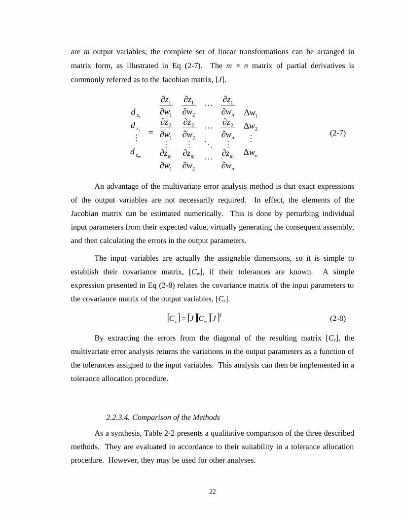
are m output variables; the complete set of linear transformations can be arranged in

matrix form, as illustrated in Eq (2-7). The m × n matrix of partial derivatives is

commonly referred as to the Jacobian matrix, [J].

∆

∆∆

∂∂

∂∂

∂∂

∂∂

∂∂

∂∂

∂∂

∂∂

∂∂

=

n

n

mmm

n

n

z

z

z

w

w

w

w

z

w

z

w

z

w

z

w

z

w

zw

z

w

z

w

z

m

M

L

MOMM

L

L

M2

1

21

2

2

2

1

2

1

2

1

1

1

2

1

δ

δδ

(2-7)

An advantage of the multivariate error analysis method is that exact expressions

of the output variables are not necessarily required. In effect, the elements of the

Jacobian matrix can be estimated numerically. This is done by perturbing individual

input parameters from their expected value, virtually generating the consequent assembly,

and then calculating the errors in the output parameters.

The input variables are actually the assignable dimensions, so it is simple to

establish their covariance matrix, [Cw], if their tolerances are known. A simple

expression presented in Eq (2-8) relates the covariance matrix of the input parameters to

the covariance matrix of the output variables, [Cz].

[ ] [ ][ ][ ]Twz JCJC = (2-8)

By extracting the errors from the diagonal of the resulting matrix [Cz], the

multivariate error analysis returns the variations in the output parameters as a function of

the tolerances assigned to the input variables. This analysis can then be implemented in a

tolerance allocation procedure.

2.2.3.4. Comparison of the Methods

As a synthesis, Table 2-2 presents a qualitative comparison of the three described

methods. They are evaluated in accordance to their suitability in a tolerance allocation

procedure. However, they may be used for other analyses.

23

Table 2-2: Comparison of Methods for Analyzing System Variability

Monte Carlo

Simulation

Analytical Model

Multivariate Error

Analysis Simplicity of establishing the algorithm, once the mathematical model is known

Good Regular Regular

Transparency of the algorithm, when bringing modifications or corrections

Good Bad Regular

Repeatability of the results Good Very good* Very good

Computing speed Very bad Very good Regular

Ability to allocate tolerances On simple assemblies

Regular Very good Good

Ability to allocate tolerances on complex assemblies

Bad Regular Good * Subject to independence of output variables

In conclusion, Monte Carlo simulation is relatively easy to establish, but is not

really suitable for tolerance allocation; it can be used to verify the results of the other

methods by performing a tolerance analysis, though. The analytical model is very

efficient if the assembly is not too complex; it presents great advantages, but also suffers

notable drawbacks. Finally, multivariate error analysis provides a good compromise of

computing characteristics that makes it very interesting for allocating tolerances in

general.

2.3. Least Cost Tolerance Allocation

2.3.1. Introduction

First of all, it is important to note the difference between tolerance analysis and

tolerance allocation. Tolerance analysis calculates the performance of a system for a

given set of fixed tolerances, while tolerance allocation selects the tolerances to assign so

that the system can satisfy its functional requirements. The objective of the presented

work is to minimize the manufacturing cost of an exactly constrained system. This cost

is affected by the values of the tolerances assigned to the different dimensions of the

system. The current problem is then a least cost tolerance allocation.

24

On one hand, making tight tolerances increases the manufacturing cost of the

system. On the other hand, if the tolerances are too large, the accuracy of the entire

system may be so affected that it may not be able to fulfill its functional requirements

anymore. A compromise between cost minimization and functionality of the product

then has to be established. This can be done by finding the best set of tolerances that

allows the system to keep respecting its functionality for the least cost possible. Hence

the problem is expressed as a minimization subject to constraints. An optimization

algorithm has to be established, in which the tolerances can be modified so that the

manufacturing cost can be lowered while the performance of the system stays at an

acceptable level.

Least cost tolerance allocation may be identified as a fundamental problem in

industry: finding a balanced compromise between precision and mass production. In

effect, precision is represented by the functional requirements of the system, while

manufacturing cost is a major concern in mass production. The proposed way to solve

this problem is an optimization procedure. However, optimization techniques may be

used in many other disciplines or even other engineering analyses [27].

2.3.2. Tolerance Allocation by Optimization

The real difficulty when dealing with an optimization problem is its formulation

for computational purposes. Once the different elements of the problem are identified

and expressed in a mathematical form, it is relatively easy to write the corresponding

algorithm, and some software packages can solve it with a specific optimization toolbox.

This section presents the elements to identify in order to solve the current problem, which

is a minimization subject to constraints.

The first entities to identify are the design variables. They are the quantifiable

parameters that can be changed by the algorithm while looking for the optimized

solution. These elements should be linearly independent in order to avoid conflicting

solutions. In effect, if several specifications can define one single design variable, they

may be contradictory when the optimization program is run, so it would be impossible to

return a properly optimized value for the design variable concerned. In the current

25

problem, the design variables are the tolerances in the exactly constrained assembly.

Assuming they are expressed as deviations from the nominal dimensions, their values

should be positive. Moreover, for satisfying the independence requirement, one single

value should represent a group of tolerances made by the same elementary manufacturing

sequence. In effect, it is impossible to make different levels of tolerance during the same

manufacturing process; so all the tolerances made by one sequence are strongly

correlated.

The second feature to identify is the objective of the optimization. It is a function,

depending on the design variables, that has to be optimized. For least cost tolerance

allocation, the objective function is the manufacturing cost that has to be minimized. It

should be expressed in terms of the values of the assignable tolerances; it is then

necessary to establish mathematically some cost / tolerance functions. This topic will be

discussed in the next section.

Finally, the system may be subject to constraints. They can be defined either as

equalities or as inequalities, influenced by the design variables. Constraint functions are

then bounded by limits, which are the functional requirements of the system. There may

be multiple constraints, one for each requirement of the system. For the tolerance

allocation problem, the constraints are expressed as inequalities. They are the deviations

resulting from the combinations of the assignable tolerances, which are the design

variables. These combinations are made with one of the different techniques presented in

Section 2.2.3 that establish a mathematical model of the system. These final deviations

characterize the performance of the system, so they shouldn’t be greater than a defined

limit, otherwise the system won’t be able to fulfill its functional requirements.

2.3.3. Cost / Tolerance Relations

The objective function of the tolerance allocation procedure requires an

expression of the manufacturing cost of the assembly as a function of the tolerances. It is

then necessary to establish cost / tolerance relations. There exists a notable amount of

publications dealing with this subject for metal removal processes. Chase [10] provides

26

an efficient synthesis of these studies, with empirical functions describing the

relationships between tolerance and cost.

For material removal processes, the tolerances can be tightened or loosened by

modifying the manufacturing parameters, such as feed, cutting speed, or depth of cut.

Quality of tooling, of fixtures, and of cutting tools also affects the tolerances and the

manufacturing cost. In addition, the workpiece may also be changed by selecting a more

machinable alloy. All these parameters create a relation between tolerances and

manufacturing cost. It is nearly impossible to predict analytically these relations; hence

empirical models have to be established from experimental data.

The manufacturing cost of a dimension depends upon several parameters:

• The selected manufacturing process. The existing material removal processes don’t

produce the same tolerancing deviation for the same operating cost. Some of them are

suitable for roughing operations, while other ones are adapted for finishing sequences.

Moreover, some processes are only efficient for a given range of dimensions. A

manufacturing cost should then be defined for every material removal process.

• The dimension’s nominal value, also known as the range. It is more expensive to

hold a given tolerance for a big dimension than for a smaller one. Cost / tolerance

relations then depend upon the range of the manufactured dimensions.

• The assigned tolerance. Tightening tolerances increases cost. This is the design

variable that can be modified to adjust the cost, once the nominal dimension is defined

and the manufacturing process is selected.

Different sets of experiments were run while varying these three parameters, and

the resulting cost was estimated. This cost was expressed in a relative way to eliminate

the effects of inflation. The resulting experimental data were treated by a curve fit

procedure to establish empirical relations. According to Chase’s researches, the

reciprocal power equation presented in Eq (2-9) looks to be an appropriate function to

represent the variable part of cost / tolerance relations.

27

β

α

Tolerance

RangeACost ×= (2-9)

where A, α and β are positive constants depending on the selected manufacturing process.

Once the design of the assembly is fixed and the manufacturing process is

selected, it is possible to transform this equation into a direct relation between cost and

tolerance. One function will then be specific to one assignable dimension.

Relations for material removal processes have already been established.

However, cost / tolerance functions for other manufacturing processes have not yet been

analyzed in a broad scope. Further investigation should be conducted in this field for

establishing a complete analysis of the possible cost / tolerance relations.

2.4. Chapter Summary

Exact constraint theory, analysis of manufacturing variations, and concepts of

optimization are used to establish a method for allocating tolerances to kinematic

systems. The procedure can be divided into four major steps:

• Describe the geometry and dimensional variations in a mathematical form. This is

done by establishing a parametric model of the assembly in order to characterize the

performance of the system as a function of its manufacturing variations, as described in

Section 2.2.2. This method is especially suitable for exactly constrained systems, as

explained in Section 2.1.

• Combine dimensional variations within the assembly to estimate resulting variation

in the system. Monte Carlo simulation, analytical modeling, and multivariate error

analysis are some of the mathematical tools that can be used for performing this

combination; they are presented in Section 2.2.3.

• Relate resulting variations to the performance requirements of the system. This is

specific to the functionality of every system, so there is no general method that can be

presented. However, the functional requirements of a mechanical assembly are related to

the assembly variation, previously calculated.

28

• Relate dimensional tolerances to manufacturing cost. Since the problem is a least

cost tolerance allocation, the objective is to minimize the cost of the system by

adequately assigning its tolerances. Cost / tolerance relations are then needed; they are

presented in Section 2.3.3.

These four steps are included in an optimization algorithm illustrated in Fig 2-1.

This program varies the tolerances of the assembly in order to find the minimum

manufacturing cost while respecting the functional requirements of the system. There

exist different methods for combining the manufacturing variations. One should be

selected advisedly, in accordance with the complexity of the system.

An optimization procedure is performed on one fixed design, for which the

nominal dimensions and the manufacturing processes have been previously selected.

Different design or manufacturing concepts can be compared by simply modifying the

input data of the optimization, then comparing the resulting costs provided by the

different tolerance allocations.

29

Start

Establish Parametric Modelof the Kinematic System

Input Nominal Dimensions forComponents of the System

Set of Tolerances as aStarting Guess

Calculate Assembly Variation

Input Limits onFunctional Requirements

Calculate Manufacturing Cost

Can the CostBe Reduced?

Yes

Select a New Setof Tolerances

Display Optimized Set ofTolerances and Minimized Cost

End

No

Calculate Performance

Fig 2-9: Flowchart of Least Cost Tolerance Allocation for Kinematic System

30

Chapter 3: Application to Optical Fiber Connectors

3.1. Introduction

3.1.1. Presentation

3.1.1.1. Fiber Optics

Until the 1980s, copper cables carried most electronic communication. Then

optical fibers were introduced, where light signals replace the electrical ones. An optical

fiber is a transparent rod, usually made of glass or clear plastic, through which light may

propagate. Its structure consists of a core, where light travels, coated with a cladding, as

illustrated in Fig 3-1. A jacket can eventually protect the fiber.

Protective JacketCladding

Core

Fig 3-1: Structure of an Optical Fiber

The core and the cladding have different optical characteristics. The core

refractive index is slightly greater than the cladding one; hence light stays inside the core

and reflects against the core/cladding interface. For typical communication fibers, the

cladding diameter is ~ 125 µm. The core diameter can vary a lot, depending on the

nature of the fiber. For multimode fibers, in which light propagates in many modes, the

core diameter is commonly ~ 50 µm. For single-mode fibers, the core diameter can vary

from 5 to 12 µm.

Fiber optic communication presents numerous advantages compared to other

communication methods [28]:

31

• Transmission loss is relatively low; thus long-distance transmission is possible

without using a costly amplification system,

• Fiber is lighter than copper cable,

• An optical fiber can carry more information than an equivalent copper cable can,

• There is a complete electrical isolation between the sender and the receiver,

• There is no interference in the transmission of light from electrical disturbances or

electrical noise,

• Optical fiber is more reliable, since it is not subject to corrosion and can better

withstand environmental conditions,

• Communication is more secure since it is impossible to intercept the light signal from

outside,

• The manufacturing cost of a fiber optic communication system is lower than the cost

of an equivalent cable communication system.

3.1.1.2. Transmission Losses

As shown in Eq (3-1), transmission coefficient (T) is defined as the ratio of the

output signal power (Pout) over the input signal power (Pin), where both powers are

expressed in the same units while the transmission coefficient is a non-dimensional

number.

in

out

P

PT = (3-1)

It is often convenient to express signal loss in decibels, with the relation given in

Eq (3-2). Since the transmission coefficient T is a number between 0 and 1, loss in

decibels is always a negative number. However, it is common to talk only of its absolute

value because loss implies the negative sign.

×=

in

outdB P

PLoss 10log10 (3-2)

32

Transmission loss is relatively low in fiber optic communication. In effect, a

common copper cable reduces the signal power to ~ 1% of its input value after one

kilometer, which represents a 20 dB loss, while a non-interrupted single-mode fiber can

typically carry up to 96% of the signal on the same distance, which corresponds to a 0.16

dB loss. Signal loss increases with fiber length, so for comparison purposes, most of the

calculations refer to a standard length of one kilometer.

There exist three main sources of light loss in a fiber [28]:

• Material loss. Absorption occurs when light interacts with the molecular structure of

the material. Impurities inside the fiber may increase this signal loss.

• Light scattering. Molecules, impurities and structural imperfections of the material

scatter light, which stops propagating and is lost.

• Bend loss. In practical applications, an optical fiber never follows a straight line but

instead is curved. If the radius of curvature is too small, light can’t reflect correctly on

the core/cladding interface and is dissipated.

These losses are wavelength dependent. For most applications, the greater the

wavelength, the lower the loss, but some applications need a specific wavelength. These

losses occur inside the fiber. On the other hand, connection losses generally have more

important consequences. For instance, a lateral misalignment of 1 micron between two

connected single-mode fibers generates a 0.21 dB signal loss.

As illustrated in Fig 3-2, there exist three types of connection losses [28] that are

directly related to the positional manufacturing errors within the connectors:

• Lateral misalignment is due to the offset of the centerlines of the mating fibers,

• End-separation misalignment comes from the gap between the ends of the connected

fibers,

• And finally, angular misalignment occurs when there exists an angle between the two

axes of the fibers.

33

Offset

Lateral MisalignmentEnd-SeparationMisalignment

Gap

Angular Misalignment

Angle

Fig 3-2: Misalignments Generating Connection Losses Between Mating Fibers

Every one of these misalignments generates a loss that can be calculated thanks to

analytical formulae found in literature [29]. The lateral misalignment is of most concern

for connection loss since angular misalignment is negligible and end-separation is usually

resolved by mechanical contact between the fibers or index-matching compounds.

Optical fiber connectors should then limit in priority this kind of misalignment in order to

improve efficiently their performance.

Polishing the end surfaces of the fibers is also important for limiting connection

loss. In the current study, it is assumed that the quality of the polishing operation is ood

enough to ignore the resulting connection loss compared the one generated by the lateral

misalignment.

3.1.1.3. Optical Fiber Connectors

Most of the mass-produced connections for optical fibers are made by mechanical

connectors, which are separable and relatively economical. However, these devices have

to be manufactured accurately to align correctly the fiber cores.

A common type of array connector is an assembly of two mechanically

transferable (MT) ferrules aligned by pins. An MT ferrule holds the fibers in position by

locating features such as cylindrical channels or vee-grooves. An aligning pin is housed

in a cylindrical hole of a theoretically equal diameter, but manufacturing variations for

the pin and the MT ferrule make this purely theoretical equality impossible. If the

diameter of the hole is greater than the diameter of the pin, there is a clearance between

them and the assembly is under-constrained. If the hole has a smaller diameter than the

pin, the system is over-constrained and there is an elastic or plastic deformation of the

34

components that affects their accuracy. In both cases, precision of the alignment is

notably affected.

A solution to avoid these effects is to design the ferrules so that the components

are exactly constrained when assembled together. The concept of the connector is

illustrated in Fig 3-3. A kinematic analysis of this assembly is presented in Section 3.2.1.

Fig 3-3: Optical Fiber Connector with Kinematically Designed Ferrules

These connectors are used in a passive alignment configuration: the fibers are

directly put into the ferrules to be aligned; no improvement system is applied to correct

their positioning; therefore the lateral misalignment between two mating fiber cores

depends directly on the dimensional and geometric variations of the components.

3.1.2. Background and Prior Work

Transmission loss is a major issue when connecting optical fibers. When fiber

optics communication was introduced, most of the current manufacturing processes

couldn’t attain the precision required for making mechanical connectors that could

Flexible Holder

Flexible Holder

Male Ferrule

Female Ferrule

Fiber Ribbon

Fiber Ribbon

35

provide a reasonable coupling efficiency by simply aligning two fibers. Some

sophisticated techniques were then developed. For instance, lenses could expand the

light beam at the end of the cores [30], micro actuators could improve the fiber alignment

[31], or the core diameters could be artificially increased by thermal expansion [32].

However, these techniques substantially increase the manufacturing cost of the

connectors.

Recent developments in manufacturing have made possible the production of

mechanical connectors capable of positioning the fibers with suitable accuracy [33]. The

resulting passive alignment is now so efficient that it is possible to avoid the correcting

systems previously mentioned. This solution is a way to reduce the number of parts

within the connector, and consequently its manufacturing cost.

Production of optical fiber connectors can involve various manufacturing

processes, like injection molding [34], LIGA technique [35] or etching [36], and different

materials [37,38]. Manufacturing variations are a critical issue in connector design [39].

In effect, manufacturing errors generate misalignments that increase transmission loss

[29]. Prior research performed tolerance analyses on MT ferrules using Monte Carlo

simulation [40] or analytical techniques [41].

This chapter describes a tolerance allocation technique for kinematically designed

connectors which is more efficient than the existing methods used for MT ferrules. The

developed procedure is based upon an exact mathematical model of the connector, which

improves the reliability of the method. The technique has been experimented with

Matlab∗ scripts. Monte Carlo simulations, also computed in Matlab, have been built to

verify the results of the tolerance allocation.

3.1.3. Tolerance Allocation

A rigorous tolerance allocation performed on the exactly constrained connector is

based upon a four-step algorithm, as described below.

∗ Matlab for Windows is software from The MathWorks, Inc., 24 Prime Park Way, Natick, MA.

36

• Describe the geometry and dimensional variations in a mathematical form. A

parametric model for every component of the connector is established as a function of the

nominal dimensions and the corresponding dimensional variations. Since the design of

the current connector follows the exact constraint theory, a kinematic analysis of the

connections among the different parts supplies a unique solution for the respective

location of the components. This solution, accurate and reliable, can be expressed

mathematically in a parametric model of the whole assembly.

• Combine dimensional variations in the connector to estimate misalignment of mating

fibers. The dimensional variations of the connector are directly related to its assigned

tolerances. The dimensional errors within the connector generate a misalignment

between the mating fibers. Applying the law of error propagation on the mathematical

model of the assembly provides an analytical relation between dimensional variation and

fiber misalignment. The unique solution of the mathematical model due to the exact

constraint theory makes this approach possible.

• Relate assembly variations to the performance requirements of the connector. The

performance of a connector is defined by its capacity to transmit light with as little loss as

possible. Connection losses dependent on a mechanical connector are directly related to

the misalignments generated by the manufacturing errors of the components. When

considering realistic manufacturing variations, lateral misalignment is the most critical

parameter. The lateral misalignment between two mating fibers therefore characterizes

the performance of a connector. Since the present connector aligns arrays of multiple

fibers, its performance will be defined with regard to the maximum misalignment

observed in the whole array.

• Relate dimensional tolerances to manufacturing cost. This connector will be mass-

produced; hence its manufacturing cost has to be minimized. The magnitude of the

acceptable lateral misalignment determines the manufacturing processes that should be

used for making the connector. Once the production sequence is selected, it is possible to

express the manufacturing cost as a function of the assigned tolerances using cost-

tolerance functions.

37

The algorithm presented in Fig 3-4 includes these four steps. The law of error

propagation, applied to the mathematical model of the connector, returns an analytical

relation between lateral misalignment and manufacturing tolerances. In parallel, cost-

tolerance functions are used to calculate the resulting manufacturing cost. The process is

implemented in an optimization loop.

Start

Input Nominal Dimensions forComponents of the Connector

Input Fixed Tolerancesfor Pins and Fibers

Set of Tolerances for Ferrulesas a Starting Guess

Establish Parametric Modelof the Connector

Establish Partial Derivatives of Misalignmentswith Respect to Assignable Dimensions

Input Constraints onAcceptable Misalignments

Calculate Misalignments byLaw of Error Propagation

Calculate Manufacturing Cost

Can the CostBe Reduced?

Display Optimized Set of Tolerancesand Minimized Cost

End

Yes

No

Select a New Setof Tolerances

Fig 3-4: Flowchart of the Tolerance Allocation for Optical Fiber Connector

38

3.2. Mathematical Model

3.2.1. Exact Constraints Within the Connector

The exactly constrained connector follows the rules of kinematic design theory.

The main requirement of this feature is two align mechanically two arrays of fibers.

Every fiber is located in a vee-groove: there is a cylindrical contact between a fiber and

its corresponding ferrule. The two ferrules are aligned by two pins. The male ferrule is

connected to the first pin by a vee-groove, and to the second pin by two planes; in both

cases, it is a cylindrical contact. The female ferrule has a different design to avoid

redundant constraints. In effect, a vee-groove still makes a cylindrical contact between

the first pin and the ferrule, but a single plane is touching the second pin for making a

linear contact. Finally, the different elements are maintained in position by flexible clips.

The corresponding kinematic mapping of the connector is illustrated in Fig 3-5, while its

kinematic diagram is represented in Fig 3-6 with four pairs of fibers.

MaleFiber

Cylindrical MaleFerrule

FirstPin

SecondPin

FemaleFerrule

Cylindrical

Cylindrical

FemaleFiber

Cylindrical

Cylindrical

Linear

Fig 3-5: Kinematic Analysis of the Exactly Constrained Connector

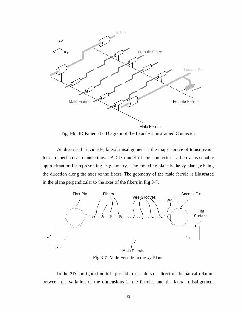
39

x

y

z

Male Ferrule

Female FerruleMale Fibers

Female Fibers

First Pin

Second Pin

Fig 3-6: 3D Kinematic Diagram of the Exactly Constrained Connector

As discussed previously, lateral misalignment is the major source of transmission

loss in mechanical connections. A 2D model of the connector is then a reasonable

approximation for representing its geometry. The modeling plane is the xy-plane, z being

the direction along the axes of the fibers. The geometry of the male ferrule is illustrated

in the plane perpendicular to the axes of the fibers in Fig 3-7.

FibersFirst PinVee-Grooves

Second Pin

Male Ferrulex

y

FlatSurface

Wall

Fig 3-7: Male Ferrule in the xy-Plane

In the 2D configuration, it is possible to establish a direct mathematical relation

between the variation of the dimensions in the ferrules and the lateral misalignment

40

between two mating fibers. Since the components are exactly constrained, there is a

unique solution for the location of a connection point between two features.

3.2.2. Parametric Model of the Components in the Connector

3.2.2.1. Presentation

The tolerance allocation process is based upon a mathematical model of the

assembly that includes the dimensions of the components and their respective variations

due to the manufacturing errors. These variations appear at different levels of the

assembly. First of all, the fibers have variations that can be represented in 2D as shown

in Fig 3-8. If the fiber is perfect, its core and its cladding are concentric and perfectly

circular with known diameters. But in a real case, the manufacturing errors affect the

dimensions and the shape of a fiber.

PerfectDiameter

of Cladding

Core isConcentric to

Cladding

PerfectDiameterof Core

PerfectlyCircularCladding

CircularityVariation inCladding

Variation inDiameterof Core

Variation inDiameter

of Cladding

ConcentricityVariation

Perfect Fiber Real Fiber

Fig 3-8: 2D Model of a Perfect Fiber and a Real Fiber

The defects previously presented are only for individual fibers. The variations of

the ferrules and the alignment pins will also affect the accuracy of the alignment of a

whole array of fibers. In theory, this array is a perfectly straight line with a constant pitch

between two successive fibers, as illustrated in Fig 3-9. Manufacturing errors in the

different components of the connector induce variations in the positioning of the fibers

within the array. Fig 3-10 presents some relevant variations that can happen in an array

because of the manufacturing errors.

41

Colinearity of AllFibers in Array

No Skewnessof Fiber Line

Perfect PitchBetween Two

Successive Fibers

PerfectFiber

Fig 3-9: 2D Model of a Perfect Array of Fibers

Variation inColinearity of Fibers

Skewness ofFiber Line

ImperfectFiber

Variation inPitch Between

Successive Fibers

Fig 3-10: 2D Model of an Array of Fibers with Manufacturing Variations

Finally, the function of a connector is to mate two arrays of fibers. Both arrays

have their dimensional and geometric variations, as explained before. When mating the

arrays, the errors in the fibers, the ferrules, and the alignment pins are combined and

produce a lateral misalignment in every pair of mating cores, as shown in Fig 3-11. The

parametric model to be established should calculate this lateral misalignment as a

function of the manufacturing errors within the different components of the connector, by

mathematically expressing this combination of variations.

42

Fig 3-11: 2D Model of Mating Arrays of Fibers with Manufacturing Variations

The manufactured dimensions are interpreted as variables in the mathematical

model. This section presents how the different components with their respective errors

are parametrically represented. Since a statistical treatment will be performed on the

mathematical model, the dimensions subject to manufacturing errors are expressed as

randomly distributed variables, with an expected value equal to their nominal dimension

and a standard deviation related to their assigned tolerance. Identification of their

distribution is important too.

3.2.2.2. Pins and Fiber Claddings

Two pins align the ferrules, and the fibers are located by vee-grooves. These

cylindrical features are represented by circles in the 2D model. The diameter is the only

dimension that is important for positioning the fibers, since the length of the pins is not

taken into consideration in the 2D model. The diameter can vary by its scalar dimension,

represented by its magnitude, or by its geometry, defined by its non-circularity, as

illustrated in Fig 3-12.

43

(a) Biggerdiameter

(d) 5-lobenon-circularity

Legend: Perfect pinReal pin

(b) Smallerdiameter

(c) 2-lobenon-circularity

Fig 3-12: Different Possible Errors in a Cylindrical Feature

Knowing the radius of a cylinder is particularly important at the two contact

points with the corresponding vee-groove. The parametric model of a random cylinder

first defines its average radius as a normally distributed variable: this deals with the

strictly dimensional variation of the feature. Then at both contact points, the average

radius is multiplied by a random coefficient that stands for the non-circularity of the

feature: this is its geometric variation. This coefficient is a normally distributed variable,

with an expected value of 1.

3.2.2.3. Cores of Fibers

A fiber is aligned by its cladding in contact with a vee-groove of the ferrule. But

light is transmitted through the core of the fiber. Thus the errors of the core position

relative to the cladding should be taken into consideration.

In a perfect fiber, the core is exactly concentric to the cladding. In a real one,

there may be an eccentricity that can be quantified by the fiber manufacturer. The

mathematical model represents this eccentricity with two parameters: its magnitude,

which is a normally distributed variable whose expected value equals 0, and its location

angle, which is a uniformly distributed variable varying from 0 to 180 degrees. Note that

it is not necessary to distribute this angle on a 360-degree range, since the normally

distributed magnitude can have a negative value.

Geometry of the core itself can also vary. Its diameter is expressed as a normally

distributed variable. Its non-circularity has a negligible effect on the transmission loss,

44

compared to the other sources of errors. Then a core is assumed to be perfectly circular;

this approximation simplifies the mathematical model without affecting its accuracy.

3.2.2.4. Ferrules

The fibers tolerances are determined by industry standards. On the oter hand, it is

possible to control the tolerances on the ferrules and the pins to reduce production cost

while respecting the functional requirements of the connectors. The geometry of a ferrule

is parametrically represented in 2D by a set of lengths and angles, as illustrated in Fig

3-13. All these dimensions are normally distributed variables in the mathematical model.

PitchFlat

Pitch PinAngle Flat

x

y

See Detail A

Depth Pin DepthFiber

DepthFlat

Detail A

Half-AnglePin

Half-AngleFiber

Fig 3-13: 2D Parametric Representation of a Ferrule

Distances in the x-direction between vee-grooves are referred to as pitches. A

complete parametric model of the ferrule requires three pitches: pitch between the pin

vee-groove and the closest fiber vee-groove (identified as “Pitch Pin” in Fig 3-13), pitch

between two successive fiber vee-grooves (“Pitch Fiber”), and finally pitch between the

wall positioning the second pin and the closest fiber vee-groove (“Pitch Flat”).

Since these dimensions only locate the grooves in the x-direction, another set of

lengths is needed for positioning them in the y-direction. These dimensions are called

“depth,” and they represent the distance between the vertex of a vee-groove and a datum

45

plane, shown as the bottom of a perfect ferrule in Fig 3-13. The vertex of a groove is

actually a virtual point, since it is hidden by the radius of curvature present at the bottom

of the groove. Once again, there are three different dimensions for the whole ferrule.

The first depth is used by the pin vee-groove (“Depth Pin”). The second one locates the

fiber grooves (“Fiber Depth”). The third one is finally the distance between the datum

plane and the flat surface positioning the second fiber (“Depth Flat”). This flat surface is

modeled in the parametric representation as perfectly parallel to the datum plane; any

form variation of the surface, such as flatness error or parallelism error, is included in the

variation of the depth. This statement is acceptable because the pin and the ferrule are

exactly constrained, so their contact is reduced to one single point in the 2D

representation.

The parametric model of the ferrule is completed by the angles of the vee-

grooves. These features are used to locate the first pin and the fibers. Two angles affect

the accuracy of a vee-groove: its aperture angle, and its inclination angle, which is the

angle between its bisector and the y-axis. Metrology applied to a ferrule cannot directly

measure the value of the inclination angle, so it was decided to represent the vee-groove

as a combination of two half-angles. The aperture angle is defined as the sum of the two

half-angles while the inclination angle is calculated as half their difference. Hence the

parametric model uses half-angles for the pin vee-grooves (“Half-Angle Pin”) and for the

fiber grooves (“Half-Angle Fiber”).

The second pin is positioned in the male ferrule by a flat surface and a wall. The

mathematical model combines these two surfaces to define them as a single vee-groove.

However, since the flat surface is defined as perfectly parallel to the x-direction, there is

no need to model an inclination angle for this groove. Its aperture angle (“Angle Flat”) is

sufficient to represent mathematically its geometry and the related variations.

3.2.2.5. List of the Variables

The previous sections present how the variables included in the parametric model

of the connector are defined. Table 3-1 summarizes these randomly distributed variables

with their respective distributions.

46

Table 3-1: Variables Used in the 2D Parametric Model of the Connector

Dimension Distribution

Average diameter Normal Pi

n

Non-circularity Normal centered on 1

Average diameter of cladding Normal

Non-circularity of cladding Normal centered on 1

Diameter of core Normal

Magnitude of core eccentricity Normal centered on 0

Fibe

r

Angle of core eccentricity Uniform on a 180-degree range

Pitch between pin and closest fiber Normal

Pitch between two successive fibers Normal

Pitch between wall and closest fiber Normal

Depth of pin vee-groove Normal

Depth of fiber vee-groove Normal

Depth of flat surface Normal

Half-angle of pin vee-groove Normal

Half-angle of fiber vee-groove Normal

Ferr

ule

Angle between wall and flat surface Normal

3.2.3. Mathematic Description of the Geometric Model

3.2.3.1. Assembly of a Random Cylinder Inside a Random Vee-Groove

Knowing the real location of a cylindrical feature in a vee-groove is of primary

interest for modeling the geometry of the connector, since the pins and the fibers are

located by vee-grooves. The advantage of such an assembly is that the resting position of

the cylindrical feature is defined by only two lines, which is equivalent to an exact

constraint for a 2D model. Hence there can only be one resting position for one given

cylinder and one vee-groove if the effects of friction and stiffness of the features are

neglected. The geometry of a non-round cylinder in a real vee-groove is illustrated in Fig

3-14.

47

φL

φR

V

RL

RR

MR

ML

C

y

x

Fig 3-14: Location of a Random Cylinder in a Random Vee-Groove

The geometry of the groove is defined by two angles: φL is the angle between the

left edge of the vee-groove and the vertical, and φR is the one for the right side. The non-

round cylinder (pin or fiber) is put inside the vee-groove. C is the center of the non-

round cylinder. V is the vertex of the vee-groove. ML and MR are respectively the

contact points of the cylinder with the left edge of the vee-groove and with the right edge.

Consequently, CML and CMR are respectively the radii of the cylinder on the left side and

on the right side. The goal is to find the coordinates of vector CV . The known

dimensions are the radii CML and CMR, and the angles Lφ and Rφ .

At the contact points ML and MR, the non-round cylinder locally acts like a

perfect cylinder, so the edges are perpendicular to the respective radii at these contact

points, which gives Eqs (3-3)-(3-4):

2

π=∠ CVM L (3-3)

2

π=∠ VCM R (3-4)

From the geometry of triangle (CMLMR), we can get the relation shown in Eq

(3-5):

48

( )LRRLRLRL CMMCMCMCMCMMM ∠⋅⋅⋅−+= cos222 (3-5)

On the other hand, the geometry of quadrilatere (CMLVMR) provides Eq (3-6):

CVMVCMVMMCMM LRLRRL ∠−∠−∠−=∠ π2 (3-6)

Inserting Eqs (3-3)-(3-4) in Eq (3-6) gives Eq (3-7):

LRRL VMMCMM ∠−=∠ π (3-7)

Trigonometric relations applied to Eq (3-7) leads to Eq (3-8):

( ) ( )LRRL VMMCMM ∠−=∠ coscos (3-8)

Eq (3-9) is obtained by expressing Eq (3-8) in terms of the known dimensions:

( ) ( )RLRLCMM φφ +−=∠ coscos (3-9)

Eq (3-5) can now be modified by inserting Eq (3-9) to become Eq (3-10):

( )RLRLRLRL CMCMCMCMMM φφ +⋅⋅⋅++= cos222 (3-10)

This equation fully defines the length MLMR with respect to known dimensions.

The next step deals with the geometry of triangle (CMLMR), which provides Eq

(3-11):

( )RLL

RRLLLR MMCM

CMMMCMCMM

⋅⋅−+

=∠2

cos222

(3-11)

Inserting Eq (3-10) in Eq (3-11) gives Eq (3-12), and by simplification Eq (3-13):

( )

⋅⋅

+⋅⋅⋅+⋅=∠

RLL

RLRLLLR MMCM

CMCMCMCMM

2

cos22arccos

2 φφ (3-12)

( )

+⋅+=∠⇒

RL

RLRLLR MM

CMCMCMM

φφcosarccos (3-13)

This last equation fully defines the value of angle RLMCM∠ with respect to

known dimensions.

49

Then the geometry of rectangle triangles (VMLC) and (VMRC) are taken into

consideration to establish Eq (3-14)-(3-15):

222 VCCMVM LL =+ (3-14)

222 VCCMVM RR =+ (3-15)

Combining these two equations results in Eq (3-16):

2222RLLR CMCMVMVM −+= (3-16)

At the same time, the geometry of triangle (VMLMR) is used to establish Eq

(3-17):

( )RLRLLRLLR MVMMMVMMMVMVM ∠⋅⋅⋅−+= cos2222 (3-17)

Equality of Eq (3-16) and Eq (3-17) results in Eq (3-18):

( ) 222 cos2 RLRLRLLRL RRMVMMMVMMM −=∠⋅⋅⋅− (3-18)

Eq (3-19) is obtained by inserting Eq (3-10) in Eq (3-18):

( )

( ) 22

22

cos2

cos2

RLRLRLL

RLRLLRL

CMCMMVMMMVM

MMVMCMCM

−=∠⋅⋅⋅−

+⋅⋅⋅++ φφ (3-19)

Trigonometric relations establish Eq (3-20):

( ) ( )CMMCMMMVM LRLRRL ∠=

−=∠ sin

2coscos

π (3-20)

This relation is inserted in Eq (3-19) to obtain Eq (3-21):

( )( )CMMMM

CMCMCMVM

LRRL

RLRLRL ∠⋅

+⋅⋅−=

sin

cos2 φφ (3-21)

Now the geometry of rectangle triangle (VCML) is observed to establish Eq

(3-22):

( )L

LL VM

CMCVM =∠tan (3-22)

50

Inserting Eq (3-21) in Eq (3-22) results in Eq (3-23):

( )( )

+⋅⋅+

∠⋅⋅=∠

RLRLR

LRRLLL CMCMCM

CMMMMCMCVM

φφcos

sinarctan 2

(3-23)

This equation fully defines angle LCVM∠ with respect to known dimensions.

The same triangle is used to obtain Eq (3-24):

( )L

L

CVM

CMCV

∠=

sin (3-24)

The coordinates of vector CV can finally be established with Eqs (3-25)-(3-26):

( )

( )

∠−⋅−=

∠−⋅=

LLCV

LLCV

CVMCVY

CVMCVX

φ

φ

cos

sin

(3-25)

(3-26)

By inserting Eq (3-24), these equations can be modified as shown in Eqs (3-27)-

(3-28).

( )( )

( )( )

∠∠−⋅

−=

∠∠−⋅

=

L

LLL

CV

L

LLL

CV

CVM

CVMCMY

CVM

CVMCMX

sin

cos

sin

sin

φ

φ

(3-27)

(3-28)

These last two equations fully define the coordinates of vector CV with respect

to known dimensions, in the local coordinate system of a ferrule.

3.2.3.2. Creating an Array of Fibers

The previous step presents a way to calculate the coordinates of a fiber or a pin in

its respective vee-groove. The following step is to define the coordinates of the fibers in

the same coordinate system. The general shape of a ferrule is illustrated in Fig 3-15:

51

h1 h2

V1 V2

C1

C2

x

RL2 RR2

εp2

ML1

MR2

ML2

MR1

y

Fig 3-15: Shape of a Random Ferrule in 2D

The temporary coordinate system (indexed A) is such that the bottom of the

ferrule is horizontal. The starting point is to define the coordinates of vector 21CC . This

vector can be decomposed like this: 22211121 CVVVVCCC ++= .

Coordinates of vector 11VC can be found with the method presented in Section

3.2.3.1. The x-coordinate of vector 21VV is a dimension defined by the designer. Its y-

coordinate can be defined by the dimension scheme presented in Eqs (3-29)-(3-30),

related to the bottom of the ferrule:

12 12hYhY V

AV

A −=− (3-29)

121221

hhYYY VA

VA

VV

A −=−=⇔ (3-30)

The second pin is assumed to lie on a horizontal surface, at the contact point MR2.

Triangle (V2MR2C2) is rectangle in MR2, so the coordinates of vector 22CV are given by

Eqs (3-31)-(3-32):

( )

=

∠=

22

222

22

22

22 tan

RCV

A

R

R

CV

A

MCY

CVM

MCX

(3-31)

(3-32)

Subsequently the coordinates of vector 21CC are given by relations presented in

Eqs (3-33)-(3-34):

52

( )222

22

tan211121 CVM

MCXXX

R

R

VV

A

VC

A

CC

A

∠++= (3-33)

22121121

RVC

A

CC

A MChhYY +−+= (3-34)

The coordinates of every fiber’s center are found with a similar dimension

scheme.

The next step is to set a new coordinate system, indexed B. Its center is still the

center of the reference pin, but the horizontal is now defined as the line going through the

centers of the two pins. Hence there is an angle εp2 between coordinate systems A and B.

The value of this angle can be defined with the coordinates of the vectors in coordinate

system A, as shown in Eq (3-35):

=

21

21arctan2

CC

A

CC

A

p X

Yε (3-35)

The manufacturing errors in a fiber vee-groove will create a similar offset angle

εf. The coordinates ( )fB

fB YX , of the center of a fiber in the coordinate system B are

then presented in Eqs (3-36)-(3-37):

( )222 cos pff

Af

Af

B YXX εε −×+= (3-36)

( )222 sin pff

Af

Af

B YXY εε −×+= (3-37)

Finally, the coordinates of the core of the fiber are calculated by taking into

consideration the eccentricity of the core deviating from the center of the fiber, as shown

in Eqs (3-38)-(3-39):

( )ecccorefB

coreB EccXX φcos⋅+= (3-38)

( )ecccorefB

coreB EccYY φsin⋅+= (3-39)

where Ecccore is the magnitude of the offset of the core and φecc is its orientation angle.

53

3.2.3.3. Mating Two Fibers

The coordinates of the centers of the fibers can be determined independently by

the method presented in the previous sections. Since the ferrules are aligned by the two

pins, the coordinate system B, whose origin is the center of the first pin and whose x-axis

is the line that goes through the center of both pins, is common to the two ferrules.

The core of a fiber in the male ferrule is modeled by its coordinates

( )coreMB

coreMB YX , . It has to be aligned with a core of a corresponding fiber in the female

ferrule; the coordinates of this second core are ( )coreFB

coreFB YX , . The lateral

misalignment d between the two mating cores is then:

( ) ( )22

coreFB

coreMB

coreFB

coreMB YYXXd −+−= (3-40)

When dealing with single-mode fibers, applying Marcuse’s model [29] on this

final result allows calculating the transmission loss in decibels due to the geometric

variations of the features assembled in the connector.

Transmission loss depends upon lateral misalignment but also upon the optical

properties of the fibers. Contrarily to multi-mode fibers, single-mode fibers work with a

specific wavelength λ (defined in meters). It is then possible to define a free space

propagation constant k (unit: m-1) for a single-mode connection, with Eq (3-41):

λπ2

=k (3-41)

Marcuse starts by defining a dimensionless Vi parameter for the ith fiber with Eq

(3-42):

( )22claddingcorei nnakV −⋅⋅= (3-42)

where ai is the core radius of the fiber (in m). This Vi parameter is used for defining the

width parameter wi (in m) of the ith fiber by the empirical formula presented in Eq (3-43):

++⋅= 6

23

879.2619.165.0

ii

iiVV

aw (3-43)

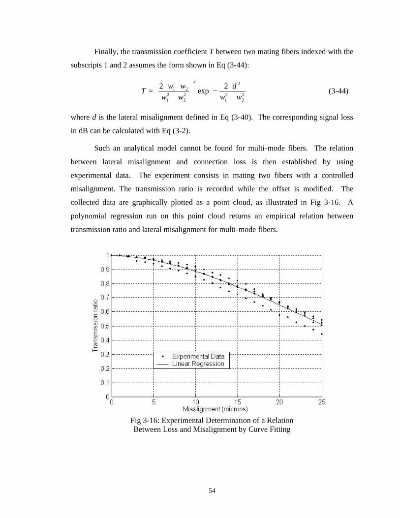
54

Finally, the transmission coefficient T between two mating fibers indexed with the

subscripts 1 and 2 assumes the form shown in Eq (3-44):

+⋅

−

+

⋅⋅=

22

21

22

22

21

21 2exp

2

ww

d

ww

wwT (3-44)

where d is the lateral misalignment defined in Eq (3-40). The corresponding signal loss

in dB can be calculated with Eq (3-2).

Such an analytical model cannot be found for multi-mode fibers. The relation

between lateral misalignment and connection loss is then established by using

experimental data. The experiment consists in mating two fibers with a controlled

misalignment. The transmission ratio is recorded while the offset is modified. The

collected data are graphically plotted as a point cloud, as illustrated in Fig 3-16. A

polynomial regression run on this point cloud returns an empirical relation between

transmission ratio and lateral misalignment for multi-mode fibers.

Fig 3-16: Experimental Determination of a Relation Between Loss and Misalignment by Curve Fitting

55

These equations constitute the parametric model of a connector by establishing a

mathematical relation between the transmission loss and the manufacturing dimensions

with their respective variations. The model is used in a tolerance allocation procedure to

ensure that the maximum acceptable transmission loss is respected while the

manufacturing cost is minimized.

3.3. Tolerance Allocation

3.3.1. Overview

This section presents a method for allocating tolerances to dimensions in exactly

constrained ferrules used to align optical fibers. The objective is to reduce the

manufacturing cost without exceeding a limit on the misalignment between two mating

fibers. The allocation procedure is performed on the 2D geometric model of the multi-

fiber connector developed in the previous section. An analytical representation of the

connection, based upon statistics, is used for providing a relation between variation in

manufactured dimensions and variation in the resulting misalignment of the fibers

contained in the array. Optimal tolerances are determined using a non-linear constrained

optimization algorithm that minimizes the manufacturing cost while satisfying constraints

on the variation of the misalignment of any pair of fibers in the array. The method

provides a useful tool when designing mass-produced connectors for multi-fiber cables,

for which manufacturing cost and accuracy are critical parameters.

The goal of this study is to select tolerances that are sufficient for aligning optical

fibers without excessive loss, but simultaneously minimize manufacturing costs that arise

from excessively tight tolerances. Tolerance allocation is generally formulated as an

optimization problem with an objective function and a set of constraints. In this case, the

objective is to minimize the manufacturing cost which is a function of the tolerances.

Tolerance relations for etched silicon parts are not available. However, for other

materials like zirconium, a secondary material removal process like grinding may

improve the tolerances. In this case, we employ relations developed by Chase [10] to

relate manufacturing costs to tolerances. Both cost and signal loss can be defined as

56

functions of the tolerances allocated by the designer. The optimization constraints are

formulated as maximum tolerable signal loss within an entire connector.

In formulating the optimization problem, the greatest challenge is determining a

relationship between the tolerances and the performance criteria. For complex

assemblies such as an optical fiber connector, Monte Carlo simulations are effective

means for relating final tolerance of an assembly to the tolerances of the components

[42]. However, it may be difficult to implement Monte Carlo simulations within the

optimization algorithm due to computational time. We instead use an alternative

approach in which a few Monte Carlo simulations provide a mathematical model relating

assembly tolerances to component tolerances. Knowing the geometry and the dimensions

of the connector, it is possible to define the signal loss of the fiber connection as a

function of the tolerances of the ferrules.

This section presents a process to efficiently allocate the tolerances for vee-

groove fiber alignment. The first step is to construct a mathematical model of the

dimensions and geometry of the connector, which was detailed in the previous section.

The second step is to define, through a statistical study, the misalignment of the fiber as a

function of the tolerances in the ferrules. The third step is to estimate a relation between

the tolerances and the manufacturing costs. Finally, tolerances are allocated with an

optimization algorithm that minimizes the manufacturing cost for a given maximum limit

on signal loss.

3.3.2. Variation Analysis by the Law of Error Propagation

Tolerance allocation requires a relation between dimensional variations and

connection loss. It is established by applying the law of error propagation [25] on the

mathematical model of the connectors. This method is computationally efficient when

used in a tolerance allocation algorithm.

The geometric model of the ferrules must be expressed in terms of statistics.

Every dimension ξi, presented in Table 3-1, is defined as a randomly distributed variable.

Its mean µi equals the value of the nominal dimension, while its standard deviation σi is a

57

third of the tolerance. For a complete representation of the connector, the same procedure

is applied for the dimensions of the fibers and the alignment pins.

The lateral misalignment dj for the jth pair of fibers is modeled as a vector in the

xy-plane. It is possible to define its coordinates, ( )jj dd yx , , as a function of the dimensions

of the ferrules, the fibers, and the pins, as shown in Eqs (3-45)-(3-46):

( )nixd jjfx ξξξξ ,...,,...,, 21= (3-45)

( )niyd jjfy ξξξξ ,...,,...,, 21= (3-46)

n being the total number of assigned dimensions within the connector.

According to the law of error propagation, if the dimensions are independent

(which is a reasonable assumption for most applications), then the standard deviations

jdxσ and jdyσ of the lateral misalignment in the x and y directions are given by Eqs

(3-47)-(3-48):

∑=

∂

∂≈

n

ii

i

x

xj

jd

f

1

2

2

2 σξ

σ (3-47)

∑=

∂

∂≈

n

ii

i

y

yj

jd

f

1

2

2

2 σξ

σ (3-48)

For perfect dimensions, the misalignment equals zero. Hence for random

dimensions, its variation is directly related to its standard deviation and does not depend

on its expected value. The law of error propagation then gives a direct analytical

expression of the variance in lateral misalignment as function of the variances in the

different dimensions of the connector. Since the current study analyzes the sensitivity of

the lateral misalignment to the geometry of the ferrules, the standard deviations related to

the dimensions of the fibers and the pins are considered as constants. Only the 9 standard

deviations defining the ferrules are identified as the variables to optimize.

Eqs (3-47)-(3-48) return the variances of the components in the x and y directions

for the lateral misalignment, but Marcuse’s model requires the magnitude of the

58

misalignment, dj. Its value could be expressed with a joint probability distribution for xd

and yd, but an unknown correlation coefficient between the two components compromises

the accuracy of the calculation. If the correlation coefficient were negligible, an exact

definition of the joint probability distribution could be established with the calculations

presented in Appendix A; however the value of the coefficient is too high to be neglected.

Therefore a Monte Carlo simulation of the connector is used to determine an empirical

relation between the connection loss and the standard deviations of jdx and

jdy by a two-

step process.

The first step consists in collecting data from the Monte Carlo simulation. Its

inputs are the nominal values and the tolerances of the different dimensions defining the

geometry of a connector. A large number of connectors are virtually generated using the

mathematical model previously presented. Their dimensions are normally distributed,

with a mean equal to their nominal value and a standard deviation equal to one third of

their tolerance. The algorithm calculates the misalignment of each randomly generated

sample; then it performs a statistical treatment on the collected results. Finally, it returns

the standard deviation of the components in x and y of the lateral misalignment, as well as

a cumulative distribution function (cdf) of the connection loss (in dB) for every pair of

fibers, as shown in Fig 3-17.

59

Fig 3-17: Outputs of Monte Carlo Simulation

Every cdf is curve fitted with a two-variable continuous function. Since the

tolerance analysis focuses on the highest part of the cdf (beyond 90%), the curve fitting is

performed exclusively on this part of the cdf in order to get more reliable approximations.

It has been found that for single-mode fibers, the cdf of a Weibull random variable is a

good approximation, while a Gamma incomplete function fits well the cdf of the multi-

mode fibers.

The simulation is run many times with different input tolerances. The resulting

cdf’s are reduced to two parameters defining the fitted curve. Hence the first step of the

process returns a set of values for the two fitting parameters as a function of the standard

deviations of jdx and

jdy .

The second step is a new curve fitting procedure. This time, one of the fitting

parameters is plotted as a function of the standard deviations of jdx and

jdy , and it is

60

curve fitted. The resulting relations are finally compared to new Monte Carlo

simulations, and it has appeared that they were extremely reliable. These functions are

used as empirical models of the connection loss.

Thereby a variation analysis based upon the law of error propagation, followed by

an empirical yet accurate model of the connector performance, provides a relation

between the connection loss and the tolerances of the ferrules.

3.3.3. Cost / Tolerance Functions

The cost of a manufactured part depends upon the selected manufacturing process

and dimensional tolerances. The cost of achieving a particular tolerance depends upon

both the dimension's nominal value and tolerance. The manufacturing cost generally

increases if the tolerance is tightened, and it is more expensive to make a given tolerance

on a large nominal dimension. Based on this, Chase [10] recommends expressing

tolerances as reciprocal power functions for material removal processes. Eq (3-49)

expresses the tolerance for the ith dimension, ti, as a function of cost, Ci, range, Ri, and

three constants ai, bi, and ci. The values of the three constants depend upon the range and

the manufacturing process. Although a constant term would be necessary for accuracy, it

is practically impossible to evaluate and doesn’t affect the tolerance allocation.

i

i

bi

ai

iiC

Rct ×= (3-49)

Similar functions are not available for etching processes commonly used with silicon.

Knowing the range and the manufacturing process of every dimension enables the

generation of the cost-tolerance functions required to estimate the manufacturing cost of a

connector as a function of the tolerances assigned to its different dimensions. The

portion of the total manufacturing cost that is attributable to ferrule tolerancing is the sum

of the costs for the successive manufacturing processes used for producing a ferrule.

61

3.3.4. Results of the Tolerance Allocation Algorithm

Optimal tolerances for the dimensions are determined using nonlinear constrained

optimization. The problem is formulated as a minimization subject to constraints. The

function to minimize is the manufacturing cost of the connector with respect to its

tolerances, as defined in the previous section. Constraints are formulated by specifying

that the standard deviation of the lateral misalignment, jdσ , for every pair of fibers

within the connector must be positive yet below a critical value. Additional bounds can

be specified to prevent the optimization from driving the assigned tolerances to

unreasonably high or low values.

Since this optimization only deals with allocating tolerances to the ferrules, it is

assumed that the tolerances for the fibers and the alignment pins are already known

empirically or predicted by another analysis. The variables of the optimization problem

are then the tolerances for the 9 dimensions defining the ferrules.

This method was used to allocate tolerances to an exemplary connector. The

objective was to minimize the manufacturing cost of an 8-fiber connector while the

connection loss of every pair of single-mode fibers should be less than 0.5 dB. The

calculated connection losses along the connectors are displayed in Fig 3-18, and the

resulting tolerances allocated by the optimization procedure are listed in Table 3-2.

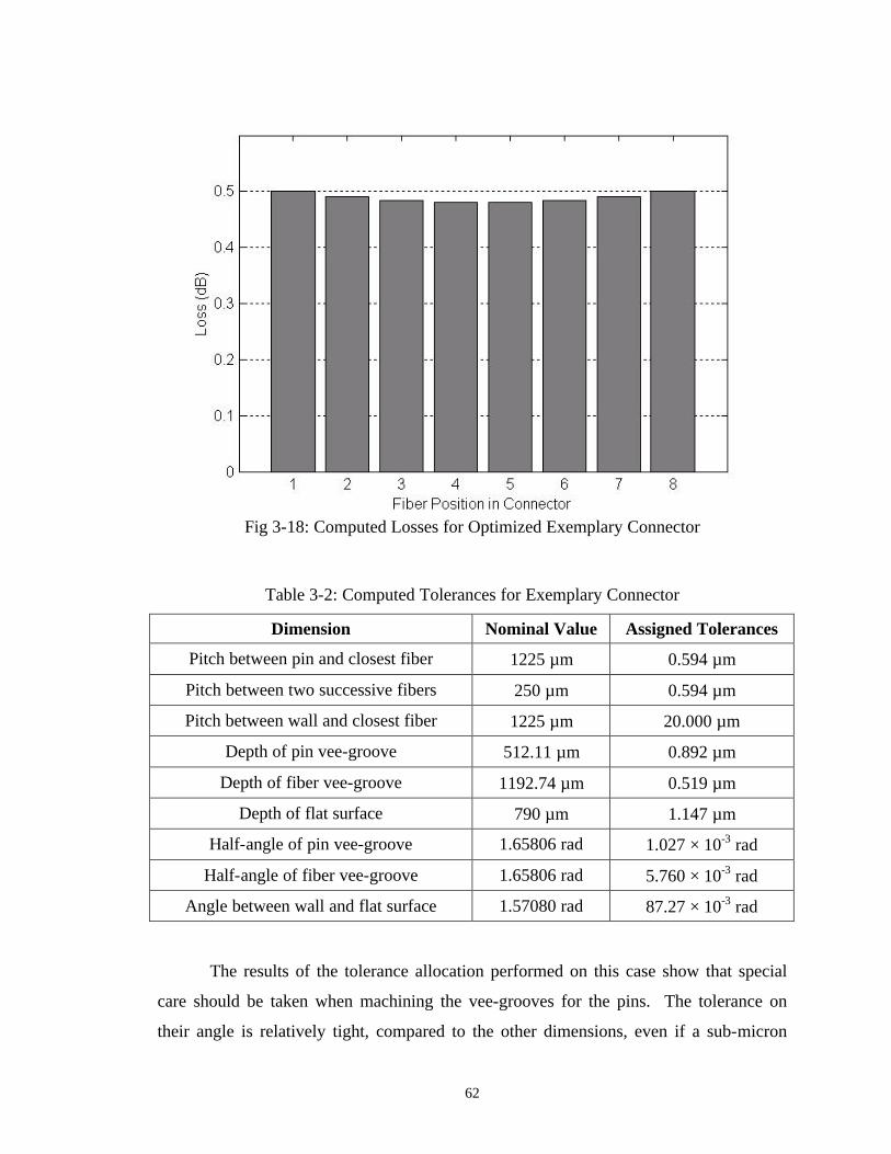
62

Fig 3-18: Computed Losses for Optimized Exemplary Connector

Table 3-2: Computed Tolerances for Exemplary Connector

Dimension Nominal Value Assigned Tolerances

Pitch between pin and closest fiber 1225 µm 0.594 µm

Pitch between two successive fibers 250 µm 0.594 µm

Pitch between wall and closest fiber 1225 µm 20.000 µm

Depth of pin vee-groove 512.11 µm 0.892 µm

Depth of fiber vee-groove 1192.74 µm 0.519 µm

Depth of flat surface 790 µm 1.147 µm

Half-angle of pin vee-groove 1.65806 rad 1.027 × 10-3 rad

Half-angle of fiber vee-groove 1.65806 rad 5.760 × 10-3 rad

Angle between wall and flat surface 1.57080 rad 87.27 × 10-3 rad

The results of the tolerance allocation performed on this case show that special

care should be taken when machining the vee-grooves for the pins. The tolerance on

their angle is relatively tight, compared to the other dimensions, even if a sub-micron

63

tolerance is needed for most of the dimensions defining the ferrule. On the other hand,

tolerances related to the flat surface of the ferrules are relatively opened. The tolerance

allocation demonstrates that the manufacturing cost of the ferrule can be reduced when

making this geometric feature, since the flat surface doesn’t require the high level of

accuracy needed for the rest of the ferrule.

3.3.5. Comparison with Monte Carlo Simulation

Monte Carlo simulation, whose algorithm is presented in Fig 3-19, is used to

verify the results of the tolerance allocation. A large number of connectors with random

dimensions are virtually generated; then a statistic treatment of the results returns the

mean and standard deviation of the signal loss. These simulated data should be

comparable to the results obtained with the law of error propagation applied to the

parametric model of the connector.

Start

Generate a Random Connector

Quantity ofSamples?

Calculate Signal Loss dueto Lateral Misalignment

Record Signal Loss

Calculate Mean and StandardDeviation of Signal Loss

Display Mean andStandard Deviation of Loss

End

Input Nominal Dimensions andTolerances for Fibers

Input Nominal Dimensions andTolerances for Pins

Input Nominal Dimensions andTolerances for Ferrules

Fig 3-19: Flowchart of Monte Carlo Simulation for Multi-Fiber Connectors

64

Such Monte Carlo simulation is applied on the exemplary connector, with the

nominal dimensions and assigned tolerances presented in Table 3-2. The results are

displayed with a cumulative distribution function of the signal loss for every pair of

mating fibers, shown in Fig 3-20. As expected, every loss is less than 0.5 dB for 99.5%

of the cases with the selected set of tolerances.

Fig 3-20: Monte Carlo Simulation for Exemplary Connector with Optimized Tolerances

3.4. Manufacturing Process

3.4.1. Introduction

Tolerancing the optical fiber connector leads to the study of their production

process. This section presents initial results from investigating the manufacture of high

precision micro-scale vee-grooves fabricated in Aluminum 6061-T6. The manufacturing

process being tested includes three primary steps. The first step produces the rough

shape of the vee-grooves using conventional wire electro discharge machining (wire

EDM). The second step coats the grooves with a hard layer using the Sandford process.

The final step will produce precise vee-grooves with smooth surfaces by grinding away a

65

portion of the hard coating. In this chapter, we describe the fabrication process, assess

the surfaces of the vee-grooves, and evaluate manufacturing variation in the form of the

vee-grooves prior to the grinding step. The recast layer and coating thickness were

investigated using metallography.

Micro grooves and channels can be manufactured with material removal

processes such as etching [43], mechanical cutting with miniature cutters [44,45], and

non-traditional micro machining [46]. Alternatively, they can be formed with processes

such as coining [47] and molding.

The objective in this work is to investigate the suitability of a process for

producing micro vee-grooves in aluminum 6061-T6 with processes and equipment that

are readily available. Etching processes are not readily available to most manufacturers

and are not appropriate for aluminum. Mechanical cutting, which is readily available,

produces burrs that are significant at this length scale [48] and are difficult to remove.

For these reasons, a process based on wire electro discharge machining (wire EDM) and

precision grinding is investigated. For testing purposes, the vee-grooves of the first

ferrule prototypes were manufactured with nominal width, depth, and aperture angles of

approximately 180 µm, 156 µm, and 60 degrees, respectively, after grinding.

3.4.2. Description of the Process

The first step in the manufacturing process is to cut the general shape of the vee-

grooves using conventional wire EDM. This process is applicable for any conductive

material, and many EDM machines are capable of using wires with diameters as small as

20 ìm. Wire EDM can therefore produce a wide variety of groove geometries with

lengths up to many millimeters. Unfortunately, wire EDM generates a recast layer

produced by the re-solidification of molten metal. This undesirable surface is clearly

visible with scanning electron microscopy (SEM) as shown in Fig 3-21. The imprecision

of the vee-grooves and the rough surface justify grinding after EDM.

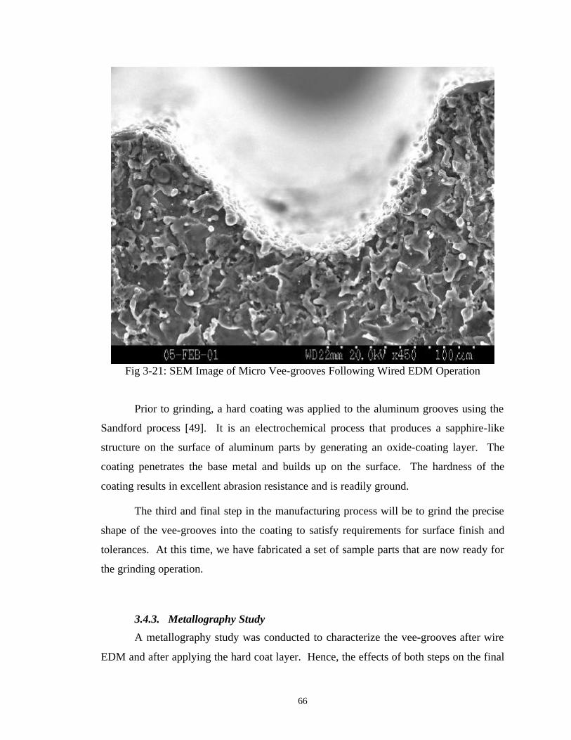
66

Fig 3-21: SEM Image of Micro Vee-grooves Following Wired EDM Operation

Prior to grinding, a hard coating was applied to the aluminum grooves using the

Sandford process [49]. It is an electrochemical process that produces a sapphire-like

structure on the surface of aluminum parts by generating an oxide-coating layer. The

coating penetrates the base metal and builds up on the surface. The hardness of the

coating results in excellent abrasion resistance and is readily ground.

The third and final step in the manufacturing process will be to grind the precise

shape of the vee-grooves into the coating to satisfy requirements for surface finish and

tolerances. At this time, we have fabricated a set of sample parts that are now ready for

the grinding operation.

3.4.3. Metallography Study

A metallography study was conducted to characterize the vee-grooves after wire

EDM and after applying the hard coat layer. Hence, the effects of both steps on the final

67

precision of the vee-grooves can be identified. The metallography study consisted of

slicing the manufactured parts, mounting the parts, grinding and polishing the parts’

endfaces, and finally observing the faces with an optical microscope.

A part cut with wire EDM but before coating was studied to characterize the

recast layer observed in Fig 3-21. The recast layer produced a generally rough profile

around the perimeter of the part that varied in thickness from between 4 ìm and 8 ìm as

shown in Fig 3-22.

6 µm

4 µm

6 µm

Aluminum

72

207 µm

97 µm

Fig 3-22: Metallography Study of a Vee-Groove Produced with Wire EDM

Fig 3-23 shows an image of a vee-groove after coating with the Sandford process.

The thickness of the coating layer was not uniform, and it varied with the geometry of the

vee-groove. On the sloped surfaces, the thickness was typically about 32 ìm thick, but

the thickness was only 16 ìm at the bottom of the grooves. A thicker coating layer is

achievable with a longer coating time, and may be necessary if gross errors exist during

grinding.

68

32 µm32 µm

16 µm

Aluminum

72

174 µm

112 µm

Fig 3-23: Metallographic Study of Coated Vee-Groove

3.4.4. Stylus Profilometry of Grooves

The accuracy and variation of the grooves’ 2D shape was assessed prior to

coating. Since the width, depth, and length of the grooves were approximately 170 ìm,

150 ìm, and 4 mm (before grinding), a 3D approach over the area of the grooves was

necessary. Stylus profilometry was selected as the measurement technique since it

provided suitable resolution in the z direction (~1 nm) over the necessary scan area (4

mm x 4.6 mm).

The stylus (~0.2 ìm diameter) traveled along a path in the horizontal plane and

recorded the height of the surface. The surface was scanned in a raster fashion by

measuring a set of parallel traces. Traces were sequentially measured across the set of

parallel grooves (x direction) with an increment in the y direction of 50 ìm. The scan

velocity in the x direction was 200 ìm/s, and it sampled the height of the surface at 1 ìm

intervals. Thus a 3D point cloud of data points was collected, and it is shown in Fig 3-24

along with the ideal geometry.

69

y

x

z

4.6 mm4.0 mm

Fig 3-24: Point Cloud from Profilometry Traces

The manufacturing variation in the vee-grooves is observed after projecting the

3D point cloud onto a 2D plane intersecting the parallel vee-grooves. In Fig 3-25, it is

evident that the EDM process did not remove the material at the very bottom of the

grooves.

Fig 3-25: 3D Profilometry Data Projected onto a 2D Plane for Comparison to Ideal

Model

70

As shown in Fig 3-26, the geometry of a vee-groove is represented in two

dimensions with four parameters and their manufacturing errors:

• angle of aperture, α, and angle error, jαδ ,

• inclination angle, γ, which is the angle between the groove’s bisector and a vertical

line (ideally γ �equals zero), and angle error, jγδ ,

• depth to the virtual vertex, h, and error, jhδ , and the

• radius of curvature, r, at the bottom of the groove, and error, jrδ .

Vertexx

z

0

jj αδα + jγδ

jhjh δ+jrjr δ+

Fig 3-26: Manufacturing Errors in a Vee-Groove

A simple algorithm that calculates the geometric parameters of the grooves from

the measured profilometer data was developed [50]. For each vee-groove in a 2D trace,

the algorithm fitted a straight line to the inclined edges and determined their slope and

intersection. Thus two half-angles for every groove were calculated: the left one, βL, and

the right one, βR. The angle of aperture was determined as the sum of the half angles.

The intersection of the two fitted lines gave the coordinates of the groove’s virtual vertex,

and so the depth of the groove, h, was determined. The inclination angle was calculated

as half the difference between βL and βR.

Using this algorithm on 40 traces and 16 grooves per trace yielded the geometric

parameters of 640 2D grooves. Statistics characterizing the mean and variation of the

parameters are shown in Table 3-3.

71

Table 3-3: Statistics of 2D Geometric Parameters Describing Vee-Groove Variation

FeatureTargetvalue

LowerLimit

EstimatedMean

UpperLimit

LowerLimit

EstimatedVariance

UpperLimit

Left half angle (degrees) 30.0 34.41 34.63 34.84 7.1 7.9 8.9Right half angle (degrees) 30.0 35.07 35.30 35.54 8.2 9.2 10.3

Aperture (degrees) 60.0 69.59 69.93 70.27 16.9 18.8 21.1Inclination (degrees) 0.0 -0.49 -0.34 -0.19 3.5 3.8 4.3

Height (microns) 150 130.9 131.4 131.8 25.7 28.6 32.0

Estimate of the Mean(95% Confidence Interval)

Estimate of the Variance(95% Confidence Interval)

3.4.5. Conclusions

This chapter introduced a manufacturing process to make micro-scale vee-

grooves in Aluminum 6061T6 and a metrology procedure to measure their dimensional

variation. Surface roughness and variation were found to be significant after EDM and

coating, and so grinding remains necessary. A metallography study showed that variation

in the thickness of the coating layer depended upon groove geometry. The thickness of

the coating in the depth of the groove was approximately half the thickness on the flat

surfaces.

Despite the dimensional variation after wire EDM and coating, the grooves are

acceptable for subsequent grinding operations. The results of the grinding operation will

be presented in future work.

72

Chapter 4: Application to Kinematic Couplings

4.1. Introduction

4.1.1. Presentation

Kinematic couplings, illustrated in Fig 4-1, are widely used for positioning one

rigid body with respect to another. Contact between a ball body and a groove body

occurs at six points, which is the minimum necessary for static equilibrium. Hence,

kinematic couplings exactly constrain [5] all six degrees of freedom without over-

constraint and are therefore extremely repeatable techniques for positioning two bodies

[51,52]. However, the relative position and orientation of the two bodies are not

necessarily accurate. Accuracy must be attained with either mechanical adjustments or

tight production tolerances, both of which increase the manufacturing cost of the

kinematic coupling.

Vee Groove

Vee Grooves

BallBody

GrooveBody

Fig 4-1: Three-Groove Kinematic Coupling

73

As kinematic couplings increasingly find applications in manufacturing, fixturing,

and material handling, it is necessary to consider the effect of inaccurate kinematic

couplings. For instance, Vallance and Slocum [4] described the use of kinematic

couplings for positioning pallets in flexible assembly systems. In this application,

kinematically coupled pallets are routinely exchanged at multiple machine stations, and

hence manufacturing errors in each pallet and station contribute to system-wide

manufacturing variation.

This chapter presents a method for allocating tolerances to the dimensions of

kinematic couplings so that variation in the position and orientation of kinematically

coupled bodies is less than a set of design constraints. The geometry of the contacting

surfaces is modeled using parametric functions of dimensions that include manufacturing

errors. The variation in the kinematic couplings’ position and orientation errors are

expressed as a function of the tolerances using a multivariate error analysis [26]. The

tolerances of the coupled bodies are related to manufacturing costs via cost/tolerance

relations for common processes (milling, drilling, grinding, etc.) published by Chase [10].

Finally, a constrained nonlinear optimization problem returns dimensional tolerances for

the kinematic coupling that minimize manufacturing costs but satisfy constraints on

variation in position and orientation.

4.1.2. Background and Prior Work

Kinematic couplings have been used in precision instruments for many years

[53,54], and their utility in precision machines is widely recognized [55]. In traditional

applications, often a single ball body and a single groove body are ever coupled together,

and so the principal functions of the kinematic coupling are:

• to minimize variation in the position and orientation of the ball body after removing

and replacing the ball body, and

• to minimize elastic deformation induced in the ball body due to excessive constraints.

The success of similar anti-distortion mountings and kinematic couplings with

regard to these two functions was studied and demonstrated by designers of precision

74

instruments and machines [2,3,56]. As a result, they found increasing application within

precision manufacturing equipment and processes [4,57,58]. For some of these

applications, multiple ball bodies are coupled with a single or several groove bodies.

This introduces system-level variation due to inaccurate production of the mating

surfaces within the kinematic coupling, which was described and analyzed by Vallance

[26]. To increase the accuracy of each coupling and thereby reduce the system-wide

variation, the dimensional variation within the set of ball and groove bodies must be

specified and controlled.

Limits on the dimensional variation within the ball and groove bodies can be

specified on drawings using standard techniques for dimensional and geometric

tolerances [7]. Early tolerancing research resulted in approaches for tolerance analysis

that predict the effect of multiple tolerances on the dimensions and geometry of

mechanical components [59,60]. The most common approaches use worst-case analyses

[61], root-sum-square (RSS) analyses [62], statistical techniques [63], or Monte Carlo

simulation [64]. More recent research extended tolerance analysis techniques to

assemblies of components [65,66], and some of these techniques are available in

tolerance analysis software and may even be integrated with CAD software [67].

Software for tolerance allocation [68], which is the inverse problem of assigning

values to the tolerances, is less available. Therefore, tolerance allocation is less common,

but it has been demonstrated for particular mechanical systems [69]. Tolerance

allocation often uses optimization techniques [70] that minimize cost [71,72] subject to

constraints on variation using cost-tolerance relations [73].

This chapter contributes a formulation and solution to tolerance allocation for

kinematic couplings, which compliments other analytical tools that assist during design

[3,74,75]. The technique for assigning tolerances is statistical, and it uses multivariate

error analysis [15] and nonlinear constrained optimization [76] to minimize cost. The

technique has been implemented and verified using a set of scripts that execute within

Matlab. An additional set of Matlab scripts verifies the results of the allocation using

random Monte Carlo simulations.

75

4.1.3. Tolerance Allocation

Rigorously allocating tolerances to the dimensions of kinematic couplings,

requires an algorithm that incorporates the four aspects described below.

• Describe the geometry and dimensional variation in a mathematical form. Both

bodies of the kinematic coupling should be represented parametrically, with respect to

their nominal dimensions and their dimensional errors. The contact points between the

two bodies are of primary interest for defining the assembly variations of the kinematic

coupling, so the parametric representation should concentrate on contacting surfaces in

terms of the dimension schemes for modeling the ball and groove bodies.

• Combine dimensional variation in the ball body and groove body to estimate

variation in the resting position and orientation of the ball body. The limits to

dimensional variation in the ball and groove bodies are defined by tolerances. When a

ball and groove body with particular dimensional errors are assembled together, the ball

body is positioned and oriented with errors in its resting position (xr, yr, zr, αr, βr, γr). A

relation between dimensional variation and variation in the resting position and

orientation is provided by multivariate error analysis. This approach requires a robust

method for determining the resting location of the ball body.

• Relate assembly variation to the performance requirements of the kinematic coupling.

The acceptable errors in the resting position and location are defined by the assembly

tolerances specified by the designer. If the designer uses error budgeting techniques [77],

then the limits on position and orientation errors associated with the kinematic coupling

are known. However, these limits are usually specified at operating points, where

manufacturing operations are performed, rather than at a reference coordinate system.

The performance of the kinematic coupling should therefore be assessed using variation

in the position and orientation of operating points.

• Relate dimensional tolerances to manufacturing costs. The objective of the tolerance

allocation is to minimize the manufacturing cost of the kinematic coupling, while

satisfying tolerances on the assembly errors. It is then necessary to establish cost-

tolerance functions relevant to the manufacturing operations used to produce the ball and

groove bodies.

76

These four aspects are incorporated into the algorithm illustrated in Fig 4-2. The

multivariate error analysis is an iterative process in which one dimension is perturbed at a

time. It returns the variation of the resting location and the manufacturing cost. This

process is nested in an optimization loop.

77

Start

Set of Tolerances asa Starting Guess

Generate the CorrespondingBall Body

Perturbate one Dimension

Generate the CorrespondingGroove Body

Pertubed AllDimensions?

Calculate Jacobianof the System

Calculate CovarianceMatrix [CE] for the Variation

in the Resting Location

Calculate Variation inResting Location

CalculateManufacturing Cost

Can the CostBe Reduced?

Select a New Setof Tolerances

Yes

Display OptimizedSet of Tolerances

No

End

Input Nominal Dimensions forBall Body and Groove Body

Calculate CovarianceMatrix of Dimensions [CD]

No

Yes

Input Constraints on RestingLocation Variation

Fig 4-2: Flowchart of the Tolerance Allocation for Kinematic Couplings

78

4.2. Mathematical Model

4.2.1. Parametric Representation of Contacting Surfaces

We require an analytical representation of the contacting surfaces within a

kinematic coupling containing manufacturing errors. A common style of kinematic

couplings uses three balls resting in three vee-grooves, as illustrated in Fig 4-1 [74], and

so we use the parametric equations for a sphere and flat surface. We distinguish six

spherical surfaces since the effective diameter of the ball near the contact point may be

slightly different due to out-of-roundness in the ball. The arrangement of the six

spherical and flat surfaces is illustrated in Fig 4-3. For computational purposes,

coordinate systems are attached to each surface. The 12 surfaces are described in

reference coordinate systems located at the coupling centroid of the ball body (BC) and

groove body (GC).

x

zy

yx

z

z

z

x

x

x

yy

y

yy

y

y

x

x

z

z

GrooveSurface 6

Ball 5Surface

GrooveSurface 5

Ball 2Surface

GrooveSurface 4

GrooveSurface 3

GrooveSurface 2

Ball 1Surface

Ball 3Surface

Ball 4Surface

Ball 6Surface

CouplingCentroid

GrooveSurface 1

Fig 4-3: Parametric Representation of Spherical and Flat Contacting Surfaces

79

When load is not critical, the contact between a spherical surface and a flat

surface is punctual. Every point contact suppresses a degree of freedom, thus the six

contacts fully constraint the two bodies of the kinematic coupling.

Eq (4-1) describes all points [iii BBB zyx ,, ] that lie within a spherical surface with

diameter, iBd , and center located by the position vector, [ ]z

BBCy

BBCx

BBC

BBC

iiiiPPPP ,,=

v.

The subscript, Bi, indicates that the points are associated with the ith spherical surface, and

the prescript, BC, denotes that the position vector is measured in the coordinate system

located at the centroid of a triangle defined by the centers of the three balls. The sub-

subscript, i, which indicates a particular contact surface, varies between 1 and 6.

1...6for 04

1)()()( 2222 ==−−+−+− idPzPyPx

iiiiiii Bz

BBC

By

BBC

Bx

BBC

B (4-1)

Eq (4-2) describes all points [iii FFF zyx ,, ] that lie within the flat plane in one of

the coupling’s vee-grooves. The subscript, Fi, indicates that the variables are associated

with the ith flat surface. The plane is defined by a position vector that locates a point in

the vee-groove, [ ]zF

GCyF

GCxF

GCF

GCiiii

PPPP ,,=v

, and a vector normal to the plane,

[ ]zF

GCyF

GCxF

GCF

GCiiii

nnnn ,,=v. The prescript, GC, indicates that the vectors are

measured in a coordinate system located at the grooves’ coupling centroid.

1...6for 0)()()( ==−+−+− iPznPynPxn zF

GCF

zF

GCyF

GCF

yF

GCxF

GCF

xF

GC

iiiiiiiii (4-2)

The components of the position and normal vectors used in Eqs (4-1)-(4-2)

depend upon the manufactured dimensions of the kinematic coupling. Two sets of

dimensions, ( )mBBB ddd ,,,

21K and ( )

nFFF ddd ,,,21

K , define the geometry of the ball

body and groove body, respectively. The dimensions are measured with respect to two

sets of metrology datum frames that define a coordinate system in the ball body denoted

with a prescript, BD, and a coordinate system in the groove body denoted with a

prescript, GD. The form of these relations depends upon the dimension scheme specified

by the designer, but they are expressed generally as shown in Eqs (4-3)-(4-5).

80

( )mii BBBBB

BD dddfP ,,,21

Kv

= (4-3)

( )nii FFFFF

GD dddfP ,,,21

Kv

= (4-4)

( )nii FFFnF

GD dddfn ,,,21

Kv = (4-5)

The position vectors that locate the spherical and flat surfaces are transformed

from the coordinate systems determined by the manufacturing datums (BD and GD) to

the centroidal coordinate systems (BC and GC) using homogeneous transformation

matrices (HTMs), TBCBD and TGC

GD , as shown in Eqs (4-6)-(4-7).

ii BBDBC

BDBBC PTP

vv= (4-6)

ii FGDGC

GDFGC PTP

vv= (4-7)

The HTMs TBCBD and TGC

GD are determined using a triangle defined by the centers

of the balls. The origin of the centroidal coordinate system is located at the intersection

of the triangle’s bisectors [1]. Its x-axis points towards the ball that contains contacting

surfaces 5 and 6, and the three apices lie in the xy-plane. An algorithm for determining

TBCBD and TGC

GD is presented in Appendix E.

4.2.2. Resting Position and Orientation

When rigid ball and groove bodies are kinematically coupled, the ball body rests

in a location that minimizes energy. If friction at the contact points is neglected, the

resting location is determined solely from the manufactured geometry of the bodies. The

solution described here [26] uses the geometric model presented in the previous section

to calculate the relative position and orientation between kinematically coupled bodies

that contain manufacturing errors. By avoiding assumptions such as a linear relation

between manufacturing errors and resting position, the method remains valid for even

large manufacturing errors.

81

Specification of the resting position and orientation requires that three translations

xr, yr, and zr, and three rotations αr=rot(BCZ), βr=rot(BCY), and γr=rot(BCX) be determined.

These degrees of freedom are expressed in a transformation matrix, TGCBC , between the

centroid coordinate systems in the ball body (BC) and groove body (GC). The objective

is to determine the unknowns (xr, yr, zr, αr, βr, γr) and hence TGCBC , but this cannot be done

without also determining the position vectors that locate the six contact points, iC

GC Pv

.

Known Variables

6

5

4

3

2

1

B

B

B

B

B

B

d

d

d

d

d

d

6

5

4

3

2

1

BBC

BBC

BBC

BBC

BBC

BBC

P

P

P

P

P

P

v

v

v

v

v

v

6

5

4

3

2

1

FGC

FGC

FGC

FGC

FGC

FGC

P

P

P

P

P

P

v

v

v

v

v

v

6

5

4

3

2

1

FGC

FGC

FGC

FGC

FGC

FGC

n

n

n

n

n

n

v

v

v

v

v

v

System of 24Equations

NonlinearEquation

Solver

Unknown Variables

r

r

r

r

r

r

z

y

x

γβα

6

5

4

3

2

1

CGC

CGC

CGC

CGC

CGC

CGC

P

P

P

P

P

P

v

v

v

v

v

v

Fig 4-4: Solution for Resting Position and Orientation

As illustrated in Fig 4-4: , the solution employs a system of 24 equations and

unknowns that are solved iteratively using a nonlinear numerical technique. The inputs

to the solver include the diameters of the spherical contacting surfaces, iBd , the position

vectors that locate the balls in the BC coordinates, iB

BC Pv

, the position vectors that locate

the flat surfaces in the GC coordinates, iF

GC Pv

, and the normal vectors at the flat surfaces,

82

iFGCn

v. The outputs of the algorithm include the translations and rotations of the resting

position, xr, yr, zr, αr, βr, γr and the positions vectors that locate the six contact points in

the GC coordinate system, iC

GC Pv

.

The system of 24 equations is obtained in two distinct sets. The first set of six

equations is obtained by requiring that the contact points lie in the plane defined by the

flat surfaces. As shown in Eq (4-8), this is accomplished by substituting the coordinates

of the contact points into Eq (4-2), which may be done six times for each contact point.

1...6for 0)()()( ==−+−+− iPznPynPxn zF

GCC

zF

GCyF

GCC

yF

GCxF

GCC

xF

GC

iiiiiiiii (4-8)

The second set of eighteen equations is obtained from six equations that express a

closed loop of vectors between the contacting balls and flat surfaces. The vector loop is

illustrated in Fig 4-5 for one ball and flat surface. One path in the loop originates at the

GC coordinate system and includes the unknown transformation, TGCBC , and the position

of the ball center, iB

BC Pv

. The second path in the loop also originates at the GC

coordinate system, but it proceeds to the unknown position of the contact point, iC

GC Pv

,

and through a vector normal to the flat surface of magnitude 2/iBd . The closed vector

loop is expressed mathematically in Eq (4-9), and may be written six times for each

contact point.

1...6for 2

1 ==− ind

PPTiii F

GCBC

GCB

BCGCBC

vvv (4-9)

83

iFGC n

v

iCGC P

v

iBBC P

v

iFGC P

vB

BC y

x

z

GC

F

TGCBC

iBGC P

v

z

x

y

x

z

y

x

y

z

Fig 4-5: Vector Loop Between Ball and Flat Surface

After the iterative solver returns values for the unknown variables, the HTM

between the GC and BC coordinate systems is computed as shown in Eq (4-10). If the

rotations are small, then the matrix form may be simplified using small angles

approximations.

( ) ( ) ( ) ( ) ( ) ( ) ( ) ( ) ( ) ( ) ( ) ( )( ) ( ) ( ) ( ) ( ) ( ) ( ) ( ) ( ) ( ) ( ) ( )

( ) ( ) ( ) ( ) ( )

−−−−−

=

1000

coscossincossin

sincoscossinsincoscossinsinsincossin

sinsincossincoscossinsinsincoscoscos

rrrrrr

rrrrrrrrrrrrr

rrrrrrrrrrrrr

GCBC z

y

x

Tγβγββ

γαγβαγαγβαβαγαγβαγαγβαβα

(4-10)

4.2.3. Multivariate Error Analysis of Variation in Resting Location

Tolerance allocation requires a relation between dimensional variation and

system-wide variability in the resting position and orientation. This can be accomplished

using a Monte Carlo simulation, but multivariate error analysis provides a more

computationally efficient approach [26]. After allocating tolerances, a Monte Carlo

simulation is an effective means for verifying the results.

Multivariate error analyses use linear approximations derived from Taylor series

expansion. For instance, there exists a function, ),,( 21 dX +

84

As shown in Eq (4-11), an estimate of the deviation in the x-coordinate, rxδ , is

expressed using a Taylor series expansion to X that includes only first-order terms

consisting of partial derivatives and differential errors in the dimensions, jd∆ .

nmnmx d

Xd

d

Xd

d

Xd

r

++ ∂

∂∆++

∂∂

∆+∂∂

∆≈ ...2

21

1δ (4-11)

Similar expressions are written for the deviations in the remaining degrees of

freedom, ryδ ,

rzδ , rγδ ,

rβδ and rαδ . All six approximations are expressed in matrix form

by the transformation shown in Eq (4-12). The )(6 nm +× matrix of partial derivatives

is referred to as the Jacobian matrix, [J].

∆

∆∆

∂Α∂

∂Α∂

∂Α∂

∂Β∂

∂Β∂

∂Β∂

∂Γ∂

∂Γ∂

∂Γ∂

∂∂

∂∂

∂∂

∂∂

∂∂

∂∂

∂∂

∂∂

∂∂

=

+

+

+

+

+

+

+

nm

nm

nm

nm

nm

nm

nm

z

y

x

d

d

d

ddd

ddd

ddd

d

Z

d

Z

d

Zd

Y

d

Y

d

Yd

X

d

X

d

X

r

r

r

r

r

r

M2

1

21

21

21

21

21

21

...

...

...

...

...

...

α

β

γ

δδδδδδ

(4-12)

Since expressions for the six degrees of freedom are not actually known, the

elements of [J] are estimated numerically. This is done by perturbing the value of each

dimension from its nominal value, calculating the resting location that gives the six

errors, and then evaluating a column in [J].

Assuming the dimensions are continuously distributed random variables and that

a tolerance is equivalent to a 3σ range, the error analysis can be treated statistically. A

covariance matrix organizes variances along its diagonal and covariances in the off-

diagonal terms. The diagonal elements are therefore squares of the standard deviations of

the corresponding random variables. The covariance matrix, [CD], of the kinematic

coupling's dimensions is given in Eq (4-13). If the dimensions are independent and

85

therefore uncorrelated, the off-diagonal covariance terms will equal zero. This is a

common assumption during tolerance allocation.

[ ]

( ) ( )( ) ( )

( ) ( )

=

+++

+

+

221

22

12

1212

,cov,cov

,cov,cov

,cov,cov

2

1

nmdnmnm

nmd

nmd

D

dddd

dddd

dddd

C

σ

σσ

L

MOMM

L

L

(4-13)

A similar covariance matrix, [CE], for the variation in the resting location is

defined in Eq (4-14).

[ ]

( ) ( )( ) ( )

( ) ( )

=

2

2

2

,cov,cov

,cov,cov

,cov,cov

r

r

r

rrrr

rryrr

rrrrx

E

yx

yxy

xyx

C

ασαα

ασασ

L

MOMM

L

L

(4-14)

The covariance matrix of the resting location errors, [CE], is related to the

covariance matrix of the dimensions [CD] by Eq (4-15) [15].

[ ] [ ][ ][ ]TDE JCJC = (4-15)

By extracting the diagonal elements of the matrix, [CE], the multivariate error

analysis returns the variation in the resting position and orientation in terms of the

tolerances on dimensions.

4.2.4. Variation at Operating Points

The previous section presented a method for estimating the variation in the

position and orientation of a coordinate system located at the coupling centroid in the ball

body. Although this is useful, the utility of the tolerance allocation is greatly improved if

it considers the variation at additional points in the ball body. For instance, in kinematic

couplings intended for positioning pallets in flexible assembly operations [4], assembly

operations such as insertion and joining are performed to a product held within a fixture

attached to the ball body. Hence, the designer’s specifications on variation, as

determined with an error budget, are preferably specified at operating points.

86

Fig 4-6 illustrates the definition of a single operating point. A coordinate system,

denoted with the prescript, OPk, is defined at the kth operation point. An HTM, TBDOPk

,

locates the operating point with respect to the manufacturing datum frame in the ball

body, BD. A set of p operating points is similarly defined by a set of p HTMs.

GC x

yz

x

yz

OperatingPoint

TkOPGC

x

yz

BD TkOPBD

TGCBD

OPk

Fig 4-6: Coupled Kinematic Coupling with Operating Point

After determining TBCBD between the ball body’s datums and coupling centroid

using the algorithm in Appendix E, the position and orientation of the operating points

can be calculated in the coordinate system at the groove body’s coupling centroid using

the transformations shown in Eq (4-16). Since TGCBC contains the resting position errors

resulting from coupling the ball and groove bodies, the transformation TGCOPk

reveals the

effect of an inaccurate coupling on the position and orientation at the operating point.

Larger position errors usually result from amplifying small rotations by the distance

separating the operating point from the coupling centroid (Abbe offset).

87

TTTT BDOP

BCBD

GCBC

GCOP kk

= (4-16)

The multivariate error analysis is expanded to include the operating points. This

is accomplished by expanding the vector of errors and the Jacobian matrix as shown in

Eq (4-17) so that they incorporate error terms associated with the set of p operating

points. If all six degrees of freedom at each operating point are included, then the

dimensions of the error vector become (6+6×p)×1, and the dimensions of the Jacobian

matrix become (6+6×p)×(m+n). However, most manufacturing operations have sensitive

and insensitive directions, so considering only the sensitive directions simplifies the

problem and requires only a subset of the degrees of freedom at each operating point.

Evaluation of the new terms in the Jacobian matrix is still determined by perturbing each

dimension in the ball and groove body, calculating the resting position and orientation,

and subsequently extracting changes in the values within TGCOPk

.

∆

∆∆

∂

Α∂

∂

Α∂

∂

Α∂

∂∂

∂∂

∂∂

∂∂

∂∂

∂∂

=

+

+

+

+

nm

nm

OPOPOP

nm

rrr

nm

rrr

y

x

z

y

x

d

d

d

ddd

d

Y

d

Y

d

Yd

X

d

X

d

X

ppp

pOP

OP

OP

r

r

r

r

r

r

M

L

MOMM

L

L

M

2

1

21

21

21

1

1

α

α

β

γ

δ

δδδδδδδδ

(4-17)

With the changes shown in Eq (4-17), the covariance matrix [CE] calculated with

Eq (4-15) takes the alternative form shown in Eq (4-18). This form includes additional

terms for the variances and covariances associated with the position and orientation at the

operating points.

88

[ ]

( ) ( ) ( )( ) ( ) ( )

( ) ( ) ( )

( ) ( ) ( )

=

2

2

2

2

,cov,cov,cov

,cov,cov,cov

,cov,cov,cov

,cov,cov,cov

pOPkppp

pkkOPkk

pkr

pkr

OPOPrOPrOP

OPOPxrOPrOP

OPrOPryrr

OPrOPrrrx

E

xyx

xyxxx

yxyxy

xxxyx

C

ασααα

ασ

ασ

ασ

LL

MOMMMM

LL

MLMOMM

LL

LL

(4-18)

4.3. Tolerance Allocation

4.3.1. Manufacturing Cost and Tolerances

The cost of manufactured ball and groove bodies depends upon the selected

manufacturing process and dimensional tolerances. The cost of achieving a particular

tolerance depends upon both the dimension's nominal value and its tolerance. The

manufacturing cost generally increases if the tolerance is tightened, and it is more

expensive to hold a given tolerance on larger nominal dimensions. Based on this, Chase

[10] recommends expressing tolerances as reciprocal power functions. Eq (4-19)

expresses the tolerance for the jth dimension, tj, as a function of cost, Cj, range, Rj, and

three constants aj, bj, and cj. The values of the three constants depend upon the range and

the manufacturing process. Although a constant term in Eq (4-19) would be necessary

for accuracy, it is practically impossible to evaluate and doesn’t affect the tolerance

allocation.

j

j

bj

aj

jjC

Rct ×= (4-19)

Chase provides a set of cost-tolerance curves for some metal removal processes

[10]. By extrapolating these curves, we determine values for the coefficients aj, bj and cj

for each dimension in the kinematic coupling. Table 4-1 presents the coefficients

calculated for an exemplary kinematic coupling configuration.

89

Table 4-1: Coefficients for Cost / Tolerance Relations

Dimension Process aj bj cj

Thickness of the plate Milling 0.4431 2.348 0.0355

Length of a leg Grinding 0.4323 1.385 0.0217

Diameter of a ball Lapping 0.3862 1.052 0.0130

Location of a hole Milling 0.4431 2.257 0.0255

Height of a vee-groove Grinding 0.4323 1.421 0.0228

Using the values in Table 4-1, Eq (4-19) defines the manufacturing cost for every

dimension in the exemplary kinematic coupling. Plots of the relations in Fig 4-7

illustrate the effect of tightening tolerances. The portion of the total manufacturing cost

that is attributable to tolerancing is then the sum of the costs for all l dimensions in the

ball and groove bodies, as shown in Eq (4-20).

jj bl

j j

ajj

total t

RcC

1

1∑

=

⋅= (4-20)

l being the number of manufacturing processes.

90

Fig 4-7: Cost / Tolerance Relations for Dimensions

4.3.2. Tolerance Allocation by Optimization

Optimal tolerances for the dimensions are determined using nonlinear constrained

optimization. The problem is formulated as shown in Eq (4-21), where the total cost

from Eq (4-20) is used as the objective function that is minimized. Constraints are

formulated by specifying that the standard deviation of the translation and rotation errors

must be positive yet below critical values. Additional bounds can be specified to prevent

the optimization from driving the assigned tolerances to unreasonably high or low values.

91

that such minimize1

/1

⋅∑

=

l

j

b

j

ajj

jj

t

Rc

max

max

max

max

max

max

0

0

0

0

0

0

rr

rr

rr

rr

rr

rr

zz

yy

xx

γγ

ββ

αα

σσ

σσ

σσ

σσ

σσ

σσ

≤≤

≤≤

≤≤

≤≤

≤≤

≤≤

(4-21)

The allocation method was used to allocate tolerances to an exemplary kinematic

coupling. The parametric surface representation was based on 25 dimensions in the ball

body (m=25) and 18 dimensions (n=18) in the groove body, illustrated in Fig 4-8 and Fig

4-9. Some dimensions may look redundant, but they are actually needed to express the

purely geometric tolerances in terms of dimensional tolerances. The cost-tolerance

coefficients listed in Table 4-1 and the constraints listed in Table 4-2 were used during

the optimization. The resulting tolerances allocated by the optimization procedure are

listed in Table 4-3. The different Matlab codes are presented in Appendix D.

92

Ay

Ax

Az

6.35

19.05

19.05

19.05

Ø 12.70

Ø 12.70

Ø 12.70

25.40

25.40

177.80

25.40

101.60

177.80

Fig 4-8: Dimension Schemes for the Ball Pallet, in its Datum Frame

Ay

Ax

π/3

-π/3

Ay

Az

2.54

2.54

2.54

π/4

π/4

25.40

25.40

177.80

25.40

101.60

177.80

Fig 4-9: Dimension Schemes for the Groove Body, in its Datum Frame

93

Table 4-2: Constraints Used for Exemplary Tolerance Allocation

Variation Constraint Calculated max

rxσ 6.67 µm 5.23 µm max

ryσ 6.67 µm 6.67 µm max

rzσ 6.67 µm 4.87 µm max

rγσ 1.164×10-3 rad 0.115×10-3 rad max

rβσ 1.164×10-3 rad 0.068×10-3 rad max

rασ 1.164×10-3 rad 0.078×10-3 rad

Table 4-3: Computed Tolerances

Dimensions Nominal

Dimension Assigned Tolerance

Thickness of the plate 6.35 mm 1.000 mm Length of a leg (×3) 19.05 mm 0.749 mm Ball diameter (×3) 12.70 mm 0.464 mm

Roundness of ball at contact point (×6) 0 mm 0.071 mm Leg 1 25.40 mm Leg 2 25.40 mm

X coordinate of a leg-axis at the top of the plate

Leg 3 177.80 mm 0.030 mm

Leg 1 177.80 mm Leg 2 25.40 mm

Y coordinate of a leg-axis at the top of the plate

Leg 3 101.6 mm 0.030 mm

Leg 1 25.40 mm Leg 2 25.40 mm

X coordinate of a leg-axis at the bottom of the plate

Leg 3 177.80 mm 0.030 mm

Leg 1 177.80 mm Leg 2 25.40 mm

Bal

l Pal

let

Y coordinate of a leg axis at the bottom of the plate

Leg 3 101.6 mm 0.030 mm

Height of the vertices for the groove body (×3) 2.54 mm 0.449 mm Groove 1 -π/3 rad

Groove 2 π/3 rad Orientation angle of a groove Groove 3 π rad

0.100 rad

Half-angle of aperture of a groove (×6) π/4 rad 0.078 rad Groove 1 25.40 mm Groove 2 25.40 mm X coordinate of a groove Groove 3 177.80 mm

0.419 mm

Groove 1 177.80 mm Groove 2 25.40 mm

Gro

ove

Bod

y

Y coordinate of a groove Groove 3 101.60 mm

0.419 mm

Total number of dimensions: 43

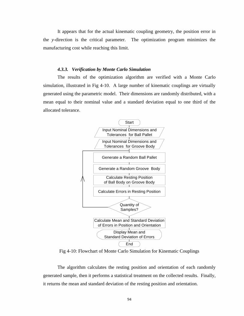
94

It appears that for the actual kinematic coupling geometry, the position error in

the y-direction is the critical parameter. The optimization program minimizes the

manufacturing cost while reaching this limit.

4.3.3. Verification by Monte Carlo Simulation

The results of the optimization algorithm are verified with a Monte Carlo

simulation, illustrated in Fig 4-10. A large number of kinematic couplings are virtually

generated using the parametric model. Their dimensions are randomly distributed, with a

mean equal to their nominal value and a standard deviation equal to one third of the

allocated tolerance.

Start

Generate a Random Ball Pallet

Generate a Random Groove Body

Quantity ofSamples?

Calculate Resting Positionof Ball Body on Groove Body

Calculate Errors in Resting Position

Calculate Mean and Standard Deviationof Errors in Position and Orientation

Display Mean andStandard Deviation of Errors

End

Input Nominal Dimensions andTolerances for Groove Body

Input Nominal Dimensions andTolerances for Ball Pallet

Fig 4-10: Flowchart of Monte Carlo Simulation for Kinematic Couplings

The algorithm calculates the resting position and orientation of each randomly

generated sample, then it performs a statistical treatment on the collected results. Finally,

it returns the mean and standard deviation of the resting position and orientation.

95

Table 4-4 compares the results computed by the optimization algorithm with

those calculated by the Monte Carlo simulation. The inputs were the nominal dimensions

and the assigned tolerances presented in Table 4-3. 10,000 samples were generated for

the simulation. For a better comparison, the limits of a 95% confidence interval were

computed on the standard deviations of the six errors returned by the simulation.

Table 4-4: Comparison Optimization / Simulation

Simulation: Limits of the 95% confidence interval Standard Deviation

Results of Tolerance Allocation Lower Upper

rxσ (µm) 5.23 5.14 5.28

ryσ (µm) 6.67 6.66 6.85

rzσ (µm) 4.87 4.81 4.94

rγσ (× 10-6 rad) 115 114 117

rβσ (× 10-6 rad) 67.5 66.1 67.9

rασ (× 10-6 rad) 78.4 76.6 78.7

4.4. Conclusion

Kinematic couplings are known as an economical method for precisely locating

one body with respect to another, but the relative position and orientation between the

coupled bodies depends upon manufacturing errors. In systems that exchange coupled

bodies, system-wide variation results from the inaccuracy of dimensions in each body.

Therefore, tolerances should be selected so that the system-wide variation is within a

specified range.

This chapter presents and demonstrates a method for allocating tolerances to the

dimensions of the bodies. A parametric representation of the contacting surfaces is

constructed and combined with a procedure that calculates the resting location based on

the inaccurate dimensions. An analytical relation between dimensional variation and

variation in the resting location is obtained from multivariate error analysis. Optimal

tolerances are computed by minimizing the relative manufacturing cost while respecting

constraints on variation in the resting position and orientation.

96

Chapter 5: Conclusions and Future Work

5.1. Conclusions

Exactly constrained systems present interesting characteristics for precision

engineering. In effect, they are repeatable, economical to build, and predictable if used

advisedly. These properties suggest that it is possible to combine them in order to reduce

the manufacturing cost of mass-produced kinematic systems. This thesis verified this

hypothesis by developing a rigorous procedure for solving the current problem; then it

illustrated the resulting method with two relevant examples.

The cost and the performances of a mechanical assembly are governed by the

tolerances assigned to the dimensions and the geometry of the components. That is the

reason why the developed procedure was a least cost tolerance allocation. A

mathematical model is established for the exactly constrained system by a comprehensive

analysis of its kinematic connections. The manufacturing variations are combined by

applying principles of statistics similar to the ones used in the SPC method; the

developed procedure could then be easily incorporated in a quality policy. A basic study

of the functional requirements of the system enables the establishment of a direct relation

between its performances and its manufacturing variations. Finally, empirical functions

established from experimental observations relate variation and cost in manufacturing.

These different analyses are nested in an optimization algorithm in order to perform a

least cost tolerance allocation.

In conclusion, this thesis presents an analytical tool for the precision design

engineer. It helps him or her to select the tolerances to assign to a kinematic system in

order to reduce its manufacturing cost while respecting its functionality. The developed

method enables the use of the efficiency of precision engineering for solving a current

industrial problem.

5.2. Future Work

The presented method is ready to be used, which is proven by the two performed

examples. However, it can be improved. First of all, other methods for analyzing the

97

variations can be explored in addition to the ones presented in Section 2.2.3. They may

be more suitable for other kinematic configurations. Some promising methods are

described in literature dealing with optimization problems in general [12]; they can be

adapted for least cost tolerance allocation procedures.

Furthermore, new cost / tolerance relations can be experimentally established for

manufacturing processes different from the traditional metal removal processes. In

effect, the existing relations only deal with these kinds of processes. Other processes like

etching, EDM, or LIGA technique can be used to produce exactly constrained

components, especially in a precision engineering field. Hence it would be interesting to

establish their cost / tolerance relations in order to extend the possibility of the current

method.

On the other hand, the presented method reduces the manufacturing cost only by

assigning the tolerances. A broader analysis could also optimize the nominal values of

the dimensions. This improved method would not only be a least cost tolerance

allocation, but a more global design optimization procedure that would be more efficient

for reducing the manufacturing cost of the mass-produced components.

Finally, the robustness of the current method can be improved by taking into

consideration the effects of mechanical loads, vibrations, and similar constraints. In

effect, the presented procedure assumed that these external mechanical disturbances were

negligible. Incorporating them into the least cost optimization method would then widen

the scope of the analysis. These disturbances would be expressed as additional

constraints in the optimization algorithm, since they characterize the performance of the

system.

98

Appendix A:

Probability Density Function of Sum of Squares

Problem statement:

X: Gaussian random variable X ~ N(0, σX)

Y: Gaussian random variable Y ~ N(0, σY)

X and Y are independent.

What is the probability density function of 22 YXR += ?

Joint density function of X and Y:

+−×

⋅⋅=

2

2

2

2

2

1exp

2

1),(

YXYXXY

yxyxf

σσσσπ (A1)

Let X = R cos θ and Y = R sin θ

Jacobian of the transformation:

( ) RRRRYX

R

Y

R

X

J =+=−

=

∂∂

∂∂

∂∂

∂∂

= θθθθ

θθ

θθ

22 sincoscossin

sincos (A2)

JyxfRf XYR ×= ),(),( θθ (A3)

+−×

⋅⋅=⇔

2

2

2

22 sincos

2exp

2),(

YXYXR

RRRf

σθ

σθ

σσπθθ (A4)

⋅

−+−×

⋅⋅=⇔ θ

σσσσ

σσσπθθ

222

22

2

2

cos1

2exp

2),(

YX

XY

YYXR

RRRf (A5)

99

⋅

⋅−

⋅−×⋅⋅

−×

=⇔ θσσσσ

σσπσ

θθ2

22

2222

2

cos2

exp2

2exp

),(YX

XY

YX

YR

R

RR

Rf (A6)

Probability density function of R:

θθπ

θ dRfRf RR ⋅= ∫ ),()(2

0

(A7)

tconsRR Rftan

),(=

θθ is a π-periodical even function, so:

θθπ

θ dRfRf RR ⋅= ∫ ),(4)(2

0

(A8)

θθσσσσ

σσπσ

π

dR

RR

RfYX

XY

YX

YR ⋅

⋅

⋅−

⋅−×⋅⋅

−×

=⇔ ∫2

0

222

2222

2

cos2

exp2

exp2

)( (A9)

Change of variables: let θcos=z zarccos=⇔ θ

Derivation: 21 z

dzd

−−=θ

Limits: if 0=θ then 1=z

if 2

πθ = then 0=z

dzzR

z

RR

RfYX

XY

YX

YR ⋅

⋅

⋅−

⋅−⋅−

×⋅⋅

−×

=⇔ ∫1

0

222

222

2

2

2

2exp

1

12exp2

)(σσσσ

σσπσ

(A10)

100

Note:

×

−=

−

⋅−∫ 2

,02

exp21

)exp(1

02

2 ABesselI

Adx

x

xA π, A being a constant and

BesselI(v, x) being a function that satisfies the modified Bessel equation:

0)('" 222 =⋅+−⋅+⋅ yvxyxyx

Then:

⋅

−⋅×

⋅

−⋅−×

⋅

−×

= 22

222

22

2222

2

4,0

4exp

2exp

)(YX

XY

YX

XY

YX

YR

RBesselI

R

RR

Rfσσσσ

σσσσ

σσσ

(A11)

⋅

−⋅×

⋅⋅+⋅

−×⋅

=⇔22

222

22

222

4,0

4

)(exp)(

YX

XY

YX

YX

YXR

RBesselI

RRRf

σσσσ

σσσσ

σσ (A12)

101

Appendix B:

Matlab Codes for Kinematic Couplings

B1. Optimization: Objective Function function f = kct_obj(x) % COEFFICIENTS % Coefficients CA CA_lap = 0.3862; CA_grind = 0.4323; CA_ream = 0.2880; CA_mill = 0.4431; CA_turn = 0.3515; % It will be CA-1 for the angles % Ranges R R_Thick = 6.35; R_Length = 19.05; R_Diam = 12.70; R_Circ = R_Diam; R_PosB = 177.8; % X and Y should have the same tolerance R_Height = 31.75; % Hypothenuse R_Orient = 38.1; R_Halfa = R_Height; R_PosG = 177.8; % X and Y should have the same tolerance % Coefficients CB CB_Thick = 2.3480; CB_Length = 1.3847; CB_Diam = 1.0516; CB_Circ = CB_Diam; CB_PosB = 2.2568; CB_Height = 1.4207; CB_Orient = 1.3490; CB_Halfa = CB_Height; CB_PosG = 2.2568; % Coefficients Bm Bm_Thick = 0.3420; Bm_Length = 0.1578; Bm_Diam = 0.0410; Bm_Circ = Bm_Diam; Bm_PosB = 0.5440;

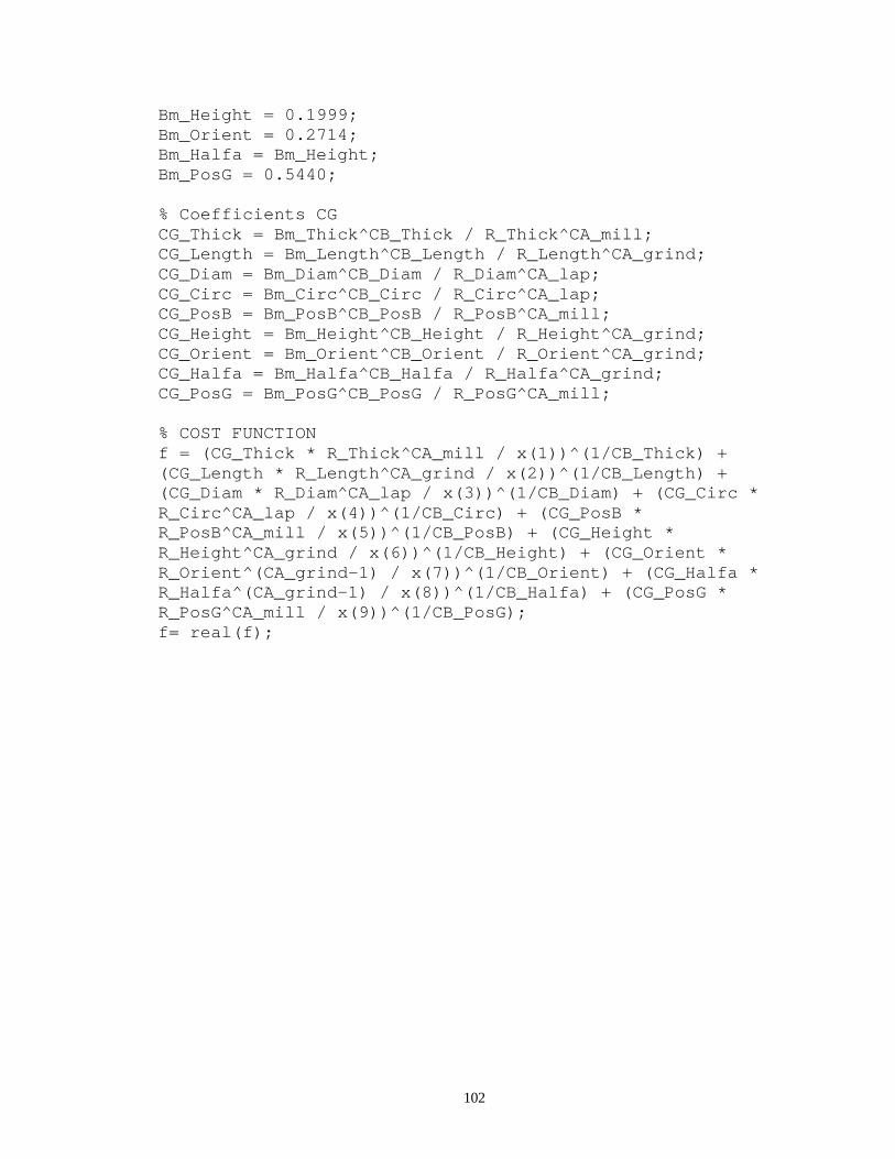
102

Bm_Height = 0.1999; Bm_Orient = 0.2714; Bm_Halfa = Bm_Height; Bm_PosG = 0.5440; % Coefficients CG CG_Thick = Bm_Thick^CB_Thick / R_Thick^CA_mill; CG_Length = Bm_Length^CB_Length / R_Length^CA_grind; CG_Diam = Bm_Diam^CB_Diam / R_Diam^CA_lap; CG_Circ = Bm_Circ^CB_Circ / R_Circ^CA_lap; CG_PosB = Bm_PosB^CB_PosB / R_PosB^CA_mill; CG_Height = Bm_Height^CB_Height / R_Height^CA_grind; CG_Orient = Bm_Orient^CB_Orient / R_Orient^CA_grind; CG_Halfa = Bm_Halfa^CB_Halfa / R_Halfa^CA_grind; CG_PosG = Bm_PosG^CB_PosG / R_PosG^CA_mill; % COST FUNCTION f = (CG_Thick * R_Thick^CA_mill / x(1))^(1/CB_Thick) + (CG_Length * R_Length^CA_grind / x(2))^(1/CB_Length) + (CG_Diam * R_Diam^CA_lap / x(3))^(1/CB_Diam) + (CG_Circ * R_Circ^CA_lap / x(4))^(1/CB_Circ) + (CG_PosB * R_PosB^CA_mill / x(5))^(1/CB_PosB) + (CG_Height * R_Height^CA_grind / x(6))^(1/CB_Height) + (CG_Orient * R_Orient^(CA_grind-1) / x(7))^(1/CB_Orient) + (CG_Halfa * R_Halfa^(CA_grind-1) / x(8))^(1/CB_Halfa) + (CG_PosG * R_PosG^CA_mill / x(9))^(1/CB_PosG); f= real(f);

103

B2. Optimization: Constraint Functions function [c, ceq] = kct_const(x) % NOMINAL DIMENSIONS % For the ball pallet Xb_nomB = [1 1 7] * 25.4; Yb_nomB = [7 1 4] * 25.4; t = 6.35; L = [0.75 0.75 0.75] * 25.4; D = [0.5 0.5 0.5] * 25.4; % For the groove body Xp_nomG = [1.0 1.0 7.0] * 25.4; Yp_nomG = [7.0 1.0 4.0] * 25.4; Hvertex = [0.1 0.1 0.1] * 25.4; Or = [-60 60 180] * pi/180; Halfa = [45 45 45 45 45 45] * pi/180; Dpft = 12.7; % TOLERANCES % x(1) = Thick_tol % x(2) = Length_tol % x(3) = Diam_tol % x(4) = Circ_tol % x(5) = PosB_tol % x(6) = Heightv_tol % x(7) = Orient_tol % x(8) = Halfa_tol % x(9) = PosG_tol % MAXIMUM TOLERANCES DEFINED BY THE DESIGNER Xmax = 0.02; Ymax = 0.02; Zmax = 0.02; Amax = 0.002; Bmax = 0.002; Gmax = 0.002; % CONSTRAINT FUNCTION [Xcalc, Ycalc, Zcalc, Acalc, Bcalc, Gcalc] = kct_errors(Xb_nomB, Yb_nomB, t, L, D, Xp_nomG, Yp_nomG, Hvertex, Or, Halfa, Dpft, x(1), x(2), x(3), x(4), x(5), x(6), x(7), x(8), x(9)); calc = [Xcalc Ycalc Zcalc]; c = [real(Xcalc)-Xmax, real(Ycalc)-Ymax, real(Zcalc)-Zmax]; ceq = [];

104

B3. Optimization: Invoking File close all; clear all; % Invoke constrained optimization routine Lower_bounds = [0.001 0.001 0.001 0.001 0.001 0.001 0.0002 0.0002 0.001]; Upper_bounds = [1 1 1 1 1 1 0.1 0.1 1]; Starting = 0.1*Lower_bounds; options = optimset('LargeScale','off','Diagnostics','on','Display','iter','MaxFunEvals',4000,'TolFun',0.01); [x, fval, exitflag, output] = fmincon(@kct_obj, Starting, [], [], [], [], Lower_bounds, Upper_bounds, @kct_const, options); Cost = fval

105

B4. Monte Carlo Simulation % Kinematic Coupling Tolerances, Monte Carlo Simulation % Dimensions in mm and radians clear all; close all; % PARAMETERS FOR THE SIMULATION N_samples = 10000; % NOMINAL DIMENSIONS % For the ball pallet Xb_nomB = [1 1 7] * 25.4; % Fixed Yb_nomB = [7 1 4] * 25.4; % Fixed t = 6.35; L = [0.75 0.75 0.75] * 25.4; D = [0.5 0.5 0.5] * 25.4; % For the groove body Xp_nomG = [1.0 1.0 7.0] * 25.4; % Fixed Yp_nomG = [7.0 1.0 4.0] * 25.4; % Fixed Hvertex = [0.1 0.1 0.1] * 25.4; Or = [-60 60 180] * pi/180; Halfa_nom = [45 45 45 45 45 45] * pi/180; Dpft = 12.7; % Fixed % TOLERANCES Thick_tol = 1.00; Length_tol = 0.9927; Diam_tol = 0.0312; Circ_tol = 0.0122; XB_tol = 0.0078; YB_tol = 0.0078; Heightv_tol = 0.0320; Orient_tol = 0.1; Halfa_tol = 0.0039; XG_tol = 0.0277; YG_tol = 0.0277; for is = 1:N_samples % GENERATING RANDOM VARIABLES % For the ball pallet Thick = normrnd(t, Thick_tol/3); % Same thickness for one plate for i = 1:3 Length(i) = normrnd(L(i), Length_tol/3); Diam(i) = normrnd(D(i), Diam_tol/3);

106

Circ(2*i-1) = normrnd(0, Circ_tol/3); Circ(2*i) = normrnd(0, Circ_tol/3); dXtop_B(i) = normrnd(0, XB_tol/3); dYtop_B(i) = normrnd(0, YB_tol/3); dXbot_B(i) = normrnd(0, XB_tol/3); dYbot_B(i) = normrnd(0, YB_tol/3); % For the groove body Heightv(i) = normrnd(Hvertex(i), Heightv_tol/3); Orient(i) = normrnd(Or(i), Orient_tol/3); Halfa(2*i-1) = normrnd(Halfa_nom(i), Halfa_tol/3); Halfa(2*i) = normrnd(Halfa_nom(i), Halfa_tol/3); dXpin_G(i) = normrnd(0, XG_tol/3); dYpin_G(i) = normrnd(0, YG_tol/3); end % CALCULATING RESTING POSITION [X_B_BC, Y_B_BC, Z_B_BC, Db_row] = kct_ballgeom(Xb_nomB, Yb_nomB, Thick, Length, Diam, Circ, dXtop_B, dYtop_B, dXbot_B, dYbot_B); PB1=[X_B_BC(1); Y_B_BC(1); Z_B_BC(1); 1]; PB2=[X_B_BC(2); Y_B_BC(2); Z_B_BC(2); 1]; PB3=[X_B_BC(3); Y_B_BC(3); Z_B_BC(3); 1]; PB4=PB3; dB=Db_row'; [TG11_G, TG12_G, TG21_G, TG22_G, TG31_G, TG32_G] = kct_groovegeom(Xp_nomG, Yp_nomG, Hvertex, Or, Halfa, Dpft, dXpin_G, dYpin_G); [alpha,beta,gamma,xr,yr,zr,Pc1,Pc2,Pc3,Pc4,Pc5,Pc6]=kct_rest(PB1,PB2,PB3,PB4,dB,TG11_G,TG12_G,TG21_G,TG22_G,TG31_G,TG32_G); Amcs(is) = alpha; Bmcs(is) = beta; Gmcs(is) = gamma; Xmcs(is) = xr; Ymcs(is) = yr; Zmcs(is) = zr; end % STATISTICS mu_A = mean(Amcs); sigma_A = std(Amcs); mu_B = mean(Bmcs); sigma_B = std(Bmcs); mu_G = mean(Gmcs); sigma_G = std(Gmcs); mu_X = mean(Xmcs); sigma_X = std(Xmcs); mu_Y = mean(Ymcs); sigma_Y = std(Ymcs); mu_Z = mean(Zmcs); sigma_Z = std(Zmcs);

107

B5. Sub-Function: kct_ballgeom function [X_B_BC, Y_B_BC, Z_B_BC, Db] = kct_ballgeom(X_B_nomB, Y_B_nomB, Thick, Lft, Diam, Circ, DeltaX_Top_datB, DeltaY_Top_datB, DeltaX_Bottom_datB, DeltaY_Bottom_datB) % X_B_nomB: X coord of the 3 balls 3*1 % Y_B_nomB: Y coord of the 3 balls 3*1 % Thick: Thickness of the plate is a scalar % Lft: Length of a foot (until center of the ball) is a 3*1 % Diam: Diameter of a ball is a 3*1 % Circ: Circularity of a radius is a 6*1 % DeltaX_Top_datB: X Offset at the top of the plate, is a 3*1 % DeltaY_Top_datB: Y Offset at the top of the plate, is a 3*1 % DeltaX_Bottom_datB: X Offset at the bottom of the plate, is a 3*1 % DeltaY_Bottom_datB: X Offset at the bottom of the plate, is a 3*1 for ib = 1:3 X_Top_datB(ib) = X_B_nomB(ib) + DeltaX_Top_datB(ib); Y_Top_datB(ib) = Y_B_nomB(ib) + DeltaY_Top_datB(ib); X_Bottom_datB(ib) = X_B_nomB(ib) + DeltaX_Bottom_datB(ib); Y_Bottom_datB(ib) = Y_B_nomB(ib) + DeltaY_Bottom_datB(ib); Z_Bottom_datB(ib) = -Thick; % Same thickness for one plate % CALCULATIONS %% Coordinates of the balls, in the datum CSYS (starting point + magnitude * unit direction vector) Magn_Vect_Axis(ib) = sqrt((X_Top_datB(ib)-X_Bottom_datB(ib))^2 + (Y_Top_datB(ib)-Y_Bottom_datB(ib))^2 + Z_Bottom_datB(ib)^2); X_B_datB(ib) = X_Bottom_datB(ib) + (X_Bottom_datB(ib) - X_Top_datB(ib)) * Lft(ib) / Magn_Vect_Axis(ib); Y_B_datB(ib) = Y_Bottom_datB(ib) + (Y_Bottom_datB(ib) - Y_Top_datB(ib)) * Lft(ib) / Magn_Vect_Axis(ib); Z_B_datB(ib) = Z_Bottom_datB(ib) + Z_Bottom_datB(ib) * Lft(ib) / Magn_Vect_Axis(ib); end

108

%% Geometry of the coupling triangle %%% Length of the sides Side_TriB(1) = sqrt( (X_B_datB(2)-X_B_datB(3))^2 + (Y_B_datB(2)-Y_B_datB(3))^2 + (Z_B_datB(2)-Z_B_datB(3))^2 ); Side_TriB(2) = sqrt( (X_B_datB(3)-X_B_datB(1))^2 + (Y_B_datB(3)-Y_B_datB(1))^2 + (Z_B_datB(3)-Z_B_datB(1))^2 ); Side_TriB(3) = sqrt( (X_B_datB(1)-X_B_datB(2))^2 + (Y_B_datB(1)-Y_B_datB(2))^2 + (Z_B_datB(1)-Z_B_datB(2))^2 ); %%% Apex angles Apex_TriB(1) = acos( (Side_TriB(2)^2 + Side_TriB(3)^2 - Side_TriB(1)^2) / (2*Side_TriB(2)*Side_TriB(3)) ); Apex_TriB(2) = acos( (Side_TriB(3)^2 + Side_TriB(1)^2 - Side_TriB(2)^2) / (2*Side_TriB(3)*Side_TriB(1)) ); Apex_TriB(3) = acos( (Side_TriB(1)^2 + Side_TriB(2)^2 - Side_TriB(3)^2) / (2*Side_TriB(1)*Side_TriB(2)) ); %%% Coordinates of the centers of the balls in the BC CSYS X_B_BC(3) = Side_TriB(2) * sin(Apex_TriB(1)/2) / cos(Apex_TriB(2)/2); Y_B_BC(3) = 0; % By definition, Ball 3 is on the X-axis X_B_BC(1) = X_B_BC(3) - Side_TriB(2) * cos(Apex_TriB(3)/2); Y_B_BC(1) = Y_B_BC(3) + Side_TriB(2) * sin(Apex_TriB(3)/2); X_B_BC(2) = X_B_BC(3) - Side_TriB(1) * cos(Apex_TriB(3)/2); Y_B_BC(2) = Y_B_BC(3) - Side_TriB(1) * sin(Apex_TriB(3)/2); for ib = 1:3 Z_B_BC(ib) = 0; % In BC CSYS, the Z-plane goes through the 3 balls Rb(2*ib-1) = Diam(ib)/2; % Fix the average radius on one side of the ball Rb(2*ib) = Diam(ib)/2; % Fix the average radius on the other side end for i = 1:6 Db(i) = 2*(Rb(i) + Circ(i)); % Add out of roundness end

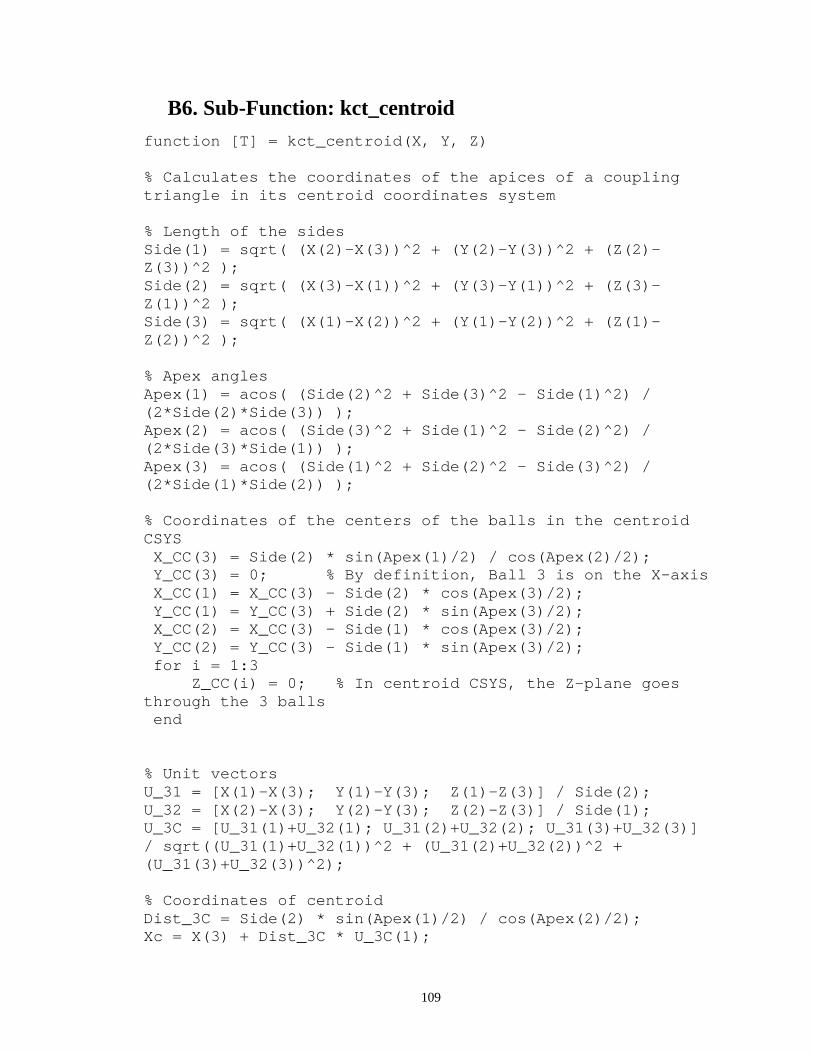
109

B6. Sub-Function: kct_centroid function [T] = kct_centroid(X, Y, Z) % Calculates the coordinates of the apices of a coupling triangle in its centroid coordinates system % Length of the sides Side(1) = sqrt( (X(2)-X(3))^2 + (Y(2)-Y(3))^2 + (Z(2)-Z(3))^2 ); Side(2) = sqrt( (X(3)-X(1))^2 + (Y(3)-Y(1))^2 + (Z(3)-Z(1))^2 ); Side(3) = sqrt( (X(1)-X(2))^2 + (Y(1)-Y(2))^2 + (Z(1)-Z(2))^2 ); % Apex angles Apex(1) = acos( (Side(2)^2 + Side(3)^2 - Side(1)^2) / (2*Side(2)*Side(3)) ); Apex(2) = acos( (Side(3)^2 + Side(1)^2 - Side(2)^2) / (2*Side(3)*Side(1)) ); Apex(3) = acos( (Side(1)^2 + Side(2)^2 - Side(3)^2) / (2*Side(1)*Side(2)) ); % Coordinates of the centers of the balls in the centroid CSYS X_CC(3) = Side(2) * sin(Apex(1)/2) / cos(Apex(2)/2); Y_CC(3) = 0; % By definition, Ball 3 is on the X-axis X_CC(1) = X_CC(3) - Side(2) * cos(Apex(3)/2); Y_CC(1) = Y_CC(3) + Side(2) * sin(Apex(3)/2); X_CC(2) = X_CC(3) - Side(1) * cos(Apex(3)/2); Y_CC(2) = Y_CC(3) - Side(1) * sin(Apex(3)/2); for i = 1:3 Z_CC(i) = 0; % In centroid CSYS, the Z-plane goes through the 3 balls end % Unit vectors U_31 = [X(1)-X(3); Y(1)-Y(3); Z(1)-Z(3)] / Side(2); U_32 = [X(2)-X(3); Y(2)-Y(3); Z(2)-Z(3)] / Side(1); U_3C = [U_31(1)+U_32(1); U_31(2)+U_32(2); U_31(3)+U_32(3)] / sqrt((U_31(1)+U_32(1))^2 + (U_31(2)+U_32(2))^2 + (U_31(3)+U_32(3))^2); % Coordinates of centroid Dist_3C = Side(2) * sin(Apex(1)/2) / cos(Apex(2)/2); Xc = X(3) + Dist_3C * U_3C(1);

110

Yc = Y(3) + Dist_3C * U_3C(2); Zc = Z(3) + Dist_3C * U_3C(3); Bc = asin((Zc-Z(3)) / X_CC(3)); % Rotation about the Y axis Ac = acos((X(3)-Xc) / (X_CC(3)*cos(Bc))); % Rotation about the Z axis Gc = asin((Z(2) - Zc + X_CC(2)*sin(Bc)) / (Y_CC(2)*cos(Bc))); % Rotation about the X axis % Set the elements within the homogenous transformation matrix T(1:4,1)=[cos(Ac)*cos(Bc); sin(Ac)*cos(Bc); -sin(Bc); 0]; T(1:4,2)=[cos(Ac)*sin(Bc)*sin(Gc)-sin(Ac)*cos(Gc); sin(Ac)*sin(Bc)*sin(Gc)+cos(Ac)*cos(Gc); cos(Bc)*sin(Gc); 0]; T(1:4,3)=[cos(Ac)*sin(Bc)*cos(Gc)+sin(Ac)*sin(Gc); sin(Ac)*sin(Bc)*cos(Gc)-cos(Ac)*sin(Gc); cos(Bc)*cos(Gc); 0]; T(1:4,4)=[Xc; Yc; Zc; 1];

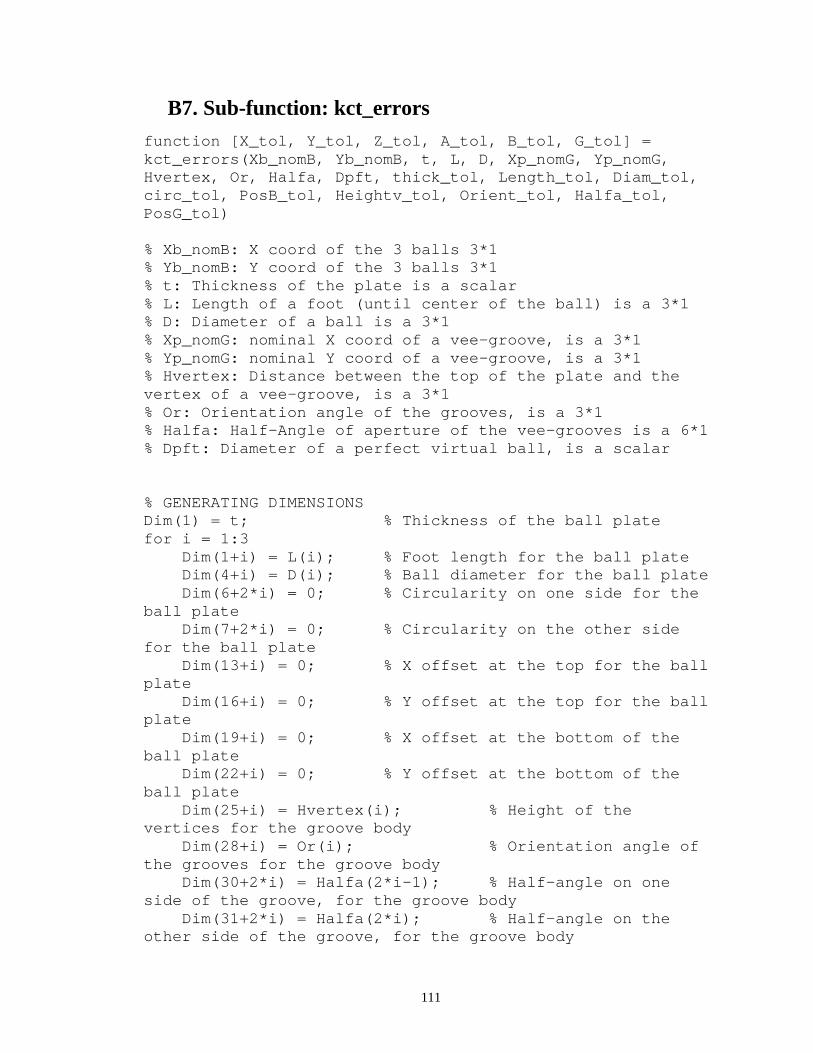
111

B7. Sub-function: kct_errors function [X_tol, Y_tol, Z_tol, A_tol, B_tol, G_tol] = kct_errors(Xb_nomB, Yb_nomB, t, L, D, Xp_nomG, Yp_nomG, Hvertex, Or, Halfa, Dpft, thick_tol, Length_tol, Diam_tol, circ_tol, PosB_tol, Heightv_tol, Orient_tol, Halfa_tol, PosG_tol) % Xb_nomB: X coord of the 3 balls 3*1 % Yb_nomB: Y coord of the 3 balls 3*1 % t: Thickness of the plate is a scalar % L: Length of a foot (until center of the ball) is a 3*1 % D: Diameter of a ball is a 3*1 % Xp_nomG: nominal X coord of a vee-groove, is a 3*1 % Yp_nomG: nominal Y coord of a vee-groove, is a 3*1 % Hvertex: Distance between the top of the plate and the vertex of a vee-groove, is a 3*1 % Or: Orientation angle of the grooves, is a 3*1 % Halfa: Half-Angle of aperture of the vee-grooves is a 6*1 % Dpft: Diameter of a perfect virtual ball, is a scalar % GENERATING DIMENSIONS Dim(1) = t; % Thickness of the ball plate for i = 1:3 Dim(1+i) = L(i); % Foot length for the ball plate Dim(4+i) = D(i); % Ball diameter for the ball plate Dim(6+2*i) = 0; % Circularity on one side for the ball plate Dim(7+2*i) = 0; % Circularity on the other side for the ball plate Dim(13+i) = 0; % X offset at the top for the ball plate Dim(16+i) = 0; % Y offset at the top for the ball plate Dim(19+i) = 0; % X offset at the bottom of the ball plate Dim(22+i) = 0; % Y offset at the bottom of the ball plate Dim(25+i) = Hvertex(i); % Height of the vertices for the groove body Dim(28+i) = Or(i); % Orientation angle of the grooves for the groove body Dim(30+2*i) = Halfa(2*i-1); % Half-angle on one side of the groove, for the groove body Dim(31+2*i) = Halfa(2*i); % Half-angle on the other side of the groove, for the groove body

112

Dim(37+i) = 0; % X offset of a pin, for the groove body Dim(40+i) = 0; % Y offset of a pin, for the groove body end N_dims = size(Dim,2); Varia(1) = thick_tol; % Thickness of the ball plate for i = 1:3 Varia(1+i) = Length_tol; % Foot length for the ball plate Varia(4+i) = Diam_tol; % Ball diameter for the ball plate Varia(6+2*i) = circ_tol; % Circularity on one side for the ball plate Varia(7+2*i) = circ_tol; % Circularity on the other side for the ball plate Varia(13+i) = PosB_tol; % X offset at the top for the ball plate Varia(16+i) = PosB_tol; % Y offset at the top for the ball plate Varia(19+i) = PosB_tol; % X offset at the bottom for the ball plate Varia(22+i) = PosB_tol; % Y offset at the bottom for the ball plate Varia(25+i) = Heightv_tol; % Height of the vertices for the groove body Varia(28+i) = Orient_tol; % Orientation angle of the grooves for the groove body Varia(30+2*i) = Halfa_tol; % Half-angle on one side of the groove, for the groove body Varia(31+2*i) = Halfa_tol; % Half-angle on the other side of the groove, for the groove body Varia(37+i) = PosG_tol; % X offset of a pin, for the groove body Varia(40+i) = PosG_tol; % Y offset of a pin, for the groove body end % CALCULATING THE JACOBIAN for i1 = 1:N_dims % the dimension we are looking at for i2 = 1: N_dims % loop to create the perturbed array if i1 == i2 Perturb(i2) = Dim(i2) + Varia(i2); else

113

Perturb(i2) = Dim(i2); end end t_p = Perturb(1); for i = 1:3 L_p(i) = Perturb(1+i); D_p(i) = Perturb(4+i); ci_B_p(2*i-1) = Perturb(6+2*i); ci_B_p(2*i) = Perturb(7+2*i); dXtop_B_p(i) = Perturb(13+i); dYtop_B_p(i) = Perturb(16+i); dXbot_B_p(i) = Perturb(19+i); dYbot_B_p(i) = Perturb(22+i); Hvertex_p(i) = Perturb(25+i); Or_p(i) = Perturb(28+i); Halfa_p(2*i-1) = Perturb(30+2*i); Halfa_p(2*i) = Perturb(31+2*i); dXpin_G_p(i) = Perturb(37+i); dYpin_G_p(i) = Perturb(40+i); end % For the ball pallet [X_B_BC, Y_B_BC, Z_B_BC, Db] = kct_ballgeom(Xb_nomB, Yb_nomB, t_p, L_p, D_p, ci_B_p, dXtop_B_p, dYtop_B_p, dXbot_B_p, dYbot_B_p); PB1=[X_B_BC(1); Y_B_BC(1); Z_B_BC(1); 1]; PB2=[X_B_BC(2); Y_B_BC(2); Z_B_BC(2); 1]; PB3=[X_B_BC(3); Y_B_BC(3); Z_B_BC(3); 1]; PB4=PB3; dB=Db'; % For the groove body [TG11_G, TG12_G, TG21_G, TG22_G, TG31_G, TG32_G] = kct_groovegeom(Xp_nomG, Yp_nomG, Hvertex_p, Or_p, Halfa_p, Dpft, dXpin_G_p, dYpin_G_p); % CALCULATING RESTING POSITION [alpha,beta,gamma,xr,yr,zr,Pc1,Pc2,Pc3,Pc4,Pc5,Pc6]=kct_rest(PB1,PB2,PB3,PB4,dB,TG11_G,TG12_G,TG21_G,TG22_G,TG31_G,TG32_G); dXdDim(i1) = xr / Varia(i1); dYdDim(i1) = yr / Varia(i1); dZdDim(i1) = zr / Varia(i1); dAdDim(i1) = alpha / Varia(i1); dBdDim(i1) = beta / Varia(i1); dGdDim(i1) = gamma / Varia(i1);

114

end Jacob = [dXdDim; dYdDim; dZdDim; dAdDim; dBdDim; dGdDim]; % COVARIANCE MATRICES CoMtx_Dim = zeros(N_dims,N_dims); for i = 1:N_dims CoMtx_Dim(i,i) = Varia(i)^2 / 9; end CoMtx_Err = Jacob * CoMtx_Dim * Jacob'; X_tol = 3 * sqrt(CoMtx_Err(1,1)); Y_tol = 3 * sqrt(CoMtx_Err(2,2)); Z_tol = 3 * sqrt(CoMtx_Err(3,3)); A_tol = 3 * sqrt(CoMtx_Err(4,4)); B_tol = 3 * sqrt(CoMtx_Err(5,5)); G_tol = 3 * sqrt(CoMtx_Err(6,6));

115

B8. Sub-Function: kct_groovegeom function [T_V11_GC, T_V12_GC, T_V21_GC, T_V22_GC, T_V31_GC, T_V32_GC] = kct_groovegeom(X_V_nomG, Y_V_nomG, Height_V_mfgG, Orient_mfgG, Halfangle, Diam, DeltaX_mfgG, DeltaY_mfgG) % X_V_nomG: nominal X coord of a vee-groove, is a 3*1 % Y_V_nomG: nominal Y coord of a vee-groove, is a 3*1 % Height_V_mfgG: Distance between the top of the plate and the vertex of a vee-groove, is a 3*1 % Orient_mfgG: Orientation angle of the grooves, is a 3*1 % Halfangle: Half-Angle of aperture of the vee-grooves is a 6*1 % Diam: Diameter of a perfect virtual ball, is a scalar % DeltaX_mfgG: X Offset of the pin, is a 3*1 % DeltaY_mfgG: Y Offset of the pin, is a 3*1 % FLAT SURFACES IN MFG COORDINATES SYSTEM % Translation of the vertex for ig = 1:3 X_V_mfgG(ig) = X_V_nomG(ig) + DeltaX_mfgG(ig); Y_V_mfgG(ig) = Y_V_nomG(ig) + DeltaY_mfgG(ig); end T_V_Tr_1 = [1 0 0 X_V_mfgG(1); 0 1 0 Y_V_mfgG(1); 0 0 1 Height_V_mfgG(1); 0 0 0 1]; T_V_Tr_2 = [1 0 0 X_V_mfgG(2); 0 1 0 Y_V_mfgG(2); 0 0 1 Height_V_mfgG(2); 0 0 0 1]; T_V_Tr_3 = [1 0 0 X_V_mfgG(3); 0 1 0 Y_V_mfgG(3); 0 0 1 Height_V_mfgG(3); 0 0 0 1]; % Rotation about the Z axis of the vertex T_V_RinZ_11 = [cos(Orient_mfgG(1)-pi/2) -sin(Orient_mfgG(1)-pi/2) 0 0; sin(Orient_mfgG(1)-pi/2) cos(Orient_mfgG(1)-pi/2) 0 0; 0 0 1 0; 0 0 0 1]; T_V_RinZ_12 = [cos(Orient_mfgG(1)+pi/2) -sin(Orient_mfgG(1)+pi/2) 0 0; sin(Orient_mfgG(1)+pi/2) cos(Orient_mfgG(1)+pi/2) 0 0; 0 0 1 0; 0 0 0 1]; T_V_RinZ_21 = [cos(Orient_mfgG(2)-pi/2) -sin(Orient_mfgG(2)-pi/2) 0 0; sin(Orient_mfgG(2)-pi/2) cos(Orient_mfgG(2)-pi/2) 0 0; 0 0 1 0; 0 0 0 1]; T_V_RinZ_22 = [cos(Orient_mfgG(2)+pi/2) -sin(Orient_mfgG(2)+pi/2) 0 0; sin(Orient_mfgG(2)+pi/2) cos(Orient_mfgG(2)+pi/2) 0 0; 0 0 1 0; 0 0 0 1];

116

T_V_RinZ_31 = [cos(Orient_mfgG(3)-pi/2) -sin(Orient_mfgG(3)-pi/2) 0 0; sin(Orient_mfgG(3)-pi/2) cos(Orient_mfgG(3)-pi/2) 0 0; 0 0 1 0; 0 0 0 1]; T_V_RinZ_32 = [cos(Orient_mfgG(3)+pi/2) -sin(Orient_mfgG(3)+pi/2) 0 0; sin(Orient_mfgG(3)+pi/2) cos(Orient_mfgG(3)+pi/2) 0 0; 0 0 1 0; 0 0 0 1]; % Rotation about the Y axis of the vertex T_V_RinY_11 = [cos(pi/2-Halfangle(1)) 0 sin(pi/2-Halfangle(1)) 0; 0 1 0 0; -sin(pi/2-Halfangle(1)) 0 cos(pi/2-Halfangle(1)) 0; 0 0 0 1]; T_V_RinY_12 = [cos(pi/2-Halfangle(2)) 0 sin(pi/2-Halfangle(2)) 0; 0 1 0 0; -sin(pi/2-Halfangle(2)) 0 cos(pi/2-Halfangle(2)) 0; 0 0 0 1]; T_V_RinY_21 = [cos(pi/2-Halfangle(3)) 0 sin(pi/2-Halfangle(3)) 0; 0 1 0 0; -sin(pi/2-Halfangle(3)) 0 cos(pi/2-Halfangle(3)) 0; 0 0 0 1]; T_V_RinY_22 = [cos(pi/2-Halfangle(4)) 0 sin(pi/2-Halfangle(4)) 0; 0 1 0 0; -sin(pi/2-Halfangle(4)) 0 cos(pi/2-Halfangle(4)) 0; 0 0 0 1]; T_V_RinY_31 = [cos(pi/2-Halfangle(5)) 0 sin(pi/2-Halfangle(5)) 0; 0 1 0 0; -sin(pi/2-Halfangle(5)) 0 cos(pi/2-Halfangle(5)) 0; 0 0 0 1]; T_V_RinY_32 = [cos(pi/2-Halfangle(6)) 0 sin(pi/2-Halfangle(6)) 0; 0 1 0 0; -sin(pi/2-Halfangle(6)) 0 cos(pi/2-Halfangle(6)) 0; 0 0 0 1]; % Combination of the transformations % You give coord in local CSYS, this matrix will return the coord in the mfg CSYS T_V11_mfgG = T_V_Tr_1 * T_V_RinZ_11 * T_V_RinY_11; T_V12_mfgG = T_V_Tr_1 * T_V_RinZ_12 * T_V_RinY_12; T_V21_mfgG = T_V_Tr_2 * T_V_RinZ_21 * T_V_RinY_21; T_V22_mfgG = T_V_Tr_2 * T_V_RinZ_22 * T_V_RinY_22; T_V31_mfgG = T_V_Tr_3 * T_V_RinZ_31 * T_V_RinY_31; T_V32_mfgG = T_V_Tr_3 * T_V_RinZ_32 * T_V_RinY_32; % GROOVE CENTROID IN MFG COORDINATES SYSTEM for ig = 1:3 Dist_CV(ig) = (Diam/2) / sin((Halfangle(2*ig-1) + Halfangle(2*ig)) / 2); % Distance between vertex and center of the ball X_G_mfgG(ig) = X_V_mfgG(ig) - Dist_CV(ig) * sin((Halfangle(2*ig-1) - Halfangle(2*ig)) /2) * sin(Orient_mfgG(ig));

117

Y_G_mfgG(ig) = Y_V_mfgG(ig) + Dist_CV(ig) * sin((Halfangle(2*ig-1) - Halfangle(2*ig)) /2) * cos(Orient_mfgG(ig)); Z_G_mfgG(ig) = Height_V_mfgG(ig) + Dist_CV(ig) * cos((Halfangle(2*ig-1) - Halfangle(2*ig)) /2); end T_GC_mfgG = kct_centroid(X_G_mfgG, Y_G_mfgG, Z_G_mfgG); % You give coord in centroid CSYS, this matrix will return the coord in the mfg CSYS % FLAT SURFACES IN GROOVE CENTROID COORDINATES SYSTEM T_V11_GC = inv(T_GC_mfgG) * T_V11_mfgG; T_V12_GC = inv(T_GC_mfgG) * T_V12_mfgG; T_V21_GC = inv(T_GC_mfgG) * T_V21_mfgG; T_V22_GC = inv(T_GC_mfgG) * T_V22_mfgG; T_V31_GC = inv(T_GC_mfgG) * T_V31_mfgG; T_V32_GC = inv(T_GC_mfgG) * T_V32_mfgG;

118

B9. Sub-Function: kct_perturb close all; clear all; % Perturbations % INPUT % For the ball pallet Xb_nomB = [1 1 7] * 25.4; % Fixed Yb_nomB = [7 1 4] * 25.4; % Fixed t = 6.35; L = [0.75 0.75 0.75] * 25.4; D = [0.5 0.5 0.5] * 25.4; % For the groove body Xp_nomG = [1.0 1.0 7.0] * 25.4; % Fixed Yp_nomG = [7.0 1.0 4.0] * 25.4; % Fixed Hvertex = [0.1 0.1 0.1] * 25.4; Or = [-60 60 180] * pi/180; Halfa = [45 45 45 45 45 45] * pi/180; Dpft = 12.7; % Fixed % TOLERANCES thick_tol = 0.02; Length_tol = 0.05; Diam_tol = 0.03; circ_tol = 0.01; XB_tol = 0.05; YB_tol = 0.05; Heightv_tol = 0.05; Orient_tol = 0.002; Halfa_tol = 0.003; XG_tol = 0.05; YG_tol = 0.05; % GENERATING DIMENSIONS Dim(1) = t; % Thickness of the ball plate for i = 1:3 Dim(1+i) = L(i); % Foot length for the ball plate Dim(4+i) = D(i); % Ball diameter for the ball plate Dim(6+2*i) = 0; % Circularity on one side for the ball plate Dim(7+2*i) = 0; % Circularity on the other side for the ball plate

119

Dim(13+i) = 0; % X offset at the top for the ball plate Dim(16+i) = 0; % Y offset at the top for the ball plate Dim(19+i) = 0; % X offset at the bottom of the ball plate Dim(22+i) = 0; % Y offset at the bottom of the ball plate Dim(25+i) = Hvertex(i); % Height of the vertices for the groove body Dim(28+i) = Or(i); % Orientation angle of the grooves for the groove body Dim(30+2*i) = Halfa(2*i-1); % Half-angle on one side of the groove, for the groove body Dim(31+2*i) = Halfa(2*i); % Half-angle on the other side of the groove, for the groove body Dim(37+i) = 0; % X offset of a pin, for the groove body Dim(40+i) = 0; % Y offset of a pin, for the groove body end N_dims = size(Dim,2); Varia(1) = thick_tol; % Thickness of the ball plate for i = 1:3 Varia(1+i) = Length_tol; % Foot length for the ball plate Varia(4+i) = Diam_tol; % Ball diameter for the ball plate Varia(6+2*i) = circ_tol; % Circularity on one side for the ball plate Varia(7+2*i) = circ_tol; % Circularity on the other side for the ball plate Varia(13+i) = XB_tol; % X offset at the top for the ball plate Varia(16+i) = YB_tol; % Y offset at the top for the ball plate Varia(19+i) = XB_tol; % X offset at the bottom for the ball plate Varia(22+i) = YB_tol; % Y offset at the bottom for the ball plate Varia(25+i) = Heightv_tol; % Height of the vertices for the groove body Varia(28+i) = Orient_tol; % Orientation angle of the grooves for the groove body Varia(30+2*i) = Halfa_tol; % Half-angle on one side of the groove, for the groove body

120

Varia(31+2*i) = Halfa_tol; % Half-angle on the other side of the groove, for the groove body Varia(37+i) = XG_tol; % X offset of a pin, for the groove body Varia(40+i) = YG_tol; % X offset of a pin, for the groove body end % CALCULATING THE JACOBIAN for i1 = 1:N_dims % the dimension we are looking at for i2 = 1: N_dims % loop to create the perturbed array if i1 == i2 Perturb(i2) = Dim(i2) + Varia(i2); else Perturb(i2) = Dim(i2); end end t_p = Perturb(1); for i = 1:3 L_p(i) = Perturb(1+i); D_p(i) = Perturb(4+i); ci_B_p(2*i-1) = Perturb(6+2*i); ci_B_p(2*i) = Perturb(7+2*i); dXtop_B_p(i) = Perturb(13+i); dYtop_B_p(i) = Perturb(16+i); dXbot_B_p(i) = Perturb(19+i); dYbot_B_p(i) = Perturb(22+i); Hvertex_p(i) = Perturb(25+i); Or_p(i) = Perturb(28+i); Halfa_p(2*i-1) = Perturb(30+2*i); Halfa_p(2*i) = Perturb(31+2*i); dXpin_G_p(i) = Perturb(37+i); dYpin_G_p(i) = Perturb(40+i); end % For the ball pallet [X_B_BC, Y_B_BC, Z_B_BC, Db] = kct_ballgeom(Xb_nomB, Yb_nomB, t_p, L_p, D_p, ci_B_p, dXtop_B_p, dYtop_B_p, dXbot_B_p, dYbot_B_p); PB1=[X_B_BC(1); Y_B_BC(1); Z_B_BC(1); 1]; PB2=[X_B_BC(2); Y_B_BC(2); Z_B_BC(2); 1]; PB3=[X_B_BC(3); Y_B_BC(3); Z_B_BC(3); 1]; PB4=PB3; dB=Db';

121

% For the groove body [TG11_G, TG12_G, TG21_G, TG22_G, TG31_G, TG32_G] = kct_groovegeom(Xp_nomG, Yp_nomG, Hvertex_p, Or_p, Halfa_p, Dpft, dXpin_G_p, dYpin_G_p); % CALCULATING RESTING POSITION [alpha,beta,gamma,xr,yr,zr,Pc1,Pc2,Pc3,Pc4,Pc5,Pc6]=kct_rest(PB1,PB2,PB3,PB4,dB,TG11_G,TG12_G,TG21_G,TG22_G,TG31_G,TG32_G); dXdDim(i1) = xr / Varia(i1); dYdDim(i1) = yr / Varia(i1); dZdDim(i1) = zr / Varia(i1); dAdDim(i1) = alpha / Varia(i1); dBdDim(i1) = beta / Varia(i1); dGdDim(i1) = gamma / Varia(i1); end Jacob = [dXdDim; dYdDim; dZdDim; dAdDim; dBdDim; dGdDim] % COVARIANCE MATRICES CoMtx_Dim = zeros(N_dims,N_dims); for i = 1:N_dims CoMtx_Dim(i,i) = Varia(i)^2 / 9; end CoMtx_Err = Jacob * CoMtx_Dim * Jacob' X_tol = 3 * sqrt(CoMtx_Err(1,1)) Y_tol = 3 * sqrt(CoMtx_Err(2,2)) Z_tol = 3 * sqrt(CoMtx_Err(3,3)) A_tol = 3 * sqrt(CoMtx_Err(4,4)) B_tol = 3 * sqrt(CoMtx_Err(5,5)) G_tol = 3 * sqrt(CoMtx_Err(6,6))

122

B10. Sub-Function: kct_rest function [alpha,beta,gamma,xr,yr,zr,Pc1,Pc2,Pc3,Pc4,Pc5,Pc6]=kct_rest(PB1,PB2,PB3,PB4,dB,TG11_G,TG12_G,TG21_G,TG22_G,TG31_G,TG32_G) % This function calls the fsolve routine to solve the 24 nonlinear equations that provide the resting position of the ball body of a kinematic coupling in a groove body. Vectors PB1, PB2, PB3, and PB4 locate the centers of the balls in coordinate sytem located at the coupling centroid. TG11_G,TG12_G,TG21_G,TG22_G,TG31_G, and TG32_G are the transformations from groove surfaces to groove coordinate system (ideally equal to ball coupling centroid). alpha, beta, and gamma, are rotations about x,y, and z, respectively. xr, yr, and zr are displacements, and Pc1,Pc2,Pc3,Pc4,Pc5, and Pc6 are position vectors to the contact points. % Setup initial guesses for unknowns for i=1:6 vars(i)=0; % Initial guess for the error components are all set to zero end vars(7:9)=PB1(1:3); % Initial guess for the coordinates of contact point #1 are set to the center of ball #1 vars(10:12)=PB1(1:3); % Initial guess for the coordinates of contact point #2 are set to the center of ball #2 vars(13:15)=PB2(1:3); % Initial guess for the coordinates of contact point #3 are set to the center of ball #3 vars(16:18)=PB2(1:3); % Initial guess for the coordinates of contact point #4 are set to the center of ball #4 vars(19:21)=PB3(1:3); % Initial guess for the coordinates of contact point #5 are set to the center of ball #5 vars(22:24)=PB3(1:3); % Initial guess for the coordinates of contact point #6 are set to the center of ball #6 vars=vars'; % Setup params vector to pass variables to fsolve routine params(1:3)=PB1(1:3); params(4:6)=PB2(1:3); params(7:9)=PB3(1:3); params(10:12)=PB4(1:3); params(13:15)=TG11_G(1:3,1); params(16:18)=TG11_G(1:3,2); params(19:21)=TG11_G(1:3,3); params(22:24)=TG11_G(1:3,4);

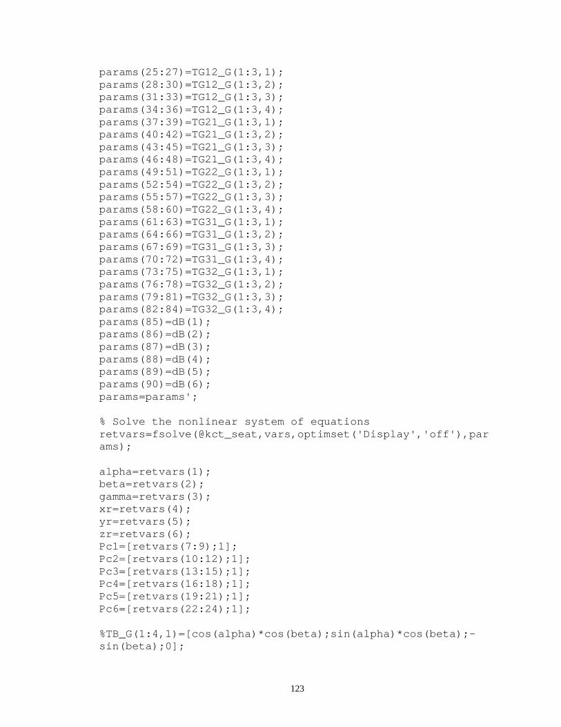
123

params(25:27)=TG12_G(1:3,1); params(28:30)=TG12_G(1:3,2); params(31:33)=TG12_G(1:3,3); params(34:36)=TG12_G(1:3,4); params(37:39)=TG21_G(1:3,1); params(40:42)=TG21_G(1:3,2); params(43:45)=TG21_G(1:3,3); params(46:48)=TG21_G(1:3,4); params(49:51)=TG22_G(1:3,1); params(52:54)=TG22_G(1:3,2); params(55:57)=TG22_G(1:3,3); params(58:60)=TG22_G(1:3,4); params(61:63)=TG31_G(1:3,1); params(64:66)=TG31_G(1:3,2); params(67:69)=TG31_G(1:3,3); params(70:72)=TG31_G(1:3,4); params(73:75)=TG32_G(1:3,1); params(76:78)=TG32_G(1:3,2); params(79:81)=TG32_G(1:3,3); params(82:84)=TG32_G(1:3,4); params(85)=dB(1); params(86)=dB(2); params(87)=dB(3); params(88)=dB(4); params(89)=dB(5); params(90)=dB(6); params=params'; % Solve the nonlinear system of equations retvars=fsolve(@kct_seat,vars,optimset('Display','off'),params); alpha=retvars(1); beta=retvars(2); gamma=retvars(3); xr=retvars(4); yr=retvars(5); zr=retvars(6); Pc1=[retvars(7:9);1]; Pc2=[retvars(10:12);1]; Pc3=[retvars(13:15);1]; Pc4=[retvars(16:18);1]; Pc5=[retvars(19:21);1]; Pc6=[retvars(22:24);1]; %TB_G(1:4,1)=[cos(alpha)*cos(beta);sin(alpha)*cos(beta);-sin(beta);0];

124

%TB_G(1:4,2)=[cos(alpha)*sin(beta)*sin(gamma)-sin(alpha)*cos(gamma);sin(alpha)*sin(beta)*sin(gamma)+cos(alpha)*cos(gamma);cos(beta)*sin(gamma);0]; %TB_G(1:4,3)=[cos(alpha)*sin(beta)*cos(gamma)+sin(alpha)*sin(gamma);sin(alpha)*sin(beta)*cos(gamma)-cos(alpha)*sin(gamma);cos(beta)*cos(gamma);0]; %TB_G(1:4,4)=[xr;yr;zr;1];

125

B11. Sub-Function: kct_seat function retvars=kct_seat(vars, params) % This function evaluates the 24 functions that are the system of non-linear equations that can be solved for the seating position (transformation) of the ball body in the groove body. When used with fsolve.m the system can be solved for the x,y,z,alpha,beta, and gamma pose coordinates as well as the coordinates of the 6 contact points. This function must be sent the positions of the balls in a coordinate system located at the coupling centroid, the contact normal vectors, and the ball diameter in the components of the vector params. alpha=vars(1); % Rotation angle about z-axis beta=vars(2); % Rotation angle about y-axis gamma=vars(3); % Rotation angle about x-axis xr=vars(4); % Position in x-axis yr=vars(5); % Position in y-axis zr=vars(6); % Position in z-axis Pc1(1:4)=[vars(7:9);1]; Pc1=Pc1'; % Contact point 1's coordinates Pc2(1:4)=[vars(10:12);1]; Pc2=Pc2'; % Contact point 2's coordinates Pc3(1:4)=[vars(13:15);1]; Pc3=Pc3'; % Contact point 3's coordinates Pc4(1:4)=[vars(16:18);1]; Pc4=Pc4'; % Contact point 4's coordinates Pc5(1:4)=[vars(19:21);1]; Pc5=Pc5'; % Contact point 5's coordinates Pc6(1:4)=[vars(22:24);1]; Pc6=Pc6'; % Contact point 6's coordinates % Extract values in params vector into meaningful notation Pb1=[params(1:3)];Pb1(4)=1; % Position of ball 1 in coordinate system at coupling centroid in ball body Pb2=[params(4:6)];Pb2(4)=1; % Position of ball 2 in coordinate system at coupling centroid in ball body Pb3=[params(7:9)];Pb3(4)=1; % Position of ball 3 in coordinate system at coupling centroid in ball body Pb4=[params(10:12)];Pb4(4)=1; % Position of ball 4 in coordinate system at coupling centroid in ball body TG11_G=[params(13:15),params(16:18),params(19:21),params(22:24)]; % Transformation from surface 1_1 to Groove coord system TG11_G(4,1:4)=[0,0,0,1];

126

TG12_G=[params(25:27),params(28:30),params(31:33),params(34:36)]; % Transformation from surface 1_2 to Groove coord system TG12_G(4,1:4)=[0,0,0,1]; TG21_G=[params(37:39),params(40:42),params(43:45),params(46:48)]; % Transformation from surface 2_1 to Groove coord system TG21_G(4,1:4)=[0,0,0,1]; TG22_G=[params(49:51),params(52:54),params(55:57),params(58:60)]; % Transformation from surface 2_2 to Groove coord system TG22_G(4,1:4)=[0,0,0,1]; TG31_G=[params(61:63),params(64:66),params(67:69),params(70:72)]; % Transformation from surface 3_1 to Groove coord system TG31_G(4,1:4)=[0,0,0,1]; TG32_G=[params(73:75),params(76:78),params(79:81),params(82:84)]; % Transformation from surface 3_2 to Groove coord system TG32_G(4,1:4)=[0,0,0,1]; rB(1)=params(85)/2; % Radius of Balls rB(2)=params(86)/2; rB(3)=params(87)/2; rB(4)=params(88)/2; rB(5)=params(89)/2; rB(6)=params(90)/2; %Extract normal vectors at contact points from the transformation matrices n1=[TG11_G(1:3,3);1]; % Unit vector in direction of contact force 1 at contact point 1 n2=[TG12_G(1:3,3);1]; % Unit vector in direction of contact force 2 at contact point 2 n3=[TG21_G(1:3,3);1]; % Unit vector in direction of contact force 3 at contact point 3 n4=[TG22_G(1:3,3);1]; % Unit vector in direction of contact force 4 at contact point 4 n5=[TG31_G(1:3,3);1]; % Unit vector in direction of contact force 5 at contact point 5 n6=[TG32_G(1:3,3);1]; % Unit vector in direction of contact force 6 at contact point 6 % Calculate elements within the homogenous transformation matrix representing resting position T(1:4,1)=[cos(alpha)*cos(beta);sin(alpha)*cos(beta);-sin(beta);0];

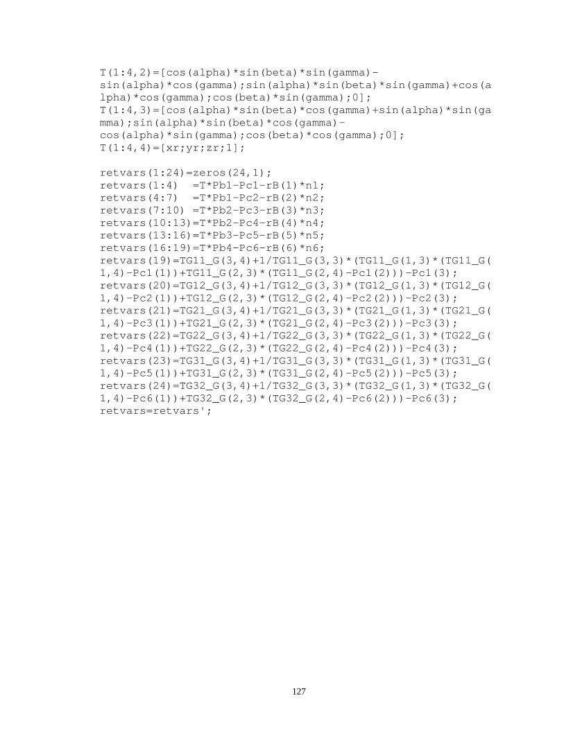
127

T(1:4,2)=[cos(alpha)*sin(beta)*sin(gamma)-sin(alpha)*cos(gamma);sin(alpha)*sin(beta)*sin(gamma)+cos(alpha)*cos(gamma);cos(beta)*sin(gamma);0]; T(1:4,3)=[cos(alpha)*sin(beta)*cos(gamma)+sin(alpha)*sin(gamma);sin(alpha)*sin(beta)*cos(gamma)-cos(alpha)*sin(gamma);cos(beta)*cos(gamma);0]; T(1:4,4)=[xr;yr;zr;1]; retvars(1:24)=zeros(24,1); retvars(1:4) =T*Pb1-Pc1-rB(1)*n1; retvars(4:7) =T*Pb1-Pc2-rB(2)*n2; retvars(7:10) =T*Pb2-Pc3-rB(3)*n3; retvars(10:13)=T*Pb2-Pc4-rB(4)*n4; retvars(13:16)=T*Pb3-Pc5-rB(5)*n5; retvars(16:19)=T*Pb4-Pc6-rB(6)*n6; retvars(19)=TG11_G(3,4)+1/TG11_G(3,3)*(TG11_G(1,3)*(TG11_G(1,4)-Pc1(1))+TG11_G(2,3)*(TG11_G(2,4)-Pc1(2)))-Pc1(3); retvars(20)=TG12_G(3,4)+1/TG12_G(3,3)*(TG12_G(1,3)*(TG12_G(1,4)-Pc2(1))+TG12_G(2,3)*(TG12_G(2,4)-Pc2(2)))-Pc2(3); retvars(21)=TG21_G(3,4)+1/TG21_G(3,3)*(TG21_G(1,3)*(TG21_G(1,4)-Pc3(1))+TG21_G(2,3)*(TG21_G(2,4)-Pc3(2)))-Pc3(3); retvars(22)=TG22_G(3,4)+1/TG22_G(3,3)*(TG22_G(1,3)*(TG22_G(1,4)-Pc4(1))+TG22_G(2,3)*(TG22_G(2,4)-Pc4(2)))-Pc4(3); retvars(23)=TG31_G(3,4)+1/TG31_G(3,3)*(TG31_G(1,3)*(TG31_G(1,4)-Pc5(1))+TG31_G(2,3)*(TG31_G(2,4)-Pc5(2)))-Pc5(3); retvars(24)=TG32_G(3,4)+1/TG32_G(3,3)*(TG32_G(1,3)*(TG32_G(1,4)-Pc6(1))+TG32_G(2,3)*(TG32_G(2,4)-Pc6(2)))-Pc6(3); retvars=retvars';

128

Appendix C:

Determining the HTM from a Metrology Datum Frame to a Centroidal Coordinate System

The coordinates of the triangles’ three apices B1 ( )111

,, BD

BD

BD zyx , B2

( )222

,, BD

BD

BD zyx and B3 ( )

333,, B

DB

DB

D zyx are measured in a metrology datum frame,

denoted with the prescript D, as shown in Fig C1.

x

y

z

C

B1

B3B2

x

z

y

DAngle

BisectorsDatum

Coordinates

CentroidCoordinates

Fig C1: Datum and Centroid Coordinate Systems in Coupling Triangle

The centroidal coordinate system, denoted with the prescript C, is defined by

three criteria:

� Its origin is located at the intersection of the triangle’s bisectors, which is the centroid

C.

� Its x-axis points towards B3.

� The three apices B1, B2 and B3 lie in the xy-plane.

Criterion � implies that the z-coordinates of the apices are equal to zero, as

shown in Eq (C1):

0321

=== BC

BC

BC zzz (C1)

129

The complete geometry of triangle (B1B2B3) is determined by calculating the edge

lengths using Eq (C2)-(C4) and the internal angles using Eq (C5)-(C7).

( ) ( ) ( )

( ) ( ) ( )

( ) ( ) ( )222

13

222

32

222

21

313131

232323

121212

BD

BD

BD

BD

BD

BD

BD

BD

BD

BD

BD

BD

BD

BD

BD

BD

BD

BD

zzyyxxBB

zzyyxxBB

zzyyxxBB

−+−+−=

−+−+−=

−+−+−=

(C2)

(C3)

(C4)

××

−+=∠

××

−+=∠

××

−+=∠

1332

221

213

232

3

3221

213

232

221

2

2113

232

221

213

1

2arccos

2arccos

2arccos

BBBB

BBBBBBB

BBBB

BBBBBBB

BBBB

BBBBBBB

(C5)

(C6)

(C7)

Applying the law of sine’s in triangle (B1CB3) gives Eq (C8):

( )31

13

1

3

sin2

sinCBB

BBB

CB

∠=

∠

(C8)

Since the three angles of a triangle are supplementary, triangle (B1CB3) provides

Eq (C9).

133131 BCBBCBCBB ∠−∠−=∠ π (C9)

Applying the same rule on triangle (B1B2B3) gives Eq (C10):

312 BBB ∠−∠−=∠ π (C10)

By definition, the bisectors divide the triangle’s internal angles into two equal

angles. This rule gives Eq (C11) and Eq (C12).

21

31

BBCB

∠=∠ (C11)

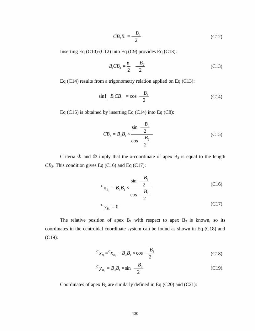
130

23

13

BBCB

∠=∠ (C12)

Inserting Eq (C10)-(C12) into Eq (C9) provides Eq (C13):

222

31

BCBB

∠+=∠ π

(C13)

Eq (C14) results from a trigonometry relation applied on Eq (C13):

( )

∠=∠

2cossin 2

31

BCBB (C14)

Eq (C15) is obtained by inserting Eq (C14) into Eq (C8):

∠

∠

×=⇒

2cos

2sin

2

1

133 B

B

BBCB (C15)

Criteria � and � imply that the x-coordinate of apex B3 is equal to the length

CB3. This condition gives Eq (C16) and Eq (C17):

=

∠

∠

×=

0

2cos

2sin

3

32

1

13

BC

BC

y

B

B

BBx

(C16)

(C17)

The relative position of apex B1 with respect to apex B3 is known, so its

coordinates in the centroidal coordinate system can be found as shown in Eq (C18) and

(C19):

∠

×=

∠

×−=

2sin

2cos

313

313

1

31

BBBy

BBBxx

BC

BC

BC

(C18)

(C19)

Coordinates of apex B2 are similarly defined in Eq (C20) and (C21):

131

∠

×=

∠

×−=

2sin

2cos

321

321

1

32

BBBy

BBBxx

BC

BC

BC

(C20)

(C21)

Finding the rotation angles about the three axes of the centroidal coordinate

system requires the definition of three distinct unit vectors that start from apex B3 and

point respectively towards B1, B2 and C. The coordinates of these unit vectors in the

metrology datum frame are presented in Eq (C22)-(C24):

−

−

−

×=

31

31

31

13

13

1

BD

BD

BD

BD

BD

BD

BBD

zz

yy

xx

BBur

−

−

−

×=

32

32

32

23

32

1

BD

BD

BD

BD

BD

BD

BBD

zz

yy

xx

BBur

( ) ( ) ( )

+

+

+

×+++++

=

zBB

DzBB

D

yBB

DyBB

D

xBB

DxBB

D

zBB

DzBB

DyBB

DyBB

DxBB

DxBB

DCB

D

uu

uu

uu

uuuuuuu

2313

2313

2313

231323132313

3 222

1r

(C22)

(C23)

(C24)

Then the coordinates of the centroid C in the metrology datum frame are defined

by Eq (C25)-(C27):

×+=

×+=

×+=

zCB

DB

DC

D

yCB

DB

DC

D

xCB

DB

DC

D

uCBzz

uCByy

uCBxx

33

33

33

3

3

3

(C25)

(C26)

(C27)

Hence the rotation βCD about the y-axis, between the two coordinate systems, is

obtained by Eq (C28):

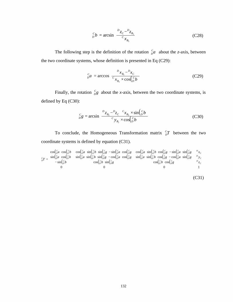
132

−=

3

3arcsinB

C

BD

CD

CD x

zzβ (C28)

The following step is the definition of the rotation αCD about the z-axis, between

the two coordinate systems, whose definition is presented in Eq (C29):

( )

×

−=

βα

CDB

C

CD

BD

CD x

xx

cosarccos

3

3 (C29)

Finally, the rotation γCD about the x-axis, between the two coordinate systems, is

defined by Eq (C30):

( )( )

×

×+−=

β

βγ

CDB

C

CDB

CC

DB

DCD y

xzz

cos

sinarcsin

2

22 (C30)

To conclude, the Homogeneous Transformation matrix TCD between the two

coordinate systems is defined by equation (C31).

( ) ( ) ( ) ( ) ( ) ( ) ( ) ( ) ( ) ( ) ( ) ( )( ) ( ) ( ) ( ) ( ) ( ) ( ) ( ) ( ) ( ) ( ) ( )

( ) ( ) ( ) ( ) ( )

−−−−−

=

1000

coscossincossin

sincoscossinsincoscossinsinsincossin

sinsincossincoscossinsinsincoscoscos

CDC

DCD

CD

CD

CD

CDC

DCD

CD

CD

CD

CD

CD

CD

CD

CD

CD

CD

CDC

DCD

CD

CD

CD

CD

CD

CD

CD

CD

CD

CD

CD

z

y

x

Tγβγββ

γαγβαγαγβαβαγαγβαγαγβαβα

(C31)

133

References [1] Slocum AH. Precision Machine Design, SME Press. Dearborn, Michigan. 1992.

[2] Slocum AH. “Kinematic Couplings for Precision Fixturing – Part I: Formulation of

Design Parameters”. Precision Engineering. Vol. 10, No. 2. 1988. P. 85-91.

[3] Schmiechen P. & Slocum AH. “Analysis of Kinematic Systems: a Generalized

Approach”. Precision Engineering. Vol. 19, no.1. 1996. P. 11-18.

[4] Vallance RR. & Slocum AH. “Kinematic Couplings for Pallets in Flexible

Assembly Systems”. Proceedings of the 15th Annual Meeting of the ASPE. Scottsdale,

AZ. October 22-27, 2000.

[5] Blanding DL. Exact Constraint: Machine Design Using Kinematic Principles. SME

Press. New York. 1999.

[6] International Organization for Standardization, ISO 3952-1: Kinematic Diagram –

Graphical Symbols. Geneva, Switzerland. 1981.

[7] American National Standards Institute, ASME/ANSI Y14.5M: Dimensioning and

Tolerancing. New York. 1994.

[8] International Organization for Standardization, ISO 129: Technical Drawings –

Dimensioning – General Principles, Definitions, Methods of Execution and Special

Indications. Geneva, Switzerland. 1985

[9] Groover MP. Automation, Production Systems, and Computer-Integrated

Manufacturing. Prentice-Hall. Upper Saddle River, New Jersey. 2001.

[10] Chase KW. “Tolerance Allocation Methods for Designers”, ADCATS Report No.

99-6. Brigham Young University, Utah. 1999.

[11] Hansen BL. Quality Control: Theory and Applications. Prentice-Hall. Upper Saddle

River, New Jersey. 1963.

[12] Venkataraman P. Applied Optimization with MATLAB® Programming. John Wiley

& sons, New York. 2002.

134

[13] Déplanche Y. Mémo Formulaire. Editions Casteilla. Paris, France. 1991.

[14] Craig JJ. Introduction to Robotics. Addison-Wesley Publishing Company. Palo Alto,

California. 1989.

[15] Clifford AA. Multivariate Error Analysis. John Wiley & Sons. New York. 1973.

[16] Serrano SE. Engineering Uncertainty and Risk Analysis. HydroScience Inc.

Lexington, Kentucky. 2001.

[17] Rubinstein RY. Simulation and the Monte Carlo Method. John Wiley & Sons. New

York. 1981.

[18] Hii KF. Kinematically Constrained Spindles. MSME Thesis. University of

Kentucky, Lexington, KY. 2002.

[19] Chase KW & Greenwood WH. “Design Issues in Mechanical Tolerance Analysis”.

Manufacturing Review. Vol.1, No 1. March 1988. pp 50-59.

[20] Doty LA. Statistical Process Control. Indutrial Press Inc. New York, 1996.

[21] Samson C, Hart P & Rubin C. Fundamentals of Statistical Quality Control.

Addison-Wesley Publishing Company. Reading, MA, 1970.

[22] Barlier C & Poulet B. Mémotech Génie Mécanique. Editions Casteilla. Paris, France,

1993.

[23] Conversation with KW Chase at the ASPE Summer Topical Meeting on Tolerance

Modeling and Analysis. Charlotte, NC. July 15-16, 2002.

[24] Chase KC, Gao J, Magleby SP & Sorensen CD. “Including Geometric Feature

Variations in Tolerance Analysis of Mechanical Assemblies”. IIE Transactions. Vol. 28,

1996. pp 795-807.

[25] Arenberg JW. “On the Origins of the Law of Error Propagation and its Uses”.

Proceedings of the ASPE 2002 Summer Topical Meeting, Charlotte, NC, pp 80-84.

[26] Vallance RR. Precision Connector Assembly Automation. PhD Thesis.

Massachusetts Institute of Technology. Cambridge, MA, USA. 1999.

135

[27] Ray WH & Szekely J. Process Optimization with Applications in Metallurgy and

Chemical Engineering. John Wiley & Sons, Inc. New York, 1973.

[28] Zanger H & Zanger C. Fiber Optics, Communication and Other Applications.

Macmillan Publishing Company, New York, 1991.

[29] Marcuse D. “Loss Analysis of Single-Mode Fiber Splices”. The Bell System

Technical Journal. May-June 1977. pp. 703-718.

[30] Gangopadhyay S & Sarkar SN. “Misalignment Considerations in Laser Diode to

Single-Mode Fiber Excitation via Hemispherical Lens on the Fiber Tip”. Journal of

Optical Communications. Vol. 19, No 6. Dec 1998.

[31] Jebens R, Trimmer W & Walker J. “Microactuators for aligning optical fibers”.

Sensors and Actuators. Vol. 20, No 1-2. Nov 1989. pp 65-73.

[32] Haibara T, Nakashima T, Matsumoto M & Hanafusa H. “Connection loss reduction

by thermally-diffused expanded core fiber”. IEEE Photonics Technology Letters. Vol. 3,

No 4. Apr 1991. pp 348-350.

[33] Cook S. “Composite Ferrules Pass Optical-Fiber Connector Performance Tests”.

Lightwave. Vol. 16, No 5. Apr 1999. pp 85-86.

[34] Iizuka Y et al. “Injection Molded Multifiber Optical Connector Using Thermoplastic

Resin”. Fujikura Technical Review. 2001. pp 17-23.

[35] Dunkel K et al. “Injection-moulded fibre ribbon connectors for parallel optical links

fabricated by the LIGA technique”. Journal of Micromechanics and Microengineering.

Vol. 8. 1998. pp 301-306.

[36] Poteat TL. “Submicron Accuracies in Anisotropic Etched Silicon Piece Parts – A

Case Study”. Studies in Electrical and Electronic Engineering Micromachining and

Micropackaging of Transducers. Vol. 20. 1985.

[37] Ohta T, Sigematsu T, Kihara Y & Kawazoe H. “Low loss single-mode multi-fiber

plastic connector”. Proceedings of International Wire and Cable Symposium Proceedings

of 38th International Wire and Cable Symposium (IWCS). Nov 14-16 1989. Atlanta, GA.

136

[38] Concejo T & Takeuchi H. “A New Glass-Ceramic Ferrule Technology for Optical

Connectors”. Lightwave. Vol. 16, No. 12. 1999. pp 86-87.

[39] Broadwater K & Mead PF. “Experimental and Numerical Studies in the Evaluation

of Epoxy-Cured Fiber Optic Connectors”. Proceedings of the 2000 Electronic

Components and Technology Conference. 2000. pp 981-988.

[40] Breedis JB. “Monte Carlo Tolerance Analysis of a Passively Aligned Silicon

Waferboard Package”. Proceedings of the 2001 Electronic Component and Technology

Conference. 2001.

[41] Uhing J, Thomas S & Christodoulou C. “A Statistical Approach for Estimating the

Loss Contribution of Concatenated Connectors in Fiber-Optic Links”. Proceedings of the

1990 Electronic Component and Technology Conference. 1990. pp 239-245.

[42] Rachakonda P, Barraja M, Vallance RR, Kiani S & Lehman J. “2D Error Models

and Monte Carlo Simulations for Budgeting Variation in Optical-Fiber Array

Connectors”. Proceedings of the ASPE 2001 Annual Meeting. pp 509-512.

[43] Madou M. Fundamentals of Microfabrication. CRC Press. New York. 1997.

[44] Vasile MJ, Friedrich CR, Kikkeri B & McElhannon R. "Micrometer-Scale

Machining: Tool Fabrication and Initial Results". Precision Engineering. Vol. 19.

1996. p. 180-186.

[45] Schaller Th, Bohn L, Mayer J & Schubert K. “Microstructure Grooves with a Width

of Less than 50 µm cut with Ground Hard Metal Micro End Mills”. Precision

Engineering. Vol. 23, No. 4. October 1999. p. 229-235.

[46] Masuzawa T & Tönshoff HK. "Three-Dimensional Micromachining by Machine

Tools". Keynote Paper. Annals of the CIRP. Vol. 46, No. 2. 1997. p. 621-628.

[47] Hirt G & Rattay B. “Coining of Thin Plates to Produce Micro Channel Structures”.

Initiatives of Precision Engineering at the Beginning of a Millennium. Proceedings of the

10th Int. Conf. on Precision Engineering. JSPE. Yokohama, Japan. July 18-20, 2001.

Kluwer Academic Publishers, Boston, MA. p. 32-36.

137

[48] Lee K, Stirn B & Dornfeld DA. “Burr Formation in Micro-Machining Aluminum,

6061-T6”. Initiatives of Precision Engineering at the Beginning of a Millennium.

Proceedings of the 10th Int. Conf. on Precision Engineering. JSPE. Yokohama, Japan.

July 18-20, 2001. Kluwer Academic Publishers, Boston, MA. p. 47-51.

[49] Sanford Process. http://www.sanfordprocess.com

[50] Rachakonda K et al. “Stylus Profilometry to Qualify Vee-Grooves for Optical Fiber

Alignment”, Proceedings of the 17th annual meeting of the ASPE, St. Louis, MO. October

20-25, 2002.

[51] Slocum AH & Donmez A. “Kinematic Couplings for Precision Fixturing – Part II:

Experimental Determination of Repeatability and Stiffness”, Precision Engineering

1988; 10; 115-121.

[52] Schouten CH, Rosielle PCJN & Schellekens PHJ. Design of a Kinematic Coupling

for Precision Applications. Precision Engineering 1997; 20; 46-52.

[53] Whipple RS. The Design and Construction of Scientific Instruments. Transactions

of the Optical Society 1920-1921; 22; 3-52.

[54] Evans C. Precision Engineering: an Evolutionary View. Bedford, UK: Cranfield

Press, 1989.

[55] Schellekens PHJ et al. Design for Precision: Current Status and Trends. Annals of

CIRP 1998; 47.

[56] Jones RV. Anti-Distortion Mountings for Instruments and Apparatus. Journal of

Scientific Instruments 1961; 38; 408-409.

[57] Culpepper ML & Slocum AH. Quasi-Kinematic Couplings: A Low-Cost Method for

Precision Coupling of Product Components and the Like in Manufacturing Processes.

Proceedings of the 14th Annual Meeting of the American Society for Precision

Engineering, Monteray, CA. 1999.

138

[58] Van Doren MJ. Precision Machine Design for the Semiconductor Equipment

Manufacturing Industry. PhD Thesis. Massachusetts Institute of Technology.

Cambridge, MA, USA. 1995.

[59] Fortini ET. Dimensioning for Interchangeable Manufacturing. Industrial Press, 1967.

P. 48.

[60] Bjørke Ø. Computer-Aided Tolerancing. New York: ASME Press, 1989.

[61] Balling RJ, Free JC & Parkinson AR. Consideration of Worst-Case Manufacturing

Tolerances in Design Optimization. ASME Journal of Mechanisms, Transmissions, and

Automation in Design 1986; 108; 438-441.

[62] Wolff ER. Safe Tolerancing for Cumulative Dimensions. Product Engineering,

January 1961; 40-43.

[63] Bender A. Statistical Tolerancing as it Relates to Quality Control and the Designer,

Society of Automotive Engineers, May 1968; SAE paper No. 680490.

[64] Corlew GT & Oakland F. Monte Carlo Simulation for Setting Dimensional

Tolerances. Machine Design; 50, 9; 60-63.

[65] Chase KW et al. Including Geometric Feature Variation in Tolerance Analysis of

Mechanical Assemblies. IIE Transactions 1996; 28; 795-807.

[66] Whitney DE, Gilbert OL & Jastrzebski M. Representation of Geometric Variations

Using Matrix Transforms for Statistical Tolerance Analysis in Assemblies. Research in

Engineering Design 1994; 6; 191-210.

[67] Turner JU & Gangoiti AB. Tolerance Analysis Approaches in Commercial

Software. Concurrent Engineering Issues, Technology, and Practice 1991; 1; 11-23.

[68] Spotts MF. Allocation of Tolerances to Minimize Cost of Assembly. ASME Journal

of Engineering for Industry 1973; 762-764.

139

[69] Edel DH & Auer TB. Determine the Least Cost Combination for Tolerance

Accumulations in a Drive Shaft Seal Assembly. General Motors Engineering Journal,

Fourth Quarter 1964, 37-38; First Quarter 1965, 36-38.

[70] Parkinson DB. Assessment and Optimization of Dimensional Tolerances. Computer

Aided Design 1985; 17; 191-199.

[71] Speckhart FH. Calculation of Tolerances Based on a Minimum Cost Approach.

ASME Journal of Engineering for Industry 1972; 94; 447-453.

[72] Michael W & Siddal JN. The Optimal Tolerance Assignment with Less Than Full

Acceptance. ASME Journal of Mechanical Design 1982; 104; 855-860.

[73] Dong Z, Hu W & Xue D. New Production Cost-Tolerance Models for Tolerance

Synthesis. ASME Journal of Engineering for Industry 1994; 116; 116-206.

[74] Slocum AH. Design of Three-Groove Kinematic Couplings. Precision Engineering

1992; 14; 67-76.

[75] Hale LC & Slocum AH. Optimal Design Techniques for Kinematic Couplings.

Precision Engineering 2001; 25; 114-127.

[76] Powell MJD. The Convergence of Variable Metric Methods For Nonlinearly

Constrained Optimization Calculations. Nonlinear Programming 3. O.L. Mangasarian,

R.R. Meyer, and S.M. Robinson eds. Academic Press, 1978.

[77] Donaldson RR. Error Budgets. Technology of Machine Tools, Vol. 5. Machine Tool

Task Force, Hocken RJ, chairman. 1980.

140

VITA

Personal Data

Date of Birth: August 31, 1978.

Place of Birth: Bourges, France.

Education

Master’s Degree, ISAT Nevers, France, June 2001.

Work Experience

• Research Assistant at PSL, University of Kentucky, August 2000 - September 2002.

• Assistant Engineer at Ciatesa, Spain, March 2000 - June 2000.

• Technician at AIA-CP, France, April 1998 - June 1998.

• Operator at Mécaplast, Monaco, February 1997 - March 1997.

Publications

• Barraja M, Rachakonda P & Vallance RR. “Errors in Aluminum Micro-Scale

Grooves Produced with Wire EDM for Subsequent Grinding”. Proceedings of the 16th

annual meeting of the ASPE, Arlington, VA. November 10-15, 2001.

• Barraja M & Vallance RR. “Tolerance Allocation for Kinematic Couplings”.

Proceedings of the ASPE Topical Meeting on Tolerance Modeling and Analysis,

Charlotte, NC. July 15-16, 2002.

• Barraja M, Vallance RR, Kiani S, Lehman J & Hunsaker B. “Allocating Tolerances

for Vee-Groove Fiber Alignment”. Proceedings of the 17th annual meeting of the ASPE,

St. Louis, MO. October 20-25, 2002.