
Tognarelli, Paul (2017) Numerical methods in non ...eprints.nottingham.ac.uk/47651/1/PhD Thesis,...
209
Tognarelli, Paul (2017) Numerical methods in non- perturbative quantum field theory. PhD thesis, University of Nottingham. Access from the University of Nottingham repository: http://eprints.nottingham.ac.uk/47651/1/PhD%20Thesis%2C%20Paul%20Tognarelli%2C %20Upload.pdf Copyright and reuse: The Nottingham ePrints service makes this work by researchers of the University of Nottingham available open access under the following conditions. This article is made available under the University of Nottingham End User licence and may be reused according to the conditions of the licence. For more details see: http://eprints.nottingham.ac.uk/end_user_agreement.pdf For more information, please contact [email protected]
Transcript of Tognarelli, Paul (2017) Numerical methods in non ...eprints.nottingham.ac.uk/47651/1/PhD Thesis,...

Tognarelli, Paul (2017) Numerical methods in non-perturbative quantum field theory. PhD thesis, University of Nottingham.
Access from the University of Nottingham repository: http://eprints.nottingham.ac.uk/47651/1/PhD%20Thesis%2C%20Paul%20Tognarelli%2C%20Upload.pdf
Copyright and reuse:
The Nottingham ePrints service makes this work by researchers of the University of Nottingham available open access under the following conditions.
This article is made available under the University of Nottingham End User licence and may be reused according to the conditions of the licence. For more details see: http://eprints.nottingham.ac.uk/end_user_agreement.pdf
For more information, please contact [email protected]

Numerical Methods inNon-Perturbative Quantum
Field Theory
Paul Tognarelli
Thesis submitted to the University of Nottingham
for the degree of Doctor of Philosophy
October 2017
Supervisors: Dr. Paul Sa�n
Prof. Edmund Copeland
Examiners: Dr. Eugere Lim (King's College)
Dr. Anastasios Avgoustidis (University of Nottingham)
Submitted: 29 October 2017

�Quantum physics is a lot like jazz:you don't know what you
might have until you observe it.�
� Mark Nightingale
(no, the other one)

Abstract
This thesis applies techniques of non-perturbative quantum �eld theory for solv-
ing both bosonic and fermionic systems dynamically on a lattice.
The methods are �rst implemented in a bosonic system to examine the quan-
tum decay of a scalar �eld oscillon in 2 + 1D. These con�gurations are a class
of very long-lived, quasi-periodic, non-topological soliton. Classically, they last
much longer than the natural timescales in the system, but gradually emit energy
to eventually decay. Taking the oscillon to be the inhomogeneous, (quantum)
mean �eld of a self-interacting scalar �eld enables an examination of the changes
to the classical evolution in the presence of quantum �uctuations. The evolution
is implemented through applying the Hartree approximation to the quantum dy-
namics. A statistical ensemble of �elds replaces the quantum mode functions to
calculate the quantum correlators in the dynamics. This o�ers the possibility
for a reduction in the computational resources required to numerically evolve the
system. The application of this method in determining the oscillon lifetimes,
though, provides only a negligible gain in computational e�ciency: likely due to
the lack of any space or time averaging in measuring the lifetimes, and the low
dimensionality.
Evolving a Gaussian parameter-space of initial conditions enables compar-
ing the classical and quantum evolution. The quantum �uctuations signi�cantly
reduce the lifetime compared to the classical case. Examining the evolution in
the oscillatory frequency demonstrates the decay in the quantum system occurs
gradually. This markedly contrasts the classical evolution where the oscillon fre-
iv

Abstract v
quency has been demonstrated to evolve to a critical frequency when the struc-
ture abruptly collapses. Despite the distinctly di�erent evolution and lifetime, a
similar range of the Gaussian initial conditions in both cases generates oscillons.
This indicates the classical e�ects dominate the early evolution, and the quantum
�uctuations most signi�cantly alter the later decay.
The methods are next implemented in a fermionic system to examine �tun-
nelling of the 3rd kind�. This phenomenon is examined in the case where a
uniform magnetic �eld propagates through a classical barrier by pair creation of
fermions: these cross unimpeded through the barrier and annihilate to (re-)create
the magnetic �eld in the classically shielded region.
A statistical ensemble of �elds, similarly to the oscillon simulations, is initially
constructed for evaluating the fermionic contribution in the gauge �eld dynam-
ics. This ensemble, importantly and in contrast to the bosonic case, involves
two sets of �elds to reproduce the anti-commuting nature of the fermion oper-
ator. The ensemble method, again, o�ers the possibility for a reduction in the
computational resources required to evolve the system numerically. A test case
indicates the method for the tunnelling system, though, requires impracticable
computational resources.
Using the symmetries in the system to construct an ansatz for the �elds
provides an alternative method to evolve the dynamics on a lattice. This pro-
cedure e�ectively reduces the system to a 1 + 1 dimensional problem with the
fermion mode functions summed over the three-dimensional momentum space.
The signi�cant decrease in the real-time for the evolution (and quite attainable
computational resources) on applying the ansatz provides a practical technique
to examine the tunnelling.
Measuring the magnetic �eld in the classically shielded region con�rms the
analytic estimates. These (qualitatively) reproduced the exponential decrease es-
timated in the classical transmission on varying the interaction strength between
the barrier and the magnetic �eld. The observed tunnelling signal, moreover,

Abstract vi
matches the perturbative, analytic estimate within the expected correction in
the lattice con�guration.
These bosonic and fermionic quantum, dynamical simulations demonstrate
limitations to the bene�ts in applying the ensemble method. The highly practical
and successful tunnelling computations, in contrast, indicate the potential power
of a suitable ansatz to signi�cantly reduce the computational times in simulations
on a lattice.
Acknowledgements
I am grateful to my PhD supervisor, Paul Sa�n. His continual guidance through-
out this long, part-time endeavour has been fundamental to the �nished work. I
am also greatly thankful to Anders Tranberg. Without his valuable insights, my
e�orts in quantum tunnelling especially would be much the poorer. My thanks
also to Mou for many (many) valuable conversations on the many detailed aspects
of numerical simulations.
This PhD research was kindly funded by the STFC. Numerical results pre-
sented for the oscillons were undertaken on the COSMOS Shared Memory system
at DAMTP, University of Cambridge operated on behalf of the STFC DiRAC
HPC Facility. The results presented for the tunnelling simulations were com-
pleted on the Abel Cluster, owned by the University of Oslo and the Norwe-
gian metacenter for High Performance Computing (NOTUR), and operated by
the Department for Research Computing at USIT, the University of Oslo IT-
department. I am deeply grateful to have been spared the same work by hand.
Among the varied, non-technical help, a honourable mention is warranted for
the diligent proofreading of Andrew, Susannah, my mum, brother, and Poppy.
The prize for the most pages proofread though is (by a considerable margin)
awarded to Matt Young. My thanks also for the experienced advice from my un-
o�cial �third supervisor�, Zoltán, to Zann for all the tree planting to (re-)motivate
the writing, and to the diverse residents of 3 Nazareth Road accommodating
many hours of my writing, in their small zoo. Lastly, I would also add a special
mention to the Nightingale clan: absolutely no thanks for all that jazz.
vii

Contents
Abstract iv
Acknowledgements vii
Abstract xii
1 Introduction: Oscillons 1
1.1 Overview of Solitons and Pseudo-Solitons . . . . . . . . . . . . . 5
1.2 Oscillon Features . . . . . . . . . . . . . . . . . . . . . . . . . . . 12
1.2.1 A Semi-Analytical Form . . . . . . . . . . . . . . . . . . . 12
1.2.2 Lifetime and Decay . . . . . . . . . . . . . . . . . . . . . . 13
2 Quantum Oscillons: Dynamical Model 16
2.1 Classical System . . . . . . . . . . . . . . . . . . . . . . . . . . . 16
2.1.1 Equation of Motion . . . . . . . . . . . . . . . . . . . . . . 16
2.1.2 The Scaled System . . . . . . . . . . . . . . . . . . . . . . 18
2.1.3 Initial Conditions . . . . . . . . . . . . . . . . . . . . . . . 18
2.2 Quantum Dynamics . . . . . . . . . . . . . . . . . . . . . . . . . 19
2.2.1 Applying the Hartree Approximation . . . . . . . . . . . . 19
2.2.2 Mode Expansion . . . . . . . . . . . . . . . . . . . . . . . 22
2.2.3 The Scaled System . . . . . . . . . . . . . . . . . . . . . . 24
2.2.4 Initial Conditions . . . . . . . . . . . . . . . . . . . . . . . 26
2.2.5 Lattice Site Quantity: Mode Functions . . . . . . . . . . . 27
viii

Contents ix
2.3 The Ensemble Method . . . . . . . . . . . . . . . . . . . . . . . . 27
2.3.1 Lattice Site Quantity: Ensemble Method . . . . . . . . . . 29
2.4 Discretized Dynamics . . . . . . . . . . . . . . . . . . . . . . . . . 30
2.4.1 Derivatives . . . . . . . . . . . . . . . . . . . . . . . . . . 30
2.4.2 Classical Lattice-Dynamics . . . . . . . . . . . . . . . . . 31
2.4.3 Quantum Lattice-Dynamics . . . . . . . . . . . . . . . . . 32
3 Quantum Oscillons: Simulations 34
3.1 Parameter Choice for Numerical Simulations . . . . . . . . . . . . 34
3.2 Numerical Code . . . . . . . . . . . . . . . . . . . . . . . . . . . . 34
3.2.1 Ensemble Size . . . . . . . . . . . . . . . . . . . . . . . . . 36
3.3 Choosing Initial Conditions . . . . . . . . . . . . . . . . . . . . . 36
3.4 The Oscillon End-point . . . . . . . . . . . . . . . . . . . . . . . 37
3.5 Typical Evolution Pro�les . . . . . . . . . . . . . . . . . . . . . . 38
3.6 Evolution of the Oscillon Frequency . . . . . . . . . . . . . . . . 44
3.7 Determining Oscillon Lifetimes . . . . . . . . . . . . . . . . . . . 48
3.8 Mapping the Attractor Basin . . . . . . . . . . . . . . . . . . . . 49
3.9 Conclusion . . . . . . . . . . . . . . . . . . . . . . . . . . . . . . . 54
4 Introduction: Fermions 58
4.1 Solving Fermion Dynamics . . . . . . . . . . . . . . . . . . . . . . 59
4.2 Fermions on the Lattice . . . . . . . . . . . . . . . . . . . . . . . 62
4.3 Quantum Tunnelling . . . . . . . . . . . . . . . . . . . . . . . . . 66
5 Tunnelling of the 3rd Kind: Dynamical Setup 70
5.1 Continuum Dynamics . . . . . . . . . . . . . . . . . . . . . . . . 70
5.1.1 Action . . . . . . . . . . . . . . . . . . . . . . . . . . . . . 70
5.1.2 Higgs-Field Con�guration . . . . . . . . . . . . . . . . . . 72
5.1.3 Equations of Motion . . . . . . . . . . . . . . . . . . . . . 74
5.2 Continuum Quantum-Dynamics . . . . . . . . . . . . . . . . . . . 75

Contents x
5.2.1 Quantized Equations of Motion . . . . . . . . . . . . . . . 75
5.2.2 Mode Expansion . . . . . . . . . . . . . . . . . . . . . . . 77
5.2.3 The Ensemble Approach . . . . . . . . . . . . . . . . . . . 79
5.2.4 An Ansatz for the Fields . . . . . . . . . . . . . . . . . . . 81
5.3 Tunnelling of the 3rd Kind: Simple Estimate . . . . . . . . . . . 89
5.4 Discretized Dynamics . . . . . . . . . . . . . . . . . . . . . . . . . 92
5.4.1 Action . . . . . . . . . . . . . . . . . . . . . . . . . . . . . 92
5.4.2 Quantized Equations of Motion . . . . . . . . . . . . . . . 97
5.4.3 Mode Expansion . . . . . . . . . . . . . . . . . . . . . . . 99
5.4.4 Numerical Evolution: Mode Functions . . . . . . . . . . . 102
5.4.5 The Ensemble Approach . . . . . . . . . . . . . . . . . . . 104
5.4.6 Numerical Evolution: Ensemble Method . . . . . . . . . . 105
5.4.7 An Ansatz for the Fields . . . . . . . . . . . . . . . . . . . 106
5.4.8 Numerical Evolution: Ansatz Case . . . . . . . . . . . . . 113
5.5 Lattice Boundary Conditions . . . . . . . . . . . . . . . . . . . . 114
5.5.1 Periodic Boundaries . . . . . . . . . . . . . . . . . . . . . 114
5.5.2 Neumann Boundaries . . . . . . . . . . . . . . . . . . . . 116
5.6 Initial Conditions . . . . . . . . . . . . . . . . . . . . . . . . . . . 121
5.6.1 Fermion Field . . . . . . . . . . . . . . . . . . . . . . . . . 121
5.6.2 Gauge Field, External Current and Higgs Phase . . . . . . 131
5.7 Generating the Uniform Magnetic-Field . . . . . . . . . . . . . . 133
5.7.1 External Current Con�guration . . . . . . . . . . . . . . . 133
5.7.2 Siting the External Current on the Lattice . . . . . . . . . 135
5.7.3 Dissipating Generated Waves . . . . . . . . . . . . . . . . 136
6 Tunnelling of the 3rd Kind: Simulations 138
6.1 Parameter Choices for Numerical Simulations . . . . . . . . . . . 138
6.2 Numerical Code . . . . . . . . . . . . . . . . . . . . . . . . . . . . 138
6.3 Computational E�ciency . . . . . . . . . . . . . . . . . . . . . . 140
Contents xi
6.3.1 Lattice-Site Quantity: Mode Functions . . . . . . . . . . . 140
6.3.2 Lattice-Site Quantity: Ensemble Method . . . . . . . . . . 140
6.3.3 Lattice-Site Quantity: Ansatz Case . . . . . . . . . . . . . 141
6.3.4 Measured Computational-E�ciencies . . . . . . . . . . . . 142
6.4 Renormalization . . . . . . . . . . . . . . . . . . . . . . . . . . . 146
6.4.1 Numerical Renormalization Procedure . . . . . . . . . . . 146
6.4.2 Evaluating the Renormalization . . . . . . . . . . . . . . . 149
6.5 Tunnelling System on the Lattice . . . . . . . . . . . . . . . . . . 156
6.5.1 Wall Parameters . . . . . . . . . . . . . . . . . . . . . . . 156
6.5.2 Lattice Parameters . . . . . . . . . . . . . . . . . . . . . . 157
6.5.3 Typical, Magnetic-Field Transmission . . . . . . . . . . . 158
6.5.4 Tunnelling of the 3rd Kind: Detection . . . . . . . . . . . 164
6.5.5 Conclusion . . . . . . . . . . . . . . . . . . . . . . . . . . 168
7 Summary and Outlook 172
A Neumann Boundaries: Continuum 177
A.1 Solutions to the Neumann Constraint . . . . . . . . . . . . . . . . 179
A.2 Selecting the Fermion Boundary Condition . . . . . . . . . . . . . 180
B Neumann Boundaries: Discrete 184
B.1 Solutions to the Neumann Constraint . . . . . . . . . . . . . . . . 185
C Functions of Pauli Matrices 187
Bibliography 189
Publications
The majority of the work contained in the thesis has already been presented in
two published works:
I. Chapters 2 and 3
Paul M. Sa�n, Paul M. Tognarelli, and Anders Tranberg, �Oscillon Life-
time in the Presence of Quantum Fluctuations�, in: Journal of High Energy
Physics 08 (2014), [arXiv: 1401.6168 [hep-ph]].
II. Chapters 5 and 6
Zong-Gang Mou, Paul M. Sa�n, Paul M. Tognarelli, and Anders Tran-
berg, �Simulations of �Tunnelling of the 3rd Kind��, in: Journal of High
Energy Physics 07 (2017), [arXiv: 1703.08375 [hep-ph]].
The work presented in the thesis was performed by the author, with advice
from the paper coauthors listed above.
xii

Chapter 1
Introduction: Oscillons
The fundamental nature of matter poses a widely intriguing subject. This topic
provokes extensive scienti�c and philosophical concern, and engages popular in-
terest. The universal nature of the issue for existence can produce the intertwin-
ing of the moral and the physical aspects of the topic [1], while the constant
fascination about the topic evokes varied, artistic expressions (for instance, see
[2, 3]).
Quantum �eld theory has proven to be a reliable basis for our scienti�c under-
standing of the topic. The standard model of particle physics forms a comprehen-
sive framework to describe every known, elementary particle [4]. Measurements,
in particular of dark matter and dark energy in the universe, provide tantalizing
insight into exotic particle physics awaiting discovery [4].
A central component in the work of this thesis will involve the methodologies
for practicably solving the inherently complex equations occurring within quan-
tum �eld theories. The fundamental concern in deriving the physical properties
generically reduces to the problem of evaluating non-linear correlators specifying
the interactions in the theory. Perturbative expansions of the correlators provide
the canonical method for obtaining the solution. This has proved highly e�ec-
tive for deriving varied properties observed within experiments (for a detailed
overview, see for instance [5]). The perturbative approximations though limit
1
Chapter 1. Introduction: Oscillons 2
understanding to situations deviating from a limited number of analytic solu-
tions. More importantly, these fail to examine the potentially rich non-linear
e�ects possible within the system.
Expanding the quantum �eld operators into an orthogonal mode-basis sat-
isfying the respective �eld dynamics provides the fundamental mechanism for
determining the perturbative expansion.
A self-interacting scalar theory provides a de�nite and straightforward context
to demonstrate the practicable methodologies. The non-linear terms occurring
within the dynamics on quantization produce the correlator to solve. Evaluat-
ing the two point correlator in the mode function provides a ready expression
for evaluating this correlator through the modes. Evaluating the higher-order
correlators may be accomplished through reducing these to combinations of the
two-point correlator. The resultant dynamics hence involve the e�ective con-
tribution to the two-point interaction from the higher order operators and thus
form a resummation of the non-linear interactions.
Asserting the full scalar-�eld to comprise a perturbation added to a back-
ground value provides a scenario where this simpli�cation may be accomplished.
The Hartree approximation imposes, additionally, that the mean value of these
perturbations vanish, and thus the background value forms the quantum expec-
tation [6�8]. This background may, accordingly, be treated classically, while the
perturbations are expanded into the quantum modes. These modes, though,
generate a back-reaction onto the mean �eld, through the quantum correlators
in the dynamics; thus, the mode functions e�ectively encapsulate the quantum
e�ects within the system. The Hartree approximation asserts the connected cor-
relators higher than second order in the perturbation vanish. This importantly,
hence, simpli�es the dynamics to involve only the mean �eld and the connected
two-point functions of the perturbations [6].
The large N approximation provides an alternative method for simplifying
the dynamics on expansion into the mean �eld and perturbation. This procedure

Chapter 1. Introduction: Oscillons 3
involves N scalar-�elds in the limit of large N , with the terms of O(1/N) and
smaller neglected [7]. The simpli�ed correlators again involve only the mean �eld
and the two-point functions throughout the dynamics.
Both the Hartree and large N approximation have proven highly e�ective
for investigating a range of inherently non-perturbative scenarios. The Hartree
approximation may, for instance, describe phase transitions within an in�ationary
context [9�11]; the 1/N approximation enables examining the potential for chiral
condensates to form in heavy ion collisions [12]; and both methodologies have
provided insight to particle production through the background �eld oscillations
[7].
To implement the mode function method importantly involves an integration
over the mode space; the discretization onto the lattice transforms this integral
into a summation over the discrete mode space. On a d-dimensional lattice of NL
sites in each direction, the conjugate-momentum space comprises an identically
sized lattice and hence the system entails evolving NdL values for each scalar
�eld. This forms a readily tractable problem for d = 1; but can, for d > 1,involve
increasingly extensive computational resources.
This numerical di�culty may be ameliorated through applying reasonable
assumptions to constrain the modes computed. A standard regularization in-
volves imposing a simple cut-o� in the mode space; hence, where the physical
constraints require this cut-o� below the maximum momentum on the lattice,
the regularization may limit the modes involved [11, 12]. If the dynamics de-
termine that certain modes provide a divergent contribution to the correlators,
these terms may dominate in the summation; and hence the relevant physics
may be obtained through limiting the analysis to only these divergent modes [9,
10]. These methods both demonstrate cases where the physical properties of the
system may limit the computational requirements as to produce a practicable
simulation.
The Ensemble Method o�ers a related method to attempt alleviating the
Chapter 1. Introduction: Oscillons 4
sizeable �eld number in the mode function procedure. This alternative essentially
replaces the quantum �eld operator and instead uses an ensemble of scalar �elds
[8, 13]. These �elds are generated through an expansion equivalent to the mode
expansion except a random number replaces the quantum ladder operators:
φ(t,x) =
∫d2k
(2π)2
[akfk(t,x) + a†kf
∗k(t,x)
]−→ ϕn(t,x) =
∫d2k
(2π)2
[ck,nfk(t,x) + c∗k,nf
∗k(t,x)
].
The equivalent substitution, on discretization, likewise de�nes the ensemble on
the lattice. A judicious choice of the random numbers hence enables the statis-
tical properties of the ensemble to reproduce exactly the quantum correlators.
De�ning the random numbers in particular to form a Gaussian distribution with
the statistical mean and variance equal to the quantum correlator value may re-
produce the Hartree approximation (both in the continuum and lattice) for the
scalar �eld1. This distribution in principle assumes the random number from
an in�nite continuum-distribution and correspondingly the ensemble includes
in�nitely many �elds. The ensemble method therefore initially seems only to
complicate the analysis and, adversely, increase, rather than improve, the re-
quirements for a computational analysis. In practice though, a �nite number of
�elds may reproduce the quantum correlator to arbitrary accuracy; and if accept-
able accuracy is obtained for the ensemble smaller than the mode space, the mode
ensemble method therefore bene�cially reduces the computational requirements
to analyse the �eld.
This method has proven e�ective for examining the quantum e�ects in the
highly non-perturbative scenarios of scalar-�eld solitons2. The decay of a domain
wall network, in particular, yielded a signi�cant increase in the computational ef-
1A detailed demonstration of this is provided in the quartic scalar theory examined subse-quently (see Section 2.3)
2The application of the ensemble method also to fermionic systems is considered in thesubsequent Chapters 4 - 6.

Chapter 1. Introduction: Oscillons 5
�ciency through the ensemble method [8]. These simulations, involving networks
generated through random initial conditions, additionally required multiple sim-
ulations for averaging the resultant con�gurations. The cumulative increase in
the overall e�ciency for the multiple repetition thus demonstrates the especially
signi�cant gains in applying the ensemble method for multiple repetitions, each
using di�erent parameters. A signi�cantly smaller ensemble size than the num-
ber of modes also provided su�cient accuracy for determining the lifetime of
Q-Balls and related energies and charge [13]. The variation in charge notably
included a prominent statistical noise resulting through the approximation in the
�nitely-sized ensemble. This demonstrates a limitation in the ensemble method
for the practicable ensemble sizes to reproduce physical properties. The method,
nonetheless, despite the noise, su�ciently determines the primary features in the
evolution.
These successes in examining solitons have motivated the main work within
the subsequent chapter to apply the Ensemble Method in examining the quantum
e�ects on the lifetime of oscillons.
1.1 Overview of Solitons and Pseudo-Solitons
An assortment of �eld theories produce a variety of long-lived, non-perturbative
�eld-con�gurations. The particular context and several important consequences
of these phenomena will be examined in this section.
Formation of these spatio-temporal, ordered �eld-con�gurations is a phe-
nomenon generic among non-linear systems. These structures occur within di-
verse contexts: ranging through hydrodynamics and networks of chemical re-
actions [14], within organisms [15], and in cosmological phase transitions [16�
27]. This broad relevance emphasises the widespread signi�cance of these �eld
con�gurations.
Examining the non-linear regime in classical theories has yielded considerable

Chapter 1. Introduction: Oscillons 6
canonical results concerning in particular strictly time-invariant, localized con�g-
urations. An overview of these in several important cases and of their signi�cant
properties will presently provide the background for further examining the topic
throughout this chapter.
The time-invariant con�gurations form a class of solutions termed solitons.
Topological properties may in general support the localized con�gurations; and
this distinguishes the important sub-class of �topological solitons� within the
static �eld-con�gurations.
A symmetric, double-well potential in a scalar theory, for instance, includes
two non-degenerate vacua; and in the simplest case forms a symmetric double-
well. The symmetric case in 1 + 1D supports a static �eld con�guration interpo-
lating between the negative and positive vacuum state termed a �kink� [16]; the
equivalent con�guration simply interpolating between the vacua in reverse forms
the anti-kink.
The Sine-Gordon potential similarly involves multiple vacua; and in 1+1D, a
kink con�guration exists interpolating between the vacua, with a corresponding
anti-kink interpolating between the vacua in reverse [16, 28]. A simple Lorentz
transform on the coordinates may also form a solution describing a propagat-
ing kink in the Sine-Gordon model. This thus demonstrates a further property
typically ascribed to solitons: that of the �eld con�guration comprising a wave
packet travelling without any change in shape [28]. Solutions further describing
a propagating kink and anti-kink and two kinks or two anti-kinks also exists in
the Sine-Gordon model [28]. These enable examining the soliton interactions in
collisions: demonstrating the con�gurations may collide and on separation their
shape remains unaltered.
A class of structures analogous to the solitons though involving a time-
dependent form may also be found in non-linear �eld theories. These related
�pseudo-solitons� generically remain stable over periods much longer than the
natural time-scale in the theory, but may vary semi-periodically and typically
Chapter 1. Introduction: Oscillons 7
unstable, they eventually decay.
The kink solutions in the 1+1D Sine-Gordon model notably may combine to
form an oscillatory bound state termed a �breather� [16, 28]. This time-dependent
but periodic structure thus results through the vacuum topology supporting the
underlying soliton con�gurations.
Potentials with a discrete symmetry (for instance, a Z2 for a quartic scalar
potential) similarly support domain walls [17]: a network of boundaries joining
adjacent regions of the di�ering (discrete) vacua. These also provide a simpli�ed
analogue to the case where a continuous symmetry forms a continuum of vacuum
states. This degeneracy in the vacuum, further, may generate vortices in 2 +
1D, and in 3 + 1D, equivalently, may yield networks of cosmic strings. The
vortex con�guration, essentially, involves a winding in the phase of a complex
scalar at a single point, where the continuous variation of phase corresponds to
the continuum of vacua; repeating this structure to de�ne an extended, one-
dimensional object in 3 + 1D forms the equivalent, cosmic string con�guration
[29]. Both the domain wall and string networks persist on cosmological timescales
but the length per unit volume decreases according to scaling laws (for studies
on domain wall decay-rates, see for example [8, 18] and for cosmic strings, see
for example [30�32]).
Q-balls represent a further type of the pseudo-soliton con�guration [33]. A
conserved charge energetically favours the formation of these long-lived structures
and likewise ensures their persistence. The Q-balls though may decay through
disassociation into lower-energy Q-balls [34, 35] or into particle-like excitations
[34].
Further to these familiar con�gurations, numerical studies have revealed a
much lesser understood class of pseudo-solitons termed �oscillons� (see for in-
stance [19�22, 36�57]). These structures form a localized, extended region sub-
stantially outside any vacuum. They characteristically oscillate quasi-periodically
and persist for long periods compared to the natural time-scales of the system:

Chapter 1. Introduction: Oscillons 8
though may eventually decay into the surrounding vacuum-state. Unlike the
conventional pseudo-solitons, their longevity results without any fundamental
constraint � in particular neither through topology nor charge. This feature
importantly distinguishes the oscillons.
They occur within numerous and varied systems in Minkowski spacetime.
The most extensively examined case to generate oscillons involves a scalar �eld
in a double-well, scalar potential. This system may form scalar-�eld oscillons
signi�cantly in 3 + 1D [36�42]; but also in two [40, 41], four and �ve [19, 20,
40�46] or also six spatial dimensions [42]. The Sine-Gordon potential likewise
supports a scalar-�eld oscillon in 2 + 1D [43, 44]; the more physical Abelian-
Higgs in 2 + 1D [47] and 3 + 1D [54], and SU(2)-Higgs systems in 3 + 1D [54�58]
also generate scalar �eld oscillons.
Oscillons may also form in an expanding spacetime. A quartic, scalar po-
tential provides a generic approximation to the post-in�ationary potential; and
the evolution on the expanding background after in�ation, in 3 + 1D enables the
formation of oscillons [48]. These oscillons persist also where the in�aton couples
to a massless scalar �eld. The φ6 potential provides a further generic approxi-
mation to the post-in�ationary potential and is also conducive to the formation
of oscillons in 3 + 1D [49, 50]. A generic power law potential motivated through
string and supergravity scenarios forms a realistic in�ationary-potential; and the
evolution in 2 + 1D indicates a further prospective context in the early universe
for the formation of oscillons [51].
These varied �eld-structures and diverse contexts producing them demon-
strate the broad relevance of the soliton and pseudo-soliton con�gurations. The
subsequent discussion will presently examine the e�ect of the con�gurations in
several signi�cant cases.
Symmetry-breaking scenarios occur repeatedly throughout the early universe
[16] and the potential for pseudo-solitons to form in the resultant contexts implies
these con�gurations may a�ect the cosmological dynamics. The possibility, in

Chapter 1. Introduction: Oscillons 9
particular, for cosmic string formation has inspired extensive investigation into
their cosmological impact and assessing their compatibility with astrophysical
observations (see for instance [59�64]); the related domain-walls also provided
insights into the nature of pseudo-solitons in the early universe (see for instance
[16�18, 23]).
Q-Balls further may result through the various supersymmetry-breaking sce-
narios to potentially a�ect cosmological evolution. These structures may in par-
ticular contribute to dark matter [24, 25]; and may a�ect baryogenesis [26].
The instantaneous quench from a single-well potential to a double-well for a
system initially in a thermal state similarly demonstrates the potential for the
natural formation of oscillons. These result due to the parametric resonance
over the range of modes corresponding to the oscillons. The linearized equations
of motion immediately ensuing the phase transition [19, 20] form a Mathieu
equation in wave-vector space [19�21]. This system (under the approximation
also of a homogeneous potential) implies parametric resonance results for certain
modes [19�22]. The range in wave-vector space where these resonances occur
matches the modes comprising a typical oscillon [19�21]. This therefore implies
the approximately homogeneous potential remaining after the quench produces
parametric resonance in certain modes and accordingly forms the mechanism to
generating copious oscillons in the phase-transition.
Examining the mode space also indicates the oscillon production crucially
delays equilibrium after the quench to a symmetric double-well. The fraction
of kinetic energy in each mode is concentrated in the low-momentum modes
immediately subsequent to the quench and only transferred slowly to the higher-
momenta [20]. This restriction of the energy to the low-momentum modes coin-
cided with the formation of oscillons [19, 20]; while the majority of the energy
corresponded almost exactly to the momenta typically comprising an oscillon
[20]. The copious production of the oscillons after the quench therefore evidently
restricts the energy to the low-momentum modes and thus hinders the eventual

Chapter 1. Introduction: Oscillons 10
thermalization [19, 20].
An instantaneous quench further to an asymmetric double-well where the
�eld value is around the false vacuum will produce a subsequent decay to the
global minimum. Oscillon formation further may a�ect this transition. The
standard assumption where regions of the true vacuum are nucleated on a homo-
geneous background predicts the transition rate to the global minimum occurs
exponentially suppressed [65, 66]. Those quenched states abundantly producing
the oscillons may accelerate the transition to a power law rate [20�22]; while a re-
duction in the number of oscillons changes the exponent in the faster, power law
to an increasingly negative value, tending towards the standard, exponentially-
suppressed transition-rate [20, 21]. This therefore indicates the presence of oscil-
lons alters the transition-rate from the homogeneous-nucleation case. The pres-
ence of oscillons evidently invalidates the homogeneous calculation [21]. These
structures may, e�ectively, nucleate a region of the �eld in the global minimum,
forming an additional contribution in the transition of the whole space to the true
vacuum. Producing fewer oscillons, hence, decreases this enhanced contribution
to the transition rate and, correspondingly may generate a smooth variation to
the homogeneous transition-rate [20, 21].
Oscillons may also result in post in�ationary scenarios where the perturba-
tions within the in�ationary �eld may source the formation [48�51]. The φ6
potential, although an unrealistic in�ationary potential, may provide a general
approximation for the true in�ationary �eld around the potential minimum after
in�ation [49�51]. This enables the abundant production of oscillons. With these
lasting for periods much longer than the Hubble timescale, an oscillon-dominated
period may consequently form [49, 50]. These abundant oscillons potentially may
contain over seventy per cent of the total energy density in the post in�ationary
universe [49].
The power law potential, generically obtained through string and supergrav-
ity theories, thus, represents a general class of physically motivated in�ationary

Chapter 1. Introduction: Oscillons 11
scenarios [51]. These more realistic potentials, likewise, may also support copi-
ous oscillon production, to form a post in�ationary period where these structures
dominate. The quartic potential provides a further approximation to the post
in�ationary potential generating the formation of oscillons [48]. This system sig-
ni�cantly also on the coupling to a further massless scalar �eld still retains the
copious oscillon production in the post-in�ationary expansion. Both the cou-
pled and uncoupled system may form an oscillon dominated period where these
pseudo-solitons comprise initially between three and thirty per cent of the to-
tal energy density. This fraction decays while the expansion continues; but a
signi�cant fraction remain stable over cosmological timescales.
These extensive oscillon regions may source particle production in the early
universe. The eventual decay generally results through energy transferred into
particle production, and, hence, the copiously produced oscillons may contribute
to baryogenesis. This oscillon formation in the post in�ationary epoch may also
generate primordial gravitational waves [67]. These form a distinctive power
spectrum related to the dominant frequencies in the typical, quasi-periodic oscil-
lons.
The varied contexts where soliton and pseudo-soliton structures exist demon-
strates the broad applicability of examining these phenomena, while the very
general formation-contexts imply a strong potential to generate the structures
in reality. Those scenarios further where the con�gurations strongly a�ect the
cosmological evolution indicate further the need for a quantum treatment to
accurately examine their signi�cance. The (generically created) oscillon con�g-
urations in particular provide a tantalizing form to potentially examine in the
quantum regime. A scalar �eld oscillon further forms a convenient con�gura-
tion to examine the e�ects such structures may generate � and may also apply
directly to the in�aton evolution in the post-in�ationary universe. Analytical ap-
proximation may provide insight into various aspects of the pseudo-soliton (see
for instance [68�71]). Without an analytic expression for an oscillon though,

Chapter 1. Introduction: Oscillons 12
only a numerical examination can provide an accurate insight into the processes
governing the phenomenon. The di�culties involved in solving a highly non-
perturbative quantum system further determines that computation o�ers the
most e�cient method to examine quantum a�ects on the oscillon. To examine
the evolution, and in particular to capture the decay inherently entails a real-
time simulation. Implementing the real-time, quantum simulation techniques to
determine the oscillon lifetimes will hence form the primary concern in examining
the scalar �eld subsequently.
1.2 Oscillon Features
1.2.1 A Semi-Analytical Form
Neither solving the scalar �eld dynamics nor �tting to the observed pro�les in
simulations has yet determined a precise analytical form for oscillons. Semi-
analytical approximations though enable categorizing the oscillons into several
qualitative categories. The Gaussian approximation for the oscillon pro�le forms
the most extensively applied ansatz to examine oscillons (for uses in analytical
analyses see for instance [20, 36, 40, 45, 52, 67, 68], and in numerical simula-
tions [36�46, 52, 55]). A true Gaussian-pro�le will initially radiate energy to
transform into the semi-stable oscillon con�guration [42, 43]. This loss indicates
the Gaussian inaccurately matches the oscillon pro�le; but the generally small
amount lost con�rms the Gaussian may accurately approximate the oscillon. A
further approximation to oscillons in 1 + 1D are in the ��at-topped� class of
con�gurations [72]. These structures, unlike the peaked Gaussian pro�les, form
a plateaued maximum. Numerical simulations con�rm the �at-topped con�gu-
rations closely approximate oscillons formed in 1 + 1D, while also comparable
though more extensively extended structures occur [50]; and simulations con�rm
similarly �at-topped structures also form in 3 + 1D [49].
The Gaussian approximation ultimately will form the initial con�guration

Chapter 1. Introduction: Oscillons 13
for generating oscillons in the subsequent numerical simulations. This pro�le
explicitly satis�es
Φ(t, r) = v±(1−A0(t) exp
(−r2/r2
0
)), (1.1)
where the Gaussian form is superimposed on the (positive or negative) broken-
phase vacuum v±. The amplitude A0 and radius r0 parametrize the varied con-
�gurations.
Numerical simulations indicate that oscillons evolve on a unique trajectory
[41, 42] and is an attractor in �eld space [42, 46, 53, 54, 69]. Initializing the �eld
in the Gaussian approximation to the oscillons may therefore reliably evolve into
the oscillon trajectory. The initial energy emission hence a�ects the transforma-
tion to a point in the oscillon evolution � the resultant structure then oscillating
throughout the remaining stable-period in the trajectory before decaying. De-
termining in particular the initial radii and amplitudes generating oscillons may
e�ectively delineate the basin of attraction within this Gaussian parameter-space.
1.2.2 Lifetime and Decay
The stability of scalar-�eld oscillons results through the particular frequencies
forming the pseudo-oscillatory con�guration (see for instance [41, 42, 44, 45,
69]). These con�gurations comprise oscillations, in natural units, primarily con-
centrated in a narrow range of frequencies centred around a value below the mass.
The mass de�nes the intrinsic frequency of the system; while simulations demon-
strate con�gurations above this frequency e�ciently transfer energy to free-�eld
excitations [41, 44, 45]. This concentration of the oscillon frequencies primarily
below the radiative frequency, hence, classically, prevents the oscillon transferring
energy into free waves.
Higher harmonics and equally the bandwidth around the dominant com-
ponent, although of signi�cantly lower amplitude than the primary frequency,
Chapter 1. Introduction: Oscillons 14
nonetheless exceed the radiative frequency. These therefore enable the oscillon
to classically transfer energy, if only ine�ciently, into free waves, and thus slowly
decay [42, 44, 45, 69]. The dominant frequency, though, increases throughout the
evolution [41, 42, 44]; the persistence of the oscillon structure further indicates
the components around the main value also will change to maintain a similar
distribution of frequencies around the dominant component. This gradually may
increase both the range of frequencies above the radiation frequency and results
in the progressively higher amplitude components, closer to the dominant value
increasing to above of the radiation frequencies. The oscillon will transfer energy
into free waves with increasing e�ciency; and once the energy transfer grows
su�ciently large, the oscillon abruptly collapses. Simulations demonstrate the
collapse, in particular, results when the dominant frequency of the oscillon is still
slightly below the radiative frequency [41, 42, 44]. This endpoint, in real space,
occurs where the oscillon amplitude is slightly greater than the in�ection-point
of the potential [37, 44]. The dominant component in frequency of the �eld con-
�guration at this stage changes abruptly to above the radiative frequency [41,
42]; and the oscillon amplitude rapidly decreases into the vacuum [44].
A quantum treatment enables accurately examining the energy transfer into
particle production. The additional, distinctively quantum mechanisms may in-
crease the energy loss compared to the classical limit of the system. This may
accordingly quicken the decay and decrease the time until the oscillon entirely
collapses; if the decay rate increases su�ciently, the particle production might
also prevent the oscillons from forming. A perturbative (analytical) calculation
indicates the quantum e�ects strongly alter the oscillon lifetime and even may
dominate the decay rate [70].
Quantizing the system also modi�es the e�ective scalar potential. This change
for Q-Balls signi�cantly changed the purely classical conditions on the con�gu-
ration [13]. The modi�ed potential created a lower limiting-frequency on the
possible Q-balls: the e�ective quantum-potential at frequencies below this value

Chapter 1. Introduction: Oscillons 15
invalidating the (classical) conditions for the system to form a Q-ball. A change
in the attractor basin may likewise result for oscillons on the modi�cation to
the potential. The change in potential may also alter the stage where the ini-
tial con�guration commences on the unique oscillon trajectory or entirely alter
this trajectory: consequently, in either case, signi�cantly altering the consequent
oscillon lifetimes. This in combination with the decay may substantially reduce
the oscillon lifetimes, or even entirely prevent their formation.
The potentially signi�cant quantum-e�ects thus pose an intriguing matter
to investigate. Calculating the changes, in particular, to the oscillon basin of
attraction in the Gaussian parameter-space of the equation (1.1) will form a
de�nite context for examining this question presently.
Chapter 2
Quantum Oscillons: Dynamical Model
2.1 Classical System
2.1.1 Equation of Motion
We consider a single, classical scalar �eld now speci�cally in 2 + 1D, on a �at
spacetime of positive signature (-,+,+), evolving in a quartic potential (see �gure
2.1):
S = −1
c
∫cdtd2x
[1
2∂µφ(t, x)∂µφ(t, x)− c2m2
2~2φ2(t, x) +
λ
4~2φ4(t, x) +
c4m4
4~2
].
(2.1)
Setting m ∈ < and λ > 0 creates a 'broken phase' potential comprised of two
minima (see �gure 2.1), de�ning the vacuum �eld values: v± = ±√c2m2/λ. This
structure provides a potential known to support oscillons [8, 37, 38, 42, 43, 45,
46, 70].
Applying the variational principle to this action hence yields the equation of
motion for the classical scalar �eld:[∂0∂0 −
∑i
∂i∂i −c2m2
~2+
λ
~2φ2(t, x)
]φ(t, x) = 0. (2.2)
The Lagrangian density of the classical action notably also de�nes the stan-
16

Chapter 2. Quantum Oscillons: Dynamical Model 17
Figure 2.1: The typical, classical potential V (φ) of the system, shown for natural
units with m = λ = 1. (These are essentially the parameters chosen in the
subsequent classical dynamics: see equation (2.5) where the scaling essentially
sets m and λ to unity in the dynamics; and see also Section 3.1 on the choice
of natural units.) This potential illustrates the distinctive double-well structure
known to generate oscillons.
dard, conjugate momentum:
π(t, x) = ∂0φ(t, x). (2.3)
This will ultimately provide a useful variable for formulating the classical dy-
namics to evolve numerically; and will also form the basis for constructing the
quantum equations of motion.

Chapter 2. Quantum Oscillons: Dynamical Model 18
2.1.2 The Scaled System
Scaling the action under the transformation
xµ ≡ |m|−1 xµ, (2.4a)
φ ≡√m2
λφ (2.4b)
speci�es the system in entirely dimensionless quantities; and on applying the
variational principle, yields dynamics for the scaled system without explicit mass
or coupling parameter:[∂0∂0 −
∑i
∂i∂i −c2
~2+
1
~2φ2(t,x)
]φ(t,x) = 0. (2.5)
This in e�ect has removed the parameter choice; and further ensures any re-
sults obtained for these dynamics are entirely general to any form of the quartic
potential, the exact values only di�ering by the relevant scaling factors.
2.1.3 Initial Conditions
The (semi-analytical) Gaussian ansatz (1.1) on the positive vacuum v+ will pro-
vide the initial con�guration for evolving the scalar �eld. This structure im-
portantly provides a con�guration potentially within the attractor basin of the
unique oscillon trajectory. Varying the amplitude A0 and width r0 of this initial
con�guration may, hence, determine the region of this Gaussian parameter space
in the attractor basin.
Initialization further requires choosing the initial time-derivative of the scalar
�eld. This variable notably is the conjugate momentum of the �eld. Setting the
value to zero, hence, corresponds physically to creating an initially static �eld.
The initial, Gaussian amplitude in this case consequently forms the maximum
excursion from the vacuum; and hence, the initial amplitude (rather than a
Chapter 2. Quantum Oscillons: Dynamical Model 19
subsequently, larger peak) speci�es the e�ective Gaussian con�guration evolving
in the simulation.
Constructing the Gaussian �eld (1.1) for varying amplitude A0 and width r0,
with the momentum set to zero, therefore, provides the complete set of initial
conditions chosen for the classical case.
2.2 Quantum Dynamics
2.2.1 Applying the Hartree Approximation
On quantization, the classical scalar �eld and the conjugate momentum are pro-
moted to operators in the Heisenberg representation satisfying the equal time
commutator relations
[ˆφ(t, x), ˆπ(t, y)
]= i~c (2π)2 δ2(x− y). (2.6)
Any operator O in the Heisenberg representation satis�es the equation of
motion
∂0O(t, x) = − i
~c
[O(t, x), H(t)
], (2.7)
where H is the Hamiltonian operator formed on converting the �elds in the
classical Hamiltonian (expressed in terms of the conjugate momentum) to the
corresponding quantum operators:
H(t) =
∫d2x
[1
2ˆπ2(t, x) +
1
2
∑i
(∂i
ˆφ(t, x))2
− c2m2
2~2ˆφ2(t, x) +
λ
4~2ˆφ4(t, x) +
c4m4
4~2
].
Substituting this operator into the equation of motion on setting O = ˆφ, and
Chapter 2. Quantum Oscillons: Dynamical Model 20
applying the commutator relation (2.6) determines
ˆπ(t, x) = ∂0ˆφ(t, x).
This result thus matches the classical conjugate momentum (2.3) except in op-
erator form. Applying this procedure again on setting O = ˆπ in the operator
equation, and substituting the expression of the momentum operator into the
result yields [∂0∂0 −
∑i
∂i∂i −c2m2
~2+
λ
~2ˆφ2(t, x)
]ˆφ(t, x) = 0. (2.8)
This e�ectively recovers the classical equations of motion except converting the
�elds to the corresponding quantum operators.
The full quantum-operator may be divided into two components:
ˆφ(t, x) = Φ(t, x)I + δ ˆφ(t, x). (2.9)
Setting the quantum expectation of δ ˆφ to zero further determines 〈 ˆφ〉 = Φ. The
�eld Φ thus forms the background mean-�eld with the δ ˆφ representing �uctu-
ations on this background. Enforcing the Gaussian Hartree approximation on
the δ ˆφ asserts that the quantum expectation of the connected correlators higher
than second order in these �uctuations vanish. The δ ˆφ in this sense form a per-
turbation to the background mean-�eld. Applying the approximation, moreover,
re-expresses the expectation of the third and higher order correlators in terms of
the two-point, connected pieces (for a detailed explanation, see for instance [6]).
This, importantly, de�nes the quantum e�ects through the e�ective two-point
interactions.
The Hartree approximation in particular implies the three-point correlator in
Chapter 2. Quantum Oscillons: Dynamical Model 21
the dynamics may simplify to
〈 ˆφ3(t, x)〉 = Φ3(t, x) + 3〈δ ˆφ(t, x)δ ˆφ(t, x)〉Φ(t, x).
Forming the expectation of the operator dynamics (2.8) and substituting this
approximation into the dynamics hence yields[∂0∂0 −
∑i
∂i∂i −c2m2
~2+
λ
~2
[Φ2(t, x) + 3〈δ ˆφ(t, x)δ ˆφ(t, x)〉
]]Φ(t, x) = 0.
(2.10)
This forms the dynamical equation specifying the evolution of the background
mean-�eld. The dynamics are notably identical to the classical scalar-dynamics
(2.2) except for the addition of the quantum, two-point correlator in the per-
turbations. This modi�cation in e�ect forms a perturbative quantum-correction
to the classical background1. The correlator, in particular, a�ects the dynamics
in a manner equivalent to the mass term and, thus, corresponds to a quantum
correction of the scalar mass.
First multiplying the operator dynamics (2.8) by ˆφ(t, y) and then forming
the expectation further yields,[∂x,0∂x,0 −
∑i
∂x,i∂x,i −c2m2
~2
]〈 ˆφ(t, x) ˆφ(t, y〉) +
λ
~2〈 ˆφ3(t, x) ˆφ(t, y〉) = 0,
where the x subscript expressly denotes the action of the partial derivative on
only the site x, without a�ecting the y-coordinate. The Hartree approximation
to the expectation of the resultant four-point correlator implies
〈 ˆφ3(t, x) ˆφ(t, y〉) =
Φ3(t, x)Φ(t, y) + 3(
Φ2(t, x) + 〈δ ˆφ(t, x)δ ˆφ(t, x)〉)〈δ ˆφ(t, x)δ ˆφ(t, y)〉.
1This identi�cation will later inform the choice for the initial conditions: the mean-�eld setidentically to the classical scalar, and the perturbations to be vacuum quantum �uctuations.
Chapter 2. Quantum Oscillons: Dynamical Model 22
Combining these results and applying the mean-�eld dynamics (2.10) yields the
dynamical equation for the perturbation, two-point correlator:
[∂x,0∂x,0 −
∑i
∂x,i∂x,i −c2m2
~2
+3λ
~2
[Φ2(t, x) + 〈δ ˆφ(t, x)δ ˆφ(t, x)〉
] ]〈δ ˆφ(t, x)δ ˆφ(t, y)〉 = 0. (2.11)
This result forms the basis to calculate the quantum back-reaction on the mean-
�eld evolution 2.10. The procedure for obtaining the correlator back-reaction
will be examined presently.
2.2.2 Mode Expansion
Expanding the perturbation �eld into a set of orthogonal mode functions fk
forms the standard method to evaluate the quantum correlators. The expansion
is constructed to satisfy
δ ˆφ(t, x) =√~c∫
d2k
(2π)2
[ˆakfk(t, x) + ˆa†
kf∗k(t, x)
], (2.12)
where the{fk
}comprise an orthonormal set, and the {ˆa†
k} and {ˆak} are re-
spectively the creation and annihilation operators. These operators, further, are
time-independent and asserted to satisfy
[ˆak, ˆa†l] = (2π)2δ2(k− l). (2.13)
This notably ensures that the mode expansion recovers the constraint on the full
quantum-operator to satisfy the constraint canonical commutator (2.6)2.
2The mode expansion may be determined to reproduce the canonical commutator mostreadily for the vacuum initial conditions (examined in Section 2.2.4); the conservation of thecanonical commutator hence implies this constraint remains valid at later times. (This proce-dure is outlined in the particular case of fermions on the lattice in the subsequent Section5.6.1.)

Chapter 2. Quantum Oscillons: Dynamical Model 23
The annihilation operator also de�nes the vacuum state:
ˆak |0〉 = 0.
This will provide the initial state of the system; and in the Heisenberg picture,
this initial state-vector will remain the relevant state acted on at all subsequent
times.
Substituting the expansion into the correlator 〈δ ˆφ(t, x)δ ˆφ(t, y)〉 and applying
the de�nition of the vacuum state yields
〈δ ˆφ(t, x)δ ˆφ(t, y)〉 = ~c∫
d2k
(2π)2fk(t, x)f∗
k(t, y).
This expression substituted into the correlator dynamics (2.11) hence determines
[∂0∂0 −
∑i
∂i∂i −c2m2
~2+
3λ
~2
[Φ2(t, x) + 〈δ ˆφ(t, x)δ ˆφ(t, x)〉
]]fk(t, x) = 0,
(2.14)
where the orthogonality of the modes and the action of the dynamics on only the
x-coordinates (and not the y-coordinates) yields the linear expression in the mode
function. Substituting the mode expansion (2.12) into the two-point correlator
evaluated at identical coordinates further yields
〈δ ˆφ(t, x)δ ˆφ(t, x)〉 = ~c∫
d2k
(2π)2
∣∣fk
∣∣2 . (2.15)
This result and the dynamical equation (2.14), together, determine the evolution
of the mode functions. The correlator expression (2.15) at equal points, moreover,
speci�es the quantum back-reaction on the mean-�eld dynamics entirely in terms
of the mode functions. These results thus determine the quantum evolution
through the mode functions
The correlator (2.15) evaluated at equal coordinates, signi�cantly, is diver-
gent. Subtracting the initial (t = 0) correlator though eliminates the constant,

Chapter 2. Quantum Oscillons: Dynamical Model 24
in�nite contribution to the correlator. This modi�cation, in both the mean-�eld
(2.10) and mode function (2.14) dynamics, generates a contribution to the equa-
tions of motion equivalent to a mass term. The subtraction, thus, corresponds
to performing a standard, mass renormalization throughout the dynamics:
m2 → m2 − 3λ
c2〈δ ˆφ(0, x)δ ˆφ(0, x)〉.
2.2.3 The Scaled System
Performing the transformation to dimensionless variables (2.4), with the �eld
scaling imposed on both the mean-�eld and perturbations yields
[∂0∂0 −
∑i
∂i∂i −c2
~2
+1
~2
[Φ2(t,x) + 3〈δφ(t,x)δφ(t,x)〉
] ]Φ(t,x) = 0, (2.16a)
[∂x,0∂x,0 −
∑i
∂x,i∂x,i −c2
~2
+3
~2
[Φ2(t, x) + 〈δφ(t,x)δφ(t,x)〉
] ]〈δφ(t,x)δφ(t,y)〉 = 0. (2.16b)
These notably exclude any explicit parameters in the potential.
Forming the mode expansion for this case yields
δφ(t,x) =√~c∫
d2k
(2π)2
[akfk(t,x) + a†kf
∗k(t,x)
], (2.17)
where each mode function independently satis�es the scaled, correlator dynamics
(2.16b). The {a†k} and {ak} are respectively the creation and annihilation oper-
ators in the scaled system. These are time independent; and the requirement for
them to reproduce the commutator (2.6) determines
[ak, a†l ] =
λ
|m|(2π)2δ2(k− l). (2.18)

Chapter 2. Quantum Oscillons: Dynamical Model 25
The coordinate scaling also implies
k = |m| k, (2.19)
and, hence, the ladder commutators in the scaled system (2.18) and the unscaled
system (2.13) further determine that these operators transform under
ˆak =
√λ
|m|ak,
ˆa†k
=
√λ
|m|a†k. (2.20)
Equating the mode expansion in the scaled case (2.17) and the unscaled case
(2.12) through the �eld scaling, on applying also the ladder scalings (2.20) and
the wave-vector relation (2.19) hence determines
fk =√|m|fk. (2.21)
This relation importantly will be necessary later to de�ne the initial mode func-
tions.
Lastly, substituting the mode expansion into the two-point correlator of the
perturbation �eld yields
〈δφ(t,x)δφ(t,x)〉 = ~cλ
|m|
∫d2k
(2π)2|fk|2 . (2.22)
The resultant expression notably involves the mass and coupling only in the ratio
λ/ |m|. This ratio also notably performs an identical role in the correlator to the
Planck's constant and thus setting the value of the ratio determines the scale of
the quantum corrections on the mean-�eld dynamics.
The scaling importantly has eliminated the explicit mass and coupling pa-
rameters in the dynamics (2.16) with the parameters present only through the
Chapter 2. Quantum Oscillons: Dynamical Model 26
correlator where they occur in the ratio λ/ |m|. This importantly limits the pa-
rameter choice to simply choosing this ratio; and further implies that the results
obtained for a particular choice are entirely general to any coupling and mass in
that ratio.
2.2.4 Initial Conditions
Mean Field
Considering the previous identi�cation of the analogy between the mean �eld
and the classical scalar hence informs the intialization of the mean �eld to the
Gaussian con�guration (1.1); and the mean-�eld time derivative zero everywhere.
This will enable examining the Gaussian attractor basin of the quantum oscillons
directly in comparison to the classical case.
Quantum Perturbation
The expansion (2.12) de�nes the perturbation �eld in particular at initializa-
tion in terms of the initial mode functions; and further yields the perturbation
time derivative speci�ed through the mode functions in particular at the initial
time. This fully speci�es the independent, perturbative variables at initialization
through the initial modes and their time derivatives.
From the assertion that the perturbation �eld is small, the initial mode func-
tions in the unscaled system are chosen to yield the vacuum con�guration of
the perturbations where the two-point correlator of the �eld vanishes. This im-
plies that the (unscaled) mode dynamics (2.14) reduce to the free (λ = 0) vacuum
equations except with the mean-�eld term modifying the mass. The initial modes
accordingly are the familiar, plane-wave con�guration:
fk(0, x) =1√2ωk
exp(ik · x), ∂0fk(0, x) = i
√ωk
2exp(ik · x), (2.23)
where ωk = (k2 + c2m2/~2 + 3λΦ2/~2)12 includes the mean �eld modi�cation

Chapter 2. Quantum Oscillons: Dynamical Model 27
to the mass term. Self-consistency with the vacuum mode-con�guration requires
that the background mean-�eld � determining the ωk in each mode � occupies
the classical-vacuum Φ2 = c2m2/λ.
Applying the mode functions scaling (2.21) in particular, at the initial time
yields our choice for the initial quantum-perturbation and its time derivative
in the scaled system; the �eld-transformation (2.4b), also at the initial time
yields the background-vacuum Φ2 = c2 to fully specify the scaled, vacuum mode
functions.
2.2.5 Lattice Site Quantity: Mode Functions
The quantum evolution may directly be computed from the equation (2.16a) and
(2.16b) with the two-point correlators computed through the expansion in the
scaled mode functions (2.22).
Discretizing the system onto a square lattice of N sites in each direction
corresponds to forming a discrete momentum space of equally many sites; and
accordingly, the mode expansion of the lattice �eld is reduced to the �nite sum
over the conjugate lattice. The numerical simulation thus entails N2 modes and
the one mean �eld, on a N ×N lattice: for any reasonably large lattice (N � 1),
the total number of sites scales as ∼ N4.
2.3 The Ensemble Method
An alternative method to evolve the quantum system eliminates all the perturba-
tions from the dynamics, requiring instead an ensemble of M scalar �elds {ϕn}.
These �elds are constructed to satisfy
ϕn(t,x) =√~c∫
d2k
(2π)2
[ck,nfk(t,x) + c∗k,nf
∗k(t,x)
], (2.24)
where the fk are the quantum mode functions and {ck,n} are random, complex
numbers.

Chapter 2. Quantum Oscillons: Dynamical Model 28
Each of the ensemble �elds e�ectively comprises a linear combination of the
mode functions; the linearity of the mode dynamics (2.16b) hence implies these
linear combinations each also satisfy this equation. Evolving an ensemble �eld
under the mode dynamics thus e�ectively evolves all the mode functions simul-
taneously.
The random numbers for each k, on averaging over the ensemble are chosen
to satisfy a Gaussian form of mean zero and variance
〈ckc∗l 〉E =1
2
λ
|m|(2π)2δ2(k− l),
〈ckcl〉E = 0.
This provides equality between the two-point correlator and the variance of the
ensemble �elds:
〈ϕ(t,x)ϕ(t,x)〉E = ~cλ
|m|
∫d2k
(2π)2|fk|2 = 〈δφ(t,x)δφ(t,x)〉,
(2.25a)
〈∂0ϕ(t,x)∂0ϕ(t,x)〉E = ~cλ
|m|
∫d2k
(2π)2|∂0fk|2 = 〈∂0δφ(t,x)∂0δφ(t,x)〉.
(2.25b)
In particular, choosing the set of the real-part Ak,n and of the imaginary-part
Bk,n of ck,n to both be independent, Gaussian distributions of mean zero and
variance
〈AkAl〉E = 〈BkBl〉E =1
4
λ
|m|(2π)2δ2(k− l)
may produce the Gaussian constraints on the complex, random numbers. These
purely real numbers thus, in e�ect, replace the ladder operators in the quantum
dynamics.
The equivalence (2.25) may be obtained expressly at the initial time for the
vacuum mode functions (2.23 and 2.21). This, therefore, ensures the initial en-

Chapter 2. Quantum Oscillons: Dynamical Model 29
semble variance matches the resultant quantum correlator for the choice of vac-
uum initial conditions. The e�ective evolution of all the mode functions in the
ensemble dynamics hence implies that these modes forming each ensemble �eld
at all times equal those evolved from the vacuum in the mode function method.
This, therefore, crucially ensures the equivalence (2.25) remains valid throughout
the evolution.
The quantum correlator can hence consistently be replaced everywhere in the
dynamics with the ensemble variance:
[∂0∂0 −
∑i
∂i∂i −c2
~2
+1
~2
[Φ2(t,x) + 3〈ϕ(t,x)ϕ(t,x)〉E
] ]Φ(t,x) = 0, (2.26a)
[∂0∂0 −
∑i
∂i∂i −c2
~2
+3
~2
[Φ2(t,x) + 〈ϕ(t,x)ϕ(t,x)〉E
] ]ϕn(t,x) = 0. (2.26b)
This result thus speci�es the quantum dynamics entirely in the mean-�eld and
the ensemble.
2.3.1 Lattice Site Quantity: Ensemble Method
The quantum evolution may directly be computed from the equation (2.26a) and
(2.26b) with the quantum back-reaction on the mean-�eld computed through the
variance of the ensemble �eld (2.25a).
Numerical analysis on a square lattice of N sites per dimension entails dis-
cretizing both the mean-�eld and the M ensemble �elds on this space: for any
reasonably large lattice (N � 1), the total site number scales as ∼ MN2. The
ensemble size (corresponding to the continuum of Gaussianly distributed Ak,n)
in principle is in�nite. In practice though, a �nite number of �elds is su�cient
Chapter 2. Quantum Oscillons: Dynamical Model 30
for numerical convergence of the mean-�eld evolution to reasonable accuracy3.
Notably, if M < N2 at convergence, the system increases in size slower than the
∼ N4 scaling on explicitly computing the mode functions.
2.4 Discretized Dynamics
2.4.1 Derivatives
Discretizing the system at the level of the dynamics presently will yield the
equations to evolve on the lattice4. Implementing this where the dynamics are
�rst expressed in terms of the conjugate momentum will provide the basis to
implement the evolution using a leap-frog algorithm.
The standard approximation of the di�erential with respect to xµ, accurate
to second order in ∆xµ, is explicitly
∂µf(x) ≈ f(x+ µ)− f(x− µ)
∆xµ+O
((∆xµ)2
); (2.27)
and likewise, the second-order approximation to the second derivative satis�es
∂2µf(x) ≈ f(x+ µ) + f(x− µ)− 2f(x)
(∆xµ)2+O
((∆xµ)2
).
These provide the essential relations for completing the discretization.
3For an in�nite random ensemble, the imposed initial ensemble-variance exactly matches theinitial, quantum, two-point correlator; while an analytic expression for the initial variance mayprovides an alternative method to accurately compute this quantity. In practice, for a �niteensemble-size, the variance di�ers from the full ensemble, and hence from the initial two-pointcorrelator. Computing the di�erence between the analytic expression for the correlator andthe ensemble variance, therefore, provides a measure of the precision of the �nite ensemble inreproducing the quantum result.
4Constructing the discrete equivalent to the continuum action (2.1) and applying the vari-ational principle may likewise yield the lattice dynamics. Forming the discrete equivalent ofthe continuum dynamics provides a simpler alternative. The results in both cases though areidentical.
Chapter 2. Quantum Oscillons: Dynamical Model 31
2.4.2 Classical Lattice-Dynamics
Constructing a scaled momentum satisfying
π(t,x) = ∂0φ(t,x) (2.28)
will provide a convenient variable to formulate the lattice dynamics. (This no-
tably de�nes the scaled momentum analogously to the unscaled version (2.3)
except x0 → x0 and φ → φ. The de�nition would also equate precisely to the
conjugate momentum obtained on scaling the action.) Substituting this de�ni-
tion into the scaled, classical equations of motion (2.5) hence implies
∂0π(t,x)−
[∑i
∂i∂i +c2
~2− 1
~2φ2(t,x)
]φ(t,x) = 0.
Applying the approximation of the �rst and second derivative respectively to the
momentum term and the spatial gradient and evaluating the equation only at the
discrete coordinates Xi on the lattice and at the discrete time-step T yields the
discretized version of the dynamics. The approximation of the �rst derivative ap-
plied to the scaled momentum (2.28) (and evaluating this only at the discretized
spacetime coordinates) further de�nes the discrete momentum. Rearranging the
resultant equations into an expressly iterative form hence speci�es
π(T + 0, X) = π(T − 0, X)
+∑i
∆x0
(∆xi)2[φ(T,X + i) + φ(T,X − i)− 2φ(T,X)]
+ ∆x0
[c2
~2− 1
~2φ2(T,X)
]φ(T,X), (2.29a)
φ(T + 0, X) = φ(T − 0, X) + ∆x0π(T,X). (2.29b)
These relations form the basis to evolve the discrete system in a leap-frog al-
gorithm. This procedure evaluates the momentum at a time T + ∆t using the

Chapter 2. Quantum Oscillons: Dynamical Model 32
scalar �eld at time T in the former equation (2.29a). The discretized momentum
(2.29b) consequently enables calculating the �eld values at T+2∆t. This process
may then be repeated to iteratively evolve the �elds.
2.4.3 Quantum Lattice-Dynamics
The momentum of the scaled, mean-�eld may be construed analogously to the
classical de�nition (2.28):
Π(t,x) ≡ ∂0Φ(t,x). (2.30)
(This notably equates precisely to the expectation value of the momentum ob-
tained on quantizing the scaled action with the expectation of the (unscaled)
perturbations vanishing.) Substituting this de�nition into the scaled, quantum,
mean-�eld dynamics (2.26a), and evaluating the equation only at the discrete
coordinates Xi on the lattice and at the discrete time-step T yields
∂0Π(T,X)−[∑
i
∂i∂i +c2
~2
− 1
~2
[Φ2(T,X) + 3〈ϕ(T,X)ϕ(T,X)〉E
] ]Φ(T,X) = 0. (2.31)
Applying the approximation of the �rst and second derivative respectively to the
momentum term and the spatial gradient yields the discretized version of the
dynamics; the approximation of the �rst derivative applied to the quantum mo-
mentum (2.30) further de�nes the discrete momentum. Rearranging the resulting
Chapter 2. Quantum Oscillons: Dynamical Model 33
equations into an expressly iterative form speci�es
Π(T + 0, X) = Π(T − 0, X)
+∑i
∆x0
(∆xi)2[Φ(T,X + i) + Φ(T,X − i)− 2Φ(T,X)]
+ ∆x0
[c2
~2− 1
~2
[Φ2(T,X) + 3〈ϕ(T,X)ϕ(T,X)〉E
]]Φ(T,X),
Φ(T + 0, X) = Φ(T − 0, X) + ∆x0Π(T,X). (2.32)
These relations enable evolving the quantum mean �elds in a leap-frog algorithm
equivalently to the classical dynamics. The essential di�erence though is the
requirement to also calculate the ensemble variance, modelling the quantum back-
reaction, in the scalar �eld evolution.
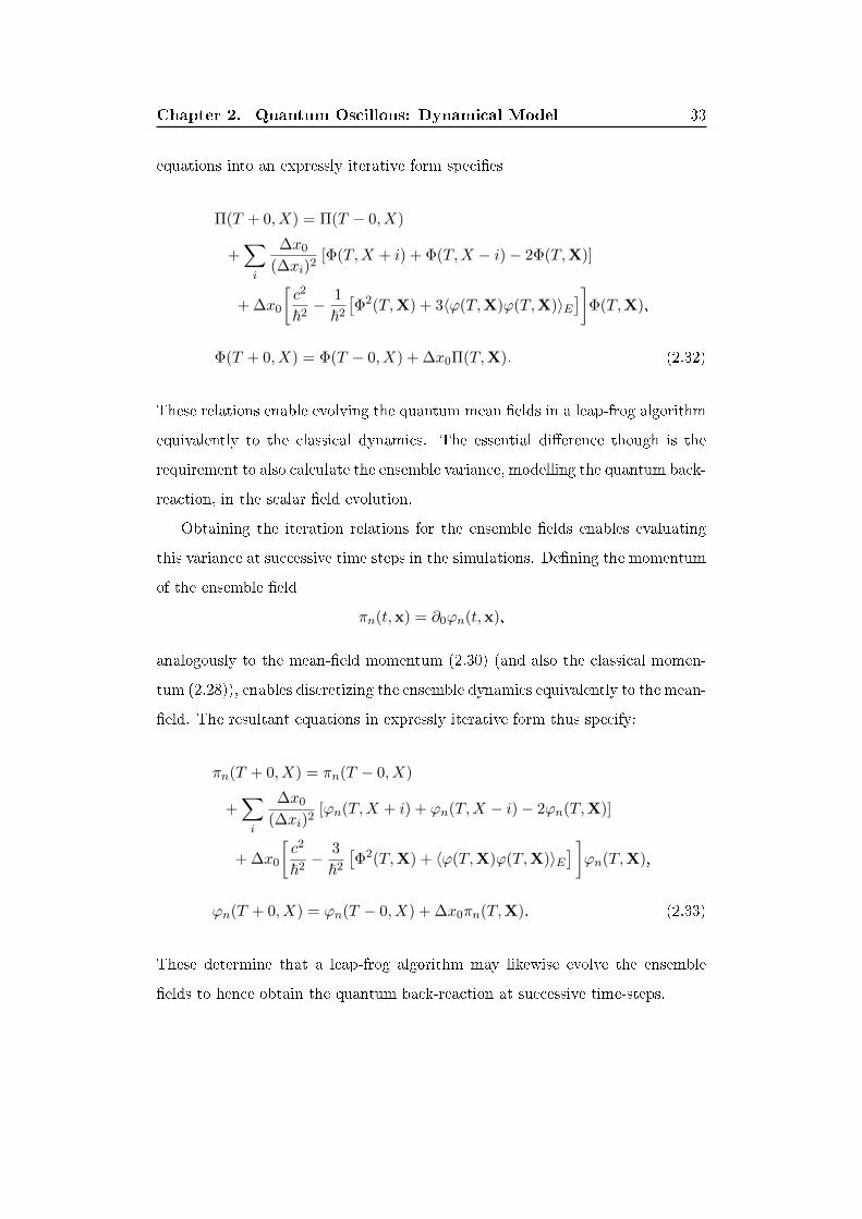
Obtaining the iteration relations for the ensemble �elds enables evaluating
this variance at successive time steps in the simulations. De�ning the momentum
of the ensemble �eld
πn(t,x) = ∂0ϕn(t,x),
analogously to the mean-�eld momentum (2.30) (and also the classical momen-
tum (2.28)), enables discretizing the ensemble dynamics equivalently to the mean-
�eld. The resultant equations in expressly iterative form thus specify:
πn(T + 0, X) = πn(T − 0, X)
+∑i
∆x0
(∆xi)2[ϕn(T,X + i) + ϕn(T,X − i)− 2ϕn(T,X)]
+ ∆x0
[c2
~2− 3
~2
[Φ2(T,X) + 〈ϕ(T,X)ϕ(T,X)〉E
] ]ϕn(T,X),
ϕn(T + 0, X) = ϕn(T − 0, X) + ∆x0πn(T,X). (2.33)
These determine that a leap-frog algorithm may likewise evolve the ensemble
�elds to hence obtain the quantum back-reaction at successive time-steps.

Chapter 3
Quantum Oscillons: Simulations
3.1 Parameter Choice for Numerical Simulations
Imposing throughout the dynamics natural units of ~ = c = 1 simpli�ed the
numerical implementation. This fully sets the evolutionary scales in the trans-
formed, classical system. The single ratio in the potential parameters remains to
uniquely determine the perturbation scale (equivalent to ~; see Section 2.2.3) in
the transformed, quantum system. This ratio, for simplicity, is also asserted to
satisfy λ/m = 1 throughout.
3.2 Numerical Code
Converting the iteration relations (2.29) for the classical �eld and the conjugate
momentum into a C code provided the basis for evolving the classical system.
The scalar �eld initialization simply involves setting the discretized �eld to the
value of the Gaussian ansatz (1.1) evaluated at the relevant lattice sites. These
values were computed using the standard library of C maths operations, with the
amplitude and radius provided through user input on intialization. The initial
conjugate momentum is likewise set simply to zero everywhere on the lattice.
Computing the classical evolution was accomplished, conveniently, using only a
34

Chapter 3. Quantum Oscillons: Simulations 35
serial code.
Implementing the iteration relations (2.32) of the quantum mean-�eld and
those of the ensemble �eld (2.33) also in a C code provided the basis for com-
puting the quantum evolution. The code applies the Open MPI libraries to
parallelize the evolution for the large number of ensemble �elds. Each processor
evolves the mean �eld and corresponding momentum to compute the ensemble
evolution, with a subset of the ensemble �elds and the corresponding momenta;
an MPI reduce command calculates the summation over the ensemble variables
to compute the ensemble variances in the dynamics.
The mean �eld initialization involved simply setting the values of the �eld
and the conjugate momentum across the lattice, equivalently to the classical
�elds. Forming the discrete equivalent to the mode expansion of the ensemble
�elds (2.24) enabled constructing the initial con�guration in wave-vector space.
The standard vacuum solution chosen for the initial mode functions (see Sec-
tion 2.2.4) determines the expansion at the initial time forms, simply, a Fourier
Transform. This was computed e�ciently using the FFTW routines. A standard
numerical method generates the randomly distributed numbers for the coe�-
cients in the expansion. This procedure employs a standard algorithm [73] to
generate random numbers uniformly distributed in the interval [0, 1). A further
routine subsequently converts these to Gaussianly distributed variables, where
the mean and variance for those coe�cients of a single k-value are set to satisfy
the constraints (see Section 2.3) on the ensemble. The e�ective independence
of the random numbers in the initial stage ensures the variance for coe�cients
of di�ering wave-vectors vanish, to impose also the independence of the distinct
k-components in the expansion (see again Section 2.3). A characteristic value in
the initial stage, importantly, determines the pseudo-random numbers generated;
hence, setting this distinctly on each processor ensures each processor contributes
a distinct set of �elds to the total ensemble.
Chapter 3. Quantum Oscillons: Simulations 36
3.2.1 Ensemble Size
The discretization of the system onto a square lattice of N = 256 ensured com-
putations over practical durations. Choosing the lattice spacing ∆x1 = ∆x2 =
∆x3 = 0.8 and time-step ∆x0 = 0.05 provided convergence in the evolved �elds.
These intervals, in particular, eliminated the (evidently unphysical) regrowth of
the �eld observed at larger values of these parameters for some of the initial
conditions.
A very large number of realizations M was necessary in this inhomogeneous
system: the results only converged aroundM = 60000 and above. For a lattice of
N = 256, this is a very small gain in computational operations time compared to
solving all the N2 = 65536 mode functions. This demonstrates the considerable
di�culty in computing the quantum e�ects on the oscillon dynamics
3.3 Choosing Initial Conditions
The space of the Gaussian initial pro�le (1.1) in the region A0 ∈ [−4, 4] and
r0 ∈ [0, 4] covers the main boundaries of the classical-oscillon basin of attraction
[42]. Each point in the region of negative, initial amplitude A0 corresponds, in a
non-trivial manner, to a point in the positive region. The initial con�guration, in
particular, evolves through half an oscillon to a maximum excursion, equivalent
to an initial Gaussian con�guration of opposite sign in the amplitude. This indi-
cates that studying only the positive range of A0 is su�cient to comprehensively
examine the quantum system in contrast to the classical case. Excluding also low
values of r0 and A0 where no oscillons are formed classically further constrains
the parameter space to study, and correspondingly reduces the necessary com-
putation time. The pairings (A0, r0) are thus chosen in the region A0 ∈ [0.25, 4]
and r0 ∈ [1, 4]. In particular, every pairing was constructed in this space, from
the minimum value of each range and increasing at discrete intervals of 0.25 up
to the maximum.

Chapter 3. Quantum Oscillons: Simulations 37
These initial con�gurations were then evolved on the square lattice of size
N = 256 with a converged ensemble of size M = 2562 = N2. Selected parameter
pairings were repeated on larger lattices of N = 384 and N = 512. The ensemble
size was also increased toN2 for each larger simulation, ensuring these maintained
the condition obtained on the smallest lattice for the ensemble to converge. For
�xed lattice spacing, the increasing lattice-size provided a test for �nite volume
e�ects; and for a decreasing lattice spacing to maintain �xed physical volume,
the set of larger simulations provided checks on resolution e�ects.
3.4 The Oscillon End-point
A convenient de�nition for the endpoint of the oscillon will be when the envelope
of the oscillations at the centre of the con�guration �rst crosses the classical
in�ection-point in the scaled potential.
The abrupt change in the dominant frequency of oscillations from below to
above the mass threshold provides an distinctive indication of the collapse of the
classical oscillon. This equivalently occurs where the amplitude of the con�gu-
ration is only slightly greater than the in�ection-point in the (classical) poten-
tial, closest to the vacuum around which the �eld oscillates; then the amplitude
rapidly decreases. (For the details on the eventual decay, see Section 1.2.2). Ex-
amining the �eld in real space provides a more convenient measure to determine
the �nal collapse � without the need to complete a Fourier transform to examine
the frequency components present. Where the envelope of the (scaled) �eld at the
centre of the con�guration �rst ceases to extend further than the in�ection-point
in the (scaled) classical potential, and closest to the vacuum around which the
oscillations occur, will therefore provide a convenient de�nition for the endpoint
of the oscillon.
Applying the �eld scaling (2.4b) to the classical potential in the (unscaled)

Chapter 3. Quantum Oscillons: Simulations 38
action (2.1) yields
V (φ) ≡ −c2m4
2~2λφ2(t,x) +
m4
4~2λφ4(t,x) +
c4m4
4~2.
The in�ection-point φf of this potential in the scaled system may hence readily
be determined:d2
dφ2V (φ)
∣∣∣∣φf
= 0 ⇒ φf = ±√c2
3.
This implies φf = ±√
1/3 for the choice of natural units. For also the �eld con-
�guration oscillating around the positive vacuum (see section 2.1.3), the positive
value will form nearest the vacuum around which the con�guration oscillates and
thus de�ne the endpoint of the oscillon.
3.5 Typical Evolution Pro�les
A comparison of the core �eld-value from identical, Gaussian con�gurations (1.1)
in both the classical and quantum case in �gure 3.1 illustrates the typical evolu-
tion both inside (left) and outside (right) the basin of attraction.
The classical evolution inside the basin of attraction (top, left) settles into an
oscillon lasting beyond the simulation time; while outside the basin (top right),
the central value decays below the in�ection-point of the potential in under two
oscillations of the �eld.
In the quantum case, the initialization outside the basin of attraction evolves
almost identically to the classical system: no oscillon forms and the �eld decays
in only a few oscillations. The quantum back-reaction, thus, generates no sig-
ni�cant e�ect outside the basin of attraction. Comparing the evolution within
the basin of attraction, however, readily shows a distinctive change on including
the quantum e�ects. The oscillations in the classical case remain fairly constant
through the majority of the evolution and below the classical in�ection-point;
the quantum case, though, decays within a gently decreasing envelope until after

Chapter 3. Quantum Oscillons: Simulations 39
Figure 3.1: The time evolution of the centre of a con�guration with an initial
condition inside (left) and outside (right) the basin of attraction for the classical
(top) and quantum (bottom) oscillon, where the �eld amplitude is in units of√m2/λ. (A0, r0) = (2.25, 2.5) and (1.0, 1.5) respectively in the initial Gaussian
con�guration (1.1). The con�gurations oscillates around the positive vacuum
(black, dashed), and the change in amplitude to above the in�ection-point (red,
dashed) of the classical potential de�nes the endpoint of the oscillon.
approximately one hundred periods, the amplitude ceases to extend below the
classical in�ection-point.
These cases, for the particular choice of initial Gaussian con�guration, also
demonstrate a much larger decrease in the amplitude within than �rst two oscilla-
tions in the quantum system, compared to the classical case. The Gaussian form,
only an approximation to the oscillon con�guration causes an initial transient, in
both the classical and quantum system. This transient is relatively small in the
Chapter 3. Quantum Oscillons: Simulations 40
classical case illustrated; and, thus, con�rms the highly accurate approximation
of the Gaussian to the oscillon con�guration in the classical system. The compar-
atively larger, initial decay in the quantum case simply illustrates the Gaussian
con�guration forms a poorer approximation to the true oscillon in the quantum
system.
The quantum case, nonetheless, demonstrates that the e�ective Hartree ap-
proximation may yield long-lived, oscillon solutions. This con�rms certain Gaus-
sian con�gurations are su�ciently similar to these solutions to evolve into the
true oscillon-con�guration. The lifetimes of these oscillons are evidently much
shorter than in the classical case. Further, the manner of the eventual decay by
these quantum oscillons is distinctly di�erent: while the classical con�gurations
terminate in a sudden collapse (see Section 1.2.2 for a discussion), the quantum
oscillations gradually deceases in amplitude. No signi�cant change, in particu-
lar, occurs in the quantum evolution when the oscillation amplitude nears the
classical in�ection-point. This notably contrasts the collapse at this stage of the
classical oscillon, indicating that this classical value has no relation to the shape
of the e�ective, quantum potential.
The quantum oscillon also, notably decays towards the positive vacuum of
the classical potential: verifying that the renormalization procedure, although
only approximate, is adequate.
Several of the initial con�gurations in the quantum system generate an oscil-
latory envelope at a longer period, modulating the basic, underlying oscillations.
Simulations at the higher resolutions for a selection of such cases eliminated the
strong modulations (see �gure 3.2, left for an illustrative case). These artefacts
of the coarser lattice spacing (grey line, in the �gure 3.2) essentially vanished on
the increase in spatial resolution (blue line, in the �gure 3.2), to generate purely
oscillations around the positive vacuum (black, dashed line, in the �gure 3.2) at
an amplitude below the in�ection-point (red, dashed line, in the �gure 3.2) of the
potential . This revealed the endpoint of these oscillatory con�gurations to have
Chapter 3. Quantum Oscillons: Simulations 41
clearly occurred around the time when the �eld in even the coarsest simulation
�rst crossed the classical point of in�ection. Any distinctive appearance of com-
parably strong beats further to those explicitly examined were hence disregarded
as unphysical; and the end of oscillations considered to be where the �eld �rst
crossed the in�ection-point1.
A beat-frequency of shorter period and smaller amplitude than the evidently
unphysical instances also modulated the underlying oscillations in several in-
stances (see �gure 3.2, right for an illustrative case; the grey line shows the lower
spatial resolution). Evolving a set of these instances at the higher spatial resolu-
tions (blue line, in the �gure 3.2) demonstrated the beat-frequencies remained.
This type of beat-frequency notably also modulated the underlying oscillon in
several classical cases.
Beating of this type has been observed in previous, detailed examinations
of scalar �eld oscillons in similar contexts: formed in symmetric double-well
potentials, from Gaussian initial conditions [37, 43]2. A careful examination
demonstrated certain values of the radius in the initial pro�le (1.1) produce a
local resonance in the oscillon lifetime. Small deviations from such a resonant
radius generates the type of beating observed in the present quantum-simulations
[37].
This type of beating has also been found in the scalar �eld oscillons, evolved
from Gaussian initial conditions in the sine-Gordon potential [43]. The oscillons
forming in the SU(2)-gauged, Higgs system also demonstrate similar beating
dependent on the particular initial conditions [55].
1These strong beats arose at varied points in the parameter space of initial pro�les. Thestark emergence of the beat-frequency after initially evolving similarly to neighbouring points inparameter space, together with the peculiar nature of the beat-frequency in comparison to theevolution on the underlying oscillons was su�cient to distinguish the unphysical modulations.Completing the larger simulations to con�rm the beat-frequencies to be unphysical in everysuch case was prohibitively time consuming.
2An investigation of oscillons in an anti-symmetric, double-welled potential has also notedthe occurrence of these beat-frequencies [36].

Chapter 3. Quantum Oscillons: Simulations 42
Figure 3.2: Initial conditions illustrating the two, distinct classes of beat-
frequencies modulating the oscillon evolution where the �eld amplitude is in units
of√m2/λ. These oscillate around the positive vacuum-value (black, dashed) and
when crossing the in�ection-point (red, dashed), are considered to have decayed.
The choice of (A0, r0) = (2.5, 1.5) in the Gaussian initial condition (1.1) produces
the large-amplitude modulations of the oscillon (grey) on the coarser lattice spac-
ing. These entirely vanish (blue) for �xed volume, on reducing the lattice spacing.
This determines the large-amplitude modulations are purely lattice spacing arte-
facts. The initial choice of (A0, r0) = (2.5, 2.5) (right) demonstrates the smaller-
amplitude and shorter-period modulations of the oscillon (blue) for the coarser
lattice spacing. These remain qualitatively unchanged (although the frequency
changes slightly) on reducing the lattice spacing, with the volume �xed. This
type of beat-frequency also occurs in the classical evolution; this is illustrated
in the oscillon con�guration in �gure 3.1 (top, left), where the beat-frequency
is more pronounced than in the quantum illustration above. The examination
of this type of modulations in various, more detailed studies implies these beat-
frequencies are a physical, long-lived transient, resulting from the discrepancy
in the initial conditions to the true oscillon structure. These modulations also
include an unphysical component demonstrated in their change on reducing the
lattice spacing. This may be neglected though in the measurement of the oscillon
lifetime.
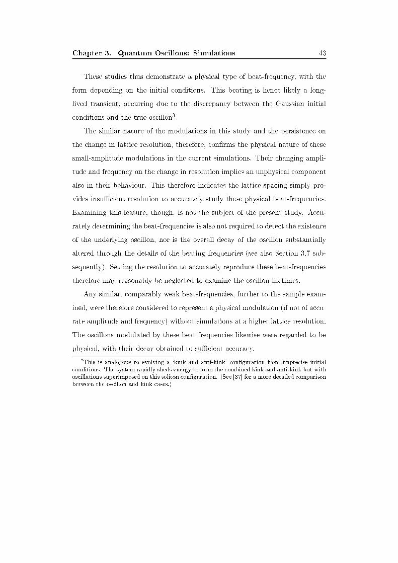
Chapter 3. Quantum Oscillons: Simulations 43
These studies thus demonstrate a physical type of beat-frequency, with the
form depending on the initial conditions. This beating is hence likely a long-
lived transient, occurring due to the discrepancy between the Gaussian initial
conditions and the true oscillon3.
The similar nature of the modulations in this study and the persistence on
the change in lattice resolution, therefore, con�rms the physical nature of these
small-amplitude modulations in the current simulations. Their changing ampli-
tude and frequency on the change in resolution implies an unphysical component
also in their behaviour. This therefore indicates the lattice spacing simply pro-
vides insu�cient resolution to accurately study these physical beat-frequencies.
Examining this feature, though, is not the subject of the present study. Accu-
rately determining the beat-frequencies is also not required to detect the existence
of the underlying oscillon, nor is the overall decay of the oscillon substantially
altered through the details of the beating frequencies (see also Section 3.7 sub-
sequently). Setting the resolution to accurately reproduce these beat-frequencies
therefore may reasonably be neglected to examine the oscillon lifetimes.
Any similar, comparably weak beat-frequencies, further to the sample exam-
ined, were therefore considered to represent a physical modulation (if not of accu-
rate amplitude and frequency) without simulations at a higher lattice-resolution.
The oscillons modulated by these beat-frequencies likewise were regarded to be
physical, with their decay obtained to su�cient accuracy.
3This is analogous to evolving a `kink and anti-kink' con�guration from imprecise initialconditions. The system rapidly sheds energy to form the combined kink and anti-kink but withoscillations superimposed on this soliton con�guration. (See [37] for a more detailed comparisonbetween the oscillon and kink cases.)
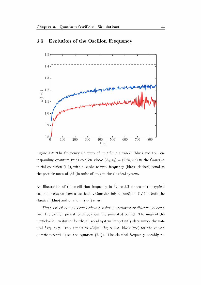
Chapter 3. Quantum Oscillons: Simulations 44
3.6 Evolution of the Oscillon Frequency
Figure 3.3: The frequency (in units of |m|) for a classical (blue) and the cor-
responding quantum (red) oscillon where (A0, r0) = (2.25, 2.5) in the Gaussian
initial condition (1.1), with also the natural frequency (black, dashed) equal to
the particle mass of√
2 (in units of |m|) in the classical system.
An illustration of the oscillation frequency in �gure 3.3 contrasts the typical
oscillon evolution from a particular, Gaussian initial condition (1.1) in both the
classical (blue) and quantum (red) case.
This classical con�guration evolves to a slowly increasing oscillation-frequency
with the oscillon persisting throughout the simulated period. The mass of the
particle-like excitation for the classical system importantly determines the nat-
ural frequency. This equals to√
2 |m| (�gure 3.3, black line) for the chosen
quartic potential (see the equation (2.1)). The classical frequency notably re-
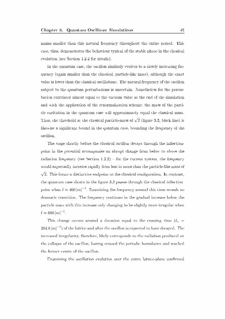
Chapter 3. Quantum Oscillons: Simulations 45
mains smaller than this natural frequency throughout the entire period. This
case, thus, demonstrates the behaviour typical of the stable phase in the classical
evolution (see Section 1.2.2 for details).
In the quantum case, the oscillon similarly evolves to a slowly increasing fre-
quency (again smaller than the classical, particle-like mass), although the exact
value is lower than the classical oscillations. The natural frequency of the oscillon
subject to the quantum perturbations is uncertain. Nonetheless for the pertur-
bation correlator almost equal to the vacuum value at the end of the simulation
and with the application of the renormalization scheme, the mass of the parti-
cle excitation in the quantum case will approximately equal the classical mass.
Thus, the threshold at the classical particle-mass of√
2 (�gure 3.3, black line) is
likewise a signi�cant bound in the quantum case, bounding the frequency of the
oscillon.
The stage shortly before the classical oscillon decays through the in�ection-
point in the potential accompanies an abrupt change from below to above the
radiation frequency (see Section 1.2.2) � for the current system, the frequency
would expectedly increase rapidly from less to more than the particle-like mass of√
2. This forms a distinctive endpoint to the classical con�guration. In contrast,
the quantum case shown in the �gure 3.3 passes through the classical in�ection-
point when t ≈ 460 |m|−1. Examining the frequency around this time reveals no
dramatic transition. The frequency continues in the gradual increase below the
particle mass with this increase only changing to be slightly more irregular when
t ≈ 600 |m|−1.
This change occurs around a duration equal to the crossing time (tc =
204.8 |m|−1) of the lattice and after the oscillon is expected to have decayed. The
increased irregularity, therefore, likely corresponds to the radiation produced on
the collapse of the oscillon, having crossed the periodic boundaries and reached
the former centre of the oscillon.
Examining the oscillation evolution over the entire lattice-plane con�rmed

Chapter 3. Quantum Oscillons: Simulations 46
Figure 3.4: The distance dpeak (in the scaled coordinates) from the origin to
the extrema of the oscillon evolution, evaluated when the core value Φ(t,0) is
also an extremum. This stage in the core evolution provides the time expectedly
corresponding to a (global) extrema of the oscillon con�guration. The extrema
of the oscillon are shown throughout the main evolution of the con�guration,
during the time t = 100 |m|−1 to t = 320 |m|−1 for the quantum case examined
in frequency space � evolving the Gaussian initial condition (1.1) where (A0, r0) =
(2.25, 2.5). This con�rms the oscillon remains relative static near to the origin
on the lattice compared to the initial, characteristic width of the pro�le.
that the change in the amplitude at the origin occurred in the peak value of the
oscillon. The �gure 3.4 shows the distance (in the scaled coordinates) from the
origin to the extrema in the oscillon, when the core-value Φ(t,0) is an extremum.
For a pure oscillon con�guration around the origin, the extrema of the core values
may precisely determine when the oscillatory con�guration also forms a global
extremum. The radiation (generated through the decay of the con�guration),
though, complicates the oscillon evolution on the periodic lattice. This radia-
tion expectedly contain much less energy than the oscillon throughout the main

Chapter 3. Quantum Oscillons: Simulations 47
evolution of the oscillations and, hence, are expected to only negligibly alter the
extrema of the oscillations. The waves, further, only infrequently cross the core of
the oscillon, on travelling through the periodic volume. This implies the radiation
may only infrequently alter the oscillon extrema, and likewise infrequently may
disrupt the correspondence between the core and global extrema4.) The extrema
of core value therefore provide a reasonable estimate of when the extrema in the
oscillations occur. Measuring the length from the origin to the extremum of the
oscillon in these instances thus determines any change in the central position
of the con�guration. This, importantly, involves no gradual shift, which could
potentially generate the gradual decrease noted in the core value throughout the
evolution. The position of the oscillation extrema, moreover, con�rm the central
extremum of the oscillon remains close to the origin on the lattice, compared to
the initial, characteristic width of the pro�le. This, hence, con�rms the core �eld
values (Φ(t,0)) provides a reasonable indication of the evolution of the oscillon
amplitude.
The continual increase in frequency at the origin (before the later irregu-
larities), therefore, genuinely characterizes the oscillon amplitude. This grad-
ual change without any distinctive indicator when the oscillon decays notably
matches the ambiguity in the endpoint de�ned through the �eld amplitude. The
oscillation envelope therefore provides a measure, equally suitable to any measure
involving the frequency, for de�ning the decay of the quantum oscillon.
4The radiative waves superimposed on the oscillon pro�le may alter the resultant extrema ofthe oscillations, and also disrupt the correspondence between the core extrema and the oscillonextrema. This radiation will begin to a�ect central region of the oscillon pro�le around the originafter approximately the lattice crossing time. The seeming peaks in the distance (dpeak) to theextrema, after this time likely correspond simply to waves crossing the oscillon and consequentlyshifting where the peak in the oscillon con�guration occurs. While the energy in the radiationis much less than the energy in the oscillon, the wave amplitude correspondingly will be muchsmaller than the oscillon amplitude. This, therefore, assures the neglect of the waves providesa reasonable approximation throughout the majority of the oscillon evolution. The much largersize of the lattice compared to the oscillon radius, also, indicates the radiation will cross theoscillon only infrequently. This further validates the neglect of the waves on the extrema of theoscillations. The low crossing frequency likewise implies the waves only infrequently alter thecore value and hence assures the infrequent disruption of the correspondence between the coreand the global extrema of the con�guration.

Chapter 3. Quantum Oscillons: Simulations 48
3.7 Determining Oscillon Lifetimes
The categorization of the evolution types and the de�nition of the oscillon end-
point allow a consistent determination of the oscillon lifetimes over both the
classical and quantum initialization space.
An illustration of a classical oscillon in �gure 3.1 (top, left) shows the typical
stability of the oscillations around the positive (broken-phase) minimum over the
simulation. The envelope never decreases below or nears the in�ection-point; and
hence a slight modi�cation in the precise de�nition of the endpoint creates no
change in the detection of the oscillon.
The characteristic quantum-oscillon in �gure 3.1 (bottom, left) shows the
gradual decay in amplitude. This implies the precise lifetime will depend on the
de�ned �eld-value for the endpoint. Nonetheless, a slight shift in the value de�n-
ing the decay point only slightly alters the lifetime due to the gradual decrease
of the envelope. The altered endpoint would, further, produce a change to the
lifetime similarly in each case. This hence assures the di�erences between the
lifetimes would remain largely unaltered.
The de�nition of the oscillon endpoint is thus robust for both the classical
and quantum systems.
Additionally, the distinctive variants in the quantum system demonstrated
(in the previous section) that the strong beat-frequency distinguishes that the
oscillations have decayed in actuality when the envelope �rst crosses below the
classical point of in�ection. This endpoint importantly is largely unchanged
(�gure 3.2, left) in the high-resolution simulations eliminating the unphysical
modulation. The �rst modulated oscillation at an amplitude below the classical
point of in�ection thus provides a reliable de�nition of the endpoint in such cases.
Those cases where a small, physical beat-frequency modulates the oscillations
equally signify the decay to arise when the envelope �rst decreases below the
classical in�ection-point (�gure 3.2, right). Again, the position where the net,

Chapter 3. Quantum Oscillons: Simulations 49
modulated �eld-amplitude �rst decreases below this threshold suitably de�nes
the endpoint.
These de�nitions, notably, in the case of beat-frequencies involve the net,
modulated �eld, although the instant where the envelope decreases below the
in�ection may de�ne an equally valid endpoint. This poses an ambiguity in
the oscillon lifetimes evaluated through the alternative methods. These variable
de�nitions (in each case) though involved only minor di�erences compared to the
computed lifetimes.
The changing in the beat-frequency on varying the lattice spacing also may
alter the instant when the net, modulated-�eld amplitude decreases below the
in�ection point. These di�erences in each cases examined at di�ering lattice
spacings, though, were negligible compared to the oscillon lifetime.
This consistency in the obtained values (at di�ering lattice spacings and for
distinct de�nitions) therefore ensures the choice to examine the net, modulated
�eld forms a robust quantity to determine the lifetime.
These small-amplitude beat-frequencies further generate oscillations of the
net �eld around the in�ection classical point over a period. This creates an am-
biguity in precisely de�ning the endpoint of the oscillon. The choice to de�ne the
�rst instant when the oscillation amplitude decreases below the in�ection-point
to be the endpoint thus creates a systematic error compared to the alternative
crossings of either the net �eld or the envelope. Nonetheless, the chosen crossing
provides consistency in the de�nition over the entire parameter-space, and the
variation from choosing the alternative points for the cases examined (compared
to the calculated lifetime) were minor.
3.8 Mapping the Attractor Basin
Applying the de�ned endpoint to the oscillons over the parameter space of Gaus-
sian initial conditions (1.1) reveals the classical (�gure 3.5) and quantum (�gure

Chapter 3. Quantum Oscillons: Simulations 50
3.7) basin of attraction.
Figure 3.5: The lifetime of classical oscillons projected onto the parameter space
of Gaussian initial conditions (1.1).
The classical case shows oscillons arise from the Gaussian initial conditions in
two main regions: over a broad section of the positive-amplitude con�gurations
and in a narrower range of the negative amplitudes. These are separated by
a band of instability failing to generate oscillons around a zero amplitude. A
minimum initial width, thus, bounds these regions, de�ning the minimum size
(and corresponding minimum-energy) necessary for generating an oscillon.
These classical oscillons last at least O(104 |m|−1) and have not decayed be-
fore the end of the simulation, con�rming previous observations [42�44, 46, 52].
This bifurcated attractor basin presents a potentially misleading illustration.
In actuality, the oscillons of a positive initial amplitude oscillate to values above

Chapter 3. Quantum Oscillons: Simulations 51
the vacuum, corresponding to a negative-amplitude initialization (see Section
2.1.3); and vice-versa. The initial con�gurations in the positive and negative
regions thus form � although in a non-trivial manner � related pairings.
Examining the energy of the Gaussian con�gurations, at least in the classical
case, o�ers a method to establish an approximate relation between the positive
and negative-amplitude initial conditions. Constructing the classical Hamiltonian
of the action (2.1) and applying the �eld scaling (2.4) yields
H(t) =m2
λ
∫d2x
[1
2
∑µ
(∂µφ(t,x))2 − c2
2~2φ2(t,x) +
1
4~2φ4(t,x) +
c4
~2
]. (3.1)
Substituting the initial, Gaussian con�guration (1.1) and the choice of zero mo-
mentum into the classical Hamiltonian and evaluating the integral hence deter-
mines
H =1
2A2
0r20 −
1
3A3
0r30 +
1
16A4
0r40. (3.2)
This provides a precise expression of the initial energy for the classical con�gura-
tion. The reasonably accurate approximation of the Gaussian to the true oscillon
con�guration (see Section 1.2.1 and 3.5) implies that this expression also remains
a close approximation to the energy of the subsequently evolving oscillon at the
maxima of the amplitude, where the �eld momentum again equals zero. Only
a small change in the radius of the oscillons typically occurs throughout their
evolution [36, 42]. This therefore indicates con�gurations of a positive, initial
amplitude A0 may oscillate to an approximately Gaussian con�guration of an
identical radius but a negative A0 at the maximum of the oscillation, where the
maximum amplitude corresponds to a con�guration of equal energy to the initial
Gaussian. The con�gurations of a negative initial amplitude may, likewise, evolve
to a minimum amplitude of equal energy to the initial con�guration. This, thus,
indicates an equivalence in the classical evolution of the positive and negative
initial amplitudes.
Examining the contours of equal energy in the parameter space of the Gaus-
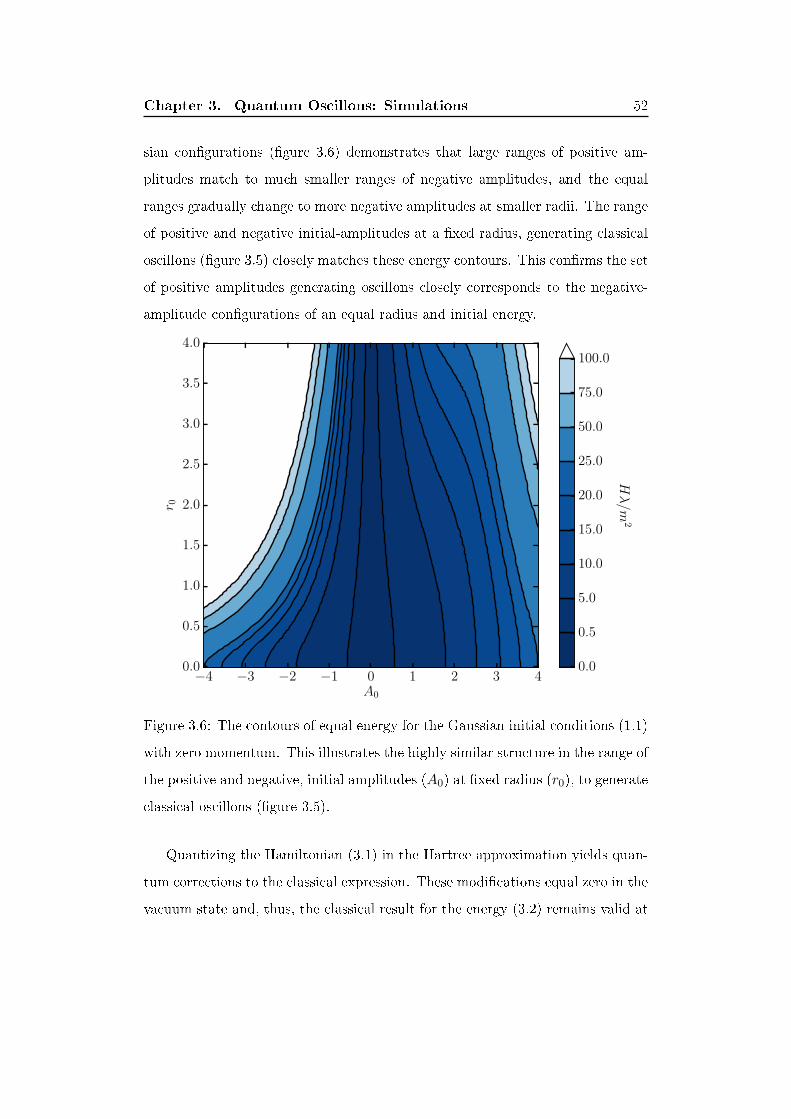
Chapter 3. Quantum Oscillons: Simulations 52
sian con�gurations (�gure 3.6) demonstrates that large ranges of positive am-
plitudes match to much smaller ranges of negative amplitudes, and the equal
ranges gradually change to more negative amplitudes at smaller radii. The range
of positive and negative initial-amplitudes at a �xed radius, generating classical
oscillons (�gure 3.5) closely matches these energy contours. This con�rms the set
of positive amplitudes generating oscillons closely corresponds to the negative-
amplitude con�gurations of an equal radius and initial energy.
Figure 3.6: The contours of equal energy for the Gaussian initial conditions (1.1)
with zero momentum. This illustrates the highly similar structure in the range of
the positive and negative, initial amplitudes (A0) at �xed radius (r0), to generate
classical oscillons (�gure 3.5).
Quantizing the Hamiltonian (3.1) in the Hartree approximation yields quan-
tum corrections to the classical expression. These modi�cations equal zero in the
vacuum state and, thus, the classical result for the energy (3.2) remains valid at
Chapter 3. Quantum Oscillons: Simulations 53
the initial time in the quantum case. The quantum corrections in the subsequent
evolution, in general, though are non-zero, and thus the classical result is inval-
idated at later times. (Calculating the corrections would involve obtaining the
correlators of the quantum perturbation and hence poses an equivalent di�culty
to the challenge of solving the quantum dynamics. Neither is a suitable analytic
approximation readily attainable to examine the quantum corrections.) This
purely quantum modi�cation, thus, eliminates the simple, classical equivalence
of each initial, positive-amplitude con�guration to the Gaussian of correspond-
ing negative amplitude but equal energy, and vice versa. The stronger di�erence
between the Gaussian and the true oscillon con�guration (Section 3.5) in the
quantum case, further, indicates that the energy evaluated for the Gaussian �eld
con�guration (1.1) provides a poorer estimate of the actual energy on the evolv-
ing the quantum oscillon. This again invalidates the simple, classical equivalence
between the evolution of the positive and negative amplitudes. The positive, ini-
tial amplitudes generating oscillons, nonetheless, evolve to a state of amplitude
above the vacuum, equal to a negative, initial amplitude (see Section 2.1.3), and
vice versa. A careful examination of the initial maximum and minimum (imme-
diately subsequent to the initial transient) might enable more precisely matching
the positive and negative initial amplitudes evolving to equivalent con�gurations.
This is unnecessary though for examining the quantum e�ects on the oscillon life-
time. The assured equivalence in the evolution of the positive and negative initial
amplitudes implies that the positive initial conditions, thus, incorporate the en-
tirety of quantum oscillon-evolution. Examining the positive region, therefore,
provides a su�cient range of amplitude to fully assess the quantum e�ects on the
oscillon lifetime.
The �gure 3.7 illustrates the quantum equivalent to the classical evolution in
the �gure 3.5, except across the restricted range in Gaussian initial conditions.
Oscillons in the quantum case arise over a largely similar region of the Gaussian
parameter space to those in the classical case (white lines, 3.7). In particular,

Chapter 3. Quantum Oscillons: Simulations 54
Figure 3.7: The lifetime of quantum oscillons projected onto the parameter space
of Gaussian initial pro�les (1.1). The white contours indicate the classical basin.
a band for amplitudes below a value around the in�ection-point generates no
oscillons; and a minimum radius also bounds the attractor-basin threshold. The
quantum perturbations, though, alter the precise bounds of the attractor basin
from the classical case. Most signi�cantly also, these oscillons, subject to the
quantum �uctuations, persist for considerably less time than the classical coun-
terparts: typically ending before O(103 |m|−1).
3.9 Conclusion
These results have shown the �rst quantum, dynamical simulations of oscillons.
These demonstrated that (with ~ = c = λ/m = 1) the quantum �uctuations
signi�cantly reduced oscillon lifetimes compared to the classical case. Further,
the decay under the quantum evolution occurs gradually, without distinctive

Chapter 3. Quantum Oscillons: Simulations 55
change in either the oscillation amplitude or frequency. This markedly contrasts
the classical oscillons. The detailed decay-process, though, remains unclear.
Conducting the comparison of the Gaussian attractor basin (for positive, ini-
tial amplitudes) showed that both the classical and quantum oscillons result in a
similar region of the parameter space � despite the distinctly di�ering evolution
and lifetimes. This indicates that, at least initially, the purely classical terms
in the potential � the terms present in both cases � dominate the formation of
oscillons. The stronger, initial decay in the amplitude of the quantum oscillons,
in contrast to the classical case, implied that the quantum back-reaction alters
the oscillon con�guration. Those con�gurations creating an oscillon, thus, react
to the quantum �uctuations. The progression after the initial transient to a com-
paratively stable phase, similar to the classical case, indicates that the classical
components of the potential dominate during this early phase of the evolution;
and the quantum �uctuations predominantly alter the later decay.
These quantum, dynamical simulations have been accomplished through ap-
plying the inhomogeneous Hartree approximation to solve the equations of motion
on a two-dimensional lattice. The construction of a statistical ensemble of �elds
was used to approximate the quantum correlators. These �elds are of the form
ϕn(t,x) =
∫d2k
(2π)2
[ck,nfk(t,x) + c∗k,nf
∗k(t,x)
], (3.3)
where the random numbers ck,n are chosen to reproduce the ladder-operator
correlators. The statistical mean of these ordinary numbers in e�ect replaces
the quantum average of the operators in the system. This hence determines
the variance of the ensemble �elds may replace the quantum correlators in the
dynamics:
〈ϕn(t,x)ϕn(t,x)〉E −→ 〈δφ(t,x)δφ(t,x)〉. (3.4)
Requiring each ensemble �eld to satisfy the mode dynamics (2.14) implies that
the constructed equation e�ectively evolves all the mode functions simultaneously
Chapter 3. Quantum Oscillons: Simulations 56
within the ensemble �eld. This ensures the variance of the ensemble �elds (with
the correct choice of the random numbers) corresponds to the quantum correlator
at all times. Establishing this equivalence, thus, forms the basis to examine the
quantized dynamics through the ensemble �elds.
The ensemble method, in principle, involves in�nitely many �elds for a pre-
cise equivalence between the quantum correlator and the statistical variance. In
practice, the use of a �nite ensemble size to accurately approximate the exact
quantum value o�ered the possibility to reduce the computational requirements
compared to evolving the mode functions. This method, though, for the quantum
dynamical simulations of the oscillon provided negligible computational bene�t.
The tests demonstrated the need for an ensemble size of M = 60000 to obtain
su�cient convergence in the �elds. On the square lattice of N = 256 point, this
was only marginally fewer �elds than the N2 = 65536 modes required in the
mode function method.
This result contrasts the use of the ensemble method in the quantum, dy-
namical simulations of Q-Balls [13] in 3 + 1D. These only required an ensemble
size less than one tenth of the total modes on the lattice. The oscillon case like-
wise contrasts the 2 + 1D simulations of domain walls [8]. These also required a
consistently smaller ensemble size compared to the mode functions. This discrep-
ancy demonstrates the exceptionally di�cult nature of examining oscillons in the
quantum regime. The strongly inhomogeneous nature of the oscillon likely cre-
ates the need for a large ensemble to accurately examine the quantum dynamics
of the (highly non-perturbative) con�guration. Obtaining the oscillon lifetimes
also involved the examination of the �eld evolution directly, without any averag-
ing � unlike in the domain wall case � to potentially help reduce any statistical
�uctuations. This might necessitate considerable accuracy in the approximation
of the ensemble to the quantum correlators, and accordingly requires a large
ensemble size.
The comparable size of the ensemble to the number of modes notably matches

Chapter 3. Quantum Oscillons: Simulations 57
the results in 1 + 1D simulations applying a statistical ensemble to compute the
quantum, fermion correlators [74]. This may indicate that the low dimension-
ality of the oscillon simulations also results in the ine�ciency of the ensem-
ble method for examining the quantum scalar-�eld. Implementing the ensemble
method might therefore provide a signi�cant increase in the computational e�-
ciency for similar investigations in three and higher dimensions.

Chapter 4
Introduction: Fermions
The preceding discussion and the detailed investigation into oscillons have pri-
marily concerned bosonic �elds. A comprehensive understanding of quantum
�elds though must also incorporate fermionic degrees of freedom.
Their inherently quantum nature prevents any classical approximation pro-
viding an accurate treatment, and accordingly analysing fermions is problematic.
Perturbation theory provides a powerful technique for understanding fermionic
�elds and ultimately establishing their central role within the Standard Model of
particle physics: Quantum Electrodynamics provides a principal component in
the current, foremost theory for explaining fundamental physics [75].
Various contexts of potentially fascinating and relevant consequence involve
fermions in an inherently non-perturbative regime. The consequent e�ects in
several important cases will be examined in this chapter, where the discussion
will consider the results in relation to the methods for solving the systems. In-
corporating both the quantum and the non-perturbative nature in the analysis
poses a considerable challenge. The examined applications of these methods
though demonstrate the importance of solving such di�cult systems, to obtain
a comprehensive and accurate understanding. An overview of the techniques
for examining fermionic systems will presently form the introductory discussion
to the various applications. These methods, in particular, will ultimately be
58
Chapter 4. Introduction: Fermions 59
exploited for analysing quantum tunnelling in an idealized laboratory scenario.
4.1 Solving Fermion Dynamics
The Dirac equation provides the basis for understanding fermions:
(γµDµ +
mc
~
)Ψ(x) = 0. (4.1)
This strikingly simple equation, remarkably, determines various important fea-
tures of fermions [76]. The equation may be constructed essentially on attempting
to obtain �eld dynamics also satisfying relativistic, Lorentz invariance [75, 77].
This condition producing the Dirac equation inherently determines the spin-half
nature of fermions [77]. The equation, importantly, also implies the existence of
the negative-energy, anti-particle positrons [78].
Adding a fermion-gauge interaction through
iq
~Ψ(x)γµAµ(x)Ψ(x)
into the action for the Dirac equation, together with the terms for classical
electromagnetism, produces the standard, quantum electrodynamics Lagrangian.
This equally forms a remarkably simple basis for the analytical power to describe
nearly all phenomena across macroscopic scales to 10−3cm [75]. The (three-
point) gauge-fermion interaction yields an inherently two-point correlator in the
equations of motion and correspondingly the mode function method o�ers a con-
venient method to evaluate this contribution [75, 79]. This procedure (in contrast
to the bosonic case) enables accurate evaluation of the fermionic e�ects without
further approximation.
Implementing the mode expansion on the lattice, equivalently to the bosonic
case, involves a summation over the discrete mode space. This process likewise
for the fermions, on a d-dimensional lattice of NL sites in each direction, entails

Chapter 4. Introduction: Fermions 60
evaluating the functions for each of the NdL mode values in the summation. The
problem is also moderately worsened in the fermionic case since the fermionic �eld
comprises a four component spinor and the modes include both the particle and
anti-particle contributions: creating a factor of eight in the total �eld components
required for evolution. This NdL scaling equivalently to the bosonic case therefore
implies that any case with d > 1 requires increasingly extensive computational
resources.
Canonical quantization imposes an anti-commutation relation on the fermion
�elds. The ladder operators, on forming the mode expansion subsequently, en-
capsulate the anti-commutation structure; and, hence, the mode analysis to eval-
uate the correlators intrinsically also incorporates the anti-commuting properties.
Simply substituting a single ensemble for the fermionic operator equivalent to the
bosonic case, consequently, fails to reproduce the fermionic correlator. This sin-
gle ensemble crucially involves only ordinary, commuting numbers excluding the
possibility to represent the anti-commuting nature. Creating a second ensemble
may resolve this problem [74, 80, 81]. The �elds explicitly satisfy
ΨM,c(x) =
√~c2Vx∑s
∫d3k
(2π)3
(ξk,s,cψ
(U)k,s (x) + ζk,s,cψ
(V )k,s (x)
),
ΨF,c(x) =
√~c2Vx∑s
∫d3k
(2π)3
(ξk,s,cψ
(U)k,s (x)− ζk,s,cψ
(V )k,s (x)
),
where {ψ(U)k,s } and {ψ
(V )k,s } are the modes with {ξk,s,c} and {ζk,s,c} independent
sets of (complex) random numbers, and Vx is the total, real-space volume. These
integrands, importantly, di�er only in the plus or minus sign; these very simi-
lar counterparts are termed the �male� and �female� �elds. The plus and minus
signs ensure computing combinations of both the male and female �elds may
yield an integrand involving a sign di�erence between the term in the ψ(U)k,s and
that in the ψ(V )k,s for a �xed wavevector. This, importantly, reproduces the struc-
tures resulting on applying the anti-commutator relation of the ladder-operators,

Chapter 4. Introduction: Fermions 61
unattainable if only using a single ensemble.
A judicious choice of the random numbers (as in the the bosonic case) may,
hence, ensure these combinations of male and female �elds precisely reproduce
the quantum correlator. Choosing the random numbers in particular to form a
Gaussian random distribution proportional to the ladder anti-commutators [74,
80, 81] implies
〈T ˆΨ(x)OΨ(x)〉 = −〈ΨM (x)OΨF (x)〉E = −〈ΨF (x)OΨM (x)〉E ,
for O an arbitrary operator. (The male and female �elds thus notably perform an
interchangeable role, and in practice the quantum correlator may be constructed
through the average of these symmetric expectations.) These Gaussian distribu-
tions create the evident di�culty, also present in the bosonic case, of requiring
an in�nite ensemble; and this problem is worsened in the fermionic case through
the additional requirement to evolve two ensembles, both in�nite. The method
in practice, though, equivalently to the bosonic case, might reproduce the cor-
relators to a su�cient accuracy when the total number of both the male and
female �elds is smaller than the mode space: thus, reducing the computational
requirements required, compared to the standard, mode evolution.
This ensemble method for fermions has demonstrated an exceptional e�ec-
tiveness in examining the the fermionic back-reaction on classical, scalar-�eld
oscillons [80]. The computations uncovered an exponential decay in the total
oscillon-number starkly contrasting the slow, power law decay in the absence of
fermions for the ensemble size only around one hundredth of the total lattice
sites.
A 1 + 1D system to examine charge-parity (CP) violation within an Abelian-
Higgs model carefully determined the variation in ensemble size to produce con-
vergence in the results only for an ensemble larger than the total lattice-sites
[81]. This analysis though proved the reliability of the method for examining CP
Chapter 4. Introduction: Fermions 62
violation � the fermion number accurately approximating the dynamical Chern-
Simons number characterizing the gauge �elds and thus satisfying the theoretical
expectation. A further study examined CP-violation in a 3 + 1D system for the
SU(2)-Higgs �elds [74]. The ensemble method provided su�cient accuracy to
examine the particle production for the ensemble sizes typically around a third
to a tenth of the total sites (N3L) on the lattice.
These systems thus demonstrate the potential for the ensemble method for
fermionic �elds to detriment computational e�ciency in 1 + 1D but provide a
bene�t in 3 + 1D. The signi�cant enhancement for the case involving fermionic
back-reaction onto oscillons further examined a 2 + 1D space. This thus further
supports the ensemble method for fermions provides bene�t only in higher than
1 + 1D.
4.2 Fermions on the Lattice
Naively discretizing the fermion dynamics onto the lattice creates the familiar
�doubler problem�. This phenomenon involves 24 = 16 fermion species � each
with two charges and two spin states � occurring on the lattice and these unphys-
ical particles potentially contributing pronounced lattice-artefacts. A variety of
methods may help to alleviate the spatial doublers including most notably Wilson
fermions [82] and also staggered fermions [83, 84] or Ginsparg-Wilson fermions
[85]. The Wilson Fermion methodology may, equivalently, ameliorate the tempo-
ral doublers; a judicious choice of the initial conditions with a su�ciently small
time-step, alternatively, may suppress the presence of temporal doublers [82, 86].
This problem of doublers on the lattice results, essentially, through the fer-
mion evolution involving the solutions to a �rst-order di�erential equation. The
basic origin of the doublers may be most readily examined on considering a
homogeneous, �rst-order di�erential equation of a one-dimensional function:
∂x1f(x1) = 0.
Chapter 4. Introduction: Fermions 63
Each component of the fermionic spinor notably satis�es (dependently) an equa-
tion of this type on applying the Dirac equation (4.1) for masless fermions
(m = 0) in either a homogeneous system or, equivalently, in the static state
of a 1 + 1D system.
This �rst-order equation, in the continuum, implies only a single, possible
solution, where f equals a constant. Forming the standard, symmetric1 dis-
cretization of the �rst-order derivative (see equation 2.27) yields
f(X1 + 1)− f(X1 − 1)
∆x1= 0.
This forms the equivalent �eld equation on the lattice to the continuum, �rst-
order equation. The lattice expression, importantly, involves the �eld evaluated,
rather than at consecutive intervals, two intervals apart. This, hence, implies the
even intervals may satisfy one solution, f(2n1∆x1) = C1 and the odd sites may
satisfy an independent solution f((2n1 + 1)∆x1) = C2, for integers n1 and where
C1 and C2 are constants. The solution matching the continuum result, thus,
reproduces the continuum dynamics on the lattice, while the alternative solution
forms a solution unique to the lattice. This result, an artefact of the discretiza-
tion, thus, encapsulates the origins of the doubler in the fermionic system.
Examining the fermionic propagator and the corresponding excitation-energy
spectrum, more formally, demonstrates the existence of these doublers on the
lattice in 3 + 1D (for a detailed discussion see for instance [86]). Forming the
naive discretization of the Dirac equation (4.1) on the lattice may yield the free-
1An asymmetric approximation to the �rst derivative may also be formed, involving functionthe �eld at the chosen point f(X1) and either of the consecutive intervals: f(X1+1) or f(X1−1).Using this asymmetric form would, importantly, invalidate the basic explanation for doublers.The symmetric derivative, though, provides both the more accurate discretization on the latticeand also retains the isotropic nature of derivative through not incorporating any directionalpreference. This therefore forms the more desirable choice of discretization on the lattice. Theexamination of the symmetric form, moreover, provides an intuitive insight the basic structuresin the lattice theory generating the doublers. Examining the fermionic propagator, may morerigorously, demonstrate the existence of the doublers � this process is outlined, subsequently,in the case of fermions in 3 + 1D.

Chapter 4. Introduction: Fermions 64
fermion propagator in wave-vector space:
S(K) =
mc~ − i
∑µ
1∆xµ
γµ sin(Kµ∆xµ)(mc~)2
+∑
µ1
(∆xµ)2 sin2(Kµ∆xµ), (4.2)
for the fermion mass m and the wavevector K (with components Kµ) on the
lattice. Subsequently integrating the temporal wave-vector component explic-
itly yields the time dependency of the propagator. The resultant expression
includes two terms: both the usual time-evolution factor in the continuum and
a further term involving a rapidly oscillating factor (−1)t. This indicates the
presence of the second temporal-species on the lattice and the corresponding
rapid-oscillations in time. These oscillations in practice are typically evident in
the physical variables oscillating between extrema on successive timesteps � and
superimposed on the physical variation corresponding to the continuum evolu-
tion.
Setting the initial conditions to purely the discrete equivalent of the con-
tinuum con�guration ensures initially only the physical particles are present.
Ultimately, energy transfer may create the temporal doublers in system. Typ-
ically though for su�ciently small lattice-spacings, this doubler production is
heavily suppressed throughout the simulation and hence prevents the distinctive
oscillatory disturbance. This method, accordingly, will provide the mechanism
to prevent the temporal doublers within the subsequent computations.
The integration of the propagator (4.2), further, determines the energy spec-
trum of the naively discretized Dirac equation:
sinh
(ω∆x0
c
)= ∆x0
√(mc~
)2+∑i
sin2(Ki∆xi).
A particle state corresponds to a local minimum in the energy surface. The
spectrum, hence, implies that the naively discretized system involves 23 fermion
species. These further subdivide into those corresponding to the usual time
Chapter 4. Introduction: Fermions 65
variation in the continuum and the temporal-doublers. This, hence, amounts to
the �nal count of 24 fermion species in the naively discretized system. The 23
spatial variants, signi�cantly, include both particles with a mass corresponding
to those particles in the continuum theory but also additional particles, forming
the spatial-doublers in the naive discretization.
Implementing instead the Wilson fermions on the lattice will provide the
method to eliminate the spatial doublers in the subsequent simulations. This
procedure involves adding a Wilson term to the action:
1
c
∫cdtd3x
rw2
∑i
∆xiΨ(x)DiDiΨ(x),
where DiΨ(x) = (∂i − (iq/~)Ai(x)) Ψ(x). This additional term notably reduces
to zero in the continuum limit to recover precisely the Dirac fermions; but on
the lattice, the term importantly modi�es the energy spectrum. Setting the
Wilson parameter rW = 1 essentially modi�es the higher momentum modes to
entirely remove the energy degeneracy and produces a single energy-minimum
corresponding to the continuum particle state. Choosing the Wilson parameter
rW < 1 may still create doublers corresponding to local energy minima (for a
detailed examination in 1 + 1 see also [76]); but if the modi�cation to the energy
spectrum increases the energies to high values this may help prevent exciting
these unphysical particles.
The spatial doublers equivalently to the temporal doublers generate spatial
oscillations in the physical observables on the lattice-spacing scales. Selecting
the Wilson parameter to adequately limit these oscillations in practice provides a
su�cient method to choose the parameter value. The absence of the characteristic
spatial oscillations therefore will su�ciently validate the chosen rW < 1 in the
subsequent simulations.
Chapter 4. Introduction: Fermions 66
4.3 Quantum Tunnelling
Examining the potential for quantum interactions to generate tunnelling of a par-
ticle through a potential barrier will form the essential context for implementing
numerical simulations of fermions in the subsequent sections. Tunnelling through
a potential barrier, in general, is a distinctly quantum phenomenon. The paradig-
matic case occurs in quantum mechanics, for a particle classically con�ned by a
potential barrier of �nite strength [87]. Where the energy of the particle is less
than the potential barrier, the particle classically is unable to move through the
barrier. In quantum mechanics though, the location of the particle is determined
through a wavefunction satisfying the Schrödinger equation. The wavefunction
decays through the barrier but is non-zero, implying a �nite probability for the
particle to traverse the barrier. Continuity at the boundaries further constrains
the wavefunction in the free space, outside the classically allowed region to be
�nite. The result hence implies a �nite probability to observe the particle within
the classically forbidden region. This process occurs also in accordance with
the Heisenberg Uncertainty Principle [87]. The constraint on the uncertainty in
measuring both the position and the momentum of the particle precludes a zero
probability to detect the particle; and thus determines the quantum system to
involve this �nite probability for observing the particle to have tunnelled through
the barrier. This phenomenon historically has explained radioactive decay [88,
89]; while also being applied practically in scanning tunnelling microscopes [90]
and for everyday use in solid state memory [91].
Quantum �eld theory enables a second type of tunnelling. The quantum in-
teraction between di�erent particle species may enable the one kind to transmute
into the second in an oscillatory species-mixing. A barrier may form a classically
impenetrable obstruction to the original species while the second species may
freely travel through this region. The generated particle having traversed the
barrier may revert to the original species through the continuing quantum os-

Chapter 4. Introduction: Fermions 67
cillations, and thus produce the tunnelling into the classically forbidden region.
This process forms the basis of the standard �light shining through a wall experi-
ments� typically proposed to detect either axions [92, 93] or similar light particles
within the laboratory [94, 95].
The quantum �eld theory interactions enable a further mechanism for the
particles to tunnel through a barrier. This generalization to the preceding mech-
anism involves the original species transforming through pair-creation into a sec-
ond species able to travel through the barrier. These pair-created particles, on
passing through the barrier, subsequently annihilate to (re-)create the original
species. This �tunnelling of the 3rd kind� thus forms a distinct and purely quan-
tum mechanism for particles to traverse a barrier [96�98].
The process may occur in a (generic) non-local, e�ective theory, where the
tunnelling predictions hence form a test of the model. This may be the case,
in particular [96], where an electromagnetic �eld traps a particle in a particular
state, but an excited state of the atom may freely traverse the �eld.
Tunnelling of the 3rd kind also provides an alternative mechanism for the
standard �light shining through a wall experiments� [97, 98]. The photons may
encounter an opaque surface where they split into mini-charged fermions. For
the charge su�ciently small, the fermionic particles only weakly interact with
the opaque material. This essentially enables their free propagation through the
barrier. The fermion particles and anti-particle pairs subsequently annihilating to
photons again after traversing the barrier, thus, completes the tunnelling process.
Where this process occurs within a uniform magnetic �eld, the transmission signal
may be signi�cantly enhanced to detect the signal within a laboratory setup [97].
This o�ers a practical method to test the mini-charged particle extensions to
standard particle physics.
A uniform magnetic �eld external to an enclosed superconducting region
forms a variant to the standard light experiment for testing the existence of
mini-charged particles [98]. The magnetic �eld converting into the mini-charged
Chapter 4. Introduction: Fermions 68
fermions generates the tunnelling mechanism; while the superconductor although
enabling transmission, nonetheless strongly suppresses the classical magnetic �eld
within the barrier. This system thus provides the potential to test fundamental
physics in the laboratory. The detection of the tunnelled particles may con-
�rm the existence of mini-charged particles; or measurements may at least place
constraints on these extensions to the standard model. Determining the size
of the expected transmission and determining the regime where a distinctive
tunnelling signal may be detected therefore poses an interesting topic for consid-
eration. This process involves an inherently quantum interaction in an entirely
non-perturbative system, and thus forms a suitable case to examine through
quantum simulation on the lattice.
Examining the magnetic-tunnelling process within an idealized laboratory
scenario will form the central aim in the technical developments following. The
basic arrangement will involve two in�nite, planar sheets positioned parallel and
separated a short distance. These superconducting sheets thus divide the three-
dimensional space into three regions: the enclosed space between the sheets and
an external region to either side. The superconductors form the classical barrier
to the uniform magnetic �eld in the external regions, while a classical, planar
current within each external region (and parallel to the barriers) sources the
external �eld.
A classical Higgs-�eld may model the superconducting barriers (see for in-
stance [99]). Coupling the gauge �eld to this classical scalar generates a photon
mass dependent on the scalar. Constructing the scalar to involve a large, local-
ized �eld value may hence impede the photon propagation within this restricted
region. The scalar �eld thus e�ectively forms a barrier to the magnetic transmis-
sion. Excluding also a direct coupling between the Higgs �eld and the fermion
essentially enables the fermions to propagate through the barrier without a di-
rect interaction. The resultant magnetic transmission into the enclosed region
� comprising both the classically transmitted magnetic �eld and the tunnelled

Chapter 4. Introduction: Fermions 69
particles � may hence determine the magnetic tunnelling.
This system further forms a suitable context for applying the simulation tech-
niques devised for fermions. These will importantly provide the method for the
non-perturbative examination in the full QED theory for the idealized laboratory
scenario.

Chapter 5
Tunnelling of the 3rd Kind: Dynamical
Setup
5.1 Continuum Dynamics
5.1.1 Action
We consider a fermionic �eld and Higgs �eld coupled to a U(1) gauge �eld in
3+1 dimensions, Minkowski spacetime of positive signature:
S(x) =1
c
∫cdtd3x
[− 1
4µ0Fµν(x)Fµν(x)− jµ(x)Aµ(x)
−Ψ(x)γµDµΨ(x)− mc
~Ψ(x)Ψ(x)− 1
2Dµφ
†(x)Dµφ(x)
],
with Ψ ≡ iΨ†γ0, and where the coupling occurs through the covariant derivatives
Dµφ(x) =(∂µ − i
e
~Aµ(x)
)φ(x),
Dµφ†(x) =
(∂µ + i
e
~Aµ(x)
)φ†(x),
DµΨ(x) =(∂µ − i
q
~Aµ(x)
)Ψ(x).
70
Chapter 5. Tunnelling of the 3rd Kind: Dynamical Setup 71
The electromagnetic �eld tensor incorporates the standard (free) electric and
magnetic �elds while the second term in the action adds an external current into
the dynamics for generating the electromagnetic �elds. Massive fermions are in-
corporated in the fourth and �fth terms of the action, where the parameter m
speci�es the mass. The Higgs �eld, for modelling the barrier to the electromag-
netic �eld, is included in the �nal term. This scalar and the fermion each interact
with the gauge �eld through the couplings in the covariant derivative; though the
action notably excludes a direct interaction between the Higgs and fermion �eld.
The parameter e in the Higgs coupling speci�es the Higgs charge; and likewise,
q in the fermion coupling speci�es the fermion charge.
This action, further, is invariant under the gauge transformation
Aµ(x) = Aµ(x) + ∂µλ(x), (5.1a)
Ψ(x) = exp(iq
~λ(x)
)Ψ(x), (5.1b)
φ(x) = exp(ie
~λ(x)
)φ(x), (5.1c)
thus forming a gauge freedom in the system.
For de�nitiveness, we employ the Weyl representation in the fermion algebra:
γ0 =
0 iI2
iI2 0
, γj =
0 iσj
−iσj 0
, (5.2)
satisfying the anticommutator-relation
{γµ, γν} = 2ηµνI4.

Chapter 5. Tunnelling of the 3rd Kind: Dynamical Setup 72
These imply, further,
γ5 = −iγ0γ1γ2γ3,
=
I2 0
0 −I2
.
The fermion massm will de�ne the unit of mass in the subsequent simulations
and likewise the Higgs-charge e will de�ne the unit of mass. Both parameters will
in practice, ultimately, therefore, be set to unity in the equations of motion, with
the further physical variables implicitly expressed in relation to these quantities.
5.1.2 Higgs-Field Con�guration
Expressing the Higgs �eld in exponent form
φ = ρ(x) exp (iθ(x))
separates the �eld into its phase θ and modulus ρ and may reframe the Higgs
term in the action into the form
− 1
2Dµφ
†(x)Dµφ(x) =
− 1
2∂µρ(x)∂µρ(x)− 1
2ρ2(x)
(∂µθ(x)− e
~Aµ
)(∂µθ(x)− e
~Aµ).
The gradient of the modulus entirely decouples in this expression from the phase
and the additional �elds in the system. This enables either added source terms in
the action or equivalently a Lagrangian multiplier to �x the modulus to be static
and without these constraints otherwise contributing to the dynamics; these ad-
ditional terms may further cancel the static gradients. Thus for simplicity, the
modulus may validly be considered static and the gradient-term neglected in the
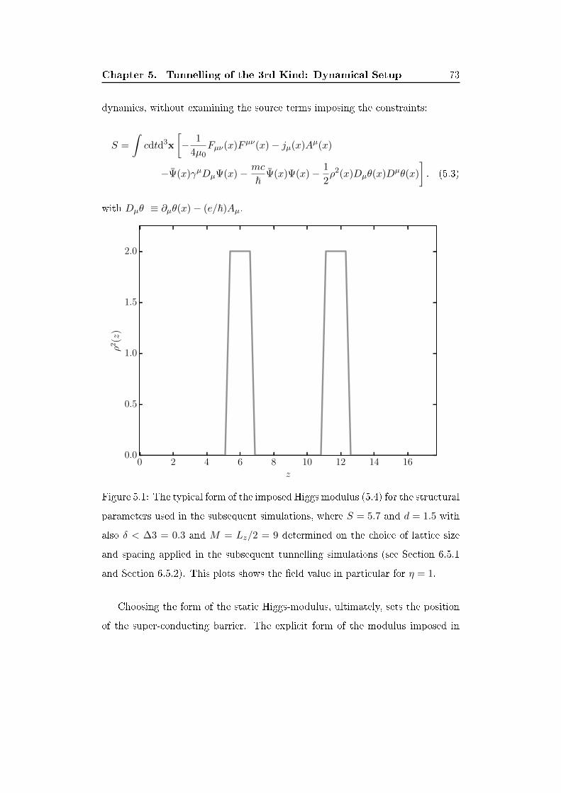
Chapter 5. Tunnelling of the 3rd Kind: Dynamical Setup 73
dynamics, without examining the source terms imposing the constraints:
S =
∫cdtd3x
[− 1
4µ0Fµν(x)Fµν(x)− jµ(x)Aµ(x)
−Ψ(x)γµDµΨ(x)− mc
~Ψ(x)Ψ(x)− 1
2ρ2(x)Dµθ(x)Dµθ(x)
]. (5.3)
with Dµθ ≡ ∂µθ(x)− (e/~)Aµ.
Figure 5.1: The typical form of the imposed Higgs modulus (5.4) for the structural
parameters used in the subsequent simulations, where S = 5.7 and d = 1.5 with
also δ < ∆3 = 0.3 and M = Lz/2 = 9 determined on the choice of lattice size
and spacing applied in the subsequent tunnelling simulations (see Section 6.5.1
and Section 6.5.2). This plots shows the �eld value in particular for η = 1.
Choosing the form of the static Higgs-modulus, ultimately, sets the position
of the super-conducting barrier. The explicit form of the modulus imposed in

Chapter 5. Tunnelling of the 3rd Kind: Dynamical Setup 74
the simulations is
ρ2(x) = ρ2(x3) ≡ 2η2
− η2
[tanh
(x3 + S/2 + d/2−M
δ
)tanh
(x3 + S/2− d/2−M
δ
)
+ tanh
(x3 − S/2 + d/2−M
δ
)tanh
(x3 − S/2− d/2−M
δ
)]. (5.4)
This creates two sheets aligned perpendicular to the z-direction (�gure 5.1).
The sheets are separated a distance S on the z-axis and equidistant from the
coordinate M along this direction. Each barrier extends a �nite width d in
the z-direction and throughout the entire perpendicular plane. The barriers each
increase to a maximum amplitude of ρ2(x3) = 2η2, with the parameter δ de�ning
the skin-width of the tanh function, in increasing from zero to the maximum
barrier strength.
5.1.3 Equations of Motion
Implementing the variational principle on the action (5.3) and choosing the tem-
poral gauge A0 ≡ 0 within the gauge freedom yields the dynamical equations:
1
µ0cΣi∂iEi(x)− i q
~Ψ(x)γ0Ψ(x) +
e
~ρ2(x)D0θ(x)− j0(x) = 0, (5.5a)
1
µ0c∂0Ei(x) +
1
µ0Σj∂jFji(x) + i
q
~Ψ(x)γiΨ(x)
+e
~ρ2(x)Diθ(x)− ji(x) = 0, (5.5b)
(γµDµ +
mc
~
)Ψ(x) = 0, (5.5c)
∂µ(ρ2(x)Dµθ(x)
)= 0, (5.5d)
Chapter 5. Tunnelling of the 3rd Kind: Dynamical Setup 75
with the temporal gauge on the chosen �at-space metric implying
Ei(x) = −c∂0Ai(x); (5.6)
the gauge �eld similarly determines the magnetic �eld through
Ba(x) =∑b,c
εabc∂bAc. (5.7)
These equations comprise the classical dynamics in the unconstrained, 3 + 1
dimensional system without imposing in particular any symmetry assumptions
on the �eld evolution. The electromagnetic �elds thus evolve coupled to the
superconducting barrier and the fermionic interaction, in the presence also of the
external current. Both the fermionic and the Higgs back-reaction onto the gauge
�eld contribute to the evolution in an analogous manner to this external current:
in e�ect, forming respectively a fermionic and Higgs current contribution to the
net current and likewise a fermion and Higgs charge contributing to the total
electric charge.
5.2 Continuum Quantum-Dynamics
5.2.1 Quantized Equations of Motion
The fermions require a quantum analysis to examine these intrinsically-quantum
particles. Contrastingly, the gauge �eld will form a sizeable magnetic �eld (and
ideally no electric �eld); hence, the gauge �eld corresponds to large occupation
numbers and, thus, occupies the classical regime. The Higgs �eld, modelling the
superconducting sheets, represents a classical barrier to a magnetic �eld, and
hence, may also reasonably be assumed to e�ectively occupy the classical regime.
A semi-classical analysis therefore, is employed to examine the system: a classical
treatment determines both the gauge and Higgs �eld dynamics, with the fermions

Chapter 5. Tunnelling of the 3rd Kind: Dynamical Setup 76
in the quantum regime.
Completing this (limited) quantization promotes the fermionic �eld and the
conjugate momentum to an operator in the Heisenberg representation and im-
poses the canonical commutation relations on these operators:
{Ψa(t,x), Ψ†b(t,y)} = ~c (2π)3 δ3(x− y)δab. (5.8)
Applying the Heisenberg equation of motion (2.7) to these �elds, equivalently to
the scalar �eld for the oscillon, yields the quantum dynamics of the fermions.
These, in e�ect, simply convert the �eld in the classical equation (5.5c) to the
corresponding Heisenberg operator. Applying the Heisenberg equations to the
gauge �eld in a complete quantization of the system would, likewise in e�ect,
reproduce the classical equation of motion for the gauge �eld, except converting
the gauge, electric and fermion �elds to operators. The quantum dynamics for the
gauge �eld, where this �eld is to be treated classically, may therefore simply be
obtained on converting the fermion �eld to an operator in the classical dynamics
(5.5a) and (5.5b).
Forming, lastly, the quantum expectation of these gauge-�eld operator equa-
tions yields the semi-quantized dynamics of the system:
1
µ0cΣi∂iEi(x)− i q
~〈T ˆΨ(x)γ0Ψ(x)〉+
e
~ρ2(x)D0θ(x)− j0(x) = 0, (5.9a)
1
µ0c∂0Ei(x) +
1
µ0Σj∂jFji(x) + i
q
~〈T ˆΨ(x)γiΨ(x)〉
+e
~ρ2(x)Diθ(x)− ji(x) = 0, (5.9b)
(γµDµ +
mc
~
)Ψ(x) = 0, (5.9c)
∂µ(ρ2(x)Dµθ(x)
)= 0. (5.9d)
The quantized fermions, thus, evolve under the equation (5.9c) in a background of
Chapter 5. Tunnelling of the 3rd Kind: Dynamical Setup 77
classical electromagnetic �elds and a superconducting barrier. This fermion �eld
back-reacts through the fermionic current in the equation (5.9b), onto the gauge-
�eld evolution. The quantum dynamics notably match the classical dynamics,
except the fermion dynamics now determine the behaviour of the operator �eld
and, most importantly, the gauge equations evolve the quantum, two-point cor-
relators of the fermion �eld. These importantly result on a precise quantum
treatment, in the limit where the gauge and Higgs �eld behave classically; and,
thus, the fermion correlators comprehensively encapsulate the quantum evolution
(both on- and o�-shell) to examine the consequent tunnelling e�ects.
5.2.2 Mode Expansion
An expression of the fermionic-�eld operator in the mode-space may provide the
basis to evaluate the fermion correlators determining the dynamics. The mode
expansion in particular may be constructed to satisfy
Ψ(x) =√~cVx
∑s
∫d3k
(2π)3
(bk,sψ
(U)k,s (x) + d†k,sψ
(V )k,s (x)
), (5.10)
where Vx is the total, real-space volume. Each of {ψ(U)k,s } and {ψ
(V )k,s } comprises an
orthonormal set with these mode functions independently satisfying the fermion
equation of motion (5.5c):
(γµDµ +m)ψ(A)k,s (x) = 0. (5.11)
The {b†k,s} {bk,s} are respectively the creation and annihilation operators
for the fermionic particle and {d†k,s} {dk,s} are respectively the creation and
annihilation operators for the anti-particle. These are time-independent and
Chapter 5. Tunnelling of the 3rd Kind: Dynamical Setup 78
asserted to satisfy1
{bk,s, dl,r} = 0,
{b†k,s, dl,r} = 0;
{bk,s, b†l,r} = V −2x (2π)3 δ3(k− l)δsr,
{dk,s, d†l,r} = V −2
x (2π)3 δ3(k− l)δsr. (5.12)
The annihilation operators conjointly also de�ne the vacuum state:
bk,s |0〉 = 0,
dk,s |0〉 = 0 ∀k, s. (5.13)
This provides a standard, initial state of the system; and in the Heisenberg
picture, remains the state vector acted on at later times.
Substituting therefore the mode expansion (5.10) into the correlators forming
the fermionic currents, applying the de�nition of the vacuum state and also the
1 The choice of the ladder anti-commutators imposes a standard con�guration to satisfy theconstraint for the mode expansion (5.10) to reproduce the canonical �eld-commutator (5.8).Validating the ladder commutator-structure in general may result on specifying the mode
functions at a particular time and enforcing the consistency constraint. The time invarianceof the �eld commutator hence ensures the determined constraint remains valid throughoutthe evolution; and the time invariance of the ladder operators likewise imply the assertedcommutator structure remains unaltered.This procedure may most readily be accomplished in the particular case of the vacuum
mode functions satisfying the imposed boundary conditions on the space. The vacuum modescomprise the initial modes (see also Section 5.6.1), and therefore con�rming the ladder com-mutators reproduce the canonical �eld-commutator for these modes may validate the choice ofthe asserted structure of anti-commutators. The process, also, is expressly demonstrated, sub-sequently, in the non-standard case of the ansatz mode-expansion with Neumann boundarieson the lattice in the Section 5.6.1.The necessary condition on the ladder operators enables further considerable variation in
the potential anti-commutator structures. This choice of the V −2x (2π)3 factors in the relations
implies the dimensionality of the ladder operators equals the inverse square-root of volume;and hence the number operators b†k,sbk,s and d†k,sdk,s corresponding to the ladder operatorsform variables of dimensionality equal to the inverse volume. The eigenvalues of the numberoperators therefore for this choice of the anti-commutators might be associated directly to thenumber density of the fermion particles in the mode k.

Chapter 5. Tunnelling of the 3rd Kind: Dynamical Setup 79
ladder commutators (5.12) yields
〈T ˆΨ(x)γµΨ(x)〉 =~c2
∑s
∫d3k
(2π)3
(ψ
(V )k,s (x)γµψ
(V )k,s (x)− ψ(U)
k,s (x)γµψ(U)k,s (x)
),
(5.14)
with ψ(A)k,s ≡ iψ
(A)†k,s γ
0. This expression of the correlator in the modes, thus
notably incorporates the quantum structure, implicitly, through the application
of the ladder commutators in obtaining the �nal expression.
The correlator expansion substituted into both the electric �eld equations
(5.9b) and (5.9a) and the mode dynamics (5.11), together with the expression
of the electric �eld in the temporal gauge (5.6) and the Higgs dynamics (5.5d),
therefore, fully de�ne the evolution of the quantized system.
5.2.3 The Ensemble Approach
An ensemble of �elds, analogously to the Ensemble Method in the bosonic case
(Section 2.3), may consistently replace the fermionic operator throughout the
gauge-�eld system to determine these semi-quantized dynamics. This method in
the fermionic case involves two sets of �elds to reproduce the correlator structure
of the fermions. These �elds in the respective sets are labelled `male', ΨM,c and
`female', ΨF,c conventionally, where the second index denotes the distinct element
within the set. The male and female �elds respectively are constructed according
to
ΨM,c(x) =
√~c2Vx∑s
∫d3k
(2π)3
(ξk,s,cψ
(U)k,s (x) + ζk,s,cψ
(V )k,s (x)
),
ΨF,c(x) =
√~c2Vx∑s
∫d3k
(2π)3
(ξk,s,cψ
(U)k,s (x)− ζk,s,cψ
(V )k,s (x)
),
where {ψ(U)k,s } and {ψ
(V )k,s } are exactly the previous, fermionic modes with {ξk,s,c}
and {ζk,s,c} each comprising a set of complex, random numbers. A statistical
average 〈·〉E over the ensemble may specify the random numbers and hence �elds
Chapter 5. Tunnelling of the 3rd Kind: Dynamical Setup 80
forming the system.
The two sets of random numbers at each wave-vector are asserted to be inde-
pendent both from one another and likewise from the distributions at a di�erent
wave-vector. Each set further is chosen in the limit of an in�nite ensemble size
to form a Gaussian distribution of mean zero and variance
〈ξk,sξ∗l,r〉E = 〈ζk,sζ∗l,r〉E = V −2x (2π)3 δ3(k− l)δsr,
where the variables in this limit denote a frequency density and, accordingly, the
statistical average involves an integration over the variable space.
This, on applying the de�nition of the vacuum state (5.13) provides direct
equality between the renormalized correlators forming the fermionic current and
the variance of the male and female �elds at a particular instant:
〈T ˆΨ(x)γµΨ(x)〉 = −1
2
(〈ΨM (x)γµΨF (x)〉E + 〈ΨF (x)γµΨM (x)〉E
). (5.15)
In particular, we may choose the set of the real-part Wk,s,c and imaginary-
part Xk,s,c of the ξk,s,c, and likewise the real-part Yk,s,c and imaginary-part Zk,s,c
of the ζk,s,c each form an independent, Gaussian distribution of mean zero and
ensemble-variance1
2V −2x (2π)3 δ3(k− l)δsr,
to generate the Gaussian constraint on the complex random-numbers. These
constraints on the random numbers hence may yield the equivalence of the en-
semble variance to the fermionic correlator and thus an alternative method to
evaluate the fermionic currents at a particular instant.
The ensemble �elds further each comprise a distinct linear-combination of the
modes; and hence the linearity of the mode equation (5.9c) implies the male and
female �elds individually satisfy the mode dynamics. Evolving the ensemble thus
in e�ect evaluates the evolution of every mode function simultaneously according

Chapter 5. Tunnelling of the 3rd Kind: Dynamical Setup 81
to the mode dynamics:
(γµDµ +m) ΨM/F,c(x) = 0. (5.16)
This moreover ensures that if the equality (5.15) holds at any instant, the result
remains valid throughout the subsequent evolution. Establishing this relation
in particular at the initial time therefore determines the evolved ensemble-�elds
yield the quantum correlators at subsequent times. The fermionic correlator,
thus, may be consistently replaced by the ensemble variance in the electric �eld
equations (5.9a) and (5.9b) to incorporate the quantum e�ects within the system.
Equal sample sizes of the random sets in practice may de�ne the ensemble,
and accordingly the statistical properties entail the discrete average over the
NE sample-size. These reduced sets approximate the Gaussian distribution and
hence yield a variance closely approximating the fermionic correlators at any
instant. This �nite set might therefore highly accurately determine the electric
�eld evolution.
These equations formed on constructing the �nite, statistical variances, and
the ensemble-�eld dynamics (5.16) (replacing the equivalent mode function equa-
tion), together with the electric �eld expression in the temporal gauge (5.6) and
the Higgs dynamics (5.5d) thus provide an alternative method to fully determine
the evolution of the quantum system.
5.2.4 An Ansatz for the Fields
The structure of the superconducting sheets, de�ned through the Higgs �eld,
imposes an intrinsic symmetry in the system that may simplify the dynamics.
Orientating both sheets in the x-y plane, with the two uniform and in�nite
in the x-y direction and separated a �nite distance in the z-direction constrains
the variation in the superconductor to solely along the z-axis, while the x and
y directions are physically identical. The Higgs modulus (5.4) representing this

Chapter 5. Tunnelling of the 3rd Kind: Dynamical Setup 82
positioning hence involves purely a z-dependence.
For the electromagnetic �elds, likewise, generated homogeneously over the
x-y plane and with the fermion current evolving from a uniform con�guration
in this background, the symmetries suggest that the gauge and Higgs �eld both
reduce to a 1 + 1D problem:
θ(x) = θ(t, x3), (5.17a)
Ai(x) = Ai(t, x3), (5.17b)
where gauge indices include the spatial components with A0 ≡ 0 already set in
the choice of the temporal gauge.
To achieve this homogeneity in the electromagnetic �elds requires that the
external current generating the electromagnetic �eld also involves only a z-
dependence:
jµ(x) = jµ(t, x3).
The homogeneity of this con�guration over the x-y plane further implies the elec-
tromagnetic �elds can be aligned in a particular direction without any physically
distinct consequences. To orientate the electric �eld along the x-direction, in
the absence of the fermions and the Higgs �eld, would result from aligning the
external current also in this direction:
ji(x) =
j1(t, x3), i = 1
0, i = 2, 3.
(5.18)
This con�guration thus provides the form for the external current satisfying the
symmetry constraints.
The currents of the Higgs-�eld and fermions forming in reaction to the pro-
duced gauge �elds may reasonably be assumed to match the orientation of the
source generating the electromagnetic �elds: the resulting Higgs and fermionic

Chapter 5. Tunnelling of the 3rd Kind: Dynamical Setup 83
currents in the gauge electric �eld dynamics aligning in the direction of the ex-
ternal current. For the currents, thus, orientated entirely along the x-axis, the
resultant magnetic �eld aligns entirely along the y-axis. A consistent choice of
the gauge �elds for this con�guration is obtained in the simple formulation
Ai(x) =
A1(t, x3), i = 1
0, i = 2, 3.
(5.19)
The homogeneity perpendicular to the z-direction might naively indicate that
the fermion modes likewise satisfy an equation of the form:
ψ(A)k,s (x) = ψ
(A)k,s (t, x3).
Considering the inherently quantum nature of the fermions in the vacuum,
though, indicates this simpli�cation is insu�cient. The free fermion-modes
(through e�ectively setting the gauge �eld to zero in the interacting case (5.11))
satisfy
(γµ∂µ +m)ψ(A)k,s (x) = 0.
This system is solved by respectively the standard positive- and negative-energy
con�guration
ψ(+)k,s = eik·xUk,s ,
ψ(−)k,s = e−ik·xVk,s , (5.20)
where Uk,s and Vk,s specify the constant, four-component spinors satisfying the
resultant equations on substituting the respective con�gurations into the vacuum
dynamics. These con�gurations notably incorporate a dependence on each spatial
coordinate even in the entirely isotropic vacuum.
This indicates that any ansatz for the fermion modes must incorporate this
Chapter 5. Tunnelling of the 3rd Kind: Dynamical Setup 84
dependence on every spatial direction; moreover, the assertion (in deriving the
fermionic correlator (5.14)) that the system evolves from the vacuum state im-
plies that the standard result may exactly specify the initial con�guration of the
ansatz in the case where these solutions also satisfy the boundary conditions.
The application of Neumann boundary conditions in the z-direction expectedly
will alter the initial condition2; the separation of the spatial coordinates into
distinct factors in the original solution further indicates that the change to the
boundary conditions in only the z-direction will alter only the factor including
the z-component. Hence, the �elds corresponding respectively to the positive
and negative energy solutions at the initial time may reasonably be asserted to
satisfy
ψ(U)(k1,k2,λ,s)
(0,x) = eik1x1eik2x2χ(U)(k1,k2,λ,s)
(0, x3),
ψ(V )(−k1,−k2,−λ,s)(0,x) = e−ik1x1e−ik2x2χ
(V )(−k1,−k2,−λ,s)(0, x3),
where the variable λ labels each element in a complete and orthonormal set of
�eld-con�gurations3.
2The precise vacuum state for the Neumann boundaries is obtained on the lattice sub-sequently in Section 5.6.1 where the detailed form is explicitly distinct from the standard,continuum expression simply discretized onto the lattice.
3The operator pi = −i~∂i may de�ne the momentum in the ith direction with the eigenvaluescorrespondingly specifying the momentum of the fermion particles in this direction. Acting thisoperator on the fermion vacuum-solutions (5.20), hence, readily determines the values ±~kiform the momentum of the fermion in the ith direction, and the variable ±ki, correspondingly,speci�es the wave-vector in the ith direction.This analysis remains valid in the x1 and x2 directions for the fermion ansatz, and thus the
wavevector k1 and k2 remain the relevant variables labelling these directions. Contrastingly,the χ
(A)
(k1,k2,λ,s)in the ansatz for the fermion modes are not necessarily eigenfunctions of the
momentum operators and, hence, the variable λ may not necessarily correspond to the particlemomentum.The choice of the initial modes in the ansatz, subsequently (Section 5.6.1), incorporate a
linear combination of the standard vacuum solutions. This therefore implies the wave-vector k3
distinguishes the initial modes and thus, forms the particular value of λ, labelling each mode, atthe initial time. The χ
(A)
(k1,k2,λ,s)in the modes though, are each subsequently evolved according
to the coupled, semi-quantized dynamics of the system (5.28). These at later times, therefore,will not necessarily form functions involving a linear combination of the vacuum modes norotherwise necessarily, remain an eigenfunction of the momentum operator. The wave-vector k3
will, therefore, not necessarily remain the relevant variable to label these functions throughoutthe evolution; while the more general variable λ may denote the element in the (complete and

Chapter 5. Tunnelling of the 3rd Kind: Dynamical Setup 85
While the electric and magnetic �elds break the identical state of the x-y di-
rections in the presence only of the superconductor, the fermions interact � rather
than with the physical, electromagnetic �elds � directly with the gauge �eld that,
under the simplifying symmetry assumption, depends only on the z-coordinate
and is homogeneous over the x-y plane. The fermion dynamics thus exclude any
source of potential variation in these directions and hence the initial con�gura-
tion in these dimensions might reasonably remain unaltered in the ansatz at all
times with the time dependence solely in the z-dependent factor. This perma-
nent identicality of the x and the y-directions further consistently matches the
asserted, constant homogeneity of the interactions a�ecting the fermion evolu-
tion. The ansatz for the fermions incorporating the semi-quantum dynamics thus
reasonably imposes
ψ(U)(k1,k2,λ,s)
(x) = eik1x1eik2x2χ(U)(k1,k2,λ,s)
(t, x3),
ψ(V )(−k1,−k2,−λ,s)(x) = e−ik1x1e−ik2x2χ
(V )(−k1,−k2,−λ,s)(t, x3),
where the variable λ label the elements in the complete and orthonormal set of
modes to form the expansion of the fermion �eld.
Substituting this form into the mode expansion (5.10) and accordingly switch-
ing the z-integral to vary over the ansatz-label λ in the modi�ed direction4 there-
fore yields the expansion in the mode ansatz; with the ladder operators likewise
relabelled to denote association to this alternative variable:
Ψ(x) =√~cVx
∑s
∫dk1
(2π)
dk2
(2π)
dλ
(2π)
[b(k1,k2,λ,s)e
ik1x1eik2x2χ(U)(k1,k2,λ,s)
(t, x3)
+ d†(k1,k2,λ,s)e−ik1x1e−ik2x2χ
(V )(−k1,−k2,−λ,s)(t, x3)
].
orthonormal) set of �eld con�gurations throughout the evolution.4The explicit form of the integration-weighting dλ/(2π) might be determined through the
relation of the mode functions to the fermionic anti-commutator � equivalently to the discreteanalogue ∆λ/(2π) (see Section 5.6.1).

Chapter 5. Tunnelling of the 3rd Kind: Dynamical Setup 86
The ladder-operator anti-commutators correspondingly are asserted to satisfy
{b(k1,k2,λ,s), d(l1,l2,υ,r)} = 0,
{b†(k1,k2,λ,s), d(l1,l2,υ,r)} = 0;
{b(k1,k2,λ,s), b†(l1,l2,υ,r)
} = V −2x (2π)3 δ(k1 − l1)δ(k2 − l2)δ(λ− υ)δsr,
{d(k1,k2,λ,s), d†(l1,l2,υ,r)
} = V −2x (2π)3 δ(k1 − l1)δ(k2 − l2)δ(λ− υ)δsr, (5.21)
where notably, the ansatz-label λ replaces the wave-vector in the delta function
compared to the operator relations (5.12) in the standard expansion5.
Implementing the transformation k1,2 → −k1,2, λ→ −λ on the second term
of the ansatz expansion yields the expression
Ψ(x) =√~cVx
∑s
∫dk1
(2π)
dk2
(2π)
dλ
(2π)
[b(k1,k2,λ,s)e
ik1x1eik2x2χ(U)(k1,k2,λ,s)
(t, x3)
+ d†(−k1,−k2,−λ,s)eik1x1eik2x2χ
(V )(k1,k2,λ,s)
(t, x3)];
(5.22)
both the positive- and the negative-energy ansatz in the expansion thereby reduce
to the identical, general form
ψ(A)(k1,k2,λ,s)
(x) = eik1x1eik2x2χ(A)(k1,k2,λ,s)
(t, x3),
thus simplifying the fermion ansatz.
This form for the fermion modes together with the selected, spatial gauge-
con�guration (5.19) and the Higgs phase (5.17a) provide the ansatz for the �eld
evolution under the choice of the temporal gauge, in the presence of the speci�ed
5The structure of the ladder anti-commutators may ultimately be validated through theiruse to generate the �eld commutator (5.8), equivalently to the ladder commutators in the modefunction case (see footnote 1).This procedure will be demonstrated subsequently in the ansatz-case on the lattice with
Neumann boundaries (Section 5.6.1).

Chapter 5. Tunnelling of the 3rd Kind: Dynamical Setup 87
external current (5.18) and the chosen structure of the Higgs modulus (5.4).
Substituting the gauge and Higgs-phase ansatz into the electric �eld evolution
(5.9a) and (5.9b) and the Higgs dynamics (5.9d) with the modulus structure (5.4)
and imposed external-current (5.18) yields
iq
~〈T ˆΨ(x)γ0Ψ(x)〉 − e
~ρ2(x3)∂0θ(t, x3) + j0(t, x3) = 0, (5.23)
iq
~〈T ˆΨ(x)γ2,3Ψ(x)〉+
e
~ρ2(x3)∂0θ(t, x3) = 0, (5.24)
1
µ0c∂0E1(t, x3) +
1
µ0∂2
3A1(t, x3) + iq
~〈T ˆΨ(x)γ1Ψ(x)〉
−( e~
)2ρ2(x3)A1(t, x3)− j1(t, x3) = 0, (5.25)
(ρ2(x3)
[∂2
0 − ∂23
]− 2ρ(x3)∂3ρ(x3)∂3
)θ(t, x3) = 0; (5.26)
where
E1(t, x3) = −c∂0A1(t, x3) (5.27)
results on applying the gauge ansatz to the electric �eld expression (5.6). Like-
wise, the gauge, Higgs-phase and mode ansatz substituted into the mode function
dynamics (5.11) with the modulus structure (5.4) determines
(γ0∂0 + i
[k1 − i
q
~A1(t, x3)
]γ1 + ik2γ
2 + γ3∂3 +mc
~
)χ
(A)(k1,k2,λ,s)
(t, x3) = 0.
(5.28)
Substituting the ansatz-expansion (5.22) also into the fermionic-correlator, on
applying the ladder anti-commutator (5.21) and vacuum-state de�nition (5.13)

Chapter 5. Tunnelling of the 3rd Kind: Dynamical Setup 88
yields
〈T ˆΨ(x)γµΨ(x)〉 =
~c2
∑s
∫dk1
(2π)
dk2
(2π)
dλ
(2π)
(χ
(V )(k1,k2,λ,s)
(t, x3)γµχ(V )(k1,k2,λ,s)
(t, x3)
− χ(U)(k1,k2,λ,s)
(t, x3)γµχ(U)(k1,k2,λ,s)
(t, x3)), (5.29)
with χ(A)(k1,k2,λ,s)
≡ iχ(A)†(k1,k2,λ,s)
γ0. This expansion in the mode ansatz (equivalently
to the standard mode expansion, Section 5.2.2), thus, implicitly incorporates the
quantum structure through the application of the ladder commutators. These
results for the ansatz, importantly therefore, simplify the quantum dynamics to
a one-dimensional system varying only over the z-direction in coordinate space,
with the correlator involving a summation over a three-dimensional mode-space.
The Higgs-�eld phase entirely decouples from the gauge and fermionic �elds,
and thus has no e�ect on the electromagnetic �elds interacting with the barrier,
with or without fermions present. Hence, we may for simplicity neglect the phase
throughout the evolution � in e�ect choosing θ(t, x3) = 0 to satisfy the evolution
equation (5.5d) � without constraint on the interactions of principal interest.
This assertion therefore eliminates the phase evolution from the dynamics;
and further determines the gauge constraints (5.23) and (5.24) in the ansatz
satisfy
iq
~〈T ˆΨ(x)γ0Ψ(x)〉+ j0(t, x3) = 0,
iq
~〈T ˆΨ(x)γ2Ψ(x)〉 = 0,
iq
~〈T ˆΨ(x)γ3Ψ(x)〉 = 0.
These results thus specify the constraints on the gauge �eld in the ansatz case;
while the electric �eld dynamics (5.25) and mode function ansatz-equation (5.28),
together with the corresponding correlator expansion (5.29) and the expression of
Chapter 5. Tunnelling of the 3rd Kind: Dynamical Setup 89
the electric �eld (5.27) in the ansatz may fully determine the quantized evolution
under the inherent symmetries of the system.
5.3 Tunnelling of the 3rd Kind: Simple Estimate
An e�ective one-loop action provides the basis in perturbative expressions ob-
tained for tunnelling of the 3rd kind (see [98] for details). These calculations
in a comparable system to the present con�guration but involving only a single
barrier imply the constant, external �eld Bext induces a �eld Bint having crossed
the barrier through the tunnelling process. The transmission asymptotically far
from the barrier results proportionately to the external �eld, in the ratio
|Bint||Bext|
=q2
48π2
∫ ∞1
dτ
τ4
√τ2 − 1
(1 + 2τ2
)exp(−2mdτ), (5.30)
for the fermion mass m and charge q through the barrier of thickness d, with
the result obtained in natural units � matching, importantly, the analysis in the
subsequent tunnelling simulations. This integral is to be evaluated analytically,
and for m = 1, q = 0.3, e = 1 and d = 1.5, chosen in the ensuing simulations
(Section 6.1 and 6.5.1), hence yields |Bint|/|Bext| = 3.4 · 10−6. The present
con�guration in contrast to the analytic case involves two barriers and encloses
the tunnelled �eld within a �nite distance from the barriers. This therefore
indicates the true result in the simulated case involves a multiplicative correction
between one and two to the analytic estimate.
A superconducting barrier experimentally would induce the distinctive ex-
ponential decay in the magnetic �eld; and the Higgs-�eld model likewise can
reproduce this characteristic decay. Solving the continuum dynamics exclud-
ing the fermions can, therefore, provide an estimate for the classical �eld decay
through the barrier. Adding this to the tunnelling result hence forms a rea-
sonable estimate for the observed transmission. The classical solution further
enables distinguishing the contrastive tunnelling e�ects.

Chapter 5. Tunnelling of the 3rd Kind: Dynamical Setup 90
Establishing the constant magnetic �eld outside the superconducting enclo-
sure essentially produces a static, �nal state for measuring the transmission.
Accordingly setting the gauge �elds constant in the electric �eld dynamics (5.25)
(incorporating the symmetries) outside the external current and for the fermions
omitted hence implies
∂23A1(t, x3) = −e2ρ2(x3)A1,
on also imposing natural units to match the tunnelling case � and the subsequent
simulations. A step-function of the maximum barrier amplitude 2η2 provides an
accurate and simple approximation to the barrier con�guration in the limiting
case where the modulus function rises steeply � on setting δ su�ciently small.
This provides a readily tractable system; the classical solutions in this case simply
satisfy
A1(t, x3) = A1,ext exp(−√
2eη),
where imposing continuity at the exterior boundary to the barrier further de-
termines A1,ext equals the gauge �eld adjoining this boundary. The gauge-�eld
relation to the magnetic �eld (5.7) hence readily determines the magnetic �eld
B2,int inside the enclosure satis�es
B2,int(t, x3) = B2,ext exp(−√
2eη), (5.31)
where again the continuity at the boundary implies B2,ext, equals the (uniform)
external value. This accordingly provides the estimate to add to the tunnelling
contribution and for contrasting the classical and quantum cases.
The �gure 5.2 shows the constant tunnelling contribution and the varying
transmission on changing the wall thickness for e = 1 and d = 1.5 in the case
without fermions and, additionally, q = 0.3 and m = 1 with the fermions �
notably, matching the parameter choice in the subsequent simulations. The tun-
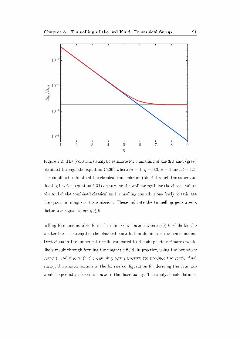
Chapter 5. Tunnelling of the 3rd Kind: Dynamical Setup 91
Figure 5.2: The (constant) analytic estimate for tunnelling of the 3rd kind (grey)
obtained through the equation (5.30) where m = 1, q = 0.3, e = 1 and d = 1.5;
the simpli�ed estimate of the classical transmission (blue) through the supercon-
ducting barrier (equation 5.31) on varying the wall strength for the chosen values
of e and d; the combined classical and tunnelling contributions (red) to estimate
the quantum magnetic-transmission. These indicate the tunnelling generates a
distinctive signal where η & 6.
nelling fermions notably form the main contribution where η & 6 while for the
weaker barrier strengths, the classical contribution dominates the transmission.
Deviations in the numerical results compared to the simplistic estimates would
likely result through forming the magnetic �eld, in practice, using the boundary
current, and also with the damping terms present (to produce the static, �nal
state); the approximation to the barrier con�guration for deriving the estimate
would expectedly also contribute to the discrepancy. The analytic calculations,

Chapter 5. Tunnelling of the 3rd Kind: Dynamical Setup 92
though, usefully indicate the approximate tunnelling contribution. This hence
will enable evaluating whether the perturbative (one-loop) approximations for
the tunnelling accurately describe the resultant signal. These estimates more-
over indicate the regime where the signal deviates from the classical case; and
thus, usefully, indicates the barrier strengths to examine for detecting this tun-
nelling signal.
5.4 Discretized Dynamics
5.4.1 Action
We discretize the system onto a lattice through the action while retaining the
U(1) symmetry (5.1) through the application of a link-function to incorporate
both the gauge �elds and the Higgs phase:
S(X) =
1
c∆V
[∑i
~2
2qµ0(∆xi)2(∆x0)2(2− Ui0(X)− U0i(X))
−∑ij
~2
4q2µ0(∆xi)2(∆xj)2(2− Uij(X)− Uji(X))
−∑µ
1
2∆xµΨ(X)γµ
(Uµ(X)Ψ(X + µ)− U †µ(X − µ)Ψ(X − µ)
)+mc
~Ψ(X)Ψ(X)
+ρ2(X)
2(∆x0)2
(2−Θ†(X)U
e/q0 (X)Θ(X + 0)−Θ†(X + 0)U
(e/q)†0 (X)Θ(X)
)−∑i
ρ2(X)
2(∆xi)2
(2−Θ†(X)U
e/qi (X)Θ(X + i)−Θ†(X + i)U
(e/q)†i (X)Θ(X)
)],
(5.32)
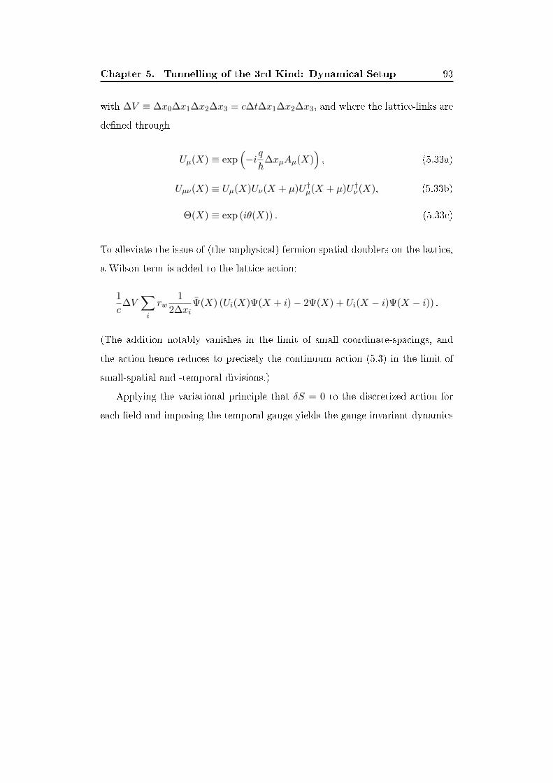
Chapter 5. Tunnelling of the 3rd Kind: Dynamical Setup 93
with ∆V ≡ ∆x0∆x1∆x2∆x3 = c∆t∆x1∆x2∆x3, and where the lattice-links are
de�ned through
Uµ(X) ≡ exp(−i q
~∆xµAµ(X)
), (5.33a)
Uµν(X) ≡ Uµ(X)Uν(X + µ)U †µ(X + µ)U †ν (X), (5.33b)
Θ(X) ≡ exp (iθ(X)) . (5.33c)
To alleviate the issue of (the unphysical) fermion spatial-doublers on the lattice,
a Wilson term is added to the lattice action:
1
c∆V
∑i
rw1
2∆xiΨ(X) (Ui(X)Ψ(X + i)− 2Ψ(X) + Ui(X − i)Ψ(X − i)) .
(The addition notably vanishes in the limit of small coordinate-spacings, and
the action hence reduces to precisely the continuum action (5.3) in the limit of
small-spatial and -temporal divisions.)
Applying the variational principle that δS = 0 to the discretized action for
each �eld and imposing the temporal gauge yields the gauge-invariant dynamics
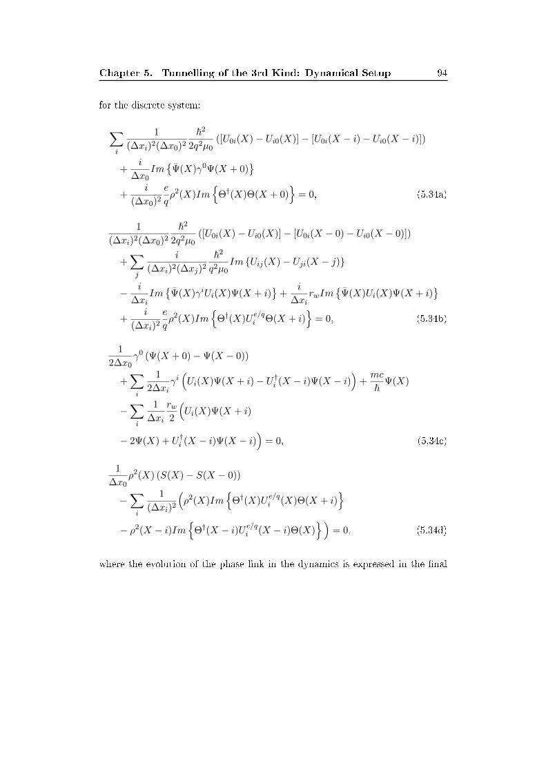
Chapter 5. Tunnelling of the 3rd Kind: Dynamical Setup 94
for the discrete system:
∑i
1
(∆xi)2(∆x0)2
~2
2q2µ0([U0i(X)− Ui0(X)]− [U0i(X − i)− Ui0(X − i)])
+i
∆x0Im{
Ψ(X)γ0Ψ(X + 0)}
+i
(∆x0)2
e
qρ2(X)Im
{Θ†(X)Θ(X + 0)
}= 0, (5.34a)
1
(∆xi)2(∆x0)2
~2
2q2µ0([U0i(X)− Ui0(X)]− [U0i(X − 0)− Ui0(X − 0)])
+∑j
i
(∆xi)2(∆xj)2
~2
q2µ0Im {Uij(X)− Uji(X − j)}
− i
∆xiIm{
Ψ(X)γiUi(X)Ψ(X + i)}
+i
∆xirwIm
{Ψ(X)Ui(X)Ψ(X + i)
}+
i
(∆xi)2
e
qρ2(X)Im
{Θ†(X)U
e/qi Θ(X + i)
}= 0, (5.34b)
1
2∆x0γ0 (Ψ(X + 0)−Ψ(X − 0))
+∑i
1
2∆xiγi(Ui(X)Ψ(X + i)− U †i (X − i)Ψ(X − i)
)+mc
~Ψ(X)
−∑i
1
∆xi
rw2
(Ui(X)Ψ(X + i)
− 2Ψ(X) + U †i (X − i)Ψ(X − i))
= 0, (5.34c)
1
∆x0ρ2(X) (S(X)− S(X − 0))
−∑i
1
(∆xi)2
(ρ2(X)Im
{Θ†(X)U
e/qi (X)Θ(X + i)
}− ρ2(X − i)Im
{Θ†(X − i)U e/qi (X − i)Θ(X)
})= 0, (5.34d)
where the evolution of the phase link in the dynamics is expressed in the �nal
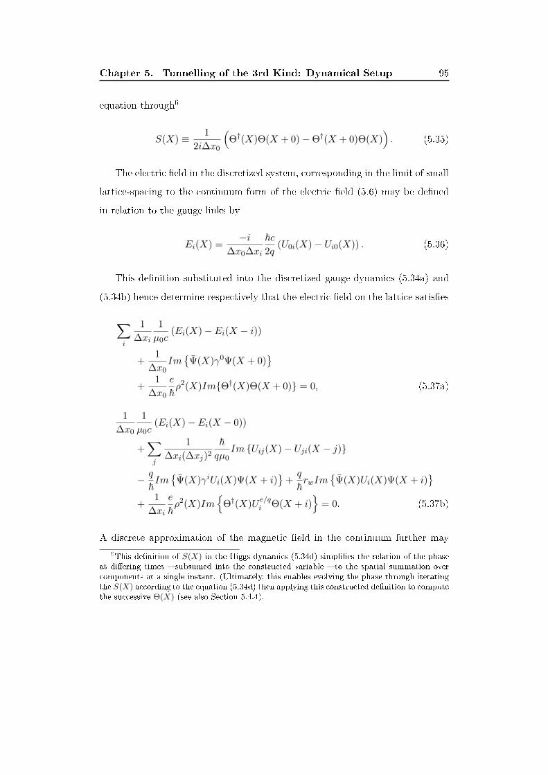
Chapter 5. Tunnelling of the 3rd Kind: Dynamical Setup 95
equation through6
S(X) ≡ 1
2i∆x0
(Θ†(X)Θ(X + 0)−Θ†(X + 0)Θ(X)
). (5.35)
The electric �eld in the discretized system, corresponding in the limit of small
lattice-spacing to the continuum form of the electric �eld (5.6) may be de�ned
in relation to the gauge links by
Ei(X) =−i
∆x0∆xi
~c2q
(U0i(X)− Ui0(X)) . (5.36)
This de�nition substituted into the discretized gauge-dynamics (5.34a) and
(5.34b) hence determine respectively that the electric �eld on the lattice satis�es
∑i
1
∆xi
1
µ0c(Ei(X)− Ei(X − i))
+1
∆x0Im{
Ψ(X)γ0Ψ(X + 0)}
+1
∆x0
e
~ρ2(X)Im{Θ†(X)Θ(X + 0)} = 0, (5.37a)
1
∆x0
1
µ0c(Ei(X)− Ei(X − 0))
+∑j
1
∆xi(∆xj)2
~qµ0
Im {Uij(X)− Uji(X − j)}
− q
~Im{
Ψ(X)γiUi(X)Ψ(X + i)}
+q
~rwIm
{Ψ(X)Ui(X)Ψ(X + i)
}+
1
∆xi
e
~ρ2(X)Im
{Θ†(X)U
e/qi Θ(X + i)
}= 0. (5.37b)
A discrete approximation of the magnetic �eld in the continuum further may
6This de�nition of S(X) in the Higgs dynamics (5.34d) simpli�es the relation of the phaseat di�ering times � subsumed into the constructed variable � to the spatial summation overcomponents at a single instant. (Ultimately, this enables evolving the phase through iteratingthe S(X) according to the equation (5.34d) then applying this constructed de�nition to computethe successive Θ(X) (see also Section 5.4.4).
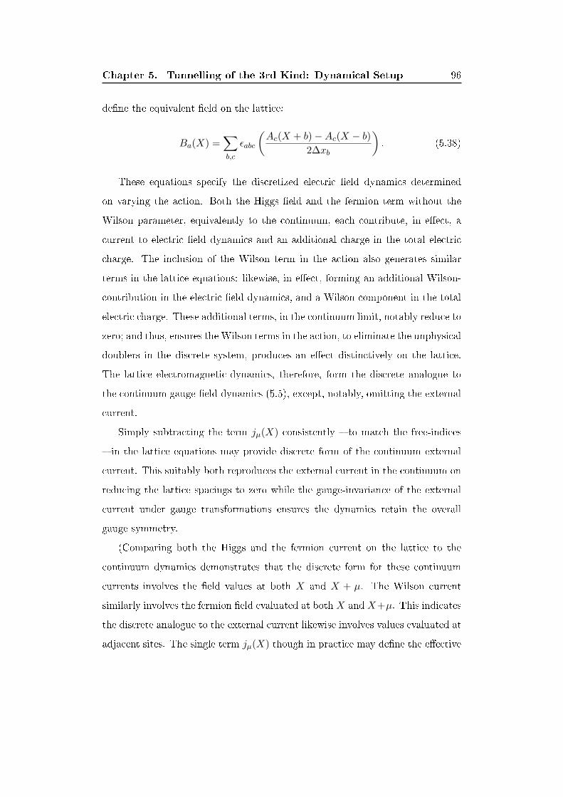
Chapter 5. Tunnelling of the 3rd Kind: Dynamical Setup 96
de�ne the equivalent �eld on the lattice:
Ba(X) =∑b,c
εabc
(Ac(X + b)−Ac(X − b)
2∆xb
). (5.38)
These equations specify the discretized electric �eld dynamics determined
on varying the action. Both the Higgs �eld and the fermion term without the
Wilson parameter, equivalently to the continuum, each contribute, in e�ect, a
current to electric �eld dynamics and an additional charge in the total electric
charge. The inclusion of the Wilson term in the action also generates similar
terms in the lattice equations: likewise, in e�ect, forming an additional Wilson-
contribution in the electric �eld dynamics, and a Wilson component in the total
electric charge. These additional terms, in the continuum limit, notably reduce to
zero; and thus, ensures the Wilson terms in the action, to eliminate the unphysical
doublers in the discrete system, produces an e�ect distinctively on the lattice.
The lattice electromagnetic-dynamics, therefore, form the discrete analogue to
the continuum gauge-�eld dynamics (5.5), except, notably, omitting the external
current.
Simply subtracting the term jµ(X) consistently � to match the free-indices
� in the lattice equations may provide discrete form of the continuum external
current. This suitably both reproduces the external current in the continuum on
reducing the lattice spacings to zero while the gauge-invariance of the external
current under gauge transformations ensures the dynamics retain the overall
gauge symmetry.
(Comparing both the Higgs and the fermion current on the lattice to the
continuum dynamics demonstrates that the discrete form for these continuum
currents involves the �eld values at both X and X + µ. The Wilson current
similarly involves the fermion �eld evaluated at both X and X+µ. This indicates
the discrete analogue to the external current likewise involves values evaluated at
adjacent sites. The single term jµ(X) though in practice may de�ne the e�ective
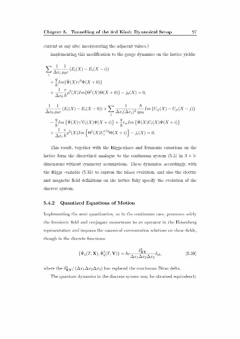
Chapter 5. Tunnelling of the 3rd Kind: Dynamical Setup 97
current at any site: incorporating the adjacent values.)
Implementing this modi�cation to the gauge dynamics on the lattice yields:
∑i
1
∆xi
1
µ0c(Ei(X)− Ei(X − i))
+q
~Im{Ψ(X)γ0Ψ(X + 0)}
+1
∆x0
e
~ρ2(X)Im{Θ†(X)Θ(X + 0)} − j0(X) = 0,
1
∆x0
1
µ0c(Ei(X)− Ei(X − 0)) +
∑j
1
∆xi(∆xj)2
~qµ0
Im {Uij(X)− Uji(X − j)}
− q
~Im{
Ψ(X)γiUi(X)Ψ(X + i)}
+q
~rwIm
{Ψ(X)Ui(X)Ψ(X + i)
}+
1
∆xi
e
~ρ2(X)Im
{Θ†(X)U
e/qi Θ(X + i)
}− ji(X) = 0.
This result, together with the Higgs-phase and fermionic equations on the
lattice form the discretized analogue to the continuum system (5.5) in 3 + 1-
dimensions without symmetry assumptions. These dynamics, accordingly, with
the Higgs -variable (5.35) to express the phase evolution, and also the electric
and magnetic �eld de�nitions on the lattice fully specify the evolution of the
discrete system.
5.4.2 Quantized Equations of Motion
Implementing the semi-quantization, as in the continuum case, promotes solely
the fermionic �eld and conjugate momentum to an operator in the Heisenberg
representation and imposes the canonical commutation relations on these �elds,
though in the discrete functions:
{Ψa(T,X), Ψ†b(T,Y)} = ~cδ3XY
∆x1∆x2∆x3δab, (5.39)
where the δ3XY/ (∆x1∆x2∆x3) has replaced the continuum Dirac-delta.
The quantum dynamics in the discrete system may be obtained equivalently
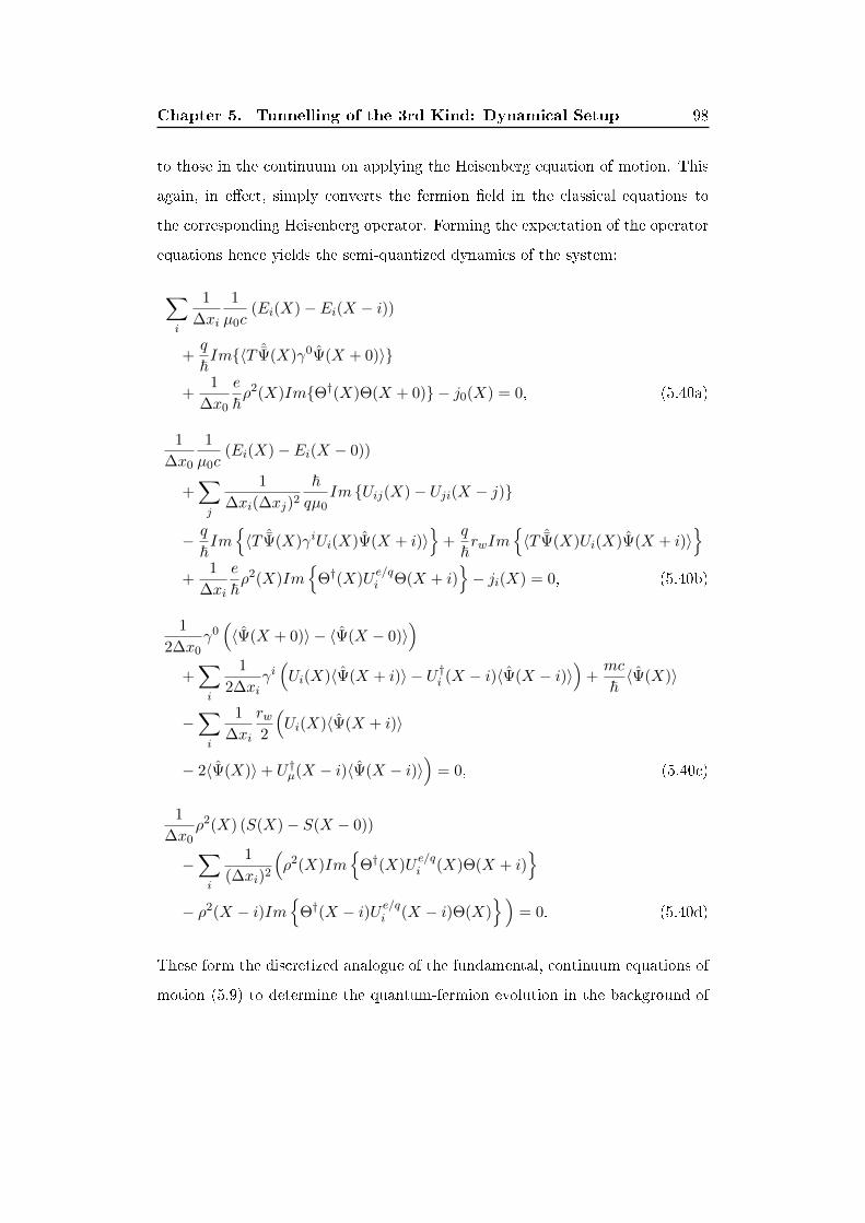
Chapter 5. Tunnelling of the 3rd Kind: Dynamical Setup 98
to those in the continuum on applying the Heisenberg equation of motion. This
again, in e�ect, simply converts the fermion �eld in the classical equations to
the corresponding Heisenberg operator. Forming the expectation of the operator
equations hence yields the semi-quantized dynamics of the system:
∑i
1
∆xi
1
µ0c(Ei(X)− Ei(X − i))
+q
~Im{〈T ˆΨ(X)γ0Ψ(X + 0)〉}
+1
∆x0
e
~ρ2(X)Im{Θ†(X)Θ(X + 0)} − j0(X) = 0, (5.40a)
1
∆x0
1
µ0c(Ei(X)− Ei(X − 0))
+∑j
1
∆xi(∆xj)2
~qµ0
Im {Uij(X)− Uji(X − j)}
− q
~Im{〈T ˆΨ(X)γiUi(X)Ψ(X + i)〉
}+q
~rwIm
{〈T ˆΨ(X)Ui(X)Ψ(X + i)〉
}+
1
∆xi
e
~ρ2(X)Im
{Θ†(X)U
e/qi Θ(X + i)
}− ji(X) = 0, (5.40b)
1
2∆x0γ0(〈Ψ(X + 0)〉 − 〈Ψ(X − 0)〉
)+∑i
1
2∆xiγi(Ui(X)〈Ψ(X + i)〉 − U †i (X − i)〈Ψ(X − i)〉
)+mc
~〈Ψ(X)〉
−∑i
1
∆xi
rw2
(Ui(X)〈Ψ(X + i)〉
− 2〈Ψ(X)〉+ U †µ(X − i)〈Ψ(X − i)〉)
= 0, (5.40c)
1
∆x0ρ2(X) (S(X)− S(X − 0))
−∑i
1
(∆xi)2
(ρ2(X)Im
{Θ†(X)U
e/qi (X)Θ(X + i)
}− ρ2(X − i)Im
{Θ†(X − i)U e/qi (X − i)Θ(X)
})= 0. (5.40d)
These form the discretized analogue of the fundamental, continuum equations of
motion (5.9) to determine the quantum-fermion evolution in the background of
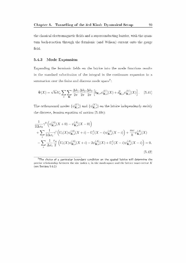
Chapter 5. Tunnelling of the 3rd Kind: Dynamical Setup 99
the classical electromagnetic �elds and a superconducting barrier, with the quan-
tum back-reaction through the fermionic (and Wilson) current onto the gauge
�eld.
5.4.3 Mode Expansion
Expanding the fermionic �elds on the lattice into the mode functions results
in the standard substitution of the integral in the continuum expansion to a
summation over the �nite and discrete mode-space7:
Ψ(X) =√~cVx
∑s
∑K
∆k1
2π
∆k2
2π
∆k3
2π
[bK,sψ
(U)K,s(X) + d†K,sψ
(V )K,s(X)
]. (5.41)
The orthonormal modes {ψ(U)K,s} and {ψ
(V )K,s} on the lattice independently satisfy
the discrete, fermion equation of motion (5.40c):
1
2∆x0γ0(ψ
(A)K,s(X + 0)− ψ(A)
K,s(X − 0))
+∑i
1
2∆xiγi(Ui(X)ψ
(A)K,s(X + i)− U †i (X − i)ψ(A)
K,s(X − i))
+mc
~ψ
(A)K,s(X)
−∑i
1
∆xi
rw2
(Ui(X)ψ
(A)K,s(X + i)− 2ψ
(A)K,s(X) + U †i (X − i)ψ(A)
K,s(X − i))
= 0.
(5.42)
7The choice of a particular boundary condition on the spatial lattice will determine theprecise relationship between the site index ei in the mode-space and the lattice wave-vector K(see Section 5.6.1)

Chapter 5. Tunnelling of the 3rd Kind: Dynamical Setup 100
Asserting, further, the creation and annihilation operators satisfy analogous re-
lations to those in the continuum thus imposes
{bK,s, dL,r} = 0, (5.43a)
{b†K,s, dL,r} = 0; (5.43b)
{bK,s, b†L,r} = V −2
x (2π)3 δsrδ3KL
∆k1∆k2∆k3, (5.43c)
{dK,s, d†L,r} = V −2
x (2π)3 δsrδ3KL
∆k1∆k2∆k3, (5.43d)
where the Dirac delta-function in the respective, continuum commutators has
been substituted for the equivalent Kronecker-delta factor8.
Substituting the discretized mode-expansion (5.41) into the fermionic corre-
8The choice of the ladder anti-commutators ensure the mode-expansion (5.41) satis�es thenecessary constraint to reproduce the canonical �eld-commutator (5.39): equivalently to themode function method in the continuum (see footnote 1).This procedure will be demonstrated subsequently on the lattice, in the non-standard case
of the ansatz mode-expansion with Neumann boundaries (Section 5.6.1).The choice of the V −2
x (2π)3 factor analogous to the continuum case further implies thedimensionality of the ladder operators and hence the corresponding number operators b†K,sbK,s
and d†K,sdK,s in the discrete case likewise match. Hence the eigenvalues of the number operatorsfor the choice of discretized anti-commutators might be be associated directly to the numberdensity of the fermion particles in a mode K on the lattice.An alternative choice in the variety of potential anti-commutators might be to entirely elim-
inate all except the dimensionless factors in the relations; and accordingly modify the factorsin the mode-expansion to satisfy the condition to reproduce the canonical �eld-commutator.This con�guration implies the ladder operators and hence corresponding number operators toequally be dimensionless. The eigenvalues of the number operators in this system may there-fore be associated directly to the total fermion particle number in the associated mode. Thismay be considered to provide a more sensible quantity on the lattice; with the correspondinganti-commutator structure, accordingly, forming a more sensible choice on the lattice than thedirect equivalence to the continuum.Since the ladder operators occur only in the fermion correlators within the dynamics and these
are invariant under the change in ladder-commutator structure; and further since this studyomits any direct measurement of the particle number, the particular choice of the ladder com-mutator structure is irrelevant to the analysis. The construction of the ladder anti-commutatorson the lattice directly equivalent to the continuum provides a simple uniformity in the choiceof commutator structure.

Chapter 5. Tunnelling of the 3rd Kind: Dynamical Setup 101
lators on the lattice and applying the vacuum-state de�nition (5.13) provides
〈T ˆΨ(X)OΨ(X + µ)〉 =
~c2
∑s
∑K
∆k1
2π
∆k2
2π
∆k3
2π
[ψ
(V )K,s(X)Oψ
(V )K,s(X + µ)
− ψ(U)K,s(X)Oψ
(U)K,s(X + µ)
], (5.44)
for the relevant operators O and direction µ in the dynamics: thus obtaining the
fermion self-interaction on the lattice entirely in terms of the mode functions.
This mode function expression of the correlators (5.40b) and the evolution
(5.42) of the discrete modes together with the de�nition of the electric �eld (5.36)
in terms of the gauge link, and the discretized, classical, Higgs dynamics (5.34d)
may fully de�ne the evolution of the quantized system on the lattice.

Chapter 5. Tunnelling of the 3rd Kind: Dynamical Setup 102
5.4.4 Numerical Evolution: Mode Functions
Rearranging the evolution equations of the electric �eld (5.40b), fermion modes
(5.42) and the Higgs phase (5.40d) provides iteration relations for evolving the
system:
Ei(X) = Ei(X − 0)−∑j
∆x0
∆xi(∆xj)2
~cqIm {Uij(X)− Uji(X − j)}
+ ∆x0µ0cq
~Im{〈T ˆΨ(X)γiUi(X)Ψ(X + i)〉
}−∆x0
µ0cq
~rwIm
{〈T ˆΨ(X)Ui(X)Ψ(X + i)〉
}− ∆x0
∆xi
µ0ce
~ρ2(X)Im
{Θ†(X)U
e/qi Θ(X + i)
}+ ∆x0µ0cji(X), (5.45a)
ψ(A)K,s(X + 0) = ψ
(A)K,s(X − 0)
+∑i
∆x0
∆xiγ0γi
(Ui(X)ψ
(A)K,s(X + i)− U †i (X − i)ψ(A)
K,s(X − i))
+mc
~ψ
(A)K,s(X)
−∑i
∆x0
∆xirwγ
0(Ui(X)ψ
(A)K,s(X + i)
− 2ψ(A)K,s(X) + U †i (X − i)ψ(A)
K,s(X − i)), (5.45b)
S(X) = S(X − 0) +∑i
∆x0
(∆xi)2
(Im{
Θ†(X)Ue/qi (X)Θ(X + i)
}− ρ2(X − i)
ρ2(X)Im{
Θ†(X − i)U e/qi (X − i)Θ(X)})
, (5.45c)
where the expansion (5.44) in the modes on renormalization provides the stan-
dard method to determine the correlators. This evolution further entails deter-
mining both the gauge and phase links. These may be obtained respectively
through the de�nition on the lattice of the electric �eld (5.36) and the variable
S(X) (5.35) expressing the Higgs evolution.
The electric �eld de�nition in the temporal gauge implies
Im{Ui(X + 0)U †i (X)
}= ∆x0∆x1
q
~cEi(X);

Chapter 5. Tunnelling of the 3rd Kind: Dynamical Setup 103
the unitarity of the gauge links, in general, hence yields
Re{Ui(X + 0)U †i (X)
}= ±
√(1−
(∆x0∆xi
q
~cEi(X)
)2),
while the unitarity, in particular, where Ei = 0 consequently determines
Re{Ui(X + 0)U †i (X)
}= +
√(1−
(∆x0∆xi
q
~cEi(X)
)2).
This result on rearrangement therefore provides the iteration relation to evolve
the gauge-link terms in the dynamics:
Ui(X + 0) =
(+
√(1−
(∆x0∆xi
q
~cEi(X)
)2)
+ i∆x0∆x1q
~cEi(X)
)Ui(X).
(5.46)
Likewise, the constructed Higgs-variable S(X) implies
Im{
Θ†(X)Θ(X + 0)}
= ∆x0S(X),
while the unitarity of phase-link in general and at S(X) = 0, together, determine
Re{
Θ†(X)Θ(X + 0)}
= +
√(1− (∆x0S(X))2
);
and hence, the constructed variable S(X) yields the iteration relation to evolve
phase link:
Θ(X + 0) =
(+
√(1− (∆x0S(X))2
)+ i∆x0S(X)
)Θ(X). (5.47)
This expression, the equivalent gauge-link evolution (5.46), and the �eld iter-
ation relations (5.45) with the mode function expansion (5.44) of the correlators
fully specify the dynamics to evolve the system numerically from a given initial
state.

Chapter 5. Tunnelling of the 3rd Kind: Dynamical Setup 104
Con�rming the constraint (5.40a) on the lattice to machine-level accuracy in
addition o�ers a convenient indicator for validating the reliability of the mode
function simulation.
5.4.5 The Ensemble Approach
A summation over the discrete lattice, mode-space replaces the integral over this
space in the continuum, to de�ne the discretized ΨM,c and ΨF,c �elds:
ΨM,c(x) =
√~c2Vx∑s
∑K
∆k1
2π
∆k2
2π
∆k3
2π
1
2ωK
[ξK,s,cψ
(U)K,s(X) + ζK,s,cψ
(V )K,s(X)
],
ΨF,c(x) =
√~c2Vx∑s
∑K
∆k1
2π
∆k2
2π
∆k3
2π
1
2ωK
[ξK,s,cψ
(U)K,s(X)− ζK,s,cψ
(V )K,s(X)
],
and each evolves according to the discretized, fermionic equation of motion
(5.40c).
The independence constraints on the two sets of random numbers at each
wave-vector value are imposed to be identical to the continuum case; and with
each set again chosen to form a Gaussian distribution of mean zero but with a
variance in the discrete case equal to
〈ξK,sξL,r〉E = 〈ζK,sζL,r〉E = V −2x (2π)3 δsr
δ3KL
∆k1∆k2∆k3.
These conditions along with the vacuum-state de�nition (5.13) consequently yield
equality between the lattice, quantum correlators and the equivalent variance of
the ensemble �elds:
〈 ˆΨ(X)OΨ(X + µ)〉 =
− 1
2
(〈ΨM (X)OΨF (X + µ)〉E + 〈ΨF (X)OΨM (X + µ)〉E
). (5.48)
Setting in particular the real- and imaginary-part of both the ξK,s,c, and the
Chapter 5. Tunnelling of the 3rd Kind: Dynamical Setup 105
ζK,s,c identically to the continuum case except in the non-trivial cases imposing
the variance1
2V −2x (2π)3 δsr
δ3KL
∆k1∆k2∆k3(5.49)
may produce the discretized constraints on the complex-numbers.
The discrete ensemble �elds importantly each comprise a linear combination
of the mode functions. This with also the linearity of the mode function dynamics
(5.42), equivalently to the continuum (see Section 5.2.3), determines the ensemble
�elds on the lattice each satisfy the discrete mode dynamics (5.42). Establishing
the equality (5.48) at the initial time likewise also ensures the evolved ensemble-
�elds may yield the quantum-correlators at subsequent times. These correlator
expansions thus can be consistently replaced by the ensemble variance in the
electric �eld equations (5.40a) and (5.40b).
Equal sample-sizes of the random sets, identically to the continuum case, may
de�ne the ensemble in practice, and accordingly the statistical properties involve
the discrete average over the NE samples. These reduced sets approximating the
Gaussian-distribution may yield a variance closely approximating the fermionic
correlators at any instant; and hence this �nite sample may highly accurately
determine the fermionic contribution in the electric �eld equations.
These �nite-ensemble equations and the ensemble-�eld dynamics, together
with the de�nition of the electric �eld on the lattice (5.36), and the classical
Higgs-dynamics (5.34d) with the variable (5.35) specifying the phase-link evo-
lution comprises the ensemble-�eld method for determining the semi-quantized
dynamics on the lattice.
5.4.6 Numerical Evolution: Ensemble Method
The determined iteration-relations (5.45), (5.46) and (5.47) again for the ensem-
ble case fully specify the numerical evolution from an initial state except with
the correlators determined through the variances (5.48) of the ensemble �elds.
Chapter 5. Tunnelling of the 3rd Kind: Dynamical Setup 106
Con�rming the constraint (5.40a) to machine-level accuracy on computing
the renormalized correlator through the ensemble-variance (5.48) again for this
method o�ers a convenient indicator for assuring the validity of the simulation.
5.4.7 An Ansatz for the Fields
The symmetry of the superconducting sheets de�ned through the Higgs modu-
lus (5.4) and the homogeneity of the electromagnetic �elds and fermionic �elds
remain on discretization; the ansatz determined in the continuum for the Higgs
phase (5.17a) and the gauge �eld (5.19) generated further from the chosen extern-
al-current (5.18) hence likewise remain valid on the lattice.
This homogeneity perpendicular to the z-direction and the quantum nature of
the fermions also recreate on the lattice precisely the conditions in the continuum
indicating the fermion modes comprise the vacuum solutions with the factor in
the z-direction modi�ed; and hence these considerations likewise may reasonably
determine the mode ansatz on the lattice. The vacuum con�guration on the
lattice � through e�ectively setting the gauge �eld to zero in the interacting case
(5.42) � speci�cally satisfy
∑µ
1
2∆xµγµ (Ψ(X + µ)−Ψ(X − µ)) +
mc
~Ψ(X)
−∑i
1
∆xi
rw2
(Ψ(X + i)− 2Ψ(X) + Ψ(X − i)) = 0, (5.50)
with the standard positive- and negative-energy solutions respectively specifying9
ψ(+)k,s (X) = eiK·XUK,s,
ψ(−)k,s (X) = e−iK·XVK,s; (5.51)
9For further details on the lattice solutions to the vacuum-dynamics see also (5.6.1).
Chapter 5. Tunnelling of the 3rd Kind: Dynamical Setup 107
and the modi�cation in the z-direction hence yields
ψ(U)(K1,K2,Λ,s)
(X) = eiK1X1eiK2X2χ(U)(K1,K2,Λ,s)
(T,X3),
ψ(V )(−K1,−K2,−Λ,s)(X) = e−iK1X1e−iK2X2χ
(V )(−K1,−K2,−Λ,s)(T,X3).
Substituting this form into the discrete mode-expansion (5.41) and similarly
to the continuum case, switching the z-variable to sum over the ansatz label10
Λ yields the expansion in the mode ansatz; with the ladder operators likewise
relabelled to denote association to the variable in the modi�ed direction:
Ψ(X) =√~cVx
∑K1,K2,Λ,s
∆k1
(2π)
∆k2
(2π)
∆λ
(2π)[b(K1,K2,Λ,s)e
iK1X1eiK2X2χ(U)(K1,K2,Λ,s)
(T,X3)
+ d†(K1,K2,Λ,s)e−iK1X1e−iK2X2χ
(V )(−K1,−K2,−Λ,s)(T,X3)
].
The ladder-operator anti-commutators on the lattice correspondingly are asserted
to satisfy
{b(K1,K2,Λ,s), d(L1,L2,Υ,r)} = 0,
{b†(K1,K2,Λ,s), d(L1,L2,Υ,r)} = 0,
{b(K1,K2,Λ,s), b†(L1,L2,Υ,r)
} = V −2x (2π)3 δsr
δK1L1δK2L2δΛΥ
∆k1∆k2∆λ,
{d(K1,K2,Λ,s), d†(L1,L2,Υ,r)
} = V −2x (2π)3 δsr
δK1L1δK2L2δΛΥ
∆k1∆k2∆λ, (5.52)
where the ansatz label notably replaces the z wave-vector in the delta functions
compared to the standard relations (5.43)11.
10The relation of the measure ∆λ/(2π) to the known, physical quantities in the system isexpressly considered subsequently on Neumann boundaries in Section 5.6.1 when examiningthe relation of the ansatz mode functions to the fermion anti-commutator.
11The validity of these ladder anti-commutators may be determined through establishingthese reproduces the �eld anti-commutator (see footnote 1). This procedure will be expressly

Chapter 5. Tunnelling of the 3rd Kind: Dynamical Setup 108
Completing equivalently to the continuum the transformation K1 → −K1,
K2 → −K2, Λ→ −Λ in the lattice ansatz-expansion yields
Ψ(X) =√~cVx
∑K1,K2,Λ,s
∆k1
(2π)
∆k2
(2π)
∆λ
(2π)[b(K1,K2,Λ,s)e
iK1X1eiK2X2χ(U)(K1,K2,Λ,s)
(T,X3)
+ d†(−K1,−K2,−Λ,s)eiK1X1eiK2X2χ
(V )(K1,K2,Λ,s)
(T,X3)]. (5.53)
Both the positive- and the negative-energy ansatz in the expansion on the lattice
as in the continuum thereby reduce to the identical, general form
ψ(A)(K1,K2,Λ,s)
(X) = eiK1X1eiK2X2χ(A)(K1,K2,Λ,s)
(T,X3), (5.54)
thus simplifying the fermion ansatz.
Substituting the gauge and Higgs-phase ansatz on the lattice into the electric
�eld equations (5.40a) and (5.40b), and likewise into the Higgs dynamics (5.40d),
demonstrated for the ansatz expansion with Neumann boundaries on the lattice subsequently(Section 5.6.1).

Chapter 5. Tunnelling of the 3rd Kind: Dynamical Setup 109
with both the modulus structure (5.4) and external current (5.18) discretized
yields
q
~Im{〈 ˆΨ(X)γ0Ψ(X + 0)〉}
+1
∆x0
e
~ρ2(T,X3)Im{Θ†(T,X3)Θ(T + 0, X3)} − j0(X) = 0, (5.55)
q
~Im{〈 ˆΨ(X)γ2Ψ(X + 2)〉
}− q
~rwIm
{〈 ˆΨ(X)Ψ(X + 2)〉
}= 0, (5.56)
q
~Im{〈 ˆΨ(X)γ3Ψ(X + 3)〉
}− q
~rwIm
{〈 ˆΨ(X)Ψ(X + 3)〉
}− 1
∆x3
e
~ρ2(T,X3)Im{Θ†(T,X3)Θ(T,X3 + 3)} = 0, (5.57)
1
∆x0
1
µ0c(E1(T,X3)− E1(T − 0, X3))
+1
∆x1(∆x3)2
~qµ0
Im {U13(T,X3)− U31(T,X3 − 3)}
− q
~Im{〈 ˆΨ(X)γ1U1(T,X3)Ψ(X + 1)〉
}+q
~rwIm
{〈 ˆΨ(X)U1(T,X3)Ψ(X + 1)〉
}+
1
∆x1
e
~ρ2(T,X3)Im
{Ue/q1 (T,X3)
}− j1(X) = 0, (5.58)
1
∆x0ρ2(T,X3) (S(T,X3)− S(T − 0, X3))
− 1
(∆x3)2
(ρ2(T,X3)Im
{Θ†(T,X3)Θ(T,X3 + 3)
}− ρ2(T,X3 − 3)Im
{Θ†(T,X3 − 3)Θ(T,X3)
})= 0; (5.59)
and where
E1(T,X3) =−i
∆x0∆x1
~c2q
(U01(T,X3)− U10(T,X3)) (5.60)
results on substituting the gauge ansatz into the electric �eld de�nition (5.36).
Likewise, the gauge, Higgs phase and mode ansatz substituted into the mode

Chapter 5. Tunnelling of the 3rd Kind: Dynamical Setup 110
function dynamics (5.11) with the modulus structure determines
1
∆x0
1
2γ0(χ
(A)(K1,K2,Λ,s)
(T + 0, X3)− χ(A)(K1,K2,Λ,s)
(T − 0, X3))
+1
∆x1γ1i sin
(∆x1
[K1 −
q
~A1(T,X3)
])χ
(A)(K1,K2,Λ,s)
(T,X3)
+1
∆x2γ2i sin (∆x2K2)χ
(A)(K1,K2,Λ,s)
(T,X3)
+1
∆x3
1
2γ3(χ
(A)(K1,K2,Λ,s)
(T,X3 + 3)− χ(A)(K1,K2,Λ,s)
(T,X3 − 3))
+mc
~χ
(A)(K1,K2,Λ,s)
(T,X3)
+1
∆x1rw
(cos(
∆x1
[K1 −
q
~A1(T,X3)
])− 1)χ
(A)(K1,K2,Λ,s)
(T,X3)
+1
∆x2rw (cos (∆x2K2)− 1)χ
(A)(K1,K2,Λ,s)
(T,X3)
+1
∆x3
rw2
(χ
(A)(K1,K2,Λ,s)
(T,X3 + 3)− 2χ(A)(K1,K2,Λ,s)
(T,X3)
+ χ(A)(K1,K2,Λ,s)
(T,X3 − 3))
= 0. (5.61)
Substituting the mode ansatz into the discrete, fermionic correlator, on ap-

Chapter 5. Tunnelling of the 3rd Kind: Dynamical Setup 111
plying the ladder anti-commutator (5.52) and vacuum-state de�nition (5.13) pro-
vides
〈 ˆΨ(X)OΨ(X + 0)〉 =
~c2
∑K1,K2,Λ,s
∆k1
(2π)
∆k2
(2π)
∆λ
(2π)
(χ
(V )(K1,K2,Λ,s)
(T,X3)Oχ(V )(K1,K2,Λ,s)
(T + 0, X3)
− χ(U)(K1,K2,Λ,s)
(T,X3)Oχ(U)(K1,K2,Λ,s)
(T + 0, X3)),
〈 ˆΨ(X)OU1(T,X3)Ψ(X + 1)〉 =
~c2
∑K1,K2,Λ,s
∆k1
(2π)
∆k2
(2π)
∆λ
(2π)ei∆x1(K1−qA1(T,X3))
(χ
(V )(K1,K2,Λ,s)
(T,X3)Oχ(V )(K1,K2,Λ,s)
(T,X3)
− χ(U)(K1,K2,Λ,s)
(T,X3)Oχ(U)(K1,K2,Λ,s)
(T,X3)),
〈 ˆΨ(X)OΨ(X + 2)〉 =
~c2
∑K1,K2,Λ,s
∆k1
(2π)
∆k2
(2π)
∆λ
(2π)ei∆x2K2
(χ
(V )(K1,K2,Λ,s)
(T,X3)Oχ(V )(K1,K2,Λ,s)
(T,X3)
− χ(U)(K1,K2,Λ,s)
(T,X3)Oχ(U)(K1,K2,Λ,s)
(T,X3)),
〈 ˆΨ(X)OΨ(X + 3)〉 =
~c2
∑K1,K2,Λ,s
∆k1
(2π)
∆k2
(2π)
∆λ
(2π)
(χ
(V )(K1,K2,Λ,s)
(T,X3)Oχ(V )(K1,K2,Λ,s)
(T,X3 + 3)
− χ(U)(K1,K2,Λ,s)
(T,X3)Oχ(U)(K1,K2,Λ,s)
(T,X3 + 3)). (5.62)
These equations, equivalently to the continuum, thus simplify the dynamics to
a one-dimensional system in the z-coordinate with the correlator involving a
summation over a three-dimensional mode-space.
The Higgs-�eld phase again as in the continuum entirely decouples from the
gauge and fermionic �elds ensuring likewise on the lattice that the phase may be
neglected throughout the evolution � in e�ect setting θ(T,X3) = 0 to satisfy the

Chapter 5. Tunnelling of the 3rd Kind: Dynamical Setup 112
evolution equation (5.34d) � without constraint on the primary interactions.
This assertion, hence, eliminates the phase-evolution equation from the dy-
namics; and further determines that the gauge-�eld equations (5.55), (5.56) and
(5.57), involving the phase, respectively simplify to
q
~Im{〈 ˆΨ(X)γ0Ψ(X + 0)〉} − j0(X) = 0, (5.63)
q
~Im{〈 ˆΨ(X)γ2Ψ(X + 2, 3)〉
}− q
~rwIm
{〈 ˆΨ(X)Ψ(X + 2, 3)〉
}= 0. (5.64)
These results thus specify the constraints on the gauge �eld in the ansatz case
on the lattice; while the electric �eld dynamics (5.58) and mode function ansatz-
equation (5.61), together with the corresponding correlator expansions (5.62) and
the de�nition of the electric �eld (5.60) in the ansatz may thus determine the
quantized evolution on the lattice under the inherent symmetries of the system.

Chapter 5. Tunnelling of the 3rd Kind: Dynamical Setup 113
5.4.8 Numerical Evolution: Ansatz Case
Rearranging the electric �eld evolution (5.58) and the mode-ansatz dynamics
(5.61) yields iteration relations to numerically evolve the ansatz case:
E1(T,X3) = E1(T − 0, X3)
− ∆x0
∆x1(∆x3)2
~cqIm {U13(T,X3)− U31(T,X3 − 3)}
+ ∆x0µ0cq
~Im{〈 ˆΨ(X)γ1U1(T,X3)Ψ(X + 1)〉
}− q
~rwIm
{〈 ˆΨ(X)U1(T,X3)Ψ(X + 1)〉
}− ∆x0
∆x1
µ0ce
~ρ2(X)Im
{Ue/q1 (T,X3)
}+ ∆x0µ0cj1(X), (5.65a)
γ0χ(A)(K1,K2,Λ,s)
(T + 0, X3) = χ(A)(K1,K2,Λ,s)
(T − 0, X3)
+∆x0
∆x1γ0γ12i sin
(∆x1
[K1 −
q
~A1(T,X3)
])χ
(A)(K1,K2,Λ,s)
(T,X3)
+∆x0
∆x2γ0γ22i sin (∆x2K2)χ
(A)(K1,K2,Λ,s)
(T,X3)
+∆x0
∆x3γ0γ3
(χ
(A)(K1,K2,Λ,s)
(T,X3 + 3)− χ(A)(K1,K2,Λ,s)
(T,X3 − 3))
+ ∆x0γ0 2mc
~χ
(A)(K1,K2,Λ,s)
(T,X3)
+∆x0
∆x1γ02rw
(cos(
∆x1
[K1 −
q
~A1(T,X3)
])− 1)χ
(A)(K1,K2,Λ,s)
(T,X3)
+∆x0
∆x2γ02rw (cos (∆x2K2)− 1)χ
(A)(K1,K2,Λ,s)
(T,X3)
+∆x0
∆x3γ0rw
(χ
(A)(K1,K2,Λ,s)
(T,X3 + 3)− 2χ(A)(K1,K2,Λ,s)
(T,X3)
+ χ(A)(K1,K2,Λ,s)
(T,X3 − 3))
= 0, (5.65b)
with the fermionic correlators determined through the ansatz mode-expansion
(5.62). This evolution further entails determining both the gauge �eld in the
x-direction and the corresponding gauge-link.
The expression (5.46) determined on rearranging the discrete electric �eld
again in the ansatz provides an iteration relation for evolving the gauge link.
Chapter 5. Tunnelling of the 3rd Kind: Dynamical Setup 114
Applying the gauge ansatz (5.19) and the corresponding electric �eld (5.60),
though, readily determines that the gauge link dynamics depends purely on the
z-coordinate:
U1(T + 0, X3) =
(+
√(1−
(∆x0∆x1
q
~cE1(T,X3)
)2)
+ i∆x0∆x1q
~cE1(T,X3)
)U1(T,X3). (5.66)
Substituting the (evolved) gauge link into the de�nition (5.33a) of the link hence
yields
A1(T,X3) =i
∆x1
~q
ln (U1(T,X3)) ,
to thus determine the evolution of the gauge �eld.
This relation and the gauge-link evolution (5.66), with the �eld iteration
relations (5.65) and the ansatz expansion (5.62) of the correlators on the lattice
fully specify the dynamics to evolve the system numerically from a given initial
state.
Con�rming, also, the constraint equations (5.63) and (5.64) on the lattice to
machine-level accuracy o�ers a test to con�rm the self-consistency of the ansatz;
and, further, may provide assurance of reliability of the simulation.
5.5 Lattice Boundary Conditions
5.5.1 Periodic Boundaries
Asserting periodic boundary conditions on the lattice forms the standard
method to compute those spatial derivatives across the lattice boundaries.
This e�ectively imposes a circular geometry in each orthogonal direction on the
lattice12; the wavefunctions on the lattice thus correspond to a complete rotation
12The boundary conditions correspond, most intuitively, to an in�nite space formed of the�nite lattice-volume periodically repeated in each direction or equivalently, to a (spatial) three-dimensional torus.

Chapter 5. Tunnelling of the 3rd Kind: Dynamical Setup 115
of the �eld in each periodic direction.
Implementing a complete rotation on a Bosonic �elds simply returns the �eld
to the initial value. The �eld value at the site beyond the upper or lower boundary
in the sequence of lattice sites ni = [0, Ni − 1], under the periodic constraints
therefore respectively satisfy
f(X)|ni=−1 = f(X)|ni=Ni−1 ,
f(X)|ni=N = f(X)|ni=0 .
Applying the periodic boundary conditions to the superconductor system accord-
ingly imposes:
Ej(X)|ni=−1 = Ej(X)|ni=Ni−1 ,
Ej(X)|ni=Ni = Ej(X)|ni=0 ,
Aµ(X)|ni=−1 = Aµ(X)|ni=Ni−1 ,
Aµ(X)|ni=Ni = Aµ(X)|ni=0 ,
θ(X)|ni=Ni = θ(X)|ni=0 ,
θ(X)|ni=−1 = θ(X)|ni=Ni−1 . (5.67)
The spin-half property of a fermion �eld determines that conducting a com-
plete rotation of the �eld negates the initial value. This therefore implies that in
each periodic direction, the fermion �eld-value respectively at the adjacent site
beyond the upper and lower boundary satis�es
Ψ(X)|ni=−1 = −Ψ(X)|ni=Ni−1 ,
Ψ(X)|ni=Ni = − Ψ(X)|ni=0 . (5.68)
Chapter 5. Tunnelling of the 3rd Kind: Dynamical Setup 116
These and the conditions (5.67) on the bosonic �elds provide the complete set of
periodic boundary conditions to evolve the dynamics on the lattice.
5.5.2 Neumann Boundaries
Implementing Neumann boundaries in the z-direction on the lattice enables con-
sistently setting independent initial conditions on the bounding, x-y planes13.
The Neumann conditions on a scalar �eld in 3+1D impose the gradient normal
to the bounding surface vanishes. Forming the standard, �rst-order approxima-
tion of the di�erential on a cuboidal lattice speci�es the discretized derivative in
the z-direction comprises14
f(X + 3)− f(X)
∆x3.
Further, asserting the sites at n3 = −1 and n3 = N3 − 1 respectively form the
upper and lower boundaries in the z-direction hence determines the derivatives
normal to the z-boundaries:
f(X)|n3=0 − f(X)|n3=−1
∆x3,
f(X)|n3=N3− f(X)|n3=N3−1
∆x3.
Applying the Neumann boundary condition to the discretized gradients corre-
13In particular, this will enable consistently setting an external current aligned in oppositedirections at the opposing boundaries in the z-direction. This may be used to generate auniform magnetic �eld of identical orientation in the two regions outside the region enclosedby the superconductor; or a single, electromagnetic pulse travelling along the z-axis may begenerated from an oscillating current at only one boundary.
14The standard, �rst-order approximation of the di�erential may alternatively imposef(X)−f(X−3)
∆x3to de�ne the discretized derivative on the lattice. This in the scalar case yields
an identical result to the original de�nition except asserting the boundaries at the sites n3 = 0and n3 = N3. The chosen derivative and the associated boundary site simply o�ers a de�niteconvention for obtaining consistent, explicit boundary conditions. (see also footnote 16)
Chapter 5. Tunnelling of the 3rd Kind: Dynamical Setup 117
spondingly yields
f(X)|n3=−1 = f(X)|n3=0 ,
f(X)|n3=N3= f(X)|n3=N3−1 .
These constraints on the super-conducting system therefore impose the Higgs
phase on the z-boundaries satis�es
θ(X)|n3=−1 = θ(X)|n3=0 ,
θ(X)|n3=N3= θ(X)|n3=N3−1 .
Implementing the Neumann conditions further on a 3+1D vector imposes the
spatial component perpendicular to the boundary vanishes while the gradient of
those parallel to the boundary vanish15. The standard, �rst-order approximation
of the di�erential hence implies the components parallel to the z boundaries,
under the Neumann constraints satisfy
a1/2(X)∣∣n3=−1
= a1/2(X)∣∣n3=0
,
a1/2(X)∣∣n3=N3
= a1/2(X)∣∣n3=N3−1
;
15These conditions on the scalar and vector are equivalent to considering the Neumannconditions impose a re�ectional symmetry at the boundary.

Chapter 5. Tunnelling of the 3rd Kind: Dynamical Setup 118
while the condition on the perpendicular component yields16
a3(X)|n3=−1 = 0,
a3(X)|n3=N3−1 = 0.
Hence, the electric �eld components under the Neumann boundary conditions
satisfy
E1/2(X)∣∣n3=−1
= E1/2(X)∣∣n3=0
, E3(X)|n3=−1 = 0,
E1/2(X)∣∣n3=N3
= E1/2(X)∣∣n3=N3−1
, E3(X)|n3=N3−1 = 0, (5.69)
and likewise the boundary conditions on the gauge �eld imply
A1/2(X)∣∣n3=−1
= A1/2(X)∣∣n3=0
, A3(X)|n3=−1 = 0,
A1/2(X)∣∣n3=N3
= A1/2(X)∣∣n3=N3−1
, A3(X)|n3=N3−1 = 0. (5.70)
Further, the vector boundary conditions impose the fermion current satis�es
q
~Im{〈T ˆΨ(X + γ)1/2U1/2(X)Ψ(X + 1/2)〉
}∣∣∣X=XB
=
q
~Im{〈T ˆΨ(X + 3)γ1/2U1/2(X)Ψ((X) + 1/2 + 3)〉
}∣∣∣X=XB
,
q
~Im{〈T ˆΨ(X)γ3U3(X)Ψ(X + 3)〉
}∣∣∣X=XB
= 0, (5.71)
at the coordinates XB on the z-boundaries; and the Neumann conditions likewise
16 The alternative choice of the derivative at the boundary yields, equivalently to the scalar�eld, an identical result to the employed de�nition, except assuming the boundaries occur atthe sites n3 = 0 and n3 = N . This alternative boundary location further in the vector caseinterchanges the actual sites on the lattice where the �eld value vanishes: switching from �xingthe �eld to zero at the sites where n3 = −1 and n3 = N − 1 to where n3 = 0 and n3 = N .Physically though, this variation in the boundary location only corresponds trivially to a shiftin the positioning equal to a single lattice spacing.

Chapter 5. Tunnelling of the 3rd Kind: Dynamical Setup 119
constrain the Wilson current:
q
~rwIm
{〈T ˆΨ(X + Uµ)[1/2](X)Ψ(X + 1/2)〉
}∣∣∣X=XB
=
q
~rwIm
{〈T ˆΨ(X + 3)[1/2](X)Ψ((X) + 1/2 + 3)〉
}∣∣∣X=XB
,
q
~rwIm
{〈T ˆΨ(X)U3(X)Ψ(X + 3)〉
}∣∣∣X=XB
= 0. (5.72)
These requirements on the fermionic currents may be attained at the upper and
lower limits of the z-direction, through a matrix relating the �eld value across
the boundary:
Ψ(X)∣∣n3=−1
= B0Ψ(X)∣∣n3=0
,
Ψ(X)∣∣n3=N
= BNΨ(X)∣∣n3=N−1
.
Substituting these relations, accordingly, into the boundary conditions on the
fermionic current, and applying the Neumann conditions on the gauge �eld (5.70)
in the de�nition of the gauge link (5.33a) determines
B†0/Nγ0γ1/2B0/N = γ0γ1/2, B†0/Nγ
0γ3 = −γ0γ3B0/N ,
B†0/Nγ0B0/N = γ0, B†0/Nγ
0 = γ0B0/N .
These matrices, in constraining the fermions, may reasonably be expected to
derive from the γ-matrices central in determining the fermion behaviour. This
constraint moreover on the z-direction indicates the γ3 matrix in particular �
related uniquely among the γ matrices to the z-direction � may reasonably be
selected for creating the B0/N -matrices; and also the γ5 without association to
any direction in particular may in general be reasonably chosen to form the
boundary matrices. The simplest combination of these matrices satisfying the

Chapter 5. Tunnelling of the 3rd Kind: Dynamical Setup 120
boundary conditions, hence, imposes
B0/N = ±iγ5γ3, (5.73)
with either the positive or negative combination possible (independently) at each
boundary. Further, the de�nition of the Neumann conditions through the direc-
tions perpendicular to the boundary involve an inherent orientation, and, thus,
indicate the choice of the relative sign of the matrices. Speci�cally, the operation
±i(N1γ
5γ1 + N2γ5γ2 + N3γ
5γ3)
de�nes the projection of the matrix ±iγ5γi on the outward-orientated, normal
vector-�eld N(X) of the lattice. This in particular on the z-boundaries implies
±i(N1γ
5γ1 + N2γ5γ2 + N3γ
5γ3) ∣∣∣
n3=−1= ∓iγ5γ3,
±i(N1γ
5γ1 + N2γ5γ2 + N3γ
5γ3) ∣∣∣
n3=N−1= ±iγ5γ3;
and thus on comparison to the boundary constraints (5.73) indicates that the
choice of the boundary matrices includes only those including a relative sign
di�erence:
B0 = +iγ5γ3,
BN = −iγ5γ3,
orB0 = −iγ5γ3,
BN = +iγ5γ3.
(Notably, the imposed fermion-constraints in the continuum limit consistently
reproduce those relations satisfying the continuum Neumann-conditions while
enabling an arbitrary current in the x-direction on the z-boundaries: consistent
with the ansatz assertion that current may exist in this direction. For further
details see the Appendix B.) The positive option at the lower boundary and
accordingly negative at the upper will be applied for de�nitiveness in the subse-

Chapter 5. Tunnelling of the 3rd Kind: Dynamical Setup 121
quent analysis17. These constraints on the fermion �eld together with the electric
�eld conditions (5.69) and those on the gauge �eld (5.70) complete the Neumann
boundaries in the z-direction on the cuboidal lattice.
Imposing the periodic conditions additionally on the remaining directions
provides a complete set of boundary conditions in the 3 + 1D system.
The ansatz case signi�cantly eliminates both the x- and y-directions expressly
in the dynamics and thus the need to explicitly constrain the boundaries in these
directions; these boundary conditions though shall implicitly determine the valid
lattice-modes determining the fermion �eld-expansion. Applying the periodic
boundaries matches the asserted uniformity in the x- and y-directions, and, thus,
these boundary conditions may consistently provide the necessary, additional
constraints on the x- and y-boundaries. The Neumann constraints on the z-
direction, with also the periodic boundaries on the x and y-directions determining
the lattice wave-vectors, therefore, form a complete and self-consistent set of
boundary conditions for the ansatz case.
5.6 Initial Conditions
5.6.1 Fermion Field
Evolving the fermionic �elds numerically in the mode, ensemble or ansatz case
requires initially setting the mode functions for subsequent iteration through the
leap-frog algorithm.
To obtain consistency with the correlator results requires the initial con�gura-
tion in the vacuum state to match the assumption in the derivations. Further, the
vacuum provides a tractable con�guration to analytically determine the fermion
mode functions. The standard, free-fermion solutions provide the vacuum dy-
17The particular choice of boundary matrix a�ects the precise form of the mode functions andnotably the vacuum initial-modes satisfying the Neumann conditions (see Section 5.6.1); thedi�erence in signs on the surface though would not be expected to create signi�cant qualitativedi�erences in the physical system.

Chapter 5. Tunnelling of the 3rd Kind: Dynamical Setup 122
namics in an in�nite, continuum space; and the equivalent result on the lattice
satis�es the discretized fermion dynamics with the periodic boundary conditions
mimicking an in�nite volume. These functions on the periodic lattice usefully
remain the basis for determining the vacuum modes in this case imposing the
Neumann boundary conditions.
Periodic Boundaries
The vacuum fermion-dynamics on the lattice (5.50) yield
(iγµSµ +
MLc
~
)UK = 0,
−(iγµSµ −
MLc
~
)VK = 0,
for respectively the discrete, positive- and negative-energy con�gurations (5.51)
where
Si ≡sin (Ki∆xi)
∆xi,
ML ≡ m+rW~c
∑i
1
∆xi(1− cos (Ki∆xi)) .
These equations thus exactly reproduce the respective, standard vacuum-dy-
namics in the continuum except the variable Sµ replaces the continuous-variable
kµ and likewise the quantity ML substitutes the free-fermion mass. (This equiv-
alence notably establishes the correspondence of the fermionic wave-vectors and
mass on the lattice to the equivalent physical quantities.) Applying accordingly
the substitutions to the standard positive and negative-energy solutions in the
continuum may therefore solve the positive- and negative-energy con�gurations

Chapter 5. Tunnelling of the 3rd Kind: Dynamical Setup 123
on the lattice:
ψ(+)K,±(X) =
1√ωK
−√ωKI2 − σ · S ξ±√ωKI2 + σ · S ξ±
eiK·X ,
ψ(−)K,±(X) =
1√ωK
√ωKI2 − σ · S ξ±√ωKI2 + σ · S ξ±
e−iK·X , (5.74)
where ωK =√
(MLc/~)2 + S2 and the square root of the matrices is formed
through the standard, Taylor-series of the matrix function18. The orthogonality
of the mode functions asserted in creating the expansion further constrains the
spinors ξs to an orthogonal set:
ξsξr = 0, s 6= r.
These for simplicity are typically constructed to form
ξsξs = I2;
and thus these spinors satisfy both the orthonormal constraint and the vacuum
mode-equation. The choice
ξ+ =
1
0
, ξ− =
0
1
,
in particular provides a simple con�guration of the orthonormal spinors to specify
the basis modes chosen in the initial expansion. The solutions thus de�ne an
orthogonal, vacuum con�guration.
Asserting that the physical distances relate to the lattice-site index ni in the
18See the Appendix C for the detailed form and a practical method to numerically computethis expansion.

Chapter 5. Tunnelling of the 3rd Kind: Dynamical Setup 124
respective direction through
X1 = n1∆x1,
and substituting either the positive or negative energy mode into the periodic
boundary condition (5.68) on the corresponding direction consistently for both
the modes implies
Ki =2π
Li
(ei +
1
2
),
where ei is the site index in the respective direction of the discrete mode-space.
These constraints on the lattice wave-vectors thus ensure that the vacuum solu-
tions satisfy the boundary conditions imposed in the x and y directions.
The positive- and negative-energy solutions accordingly may provide the or-
thogonal, vacuum modes for the initial conditions on the lattice satisfying the
periodic boundary conditions19.
Neumann Boundaries
Imposing the Neumann Boundaries determines, in particular, the initial, vacuum-
state fermions satisfy the constraints
Ψ(0,X)∣∣n3=−1
= B0Ψ(0,X)∣∣n3=0
,
Ψ(0,X)∣∣n3=N
= BNΨ(0,X)∣∣n3=N−1
,
with also the choice B0 = +iγ5γ3 and BN = −iγ5γ3 (see Section 5.5.2). This,
hence, invalidates the standard, discrete vacuum con�guration (5.74), and an
19The vacuum con�guration on substitution into the mode and ansatz expansion withthe respective ladder-commutators may satisfy the condition to reproduce the fermion anti-commutator (5.39) in particular at the initial time. These initial modes therefore validate theexpansions and associated ladder-commutators throughout the evolution on the periodic lattice(see footnote 1).This procedure to reproduce the anti-commutator in the ansatz case notably asserts the
wave-vector in the z-direction initially forms the ansatz-variable. The process further involvessetting the summation weighting dλ/(2π) to yield the required anti-commutator; and the timeinvariance of the weighting hence determines the determined form remains valid throughoutthe evolution in the periodic case. This process is demonstrated explicitly in the subsequentSection (5.6.1) for the Neumann boundaries.

Chapter 5. Tunnelling of the 3rd Kind: Dynamical Setup 125
alternative vacuum con�guration is required to satisfy the Neumann boundaries
for the ansatz.
The linearity of the vacuum equation (5.50) yields the possibility for linear
combinations of the standard results to likewise form further modes satisfying
the dynamics. Creating in particular the combination
ψ(+)K,s(X) = ei(K1X1+K2X2)
(eiK3X3UK,s + iγ5γ3e−iK3X3UK,s
)(5.75)
employs two terms each independently satisfying the vacuum equation (5.50) with
the associated spinor UK,s; these con�gurations importantly also involve only this
single spinor from the standard orthogonal set and hence form an orthogonal set
to satisfy the orthogonality assumption in de�ning the modes expansion. These
linear combinations thus readily de�ne an alternative set of mutually-orthogonal,
vacuum solutions associated to the positive-energy modes.
Likewise, the linear combination
ψ(−)K,s(X) = e−i(K1X1+K2X2)
(e−iK3X3VK,s + iγ5γ3eiK3X3VK,s
)(5.76)
incorporates two terms each independently satisfying the vacuum dynamics (5.50)
with the associated spinor VK,s and involving only this single spinor from the
standard orthogonal set; these hence de�ne a set of mutually-orthogonal, vacuum
solutions associated to the negative-energy modes20.
Asserting that the z-coordinate relates to the lattice-site index n3 in the z-
direction through
X3 =
(n3 +
1
2
)∆x3 (5.77)
ensures that the constructed, linear combinations both satisfy the Neumann con-
20A more complex combination of the standard modes may conceivably form an orthogonalbasis satisfying both the vacuum dynamics and the Neumann boundaries: potentially addingmore terms involving a single spinor, combining distinct spinors of either the positive- or thenegative-energy modes or mixing both the positive- and negative-energy spinors. These thoughinvolve an unnecessary, additional complexity; and the case of mixing the positive- and negative-energy solutions poses a particularly unclear form to interpret physically.

Chapter 5. Tunnelling of the 3rd Kind: Dynamical Setup 126
ditions at the origin:
iγ5γ3ψ(+)K,s(X)
∣∣∣n3=0
= ei(K1X1+K2X2)(iγ5γ3ei
12K3∆x3UK,s + e−i
12K3∆x3UK,s
)= ψ
(+)K,s(X)|n3=−1,
iγ5γ3ψ(−)K,s(X)
∣∣∣n3=0
= e−i(K1X1+K2X2)(iγ5γ3e−i
12K3∆x3VK,s + ei
12K3∆x3VK,s
)= ψ
(−)K,s(X)|n3=−1.
Substituting either mode combination into the Neumann condition at the
upper z-boundary in both cases consistently implies
K3 =π
L3
(n3 +
1
2
), (5.78)
where n3 is the site-index in the z-direction of the discrete mode-space.
These linear combinations with the constraints on the wave-vectors and coor-
dinate in the z-direction thus provide the vacuum �eld-con�gurations satisfying
also the Neumann boundary conditions imposed on the z-axis.
Asserting that the x and y-coordinate relates to the respective, lattice-site
index ni through
Xi = ni∆xi,
equivalently to the periodic case � only instead substituting the linear combina-
tions into the boundary conditions � determines
Ki =2π
Li
(ei +
1
2
), (5.79)
where ei is the site index in the corresponding direction of the discrete mode-
space.
These constraints on the lattice wave-vectors in the x- and y-direction thus
ensure that the constructed, linear vacuum-solutions satisfy the boundary con-
Chapter 5. Tunnelling of the 3rd Kind: Dynamical Setup 127
ditions imposed in the x and y directions. This result further e�ectively incor-
porates the x- and y-boundary choices into the dynamics although the ansatz
notably eliminates any explicit x- or y- spatial gradient terms that would require
directly implementing the periodicity conditions.
The constructed linear-combinations with the determined form of the mode-
and the lattice-space coordinates thus ultimately provide the vacuum mode func-
tions comprehensively satisfying the boundary-conditions on the lattice. This
choice of the initial condition further speci�es the mode-variable Λ notably to be
K3 for the initialization.
Implementing the transformation Ki → −Ki on the negative energy solution
further yields the initial mode function
ψ(−)K,s(X) = ei(K1X1+K2X2)
(eiK3X3V−K,s + iγ5γ3e−iK3X3V−K,s
).
Thus, the x and y dependency becomes identical to the positive energy solution.
Matching these con�gurations to the simpli�ed ansatz expression (5.54) hence
readily determines the constructed initial conditions satisfy the ansatz expression
and yields
χ(U)(K1,K2,Λ,s)
(0, X3) = eiK3X3UK,s + iγ5γ3e−iK3X3UK,s,
χ(V )(K1,K2,Λ,s)
(0, X3) = eiK3X3V−K,s + iγ5γ3e−iK3X3V−K,s, (5.80)
with also the recognition Λ = K3 in this initial con�guration.
Consistency with the Canonical Quantization
To validate these vacuum solutions for the Neumann boundaries requires con-
�rming their consistency with the standard, anti-commutator relations imposed
on quantization.

Chapter 5. Tunnelling of the 3rd Kind: Dynamical Setup 128
The canonical commutator (5.39), in particular, at the initial time imposes
{Ψa(0,X), Ψ†b(0,Y)
}= ~c
δ3XY
∆x1∆x2∆x3δab,
This therefore requires the mode expansion of the fermion operator (5.53) with
the standard (time-independent) commutator relations for the ladder operators
(5.43) together reproduce this �eld commutator for the choice of initial modes.
Asserting the ladder-operator relations to be valid at the initial time, and
substituting the constructed vacuum-solutions (5.80) into the mode expansion
(5.53) � with the identi�cation that initially Λ = K3 (though importantly, the
weighting ∆λ/(2π) of the integral remains to be determined subsequently) �
yields:
{Ψa(0,X), Ψ†b(0,Y)
}= ~c
∑K1,K2,K3
∆k1
(2π)
∆k2
(2π)
∆λ
(2π)eiK1(X1−Y1)eK2(X2−Y2)
((eiK3(X3−Y3) + e−iK3(X3−Y3)
)∑s
((UK,s)a(U
†K,s)b + (V−K,s)a(V
†−K,s)b
)+∑c,d
e−iK3(X3+Y3)i(γ5)ac
(γ3)cd
∑s
((UK,s)d(U
†K,s)b + (V−K,s)d(V
†−K,s)b
)+∑c,d
eiK3(X3+Y3)i(γ5)dc
(γ3)cb
∑s
((UK,s)a(U
†K,s)d + (V−K,s)a(V
†−K,s)d
)).
The conventional positive and negative-energy solutions further satisfy the stan-
dard result
∑s
UK,sU†K,s =
i
2ωK
((mc~
)I4 − iγ0ωK − i
∑i
γiKi
)γ0,
∑s
VK,sV†K,s =
i
2ωK
(−(mc
~
)I4 − iγ0ωK − i
∑i
γiKi
)γ0;

Chapter 5. Tunnelling of the 3rd Kind: Dynamical Setup 129
and this in the initial condition readily determines
{Ψa(0,X), Ψ†b(0,Y)
}=
~c∑
K1,K2,Λ
∆k1
(2π)
∆k2
(2π)
∆λ
(2π)eiK1(X1−Y1)eK2(X2−Y1)
(cos (K3[X3 − Y3]) (I4)ab + cos (K3[X3 + Y3])
∑c
i(γ5)ac
(γ3)cb
).
(5.81)
Considering the form of the spatial coordinates (5.77) satisfying the boundary
conditions determines
X3 + Y3 = (n3 + n3 + 1)∆x3.
This is non-zero everywhere on the lattice, and hence, the second term in the
correlator expansion (5.81) involves a summation in the k3 direction over anti-
symmetric, cosine values: entirely cancelling pairwise for even N3, to zero at any
pair of z-coordinates.
The spatial-coordinate structure (5.77) similarly implies
X3 − Y3 = (n3 −m3)∆x3.
This is non-zero over the lattice except at X3 = Y3; and for X3 6= Y3, the
summation in the z-mode direction again equals zero for even N3, through the
pairwise cancellations of the summed cosine-values. At X3 = Y3 though, the
cosine term equals unity; and equally the summation over the x- and y-mode
directions vanish everywhere except where X1 = Y1 and X2 = Y2. The �rst term
in the correlator expansion therefore yields
{Ψa(0,X), Ψ†b(0,Y)
}= N1N2N3~c
∆k1
(2π)
∆k2
(2π)
∆λ
πδ3XYδab.

Chapter 5. Tunnelling of the 3rd Kind: Dynamical Setup 130
This result notably involves the undetermined summation weighting ∆λ/2π.
The initial relation λ = k3 indicates the weighting relates to ∆k3; choosing the
weighting in particular to satisfy
∆λ
π=
∆k3
π=K3|e3+1 − K3|e3
π,
thus, explicitly speci�es this constant through the lattice wave-vectors. Sub-
stituting the expressions (5.79) and (5.78) for the wave-vectors into the initial
correlator therefore yields
{Ψa(0,X), Ψ†b(0,Y)
}= ~c
δ3XY
∆x1∆x2∆x3δab.
This precisely forms the canonical-quantization requirements on the fermionic
anti-commutators for the fermionic initial conditions satisfying the Neumann
boundaries, notably through the implementation of the standard, ladder-operator
relations. These derived, vacuum mode functions thus provide an initial con-
dition entirely consistent with the canonical quantization of the discrete sys-
tem. The time independence of the ladder operators determine their initial
commutation relation remains valid at all times; and equivalently, the conser-
vation standardly of the �eld commutator ensures that the implementation of
the canonical-quantization relation at the initial time remains throughout the
evolution. This choice of initial modes in the Neumann system hence ensures the
required, canonical-quantization conditions remain valid for all time.
The initial consistency results, further, through the particular weighting of
λ in the summation21. This consistency thus validates the chosen value of the
21This form of the summation weighting ∆λ/(2π) creating the canonical, �eld-quantizationcommutator signi�cantly results for the particular choice of the initial modes, the ladder-operators and the expansion summation. The ansatz speci�es the initial form of the fermions�elds only up to an arbitrary factor; while the �eld commutator places the only further con-straint on these modes and the additional components forming the mode expansion. Thistherefore enables a considerable freedom in specifying the quantities multiplying either themode functions, the ladder operators, the sum weightings or additional factors within the ex-pansion: rede�ning the particular factors in any component with a rede�nition within the

Chapter 5. Tunnelling of the 3rd Kind: Dynamical Setup 131
summation weighting initially; the time independence of the weighting further
ensures this expression throughout the evolution (although the relevant variable
in the summation may no longer be K3) speci�es the relevant weighting.
5.6.2 Gauge Field, External Current and Higgs Phase
Consistency with the vacuum initial conditions for the fermions requires no initial
magnetic or electric �eld; this hence implies that the initial gauge �elds likewise
are trivially zero everywhere. The electromagnetic �elds required in the dynamics
for the initialization thus satisfy
Ei(0,X) = 0,
Aµ(0,X) = 0.
Creating the consistency with the vacuum initial con�guration further de-
termines the external current is uniformly zero. This with the absence of the
electromagnetic �elds, and setting both the fermion and the Wilson current ef-
fectively to zero through the vacuum mode-con�guration, on substitution into
the gauge dynamics implies that the initial Higgs charge and current vanish ev-
erywhere. These conditions may most simply be accomplished through setting
the phase uniformly to zero at the initial time:
θ(0,X) = 0.
This con�guration with the vacuum modes and the absence of the electro-
magnetic �elds, thus, trivially satisfy the electric �eld dynamics at the initial
time; and notably in particular, the discretized Gauss'-law constraint, specifying
charge conservation on the lattice.
further quantities might equally produce the required result. Thus in general, the asserted ini-tial modes and the ladder, anti-commutator relations through the particular form of the �eldexpansion determine the speci�c summation weighting of Λ.

Chapter 5. Tunnelling of the 3rd Kind: Dynamical Setup 132
The ensemble variances of the in�nite, Gaussian distributions may precisely
reproduce the fermionic correlator, and hence, these initial conditions for the
�elds may likewise trivially satisfy the Gauss'-law constraint in the ensemble
method. In practice though, the variation in the ensemble-averages of the �nite
sample selected may prevent the trivial initial conditions satisfying the Gauss'-
law constraint. This deviation, in particular, determines the fermions contribute
a �nite change in the Gauss'-law constraint. Satisfying this condition, even in
the case of a zero external current and Higgs �eld, hence involves a �nite, initial
electric �eld.
De�ning the discrete Fourier transform on the lattice through
f(X) ≡∑j
∑ej
exp
(−2πi
ejnjNj
)f(K)
and implementing this transformation on the Gauss'-law constraint (5.40a) im-
plies ∑j
iKjEj(K) = ρ(K),
with also
Kj ≡i
∆xj
(1− exp
(2πi
ejnjNj
)),
and where the term sourcing the electric �eld is derived through acting the Fourier
transform on the discretized charge-densities:
ρ(X) ≡ q
~Im{〈T ˆΨ(X)γ0Ψ(X+0)〉}− 1
∆x0
e
~ρ2(X)Im{Θ†(X)Θ(X+0)}+j0(X).
Asserting that the electric �eld satis�es
Ej ∝ Kj

Chapter 5. Tunnelling of the 3rd Kind: Dynamical Setup 133
consequently yields
Ej(K) =iρ(K)∑i K
2i
Kj , (5.82)
specifying the electric �eld in Fourier space. The inverse Fourier transform hence
provides the initial electric �eld satisfying also the non-trivial, Gauss'-law con-
straint in practice for the ensemble case.
5.7 Generating the Uniform Magnetic-Field
To examine tunnelling of a magnetic �eld through the superconducting barrier
involves forming a static magnetic �eld outside the region enclosed by the barrier.
The external current may produce this magnetic �eld; while the initial vacuum-
state requires evolving the �elds to the �nal, static state.
5.7.1 External Current Con�guration
Imposing, in particular, the only non-zero component of the external current
j1(X) = Θ(T )
(|J | exp
(−(X3 − z1)2
2σ2
)− |J | exp
(−(X3 − z2)2
2σ2
)), (5.83)
with z1 < z2 and σ � z2 − z1 provides a smooth distribution generating an
approximately uniform magnetic �eld in the z-direction, away from the Gaussian
peaks in the current; while the time-dependent coe�cient may gradually increase
the external current from the vacuum initial state to the static, �nal state. (This
con�guration notably both satis�es the constraint on the current for the ansatz,
and likewise provides an equivalent expression suitable to use in the full 3 + 1D
case.)
The Gaussian terms e�ectively each form a sheet of current localised around
zi with the width equal to σ. Any sheet of constant current without additional
modi�cation generates a uniform magnetic �eld in the region external to the
current; the current, the normal from the sheet to the point in the �eld and
Chapter 5. Tunnelling of the 3rd Kind: Dynamical Setup 134
the magnetic force in this con�guration form a right-handed set. The Gaussian
centred at z1, hence, in the �nal, static state generates a uniform magnetic �eld,
orientated in the positive y-direction at X3 > z1 + σ; while the negative current
centred at z2, likewise, produces a magnetic �eld at X3 < z2−σ. These two �elds
therefore, in the absence of any barrier or the fermionic �elds, mutually reinforce
in the region z1 + σ < X3 < z2 − σ to generate a uniform �eld in the static
state. The Gaussian centred at z1 further may generate a uniform magnetic
�eld at X3 < z1 − σ except orientated in the negative direction and likewise
the current centred at z2. On periodic boundaries, these generated �elds may
mutually reinforce: thus in the static, �nal state, without fermions or any barrier,
the two combine to form a uniform �eld in the region X3 < z1 − σ, X3 > z2 + σ
aligned though oppositely to in the region z1 + σ < X3 < z2 − σ.
The form of the magnetic �elds demonstrates the re�ectional symmetry arou-
nd the centre of the z-axis. Positioning the super-conducting enclosure centrally
on this axis will retain the symmetry, and hence ensure the currents generate
the magnetic �eld symmetrically in the two regions outside the barrier. The
symmetry in the location of the currents and the barriers remains also on the
inclusion of the fermions. This therefore implies both the magnetic �eld and
the fermion �eld will incorporate the symmetry around the centre of the z-axis.
Observing this symmetry, in both the quantum and classical case, may therefore
con�rm the validity of the simulation.
Setting the time variation to
Θ(T ) =1
2tanh (θ) +
1
2, θ = tan
(πT
τ− π
2
)(5.84)
enables a smooth initial transition from zero and rapid stabilization after the
time τ to produce the �xed, �nal state for investigation.

Chapter 5. Tunnelling of the 3rd Kind: Dynamical Setup 135
5.7.2 Siting the External Current on the Lattice
Centring the oppositely-aligned currents respectively on the z-boundaries in the
Neumann case provides a distinct and de�nite location for the current peaks,
while the independence of the boundaries excludes any inherent inconsistency
in the con�guration. This choice also importantly maximises the region of the
magnetic �eld on the lattice external to the current and the superconducting
barrier.
The fermionic terms contributing to the current notably de�ne the location of
the currents within the discrete system: thus, in particular, de�ning the bound-
ary position of the external current. These fermionic contributions on the lattice
involve the �eld value at adjacent sites; the fermion (and Wilson) current as-
sociated to the site of index n3 in the z-direction hence occurs physically at
X3|n3 +X3|n3−1 = (n3 − 1/2)∆x3: o�set, midway between the discretization in-
terval. This � with the boundaries de�ned respectively at n3 = −1 and n3 = N−1
� therefore determines z1 = −∆x3/2 and z2 = (N3 − 1/2)∆x3.
In the periodic case, the relation between the boundaries prevents position-
ing the oppositely aligned currents on the boundaries without inconsistency. The
current peaks, though, may likewise be positioned midway between the discretiza-
tion interval to match their position in the Neumann case; this notably enables
producing a region in the periodic case equivalent to the Neumann system for
direct comparison. Choosing the distance z1 < X3 < z2 equal to the combined
length of the regions z2 < X3 and X3 < z1 may de�ne the location of the peaks.
This, in particular, may be obtained through setting z1 = (N3/4− 1/2)∆x3 and
z2 = (3N3/4−1/2)∆x3. These coordinates thus, de�ne the explicit con�guration
of the current, for use in the periodic case.
Chapter 5. Tunnelling of the 3rd Kind: Dynamical Setup 136
5.7.3 Dissipating Generated Waves
The varying external current in the smooth increase to the static, �nal state in-
herently generates electromagnetic waves. These disrupt the uniform magnetic
�eld usefully generated and further may excite similar oscillations in the fermion
and Wilson current. (Increasing the transition time to the �nal state may de-
crease the amplitude of the generated waves but the system still includes waves
and the longer time impairs the computational e�ciency.) Enabling the energy
in the waves to dissipate from system provides an e�cient method to prevent the
disruption of these oscillations in the �nal, static con�guration. Adding a dissipa-
tive term proportional to the time derivative of the gauge �eld provides a simple
method for accomplishing this decay without disrupting the static magnetic �eld.
The dissipative term, speci�cally, in the classical dynamics may comprise simply
− ζ
µ0∂0Ai(x),
with ζ a constant and > 0 added onto the non-zero terms (on the left-hand
side) in the quantized, electric �eld dynamics (5.9b). This notably reduces to
zero when the gauge �eld is constant, and therefore contributes nothing to the
ideally static, �nal state of the system; the term, also, acts to oppose any change
in the gauge �eld and, thus, generates the required dissipative e�ect while the
electromagnetic �elds evolve to the �nal state.
Applying the de�nition of the continuum electric �eld (5.6) to the dissipative
term yields
− ζ
µ0∂0Ai(x) =
ζ
µ0cEi(x).
This expression in terms of the electric �eld forms the basis to hence readily
obtain the equivalent dissipative term on the lattice:
ζ
µ0cEi(X),

Chapter 5. Tunnelling of the 3rd Kind: Dynamical Setup 137
where the discrete electric �eld (5.36) implicitly involves a discretized equivalent
of the gauge-�eld derivative, de�ned through the gauge links. This addition
into the non-zero terms (on the left-hand side) in the quantized, electric �eld
dynamics (5.40b) on the lattice, hence equivalently to the continuum, generates
the required dissipation without altering the ideally static, �nal state.
The dissipative term correspondingly modi�es the iteration relations for the
electric �eld evolution; and notably under the ansatz, this modi�cation reduces
to purely the addition of the Ei(X) contribution. These additions thus form the
practical mechanism to obtain the static, �nal state of the system.

Chapter 6
Tunnelling of the 3rd Kind: Simulations
6.1 Parameter Choices for Numerical Simulations
Throughout the simulations, natural units of ~ = c = 1 are imposed for simplicity.
The fermion massm and the Higgs charge e respectively de�ning the units of mass
and of charge corresponds to these parameters equalling unity in the dynamics.
Setting the gauge-fermion coupling to q = 0.3 provides a fermion-gauge coupling
smaller than the Higgs-charge e, while su�ciently large to compute numerically.
Choosing also rW = 0.5 accomplishes the e�ective prevention of spatial-doublers
in the simulation.
6.2 Numerical Code
Converting the iteration relations for the �elds in the ensemble case (see Section
5.4.6) and in the ansatz case (see Section 5.4.8) for the �elds into a C code
provided the basis for evolving the system. The simulations without the fermions
involved su�ciently few �eld values to compute, conveniently, using only a serial
code. Employing the Open MPI libraries enabled parallelizing the evolution
to compute the substantially increased number of �eld values, on incorporating
the fermions. Constructing the current (5.83) con�guration and the static, super-
138
Chapter 6. Tunnelling of the 3rd Kind: Simulations 139
conducting barrier (5.4) involves simply evaluating these functions on the relevant
lattice sites, using the standard library of C maths operations.
The ensemble code with the periodic boundaries computes the �eld evolution
equivalently to the ensemble method in the bosonic system (see Section 3.2).
This procedure, in the tunnelling case, divides the fermion ensemble onto the
processors, with the gauge �eld and Higgs phase also computed on each proces-
sor to evolve the ensemble; the MPI-sum algorithm again yields the ensemble
variances throughout the dynamics. The initialization of the fermions, also, is
accomplished equivalently to the boson ensemble (see Section 3.2). This process,
though, for the fermions notably instead uses the (updated) FFTW3 algorithms
to e�ciently compute the Fourier transforms. The random numbers, further,
are employed to generate both the male and female �elds, and the e�ective in-
dependence of these random coe�cients further, ensures the variances vanish
except for identical spin-states and spinor components, in addition to identical
wave-vectors. Computing the non-zero Electric �eld components in the ensemble
case also involves a Fourier transform, again, e�ciently accomplished using the
FFTW routines. Simply setting the initial Higgs-phase and gauge �eld to zero
in the code completes the initialization.
Implementing the ansatz case, on both periodic and Neumann boundaries,
involved an equivalent procedure to the ensemble case, though each processor,
rather than computing a portion of the ensemble, instead evolves a portion of
the fermion modes. The processors, in particular, compute, the modes for every
coordinate in the z-direction of the wave-vector space but only a section of the x
and y directions, along the entire, real-space z-axis on the lattice. Constructing
the initial fermion �elds importantly only involves computing the vacuum modes
without the need for a Fourier transform; the electric �eld involves also simply
the initial value to zero, without the FFTW3 routine needed to compute the
�eld. This notably, thus, entirely alleviates the need for the (computationally
demanding) FFTW3 routines on applying the ansatz.

Chapter 6. Tunnelling of the 3rd Kind: Simulations 140
6.3 Computational E�ciency
6.3.1 Lattice-Site Quantity: Mode Functions
Completing the numerical analysis on an array of Ni sites in each spatial di-
mension entails the electric vector and spatial gauge-components � the time
component set to zero in the temporal gauge � with the Higgs phase eval-
uated on N1N2N3 sites: comprising in total 6N1N2N3 values. The discrete
mode space correspondingly forms an equally sized lattice; and evaluating the
correlator-expansion entails the summation over this mode space at each site
on the spatial lattice, with each mode-value including both spin states, each
themselves a four-component spinor: a total of 8(N1N2N3)2 values. This evo-
lution through the mode function method, therefore, in total, requires evolving
6N1N2N3 + 8(N1N2N3)2; and thus � notably through the quantized, fermion
�elds � depends quadratically on the lattice dimensions.
6.3.2 Lattice-Site Quantity: Ensemble Method
The ensemble-method evolution computes the electric �eld, gauge-components
and Higgs phase identically to the mode function case except altering the method
to compute the correlators. This therefore entails an equal number of these �eld-
values: in total, 6N1N2N3.
Obtaining each ensemble correlator at a site on the lattice involves the av-
erage over the NE ensemble �elds for the four-components of each ensemble
�eld: 4NEN1N2N3 values in total. The ensemble size � precisely reproduc-
ing the quantum correlators � in principle is in�nite; the �nite sample of NE
�elds in practice though is su�cient for numerical convergence of the evolution1.
1The ensemble-variance in the �nite case di�ers from the quantum variance in particular atthe initial time. An analytic expression of the initial correlators further may be obtained on thechoice of the modes initializing equally the ensemble and the quantum �elds. This thereforeenables quantifying the discrepancy between the cases; and thus may as in the Bosonic caseprovide a measure of the precision of the �nite ensemble in reproducing the quantum result.
Chapter 6. Tunnelling of the 3rd Kind: Simulations 141
This evolution through the ensemble method therefore in total requires evolving
6N1N2N3 + 4NEN1N2N3; and hence if NE < 2N1N2N3 at the convergence in
the ensemble size, the technique reduces the number of computed �eld values
scales slower than the quadratic variation in the mode function case.
6.3.3 Lattice-Site Quantity: Ansatz Case
The ansatz method entails the electric vector and spatial gauge-components with
Higgs phase evolved on the N3 lattice sites in purely the z-direction: these 6N3
values, in total, signi�cantly fewer than the number evolved in the previous
3 + 1D-cases.
Obtaining the correlator involves the summation over the discrete mode-space
at each real-space site. The mode-space in each direction comprises a site number
equal to the respective quantity in real-space direction. Hence, the z-direction in
the mode space incorporates N3 sites.
The site number in the transverse mode space remains unconstrained directly
by the existence of any real-space sites � in contrast to the 3 + 1D mode function
case. Both the real-space length and the lattice sites in these directions though
remain relevant quantities in the mode space through the discrete wave-vectors
on the lattice (Section 5.6.1).
Specifying the real-space lengths and requiring convergence in the lattice
spacing may determine these parameters on the real-space lattice: and hence in
particular de�nes the lattice-site quantity in the real-space, x and y-directions.
This procedure thus indirectly yields the number of real-space sites in the trans-
verse directions and hence the equality of the sites in the real and the mode space
determines the number of sites in the respective directions of the mode space.
The correlator summation over the mode space of Ni sites in the ith direc-
tion while including both spin states (each a four-component spinor) involves
in total 8N1N2N23 values. This ansatz method therefore in total requires the
computation of 6N3 + 8N1N2N23 . The greatest reduction in the computational
Chapter 6. Tunnelling of the 3rd Kind: Simulations 142
requirements compared to the mode function simulations thus occurs through
this total depending quadratically only on the z-direction rather than the en-
tire three-dimensional space. These ansatz dynamics in contrast to the ensemble
system provide a signi�cant reduction in the computational requirements when
N1N1N23 , in the ansatz case, is much less than N1N2N3NE , in the ensemble case;
this may notably result if NE ∼ N1N2N3, while both cases involve a similar site
quantity in each direction.
6.3.4 Measured Computational-E�ciencies
Implementing the ensemble method on a lattice of length Lx = Ly = 9.6 and
Lz = 18 for ∆x1 = ∆x2 = ∆x3 = 0.3 and with the periodic boundaries provides
a trial to evaluate the procedure.
Setting the external current amplitude to |J | = 0.5 (and located at the sites
equivalent to the Neumann case, see Section 5.7.2) sourced a magnetic �eld den-
sity of O(1). The width set to σ = 0.8/√
2 su�ciently smoothed the current to
prevent numerical di�culties, while still remaining comparatively localized in the
volume. Choosing τ = 80 in increasing the current from zero to the �nal state,
further, provided a practicably brief transition time. Preliminary simulations
without fermions con�rmed this choice, with the damping coe�cient set to 2π/9,
generated negligible transient disruptions in the �nal state.
Choosing further ∆x0 = 0.002 set the time-step necessarily smaller than the
lattice spacing; and the preliminary numerical tests without fermions indicated
this yielded su�cient convergence in the magnetic �eld.
The trial lattice comprises N1 × N2 × N3 = 61440 sites � notably, also the
total number of fermion modes in the lattice system. A comparatively small
ensemble of 1536 �elds, equal to two and a half per cent of the mode number
forms the case for assessment.
This trial con�guration omits the Higgs �eld, for simplicity. The evolution
without fermions therefore generates a uniform magnetic �eld between the cur-

Chapter 6. Tunnelling of the 3rd Kind: Simulations 143
rents centred at z1 = (N3/4−1/2)∆x3 and z2 = (3N3/4−1/2)∆x3, with the �eld
oppositely aligned in the regions either side (in the e�ectively contiguous space
crossing the periodic boundary) � the �gure 6.5 illustrates the generic form.
Incorporating the fermions through the ensemble method produces a mag-
netic �eld of the typical form illustrated in the �gure 6.1 (top, left). This shows
the �eld su�ciently long after the external current has ceased increasing for the
magnetic �eld in the case without fermions to have settled to a steady value.
The �eld with the fermions, though, continues �uctuating throughout the sim-
ulation. These continuous variations thus prevent a non-uniform �eld forming
between the current peaks even when the current is static. The �gure 6.1 (top,
left) illustrates the typically signi�cant deviations.
This persistent �uctuation indicates simply an insu�cient ensemble size was
applied in the simulation. The initial statistical variation in the ensemble cur-
rent across the lattice for the �nite ensemble inherently sources an inhomogeneous
evolution contrasting the true, zero vacuum-current. These deviations for a suf-
�ciently small ensemble may form substantial deviations, ampli�ed through the
subsequent evolution averaging over the insu�cient ensemble size. The �gure 6.1
illustrates the irregular spatial-variation typical in the x- y- and z-components
(respectively top, right; bottom, left; bottom, right) of the ensemble current.
These variations also �uctuate throughout the simulation. This consequently
con�rms the inadequate size of the ensemble.
The symmetry in the system, notably, yielding the constraint equation (5.64)
determines the system excludes any fermion or Wilson current (within the bulk,
outside the external current) in respectively the y- and z-directions. The current
measured in these directions for the ensemble, hence, may only result through
the inaccuracies in the method approximating to the true quantum correlators.
These measured, erroneous currents, thus, indicate the approximate error for the
chosen ensemble-size. The �gure 6.1, in particular, illustrates the ensemble of
1535 �elds produces an ε ∼ O(10−4) error in the average current-density across

Chapter 6. Tunnelling of the 3rd Kind: Simulations 144
Figure 6.1: A trial simulation using the ensemble method for an ensemble of 1536
�elds, without the superconducting barrier and on periodic boundaries in each
direction. The trial was completed for the lattice of length Lx = Ly = 9.6 and
Lz = 18, with ∆x1 = ∆x2 = ∆x3 = 0.3. These �gures show t = 100 when the
external current is constant, having increased to the �nal value in time τ = 80.
Each �eld is averaged over the x-y plane, at every lattice site in the z-direction.
These results illustrate the typically large �uctuations in the combined fermion-
and Wilson-current (top-right and bottom) because of the inadequate ensem-
ble size. The combined fermion- and Wilson-current at a site X on the lattice
notably involves an asymmetric combination of the fermion �eld (see Section
5.1.1, and also the equation (5.40b)); and the electric �eld dynamics (5.40b).
This determines that despite the periodic boundary conditions, the combined
fermion- and Wilson-current at the boundaries in each direction may form the
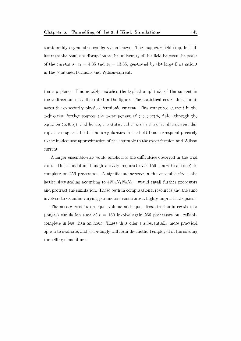
Chapter 6. Tunnelling of the 3rd Kind: Simulations 145
considerably asymmetric con�guration shown. The magnetic �eld (top, left) il-
lustrates the resultant disruption to the uniformity of this �eld between the peaks
of the current at z1 = 4.35 and z2 = 13.35, generated by the large �uctuations
in the combined fermion- and Wilson-current.
the x-y plane. This notably matches the typical amplitude of the current in
the x-direction, also illustrated in the �gure. The statistical error, thus, domi-
nates the expectedly physical fermionic current. This computed current in the
x-direction further sources the x-component of the electric �eld (through the
equation (5.40b)); and hence, the statistical errors in the ensemble current dis-
rupt the magnetic �eld. The irregularities in the �eld thus correspond precisely
to the inadequate approximation of the ensemble to the exact fermion and Wilson
current.
A larger ensemble-size would ameliorate the di�culties observed in the trial
case. This simulation though already required over 156 hours (real-time) to
complete on 256 processors. A signi�cant increase in the ensemble size � the
lattice sites scaling according to 4NEN1N2N3 � would entail further processors
and protract the simulation. These both in computational resources and the time
involved to examine varying parameters constitute a highly impractical option.
The ansatz case for an equal volume and equal discretization intervals to a
(longer) simulation time of t = 150 involve again 256 processors but reliably
complete in less than an hour. These thus o�er a substantially more practical
option to evaluate; and accordingly will form the method employed in the ensuing
tunnelling simulations.

Chapter 6. Tunnelling of the 3rd Kind: Simulations 146
6.4 Renormalization
6.4.1 Numerical Renormalization Procedure
Renormalization essentially implies that the potentially observable quantities in
the quantum system prior to implementation of the procedure include an unphys-
ical component. This component occurs through the correlator mode-expansion
involving a non-convergent integrand. In the continuum, the integration of this
integrand over all modes produces an in�nite result. The restriction to a �nite
number of modes on the lattice ensures a �nite result. Reducing the lattice
spacing on a �xed physical length, though, increases the number of modes in
the summation and, hence, the non-convergence of the additional contributions
causes the summation to diverge. Any physical observable may reasonably be
assumed to remain independent of the lattice parameters. This, hence, implies
the divergence on the reduction of the lattice spacing results entirely through
the unphysical contribution to the correlators. (In practice, the physical vari-
ables converge to a constant value, rather than remaining strictly invariant, on
reducing the lattice spacing. The convergence of the results to a su�cient degree,
though, may ensure the physical values remain constant to an arbitrarily high
accuracy on changing the spacing. This hence enables distinguishing any much
larger, unphysical contributions.) The correlator, prior to any renormalization,
thus includes both this physical component, invariant on the reduction in lat-
tice spacing, and the unphysical contribution dependent on the lattice spacing.
This in particular implies that the combined fermion- and Wilson-current on the
lattice, without renormalization, likewise involves both these contributions:
jf (X,∆x) ≡(q
~Im{〈 ˆΨ(X)γ1U1(T,X3)Ψ(X + 1)〉
}− q
~rwIm
{〈 ˆΨ(X)U1(T,X3)Ψ(X + 1)〉
})∣∣∣∣∆x
= jphys(X) + jdiv(X,∆x).

Chapter 6. Tunnelling of the 3rd Kind: Simulations 147
Obtaining the renormalized dynamics hence e�ectively entails subtracting the
spacing-dependent contribution in the fermion current.
The invariance of the physical component at di�ering lattice spacing implies:
jdiv(X,∆x) = jf (X,∆x)− jf (X,∆xref ) + jdiv(X,∆xref );
thus expressing the renormalizable contribution at any lattice spacing through the
fermionic current at the selected reference-spacing. Further, the �eld renormal-
ization in principle results through adding contributions in the action constructed
through a coordinate-independent variable multiplying the existing terms; and
these factors accordingly modifying the corresponding components in the dynam-
ics. These additional terms may reasonably be derived from the multiplying of
the plaquette terms � de�ning the discrete equivalent to the electromagnetic �eld
tensor � in the action (5.32) on the lattice:
1
c∆V
[αE∑i
~2
2qµ0(∆xi)2(∆x0)2(2− Ui0(X)− U0i(X))
− αB∑ij
~2
4q2µ0(∆xi)2(∆xj)2(2− Uij(X)− Uji(X))
].
The �rst summation, on varying the action and applying the ansatz, corresponds
to additional terms (on the non-zero side) in the electric �eld dynamics (5.58),
identical to the existing electric �eld contribution except with the renormalization
coe�cient αE multiplying the �eld:
αE1
∆x0
1
µ0c(E1(T,X3)− E1(T − 0, X3)) .
Likewise, the second summation yields additional terms in the electric �eld dy-
namics, identical to the existing plaquette terms � corresponding to the magnetic
�eld in the continuum limit � except with the renormalization coe�cient αB mul-
Chapter 6. Tunnelling of the 3rd Kind: Simulations 148
tiplying each term2:
αB1
∆x1(∆x3)2
~qµ0
Im {U13(T,X3)− U31(T,X3 − 3)} .
An identical renormalization coe�cient may be chosen, for simplicity, in both
the additional contributions to the action: αE ≡ αB ≡ α. This single factor α
may specify the renormalization factor multiplying both the electric and plaque-
tte term3.
For the renormalization terms to cancel the divergent contribution to the
current in the electric �eld dynamics, hence, implies these opposing components
relate through
jdiv(X,∆x) =
α
(1
∆x0
1
µ0c(E1(T,X3)− E1(T − 0, X3))
+1
∆x1(∆x3)2
~qµ0
Im {U13(T,X3)− U31(T,X3 − 3)}). (6.1)
This expression for the divergent contribution, further, involves purely �xed pa-
rameters, the discretized electromagnetic �elds and the renormalization coe�-
cient. The requirement for physical observables to essentially remain indepen-
dent of lattice spacing, further, applies to the discrete electric �eld and plaquette
terms inside the bracket, respectively corresponding to the time derivative of
the electric �eld and of the spatial derivative of the magnetic �eld. Any lattice
spacing dependency in the renormalization current therefore occurs within the
renormalization coe�cient; and the coordinate independence of the coe�cient
determines the spatial variation of the renormalization piece occurs entirely in
2These additions to the action notably also will contribute to the Gauss'-law constraint onthe lattice (5.55); consideration of this is not necessary to obtain the correct dynamics of thesystem.
3This contrasts the more complicated choice examining distinct factors in the analytic cal-culation.
Chapter 6. Tunnelling of the 3rd Kind: Simulations 149
the electric �eld and plaquettes:
jdiv(X,∆x) =
α(∆x)
(1
∆x0
1
µ0c(E1(T,X3)− E1(T − 0, X3))
+1
∆x1(∆x3)2
~qµ0
Im {U13(T,X3)− U31(T,X3 − 3)}). (6.2)
This, thus, provides the expressions for determining the renormalization co-
e�cient. The renormalization procedure correspondingly involves evaluating the
unrenormalized current minus this contribution in the electric �eld dynamics
(5.58). This e�ectively implies modifying the equation to include a factor of
1 +α(∆x) multiplying each electric �eld term and plaquette to, thus, obtain the
renormalized dynamics.
6.4.2 Evaluating the Renormalization
Considering the expression (6.2) in the simple case involving a static state and
the magnetic gradient identical with both the lattice spacings therefore yields
α(∆x) = ∆x1(∆x3)2 qµ0
~jf (X,∆x)− jf (X,∆xref )
Im {U13(T,X3)− U31(T,X3 − 3)}+ α(X,∆xref ).
This, thus, determines the renormalization coe�cient at any lattice spacing. The
evaluation involves measuring the unrenormalized current at both the relevant
scale and at a reference lattice spacing for an identical, set magnetic �eld in both
cases, with also the renormalization coe�cient speci�ed at the reference lattice
spacing.
This reference coe�cient forms a constant addition to the expression, and
correspondingly to the unrenormalized current at any scale. The (unphysical)
divergence in the current, thus, occurs independently of this piece. This, there-
fore, implies the precise value of this term may simply be ignored for obtaining

Chapter 6. Tunnelling of the 3rd Kind: Simulations 150
the physical, convergent current4. Alternatively, this constant piece may be con-
sidered to arbitrarily de�ne the scale of the renormalization and accordingly the
value simply set at the reference lattice spacing to de�ne the renormalization
scheme. The simplest case may therefore impose the coe�cient at the reference
scale to equal zero.
Obtaining the convergence in the current regardless may thus result on de-
termining the renormalization coe�cient speci�ed through
α(∆x) = ∆x1(∆x3)2 qµ0
~jf (X,∆x)− jf (X,∆xref )
Im {U13(T,X3)− U31(T,X3 − 3)}+ α(X,∆xref ),
(6.3)
and the corresponding physical current replacing the bare current in the dynamics
may fully specify the renormalization scheme to yield the physical dynamics.
To obtain the renormalization coe�cient may in practice be accomplished
through simulating the fermion and gauge-�eld evolution (without the Higgs-
superconductor) from the initial vacuum-con�guration to the �nal static state.
Setting the gauge �eld manually ensures an identical magnetic gradient in each
case. A simple scaling in time may uniformly multiply the �nal con�guration
to increase the �eld from zero to the �nal static, state; in particular the scaling
(5.84) may provide a smooth variation5.
4A standard interpretation of the renormalization procedure considers the process to modifythe coupling constant in the system. The particular expression of the gauge terms in this systemexcludes an explicit coupling constant multiplying the gauge-�eld tensor in the action. A simple�eld rede�nition though may produce this form in an equivalent action, and hence the additionof renormalization terms multiplying the �eld tensor may be factorized to form a single, newcoe�cient. This factor thus incorporates the renormalization coe�cient; and the resultantterm multiplying the �eld tensor de�nes e�ective coupling. Determining the precise value ofthe renormalization coe�cient therefore determines the e�ective coupling; the neglecting ofthe constant contribution to the renormalization coe�cient thus simply prevents the precisedetermination of the e�ective coupling constant in the system.
5The electric �eld de�nition on the lattice implies the time-varying gauge �eld forms a non-zero electric �eld, ultimately vanishing in the �nal, static state. This time -variation, thus,models a damping of the electric �eld in the evolution to the �nal state.Imposing the tanh variation in the continuum, further, implies the resultant electric �eld
varies proportionally to sech2 (tan (πt/τ − π/2)). Hence in the limit t → τ , the electric �elddecays approximately exponentially. The �nal decay in the equivalent discrete-case, notablytherefore, models an exponentially-damped �eld.Further, the sech variation at times close to zero determines the electric �eld increases ap-

Chapter 6. Tunnelling of the 3rd Kind: Simulations 151
The static solution to the pure gauge-dynamics in the continuum � omitting
the Higgs-�eld, fermion and Wilson currents � readily provides a suitable analytic
expression for the �nal gauge-�eld. This con�guration reasonably approximates
the result on the lattice in the full dynamical case including also the (expectedly
perturbative) fermionic currents.
Substituting the chosen form (5.83) of the external current into the conse-
quent dynamics in particular determines the �nal state:
1
µ0∂3B2(t, x3) =
1
µ0∂2
3A1(t, x3) =
|J | exp
(−(X3 − z1)2
2σ2
)− |J | exp
(−(X3 − z2)2
2σ2
).
Integrating this expression once hence determines
B2(t, x3) = ∂3A1(t, x3) =
µ0
√π
2σ|J |
[erf
(−(X3 − z1)2
2σ2
)− erf
(−(X3 − z2)2
2σ2
)]+BC . (6.4)
The condition on the magnetic �eld to form anti-symmetrically in the two,
separate regions between the external currents on the periodic boundaries (see
Section 5.7) constrains the arbitrary constant. For the current peaks positioned
to divide the periodic z-axis into two equal regions, simply subtracting half the
maximum height of the combined error function pieces yields a suitably sym-
metric form: the error functions matching the requisite symmetry except about
proximately exponentially in the continuum; and accordingly the discrete analogue models asimilarly smooth increase in the initial electric �eld on the lattice.

Chapter 6. Tunnelling of the 3rd Kind: Simulations 152
the half-maximum value rather than zero. This thus determines the constant
satis�es
BC = −µ0
√π
8σ|J |
[erf
(−(zM − z1)2
2σ2
)− erf
(−(zM − z2)2
2σ2
)],
zM =z1 + z2
2.
Integrating the resultant expression again hence determines
A1(t, x3) =
µ0
√π
2σ|J |
[(X3 − z1) erf
(−(X3 − z1)2
2σ2
)− (X3 − z2) erf
(−(X3 − z2)2
2σ2
)
+
√2
πσ exp
(−(X3 − z1)2
2σ2
)−√
2
πσ exp
(−(X3 − z2)2
2σ2
)]+BCX3 +AC .
The symmetry constraint on the magnetic �eld further indicates the gauge
�eld ranges between equal and opposite values. This, hence, constrains the half-
maximum value to zero. Subtracting the value at the location X3 = zM midway
between the current peaks correspondingly imposes the constraint and thus sets
the second integration constant. This therefore fully de�nes the express analytic
form of the gauge �eld in the �nal, static state.
Figure 6.2: The magnetic �eld (left) and gauge �eld (right) evaluated analytically
for calculating the renormalization coe�cient.

Chapter 6. Tunnelling of the 3rd Kind: Simulations 153
This gauge-�eld con�guration and the tanh prefactor thus together provide
the analytic expression of the magnetic �eld to determine the renormalization
coe�cients numerically.
Setting the current width to satisfy 2σ2 = 1, for simplicity, and choosing the
amplitude J to set the magnitude of the analytic magnetic �eld to Bmax = 1.0
(comparable to the subsequent, fully-dynamical simulations) in the analytic ex-
pressions generates the �nal gauge �eld and corresponding magnetic �eld, shown
in �gure 6.2.
Figure 6.3: The fermionic current in the x-direction generated by the analytically
set gauge-�eld for ∆x1 = 0.4 (blue), 0.3 (black), 0.2 (red) with ∆x2 = ∆x3 = 0.3
and the physical volume constant; ∆x0 = 0.002, |J | = 1.
Determining the renormalization coe�cients consequently for di�ering ∆x1
demonstrates the e�ectiveness of the renormalization scheme. Setting the lattice
spacing in the x-direction separately to ∆x1 = 0.4, 0.3, 0.2 while �xing ∆x2 =
∆x3 = 0.3 and in a �xed physical volume of Lx = Ly = 9.6 and Lz = 24
produces the unrenormalized fermionic current � including both the fermion and
Wilson parts � illustrated in the �gure 6.3. Choosing the combined fermion-

Chapter 6. Tunnelling of the 3rd Kind: Simulations 154
and Wilson-current generated at ∆x3 = 0.3 to provide the reference with the
determined magnetic gradient and the measured current substituted into the
expression (6.3) hence yields the renormalization coe�cients.
Figure 6.4: The fermionic current in the x-direction in the fully-dynamical sim-
ulations without renormalization (top) and with renormalization (bottom) for
∆x1 = 0.4 (blue), 0.3 (black), 0.2 (red) with ∆x2 = ∆x3 = 0.3 and the physical
volume constant; ∆x0 = 0.002, |J | = 0.5 and ζ = π/6.
Chapter 6. Tunnelling of the 3rd Kind: Simulations 155
The coe�cient in principle is coordinate independent; in practice though,
numerically determined value varies both in time and along the z-direction. Av-
eraging the unrenormalized current over times much longer than the typical tem-
poral �uctuations though helps reduces this random error. The peaks in the
external current o�er a de�nite and distinctive location for determining the pre-
cise coe�cient-value; while the anti-symmetry in the peak locations implies the
averaging the coe�cient evaluated at both peaks may help further reduce the
error. These peak values though notably occur at sites o� the lattice and hence
the simulations provides no direct measure of the unrenormalized-current at this
location. Obtaining the numerically measured current at the two adjacent sites
of the peak provides a simple alternative while retaining the distinction and def-
initeness of the location. The time-averaged value of the current at these four
sites and the average of the corresponding coe�cients in the physical current
therefore fully de�nes the renormalization procedure.
For the cases ∆x1 = 0.2, 0.4, this yields respectively α = −0.000265269471
and α = 0.00026365064. Implementing these renormalization parameters in the
equivalent fully-dynamical case (for the respective lattice spacings with both the
volume and time-step identical to the manual analysis) yields the renormalized
current illustrated in �gure 6.4, bottom. A comparison of the renormalized cur-
rents to the unrenormalized current (top) in �gure 6.4 � especially at the peaks
(coincident with the peaks in the external current) � clearly demonstrates the
procedure e�ectively eliminates the lattice-dependent divergence. The concomi-
tant magnetic �eld in the renormalized case further con�rms the e�ectiveness:
the �gure 6.5 demonstrates the closely distributed values of the �eld after renor-
malization.

Chapter 6. Tunnelling of the 3rd Kind: Simulations 156
Figure 6.5: The magnetic �eld in the dynamical simulations with renormalization
for ∆x1 = 0.4 (blue), 0.3 (black), 0.2 (red) with ∆x2 = ∆x3 = 0.3 and the
physical volume constant; ∆x0 = 0.002, |J | = 0.5 and ζ = π/6.
These example cases, con�rming the convergence in the observable values,
therefore validate the selected lattice-parameters and the corresponding renor-
malization coe�cient for examining the superconducting system. In particular,
the parameters setting the lattice spacing equally to 0.3 where also α = 0 are
chosen for simplicity throughout the subsequent simulations.
6.5 Tunnelling System on the Lattice
6.5.1 Wall Parameters
Fixing the skin width of the barriers to smaller than the lattice spacing and the
thickness of each to d = 1.5 forms the narrowest feasible barrier � only �ve sites,
for the chosen lattice spacing � to reliably examine the transmission through the
barrier. This, in particular, includes a region on the lattice entirely within the
barrier and not purely on the surface, to examine the transmission without simply
Chapter 6. Tunnelling of the 3rd Kind: Simulations 157
examining any surface e�ects. The minimizing of the barrier thickness further
ensures the maximum potential to observe the fermionic tunnelling. Setting
the separation of the barrier centres to S = 5.7 prevented an overlap of the the
edges for the barrier thickness chosen. This also created a reasonably sized region
(larger than both the skin width, δ < 1 and the chosen thickness d = 1.5) enclosed
between the barriers where the magnetic �eld transmitted through the sheets
could form without further interference of the barriers. Positioning the barriers
centrally between currents (see Section 5.7.2) requires setting the midpoint of
the barriers to M = N3∆x3/2 = Lz/2 for the choice of length Lz on the lattice.
This, for simplicity, creates an identical region where the magnetic �eld may form
between the current and barrier on both sides external to the enclosed volume
6.5.2 Lattice Parameters
Implementing the renormalized dynamics for the lattice spacing ∆x1 = ∆x2 =
∆x3 = 0.3 in the volume of length Lx = Ly = 9.6 and Lz = 18 with the
Neumann boundaries forms the discretized system for examining transmission
through the the superconducting barrier. The chosen length in the z-direction
further o�ered su�cient space to produce an almost uniform magnetic �eld in
the region between the barrier and the external-current width with a region to
examine the �eld penetrating the barrier: the �gure 6.6 (top) shows a typical
con�guration in the static state.
Setting ∆x0 = 0.002 provided time-step necessarily smaller than the lattice
spacing and su�cient to readily yielding convergence in the observable param-
eters; while setting τ = 80 to transition from the vacuum to the static state
further provided a practicably brief transition with negligible transient features
perturbing the static state.
The lattice discretization intervals, further, involved a total number of lattice
sites readily implemented on a computer; while this total lattice size, along with
the choice of temporal discretization-interval and the brief initial-increase time
Chapter 6. Tunnelling of the 3rd Kind: Simulations 158
ensured numerical evaluation within a practicable time-frame.
6.5.3 Typical, Magnetic-Field Transmission
Setting the external-current magnitude to |J | = 0.5 with the width σ = 0.8/√
2
while varying the squared wall-strength through η = [2, 7.5] in half-integer incre-
ments will provide the speci�c con�guration for examining the transmission on
varying the wall strength.
The analytical estimates indicating the bound for detecting the tunnelling sig-
nal (Section 5.3) determines the maximum wall-strength. Examining the trans-
mission, therefore, up to η = 7.5 will su�ciently encompass the region where the
tunnelling signal is expected to dominate.
Choosing the increase in the external current to the �nal, maximum ampli-
tude in a time τ = 80 produces increasing �elds until this time. The generated
electromagnetic waves subsequently decay: their amplitude rapidly negligible,
with the damping coe�cient set to ζ = 6π/35. This hence generates the essen-
tially static, �nal state before X0 = 150, when the resultant �elds are examined.
The �gure 6.6, top illustrates the typical magnetic �eld variation in the static
state: the �eld strongly decays through even the narrow wall to a magnitude
several orders smaller in between the superconducting barriers.
A signi�cant Higgs current also occurs within the wall: the �gure 6.6, bottom
demonstrates the typical form. The Higgs current varies essentially ∝ A1ρ2;
hence, the decrease in the current occurs, essentially, due to the decay in the
gauge-�eld, while the sharp peak at the boundary results through the almost step-
function variation in ρ. This current also notably acts in accordance with Lenz's
Law to essentially oppose the magnetic �ux generating the current: the current
aligns in the negative x-direction to form a magnetic �eld counteracting the gauge
�eld generated by the external current. The Higgs current, in the absence of any
fermion contribution, notably coincides with the several orders decrease in the
magnetic amplitude through the barrier; the current, thus, corresponds to the

Chapter 6. Tunnelling of the 3rd Kind: Simulations 159
Figure 6.6: The typical magnetic �eld (top) and Higgs-current (bottom) without
fermions (left) and with fermions (right) in the presence of the superconducting
barrier (grey-shaded region): |J | = 0.5, η2 = 8.
purely classical decay in the magnetic �eld.
This strong decay in the magnetic �eld notably results both with and with-
out the fermions: the �gure 6.6, top and right incorporating fermions and the
case excluding fermions in �gure 6.6, top and left demonstrate the typical simi-
larity. The Higgs superconductor-current, both with and without fermions, thus
produces the most substantial change in the magnetic �eld.
A comparably small fermionic current results within the barrier: the �gure 6.7
illustrates the fermions within the barrier typically generate a combined fermion-
and Wilson-current several orders of magnitude smaller than the Higgs current.
The fermionic current thus forms a sub-dominant e�ect in the �eld decay.
This current may, nonetheless, generate a signi�cant contribution to the

Chapter 6. Tunnelling of the 3rd Kind: Simulations 160
Figure 6.7: The typical fermion current in the presence of the superconducting
barrier (grey, shaded region): |J | = 0.5, η2 = 8.
transmission where the resultant change in transmission becomes comparable
to the classical transmission. The typical fermion contribution forms an addi-
tional current opposing the Higgs current within the barrier. This fermionic
contribution, hence, counteracts the Higgs-�eld suppression of the magnetic �eld
to increase the magnetic transmission. The fermion current, moreover, comprises
the fermions formed within the barrier and therefore e�ectively includes the par-
ticles contributing to the tunnelling. These particles, in counteracting the Higgs
suppression to increase the transmission, thus act in qualitative accordance with
the tunnelling e�ect. Both the fermion and Higgs current within the barrier vary
on the change in the barrier strength and thus complicate the precise correspon-
dence between the fermionic current and the tunnelling amplitude. Examining
the magnetic transmission, regardless, may enable measurement of the resultant
tunnelling.
The fermionic current, further, at the boundaries acts in accordance with
Lenz's Law. These currents, thus, align opposite to the external current and,

Chapter 6. Tunnelling of the 3rd Kind: Simulations 161
hence, generate a magnetic �ux opposing the �eld corresponding to the external
current. Increasing the wall strength without fermions also, notably, alters the
magnetic �eld amplitude in the regions between the boundary and superconduc-
tor. This variation in the presence of fermions, reacting to the external current
in accordance to Lenz's Law, causes the induced fermion current to generate a
magnetic �ux, varying on the change in wall strength. The resultant magnetic
�eld in the regions between boundary and the superconductor thus varies on the
change in wall strength, both with and without fermions; and the resultant �elds
di�er in the case with fermions, compared to the equivalent case without the
fermions.
This variation in the external magnetic �eld, thus, prevents a direct compar-
ison between the �eld transmission on varying the wall strength or on including
the fermions. Forming the ratio of the central value between the superconducting
barriers, to a representative �eld-value external to the superconducting enclosure
provides an equivalent variable for directly comparing the di�ering cases:
BR =Bint
Bext. (6.5)
To attribute the variation in this ratio purely to the changes in wall strength
and the presence (or absence) of fermions neglects the potentially complex varia-
tion in the transmitted electric �eld related simply to the changes in the external
�eld. This variation, though, may approximate a linear relation over a su�ciently
small range in the external �eld. The ratio in this limit meaningfully comprises
the proportionality constant distinguishing the linear relation; and, thus, within
the linear regime, represents the transmission independently of the precise exter-
nal �eld. Examining a common range of the external �eld in each case, further,
forms a suitably equivalent context for comparison.
The magnetic �eld halfway between each boundary and the adjacent wall
provides a de�nite representative-value external to the superconductor within

Chapter 6. Tunnelling of the 3rd Kind: Simulations 162
the accurately-uniform region; while the symmetry in the system implies an
identical magnetic �eld forms at these two positions. Averaging the �eld at both
locations, hence, may reduce the computational error in the measured exterior
�eld-value. Selecting the central �eld value between the superconducting barrier
may provide a de�nite, distinctive location to measure the transmitted magnetic
�eld.
These speci�ed positions, though, in practice, may occur o� the de�ned
lattice-sites. The only minor deviation from uniform over a wide region external
to the superconductor ensures in this case that the �eld value at the adjacent
sites provides a highly similar value to the �eld at the o�-lattice site; and thus
essentially yields an equally-representative value of the �eld external to the su-
perconductor. Selecting, in particular, the �eld value at the adjacent site closest
to the boundary when the de�ned external-location occurs o� the lattice, there-
fore, provides the external-�eld values to average. Comparing these in each case
to the �eld at the adjacent site, but nearer the barrier, and assuming a smooth
variation in the �eld between the lattice sites may, hence, provide an upper bound
on the deviation between the �eld at the speci�ed site and the measured value
at the adjacent site nearer the boundary. The magnitude of this di�erence for
each case in the subsequent data set to measure the tunnelling (�gure 6.9) equals
∼ O(10−5) per cent of the representative value used in computing the transmis-
sion. This con�rms the chosen, adjacent site provides a highly comparable value
to the true measurement at the de�ned location, o� the lattice; the measured
�eld, therefore, forms an equally suitable, representative value for examining the
transmission ratio.
The �eld value inside the superconducting enclosure also varies very little;
hence, the values at the adjacent sites to the midpoint between the barriers,
when the midpoint occurs o� the lattice may provide a suitably-representative
value of the internal �eld. Further, the symmetry in the system implies the
�eld at these sites are equal, and thus either value may equivalently de�ne the

Chapter 6. Tunnelling of the 3rd Kind: Simulations 163
internal value. Averaging the pair therefore technically reduces the error in this
representative value. These �eld values thus practically de�ne the internal and
external �elds examined on the lattice.
Varying the current through the range |J | = 0.5, 0.5 + 5 · 10−5, 0.5 + 5 ·
10−4, 0.5+5·10−3 for a �xed wall-strength produces a variable, external � and cor-
respondingly varied, internal � magnetic �eld. Calculating the linear-regression
�t to these correlated variables, hence, yields the proportionality constant de-
scribing the magnetic transmission.
The �gure 6.8 shows the typical ratio and linear regression both with and
without fermions for the examined wall-strengths within a common range of the
external �eld.
Figure 6.8: The typical variation in magnetic �eld inside the shielded region
(Bint) on varying the uniform, external �eld (Bext) both without (left) and with
(right) fermions. These demonstrate the highly linear relation between these
�elds over approximately an order or magnitude in the external �eld.
These cases illustrate the highly linear relation between the external and
internal currents over around an order of magnitude range in the external �eld.
The wall strength and presence of fermions a�ecting the generated �eld causes
the precise range to vary within each case; but these various regimes, importantly,
include a common range.
This high linearity, therefore, con�rms the suitability of the ratio for describ-
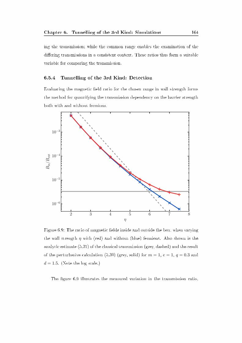
Chapter 6. Tunnelling of the 3rd Kind: Simulations 164
ing the transmission; while the common range enables the examination of the
di�ering transmissions in a consistent context. These ratios thus form a suitable
variable for comparing the transmission.
6.5.4 Tunnelling of the 3rd Kind: Detection
Evaluating the magnetic �eld ratio for the chosen range in wall strength forms
the method for quantifying the transmission dependency on the barrier strength
both with and without fermions.
Figure 6.9: The ratio of magnetic �elds inside and outside the box, when varying
the wall strength η with (red) and without (blue) fermions. Also shown is the
analytic estimate (5.31) of the classical transmission (grey, dashed) and the result
of the perturbative calculation (5.30) (grey, solid) for m = 1, e = 1, q = 0.3 and
d = 1.5. (Note the log scale.)
The �gure 6.9 illustrates the measured variation in the transmission ratio.
Chapter 6. Tunnelling of the 3rd Kind: Simulations 165
Both the case with (red line) and without (blue line) fermions, for low wall
strengths of η . 5 produce e�ectively identical transmission. This indicates the
classical transmission dominates within this regime of wall strength. The �gure
also shows the simplistic heuristic guide (grey, dashed line) for comparison. This
simple estimate di�ers in the absolute value; the discrepancy, though, is expected
to result, considering the classical guide neglected both the �nite volume and dis-
cretization e�ects on the transmission in the fully dynamical simulations (see also
the discussion on this in Section 5.3). The simulation results in the weak barrier
regime, nonetheless, notably form the exponentially decaying relation predicted
in the simplistic, classical estimate: thus, further con�rming the dominance of
classical e�ects within this regime.
Signi�cant di�erences in the measured transmission with the fermions, com-
pared to without begin where η ≈ 5. The increasing barrier strength produces a
progressive decrease in the case without fermions, while the system with fermions
begins to asymptote to a value around 2 · 10−6. This indicates the quantum in-
teraction a�ect the system more markedly within this regime of barrier strength.
The computed transmission without the fermions also noticeably grows to val-
ues larger than continued exponential decreasing transmission predicted through
the simple guide. This may simply result since the measured external �eld is
lower than the actual magnetic �eld strength incident on the barrier.
Although the magnetic �eld forms a predominantly level region outside the
superconducting enclosure (see �gure6.6 for an illustrative case), the magnetic
�eld, actually, increases slightly towards the barrier. This rise, thus, implies an
increased in the �eld of Berr ∼ O(10−5) incident on the barrier, compared to the
measured external-�eld, at the position only partway between the boundary and
the wall (see Section 6.5.3). The stronger magnetic �eld incident on the barrier
causes a larger, classical transmission compared to the classical estimate for the
measured external �eld. This may, hence, signi�cantly increase the measured
transmission-ratio without fermions, compared to the classical guide where the

Chapter 6. Tunnelling of the 3rd Kind: Simulations 166
discrepancy in the ratio matches the order of the classical estimate. Examin-
ing the classical estimate (5.31) determines the increased, incident �eld value of
Berr ∼ O(10−5) yields an approximately O(10−4) increased transmission ratio
for the measured external �eld value of Bext ∼ O(10−1) (see the �gure 6.6 for
an illustrative case), in contrast to the classical estimate for the measured ex-
ternal value. (The consequent variation is also reasonably assumed, simply, to
superimpose on the �nite volume and discretization e�ects expected to alter the
classical guide � and evidenced for the low barrier-strengths.) This, therefore,
indicates the discrepancy in the incident �eld generates a signi�cant a�ect where
η & 4 and this e�ect grows. The measured transmission-ratio without fermions,
notably, increases slightly at η ∼ 4, to a slower decay compared to the strictly
exponential form, predicted in the classical estimate; and this grows on increas-
ing wall-strength until the transmission ratio exceeds the classical guide. These
deviations, thus, match the discrepancy expected simply through the di�erence
in the incident �eld on the wall and the measured external value.
The classical estimate indicates the magnetic transmission tends to zero on
increasing barrier strength, irrespective of the magnitude of the external �eld.
This implies any contribution independent of wall strength will dominate for
su�ciently high wall strength. The decay to zero of the classical transmission,
thus, assures the asymptoting to a �xed value for η & 5 in the simulations
with fermions results through the quantum contributions to the transmission.
This asymptotic value equal to around 2 · 10−6, moreover, matches the analytic
result (grey, solid line) to within the expected factor of two. The numerical
transmission, though, notably, tends to a value slightly lower than the analytic
estimate. This may result through the measurement of the magnetic �eld at
a �nite distance inside the enclosure. The analytic calculation evaluates the
tunnelling expectation in�nitely far from the barrier, where the entirety of the
fermions tunnelling through the barrier may be expected to have (re-)combined
to generate magnetic �eld. In contrast, the simulations measure the magnetic

Chapter 6. Tunnelling of the 3rd Kind: Simulations 167
�eld near the barrier, compared to the width of the barrier. The �nite fermion
current (if smaller than visible on the scale for the illustrative case in �gure 6.7)
generated inside the superconducting enclosure, from an initial absence of current
in the vacuum, indicates a small portion of the fermions having tunnelled through
the barrier remain to (re-)combine into magnetic �eld. These fermions, hence,
reduce the transmitted �eld compared to the complete conversion expected at
in�nite distance and, thus, may cause the slightly lower measured value of the
tunnelling contribution.
Repeating the analysis, using di�erent lattice spacings, for a �xed physical
volume and �xed couplings may provide a quantitative estimate of the numerical
error in the measured transmission. The variation in the observed �elds on the
change in lattice spacing would indicate the dependence of the discretization er-
rors on the lattice spacing. Evaluating this error for the lattice spacing in the sim-
ulation, hence, would provide a quantitative measure of the discrepancy between
the computed and analytic estimates resulting simply through discretization; any
remaining deviation might be attributed to physical e�ects. This computationally
intensive analysis to compute the numerical errors in the transmission, currently
though, remains a work to complete. The discrepancies without distinguishing
the numerical errors, notably, nonetheless, match the qualitative expectation on
considering the physical e�ects in the system. This provides assurance the results
accurately demonstrate the physical, �eld transmission.
The strong deviation in the case on incorporating fermions, compared to
without, and the transmission ratio asymptoting to a constant, slightly below the
analytically determine value, therefore, forms a reasonable con�rmation of the
analytic estimate. This result likewise indicates the measured fermionic current
includes the tunnelling fermions and, thus, the dynamical system incorporates
the tunnelling of the 3rd kind.
Chapter 6. Tunnelling of the 3rd Kind: Simulations 168
6.5.5 Conclusion
The work in this chapter has, in summary, developed and re�ned the techniques
for examining tunnelling of the 3rd kind in real-time simulations. This distinct
form of tunnelling provides a potentially interesting application of quantum �eld
e�ects in a laboratory arrangement. The simulations have examined this phe-
nomenon in an idealized laboratory scenario where two parallel and in�nite su-
perconducting planes shield a central region from the uniform magnetic �eld in
the regions to either side. These superconducting sheets strongly suppressing
the magnetic transmission form the classical barrier to the external magnetic
�eld. The simple estimate of this e�ect predicted the exponential decay in the
transmission. Incorporating the quantum e�ects also enables the magnetic �eld
external to the barrier to convert into fermionic particles. These cross unhindered
through the barrier with the subsequent annihilation (re-)creating the magnetic
�eld. This tunnelling of the 3rd kind thus contributes to the magnetic transmis-
sion through the barrier. The perturbative calculation of this e�ect implies the
resultant transmission equals only around 3.4 · 10−6 times the external �eld with
a possible correction to this by a factor between one to two � accounting for the
di�erences between the analytic calculation and the numerical simulation. This
e�ect becomes detectable only where the superconductors reduce the classical
transmission to less than the tunnelled component. The combination of the clas-
sical decay and the tunnelling e�ected together formed the basic estimate for the
expected transmission both with and without the fermions.
These results matched the dynamical simulations with signi�cant accuracy.
The decay on increasing wall-strength without fermions qualitatively reproduced
the estimated exponential-decrease to reasonable precision; though, the absolute
numerical values were signi�cantly less than the analytic estimate. This discrep-
ancy likely resulted through the intricacies involved in implementing the results
in the �nite volume on the lattice, unaccounted for in the simple estimate. The
Chapter 6. Tunnelling of the 3rd Kind: Simulations 169
transmission without fermions also demonstrated a slightly slower than exponen-
tial decay where η & 5. This simply occurred through the consistently larger
�eld incident on the barrier compared to the measured external �eld generat-
ing a signi�cant increase in the transmission for the larger wall strengths. The
tunnelling signal of Bin/Bout ≈ 2 · 10−6, signi�cantly, equalled the perturbative
estimated within the expected correction factor. Determining the discretization
errors in the result may be accomplished on the repetition of the simulation us-
ing di�erent lattice sizes, for a �xed physical volume and �xed couplings. This
may enable quantifying the lattice spacing errors and, correspondingly, distin-
guishing the genuine physical discrepancies between the numerical results and
the analytic estimates. The qualitative consistence in the discrepancies to the
expected deviation, nonetheless, validated the physical nature of the computed
transmission. These results, therefore, provided a reasonable con�rmation of
the tunnelling-e�ect, and the perturbatively calculated transmission signal. The
successful implementation of the system indicates, further, the potential for real-
time simulations of fermionic systems to produce accurate predictions for testing
in the laboratory.
This numerical simulation of tunnelling were accomplished on applying the
established techniques for dynamical fermions to the idealized experimental ar-
rangement. The ensemble method o�ered a possible procedure to solve the dy-
namics analogously to the oscillon system. This essentially involved the statisti-
cal average of ordinary numbers replacing the ladder operators for evaluating the
fermionic correlators. The method required an additional set of �elds in contrast
Chapter 6. Tunnelling of the 3rd Kind: Simulations 170
to the purely bosonic case. These �male� and �female� �elds respectively were of
the form
ΨM,c(x) =
√~c2Vx∑s
∑K
∆k1
2π
∆k2
2π
∆k3
2π
1
2ωK
[ξK,s,cψ
(U)K,s(X) + ζK,s,cψ
(V )K,s(X)
],
ΨF,c(x) =
√~c2Vx∑s
∑K
∆k1
2π
∆k2
2π
∆k3
2π
1
2ωK
[ξK,s,cψ
(U)K,s(X)− ζK,s,cψ
(V )K,s(X)
],
where the minus sign between the terms of the integrand distinguishes the two
sets. This di�erence, importantly, ensures the statistical variance of the male
and female �elds in combination can reproduce the potentially negative values
of the fermionic correlators.
The ensemble method for the fermions � equivalently to the oscillon case �
o�ered the possibility to reduce the computational requirements. This method,
in principle, entails in�nitely many �elds to precisely reproduce the quantum
correlators. The use, though, of a �nite ensemble, in practice, may adequately
approximate the correlators. Had this �nite ensemble in the fermionic system
involved fewer �elds than the total modes in the 3 + 1D system, the ensemble
technique may have o�ered the possibility to readily evolve the system. The trial
simulation involving the male and female �elds, though, indicated a small en-
semble, equal to two and a half per cent of the total modes, produced substantial
statistical-noise in the fermionic current; this strongly distorted the formation
of the uniform magnetic �eld. This demonstrated the need for a much larger
ensemble size to accurately evolve the fermions. The comparatively small ensem-
ble in the trail case also required over 156 hours (real-time) to simulate. This
indicated the impracticable times required for the larger ensemble and therefore
the unsuitability of this method for simulating the system.
Imposing the symmetries of the system explicitly on the �elds provided the al-
ternative method for simplifying the system. The superconducting planes aligned
parallel and extended in�nitely in the x and y directions, with the magnetic �eld

Chapter 6. Tunnelling of the 3rd Kind: Simulations 171
also aligned parallel to the planes essentially formed a homogeneous system or-
thogonal to the z-axis. This, hence, determined the ansatz for the �elds:
A1(x) = A1(t, x3), A2(x) = A3(x) = 0;
j1(x) = j1(t, x3), j2(x) = j3(x) = 0;
θ(x) = 0;
ψ(U/V )(k1,k2,λ,s)
(x) = eik1x1eik2x2χ(U/V )(k1,k2,λ,s)
(t, x3).
The ansatz e�ectively reduced the dynamical equations to a 1+1D system in the
z-direction with the quantum correlators involving a sum also over the x- and
y-directions in mode space. This produced a signi�cant decrease in the �eld val-
ues to compute on the lattice and the consequent simulation times. The ansatz
evolution typically required under an hour (real-time) for each simulation. This
greatly improved on the ensemble method timings and, moreover, provided a
practicable method for examining the tunnelling. The considerable increase in
e�ciency thus demonstrates the potential power of a suitable ansatz to signi�-
cantly reduce the computational times in fermion simulations.

Chapter 7
Summary and Outlook
This work has presented the �rst dynamical, quantum simulations of oscillons.
The precise quantum treatment of the decay substantially reduced the oscillon
lifetimes. These structures classically lasted longer than O(104 |m|−1) (while
simulations have demonstrated them to last longer than O(106 |m|−1) [37, 41,
43, 44]) and most remained beyond the end of the simulations. The structures in
the quantum evolution, in contrast, lasted less than O(103 |m|−1) with the decay
in all cases occurring before the end of the simulation. These also decayed grad-
ually: in contrast to the abrupt endpoint (at a critical frequency) in the classical
evolution. Despite the distinctly di�ering evolution, the classical and quantum
oscillons occur for similar Gaussian initial conditions. This indicated that the
Gaussian pro�les, at least during the early stage (after that initial transients),
evolve largely una�ected by the quantum �uctuations; and those con�gurations
generating oscillons only react to the quantum e�ects at later times.
The procedure to examine the quantum system employed the Hartree ap-
proximation to expand the quantum correlators. This essentially split the �eld
into the classical background and the quantum perturbation to the system with
the correlators expanded in these two �elds. The resultant correlators of the per-
turbation higher than second order were then set to vanish. This approximation
might, perhaps most evidently, be improved through expanding to higher orders
172

Chapter 7. Summary and Outlook 173
in the perturbations. An equivalent system in the 1/N approximation for the
scalar �eld likewise expanded to higher order in the perturbations may also pro-
vide an alternative method to precisely examine the quantum decay of oscillons.
These possibilities remain to be examined.
This thesis has also presented the �rst dynamical simulations to examine tun-
nelling of the 3rd kind in an idealized laboratory scenario. The system involved
two parallel, in�nite superconducting-sheets shielding a central region from the
uniform magnetic �eld in the regions to either side. These superconducting sheets
formed the classical barrier to the external magnetic �eld. Incorporating the
quantum interaction enabled the �eld to pair-create fermionic particles. These
could cross unhindered through the barrier with their subsequent annihilation
(re-)creating the magnetic �eld inside the shielded region. This tunnelling of the
3rd kind thus increased the transmission through the barrier.
The measurements of the transmitted �eld in the dynamical simulations re-
markably accurately con�rmed the simple, analytic estimates. These dynamical
results qualitatively reproduced the exponential decrease estimated in the trans-
mission on varying the interaction strength between the barrier and the magnetic
�eld. The tunnelling signal in the transmitted magnetic �eld, moreover, equalled
approximately 2 · 10−6 per cent of the external �eld value. This matched the
analytic value, within the expected correction factor and matched the qualita-
tive deviation expected through heuristic arguments. The result, thus, provided
a reasonable con�rmation of this perturbative result.
Completing the simulations using di�erent gauge-fermion couplings (q) o�ers
a further method to test the validity of the analytic calculation. Obtaining the
predicted analytic result in the regime where the total transmission tends to a
constant value, correspondingly, would further con�rm the existence of tunnelling
of the 3rd kind.
The repetition of the analysis also, using di�erent lattice sizes, for a �xed
physical volume and �xed couplings, may provide a method to estimate the
Chapter 7. Summary and Outlook 174
discretization errors on the lattice. This, correspondingly, may ensure the dis-
tinguishing of physical e�ects in the discrepancies between the numerical results
and the simpli�ed, analytic estimates. The detailed examination may further as-
sure the dynamical system accurately encapsulates the quantum tunnelling; and
potentially also o�ers a more precise comparison to experiments, for claiming
detection of the tunnelling.
These current results successfully implementing the tunnelling of the 3rd kind,
importantly, demonstrate the potential for real-time simulations of quantum sys-
tems to produce accurate predictions for testing in the laboratory. The examined
tunnelling con�guration might most simply be adapted to examine the transmis-
sion of electromagnetic waves � this would form a version �light shining through a
wall� experiments. A perturbative calculation, in reasonable limits where the sys-
tem is tractable, predicts this case involves a frequency dependent transmission
[98]. The simulations might test the validity of this estimate; and also examine
the transmission in regimes where the analytical calculations are unable to pro-
vide explicit predictions. Preliminary trials to generate an electromagnetic wave
on the lattice with Neumann boundaries have been attempted. The Neumann
condition on the z-component of the gauge �eld, though, disrupt the correct
formation of an sinusoidal pulse on the boundaries. Overcoming this numeri-
cal di�culty remains a challenge to solve for the practicable simulation of the
sinusoidal pulses undergoing tunnelling of the 3rd kind.
These procedures developed for tunnelling, further, o�er the potential to ex-
amine the quantum hall e�ect within a (fundamental) �eld-theoretic framework
(for a detailed discussion of this quantum phenomenon, see for instance [100]).
This phenomenon occurs in a current restricted to a planar conductor with a
strong magnetic �eld perpendicular to the plane. The resistance in the direc-
tion perpendicular both to the direction of the current and to the magnetic �eld
increases stepwise on increasing the magnetic �eld strength. These step sizes
involve the ratio of the electron charge to Planck's constant either in integer

Chapter 7. Summary and Outlook 175
multiples or a limited set of fractional values. The integer values result essen-
tially through the magnetic �eld quantizing the electrons into the (quantum-
mechanical) Landau levels with the steps in the resistance corresponding to the
number of occupied Landau levels in the system. Electron-electron interactions
generate the fractional steps in the resistance although this process is much less
understood. The dynamical simulations of these systems might provide insight
into the �eld theoretic origin of the integer steps and help further explain the
nature of the fractional e�ect.
Both the scalar-�eld oscillon and the tunnelling systems demonstrated the ap-
plication of a statistical ensemble to approximate the quantum two-point func-
tions in the dynamics. This procedure for the bosonic scalar-�eld involves a
single ensemble, constructed analogously to the operator mode expansion but
where a Gaussianly-distributed number replaced the ladder operator. The sta-
tistical mean of these ordinary numbers in e�ect replaces the quantum average
of the operators in the system. This determines the statistical variance of the
ensemble �elds may replace the quantum correlators throughout the dynamics.
The statistical method likewise involves the statistical ensemble replacing the
fermionic correlators in the dynamics, except the fermionic system requires two
ensembles di�ering only in a minus sign. This crucial di�erence ensures that the
statistical variances � on forming the products of �elds in the two sets � can
reproduce the potentially negative values of the fermion correlators.
The ensemble method o�ered the possibility to reduce the total �eld values to
evolve on the lattice. This process, in the bosonic case, failed to o�er signi�cant
gains. The convergence of the scalar-�eld evolution needed an ensemble size of
M = 60000. On the square lattice of N = 256 point, this was only marginally
fewer �elds than the N2 = 65536 modes required in the mode function method.
The trial case in the fermionic system, similarly, indicated that the method re-
quired substantial computational resources and an impracticable real-time for
completion.

Chapter 7. Summary and Outlook 176
These applications demonstrate an evident limit in the e�ectiveness of the
ensemble method. The strongly inhomogeneous nature of the oscillon and the
results obtained without volume averaging� to potentially reduce the statistical
�uctuations � likely were the reasons for requiring a sizeable ensemble. These
di�culties likewise potentially also caused the ensemble method to fail in the
fermion case. The low dimensionality of the oscillon simulations also likely con-
tributed to the large ensemble-size in comparison to the number of modes. These
potential di�culties may therefore indicate that both the dimensionality and
whether the results involve volume averaging are important factors in consider-
ing the ensemble method for use in future simulations.
Constructing an ansatz for the �elds incorporating the symmetries in the
system provided an alternative method for simplifying the tunnelling dynamics.
This e�ectively reduced the system to a 1 + 1D problem in the z-direction with
the quantum correlators involving a sum also over the x- and y-directions in
mode space. This produced a signi�cant decrease in the �eld values to compute
on the lattice, and consequently enabled the evolution of the fermionic system in
a practical time.
The ansatz dynamics reliably required less than an hour for each simulation
in contrast to the more than six days in computing the trial ensemble case � still
using fewer than the necessary �elds. This considerable increase in e�ciency thus
demonstrates the potential power of a suitable ansatz to signi�cantly reduce the
computational times in fermion simulations. Using a spherically symmetric form
of the fermion spinors [101], for instance, may simplify the dynamics to enable the
completion of otherwise impracticable simulations. Devolving the techniques for
fermion �elds satisfying various symmetries, alongside the advances in computing
resources to support larger numbers of �elds on the lattice may increasingly
enable practicable simulations using the exact mode functions to examine the
dynamical evolution of fermions.

Appendix A
Neumann Boundaries: Continuum
The Neumann conditions on the z-boundaries, in the continuum (see Section
5.5.2) constrain both the gradient of the fermion current in the perpendicular
directions and also the component parallel to vanish everywhere on these bound-
aries:
iq
~∂3〈T ˆΨ(x)γ1/2Ψ(x)〉
∣∣∣x=xB
= 0, (A.1a)
iq
~〈T ˆΨ(x)γ3Ψ(x)〉
∣∣∣x=xB
= 0, (A.1b)
where xB is a location on these boundaries.
These conditions imply a constraint on the fermion �elds on the boundary.
In particular, the �eld at the lower and upper boundaries respectively may be
asserted to satisfy a relation of the form
Ψ(x)∣∣x=x0
= limδx3→0
B0Ψ(x+ δx3)∣∣x=x0
,
Ψ(x+ δx3)∣∣x=xN
= limδx3→0
BNΨ(x)∣∣x=xN
, (A.2)
where (x + δx3) ≡ (x0, x1, x2, x3 + δx3), x0 speci�es a coordinate on the lower
177
Appendix A. Neumann Boundaries: Continuum 178
boundary, xN likewise on the upper boundary1, and B0/N are the matrices to
determine.
Substituting these relations into the conjugated spinor in the z-component of
the fermions current, at both the upper and lower boundaries, implies
iq
~〈T ˆΨ(x)γ3Ψ(x)〉
∣∣∣x=xB
= iq
~limδx3→0
〈T Ψ†(x+ δx3)B†0/Nγ0γ3Ψ(x)〉
∣∣∣∣x=xB
;
likewise, substituting this into the unconjugated spinor in the current yields
iq
~〈T ˆΨ(x)γ3Ψ(x)〉
∣∣∣x=xB
= iq
~limδx3→0
〈T Ψ†(x)γ0γ3B0/N Ψ(x+ δx3)〉∣∣∣∣x=xB
.
These both evaluated in the limit δx3 → 0, hence, determine the condition for
the z-component to vanish on the boundary may be satis�ed if and only if
〈T Ψ†(x)B†0/Nγ0γ3Ψ(x)〉
∣∣∣x=xB
= − 〈T Ψ†(x)γ0γ3B0/N Ψ(x)〉∣∣∣x=xB
.
This may be obtained through asserting, in particular
B†0/Nγ0γ3 = −γ0γ3B0/N . (A.3)
The strict de�nition of the derivative in the continuum speci�es
∂3f(x) ≡ limδx3→0
f(x+ δx3)− f(x)
δx3.
Applying this to the Neumann condition (A.1a) in the directions perpendicular
to the boundary implies
limδx3→0
1
δx3
(〈T ˆΨ(x+ δx3)γ1/2Ψ(x+ δx3)〉 − 〈T ˆΨ(x)γ1/2Ψ(x)〉
)∣∣∣∣x=xB
= 0.
1The coordinates where x3 = −δx3 may be asserted to form the lower boundary and thosecoordinates where x3 = (N3 − 1)∆x3 likewise for the upper boundary. This ensures both thelocation of these boundaries and the matrix conditions (A.2) on the �eld match the equivalentconstraints, in the continuum limit, imposed on the lattice (see Section 5.5.2, and also theappendix B).

Appendix A. Neumann Boundaries: Continuum 179
Substituting the boundary-matrix expressions (A.2) into this form of the deriva-
tive at the lower and upper boundaries, respectively yields
limδx3→0
1
δx3
(〈T Ψ†(x+ δx3)
[B†0γ0γ
1/2B0 − γ0γ1/2]
Ψ(x+ δx3)〉)∣∣∣∣x=x0
= 0,
limδx3→0
1
δx3
(〈T Ψ†(x)
[B†0γ0γ
1/2B0 − γ0γ1/2]
Ψ(x)〉)∣∣∣∣x=xN
= 0.
These constraints may both be satis�ed if
B†0/Nγ0γ1/2B0/N = γ0γ
1/2. (A.4)
This result and the condition (A.3) obtained from the z-component of the
current together form the necessary constraints on the boundary matrices to
satisfy for implementing the Neumann boundaries on the fermions.
A.1 Solutions to the Neumann Constraint
The γ-matrices, in general, generate the relevant matrix-operations on fermions
and thus are expected also to form the matrices B0/N . Uniquely among the γ
matrices, the relation of the γ3 to the z-direction matches the distinctive direc-
tion in the Neumann conditions. Further, the γ5 matrix provides a canonical
combination of the direction-related γ-matrices but without association to a spe-
ci�c direction. This therefore indicates the boundary matrices may be comprised
of any combination of γ5 and γ3 matrices.
A possible form incorporating these conditions may be to impose
B0/N = ±γ3. (A.5)
Substituting this possibility into the constraints (A.3) and (A.4) on the boundary
matrices readily determines this form satis�es the Neumann conditions for the
fermions, on the z-boundaries.

Appendix A. Neumann Boundaries: Continuum 180
The γ5 matrix might likewise form a comparably simple alternative imposing
B0/N = ±iγ5. (A.6)
Again substituting this into the constraints on the boundary matrices deter-
mines this form o�ers an alternative to produce the Neumann conditions for the
fermions.
Combining both the γ5 and γ3 matrices through multiplication provides a
further possible form of the boundary matrices:
B0/N = ±iγ5γ3. (A.7)
Substituting the possibility into the boundary constraints likewise con�rms this
combination also satis�es the Neumann conditions.
A.2 Selecting the Fermion Boundary Condition
The imposed matrix-constraint (A.2) on the boundary (in the limit δx3 → 0)
implies
(I4 −B0/N )Ψ(x)∣∣xB
= 0. (A.8)
This in the simplest γ5-case (A.6) yields
(I4 ∓ iγ5)Ψ(x)∣∣xB
= 0,
where the plus corresponds to the negative option and the minus to the positive.
Evaluating this explicitly using the Weyl representation of the γ-matrices (5.2)
and specifying the four-component, fermion spinor through the two-component,
Appendix A. Neumann Boundaries: Continuum 181
up-spinor Ψu and down-spinor Ψd yields
(1∓ i)Ψu(x)∣∣xB
= 0,
(1± i)Ψd(x)∣∣xB
= 0.
Each equation may be satis�ed only if the spinor equals zero. The simple matrix-
constraints hence impose Ψ(x)∣∣xB
= 0 and correspondingly the fermion current
on the boundary at all times vanishes.
Applying the result (A.8) in the pure γ3 case (A.5) yields
(I4 ∓ γ3)Ψ(x)∣∣xB
= 0,
where the positive and negative possibilities correspondingly produce the mi-
nus and plus equalities. Evaluating this using the explicit representation of the
matrices and the two-component spinors to form the fermion-�eld yields
Ψu(x)∣∣xB∓ iσ3Ψd(x)
∣∣xB
= 0,
Ψd(x)∣∣xB± iσ3Ψu(x)
∣∣xB
= 0. (A.9)
These separate equations trivially imply an equivalent constraint on the up and
down spinors. Thus, the matrix constraint underdetermines the variables and
hence enables an arbitrary, either up or down, two-component spinor. This ulti-
mately (through the constraint on the z-component at the surface to permanently
vanish2) supports an arbitrary fermion-current in the x- and y-direction on the
boundary.
2Evaluating the current in the z-direction using the explicit forms of the constituent contri-butions and substituting the derived relation between the up and down components into theresultant expression con�rms the consistency of the constraint (A.9) with the initial requirementfor the current in this direction to vanish on the boundary.

Appendix A. Neumann Boundaries: Continuum 182
The relation (A.8) in the combined-matrices case (A.7) implies
(I4 ∓ iγ5γ3)Ψ(x)∣∣xB
= 0,
where the plus corresponds to the negative and the minus to the positive option.
Again explicitly evaluating the constraint on the two-component spinors yields
Ψu(x)∣∣xB± σ3Ψd(x)
∣∣xB
= 0,
Ψd(x)∣∣xB± σ3Ψu(x)
∣∣xB
= 0.
These separate equations trivially imply an equivalent constraint on the up and
down spinors and thus underdetermines these variables. This case also, therefore,
enables an arbitrary, either up or down, two-component spinor and ultimately
(consequent to the initial requirement on the z-component to vanish3) supports
an arbitrary fermion-current in the x and y-direction on the boundary.
The weaker constraint in the latter two cases thus enables a very general con-
�guration. This also importantly encompasses the possibility of a fermion current
along the x-direction, in reaction to the external-current likewise aligned in the
ansatz (see Section 5.2.4). Imposing the simplest γ5-constraint creates a signi�-
cantly stronger constraint on the fermion-current and distinctly stronger than the
constraint on the current in the ansatz. Hence, the matrix-relation B0/N = γ3 or
B0/N = ±iγ5γ3 o�er a preferable boundary constraint to implement Neumann-
conditions on the z-axis in the continuum. The greater generality in the con-
stituent matrices forming the latter case di�erentiates the options and provides a
slight preference for this case in implementing the Neumann-boundaries for the
fermions.
Linear combinations of the matrix-constraints might also satisfy the Neu-
3Explicitly evaluating the current in the z-direction and substituting the derived relationbetween the up and down components into the expression (as in the pure-γ3 case) con�rms theconsistency of the constraint on the fermion �eld with the initial requirement for the currentin this direction to vanish on the boundary.
Appendix A. Neumann Boundaries: Continuum 183
mann-boundary conditions since the analysis to determine the suitable matrices
involves each only operating linearly. Constructing odd powers of the matrix-
constraints, also, may individually satisfy the boundary constraints since the
square of the γ3/5 matrices produces the identity. The most general boundary-
condition may therefore be obtained in the arbitrary linear combination of the
possible constraint matrices and their odd powers4. This provides a very complex
condition, though; accordingly, the use of the single matrix-term case remains
the most convenient choice for implementation of the Neumann-boundaries.
4The combined, odd powers of the constraints might in particular create a standard matrix-function de�ned through the Taylor expansion � for instance, sin(γ3).

Appendix B
Neumann Boundaries: Discrete
The Neumann conditions on both the fermion current (5.71) and on the Wilson
current (5.72) in the discretized system imply a constraint on the fermion �elds.
Asserting, in particular, the �eld to satisfy the matrix relations specifying
Ψ(X)∣∣n3=−1
= B0Ψ(X)∣∣n3=0
, (B.1)
Ψ(X)∣∣n3=N
= BNΨ(X)∣∣n3=N−1
, (B.2)
across respectively the upper and lower boundaries in the z-direction, may de�ne
the implicit, Neumann condition on the fermions, for the lattice.
These conditions notably match the general, continuum-constraint (A.2) on
the fermions, except relating the �eld at neighbouring points. This discrete case
in the continuum limit (where the site separation reduces to zero), moreover,
reproduces the equivalent, continuum condition.
The substitution of these lattice boundary constraints into the Neumann
conditions (5.71) on the discrete fermion current, and the application of the
Neumann constraint (5.70) on the gauge �eld together determine
B†0/Nγ0γ1/2B0/N = γ0γ1/2, B†0/Nγ
0γ3 = −γ0γ3B0/N . (B.3)
184

Appendix B. Neumann Boundaries: Discrete 185
These notably exactly match the constraint on the boundary matrices to satisfy
the Neumann conditions in the continuum. The substitution of the �eld con-
straints (B.1) for the fermions also into the Neumann conditions (5.72) on the
Wilson current, again with the application of the Neumann constraints on the
gauge �eld, implies
B†0/Nγ0B0/N = γ0, B†0/Nγ
0 = γ0B0/N , (B.4)
forming the additional constraints on the boundary matrices for the fermions on
the lattice.
B.1 Solutions to the Neumann Constraint
Those constraint matrices obtained in the continuum system through consider-
ing the symmetry of the boundaries, likewise, o�er a potential solutions to the
matrix-constraints (B.3) and (B.4) on the lattice. Substituting the three, basic
possibilities into the lattice constraints readily determines only the matrix
B0/N = ±iγ5γ3 (B.5)
satis�es all the conditions. This therefore provides the simplest, boundary ma-
trix for the Neumann conditions on the lattice. The matrix constraint in the
continuum limit, also notably corresponds to the preferred option in the contin-
uum case (see Section A.2). This con�rms the suitability of this basic option in
implementing the Neumann conditions on the lattice.
The linearity of the matrix constraints (B.3) and (B.4) in the discrete case
implies linear combinations of the simplest solution, equivalently to the contin-
uum, may also satisfy the Neumann-boundary conditions. Any combination,
in the continuum, involving purely the iγ5γ3 option, hence, may also consis-
tently provide a valid lattice constraint to satisfy the Neumann conditions. The

Appendix B. Neumann Boundaries: Discrete 186
increased complexity on imposing these linear combinations in the continuum,
though, causes a considerable di�culty in computing the equivalent constraint
in the discrete system. Imposing the simplest, matrix, thus, o�ers the most
practical choice for implementing the Neumann-boundaries on the lattice.
Appendix C
Functions of Pauli Matrices
Employing the general properties of the Taylor series to the particular expansion
de�ning the square root of the Pauli matrices � required for forming the fermionic,
vacuum mode functions � enables de�ning this expansion in �nite terms, to
compute numerically.
A Taylor expansion of a general function f(x) around the point x = a is of
the form
f(x) =
∞∑n=0
f (n)(a)
n!(x− a)n;
this additionally implies
1
2(f(x) + f(−x)) =
∞∑n=0
f (2n)(a)
2n!(x− a)2n, (C.1a)
1
2(f(x)− f(−x)) =
∞∑n=0
f (2n+1)(a)
(2n+ 1)!(x− a)2n+1. (C.1b)
The square root√ωKI2 ± σ ·K in the vacuum mode functions is de�ned through
the standard, matrix-function expansion: substituting the square-matrix ±σ ·K
into the equivalent Taylor series (ω + x)12 around x = 0 and promoting the
187

Appendix C. Functions of Pauli Matrices 188
operations to the matrix equivalent yields
√ωKI2 ± σ ·K =
∞∑n=0
1
n!
(dn
dxn(ω ± x)
12
) ∣∣∣∣x=0
(±σ ·K)n.
Applying the unitarity of the Pauli matrices and grouping the terms including
the Pauli Matrices together and those without hence provides
√ωKI2 ± σ ·K =
∞∑n=0
1
(2n)!
(d2n
dx2n(ω + x)
12
) ∣∣∣∣x=0
|K|2n I2
±∞∑n=0
1
(2n+ 1)!
(d2n+1
dx2n+1(ω + x)
12
) ∣∣∣∣x=0
|K|2n+1 σ · K,
where K ≡ K/ |K|.
Comparing the �rst term to the result (C.1a) from the Taylor series and
likewise the second to the result (C.1b) hence implies
√ωKI2 ± σ ·K =
1
2
((ω + |K|)
12 + (ω − |K|)
12
)I2
±1
2
((ω + |K|)
12 − (ω − |K|)
12
)σ · K.
This, thus, provides the expression in�nite terms used to generate the fermion,
vacuum initial conditions in the numerical simulations.

Bibliography
[1] Zoltán Dörnyei, �Progressive Creation and the Struggles of Humankind:An Experiment in Canonical Narrative Interpretation�, PhD thesis, Uni-versity of Durham, 2017.
[2] Angela Anderson, Art Draws Out the Beauty of Physics, 2016, url: http://www.symmetrymagazine.org/article/art-draws-out-the-beauty-
of-physics (visited on 03/21/2017).
[3] Proms Plus Literary � 17:45 Saturday 31 Aug 2013, Royal College of Mu-
sic, 2013, url: http://www.bbc.co.uk/events/exdj5v (visited on03/21/2017).
[4] Robert Mann, An Introduction to Particle Physics and the Standard
Model, CRC Press, 2011, isbn: 978-1-4398-8760-8.
[5] Matthew D. Schwartz, Quantum Field Theory and the Standard Model,Cambridge University Press, 2014, isbn: 978-1-107-03473-0.
[6] Mischa Salle, Jan Smit, and Jeroen C. Vink, �Thermalization in a HartreeEnsemble Approximation to Quantum Field Dynamics�, in: Physical Re-view D 64.2 (2001), [arXiv: hep-ph/0012346].
[7] Daniel Boyanovsky, Héctor J. de Vega, and Richard Holman, �Erice Lec-tures on In�ationary Reheating�, in: (1997), url: http://arxiv.org/abs/hep-ph/9701304 (visited on 03/21/2017).
[8] Szabolcs Borsanyi and Mark Hindmarsh, �Semiclassical Decay of Topolog-ical Defects�, in: Physical Review D 77.4 (2008), [arXiv: 0712.0300 [hep-ph]].
[9] Daniel Boyanovsky and Héctor J. de Vega, �Quantum Rolling Down outof Equilibrium�, in: Physical Review D 47.6 (1993), [arXiv: hep-th/9211044].
[10] Daniel Boyanovsky, Da-Shin Lee, and Anupam Singh, �Phase Transitionsout of Equilibrium: Domain Formation and Growth�, in: Physical ReviewD 48.2 (1993), [arXiv: hep-th/9212083].
[11] Daniel Boyanovsky et al., �Dissipation via Particle Production in ScalarField Theories�, in: Physical Review D 51.8 (1995), [arXiv: hep-ph/9408214].
189
Bibliography 190
[12] Daniel Boyanovsky, Héctor J. de Vega, and Richard Holman, �Can Disor-dered Chiral Condensates Form? A Dynamical Perspective�, in: PhysicalReview D 51.2 (1995), [arXiv: hep-ph/9401308].
[13] Anders Tranberg and David J. Weir, �On the Quantum Stability ofQ-balls�, in: Journal of High Energy Physics 2014.04 (2014), arXiv:1310.7487.
[14] Michael C. Cross and Pierre C. Hohenberg, �Pattern Formation Outsideof Equilibrium�, in: Reviews of Modern Physics 65.3 (1993).
[15] Nadav M. Shnerb et al., �The Importance of Being Discrete - Life AlwaysWins on the Surface�, in: Proceedings of the National Academy of Sciences97.19 (2000).
[16] Tanmay Vachaspati, Kinks and Domain Walls: An Introduction to Clas-
sical and Quantum Solitons (1st Edition), Cambridge University Press,2010, isbn: 978-05-211-4191-8.
[17] Sebastian E. Larsson, Subir Sarkar, and Peter L. White, �Evading theCosmological Domain Wall Problem�, in: Physical Review D 55.8 (1997),[arXiv: hep-ph/9608319].
[18] Theodore Garagounis and Mark Hindmarsh, �Scaling in Numerical Sim-ulations of Domain Walls�, in: Physical Review D 68.10 (2003), [arXiv:hep-ph/0212359].
[19] Marcelo Gleiser and Rafael C. Howell, �Resonant Emergence of Globaland Local Spatiotemporal Order in a Nonlinear Field Model�, in: PhysicalReview E 68.6 (2003), [arXiv: hep-ph/0209176].
[20] Marcelo Gleiser and Rafael C. Howell, �Resonant Nucleation of Spatio-Temporal Order via Parametric Modal Ampli�cation�, in: Physical ReviewE 68 (2003), [arXiv: cond-mat/0310157].
[21] Marcelo Gleiser and Rafael Howell, �Resonant Nucleation�, in: PhysicalReview Letters 94.15 (2005), [arXiv: hep-ph/0409179].
[22] Marcelo Gleiser, �Oscillons in Scalar Field Theories: Applications inHigher Dimensions and In�ation�, in: International Journal of Modern
Physics D 16.02n03 (2007), [arXiv: hep-th/0602187].
[23] Alexander Vilenkin, �Cosmic Strings and Domain Walls�, in: Physics Re-ports 121.5 (1985).
[24] Alexander Kusenko, �Solitons in the Supersymmetric Extensions of theStandard Model�, in: Physics Letters B 405.1-2 (1997).
[25] Alexander Kusenko and Mikhail Shaposhnikov, �Supersymmetric Q-balls as Dark Matter�, in: Physics Letters B 418 (1998), [arXiv: hep-ph/9709492].

Bibliography 191
[26] Kari Enqvist and John McDonald, �Q-Balls and Baryogenesis in theMSSM�, in: Physics Letters B 425 (1998), [arXiv: hep-ph/9711514].
[27] Uros Seljak, Ue-Li Pen, and Neil Turok, �Polarization of the MicrowaveBackground in Defect Models�, in: Physical Review Letters 79.9 (1997),[arXiv: astro-ph/9704231].
[28] Michel Remoissenet, Waves Called Solitons: Concepts and Experiments
(2nd Revision and Enlarged Edition), Springer, 1996, isbn: 978-35-406-0502-7.
[29] Malcolm R. Anderson, The Mathematical Theory of Cosmic Strings: Cos-
mic Strings in the Wire Approximation, CRC Press, 2015, isbn: 978-1-4200-3336-6.
[30] Daren Austin, Edmund J. Copeland, and Thomas W. B. Kibble, �Char-acteristics of Cosmic String Scaling Con�gurations�, in: Physical ReviewD 51.6 (1994), [arXiv: hep-ph/9406379].
[31] Mark B. Hindmarsh and Thomas W. B. Kibble, �Cosmic Strings�, in:Reports on Progress in Physics 58.5 (1995), [arXiv: hep-ph/9411342].
[32] Alexander Vilenkin and Edward Paul S. Shellard, Cosmic Strings and
Other Topological Defects, Cambridge University Press, July 2000, isbn:978-0-521-65476-0.
[33] Sidney Coleman, �Q-balls�, in: Nuclear Physics B 262.2 (1985).
[34] Mitsuo I. Tsumagari, Edmund J. Copeland, and Paul M. Sa�n, �SomeStationary Properties of a Q-ball in Arbitrary Space Dimensions�, in:Physical Review D 78.6 (2008), [arXiv: 0805.3233 [hep-th]].
[35] Tsung-Dao. Lee and Yang Pang, �Nontopological Solitons�, in: PhysicsReports 221.5 (1992).
[36] Edmund J. Copeland, Marcelo Gleiser, and Hans-Reinhard Müller, �Os-cillons: Resonant Con�gurations During Bubble Collapse�, in: PhysicalReview D 52.4 (1995), [arXiv: hep-ph/9503217].
[37] Ethan P. Honda and Matthew W. Choptuik, �Fine Structure of Oscillonsin the Spherically Symmetric φ4 Klein-Gordon Model�, in: Physical ReviewD 65.8 (2002), [arXiv: hep-ph/0110065].
[38] Gyula Fodor et al., �Oscillons and Quasi-Breathers in the φ4 Klein-GordonModel�, in: Physical Review D 74.12 (2006), [arXiv: hep-th/0609023].
[39] Marcelo Gleiser, �Pseudo-Stable Bubbles�, in: Physical Review D 49.6(1994), [arXiv: hep-ph/9308279].
[40] Marcelo Gleiser, �D-Dimensional Oscillating Scalar Field Lumps and theDimensionality of Space�, in: Physics Letters B 600.1-2 (2004), [arXiv:hep-th/0408221], (visited on 12/29/2015).

Bibliography 192
[41] Paul M. Sa�n and Anders Tranberg, �Oscillons and Quasi-Breathers inD+1 Dimensions�, in: Journal of High Energy Physics 2007.01 (2007),[arXiv: hep-th/0610191].
[42] Erik Alexander Andersen and Anders Tranberg, �Four Results on Φ4 Os-cillons in D+1 dimensions�, in: Journal of High Energy Physics 2012.12(2012), [arXiv: 1210.2227 [hep-ph]].
[43] Mark Hindmarsh and Petja Salmi, �Numerical Investigations of Oscil-lons in 2 Dimensions�, in: Physical Review D 74.10 (2006), [arXiv: hep-th/0606016].
[44] Petja Salmi and Mark Hindmarsh, �Radiation and Relaxation of Oscil-lons�, in: Physical Review D 85.8 (2012), [arXiv: 1201.1934 [hep-th]].
[45] Mark Hindmarsh and Petja Salmi, �Oscillons and Domain Walls�, in:Physical Review D 77.10 (2008), [arXiv: 0712.0614 [hep-th]].
[46] Artur B. Adib, Marcelo Gleiser, and Carlos A. S. Almeida, �Long-LivedOscillons from Asymmetric Bubbles�, in: Physical Review D 66.8 (2002),[arXiv: hep-th/0203072].
[47] Marcelo Gleiser and Joel Thorarinson, �A Phase Transition in U(1) Con-�guration Space: Oscillons as Remnants of Vortex-Antivortex Annihila-tion�, in: Physical Review D 76.4 (2007), [arXiv: hep-th/0701294].
[48] Marcelo Gleiser and Noah Graham, �Transition To Order After HilltopIn�ation�, in: Physical Review D 89.8 (2014), [arXiv: 1401.6225].
[49] Mustafa A. Amin, Richard Easther, and Hal Finkel, �In�aton Fragmen-tation and Oscillon Formation in Three Dimensions�, in: Journal of Cos-mology and Astroparticle Physics 2010.12 (2010), [arXiv: 1009.2505 [astro-ph]].
[50] Mustafa A. Amin, �In�aton Fragmentation: Emergence of Pseudo-StableIn�aton Lumps (Oscillons) after In�ation�, in: (2010), url: http : / /
arxiv.org/abs/1006.3075 (visited on 08/26/2014).
[51] Mustafa A. Amin et al., �Oscillons After In�ation�, in: Physical ReviewLetters 108.24 (2012), [arXiv: 1106.3335 [astro-ph]].
[52] Marcelo Gleiser and Andrew Sornborger, �Long-Lived Localized FieldCon�gurations in Small Lattices: Application to Oscillons�, in: PhysicalReview E 62.1 (2000), [arXiv: patt-sol/9909002].
[53] Edward Farhi et al., �Emergence of Oscillons in an Expanding Back-ground�, in: Physical Review D 77.8 (2008), [arXiv: 0712.3034 [hep-th]].
[54] Marcelo Gleiser and Joel Thorarinson, �A Class of Nonperturbative Con-�gurations in Abelian-Higgs Models: Complexity from Dynamical Sym-metry Breaking�, in: Physical Review D 79.2 (2009), [arXiv: 0808.0514[hep-th]].

Bibliography 193
[55] Edward Farhi et al., �An Oscillon in the SU(2) Gauged Higgs Model�, in:Physical Review D 72.10 (2005), arXiv: hep-th/0505273.
[56] Noah Graham, �An Electroweak Oscillon�, in: Physical Review Letters
98.18 (2007).
[57] Noah Graham, �Numerical Simulation of an Electroweak Oscillon�, in:Physical Review D 76.8 (2007), [arXiv: 0706.4125 [hep-th]].
[58] Evangelos I. Sfakianakis, Analysis of Oscillons in the SU(2) Gauged
Higgs Model, 2012, url: http://arxiv.org/abs/1210.7568 (visited on03/20/2017).
[59] Pedro P. Avelino et al., �Cosmic-String-Seeded Structure Formation�, in:Physical Review Letters 81.10 (1998), [arXiv: astro-ph/9712008].
[60] Edmund J. Copeland, Joao Magueijo, and Danièle A. Steer, �CosmologicalParameter Dependence in Local String Theories of Structure Formation�,in: Physical Review D 61.6 (2000), [arXiv: astro-ph/9903174].
[61] Uros Seljak and Anze Slosar, �B Polarization of Cosmic Microwave Back-ground as a Tracer of Strings�, in: Physical Review D 74.6 (2006), [arXiv:astro-ph/0604143].
[62] Neil Bevis et al., �CMB Polarization Power Spectra Contributions froma Network of Cosmic Strings�, in: Physical Review D 76.4 (2007), [arXiv:0704.3800 [astro-ph]].
[63] Levon Pogosian and Mark Wyman, �B-modes from Cosmic Strings�, in:Physical Review D 77.8 (2008), [arXiv: 0711.0747 [astro-ph]].
[64] Benjamin Shlaer, Alexander Vilenkin, and Abraham Loeb, �Early Struc-ture Formation from Cosmic String Loops�, in: Journal of Cosmology andAstroparticle Physics 2012.05 (2012), [arXiv: 1202.1346 [astro-ph]].
[65] Sidney Coleman, �Fate of the False Vacuum: Semiclassical Theory�, in:Physical Review D 15.10 (1977).
[66] Curtis G. Callan and Sidney Coleman, �Fate of the False Vacuum. II. FirstQuantum Corrections�, in: Physical Review D 16.6 (1977).
[67] Shuang-Yong Zhou et al., �Gravitational Waves from Oscillon Preheat-ing�, in: Journal of High Energy Physics 2013.10 (2013), [arXiv: 1304.6094[astro-ph]].
[68] Marcelo Gleiser and David Sicilia, �Analytical Characterization of Oscil-lon Energy and Lifetime�, in: Physical Review Letters 101 (2008), [arXiv:0804.0791 [hep-th]].
[69] Marcelo Gleiser and David Sicilia, �A General Theory of Oscillon Dynam-ics�, in: Physical Review D 80.12 (2009), [arXiv: 0910.5922 [hep-th]].
[70] Mark P. Hertzberg, �Quantum Radiation of Oscillons�, in: Physical ReviewD 82.4 (2010), [arXiv: 1003.3459 [hep-th]].
Bibliography 194
[71] Gyula Fodor et al., �Radiation of Scalar Oscillons in 2 and 3 Dimensions�,in: Physics Letters B 674.4-5 (2009), [arXiv: 0903.0953 [hep-th]].
[72] Mustafa A. Amin and David Shiroko�, �Flat-Top Ocillons in an Expand-ing Universe�, in: Physical Review D 81.8 (2010), [arXiv: 1002.3380 [astro-ph]].
[73] Makoto Matsumoto and Takuji Nishimura, �Mersenne Twister: A 623-Dimensionally Equidistributed Uniform Pseudo-Random Number Gener-ator�, in: ACM Transactions on Modeling and Computer Simulation 8.1(1998).
[74] Paul M. Sa�n and Anders Tranberg, �Dynamical Simulations of Elec-troweak Baryogenesis with Fermions�, in: Journal of High Energy Physics2012.02 (2012), [arXiv: 1111.7136 [hep-ph]].
[75] Michael E. Peskin and Daniel V. Schröder, An Introduction to Quantum
Field Theory, Springer Science & Business Media, 1995, isbn: 978-02-015-0397-5.
[76] Zong-Gang Mou, �Fermions in Electroweak Baryogenesis�, PhD thesis,University of Nottingham, 2015.
[77] Paul A. M. Dirac, �The Quantum Theory of the Electron�, in: Proceedingsof the Royal Society of London A: Mathematical, Physical and Engineering
Sciences 117.778 (1928).
[78] Paul A. M. Dirac, �A Theory of Electrons and Protons�, in: Proceedings ofthe Royal Society of London A: Mathematical, Physical and Engineering
Sciences 126.801 (1930).
[79] Gert Aarts and Jan Smit, �Real-Time Dynamics with Fermions on a Lat-tice�, in: Nuclear Physics B 555.1-2 (1999), [arXiv: hep-ph/9812413].
[80] Szabolcs Borsanyi and Mark Hindmarsh, �Low-Cost Fermions in ClassicalField Simulations�, in: Physical Review D 79.6 (2009), [arXiv: 0809.4711[hep-ph]].
[81] Paul M. Sa�n and Anders Tranberg, �Real-time Fermions for Baryoge-nesis Simulations�, in: Journal of High Energy Physics 2011.07 (2011),[arXiv: 1105.5546 [hep-ph]].
[82] Kenneth G. Wilson, �Quarks and Strings on a Lattice�, in: 13th Inter-
national School of Subnuclear Physics: New Phenomena in Subnuclear
Physics Erice, Italy, July 11-August 1, 1975 (1975).
[83] Leonard Susskind, �Lattice Fermions�, in: Physical Review D 16.10 (1977).
[84] Heinz J. Rothe, Lattice Gauge Theories: An Introduction, World Scienti�c,2005, isbn: 978-981-256-062-9.
[85] Paul H. Ginsparg and Kenneth G. Wilson, �A remnant of chiral symmetryon the lattice�, in: Physical Review D 25.10 (1982).

Bibliography 195
[86] Jan Smit, Introduction to Quantum Fields on a Lattice, Cambridge Uni-versity Press, 2002, isbn: 978-0-521-89051-9.
[87] Guy Blaylock, Introduction to High Energy Physics, Lecture Notes, 2010,url: https : / / www . physics . umass . edu / sites / physics / files /
admupld/Tunneling-UMass-12Feb10.pdf (visited on 03/16/2017).
[88] George Gamow, �Zur Quantentheorie des Atomkernes�, in: Zeitschrift fürPhysik 51.204 (1928).
[89] University of Colorado, Application of Quantum Tunneling: Radioactive
Decay, Lecture Notes, 2011, url: http://www.colorado.edu/physics/phys2130/phys2130_fa11/lecture_pdfs/pclass35.pdf (visited on03/16/2017).
[90] Midlands Physics Alliance Graduate School, STM-Scanning Tunneling
Microscope, url: https://www2.warwick.ac.uk/fac/sci/physics/current/postgraduate/regs/mpags/ex5/techniques/electronic/
microscopy/ (visited on 03/16/2017).
[91] Rino Micheloni, Luca Crippa, and Alessia Marelli, Inside NAND Flash
Memories, Springer Science & Business Media, 2010, isbn: 978-90-481-9431-5.
[92] Maurizio Gasperini, �Axion Production by Electromagnetic Fields�, in:Physical Review Letters 59.4 (1987).
[93] Cecile Robilliard et al., �No Light Shining Through a Wall : New Resultsfrom a Photoregeneration Experiment�, in: Physical Review Letters 99.19(2007), [arXiv: 0707.1296 [hep-ex]].
[94] Markus Ahlers et al., �Light from the Hidden Sector�, in: Physical ReviewD 76.11 (2007), [arXiv: 0706.2836 [hep-ph]].
[95] Markus Ahlers et al., �Laser Experiments Explore the Hidden Sector�, in:Physical Review D 77.9 (2008), [arXiv: 0711.4991 [hep-ph]].
[96] Simon A. Gardiner et al., �Tunneling of the 3rd Kind: A Test of theE�ective Non-locality of Quantum Field Theory�, in: EPL (Europhysics
Letters) 101.6 (2013), [arXiv: 1204.4802 [quant-ph]].
[97] Babette Döbrich et al., �Magnetically Ampli�ed Tunneling of the 3rd Kindas a Probe of Minicharged Particles�, in: Physical Review Letters 109.13(2012), [arXiv: 1203.2533 [hep-ph]].
[98] Holger Gies and Joerg Jaeckel, �Tunneling of the 3rd Kind�, in: Journalof High Energy Physics 2009.08 (2009), [arXiv: 0904.0609 [hep-ph]].
[99] Steven Weinberg, The Quantum Theory of Fields: Modern Applications,
Volume II, Cambridge University Press, 2013, isbn: 978-11-396-3247-8.
[100] David Tong, �Lectures on the Quantum Hall E�ect�, in: (2016), url:http://arxiv.org/abs/1606.06687 (visited on 03/31/2017).

Bibliography 196
[101] Paul M. Sa�n, �Recrudescence of Massive Fermion Production by Oscil-lons�, in: (2016), url: http://arxiv.org/abs/1612.02014 (visited on03/29/2017).


![[Paul Bizier, Paul Bizier] Gravity Sanitary Sewer (BookZZ.org)](https://static.fdocuments.us/doc/165x107/563dba0e550346aa9aa24c88/paul-bizier-paul-bizier-gravity-sanitary-sewer-bookzzorg.jpg)
