to the N C H R PROGRAM (NCHRP) - Transportation...

INTERIM REPORT

to the

NATIONAL COOPERATIVE HIGHWAY RESEARCH PROGRAM (NCHRP)

for Project 10-82 Performance-Related Specifications for Pavement Preservation Treatments

Submitted by Texas A&M Research Foundation

on behalf of Texas Transportation Institute & Texas A&M University System

College Station, Texas

February 28, 2011

LIMITED USE DOCUMENT

This document is furnished only for review by members of the NCHRP project panel and is regarded as fully privileged. Dissemination of information included herein must be approved by the NCHRP.

I NCHRP 10-82

Table of Contents

CHAPTER 1 INTRODUCTION .................................................................................................... 1

Background ................................................................................................................................. 1

Problem Statement ...................................................................................................................... 1

Research Objectives .................................................................................................................... 1

Research Tasks............................................................................................................................ 2

Report Organization .................................................................................................................... 2

CHAPTER 2 LITERATURE REVIEW ......................................................................................... 4

Performance-Related Specifications ........................................................................................... 4

Pavement Preservation Treatments ............................................................................................. 6

Construction Quality and In-Service Performance of Asphalt Pavement Treatments ............. 10

Construction Quality and In-Service Performance of Concrete Pavement Treatments ........... 12

CHAPTER 3 CURRENT SPECIFICATIONS FOR PAVEMENT PRESERVATION TREATMENTS ............................................................................................................................ 15

Availability of Specifications ................................................................................................... 15

Current Specifications for HMA-Surfaced Pavement Treatments ........................................... 16

Current Specifications for PCC-Surfaced Pavement Treatments ............................................. 17

CHAPTER 4 OUTLINE AND DEVELOPMENT PLAN FOR PRS GUIDELINES .................. 19

Outline for PRS Guidelines ...................................................................................................... 19

Plan for Developing PRS Guidelines ........................................................................................ 22

CHAPTER 5 A PROCESS FOR ASSESSING THE SUITABILITY OF PAVEMENT PRESERVATION TREATMENTS FOR PRS ............................................................................ 42

Analytic Hierarchy Process ....................................................................................................... 42

AHP Structure ........................................................................................................................... 44

Demonstration Example............................................................................................................ 45

AHP Evaluators ........................................................................................................................ 48

CHAPTER 6 CLOSURE .............................................................................................................. 49

REFERENCES ............................................................................................................................. 50

Appendix A. Current Specifications of Pavement Preservation Treatments ............................. A-1

Appendix B. Bibliography of Current Pavement Performance Prediction Models ................... B-1

Appendix C. Promising HMA Treatment Sections from the LTPP Database. .......................... C-1

Appendix D. Promising PCC Treatment Sections from the LTPP Database. ........................... D-1

1 NCHRP 10-82

CHAPTER 1 INTRODUCTION

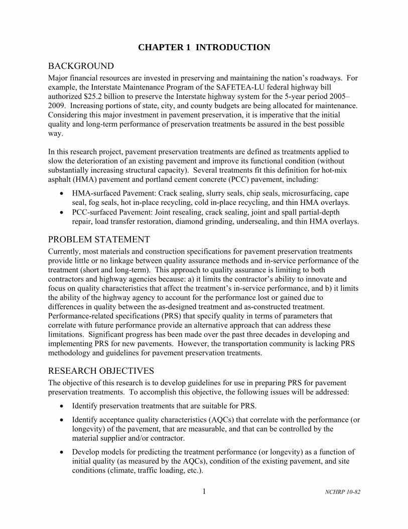
BACKGROUND Major financial resources are invested in preserving and maintaining the nation’s roadways. For example, the Interstate Maintenance Program of the SAFETEA-LU federal highway bill authorized $25.2 billion to preserve the Interstate highway system for the 5-year period 2005–2009. Increasing portions of state, city, and county budgets are being allocated for maintenance. Considering this major investment in pavement preservation, it is imperative that the initial quality and long-term performance of preservation treatments be assured in the best possible way. In this research project, pavement preservation treatments are defined as treatments applied to slow the deterioration of an existing pavement and improve its functional condition (without substantially increasing structural capacity). Several treatments fit this definition for hot-mix asphalt (HMA) pavement and portland cement concrete (PCC) pavement, including:

HMA-surfaced Pavement: Crack sealing, slurry seals, chip seals, microsurfacing, cape seal, fog seals, hot in-place recycling, cold in-place recycling, and thin HMA overlays.

PCC-surfaced Pavement: Joint resealing, crack sealing, joint and spall partial-depth repair, load transfer restoration, diamond grinding, undersealing, and thin HMA overlays.

PROBLEM STATEMENT Currently, most materials and construction specifications for pavement preservation treatments provide little or no linkage between quality assurance methods and in-service performance of the treatment (short and long-term). This approach to quality assurance is limiting to both contractors and highway agencies because: a) it limits the contractor’s ability to innovate and focus on quality characteristics that affect the treatment’s in-service performance, and b) it limits the ability of the highway agency to account for the performance lost or gained due to differences in quality between the as-designed treatment and as-constructed treatment. Performance-related specifications (PRS) that specify quality in terms of parameters that correlate with future performance provide an alternative approach that can address these limitations. Significant progress has been made over the past three decades in developing and implementing PRS for new pavements. However, the transportation community is lacking PRS methodology and guidelines for pavement preservation treatments.

RESEARCH OBJECTIVES The objective of this research is to develop guidelines for use in preparing PRS for pavement preservation treatments. To accomplish this objective, the following issues will be addressed:

Identify preservation treatments that are suitable for PRS.

Identify acceptance quality characteristics (AQCs) that correlate with the performance (or longevity) of the pavement, that are measurable, and that can be controlled by the material supplier and/or contractor.

Develop models for predicting the treatment performance (or longevity) as a function of initial quality (as measured by the AQCs), condition of the existing pavement, and site conditions (climate, traffic loading, etc.).

2 NCHRP 10-82

Develop a method for determining pay adjustment based on expenses or savings expected to occur in the future as a result of variation from the specified target level of quality.

Develop guidelines for establishing statistically sound sampling and testing acceptance plans.

Integrate the AQCs, acceptance sampling plans, performance/longevity prediction models, and pay adjustment methods into a coherent methodology and guidelines for developing PRS for pavement preservation treatments.

RESEARCH TASKS This research project is divided into two phases consisting of eight primary tasks, as follows:

Phase I (Tasks 1 through 4): This phase consists of the following four tasks: o Task 1— Review Literature and Current Practices. o Task 2— Develop a Process for Assessing the Suitability of Preservation

Treatments for PRS. o Task 3—Prepare a Detailed Outline of the Guidelines and a Plan for Developing

them in Phase II. o Task 4— Prepare Interim Report.

Phase II (Tasks 5 through 8): This phase involves the execution of the process for identifying preservation treatments suitable for PRS. A total of six preservation treatments deemed most suitable for PRS will be identified. The guidelines will be developed for these six treatments. Also, this phase includes the development of the guidelines and preparation of a final project report that documents the entire research effort. Phase II tasks are:

o Task 5— Identify Preservation Treatments for Consideration in the PRS Guidelines.

o Task 6—Develop PRS Guidelines and Methodology for Pavement Preservation Treatments.

o Task 7—Prepare Examples to Illustrate Use of the PRS Guidelines and Methodology.

o Task 8—Prepare Final Report. This report is the deliverable for Task 4, and it documents the research performed to date.

REPORT ORGANIZATION This report consists of six chapters. Chapter 1 (this chapter) presents the background of the research problem and describes the research objectives and scope. Chapter 2 presents key findings of a review of the literature on PRS and pavement preservation. Chapter 3 discusses current specifications for pavement preservation treatments (obtained from a sample of state DOTs). Chapter 4 presents a detailed outline of the PRS guidelines and a plan for developing them, taking into account all the knowledge gained in Phase I. Chapter 5 provides a systematic process for assessing the suitability of pavement preservation treatments for PRS based on the Analytic Hierarchy Process (AHP). Finally, Chapter 6 provides a closure to this report. The report includes four appendixes. Appendix A includes summary tables of current specifications for preservation treatments for HMA-surfaced and PCC-surfaced pavements. Appendix B provides a bibliography of existing performance prediction models for both HMA

3 NCHRP 10-82

and PCC pavements. Appendixes C and D contain site condition data for promising HMA and PCC treatment sections obtained from the Long-Term Pavement Performance (LTPP) database.

4 NCHRP 10-82

CHAPTER 2 LITERATURE REVIEW

This chapter presents key findings of the literature review regarding PRS and pavement preservation treatments.

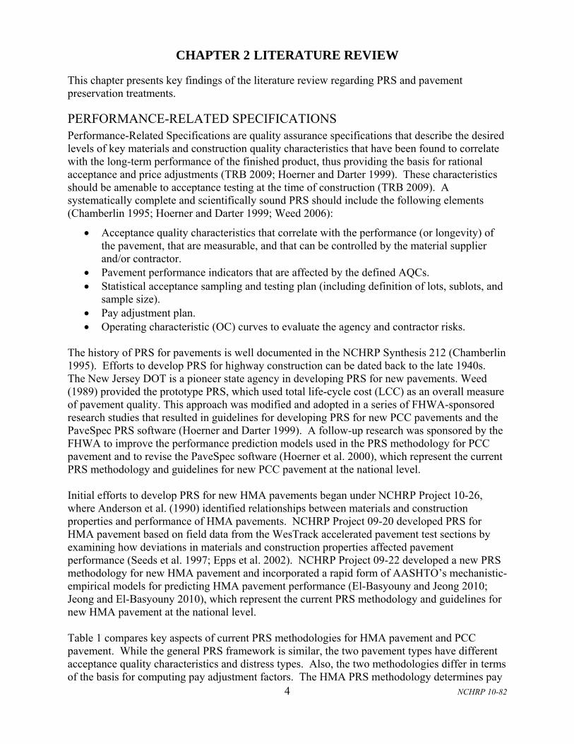
PERFORMANCE-RELATED SPECIFICATIONS Performance-Related Specifications are quality assurance specifications that describe the desired levels of key materials and construction quality characteristics that have been found to correlate with the long-term performance of the finished product, thus providing the basis for rational acceptance and price adjustments (TRB 2009; Hoerner and Darter 1999). These characteristics should be amenable to acceptance testing at the time of construction (TRB 2009). A systematically complete and scientifically sound PRS should include the following elements (Chamberlin 1995; Hoerner and Darter 1999; Weed 2006):

Acceptance quality characteristics that correlate with the performance (or longevity) of the pavement, that are measurable, and that can be controlled by the material supplier and/or contractor.

Pavement performance indicators that are affected by the defined AQCs. Statistical acceptance sampling and testing plan (including definition of lots, sublots, and

sample size). Pay adjustment plan. Operating characteristic (OC) curves to evaluate the agency and contractor risks.

The history of PRS for pavements is well documented in the NCHRP Synthesis 212 (Chamberlin 1995). Efforts to develop PRS for highway construction can be dated back to the late 1940s. The New Jersey DOT is a pioneer state agency in developing PRS for new pavements. Weed (1989) provided the prototype PRS, which used total life-cycle cost (LCC) as an overall measure of pavement quality. This approach was modified and adopted in a series of FHWA-sponsored research studies that resulted in guidelines for developing PRS for new PCC pavements and the PaveSpec PRS software (Hoerner and Darter 1999). A follow-up research was sponsored by the FHWA to improve the performance prediction models used in the PRS methodology for PCC pavement and to revise the PaveSpec software (Hoerner et al. 2000), which represent the current PRS methodology and guidelines for new PCC pavement at the national level. Initial efforts to develop PRS for new HMA pavements began under NCHRP Project 10-26, where Anderson et al. (1990) identified relationships between materials and construction properties and performance of HMA pavements. NCHRP Project 09-20 developed PRS for HMA pavement based on field data from the WesTrack accelerated pavement test sections by examining how deviations in materials and construction properties affected pavement performance (Seeds et al. 1997; Epps et al. 2002). NCHRP Project 09-22 developed a new PRS methodology for new HMA pavement and incorporated a rapid form of AASHTO’s mechanistic-empirical models for predicting HMA pavement performance (El-Basyouny and Jeong 2010; Jeong and El-Basyouny 2010), which represent the current PRS methodology and guidelines for new HMA pavement at the national level. Table 1 compares key aspects of current PRS methodologies for HMA pavement and PCC pavement. While the general PRS framework is similar, the two pavement types have different acceptance quality characteristics and distress types. Also, the two methodologies differ in terms of the basis for computing pay adjustment factors. The HMA PRS methodology determines pay

5 NCHRP 10-82

factors based on the difference in expected life between as-designed and as-constructed pavements; whereas, the PCC PRS methodology determines pay factors based on the difference in total LCC between as-designed and as-constructed pavements. Finally, the PCC PRS methodology considers both initial International Roughness Index (IRI) IRI (as an AQC) and is equipped with models to predict IRI (as a performance indicator); whereas the HMA PRS methodology considers pavement smoothness through user-defined pay adjustment factors for various values of initial IRI.

Table 1. Comparison of Current PRS Methodologies for New Pavements.

PRS Aspect New PCC Pavement New HMA Pavement

Acceptance Quality

Characteristics

PCC strength (compressive or flexural) Slab thickness Air content Initial smoothness (profile index or IRI) Consolidation around dowel bars

Asphalt concrete (AC) layer thickness Gradation: 3⁄4 in., 3⁄8 in., #4, and #200 Asphalt content (%) Gyratory mix air voids (%) Marshall mix air voids (%) In situ air voids from cores (%) Max. theoretical specific gravity of mix

(Gmm)

Predicted Performance

Transverse cracking Joint faulting Joint spalling International Roughness Index (IRI)

Bottom-up fatigue cracking Top-down (longitudinal) fatigue cracking Permanent deformation (rutting)

Pavement Smoothness

Initial smoothness is considered as an AQC

Future IRI is predicted as a performance indicator

User-defined pay factors based on initial IRI

Performance Prediction

Models

Empirical and Mechanistic-empirical models

Rapid closed-form of AASHTO’s mechanistic-empirical models

Basis for Pay Factor

Difference in life-cycle costs between as-designed and as-constructed pavements

Difference in expected lives between as-designed and as-constructed pavements

Composite Pay Factor

Individual pay factors combined using multiple options (multiplication, average, weighted average, etc.)

Overall pay factor computed based on LCC

Summation of individual pay factors

Currently, most materials and construction specifications for pavement preservation treatments provide little or no linkage between initial quality (material properties, construction quality, and design) and performance of the treatment (short and long-term). This approach to quality assurance is limiting to both contractors and highway agencies because: a) it limits the contractor’s ability to innovate and focus on quality characteristics that affect performance, and b) it limits the ability of the highway agency to account for the performance lost or gained due to differences between the as-designed product and as-constructed product. PRS that specify quality in terms of parameters that correlate with future performance provide an alternative approach that can address these limitations. This research effort will develop PRS methodology

6 NCHRP 10-82

and guidelines for pavement preservation treatments by building on the existing knowledge in PRS.

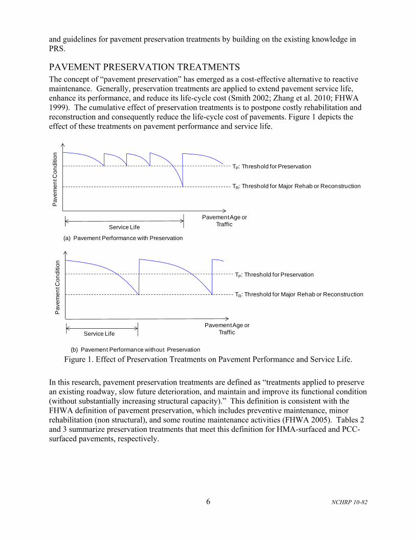
PAVEMENT PRESERVATION TREATMENTS The concept of “pavement preservation” has emerged as a cost-effective alternative to reactive maintenance. Generally, preservation treatments are applied to extend pavement service life, enhance its performance, and reduce its life-cycle cost (Smith 2002; Zhang et al. 2010; FHWA 1999). The cumulative effect of preservation treatments is to postpone costly rehabilitation and reconstruction and consequently reduce the life-cycle cost of pavements. Figure 1 depicts the effect of these treatments on pavement performance and service life.

Figure 1. Effect of Preservation Treatments on Pavement Performance and Service Life.

In this research, pavement preservation treatments are defined as “treatments applied to preserve an existing roadway, slow future deterioration, and maintain and improve its functional condition (without substantially increasing structural capacity).” This definition is consistent with the FHWA definition of pavement preservation, which includes preventive maintenance, minor rehabilitation (non structural), and some routine maintenance activities (FHWA 2005). Tables 2 and 3 summarize preservation treatments that meet this definition for HMA-surfaced and PCC-surfaced pavements, respectively.

Service Life

Pavement Age or Traffic

TR: Threshold for Major Rehab or Reconstruction

TP: Threshold for Preservation

Pa

vem

en

t Co

nd

itio

n

Service Life

Pavement Age or Traffic

Pa

vem

en

t Co

nd

itio

n

(a) Pavement Performance with Preservation

(b) Pavement Performance without Preservation

TR: Threshold for Major Rehab or Reconstruction

TP: Threshold for Preservation

7 NCHRP 10-82

Table 2. Preservation Treatments for HMA-Surfaced Pavements.

Treatment Description Purpose

Chip seals

Application of asphalt (typically an emulsion) to the pavement surface, followed by the application of rolled aggregate chips.

Seal longitudinal, transverse and block cracking

Inhibit and retard raveling/weathering (loose material must be removed)

Improve friction Reduce the intrusion of water into the

pavement Minor improvement to ride Inhibit low severity bleeding Inhibit moisture infiltration

Fog seals Very light application of a diluted asphalt emulsion placed directly on the pavement surface with no aggregate.

Seal fine low severity longitudinal, transverse, and block cracking

Enrich the hardened/oxidized asphalt Inhibit and retard raveling/weathering

Crack sealing Application of sealant (thermo-plastic bituminous materials) to “working” cracks that undergo little movement.

Prevent the intrusion of moisture through existing cracks

Slurry seals

A mixture of well-graded aggregate and asphalt emulsion spread in a thin layer (less than 0.4 in) over the entire pavement surface.


Retard asphalt aging, oxidation, and hardening

Inhibit low and medium severity bleeding Reduce the intrusion of water Minor improvement to ride Improve friction (especially at low speeds

(below 30 mph)

Microsurfacing

Application of a mixture of polymer-modified emulsified asphalt, mineral aggregate, mineral filler, water, and additives applied in a process similar to slurry seals.


Retard asphalt aging, oxidation, and hardening

Inhibit low and medium severity bleeding Improve friction (especially at low speeds Reduce the intrusion of water Improve surface friction A multiple course of microsurfacing is used

to correct pavement surface deficiencies, including rutting and minor surface profile irregularities

Thin HMA Overlay

Application of a thin layer of HMA.

Remove surface distresses Significantly improve ride (lower IRI) Seal pavement from surface water intrusion,

reduce transpiration of water upward through pavement

8 NCHRP 10-82

Table 2. Preservation Treatments for HMA-Surfaced Pavements (cont.).


Cold in-place recycling

Reclaimed asphalt pavement (without heat), combined with new emulsified or foamed asphalt and/or a rejuvenating agent, possibly also with virgin aggregate, and mixed at the pavement site to produce a new cold mix end product. Normally, cold in-place recycling is used in conjunction with an HMA overlay or chip seal.

Remove low-severity longitudinal, block, and transverse cracking

Remove raveling/weathering Improve friction Improve ride quality Inhibit low and medium severity bleeding

Hot in-place recycling

Softening the existing surface with heat, mechanically removing the pavement surface, mixing it with a recycling or rejuvenating agent, possibly adding virgin asphalt and/or aggregate, and replacing it on the pavement without removing the recycled material from the pavement site. Depth of treatment normally ranges between 0.75 and 2.0 in.

Remove low-severity longitudinal, block, and transverse cracking

Remove raveling/weathering Improve friction Improve ride quality Inhibit low and medium severity bleeding

Table 3. Preservation Treatments for PCC-Surfaced Pavements.


Diamond Grinding

Removal of a thin layer of PCC using stacked diamond tipped cutting blades

Remove faulting Improve surface rideability Improve surface friction

Load transfer restoration

Placement of load transfer devices (dowel bars) across joints or cracks in an existing pavement

Provide reliable load transfer Reduce or eliminate pumping, faulting,

and corner breaks (reducing deflections)

Partial-Depth Repair

Remove and replace relatively small deteriorated areas of PCC (usually < 10 sq. ft) and often only 2 to 3 in deep.

Repair shallow spalling associated with localized areas of scaling, weak concrete, clay balls, or high steel

Improve ride quality

Undersealing (or Slab

Stabilization)

Pressure insertion of flowable material beneath a PCC slab (ACPA 1994)

Fill underlying voids (not raise slab) Reduce pavement deflections Minimize pumping and faulting

Thin HMA Overlay

Application of a thin layer of HMA

Remove surface distresses Significantly improve ride (lower IRI) Seal pavement from surface water

intrusion, reduce transpiration of water upward through pavement

Joint Resealing

/Crack Sealing

Application of a sealant material in concrete pavement joints and cracks (ACPA 1993)

Minimize moisture infiltration Prevent intrusion of incompressibles

9 NCHRP 10-82

The literature contains very little hard data on the extent to which these treatments are used throughout the U.S. Much of the information in this regard is obtained through questionnaires, which can be influenced by the perception of the person who answered the questionnaire. Nonetheless, the results of these questionnaires provide indications of the treatment types that are being used nationwide. Key findings from the literature regarding the use of preservation treatments are summarized below:

A questionnaire survey of 13 state DOTs concerning HMA preservation treatments found that thin overlay (thickness less than 1.0 inch), microsurfacing (thickness less than 1.0 inch), crack sealing, and chip seal techniques are the most frequently used treatments for HMA-surfaced pavements (Morian 2011). The same survey indicated that chip seal is used primarily on low and medium volume roads (average daily traffic of 5,000 or less vehicles per day).

A study conducted under the Strategic Highway Research Program 2 (SHRP 2) Project R26 developed guidelines for selecting pavement preservation strategies specifically for high traffic volume roadways (Smith and Peshkin 2011). That study also included a questionnaire survey of highway agencies to identify what preservation treatments are used for high traffic volume roadways. Responses to the questionnaire from 50 highway agencies indicated that crack sealing, cold mill and HMA overlay, and drainage preservation are the most widely used HMA preservation treatments for high volume roads (average daily traffic of 10,000 or more vehicles per day). The same survey indicated that joint reseal, crack sealing, diamond grinding, and partial- and full-depth repairs are the most widely used PCC preservation treatments for high volume roads. The SHRP 2 study used sub-types of treatments. For example, the SHRP 2 study divides microsurfacing into single course and multi-course microsurfacing.

Montana DOT developed a synthesis of pavement maintenance and preservation through literature review and a web-based email survey that was distributed to all 50 U.S. states, Washington, D.C., and 11 Canadian provinces (Cuelho et al. 2006). Responses to the questionnaire from 34 U.S. states and five Canadian provinces indicated that crack sealing, thin overlays, chip seal, drainage features, and microsurfacing are the most frequently used treatments for HMA-surfaced pavements. The same survey indicated that diamond grinding and dowel bar retrofit are the most commonly used treatments for PCC-surfaced pavements. PCC partial- and full-depth repairs were not included in the Montana survey.

As part of NCHRP Project 14-14, Peshkin et al. (2004) identified pavement treatments that are used to preserve the system, retard future deterioration, and maintain and improve the functional condition of the system (without substantially increasing structural capacity). For HMA-surfaced pavements, these treatments included crack filling/crack sealing, fog seals, slurry seals, scrub seals, microsurfacing, chip seals, thin overlay, and ultrathin friction courses. For PCC-surfaced pavements, these treatments included joint/crack sealing, diamond grinding, undersealing, and load transfer restoration.

Although microsurfacing and slurry seal are listed separately in Table 2, NCHRP synthesis 411 found that most state DOT specifications include both microsurfacing and slurry seal together in the same specifications section, with little or no distinction between the two treatments (Gransberg 2010). Gransberg (2010) stated that the International Slurry Surfacing Association advocates categorizing both as “Slurry Systems” while maintaining the distinction that microsurfacing always contains a

10 NCHRP 10-82

polymer-modified emulsion that is designed to break chemically; thus allowing for opening the pavement for traffic within about an hour after application.

Some highway agencies include additional treatments (beyond those shown in Tables 2 and 3) in their preservation programs. For example, Michigan DOT includes full-depth repair in the preservation program for PCC-surfaced pavements (Galehouse 2002; Buch et al. 2003). Similarly, other highway agencies exclude some of the treatments shown in Tables 2 and 3 from their preservation programs. For example, Florida DOT does not use partial-depth repair for PCC-surfaced pavements.

CONSTRUCTION QUALITY AND IN-SERVICE PERFORMANCE OF ASPHALT PAVEMENT TREATMENTS The following sections provide discussions of the initial quality and in-service performance of primary treatments for HMA-surfaced pavements.

Chip Seal

A chip seal is a thin coat of asphalt (emulsion, modified or unmodified) followed by a thin layer of aggregate, placed on an existing pavement. Seal coat is the name usually used for this treatment when placed on a base course as part of a construction sequence. A chip seal, as the name implies, seals the underlying pavement from air and water intrusion and corrects and improves surface texture. As with other maintenance treatments, a chip seal has no significant structural impact and has little or no impact on rutting. Key quality indicators for chip seals include:

1. Air and pavement temperature within tolerance. 2. Clean surface, sealed cracks, and patched spot areas. 3. Proper quality, gradation, and quantity of aggregate. 4. Proper type, temperature, and application rate of asphalt binder. 5. Compatibility of binder and aggregate. 6. Construction timing (time between binder application and aggregate spread, time

between aggregate spread and rolling).

When placed properly, chip seals are an excellent, cost-effective treatment, especially for lower volume roads.

Slurry Seal and Microsurfacing

Slurry seal and mcrosurfacing consist of a thin (<3/8 inch) mixture of well-graded small sized aggregate (typically less than 1/4 inch), emulsified asphalt binder (and modifiers), squeegeed onto the pavement at ambient temperature. Microsurfacing uses a modified binder and mix design process and provides more stability; which is especially useful when the treatment is used to correct shallow rutting. Both treatments seal and protect the underlying surface, provide improved surface texture, and can improve ride quality. Slurry seals are often used in locations where high traffic volumes make chip seals problematic. Key quality indicators for slurry seals and microsurfacing include:

1. Clean surface, sealed cracks, and patched spot areas. 2. Proper quality and gradation of aggregate. 3. Proper type and percentage of asphalt binder and modifiers, if used. 4. Pavement temperature in the proper range. 5. Stockpile/plant/truck contamination.

11 NCHRP 10-82

6. Proper equipment calibration.

When slurry seals or microsurfacing are used on a cracked pavement, most cracks will reflect through fairly quickly. If the cracks in the existing pavement are wide (>3/8”), a wide crack, or even two cracks will develop, even if the cracks were sealed prior to the application. Some improved performance has been reported when cracks were filled with slurry material (instead of crack filler) prior to covering the surface.

Crack Sealing

Crack sealing is applied to keep air, water, and other foreign material from entering the pavement surface. Crack sealing is the least expensive preservation treatment. Typically, cracks are blown clean of debris with a jet of compressed air (sometimes heated air is used), and an asphaltic material, often with some type of rubber product, is applied at high temperature and squeegeed into the crack, forming a tight waterproof seal. Some agencies rout the crack prior to sealing. Cracks can be filled just below the surface, filled to the top of the surface, or overbanded where the crack is sealed and a thin layer (<1/16”) extends beyond the crack for approximately 1 inch on each side. Key quality indicators for crack sealing include:

1. Crack free of debris, clean, and dry. 2. Sealant heated to correct temperature. 3. If crack is heated, the pavement is not burnt. 4. Correct amount of material is applied in each crack.

Thin HMA Overlay

A thin hot-mix overlay is used when the pavement exhibits some functional problems. The overlay is too thin to address structural problems such as fatigue cracking or significant rutting. The situations where this treatment applies are to correct minor ride issues and skid resistance issues (flushing, polished aggregate). A thin overlay is used much like a seal coat or slurry seal, but is normally used on higher volume routes or as an alternative to these treatments. The most critical quality indicators for thin HMA overlays are:

1. Clean surface, sealed cracks, and patched spot areas. 2. Proper quality and gradation of aggregate. 3. Proper type and amount of asphalt binder. 4. Mix temperature at plant, mat temperature on pavement, and rolling temperatures

within tolerance. 5. Mat thickness.

HMA overlays have generally provided excellent service life and performance when placed properly on pavements without structural problems.

Cold-in-Place Recycling

Cold-in-place recycling is used to remove and replace the existing HMA pavement when there are problems with the existing surface, but the pavement structure is sound. In this treatment, the existing surface is milled, re-sized, and re-used; modifiers are added (including additional aggregate, emulsion, or some specialized asphalt product); and the pavement re-laid and compacted. A new surface course is usually added. This technique is the best option for surfaces that exhibit considerable cracking (non-fatigue related), aging, or even flushing of the asphalt surface. The mix design of the recycled pavement is very important. Some improvements to the existing profile can be realized and when the new surface is placed, the

12 NCHRP 10-82

roadway is nearly equivalent to a new road. The success of cold-in-place recycling is dependent on:

1. Control of milling depth and re-sizing operations. 2. Proper quality, gradation, and quantity of aggregate. 3. Accurate asphalt and modifier quantities. 4. Compaction operations and achieving target density. 5. Curing time prior to placing new surface and opening to traffic.

Hot-in-Place Recycling

Hot-in-place recycling is similar to cold-in-place in that it is used to remove and replace the existing HMA pavement when there are functional problems with the existing surface, but the pavement structure is sound. However, in this treatment the pavement surface is heated prior to milling, no cure time is required, and a new surface is not necessarily placed on top of the layer. Key quality indicators for hot-in-place recycling include:

1. Control of surface heating and milling depth. 2. Proper quality, gradation, and quantity of aggregate added. 3. Accurate asphalt and modifier quantities. 4. Compaction operations and achieving target density. 5. Surface profile control.

CONSTRUCTION QUALITY AND IN-SERVICE PERFORMANCE OF CONCRETE PAVEMENT TREATMENTS The following sections provide discussions of the initial quality and in-service performance of primary treatments for PCC-surfaced pavements.

Diamond Grinding

Rough and noisy patches, faulting, and bumps can be eliminated cost-effectively using diamond grinding. When patches are more than 10 per mile and faulting is more than 1/4 in., diamond grinding provides a smooth riding surface with good texture and reduces noise. When stabilized bumps or settled areas are present, diamond grinding can also be effective. Studies of ground pavement surfaces indicate that the depth of texture is strongly dependant on the age or the time since the grinding and indirectly on traffic since grinding. Climate also is a factor as where pavements in wet and dry freeze environments tend to have lower macro texture than those in the non-freeze regions. Ground sections in the wet and dry freeze environments regions would provide on the average 8 years of service life where those in the non-freeze regions provide 12 years of service life on the average. Key quality indicators for diamond grinding include:

1. Consistent transverse profile across the full width of the roadway. 2. Consistent longitudinal profile (particularly across transverse joints). 3. Smoothness. 4. Friction. 5. No adverse tracking issues (appropriate blade spacing and selection according to

aggregate hardness).

13 NCHRP 10-82

Load Transfer Restoration (Dowel Bar Retrofitting)

Load transfer restoration (also called dowel bar retrofitting) should be considered when faulting, high deflections, low load transfer efficiency ( LTE) of the joint/crack, or reflection cracks in the asphalt concrete overlay (ACOL) are detected. When LTE is lower than 70%, the basin area is less than 25 in., and joints are spalled more than 2 in. wide over more than 20% of the slabs, then restoration of load transfer is recommended. Pavements exhibiting material-related distresses such as D-cracking or reactive aggregate are not candidates for retrofit load transfer. Before and after restoring load transfer, slab stabilization may be needed to address loss of support and diamond grinding needed to remove the existing faulting. Key quality indicators for load transfer restoration include:

1. Placement and consolidation of the grout. 2. Alignment of the dowel. 3. Alignment and placement of the joint face restoration materials.

Load transfer retrofitting repairs have performed reasonably well, particularly where the grout material has stayed in place and has not prematurely spalled out.

Partial Depth Repair

The objective of partial depth repair is to repair spall distress without removing the entire slab. When 2 inch wide spalls are more than 10% of the crack or joint, partial depth repair is often employed using patching materials for PCC pavement or AC overlaid PCC pavement. The depth of spall should be less than 1/3 the thickness of the slab, and the pavement should have no reinforcing steel exposure. Partial depth repairs should restore the joint face, and the joint should be sealed properly. Key quality indicators for partial depth repairs include:

1. Method of curing. 2. Type of curing. 3. Weather conditions at the time of placing. 4. Strength of the bond at the existing concrete interface. 5. Moisture content and cleanliness of the surface concrete. 6. Drying shrinkage of the repair concrete.

Partial depth repairs have generally provided good service except where curing and bonding to the existing surface was inadequate and premature spalling of the repair shortens its effectiveness.

Slab Undersealing

Slab undersealing is used to restore uniform support by filling voids and reducing corner deflection, pumping, and faulting. Experienced contractors and proper inspection are essential to properly identify and underseal damaged areas, which is one of critical factors in effective undersealing operations. Therefore, Ground Penetrating Radar (GPR) is recommended to both locate and validate that voids have been properly identified and filled. Slab undersealing is recommended when GPR-indicated voided cracks or joints are more than 20% of the inspected section or where unstable bumps or unstable settlement is present. The success of undersealing is strongly connected to the adequacy of the void filling; many undersealed projects have failed to provide adequate service due to eradicate void filling or filling non-voided areas resulting in uneven or non-supported slabs.

14 NCHRP 10-82

Thin ACOL

A thin AC overlay with petromat can be used to restore the functional capacity of a pavement and improve rideability. Employing a thin AC overlay for hard aggregate pavements may be a good alternative to diamond grinding.

Existing structural distresses must be repaired and restored before the overlay is placed. This is important particularly if the pavement is structurally deficient to avoid premature failure. Use of a crack attenuating mix with good aggregate is recommended to minimize reflection cracking. Key quality indicators for thin ACOLs include:

1. Existing condition and roughness – amounts and type of cracking. 2. Control of gradation. 3. Temperature of placement. 4. AC content. 5. Compaction.

Routinely, thin ACOLs provide about 5 to 10 years of service life, depending on the above factors until additional faulting and spalling occur in the pavement.

Joint Resealing and Crack Sealing

Crack sealing is recommended when crack width is wider than 0.03 inch. Resealing joints and cracks is recommended when sealants are damaged over more than 20% along the joint or crack to reduce infiltration of moisture and incompressible material over time. Service life for sealants can be anywhere from 7 to 10 years, performance can be short lived if water is not cleared from the joint prior to placement of the seal. Water trapped by the sealing operation can rapidly deteriorate the bond between the seal and the face of the joint. Thus, trapped subsurface water should be removed before re-sealing operations. Selection of proper sealing material should be based on temperature and moisture conditions. Key quality indicators for joint and crack sealing/resealing include:

1. Moisture in the existing concrete. 2. Clean and dry joint face. 3. Backer rod positioning. 4. Hot applied placement temperature and minimizing over-banding. 5. Removing water from the joint and its vicinity.

15 NCHRP 10-82

CHAPTER 3 CURRENT SPECIFICATIONS FOR PAVEMENT PRESERVATION TREATMENTS

This chapter provides an overview of current specifications for pavement preservation treatments.

AVAILABILITY OF SPECIFICATIONS Table 4 shows the availability of materials and construction specifications for most commonly-used pavement preservation treatments in a sample of 14 state DOTs. These agencies were selected to provide a broad geographic distribution throughout the United States. It can be seen that most of these agencies have developed specifications for pavement preservation treatments. While these specifications are predominantly method-based, they provide clues of acceptance quality characteristics that can be measured during or immediately after construction. Samples of these specifications were reviewed and summarized. Table 5 lists the specifications reviewed and summarized in this study. A discussion of these specifications is presented in the following section of this report. Appendix A provides the summary tables. Table 4. Availability of Specifications for Commonly-Used Preservation Treatments at Sample

State DOTs.

State DOT

PCC-surfaced Treatments* HMA-surfaced Treatments*

PDR FDR DG LTR JR US CS SS CrS CIR HIR TOL AZ CA FL IA ID KS MI MT NC NY PA SD TX WA

*PDR=Partial-Depth Repair; FDR=Full-Depth Repair; DG=Diamond Grinding; LTR=Load Transfer Restoration; JR=Joint Resealing; US=Undersealing; CS=Chip Seals; SS=Slurry Seal or Microsurfacing; CrS= Crack Sealing; CIR=Cold in-place recycling; HIR=Hot in-place recycling; TOL=Thin HMA Overlay.

The following discussions focus on the materials and construction quality measures used in the reviewed specifications. This review will help identify acceptance quality characteristics that can potentially be used in the PRS guidelines (to be developed later in Phase II of this research project). Additional relevant aspects of the specifications, such as pay adjustment, are also discussed.

16 NCHRP 10-82

Table 5. Specifications Discussed and Summarized in This Report (See Appendix A).

State DOT

PCC-surfaced Treatments HMA-surfaced Treatments

PDR FDR DG LTR JR US CS SS CrS CIR HIR TOL AZ

CA FL

IA

ID

KS MI

MT

NC

NY

PA

SD

TX WA

CURRENT SPECIFICATIONS FOR HMA-SURFACED PAVEMENT TREATMENTS

Chip Seal

Most of the 14 state DOTs included in this review have standard specifications for chip seals. Some DOTs have multiple specifications for chip seals, depending on the type of material used, and number of layers. Material quality measures include testing of asphalt materials and aggregate. Construction quality measures include application rate of aggregate and asphalt material, and number of roller passes. The most common construction quality measures are the application rates of asphalt and aggregate. Few states have pay adjustment in their specifications based on construction quality. Some DOTs (such as Montana, Michigan, and California DOTs) have a form of warranty for chip seals.

Slurry Seal

Only five of the 14 state DOTs included in this review have separate specifications for slurry seals. Common materials quality measures include testing of asphalt emulsion (generally SS-1h and CSS-1h), fine aggregate and filler (if used), asphalt cement content, and gradation of aggregate. Construction quality measures include slurry spread rate and mix consistency.

Crack Sealing

Ten of the 14 state DOTs included in this review have separate specifications for crack sealing. Materials quality measures refer to the testing of crack sealant materials. Only one state requires the testing of backer rod in their specifications. Construction quality measures include depth of crack cleaned, adhesion and cohesion failure, and missed cracks.

Thin HMA Overlay

Thin HMA overlay treatment refers to plant-mixed asphalt binder and aggregate applied to existing HMA pavement as an overlay with thicknesses typically 1.0 inch, or less and that does

17 NCHRP 10-82

not significantly add structural strength to the pavement. Only a few state DOTs have separate specifications specific for this treatment. Most state DOTs include this treatment in their specification for HMA pavement, stone mastic asphalt, open graded friction course, etc. with or without minor modifications. Whereas the same table contains the guide specification for the ultra-thin HMA overlay from Michigan. Typically the construction and materials quality of this treatment include asphalt content, percent passing of aggregate for certain sieve sizes, in-place and laboratory density, and smoothness. State DOTs apply varying pay adjustment schemes (different adjustments for different AQCs).

Cold-in-Place Recycling

Only six of the 14 state DOTs included in this review have separate specifications for cold-in-place recycling. Three states have special specifications and the other two have standard specifications. Materials quality measures include the testing of asphaltic material added as recycling agent or rejuvenator, and the testing of aggregate quality if any additional aggregate is added during the recycling process. Size of pulverizing of existing surface course is one of the construction quality measures. Generally the maximum size allowable during the pulverization ranges from 1 to 2 inches. Other construction related quality measures include smoothness, depth of planning of surface course, and application rate of bituminous materials (recycling agent).

Hot-in-Place Recycling

Only four of the 14 state DOTs included in this review have separate specifications for hot-in-place recycling. Materials quality measures include testing of asphalt materials used as recycling agent and asphalt from existing surface course, quality of virgin HMA (if used). Construction quality measures include smoothness of finished surface, depth of scarification of existing surface course, percentage of recycling agent, percentage of virgin HMA (if used), and placement of construction joint.

CURRENT SPECIFICATIONS FOR PCC-SURFACED PAVEMENT TREATMENTS

Diamond Grinding

Most of the 14 state DOTs included in this review have standard specifications for diamond grinding. Typically, construction quality measures include smoothness, percentage of ground area, height of individual bump, and groove dimensions. California and Arizona also require certain amount of coefficient of friction on ground surface. Smoothness of treated surface is evaluated by measuring profile index or the IRI. Half of the reviewed specifications have a pay adjustment scheme based on the smoothness of treated surface.

Full-Depth Repair

Majority of the 14 state DOTs included in this review have standard specifications for full-depth repair treatment. These specifications have mixed definitions of full-depth repair, depending on the width of patching. The acceptance quality characteristics include smoothness, location of dowel and tie bars, and compressive strength of concrete. Some states have pay adjustment factors based on concrete strength and depth of patching.


Ten of the 14 state DOTs included in this review have standard specifications for concrete pavement partial-depth repair. The patching materials consist of different types of cement concrete, epoxy resin, cement grout, and HMA. Typically the DOTs specify several laboratory

18 NCHRP 10-82

tests as acceptance criteria for the patching materials. The most common construction quality measure among the reviewed specifications is the depth of saw cutting. Other construction related quality measures include testing of smoothness and sounding. None of the reviewed specifications has a quality-based pay adjustment.

Joint Resealing and Crack Sealing

Ten of the 14 state DOTs included in this review have standard specifications for joint resealing and crack sealing (both transverse and longitudinal cracks). Materials quality measures of joint and crack sealing mainly consist of testing of sealants. Generally, states accept silicone joint sealant or asphalt rubber sealant.

Load Transfer Restoration

Nine of the 14 state DOTs included in this review have standard specifications for dowel bar retrofitting to restore load transfer efficiency. Materials quality measures primarily consist of testing of dowel bar and patching materials. Patching material includes cement concrete, epoxy resin, and grout. Most of states verify the positing of dowel bar as a construction quality measure. Other construction quality is verified for the compressive strength of patching material, and saw cut depth. South Dakota DOT’s specifications include a pay reduction if the 24-hour concrete strength does not meet the minimum 4000 psi requirement.

Slab Stabilization (Undersealing)

Seven of the 14 state DOTs included in this review have standard or special specifications for slab stabilization or undersealing of PCC pavement. The grout quality measures include testing such as efflux time, set time, compressive strength, and volume expansion property. Construction quality measures include maximum amount of upward movement of the slab, deflection of slab, and smoothness. South Dakota and Iowa DOTs apply pay reduction if any radial cracking develops during grouting.

19 NCHRP 10-82

CHAPTER 4 OUTLINE AND DEVELOPMENT PLAN FOR PRS GUIDELINES

This chapter presents a detailed outline of the PRS guidelines and a plan for developing them.

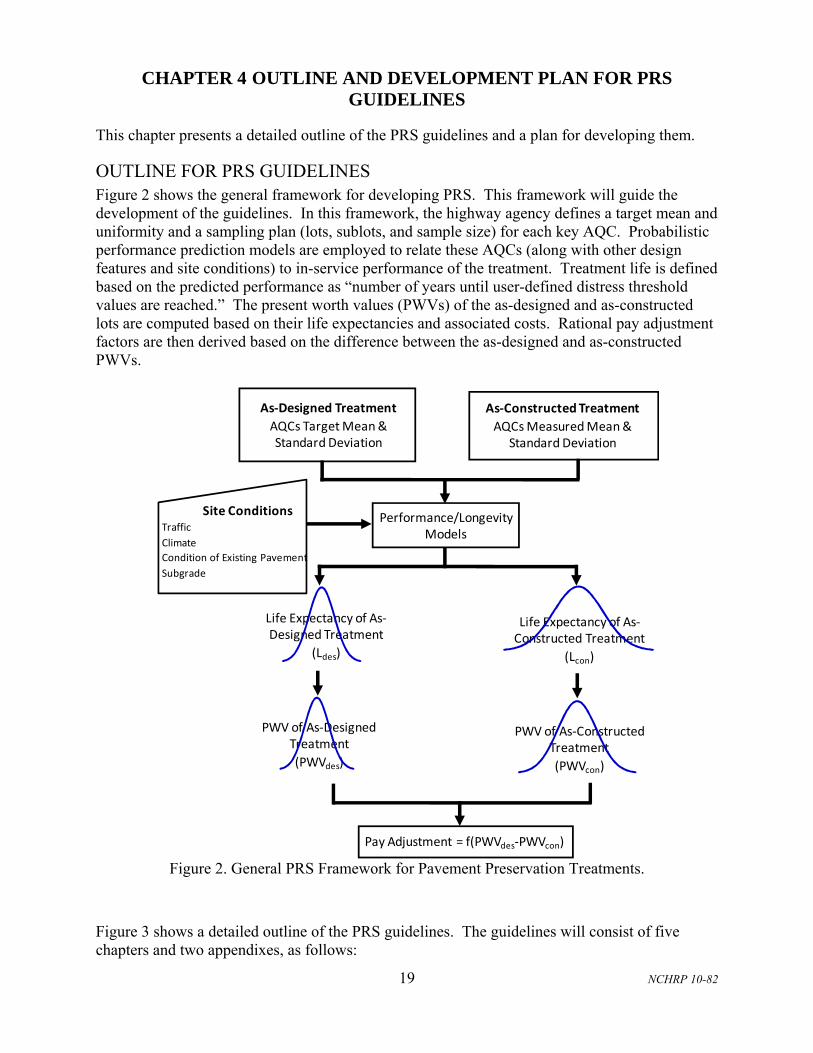
OUTLINE FOR PRS GUIDELINES Figure 2 shows the general framework for developing PRS. This framework will guide the development of the guidelines. In this framework, the highway agency defines a target mean and uniformity and a sampling plan (lots, sublots, and sample size) for each key AQC. Probabilistic performance prediction models are employed to relate these AQCs (along with other design features and site conditions) to in-service performance of the treatment. Treatment life is defined based on the predicted performance as “number of years until user-defined distress threshold values are reached.” The present worth values (PWVs) of the as-designed and as-constructed lots are computed based on their life expectancies and associated costs. Rational pay adjustment factors are then derived based on the difference between the as-designed and as-constructed PWVs.

Figure 2. General PRS Framework for Pavement Preservation Treatments.

Figure 3 shows a detailed outline of the PRS guidelines. The guidelines will consist of five chapters and two appendixes, as follows:

Performance/Longevity Models

Life Expectancy of As‐Designed Treatment

(Ldes)

Site ConditionsTraffic

Climate

Condition of Existing Pavement

Subgrade

As‐Designed Treatment

AQCs Target Mean & Standard Deviation

As‐Constructed Treatment

AQCsMeasured Mean & Standard Deviation

Life Expectancy of As‐Constructed Treatment

(Lcon)

Pay Adjustment = f(PWVdes‐PWVcon)

PWV of As‐Designed Treatment

(PWVdes)

PWV of As‐Constructed Treatment

(PWVcon)

20 NCHRP 10-82

Chapter 1 – Introduction: This chapter begins with introducing the primary concepts of both pavement preservation and PRS. Then, it defines the purpose and scope of the guidelines, including identifying treatments that are found to be most suitable for PRS (three treatments for HMA-surfaced pavement and three treatments for PCC-surfaced pavements). Finally, this chapter describes how to use the guidelines to generate PRS.

Chapter 2 –PRS Methodology for Pavement Preservation Treatments: This chapter defines the components and flow of the PRS methodology, including inputs and outputs.

Chapter 3 – Guidelines for Determining Acceptance Quality Characteristics for Preservation Treatments: This chapter identifies key construction and materials acceptance quality characteristics for each treatment deemed suitable for PRS (a total of six treatments). Additionally, this chapter describes testing and measurement methods available for these AQCs. Finally, it provides guidance on selecting appropriate mean and variability target values for each AQC.

Chapter 4 – Guidelines for Developing Statistical Acceptance Sampling Plans: This chapter will provide guidelines for developing and evaluating acceptance sampling plans for use in PRS. The guidelines will address issues related to defining lots, sublots, and sample size, and developing operating characteristic curves that assess the agency’s and contractor’s risks.

Chapter 5 – Guidelines for Applying PRS: This chapter provides guidance on how to prepare PRS prior to letting preservation projects and how to apply PRS in the field (including implementing sampling plans and pay adjustment schemes).

Appendix A – Illustrative Examples of PRS Development: These examples will be designed to illustrate the use of the PRS guidelines for different preservation treatments (six treatments found most suitable for PRS), pavement types (HMA-surfaced pavement and PCC-surfaced pavement), highway classification (high, medium, and low traffic volumes), and climatic regions.

Appendix B –Performance Prediction Models for Preservation Treatments: Performance prediction models are vital for developing PRS. They provide a necessary link between initial quality and in-service performance. This appendix will describe the developed models, define their inputs and outputs, and assess their sensitivity to key inputs.

21 NCHRP 10-82

Figure 3. Outline for the Guidelines for Preparing PRS for Pavement Preservation Treatments.

Chapter 1 – Introduction 1.1 Background on PRS and Pavement Preservation 1.2 Purpose of Guidelines 1.3 Scope of the Guidelines (Treatments Suitable for PRS) 1.3.1 HMA-surfaced Pavement Preservation Treatments 1.3.2 PCC-surfaced Pavement Preservation Treatments 1.4 How to Use the Guidelines

Chapter 2 – PRS Methodology for Pavement Preservation Treatments

2.1 Description of PRS Methodology 2.2 Predicting Treatment Performance

2.2.1 HMA-surfaced Pavement Preservation Treatments 2.2.2 PCC-surfaced Pavement Preservation Treatments

2.3 Life Cycle Cost as an Overall Measure of Treatment Quality 2.3.1 Agency Costs

2.3.2 User Costs (if found suitable for PRS) 3.4 Development of Pay Factor Curves

Chapter 3 – Guidelines for Determining Acceptance Quality Characteristics (AQCs) for Preservation Treatments

3.1 HMA-surfaced Pavement Preservation Treatments 3.1.1 Key AQCs 3.1.2 Testing and Measurement Methods for AQCs 3.1.3 Determining Target Values for AQCs (mean and variability)

3.2 PCC-surfaced Pavement Preservation Treatments 3.2.1 Key AQCs 3.2.2 Testing and Measurement Methods for AQCs 3.2.3 Determining Target Values for AQCs (mean and variability)

Chapter 4 – Guidelines for Developing Statistical Acceptance Sampling Plans

4.1 Defining Lots and Sublots 4.2 Determining Sample Size 4.3 Defining Acceptable and Rejectable Quality Levels 4.4 Assessing Agency’s and Contractor’s Risks

Chapter 5 – Guidelines for Applying PRS

5.1 Preparation of PRS Prior to Project Letting 5.2 Applying PRS in the Field

Appendix A – Illustrative Examples of PRS Development 1. Examples for HMA-surfaced Pavement Preservation Treatments 2. Examples for PCC-surfaced Pavement Preservation Treatments Appendix B – Performance Prediction Models for Preservation Treatments 1. Models for HMA-surfaced Pavement Preservation Treatments 2. Models for PCC-surfaced Pavement Preservation Treatments

22 NCHRP 10-82

PLAN FOR DEVELOPING PRS GUIDELINES The following sections describe the steps that will be taken in Phase II of the project to develop the PRS guidelines.

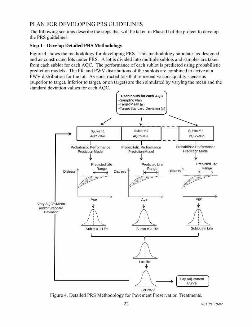
Step 1 - Develop Detailed PRS Methodology

Figure 4 shows the methodology for developing PRS. This methodology simulates as-designed and as-constructed lots under PRS. A lot is divided into multiple sublots and samples are taken from each sublot for each AQC. The performance of each sublot is predicted using probabilistic prediction models. The life and PWV distributions of the sublots are combined to arrive at a PWV distribution for the lot. As-constructed lots that represent various quality scenarios (superior to target, inferior to target, or on target) are then simulated by varying the mean and the standard deviation values for each AQC.

Figure 4. Detailed PRS Methodology for Pavement Preservation Treatments.

Sublot # 1 Sublot # 2 Sublot # n

AQC Value

Lot Life

Lot PWV

User Inputs for each AQC•Sampling Plan•Target Mean ()•Target Standard Deviation ()

Probabilistic Performance Prediction Model

Sublot # n Life

Age

Distress

Predicted Life Range

AQC ValueAQC Value


Sublot # 2 Life

Age

Distress



Sublot # 1 Life

Age

Distress


Vary AQC’s Mean and/or Standard

Deviation

Pay Adjustment Curve

23 NCHRP 10-82

Pay factor (PF) is determined for each AQC based on the expected saving (or loss) to the agency throughout an agency-specified life cycle period, as follows:

100

d cPWV PWV PPF

Bid

(4-1)

where PF = pay factor as a percentage of bid price, % dPWV = present-worth value of as-designed lot at confidence level

cPWV = present-worth value of as-constructed at confidence level

P = probability of PWV between dPWV and cPWV

Bid = bid price, $ The above formula is best explained through possible quality scenarios, as follows:

Equal Quality: If the as-constructed lot has mean and standard deviation values equal to those specified by the agency as targets, the as-constructed and as-designed PWV distribution curves will be identical and thus the contractor receives full payment (i.e., PF = 100%).

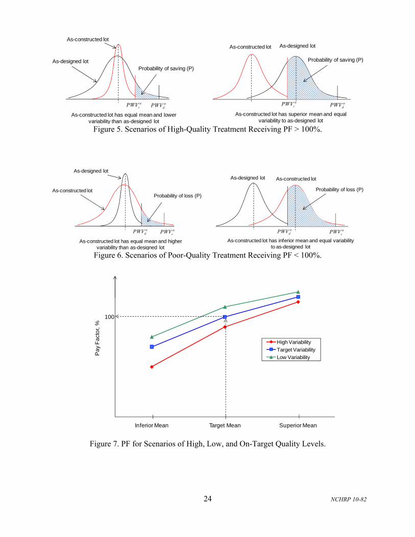
High Quality: If the as-constructed lot has higher quality than the as-designed lot (i.e., as-constructed mean and/or standard deviation values of the AQC are superior to the agency-specified targets), the as-constructed PWV distribution curve will be shifted to the left of the as-designed PWV distribution curve; and thus the contractor receives a pay increase (i.e., PF > 100%). Figure 5 shows this scenario graphically.

Poor Quality: If the as-constructed lot has lower quality than the as-designed lot (i.e., as-constructed mean and/or standard deviation values of the AQC are inferior to the agency-specified targets), the as-constructed PWV distribution curve will be shifted to the right of the as-designed PWV distribution curve; and thus the contractor receives a pay reduction (i.e., PF < 100%). Figure 6 depicts this scenario graphically.

Figure 7 shows typical PF curves for the above scenarios of quality. The lot composite (overall) pay factor is normally computed as the multiplication or weighted average of the individual pay factors. State DOTs can assign minimum and maximum limits on composite pay factors for practical reasons. For example, the minimum limit can be 90% and the maximum limit 110% of the bid price, representing a 10% maximum incentive or disincentive.

24 NCHRP 10-82

Figure 5. Scenarios of High-Quality Treatment Receiving PF > 100%.

Figure 6. Scenarios of Poor-Quality Treatment Receiving PF < 100%.

Figure 7. PF for Scenarios of High, Low, and On-Target Quality Levels.

cPWV dPWV

As-constructed lot As-designed lot

As-constructed lot has superior mean and equal variability to as-designed lot

cPWV dPWV

As-constructed lot has equal mean and lower variability than as-designed lot

As-constructed lot

As-designed lotProbability of saving (P)

Probability of saving (P)

cPWV dPWV

As-constructed lotAs-designed lot

As-constructed lot has inferior mean and equal variability to as-designed lot

cPWV dPWV

Probability of loss (P)

As-constructed lot has equal mean and higher variability than as-designed lot

As-constructed lot

As-designed lot

Probability of loss (P)

Inferior Mean Target Mean Superior Mean

Pa

y F

act

or,

%

High Variability

Target Variability

Low Variability

100

25 NCHRP 10-82

Step 2 – Identify Acceptance Quality Characteristics and Performance Indicators for Selected Pavement Preservation Treatments

AQCs and performance indicators are core elements of PRS. The essence of PRS is that these two elements can be linked through mathematical relationships. As mentioned earlier, AQCs that are amenable to PRS can be described as follows:

Measurable at the time of construction. Can be controlled by the contractor or material supplier. Affect the future performance of the preservation treatments.

As discussed in the previous chapter, the availability of these AQCs is a key factor in determining the suitability of treatments for PRS. Existing specifications (summarized in Chapter 2) and existing databases (e.g., the LTPP database) will be used to determine the availability of AQCs for each treatment. Also, existing laboratory and field testing procedures will be evaluated to determine their suitability for measuring AQCs for the selected treatments. Potential AQCs for various pavement preservation treatments have been identified based on SHRP studies SHRP-H-358 and SHRP-M/FR-92-102 (Smith et al. 1993; Bullard et al. 1992). These potential AQCs for HMA-surfaced and PCC-surfaced pavement treatments are listed as follows:

HMAC-surfaced Pavement (both flexible and composite pavements).

o Binder/bituminous material application rate. o Binder/bituminous material application temperature. o Aggregate application rate. o Mineral filler application rate (slurry seal). o Percent of cracks sealed. o Aggregate maximum size. o Aggregate gradation. o Aggregate physical properties (cleanliness, shape, toughness, and absorption). o Time between application of bituminous material and spreading of aggregate. o Number of coverages per roller. o Time between final rolling and opening to traffic. o Sealant temperature (crack sealing only). o Time between crack sealing and opening to traffic (crack sealing only). o Initial Smoothness (e.g., International Roughness Index, IRI).

PCC-surfaced Pavement.

o Sealant properties (temperature, width, and depth below pavement surface) (crack sealing and joint resealing).

o Width of crack or joint (crack sealing and joint resealing). o Depth of backer rod (joint resealing). o Sealant application pressure (crack sealing and joint resealing). o Area of removed deteriorated concrete (partial-depth repair). o Time of setting of repair material (partial-depth repair, dowel bar retrofitting). o Strength of repair material (compressive or flexural) (partial-depth repair). o Porosity of repair material. o Fracture roughness of repair material.

26 NCHRP 10-82

o Bond shear strength between base concrete and spall repair material (partial-depth repair).

o Consolidation of repair material. o Compatibility in thermal expansion between the repair material and the original

PCC slab (partial-depth repair). o Initial surface texture (e.g., sand patch test) (diamond grinding). o Groove characteristics (height, groove, land area, and number of grooves per ft). o Initial smoothness (e.g., IRI).

The final set of AQCs for the selected six treatments (three treatments for HMA-surfaced pavement and three treatments for PCC-surfaced pavements) will be determined in Subtask 5.2 (Identify Existing Laboratory and Field Tests for the Selected Treatments) of Phase II. Current state DOTs specifications for pavement preservation treatments provide additional guidance for selecting AQCs that are suitable for PRS and at the same time practical to implement (see the next chapter of this report). Once the AQCs are identified, performance indicators (individual distress type, overall condition indexes, or roughness indexes) that can be linked to these AQCs will be identified. There are dozens of types of distress types and conditions indexes for both HMA and PCC pavements (Huang 2004). Not all of them can be used in PRS for pavement preservation treatments. For preservation treatments, the selection of performance indicators should be done with great caution because each preservation treatment is intended to address very few distress types in the existing pavement. For example, chip seal is intended to address skid resistance, polishing, and a limited amount of cracking. It should not be expected to address rutting, roughness, and high-severity cracking.

Step 3 - Develop Performance Prediction Models for Pavement Preservation Treatments

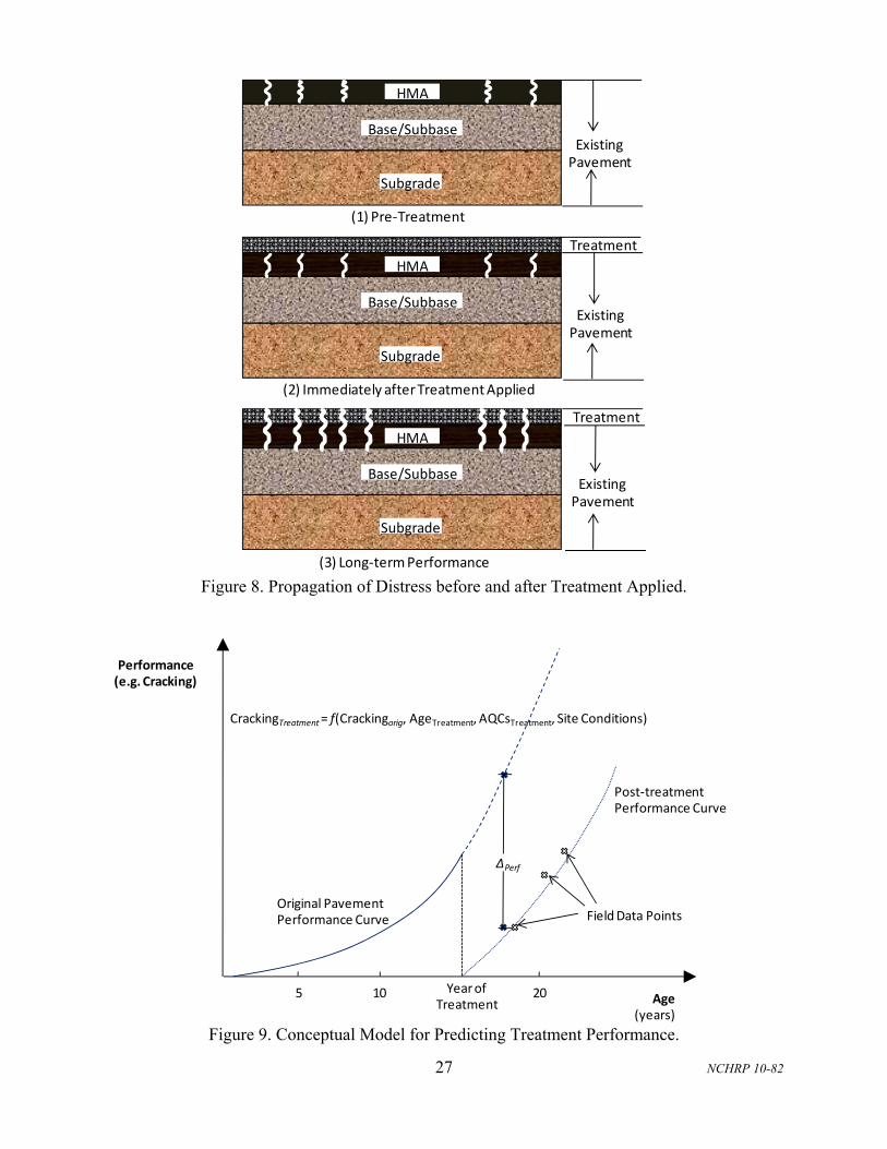
Performance prediction models are crucial components of PRS. Through these models, the material and construction quality of the treatments (as measured by key AQCs) is related to the in-service performance and life-cycle costs of the treatment. As discussed earlier, the ability to relate AQCs (measured during or immediately after construction) to in-service performance allows for developing rational pay adjustment schemes. Since, by definition, preservation treatments do not substantially increase the structural capacity to the existing pavement, their performance is affected by both their AQCs and the condition of the original (existing) pavement. For example, the structural layers underneath the treatment govern the initiation and propagation of cracking into the treatment, as illustrated in Figure 8. Figure 9 displays a conceptual model for predicting treatment performance as a function of condition of the existing pavement, AQCs of treatment, age of treatment, and site conditions (traffic loading, climate, etc.). This concept requires the use of reliable models for predicting the condition of the existing pavement and the availability of field performance data for the preservation treatments. Existing models will be used for predicting the condition of the original pavement. The literature is rich in these models for both HMA and PCC pavements. However, these existing models vary in terms of their type (mechanistic, empirical, or mechanistic-empirical), predicted performance indicators and distress type, and suitability for PRS. Appendix B provides a bibliography of these models. Field performance data for the selected preservation treatments will be obtained from existing databases (such as the LTPP database).

27 NCHRP 10-82

Figure 8. Propagation of Distress before and after Treatment Applied.

Figure 9. Conceptual Model for Predicting Treatment Performance.

Subgrade

Base/Subbase

HMA

(1) Pre‐Treatment

(2) Immediately after Treatment Applied

Subgrade

Base/Subbase

HMA

Treatment

(3) Long‐term Performance

Subgrade

Base/Subbase

HMA

Existing Pavement

Existing Pavement

Treatment

Existing Pavement

Age(years)

Performance (e.g. Cracking)

5 10 20

CrackingTreatment= f(Crackingorig, AgeTreatment, AQCsTreatment, Site Conditions)

Year of Treatment

Post‐treatment Performance Curve

Original Pavement Performance Curve

ΔPerf

Field Data Points

28 NCHRP 10-82

Example Performance Prediction Models

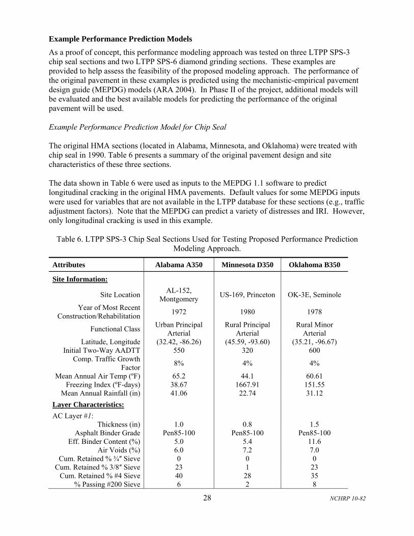
As a proof of concept, this performance modeling approach was tested on three LTPP SPS-3 chip seal sections and two LTPP SPS-6 diamond grinding sections. These examples are provided to help assess the feasibility of the proposed modeling approach. The performance of the original pavement in these examples is predicted using the mechanistic-empirical pavement design guide (MEPDG) models (ARA 2004). In Phase II of the project, additional models will be evaluated and the best available models for predicting the performance of the original pavement will be used. Example Performance Prediction Model for Chip Seal The original HMA sections (located in Alabama, Minnesota, and Oklahoma) were treated with chip seal in 1990. Table 6 presents a summary of the original pavement design and site characteristics of these three sections. The data shown in Table 6 were used as inputs to the MEPDG 1.1 software to predict longitudinal cracking in the original HMA pavements. Default values for some MEPDG inputs were used for variables that are not available in the LTPP database for these sections (e.g., traffic adjustment factors). Note that the MEPDG can predict a variety of distresses and IRI. However, only longitudinal cracking is used in this example.

Table 6. LTPP SPS-3 Chip Seal Sections Used for Testing Proposed Performance Prediction Modeling Approach.

Attributes Alabama A350 Minnesota D350 Oklahoma B350

Site Information:

Site Location AL-152,

Montgomery US-169, Princeton OK-3E, Seminole

Year of Most Recent Construction/Rehabilitation

1972 1980 1978

Functional Class Urban Principal

Arterial Rural Principal

Arterial Rural Minor

Arterial Latitude, Longitude (32.42, -86.26) (45.59, -93.60) (35.21, -96.67)

Initial Two-Way AADTT 550 320 600 Comp. Traffic Growth

Factor 8% 4% 4%

Mean Annual Air Temp (ºF) 65.2 44.1 60.61 Freezing Index (ºF-days) 38.67 1667.91 151.55

Mean Annual Rainfall (in) 41.06 22.74 31.12

Layer Characteristics:

AC Layer #1: Thickness (in) 1.0 0.8 1.5

Asphalt Binder Grade Pen85-100 Pen85-100 Pen85-100 Eff. Binder Content (%) 5.0 5.4 11.6

Air Voids (%) 6.0 7.2 7.0 Cum. Retained % ¾ʺ Sieve 0 0 0

Cum. Retained % 3/8ʺ Sieve 23 1 23 Cum. Retained % #4 Sieve 40 28 35

% Passing #200 Sieve 6 2 8

29 NCHRP 10-82


AC Layer #2:

Thickness (in) 3.0 4.0 8.8 Asphalt Binder Grade Pen85-100 Pen120-150 Pen85-100

Eff. Binder Content (%) 5.0 7.0 11.0 Air Voids (%) 6.0 4.0 3.7

Cum. Retained % ¾ʺ Sieve 10 0 20 Cum. Retained % 3/8ʺ Sieve 34 18 50

Cum. Retained % #4 Sieve 42 40 57 % Passing #200 Sieve 2 4 6

AC Layer #3:

Thickness (in) 6.5 - - Asphalt Binder Grade Pen85-100 - -

Eff. Binder Content (%) 5.0 - - Air Voids (%) 8.0 - -

Cum. Retained % ¾ʺ Sieve 14 - - Cum. Retained % 3/8ʺ Sieve 36 - -

Cum. Retained % #4 Sieve 54 - - % Passing #200 Sieve 1 - -

Base/Subbase:

Material Type Soil-aggregate

mixture A-1-b A-1-a

Thickness (in) 6.0 6.0 12.0 Modulus (input) (psi) 10,000 38,000 29,500

Plasticity Index 1 1 0 Liquid Limit 6 11 6

% Passing #200 Sieve 8.7 6.9 12 % Passing #4 Sieve 44.7 63 41

Subgrade:

AASHTO Soil Class A-7-6 A-2-4 A-1-a CBR (%) 9 - -

Modulus (psi) 10,426 (calculated) 30,000 (input) 29,500 (input) Plasticity Index 17 2 0

Liquid Limit 47 14 6 % Passing #200 Sieve 76.6 14.1 12

% Passing #4 Sieve 97.7 87.2 41

Figure 10 shows the MEPDG-predicted longitudinal cracking curve (for the original pavement) and the field-measured longitudinal cracking values for the three HMA sections. In all the three graphs, the green-triangle point represents the field-measured longitudinal cracking immediately before chip seals were applied in 1990. The red-square points represent the field-measured longitudinal cracking data in subsequent years after the chip seal applications. As the field survey was carried out once every two years or even at a longer time intervals, these data points were not evenly distributed. The blue lines represent MEPDG-predicted longitudinal cracking in the original pavement (if the treatment was not applied). Ultimately, mathematical relationships will be developed to link key chip seal quality characteristics (along with other variables that describe the original pavement and site conditions) to the magnitude of reduced distress throughout the treatment life. Table 7 shows chip seal quality characteristics available in the

30 NCHRP 10-82

LTPP database that can potentially be used to develop these relationships. This example indicates that the proposed modeling approach is promising and merits pursuing.

Figure 10. MEPDG-Predicted and Field-Measured Longitudinal Cracking for Three LTPP SPS-3

Chip Seal Sections.

0

300

600

900

1200

1500

1800

1970 1975 1980 1985 1990 1995 2000 2005Lon

gitu

din

al C

rack

ing

(ft/

mil

e)

Year

Alabama - A350

Post_Chip_Sealing

MEPDG

Pre_Chip_SealingOriginal Pavement

0

1000

2000

3000

4000

5000

6000

7000

1970 1975 1980 1985 1990 1995 2000 2005Lon

gitu

din

al C

rack

ing

(ft/

mil

e)

Year

Minnesota - D350

Post_Chip_Sealing

MEPDG

Pre_Chip_Sealing

Original Pavement

0

500

1000

1500

2000

2500

3000

3500

1975 1980 1985 1990 1995 2000 2005Lon

gitu

din

al C

rack

ing

(ft/

mil

e)

Year

Oklahoma - B350

Post_Chip_Sealing

MEPDG

Pre_Chip_Sealing

Original Pavement

31 NCHRP 10-82

Table 7. Materials and Construction Quality Characteristics for Chip Seal of the Three LTPP SPS-3 Sections.


Date of Chip Sealing 8/7/1990 7/31/1990 9/10/1990 Thickness (in) 0.3 0.3 0.3

Asphalt Binder:

Asphalt Type Emulsified CRS-2 Emulsified CRS-2 Emulsified CRS-2 Specific Gravity - - 1.022

% Residue by Distillation 66.0 66.8 64.8 Ductility 80 52 80

Penetration 129 127 105 Solubility 99.94 99.67 99.97

Viscosity at 50ºC (s) 118 55 185

Aggregate:

Aggregate Type Crushed river gravel Granite Crushed river gravel Flakiness Index 10 17 17

Avg. Least Dimension (in) 0.24 - 0.24 Bulk Specific Gravity 2.58 - 2.58 Moisture Content (%) 0.4 1.0 0.4

% Passing ½ʺ Sieve 100 100 99 % Passing 3/8ʺ Sieve 79 67 69

% Passing #4 Sieve 9 4 2 % Passing #8 Sieve 6 3 0

% Passing #200 Sieve 1.9 0.9 0

Construction:

Air Temperature (ºF) 100 76 93 Relative Humidity (%) 58 32 49

Surface Condition Slightly flushed Normal Slightly oxidized Est. % of Cracks Sealed 0 20 90

Target Application Rate of Aggregate (lb/sq yd)

22 25 22

Application Rate of Cover Aggregate in WP (lb/sq yd)

23.2 25.2 22

Application Rate of Cover Aggregate b/t WP (lb/sq yd)

21.2 24.9 20

Time Before Rolling (sec) 20 20 25 Roller Coverages 5 5 5

Time Before Open (hr) 2.6 - 2.3

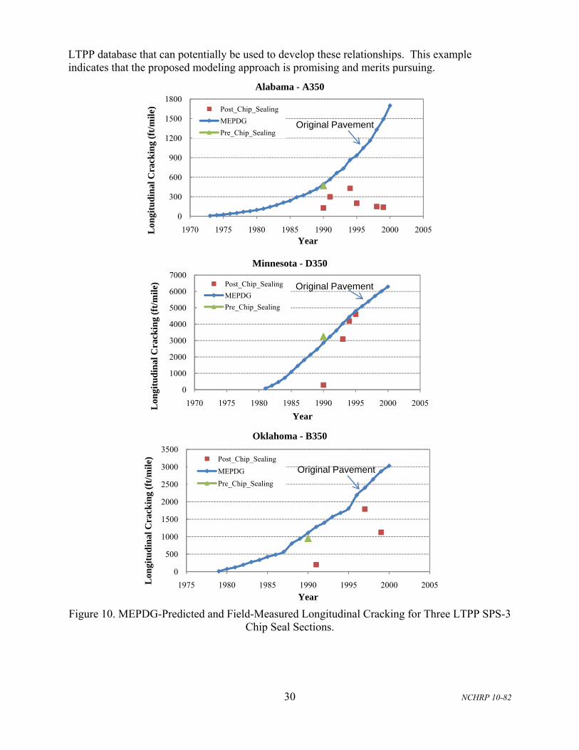
Example Performance Prediction Model for Diamond Grinding In these examples, the original PCC sections (located in Pennsylvania and Tennessee) were treated with diamond grinding in 1992 and 1996, respectively. Table 8 presents a summary of the original pavement design and site characteristics of these two sections.

32 NCHRP 10-82

Table 8. LTPP SPS-6 Diamond Grinding Sections Used for Testing Proposed Performance Prediction Modeling Approach.

Attributes Pennsylvania 42 0605 Tennessee 47 0605

Site Information:

Site Location I-80, Centre County I-40 Madison County Year of Original Construction 1968 1964

Functional Class1 (Rural Principal

Arterial–Interstate) 1 (Rural Principal

Arterial–Interstate) Latitude, Longitude 40.97, -77.79 35.72, -88.64

Initial Two-Way AADTT 4220 5560 Mean Annual Air Temp (ºF) 48.6 59.0

Freezing Index (ºF-days) 712.4 189.7 No. of Days below 32 ºF in a

Year133 75

Mean Annual Rainfall (in) 39.6 53.8 Average No. of Wet Days 180 154

Diamond Grinding Date 9/17/1992 6/7/1996

Layer Characteristics:

PCC Slab: Type JRCP JPCP

Thickness (in) 10.1 9.0 Dowel Diameter (in) 1.25 No Dowels

Contraction Spacing (ft) 61.5 25

Base:

Type Crushed Stone Soil Cement Thickness (in) 11 7.5

Subgrade:

Type Fine-Grained Soils: Silt Fine-Grained Soils: Lean

Inorganic Clay AASHTO Soil Class A-7-5 NA

CBR (%) 7 NA

The data shown in Table 8 were used as inputs to the MEPDG 1.1 software to predict faulting in the original PCC pavements. Similar to the chip seal examples, default values for some MEPDG inputs were used for variables that are not available in the LTPP database for these sections (e.g., traffic adjustment factors). Only joint faulting is used in this illustrative example. Figure 11 shows the MEPDG-predicted average joint faulting curve (for the original pavement) and the field-measured faulting values for the two PCC sections. In the Pennsylvania section, the green-triangle point represents the field-measured faulting immediately before diamond grinding was applied in 1992 (this data point was missing for the Tennessee section). The red-square points represent the field-measured average faulting in subsequent years after the diamond grinding was applied. The blue lines represent MEPDG-predicted average faulting in the original pavement (if the treatment was not applied). The next step is to develop mathematical relationships that link key diamond grinding quality characteristics (along with other variables that describe the original pavement and site conditions) to the magnitude of reduced distress throughout the treatment life. Table 9 shows diamond grinding quality characteristics available

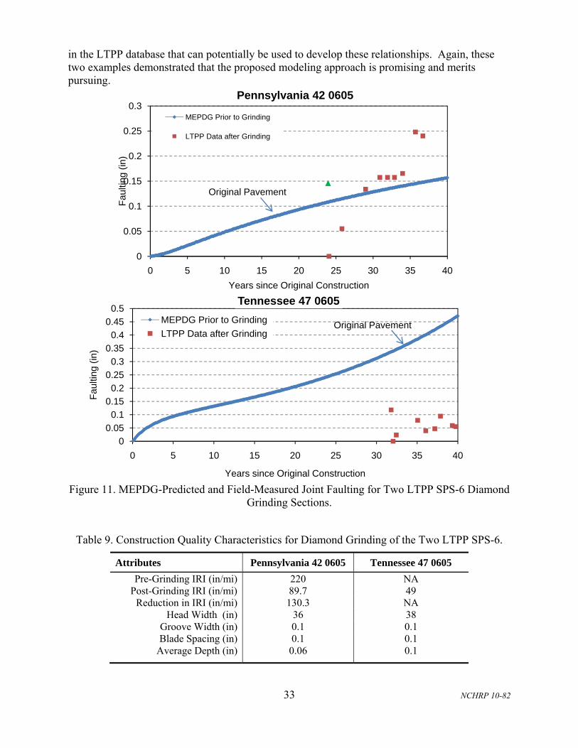
33 NCHRP 10-82

in the LTPP database that can potentially be used to develop these relationships. Again, these two examples demonstrated that the proposed modeling approach is promising and merits pursuing.

Figure 11. MEPDG-Predicted and Field-Measured Joint Faulting for Two LTPP SPS-6 Diamond

Grinding Sections.

Table 9. Construction Quality Characteristics for Diamond Grinding of the Two LTPP SPS-6.

Attributes Pennsylvania 42 0605 Tennessee 47 0605

Pre-Grinding IRI (in/mi) 220 NA Post-Grinding IRI (in/mi) 89.7 49

Reduction in IRI (in/mi) 130.3 NA Head Width (in) 36 38

Groove Width (in) 0.1 0.1 Blade Spacing (in) 0.1 0.1

Average Depth (in) 0.06 0.1

0

0.05

0.1

0.15

0.2

0.25

0.3

0 5 10 15 20 25 30 35 40

Fau

lting

(in

)

Years since Original Construction

Pennsylvania 42 0605

MEPDG Prior to Grinding

LTPP Data after Grinding

Original Pavement

0

0.05

0.1

0.15

0.2

0.25

0.3

0.35

0.4

0.45

0.5

0 5 10 15 20 25 30 35 40

Fau

lting

(in

)

Years since Original Construction

Tennessee 47 0605

MEPDG Prior to Grinding

LTPP Data after GrindingOriginal Pavement

34 NCHRP 10-82

Probabilistic Models

Since the available data can be noisy (i.e., highly variable with no clear patterns) and incomplete, it is best to use probabilistic modeling techniques for predicting in-service performance of treatments. Bayesian models are a promising technique in this situation. These models are generally developed by combining observed data and expert knowledge using Bayesian Networks (BNs). BNs are a formalism (founded in probability theory) for modeling problems involving uncertainty (Pearl 1988). A BN (which can often be understood in terms of cause-effect relationships) can be used for computing any probabilistic statement (conditional or not) of the involved variables. The influences and probabilistic interactions among variables that affect treatment performance can potentially be described in a BN. One feature that makes BNs particularly attractive in this case is that it is possible to start by defining a probability distribution from one source (e.g., expert knowledge), and then refining it later using another source (e.g., field data). The structure of a BN can be designed using knowledge of known causal dependences, influences, or correlations. All or part of these relationships may be derived from knowledge of domain experts, obtained from descriptions in the literature, or extracted from field data. Figure 12 shows a simple generic example BN. For example, the goal variable (X7) depends on the mediating variables (X5 and X6) and the mediating variable X5 is influenced by another mediating variable (X3). For each node (i.e., variable), there is a conditional probability function that relates this node to its parents. For instance, the probabilistic relationship between X4 and its parent X3 is the conditional probability distribution of X4 given X3 [i.e., P(X4|X3)].

Figure 12. Example Generic BN with Seven Variables.

Hajek and Bradbury (1996) described a Bayesian statistical analysis methodology for pavement deterioration modeling in the Canadian Strategic Highway Research Program (C-SHRP). In this application, several distress prediction models were constructed initially based on field data alone using linear regression techniques. After evaluation, the best one was selected for further analysis. Subsequently, five experts with 10 to 30 years of relevant experience and knowledge of past pavement surface failures containing steel slag aggregate were requested to rate the level of distress at different ages with different traffic and asphalt binder contents using a scale from 0 (no distress) to 10 (sufficient distress that unmistakably requires a rehabilitation treatment). Separate matrices for cracking and raveling were used since the distress index was considered as a linear function of cracking and raveling. The distress index (DI) matrices were then obtained

X1 X2

X3

X4X5

X6 X7

P(X1) P(X2)

P(X3|X1,X2)

P(X4|X3)P(X5|X3)

P(X7|X5,X6)P(X6|X4,X5)

35 NCHRP 10-82

by adding two matrices (each having 18 cells) coded by each expert. After carrying out a sensitivity analysis of these models, the final distress prediction model was selected. Hajeck and Bradbury (1996) stated that “the C-SHRP Bayesian statistical analysis software provides a unique feature that enables the user to obtain a probability density function for regression coefficients (for the data-based, expert-based, and combined models) and plot them in one composite figure for easy comparison.”

Data Availability and Quality

The LTPP database will be the primary source of data for developing performance prediction models for preservation treatments (a total of six treatments seemed most suitable for PRS). Ideally, the database should include treatment type, treatment year, treatment construction and materials quality characteristics, pre-treatment conditions, site conditions (traffic loading, climatic factors, subgrade type, etc.), and treatment performance (measured distresses and roughness). The research team has identified several promising sections for potential use in this research project. These sections were part of the LTPP experiments SPS-3, SPS-4, SPS-5, and SPS-6. The maps in Figures 13 and 14 show the number of these promising sections (grouped by state and treatment type) for HMA-surfaced and PCC-surfaced pavement, respectively.

Figure 13. Promising LTPP Sections of Preservation Treatments for HMA Pavement.

State having available LTPP chip seal data. In parenthesis is the number of LTPP sections.

WA (2)

MT (1)

ID (2)

CA (1)

NV (3)

UT (2)

AZ (4)

TX (13)

OK (3)

KS (1)

NE (1)

MN (4)

MI (1)

MO (1)

AR (1)TN (2)

MS(1)

AL (3)

FL (3)

Chip Seal

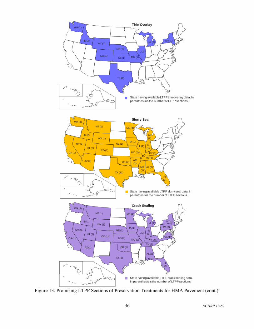
36 NCHRP 10-82

Figure 13. Promising LTPP Sections of Preservation Treatments for HMA Pavement (cont.).

State having available LTPPthin overlay data. In parenthesis is the number of LTPP sections.

TX (4)

NE (1)

CO (1)

ID (2)

IL (2)

KS (1)

MI (2)

MO (1)

NY (1)

WA (1)

WY (1)

Thin Overlay

AL (3)

TX (12)

AZ (4) AR (1)

CA (1)CO (1)

FL (3)

ID (2)

IL (1) IN (1)

IA (1)

KY (1)

MI (2)

MN (4)

MS (1)

MO (2)

MT (1)

NE (1)NV (3)

OK (3)

TN (3)

UT (2)

WA (3)

WY (1)

State having available LTPP slurry seal data. In parenthesis is the number of LTPP sections.

Slurry Seal

State having available LTPP crack sealing data. In parenthesis is the number of LTPP sections.

AL (2)

AZ (1)

CA (1)CO (1)

FL (2)

ID (1)

IL (2)IN (1)

IA (1)

KS (2)KY (2)

MI (1)

MN (4)

MO (2)

MT (1)

NE (1)NV (3)

NY (2)

OK (1)

PA (2)

TN (2)

TX (2)

UT (2)VA (1)

WA (3)

WY (1)

Crack Sealing

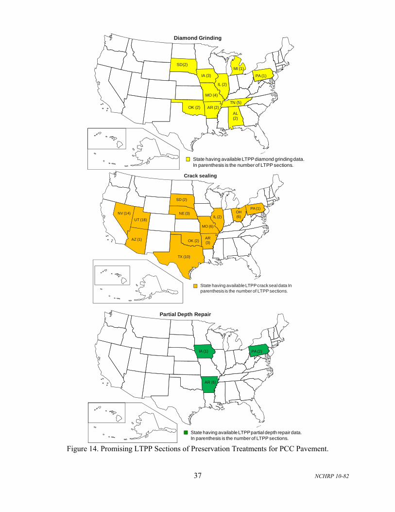
37 NCHRP 10-82

Figure 14. Promising LTPP Sections of Preservation Treatments for PCC Pavement.

State having available LTPP diamond grinding data. In parenthesis is the number of LTPP sections.

PA (1)

SD(2)

OK (2)

IA (3)

IL (2)

MI (1)

MO (4)

AR (2)TN (5)

AL (2)

Diamond Grinding

TX (10)

AZ (1) AR (3)

IL (2)OH (6)

PA (1)

MO (6)

NE (3)NV (14)

OK (2)

UT (18)

SD (2)

State having available LTPP crack seal data In parenthesis is the number of LTPP sections.

Crack sealing

State having available LTPP partial depth repair data. In parenthesis is the number of LTPP sections.

PA (2)IA (1)

AR (6)

Partial Depth Repair

38 NCHRP 10-82

Figure 14. Promising LTPP Sections of Preservation Treatments for PCC Pavement (cont.).

State having available LTPP full-depth repair data. In parenthesis is the number of LTPP sections.

PA (4)

SD(6)

OK (6)

IN(5)

MO (5)

AR (6)AZ (2)

Full-Depth Repair

State having available LTPP under seal repair data. In parenthesis is the number of LTPP sections.

OK (1)

TX (1)

CA (4)

Under Seal

State having available LTPP load transfer repair data. In parenthesis is the number of LTPP sections.

PA (4)

AL(2)

IN(5)

SD (2)

AR (2)AZ (1)

Load Transfer Restoration

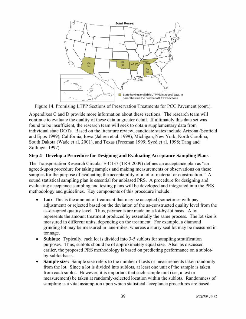
39 NCHRP 10-82

Figure 14. Promising LTPP Sections of Preservation Treatments for PCC Pavement (cont.).

Appendixes C and D provide more information about these sections. The research team will continue to evaluate the quality of these data in greater detail. If ultimately this data set was found to be insufficient, the research team will seek to obtain supplementary data from individual state DOTs. Based on the literature review, candidate states include Arizona (Scofield and Epps 1999), California, Iowa (Jahren et al. 1999), Michigan, New York, North Carolina, South Dakota (Wade et al. 2001), and Texas (Freeman 1999; Syed et al. 1998; Tang and Zollinger 1997).

Step 4 - Develop a Procedure for Designing and Evaluating Acceptance Sampling Plans

The Transportation Research Circular E-C137 (TRB 2009) defines an acceptance plan as “an agreed-upon procedure for taking samples and making measurements or observations on these samples for the purpose of evaluating the acceptability of a lot of material or construction.” A sound statistical sampling plan is essential for unbiased PRS. A procedure for designing and evaluating acceptance sampling and testing plans will be developed and integrated into the PRS methodology and guidelines. Key components of this procedure include:

Lot: This is the amount of treatment that may be accepted (sometimes with pay adjustment) or rejected based on the deviation of the as-constructed quality level from the as-designed quality level. Thus, payments are made on a lot-by-lot basis. A lot represents the amount treatment produced by essentially the same process. The lot size is measured in different units, depending on the treatment. For example, a diamond grinding lot may be measured in lane-miles; whereas a slurry seal lot may be measured in tonnage.

Sublots: Typically, each lot is divided into 3-5 sublots for sampling stratification purposes. Thus, sublots should be of approximately equal size. Also, as discussed earlier, the proposed PRS methodology is based on predicting performance on a sublot-by-sublot basis.

Sample size: Sample size refers to the number of tests or measurements taken randomly from the lot. Since a lot is divided into sublots, at least one unit of the sample is taken from each sublot. However, it is important that each sample unit (i.e., a test or measurement) be taken at randomly-selected location within the sublots. Randomness of sampling is a vital assumption upon which statistical acceptance procedures are based.

State having available LTPP joint reseal data. In parenthesis is the number of LTPP sections.

TN (3)

AL(2)

OK(3) AR (6)AZ

(1)

Joint Reseal

40 NCHRP 10-82

Acceptable Quality Level (AQL): This is the true quality level of a lot that the buyer (e.g., state DOT) is willing to accept at full payment to the contractor.

Rejectable Quality Level (RQL): This is the true quality level of a lot that the buyer (e.g., state DOT) considers so deficient that replacement or corrective action is warranted.

Maximum Allowable Quality Level (often referred to as M): A lot is rejected if the sample percent within limits (PWL) is less than M [or if the sample percent defective (PD) exceeds M]. Traditionally, M is set between RQL and AQL as an additional reliability to the constructed product and to provide balanced contractor and agency risks (AASHTO 2005 and AASHTO 1995).

Operating characteristic (OC) curves and expected pay curves will be used to evaluate acceptance sampling plans. These curves allow for determining the buyer’s and seller’s risks associated with the sampling plan (Weed 1994; Chamberlin 1995). The seller’s risk (α) is the risk of erroneously rejecting or assigning a payment decrease to a lot that indeed should be accepted or assigned a pay increase. The buyer’s risk (β) is the risk of erroneously accepting or not assigning a payment decrease to a lot that indeed should be rejected or assigned a pay decrease. The seller’s risk represents the contractor’s risk and the buyer’s risk represents the highway agency’s risk. Figure 15 shows a graphical representation of an OC curve.

Figure 15. Typical OC Curve.

The theoretical basis of statistical sampling plans is well-documented in the literature [see for example the Standard Recommended Practice for Acceptance Sampling Plans for Highway Construction (AASHTO Designations: R 9-90 and R 9-05), Buratti et al. 2004, and Duncan 1986]. The research team will build on this knowledgebase to develop specific guidelines for developing acceptance plans for pavement preservation PRS.

Step 5 – Evaluate and Refine the PRS Methodology and Guidelines

Since the final guidelines will be developed based on the PRS methodology discussed earlier, it is important to evaluate this methodology as a whole system (not as separate components). The research team will integrate the PRS methodology into a simulation-based software tool, so that it can be tested, verified, and refined (as needed). This software tool will be developed as a research tool (not as a commercial software application). A comprehensive sensitivity analysis will be designed and performed on the methodology to uncover errors, understand its limitations, and improve it.

0

100

0 100

Pro

bab

ilit

y of

Acc

epta

nce

, %

Percent within Limits (PWL), %

Agency Risk,

Contractor's Risk,

AQLRQL

41 NCHRP 10-82

Finally, the PRS methodology and guidelines will be demonstrated through illustrative examples. These examples will be designed to illustrate the use of the PRS guidelines for different preservation treatments (six treatment found most suitable for PRS), pavement types (HMA-surfaced pavement and PCC-surfaced pavement), highway classification (high, medium, and low traffic volumes), and climatic regions.

42 NCHRP 10-82

CHAPTER 5 A PROCESS FOR ASSESSING THE SUITABILITY OF PAVEMENT PRESERVATION TREATMENTS FOR PRS

This chapter presents a process for assessing the suitability of pavement preservation treatments for PRS using the Analytic Hierarchy Process.

ANALYTIC HIERARCHY PROCESS Several multi-criteria decision analysis and ranking methods have been identified for possible use in ranking preservation treatments based on their suitability for PRS. These methods include the Analytic Hierarchy Process, Direct Weighting Method, Observer-Derived Weights Method, Multi-Attribute Utility Theory, Swing Weighting Method, and Indifference Trade-off Weighting Method. The details of these methods are available in the literature (see for example, Sinha et al. 2009; Huber 1974; Hobbs 1980; Keeney and Raiffa 1993). Based the pros and cons of these methods, as identified in the literature, AHP has been selected for assessing the suitability of pavement preservation treatments for PRS. AHP has been selected for the following primary reasons:

Its ability to handle multi-criteria decision-making problems. Its ability to consider both qualitative and quantitative input parameters. Its computational process is robust, and at the same time, is relatively simple to perform.

AHP was originally developed in the early 1970s to deal with unstructured decision-making problems in contingency planning at the Department of Defense (Saaty 1980; Saaty 1990b). AHP requires formulating the decision problem in a hierarchal fashion. The hierarchy consists of the decision objective at the highest level, a set of alternatives, at the bottom or last level, and a set of evaluation criteria at mid-level that relate the alternatives to the objective. The evaluation criteria can be broken down into multiple sub-criteria, depending on the complexity of the decision problem. The elements at each level are placed in a pairwise matrix, where each element is compared against each other element. The pairwise comparisons are made using a predefined importance rating scale (Saaty 1990b). This importance rating scale ranges from 1 to 9. The odd numbers (1, 3, 5, 7, and 9) represent the primary importance intensity values, while the even numbers, 2, 4, 6, and 8 represent intermediate importance intensity values. Table 10 illustrates this rating scale. The elements are not compared to the decision as a whole; rather they are compared with each other to determine how they compete for importance in making the final decision. The pairwise comparison builds an n×n judgment matrix (called A matrix); where n is the number of elements being compared.

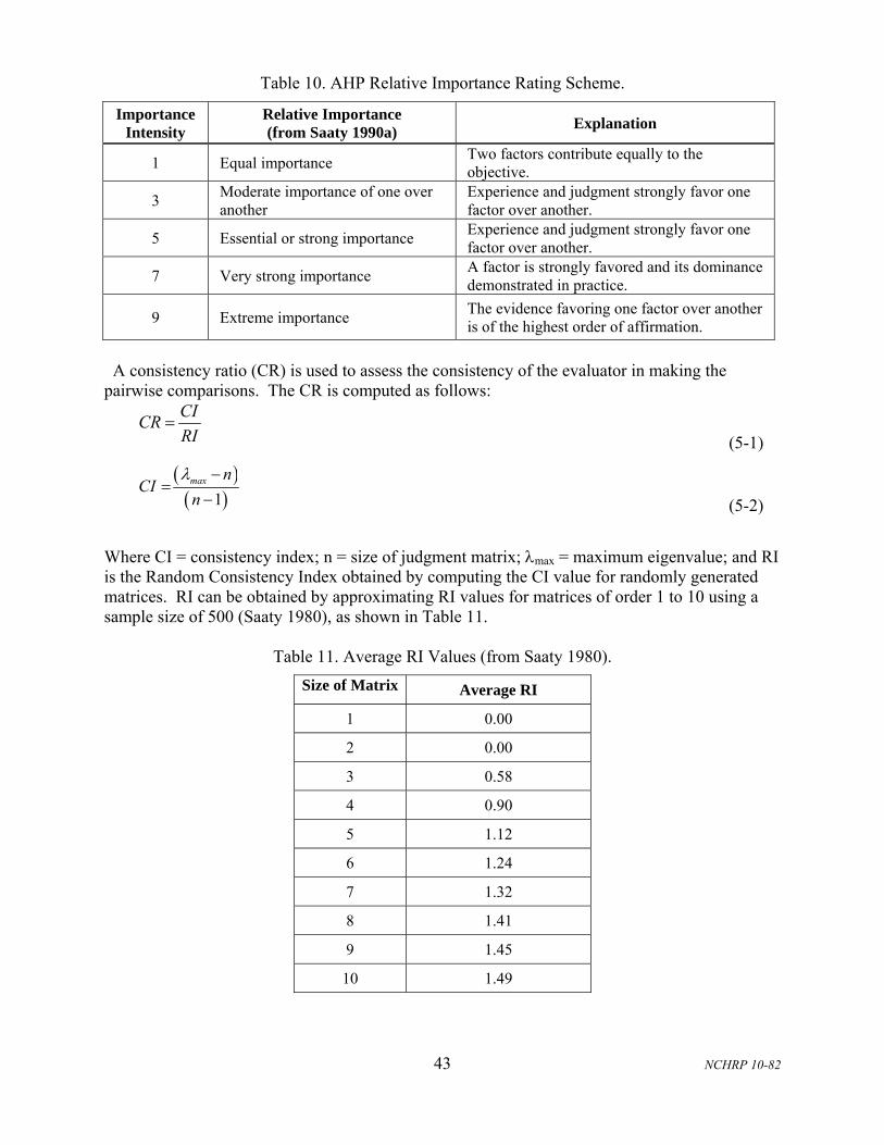
43 NCHRP 10-82

Table 10. AHP Relative Importance Rating Scheme.

Importance Intensity

Relative Importance (from Saaty 1990a)

Explanation

1 Equal importance Two factors contribute equally to the objective.

3 Moderate importance of one over another

Experience and judgment strongly favor one factor over another.

5 Essential or strong importance Experience and judgment strongly favor one factor over another.

7 Very strong importance A factor is strongly favored and its dominance demonstrated in practice.

9 Extreme importance The evidence favoring one factor over another is of the highest order of affirmation.

A consistency ratio (CR) is used to assess the consistency of the evaluator in making the pairwise comparisons. The CR is computed as follows:

CICR

RI

(5-1)

1max n

CIn

(5-2)

Where CI = consistency index; n = size of judgment matrix; max = maximum eigenvalue; and RI is the Random Consistency Index obtained by computing the CI value for randomly generated matrices. RI can be obtained by approximating RI values for matrices of order 1 to 10 using a sample size of 500 (Saaty 1980), as shown in Table 11.

Table 11. Average RI Values (from Saaty 1980).

Size of Matrix Average RI

1 0.00

2 0.00

3 0.58

4 0.90

5 1.12

6 1.24

7 1.32

8 1.41

9 1.45

10 1.49

44 NCHRP 10-82

Saaty (1990b) suggests that the CR should be less than 10%. This CR threshold value essentially implies that the method allows for up to 10% error in human judgment during the pairwise comparison phase. Once the judgment matrix passes the consistency check, the weights associated with the elements being compared are computed in a process known as “synthesis.” This process involves computing the principal eigenvector associated with the maximum eigenvalue for the pairwise matrix A. This principal eigenvector is normalized to create a relative ratio scale that can be used as the priority weight vector (called w) or more simply put, weights associated with each element being compared. The calculation of an eigenvalue and eigenvector are not discussed here for brevity; but they can be found in most algebra textbook. A priority weight vector w is established for each criterion, sub-criterion, as well as the alternatives under each sub-criterion.

AHP STRUCTURE Figures 16 and 17 show the decision hierarchy for assessing the suitability of pavement preservation treatments for PRS for HMA-surfaced and PCC-surfaced pavements, respectively. Each hierarchy consists of the following layers:

Objective (Level 1): The objective is “to select the three most suitable treatments for inclusion in the PRS guide for pavement preservation.”

Evaluation Criteria (Level 2): The evaluation criteria consist of five factors, as follows: o Availability of initial AQCs. o Availability of data that can be used for correlating initial AQCs with in-service

performance. o Reliability of performance prediction models that link initial AQCs to in-service

performance. o Ability to consider the effect of existing pavement condition on treatment

performance. o Industry and DOT willingness to accept and implement PRS.

Treatment (Level 3): For HMA-surfaced pavements, eight treatments are included at this level of the hierarchy. For PCC-surfaced pavements, seven treatments are included.

The decision-making task is to determine the three most suitable treatments for PRS, considering the above evaluation criteria. A judgment matrix for the evaluation level (Level 2) will be established to determine a priority weight for each evaluation criterion. Also, judgment matrixes will be established for the preservation treatments based on each evaluation criterion (i.e., five judgment matrixes for HMA-surfaced pavement and five judgment matrixes for PCC-surfaced pavements). Finally, a priority score will be computed for each treatment based on the pairwise comparisons of all judgment matrixes. Treatments with the highest three priority scores (for each pavement type) will be deemed as most suitable for PRS. This process is best demonstrated through an example, as discussed in the following section of this chapter.

45 NCHRP 10-82

Figure 16. AHP for Assessing the Suitability of HMA Pavement Preservation Treatments for PRS.

Figure 17. AHP for Assessing the Suitability of PCC Pavement Preservation Treatments for PRS.

DEMONSTRATION EXAMPLE

(This example is hypothetical and is intended for demonstration purposes only.) Figure 18 shows Level 2 judgment matrix for the demonstration example. In this hypothetical example, the result of comparing “suitability of initial AQCs for PRS” to “availability of data on

SS=Slurry Seals; CS=Chip Seals; FS=Fog Seals; CrS=Crack sealing; Ms=Microsurfacing; TOL=Thin HMAOverlay; CR=Cold in‐place recycling; HR=Hot in‐place recycling

Availability of initial AQCsappropriate

for PRS

Availability of data on initial AQCs & in‐service performance

Reliability of performance

prediction models

Ability to consider the effect of existing pavement condition on

treatment performance

Treatment Use

Select the three most suitable treatments for inclusion in the PRS

guidelines for pavement preservation

MsCS TOLFS CrS CRSS HR

Availability of initial AQCsappropriate

for PRS

Availability of data on initial AQCs & in‐service performance

Reliability of performance

prediction models

Ability to consider the effect of existing pavement condition on


Treatment Use

Select the three most suitable treatments for inclusion in the PRS

guidelines for pavement preservation

DGPDR TOLUS LTR JR CrS

PDR=Partial‐Depth Repair; US=Undersealing (or Slab Stabilization); LTR=Load Transfer Restoration; DG=Diamond GrindingTOL=Thin HMAOverlay; JR=Joint Resealing; CrS= Crack Sealing

46 NCHRP 10-82

initial AQCs & in-service performance” is 2, which indicates that the importance of “suitability of initial AQCs for PRS” to the evaluator is two times that of the “availability of data on initial AQCs & in-service performance.” On the other hand, the result of comparing “availability of data on initial AQCs & in-service performance” to “treatment use” is 1/2, which indicates that the importance of “availability of data on initial AQCs & in-service performance” is half that of the “treatment use.”

Figure 18. Level 2 Judgment Matrixes for the Demonstration Example.

The CR of this example judgment matrix is 6.8% (computed using Equations 5-1 and 5-2), which is less than the 10% threshold value. Thus, the matrix passes the consistency check and the priority weights can be computed. The final weights for the evaluation elements are calculated using the synthesis procedure mentioned earlier and are shown in Table 12.

Table 12. Weights for Each Evaluation Criterion in the Demonstration Example.

Evaluation Criterion No.

Evaluation Criterion Priority Weight

1 Suitability of initial AQCs for PRS 0.35

2 Availability of data on initial AQCs & in-service performance 0.21

3 Availability and reliability of performance prediction models 0.05

4 Ability to consider the effect of existing pavement condition on treatment performance

0.07

5 Treatment Use 0.32

Figure 19 shows five hypothetical judgment matrixes for the PCC-surfaced pavement preservation treatments (Level 3 in the AHP hierarchy). The CR values for these hypothetical matrixes range between 4% and 7.1%, which are less than the 10% threshold value. Thus, these matrixes pass the consistency check and a weight can be computed for each treatment based on each evaluation criterion. Table 13 shows these weights.

Evaluation Criteria

Suitability of

initial AQCs for

PRS

Availability of

data on initial

AQCs & in‐service

performance

Availability and

reliability of

performance

prediction models

Ability to consider the

effect of existing

pavement condition

on treatment

performance

Treatment Use

Suitability of initial AQCs

for PRS1 2 4 3 2

Availability of data on

initial AQCs & in‐service

performance1 5 4 1/2

Availability and reliability

of performance prediction

models1 1/2 1/5

Ability to consider the

effect of existing

pavement condition on


1 1/7

Treatment Use 1

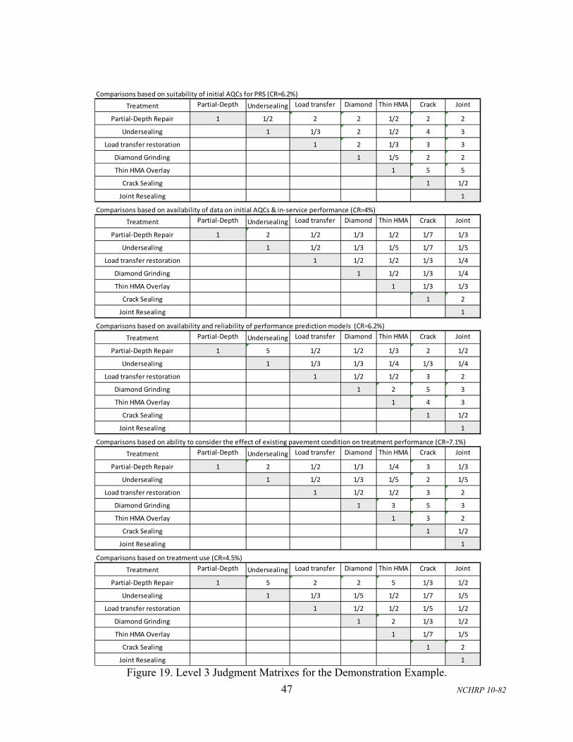
47 NCHRP 10-82

Figure 19. Level 3 Judgment Matrixes for the Demonstration Example.

Comparisons based on suitability of initial AQCs for PRS (CR=6.2%)

Treatment Partial‐Depth Undersealing Load transfer Diamond Thin HMA Crack Joint

Partial‐Depth Repair 1 1/2 2 2 1/2 2 2

Undersealing 1 1/3 2 1/2 4 3

Load transfer restoration 1 2 1/3 3 3

Diamond Grinding 1 1/5 2 2

Thin HMA Overlay 1 5 5

Crack Sealing 1 1/2

Joint Resealing 1

Comparisons based on availability of data on initial AQCs & in‐service performance (CR=4%)


Partial‐Depth Repair 1 2 1/2 1/3 1/2 1/7 1/3

Undersealing 1 1/2 1/3 1/5 1/7 1/5

Load transfer restoration 1 1/2 1/2 1/3 1/4

Diamond Grinding 1 1/2 1/3 1/4

Thin HMA Overlay 1 1/3 1/3

Crack Sealing 1 2

Joint Resealing 1

Comparisons based on availability and reliability of performance prediction models (CR=6.2%)


Partial‐Depth Repair 1 5 1/2 1/2 1/3 2 1/2

Undersealing 1 1/3 1/3 1/4 1/3 1/4

Load transfer restoration 1 1/2 1/2 3 2

Diamond Grinding 1 2 5 3


Crack Sealing 1 1/2

Joint Resealing 1

Comparisons based on ability to consider the effect of existing pavement condition on treatment performance (CR=7.1%)


Partial‐Depth Repair 1 2 1/2 1/3 1/4 3 1/3

Undersealing 1 1/2 1/3 1/5 2 1/5

Load transfer restoration 1 1/2 1/2 3 2

Diamond Grinding 1 3 5 3


Crack Sealing 1 1/2

Joint Resealing 1

Comparisons based on treatment use (CR=4.5%)


Partial‐Depth Repair 1 5 2 2 5 1/3 1/2

Undersealing 1 1/3 1/5 1/2 1/7 1/5

Load transfer restoration 1 1/2 1/2 1/5 1/2

Diamond Grinding 1 2 1/3 1/2

Thin HMA Overlay 1 1/7 1/5

Crack Sealing 1 2

Joint Resealing 1

48 NCHRP 10-82

Table 13. Weights for Each Treatment Based on Each Evaluation Criterion in the Demonstration

Example.

Treatment Evaluation Criterion No.

1 2 3 4 5

Partial-Depth Repair 0.15 0.05 0.11 0.08 0.16

Undersealing 0.16 0.04 0.04 0.06 0.03

Load transfer restoration 0.18 0.08 0.16 0.15 0.07

Diamond Grinding 0.08 0.11 0.28 0.31 0.11

Thin HMA Overlay 0.32 0.13 0.24 0.22 0.06

Crack Sealing 0.05 0.33 0.06 0.05 0.35

Joint Researing 0.06 0.26 0.12 0.14 0.21

The final step in the process is to apply the weights for each evaluation criterion to each of the treatment priority vectors and sum across to determine a priority score for each treatment. Table 14 shows the treatment priority scores. For this hypothetical demonstration example, Thin HMA Overlay, Crack Sealing, and Joint Resealing have the highest three priority scores.

Table 14. Treatments Priority Scores for the Demonstration Example.

Treatment Priority Score (0-1.0)

Partial-Depth Repair 0.13

Undersealing 0.08

Load transfer restoration 0.12

Diamond Grinding 0.12

Thin HMA Overlay 0.19

Crack Sealing 0.21

Joint Researing 0.16

AHP EVALUATORS The pairwise comparisons can be made through direct interviews or survey questionnaires of evaluators who are familiar with the decision problem. However, to obtain reliable comparisons; the evaluators must have sufficient information on the factors they are asked to consider. For example, the evaluators must have a good understanding of what makes an AQC suitable for PRS to be able to compare the importance of “suitability of initial AQCs for PRS” to each other element in the judgment matrix. Also, the evaluators must have a good understanding of existing data on each treatment to be able to compare treatments based on “availability of data.” Therefore, it is proposed that these comparisons be made by the research team and possibly members of the project panel.

49 NCHRP 10-82

CHAPTER 6 CLOSURE

This interim report provides a summary of the work that has been completed to date and a plan for future work to be completed under NCHRP project 10-82 (Performance-Related Specifications for Pavement Preservation Treatments). The objective of this research is to develop guidelines for use in preparing performance-related specifications for pavement preservation treatments. Chapter 1 discusses the background of the research problem, and describes the research objectives and the need for the PRS guidelines. It also presents the scope of work for this research project, in terms of the phases and tasks. Chapter 2 summarizes key findings of a very extensive literature review undertaken in Task 1 of the project. Numerous publications related to pavement preservation (design, construction, materials, and performance), PRS for pavements, and pavement performance prediction modeling were gathered and reviewed in this task. Chapter 3 discusses current specifications for pavement preservation treatments, with emphasis on acceptance quality characteristics that are measured during or immediately after construction. This work was undertaken in Task 1 of the project. Chapter 4 presents a detailed outline of the PRS guidelines and a step-by-step plan for developing them. The plan describes a detailed PRS methodology, including a promising approach for modeling the performance of preservation treatments. Additionally, examples are presented and potential data sources for developing these models are identified in this chapter. Chapter 5 provides a systematic process for assessing the suitability of pavement preservation treatments for PRS based on the Analytic Hierarchy Process. A total of six preservation treatments deemed most suitable for PRS will be identified using this process. The guidelines will be developed for these six treatments. The report includes four appendixes. Appendix A includes summary tables of current specifications for preservation treatments for HMA-surfaced and PCC-surfaced pavements. Appendix B provides a bibliography of existing performance prediction models for both HMA and PCC pavements. Appendixes C and D contain site condition data for promising HMA and PCC treatment sections obtained from the Long-Term Pavement Performance database.

50 NCHRP 10-82

REFERENCES

American Association of State Highway and Transportation Officials (AASHTO). (2005). Standard Recommended Practice for Acceptance Sampling Plans for Highway Construction, AASHTO Designation R9-05, Washington, D.C.

American Association of State Highway and Transportation Officials (AASHTO). (1995). Standard Recommended Practice for Acceptance Sampling Plans for Highway Construction. AASHTO Designation R9-90, Washington, D.C.

American Concrete Pavement Association (ACPA). (1993). Joint and Crack Sealing and Repair for Concrete Pavements. Technical Bulletin TB-012P. American Concrete Pavement Association, Skokie, IL.

American Concrete Pavement Association (ACPA). (1994). Slab Stabilization Guidelines for Concrete Pavements. Technical Bulletin TB-018P. American Concrete Pavement Association, Skokie, IL.

Anderson, D.A., Luhr, D.R., and Antle, C.E. (1990). Framework for Development of Performance-Related Specifications for Hot-Mix Asphaltic Concrete, NCHRP Report 332, Transportation Research Board, National Research Council, Washington, D.C.

Applied Research Associates (ARA). (2004). Guide for Mechanistic-Empirical Design of New and Rehabilitated Pavement Structures (Final Report), National Cooperative Highway Research Program, http://www.trb.org/mepdg/guide.htm, accessed: December 1, 2010.

Burati, J.L., Weed, R. M., Hughes, C. S., and Hill, H. S. (2004). “Optimal Procedures for Quality Assurance Specifications,” Federal Highway Administration, Publication No. FHWA-RD-02-095, McLean, VA.

Buch, N., Barnhart, V., and Kowli, R. (2003). “Precast Concrete Slabs as Full-Depth Repairs: Michigan Experience.” Journal Transportation Research Record: Journal of the Transportation Research Board, Vol. 1823, Transportation Research Board of the National Academies, Washington, D.C., pp. 55–63.

Bullard, D.J., Smith, R.E., and Freeman, T.J. (1992). Development of a Procedure to Rate the Application of Pavement Maintenance Treatments. Report No. SHRP-M/FR-92-102, Strategic Highway Research Program (SHRP), National Research Council, Washington D.C.

Chamberlin, W. P. (1995). Performance-Related Specifications for Highway Construction and Rehabilitation. NCHRP Synthesis of Highway Practice 212, Transportation Research Board, Washington, D.C.

Cuelho, E., Mokwa, R., and Akin, M. (2006). Preventive Maintenance Treatments of Flexible Pavements: A Synthesis of Highway Practice. Report No. FHWA/MT-06-009/8117-26, Montana Department of Transportation, Montana.

Duncan, A. J. (1986). “Quality Control and Industrial Statistics,” R.D. Irwin, ISBN 0256035350, Fifth Edition, 1986.

El-Basyouny, M., and Jeong, M.G. (2010). “Probabilistic Performance-Related Specifications Methodology Based on Mechanistic–Empirical Pavement Design Guide.” Transportation Research Record: Journal of the Transportation Research Board, No. 2151, Transportation Research Board of the National Academies, Washington, D.C., pp. 93–102.

51 NCHRP 10-82

Epps, J.A, Hand, A., Seeds, S., Scholz, T., Ashmore, C., Monismith, C.L., Deacon, J.A., Harvey, J.T., and Leahy, R. (2002). “Recommended Performance-Related Specifications for Hot-Mix Asphalt Construction: Results of the WesTrack Project,” NCHRP 455, National Cooperative Highway Research Program, Washington, D.C.

Federal Highway Administration (FHWA) (1999). Pavement Preservation: A Road Map for the Future, Publication No. FHWA-SA-99-015, Federal Highway Administration, Washington, D.C.

Federal Highway Administration (FHWA) (2005). Pavement Preservation Definitions, Memorandum, http://www.fhwa.dot.gov/pavement/preservation/091205.cfm. Accessed February 7, 2011.

Freeman, T. J. (1999). “Supplemental Maintenance Effectiveness Research Program (SMERP).” Presentation at the AGC Pavement Preservation Seminar, October 4–5, Austin, TX.

Galehouse, L. (2002). “Strategic Planning for Pavement Preventive Maintenance: Michigan Department of Transportation’s ‘Mix of Fixes’ Program,” TR News, March–April 2002, Number 219, Transportation Research Board, National Research Council, Washington, D.C.

Gransberg, D.D. (2010). Microsurfacing: A Synthesis of Highway Practice, NCHRP Synthesis 411, National Cooperative Highway Research Program, Transportation Research Board, Washington, DC.

Hajek, J.J, and Bradbury, A. (1996). “Pavement Performance Modeling using Canadian Strategic Highway Research Program Bayesian Statistical Methodology,” Transportation Research Record: Journal of the Transportation Research Board, No. 1524, Transportation Research Record No. 1524, pp.160.

Hobbs, B. F. (1980). “A Comparison of Weighting Methods in Power Plant Siting.” Decision Sci., 11, 725–737.

Hoerner, T.E., and Darter, M.I. (1999). Guide to Developing Performance-Related Specifications for PCC Pavements, Volume I. FHWA Report FHWA-RD-98-155, Federal Highway Administration: McLean, Virginia.

Hoerner, T.E., Darter, M.I., Khazanovich, L., Titus-Glover T., and Smith, K.L. (2000). Improved Prediction Models for PCC Pavement Performance-Related Specifications, Volume I, FHWA Report FHWA-RD-00-130, Federal Highway Administration: McLean, Virginia.

Huang, Y.H. (2004). Pavement Analysis and Design, Second Edition, Pearson Prentice Hall: Upper Saddle River, N.J.

Huber, G.P. (1974). “Methods for Quantifying Subjective Probabilities and Multi-attribute Utilities.” Decision Sci., 53, 430–458.

Jahren, C. K., Bergeson, K., Al-Hammadi, A, Celik, S., and Lau, G. (1999). “Thin Maintenance Surfaces.” Phase One Report, Center for Transportation Research and Education, Iowa State.

Jeong, M.G. and El-Basyouny, M. (2010). “Statistical Applications and Stochastic Analysis for Performance-Related Specification of Asphalt Quality Assurance,” Transportation Research Record: Journal of the Transportation Research Board, No. 2151, Transportation Research Board of the National Academies, Washington, D.C., pp. 84–92.

Keeney, R. L., and Raiffa, H. (1993). Decision with Multiple Objectives: Preferences and Value Tradeoffs, Wiley, New York.

52 NCHRP 10-82

Morian, D.A. (2011). Cost Benefit Analysis of Including Microsurfacing in Pavement Treatment Strategies & Cycle Maintenance, Final Report No. FHWA-PA-2011-001-080503, Pennsylvania Department of Transportation, Pennsylvania.

Pearl, J. (1988). Probabilistic Reasoning in Intelligent Systems. Morgan Kaufman, San Mateo, California.

Peshkin, D.G., Hoerner, T.E., and Zimmerman, K.A. (2004). Optimal Timing of Pavement Preventive Maintenance Treatment Applications, NCHRP Report 523, National Cooperative Highway Research Program, Transportation Research Board, Washington, D.C.

Saaty, T. L. (1980). The Analytic Hierarchy Process, McGraw-Hill, New York, NY.

Saaty, T. L. (1990a). “How to Make a Decision: the Analytic Hierarchy Process.” Eur.J.Oper.Res., 48(1), 9–26.

Saaty, T. L. (1990b). “Multicriteria Decision Making: the Analytic Hierarchy Process: Planning, Priority Setting, Resource Allocation.” RWS publications, Pittsburgh, PA.

Scofield, L. and Epps, J. (1999). “Survey of Pavement Maintenance Practices in Arizona.” Draft Report, Arizona Department of Transportation, Phoenix, AZ.

Seeds, S.B., Basavaraju, R., Epps, J.A., and Weed, R.M. (1997). Development of Performance-Related Specifications for Hot-Mix Asphalt Pavements Through WesTrack, Transportation Research Record: Journal of the Transportation Research Board, No. 1575, Transportation Research Board of the National Academies, Washington, D.C., pp. 85-91.

Sinha K.C., Patidar V., Li Z., and S. Labi, (2009). “Establishing the Weights of Performance Criteria: Case Studies in Transportation Facility Management.” Journal of Transportation Engineering, Vol. 135, No. 9, September 2009, pp. 619–631.

Smith, R. E. (2002). “Integrating Pavement Preservation into a Local Agency Pavement Management System.” Transportation Research Record: Journal of the Transportation Research Board, No. 1795, Transportation Research Board of the National Academies, Washington, D.C., pp. 27–32.

Smith, R.E., Freeman, T.J., and Pendleton, O. (1993). Pavement Maintenance Effectiveness. Report No. SHRP-H-358, Strategic Highway Research Program (SHRP), National Research Council, Washington D.C.

Smith, K.L. and Peshkin, D.G. (2011). “Pavement Preservation on High Traffic Volume Roadways,” Proceedings of the Transportation Research Board 90th Annual Meeting, Washington, D.C., January 23-27, 2011.

Syed, I. M., Freeman, T. J., and Smith, R. E. (1998). “Effectiveness of Highway Maintenance Treatments Used in Texas.” Flexible Pavement Rehabilitation and Maintenance, Special Technical Publication (STP) 1348, American Society for Testing and Materials, West Conshohocken, PA.

Tang, T. and D.G. Zollinger. (1997). Investigation of Spall Repair for Concrete Pavements. Research Report TX-98/2919-3, TTI 2919-3, Texas Transportation Institute, The Texas A&M University System, Texas Department of Transportation.

Transportation Research Board (TRB) (2009). “Glossary of Highway Quality Assurance Terms,” Transportation Research Board, Electronic Circular E-C137, 4th Update, Washington, D.C.

53 NCHRP 10-82

Wade, M., DeSombre, R., and Peshkin, D. (2001). “High Volume/High Speed Asphalt Roadway Preventive Maintenance Treatments.” Publication No. SD99-09, South Dakota Department of Transportation, Pierre, SD.

Weed, R.M. (1989). Statistical Specification Development, Report No. FHWA/NJ-88-017, New Jersey Department of Transportation, Trenton, N.J., 1989.

Weed, R.M. (1994). “Adjusted Pay Schedules: New Concepts and Provisions,” Transportation Research Record: Journal of the Transportation Research Board, No. 1465, Transportation Research Board of the National Academies, Washington, D.C., pp. 9–15.

Weed, R.M. (2006). “Mathematical Modeling Procedures for Performance-Related Specifications,” Transportation Research Record: Journal of the Transportation Research Board, No. 1946, Transportation Research Board of the National Academies, Washington, D.C., pp. 63–70.

Zhang, Z., Jaipuria, S., Murphy, M.R., Sims, T. and Garza, T. Jr. (2010). “Pavement Preservation: Performance Goal and Its Implications.” Transportation Research Record: Journal of the Transportation Research Board, No. 2150, Transportation Research Board of the National Academies, Washington, D.C., pp. 28–35.

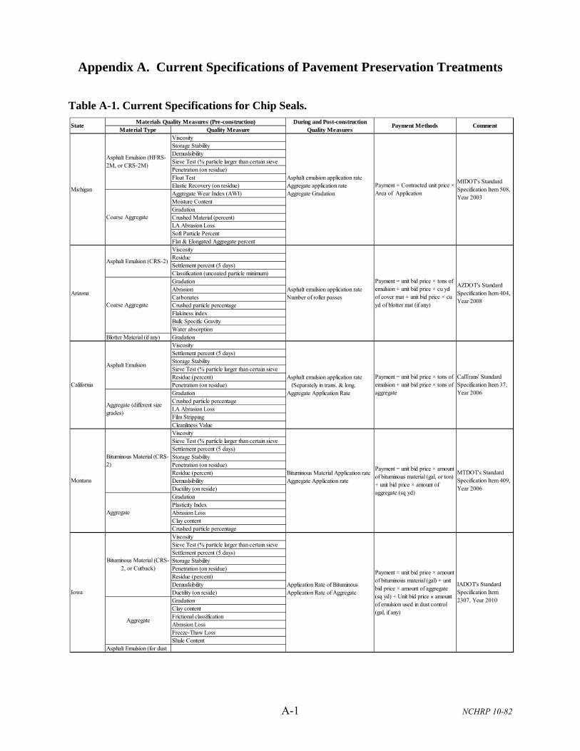
A-1 NCHRP 10-82

Appendix A. Current Specifications of Pavement Preservation Treatments

Table A-1. Current Specifications for Chip Seals.

Material Type Quality MeasureViscosityStorage StabilityDemuslsibilitySieve Test (% particle larger than certain sieve Penetration (on residue)Float Test Asphalt emulsion application rateElastic Recovery (on residue) Aggregate application rateAggregate Wear Index (AWI) Aggregate GradationMoisture ContentGradationCrushed Material (percent)LA Abrasion LossSoft Particle PercentFlat & Elongated Aggregate percentViscosityResidue Settlement percent (5 days)Classification (uncoated particle minimum)GradationAbrasion Asphalt emulsion application rateCarbonates Number of roller passesCrushed particle percentageFlakiness indexBulk Specific GravityWater absorption

Blotter Material (if any) GradationViscositySettlement percent (5 days)Storage StabilitySieve Test (% particle larger than certain sieve Residue (percent) Asphalt emulsion application ratePenetration (on residue) (Separately in trans. & long. Gradation Aggregate Application RateCrushed particle percentageLA Abrasion LossFilm StrippingCleanliness ValueViscositySieve Test (% particle larger than certain sieve Settlement percent (5 days)Storage StabilityPenetration (on residue)Residue (percent) Bituminous Material Application rateDemuslsibility Aggregate Application rateDuctility (on reside)GradationPlasticity IndexAbrasion LossClay contentCrushed particle percentageViscositySieve Test (% particle larger than certain sieve Settlement percent (5 days)Storage StabilityPenetration (on residue)Residue (percent)Demuslsibility Application Rate of Bituminous Ductility (on reside) Application Rate of AggregateGradationClay contentFrictional classificationAbrasion LossFreeze-Thaw LossShale Content

Asphalt Emulsion (for dust

Payment Methods CommentStateMaterials Quality Measures (Pre-construction) During and Post-construction

Quality Measures

Iowa

California

MTDOT's Standard Specification Item 409, Year 2006

Payment = unit bid price × amount of bituminous material (gal, or ton) + unit bid price × amount of aggregate (sq yd)

IADOT's Standard Specification Item 2307, Year 2010

Michigan

Arizona

Asphalt Emulsion (CRS-2)

Montana

Asphalt Emulsion

Aggregate (different size grades)

MIDOT's Standard Specification Item 508, Year 2003

Payment = Contracted unit price × Area of Application

Coarse Aggregate

Asphalt Emulsion (HFRS-2M, or CRS-2M)

Aggregate

Bituminous Material (CRS-2)

CalTrans' Standard Specification Item 37, Year 2006

Payment = unit bid price × tons of emulsion + unit bid price × tons of aggregate

AZDOT's Standard Specification Item 404, Year 2008

Coarse Aggregate

Payment = unit bid price × amount of bituminous material (gal) + unit bid price × amount of aggregate (sq yd) + Unit bid price × amount of emulsion used in dust control (gal, if any)

Payment = unit bid price × tons of emulsion + unit bid price × cu yd of cover mat + unit bid price × cu yd of blotter mat (if any)

Bituminous Material (CRS-2, or Cutback)

Aggregate

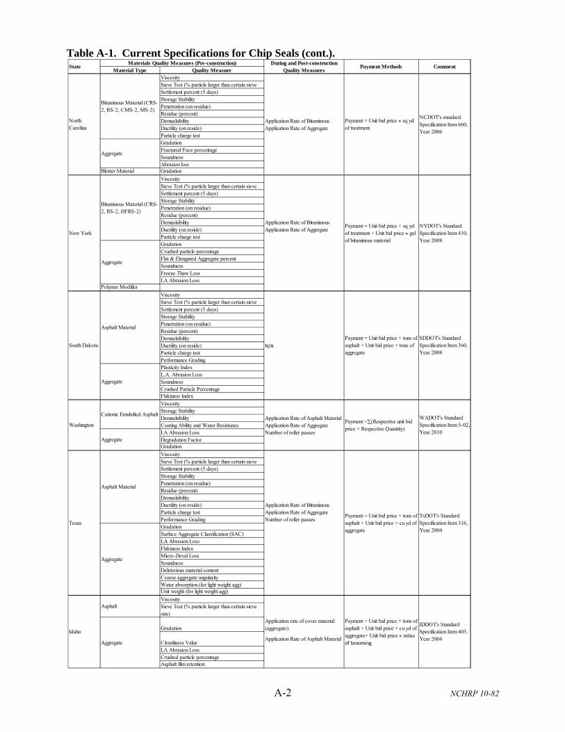
A-2 NCHRP 10-82

Table A-1. Current Specifications for Chip Seals (cont.).

Material Type Quality MeasureViscositySieve Test (% particle larger than certain sieve Settlement percent (5 days)Storage StabilityPenetration (on residue)Residue (percent)Demuslsibility Application Rate of Bituminous Ductility (on reside) Application Rate of AggregateParticle charge testGradationFractured Face percentageSoundnessAbrasion loss

Blotter Material Gradation

ViscositySieve Test (% particle larger than certain sieve Settlement percent (5 days)Storage StabilityPenetration (on residue)Residue (percent)Demuslsibility Application Rate of Bituminous Ductility (on reside) Application Rate of AggregateParticle charge testGradationCrushed particle percentageFlat & Elongated Aggregate percentSoundnessFreeze-Thaw LossLA Abrasion Loss

Polymer Modifier

ViscositySieve Test (% particle larger than certain sieve Settlement percent (5 days)Storage StabilityPenetration (on residue)Residue (percent)DemuslsibilityDuctility (on reside) N/A

Particle charge testPerformance GradingPlasticity IndexL.A. Abrasion LossSoundness Crushed Particle PercentageFlakiness IndexViscosityStorage StabilityDemuslsibility Application Rate of Asphalt MaterialCoating Ability and Water Resistance Application Rate of AggregateLA Abrasion Loss Number of roller passesDegradation FactorGradation

ViscositySieve Test (% particle larger than certain sieve Settlement percent (5 days)Storage StabilityPenetration (on residue)Residue (percent)DemuslsibilityDuctility (on reside) Application Rate of Bituminous Particle charge test Application Rate of AggregatePerformance Grading Number of roller passesGradationSurface Aggregate Classification (SAC)LA Abrasion LossFlakiness IndexMicro-Deval LossSoundnessDeleterious material contentCoarse aggregate angularityWater absorption (for light weight agg)Unit weight (for light weight agg)

ViscositySieve Test (% particle larger than certain sieve size)

GradationApplication rate of cover material (aggregate)

Cleanliness ValueApplication Rate of Asphalt Material

LA Abrasion LossCrushed particle percentageAsphalt film retention

Payment =(Respective unit bid price × Respective Quantity)

Washington

Payment Methods Comment

Payment = Unit bid price × tons of asphalt + Unit bid price × cu yd of aggregate+ Unit bid price × miles of brooming

IDDOT's Standard Specification Item 403, Year 2004

Asphalt

Aggregate

WADOT's Standard Specification Item 5-02, Year 2010

Cationic Emulsified Asphalt

Aggregate

New York

StateMaterials Quality Measures (Pre-construction) During and Post-construction

Quality Measures

Idaho

South Dakota

Asphalt Material

Aggregate

Bituminous Material (CRS-2, RS-2, CMS-2, MS-2)

North Carolina

NYDOT's Standard Specification Item 410, Year 2008

Payment = Unit bid price × sq yd of treatment + Unit bid price × gal of bituminous material

Payment = Unit bid price × tons of asphalt + Unit bid price × tons of aggregate

SDDOT's Standard Specification Item 360, Year 2008

Aggregate

Bituminous Material (CRS-2, RS-2, HFRS-2)

NCDOT's standard Specification Item 660, Year 2006

Payment = Unit bid price × sq yd of treatment

Aggregate

TexasTxDOT's Standard Specification Item 316, Year 2004

Payment = Unit bid price × tons of asphalt + Unit bid price × cu yd of aggregate

Asphalt Material

Aggregate

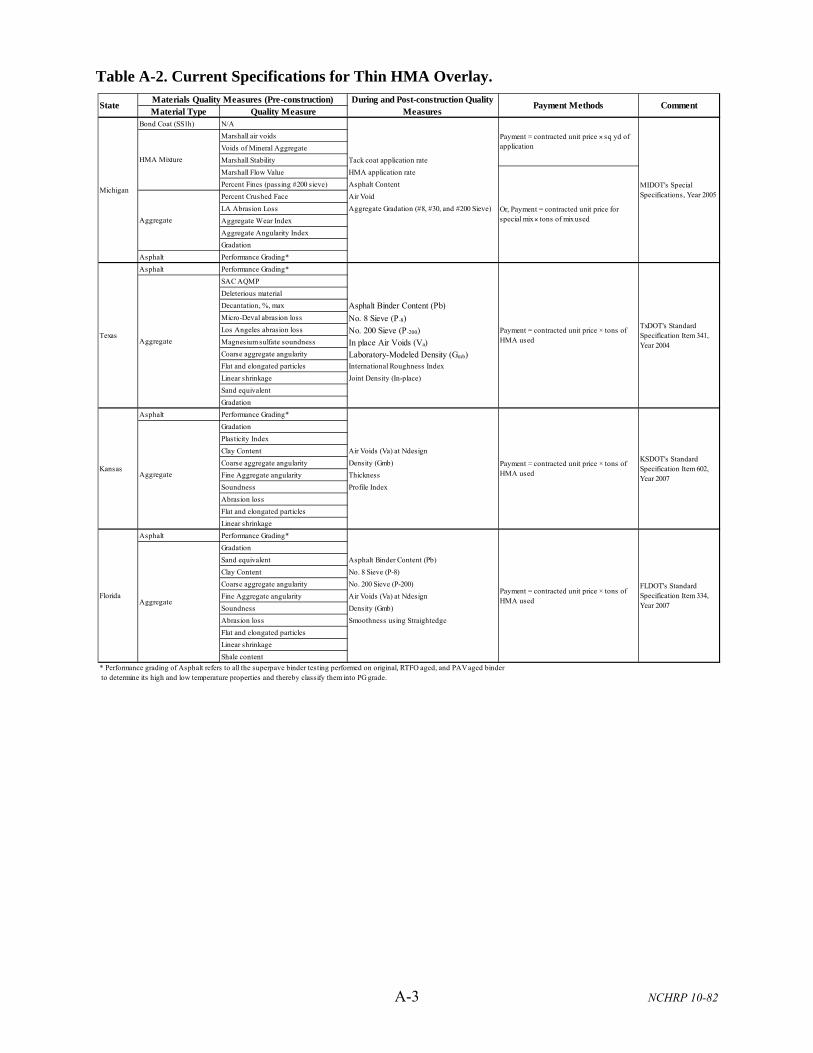
A-3 NCHRP 10-82

Table A-2. Current Specifications for Thin HMA Overlay.

Material Type Quality MeasureBond Coat (SS1h) N/A

Marshall air voids

Voids of Mineral Aggregate

Marshall Stability Tack coat application rate

Marshall Flow Value HMA application rate

Percent Fines (passing #200 sieve) Asphalt Content

Percent Crushed Face Air Void

LA Abrasion Loss Aggregate Gradation (#8, #30, and #200 Sieve)

Aggregate Wear Index

Aggregate Angularity Index

Gradation

Asphalt Performance Grading*


SAC AQMP

Deleterious material

Decantation, %, max Asphalt Binder Content (Pb)Micro-Deval abrasion loss No. 8 Sieve (P-8)Los Angeles abrasion loss No. 200 Sieve (P-200)Magnesium sulfate soundness In place Air Voids (Va)Coarse aggregate angularity Laboratory-Modeled Density (Gmb)Flat and elongated particles International Roughness Index

Linear shrinkage Joint Density (In-place)

Sand equivalent

Gradation


Gradation

Plasticity Index

Clay Content Air Voids (Va) at Ndesign

Coarse aggregate angularity Density (Gmb)

Fine Aggregate angularity Thickness

Soundness Profile Index

Abrasion loss

Flat and elongated particles

Linear shrinkage


Gradation

Sand equivalent Asphalt Binder Content (Pb)

Clay Content No. 8 Sieve (P-8)

Coarse aggregate angularity No. 200 Sieve (P-200)

Fine Aggregate angularity Air Voids (Va) at Ndesign

Soundness Density (Gmb)

Abrasion loss Smoothness using Straightedge

Flat and elongated particles

Linear shrinkage

Shale content

* Performance grading of Asphalt refers to all the superpave binder testing performed on original, RTFO aged, and PAV aged binder to determine its high and low temperature properties and thereby classify them into PG grade.

FLDOT's Standard Specification Item 334, Year 2007

FloridaAggregate

Payment = contracted unit price × tons of HMA used

KansasAggregate

Payment = contracted unit price × sq yd of application

HMA Mixture

Aggregate


KSDOT's Standard Specification Item 602, Year 2007


TxDOT's Standard Specification Item 341, Year 2004

CommentMaterials Quality Measures (Pre-construction)

StateDuring and Post-construction Quality

MeasuresPayment Methods

TexasAggregate

MichiganMIDOT's Special Specifications, Year 2005

Or, Payment = contracted unit price for special mix × tons of mix used

A-4 NCHRP 10-82

Table A-3. Current Specifications for HMA Cold-in-Place Recycling.

Material Type Quality MeasureViscosityResidue percentage from distillationPenetration Pulverizing size (below 1.5 inch)Ductility of residue Emulsified binder agent percentageFloat (residue's ability to flow at high temp) Number of roller passElastic Recovery (on residue) Smoothness using straightedge (longitudinal Sieve Test (% particle larger than certain sieve

Recycled Asphalt Pavement Moisture Content of combined mixViscosityPenetrationSieve Test (% particle larger than certain sieve Float (residue's ability to flow at high temp)Coating Ability and water resistanceStorage StabilityGradationActive Lime content Pulverizing size (below 1.0 inch)Surface Aggregate Classification Cross Slope Smoothness using straightedgeMicro-Deval Abrasion Loss Depth of PlanningMagnesium Sulphate SoundnessMixture DesignMoisture Content of combined mixEmulsion contentGradation of Pulverized pavementHamburg Wheel Tracking TestingIndirect Tensile StrengthCompacted DensityPerformance GradingSieve Test (% particle larger than certain sieve Viscosity Asphalt stabilizing agent application ratePenetration (on residue Depth of PlanningStorage Stability Profile IndexGradation Cross Slope PercentageMixture Design Cross Slope PercentageDensityMoisture ContentMixture DesignGradationLA Abrasion LossFreeze Thaw Loss Pulverizing size (below 2.0 inch)Crushed particle percentage Thickness of compacted layerFlat & Elongated Particle Smoothness using straightedge (longitudinal Magnesium Sulphate Soundness

Additive (if any) N/ABituminous Material N/A

ViscositySieve Test (% particle larger than certain sieve Settlement percent (5 days)Storage StabilityPenetration (on residue)Residue (percent) Smoothness using straightedge (longitudinal Demuslsibility Application rate of Bituminous MaterialsDuctility (on reside)GradationPlasticity IndexAbrasion LossClay contentCrushed particle percentage

Recycled Asphalt Pavement N/A

Materials Quality Measures (Pre-construction)State

During and Post-construction Quality Measures


Iowa

Asphalt Stabilizing Agent (HFMS-2s, CSS-1, or Foamed asphalt using PG binder)

Recycled Asphalt Pavement

Recycled or combined Asphalt Pavement

Aggregate (if any)New York

TxDOT's Special Specification Item 3209, Year 2010

AZDOT's Special Specification Item 408COREC, Year 2006

Pay = unit price of treatment × sq yd of treatment + unit price bituminous material × gal used + unit price of aggregate × tons used

MTDOT's Standard Specification Section 406, Year 2006

Aggregate (if any)

Recycled or Combined Asphaltic Mixture

Emulsion

IADOT's Standard Specification Item 2318, Year 2010

Payment = Unit bid price of recycling × Sq yd of treatment + unit bid price × Tons of emulsified asphalt

NYDOT's Special Specification Item 405.0201-02 M , Year 2009

Texas

Additive (Lime)

ArizonaEmulsified Binder Agent

Payment = Unit bid price of recycling × Sq yd of treatment + unit bid price × Tons of emulsified asphalt

Montana

Bituminous Material

Aggregate (if any)

Payment = Unit bid price of recycling × Sq yd of treatment + unit bid price × Tons of emulsified asphalt + Unit bid price × cu yd of aggregate

Pay = unit price of treatment × sq yd of treatment + unit price bituminous material × gal used + unit price of aggregate × tons used

A-5 NCHRP 10-82

Table A-4. Current Specifications for HMA Hot-in-Place Recycling.

Table A-5. Current Specifications for Slurry Seal.

Material Type Quality MeasureViscocisitySieve Test (Percentage of particle larger than ceratin Residue percent by evaporation Placement of longitudinal jointFlash point temperature Ride Quality

Virgin Hot Mix Asphalt (if Mixture DesignSurface Course Materials N/A

Surface Course Materials N/A Depth of ScarificationHot Mix Asphalt (overlay) Mixture Design Construction Joint locationSurface Course Materials Penetration grade of extracted binder from existing Recycling Agent N/A Construction Joint locationVirgin HMA Mixture Design Percentage of Virgin HMA

Penetration grade of extracted binder from combined Application Rate of Recycling Determination of lab compacted density

ViscosityResidue percentage from distillationPenetrationDuctility of residue Depth of ScarificationFloat (residue's ability to flow at high temp) Application Rate of Recycling Elastic Recovery (on residue) Percentage of Virgin HMASieve Test (% particle larger than certain sieve size)

Surface Course Materials N/AVirgin HMA Mixture DesignCombined HMA N/A


Payment Methods CommentStateMaterials Quality Measures (Pre-construction)

IowaIADOT's Standard Specification 2309, Year 2010

Payment = Unit bid price × sq yd of treatment + Unit bid price × tons of

New York

Pay = unit price of hot-in-place recycle area of treatment + unit price virgin HMA × tons used

NYDOT's Special Specification Item Item 402.607201-02, Year 2009

TxDOT's Standard Specification 358, Year 2004

TexasRecycling Agent


Combined HMA

Arizona

Recycling AgentAZDOT's Special Specification for Hot-in-Place Recling, Year 2006

Pay = unit price of hot-in-place recycle area of treatment + unit price virgin HMA × tons used + Unit price of recycling agent × tons used

Material Type Quality MeasureViscosity @ 25⁰C and/or 50⁰C

Settlement percent (5 days)

Storage Stability Test, 1day, %

Sieve Test, %

Demuslsibility, 35 ml, 0.02 N CaCl2, %

Coating Ability and Water Resistance

Particle charge test (for cationic asphalt emulsion and polymer modified asphalt emulsion)

Cement mixing test, %

Residue by distillation, %

Ash content (for polymer modified asphalt emulsion only)

Residue by evaporation, % Slurry spread rate (lb/sq.yd)

Penetration (on residue) @ 25⁰C

Ductility (on reside), 50mm/min, mm

Solubility in trichloroethylene (on residue), %

Gradation

Sand Equivalent

Durability Index

Slurry seal consistency, mm

Wet stripping

Compatibility

Cohesion test, kg-mm within one h

Wet track abrasion, g/m2

Viscosity @ 77⁰F

Residue by evaporation, %

Sieve Test, % retained on #20

Particle Charge, Electroplate

Penetration (on residue) @ 77⁰F

Solubility in trichloroethylene (on residue), %

Ductility (on reside) @ 77⁰F, cm Slurry spread rate (lb/sq.yd)

Gradation

Sand Equivalent (minimum 45)

Abration Loss (maximum 75 gm per sq ft)

Slurry Seal Mixing Test, sec

Slurry Seal Setting Test

Slurry Seal Water Resistance Test

Sieve Test

Aggregate Compatibility

Absolute Viscosity

Asphalt Binder Content

Gradation Mix Consistency

Abrasion, maximum

Alumina, maximum

Sand Equivalence, minimum

Organic Materials, maximum

StateMaterials Quality Measures (Pre-construction) During and Post-

construction Quality Payment Methods Comment

AZ

Asphalt Emulsion (QS-h)

Payment = unit bid price × sq yd of slurry seal


Fine Aggregate

IA

Aspahlt Emulsion (CSS-1h or SS-1h)

CA

Aspahlt Emulsion (QS1h, or CQS1h)

Mix Design

Payment = Contracted unit price × tons of slurry seal materials (asphaltic emulsion + aggregate)

CalTran's Standard Specifications Item 37, Year 2006

Fine Aggregate

Payment = unit bid price × gallon of emulsion + unit bid price × tons of aggregate

IOWA DOTs' Standard Specification Item 2319, Year 2010

Aggregate

Mix

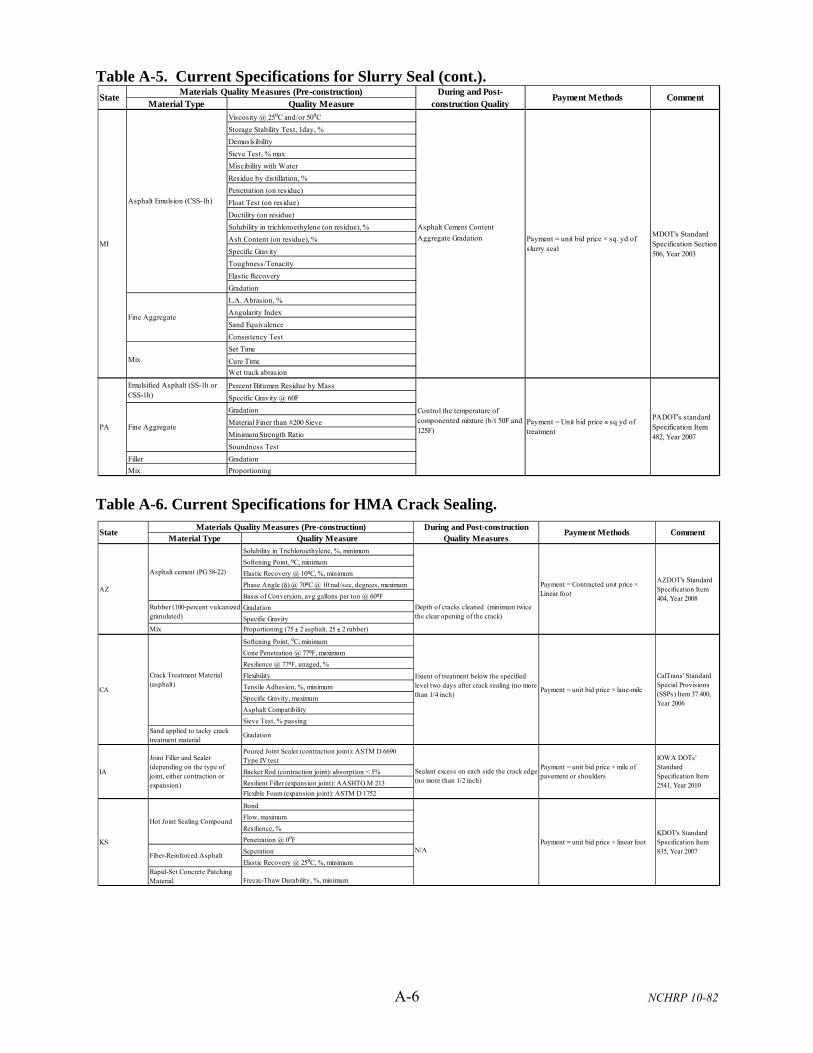
A-6 NCHRP 10-82

Table A-5. Current Specifications for Slurry Seal (cont.).

Table A-6. Current Specifications for HMA Crack Sealing.

Material Type Quality MeasureViscosity @ 25⁰C and/or 50⁰C

Storage Stability Test, 1day, %

Demuslsibility

Sieve Test, % max

Miscibility with Water

Residue by distillation, %

Penetration (on residue)

Float Test (on residue)

Ductility (on residue)

Solubility in trichloroethylene (on residue), % Asphalt Cement Content

Ash Content (on residue), % Aggregate Gradation

Specific Gravity

Toughness/Tenacity

Elastic Recovery

Gradation

L.A. Abrasion, %

Angularity Index

Sand Equivalence

Consistency Test

Set Time

Cure Time

Wet track abrasion

Percent Bitumen Residue by Mass

Specific Gravity @ 60F

Gradation

Material Finer than #200 Sieve

Minimum Strength Ratio

Soundness Test

Filler Gradation

Mix Proportioning

StateMaterials Quality Measures (Pre-construction) During and Post-

construction Quality Payment Methods Comment

Mix

PA

Emulsified Asphalt (SS-1h or CSS-1h)

Fine Aggregate

MI

Asphalt Emulsion (CSS-1h)


PADOT's standard Specification Item 482, Year 2007

Control the temperature of componented mixture (b/t 50F and 125F)

Payment = unit bid price × sq. yd of slurry seal

MDOT's Standard Specification Section 506, Year 2003

Fine Aggregate

Material Type Quality MeasureSolubility in Trichloroethylene, %, minimum

Softening Point, ⁰C, minimum

Elastic Recovery @ 10⁰C, %, minimum

Phase Angle (δ) @ 70⁰C @ 10 rad/sec, degrees, maximum

Basis of Conversion, avg gallons per ton @ 60⁰F

Gradation

Specific Gravity

Mix Proportioning (75 ± 2 asphalt, 25 ± 2 rubber)


Cone Penetration @ 77⁰F, maximum

Resilience @ 77⁰F, unaged, %

Flexibility

Tensile Adhesion, %, minimum

Specific Gravity, maximum

Asphalt Compatibility

Sieve Test, % passing

Sand applied to tacky crack treatment material

Gradation

Poured Joint Sealer (contraction joint): ASTM D 6690 Type IV test

Backer Rod (contraction joint): absorption < 5%

Resilient Filler (expansion joint): AASHTO M 213

Flexible Foam (expansion joint): ASTM D 1752

Bond

Flow, maximum

Resilience, %

Penetration @ 0⁰F

Seperation N/A

Elastic Recovery @ 25⁰C, %, minimumRapid-Set Concrete Patching Material Freeze-Thaw Durability, %, minimum


Quality MeasuresPayment Methods Comment

Fiber-Reinforced Asphalt

Rubber (100-percent vulcanized granulated)

Depth of cracks cleaned (minimum twice the clear opening of the crack)

Crack Treatment Material (asphalt)

Extent of treatment below the specified level two days after crack sealing (no more than 1/4 inch)

Sealant excess on each side the crack edge (no more than 1/2 inch)

KS

Hot Joint Sealing Compound

Payment = unit bid price × linear footKDOT's Standard Specification Item 835, Year 2007

CA Payment = unit bid price × lane-mile

CalTrans' Standard Special Provisions (SSPs) Item 37.400, Year 2006

IA

Joint Filler and Sealer (depending on the type of joint, either contraction or expansion)

Payment = unit bid price × mile of pavement or shoulders

IOWA DOTs' Standard Specification Item 2541, Year 2010

AZ

Asphalt cement (PG 58-22)

Payment = Contracted unit price × Linear foot


A-7 NCHRP 10-82

Table A-6. Current Specifications for HMA Crack Sealing (cont.).

Material Type Quality MeasureBond

Flow, maximum

Resilience, %

Penetration @ 0⁰F

Seperation N/A

Elastic Recovery @ 25⁰C, %, minimumRapid-Set Concrete Patching Material Freeze-Thaw Durability, %, minimum

Penetration @ 25 ⁰C


Viscosity @ 60⁰C (on aged residue)

Length

Crimps Adhesion failure

Tensile Strength Cohesion failure

Denier Missed crack

Specific Gravity

Melting Temperature

Ignition Temperature

Cone Penetration @ 77F

Cone Penetration @ 0F, min

Flow @ 60⁰C, maximum

Resilience @ 77⁰F, %

Bond @ 20F N/A

Recommended Pour Temperature

Safe Heating Temperature


Backer Rod ASTM D-5249, Type 1

Tensiel Stress at 150% Elongation, psi, max

Elongation at Maximum Tensile Strength, %, min

Extrusion Rate, grams/second, min

Specific Gravity

Durometer Hardness

Shelf Life, days, min

Ozone and Ultraviolet Resistance

Flow

Bond to Cement Mortar, psi, min N/A

Tack Free Time, minutes, max

Movement Capability and Adhesion

Cone Penetration @ 77⁰F

Flow @ 60⁰C, maximum

Resilience @ 77⁰F, unaged, %

Ductility @ 77F, maximum

Bond, non-immersed @ 0F

Asphalt Compatibility @ 140F

Sealant Life at Application Temperature, minimum

Penetration @ 77F

Bond at -20F N/A

3 Cycles, 200% Extension

Unit Weight, lbs/gal (no greater than 9.36)

Rotational Viscosity

Sieve Test

Storage Stability

Residue by Evaporation

Penetration (on residue)

Softening Point (on residue)

Ductility (on residue)

Crumb Rubber Modifier (CRM) Content, Grade A or B N/A

Virgin Rubber Content

Flash Point

Penetration

Softening Point

Bond

Cone Penetration, 130 max

Softening Point

ResilienceBond N/A


Minimum Application Temperature

Maximum Heating Temperature



Payment = Unit bid price × foot, gallon, pound, or lane mile

TxDOT's Standard Specification Item 712, Year 2004

Polyester Fibers

Fiber-Reinforced Asphalt

Ruberized Joint Sealing Material

WA Payment = unit bid price × linear foot

TX

MTCrack Sealant

SealantPayment =unit bid price × pound (kg) of sealant used

SDDOT's Standard Specification Item 350, Year 2004

WSDOT's Standard Specification Item 9-04.10, Year 2010

Polymer Modified Asphalt Emulsion

Payment = Unit bid price × pound (kg) of material placed

MTDOT's standard Specification Item 403, Year 2006

Rubberized Asphalt

Rubber-Asphalt Crack Sealer

PA

Asphalt Rubber Sealing Compound

Payment = unit bid price × linear footPADOT's Standard Specification Item 469, Year 2008

SD

KS

Hot Joint Sealing Compound

Payment = unit bid price × linear footKDOT's Standard Specification Item 835, Year 2007

MI

Polymer Modified Asphalt Cement

Payment = unit bid price × roadbed mileMDOT's Standard Specification Section 505, Year 2003

A-8 NCHRP 10-82

Table A-7. Current Specifications for PCC Joint Resealing and Crack Sealing.

Material Type Quality MeasureJoint sealant and filler N/ABacker Rod

Cleveland Open Cup Flash PointCone PenetrationViscosityCuring TimeBond StrengthDurometer Hardness

Asphalt Filler

When a strip 2-inches wide and 24-inches long is freely supported 2-inches from each end and maintained at 70°F, it shall support a weight of 100 grams placed at the center of the strip without deflecting downward from a horizontal position more than 2-inches within a period of 5 minutes

cone penetrationFlowBond StrengthResilience Tensile StressElongationDurometer HardnessBond StrengthTack free timeTensile StressElongationDurometer HardnessBond StrengthCone PenetrationFlowResilience RecoveryBond Strength

Backer Rod N/ASand GradationEpoxy-resin to Sand ratio

hot poured joint sealerelastomeric joint sealsHot-Poured Joint SealantBacker Rod

New York Silicone Joint Sealant Payment = Unit bid price × linear ft of joints sealed

NYDOT's special specification ITEM 18502.701002 M, Year 1996

Tensile StressElongationBond StrengthDurometer HardnessCone PenetrationResilience RecoverySoftening Point

Backer RodLow Modulus Silicone Sealant:Hot-Poured Type Sealant

Texas

PADOT's Standard Specification Section 513, Year 2007

SDDOT's standard specification Item 390

Payment = Unit bid price × linear ft of joints sealed

Special Specification 7435, Year 2004

WADOT's standard specification 5-01, 2010


Washington

Poured Rubber Joint Sealer

Hot poured Joint Sealant

Height of sealant in jointPayment = Unit bid price × linear ft of joints sealed

South Dakota

Hot Poured Elastic Joint Sealer

Low Modulus Silicone Sealant:

Arizona DOT's Specification for Joint and Crack Resealing Section 402-6


Height of sealant in jointJoint Sealant MaterialsArizona

Payment = Unit bid price for clean and seal joints and crack × linear ft of crack and

Pennsylvania

Joint Sealant

Rubberized Joint Sealing Materials

Iowa


Michigan DOT's Standard Specification Item 603, Year 2003

Height of sealant in jointMichigan

FloridaPayment = Unit bid price × linear ft of joints sealed

FDOT's Standard Specification Item 350-12.7, Year 2010

California

Silicone Joint Sealant

Asphalt Rubber Joint Sealant




CalTrans' Standard Special Provision 41-210, Year 2007

Failure of the joint material in either adhesion or cohesion of the material will be cause for rejection.

Sealant dimension in the jointPayment = Unit bid price for sealer material × lb of sealer + unit bid price fro cleaning

Iowa DOT's Standard Specification Section 2542, Year 2010

A-9 NCHRP 10-82

Table A-8. Current Specifications for PCC Partial-Depth Repair.

Material Type Quality MeasureFlexural Strength Test in 5 hrCompressive Strength test at 7 days and 28 daysShrinkage Test

Polymeric Patch Materials N/APayment = Unit Bid Price × Gallons of Polymeric Patch Material

Compressive Strength (3 hr and 24 hr)Bonding StrengthShrinkage TestSet timeAir contentCompressive Strength

Hot mix asphalt (HMA) N/APayment = Unit Bid Price X Area of Patch + Unit price × Weight of HMA Patch Material

Bonding Mortar for Concrete Patches

N/APayment = Unit Bid Price for Saw and Seal × Length of Joints Repaired

Concrete Patches Air content Payment = Unit bid price for Type A spall repair × square ft spall repaired

Epoxy Resin Mortar N/ASilicone Sealant N/AType 1 repair with Class AA Cement Concrete, Modified.

Compressive StrengthPayment = Unit bid price for saw and seal × length of joints repaired

Type 2 repair with Class AA Cement Concrete, Special.

N/A

Type 3 repair with Rapid Set Concrete Patching Materials.

N/A

Type 4 repair with Latex Modified Concrete.

N/A

Type 5 repair with Thin Bonded Portland Cement Concrete Inlay

N/A

Compressive StrengthAir ContentMoisture content of aggregate

Concrete Repair Material or Rapid Hardening Concrete Repair Material

N/A

Rapid Hardening Polymer Concrete.

N/A

Epoxy Resin System N/AAccelerated Strength Port land Cement Concrete Patch Material

Compressive strength test (6 hr)

Rapid Setting Patch Materials

compressive strength (6 hr)

Epoxy Resin Grout Patch Material

epoxy binder to aggregate ratio

Tensile StrengthTensile ElongationTensile Bond StrengthHardnessCement ContentAir Content (5.5±1.5%)Flexural Strength (at traffic opening time)Compressive Strength (3 hr and 24 hr)Flexural StrengthBond StrengthDrying ShrinkageSetting timeTensile StrengthElongationBond StrengthDurometer Hardness

Repair of Spalling Item 720, Year 2004


AZDOT's Standard Specification Item 402-2, Year 2008

NYDOT's Item 502.46010018 Partial-Depth Repair using epoxy resin, Year 2003

Iowa

Minimum depth of patching saw cutSounding (pre-repair) and Resounding (post-repair) Test

SDDOT's Standard Specification Item 390, "Concrete Spall Repair", Year 2004

Portland cement concrete patching material

South Dakota

Iowa DOT’s specifications Partial Depth Repair (Item 2530 ), Year 2010

PADOT's Standard Specification Section 525 for Concrete Spall Repair, Year 2007

Minimum depth of patching saw cutResounding test

New York

NYDOT's Item 502.4MR00018 Partial-Depth Repairs, Year 2003

Minimum and maximum saw cut depth

Payment = Unit bid price for spall repair × square ft spall repaired

Texas

Washington Concrete patching material NA

Flexible Epoxy Patching Material

Minimum depth of patching saw cut

Concrete Patch Materials

Payment = Unit bid price for pavement repair × square yard of area repaired

Michigan Patching Concrete Smoothness test using straight edge


Fast-Setting Grout


California Minimum saw cut depth for patching


Payment = Unit bid price for pavement repair × square yard of area repaired

Comment

Minimum saw cut depth for patching


Payment = Unit Bid Price × Cubic ft of Concrete Patch Material


Quality MeasuresPayment Methods

Payment = Unit bid price for spall repair × square ft spall repaired


ArizonaPayment = Unit bid price for spall repair × square ft spall repaired

Pennsylvania

Payment = Unit Bid Price X Area of Patch

Payment = Unit bid price for Type B spall repair × length of spall repaired

Transit Mix High Early Strength Concrete.

A-10 NCHRP 10-82

Table A-9. Current Specifications for PCC Full-Depth Repair.

Material Type Quality MeasureFlexural Strength Compressive StrengthYield StrengthPullout Strength

Asphalt Concrete N/ACompressive Strength (3 hr, 24 hr)Shrinkage Placement of dowel and tie barFreeze-Thaw Smoothness using straight edgeBond Strength Placement of dowel and tie barAir Content Profile Index Compressive Strength

Compressive Strength (7 hr, 28 day)Air Content Ride acceptance using straight edge

Reinforcement. N/A Compressive Strength before opening to Dowels N/AAccelerated Strength Concrete Compressive Strength (6 hr)Tie bar Yield StrengthJoint sealant Yield Strength

Cement ContentAir Content (5.5±1.5%)Flexural Strength (at traffic opening

Reinforcement. N/ADowel bar N/A

Compressive Strength at 6 hr and 24 Smoothness test using 10 ft straight edge, Air Content (1 to 6%) Maturity Method Testing before opening to

Rapid Strength Concrete Modulus of Rupture Strength (7 day)Contraction in airMortar expansion in water Smoothness test using straight edgeSoluble chloride Co-efficient of FrictionSoluble sulfates Groove dimensionThermal stabilityCompressive strength @ 3 days

Hot mix Asphalt Asphalt Content

Air Content Patch thicknessCement Content Smoothness of patch using straightedge Payment = Unit bid price × sq yd of

Hot mix Asphalt N/A Core density (HMA) Payment = Unit bid price × tons of Dowel bar and tie bar N/A Profile Index (for patch longer than 50 ft)


MichiganPatching Concrete

Smoothness test using straight edgePayment = Unit Bid price × sq yd of repaired surface area + (price for additional items)

PennsylvaniaPADOT's Standard Specification Item 516, Year 2007

Arizona Depth of patchPayment = Unit Bid price × sq yd of repaired surface area


MeasuresPayment Methods Comment

Materials Quality Measures (Pre-construction)

Hydraulic Cement Concrete

Reinforcement.

Concrete patching material

Portland Cement Concrete

Payment = unit bid price × corresponding items measured

IowaPortland Cement Concrete

FLDOT's Standard Specification Section 353,

WashingtonPayment = Unit Bid price × sq yd of repaired surface area


Florida Portland Cement ConcretePayment = Unit Bid price × Cu yd of concrete placed

AZDOT's Standard Specification Item 402-3, Year 2008

TexasPayment = Unit Bid price × sq yd of repaired surface area

TxDOT's Item 361, Year 2004

Cement Concrete Class AA

IADOT’s specifications Full Depth Finish Patch (Item 2529 ), Year 2010

CaliforniaPayment = Unit Bid price × Cu yd of concrete placed


Hydraulic Cement

A-11 NCHRP 10-82

Table A-10. Current Specifications for Load Transfer Restoration (Dowel Bar Retrofitting).

Material Type Quality MeasureDowel Bar Tensile StrengthEpoxy resin Epoxy resin to sand ratio

Yield Strength Positioning of Dowel Bar,

Epoxy coating thicknessCompressive Strength of patching material

Rapid Set Concrete Patching Material

Shelf life

Dowel Bar N/ACompressive Strength (3 hr and 24 hr)Final Set time Positioning of Dowel BarFlexural Strength (if aggregate added)

Compressive Strength (6 hr, 24 hr)

Bond Strength

Tensile StrengthEstimate Concrete Strength by Maturity MethodCompressive Strength of patching material

Class HES Concrete Compressive Strength Positioning of Dowel BarCompressive Strength (3 hr and 24 hr)ShrinkageBond StrengthFreeze-Thaw LossThickness of epoxy coatingTensile StrengthYield StrengthCorrosion AbrasionLoad DeflectionPull-OutCompressive Strength (3 hr and 24 hr)ShrinkageFreeze-Thaw LossBond Strength

Joint Forming Materials DimensionTensile Strength (yield)Thickness of epoxy coating

Concrete patching material N/ADowel Bar N/ABond Breaker N/A

Compressive Strength (3 hr and 24 hr)Flexural Strength Saw cut depth within certain tolerance

Bond StrengthPlacement of dowel bar within certain tolerance

Drying Shrinkage Verification of grinding on grouted area

Setting timeVerification of dowel bar positioning by coring

Tensile StrengthElongationBond StrengthDurometer Hardness

Positioning of Dowel BarPayment = unit bid price × number of dowel bar retrofitted

Positioning of Dowel Bar

PennsylvaniaPayment = unit bid price × number of dowel bar installed

PADOT's Standard Specification Item 527, Year 2007

MIDOT's Special Provision for Dowel Bar Retrofit, Year 2000

MichiganDowel Bar Payment = unit bid price × number

of dowel bar retrofitted

WA DOT's Specification for Dowel Bar Retrofit (Section 5-01), Year 2010


ArizonaPayment = unit bid price × ft of joint repair

AZ DOT's Standard Specification (Section 402-6-C)

Payment = unit bid price × number of dowel bar installed

TxDOT's Special Specification 3012, Year 2004


Dowel bar

CaliforniaFast Setting Grout


Payment = unit bid price × number of dowel bar retrofitted

South DakotaPayment = unit bid price × number of dowel bar installed

Texas

Washington

Backfill Materials (Patching materials)

Retrofit LTDs (Dowel Bar)


Dowel Bar

Materials Quality Measures (Pre-construction) During and Post-construction Quality Measures

Payment Methods CommentState

New YorkPayment = unit bid price × number of dowel bar retrofitted

Positioning of Dowel Bar

SDDOT’s Special Provision for PPCP Dowel Bar Retrofit, Year 2001

NYDOT,s Special Specification Item 502.70010018, Year 2003

A-12 NCHRP 10-82

Table A-11. Current Specifications for PCC Diamond Grinding.

Table A-12. Current Specifications for PCC Slab Stabilization (Undersealing).

Material TypeQuality

MeasureGroove DimensionProfile IndexPercentage of ground areaMinimum Coefficient of frictionUniformity of transverse slopeProfile IndexMinimum Coefficient of frictionSmoothness Test using straight edgeProfile IndexProfile IndexHeight of individual bumpUniformity of transverse slopePercentage of ground areaPercentage of ground areaSmoothness Test using straight edgeDimension of GrooveFaulting height near transverse cracksPercentage of ground areaProfile IndexProfile IndexHeight Individual BumpGroove DimensionProfile IndexPercentage of ground areaGroove DimensionProfile IndexSmoothness Test using straight edgeGroove depth and spacingUniformity of cross slope (Transverse direction)Roughness test in longitudinal direction (IRI)

Payment = Unit bid price × square yard of treatment

California N/APayment = Unit bid price × square yard of treatment

California Standard Specification (Section 42-2) Year 2006

Arizona N/APayment = Unit bid price × square yard of treatment

Payment = Unit bid price × square yard of treatment

Michigan Standard Specification (Section 603.03) Year 2003

Iowa

Florida Standard Specification (Section 352) Year 2010

Florida N/A

New York N/APayment = Unit bid price × square yard of treatment

New York's Specification for Diamond Grinding (Special Item 502.81010018

Michigan N/A

South Dakota's Specification for Diamond Grinding (Special Provision

Texas N/APayment = Unit bid price × square yard of treatment

Texas' Special Specification (Special Specification 3088)

Washington N/APayment = Unit bid price × square yard of treatment

Washington State DOT's Specification (Item 5-01.3(9)) Year 2010

N/A

N/A

N/A

South Dakota

N/APayment = Unit bid price × square yard of treatment

PADOT's Specification for Diamond Grinding (Item 514) Year 2007

Payment = Unit bid price × square meter of ground area


MeasuresPayment Methods

N/A

N/A

N/A

N/A

Pennsylvania

CommentMaterials Quality Measures

N/A

N/A

N/A

N/AIowa Special Specification (Section 2532) Year 2010

N/APayment = Unit bid price × square yard of treatment

Arizona Standard Specification (Section 402-4) Year 2008

Material Type Quality Measure

Expansion TestMaximum upward movement of the slab

Initial setting time SmoothnessCompressive Strength (7 day) Deflection Test

Efflux TimeMaximum upward movement of the slab

Initial setting time Deflection TestCompressive Strength (7 day)

Efflux TimeMaximum upward movement of the slab

Compressive Strength (7 day) Deflection Test

New York Grout SlurryPayment = unit bid price × cubic meter of grout filling

New York's special specification Item 01501.12 M, Year 1997

Set TimeCompressive StrengthEfflux Time

Materials Quality Measures (Pre-construction)State



Pennsylvania

Payment = unit price of cement × weight of cement + unit price of drill hole × no of holes + unit price of deflection testing × no of testing

PADOT’s specifications for Concrete Pavement Slab Stabilization Item 679, Year 2007

Grout Slurry

TexasPayment = unit price of grout slurry × cubic ft of cement or fly ash + unit price of drilled hole × no of holes

TxDOT's Special specification 3004: pressure Grouting, Year 2004

Maximum upward movement of the slab

South Dakota

Payment = unit price of cement × cubic ft of cement + unit price of drill hole × no of holes + unit price of deflection testing × no of testing

South Dakota's Item 391, Year 2004

Iowa

Grout Slurry

Grout Slurry

California Grout SlurryMaximum allowable upward movement of the slab

Payment = unit bid price × no of holes + unit bid price for grout × weight of cement or fly ash

CalTrans' Standard Specification 41-1, Year 2006

Payment = unit price of cement × ton of cement + unit price of drill hole × no of holes filled + 50% of unit price of drilled holes × no of inspection holes

Efflux TimeGrout SlurryIowa's Standard Specification Section 2539, Year 2010

B-1 NCHRP 10-82

Appendix B. Bibliography of Current Pavement Performance Prediction Models

PERFORMANCE MODELS FOR HMA PAVEMENT TREATMENTS An extensive literature review has been conducted by the research team to search for existing pavement preservation performance prediction models. It was found that significant efforts had been put into developing promising prediction models for HMA pavement preservations. Though some of the efforts have proposed rational performance prediction models, none of them has the ability correlating initial materials and construction properties with future performance of preservation treatments. A summary of reviewed performance prediction models for HMA pavement preservations is presented below. Figure B-1 graphically shows potential influential factors that have an important effect on preservation treatment performance. These factors are categorized into four groups, materials-related, construction-related, traffic-related, and environment-related.

Figure B-1. Influential Factors on HMA Pavement Preservation Treatments

Influential Factors

Materials

Asphalt binder

Type

Content

Demulsibility

Penetration

% asphalt residue

Viscosity

AggregateType

Gradation

Mineral filler (if applciable)

Type

% filler

Polymer (if applicable)

MixtureAir voids

Thickness

Construction

Surface preparation

Asphalt application rate

Aggregate application rate

Temperature

Rolling

CuringTraffic

AADT

%Truck

Traffic growth factor

EnvironmentFreeze Index

Annual precipitation

B-2 NCHRP 10-82

Morian, Gibson, and Epps, 1998

Morian et al. (1998) performed a 5-year study using the long-term pavement performance (LTPP) data. Linear regression models were developed for predicting the pavement rating score (PRS) as a function of a group of traffic, environment, and site-specific variables. PRS is a composite 0-100 scale performance indicator, computed based upon distress conditions including fatigue cracking, longitudinal cracking, transverse cracking, and patching. Regression models were developed for thin overlay, slurry seals, crack seals, and chip seals, having the following forms:

Thin Overlay: 43.3476 1.88071 6.137 4.37 6.122( )PRS EZ Age IC SG

Slurry Seal: 23.426 4.42829 6.92985 6.92985PRS EZ Age IC

Crack Seal: 26.7872 6.54727 11.23PRS EZ IC

Chip Seal: 45.26 4.37 9.79 9.21( ) 10.43( )PRS Age IC SA SG

where, EZ = Environmental zone (dry-no freeze, dry-freeze, wet-no freeze, wet-freeze), Age = Year of pavement preservation treatment, IC = Original pavement condition level (good, fair, and poor), SA = Pavement structural adequacy (structural number ratio either greater than or less

than one), SG = Subgrade type (fine verses coarse).

Hajek and Bradbury, 1999

The Canadian Strategic Highway Research Program (C-SHRP) employed Bayesian statistical analysis methodology for modeling pavement deterioration (Hajek and Bradbury 1999). In this application, distress prediction models were first constructed based on data alone using linear regression. The researchers then selected the best models for further analysis, in which experts with extensive experience in pavement were requested to rate the level of distress at different age with different traffic and asphalt content using a 0-to-10 scale. Based on experts input, prior models were developed using the C-SHRP Bayesian analysis software, and then posterior models were developed from the prior models and field data using “N-prior” analysis option built in the analysis software. Final distress prediction model was selected based on sensitivity analysis. The final model has the following form:

DI = 127 + 5.64(Age) - 18.5(AC) - 5.88log(Traffic) Where,

DI = Distress index, Age = Age of the pavement surface course, AC = Design percentage by mass of asphalt cement content in the surface course, Traffic = AADT volume per lane.

Eltahan, Daleiden, and Simpson, 1999

Eltahan et al. (1999) employed the Kaplan-Meier method to develop a model that predicts the probability of treatment failure at a given time as expressed in the following form.

1 ( 1)

( ) 1( 1) 1 1r

n n r n rF t

n n r n r

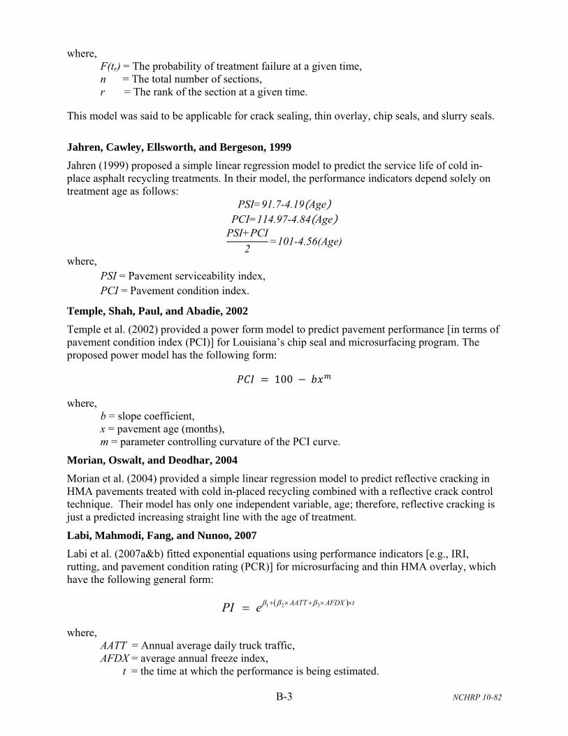
B-3 NCHRP 10-82

where, F(tr) = The probability of treatment failure at a given time, n = The total number of sections, r = The rank of the section at a given time.

This model was said to be applicable for crack sealing, thin overlay, chip seals, and slurry seals.

Jahren, Cawley, Ellsworth, and Bergeson, 1999

Jahren (1999) proposed a simple linear regression model to predict the service life of cold in-place asphalt recycling treatments. In their model, the performance indicators depend solely on treatment age as follows:

PSI=91.7-4.19 Age

PCI=114.97-4.84 Age PSI+PCI

2=101-4.56(Age)

where, PSI = Pavement serviceability index, PCI = Pavement condition index.

Temple, Shah, Paul, and Abadie, 2002

Temple et al. (2002) provided a power form model to predict pavement performance [in terms of pavement condition index (PCI)] for Louisiana’s chip seal and microsurfacing program. The proposed power model has the following form:

100

where, b = slope coefficient, x = pavement age (months), m = parameter controlling curvature of the PCI curve.

Morian, Oswalt, and Deodhar, 2004

Morian et al. (2004) provided a simple linear regression model to predict reflective cracking in HMA pavements treated with cold in-placed recycling combined with a reflective crack control technique. Their model has only one independent variable, age; therefore, reflective cracking is just a predicted increasing straight line with the age of treatment.

Labi, Mahmodi, Fang, and Nunoo, 2007

Labi et al. (2007a&b) fitted exponential equations using performance indicators [e.g., IRI, rutting, and pavement condition rating (PCR)] for microsurfacing and thin HMA overlay, which have the following general form:

1 2 3 AATT AFDX tPI e

where, AATT = Annual average daily truck traffic, AFDX = average annual freeze index, t = the time at which the performance is being estimated.

B-4 NCHRP 10-82

Liu, Hossain, and Miller, 2009

Liu et al. (2009) proposed linear models predicting distresses development on HMA pavements treated with chip seals. The covered distresses included IRI, rutting, transverse cracking, and fatigue cracking. These linear models are summarized as follows:

Roughness: IRI=3.97091+0.89323 InitIRI +2.87797 Age +1.29244(FC)

Rutting: RUT=0.03621+0.76501 InitRUT -0.00404(FC)

Transverse Cracking: TCR=-0.0765+0.7833 InitTCR +0.0175 Age +0.0561(FC)

Fatigue Cracking: FCR=-0.24839+0.49664 InitFCR +0.00008 ESAL +0.15381(FC)

where, InitIRI = First year IRI value after chip-sealing, InitRUT = First year rut depth after chip-sealing, InitTCR = First year transverse crack value after chip-sealing, InitFCR = First year fatigue crack value after chip-sealing, Age = Year of chip seal treatment, FC = Highway functional class (interstate, US, and state highways), ESAL = Cumulative equivalent 18-kip single axle loads.

MEPDG, 2004

The mechanistic-empirical pavement design guide (MEPDG) employs several pavement distress prediction models to estimate distress development in newly constructed or overlaid HMA pavements. The distresses that can be predicted in MEPDG include fatigue cracking (both alligator and longitudinal), thermal cracking (transverse), performance deformation (rutting), and smoothness (IRI).

Fatigue Cracking

In MEPDG the estimation of fatigue damage is based upon Miner’s Law, as following:

1

Ti

i i

nD

N

where, D = damage, T = total number of periods, ni = actual traffic for period i, and Ni = traffic allowed under conditions prevailing in i.

The number of load repetitions to fatigue cracking can be predicted as a function of the tensile strain and mix stiffness (modulus). In MEPDG, the national field calibrated model has the following form:

3.9492 1.281

'1

1 10.00432f

t

N k CE

where, Nf = number of load repetitions to fatigue cracking,

'1k = correction factor for asphalt layer thickness effects,

B-5 NCHRP 10-82

εt = tensile strain at the critical location, E = stiffness of the material,

C = laboratory to field adjustment factor, and4.84 0.69

10b

a b

V

V VC

,

where, Vb = effective binder content (%), and Va = air voids (%).

The “ '1k ” value has different computation forms for bottom-up cracking and top-down cracking:

a. For bottom-up cracking (alligator cracking):

'1

11.02 3.49

10.003602

0.0003981 ach

k

e

b. For top-down cracking (longitudinal cracking):

'1

15.676 2.8186

112.0

0.011 ach

k

e

where, hac = total thickness of the asphalt layers in inch. The '

1k value ranges from 0 to 2,500 for bottom-up cracking and from 0 to 100 for top-down

cracking, as shown in Figure B-2.

Figure B-2. '1k versus hac for Bottom-up and Top-down Cracking

The fatigue damage can then be calculated into fatigue cracking using a transfer function, which has the following forms:

a. For bottom-up cracking (% of total lane area):

' '

1 1 2 2* * *log10 *100

1 6000

60 1bottom up C C C C D

FCe

where,

0 2 4 6 8 10

50

01

00

01

50

02

00

02

50

0

hac

k1'

bottom-up cracking

0 2 4 6 8 10

02

04

06

08

01

00

hac

k1'

top-down cracking

B-6 NCHRP 10-82

FCbottom-up = bottom-up fatigue cracking, percent lane area, D = bottom-up fatigue damage (obtained from Eq. 2), C1 = 1.0,

' '1 22*C C ,

2 1.0C ,

2.856'2 2.40874 39.748 1 acC h

.

b. For top-down cracking (feet/mile):

7.0 3.5*log10 *100

100010.56

1top down D

FCe

where, FCtop-down = top-down fatigue cracking, ft/mile, D = top-down fatigue damage.

Thermal Cracking

In MEPDG, the amount of thermal (transverse) cracking expected in the pavement system is predicted by relating crack depth to the amount of cracking as follows:

1

log /* ac

f

C hC N

where, Cf = observed amount of thermal cracking, β1 = regression coefficient from field calibration, N(z) = standard normal distribution evaluated at (z), σ = standard deviation of the log of the depth of cracks in the pavement, C = crack depth, and hac = thickness of asphalt layer.

Using the Paris Law, the amount of crack propagation induced by a given thermal cooling cycle is predicted by the following expression:

nC A K

where, ΔC = change in the crack depth due to a cooling cycle, ΔK = change in the stress intensity factor due to a cooling cycle, A, n = fracture parameters for the asphalt mixture, which can be derived from the following equations:

1

0.8 1nm

where, m is the slope of the compliance curve.

and

* 4.389 2.52*log * *

10 mE nA

where, E = mixture stiffness,

B-7 NCHRP 10-82

σm = undamaged mixture tensile strength, β = calibration parameter.

Permanent Deformation

In MEPDG pavement permanent deformation is the total rutting in the pavement structure (asphalt surface, granular base/subbase, and subgrade). Thus, the total rutting can be expressed by the following equation:

Total AC GB SGRD RD RD RD

Pavement structure is divided into a number of sublayers. The plastic strain in each sublayer is evaluated, and the overall performance deformation is the accumulation of the product of plastic strain and thickness of individual sublayers as follows.

#

1

of sublayersi ip

i

RD h

where, RD = Pavement permanent deformation,

ip = Total plastic strain in sublayer i, ih = Thickness of sublayer i.

For asphalt mixtures, the plastic strain has the following model form:

3.4488 1.5606 0.4792441 *10p

r

k T N

where,

p = Accumulated plastic strain at N repetitions of load,

r = Resilient strain of the asphalt material as a function of mix properties, temperature

and time rate of loading, N = Number of load repetitions, T = Temperature (degree F), and

1k = Correction factor for the confining pressure at different depths of pavement and it is

a function of total asphalt layers thickness ( ach ) and depth to computation point,

expressed as follows:

1 1 2 * *0.328196depthk C C depth

where, 2

1 0.1039* 2.4868* 17.342ac acC h h 2

2 0.0172* 1.7331* 27.428ac acC h h

For granular base or subbase, the permanent deformation is estimated using the following model:

0 Na GB v

r

N e h

where,

a = Permanent deformation for the layer/sublayer,

N = Number of traffic repetitions,

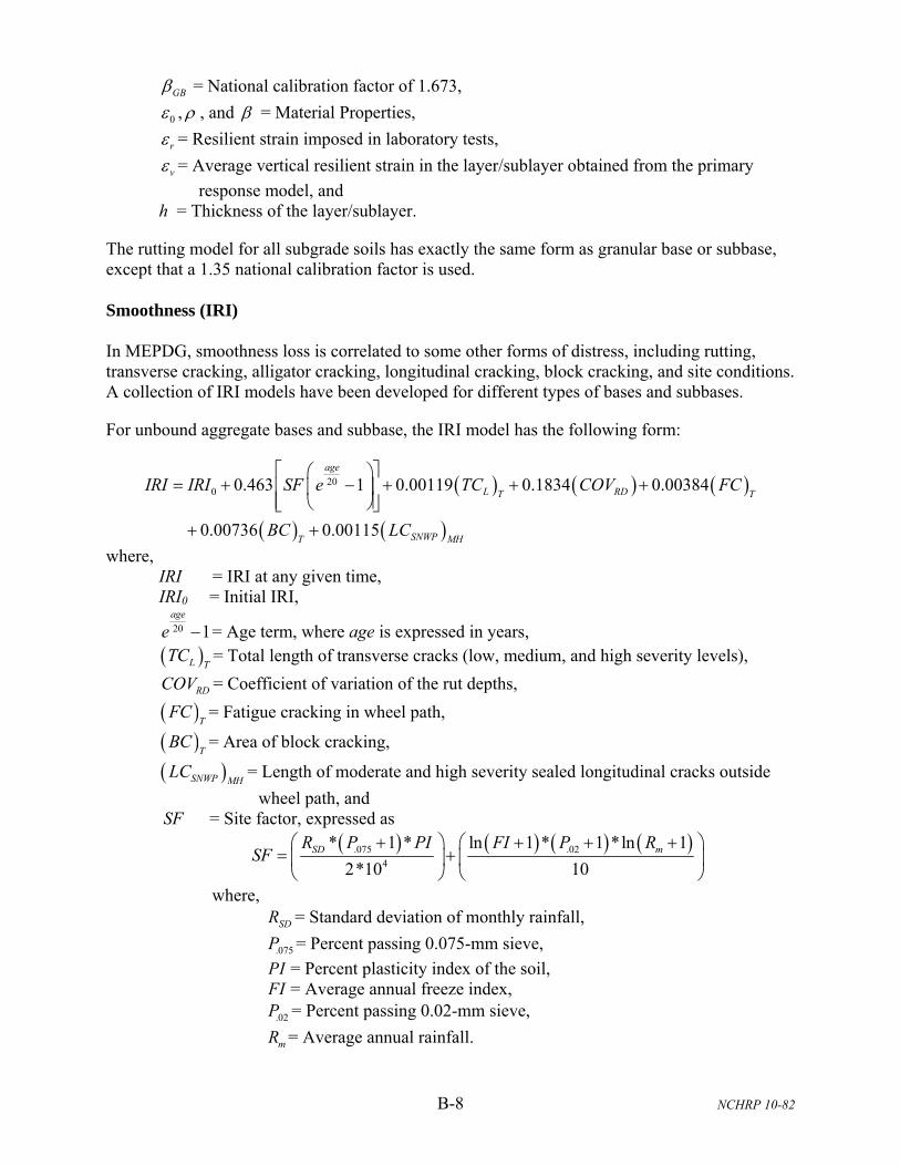
B-8 NCHRP 10-82

GB = National calibration factor of 1.673,

0 , , and = Material Properties,

r = Resilient strain imposed in laboratory tests,

v = Average vertical resilient strain in the layer/sublayer obtained from the primary

response model, and h = Thickness of the layer/sublayer.

The rutting model for all subgrade soils has exactly the same form as granular base or subbase, except that a 1.35 national calibration factor is used.

Smoothness (IRI)

In MEPDG, smoothness loss is correlated to some other forms of distress, including rutting, transverse cracking, alligator cracking, longitudinal cracking, block cracking, and site conditions. A collection of IRI models have been developed for different types of bases and subbases.

For unbound aggregate bases and subbase, the IRI model has the following form:

200 0.463 1 0.00119 0.1834 0.00384

0.00736 0.00115

age

L RDT T

SNWPT MH

IRI IRI SF e TC COV FC

BC LC

where, IRI = IRI at any given time, IRI0 = Initial IRI,

20 1age

e = Age term, where age is expressed in years,

L TTC = Total length of transverse cracks (low, medium, and high severity levels),

RDCOV = Coefficient of variation of the rut depths,

TFC = Fatigue cracking in wheel path,

TBC = Area of block cracking,

SNWP MHLC = Length of moderate and high severity sealed longitudinal cracks outside

wheel path, and SF = Site factor, expressed as

.075 .024

* 1 * ln 1 * 1 *ln 1

2*10 10SD mR P PI FI P R

SF

where,

SDR = Standard deviation of monthly rainfall,

.075P = Percent passing 0.075-mm sieve,

PI = Percent plasticity index of the soil, FI = Average annual freeze index,

.02P = Percent passing 0.02-mm sieve,

mR = Average annual rainfall.

B-9 NCHRP 10-82

For asphalt treated bases, the IRI model is as follows:

0 0.0099947 0.0005183 0.000235

118.36 0.9694

T

Hs H

IRI IRI Age FI FC

PTC

where,

s HTC = Average spacing of high severity transverse cracks,

HP = Area of high severity patches,

All other variables are as previously defined. For chemically treated bases, the IRI model is as follows:

0 0.00732 0.07647 0.0001449

0.00842 0.0002115

RD LT T

NWPT MH

IRI IRI FC SD TC

BC LC

where, all the variables are as previously defined. PERFORMANCE MODELS FOR PCC PAVEMENT

Concrete Pavement Faulting

The presence of water, the erodibility of a subbase material, the magnitude of load-inducted deflection, and the number of loads are factors that influence the development of faulting. However, existing models for faulting scarcely address these factors fully. Below are models listed in the literature that potentially could be used to predict faulting performance of PCC preservation treatments.

Markowl, 1984

An empirical model (see equation below) based on AASHO road test data related slab thickness to equivalent single axle load (ESAL) and subbase drainage conditions (Van Wijk 1985). The model is simple, but does not consider many important factors. The pumping index indicates the potential of erosion that increases with cumulative number of ESAL and diminishing drainage conditions but decreases quickly with an increase in slab thickness. Drainage adjustment factor is considered based on subbase permeability.

Dm

fESALmP di

34.007.1log

where, Pi = pumping index D = slab thickness (in.) ESAL = equivalent 80 kN (18,000 lb) single axle loads fd = drainage adjustment factor = 0.2 for good drainage (k =10,000 ft/day) = 0.6 for fair drainage (k = 100 ft/day) = 1.0 for poor drainage (k = 0.1 ft/day) k = subbase permeability

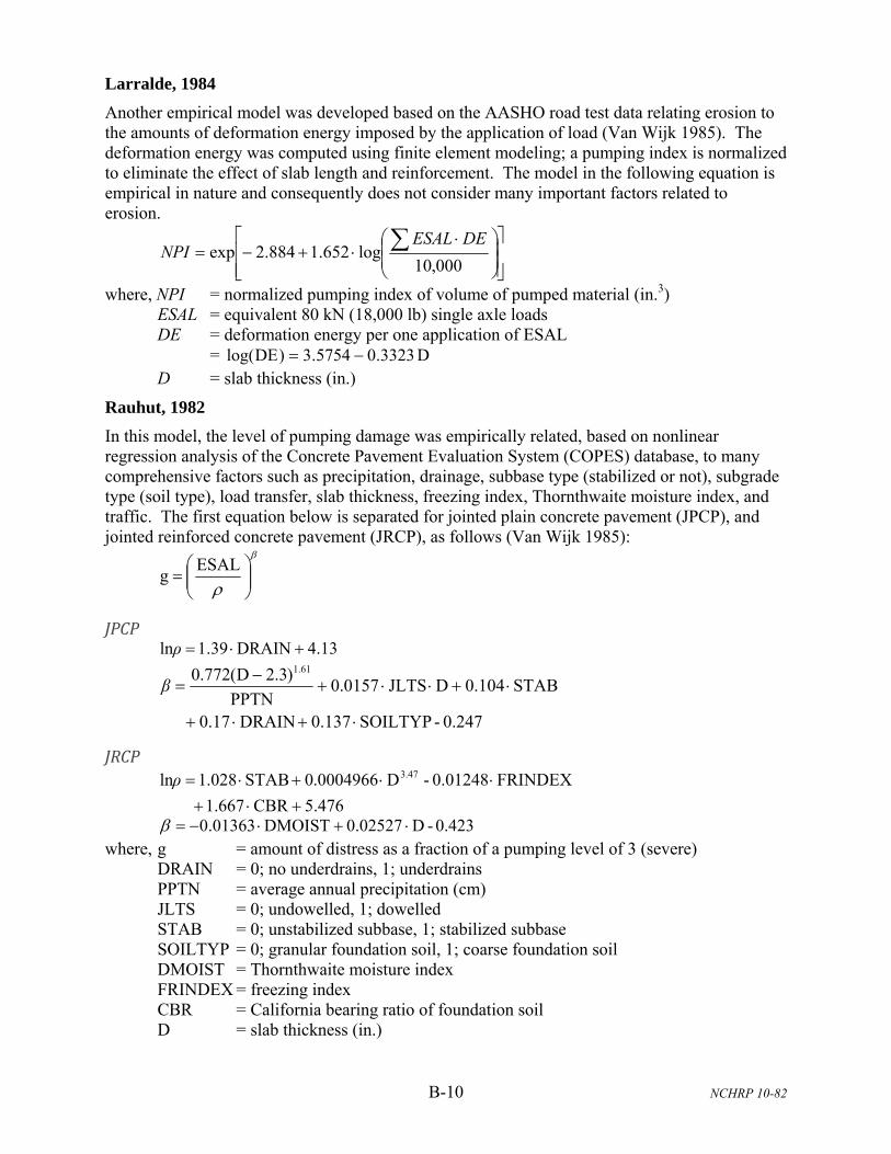
B-10 NCHRP 10-82

Larralde, 1984

Another empirical model was developed based on the AASHO road test data relating erosion to the amounts of deformation energy imposed by the application of load (Van Wijk 1985). The deformation energy was computed using finite element modeling; a pumping index is normalized to eliminate the effect of slab length and reinforcement. The model in the following equation is empirical in nature and consequently does not consider many important factors related to erosion.

000,10log652.1884.2exp

DEESALNPI

where, NPI = normalized pumping index of volume of pumped material (in.3) ESAL = equivalent 80 kN (18,000 lb) single axle loads DE = deformation energy per one application of ESAL = D3323.05754.3)DElog( D = slab thickness (in.)

Rauhut, 1982

In this model, the level of pumping damage was empirically related, based on nonlinear regression analysis of the Concrete Pavement Evaluation System (COPES) database, to many comprehensive factors such as precipitation, drainage, subbase type (stabilized or not), subgrade type (soil type), load transfer, slab thickness, freezing index, Thornthwaite moisture index, and traffic. The first equation below is separated for jointed plain concrete pavement (JPCP), and jointed reinforced concrete pavement (JRCP), as follows (Van Wijk 1985):

ESALg

JPCP 4.13DRAIN39.1ln ρ

0.247-SOILTYP0.137DRAIN0.17

STAB0.104DJLTS0157.0PPTN

)3.2D(772.0 61.1

β

JRCP

5.476CBR667.1

FRINDEX 0.01248-D0004966.0STAB028.1ln 3.47

ρ

0.423-D0.02527DMOIST01363.0 where, g = amount of distress as a fraction of a pumping level of 3 (severe) DRAIN = 0; no underdrains, 1; underdrains PPTN = average annual precipitation (cm) JLTS = 0; undowelled, 1; dowelled STAB = 0; unstabilized subbase, 1; stabilized subbase SOILTYP = 0; granular foundation soil, 1; coarse foundation soil DMOIST = Thornthwaite moisture index FRINDEX = freezing index CBR = California bearing ratio of foundation soil D = slab thickness (in.)

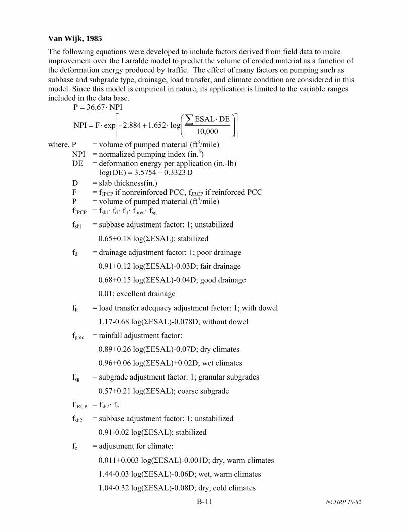
B-11 NCHRP 10-82

Van Wijk, 1985

The following equations were developed to include factors derived from field data to make improvement over the Larralde model to predict the volume of eroded material as a function of the deformation energy produced by traffic. The effect of many factors on pumping such as subbase and subgrade type, drainage, load transfer, and climate condition are considered in this model. Since this model is empirical in nature, its application is limited to the variable ranges included in the data base.

NPI36.67P

000,10

DEESALlog1.6522.884-expFNPI

where, P = volume of pumped material (ft3/mile) NPI = normalized pumping index (in.3) DE = deformation energy per application (in.-lb) D3323.05754.3)DElog( D = slab thickness(in.) F = fJPCP if nonreinforced PCC, fJRCP if reinforced PCC P = volume of pumped material (ft3/mile) fJPCP = fsbl· fd· flt· fprec· fsg

fsbl = subbase adjustment factor: 1; unstabilized

0.65+0.18 log(ΣESAL); stabilized

fd = drainage adjustment factor: 1; poor drainage

0.91+0.12 log(ΣESAL)-0.03D; fair drainage

0.68+0.15 log(ΣESAL)-0.04D; good drainage

0.01; excellent drainage

flt = load transfer adequacy adjustment factor: 1; with dowel

1.17-0.68 log(ΣESAL)-0.078D; without dowel

fprec = rainfall adjustment factor:

0.89+0.26 log(ΣESAL)-0.07D; dry climates

0.96+0.06 log(ΣESAL)+0.02D; wet climates

fsg = subgrade adjustment factor: 1; granular subgrades

0.57+0.21 log(ΣESAL); coarse subgrade

fJRCP = fsb2· fe

fsb2 = subbase adjustment factor: 1; unstabilized

0.91-0.02 log(ΣESAL); stabilized

fe = adjustment for climate:

0.011+0.003 log(ΣESAL)-0.001D; dry, warm climates

1.44-0.03 log(ΣESAL)-0.06D; wet, warm climates

1.04-0.32 log(ΣESAL)-0.08D; dry, cold climates

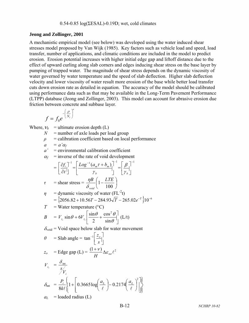
B-12 NCHRP 10-82

0.54-0.85 log(ΣESAL)-0.19D; wet, cold climates

Jeong and Zollinger, 2001

A mechanistic empirical model (see below) was developed using the water induced shear stresses model proposed by Van Wijk (1985). Key factors such as vehicle load and speed, load transfer, number of applications, and climatic conditions are included in the model to predict erosion. Erosion potential increases with higher initial edge gap and liftoff distance due to the effect of upward curling along slab corners and edges inducing shear stress on the base layer by pumping of trapped water. The magnitude of shear stress depends on the dynamic viscosity of water governed by water temperature and the speed of slab deflection. Higher slab deflection velocity and lower viscosity of water result more erosion of the base while better load transfer cuts down erosion rate as detailed in equation. The accuracy of the model should be calibrated using performance data such as that may be available in the Long-Term Pavement Performance (LTPP) database (Jeong and Zollinger, 2003). This model can account for abrasive erosion due friction between concrete and subbase layer.

0

a

iNf f e

Where, 0 = ultimate erosion depth (L) N = number of axle loads per load group ρ = calibration coefficient based on local performance a = a’f

a’ = environmental calibration coefficient f = inverse of the rate of void development

= 1

if

t

=

11 )(

b

mm baLog

=1

b

τ = shear stress =

1001

LTEB

void

η = dynamic viscosity of water (FL-2t) = 61002.26593.28456.1082.2056 TeTT

T = Water temperature (C)

B =

sin

cos

2

sin6sin

2

ii zz VV (L/t)

void = Void space below slab for water movement

θ = Slab angle =

s

zo1tan

zo = Edge gap (L) = 2)1( totH

izV =

iVs

int

int =

2

2174.0log3665.018

LLi aa

k

P

aL = loaded radius (L)

B-13 NCHRP 10-82

Pi = axle load (F) s = slab liftoff distance (L) = )1(2

γ = o

o

w

z

wo = k

Hρ

PCA Design Method

In this procedure, subbase erosion is related to pavement deflection (at the slab corner) due to axle loading. The following equations were developed based on the results of the AASHO Road Test for allowable load repetitions and erosion damage (Huang 2004):

103.01 )0.9(777.6524.14 log PCN

Percent erosion damage =

m

i i

i

N

nC

1

2100

where, N = allowable number of load repetitions based on a PSI of 3.0 C1 = adjustment factor (1 for untreated subbase, 0.9 for stabilized subbase)

P = rate of work or power = 73.0

2

7.268hk

p

p = pressure on the foundation under the slab corner in psi, p = kw k = modulus of subgrade reaction in psi/in w = corner deflection in inches h = thickness of slab in inches m = total number of load groups C2 = 0.06 for pavement without concrete shoulder, 0.94 for pavements with tied concrete

shoulder ni = predicted number of repetitions for ith load group Ni = allowable number of repetitions for ith load group Prepared sets of tables and charts are used to address doweled and aggregate interlock joints either with or without concrete shoulders. Since the erosion criterion was developed primarily from the results of the AASHTO Road Test using a specific subbase which was highly erodible, the application of the model has found limited use as far as application to different subbase types. Nonetheless, this procedure represents a significant advancement in the mechanistic analysis of pavement support condition in design.

AASHTO Design Method

Potential loss of support (LS) due to foundation erosion is utilized as input to effectively reduce the modulus of subgrade reaction in the thickness design procedure relative to four different contact conditions (i.e. with LS = 0, 1, 2, and 3). The best case is LS = 0, when the slab and foundation are assumed to be in full contact, while the worst case is LS = 3, when an area of slab is assumed not to be in contact with the subgrade (thus reduced values of k-value are in effect). In Table B-1, the possible ranges of LS factors for different types of subbase materials are provided to adjust the effective modulus of reaction. The subjectivity of the model reduces its sensitivity to material factors associated with erosion leading to inconsistency and limiting applicability. Load transfer coefficient and drainage coefficient are also indirectly related with

B-14 NCHRP 10-82

erosion; a lower deflection caused by better load transfer would reduce shear stress at the interface between the slab and base/subgrade as well as a shorter time of water presence due to better drainage may decrease the potential for pumping. Therefore, major factors causing erosion can be considered in the design.

Table B-1 Typical Ranges of LS Factors for Various Types of Materials (Huang 2004).

Type of material Loss of support Cement-treated granular base (E = 1x106 to 2x106 psi) 0.0 to 1.0 Cement aggregate mixtures (E = 500,000 to 1x106 psi) 0.0 to 1.0 Asphalt-treated bases(E = 350,000 to 1x106 psi) 0.0 to 1.0 Bituminous-stabilized mixture (E = 40,000 to 300,000 psi) 0.0 to 1.0 Lime-stabilized materials (E = 20,000 to 70,000 psi) 1.0 to 3.0 Unbound granular materials (E = 15,000 to 45,000 psi) 1.0 to 3.0 Fine-grained or natural subgrade materials (E = 3,000 to 40,000 psi) 2.0 to 3.0

Mechanistic-Empirical Pavement Design Guide (MEPDG)

The MEPDG addresses erosion in modeling faulting distress (see equations below) (ARA 2004). Classes of erodibility are formulated based on a modification of the Permanent International Association of Road Congresses (PIARC) specifications relative to material type and stabilizer percent. Five levels of erosion resistance are listed in Table B-2 distinguish between materials types based on stabilizer type and content (asphalt or portland cement) as well as long-term compressive strength (later than 28 days). Prediction of erodibility is closely associated with the stabilized material compressive strength and is readily available in most databases. Moreover, the presence of permeable drainage layer (treated or untreated granular material with permeability > 300 ft/day) and/or a geotextile fabric between the treated base and subgrade are design features to enhance design. Each class of erosion is assumed to offer 5 times the resistance to erosion than the next class. (i.e., class 1 materials are five times more erosion resistant than class 2 and so on). However, the guide do not address the degree of friction between the concrete and the base layer or its contribution to erosion of interface via shear stress. Field performance has been satisfactory even though lower strength materials have been used with low friction interface bases.

6)0.51( 51

70CEROD

m

jji CLogDECFAULTMAXFAULTMAX

6

)()0.51(5

2005120

C

ERODcurling P

WetDaysPLogCLogCFAULTMAX

where, FAULTMAXi = maximum mean transverse joint faulting for month i, in. FAULTMAX0 = initial maximum mean transverse joint faulting, in. EROD = base/subbase erodibility factor DEi = differential deformation energy accumulated during month i. EROD = base/subbase erodibility factor C12 = C1 + C2 * FR0.25

Ci = calibration constants FR = base freezing index defined as percentage of time the top base

temperature is below freezing (32 °F) temperature. δcurling = maximum mean monthly slab corner upward deflection PCC due to

temperature curling and moisture warping.

B-15 NCHRP 10-82

PS = overburden on subgrade, lb P200 = percent subgrade material passing #200 sieve WetDays = average annual number of wet days (greater than 0.1 in. rainfall).

Table B-2 MEPDG recommendations for assessing erosion potential of base material (ARA

2004).

Erodibility Class

Material Description and Testing

1

(a) Lean concrete with approximately 8 percent cement; or with long-term compressive strength > 2,500 psi (>2,000 psi at 28-days) and a granular subbase layer or a stabilized soil layer, or a geotextile fabric is placed between the treated base and subgrade, otherwise class 2. (b) Hot mixed asphalt concrete with 6 percent asphalt cement that passes appropriate stripping tests and aggregate tests and a granular subbase layer or a stabilized soil layer (otherwise class 2). (c) Permeable drainage layer (asphalt treated aggregate or cement treated aggregate and with an appropriate granular or geotextile separation layer placed between the treated permeable base and subgrade.

2

(a) Cement treated granular material with 5 percent cement manufactured in plant, or long-term compressive strength 2,000 to 2,500 psi (1,500 to 2,000 psi at 28-days) and a granular subbase layer or a stabilized soil layer, or a geotextile fabric is placed between the treated base and subgrade; otherwise class 3. (b) Asphalt treated granular material with 4 percent asphalt cement that passes appropriate stripping test and a granular subbase layer or a treated soil layer or a geotextile fabric is placed between the treated base and subgrade; otherwise class 3.

3

(a) Cement-treated granular material with 3.5 percent cement manufactured in plant, or with long-term compressive strength 1,000 to 2,000 psi (750 psi to 1,500 at 28-days). (b) Asphalt treated granular material with 3 percent asphalt cement that passes appropriate stripping test.

4 Unbound crushed granular material having dense gradation and high quality aggregates.

5 Untreated soils (PCC slab placed on prepared/compacted subgrade)

Pavement Macro-Surface Texture Model for Diamond Grinding

Data collected from studies of ground pavement surfaces indicate that the depth of texture is strongly dependant on the age or the time since the grinding and indirectly on traffic since grinding (Rao et al. 1999). Climate also seemed to be a factor as where pavements in wet and dry freeze environments tended to have lower macro texture than those in the non-freeze regions.

B-16 NCHRP 10-82

Pavement grinding on sections in the former regions would provide on the average 8 years of service life where those in the latter would provide 12 years of service life on the average. Several factors were considered in the development of the following macro-texture model listed as:

Time since grinding Traffic (both passenger and truck) since grinding Geographic location Annual temperature and moisture levels Freezing Index Blade spacing

The model for the mean texture depth (MTD) is: MTD = 0.152(1-0.233*Freeze)*Age + 0.887 where Age = Time since grinding (0.5 to 16 years) Freeze = Dummy variable for freeze climate region (0 = wet non-freeze or dry non-freeze, 1 = wet freeze or dry freeze region)

Prediction of Joint/Crack Spalling in PCC Pavement

Spalling is considered as one of the most important distress types of PCC pavement that affects the performance and functionality of a concrete pavement. Therefore it is useful to predict spalling in order to estimate future related maintenance i.e. partial depth repair or full depth repair and to examine how construction factors may affect pavement performance relative to spalling. Spalling is the breakdown or dislodging of concrete segments along or within 6 to 12 inches of a joint or crack in a concrete slab. There are two main steps associated with spalling. Step1: Initiation of delamination cracks: a significant contributor to spalling is the existence of shallow, horizontal delaminations that are oriented parallel to the alignment of a transverse crack or joint and at a shallow depth below the surface of the pavement. The formation of delamination has been researched for several years and has been found to be affected by a variety of factors but the most prevalent of them is the quality of the curing process and the evaporation of pore water from the concrete. If the moisture gradient due to evaporation is sufficiently severe it can create horizontal shear stresses and also cracks (Figure B-3.a). Step 2: The bending moment stress: the presence of delaminations in the vicinity of transverse cracking (in CRC pavement) can eventually lead to the development of spall damage due to repeated traffic loading or any number of mechanisms causing inplane bending stress in the delaminated segments (Figure B-3.b).

B-17 NCHRP 10-82

MEPDG Spall Model

Spalling is represented, however discretely, in the MEPDG design procedure. It has only been recently that any design procedure has attempted to address spall distress with a design methodology. The spalling model is used to determine a component of roughness along transverse joints used to determine the given level of IRI with the following model:

12*

100

0.01 1 1.005 Age SCF

AgeSPALL

Age

where SPALL = % Joints spalled (medium and high severities) Age = Pavement age, yrs SCF = Scaling factor based on site, design, and climate = -1400+350(%Air)(0.5 + Preform) + 3.4f’c(0.4) – 0.2(FTCYCAge) +

43hPCC – 536W/C %Air = Percent air in PCC

Preform = 1 if performed sealant; 0 if not f’c = PCC compressive strength, psi FYCYC = Average number of freeze-thaw cycles hPCC = Slab thickness, in W/C = water-cementitious ratio

Mechanistic Spall Stress and Performance Modeling

A spalling stress model by Tang et al. (1997) and Jeong, Zollinger (2001) serves as a means to determine tensile stress caused by passing wheel loads leading to spall development. The Tang model for spall stress (σ spall) is illustrated in Figure 2, which has since been modified from the original expression to account for tensile stress effects due to vertical shear on the crack face due to load transfer. As can be observed in Figure B-4, several key parameters are included in the model and are re-defined as follows:

Figure B-3 a) Initiation of delamination cracks, b) The bending moment stress.

Load

B-18 NCHRP 10-82

*

2

6

tanf

spall p f

M

t t

where,

τp = shear stress from tire loading τf = friction resistance at bottom of spall l* = length of spall θ = angle of spall fracture M = spall bending moment due to shear from load transfer The bracketed term in the equation can be used to calculate the stress that a passing wheel load causes on the surface concrete leading to chipping and shallow spalling. In case of spalling the second term principally applies.

Figure B-4. Concrete Pavement Spall Mechanism and Model. (Zollinger et al. 1994)

The bending stress, the main factor causing spall formation, can be easily calculated as a function of the load transfer of the transverse crack as imposed by ∆ which is deflection between loaded slab and unloaded slab. Since the bending moment is primarily affected by the aggregate interlock along the transverse crack, the spalling stress (σ spall) depends both on the induced bending moment and indirectly on slab thickness through its effect on the LTE of the transverse crack.

3

2*4

cE tM

where, l* = length of delamination (assumed to be 3 inches), ∆ = delamination opening at the face of the crack due to movement across the joint

or crack reflected in the load transfer efficiency, t = depth of spalling (in), and Ec = concrete modulus (psi)

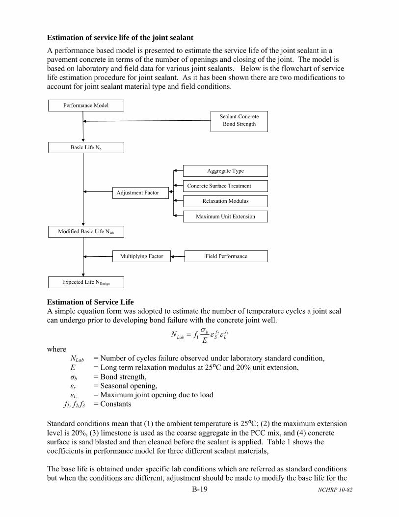
B-19 NCHRP 10-82

Estimation of service life of the joint sealant

A performance based model is presented to estimate the service life of the joint sealant in a pavement concrete in terms of the number of openings and closing of the joint. The model is based on laboratory and field data for various joint sealants. Below is the flowchart of service life estimation procedure for joint sealant. As it has been shown there are two modifications to account for joint sealant material type and field conditions.

Estimation of Service Life A simple equation form was adopted to estimate the number of temperature cycles a joint seal can undergo prior to developing bond failure with the concrete joint well.

321

ffbLab S LN f

E

where NLab = Number of cycles failure observed under laboratory standard condition, E = Long term relaxation modulus at 25⁰C and 20% unit extension, σb = Bond strength, εs = Seasonal opening, εL = Maximum joint opening due to load

f1, f2,f3 = Constants Standard conditions mean that (1) the ambient temperature is 25⁰C; (2) the maximum extension level is 20%, (3) limestone is used as the coarse aggregate in the PCC mix, and (4) concrete surface is sand blasted and then cleaned before the sealant is applied. Table 1 shows the coefficients in performance model for three different sealant materials, The base life is obtained under specific lab conditions which are referred as standard conditions but when the conditions are different, adjustment should be made to modify the base life for the

Performance Model

Sealant-Concrete Bond Strength

Basic Life Nb

Aggregate Type

Relaxation Modulus

Maximum Unit Extension

Concrete Surface Treatment Adjustment Factor

Modified Basic Life Nlab

Field Performance Multiplying Factor

Expected Life NDesign

B-20 NCHRP 10-82

standard conditions to the modified base life. Main factors that affect the service life of the joint sealants include aggregate type, surface preparation, relaxation modulus of the sealant and strains due to seasonal changes and load. The adjustment is made through the following equation:

mod

1 2 3 4

m lab

m

N a N

a a a a a

where Nmod = Modified base life in number of cycles to failure Nlab = Base life under standard conditions and am = Overall adjustment factor (component factors listed in Tables B-3 through B-6)

a1 is adjustment for aggregate,a2 is adjustment for preparation technique and a3 is adjustment factor for long term relaxation modulus and a4 is the adjustment factor for the expected maximum unit extension level. In order to formulate a reasonable estimate the service life of a joint seal it is important to ascertain the effect of different variables such as geographical location of site, traffic volume, etc on performance. This is done by assuming that the field performance trends well with a weibull distribution and that such a curve can be constructed to fit the observed data points thus characterizing the performance of the sealant at particular field site over time. This effort will require that field data be collected and analyzed for the determination of the two Weibull distribution parameters called the shape (γ) and scale factors (λ). Using the Weibull relationship, load cycles can be related to the damage level (as measured in terms of full depth debonding failure) as:

11

lnf bN d

where Nf = number of load cycles γ = shape factor λ = scale factor db = percentage of the sealant in the joint length where full depth debonding

has occurred. Table B-3 Adjustment factor for aggregate type.

Aggregate Type Adjustment factor a1

Sealant Type 1 Sealant Type 2 Sealant Type 3

Limestone 1 1 1

River Gravel 1.15 1.16 1.19

B-21 NCHRP 10-82

Table B-4 Adjustment factor for preparation technique.

Surface Preparation Adjustment factor a2

Sealant Type 1 Sealant Type 2 Sealant Type 3

Sand Blast 1 1 1

Water Blast+ Sand Blast 1 0.973 0.917

Sand Blast + Primer 1 1 1.26

Table B-5 Adjustment factor for relaxation modulus.

Unit Extension Level Adjustment factor a3

Class 1 Class 2 Class 3

Above the Standard 0.9 0.9 0.9

Equal 1 1 1

Below the Standard 1.1 1.1 1.1

Table B-6 Adjustment factor for unit extension level.

Unit Extension Level Adjustment factor a4

Class 1 Class 2 Class 3

10% 1.91 1.33 1.75

20% 1 1 1

30% 0.75 0.9 0.63

40% 0.51 0.75 0.47

The relationship between Nf and db can be determined for each pavement and sealant type. Based on tests data from Phoenix, Arizona γ=0.522 and lnλ =19.39 for silicon based sealants and γ=.83 and lnλ =17.78 for asphalt base sealants for dry, on freeze areas. These values can be used where the climate is similar to Arizona. For a chosen maximum value of db referred to as dbmax corresponding life Nfc can be determined easily as:

1

max

1ln

cf bN d

where Nfc is the number of cycles to failure corresponding to db max For a given design unit extension level, d, the life can be determined using the following equation:

mod

df design

c

NN

MF

where f designN = Expected design life at the field conditions

B-22 NCHRP 10-82

f lab dN = Expected life at the extension level of d in the libratory

MFc = Multiplying factor,

mod

maxc

f

cf b

NMF

N d

εf = Sealant strain level in the field section d b max = Maximum allowable debonding

Delamination Modeling

Shear stress (or delamination stress) can be determined based on slab curling and warping behavior under the effect of drying shrinkage and temperature change. Slab warping (mainly driven by differential drying shrinkage) can occur in two stages as denoted by Zollinger et al. (1994) and delineated by separation of the slab corner from the subbase (i.e. liftoff) versus where the slab remains in contact with the subbase (i.e. zero liftoff). Medium-thick plate theory provides the basis for several boundary conditions that were considered in the development of the coefficient equations summarized in Table 3. Two sets of solutions of the coefficient equations were developed depending whether the bottom of the slab was in contact with the subgrade or base support. References Applied Research Associates (ARA). (2004). Guide for Mechanistic-Empirical Design of New and Rehabilitated Pavement Structures (Final Report), National Cooperative Highway Research Program, http://www.trb.org/mepdg/guide.htm, accessed: December 1, 2010.

Eltahan A. A., Daleiden J. F., and Simpson A. L. (1999). Effectiveness of Maintenance Treatments of Flexible Pavements, Transportation Research Record: Journal of the Transportaiton Research Board, No. 1680, TRB, National Research Council, Washington D.C., pp. 18-25.

Hajek, J.J, and Bradbury, A. (1996). Pavement Performance Modeling using Canadian Strategic Highway Research Program Bayesian Statistical Methodology, Transportation Research Record: Journal of the Transportation Research Board, No. 1524, Transportation Research Record No. 1524, pp. 160.

Huang, Y.H. (2004), “Pavement Analysis and Design, 2nd Edition,” Pearson Prentice Hall, Upper Saddle River, New Jersey.

Jahren C. T., Cawley B., Ellsworth B., and Bergeson K. (1999). Cold In-Place Asphalt Recycling Performance Review, in the proceedings of the Fifth ASCE Materials Engineering Congress, Cincinnati, Ohio, pp. 794-801.

Jeong J. and D. Zollinger, “Characterization of Stiffness Parameters in Design of Continuously Reinforced and Jointed Pavements,” Transportation Research Record 1778, TRB, National Research Council, Washington, D.C., 2001, pp. 54-63.

Labi S., Lamptey G., and Kong S. (2007a). Effective of Microsurfacing Treatments, Journal of Transportation Engineering, Vol. 133, Issue 5, pp. 298-307.

B-23 NCHRP 10-82

Labi S., Mahmodi M.I., Fang C., and Nunoo C. (2007b). Cost-Effectiveness of Microsurfacing and Thin HMA Overlays - A Comparative Analysis, in the cd-rom of the 86th Transportation Research Board Annual Meeting.

Liu L., Hossain M., and Miller R. (2009). Modeling of Chip Seal Performance on Kansas Highways, in the Proceedings of Mid-Continent Transportation Research Symposium, Ames, Iowa.

Morian D. A., Gibson S. D., and Epps J. A. (1998). Maintaining Flexible Pavements - The Long Term Pavement Performance Experiment SPS-3 5-Year Data Analysis, FHWA-RD-97-102 Report, U.S. Department of Transportation.

Morian D. A., Oswalt J., Deodhar A. (2004). Experience with Cold In-Place Recycling as a Reflective Crack Control Technique, Transportation Research Record: Journal of the Transportation Research Board, No. 1869, TRB, National Research Council, Washington D.C., pp. 47-55.

Rao, Shreenath, H. Thomas Yu, and Michael I. Darter, “The Longevity and Performance of Diamond-Ground Pavements,” R&D Bulletin RD 118, Portland Cement Association, 1999.

Sebaaly P. E., Bazi G., Hitti E., Weitzel D., and Bemanian S. (2004). Performance of Cold In-Place Recycling in Nevada, Transportation Research Record: Journal of the Transportation Research Board, No. 1896, TRB, National Research Council, Washington D.C., 2004, pp. 162-169.

Tang, T. and D.G. Zollinger. (1997). Investigation of Spall Repair for Concrete Pavements. Research Report TX-98/2919-3, TTI 2919-3, Texas Transportation Institute, The Texas A&M University System, Texas Department of Transportation.

Temple W., Shah S., Paul H., and Abadie C. (2002). Performance of Louisiana's Chip Seal and Microsurfacing Program, 2002, Transportation Research Record: Journal of the Transportation Research Board, No. 1795, TRB, National Research Council, Washington D.C., pp. 3-16.

Van Wijk, A. J., “Rigid Pavement Pumping: (1) Subbase Erosion and (2) Economic Modeling,” Joint Highway Research Project File 5-10. School of Civil Engineering, Purdue University, West Lafayette, Ind., May 16, 1985.

Zollinger, Dan G., Sanjaya P. Senadheera, and Tianxi Tang, "Spalling of Continuously Reinforced Concrete Pavements," Vol. 120 No.3, ASCE Journal of Transportation Engineering, May/June 1994, pp.394-411.

C-1 NCHRP 10-82

Appendix C. Promising HMA Treatment Sections from the LTPP Database.

Chip Seal

Section ID

State County Route

No. Freezing

Index Annual Prec., in

AADTT, Trucks/day

Const. Date

Seal Thick,

in

HMA Thick*,

in

Base Thick,

in Base Type

Subgrade Type

A350 Utah GARFIELD 89 302 9.47 131 7/18/1990 0.2 7.1 9.5 A-1-a Silty Sand B350 Utah SEVIER 89 242 9.39 158 7/18/1990 0.3 5.5 5.5 A-1-a Silty Sand C350 Arizona PIMA 19 0 14.58 1082 9/6/1990 0.3 8 6 A-1-a Clayey Sand

M350 Texas DUVAL 59 1 26.46 310 10/18/1990 0.2 1.5 8 A-2-4 Clay (Liquid Limit > 50)

B350 Oklahoma SEMINOLE 3E 77 37.91 273 9/10/1990 0.3 10.3 N/A N/A Sand A350 Washington SPOKANE 195 281 16.79 288 8/12/1990 0.2 3.6 11.4 A-1-a Gravel

A350 Oklahoma JACKSON 62 57 27.88 381 9/12/1990 0.3 10 6 Cement-Treated Subgrade Soil

Clay (Liquid Limit > 50)

A350 Arizona MOHAVE 93 0 5.97 957 9/11/1990 0.2 3.5 16 A-1-a Sandy Clay

A350 California BUTTE 32 0 35.00 143 8/21/1990 0.3 4.8 15 A-1-a

Poorly Graded Gravel

L350 Texas EL PASO 62 5 9.70 275 9/20/1990 0.2 1.5 8.5 A-2-4 Sand

H350 Texas GRIMES 105 6 43.81 233 10/11/1990 0.2 1 8 A-1-a Clay (Liquid Limit > 50)

B350 Arizona MOHAVE 40 2 8.84 1423 8/27/1990 0.3 6 9 A-1-b Clayey Sand

Q350 Texas MILLS 84 17 29.15 216 9/25/1990 0.3 1.5 12 Crushed Stone, Gravel or Slag

Clayey Gravel

J350 Texas WILSON 181 2 29.91 205 10/16/1990 0.2 3 6 A-1-a Sandy Clay

I350 Texas WALKER 30 8 47.59 207 10/10/1990 0.1 8 12 Other Clay (Liquid Limit > 50)

C350 Oklahoma KAY 60 134 34.69 243 9/7/1990 0.3 12.5 6 A-6 Silty Clay G350 Texas RUSK 322 18 48.68 222 10/5/1990 0.2 1.5 12 A-2-4 Sand F350 Texas VAN ZANDT 19 29 43.26 317 10/4/1990 0.3 1.5 6 A-1-a Sandy Clay

B350 Idaho JEFFERSON 20 598 12.89 539 8/5/1990 0.2 4.8 4.8 A-1-a Clayey Gravel

N350 Texas KENEDY 77 0 27.61 654 10/19/1990 0.4 2.5 8 A-2-4 Sand A350 Idaho JEROME 93 282 10.57 189 7/30/1990 0.2 4.2 12 A-1-a Silt A350 Montana JUDITH BASIN 87 662 16.94 173 8/10/1990 0.2 3 10.5 A-1-a Silty Clay C350 Florida VOLUSIA 442 0 53.23 223 8/17/1990 0.3 1.3 8.7 A-1-b Sand B350 Washington DOUGLAS 2 269 9.87 46 8/13/1990 0.5 1.8 3.6 A-1-a Gravel A350 Alabama MONTGOMERY 152 7 54.07 745 8/7/1990 0.3 10.5 6 Soil-Aggregate Mixture Sandy Clay A350 Mississippi COVINGTON 84 10 57.61 260 8/23/1990 0.3 8.5 4.5 A-2-4 Silty Sand B350 Nevada ELKO 80 312 6.94 627 7/29/1990 0.2 9.8 4 A-1-a Gravel

C-2 NCHRP 10-82

Section ID

State County Route

No. Freezing

Index Annual Prec., in

AADTT, Trucks/day

Const. Date

Seal Thick,

in

HMA Thick*,

in

Base Thick,

in Base Type

Subgrade Type

E350 Texas GARZA 84 55 20.62 447 9/14/1990 0.3 6.5 7.5 A-2-6 Clayey Sand

B350 Texas KAUFMAN 175 22 38.81 549 9/26/1990 0.3 9.5 10 A-2-5 Clay (Liquid Limit > 50)

B350 Florida CLAY 17 0 50.51 711 8/16/1990 0.4 3 12 Sand Sand A350 Nevada WASHOE 650 105 7.80 120 8/22/1990 0.3 7.8 12 A-1-a Clayey Silt

A350 Arkansas BENTON 71 128 44.46 1244 9/5/1990 0.2 16.5 N/A N/A Clay (Liquid Limit > 50)

K350 Texas BEXAR 1560 4 33.31 148 10/15/1990 0.3 1 9 A-2-6 Clay (Liquid Limit > 50)

C350 Alabama HOUSTON 84 7 56.43 438 8/9/1990 0.3 3.7 6 A-1-a Clayey Sand C350 Nevada ELKO 80 368 9.27 581 7/28/1990 0.4 8.8 54 A-1-a Sandy Silt D350 Arizona SANTA CRUZ 19 0 15.37 1288 9/6/1990 0.2 11 7 A-1-a Gravel A350 Florida NASSAU 200 1 50.89 391 8/13/1990 0.3 4 12 Soil-Aggregate Mixture Sand

B350 Tennessee DE KALB 56 108 56.34 97 8/2/1990 0.3 5.6 8 Crushed Stone, Gravel or Slag Rock

C350 Tennessee ANDERSON 75 89 55.13 3282 8/3/1990 0.3 11.3 10 Crushed Stone, Gravel or Slag Silty Clay

D350 Texas MITCHELL 20 32 20.78 1126 9/18/1990 0.1 11 6 A-2-6 Sandy Clay

A350 Missouri MILLER 54 200 40.28 499 8/19/1990 0.3 9 4 Crushed Stone, Gravel or Slag Sandy Clay

A350 Minnesota BELTRAMI 71 1466 25.85 117 7/28/1990 0.2 3 4 A-3 Sand D350 Minnesota MILLE LACS 169 1065 30.19 152 7/31/1990 0.3 4.8 6 A-1-b Sand B350 Minnesota BELTRAMI 2 1465 25.89 351 7/28/1990 0.1 6.8 12 Gravel (Uncrushed) Sand C350 Minnesota OTTER TAIL 10 1296 26.57 275 7/30/1990 0.2 9.5 N/A N/A Sand A350 Nebraska FURNAS 6 360 23.18 140 7/17/1990 0.2 7 N/A N/A Silt A350 Kansas FRANKLIN 68 249 37.17 145 7/12/1990 0.2 11.5 N/A N/A Silty Clay B350 Alabama WASHINGTON 43 4 64.38 280 8/21/1990 0.3 7 5 A-1-b Silty Sand B350 Michigan MECOSTA 131 600 35.02 288 8/8/1990 0.3 6 18 A-1-a Sandy Clay

* The HMA thickness refers to the total thickness of all the HMA layers (i.e., the original HMA surface and HMA overlay(s) applied later).

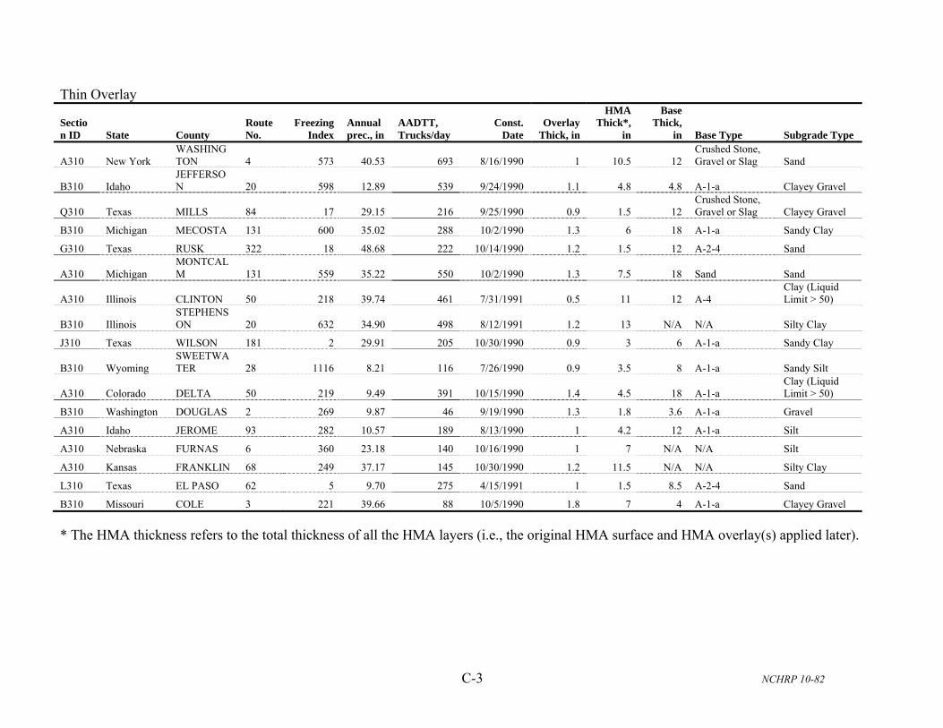
C-3 NCHRP 10-82

Thin Overlay

Section ID State County

Route No.

Freezing Index

Annual prec., in

AADTT, Trucks/day

Const. Date

Overlay Thick, in

HMA Thick*,

in

Base Thick,

in Base Type Subgrade Type

A310 New York WASHINGTON 4 573 40.53 693 8/16/1990 1 10.5 12

Crushed Stone, Gravel or Slag Sand


Q310 Texas MILLS 84 17 29.15 216 9/25/1990 0.9 1.5 12 Crushed Stone, Gravel or Slag Clayey Gravel

B310 Michigan MECOSTA 131 600 35.02 288 10/2/1990 1.3 6 18 A-1-a Sandy Clay

G310 Texas RUSK 322 18 48.68 222 10/14/1990 1.2 1.5 12 A-2-4 Sand

A310 Michigan MONTCALM 131 559 35.22 550 10/2/1990 1.3 7.5 18 Sand Sand

A310 Illinois CLINTON 50 218 39.74 461 7/31/1991 0.5 11 12 A-4 Clay (Liquid Limit > 50)

B310 Illinois STEPHENSON 20 632 34.90 498 8/12/1991 1.2 13 N/A N/A Silty Clay


B310 Wyoming SWEETWATER 28 1116 8.21 116 7/26/1990 0.9 3.5 8 A-1-a Sandy Silt

A310 Colorado DELTA 50 219 9.49 391 10/15/1990 1.4 4.5 18 A-1-a Clay (Liquid Limit > 50)

B310 Washington DOUGLAS 2 269 9.87 46 9/19/1990 1.3 1.8 3.6 A-1-a Gravel

A310 Idaho JEROME 93 282 10.57 189 8/13/1990 1 4.2 12 A-1-a Silt

A310 Nebraska FURNAS 6 360 23.18 140 10/16/1990 1 7 N/A N/A Silt

A310 Kansas FRANKLIN 68 249 37.17 145 10/30/1990 1.2 11.5 N/A N/A Silty Clay

L310 Texas EL PASO 62 5 9.70 275 4/15/1991 1 1.5 8.5 A-2-4 Sand

B310 Missouri COLE 3 221 39.66 88 10/5/1990 1.8 7 4 A-1-a Clayey Gravel


C-4 NCHRP 10-82

Slurry Seal

Sec. ID State County

Route No.

Freezing Index

Annual prec., in

AADTT, Trucks/day

Const. Date

Seal Thick,

in

HMA Thick*,

in

Base Thick,


B320 Missouri COLE 3 221 39.66 88 8/18/1990 0.1 7 4 A-1-a Clayey Gravel

M320 Texas DUVAL 59 1 26.46 310 10/18/1990 0.1 1.5 8 A-2-4 Clay (Liquid Limit > 50)

A320 Nebraska FURNAS 6 360 23.18 140 7/17/1990 0.1 7 N/A N/A Silt

A320 Utah GARFIELD 89 302 9.47 131 7/2/1990 0.2 7.1 9.5 A-1-a Silty Sand

A320 Michigan MONTCALM 131 559 35.22 550 8/7/1990 0.1 7.5 18 Sand Sand

H320 Texas GRIMES 105 6 43.81 233 10/11/1990 0.2 1 8 A-1-a Clay (Liquid Limit > 50)

D320 Arizona SANTA CRUZ 19 0 15.37 1288 9/6/1990 0.1 11 7 A-1-a Gravel

B320 Washington DOUGLAS 2 269 9.87 46 8/13/1990 0.2 1.8 3.6 A-1-a Gravel

B320 Wyoming SWEETWATER 28 1116 8.21 116 7/26/1990 0.2 3.5 8 A-1-a Sandy Silt

B320 Nevada ELKO 80 312 6.94 627 7/29/1990 0.1 9.8 4 A-1-a Gravel

C320 Alabama HOUSTON 84 7 56.43 438 8/9/1990 0.2 3.7 6 A-1-a Clayey Sand

C320 Florida VOLUSIA 442 0 53.23 223 8/18/1990 0.2 1.3 8.7 A-1-b Sand

A320 Washington SPOKANE 195 281 16.79 288 8/12/1990 0.2 3.6 11.4 A-1-a Gravel

A320 Tennessee CANNON 96 88 55.97 71 7/30/1990 0.3 8.6 5 Crushed Stone, Gravel or Slag Silty Clay

I320 Texas WALKER 30 8 47.59 207 10/10/1990 0.2 8 12 Other Clay (Liquid Limit > 50)

A320 Mississippi COVINGTON 84 10 57.61 260 8/23/1990 0.3 8.5 4.5 A-2-4 Silty Sand

A320 Nevada WASHOE 650 105 7.80 120 8/22/1990 0.3 7.8 12 A-1-a Clayey Silt

C320 Washington CLARK 14 23 62.28 128 8/15/1990 0.2 8.4 3.6 A-1-a Gravel

B320 Texas KAUFMAN 175 22 38.81 549 9/26/1990 0.2 9.5 10 A-2-5 Clay (Liquid Limit > 50)

B320 Florida CLAY 17 0 50.51 711 8/16/1990 0.3 3 12 Sand Sand

D320 Minnesota MILLE LACS 169 1065 30.19 152 7/31/1990 0.3 4.8 6 A-1-b Sand

C320 Minnesota OTTER TAIL 10 1296 26.57 275 7/30/1990 0.1 9.5 N/A N/A Sand

E320 Texas GARZA 84 55 20.62 447 9/14/1990 0.2 6.5 7.5 A-2-6 Clayey Sand

C320 Oklahoma KAY 60 134 34.69 243 9/7/1990 0.2 12.5 6 A-6 Silty Clay

C-5 NCHRP 10-82


Route No.

Freezing Index

Annual prec., in

AADTT, Trucks/day

Const. Date

Seal Thick,

in

HMA Thick*,

in

Base Thick,


A320 Florida NASSAU 200 1 50.89 391 8/13/1990 0.2 4 12 Soil-Aggregate Mixture Sand

A320 California BUTTE 32 0 35.00 143 8/21/1990 0.3 4.8 15 A-1-a Poorly Graded Gravel

A320 Alabama MONTGOMERY 152 7 54.07 745 8/7/1990 0.2 10.5 6

Soil-Aggregate Mixture Sandy Clay


A320 Arkansas BENTON 71 128 44.46 1244 9/5/1990 0.2 16.5 N/A N/A Clay (Liquid Limit > 50)

B320 Arizona MOHAVE 40 2 8.84 1423 8/27/1990 0.2 6 9 A-1-b Clayey Sand

B320 Alabama WASHINGTON 43 4 64.38 280 8/21/1990 0.2 7 5 A-1-b Silty Sand

F320 Texas VAN ZANDT 19 29 43.26 317 10/4/1990 0.1 1.5 6 A-1-a Sandy Clay

C320 Arizona PIMA 19 0 14.58 1082 9/5/1990 0.1 8 6 A-1-a Clayey Sand

A320 Missouri MILLER 54 200 40.28 499 8/19/1990 0.1 9 4 Crushed Stone, Gravel or Slag Sandy Clay


A320 Idaho JEROME 93 282 10.57 189 7/30/1990 0.2 4.2 12 A-1-a Silt

A320 Arizona MOHAVE 93 0 5.97 957 8/24/1990 0.1 3.5 16 A-1-a Sandy Clay

A320 Colorado DELTA 50 219 9.49 391 8/31/1990 0.2 4.5 18 A-1-a Clay (Liquid Limit > 50)

A320 Indiana SPENCER 64 185 48.04 1078 8/16/1990 0.2 15.8 N/A N/A Silty Clay

B320 Kentucky BARREN PRKWY 118 53.43 230 8/15/1990 0.2 15 N/A N/A


A320 Iowa SAC 196 711 30.93 77 8/23/1990 0.2 9 6 Gravel (Uncrushed) Sandy Clay

C320 Nevada ELKO 80 368 9.27 581 7/28/1990 0.4 8.8 54 A-1-a Sandy Silt

A320 Montana JUDITH BASIN 87 662 16.94 173 8/7/1990 0.2 3 10.5 A-1-a Silty Clay

B320 Utah SEVIER 89 242 9.39 158 7/5/1990 0.1 5.5 5.5 A-1-a Silty Sand

K320 Texas BEXAR 1560 4 33.31 148 10/15/1990 0.2 1 9 A-2-6 Clay (Liquid Limit > 50)

A320 Oklahoma JACKSON 62 57 27.88 381 9/12/1990 0.2 10 6 Cement-Treated Subgrade Soil


D320 Texas MITCHELL 20 32 20.78 1126 9/18/1990 0.1 11 6 A-2-6 Sandy Clay

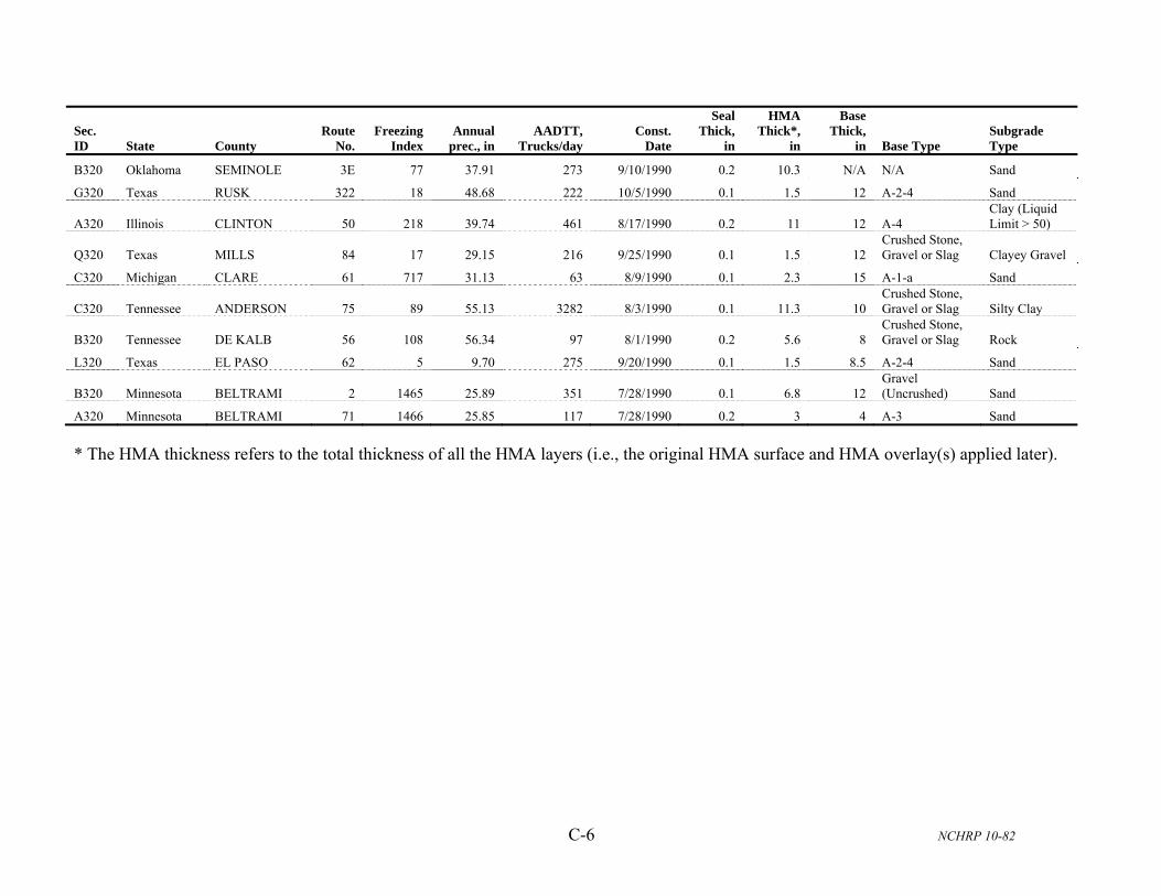
C-6 NCHRP 10-82


Route No.

Freezing Index

Annual prec., in

AADTT, Trucks/day

Const. Date

Seal Thick,

in

HMA Thick*,

in

Base Thick,


B320 Oklahoma SEMINOLE 3E 77 37.91 273 9/10/1990 0.2 10.3 N/A N/A Sand

G320 Texas RUSK 322 18 48.68 222 10/5/1990 0.1 1.5 12 A-2-4 Sand

A320 Illinois CLINTON 50 218 39.74 461 8/17/1990 0.2 11 12 A-4 Clay (Liquid Limit > 50)

Q320 Texas MILLS 84 17 29.15 216 9/25/1990 0.1 1.5 12 Crushed Stone, Gravel or Slag Clayey Gravel

C320 Michigan CLARE 61 717 31.13 63 8/9/1990 0.1 2.3 15 A-1-a Sand

C320 Tennessee ANDERSON 75 89 55.13 3282 8/3/1990 0.1 11.3 10 Crushed Stone, Gravel or Slag Silty Clay

B320 Tennessee DE KALB 56 108 56.34 97 8/1/1990 0.2 5.6 8 Crushed Stone, Gravel or Slag Rock

L320 Texas EL PASO 62 5 9.70 275 9/20/1990 0.1 1.5 8.5 A-2-4 Sand

B320 Minnesota BELTRAMI 2 1465 25.89 351 7/28/1990 0.1 6.8 12 Gravel (Uncrushed) Sand

A320 Minnesota BELTRAMI 71 1466 25.85 117 7/28/1990 0.2 3 4 A-3 Sand


C-7 NCHRP 10-82

Crack Sealing

Sec. ID State County Route

No.Freezing

IndexAnnual

prec., inAADTT,

Trucks/dayConst.

Date HMA

Thick*, inBase

Thick, inBase Type Subgrae Type

A330 Alabama MONTGOMERY 152 7 54.07 745 8/7/1990 10.5 6 Soil-Aggregate Mixture (Predominantly Fine-Grained Soil)

Sandy Clay

A330 Arizona MOHAVE 93 0 5.97 957 8/24/1990 3.5 16 A-1-a Sandy Clay

A330 California BUTTE 32 0 35.00 143 8/21/1990 4.8 15 A-1-a Poorly Graded Gravel

B330 Colorado BENT 50 219 13.10 260 7/24/1990 11.5 N/A N/A Clay (Liquid Limit > 50)

C330 Florida VOLUSIA 442 0 53.23 223 8/17/1990 1.3 8.7 A-1-b Sand

A330 Illinois CLINTON 50 218 39.74 461 8/17/1990 11 12 A-4 Clay (Liquid Limit > 50)

B330 Illinois STEPHENSON 20 632 34.90 498 8/2/1990 13 N/A N/A Silty Clay

A330 Indiana SPENCER 64 185 48.04 1078 8/16/1990 15.8 N/A N/A Silty Clay

A330 Iowa SAC 196 711 30.93 77 7/10/1990 9 6 Gravel (Uncrushed) Sandy Clay

B330 Kansas FORD 400 204 23.18 336 7/14/1990 8 39 Clayey Sand Sandy Clay

B330 Minnesota BELTRAMI 2 1465 25.89 351 7/28/1990 6.8 12 Gravel (Uncrushed) Sand

A330 Missouri MILLER 54 200 40.28 499 8/19/1990 9 4 Crushed Stone, Gravel or Slag

Sandy Clay

B330 Missouri COLE 3 221 39.66 88 8/18/1990 7 4 A-1-a Clayey Gravel

A330 Nebraska FURNAS 6 360 23.18 140 7/17/1990 7 N/A N/A Silt

A330 Nevada WASHOE 650 105 7.80 120 8/22/1990 7.8 12 A-1-a Clayey Silt

B330 Nevada ELKO 80 312 6.94 627 7/29/1990 9.8 4 A-1-a Gravel

B330 Oklahoma SEMINOLE 3E 77 37.91 273 9/10/1990 10.3 N/A N/A Sand

B330 Pennsylvania TIOGA 49 467 37.28 76 10/2/1990 6.5 17 Gravel (Uncrushed) Silty Clay

A330 Tennessee CANNON 96 88 55.97 71 7/30/1990 8.6 5 Crushed Stone, Gravel or Slag

Silty Clay

C330 Tennessee ANDERSON 75 89 55.13 3282 8/3/1990 11.3 10 Crushed Stone, Gravel or Slag

Silty Clay

D330 Texas MITCHELL 20 32 20.78 1126 9/18/1990 11 6 A-2-6 Sandy Clay

L330 Texas EL PASO 62 5 9.70 275 9/20/1990 1.5 8.5 A-2-4 Sand

A330 Utah GARFIELD 89 302 9.47 131 7/2/1990 7.1 9.5 A-1-a Silty Sand

B330 Utah SEVIER 89 242 9.39 158 7/5/1990 5.5 5.5 A-1-a Silty Sand

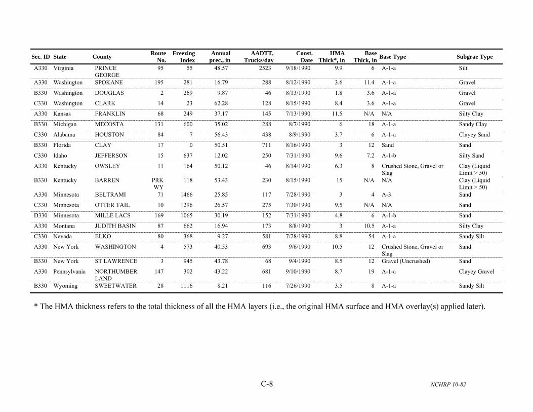
C-8 NCHRP 10-82

Sec. ID State County Route

No.Freezing

IndexAnnual

prec., inAADTT,

Trucks/dayConst.

Date HMA

Thick*, inBase

Thick, inBase Type Subgrae Type

A330 Virginia PRINCE GEORGE

95 55 48.57 2523 9/18/1990 9.9 6 A-1-a Silt

A330 Washington SPOKANE 195 281 16.79 288 8/12/1990 3.6 11.4 A-1-a Gravel

B330 Washington DOUGLAS 2 269 9.87 46 8/13/1990 1.8 3.6 A-1-a Gravel

C330 Washington CLARK 14 23 62.28 128 8/15/1990 8.4 3.6 A-1-a Gravel

A330 Kansas FRANKLIN 68 249 37.17 145 7/13/1990 11.5 N/A N/A Silty Clay

B330 Michigan MECOSTA 131 600 35.02 288 8/7/1990 6 18 A-1-a Sandy Clay

C330 Alabama HOUSTON 84 7 56.43 438 8/9/1990 3.7 6 A-1-a Clayey Sand

B330 Florida CLAY 17 0 50.51 711 8/16/1990 3 12 Sand Sand

C330 Idaho JEFFERSON 15 637 12.02 250 7/31/1990 9.6 7.2 A-1-b Silty Sand

A330 Kentucky OWSLEY 11 164 50.12 46 8/14/1990 6.3 8 Crushed Stone, Gravel or Slag


B330 Kentucky BARREN PRKWY

118 53.43 230 8/15/1990 15 N/A N/A Clay (Liquid Limit > 50)

A330 Minnesota BELTRAMI 71 1466 25.85 117 7/28/1990 3 4 A-3 Sand

C330 Minnesota OTTER TAIL 10 1296 26.57 275 7/30/1990 9.5 N/A N/A Sand

D330 Minnesota MILLE LACS 169 1065 30.19 152 7/31/1990 4.8 6 A-1-b Sand

A330 Montana JUDITH BASIN 87 662 16.94 173 8/8/1990 3 10.5 A-1-a Silty Clay

C330 Nevada ELKO 80 368 9.27 581 7/28/1990 8.8 54 A-1-a Sandy Silt

A330 New York WASHINGTON 4 573 40.53 693 9/6/1990 10.5 12 Crushed Stone, Gravel or Slag

Sand

B330 New York ST LAWRENCE 3 945 43.78 68 9/4/1990 8.5 12 Gravel (Uncrushed) Sand

A330 Pennsylvania NORTHUMBERLAND

147 302 43.22 681 9/10/1990 8.7 19 A-1-a Clayey Gravel

B330 Wyoming SWEETWATER 28 1116 8.21 116 7/26/1990 3.5 8 A-1-a Sandy Silt


D-1 NCHRP 10-82

Appendix D. Promising PCC Treatment Sections from the LTPP Database.

PCC Diamond Grinding

Section ID

State County Route

Number

Freezing Index

(C-Days)

Annual Prec.

(in) AADTT

Cons. Date

PCC Thickness

(in)

Base Type

Base Thickness

(in) Subgrade Material

0602 Alabama Etowah 59 43.07 54.87 NA 5/1/1966 10.2 GB 6 Sandy Lean Clay


A602 Arkansas Jefferson 65 38.38 50.18 1170 12/1/1978 10.2 TB 6 Silty Clay

A605 Arkansas Jefferson 65 38.38 50.18 1170 12/1/1978 10 TB 6.3 Clayey Sand

0605 Illinois Champaign 57 346.55 39.89 2340 6/1/1964 10 GB 8 Silty Clay

0661 Illinois Champaign 57 346.55 39.89 2340 6/1/1964 10.1 GB 8 Silty Clay

0602 Iowa Polk 35 618.17 33.30 2220 11/1/1965 10.2 GB 4 Sandy Clay

0605 Iowa Polk 35 618.17 33.30 2220 11/1/1965 10 GB 6.1 Sandy Clay


0605 Michigan Bay 10 519.76 30.96 760 6/1/1958 9 GB 4 Silty Clay

0602 Missouri Harrison 35 424.8 37.40 1570 7/1/1975 9.2 GB 3.4 Sandy Clay

0605 Missouri Harrison 35 424.8 37.40 1570 7/1/1975 9.1 GB 5 Sandy Clay

A602 Missouri Washington 8 203.39 42.24 310 7/1/1969 7 GB 4 Sandy Fat Clay

A605 Missouri Washington 8 203.39 42.24 310 7/1/1969 7.2 GB 4.5 Gravelly Fat Clay

0602 Oklahoma Kay 35 132.67 34.53 1490 11/1/1962 8.8 GB 16.5 Clay

0605 Oklahoma Kay 35 132.67 34.53 1490 11/1/1962 9 GB 14.8 Clay

0605 Pennsylvania Centre 80 378 39.56 4220 9/1/1968 10.1 GB 11 Silt

0602 South Dakota Brown 12 1014.33 21.37 150 4/1/1973 6.5 TB 3.4 Lean Inorganic Clay


0602 Tennessee Madison 40 87.63 53.84 5560 6/1/1964 8.9 TB 6 Poorly Graded Sand-Silt

0603 Tennessee Madison 40 87.63 53.84 5560 6/1/1964 9 TB 7.5 Lean Inorganic Clay

0604 Tennessee Madison 40 87.63 53.84 5560 6/1/1964 9 TB 6.6 Sandy Lean Clay

0605 Tennessee Madison 40 87.63 53.84 5560 6/1/1964 9 TB 7.5 Lean Inorganic Clay

0606 Tennessee Madison 40 87.63 53.84 5560 6/1/1964 9.2 TB 7.5 Lean Inorganic Clay

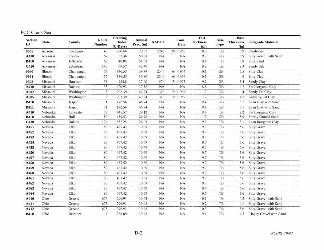
D-2 NCHRP 10-82

PCC Crack Seal

Section ID

State County Route

Number

Freezing Index

(C-Days)

Annual Prec. (in)

AADTT Cons. Date

PCC Thickness

(in)

Base Type

Base Thickness


0605 Arizona Coconino 40 260.66 20.67 2240 9/1/1966 8.3 TB 3.9 Sandstone A410 Arkansas Lonoke 67 52.36 50.08 NA NA 9.7 GB 3.9 Silty Gravel with Sand

B410 Arkansas Jefferson 65 40.05 51.53 NA NA 9.4 TB 6.9 Silty Sand

C410 Arkansas Sebastian 540 59.57 43.40 NA NA 9.3 TB 8.3 Sandy Silt

0660 Illinois Champaign 57 346.55 39.89 2340 6/1/1964 10.1 GB 7.5 Silty Clay

0661 Illinois Champaign 57 346.55 39.89 2340 6/1/1964 10.1 GB 8 Silty Clay

0602 Missouri Harrison 35 424.8 37.40 1570 7/1/1975 9.2 GB 3.4 Sandy Clay

A410 Missouri Daviess 35 420.93 37.38 NA NA 8.8 GB 4.2 Fat Inorganic Clay



B410 Missouri Jasper 71 172.56 46.74 NA NA 9.4 GB 3.5 Lean Clay with Sand

B411 Missouri Jasper 71 172.56 46.74 NA NA 9.4 GB 3.5 Lean Clay with Sand

A410 Nebraska Lancaster 77 445.57 29.12 NA NA 8.4 TB 2.2 Fat Inorganic Clay B410 Nebraska Hall 80 459.53 26.76 NA NA 12 GB 5.9 Poorly Graded Sand

C410 Nebraska Dakota 129 652.25 26.03 NA NA 9.2 TB 3.1 Lean Inorganic Clay

A451 Nevada Elko 80 467.42 10.69 NA NA 9.7 TB 5.6 Silty Gravel














A410 Ohio Greene 675 296.91 39.43 NA NA 10.1 TB 4.2 Silty Gravel with Sand



B410 Ohio Belmont 7 286.09 39.08 NA NA 9.1 TB 4.5 Clayey Gravel with Sand

D-3 NCHRP 10-82

Section ID

State County Route

Number

Freezing Index

(C-Days)

Annual Prec. (in)

AADTT Cons. Date

PCC Thickness

(in)

Base Type

Base Thickness


B411 Ohio Belmont 7 286.09 39.08 NA NA 9.1 TB 4.3 Clayey Gravel with Sand

B412 Ohio Belmont 7 286.09 39.08 NA NA 9 TB 4.2 Clayey Gravel with Sand

A410 Oklahoma Pontotoc 3W 64.17 40.35 NA NA 9.2 TB 2.2 Lean Clay with Sand


A410 Pennsylvania Lycoming 180 308.92 42.72 NA NA 10.5 GB 12 Gravelly Silt with Sand



A410 Texas Dallas 348 21.32 35.58 NA NA 9.3 TB 3.5 Fat Inorganic Clay

A420 Texas Dallas 348 21.32 35.58 NA NA 9.3 TB 3.5 Fat Inorganic Clay

B410 Texas Jefferson 90 2.35 57.66 NA NA 10.4 TB 4.3 Lean Inorganic Clay

B420 Texas Jefferson 90 2.35 57.66 NA NA 10 TB 4.3 Lean Inorganic Clay

C410 Texas Wilbarger 287 49.87 26.85 NA NA 10 GB 6.2 Silty Sand

C420 Texas Wilbarger 287 49.87 26.85 NA NA 10 GB 6.2 Silty Sand

D410 Texas Liberty 146 2.84 57.28 NA NA 11.4 TB 6.4 Sandy Silt D420 Texas Liberty 146 2.84 57.28 NA NA 11.4 TB 6.4 Sandy Silt E410 Texas Jasper 96 7.31 60.39 NA NA 9.6 TB 7.6 Clayey Sand E420 Texas Jasper 96 7.31 60.39 NA NA 9.6 TB 7.6 Clayey Sand

D410 Utah Salt Lake 154 192.87 17.59 NA NA 10.1 TB 5.4 Clayey Gravel with Sand












E445 Utah Wasatch 40 445.33 19.24 NA NA 9.7 TB 4.8 Silty Gravel with Sand






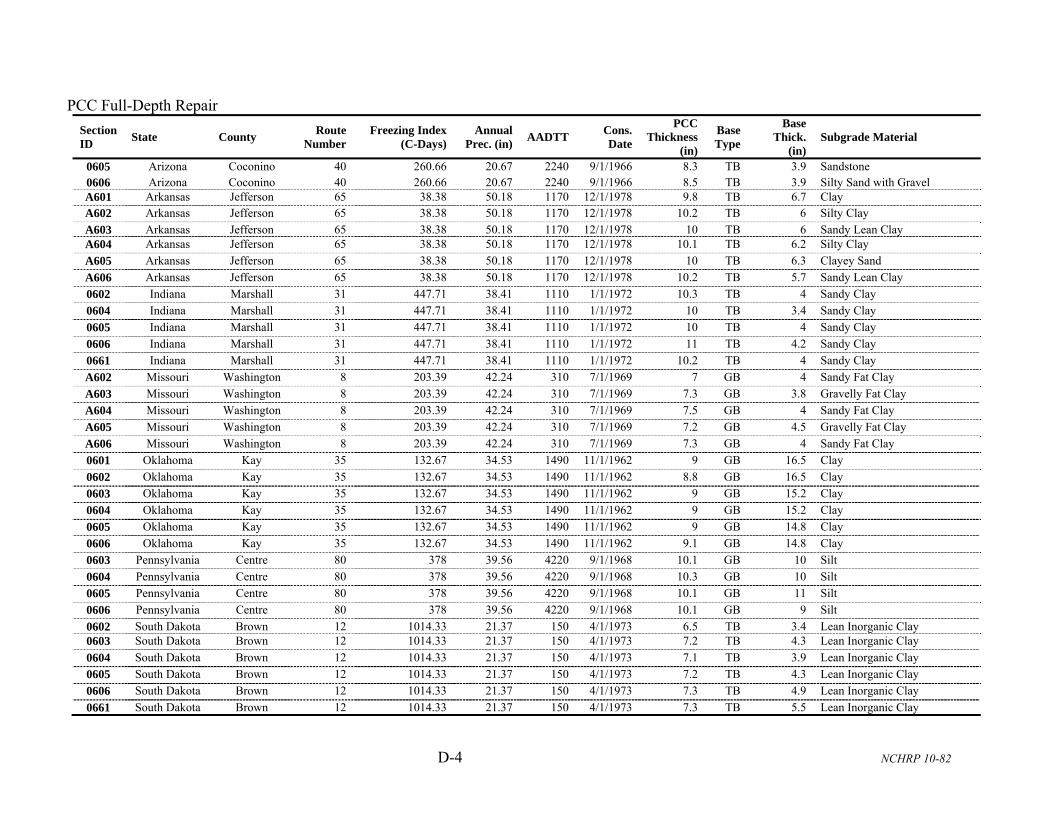
D-4 NCHRP 10-82

PCC Full-Depth Repair

Section ID

State County Route

Number Freezing Index

(C-Days) Annual

Prec. (in) AADTT

Cons. Date

PCC Thickness

(in)

Base Type

Base Thick.


0605 Arizona Coconino 40 260.66 20.67 2240 9/1/1966 8.3 TB 3.9 Sandstone 0606 Arizona Coconino 40 260.66 20.67 2240 9/1/1966 8.5 TB 3.9 Silty Sand with Gravel A601 Arkansas Jefferson 65 38.38 50.18 1170 12/1/1978 9.8 TB 6.7 Clay A602 Arkansas Jefferson 65 38.38 50.18 1170 12/1/1978 10.2 TB 6 Silty Clay

A603 Arkansas Jefferson 65 38.38 50.18 1170 12/1/1978 10 TB 6 Sandy Lean Clay A604 Arkansas Jefferson 65 38.38 50.18 1170 12/1/1978 10.1 TB 6.2 Silty Clay


A606 Arkansas Jefferson 65 38.38 50.18 1170 12/1/1978 10.2 TB 5.7 Sandy Lean Clay

0602 Indiana Marshall 31 447.71 38.41 1110 1/1/1972 10.3 TB 4 Sandy Clay

0604 Indiana Marshall 31 447.71 38.41 1110 1/1/1972 10 TB 3.4 Sandy Clay

0605 Indiana Marshall 31 447.71 38.41 1110 1/1/1972 10 TB 4 Sandy Clay





A604 Missouri Washington 8 203.39 42.24 310 7/1/1969 7.5 GB 4 Sandy Fat Clay


A606 Missouri Washington 8 203.39 42.24 310 7/1/1969 7.3 GB 4 Sandy Fat Clay











0602 South Dakota Brown 12 1014.33 21.37 150 4/1/1973 6.5 TB 3.4 Lean Inorganic Clay 0603 South Dakota Brown 12 1014.33 21.37 150 4/1/1973 7.2 TB 4.3 Lean Inorganic Clay





D-5 NCHRP 10-82


Section ID

State County Route

Number

Freezing Index

(C-Days)

Annual Prec. (in)

AADTT Cons. Date

PCC Thickness

(in)

Base Type

Base Thickness

(in)

Subgrade Material

A601 Arkansas Jefferson 65 38.38 50.18 1170 12/1/1978 9.8 TB 6.7 Clay

A602 Arkansas Jefferson 65 38.38 50.18 1170 12/1/1978 10.2 TB 6 Silty Clay

A603 Arkansas Jefferson 65 38.38 50.18 1170 12/1/1978 10 TB 6 Sandy Lean Clay

A604 Arkansas Jefferson 65 38.38 50.18 1170 12/1/1978 10.1 TB 6.2 Silty Clay






Underseal

Section ID

State County Route


(C-Days) Annual

Prec. (in) AADTT

Cons. Date

PCC Thickness

(in)

Base Type

Base Thickness


A421 California San Diego 8 0.62 15.10 NA NA 8.1 TB 5.4 Silty Sand with Gravel

A423 California San Diego 8 0.62 15.10 NA NA 8.1 TB 5.4 Silty Sand with Gravel

B421 California San Joaquin 5 0.36 12.10 NA NA 11.7 TB 4.8 Clayey Gravel with Sand

B423 California San Joaquin 5 0.36 12.10 NA NA 11.7 TB 4.8 Clayey Gravel with Sand


B420 Texas Jefferson 90 2.35 57.66 NA NA 10 TB 4.3 Lean Inorganic Clay

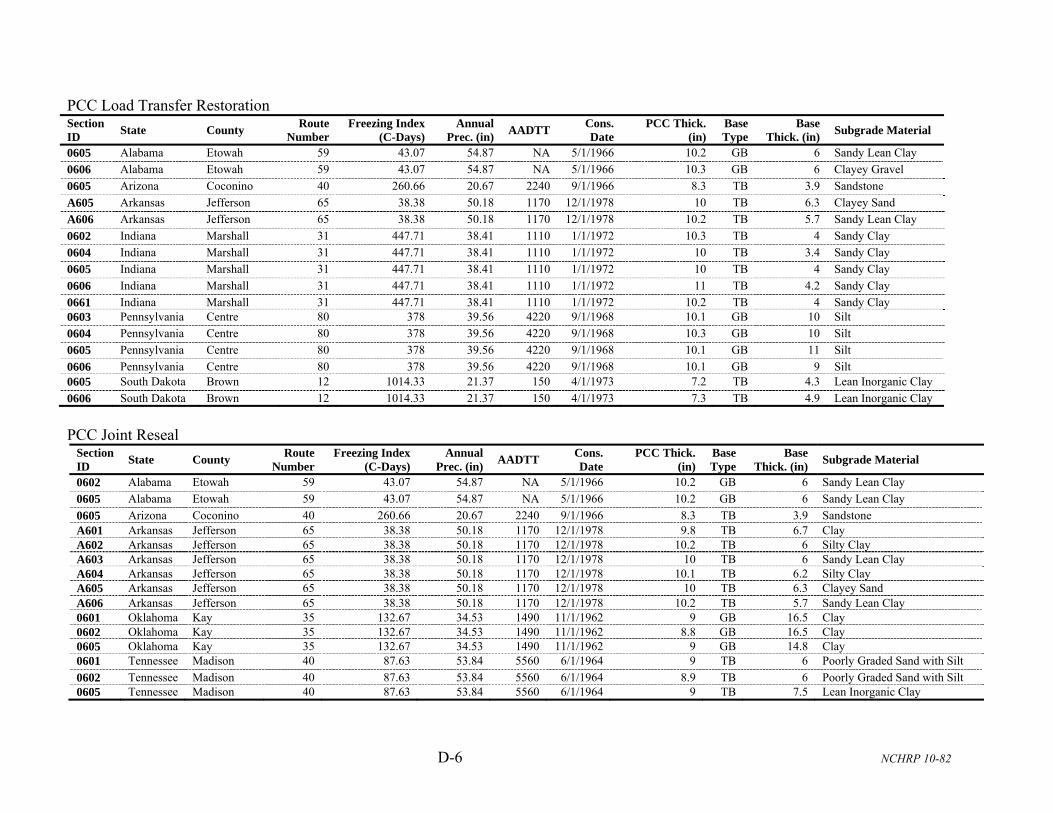
D-6 NCHRP 10-82

PCC Load Transfer Restoration Section ID

State County Route


(C-Days) Annual

Prec. (in) AADTT

Cons. Date

PCC Thick. (in)

Base Type

Base Thick. (in)

Subgrade Material


0606 Alabama Etowah 59 43.07 54.87 NA 5/1/1966 10.3 GB 6 Clayey Gravel

0605 Arizona Coconino 40 260.66 20.67 2240 9/1/1966 8.3 TB 3.9 Sandstone





0605 Indiana Marshall 31 447.71 38.41 1110 1/1/1972 10 TB 4 Sandy Clay


0661 Indiana Marshall 31 447.71 38.41 1110 1/1/1972 10.2 TB 4 Sandy Clay 0603 Pennsylvania Centre 80 378 39.56 4220 9/1/1968 10.1 GB 10 Silt



0606 Pennsylvania Centre 80 378 39.56 4220 9/1/1968 10.1 GB 9 Silt 0605 South Dakota Brown 12 1014.33 21.37 150 4/1/1973 7.2 TB 4.3 Lean Inorganic Clay


PCC Joint Reseal

Section ID

State County Route


(C-Days) Annual

Prec. (in) AADTT

Cons. Date

PCC Thick. (in)

Base Type

Base Thick. (in)

Subgrade Material



0605 Arizona Coconino 40 260.66 20.67 2240 9/1/1966 8.3 TB 3.9 Sandstone A601 Arkansas Jefferson 65 38.38 50.18 1170 12/1/1978 9.8 TB 6.7 Clay A602 Arkansas Jefferson 65 38.38 50.18 1170 12/1/1978 10.2 TB 6 Silty Clay A603 Arkansas Jefferson 65 38.38 50.18 1170 12/1/1978 10 TB 6 Sandy Lean Clay A604 Arkansas Jefferson 65 38.38 50.18 1170 12/1/1978 10.1 TB 6.2 Silty Clay A605 Arkansas Jefferson 65 38.38 50.18 1170 12/1/1978 10 TB 6.3 Clayey Sand A606 Arkansas Jefferson 65 38.38 50.18 1170 12/1/1978 10.2 TB 5.7 Sandy Lean Clay 0601 Oklahoma Kay 35 132.67 34.53 1490 11/1/1962 9 GB 16.5 Clay 0602 Oklahoma Kay 35 132.67 34.53 1490 11/1/1962 8.8 GB 16.5 Clay 0605 Oklahoma Kay 35 132.67 34.53 1490 11/1/1962 9 GB 14.8 Clay 0601 Tennessee Madison 40 87.63 53.84 5560 6/1/1964 9 TB 6 Poorly Graded Sand with Silt

0602 Tennessee Madison 40 87.63 53.84 5560 6/1/1964 8.9 TB 6 Poorly Graded Sand with Silt 0605 Tennessee Madison 40 87.63 53.84 5560 6/1/1964 9 TB 7.5 Lean Inorganic Clay

to the N C H R PROGRAM (NCHRP) - Transportation...

Documents

Transcript of to the N C H R PROGRAM (NCHRP) - Transportation...