To the Graduate Council: Mongi A. Abidi Major Professor · To the Graduate Council: I am submitting...
170
To the Graduate Council: I am submitting herewith a thesis written by Nikhil Arun Naik entitled “ Design, Development and Characterization of a Thermal Sensor Brick System for Modular Robotics.” I have examined the final electronic copy of this thesis for form and content and recommend that it be accepted in partial fulfillment of the requirements for the degree of Master of Science, with a major in Electrical Engineering. Mongi A. Abidi Major Professor We have read this thesis and recommend its acceptance: David L. Page Michael J. Roberts Accepted for the Council: Anne Mayhew Vice Chancellor and Dean of Graduate Studies (Original signatures are on file with official student records.)
Transcript of To the Graduate Council: Mongi A. Abidi Major Professor · To the Graduate Council: I am submitting...

To the Graduate Council: I am submitting herewith a thesis written by Nikhil Arun Naik entitled “Design, Development and Characterization of a Thermal Sensor Brick System for Modular Robotics.” I have examined the final electronic copy of this thesis for form and content and recommend that it be accepted in partial fulfillment of the requirements for the degree of Master of Science, with a major in Electrical Engineering.
Mongi A. Abidi
Major Professor We have read this thesis and recommend its acceptance:
David L. Page
Michael J. Roberts
Accepted for the Council:
Anne Mayhew Vice Chancellor and Dean of Graduate Studies
(Original signatures are on file with official student records.)
Design, Development and Characterization of a Thermal Sensor Brick System for Modular Robotics
A Thesis
Presented For The
Master of Science Degree
The University Of Tennessee, Knoxville
Nikhil Arun Naik
December 2006

ii
Copyright © 2006 Nikhil Arun Naik. All rights reserved.

iii
Dedication
I would like to dedicate this thesis to my parents Mr. Arun B. Naik and Mrs. Rati A. Naik for having encouraged me to pursue my Master’s degree. They have always been the pillars of support and encouragement throughout my life and have always laid stress on education and good values to make me a better individual.
iv
Acknowledgement
First of all I would like to thank my parents Mr. Arun B. Naik and Mrs. Rati A. Naik for having given me this opportunity to pursue my Master’s degree. They have always backed me in all my academic endeavors and I am highly indebted to them. I would sincerely like to thank my professor Dr. Mongi A. Abidi for his moral, academic and financial support during my Master’s study here at the University of Tennessee. Thank you for showing faith in my abilities and in giving me an opportunity, without you it would not have been possible for me to achieve my goals. Secondly I would like to thank Dr. David Page for his guidance during the second half of my Master’s work. He helped me in improving on my weaknesses and honing already existing skills. He also helped in inculcating the values of professionalism in me. Thank you for spending your valuable research time with me. I would like to thank Dr. Laura Morris Edwards for her sincere support to my research work at the IRIS laboratory during the formative stages. I would like to thank Dr. Andrei Gribok for helping me with the compilation of my PILOT report. He spent his valuable time in guiding me during that semester. I would like to thank Dr. Seong G. Kong and Dr. Michael J. Roberts for agreeing to be part of my graduate committee. I also want to thank Dr. Besma Abidi for valuable feedback and interactive discussions at research meetings. I would like to thank Justin Acuff for his sincere help with all the computer related technicalities involved with my Master’s work. I admire his hard working nature. My sincere thanks to Doug Warren for helping me in accomplishing the hardware related goals of my Master’s work. He has been my guide on the machining part of my Master’s work. I would also like to acknowledge Vicky Courtney Smith, Kim Kate, Sharon Foy, Diane Strutz and Robert Kadunce for their moral support. Finally I would like to thank all my friends at the IRIS laboratory, at the department, at my apartment complex, and all others that I have met and known in Knoxville. Thank you very much you all for making me feel special and very much at home. Special thanks to UT Transportation Department and all its work force for being kind and considerate in allowing us to use their facilities for our under vehicle experiments, it was fun interacting with them.
v
Abstract
This thesis presents the work on thermal imaging sensor brick (TISB) system for modular robotics. The research demonstrates the design, development and characterization of the TISB system. The TISB system is based on the design philosophy of sensor bricks for modular robotics. In under vehicle surveillance for threat detection, which is a target application of this work we have demonstrated the advantages of the TISB system over purely vision-based systems. We have highlighted the advantages of the TISB system as an illumination invariant threat detection system for detecting hidden threat objects in the undercarriage of a car. We have compared the TISB system to the vision sensor brick system and the mirror on a stick. We have also illustrated the operational capability of the system on the SafeBot under vehicle robot to acquire and transmit the data wirelessly. The early designs of the TISB system, the evolution of the designs and the uniformity achieved while maintaining the modularity in building the different sensor bricks; the visual, the thermal and the range sensor brick is presented as part of this work. Each of these sensor brick systems designed and implemented at the Imaging Robotics and Intelligent Systems (IRIS) laboratory consist of four major blocks: Sensing and Image Acquisition Block, Pre-Processing and Fusion Block, Communication Block, and Power Block. The Sensing and Image Acquisition Block is to capture images or acquire data. The Pre-Processing and Fusion Block is to work on the acquired images or data. The Communication Block is for transferring data between the sensor brick and the remote host computer. The Power Block is to maintain power supply to the entire brick. The modular sensor bricks are self-sufficient plug and play systems. The SafeBot under vehicle robot designed and implemented at the IRIS laboratory has two tracked platforms one on each side with a payload bay area in the middle. Each of these tracked platforms is a mobility brick based on the same design philosophy as the modular sensor bricks. The robot can carry one brick at a time or even multiple bricks at the same time. The contributions of this thesis are: (1) designing and developing the hardware implementation of the TISB system, (2) designing and developing the software for the TISB system, and (3) characterizing the TISB system, where this characterization of the system is the major contribution of this thesis. The analysis of the thermal sensor brick system provides the user and future designers with sufficient information on parameters to be considered to make the right choice for future modifications, the kind of applications the TISB could handle and the load that the different blocks of the TISB system could manage. Under vehicle surveillance for threat detection, perimeter / area surveillance, scouting, and improvised explosive device (IED) detection using a car-mounted system are some of the applications that have been identified for this system.

vi
Table of Contents
1 Introduction .....................................................................................................................1 1.1 Motivation and Overview ....................................................................................... 1 1.2 Mission.................................................................................................................... 5 1.3 Applications ............................................................................................................ 6 1.4 Contributions........................................................................................................... 8 1.5 Document Outline................................................................................................. 10
2 Literature Review..........................................................................................................11 2.1 Theory of Thermal Imaging...................................................................................11 2.2 Previous Work....................................................................................................... 18 2.3 Competing Technologies....................................................................................... 24
3 Hardware Architecture ..................................................................................................34 3.1 Sensing and Image Acquisition Block .................................................................. 35 3.2 Pre-Processing and Fusion Block ......................................................................... 40 3.3 Communication Block .......................................................................................... 40 3.4 Power Block.......................................................................................................... 43 3.5 Sensor Brick Design.............................................................................................. 46
4 Software Architecture ...................................................................................................53 4.1 Acquisition............................................................................................................ 53 4.2 Processing ............................................................................................................. 60 4.3 Interpretation......................................................................................................... 68
5 Characterization & Experimental Results.....................................................................70 5.1 Hardware Experiments.......................................................................................... 70 5.2 Scenario Experiments ......................................................................................... 125
6 Conclusions .................................................................................................................141 6.1 Summary ............................................................................................................. 141 6.2 Contributions....................................................................................................... 141 6.3 Lessons Learned.................................................................................................. 141 6.4 Future Work ........................................................................................................ 142
References .......................................................................................................................143 Appendices......................................................................................................................149
Appendix A: Modular Sensor Bricks ........................................................................ 150 Vita ..............................................................................................................................156
vii
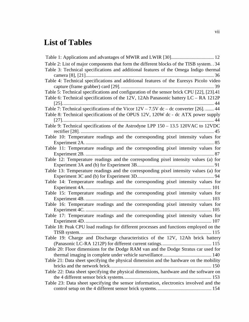
List of Tables
Table 1: Applications and advantages of MWIR and LWIR [30]................................... 12
Table 2: List of major components that form the different blocks of the TISB system. . 34 Table 3: Technical specifications and additional features of the Omega Indigo thermal
camera [8], [21]......................................................................................................... 36 Table 4: Technical specifications and additional features of the Euresys Picolo video
capture (frame grabber) card [29]. ............................................................................ 39 Table 5: Technical specifications and configuration of the sensor brick CPU [22], [23].41 Table 6: Technical specifications of the 12V, 12Ah Panasonic battery LC – RA 1212P
[25]............................................................................................................................ 44 Table 7: Technical specifications of the Vicor 12V – 7.5V dc – dc converter [26]. ....... 44 Table 8: Technical specifications of the OPUS 12V, 120W dc - dc ATX power supply
[27]............................................................................................................................ 44 Table 9: Technical specifications of the Astrodyne LPP 150 – 13.5 120VAC to 12VDC
rectifier [28]. ............................................................................................................. 45 Table 10: Temperature readings and the corresponding pixel intensity values for
Experiment 2A. ......................................................................................................... 85 Table 11: Temperature readings and the corresponding pixel intensity values for
Experiment 2B. ......................................................................................................... 87 Table 12: Temperature readings and the corresponding pixel intensity values (a) for
Experiment 3A and (b) for Experiment 3B............................................................... 91 Table 13: Temperature readings and the corresponding pixel intensity values (a) for
Experiment 3C and (b) for Experiment 3D............................................................... 94 Table 14: Temperature readings and the corresponding pixel intensity values for
Experiment 4A. ....................................................................................................... 101 Table 15: Temperature readings and the corresponding pixel intensity values for
Experiment 4B. ....................................................................................................... 103 Table 16: Temperature readings and the corresponding pixel intensity values for
Experiment 4C. ....................................................................................................... 105 Table 17: Temperature readings and the corresponding pixel intensity values for
Experiment 4D. ....................................................................................................... 107 Table 18: Peak CPU load readings for different processes and functions employed on the
TISB system............................................................................................................ 115 Table 19: Charge and Discharge characteristics of the 12V, 12Ah brick battery
(Panasonic LC-RA 1212P) for different current ratings......................................... 115 Table 20: Floor dimensions for the Dodge RAM van and the Dodge Stratus car used for
thermal imaging in complete under vehicle surveillance........................................ 140 Table 21: Data sheet specifying the physical dimension and the hardware on the mobility
bricks and the network brick................................................................................... 150 Table 22: Data sheet specifying the physical dimensions, hardware and the software on
the 4 different sensor brick systems........................................................................ 153 Table 23: Data sheet specifying the sensor information, electronics involved and the
control setup on the 4 different sensor brick systems. ............................................ 154
viii
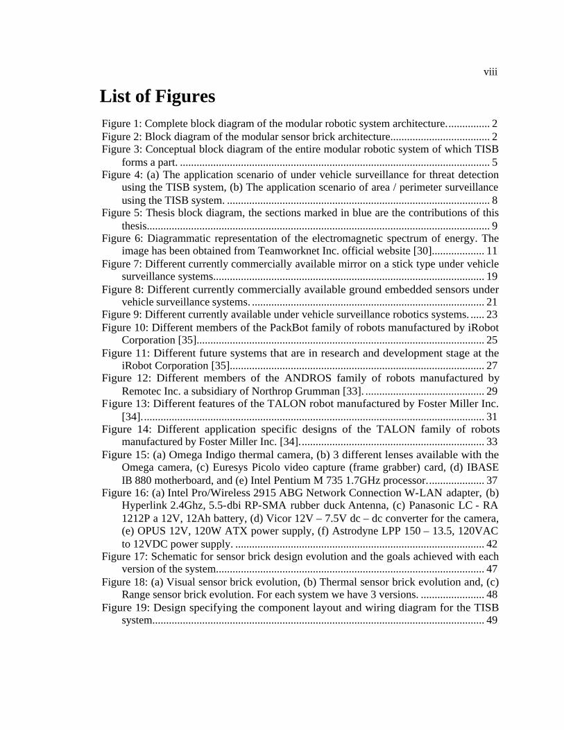
List of Figures
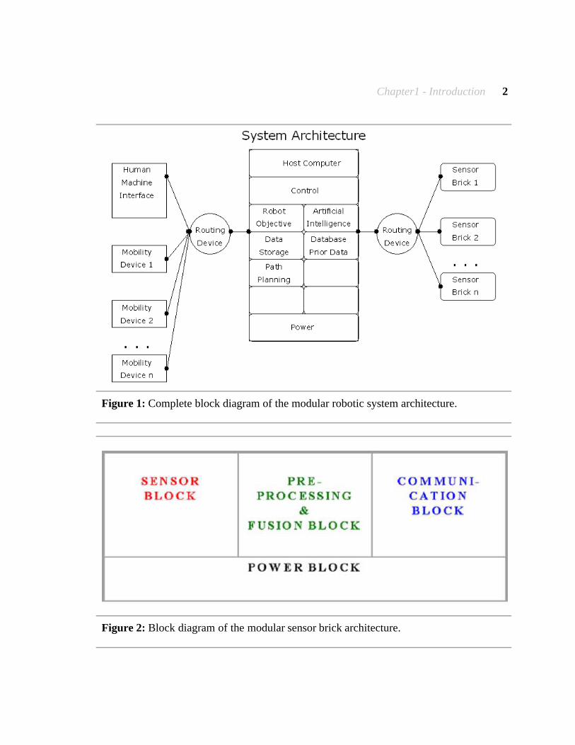
Figure 1: Complete block diagram of the modular robotic system architecture................ 2 Figure 2: Block diagram of the modular sensor brick architecture.................................... 2 Figure 3: Conceptual block diagram of the entire modular robotic system of which TISB
forms a part. ................................................................................................................ 5 Figure 4: (a) The application scenario of under vehicle surveillance for threat detection
using the TISB system, (b) The application scenario of area / perimeter surveillance using the TISB system. ............................................................................................... 8
Figure 5: Thesis block diagram, the sections marked in blue are the contributions of this thesis............................................................................................................................ 9
Figure 6: Diagrammatic representation of the electromagnetic spectrum of energy. The image has been obtained from Teamworknet Inc. official website [30]................... 11
Figure 7: Different currently commercially available mirror on a stick type under vehicle surveillance systems.................................................................................................. 19
Figure 8: Different currently commercially available ground embedded sensors under vehicle surveillance systems. .................................................................................... 21
Figure 9: Different currently available under vehicle surveillance robotics systems. ..... 23 Figure 10: Different members of the PackBot family of robots manufactured by iRobot
Corporation [35]........................................................................................................ 25 Figure 11: Different future systems that are in research and development stage at the
iRobot Corporation [35]............................................................................................ 27 Figure 12: Different members of the ANDROS family of robots manufactured by
Remotec Inc. a subsidiary of Northrop Grumman [33]. ........................................... 29 Figure 13: Different features of the TALON robot manufactured by Foster Miller Inc.
[34]............................................................................................................................ 31 Figure 14: Different application specific designs of the TALON family of robots
manufactured by Foster Miller Inc. [34]................................................................... 33 Figure 15: (a) Omega Indigo thermal camera, (b) 3 different lenses available with the
Omega camera, (c) Euresys Picolo video capture (frame grabber) card, (d) IBASE IB 880 motherboard, and (e) Intel Pentium M 735 1.7GHz processor..................... 37
Figure 16: (a) Intel Pro/Wireless 2915 ABG Network Connection W-LAN adapter, (b) Hyperlink 2.4Ghz, 5.5-dbi RP-SMA rubber duck Antenna, (c) Panasonic LC - RA 1212P a 12V, 12Ah battery, (d) Vicor 12V – 7.5V dc – dc converter for the camera, (e) OPUS 12V, 120W ATX power supply, (f) Astrodyne LPP 150 – 13.5, 120VAC to 12VDC power supply. .......................................................................................... 42
Figure 17: Schematic for sensor brick design evolution and the goals achieved with each version of the system................................................................................................. 47
Figure 18: (a) Visual sensor brick evolution, (b) Thermal sensor brick evolution and, (c) Range sensor brick evolution. For each system we have 3 versions. ....................... 48
Figure 19: Design specifying the component layout and wiring diagram for the TISB system........................................................................................................................ 49
ix
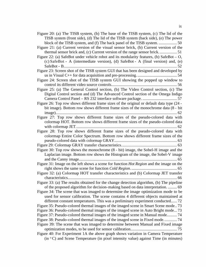
Figure 20: (a) The TISB system, (b) The base of the TISB system, (c) The lid of the TISB system (front side), (d) The lid of the TISB system (back side), (e) The power block of the TISB system, and (f) The back panel of the TISB system. .................. 50
Figure 21: (a) Current version of the visual sensor brick, (b) Current version of the thermal sensor brick and, (c) Current version of the range sensor brick. ................. 51
Figure 22: (a) SafeBot under vehicle robot and its modularity features, (b) SafeBot – O, (c) SafeBot - A (intermediate version), (d) SafeBot - A (final version) and, (e) SafeBot - B................................................................................................................ 52
Figure 23: Screen shot of the TISB system GUI that has been designed and developed by us in Visual C++ for data acquisition and pre-processing. ....................................... 54
Figure 24: Screen shot of the TISB system GUI showing the popped up window to control its different video source controls................................................................. 56
Figure 25: (a) The General Control section, (b) The Video Control section, (c) The Digital Control section and (d) The Advanced Control section of the Omega Indigo Camera Control Panel – RS 232 interface software package. .................................. 57
Figure 26: Top row shows different frame sizes of the original or default data type (24 - bit image). Bottom row shows different frame sizes of the monochrome data (8 - bit image)........................................................................................................................ 62
Figure 27: Top row shows different frame sizes of the pseudo-colored data with colormap HOT. Bottom row shows different frame sizes of the pseudo-colored data with colormap JET.................................................................................................... 62
Figure 28: Top row shows different frame sizes of the pseudo-colored data with colormap Entire Color Spectrum. Bottom row shows different frame sizes of the pseudo-colored data with colormap GRAY.............................................................. 63
Figure 29: Colormap GRAY transfer characteristics....................................................... 63 Figure 30: Top row shows the monochrome (8 - bit) image, the Sobel-H image and the
Laplacian image. Bottom row shows the Histogram of the image, the Sobel-V image and the Canny image................................................................................................. 65
Figure 31: Image on the left shows a scene for function Hot Region and the image on the right shows the same scene for function Cold Region. ............................................. 65
Figure 32: (a) Colormap HOT transfer characteristics and (b) Colormap JET transfer characteristics............................................................................................................ 66
Figure 33: (a) The results obtained for the change detection algorithm, (b) The pipeline of the proposed algorithm for decision-making based on data interpretation. ......... 69
Figure 34: The scene that was imaged to determine the image optimization mode to be used for sensor calibration. The scene contains 4 different objects maintained at different constant temperatures. This was a preliminary experiment conducted...... 72
Figure 35: Pseudo-colored thermal images of the imaged scene in Smart Scene mode.. 73 Figure 36: Pseudo-colored thermal images of the imaged scene in Auto Bright mode... 73 Figure 37: Pseudo-colored thermal images of the imaged scene in Manual mode.......... 74 Figure 38: Pseudo-colored thermal images of the imaged scene in Fixed mode............. 74 Figure 39: The scene that was imaged to determine between Manual and Fixed image
optimization modes, to be used for sensor calibration.............................................. 75 Figure 40: For Experiment 1A the above graph shows variation in Camera Temperature
(in °C) and Scene Temperature (in pixel intensity value) against Time (in minutes)

x
with following parameters kept constant: Mode = Manual, Contrast = 100, Brightness = 8428, Room Temp = 21.7°C. Camera was switched ON instantly and the scene was not fixed (with variations).................................................................. 76
Figure 41: The scene that was imaged to determine between Manual and Fixed image optimization modes, to be used for sensor calibration. This was a fixed scene with its temperature being monitored. ................................................................................... 78
Figure 42: For Experiment 1B the above graph shows variation in Camera Temperature (in °C) and Scene Temperature (in pixel intensity value) against Time (in minutes) with following parameters kept constant: Mode = Manual, Contrast = 100, Brightness = 8428, Room Temp = 20.3°C. Camera was switched ON instantly and the scene was fixed (no variations)........................................................................... 79
Figure 43: For Experiment 1C the above graph shows variation in Camera Temperature (in °C) and Scene Temperature (in pixel intensity value) against Time (in minutes) with following parameters kept constant: Mode = Fixed, Contrast = 100, Brightness = 8428, Room Temp = 20.6°C. Camera was switched ON instantly and the scene was fixed (no variations)........................................................................................... 80
Figure 44: For Experiment 1D the above graph shows variation in Camera Temperature (in °C) and Scene Temperature (in pixel intensity value) against Time (in minutes) with following parameters kept constant: Mode = Fixed, Contrast = 100, Brightness = 8428, Room Temp = 16°C. Camera was switched ON instantly and the scene was fixed (no variations).................................................................................................. 81
Figure 45: For Experiment 1E the above graph shows variation in Camera Temperature (in °C) and Scene Temperature (in pixel intensity value) against Time (in minutes) with following parameters kept constant: Mode = Fixed, Contrast = 100, Brightness = 8428, Room Temp = 18.6°C. The camera was switched ON for 2 hours before use and the scene was fixed (no variations). ................................................................... 83
Figure 46: For Experiment 2A the above graph shows variation in Temperature (in °C) and Temperature (in pixel intensity value) against Time (in minutes) for 4 different constant temperature sources. ................................................................................... 86
Figure 47: For Experiment 2B the above graph shows variation in Temperature (in °C) and Temperature (in pixel intensity value) against Time (in minutes) for 5 different constant temperature sources. ................................................................................... 88
Figure 48: Images (a), (b), (c) and (d) show the different setups used to for Experiment 3 A, B, C and D respectively to prove that image intensities from the thermal camera do not depend on the color of the object but instead depend directly on its temperature................................................................................................................ 90
Figure 49: For Experiment 3A the above graph shows variation in Temperature (in °C) and Temperature (in pixel intensity value) against Time (in minutes) for 2 different constant temperature sources as shown in Figure 48 (a). ......................................... 92
Figure 50: For Experiment 3B the above graph shows variation in Temperature (in °C) and Temperature (in pixel intensity value) against Time (in minutes) for 2 different constant temperature sources as shown in Figure 48 (b). ......................................... 93
xi
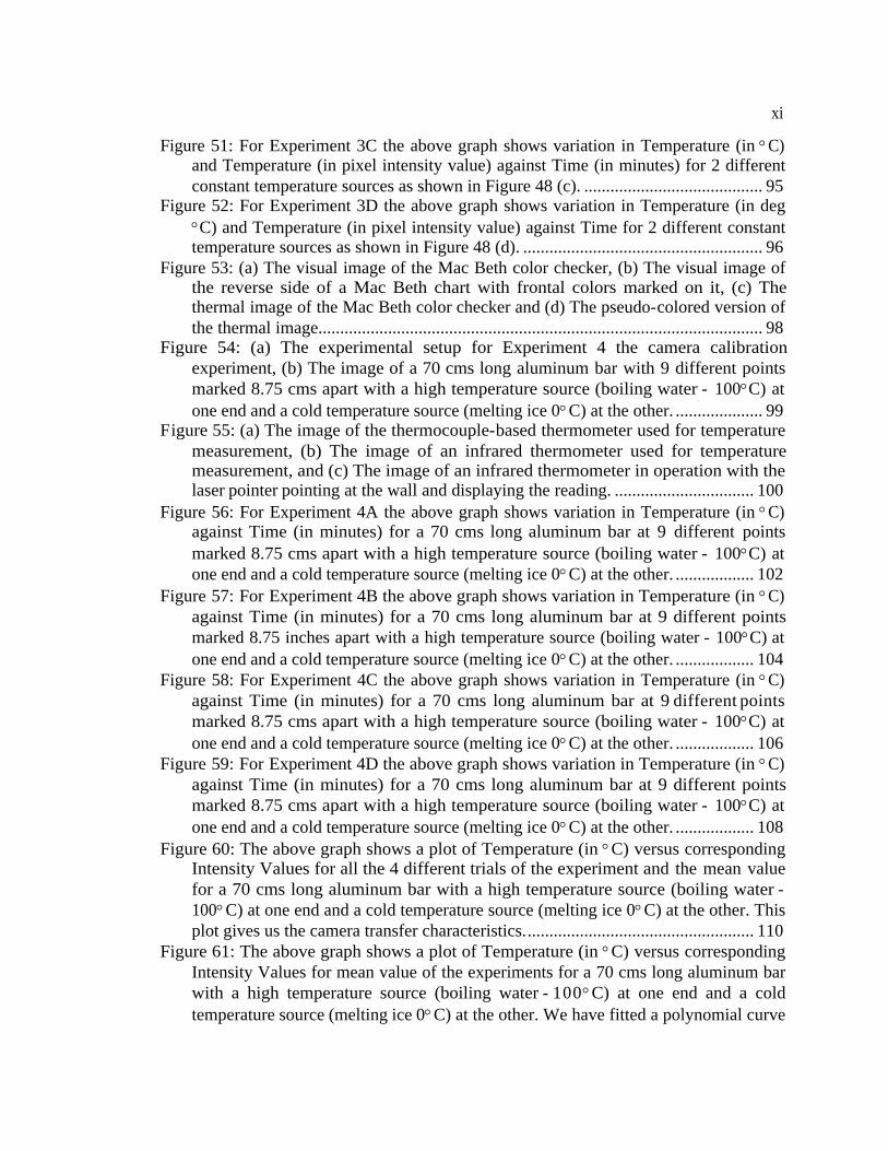
Figure 51: For Experiment 3C the above graph shows variation in Temperature (in °C) and Temperature (in pixel intensity value) against Time (in minutes) for 2 different constant temperature sources as shown in Figure 48 (c). ......................................... 95
Figure 52: For Experiment 3D the above graph shows variation in Temperature (in deg
°C) and Temperature (in pixel intensity value) against Time for 2 different constant temperature sources as shown in Figure 48 (d). ....................................................... 96
Figure 53: (a) The visual image of the Mac Beth color checker, (b) The visual image of the reverse side of a Mac Beth chart with frontal colors marked on it, (c) The thermal image of the Mac Beth color checker and (d) The pseudo-colored version of the thermal image...................................................................................................... 98
Figure 54: (a) The experimental setup for Experiment 4 the camera calibration experiment, (b) The image of a 70 cms long aluminum bar with 9 different points marked 8.75 cms apart with a high temperature source (boiling water - 100°C) at one end and a cold temperature source (melting ice 0°C) at the other. .................... 99
Figure 55: (a) The image of the thermocouple-based thermometer used for temperature measurement, (b) The image of an infrared thermometer used for temperature measurement, and (c) The image of an infrared thermometer in operation with the laser pointer pointing at the wall and displaying the reading. ................................ 100
Figure 56: For Experiment 4A the above graph shows variation in Temperature (in °C) against Time (in minutes) for a 70 cms long aluminum bar at 9 different points marked 8.75 cms apart with a high temperature source (boiling water - 100°C) at one end and a cold temperature source (melting ice 0°C) at the other. .................. 102
Figure 57: For Experiment 4B the above graph shows variation in Temperature (in °C) against Time (in minutes) for a 70 cms long aluminum bar at 9 different points marked 8.75 inches apart with a high temperature source (boiling water - 100°C) at one end and a cold temperature source (melting ice 0°C) at the other. .................. 104
Figure 58: For Experiment 4C the above graph shows variation in Temperature (in °C) against Time (in minutes) for a 70 cms long aluminum bar at 9 different points marked 8.75 cms apart with a high temperature source (boiling water - 100°C) at one end and a cold temperature source (melting ice 0°C) at the other. .................. 106
Figure 59: For Experiment 4D the above graph shows variation in Temperature (in °C) against Time (in minutes) for a 70 cms long aluminum bar at 9 different points marked 8.75 cms apart with a high temperature source (boiling water - 100°C) at one end and a cold temperature source (melting ice 0°C) at the other. .................. 108
Figure 60: The above graph shows a plot of Temperature (in °C) versus corresponding Intensity Values for all the 4 different trials of the experiment and the mean value for a 70 cms long aluminum bar with a high temperature source (boiling water - 100°C) at one end and a cold temperature source (melting ice 0°C) at the other. This plot gives us the camera transfer characteristics..................................................... 110
Figure 61: The above graph shows a plot of Temperature (in °C) versus corresponding Intensity Values for mean value of the experiments for a 70 cms long aluminum bar with a high temperature source (boiling water - 100°C) at one end and a cold temperature source (melting ice 0°C) at the other. We have fitted a polynomial curve
xii
using Microsoft Excel and MATLAB. This plot gives us the camera transfer equation................................................................................................................... 111
Figure 62: The above graph shows a plot of Temperature (in °C) versus Distance (in cms) of the measured point from boiling water for all the 4 different trials of the experiment for a 70 cms long aluminum bar with a high temperature source (boiling water - 100°C) at one end and a cold temperature source (melting ice 0°C) at the other. ....................................................................................................................... 112
Figure 63: The above graph shows a plot of Intensity Values versus Distance (in cms) of the measured point from boiling water for all the 4 different trials of the experiment for a 70 cms long aluminum bar with a high temperature source (boiling water - 100°C) at one end and a cold temperature source (melting ice 0°C) at the other... 113
Figure 64: Screen shot of the windows task manager, which shows CPU load of the system while processing data using colormaps. ..................................................... 116
Figure 65: Screen shot of the windows task manager, which shows CPU load of the system during edge detection and smoothing processing operations. .................... 117
Figure 66: Screen shot of the windows task manager, which shows CPU load of the system while processing data using morphological operations and then the load reduces as the GUI is closed and the system is idle................................................ 118
Figure 67: (a) Scaled plot of brick battery (Panasonic LC-RA 1212P) charge characteristics at 2A, (b) Full plot of brick battery (Panasonic LC-RA 1212P) charge characteristics at 2A................................................................................................ 119
Figure 68: (a) Full plot of brick battery (Panasonic LC-RA 1212P) charge characteristics at 10A, (b) Full plot of brick battery (Panasonic LC-RA 1212P) charge characteristics at 12A.............................................................................................. 120
Figure 69: (a) Scaled plot of brick battery (Panasonic LC-RA 1212P) charge characteristics at 20A, (b) Full plot of brick battery (Panasonic LC-RA 1212P) charge characteristics at 20A. ................................................................................. 121
Figure 70: Full plot of the combined brick battery (Panasonic LC-RA 1212P) charge characteristics, (2A, 10A, 12A, 20A)...................................................................... 122
Figure 71: (a) Scaled plot of brick battery (Panasonic LC-RA 1212P) discharge characteristics at 12 A, (b) Full plot of brick battery (Panasonic LC-RA 1212P) discharge characteristics at 12A.............................................................................. 123
Figure 72: (a) Full plot of brick battery (Panasonic LC-RA 1212P) discharge characteristics at 24 A, (b) Full plot of the combined brick battery (Panasonic LC-RA 1212P) discharge characteristics, (12A, 24A).................................................. 124
Figure 73: (a) Visual image of a section of the undercarriage of a van acquired using the visual imaging system, (b) Image of the same section as seen with the mirror on a stick, (c) Thermal image of the same section acquired using our TISB system, and (d) Pseudo-colored thermal image of the same section which highlights the cold object wrapped around a hot muffler. ..................................................................... 126
Figure 74: This under vehicle thermal video data was obtained to monitor variation in thermal conditions with time for an engine that has been running for 30 minutes, for each section we have the visual, the thermal and the pseudo-colored thermal image.................................................................................................................................. 127
xiii
Figure 75: This under vehicle thermal video data was obtained to check for expected results, for each section we have the visual, the thermal and the pseudo-colored thermal image.......................................................................................................... 128
Figure 76: This under vehicle thermal video data was obtained to check for normal results, for each section we have the visual, the thermal and the pseudo-colored thermal image.......................................................................................................... 129
Figure 77: (a), (b), (c) and (d) are different images of the Ford Taurus car, Dodge Stratus car and Dodge RAM 3500 van used for threat detection experiments in under vehicle surveillance. We can see the sensor brick mounted on the SafeBot under vehicle robot for inspection and is remotely (wirelessly) controlled by the user. .. 131
Figure 78: (a) View of the catalytic converter area for the Ford Taurus car, and (b) Same view with a hidden threat object behind it, for each view we have a visual image, a thermal image and a pseudo-colored thermal image. ............................................. 132
Figure 79: (a) View of the gas tank area for the Ford Taurus car, and (b) Same view with a hidden threat object behind it, for each view we have a visual image, a thermal image and a pseudo-colored thermal image............................................................ 133
Figure 80: (a) View of the muffler area for the Ford Taurus car, and (b) Same view with a hidden threat object behind it, for each view we have a visual image, a thermal image and a pseudo-colored thermal image............................................................ 134
Figure 81: (a) View of the muffler and axle area for the Dodge RAM van, and (b) Same view with a hidden threat object behind it, for each view we have a visual image, a thermal image and a pseudo-colored thermal image. ............................................. 135
Figure 82: (a) View of the exhaust manifold area for the Dodge RAM van, and (b) Same view with a hidden threat object behind it, for each view we have a visual image, a thermal image and a pseudo-colored thermal image. ............................................. 136
Figure 83: (a) View of the engine area for the Dodge RAM van, and (b) Same view with a hidden threat object behind it, for each view we have a visual image, a thermal image and a pseudo-colored thermal image............................................................ 137
Figure 84: (a) View of the gas tank and axle area for the Dodge RAM van, and (b) Same view with a hidden threat object behind it, for each view we have a visual image, a thermal image and a pseudo-colored thermal image. ............................................. 138
Figure 85: (a) View of an area at the rear end of the Dodge RAM van, and (b) Same view with a hidden threat object behind it, for each view we have a visual image, a thermal image and a pseudo-colored thermal image. ............................................. 139
Figure 86: Diagrammatic representation of the floor dimensions of the Dodge RAM 3500 van and Dodge Stratus car used for thermal imaging in complete under vehicle surveillance video sequences. ................................................................................. 140
Figure 87: Images of Range Sensor Brick, Thermal Sensor Brick and Visual Sensor Brick that have been implemented at the IRIS laboratory...................................... 151
Figure 88: Images of Nuclear Sensor Brick, SafeBot-O, SafeBot-A and SafeBot-B robots that have been implemented at the IRIS laboratory................................................ 152
Figure 89: The Modular robotic system with a central control computer, the 4 sensor bricks and the 2 robots communicating with each other and being controlled wirelessly for under vehicle surveillance................................................................ 155

Chapter1 - Introduction 1
1 Introduction
Research in the field of robotic systems has been going on for about half a century, but in the last fifteen to twenty years some progress has been made in the area of advanced robotics. Most robots that are available at the moment to the law enforcement authorities and other agencies for search and surveillance operations are either equipped with only one or two sensors (i.e. either the vision sensor and/or the radar or laser sensor). Also these sensors are usually fixed to the main system and are inseparable entities and cannot exist by themselves, and provide with little or no image or data processing capabilities. The sensor brick systems designed and developed at the IRIS laboratory are based on the philosophy of modular sensor bricks, which has been established here at the IRIS laboratory [6], [9], [10]. Each sensor brick consists of four blocks: Sensing and Image Acquisition Block, Pre-Processing and Fusion Block, Communication Block and Power Block. The sensor brick, which is like a plug and play device can thus exist either as a stand-alone system or as part of a multi sensor modular robotic setup and have image processing capabilities. The sensor bricks are both designed and built with main focus being set on its modularity and self-sufficiency. Since the sensor bricks are built as such highly modular systems, a setup like this allows the user to replace almost each and every major component in the system without affecting the remaining setup incase of damage to a working part or necessary upgrade due to technological advances. Figure 1 below shows the complete block diagram of the modular robotic system architecture, and Figure 2 below shows the block diagram of the modular sensor brick architecture. Each sensor brick is a building block of the overall modular robotic structure.
1.1 Motivation and Overview
The alarming rate at which both safety and security are proving to be a major cause for concern was the primary motivating factor for this project. The modular robotic system with four different kinds of sensors; the visual sensor brick, the thermal sensor brick, the range sensor brick and the neutron and gamma ray detection system along with the two mobile robotic platforms Safebot- A which can carry one sensor and SafeBot - B which can carry multiple sensors provide excellent capabilities for under vehicle search and surveillance operations. Other motivating factors being that a modular and flexible system allows for easy replacement and update of hardware and software. We can combine different kinds of sensors for data collection and data fusion. A modular system is one solution to the problem of designing, fabricating and testing cost-effective intelligent mobile robotic systems.
Chapter1 - Introduction 2
Figure 1: Complete block diagram of the modular robotic system architecture.
Figure 2: Block diagram of the modular sensor brick architecture.
Chapter1 - Introduction 3
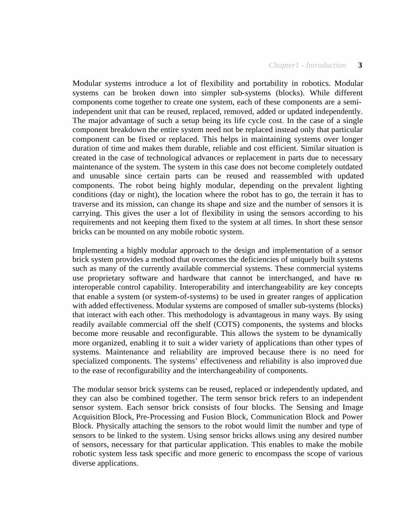
Modular systems introduce a lot of flexibility and portability in robotics. Modular systems can be broken down into simpler sub-systems (blocks). While different components come together to create one system, each of these components are a semi-independent unit that can be reused, replaced, removed, added or updated independently. The major advantage of such a setup being its life cycle cost. In the case of a single component breakdown the entire system need not be replaced instead only that particular component can be fixed or replaced. This helps in maintaining systems over longer duration of time and makes them durable, reliable and cost efficient. Similar situation is created in the case of technological advances or replacement in parts due to necessary maintenance of the system. The system in this case does not become completely outdated and unusable since certain parts can be reused and reassembled with updated components. The robot being highly modular, depending on the prevalent lighting conditions (day or night), the location where the robot has to go, the terrain it has to traverse and its mission, can change its shape and size and the number of sensors it is carrying. This gives the user a lot of flexibility in using the sensors according to his requirements and not keeping them fixed to the system at all times. In short these sensor bricks can be mounted on any mobile robotic system. Implementing a highly modular approach to the design and implementation of a sensor brick system provides a method that overcomes the deficiencies of uniquely built systems such as many of the currently available commercial systems. These commercial systems use proprietary software and hardware that cannot be interchanged, and have no interoperable control capability. Interoperability and interchangeability are key concepts that enable a system (or system-of-systems) to be used in greater ranges of application with added effectiveness. Modular systems are composed of smaller sub-systems (blocks) that interact with each other. This methodology is advantageous in many ways. By using readily available commercial off the shelf (COTS) components, the systems and blocks become more reusable and reconfigurable. This allows the system to be dynamically more organized, enabling it to suit a wider variety of applications than other types of systems. Maintenance and reliability are improved because there is no need for specialized components. The systems’ effectiveness and reliability is also improved due to the ease of reconfigurability and the interchangeability of components. The modular sensor brick systems can be reused, replaced or independently updated, and they can also be combined together. The term sensor brick refers to an independent sensor system. Each sensor brick consists of four blocks. The Sensing and Image Acquisition Block, Pre-Processing and Fusion Block, Communication Block and Power Block. Physically attaching the sensors to the robot would limit the number and type of sensors to be linked to the system. Using sensor bricks allows using any desired number of sensors, necessary for that particular application. This enables to make the mobile robotic system less task specific and more generic to encompass the scope of various diverse applications.

Chapter1 - Introduction 4
Many robotic platform based image-processing systems are currently available for both commercial and research operations. These robotic systems, which are available, are usually fitted with only one or two kinds of sensors (mostly cameras). The systems available are generally neither light in weight nor small in size and in case if any system is small in size and light in weight then it is highly improbable to be as highly sophisticated and modular as our sensor brick system. The systems also do not employ any on board processing capabilities and are usually tethered and have no or little wireless communication. Also the currently available systems are all equipped with expensive proprietary hardware and software components that are non-interchangeable. All the above characteristics contribute to the difficulties associated with interoperable control. In direct contrast to these systems, the modular sensor brick systems utilize sensor payloads that are easily interchangeable and require no special mounting system or equipment. By utilizing modular design, a component failure does not adversely affect the operational status of the system; an entire module consisting of COTS component, quickly and easily replaces the failed component in a plug-and-play capacity. Interoperability can also be more readily implemented with a modular designed system. In summary, modular sensor brick systems attempt to address some flaws of commercial systems, which are built for specific purposes, have no interoperable control capability, and the (sensor) payloads are not readily interchangeable. The above discussion helps us to a certain extent in getting a clearer picture about the possible advantages of our TISB system. Thermal imaging based robotic systems have been used previously in high- level rescue operations like in the case of rescue operation at the world trade center site. The robots used there were equipped with thermal cameras so that the body heat could be detected very easily. Robotic systems with thermal cameras have also been used to recover flight recorders of electronic aircraft data and voice recordings. So all in all, we know that the TISB system would be an important arm of any modular robotic platform meant for search and surveillance. It would help in giving vision beyond the human eyes and thereby help in overcoming the loopholes left in search and surveillance operations due to the limitations of a vision camera. The TISB system promises to be of great use in search and surveillance operations with its inherent advantages being that it is small in size and light in weight. Being able to capture thermal data is what makes it very special because in the dark where human vision stops the thermal sensor could be used to detect possible ambushes, plots and hidden threat objects underneath a vehicle by making use of its ability to generate thermal images which, highlight temperature disparities in the area that is being imaged. The thermal images generated could be used for under vehicle threat detection, they could also be used for obtaining a complete view of the under vehicle in the dark or in the absence of good lighting conditions as is generally the case underneath a vehicle. So to design, develop, test, demonstrate and enhance the capabilities of the TISB system was the main motivating factor for this project.
Chapter1 - Introduction 5
1.2 Mission
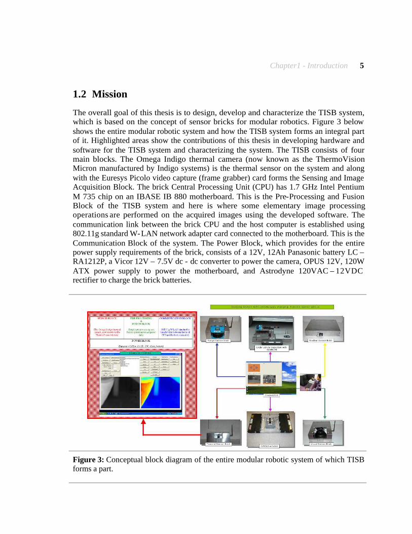
The overall goal of this thesis is to design, develop and characterize the TISB system, which is based on the concept of sensor bricks for modular robotics. Figure 3 below shows the entire modular robotic system and how the TISB system forms an integral part of it. Highlighted areas show the contributions of this thesis in developing hardware and software for the TISB system and characterizing the system. The TISB consists of four main blocks. The Omega Indigo thermal camera (now known as the ThermoVision Micron manufactured by Indigo systems) is the thermal sensor on the system and along with the Euresys Picolo video capture (frame grabber) card forms the Sensing and Image Acquisition Block. The brick Central Processing Unit (CPU) has 1.7 GHz Intel Pentium M 735 chip on an IBASE IB 880 motherboard. This is the Pre-Processing and Fusion Block of the TISB system and here is where some elementary image processing operations are performed on the acquired images using the developed software. The communication link between the brick CPU and the host computer is established using 802.11g standard W-LAN network adapter card connected to the motherboard. This is the Communication Block of the system. The Power Block, which provides for the entire power supply requirements of the brick, consists of a 12V, 12Ah Panasonic battery LC – RA1212P, a Vicor 12V – 7.5V dc - dc converter to power the camera, OPUS 12V, 120W ATX power supply to power the motherboard, and Astrodyne 120VAC – 12VDC rectifier to charge the brick batteries.
Figure 3: Conceptual block diagram of the entire modular robotic system of which TISB forms a part.

Chapter1 - Introduction 6
1.3 Applications
With extra impetus being given to security and safety issues in the past five years the TISB system finds many applications especially in search and surveillance operations. Having the system mounted on a manned or unmanned mobile robotic system it could aid to protect human beings from probable or anticipated danger. Security based applications are more suited to the needs of organizations like the Department Of Energy (DOE) and Department of Homeland Security (DHS). The Automotive Research Center (ARC), which develops simulations and designs for mobile platforms to be applicable in real world environments could also benefit from the use of TISB system for scanning processes and multi-sensor data acquisition. We shall look at some of the possible applications of the system in general and then we shall deal with four applications in some detail. From the search, surveillance and security perspective some of the scenarios where the TISB system could be of use are: Under vehicle Surveillance, Area / Perimeter Surveillance, Scouting Missions, Checkpoint Inspections, Intrusion Detection. Border Crossing Inspection, Customs Inspection, Stadiums, Power Plants, Chemical Plants, Nuclear Plants, Petroleum Refinery’s, Busy Parking Lots, Part of Search, Rescue, and Recovery Teams, Post-Event Inspection, Bridges, Landmarks, Tunnels, Hydroelectric Dams. In naval operations it could be used for detecting possible oil spillage and also threat from enemy vessels at night in the dark. In air force they could use it for aerial surveillance and enemy detection. Most of the above-mentioned applications of the TISB system would be of use in the military operations. The other possible applications could be in industrial production for quality control in the manufacturing process of a variety of products ranging from food items, glass, cast iron patterns, moulds and others where quality assurance of the product and surveillance on the production line is a necessity. The TISB could also be setup to guard secure locations where it would be expected to monitor entry and exit to a particular room or building by allowing only selected people to get in. It would accomplish the above task by using face recognition by thermal images to match new images with its current database. Some of the commercial applications would include coverage of disaster footages through smoke and dark areas, traffic reports even on a rainy and foggy day. When hooked up to a multi-sensor mobile robotic system the TISB could give the robot night vision to control its movement in the dark. The thermal images could also be used to thwart ambushes and plots laid in the dark by people directly or by using other objects or animals. Other primary applications of the TISB system could be in face recognition, pattern recognition and also perhaps in human tracking systems.

Chapter1 - Introduction 7
1.3.1 Under vehicle Surveillance
Under vehicle surveillance for threat detection is one of the major target applications of our modular robotics system. Currently security inspections of cars at entry gates and check points to check for bombs, threat objects and other unwanted contraband substances are conducted manually and maybe using a mirror on the stick. Scanning the undercarriage of a car using the mirror on a stick covers about 30% - 40% of the under carriage of a car, also the inspector has to be highly agile and runs the risk to his life being in close proximity to the car (possible threat). Using the TISB system mounted on the SafeBot under vehicle robot to scan the undercarriage of the car is a much more safer and efficient option. The thermal image shows us the hot and the cold parts of the undercarriage and if this does not meet our expectation then we know that we have a problem. People at the army have told us that some of the tricks that are used to sabotage are, to fix a false muffler along with the true muffler and imitate a dual exhaust system. The thermal image would spot this anomaly since false muffler would be cold. The TISB system is an illumination invariant threat detection system and can detect hidden threat objects in the undercarriage of the car even under poor lighting conditions. Figure 4 (a) demonstrates the application of TISB in the under vehicle inspection scenario.
1.3.2 Perimeter Surveillance
Safety and security are the main focus area of operations for the DOE and DHS. DOE deals with chemical safety, nuclear safety and hazardous waste transport. National Nuclear Safety Agency (NNSA), a semi-autonomous agency with the DOE could use the TISB system for Area surveillance. NNSA enhances national security through the military use of nuclear energy. As part of its task it develops and maintains nuclear weapons and also responds to nuclear and radiological emergencies in the USA and abroad. To prevent terrorists from accessing dangerous material, a robot equipped with a TISB system could perform area / perimeter surveillance and look for intruders or other anomalies. The National Safe Skies Administration (NSSA), which looks after all the airports in USA could also benefit from TISB for area / perimeter surveillance. Figure 4 (b) demonstrates the application of TISB in the perimeter area / surveillance scenario.
1.3.3 Scouting
When setup on a mobile robotic platform the TISB system could possibly help in scouting missions like in a building or in a nuclear reactor where it could be asked to detect leaks, fire, see through smoke and search for victims, detect for the presence of other flammable substances. Such an application is highly desirable especially in the case of agencies such as the Weapons of Mass Destruction Civilian Support Team. These military teams were established to protect U.S. citizens against the growing threat of chemical and biological terrorism. They are present in different states of the country to support federal and local agencies in the event of some incident involving weapons of mass destruction.
Chapter1 - Introduction 8
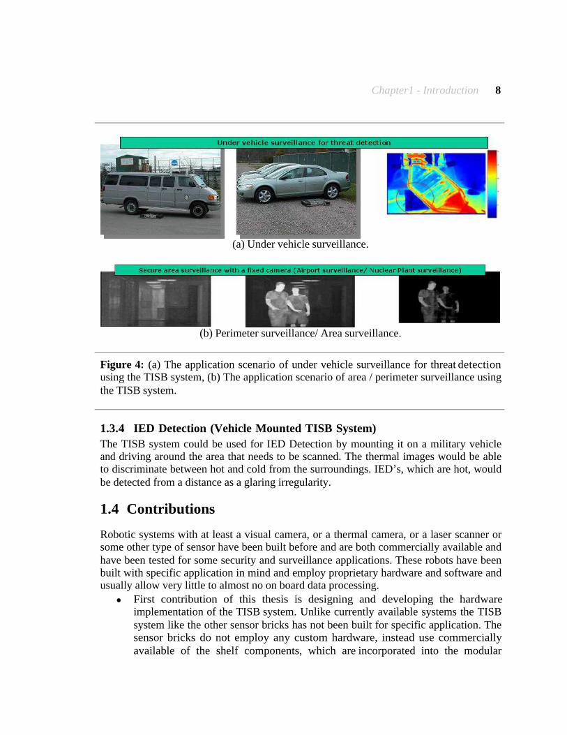
(a) Under vehicle surveillance.
(b) Perimeter surveillance/ Area surveillance.
Figure 4: (a) The application scenario of under vehicle surveillance for threat detection using the TISB system, (b) The application scenario of area / perimeter surveillance using the TISB system.
1.3.4 IED Detection (Vehicle Mounted TISB System)
The TISB system could be used for IED Detection by mounting it on a military vehicle and driving around the area that needs to be scanned. The thermal images would be able to discriminate between hot and cold from the surroundings. IED’s, which are hot, would be detected from a distance as a glaring irregularity.
1.4 Contributions
Robotic systems with at least a visual camera, or a thermal camera, or a laser scanner or some other type of sensor have been built before and are both commercially available and have been tested for some security and surveillance applications. These robots have been built with specific application in mind and employ proprietary hardware and software and usually allow very little to almost no on board data processing.
· First contribution of this thesis is designing and developing the hardware implementation of the TISB system. Unlike currently available systems the TISB system like the other sensor bricks has not been built for specific application. The sensor bricks do not employ any custom hardware, instead use commercially available of the shelf components, which are incorporated into the modular
Chapter1 - Introduction 9
design. The modular design makes the system more efficient, reliable and cost effective. The modular system is not rigid and section wise modifications of the robot are possible without affecting the entire system. All the sensor brick systems now have a uniform design and hardware structure. Hardware development has been done based on the single base multiple lid philosophy, which means that all the bricks have the same base platform (processor, communication and power) but they just have different lids (sensors). This design concept of interchangeability enhances the modularity and the flexibility of the sensor brick systems and thereby achieves uniformity amongst the different sensor brick systems.
· Second contribution of this thesis is designing and developing the software for the TISB system. By developing data acquisition and pre-processing software, we have demonstrated the advantages of the TISB system over purely vision-based systems in under vehicle surveillance for threat detection, which is one of the target applications of this work. We have highlighted the advantages of our system being an illumination invariant threat detection system for detecting hidden threat objects in the undercarriage of a car by comparing it to vision sensor brick system and the mirror on a stick. We have also illustrated the capability of the system to be operational when fitted on the SafeBot under vehicle robot and acquire and transmit the data wirelessly.
· Third and the last contribution is characterizing the TISB system, and this
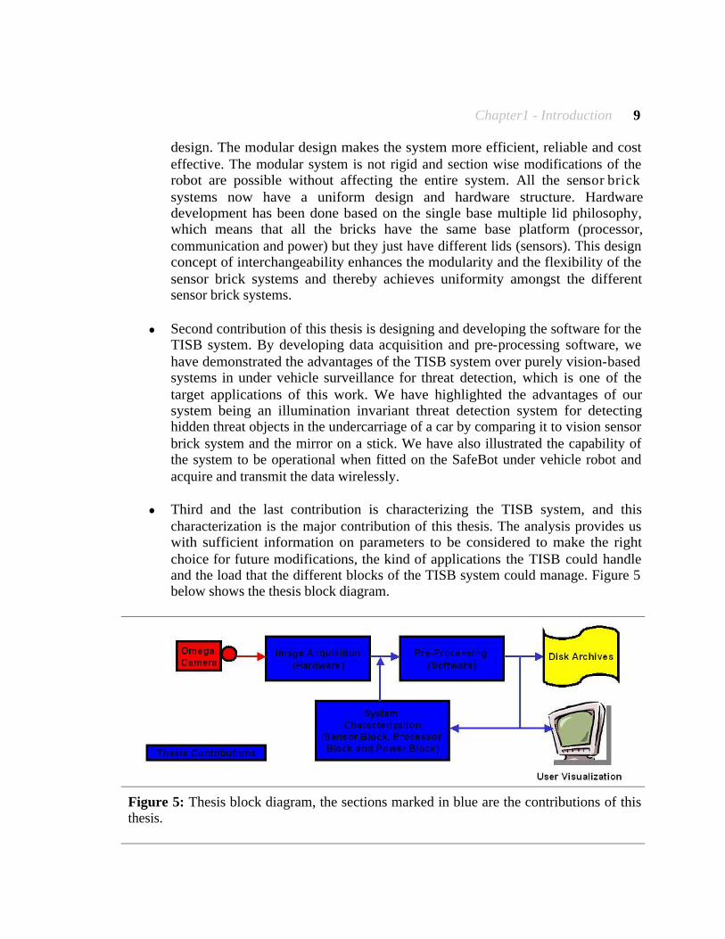
characterization is the major contribution of this thesis. The analysis provides us with sufficient information on parameters to be considered to make the right choice for future modifications, the kind of applications the TISB could handle and the load that the different blocks of the TISB system could manage. Figure 5 below shows the thesis block diagram.
Figure 5: Thesis block diagram, the sections marked in blue are the contributions of this thesis.

Chapter1 - Introduction 10
1.5 Document Outline
This document is divided into three major sections. Chapters 1 and 2 make up the first section. Chapter 1 provides a brief introduction to the thesis, stating the motivation, giving an overview of the thesis and presenting our mission and target applications. Chapter 2 provides a literature review by presenting details on the theory of thermal imaging, previous work and state of the art in the field of robotics. The survey examines hardware and software architecture and presents a comparison with existing competing technologies. Chapters 3 and 4 make up the second section. Chapter 3 presents the overall hardware architecture detailing the sensor brick design philosophy, the thermal sensor brick system, the four different sensor bricks and the evolution of the sensor brick design. Chapter 4 talks about the overall software architecture employed for acquisition, processing and interpretation of data. The third section consists of Chapters 5 and 6. Chapter 5 presents the experimental results for the different areas of experimentation, hardware experiments for characterization of the thermal sensor and scenario experiments for under vehicle surveillance scenario application. Finally Chapter 6 presents a summary of work done, conclusions drawn and lessons learned during the process and lists possible areas of future work.
Chapter 2 – Literature Review 11
2 Literature Review
This chapter on Literature Review has three sub-sections: Theory of Thermal Imaging, Previous Work and Competing Technologies. The section on Theory of Thermal Imaging discusses the working principle of thermal imaging and the general applications of thermal imaging. The section on Previous Work deals with the previous work done on under vehicle surveillance systems, under vehicle imaging robotic systems, and other modular robotic systems. Finally the section on Competing Technologies deals with commercially available search and surveillance systems.
2.1 Theory of Thermal Imaging
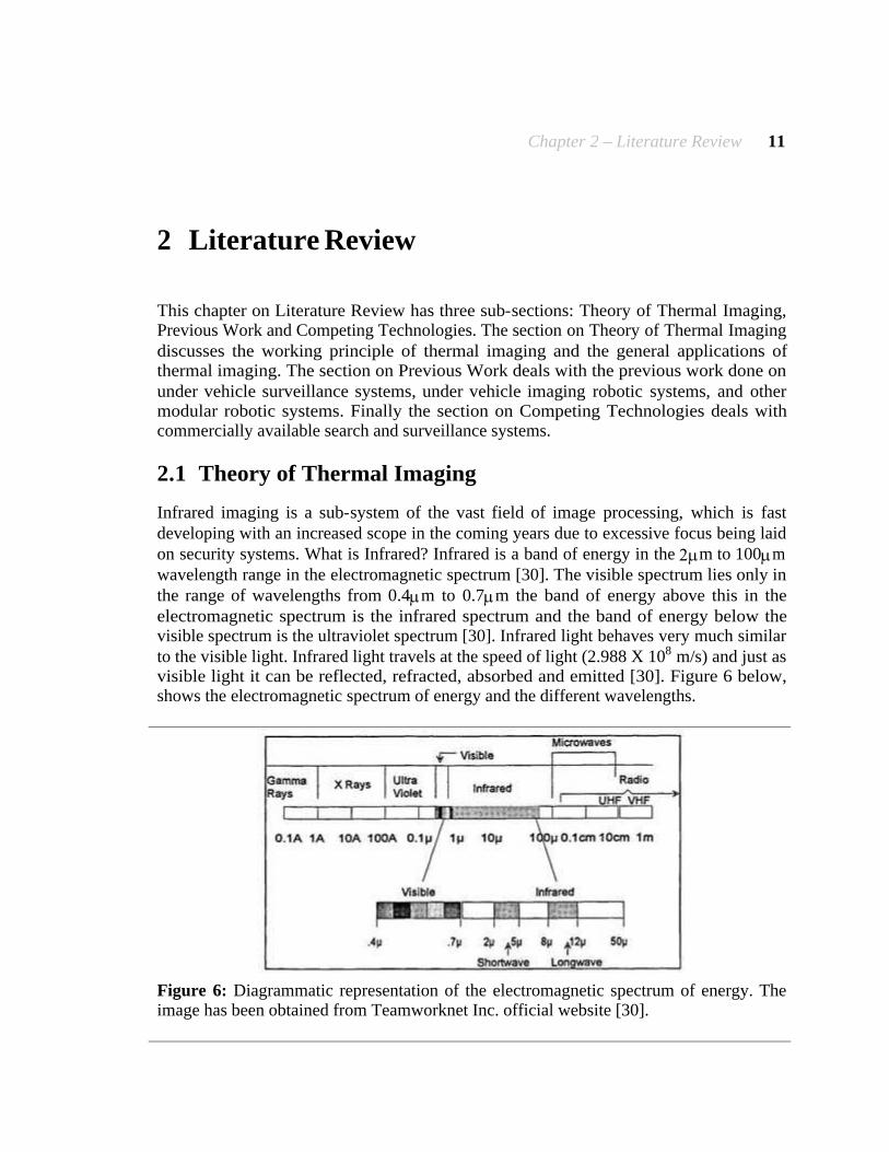
Infrared imaging is a sub-system of the vast field of image processing, which is fast developing with an increased scope in the coming years due to excessive focus being laid on security systems. What is Infrared? Infrared is a band of energy in the 2mm to 100mm wavelength range in the electromagnetic spectrum [30]. The visible spectrum lies only in the range of wavelengths from 0.4mm to 0.7mm the band of energy above this in the electromagnetic spectrum is the infrared spectrum and the band of energy below the visible spectrum is the ultraviolet spectrum [30]. Infrared light behaves very much similar to the visible light. Infrared light travels at the speed of light (2.988 X 10⁸ m/s) and just as visible light it can be reflected, refracted, absorbed and emitted [30]. Figure 6 below, shows the electromagnetic spectrum of energy and the different wavelengths.
Figure 6: Diagrammatic representation of the electromagnetic spectrum of energy. The image has been obtained from Teamworknet Inc. official website [30].

Chapter 2 – Literature Review 12
An infrared image is a pattern generated proportional to a temperature function corresponding to the area or the object that is being imaged. An infrared image is obtained based on the principle that vibration and rotation of atoms and molecules in an object causes the object to give out heat which is captured by an infrared sensor to give us an image [30]. The Stefan-Boltzmann’s law as shown in Equation (1) below, shows us that infrared power of an object is directly proportional to the 4th power of the absolute temperature of the object; hence we can infer from this that the output power of the object would tend to increase very fast with increase in absolute temperature of the object [30].
4Tw s= (1)
Here w = watts/meter2, σ = Stefan-Boltzmann’s Constant (5.6697x10⁻⁶ watts/m2-T), and T = Absolute Temperature Kelvin. The infrared imaging spectrum can be broadly divided into two ranges of wavelengths, the mid wavelength band infrared (MWIR) has an energy spectrum in the 3mm to 5mm range and the long wavelength band infrared (LWIR) has an energy spectrum in the range 8mm to 14mm [30]. The selection of the infrared band depends on the type of performance that is desired for the specific application that it is being used for. Table 1 below lists the applications and advantages of MWIR and LWIR. In Figure 6 above we can see a high interference zone between the two infrared energy band spectrums. It has been observed that MWIR is better suited for hotter objects or in cases where sensitivity is of less importance in relation to contrast [30]. MWIR has an advantage that it requires smaller optics. Traditionally LWIR is preferred in cases where we require high performance infrared imaging since it has a higher sensitivity to ambient temperature of objects and also displays better transmission through smoke, mist and fog. MWIR and LWIR have major differences with regards to background flux, temperature contrasts and atmospheric transmission [30]. Table 1: Applications and advantages of MWIR and LWIR [30].
Mid wavelength band infrared (MWIR) Long wavelength band infrared (LWIR)
· Higher resolution due to a smaller optical diffraction.
· Higher contrast.
· Good only in clear weather conditions.
· Transmission is possible in high humidity conditions.
· Shows a good performance in foggy, hazy and in misty conditions.
· Its transmission is least affected by atmospheric conditions.
· Reduces solar glint and fire glare sensitivity.
Chapter 2 – Literature Review 13
Infrared images are usually used to see those things, which are not naturally visible to the human eyes (i.e. things, which are invisible to normal vision). For instance a thermal image can be used to procure night vision capabilities where by we can detect objects in the dark, which would remain invisible in a normal visual image. Night vision capabilities have useful applications in search and security operations. Infrared images are usually used to see those things, which are not naturally visible to the human eyes (i.e. things, which are invisible to normal vision). For instance a thermal image can be used to procure night vision capabilities where by we can detect objects in the dark, which would remain invisible in a normal visual image. Night vision capabilities have useful applications in search and security operations. A thermal image could also be used to detect visibly opaque items, (i.e.) objects, which are usually hidden behind other objects or things. This task is accomplished by a thermal image which gives us a pattern showing the heat energy emitted in an area or by an object and incase there is any temperature difference in that area or in that object then it will show up very clearly in the image. Thermal images could also be used for face recognition and pattern recognition. In face recognition techniques they could be used as identification markers, which would help in allowing entry and exit to people in secure locations. Another major application of thermal imagery is in quality control systems used in the manufacturing processes of many products ranging from food, glass, cast iron patterns, moulds and others. Here quality assurance and surveillance on the production line could be ensured using thermal imagery. Lets us now get a brief overview on the field of infrared imaging and then take a look at the general applications of infrared imaging.
2.1.1 Overview
Sir John Herchel developed thermal imaging as it stands today in the early 1800’s. He was actually interested in photography and started recording energy in the infrared spectrum by conducting a number of experiments using carbon and alcohol [30]. It has been believed that analysis of humans based on the difference in temperatures in different regions has been long established. The ancient Greeks and before them the Egyptians, knew a method of diagnosing diseases by locating the excessively hot and cold regions in the body [30]. According to the paper in [30] infrared imaging finds applications in three major areas. Infrared imaging is used for monitoring purposes, for research and development purposes and general industrial applications. Firstly monitoring is used for security purposes like monitoring a prison area to maintain a check on the prisoners at night in the dark, to guard a secure location from intruders, in coastal surveillance to look out for enemy vessels during the night in the dark. Also monitoring could be used to look out for possible illegal activities or wrong doings and can be used to protect people from the threat of possible predators in the dark [30]. Secondly monitoring is used to control traffic may it be vehicular traffic or air traffic. Vehicular traffic can be monitored at night using infrared imagery. Air traffic can be monitored in the dark for takeoff and landing in the absence of light. Thirdly monitoring is used in disaster management and in rescue
Chapter 2 – Literature Review 14
operations where infrared images can help us in locating victims, spotting fire and in monitoring rescue and other operations through smoke and fog. Lastly monitoring also finds application in obtaining disaster footages for television and media persons [30]. The applications of infrared imaging for research and development purposes are very varied and include areas like remote sensing, ecology and medical treatment, thermal sensing and thermal design [30]. In remote sensing infrared is used to conduct aerial observation of ocean and land surfaces on earth, observation of volcanic activity, prospecting for mining and other natural reserves and other exploratory operations which may even include military and civilian spying. The application of infrared in ecology and medical treatment is in detecting diseases in plants and animals. Thermal imagery can also help in early detection of diseases like breast cancer and conducting a check up of the eye. They are also used in diagnosing heart diseases and in checking for the functioning of blood streams and the circulatory system. Infrared also finds application in veterinary medicine for diagnosing animals like cats, dogs, horses, etc. In thermal analysis the applications are in design of heat engines, analyzing the thermal insulating capacity or the heat conducting capacity of a body or a substance. In thermal design the applications are in analyzing the heat emission levels and rates, it can also help in evaluating transient thermal phenomenon in electronic components and on a bigger scale in evaluating power plants [30]. The general industrial applications of infrared are in facility monitoring, non-destructive inspections and in managing manufacturing processes [30]. In monitoring facilities like a chemical plant or a nuclear reactor the infrared renders help in looking for abnormal heat emission levels in boilers or distillers. Detection and tracking of gas leakages and faulty piping can also be done. Power transmission line and transformers are also monitored. Infrared finds application in non-destructive testing in situations like inspecting buildings, roofs, walls and floor surfaces. Thermal imagery is also used to inspect cold storage facilities, inspect internal defects in walls and other optically opaque objects [30]. The major industrial application of non-destructive testing is in checking motors, bearings and rings. Managing manufacturing processes accurately is a difficult task and they pose a strong challenge, but the advantages of infrared can be aptly utilized like in the case of maintaining the distribution of heat in a furnace, or in the case of metal rolling processes. Infrared is also used to manage smoke and thermal exhausts and to control the temperature of metallic molding processes [30].
2.1.2 General Applications
The major application of infrared imaging is in giving us night vision capability (i.e. to see people and objects in the dark in the absence of light by creating a pattern in response to the heat radiated by the objects in that area). Thermal images help in sensing and thereby detecting hidden objects or people, which are not naturally visible to the human eye in the dark. This finds major use in both military and civilian search and surveillance applications. Face recognition and Pattern recognition are amongst the more classical
Chapter 2 – Literature Review 15
applications of infrared imaging. This is because thermal images are both pose and illumination invariant and so the prevalent lighting and other conditions that affect visual images do not affect infrared images. The growth of the infrared technology has been a big boon for the maintenance industry since infrared videos help in seeing through visually opaque objects thereby helping in providing vital details for the purpose of predictive maintenance. Over the years the maintenance industry has changed in its approach. Traditionally maintenance was seen necessary only in case of breakdowns, post World War II it became maintenance for the purpose of preventing a breakdown and nowadays it is predictive maintenance [30]. Predictive maintenance takes place in thermal imaging surveys, in electromagnetic testing, breaker relay testing, visual testing and leak testing [30]. Other areas include magnetic particle inspection, ultrasonic inspection, in vibration analysis, in eddy current analysis, also in transformer oil analysis and in X- ray and gamma ray radiography [30]. The ability of infrared images to help detect hot spots and temperature differences without making any physical contact is what makes them special in the process of predictive maintenance [30]. All the possible major applications of infrared imaging as given in the paper in [30] are mentioned below. Infrared imaging is used to inspect heater tubes, in steam / air de-coking, to confirm the readings of a thermocouple, in flame impingement, in refractory breakdown, in condenser fins and to verify spheroid levels [30]. Infrared imaging is also used to check air- leakage in a furnace, locate gas emission; they also find application in the aerospace industry [30]. In electrical systems thermal images are used to inspect power generators and power substations, to evaluate transformers and capacitors [30]. To inspect both rural and urban overhead distribution electrical lines, to inspect electric motors and to check motor control centers, starters, breakers, fuses, cables and wires [30]. The automotive applications of thermal imaging are for detecting faulty fuel injection nozzles, to test the brakes and other engine systems and to evaluate them for performance and cooling efficiencies [30]. Lastly it also finds application in diagnostics for motor racing suspension and tire contacts [30]. In electronic equipments it is used in the process of evaluating and troubleshooting printed circuit boards, in thermal mapping of semiconductor device services and in the evaluation procedure for circuit board components [30]. It is also used to inspect hybrid microcircuits and solder joints, and in the inspection of bonded structures [30]. Like in the case of other fields thermal imaging also has applications in mechanical systems. Here it is used to inspect boilers and kilns, to check building diagnostics and heat loss, and to inspect roofing systems [30]. They are also used to inspect burners for flame impingement and burner management, to analyze the fuel combustion patterns, and to detect thermal patterns on boiler tubes and measures the tube skin temperature during the normal or standby operation [30]. It is used to scan and record temperatures in the unmonitored areas of the boiler, to scan the exterior of the boiler for refectory damage or

Chapter 2 – Literature Review 16
to locate warmer areas [30]. Infrared images also help in detecting coke buildup in crude furnaces, flue gas leaks in power plant boilers [30]. They are used to inspect mechanical bearings, evaluate heating, ventilation and air conditioning equipment, evaluate cold storage for cooling losses and lastly check refrigeration equipment for insulation leaks. In the field of medical science and veterinary medicine infrared imaging is used to look for diseases like breast cancer and arthritis, to conduct medical examinations for whiplash, back injuries and carpal tunnel syndrome [30]. It is also used in dentistry and to evaluate sports injuries and to monitor the recovery processes [30]. In veterinary medicine it is used to check for injuries, stress fractures and lameness [30]. Thermal imaging helps us in detecting sensations like pain, numbness, etc; which would not have been seen by a normal image because these are problems in the functions of the tissues and not with the structures [31]. Infrared imaging helps us in detecting alterations of the body’s workings like pain and inflammation, nerve irritation and dysfunction, angiogenesis (new blood vessel formation), circulatory incompetencies and treatment efficacies. All these cannot be detected by regular imaging [31]. Infrared imaging is used for assessing pain and inflammation. In this it helps in assessing musculo-skeletal and articular pain, in assessing the efficacy of chiropractic, osteopathic, physiotherapy, acupuncture and myotherpy care [31]. It is used in assessing post injury trauma, in post surgery assessment and in confirming the diagnosis of certain diseases [31]. The next application is in assessing nerve dysfunction and irritation. In this it helps us in examining and correlating between the musculo skeletal finding and neurological irritations or impairment and also in looking at suspected nerve entrapments [31]. It is used to assess for reflex sympathetic dystrophy, complex regional pain disorder, sympathectomies and nerve blocks [31]. In the case of investigating for angiogenesis infrared imagery helps in breast imaging along with anatomical screening, also helps in post skin cancer investigations and in assessing the level of acceptance or rejection after a skin graft [31]. Lastly in the case of circulatory insufficiencies infrared helps in mapping the varicose vein [31]. Many countries used infrared imagers to guard against the entry of the SARS virus to detect passengers with a high body temperature entering their country. Infrared imaging is proving to be a very useful tool in the hands of the law enforcement professionals by helping them in stopping crime before it happens [32]. Since a thermal imager is capable of measuring very small temperature differences it allows us to see in almost zero lighting conditions by taking these images and creating an infrared picture. Law enforcement authorities can use these pictures to catch criminals. This ability of the thermal imager to help in preventing crime is recognized by an association called the Law Enforcement Thermographers Association (LETA) and they have 12 accepted applications of thermal imaging, which can help in crime prevention. These applications are accepted after any judgment passed by the state or federal court accepts infrared images as evidence in a case and are mentioned below [32].

Chapter 2 – Literature Review 17
· Hidden compartments: thermal imaging can help in detecting hidden compartments in vehicles, which may be used for transporting illegal drugs, contraband or even people. Since a thermal imager can detect any change in the thermal characteristics of a surface caused by an adjoining wall or bulkhead it will highlight these structural details invisible to the naked eye [32].
· Perimeter Surveillance: an infrared imager can help in the day and night monitoring of highly restricted facilities and thereby help in spotting and apprehending suspects who may be invading that secure area [32].
· Marine and Ground Surveillance: the night vision capabilities of a thermal imager help in tracking during the night for both navigational as well as surveillance purposes [32].
· Structure Profiles: the structure profile of a building obtained by using an infrared imager will show the heat radiated by the building, and any unexpected excessive radiation can help in checking for unwanted activities [32].
· Officer Safety: during night patrolling the officers can use infrared imagers to look out for hidden suspects, guard dogs and other dangerous obstacles, which are not visible to the human eye in the dark. Also they can do all this without being exposed in the open. They can also use this to see through smoke and dust [32].
· Disturbed surface scenarios: a surface may it be the earth surface or any other artificial surface even though it is not apparently visibly disturbed will radiate heat differently and so an infrared imager will help us in looking for hidden compartments or floors [32].
· Environmental: air, water or soil pollutants radiate heat differently then their surroundings and this difference in heat can be easily detected using an infrared imager and the pollutants can be tracked back to their source [32].
· Flight safety: infrared imagers give night time vision to aircrafts thereby helping them in detecting power lines and unlit landing sights and other such obstacles in their pathway [32].
· Fugitive searches and rescue missions: living objects such as human beings and animals are excellent radiators of heat hence infrared imaging can be used in search and rescue operations to look for people who may be invisible to normal vision due to optical shielding. The radiated heat is easily detected and the suspect can be spotted from his hideout [32].
· Vehicle pursuits: vehicles radiate a lot of heat both while in use and even after sometime. This heat shows up not only from the engine but also from the tires, brakes and the exhaust. Using a thermal imager the police can spot a vehicle, which may even, be driving with its headlights turned off to avoid being spotted. Also a suspects car, which has just entered a parking lot, can be detected from it heat emission [32].
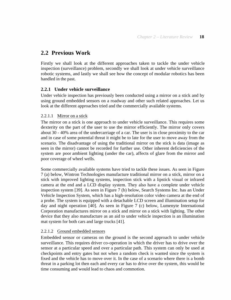
Chapter 2 – Literature Review 18
2.2 Previous Work
Firstly we shall look at the different approaches taken to tackle the under vehicle inspection (surveillance) problem, secondly we shall look at under vehicle surveillance robotic systems, and lastly we shall see how the concept of modular robotics has been handled in the past.
2.2.1 Under vehicle surveillance Under vehicle inspection has previously been conducted using a mirror on a stick and by using ground embedded sensors on a roadway and other such related approaches. Let us look at the different approaches tried and the commercially available systems.
2.2.1.1 Mirror on a stick
The mirror on a stick is one approach to under vehicle surveillance. This requires some dexterity on the part of the user to use the mirror efficiently. The mirror only covers about 30 - 40% area of the undercarriage of a car. The user is in close proximity to the car and in case of some potential threat it might be to late for the user to move away from the scenario. The disadvantage of using the traditional mirror on the stick is data (image as seen in the mirror) cannot be recorded for further use. Other inherent deficiencies of the system are poor ambient lighting (under the car), affects of glare from the mirror and poor coverage of wheel wells. Some commercially available systems have tried to tackle these issues. As seen in Figure 7 (a) below, Wintron Technologies manufacture traditional mirror on a stick, mirror on a stick with improved lighting systems, inspection stick with a lipstick visual or infrared camera at the end and a LCD display system. They also have a complete under vehicle inspection system [39]. As seen in Figure 7 (b) below, Search Systems Inc. has an Under Vehicle Inspection System, which has a high-resolution color video camera at the end of a probe. The system is equipped with a detachable LCD screen and illumination setup for day and night operation [40]. As seen in Figure 7 (c) below, Lumenyte International Corporation manufactures mirror on a stick and mirror on a stick with lighting. The other device that they also manufacture as an aid to under vehicle inspection is an illumination mat system for both cars and large trucks [41].
2.2.1.2 Ground embedded sensors
Embedded sensor or cameras on the ground is the second approach to under vehicle surveillance. This requires driver co-operation in which the driver has to drive over the sensor at a particular speed and over a particular path. This system can only be used at checkpoints and entry gates but not when a random check is wanted since the system is fixed and the vehicle has to move over it. In the case of a scenario where there is a bomb threat in a parking lot then each and every car has to drive over the system, this would be time consuming and would lead to chaos and commotion.

Chapter 2 – Literature Review 19
(a) Under vehicle inspection systems by Wintron Technologies [39].
(b) Under vehicle inspection systems by Search Systems Inc [40].
(c) Under vehicle inspection systems by Lumenyte International Corporation [41].
Figure 7: Different currently commercially available mirror on a stick type under vehicle surveillance systems.
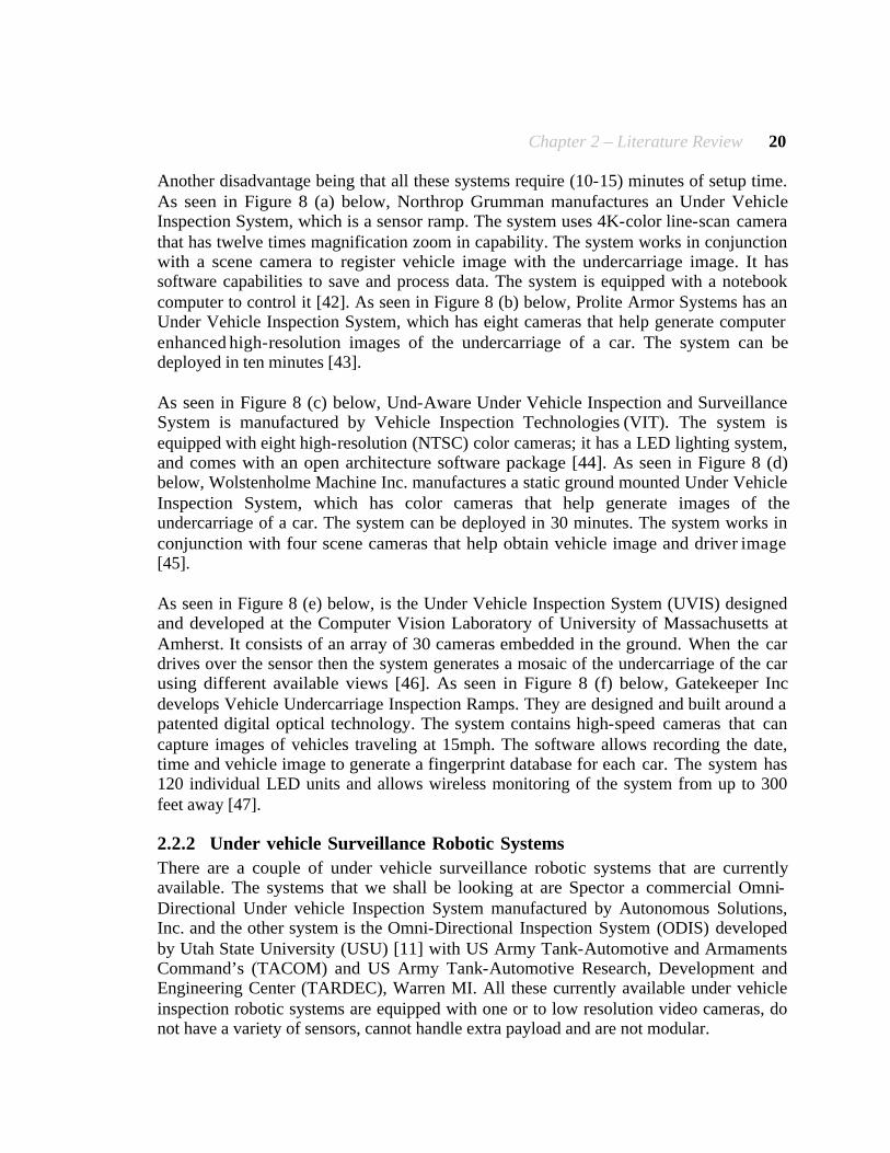
Chapter 2 – Literature Review 20
Another disadvantage being that all these systems require (10-15) minutes of setup time. As seen in Figure 8 (a) below, Northrop Grumman manufactures an Under Vehicle Inspection System, which is a sensor ramp. The system uses 4K-color line-scan camera that has twelve times magnification zoom in capability. The system works in conjunction with a scene camera to register vehicle image with the undercarriage image. It has software capabilities to save and process data. The system is equipped with a notebook computer to control it [42]. As seen in Figure 8 (b) below, Prolite Armor Systems has an Under Vehicle Inspection System, which has eight cameras that help generate computer enhanced high-resolution images of the undercarriage of a car. The system can be deployed in ten minutes [43]. As seen in Figure 8 (c) below, Und-Aware Under Vehicle Inspection and Surveillance System is manufactured by Vehicle Inspection Technologies (VIT). The system is equipped with eight high-resolution (NTSC) color cameras; it has a LED lighting system, and comes with an open architecture software package [44]. As seen in Figure 8 (d) below, Wolstenholme Machine Inc. manufactures a static ground mounted Under Vehicle Inspection System, which has color cameras that help generate images of the undercarriage of a car. The system can be deployed in 30 minutes. The system works in conjunction with four scene cameras that help obtain vehicle image and driver image [45]. As seen in Figure 8 (e) below, is the Under Vehicle Inspection System (UVIS) designed and developed at the Computer Vision Laboratory of University of Massachusetts at Amherst. It consists of an array of 30 cameras embedded in the ground. When the car drives over the sensor then the system generates a mosaic of the undercarriage of the car using different available views [46]. As seen in Figure 8 (f) below, Gatekeeper Inc develops Vehicle Undercarriage Inspection Ramps. They are designed and built around a patented digital optical technology. The system contains high-speed cameras that can capture images of vehicles traveling at 15mph. The software allows recording the date, time and vehicle image to generate a fingerprint database for each car. The system has 120 individual LED units and allows wireless monitoring of the system from up to 300 feet away [47].
2.2.2 Under vehicle Surveillance Robotic Systems
There are a couple of under vehicle surveillance robotic systems that are currently available. The systems that we shall be looking at are Spector a commercial Omni-Directional Under vehicle Inspection System manufactured by Autonomous Solutions, Inc. and the other system is the Omni-Directional Inspection System (ODIS) developed by Utah State University (USU) [11] with US Army Tank-Automotive and Armaments Command’s (TACOM) and US Army Tank-Automotive Research, Development and Engineering Center (TARDEC), Warren MI. All these currently available under vehicle inspection robotic systems are equipped with one or to low resolution video cameras, do not have a variety of sensors, cannot handle extra payload and are not modular.

Chapter 2 – Literature Review 21
(a) Under vehicle inspection system by
Northrop Grumman [42]. (b) Under vehicle inspection system by
Prolite Armor Systems [43].
(c) Under vehicle inspection system by Vehicle Inspection Technologies [44].
(d) Under vehicle inspection system by Wolstenholme Machine Inc. [45].
(e) Under vehicle inspection system by University of Massachusetts Amherst [46].
(f) Under vehicle inspection system by Gatekeeper Inc. [47].
Figure 8: Different currently commercially available ground embedded sensors under vehicle surveillance systems.
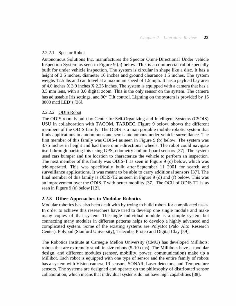
Chapter 2 – Literature Review 22
2.2.2.1 Spector Robot
Autonomous Solutions Inc. manufactures the Spector Omni-Directional Under vehicle Inspection System as seen in Figure 9 (a) below. This is a commercial robot specially built for under vehicle inspection. The system is circular in shape like a disc. It has a height of 3.5 inches, diameter 16 inches and ground clearance 1.5 inches. The system weighs 12.5 lbs and can travel at a maximum speed of 1.5 mph. It has a payload bay area of 4.0 inches X 3.9 inches X 2.25 inches. The system is equipped with a camera that has a 3.5 mm lens, with a 3.0 digital zoom. This is the only sensor on the system. The camera has adjustable Iris settings, and 90° Tilt control. Lighting on the system is provided by 15 8000 mcd LED’s [36].
2.2.2.2 ODIS Robot
The ODIS robot is built by Center for Self-Organizing and Intelligent Systems (CSOIS) USU in collaboration with TACOM, TARDEC. Figure 9 below, shows the different members of the ODIS family. The ODIS is a man portable mobile robotic system that finds applications in autonomous and semi-autonomous under vehicle surveillance. The first member of this family was ODIS-I as seen in Figure 9 (b) below. The system was 3.75 inches in height and had three omni-directional wheels. The robot could navigate itself through parking lots using GPS, odometry and on-board sensors [37]. The system used cars bumper and tire location to characterize the vehicle to perform an inspection. The next member of this family was ODIS-T as seen in Figure 9 (c) below, which was tele-operated. This was specifically built after September 11 2001 for search and surveillance applications. It was meant to be able to carry additional sensors [37]. The final member of this family is ODIS-T2 as seen in Figure 9 (d) and (f) below. This was an improvement over the ODIS-T with better mobility [37]. The OCU of ODIS-T2 is as seen in Figure 9 (e) below [12].
2.2.3 Other Approaches to Modular Robotics Modular robotics has also been dealt with by trying to build robots for complicated tasks. In order to achieve this researchers have tried to develop one single module and make many copies of that system. The single individual module is a simple system but connecting many modules in different patterns helps to develop a highly advanced and complicated system. Some of the existing systems are PolyBot (Palo Alto Research Center), Polypod (Stanford University), Telecube, Proteo and Digital Clay [59]. The Robotics Institute at Carnegie Mellon University (CMU) has developed Millibots; robots that are extremely small in size robots (5-10 cms). The Millibots have a modular design, and different modules (sensor, mobility, power, communication) make up a Millibot. Each robot is equipped with one type of sensor and the entire family of robots has a system with Vision camera, IR sensors, SONAR, Laser detectors, and Temperature sensors. The systems are designed and operate on the philosophy of distributed sensor collaboration, which means that individual systems do not have high capabilities [38].

Chapter 2 – Literature Review 23
(a) Spector Omni-Directional Under vehicle Inspection System by Autonomous Solutions Inc. [36].
(b) ODIS-I [37] (c) ODIS-T [37] (d) ODIS-T2 in operation in
Iraq [12]
(e) ODIS-T2 OCU [12]. (f) ODIS-T2 and the image seen by it [37].
Figure 9: Different currently available under vehicle surveillance robotics systems.
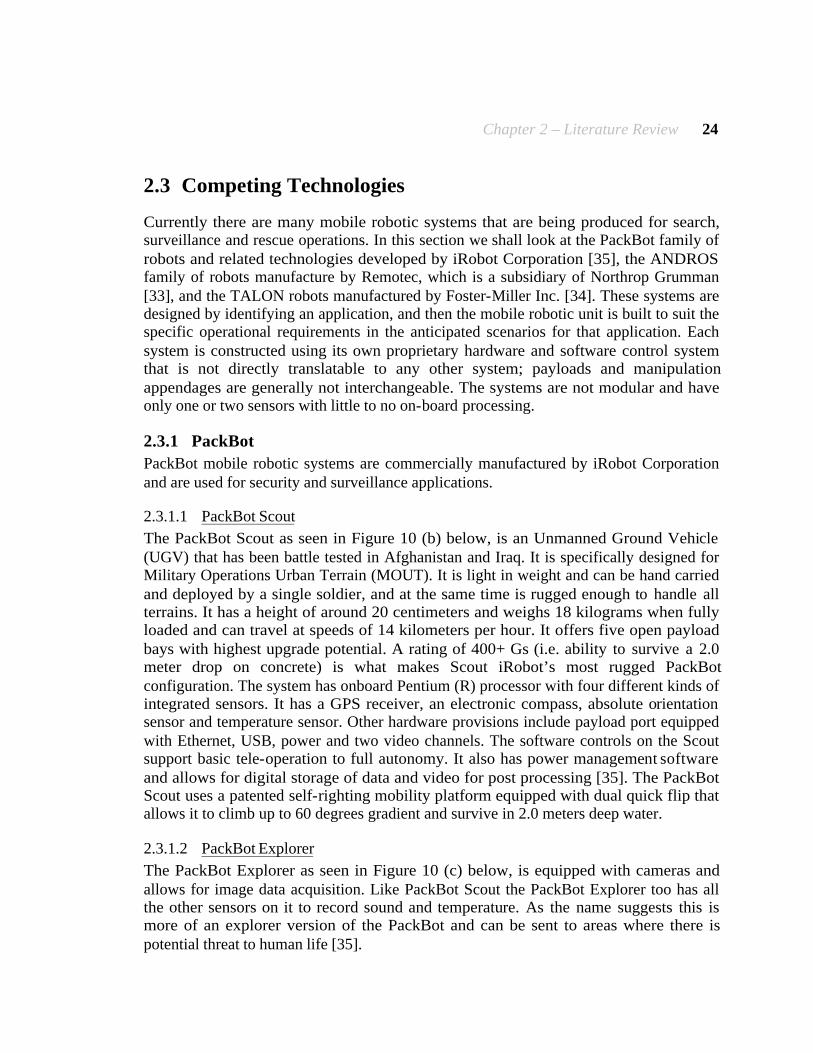
Chapter 2 – Literature Review 24
2.3 Competing Technologies
Currently there are many mobile robotic systems that are being produced for search, surveillance and rescue operations. In this section we shall look at the PackBot family of robots and related technologies developed by iRobot Corporation [35], the ANDROS family of robots manufacture by Remotec, which is a subsidiary of Northrop Grumman [33], and the TALON robots manufactured by Foster-Miller Inc. [34]. These systems are designed by identifying an application, and then the mobile robotic unit is built to suit the specific operational requirements in the anticipated scenarios for that application. Each system is constructed using its own proprietary hardware and software control system that is not directly translatable to any other system; payloads and manipulation appendages are generally not interchangeable. The systems are not modular and have only one or two sensors with little to no on-board processing.
2.3.1 PackBot
PackBot mobile robotic systems are commercially manufactured by iRobot Corporation and are used for security and surveillance applications.
2.3.1.1 PackBot Scout
The PackBot Scout as seen in Figure 10 (b) below, is an Unmanned Ground Vehicle (UGV) that has been battle tested in Afghanistan and Iraq. It is specifically designed for Military Operations Urban Terrain (MOUT). It is light in weight and can be hand carried and deployed by a single soldier, and at the same time is rugged enough to handle all terrains. It has a height of around 20 centimeters and weighs 18 kilograms when fully loaded and can travel at speeds of 14 kilometers per hour. It offers five open payload bays with highest upgrade potential. A rating of 400+ Gs (i.e. ability to survive a 2.0 meter drop on concrete) is what makes Scout iRobot’s most rugged PackBot configuration. The system has onboard Pentium (R) processor with four different kinds of integrated sensors. It has a GPS receiver, an electronic compass, absolute orientation sensor and temperature sensor. Other hardware provisions include payload port equipped with Ethernet, USB, power and two video channels. The software controls on the Scout support basic tele-operation to full autonomy. It also has power management software and allows for digital storage of data and video for post processing [35]. The PackBot Scout uses a patented self-righting mobility platform equipped with dual quick flip that allows it to climb up to 60 degrees gradient and survive in 2.0 meters deep water.
2.3.1.2 PackBot Explorer
The PackBot Explorer as seen in Figure 10 (c) below, is equipped with cameras and allows for image data acquisition. Like PackBot Scout the PackBot Explorer too has all the other sensors on it to record sound and temperature. As the name suggests this is more of an explorer version of the PackBot and can be sent to areas where there is potential threat to human life [35].

Chapter 2 – Literature Review 25
(a) Soldier carrying a PackBot [35]. (b) iRobot PackBot Scout [35].
(c) iRobot PackBot Explorer [35]. (d) iRobot PackBot EOD. [35].
Figure 10: Different members of the PackBot family of robots manufactured by iRobot Corporation [35].

Chapter 2 – Literature Review 26
2.3.1.3 PackBot EOD
The PackBot EOD as seen in Figure 10 (d) above, is a rugged lightweight robot specifically designed to aid in Explosive Ordnance Disposal (EOD), HAZMAT, search and surveillance, rescue operations, bomb squad operations, SWAT teams and military operations. Equipped with a lightweight rugged Omni Reach Manipulator system that can stretch out 2.0 meters in any direction the PackBot EOD is designed for IED and EOD disposal. A single soldier can easily deploy a fully loaded PackBot EOD that weighs 24 kilograms. It can traverse narrow and difficult terrain at speeds of up to 5.5 kilometers per hour. Like the PackBot Explorer the PackBot EOD too has tracked QuickFlip(TM) dual rotating flippers that allows easy maneuverability. The low-profile gripper on the robot allows it to perform multiple manipulation tasks. The system is equipped to carry, video/audio, chemical-bio sensors, mine detectors, ground-penetrating radar (GPR) and extra power payloads [35].
2.3.1.4 R-Gator: Autonomous Unmanned Ground Vehicle
The R-Gator as seen in Figure 11 (a) below, is a system developed by incorporating iRobot robotic controls on a John Deere M-GatorTM and has applications like unmanned scout, perimeter guard, pack/ammo/supply carrier and other applications for soldiers, airmen and marines. Some of the features available on the R-Gator are tele-operation, manual operation, autonomous waypoint navigation, obstacle avoidance and robotic following [35].
2.3.1.5 Research and Development at iRobot
Some of the systems in development at the iRobot Corporation are Wayfarer, Future Combat Systems (FCS) and NEOMover [35]. Wayfarer the fully autonomous urban reconnaissance PackBot is developed by iRobot on a project by TACOM TARDEC. Its target applications are Route Reconnaissance (i.e. moving ahead of a soldier and leading the way with maps and video of what lies ahead), Perimeter Reconnaissance (i.e. traversing the perimeter of a building and returning maps and video), and Street-Based Reconnaissance (i.e. moving down city roads using GPS/INS and collecting maps and video of urban terrain). The modular wayfarer navigation payload can connect with standard PackBot payload like LIDAR, stereovision, FLIR and INS sensors [35]. The iRobot’s FCS system as seen in Figure 11 (b) below, that is being developed is a next generation Small Unmanned Ground Vehicle (SUGV) and will be capable of efficiently performing tasks inaccessible or too dangerous for humans. The 30-pound SUGV is an evolution of the 48-pound PackBot Explorer and will have integrated sensors [35]. NEOMover as seen in Figure 11 (b) below is a 200-pound New Explosive Ordnance Mover that is a tracked vehicle with small footprint and high mobility. It has some provisions for incorporating modular payloads [35].
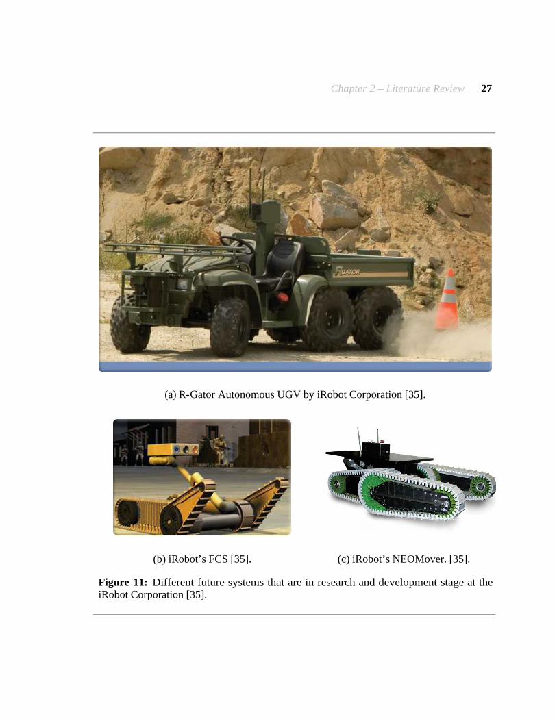
Chapter 2 – Literature Review 27
(a) R-Gator Autonomous UGV by iRobot Corporation [35].
(b) iRobot’s FCS [35]. (c) iRobot’s NEOMover. [35].
Figure 11: Different future systems that are in research and development stage at the iRobot Corporation [35].

Chapter 2 – Literature Review 28
2.3.2 ANDROS
ANDROS mobile robotic systems used by many military and police units around the world are commercially manufactured by Remotec Inc a subsidiary of Northrop Grumman.
2.3.2.1 F6A
The ANDROS F6A as seen in Figure 12 (a) below is a versatile heavy-duty robot of the ANDROS series. It has a height of 56.5 inches, width 59 inches, length 52 inches and ground clearance 3.5 inches. It weighs 485 lbs and can travel at speeds of up to 3.5 miles per hour. It is equipped with a color surveillance camera with light, (216:1) zoom, pan/tilt and 24- inch vertical extender. The stationary arm is also equipped with a camera (40:1) zoom. It has mission specific plug and play tool/sensor/weapon mounts. A Manipulators arm with seven degrees of freedom and a gripper with continuous rotate makes the system highly flexible. Mobility on the system is ensured through patented articulated tracking that allows traversing ditches, obstacles and tough terrains. The system also has quick release pneumatic wheels and can handle slopes of up to 45 degrees including stairs. Communication on the system is achieved through fiber-optic cable deployed from the vehicle, radio control (wireless) and hard-tether cable. The system is sealed all weather resistant and can handle wet and dry conditions. The system comes with an Operator Control Unit (OCU), which allows viewing the live video stream and other sensor information. The robot controls are also located on the OCU [33].
2.3.2.2 Mark V-A1
The ANDROS Mark V-A1 as seen in Figure 12 (b) below, is a robot of the ANDROS series used for hazardous operations. It has a height of 46.5 inches, width 43 inches, length 48 inches and ground clearance 5.3 inches. It weighs 790 lbs and can travel at speeds of up to 3.5 miles per hour. It is equipped with a color surveillance camera with light, (216:1) zoom, pan/tilt and 24- inch vertical extender. It has mission specific plug and play tool/sensor/weapon mounts. A Manipulators arm with seven degrees of freedom and a gripper with continuous rotate makes the system highly flexible. Mobility on the system is ensured through patented articulated tracking that allows traversing ditches, obstacles and tough terrains. The system also has quick release pneumatic wheels and can handle slopes of up to 45 degrees including stairs. Communication on the system is achieved through fiber-optic cable deployed from the vehicle, radio control (wireless) and hard-tether cable. The system is sealed all weather resistant and can handle wet and dry conditions. The system comes with an OCU, which allows viewing the live video stream and other sensor information. The robot controls are also located on the OCU [33].
2.3.2.3 Mini-Andros-II
The Mini-ANDROS Mark II as seen in Figure 12 (c) below, is a full- featured entry- level robot of the ANDROS series used for hazardous operations. It has a height of 27 inches, width 24.5 inches, length 53 inches and ground clearance 3.0 inches.
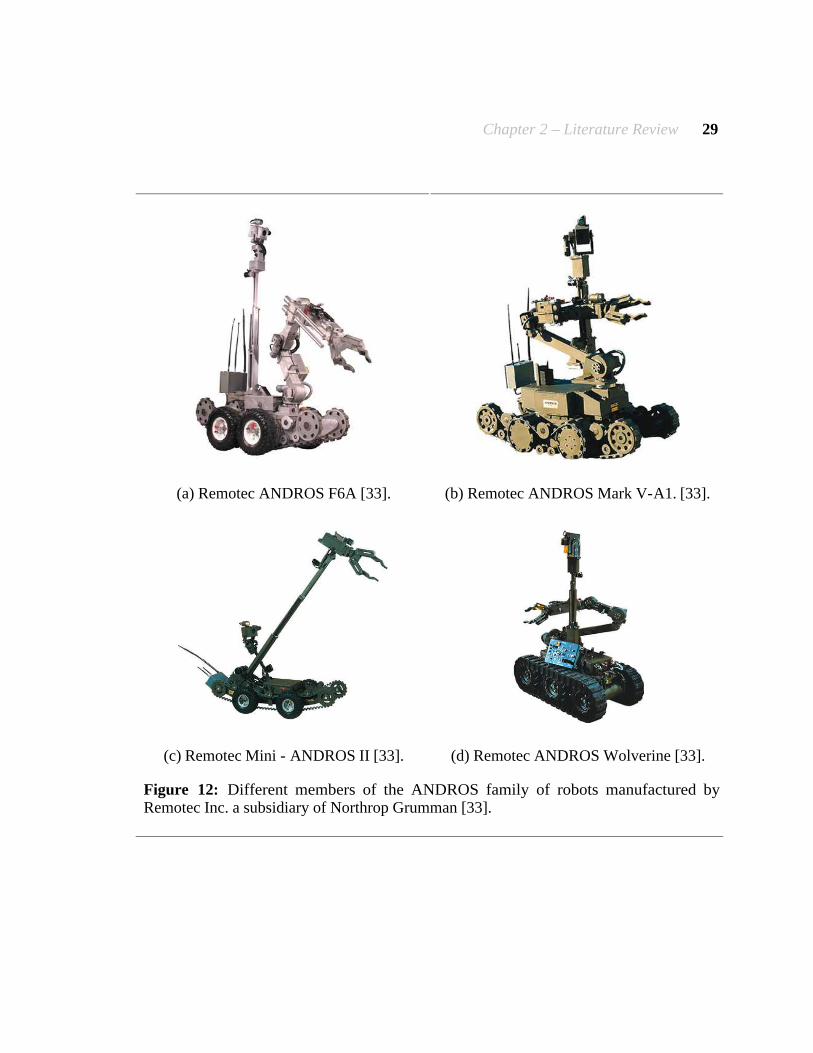
Chapter 2 – Literature Review 29
(a) Remotec ANDROS F6A [33]. (b) Remotec ANDROS Mark V-A1. [33].
(c) Remotec Mini - ANDROS II [33]. (d) Remotec ANDROS Wolverine [33].
Figure 12: Different members of the ANDROS family of robots manufactured by Remotec Inc. a subsidiary of Northrop Grumman [33].

Chapter 2 – Literature Review 30
It weighs 225 lbs and can travel at speeds of up to 1.1 miles per hour. It is equipped with a color surveillance camera (6:1) zoom, pan/tilt and 18- inch fold down extender. Two-meter telescopic arm with four degrees of freedom makes the system flexible. The system employs single module electronics for quick in field replacement. Mobility on the system is ensured through patented articulated tracking that allows traversing ditches, obstacles and tough terrains. The system has quick free wheel option and can handle slopes of up to 45 degrees including stairs. Communication on the system is achieved through fiber-optic cable deployed from the vehicle, radio control (wireless) and hard-tether cable. The system is sealed all weather resistant and can handle wet and dry conditions. The system comes with an OCU, which allows viewing the live video stream and other sensor information. The robot controls are also located on the OCU [33].
2.3.2.4 Wolverine
The ANDROS Wolverine as seen in Figure 12 (d) above, is a workhorse robot of the ANDROS series. It is a heavy-duty extremely strong robot that can handle all terrains with extreme dexterity. It has a height of 69 inches, width 29 inches, length 58 inches and ground clearance 5.5 inches. It weighs 810 lbs and can travel at speeds of up to 2.0 miles per hour. It is equipped with a color surveillance camera with light, (216:1) zoom, pan/tilt and 24- inch vertical extender. Dual accessory mount on the arm allows simultaneous multiple tool/sensor/weapon mounts. The system employs single module electronics for quick in field replacement. A Manipulators arm with seven degrees of freedom and a gripper with continuous rotate makes the system highly flexible. Mobility on the system is ensured through six individually powered wheels with lockout hubs for freewheeling. Optional tracks allow traversing ditches, obstacles and tough terrains. The system can handle slopes of up to 45 degrees including stairs. Communication on the system is achieved through fiber-optic cable deployed from the vehicle, radio control (wireless) and hard-tether cable. The system is sealed all weather resistant and can handle wet and dry conditions. The system comes with an OCU, which allows viewing the live video stream and other sensor information. The robot controls are also located on the OCU [33].
2.3.3 TALON Foster Miller Inc. commercially manufactures TALON mobile robotic systems. The TALON is a powerful, durable lightweight tracked robot used widely for applications such as EOD, reconnaissance, communications, sensing, security, defense and rescue. As seen in Figure 13 below TALON’s are all-weather, day/ night robots with amphibious capabilities and can navigate all kinds of terrain like stairs and rubble. The TALON weighs 100 lbs (45 Kgs) and is man portable and can be deployed instantly. The TALON is available in 80 different application specific configurations. The TALON is available with seven different speed settings and is the fastest commercial robot. It has a high payload capacity (i.e. highest payload to weight ratio) and has longest battery life for any man portable robotic system [34]. The TALON employs wired and wireless communication (less than one mile).
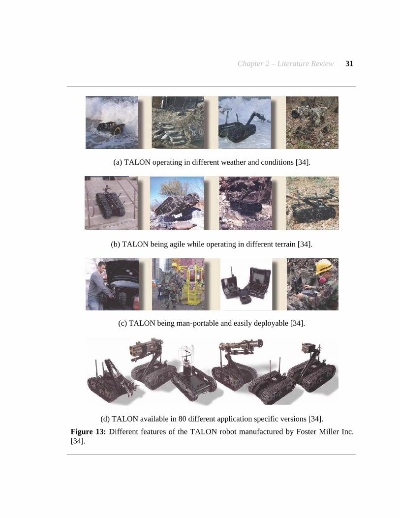
Chapter 2 – Literature Review 31
(a) TALON operating in different weather and conditions [34].
(b) TALON being agile while operating in different terrain [34].
(c) TALON being man-portable and easily deployable [34].
(d) TALON available in 80 different application specific versions [34].
Figure 13: Different features of the TALON robot manufactured by Foster Miller Inc. [34].

Chapter 2 – Literature Review 32
The TALON has a height 11 inches (arm stowed) and 52 inches (arm extended), width 22.5 inches, length 34 inches, horizontal reach 52 inches, and ground clearance 2.75 inches. It weighs 115lbs–140lbs and can travel at speeds of up to 5.2 miles per hour. It is equipped with a color camera (300:1) zoom and three (gripper, elbow, rear) night vision cameras. Up to seven cameras can be attached to the system. The system can handle slopes of up to 43 degrees (stairs) and 40 degrees (slide slope). The system has a Payload Capacity of 100 lbs, Drag Capacity with Gripper of 100lbs and Tow Capacity of 200lbs. The system is sealed all weather resistant and can handle wet and dry conditions. The system comes with an OCU, which allows viewing the live video stream and other sensor information. The robot controls are also located on the OCU [34]. Discussed below are some of the application specific TALON robots, they are shown in Figure 14 below.
2.3.3.1 TALON for EOD/IED Missions
TALON –Engineer robot designed for EOD/IED mission has been used at ground zero on September 11 and is also being used in Iraq and Afghanistan. This system has heavy-duty tracks instead of the regular ones, additional digging tools, night vision cameras with zoom and a microphone to pick up ambient sound [34].
2.3.3.2 TALON for Reconnaissance
A version of the TALON weighing only 60lbs (27 Kgs) and equipped with day/night color cameras, listening devices and all other features of the large TALON except an arm or a gripper is used for reconnaissance operations [34].
2.3.3.3 TALON for Armed Reconnaissance
TALON robots configured with M16, M240 or M249 machine guns, or Barrett 50-caliber rifles, or 40mm grenade launchers and M202 anti-tank launchers are used for armed reconnaissance operations [34].
2.3.3.4 TALON for HAZMAT First Responders
TALON robot equipped with COTS chemical, gas, temperature and radiation sensors is built as First Responder for hazardous materials. The chemical sensor can detect chemical warfare agents, gamma radiation and irritants such as pepper spray and mace. The gas sensor can measure 50 gases including carbon dioxide, methane, propane, fuels and solvents. The thermometer can perform up to 1°C accuracy temperature of fire across a wall. The radiation sensor can record radiological exposure rates from 1.0 micro-Roentgen per hour to 10.0 Roentgen per hour [34]. Using a hand-held PDA we can control all the four sensors.

Chapter 2 – Literature Review 33
(a) Chemical, Gas and Radiation [34]. (b) Individual soldiers version [34].
(c) Small mobile weapons for battle [34].
(c) SWAT teams and HAZMAT operations [34].
Figure 14: Different application specific designs of the TALON family of robots manufactured by Foster Miller Inc. [34].
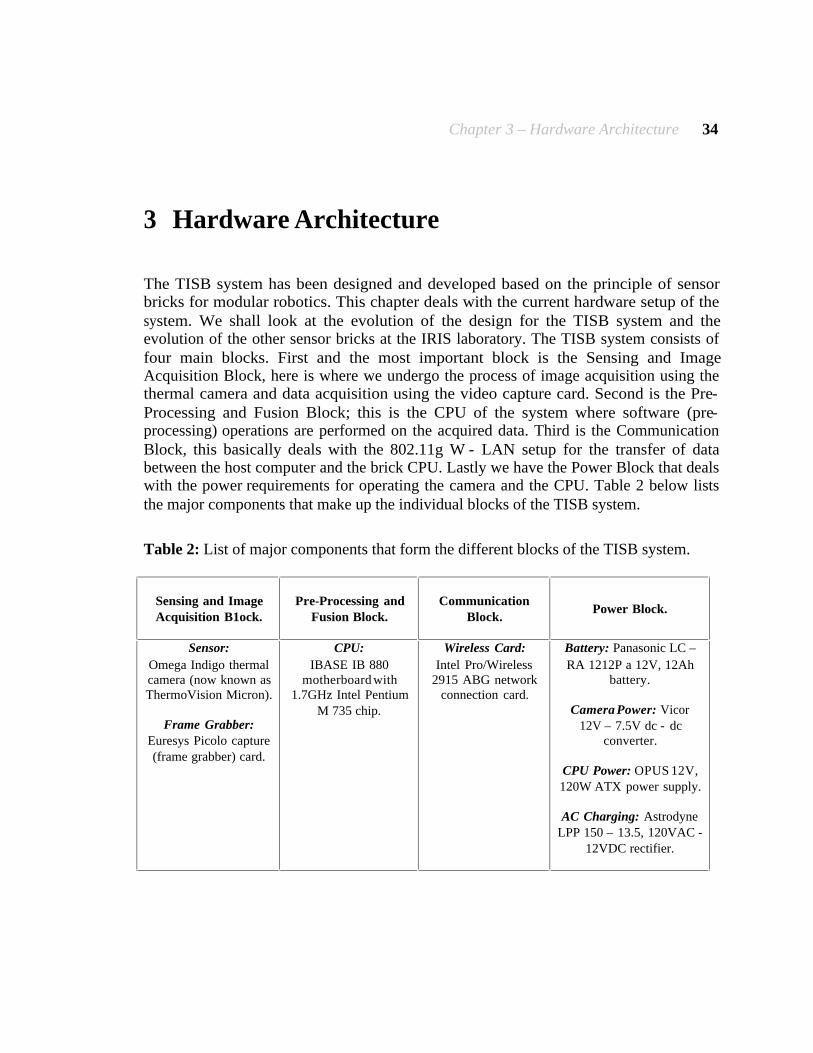
Chapter 3 – Hardware Architecture 34
3 Hardware Architecture
The TISB system has been designed and developed based on the principle of sensor bricks for modular robotics. This chapter deals with the current hardware setup of the system. We shall look at the evolution of the design for the TISB system and the evolution of the other sensor bricks at the IRIS laboratory. The TISB system consists of four main blocks. First and the most important block is the Sensing and Image Acquisition Block, here is where we undergo the process of image acquisition using the thermal camera and data acquisition using the video capture card. Second is the Pre-Processing and Fusion Block; this is the CPU of the system where software (pre-processing) operations are performed on the acquired data. Third is the Communication Block, this basically deals with the 802.11g W - LAN setup for the transfer of data between the host computer and the brick CPU. Lastly we have the Power Block that deals with the power requirements for operating the camera and the CPU. Table 2 below lists the major components that make up the individual blocks of the TISB system.
Table 2: List of major components that form the different blocks of the TISB system.
Sensing and Image Acquisition B1ock.
Pre-Processing and Fusion Block.
Communication Block.
Power Block.
Sensor:
Omega Indigo thermal camera (now known as ThermoVision Micron).
Frame Grabber:
Euresys Picolo capture (frame grabber) card.
CPU:
IBASE IB 880 motherboard with
1.7GHz Intel Pentium M 735 chip.
Wireless Card:
Intel Pro/Wireless 2915 ABG network
connection card.
Battery: Panasonic LC –
RA 1212P a 12V, 12Ah battery.
Camera Power: Vicor
12V – 7.5V dc - dc converter.
CPU Power: OPUS 12V, 120W ATX power supply.
AC Charging: Astrodyne
LPP 150 – 13.5, 120VAC - 12VDC rectifier.

Chapter 3 – Hardware Architecture 35
3.1 Sensing and Image Acquisition Block
First and the most important block of the TISB system is the Sensing and Image Acquisition block. The sensor brick has a thermal sensor (the Omega Indigo thermal camera now known as ThermoVision Micron) to sense thermal data. The Omega camera is the world’s smallest and lightest thermal camera. The Omega camera was developed in 2002 as part of a joint venture program between Night Vision and Electronic Sensors Directorate NVESD (a US army – communications command research and development center) and Indigo Systems Corporation of Santa Barbara CA. The Omega belongs to the UL3 family of thermal cameras manufactured by Indigo systems [21]. The Omega is a COTS thermal imager and boasts of features like small size (3.5 cubic inches), lightweight (102 grams) and very low power consumption (< 1.3 W) [1]. The camera employs a 164 X 128 (51 X 51 micron pixels) uncooled microbolometer focal plane array (FPA) and is extremely well suited for applications like security, search and remote surveillance, miniature Unmanned Aerial Vehicles (UAV's), weapon sights, checking mine fields and in Unattended Ground Sensors (UGS) [1]. Omega finds applications for military purposes like unattended networked sensor guarding of points as in our case by a modular unmanned robot; commercial applications like in checking for hot spots and seeing through smoke in fire fighting applications [1]. The Omega is a long-wavelength thermal camera with sensitivity in the range of 7.5 microns – 13.5 microns. Small size, light weight and low power consumption, the key features of the Omega camera are all achieved by employing state of the art readout integrated circuit (ROIC) design and innovative electronics packaging concepts [1]. Figure 15 (a) below shows a picture of the Omega Indigo thermal camera. The Omega camera does not have a Thermoelectric Cooler (TEC), which is usually found in most uncooled cameras. The TEC helps in maintaining the FPA at a stable temperature else the camera output would vary non-uniformly, causing undesirable image artifacts. The Omega instead utilizes a completely new technique by combining on-focal-plane circuitry and non-uniformity correction (NUC) processing to eliminate the use of TEC. This technique helps the camera to operate over a wider temperature range while at the same time maintaining its dynamic range and image uniformity [1]. These design features of the Omega are mainly responsible for the small size, lightweight, low power consumption and low costs. The absence of a TEC helps in reducing the complexity of the camera, thereby giving it a higher range of operation and instant imaging on turn on in comparison to cameras employing FPA temperature stabilization with a TEC which have a long enough waiting time [1]. Table 3 below gives the specifications and the technical details of the Omega Indigo thermal camera [21].
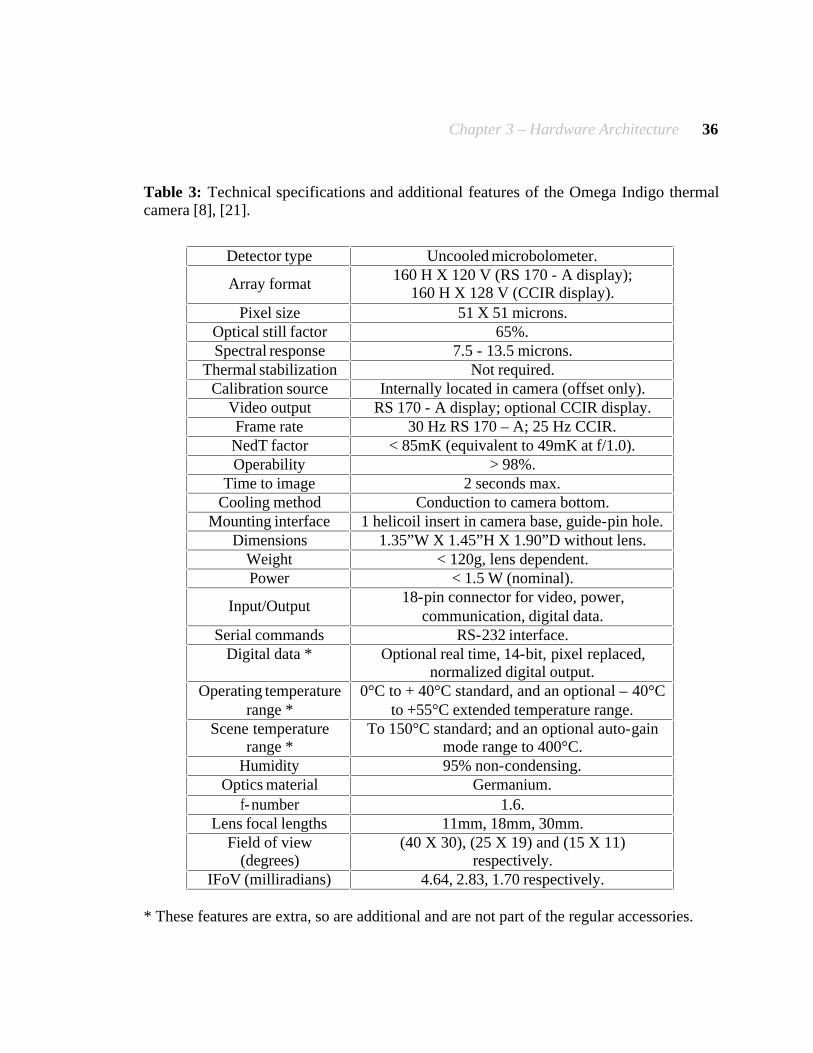
Chapter 3 – Hardware Architecture 36
Table 3: Technical specifications and additional features of the Omega Indigo thermal camera [8], [21].
Detector type Uncooled microbolometer.
Array format 160 H X 120 V (RS 170 - A display);
160 H X 128 V (CCIR display). Pixel size 51 X 51 microns.
Optical still factor 65%. Spectral response 7.5 - 13.5 microns.
Thermal stabilization Not required. Calibration source Internally located in camera (offset only).
Video output RS 170 - A display; optional CCIR display. Frame rate 30 Hz RS 170 – A; 25 Hz CCIR. NedT factor < 85mK (equivalent to 49mK at f/1.0). Operability > 98%.
Time to image 2 seconds max. Cooling method Conduction to camera bottom.
Mounting interface 1 helicoil insert in camera base, guide-pin hole. Dimensions 1.35”W X 1.45”H X 1.90”D without lens.
Weight < 120g, lens dependent. Power < 1.5 W (nominal).
Input/Output 18-pin connector for video, power,
communication, digital data. Serial commands RS-232 interface.
Digital data *
Optional real time, 14-bit, pixel replaced, normalized digital output.
Operating temperature range *
0°C to + 40°C standard, and an optional – 40°C to +55°C extended temperature range.
Scene temperature range *
To 150°C standard; and an optional auto-gain mode range to 400°C.
Humidity 95% non-condensing. Optics material Germanium.
f-number 1.6. Lens focal lengths 11mm, 18mm, 30mm.
Field of view (degrees)
(40 X 30), (25 X 19) and (15 X 11) respectively.
IFoV (milliradians) 4.64, 2.83, 1.70 respectively. * These features are extra, so are additional and are not part of the regular accessories.
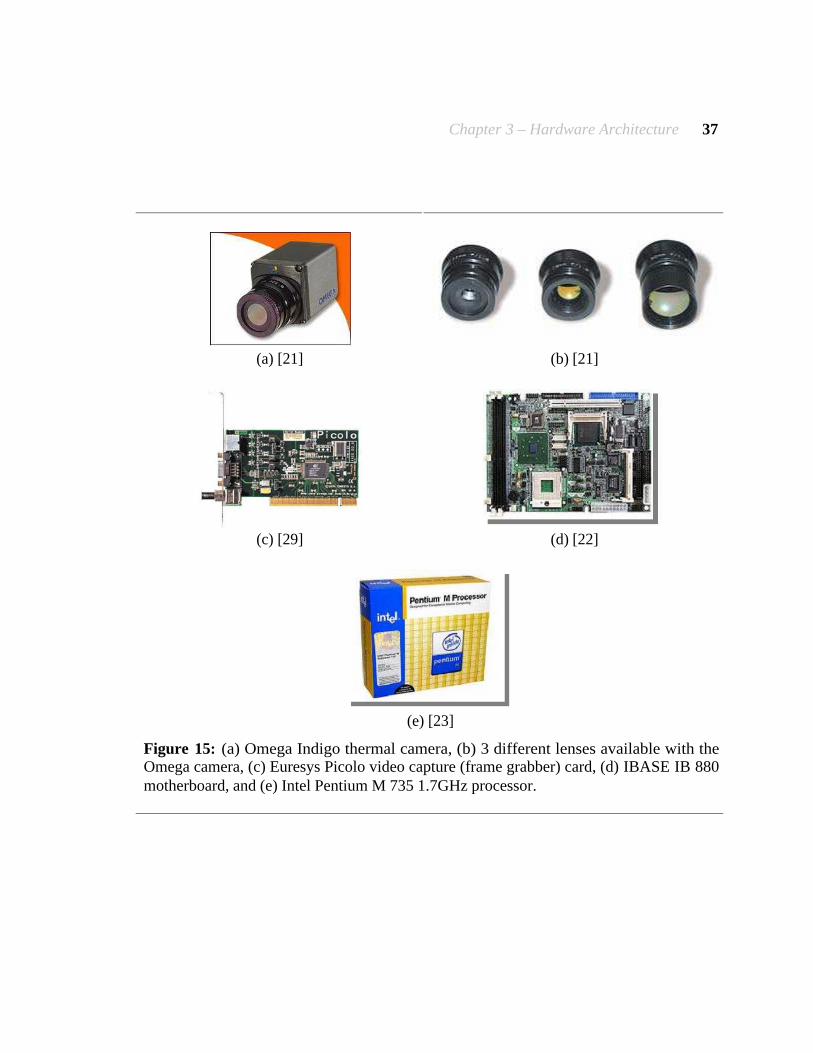
Chapter 3 – Hardware Architecture 37
(a) [21] (b) [21]
(c) [29] (d) [22]
(e) [23]
Figure 15: (a) Omega Indigo thermal camera, (b) 3 different lenses available with the Omega camera, (c) Euresys Picolo video capture (frame grabber) card, (d) IBASE IB 880 motherboard, and (e) Intel Pentium M 735 1.7GHz processor.

Chapter 3 – Hardware Architecture 38
Some of the major advantages of the Omega Indigo thermal camera are: Ø The Omega is extremely compact, light in weight and has a fully integrated
design. These features have been achieved by the manufacturer by being successful in producing Vanadium oxide VOx microbolometer detectors along with proprietary on-focal-plane signal processing that helps in obtaining extraordinary image quality and a high level of image resolution [21]. Ø Since the design of the camera makes a total move away from one traditionally
based on thermoelectric (TE) stabilization, this is what allows the camera to operate with extremely low power consumption and also allows it to display the first image in less than 2.0 seconds. The camera also incorporates analog RS 170 – A, as well as 14 - bit digital output [21]. Omega, which is the world’s smallest thermal camera is as good as a larger thermal camera with regards to performance and features that it has got to offer. The Omega that has a 160 X 128 FPA with signal processing, DSP based electronics and real time algorithms can deliver image quality as good as larger arrays which proves that it makes no compromises for its small size [21]. The VOx detectors allow the Omega to use a higher f-number optics thereby helping in reducing costs and weight [21]. Using the standard f/1.6 lens, it can give a NedT of < 80mK, whereas while using an optional f/1.0 lens, this comes down to < 40mK – which is a factor of 3.0 better than other competing technologies [21]. Figure 15 (b) above shows the three different (11mm, 18mm and 30 mm) lenses that can be fitted on the Omega camera. We use the 8mm lens on our system. The Omega has both an analog and a digital output. It is also capable of delivering wide dynamic range (14 - bit) images at real-time video rates (30 fps) for RS 170 – A, or (25 fps) for CCIR [21]. Auto – ranging function of the Omega spots out extremely hot scenes and decides to switch into an extended temperature range mode thereby allowing to image scenes up to 400°C [21]. An internal shutter continuously recalibrates the camera automatically this can be manually overridden. Recalibration helps in process monitoring applications [21]. The analog video output utilizes a feature called “Smart Scene” which helps to enhance picture quality for all the scenes. Smart Scene uses a dynamic, non-linear conversion to process the 14 - bit digital image data into 8 - bit data for analog video [21]. The conversion algorithm automatically adjusts, frame by frame, to maximize the contrast in darker (colder) parts of the frame, while trying to avoid blanking of brighter (hotter) objects in the image frame. The advantage of this feature is that we automatically get a continuously optimized image independent of scene dynamics [21]. The Omega camera also comes in with a proprietary image optimization system that pre-processes the image data, and eliminates the need for temperature stabilization of the array [21]. Image optimization helps in operating over a wider temperature range and the system does not need a TEC, which helps in saving power consumption [21]. Absence of a TEC helps in giving a very fast turn on time that is highly advantageous [21].
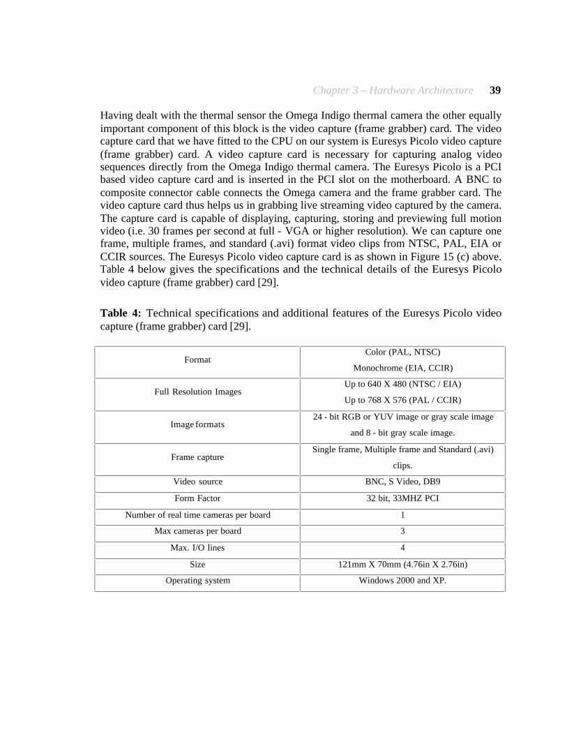
Chapter 3 – Hardware Architecture 39
Having dealt with the thermal sensor the Omega Indigo thermal camera the other equally important component of this block is the video capture (frame grabber) card. The video capture card that we have fitted to the CPU on our system is Euresys Picolo video capture (frame grabber) card. A video capture card is necessary for capturing analog video sequences directly from the Omega Indigo thermal camera. The Euresys Picolo is a PCI based video capture card and is inserted in the PCI slot on the motherboard. A BNC to composite connector cable connects the Omega camera and the frame grabber card. The video capture card thus helps us in grabbing live streaming video captured by the camera. The capture card is capable of displaying, capturing, storing and previewing full motion video (i.e. 30 frames per second at full - VGA or higher resolution). We can capture one frame, multiple frames, and standard (.avi) format video clips from NTSC, PAL, EIA or CCIR sources. The Euresys Picolo video capture card is as shown in Figure 15 (c) above. Table 4 below gives the specifications and the technical details of the Euresys Picolo video capture (frame grabber) card [29].
Table 4: Technical specifications and additional features of the Euresys Picolo video capture (frame grabber) card [29].
Format Color (PAL, NTSC)
Monochrome (EIA, CCIR)
Full Resolution Images Up to 640 X 480 (NTSC / EIA)
Up to 768 X 576 (PAL / CCIR)
Image formats 24 - bit RGB or YUV image or gray scale image
and 8 - bit gray scale image.
Frame capture Single frame, Multiple frame and Standard (.avi)
clips.
Video source BNC, S Video, DB9
Form Factor 32 bit, 33MHZ PCI
Number of real time cameras per board 1
Max cameras per board 3
Max. I/O lines 4
Size 121mm X 70mm (4.76in X 2.76in)
Operating system Windows 2000 and XP.
Chapter 3 – Hardware Architecture 40
3.2 Pre-Processing and Fusion Block
The second block of the TISB system is the Pre - Processing and Fusion block. Here (i.e. on the CPU) the thermal data sensed by the sensor is acquired using the video capture card fitted on the CPU and some low-level image processing operations are performed on the captured data. All the pre - processing is done on the sensor brick CPU and the processed images and the raw data are available to the remotely located host computer for further use. The CPU is the brain of the TISB system and pre-processing software applications add intelligence to it. The TISB system has an IBASE IB 880 motherboard with a 1.7GHz Intel Pentium M 735 processor on it. Figure 15 (d) and (e) above show the motherboard and the processor respectively. Table 5 below lists the technical specifications and configuration of the sensor brick CPU.
3.3 Communication Block
This block of the sensor brick deals with communication between the brick CPU and the host computer situated far away from the sensor brick. Acquired and pre-processed data can be transmitted to the host computer so that it is available for further use and interpretation to users located far away from the sensor brick. Wireless communication is achieved by using 802.11g wireless LAN network adapter card. We have used Intel Pro/Wireless 2915 ABG Network Connection W-LAN adapter that is attached to the half PCI slot on the motherboard. The TISB system has a 2.4Ghz, 5.5-dbi surface mount rubber duck antenna for stronger signal reception. The Intel Pro/Wireless network adapter card and the rubber duck antenna are as shown in Figure 16 (a) and (b) below respectively. The environments we anticipate our brick might have to be placed in while on a search or surveillance mission forced us to go in for the slower but yet highly versatile W-LAN setup using the 802.11g wireless standard. The 802.11g standard employs 54Mbps data rate and is reverse compatible with the 802.11b standard. The modulation technique used in 802.11g standard is called the Orthogonal Frequency Division Multiplexing (OFDM), which is similar to the one used in 802.11a. This is what is mainly responsible for the higher data rates achievable with 802.11g. The operation of 802.11g in the 2.4GHz band and the modulation technique of Complementary Code Keying (CCK) is what makes it similar to the 802.11b and so the 802.11g is reverse compatible with the 802.11b. The 802.11g like the 802.11b has only three non-overlapping channels and hence suffers from interference from other circuits like cordless phones and microwave ovens that also operate in the 2.4GHz range. Ø The 802.11g can achieve a maximum speed of 54Mbps as much as the 802.11a and
5.0 times more then the 802.11b.
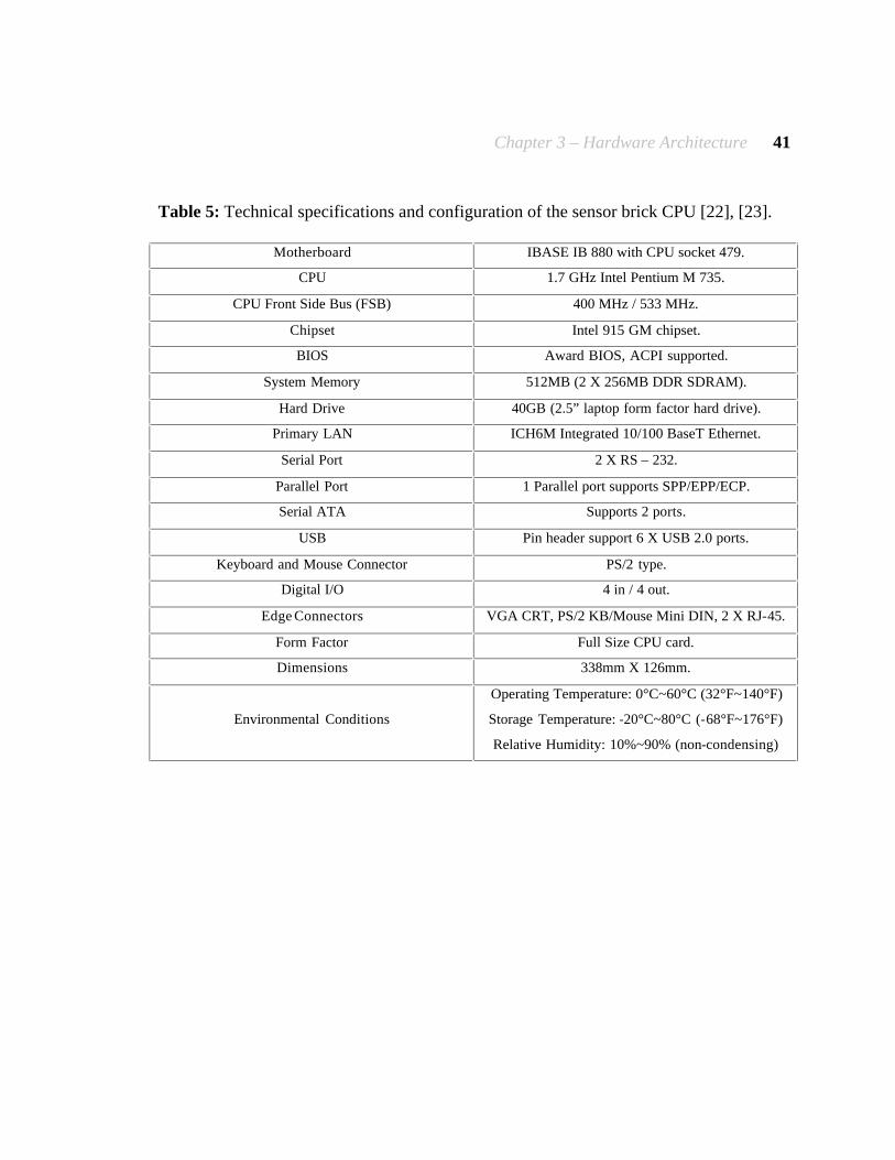
Chapter 3 – Hardware Architecture 41
Table 5: Technical specifications and configuration of the sensor brick CPU [22], [23].
Motherboard IBASE IB 880 with CPU socket 479.
CPU 1.7 GHz Intel Pentium M 735.
CPU Front Side Bus (FSB) 400 MHz / 533 MHz.
Chipset Intel 915 GM chipset.
BIOS Award BIOS, ACPI supported.
System Memory 512MB (2 X 256MB DDR SDRAM).
Hard Drive 40GB (2.5” laptop form factor hard drive).
Primary LAN ICH6M Integrated 10/100 BaseT Ethernet.
Serial Port 2 X RS – 232.
Parallel Port 1 Parallel port supports SPP/EPP/ECP.
Serial ATA Supports 2 ports.
USB Pin header support 6 X USB 2.0 ports.
Keyboard and Mouse Connector PS/2 type.
Digital I/O 4 in / 4 out.
Edge Connectors VGA CRT, PS/2 KB/Mouse Mini DIN, 2 X RJ-45.
Form Factor Full Size CPU card.
Dimensions 338mm X 126mm.
Environmental Conditions
Operating Temperature: 0°C~60°C (32°F~140°F)
Storage Temperature: -20°C~80°C (-68°F~176°F)
Relative Humidity: 10%~90% (non-condensing)

Chapter 3 – Hardware Architecture 42
(a) [23] (b) [24]
(c) [25] (d) [26]
(e) [27] (f) [28]
Figure 16: (a) Intel Pro/Wireless 2915 ABG Network Connection W-LAN adapter, (b) Hyperlink 2.4Ghz, 5.5-dbi RP-SMA rubber duck Antenna, (c) Panasonic LC - RA 1212P a 12V, 12Ah battery, (d) Vicor 12V – 7.5V dc – dc converter for the camera, (e) OPUS 12V, 120W ATX power supply, (f) Astrodyne LPP 150 – 13.5, 120VAC to 12VDC power supply.

Chapter 3 – Hardware Architecture 43
Ø The 802.11g like the 802.11b has a coverage area of 100 – 150 feet inside a room depending on the materials used in the walls as well as the layout of the room, while the 802.11a has a coverage area of only about 25 – 75 feet indoors.
Ø Since 802.11g is reverse compatible with 802.11b a widely used highly compatible
system, hence 802.11g inherits all of 802.11b’s features of public access. Ø The 802.11b is the most widely adopted and hence an inexpensive technology, but
802.11g being new is not that widespread. It is also relatively inexpensive if we weigh the cost against the benefits it has to offer.
Ø The only possible disadvantage of the 802.11g like the 802.11b is it operates in the
crowded 2.4GHz range, so a high risk of interference. On the other hand the 802.11a operates in the uncrowded 5.7GHz range and can coexist with 2.4GHz range circuits without any interference.
3.4 Power Block
Fourth and final block of the TISB system is the Power block. Power supply is the most important factor for continuous and stable operation of the sensor brick. Since the sensor brick has been designed on the concept of modularity and self-sufficiency it needs to exist as a stand-alone system and hence requires its own power setup at all times. Power block provides power to all individual components of the sensor brick. The power block consists of a two connected in parallel 12V, 12Ah Panasonic batteries LC – RA1212P, a 12V – 7.5V dc - dc converter manufactured by Vicor Corporation that powers the camera, OPUS 12V, 120W ATX power supply to power the CPU (motherboard) and Astrodyne LPP 150 – 13.5, 120VAC to 12VDC rectifier to charge the sensor brick batteries. Figure 16 (c) above shows the 12V; 12Ah Panasonic battery LC – RA1212P used as the brick battery, and its technical specifications are given in Table 6 below. Figure 16 (d) above shows the 12V – 7.5V dc - dc converter manufactured by Vicor Corporation, and its technical specifications are given in Table 7 below. Figure 16 (e) above shows the OPUS 12V, 120W ATX power supply to power the CPU (motherboard), and its technical specifications are given in Table 8 below. Figure 16 (f) above shows Astrodyne LPP 150 – 13.5, 120VAC to 12VDC rectifier to charge the sensor brick batteries, and its technical specifications are given in Table 9 below.
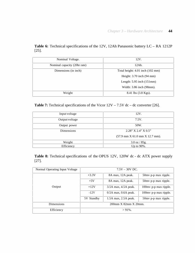
Chapter 3 – Hardware Architecture 44
Table 6: Technical specifications of the 12V, 12Ah Panasonic battery LC – RA 1212P [25].
Nominal Voltage. 12V.
Nominal capacity (20hr rate) 12Ah.
Dimensions (in inch) Total height: 4.01 inch (102 mm)
Height: 3.70 inch (94 mm)
Length: 5.95 inch (151mm)
Width: 3.86 inch (98mm).
Weight 8.41 lbs (3.8 Kgs).
Table 7: Technical specifications of the Vicor 12V – 7.5V dc – dc converter [26].
Input voltage 12V.
Output voltage 7.5V.
Output power 50W.
Dimensions 2.28” X 2.4” X 0.5”
(57.9 mm X 61.0 mm X 12.7 mm).
Weight 3.0 oz / 85g. Efficiency Up to 90%.
Table 8: Technical specifications of the OPUS 12V, 120W dc - dc ATX power supply [27]. Normal Operating Input Voltage 7.5V – 30V DC.
+3.3V 8A max, 12A peak. 50mv p-p max ripple.
+5V 8A max, 12A peak. 50mv p-p max ripple.
+12V 3.5A max, 4.5A peak. 100mv p-p max ripple.
-12V 0.5A max, 0.6A peak. 100mv p-p max ripple.
Output
5V Standby 1.5A max, 2.5A peak. 50mv p-p max ripple.
Dimensions 200mm X 82mm X 20mm.
Efficiency > 91%.

Chapter 3 – Hardware Architecture 45
Table 9: Technical specifications of the Astrodyne LPP 150 – 13.5 120VAC to 12VDC rectifier [28].
Voltage Range: 85 ~ 264VAC.
Frequency Range: 47 ~ 63Hz.
Power Factor: PF ³ 0.96/230VAC,
PF ³ 0.98/115VAC at full load.
Efficiency: 80%.
Input
AC Current: 2.5A/115VAC, 1.2A/230VAC.
DC Voltage: 13.5V.
Rated Current: 11.2A.
Current Range: 0 ~ 11.2A.
Rated Power: 151.2W.
Output
Voltage Adj. Range: 12.8 ~ 14.9V.
Dimensions 222mm X 75mm X 41mm.
Features Short Circuit, Over Load, Over Voltage and Over
Temperature protection.
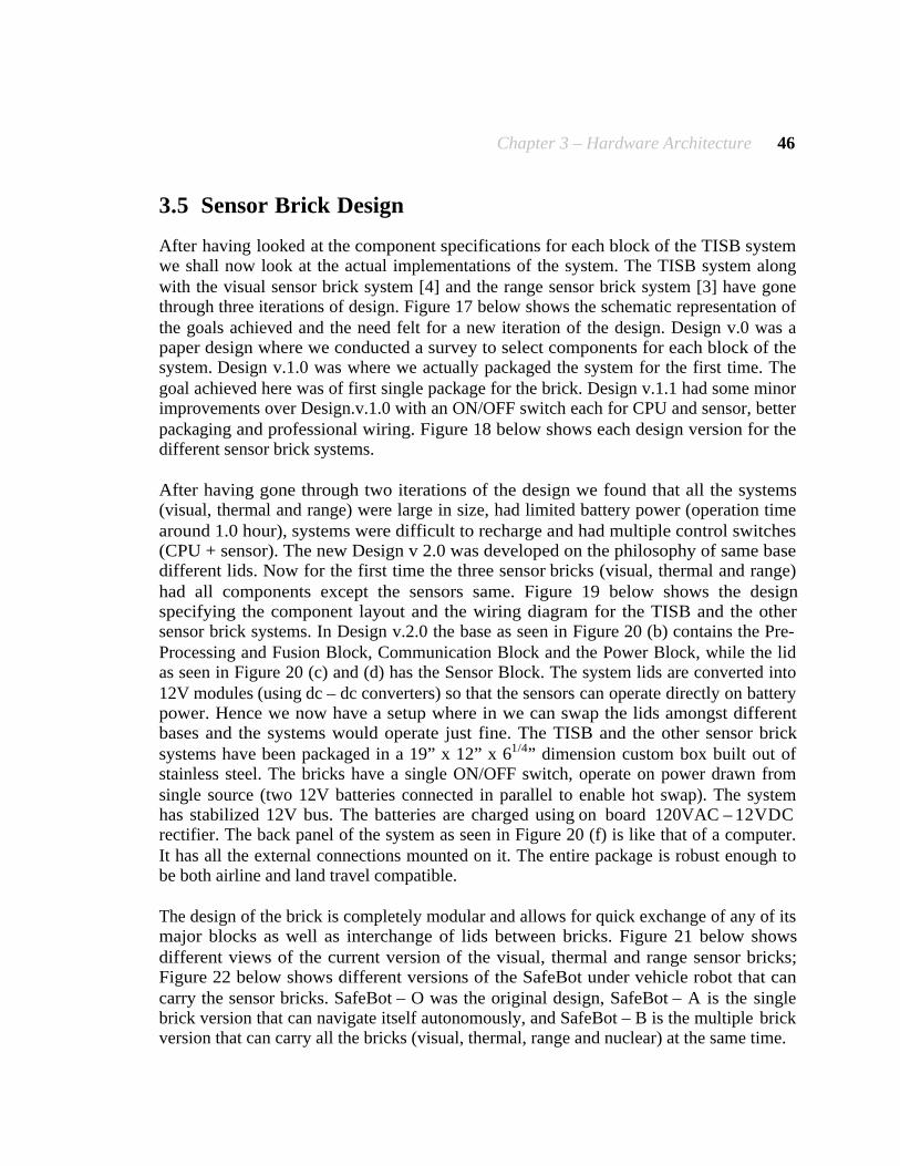
Chapter 3 – Hardware Architecture 46
3.5 Sensor Brick Design
After having looked at the component specifications for each block of the TISB system we shall now look at the actual implementations of the system. The TISB system along with the visual sensor brick system [4] and the range sensor brick system [3] have gone through three iterations of design. Figure 17 below shows the schematic representation of the goals achieved and the need felt for a new iteration of the design. Design v.0 was a paper design where we conducted a survey to select components for each block of the system. Design v.1.0 was where we actually packaged the system for the first time. The goal achieved here was of first single package for the brick. Design v.1.1 had some minor improvements over Design.v.1.0 with an ON/OFF switch each for CPU and sensor, better packaging and professional wiring. Figure 18 below shows each design version for the different sensor brick systems. After having gone through two iterations of the design we found that all the systems (visual, thermal and range) were large in size, had limited battery power (operation time around 1.0 hour), systems were difficult to recharge and had multiple control switches (CPU + sensor). The new Design v 2.0 was developed on the philosophy of same base different lids. Now for the first time the three sensor bricks (visual, thermal and range) had all components except the sensors same. Figure 19 below shows the design specifying the component layout and the wiring diagram for the TISB and the other sensor brick systems. In Design v.2.0 the base as seen in Figure 20 (b) contains the Pre-Processing and Fusion Block, Communication Block and the Power Block, while the lid as seen in Figure 20 (c) and (d) has the Sensor Block. The system lids are converted into 12V modules (using dc – dc converters) so that the sensors can operate directly on battery power. Hence we now have a setup where in we can swap the lids amongst different bases and the systems would operate just fine. The TISB and the other sensor brick systems have been packaged in a 19” x 12” x 61/4” dimension custom box built out of stainless steel. The bricks have a single ON/OFF switch, operate on power drawn from single source (two 12V batteries connected in parallel to enable hot swap). The system has stabilized 12V bus. The batteries are charged using on board 120VAC – 12VDC rectifier. The back panel of the system as seen in Figure 20 (f) is like that of a computer. It has all the external connections mounted on it. The entire package is robust enough to be both airline and land travel compatible. The design of the brick is completely modular and allows for quick exchange of any of its major blocks as well as interchange of lids between bricks. Figure 21 below shows different views of the current version of the visual, thermal and range sensor bricks; Figure 22 below shows different versions of the SafeBot under vehicle robot that can carry the sensor bricks. SafeBot – O was the original design, SafeBot – A is the single brick version that can navigate itself autonomously, and SafeBot – B is the multiple brick version that can carry all the bricks (visual, thermal, range and nuclear) at the same time.
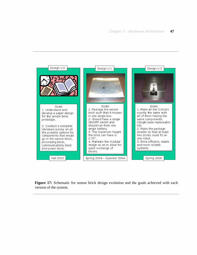
Chapter 3 – Hardware Architecture 47
Figure 17: Schematic for sensor brick design evolution and the goals achieved with each version of the system.

Chapter 3 – Hardware Architecture 48
(a)
(b)
(c)
Figure 18: (a) Visual sensor brick evolution, (b) Thermal sensor brick evolution and, (c) Range sensor brick evolution. For each system we have 3 versions.

Chapter 3 – Hardware Architecture 49
Figure 19: Design specifying the component layout and wiring diagram for the TISB system.
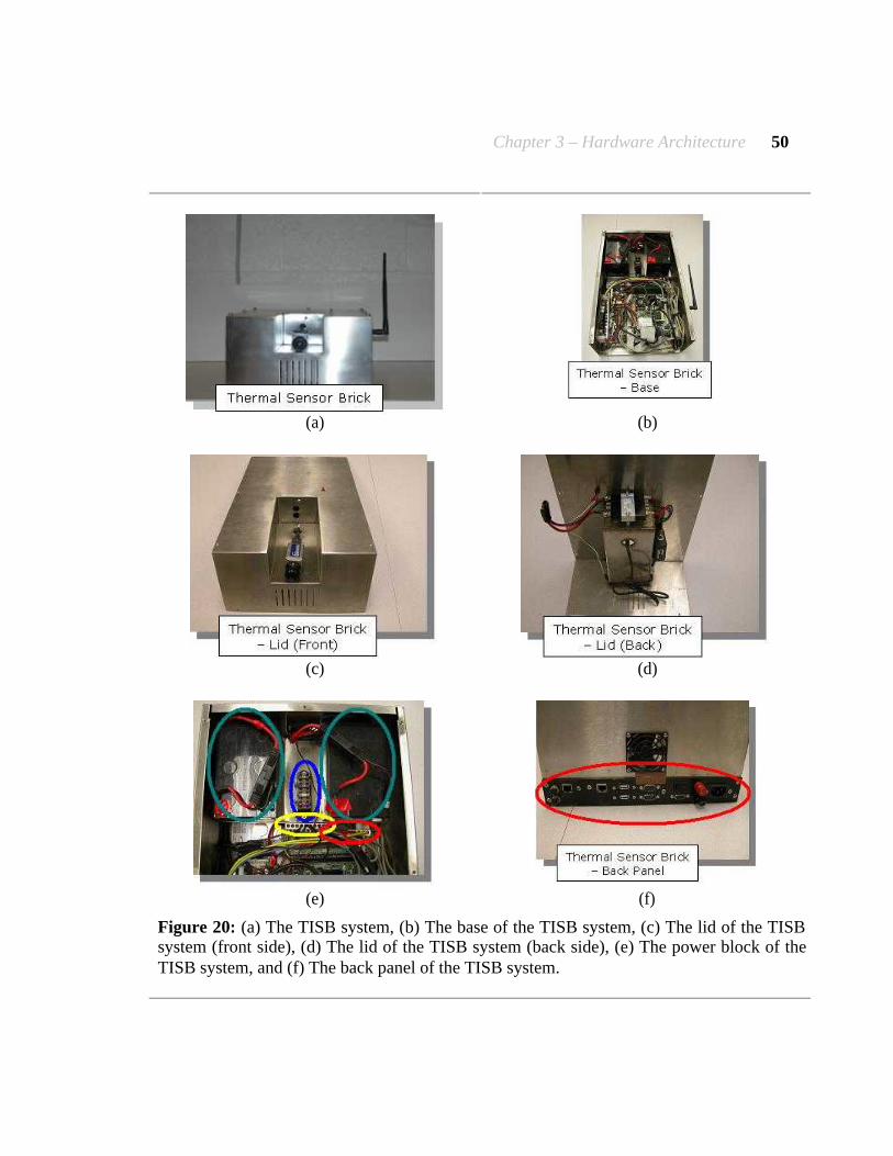
Chapter 3 – Hardware Architecture 50
(a) (b)
(c) (d)
(e) (f)
Figure 20: (a) The TISB system, (b) The base of the TISB system, (c) The lid of the TISB system (front side), (d) The lid of the TISB system (back side), (e) The power block of the TISB system, and (f) The back panel of the TISB system.
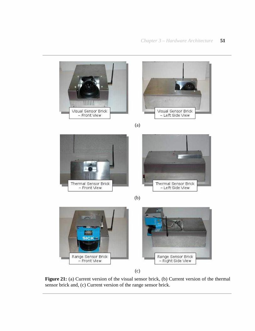
Chapter 3 – Hardware Architecture 51
(a)
(b)
(c)
Figure 21: (a) Current version of the visual sensor brick, (b) Current version of the thermal sensor brick and, (c) Current version of the range sensor brick.
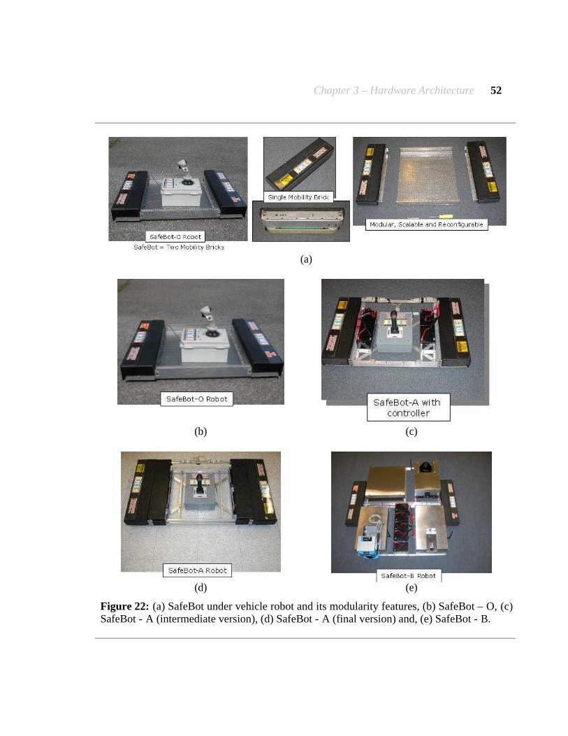
Chapter 3 – Hardware Architecture 52
(a)
(b) (c)
(d) (e)
Figure 22: (a) SafeBot under vehicle robot and its modularity features, (b) SafeBot – O, (c) SafeBot - A (intermediate version), (d) SafeBot - A (final version) and, (e) SafeBot - B.

Chapter 4 – Software Architecture 53
4 Software Architecture
The TISB system has been developed with its main objective being to overcome the shortcomings of a vision based imaging system. In applications such as under vehicle surveillance, area / perimeter surveillance in the dark, or in scenarios where there might not be proper illumination or other factors that normally affect a vision based system are in play our system would be ideally suited. While developing software for our system we have identified some areas of possible application, firstly under vehicle surveillance for threat detection and secondly area / perimeter surveillance with a fixed camera for (Airport surveillance / Nuclear Plant surveillance). In this chapter we shall deal with the software developed for acquisition and processing of thermal data from the TISB system. The TISB system is capable of grabbing data sensed by the thermal sensor (Omega Indigo thermal camera) and displaying it. This data can be captured and saved as a video sequence or as a single frame. The system is capable of capturing full, half and quarter frame sizes. We can also adjust the brightness, contrast, hue and saturation levels for the image. The software allows us to choose between two different types of inputs, either s-video or composite. All the basic Graphical User Interfaces (GUI’s) have been developed using Microsoft DirectX DirectShow software development kit (SDK), which is free and universal and operates at a level that makes the software independent of the hardware. The basic GUI’s help to capture and pre-process data acquired using the TISB system. The TISB system runs on Windows XP as the operating system.
4.1 Acquisition
The TISB system has Euresys Picolo video capture (frame grabber) card on it. This makes the system capable of grabbing data sensed by the thermal sensor and displaying it. The GUI for the TISB system that has been developed by us is dialog based. This GUI allows us to play the streaming video, stop and start it, capture and display a single frame, grab a single frame and save it to a file as a bitmap and also capture the entire stream as an avi video. The layout of this GUI is as seen in Figure 23 below, which shows an image of the screen shot of the working GUI. It consists of 5 sub sections. The first sub-section deals with the acquisition controls and the four other sub-sections deal with the processing controls.

Chapter 4 – Software Architecture 54
Figure 23: Screen shot of the TISB system GUI that has been designed and developed by us in Visual C++ for data acquisition and pre-processing.

Chapter 4 – Software Architecture 55
In this section we shall discuss the data acquisition controls of the GUI. Firstly we need to select the input feed for the data. The tab titled Camera Input allows us to select the camera that we are going to use with this GUI. Since the GUI is universal we can use it with any type of camera and any type of capture card as long as the system identifies the hardware. Once we select the camera we can adjust the camera settings by clicking on the tab titled Camera Settings. This pops up a dialog box that allows us to firstly control the frame size of the input image; our choices are full frame size (640 x 480) pixels, half frame size (320 x 240) pixels and quarter frame size (160 x 120) pixels. Once we have selected the frame size the next window that pops up gives us details about the capture card that is being used and allows us to control the source signal, the data format that we want to use (i.e.) NTSC, PAL, CCIR, EIA and SECAM, the color format (i.e.) Y8 (256 gray scales), RGB 24 and RGB 32, and it also allows us to adjust the image contrast, image brightness, image hue and saturation. Figure 24 below shows a screen shot of the GUI with the popped up window for the above mentioned video source controls. After having set the video controls we need to select the output file to save the grabbed data. Clicking on the tab titled Output Sequence allows us to choose the directory to save the stream as an .avi file. After having selected the output file to save the stream we can choose compression format by clicking on the tab titled Select Compression, which allows us to choose from 32 different compression formats. The compression format commonly used by us for all our data acquisition purposes is MS- MPEG 4 V 2. Now we are ready to acquire and process thermal data as sensed by the Omega Indigo thermal camera. Once we click on the tab titled Process we can see live video feed from the camera in the windows on the left and on the right. The window on the left displays raw data and the window on the right displays processed data. The other controls in this section are Default, which brings back the processed data window to raw data at any point during the operation of the GUI. Stop tab allows us to stop the streaming and processing of the video and the Close tab closes the entire GUI. The tab titled Grab Single Frame allows us to save a single frame or an image as a bitmap file at any point during the operation of the system. This GUI has another tab titled Input Sequence. Instead of displaying and processing live video data if we need to work with already saved data then we can use this tab and select the input video file we want to process, and then perform the same sequence of operations as we would do with a camera input. Only one section of this above mentioned GUI deals with the data acquisition controls. The other GUI that we need to look at in this section is the Omega Camera Control Panel – RS 232 interface software package that we acquired with the camera system. This GUI allows us to control different parameters associated with the camera. The control operations are conducted through RS 232 connection between the camera and the TISB system. We have not developed this GUI but have used it to control camera parameters, which play an important role in our experiments hence we felt the need to explain it here. Figure 25 (a), (b), (c) and (d) shows images of the four different tabs of the GUI respectively.
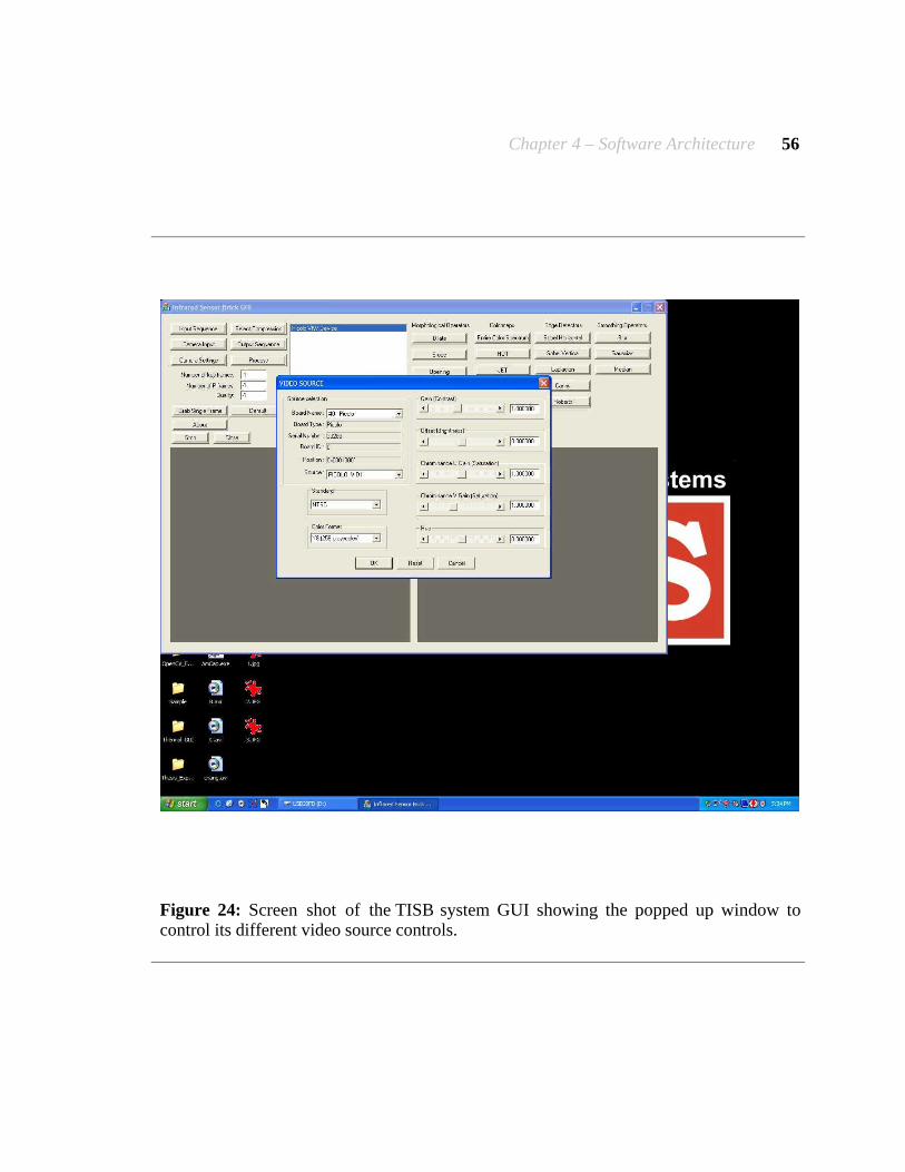
Chapter 4 – Software Architecture 56
Figure 24: Screen shot of the TISB system GUI showing the popped up window to control its different video source controls.

Chapter 4 – Software Architecture 57
(a) [8] (b) [8]
(c) [8] (d) [8]
Figure 25: (a) The General Control section, (b) The Video Control section, (c) The Digital Control section and (d) The Advanced Control section of the Omega Indigo Camera Control Panel – RS 232 interface software package.

Chapter 4 – Software Architecture 58
The window seen in Figure 25 (a) above is displayed when the Control Panel successfully links up with the camera. This GUI has four tabs and six menu options. First is the General tab, this allows us to control three camera parameters. First control is Image Optimization, here is where we can control the camera modes: Smart Scene mode, Auto - Bright mode, Manual mode and Fixed mode [8]. The features of each of these modes have been explained in the Characterization & Experimental Results section. Second is Dynamic Range Control, here we can choose the states of operation of the camera. The low - temperature (high sensitivity) state is intended for imaging scenes that are normally less than 150°C (302°F), the high - temperature (low sensitivity) state is intended for imaging scenes up to 500°C (932°F) and in the Automatic state the camera automatically selects the optimum state between low – temperature and high – temperature based on scene content [8]. The third and the last control on this tab is Flat-Field Correction (FFC), here we can set the FFC to be Manual (i.e. performed as and when we desire) or Automatic (i.e. performed after every 120 seconds or after 1°C change in camera temperature) [8]. Second is the Video tab, this allows us to control five different camera parameters. First control is Video Modes, here is where we can choose to see Real-Time video (i.e.) streaming thermal imagery in real-time, Freeze Frame (i.e.) the camera freezes the frame as soon as this mode is selected and continues to display the same frame from there on, or Disabled which means instead of the thermal imagery we see a uniform gray output [8]. Second control is Test Pattern, we do not use this feature but it allows us to verify the output of the optional digital data channel. In this section our choices are Ascending Ramp test pattern, Vertical Shade pattern or OFF (i.e. no test pattern) [8]. The third control on this tab is Image Orientation; here we can select the image orientation. Normal: is where the pixel on the upper-right corner of the detector array is displayed on the upper-left corner of the video display and Revert: is where the pixel on the upper-left corner of the detector array is displayed on the upper-left corner of the video display [8]. All of our experiments have been conducted with Normal image orientation. Fourth control is Polarity, here we can choose between white-hot or black-hot [8]. All of our experiments have been conducted with white-hot polarity. The fifth and the last control on this tab is Symbology. The Omega camera uses four different on screen symbols for displaying important camera status information. This information is (a) Overtemp: is displayed to indicate that the camera is operating above its maximum specified temperature of 55°C, (b) Low Voltage: displays a battery symbol on the middle left hand side of the screen when the camera input voltage is below 3.5V or (7.5V with extended range), (c) FFC Imminent: displays a small white square on the upper left hand corner of the screen 2.0 seconds before automatic FFC, (d) Low-Sensitivity State: displays a “L” icon on the lower left hand corner of the screen when the camera is in high – temperature (low sensitivity) state [8]. The above-mentioned symbols are displayed based on the mode selection for Symbology. In Black / White mode all icons are displayed in the color of the hot polarity, in Overbright mode all icons are displayed 10% brighter than the brightest white used and in the OFF mode no icons are displayed [8].
Chapter 4 – Software Architecture 59
Third is the Digital tab, this allows us to control the Digital Output (optional digital data channel) of the camera. Here we can choose between 14 - bit data: this data from 164 x 129 pixels is data provided prior to video processing and is the raw data and appears black when saved as an output file, and 8 - bit data: this data from 160 x 120 (NTSC) or 160 x 128 (PAL) is provided after application of image optimization mode, image polarity and image orientation and is the digital version of the actual analog video channel [8]. The fourth and the last tab is the Advanced tab, this allows us to control five different camera parameters. First control is Spotmeter; we do not use this feature [8]. Second control is Temperature scale Fahrenheit or Celsius; we have performed all our experiments using Celsius scale [8]. The third control in this section is Isotherm; we do not use this feature [8]. Fourth control is Camera Temperature; on clicking the button labeled Read we get a read out of the camera case temperature [8]. The fifth and the last control on this tab is Lens; the camera can operate with 11mm, 18mm and 30mm lenses. Since we have only one lens we do not use this feature but this feature allows the camera to switch lenses and based on the selection applies the correct individual lens calibration terms [8]. The Advanced tab has four other controls; Comm Test: is a diagnostic feature to verify the communication link between the Control Panel and the Omega Indigo thermal camera, Save State: allows us to save all the changes effected using the Control Panel as a power up default setting, Reset: as the name suggests reverts to last saved power-up default settings, and lastly Factory Default: restores the camera’s modes and settings to the initial values originally specified by the manufacturer [8]. As mentioned above the Omega Camera Control Panel – RS 232 interface software package also has six menu options. The first menu option is File: this has a single command titled Quit, which allows us to close the Control Panel application [8]. The second menu option is FFC: this executes a manual flat- field correction [8]. The third menu option is Refresh: this updates the Control Panel to reflect all the current settings of the camera [8]. The fourth menu option is Comm: this command allows us to change the communication interface or COM ports for camera communication [8]. The fifth menu option is Image: this allows us to view both 8 - bit and 14 - bit images from the camera and save them as either 8 - bit BMP or 16 – bit TIFF files [8]. The sixth and the last menu option is About: on being clicked this opens an information window that gives us the Control Panel version number, the camera serial number and the camera version number [8].
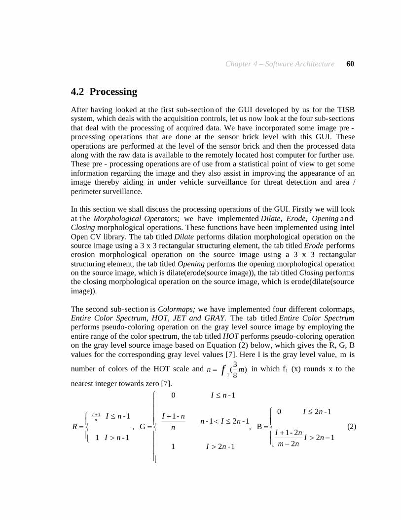
Chapter 4 – Software Architecture 60
4.2 Processing
After having looked at the first sub-section of the GUI developed by us for the TISB system, which deals with the acquisition controls, let us now look at the four sub-sections that deal with the processing of acquired data. We have incorporated some image pre - processing operations that are done at the sensor brick level with this GUI. These operations are performed at the level of the sensor brick and then the processed data along with the raw data is available to the remotely located host computer for further use. These pre - processing operations are of use from a statistical point of view to get some information regarding the image and they also assist in improving the appearance of an image thereby aiding in under vehicle surveillance for threat detection and area / perimeter surveillance. In this section we shall discuss the processing operations of the GUI. Firstly we will look at the Morphological Operators; we have implemented Dilate, Erode, Opening and Closing morphological operations. These functions have been implemented using Intel Open CV library. The tab titled Dilate performs dilation morphological operation on the source image using a 3 x 3 rectangular structuring element, the tab titled Erode performs erosion morphological operation on the source image using a 3 x 3 rectangular structuring element, the tab titled Opening performs the opening morphological operation on the source image, which is dilate(erode(source image)), the tab titled Closing performs the closing morphological operation on the source image, which is erode(dilate(source image)). The second sub-section is Colormaps; we have implemented four different colormaps, Entire Color Spectrum, HOT, JET and GRAY. The tab titled Entire Color Spectrum performs pseudo-coloring operation on the gray level source image by employing the entire range of the color spectrum, the tab titled HOT performs pseudo-coloring operation on the gray level source image based on Equation (2) below, which gives the R, G, B values for the corresponding gray level values [7]. Here I is the gray level value, m is
number of colors of the HOT scale and )8
3(
1mn f= in which f1 (x) rounds x to the
nearest integer towards zero [7].
nInm
n-I
-n I
,
-n I
-nI- nn
n-I
-n I
-n I
-n I
Rn
I
ïïî
ïïí
ì
->-
+
£
=
ïïïï
î
ïïïï
í
ì
>
£<+
£
=ïî
ïí
ì
>
£
=
+
122
2 1
1 20
B
1 21
1 21 1
1 0
G ,
1 1
1 1
(2)
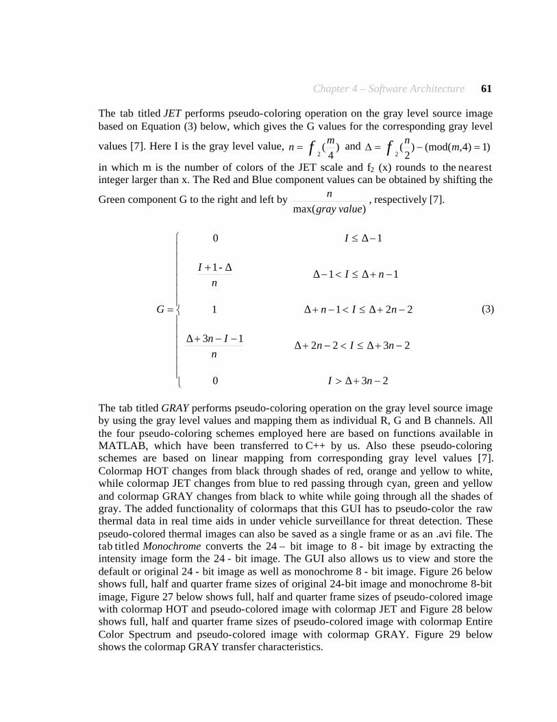
Chapter 4 – Software Architecture 61
The tab titled JET performs pseudo-coloring operation on the gray level source image based on Equation (3) below, which gives the G values for the corresponding gray level
values [7]. Here I is the gray level value, )4
(2
mn f= and )1)4,(mod( )
2(
2=-=D m
nf
in which m is the number of colors of the JET scale and f2 (x) rounds to the nearest integer larger than x. The Red and Blue component values can be obtained by shifting the
Green component G to the right and left by ) max( valuegray
n, respectively [7].
ïïïïïï
î
ïïïïïï
í
ì
-+>
-+£<-+--+
-+£<-+
-+£<-+
-£
=
230
232213
2211
11 1
10
n∆I
n∆In ∆ n
In∆
n∆In ∆
n∆I ∆ n
∆-I
∆ I
G (3)
The tab titled GRAY performs pseudo-coloring operation on the gray level source image by using the gray level values and mapping them as individual R, G and B channels. All the four pseudo-coloring schemes employed here are based on functions available in MATLAB, which have been transferred to C++ by us. Also these pseudo-coloring schemes are based on linear mapping from corresponding gray level values [7]. Colormap HOT changes from black through shades of red, orange and yellow to white, while colormap JET changes from blue to red passing through cyan, green and yellow and colormap GRAY changes from black to white while going through all the shades of gray. The added functionality of colormaps that this GUI has to pseudo-color the raw thermal data in real time aids in under vehicle surveillance for threat detection. These pseudo-colored thermal images can also be saved as a single frame or as an .avi file. The tab titled Monochrome converts the 24 – bit image to 8 - bit image by extracting the intensity image form the 24 - bit image. The GUI also allows us to view and store the default or original 24 - bit image as well as monochrome 8 - bit image. Figure 26 below shows full, half and quarter frame sizes of original 24-bit image and monochrome 8-bit image, Figure 27 below shows full, half and quarter frame sizes of pseudo-colored image with colormap HOT and pseudo-colored image with colormap JET and Figure 28 below shows full, half and quarter frame sizes of pseudo-colored image with colormap Entire Color Spectrum and pseudo-colored image with colormap GRAY. Figure 29 below shows the colormap GRAY transfer characteristics.

Chapter 4 – Software Architecture 62
Figure 26: Top row shows different frame sizes of the original or default data type (24 - bit image). Bottom row shows different frame sizes of the monochrome data (8 - bit image).
Figure 27: Top row shows different frame sizes of the pseudo-colored data with colormap HOT. Bottom row shows different frame sizes of the pseudo-colored data with colormap JET.
Chapter 4 – Software Architecture 63
Figure 28: Top row shows different frame sizes of the pseudo-colored data with colormap Entire Color Spectrum. Bottom row shows different frame sizes of the pseudo-colored data with colormap GRAY.
Figure 29: Colormap GRAY transfer characteristics.
Chapter 4 – Software Architecture 64
Figure 32 (a) and (b) show the transfer characteristics for colormap HOT and JET respectively. We have two more tabs in this sub-section, one labeled Cold Region and the other labeled Hot Region. The function Cold Region only displays those areas in the image that are below the preset intensity threshold, here hot areas are displayed white (intensity level 255) and cold areas are pseudo-colored over the corresponding range of entire color spectrum as shown in Equation (4) below. Similarly Hot Region only displays those areas in the image that are above the preset intensity threshold, here cold areas are displayed black (intensity level 0) and hot areas are pseudo-colored over the corresponding range of entire color spectrum as shown in Equation (5) below. Both of the above mentioned functions perform image segmentation based on intensity threshold level.
þýü
îíì >
=spectrumcolor entire theof range ingcorrespondover color pseudo else
96j)O(i, ;255),(
ifjiPc
(4)
þýü
îíì <
=spectrumcolor entire theof range ingcorrespondover color pseudo else
561j)O(i, ;0),(
ifjiPh
(5)
The value for the threshold in the case of Cold Region is intensity level 96 (i.e. for any given image intensity levels below and equal to 96 are treated as cold regions and all other intensity levels are treated as hot regions). The value for the threshold in the case of Hot Region is intensity level 156 (i.e. for any given image intensity levels above and equal to 156 are treated as hot regions and all other intensity levels are treated as cold regions). The threshold level was selected based on histogram analysis performed on under vehicle surveillance data for threat detection and area / perimeter surveillance data. The purpose of these functions is to let the user know if there is a hot spot in an area where he expects it to be cold and vice-versa if there is a cold spot in an area where he expects it to be hot. Figure 31 below shows an example of Cold Region and Hot Region implementation for the same scene. The third sub-section is Edge Detectors; we have Sobel Horizontal, Sobel Vertical, Laplacian and Canny edge detectors. These functions have been implemented using Intel Open CV library. The tab titled Sobel Horizontal performs edge detection on the source image using a 3 x 3 mask as shown in Equation 6 (a) below to detect the horizontal edges in the image, the tab titled Sobel Vertical performs edge detection on the source image using a 3 x 3 mask as shown in Equation 6 (b) below to detect the vertical edges in the image, the tab titled Laplacian performs edge detection on the source image using a 3 x 3 mask as shown in Equation 6 (c) below to detect all the edges in the image, the tab titled Canny performs edge detection on the source image by the employing the Canny algorithm for edge detection. Figure 30 below shows an example of a source image (Monochrome, 8 - bit) and the corresponding Sobel Horizontal image, Sobel Vertical image, Laplacian image, Canny image and Histogram of the same source image.
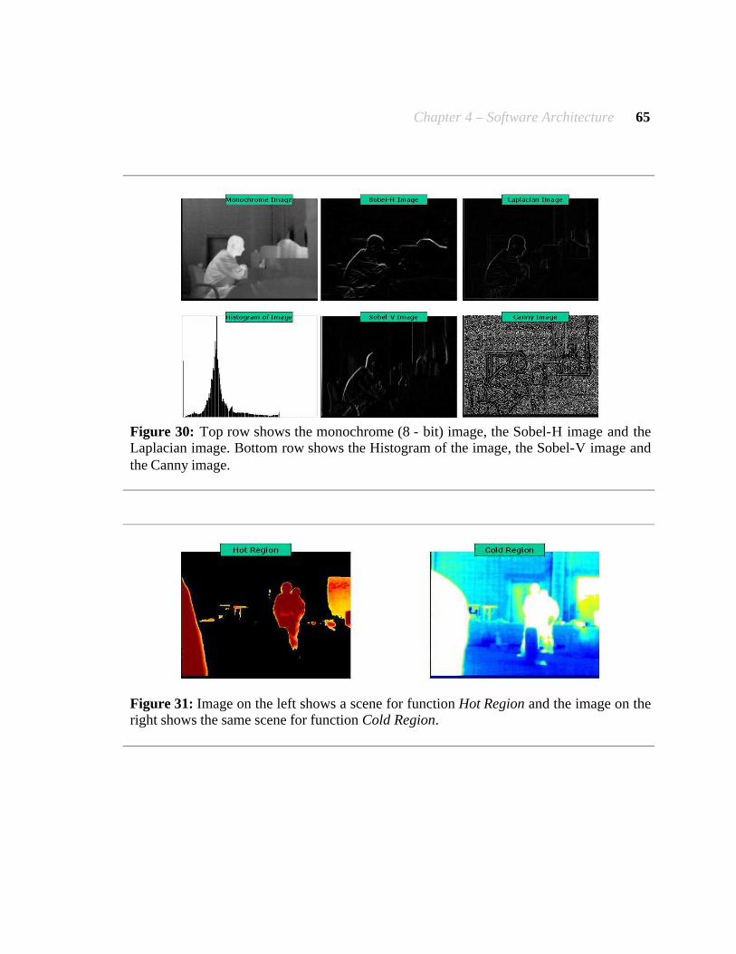
Chapter 4 – Software Architecture 65
Figure 30: Top row shows the monochrome (8 - bit) image, the Sobel-H image and the Laplacian image. Bottom row shows the Histogram of the image, the Sobel-V image and the Canny image.
Figure 31: Image on the left shows a scene for function Hot Region and the image on the right shows the same scene for function Cold Region.

Chapter 4 – Software Architecture 66
(a)
(b)
Figure 32: (a) Colormap HOT transfer characteristics and (b) Colormap JET transfer characteristics.
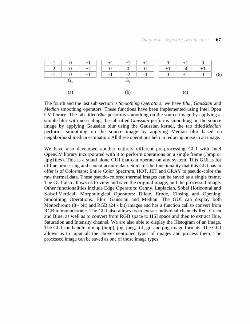
Chapter 4 – Software Architecture 67
-1 0 +1 -2 0 +2 -1 0 +1
Gx
+1 +2 +1 0 0 0 -1 -2 -1
Gy
0 +1 0 +1 -4 +1 0 +1 0
(a) (b) (c)
(6)
The fourth and the last sub section is Smoothing Operators; we have Blur, Gaussian and Median smoothing operators. These functions have been implemented using Intel Open CV library. The tab titled Blur performs smoothing on the source image by applying a simple blur with no scaling, the tab titled Gaussian performs smoothing on the source image by applying Gaussian blur using the Gaussian kernel, the tab titled Median performs smoothing on the source image by applying Median blur based on neighborhood median estimation. All these operations help in reducing noise in an image. We have also developed another entirely different pre-processing GUI with Intel OpenCV library incorporated with it to perform operations on a single frame (.bmp or .jpg files). This is a stand alone GUI that can operate on any system. This GUI is for offline processing and cannot acquire data. Some of the functionality that this GUI has to offer is of Colormaps: Entire Color Spectrum, HOT, JET and GRAY to pseudo-color the raw thermal data. These pseudo-colored thermal images can be saved as a single frame. The GUI also allows us to view and save the original image, and the processed image. Other functionalities include Edge Operators: Canny, Laplacian, Sobel Horizontal and Sobel Vertical; Morphological Operators: Dilate, Erode, Closing and Opening; Smoothing Operations: Blur, Gaussian and Median. The GUI can display both Monochrome (8 - bit) and RGB (24 - bit) images and has a function call to convert from RGB to monochrome. The GUI also allows us to extract individual channels Red, Green and Blue, as well as to convert from RGB space to HSI space and then to extract Hue, Saturation and Intensity channel. We are also able to display the Histogram of an image. The GUI can handle bitmap (bmp), jpg, jpeg, tiff, gif and png image formats. The GUI allows us to input all the above-mentioned types of images and process them. The processed image can be saved as one of those image types.
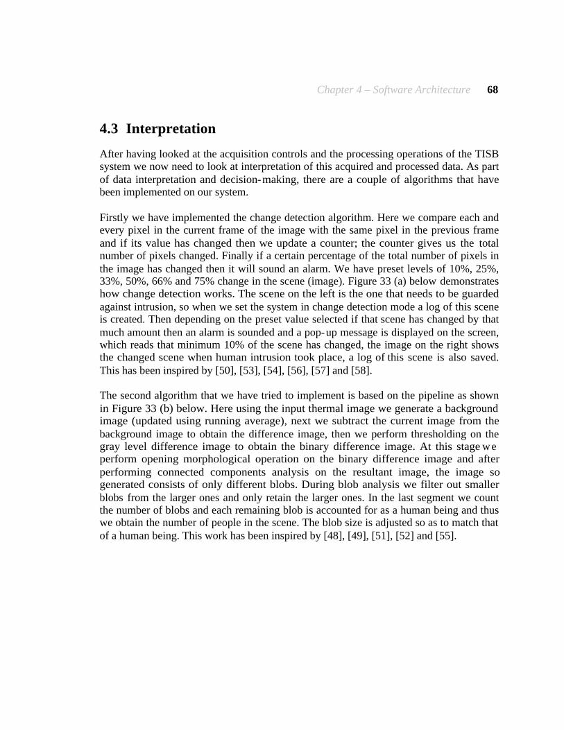
Chapter 4 – Software Architecture 68
4.3 Interpretation
After having looked at the acquisition controls and the processing operations of the TISB system we now need to look at interpretation of this acquired and processed data. As part of data interpretation and decision-making, there are a couple of algorithms that have been implemented on our system. Firstly we have implemented the change detection algorithm. Here we compare each and every pixel in the current frame of the image with the same pixel in the previous frame and if its value has changed then we update a counter; the counter gives us the total number of pixels changed. Finally if a certain percentage of the total number of pixels in the image has changed then it will sound an alarm. We have preset levels of 10%, 25%, 33%, 50%, 66% and 75% change in the scene (image). Figure 33 (a) below demonstrates how change detection works. The scene on the left is the one that needs to be guarded against intrusion, so when we set the system in change detection mode a log of this scene is created. Then depending on the preset value selected if that scene has changed by that much amount then an alarm is sounded and a pop-up message is displayed on the screen, which reads that minimum 10% of the scene has changed, the image on the right shows the changed scene when human intrusion took place, a log of this scene is also saved. This has been inspired by [50], [53], [54], [56], [57] and [58]. The second algorithm that we have tried to implement is based on the pipeline as shown in Figure 33 (b) below. Here using the input thermal image we generate a background image (updated using running average), next we subtract the current image from the background image to obtain the difference image, then we perform thresholding on the gray level difference image to obtain the binary difference image. At this stage we perform opening morphological operation on the binary difference image and after performing connected components analysis on the resultant image, the image so generated consists of only different blobs. During blob analysis we filter out smaller blobs from the larger ones and only retain the larger ones. In the last segment we count the number of blobs and each remaining blob is accounted for as a human being and thus we obtain the number of people in the scene. The blob size is adjusted so as to match that of a human being. This work has been inspired by [48], [49], [51], [52] and [55].

Chapter 4 – Software Architecture 69
(a)
(b)
Figure 33: (a) The results obtained for the change detection algorithm, (b) The pipeline of the proposed algorithm for decision-making based on data interpretation.

Chapter 5 – Characterization & Experimental Results 70
5 Characterization & Experimental Results
Having dealt with the Hardware and the Software Architecture in Chapter 3 and Chapter 4 respectively, we shall look at some of the experimentation conducted as part of this thesis. The major contribution of this thesis is the characterization of the TISB system. We have classified the experiments as hardware experiments where we display the results obtained from analysis conducted to characterize the main blocks of the TISB system. The Sensing and Image Acquisition Block in this case the Omega Indigo thermal camera, the Pre-Processing and Fusion Block (i.e.) the CPU, and the Power Block. Under scenario experiments we have some results demonstrating the application of the TISB system for under vehicle surveillance for threat detection, we shall display all the results obtained based on the experiments conducted and then draw some conclusions based on them.
5.1 Hardware Experiments
5.1.1 Sensing and Image Acquisition Block
As we are already aware the Sensing and Image Acquisition Block of the system consists of the Omega Indigo thermal camera. We conducted the below described experiments to characterize the sensor with the purpose that while capturing data using our thermal sensor we could point at a pixel in the thermal image and estimate its corresponding temperature measurement.
5.1.1.1 Description of the preliminary experiment
The Omega Indigo thermal camera has four image optimization modes namely the Smart Scene mode, the Auto- Bright mode, the Manual mode and the Fixed mode. For each of these modes the settings for the image contrast (0 - 255), image brightness (0 - 16383) and brightness bias (-2047 – 2047) can be adjusted. In the Smart Scene mode the user has no control over the three image parameters and the camera automatically optimizes these image parameters based on the scene content. In the Auto-Bias mode the user can adjust the contrast and the brightness bias but there is no control over the brightness and it is optimized automatically with variations in the scene content, for a given set of values for brightness bias and contrast the most optimal brightness values are automatically selected by the camera. In the Manual mode the user can adjust the contrast and the brightness, the camera automatically optimizes the values of the brightness while entering this mode but this value remains constant and is not continuously updated with changes in scene content or changes in camera temperature. Brightness bias is not used in this mode. In the Fixed mode the user can adjust the contrast and the brightness, these values remain
Chapter 5 – Characterization & Experimental Results 71
constant and are not continuously updated with changes in scene content or changes in camera temperature. Brightness bias is not used in this mode. When switched into this mode the camera uses the last saved values for contrast and brightness as initial values. The preliminary experiments conducted were to decide which image optimization mode is the best in our case. The experimental setup was as shown in Figure 34 below, the scene consisted of four different temperature sources; a paraffin wax bath at 55°C, a cup of hot water on a hot plate at 50°C, an ice pack at 2°C and lastly an object at room temperature around 20°C.
5.1.1.2 Observations for preliminary experiment
The same scene was imaged for each image optimization mode. It was noticed that when a cold object (closer to 0°C) or a hot object (closer to 100°C) was introduced in the scene momentarily the pixel intensity levels tended to change for the Smart Scene mode as seen in Figure 35 and the Auto-Bias mode as seen in Figure 36 but there was no such change in intensity levels for the Manual mode as seen in Figure 37 and the Fixed mode as seen in Figure 38. This was as expected since the Smart Scene mode and the Auto-Bias mode optimizes the image contrast and brightness values to adjust the picture quality. As a result of this we concluded that we could not use the Smart Scene mode and the Auto-Bias mode for our experimentation. We had to decide between the Manual mode and the Fixed mode.
5.1.1.3 Description of Experiment 1
The next set of experiments conducted was to decide which image optimization mode to use, we had to choose between Manual mode and Fixed mode. The experimental setup was as shown in Figure 39 below, the scene consisted of a chair with an object at room temperature around 20°C and an area of the room.
5.1.1.4 Observations for Experiment 1
For Experiment 1A the scene that was imaged is as seen in Figure 39 below, the camera was in the Manual mode, the contrast was set to 100 and the brightness was at 8428, room temperature was 21.7°C. The camera was switched ON instantly and the scene was not fixed (with variations), as seen in Figure 40 below, we noticed that within first ten minutes of the experiment the camera temperature changed by 10°C almost at the rate of 1°C/min and there were variations in average pixel intensity for the entire image. Average pixel intensity for the image is used as a measure of the scene temperature in terms of pixel intensity values. Since the scene temperature was not changing the expectation was that the average pixel intensity for the entire image should remain constant, but this was not the case. Since there were too many parameters that were variable in this experiment we could not draw any conclusion out of this experiment and we decided to conduct the same experiment again with some tighter constraints.
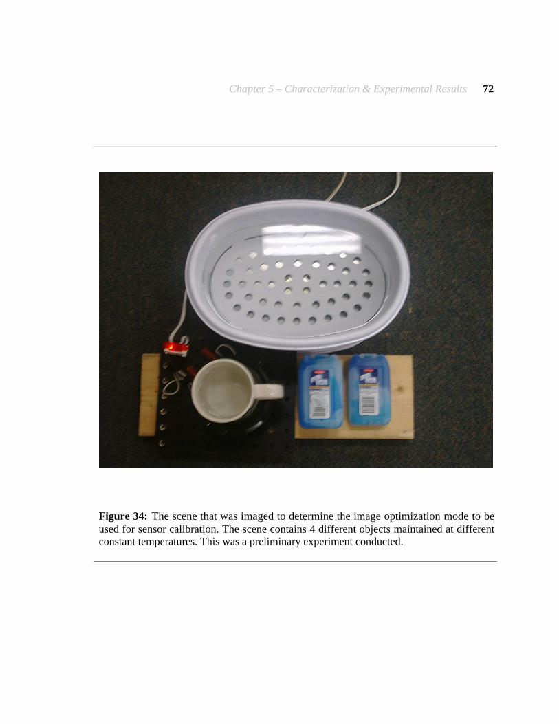
Chapter 5 – Characterization & Experimental Results 72
Figure 34: The scene that was imaged to determine the image optimization mode to be used for sensor calibration. The scene contains 4 different objects maintained at different constant temperatures. This was a preliminary experiment conducted.

Chapter 5 – Characterization & Experimental Results 73
Original scene. Same scene with a cold object introduced in it. (Rescaled intensities)
Original scene back to normal once the cold object
is withdrawn.
Figure 35: Pseudo-colored thermal images of the imaged scene in Smart Scene mode.
Original scene. Same scene with a cold object introduced in it. (Rescaled intensities)
Original scene back to normal once the cold object
is withdrawn.
Figure 36: Pseudo-colored thermal images of the imaged scene in Auto Bright mode.

Chapter 5 – Characterization & Experimental Results 74
Original scene. Same scene with a cold object introduced in it.
Original scene once the cold object is withdrawn.
Figure 37: Pseudo-colored thermal images of the imaged scene in Manual mode.
Original scene. Same scene with a cold object introduced in it.
Original scene once the cold object is withdrawn.
Figure 38: Pseudo-colored thermal images of the imaged scene in Fixed mode.

Chapter 5 – Characterization & Experimental Results 75
Figure 39: The scene that was imaged to determine between Manual and Fixed image optimization modes, to be used for sensor calibration.

Chapter 5 – Characterization & Experimental Results 76
Figure 40: For Experiment 1A the above graph shows variation in Camera Temperature (in °C) and Scene Temperature (in pixel intensity value) against Time (in minutes) with following parameters kept constant: Mode = Manual, Contrast = 100, Brightness = 8428, Room Temp = 21.7°C. Camera was switched ON instantly and the scene was not fixed (with variations).

Chapter 5 – Characterization & Experimental Results 77
For Experiment 1B the scene that was imaged is as seen in Figure 41 below, this is a more controlled scene and here the temperature can be easily monitored. The camera was in the Manual mode, the contrast was set to 100 and the brightness was at 8428, room temperature was 20.3°C. The camera was switched ON instantly, but just as we mentioned above in this instance the scene was fixed (no variations), as seen in Figure 42 below, this time also we noticed that within the first ten minutes of the experiment the camera temperature changed by 10°C almost at the rate of 1°C/min and so again there were variations in average pixel intensity for the entire image. Since the scene temperature was not changing the expectation was that the average pixel intensity for the entire image should remain constant, but this was not the case. The average pixel intensity for the entire image increased with respect to time and then dropped a little. There was no evolving pattern as such. Since this time the scene temperature was maintained constant, we could conclude that the pixel intensity values varied with time of operation of the camera and were always not the same. The other observation was that when we switched from Experiment 1A to Experiment 1B since the field of view and some other parameters like room temperature had changed over the two experiments, in the Manual mode the camera had automatically adjusted the image brightness to a random value to produce an optimized image. This was as expected, hence we could conclude based on this that Manual mode was not an option for us. Having established by the process of elimination that Fixed mode was our best bet for any sort of camera calibration experiments we conducted Experiment 1C. Here the scene that was imaged was same as in the previous case. The camera was in the Fixed mode, the contrast was set to 100 and the brightness was at 8428, room temperature was 20.6°C. The camera was switched ON instantly and the scene was fixed (no variations), as seen in Figure 43 below, this time also we noticed that within the first ten minutes of the experiment the camera temperature changed by 10°C almost at the rate of 1°C/min and there were variations in average pixel intensity for the entire image. Since the scene temperature was not changing the expectation was that the average pixel intensity for the entire image should remain constant, but this was not the case. The average pixel intensity for the entire image increased with respect to time and then dropped a little. There was no evolving pattern as such. Since this time too the scene temperature was maintained constant we could conclude that the pixel intensity values varied with time of operation of the camera and were not the same always. We repeated the same experiment again. For Experiment 1D the scene that was imaged was the same as in the previous case. The camera was in the Fixed mode, the contrast was set to 100 and the brightness was at 8428, room temperature was 16°C. The camera was switched ON instantly and the scene was fixed (no variations), as seen in Figure 44 below, as expected by now this time too we noticed that within the first 10 minutes of the experiment the camera temperature changed by 10°C almost at the rate of 1°C/min and there were variations in average pixel intensity for the entire image, again the average pixel intensity for the entire image increased with respect to time and then dropped.

Chapter 5 – Characterization & Experimental Results 78
Figure 41: The scene that was imaged to determine between Manual and Fixed image optimization modes, to be used for sensor calibration. This was a fixed scene with its temperature being monitored.

Chapter 5 – Characterization & Experimental Results 79
Figure 42: For Experiment 1B the above graph shows variation in Camera Temperature (in °C) and Scene Temperature (in pixel intensity value) against Time (in minutes) with following parameters kept constant: Mode = Manual, Contrast = 100, Brightness = 8428, Room Temp = 20.3°C. Camera was switched ON instantly and the scene was fixed (no variations).
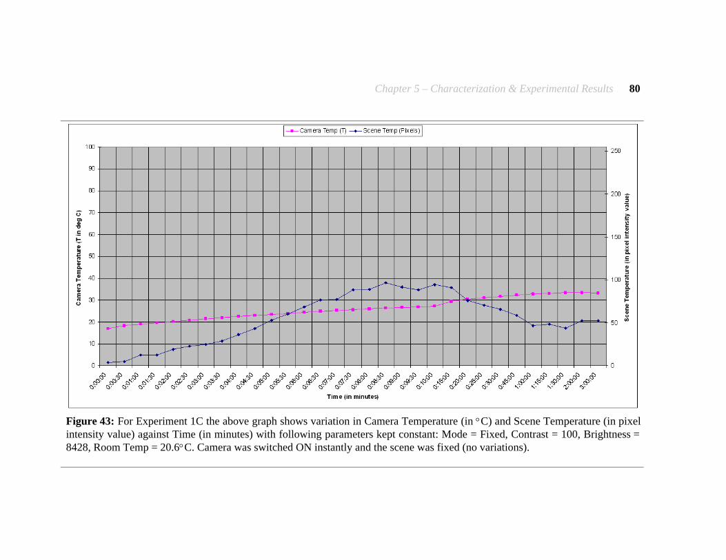
Chapter 5 – Characterization & Experimental Results 80
Figure 43: For Experiment 1C the above graph shows variation in Camera Temperature (in °C) and Scene Temperature (in pixel intensity value) against Time (in minutes) with following parameters kept constant: Mode = Fixed, Contrast = 100, Brightness = 8428, Room Temp = 20.6°C. Camera was switched ON instantly and the scene was fixed (no variations).
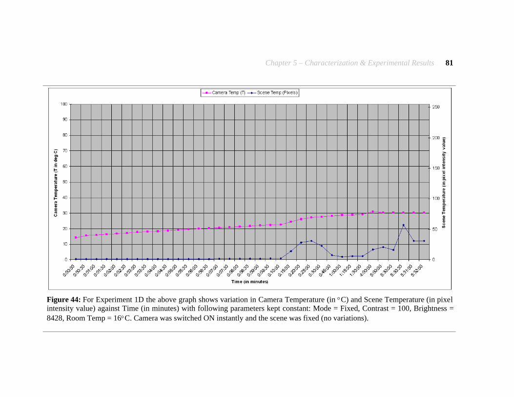
Chapter 5 – Characterization & Experimental Results 81
Figure 44: For Experiment 1D the above graph shows variation in Camera Temperature (in °C) and Scene Temperature (in pixel intensity value) against Time (in minutes) with following parameters kept constant: Mode = Fixed, Contrast = 100, Brightness = 8428, Room Temp = 16°C. Camera was switched ON instantly and the scene was fixed (no variations).
Chapter 5 – Characterization & Experimental Results 82
This time we observed that when we switched from Experiment 1C to Experiment 1D even though the room temperature had changed over the two experiments in the Fixed mode the camera had not adjusted the image brightness to some random value to produce an optimized image and the image was still clear. This was as expected, hence we could conclude based on this that Fixed mode was the only useful mode of operation for us but the change in camera temperature within ten minutes of its operation and the resultant change in the average pixel intensity values for the entire image was a cause of some concern. Also we noticed that that camera temperature stabilized after two hours of operation. In trying to solve the problem of camera heating and the resultant change in average pixel intensity values for the entire image we conducted Experiment 1E. Here the scene that was imaged was same as in the previous case. The camera was in the Fixed mode, the contrast was set to 100 and the brightness was at 8428, room temperature was 18.6°C. In this case though the camera was not switched ON instantly instead it had been running for two hours of continuous operation and the scene was fixed (no variations). As seen in Figure 45 below what did we notice this time? The camera temperature had stabilized and so within the first ten minutes of the experiment the camera temperature did not change even by 0.1°C instead it remained constant during the entire duration of the experiment and also there were no variations in average pixel intensity for the entire image. Since the scene temperature was not changing the expectation was that the average pixel intensity for the entire image should remain constant, and as expected this was the case. Hence we could conclusively infer that the camera had a heating time, which in our case as established was about one hour of operation after which there are no variations in camera temperature and as a result the average pixel intensity over the entire image remains constant. The above mentioned five experiments 1 A, B C, D and E were conducted over a period of three days at different time of the day and it was conclusively established that the Fixed mode is the image optimization mode that we need to operate in to perform any of our camera calibration experiments. The reason for settling on contrast value of 100 and brightness value of 8428 is whenever we switched between modes the camera seemed to automatically settle for these values as the most optimum and the image so generated was also very good.
5.1.1.5 Description of Experiment 2
Having established the image optimization mode to be used, the next set of experiments that were conducted was to perform calibration of the Omega Indigo thermal camera. The experimental setup was as shown in Figure 34 above, the scene consisted of four different temperature sources; a paraffin wax bath at 55°C, a cup of hot water on a hot plate at 50°C, an ice pack at 2.5°C and lastly an object at around room temperature 17.5°C.
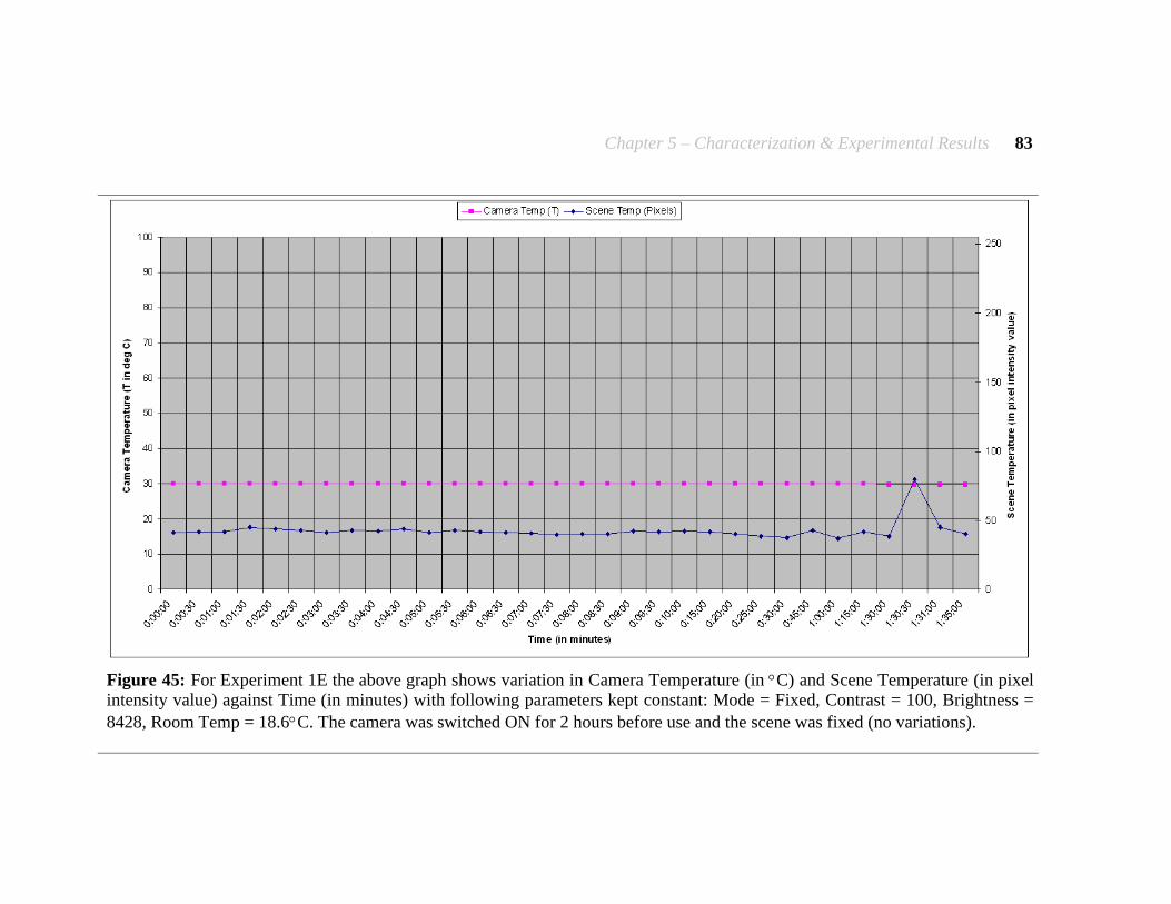
Chapter 5 – Characterization & Experimental Results 83
Figure 45: For Experiment 1E the above graph shows variation in Camera Temperature (in °C) and Scene Temperature (in pixel intensity value) against Time (in minutes) with following parameters kept constant: Mode = Fixed, Contrast = 100, Brightness = 8428, Room Temp = 18.6°C. The camera was switched ON for 2 hours before use and the scene was fixed (no variations).
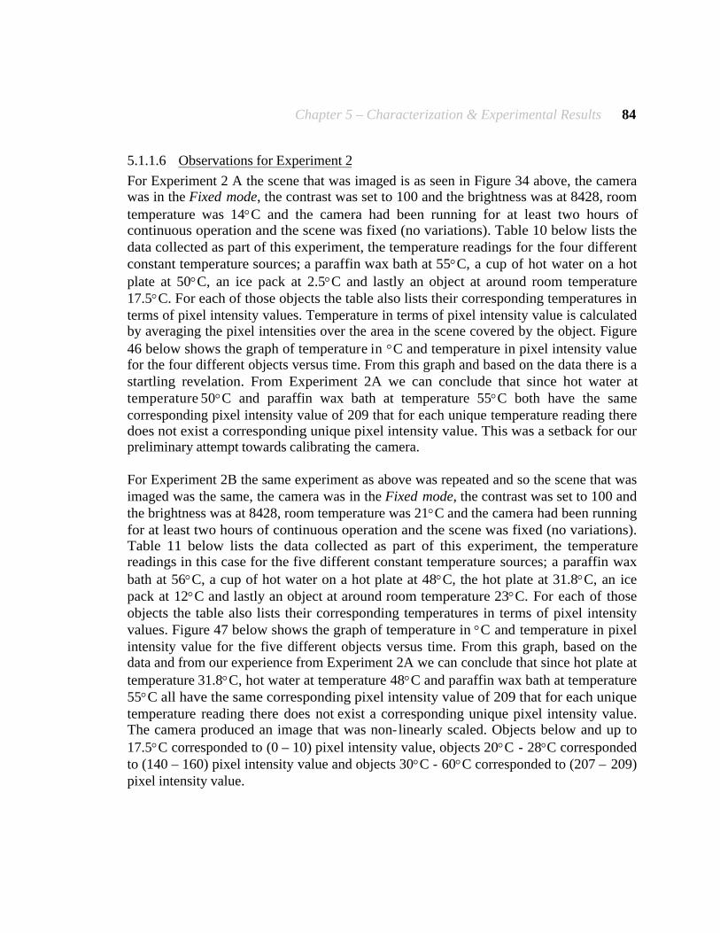
Chapter 5 – Characterization & Experimental Results 84
5.1.1.6 Observations for Experiment 2
For Experiment 2 A the scene that was imaged is as seen in Figure 34 above, the camera was in the Fixed mode, the contrast was set to 100 and the brightness was at 8428, room temperature was 14°C and the camera had been running for at least two hours of continuous operation and the scene was fixed (no variations). Table 10 below lists the data collected as part of this experiment, the temperature readings for the four different constant temperature sources; a paraffin wax bath at 55°C, a cup of hot water on a hot plate at 50°C, an ice pack at 2.5°C and lastly an object at around room temperature 17.5°C. For each of those objects the table also lists their corresponding temperatures in terms of pixel intensity values. Temperature in terms of pixel intensity value is calculated by averaging the pixel intensities over the area in the scene covered by the object. Figure 46 below shows the graph of temperature in °C and temperature in pixel intensity value for the four different objects versus time. From this graph and based on the data there is a startling revelation. From Experiment 2A we can conclude that since hot water at temperature 50°C and paraffin wax bath at temperature 55°C both have the same corresponding pixel intensity value of 209 that for each unique temperature reading there does not exist a corresponding unique pixel intensity value. This was a setback for our preliminary attempt towards calibrating the camera. For Experiment 2B the same experiment as above was repeated and so the scene that was imaged was the same, the camera was in the Fixed mode, the contrast was set to 100 and the brightness was at 8428, room temperature was 21°C and the camera had been running for at least two hours of continuous operation and the scene was fixed (no variations). Table 11 below lists the data collected as part of this experiment, the temperature readings in this case for the five different constant temperature sources; a paraffin wax bath at 56°C, a cup of hot water on a hot plate at 48°C, the hot plate at 31.8°C, an ice pack at 12°C and lastly an object at around room temperature 23°C. For each of those objects the table also lists their corresponding temperatures in terms of pixel intensity values. Figure 47 below shows the graph of temperature in °C and temperature in pixel intensity value for the five different objects versus time. From this graph, based on the data and from our experience from Experiment 2A we can conclude that since hot plate at temperature 31.8°C, hot water at temperature 48°C and paraffin wax bath at temperature 55°C all have the same corresponding pixel intensity value of 209 that for each unique temperature reading there does not exist a corresponding unique pixel intensity value. The camera produced an image that was non- linearly scaled. Objects below and up to 17.5°C corresponded to (0 – 10) pixel intensity value, objects 20°C - 28°C corresponded to (140 – 160) pixel intensity value and objects 30°C - 60°C corresponded to (207 – 209) pixel intensity value.

Chapter 5 – Characterization & Experimental Results 85
Table 10: Temperature readings and the corresponding pixel intensity values for Experiment 2A.
Mode = Fixed, Contrast = 100, Brightness = 8428, Room Temp = 14°C.
Time Camera
Temp (T) °C
Ice Temp (T) °C
Ice Temp (Pixels)
Water Temp
(T) °C Water Temp
(Pixels)
Wax Temp
(T) °C Wax Temp
(Pixels)
Rubber Maid (T) °C
Rubber Maid
(Pixels)
Scene Temp (Pixels)
0:00:00 24.2 2.5 1.1937 50 209.8511 55.5 208.1602 17.5 2.3039 138.9418
0:05:00 24.3 2.5 1.2865 50 210.059 55.5 210.6094 17.5 3.3517 140.0139
0:10:00 24.4 2.5 1.4094 49 210.0206 55.5 210.6168 17.5 12.0912 141.7407
0:15:00 24.4 2.5 1.3155 49 210.0492 55.5 210.6604 17.5 6.6112 140.7109
0:20:00 24.4 2.5 1.3367 48 210.0701 56 210.6048 17.5 4.0781 141.6791
0:25:00 24.4 2.5 1.3224 48 209.9437 55.5 210.8435 17.5 4.6297 141.0841
0:30:00 24.4 2.5 1.3222 48 210.146 55.5 210.6629 17.5 16.5401 146.087
Mean 24.35714286 2.5 1.312342857 48.85714286 210.0199571 55.57142857 210.3082857 17.5 7.086557143 141.4653571
S.D. 0.078679579 0 0.064505319 0.899735411 0.095837447 0.188982237 0.950809649 0 5.268646501 2.260925824
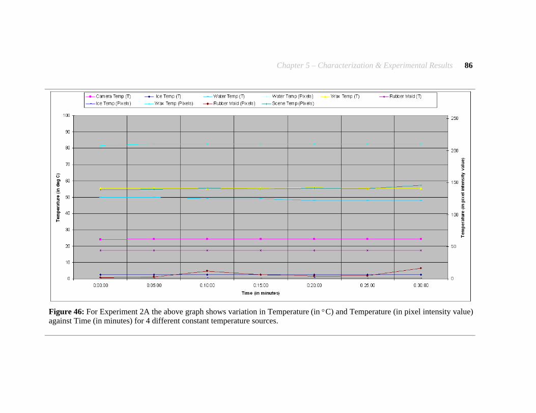
Chapter 5 – Characterization & Experimental Results 86
Figure 46: For Experiment 2A the above graph shows variation in Temperature (in °C) and Temperature (in pixel intensity value) against Time (in minutes) for 4 different constant temperature sources.

Chapter 5 – Characterization & Experimental Results 87
Table 11: Temperature readings and the corresponding pixel intensity values for Experiment 2B.
Mode = Fixed, Contrast = 100, Brightness = 8428, Room Temp = 21°C.
Time Camera
Temp (T) °C Ice Temp
(T) °C Ice Temp (Pixels)
Water Temp
(T)
°C
Water Temp (Pixels)
Wax Temp
(T)
°C
Wax Temp (Pixels)
Rubber Maid (T) °C
Rubber Maid
(Pixels)
Plate Temp
(T)
°C
Plate Temp (Pixels)
Scene Temp (Pixels)
0:00:00 31.8 12.5 1.4104 48 207.4698 56 208.1873 23 167.8087 31.8 207.1996 175.4607
0:05:00 31.6 13 1.2188 48 207.4969 56 208.2792 23 147.0687 31.8 207.2442 172.6617
0:10:00 31.6 13 1.1588 48 207.3448 56 207.9889 23 156.4934 31.8 207.4067 172.9723
0:15:00 31.6 13.5 1.1991 48 207.541 56 208.2411 23 163.7731 31.8 207.3039 174.848
0:20:00 31.6 14 1.187 48 207.6101 56 208.3296 23 145.6533 31.8 207.427 170.7044
0:25:00 31.5 14 1.2836 48 207.3932 56 208.2753 23 156.0417 31.8 207.4028 174.3888
0:30:00 31.5 14.5 1.1836 48 207.3932 56 208.2054 23 166.8046 31.8 207.4025 176.5932
0:30:00 Smart Scene
31.5 14.5 7.1517 48 156.5803 56 182.1929 23 33.181 31.8 71.8151 103.8965
Mean 31.5875 13.625 1.974125 48 201.1036625 56 204.9624625 23 142.1030625 31.8 190.400225 165.1907
S.D. 0.099103121 0.744023809 2.093606715 0 17.99036411 0 9.200863621 0 44.79027501 0 47.91570092 24.83404165
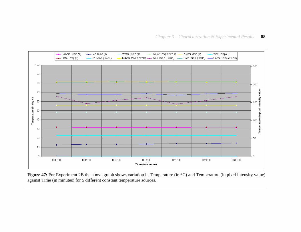
Chapter 5 – Characterization & Experimental Results 88
Figure 47: For Experiment 2B the above graph shows variation in Temperature (in °C) and Temperature (in pixel intensity value) against Time (in minutes) for 5 different constant temperature sources.

Chapter 5 – Characterization & Experimental Results 89
As we can see there is no possible linear relationship between the imaged temperature and the corresponding pixel intensity values. There seems to be a small set of intensity values (0-10) corresponding to temperatures below 17.5°C, then there is a band of intensity values (140-160) corresponding to temperatures 20°C - 2 8 °C, and finally temperatures 30°C – 60°C are packed in a narrow band of intensity values (207 - 209). This gets us to the conclusion that not only is there no linear relationship, but we also noticed that all the intensity values are not represented in the image and there is a very narrow band of intensity values for both hot (30°C - 60°C) and cold (below 17.5°C) objects but a broad band of intensity values for temperatures (20°C - 28°C). There were no reasons to believe that these correspondences between measured temperature and their respective pixel intensity values were based on some formula. It looked like the camera behaved in a random manner every time it was used; the scaling pattern used and the image so generated there by depended on the spectrum of temperatures imaged in the scene. Hence it was getting tougher to suggest a calibration equation, which could transfer temperature in pixel intensity values into temperature in °C.
5.1.1.7 Description of Experiment 3
One of the questions that was raised after the second set of experiments was that maybe the camera did not only image the heat radiated by an object, but also took into consideration the color of the object and the material of the object. This meant that the image generated could possibly be dependent on the material and the color of the object and hence would vary from object to object. The next set of experiments that were conducted was to see if there was any truth in the above doubts based on color and material of an object. The experimental setup was as shown in Figure 48 below, the scene consisted of two different temperature sources; a cup of hot water on a hot plate at 48°C and an ice pack at 7.5°C. We changed the setup by using four cups of different material and color. Figure 48 a, b, c and d show each of the four different setups.
5.1.1.8 Observations for Experiment 3
For Experiment 3 A, B C and D the camera was in the Fixed mode, the contrast was set to 100 and the brightness was at 8428, room temperature was 22°C and the camera had been running for at least two hours of continuous operation and the scene was fixed (no variations). Table 12 and Table 13 below lists the data collected as part of this experiment, the temperature readings for the two constant temperature sources; a cup of hot water on a hot plate at 48°C and an ice pack at 7.5°C for all the four different setups. For each of those setups the tables also list their corresponding temperatures in terms of pixel intensity values. Figure 49, Figure 50, Figure 51 and Figure 52 below each show the graph of temperature in °C and temperature in pixel intensity value for the two different objects versus time for Experiments 3 A, B, C and D respectively.

Chapter 5 – Characterization & Experimental Results 90
(a) (b)
(c) (d)
Figure 48: Images (a), (b), (c) and (d) show the different setups used to for Experiment 3 A, B, C and D respectively to prove that image intensities from the thermal camera do not depend on the color of the object but instead depend directly on its temperature.

Chapter 5 – Characterization & Experimental Results 91
Table 12: Temperature readings and the corresponding pixel intensity values (a) for Experiment 3A and (b) for Experiment 3B.
Mode = Fixed, Contrast = 100, Brightness = 8428, Room Temp = 22°C.
(a)
Time Camera Temp (T)
°C Ice Temp (T) °C Ice Temp (Pixels) Water Temp (T) °C
Water Temp (Pixels)
Scene Temp (Pixels)
0:00:00 31.8 7.5 1.1431 48 207.2556 136.1999
0:05:00 31.8 7.5 1.1462 48 207.3058 136.5616
0:10:00 31.8 7.5 1.1782 48 207.3229 138.1736
0:15:00 31.9 7.5 1.1782 48 207.3808 135.0323
Mean 31.825 7.5 1.161425 48 207.316275 136.49185
S.D. 0.05 0 0.019411401 0 0.05163509 1.297262391
(b)
Time Camera Temp (T)
°C Ice Temp (T) °C Ice Temp (Pixels) Water Temp (T) °C
Water Temp (Pixels)
Scene Temp (Pixels)
0:00:00 32.2 5 1.1269 48 207.3205 134.0064
0:05:00 32.2 5 1.1252 48 207.1811 135.0921
0:10:00 32.2 5 1.5227 48 207.1112 135.3063
0:15:00 32.2 5 1.4993 48 207.1312 137.1213
Mean 32.2 5 1.318525 48 207.186 135.381525
S.D. 0 0 0.222457282 0 0.094361609 1.291925107

Chapter 5 – Characterization & Experimental Results 92
Figure 49: For Experiment 3A the above graph shows variation in Temperature (in °C) and Temperature (in pixel intensity value) against Time (in minutes) for 2 different constant temperature sources as shown in Figure 48 (a).

Chapter 5 – Characterization & Experimental Results 93
Figure 50: For Experiment 3B the above graph shows variation in Temperature (in °C) and Temperature (in pixel intensity value) against Time (in minutes) for 2 different constant temperature sources as shown in Figure 48 (b).

Chapter 5 – Characterization & Experimental Results 94
Table 13: Temperature readings and the corresponding pixel intensity values (a) for Experiment 3C and (b) for Experiment 3D.
Mode = Fixed, Contrast = 100, Brightness = 8428, Room Temp = 22°C.
(a)
Time Camera Temp (T)
°C Ice Temp (T) °C Ice Temp (Pixels) Water Temp (T) °C
Water Temp (Pixels)
Scene Temp (Pixels)
0:00:00 32.2 7.5 1.1303 48 207.1319 129.3651
0:05:00 32.2 7.5 1.1485 48 207.0801 135.0819
0:10:00 32.2 7.5 1.0274 48 207.1778 136.6078
0:15:00 32.2 7.5 1.2517 48 207.1084 138.5305
Mean 32.2 7.5 1.139475 48 207.12455 134.896325
S.D. 0 0 0.091871083 0 0.041336868 3.948217433
(b)
Time Camera Temp (T)
°C Ice Temp (T) °C Ice Temp (Pixels) Water Temp (T) °C Water Temp
(Pixels) Scene Temp
(Pixels)
0:00:00 32.6 7.5 1.1803 48 207.0306 168.7091
0:05:00 32.6 7.5 1.2014 48 206.8835 160.2666
0:10:00 32.6 7.5 1.1255 48 206.9458 161.391
0:15:00 32.6 7.5 1.1195 48 206.8839 156.7049
Mean 32.6 7.5 1.156675 48 206.93595 161.7679
S.D. 0 0 0.040465325 0 0.069560166 5.040177964
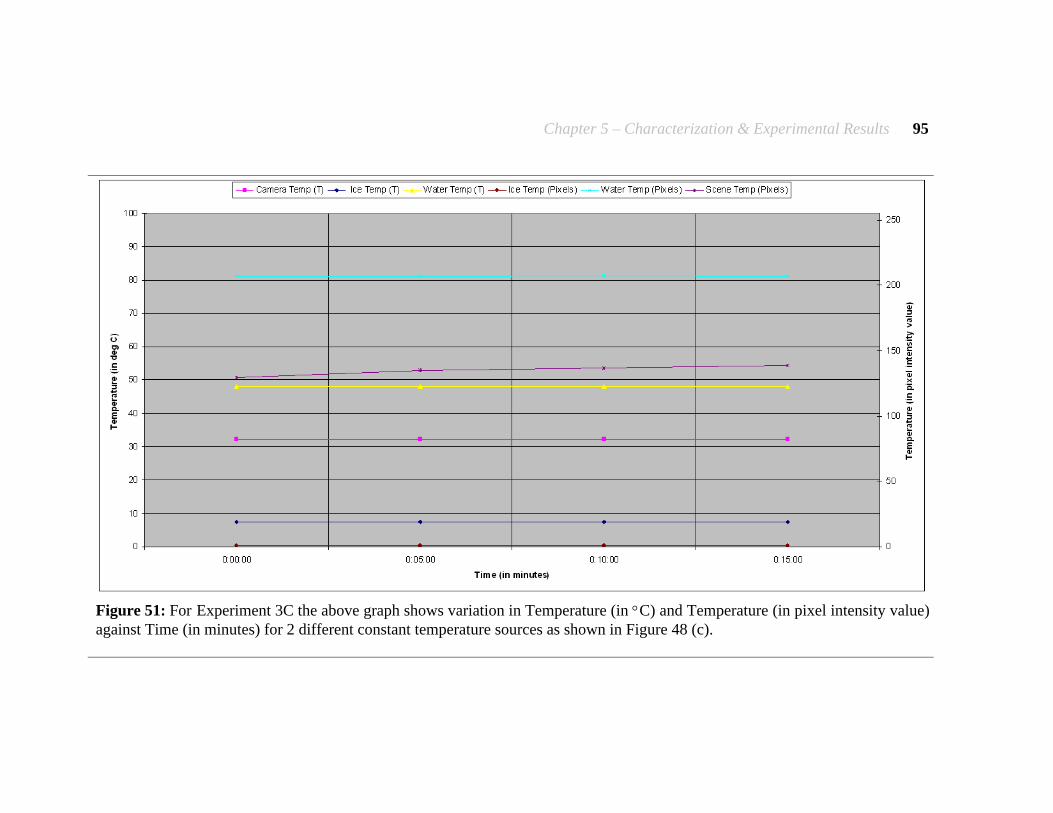
Chapter 5 – Characterization & Experimental Results 95
Figure 51: For Experiment 3C the above graph shows variation in Temperature (in °C) and Temperature (in pixel intensity value) against Time (in minutes) for 2 different constant temperature sources as shown in Figure 48 (c).
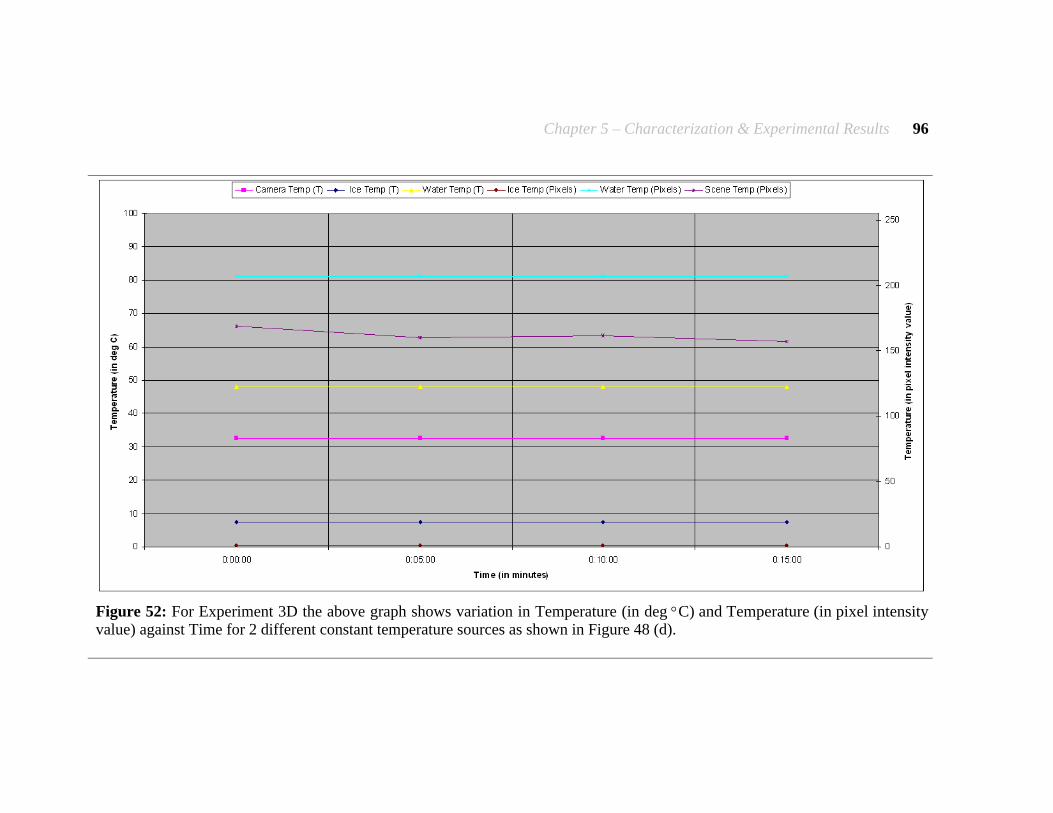
Chapter 5 – Characterization & Experimental Results 96
Figure 52: For Experiment 3D the above graph shows variation in Temperature (in deg °C) and Temperature (in pixel intensity value) against Time for 2 different constant temperature sources as shown in Figure 48 (d).
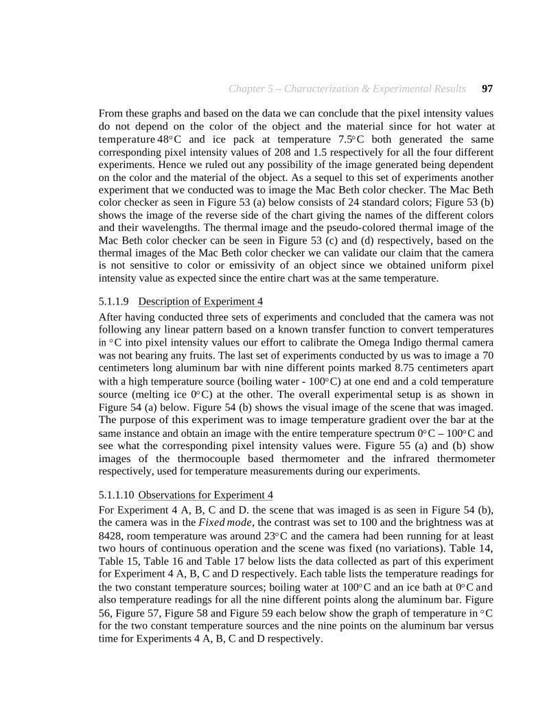
Chapter 5 – Characterization & Experimental Results 97
From these graphs and based on the data we can conclude that the pixel intensity values do not depend on the color of the object and the material since for hot water at temperature 48°C and ice pack at temperature 7.5°C both generated the same corresponding pixel intensity values of 208 and 1.5 respectively for all the four different experiments. Hence we ruled out any possibility of the image generated being dependent on the color and the material of the object. As a sequel to this set of experiments another experiment that we conducted was to image the Mac Beth color checker. The Mac Beth color checker as seen in Figure 53 (a) below consists of 24 standard colors; Figure 53 (b) shows the image of the reverse side of the chart giving the names of the different colors and their wavelengths. The thermal image and the pseudo-colored thermal image of the Mac Beth color checker can be seen in Figure 53 (c) and (d) respectively, based on the thermal images of the Mac Beth color checker we can validate our claim that the camera is not sensitive to color or emissivity of an object since we obtained uniform pixel intensity value as expected since the entire chart was at the same temperature.
5.1.1.9 Description of Experiment 4
After having conducted three sets of experiments and concluded that the camera was not following any linear pattern based on a known transfer function to convert temperatures in °C into pixel intensity values our effort to calibrate the Omega Indigo thermal camera was not bearing any fruits. The last set of experiments conducted by us was to image a 70 centimeters long aluminum bar with nine different points marked 8.75 centimeters apart with a high temperature source (boiling water - 100°C) at one end and a cold temperature source (melting ice 0°C) at the other. The overall experimental setup is as shown in Figure 54 (a) below. Figure 54 (b) shows the visual image of the scene that was imaged. The purpose of this experiment was to image temperature gradient over the bar at the same instance and obtain an image with the entire temperature spectrum 0°C – 100°C and see what the corresponding pixel intensity values were. Figure 55 (a) and (b) show images of the thermocouple based thermometer and the infrared thermometer respectively, used for temperature measurements during our experiments.
5.1.1.10 Observations for Experiment 4
For Experiment 4 A, B, C and D. the scene that was imaged is as seen in Figure 54 (b), the camera was in the Fixed mode, the contrast was set to 100 and the brightness was at 8428, room temperature was around 23°C and the camera had been running for at least two hours of continuous operation and the scene was fixed (no variations). Table 14, Table 15, Table 16 and Table 17 below lists the data collected as part of this experiment for Experiment 4 A, B, C and D respectively. Each table lists the temperature readings for the two constant temperature sources; boiling water at 100°C and an ice bath at 0°C and also temperature readings for all the nine different points along the aluminum bar. Figure 56, Figure 57, Figure 58 and Figure 59 each below show the graph of temperature in °C for the two constant temperature sources and the nine points on the aluminum bar versus time for Experiments 4 A, B, C and D respectively.
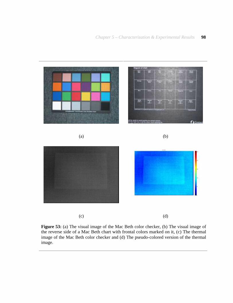
Chapter 5 – Characterization & Experimental Results 98
(a) (b)
(c) (d)
Figure 53: (a) The visual image of the Mac Beth color checker, (b) The visual image of the reverse side of a Mac Beth chart with frontal colors marked on it, (c) The thermal image of the Mac Beth color checker and (d) The pseudo-colored version of the thermal image.
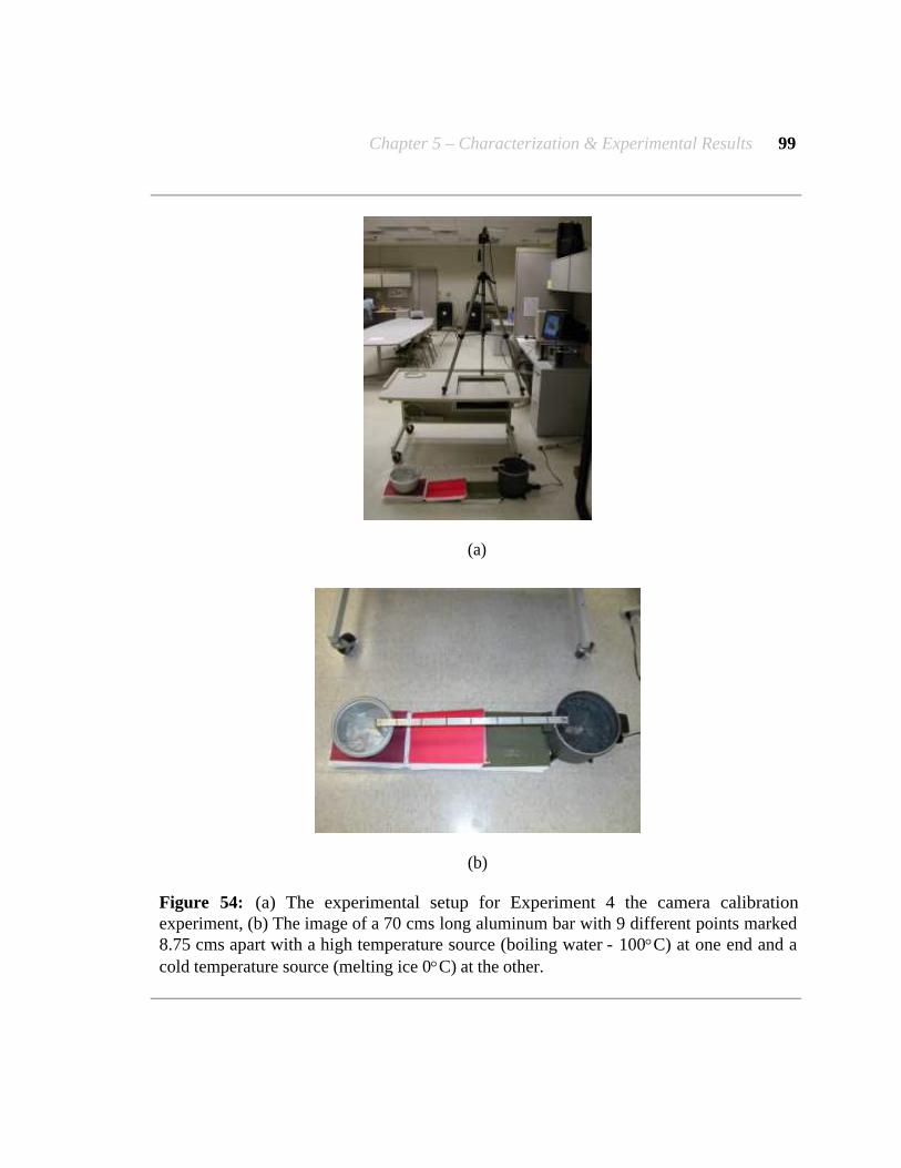
Chapter 5 – Characterization & Experimental Results 99
(a)
(b)
Figure 54: (a) The experimental setup for Experiment 4 the camera calibration experiment, (b) The image of a 70 cms long aluminum bar with 9 different points marked 8.75 cms apart with a high temperature source (boiling water - 100°C) at one end and a cold temperature source (melting ice 0°C) at the other.

Chapter 5 – Characterization & Experimental Results 100
(a)
(b) (c)
Figure 55: (a) The image of the thermocouple-based thermometer used for temperature measurement, (b) The image of an infrared thermometer used for temperature measurement, and (c) The image of an infrared thermometer in operation with the laser pointer pointing at the wall and displaying the reading.
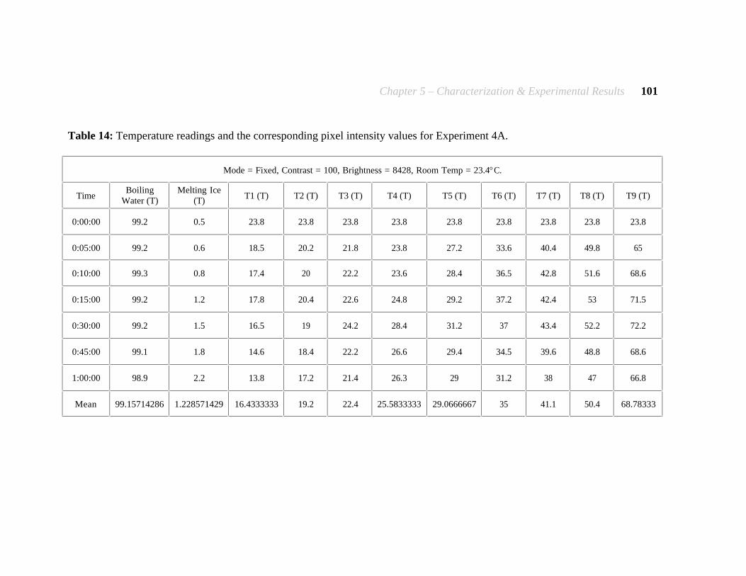
Chapter 5 – Characterization & Experimental Results 101
Table 14: Temperature readings and the corresponding pixel intensity values for Experiment 4A.
Mode = Fixed, Contrast = 100, Brightness = 8428, Room Temp = 23.4°C.
Time Boiling
Water (T) Melting Ice
(T) T1 (T) T2 (T) T3 (T) T4 (T) T5 (T) T6 (T) T7 (T) T8 (T) T9 (T)
0:00:00 99.2 0.5 23.8 23.8 23.8 23.8 23.8 23.8 23.8 23.8 23.8
0:05:00 99.2 0.6 18.5 20.2 21.8 23.8 27.2 33.6 40.4 49.8 65
0:10:00 99.3 0.8 17.4 20 22.2 23.6 28.4 36.5 42.8 51.6 68.6
0:15:00 99.2 1.2 17.8 20.4 22.6 24.8 29.2 37.2 42.4 53 71.5
0:30:00 99.2 1.5 16.5 19 24.2 28.4 31.2 37 43.4 52.2 72.2
0:45:00 99.1 1.8 14.6 18.4 22.2 26.6 29.4 34.5 39.6 48.8 68.6
1:00:00 98.9 2.2 13.8 17.2 21.4 26.3 29 31.2 38 47 66.8
Mean 99.15714286 1.228571429 16.4333333 19.2 22.4 25.5833333 29.0666667 35 41.1 50.4 68.78333
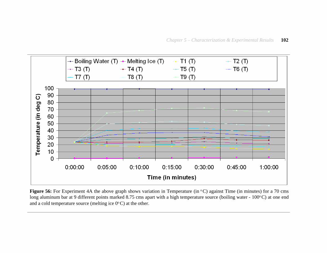
Chapter 5 – Characterization & Experimental Results 102
Figure 56: For Experiment 4A the above graph shows variation in Temperature (in °C) against Time (in minutes) for a 70 cms long aluminum bar at 9 different points marked 8.75 cms apart with a high temperature source (boiling water - 100°C) at one end and a cold temperature source (melting ice 0°C) at the other.

Chapter 5 – Characterization & Experimental Results 103
Table 15: Temperature readings and the corresponding pixel intensity values for Experiment 4B.
Mode = Fixed, Contrast = 100, Brightness = 8428, Room Temp = 23°C.
Time Boiling
Water (T) Melting Ice
(T) T1 (T) T2 (T) T3 (T) T4 (T) T5 (T) T6 (T) T7 (T) T8 (T) T9 (T)
0:00:00 99.5 0.2 23.2 23.2 23.2 23.2 23.2 23.2 23.2 23.2 23.2
0:05:00 99.4 0.4 15.8 18.8 21.2 22.6 25 29.8 41.8 52.5 66.4
0:10:00 99.5 0.6 14.4 18 21.6 23.5 26 32.2 42 53.8 70.4
0:15:00 99.6 0.6 14.2 17.6 21.4 24.8 26.8 36 41.2 54.8 70.6
0:30:00 99.3 0.8 14.6 18.5 22.5 26.8 28 32.8 41.4 50.2 72.2
0:45:00 99.3 1.2 15 18 22.2 27.4 30.2 34 43.8 50.8 70.6
1:00:00 99.3 1.5 15 19.2 23 26 28 33.2 40.2 48.8 68.4
Mean 99.41428571 0.757142857 14.8333333 18.35 21.9833333 25.1833333 27.3333333 33 41.73333 51.81667 69.76667
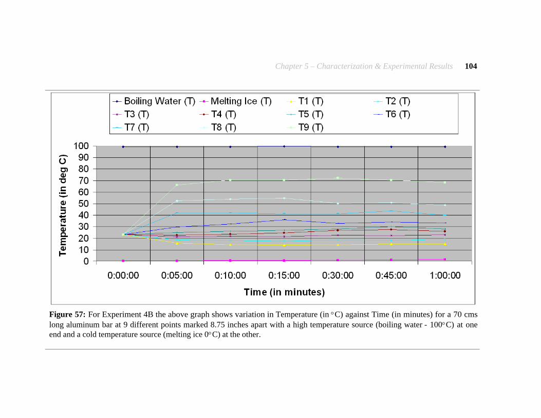
Chapter 5 – Characterization & Experimental Results 104
Figure 57: For Experiment 4B the above graph shows variation in Temperature (in °C) against Time (in minutes) for a 70 cms long aluminum bar at 9 different points marked 8.75 inches apart with a high temperature source (boiling water - 100°C) at one end and a cold temperature source (melting ice 0°C) at the other.

Chapter 5 – Characterization & Experimental Results 105
Table 16: Temperature readings and the corresponding pixel intensity values for Experiment 4C.
Mode = Fixed, Contrast = 100, Brightness = 8428, Room Temp = 23.6°C.
Time Boiling
Water (T) Melting Ice (T)
T1 (T) T2 (T) T3 (T) T4 (T) T5 (T) T6 (T) T7 (T) T8 (T) T9 (T)
0:00:00 99.2 0.1 23.8 23.8 23.8 23.8 23.8 23.8 23.8 23.8 23.8
0:05:00 99.2 0.4 15.8 18.2 20.5 22.6 26.4 32.4 40.8 51.8 71.4
0:10:00 99.3 0.6 16 18.4 21.2 24.6 27.6 34.2 42.6 55 75.5
0:15:00 99.2 0.8 16 19.6 22.6 26.2 29.8 33.8 40.2 52.4 73
0:30:00 99 1 16.8 19.5 23 26.2 28.8 32.2 41.8 52.2 71.4
0:45:00 99.1 1.2 15 18.8 23 25.9 28.8 34.4 42.2 52.8 71.2
1:00:00 98.8 1.5 15.8 18.8 23.4 26.2 30.2 34.2 42.8 51.8 66.4
Mean 99.11428571 0.8 15.9 18.8833333 22.2833333 25.2833333 28.6 33.53333 41.73333 52.66667 71.48333
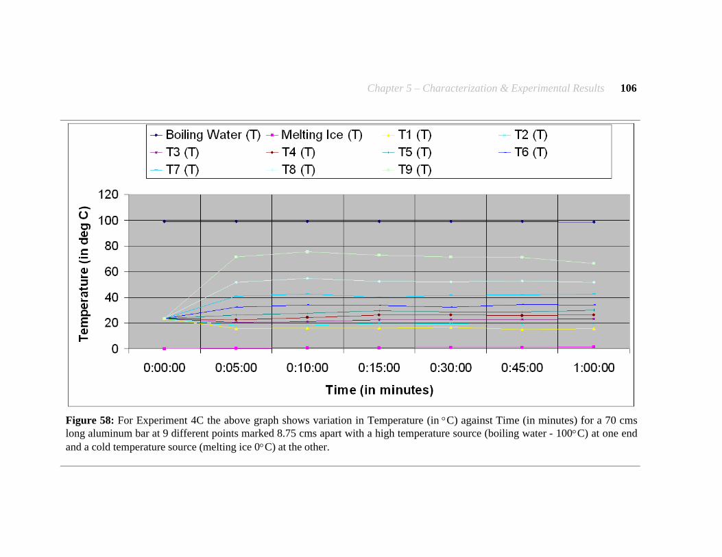
Chapter 5 – Characterization & Experimental Results 106
Figure 58: For Experiment 4C the above graph shows variation in Temperature (in °C) against Time (in minutes) for a 70 cms long aluminum bar at 9 different points marked 8.75 cms apart with a high temperature source (boiling water - 100°C) at one end and a cold temperature source (melting ice 0°C) at the other.
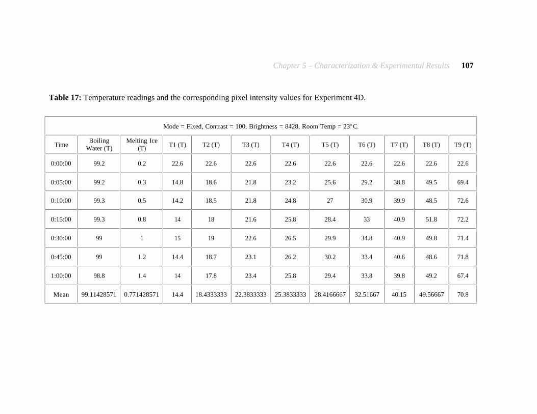
Chapter 5 – Characterization & Experimental Results 107
Table 17: Temperature readings and the corresponding pixel intensity values for Experiment 4D.
Mode = Fixed, Contrast = 100, Brightness = 8428, Room Temp = 23°C.
Time Boiling
Water (T) Melting Ice
(T) T1 (T) T2 (T) T3 (T) T4 (T) T5 (T) T6 (T) T7 (T) T8 (T) T9 (T)
0:00:00 99.2 0.2 22.6 22.6 22.6 22.6 22.6 22.6 22.6 22.6 22.6
0:05:00 99.2 0.3 14.8 18.6 21.8 23.2 25.6 29.2 38.8 49.5 69.4
0:10:00 99.3 0.5 14.2 18.5 21.8 24.8 27 30.9 39.9 48.5 72.6
0:15:00 99.3 0.8 14 18 21.6 25.8 28.4 33 40.9 51.8 72.2
0:30:00 99 1 15 19 22.6 26.5 29.9 34.8 40.9 49.8 71.4
0:45:00 99 1.2 14.4 18.7 23.1 26.2 30.2 33.4 40.6 48.6 71.8
1:00:00 98.8 1.4 14 17.8 23.4 25.8 29.4 33.8 39.8 49.2 67.4
Mean 99.11428571 0.771428571 14.4 18.4333333 22.3833333 25.3833333 28.4166667 32.51667 40.15 49.56667 70.8
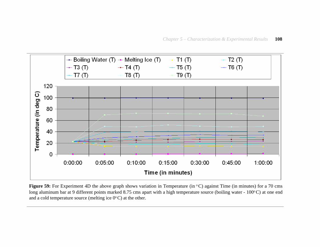
Chapter 5 – Characterization & Experimental Results 108
Figure 59: For Experiment 4D the above graph shows variation in Temperature (in °C) against Time (in minutes) for a 70 cms long aluminum bar at 9 different points marked 8.75 cms apart with a high temperature source (boiling water - 100°C) at one end and a cold temperature source (melting ice 0°C) at the other.
Chapter 5 – Characterization & Experimental Results 109
The above mentioned four experiments 4 A, B, C and D were conducted over a period of two days at different times of the day, and. they all had the same setup. For the first three experiments the imaged scene included the bar and the two constant temperature sources and for the last one the imaged scene included only the bar. This was done to rule out any doubt that, may be the camera scaled its image based on the range of temperatures present in the scene, hence we were trying to avoid extremely hot (100°C) and extremely cold (0°C) in the same scene. After conducting Experiment 4 A, B, C and D we observed that the camera produced an image that was scaled. Objects 0°C - 10°C corresponded to (0 – 10) pixel intensity value, objects 13°C - 31°C corresponded to (140 – 180) pixel intensity value and objects 33°C - 100°C corresponded to (207 – 209) pixel intensity value. Hence it was absolutely clear that there is no possible linear relationship between the imaged temperature and the corresponding pixel intensity values. There is a small set of intensity values (0-10) for temperatures 0°C - 10°C, then there is a band of intensity values (140-180) corresponding to temperatures 13°C - 31°C, and finally temperatures 33°C – 100°C are packed in a narrow band of intensity values (207 - 209). The above results validated our conclusion after Experiment 2 that not only is there no linear relationship, but we had also noticed that all the intensity values were not represented in the image and there was a very narrow band of values for temperature 33°C - 100°C, broad band for temperatures 0°C - 10 °C and a very broad band for temperatures 13°C - 31°C. Figure 60 below shows the plot of temperature (in °C) versus corresponding intensity values for all the four different trials and the mean value for Experiment 4. This plot gives us the camera transfer characteristics. Based on the mean value plot, we tried to approximate the transfer characteristics to a polynomial curve using Microsoft Excel and MATLAB. Our conclusion using both the systems was the same. The transfer curve approximated to a 3rd degree polynomial function. Figure 61 below shows the plot of the mean value curve and the approximated curves obtained using Microsoft EXCEL and MATLAB. The transfer function of the camera is as given in Equation 7 below. Here I is the intensity value (0 - 255) and T is the temperature (in °C). This transfer function gives accurate results with up to 90% accuracy in the temperature range of 15°C - 75°C.
I = 0.0007T3 – 0.1535T2 + 10.399T – 12.8632 (7)
Figure 62 below shows the plot of temperature (in °C) versus distance (in cms) of the measured point from boiling water, while Figure 63 below shows the plot of intensity values versus distance (in cms) of the measured point from boiling water for all the four different trials of the experiment. These plots highlight the temperature gradient across the 70 cms long aluminum bar and the associated variation in corresponding intensity values.

Chapter 5 – Characterization & Experimental Results 110
Figure 60: The above graph shows a plot of Temperature (in °C) versus corresponding Intensity Values for all the 4 different trials of the experiment and the mean value for a 70 cms long aluminum bar with a high temperature source (boiling water - 100°C) at one end and a cold temperature source (melting ice 0°C) at the other. This plot gives us the camera transfer characteristics.
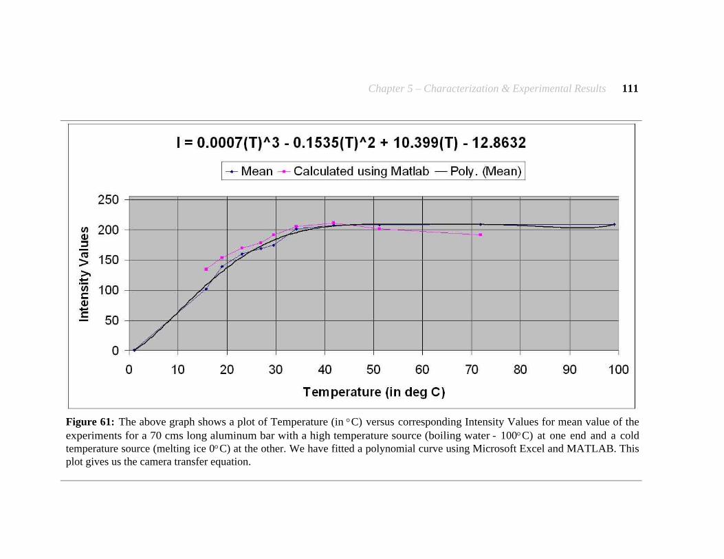
Chapter 5 – Characterization & Experimental Results 111
Figure 61: The above graph shows a plot of Temperature (in °C) versus corresponding Intensity Values for mean value of the experiments for a 70 cms long aluminum bar with a high temperature source (boiling water - 100°C) at one end and a cold temperature source (melting ice 0°C) at the other. We have fitted a polynomial curve using Microsoft Excel and MATLAB. This plot gives us the camera transfer equation.

Chapter 5 – Characterization & Experimental Results 112
Figure 62: The above graph shows a plot of Temperature (in °C) versus Distance (in cms) of the measured point from boiling water for all the 4 different trials of the experiment for a 70 cms long aluminum bar with a high temperature source (boiling water - 100°C) at one end and a cold temperature source (melting ice 0°C) at the other.
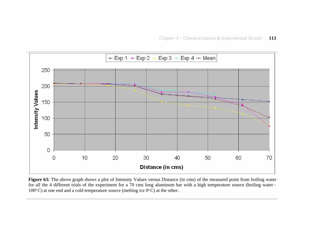
Chapter 5 – Characterization & Experimental Results 113
Figure 63: The above graph shows a plot of Intensity Values versus Distance (in cms) of the measured point from boiling water for all the 4 different trials of the experiment for a 70 cms long aluminum bar with a high temperature source (boiling water - 100°C) at one end and a cold temperature source (melting ice 0°C) at the other.
Chapter 5 – Characterization & Experimental Results 114
5.1.2 Processing Block
As we are already aware the Processing Block of the system consists of the CPU, we have discussed details about the CPU and all its specifications in the chapter on hardware architecture. We performed some analysis of the CPU by running some processes that we expect the CPU to be able to handle and measured its peak load during these processes. The readings so obtained have been tabulated in Table 18 below. The conclusion that we can draw from this experiment is that the current CPU can handle our processing requirements with it average peak CPU load being around 60%. The process of pseudo-coloring the raw thermal data is the most CPU exhaustive process and registers peak CPU load of about 90%. Figure 64, Figure 65 and Figure 66 below show screen shots of the windows task manager used to monitor CPU load displaying variable CPU usage during different operations of the system.
5.1.3 Power Block
After having characterized the Sensor Block and the Processing Block of the TISB system, we performed some analysis on the Power Block of the system. The main component of the Power Block is the 12V; 12Ah (Panasonic LC - RA 1212P) lead acid battery. We have two of these batteries that are being used on the TISB system and they provide for all the power requirements of the system. The details about the battery specifications have been discussed in the chapter on hardware architecture. The analysis that we performed on the battery was to obtain its charge and discharge characteristics for different current ratings. Figure 67, Figure 68 and Figure 69 below, show the brick battery (Panasonic LC-RA 1212P) charge characteristics at 2A, 10A, 12A and 20A respectively. Figure 70 below shows a combined plot of all the four different charge characteristics. Figure 71 and Figure 72 below show the discharge characteristics for the brick battery (Panasonic LC-RA 1212P) at 12A and 24A individually and together on the same plot respectively. Table 19 below, gives us the charge and discharge characteristics for the 12V; 12Ah brick battery for different current ratings. Based on the data in Table 19 below we know that at 2A (trickle charge) the battery requires 346 minutes or 5hours 46 minutes to be charged, at 10A current the battery will charge in 44 minutes, at 12A current in 36 minutes and at 24A current in 24 minutes. The battery discharges completely in 20 minutes at 12A current draw and in 11 minutes at 24A current draw. From experimentation we know that the TISB system can last for 300 minutes or 5.0hours on battery power while operating under its normal condition, this means that it has an average current draw of (0.8A ~ 1.0A).

Chapter 5 – Characterization & Experimental Results 115
Table 18: Peak CPU load readings for different processes and functions employed on the TISB system.
Process Peak CPU load
Starting the Thermal Sensor Brick GUI 12%
Data acquisition operations 41%
Raw thermal image acquisition (Default) 63%
Morphological Operator: Dilate 63%
Morphological Operator: Erode 63%
Morphological Operator: Opening 63%
Morphological Operator: Closing 63%
Colormap: Entire Color Spectrum 92%
Colormap: HOT 88%
Colormap: JET 92%
Colormap: GRAY 82%
Function: Monochrome Image 66%
Function: Cold Region 88%
Function: Hot Region 88%
Edge Operator: Sobel – H 66%
Edge Operator: Sobel – V 69%
Edge Operator: Laplacian 72%
Edge Operator: Canny 88%
Smoothing Operator: Blur 63%
Smoothing Operator: Gaussian 63%
Smoothing Operator: Median 63%
After stopping data acquisition 7%
After exiting the Thermal Sensor Brick GUI 1%
Table 19: Charge and Discharge characteristics of the 12V, 12Ah brick battery (Panasonic LC-RA 1212P) for different current ratings.
Charge Characteristics
Charge Current Time (in Minutes) Time (in Hours)
2A 346 5Hrs 46mins
10A 44 0Hrs 44mins
12A 36 0Hrs 36mins
24A 24 0Hrs 24mins
Discharge Characteristics
Discharge Current Time (in Minutes) Time (in Hours)
12A 20 0Hrs 20mins
24A 11 0Hrs 11mins

Chapter 5 – Characterization & Experimental Results 116
Figure 64: Screen shot of the windows task manager, which shows CPU load of the system while processing data using colormaps.
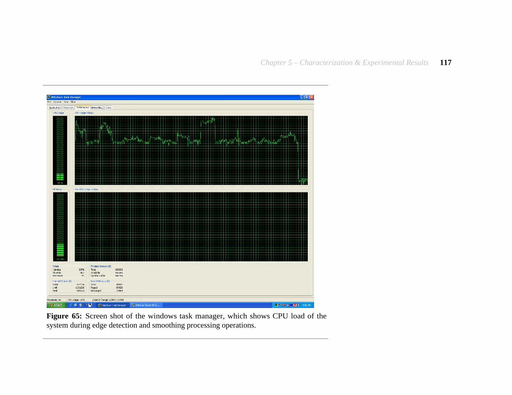
Chapter 5 – Characterization & Experimental Results 117
Figure 65: Screen shot of the windows task manager, which shows CPU load of the system during edge detection and smoothing processing operations.
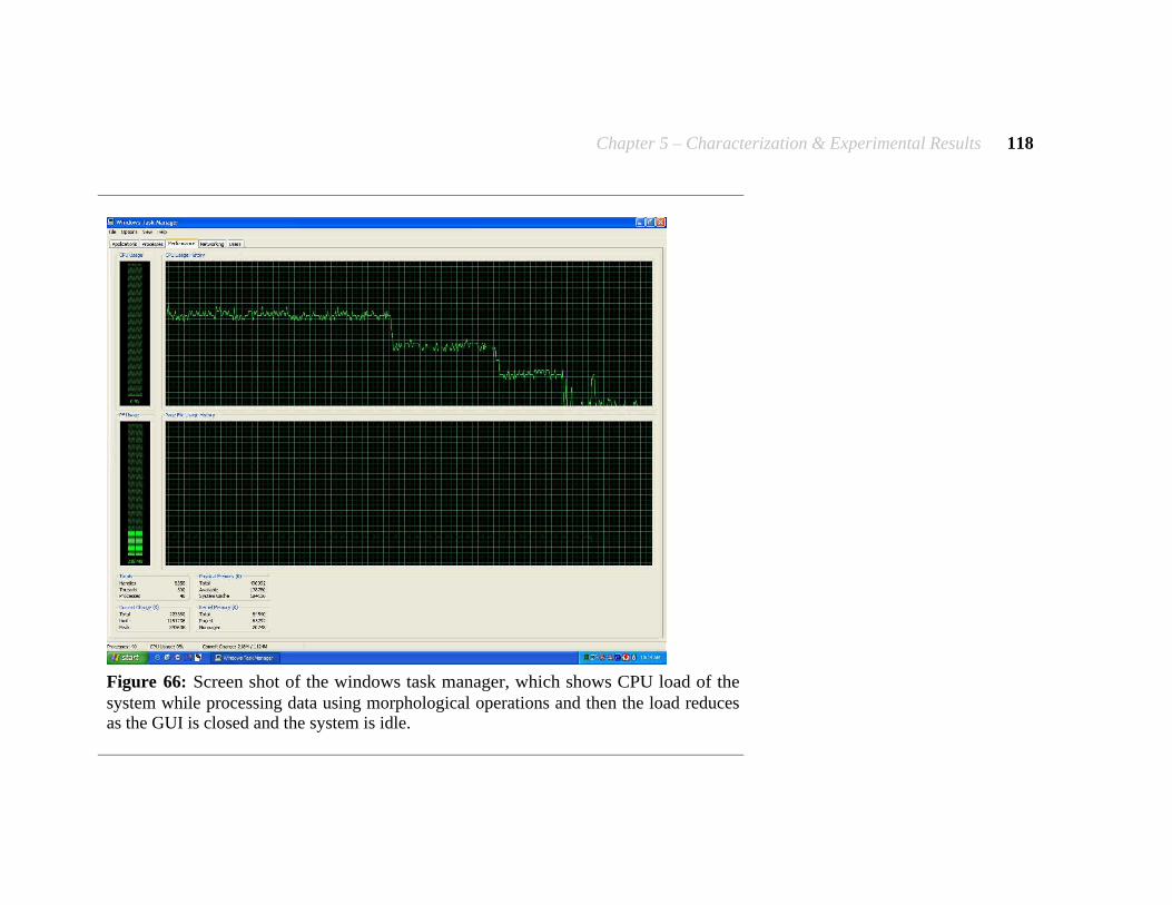
Chapter 5 – Characterization & Experimental Results 118
Figure 66: Screen shot of the windows task manager, which shows CPU load of the system while processing data using morphological operations and then the load reduces as the GUI is closed and the system is idle.

Chapter 5 – Characterization & Experimental Results 119
(a)
(b)
Figure 67: (a) Scaled plot of brick battery (Panasonic LC-RA 1212P) charge characteristics at 2A, (b) Full plot of brick battery (Panasonic LC-RA 1212P) charge characteristics at 2A.

Chapter 5 – Characterization & Experimental Results 120
(a)
(b)
Figure 68: (a) Full plot of brick battery (Panasonic LC-RA 1212P) charge characteristics at 10A, (b) Full plot of brick battery (Panasonic LC-RA 1212P) charge characteristics at 12A.
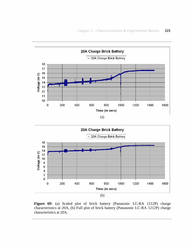
Chapter 5 – Characterization & Experimental Results 121
(a)
(b)
Figure 69: (a) Scaled plot of brick battery (Panasonic LC-RA 1212P) charge characteristics at 20A, (b) Full plot of brick battery (Panasonic LC-RA 1212P) charge characteristics at 20A.

Chapter 5 – Characterization & Experimental Results 122
Figure 70: Full plot of the combined brick battery (Panasonic LC-RA 1212P) charge characteristics, (2A, 10A, 12A, 20A).

Chapter 5 – Characterization & Experimental Results 123
(a)
(b)
Figure 71: (a) Scaled plot of brick battery (Panasonic LC-RA 1212P) discharge characteristics at 12 A, (b) Full plot of brick battery (Panasonic LC-RA 1212P) discharge characteristics at 12A.
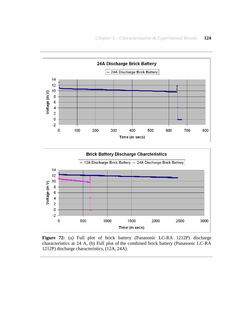
Chapter 5 – Characterization & Experimental Results 124
Figure 72: (a) Full plot of brick battery (Panasonic LC-RA 1212P) discharge characteristics at 24 A, (b) Full plot of the combined brick battery (Panasonic LC-RA 1212P) discharge characteristics, (12A, 24A).

Chapter 5 – Characterization & Experimental Results 125
5.2 Scenario Experiments
One of the main applications of our TISB system is under vehicle surveillance for threat detection. This section demonstrates the advantage of the TISB system over purely vision-based systems. Experiments conducted highlight the advantages of our system being an illumination invariant threat detection system for detecting hidden threat objects in the undercarriage of a car by comparing it to vision sensor brick system and the mirror on a stick. We have also illustrated the capability of the TISB system to be operational when fitted on the SafeBot under vehicle robot to acquire thermal data. The under vehicle scenario experiments were conducted at the UT transportation department using a Ford Taurus car, a Dodge Stratus car and a Dodge RAM 3500 van. Figure 73 below shows the visual, thermal, pseudo-colored thermal and the image as seen with the mirror on a stick of a section of the undercarriage of a van. This dataset tries to highlight the application we have targeted and how our system is better suited.
5.2.1 Under vehicle thermal video sequences (Variation with time)
As part of this experiment we acquired thermal video sequences to look for variations in under vehicle conditions with time for a car engine that has been operational for 30 minutes. Figure 74 below shows the visual, thermal and pseudo-colored thermal images of two different fields of view of the undercarriage of a Dodge RAM 3500 van. Figure 74 (a) shows the section with the catalytic converter and the muffler and Figure 74 (b) shows the section with the muffler and the exhaust pipe. For each field of view the thermal image shown is a single frame of the entire thermal video sequence (0 – 30 minutes) acquired to observe variations with time of under vehicle conditions.
5.2.2 Under vehicle thermal video sequences (Normal or expected results)
As part of this experiment we acquired thermal video sequences to check for normal or expected results and look for a possible hidden / threat object, which may go unnoticed in the visual image but the difference in temperature with its surroundings, may highlight its presence. By expected or normal results we mean that if by common knowledge we know that a certain section is either hot (catalytic converter and muffler) or cold (fuel tank and axle) then on imaging it the results should match our expectations, if not then we can safely assume that something is wrong (suspicious) with that section of the undercarriage. Figure 75 below shows the visual, thermal and pseudo-colored thermal images of the true muffler, which is hot as expected and the false muffler, which is cold, hence is a suspicious object. Figure 76 below shows a combined view of the true muffler and the false muffler in the same field of view, and also an overall view showing how the thermal image of the undercarriage of the van that has been operational should look (as expected).
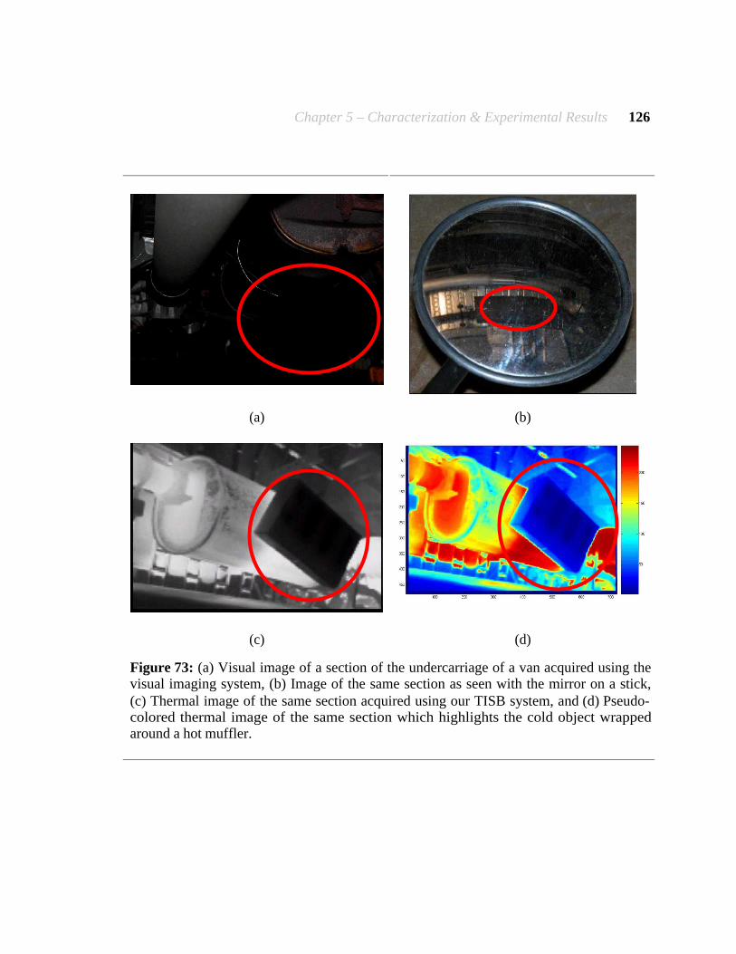
Chapter 5 – Characterization & Experimental Results 126
(a) (b)
(c) (d)
Figure 73: (a) Visual image of a section of the undercarriage of a van acquired using the visual imaging system, (b) Image of the same section as seen with the mirror on a stick, (c) Thermal image of the same section acquired using our TISB system, and (d) Pseudo-colored thermal image of the same section which highlights the cold object wrapped around a hot muffler.

Chapter 5 – Characterization & Experimental Results 127
(a) Section showing the catalytic converter and the muffler.
(b) Section showing the muffler and the exhaust pipe.
Figure 74: This under vehicle thermal video data was obtained to monitor variation in thermal conditions with time for an engine that has been running for 30 minutes, for each section we have the visual, the thermal and the pseudo-colored thermal image.
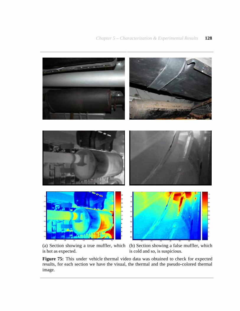
Chapter 5 – Characterization & Experimental Results 128
(a) Section showing a true muffler, which is hot as expected.
(b) Section showing a false muffler, which is cold and so, is suspicious.
Figure 75: This under vehicle thermal video data was obtained to check for expected results, for each section we have the visual, the thermal and the pseudo-colored thermal image.
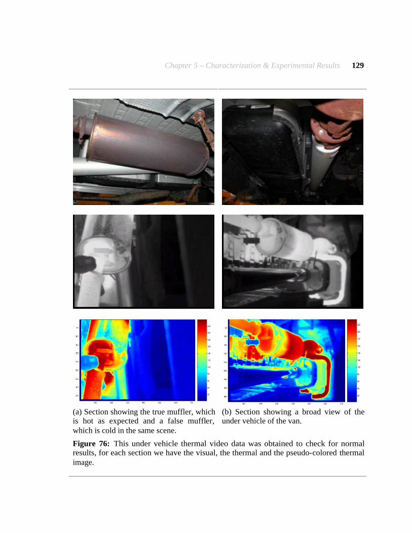
Chapter 5 – Characterization & Experimental Results 129
(a) Section showing the true muffler, which is hot as expected and a false muffler, which is cold in the same scene.
(b) Section showing a broad view of the under vehicle of the van.
Figure 76: This under vehicle thermal video data was obtained to check for normal results, for each section we have the visual, the thermal and the pseudo-colored thermal image.
Chapter 5 – Characterization & Experimental Results 130
5.2.3 Under vehicle thermal video sequences (Threat detection)
As part of this experiment we acquired thermal data for under vehicle threat detection. Figure 77 below shows images of the Ford Taurus car, Dodge Stratus car and Dodge RAM 3500 van used for threat detection experiments in under vehicle surveillance. The TISB system was mounted on the SafeBot under vehicle robot for inspection and was controlled remotely (wirelessly) by the user as seen in Figure 77. We randomly planted a self-designed threat object at different locations in the undercarriage of the vehicle and tested the ability of the thermal sensor brick in highlighting its presence. Figure 78, Figure 79 and Figure 80 below, each show us a different view of the under carriage of the Ford Taurus car with and without the threat object, for each view we have a visual image, a thermal image and a pseudo-colored thermal image. As we can see from these images, we can barely notice the presence of the hidden threat object in the visual image but it stands out in the thermal images. The same process was repeated for the Dodge RAM 3500 van, wherein we planted a threat object underneath the vehicle and tested if the sensor brick could detect it. Figure 81, Figure 82, Figure 83, Figure 84 and Figure 85 below, each show us a different view of the undercarriage of the Dodge RAM 3500 van with and without the threat object. Once again we can see that we can hardly tell the presence of the threat object in the visual images but the difference is distinct in the thermal images.
5.2.4 Complete under vehicle thermal video sequences
As part of this experiment we acquired thermal data for complete under vehicle surveillance. Mounting the TISB system on the SafeBot under vehicle robot and navigating it manually we acquired this data. The robot can also navigate autonomously. This data was collected so that it can be used in the future to generate a thermal mosaic of the undercarriage of a car / van. We collected two sets of data for each vehicle. One set was obtained with the robot moving from the rear to the front and the other vice-versa. The data was obtained in strips 1’ 3” wide, starting from the left of the vehicle and moving to the right from the rear to the front and vice-versa. For each strip the robot traversed a straight-line path under the vehicle. There was about 15% - 25% overlap between successive strips. All the datasets were collected along the length of the vehicle. Figure 86 below shows the diagrammatic representation of the floor dimensions for the Dodge RAM 3500 van and the Dodge Stratus car and the methodology used in data acquisition. The floor dimensions of the Dodge RAM 3500 van and the Dodge Stratus car are as given in Table 20 below.

Chapter 5 – Characterization & Experimental Results 131
(a) (b)
(c) (d)
Figure 77: (a), (b), (c) and (d) are different images of the Ford Taurus car, Dodge Stratus car and Dodge RAM 3500 van used for threat detection experiments in under vehicle surveillance. We can see the sensor brick mounted on the SafeBot under vehicle robot for inspection and is remotely (wirelessly) controlled by the user.
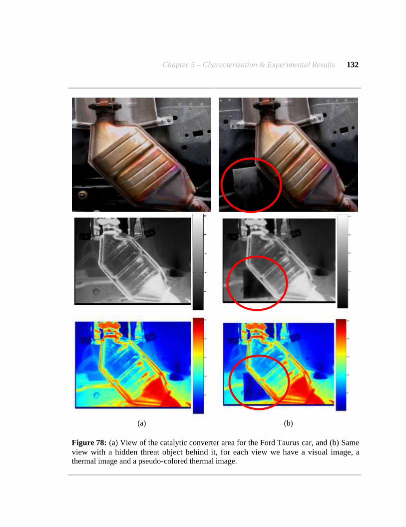
Chapter 5 – Characterization & Experimental Results 132
(a) (b)
Figure 78: (a) View of the catalytic converter area for the Ford Taurus car, and (b) Same view with a hidden threat object behind it, for each view we have a visual image, a thermal image and a pseudo-colored thermal image.

Chapter 5 – Characterization & Experimental Results 133
(a) (b)
Figure 79: (a) View of the gas tank area for the Ford Taurus car, and (b) Same view with a hidden threat object behind it, for each view we have a visual image, a thermal image and a pseudo-colored thermal image.
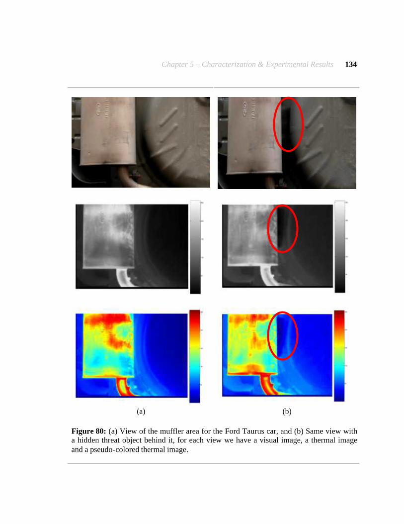
Chapter 5 – Characterization & Experimental Results 134
(a) (b)
Figure 80: (a) View of the muffler area for the Ford Taurus car, and (b) Same view with a hidden threat object behind it, for each view we have a visual image, a thermal image and a pseudo-colored thermal image.
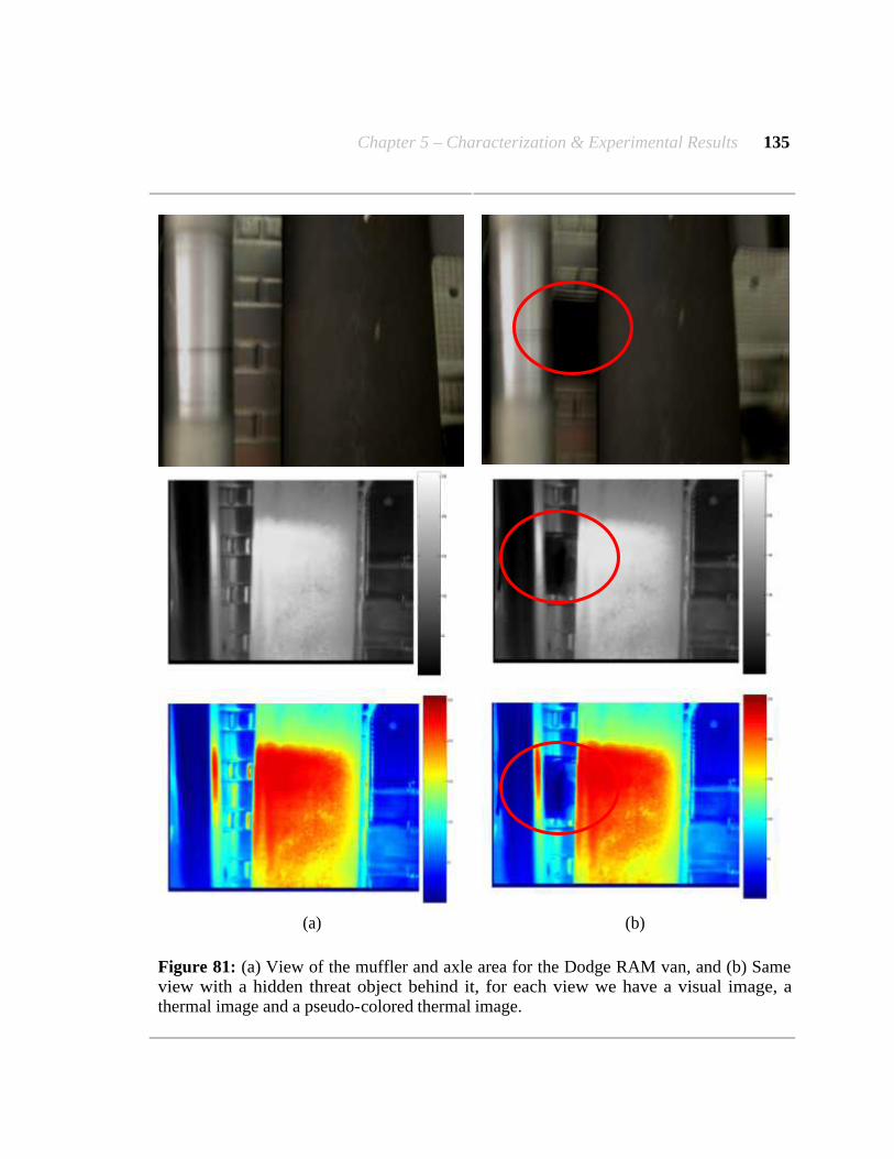
Chapter 5 – Characterization & Experimental Results 135
(a) (b)
Figure 81: (a) View of the muffler and axle area for the Dodge RAM van, and (b) Same view with a hidden threat object behind it, for each view we have a visual image, a thermal image and a pseudo-colored thermal image.

Chapter 5 – Characterization & Experimental Results 136
(a) (b)
Figure 82: (a) View of the exhaust manifold area for the Dodge RAM van, and (b) Same view with a hidden threat object behind it, for each view we have a visual image, a thermal image and a pseudo-colored thermal image.
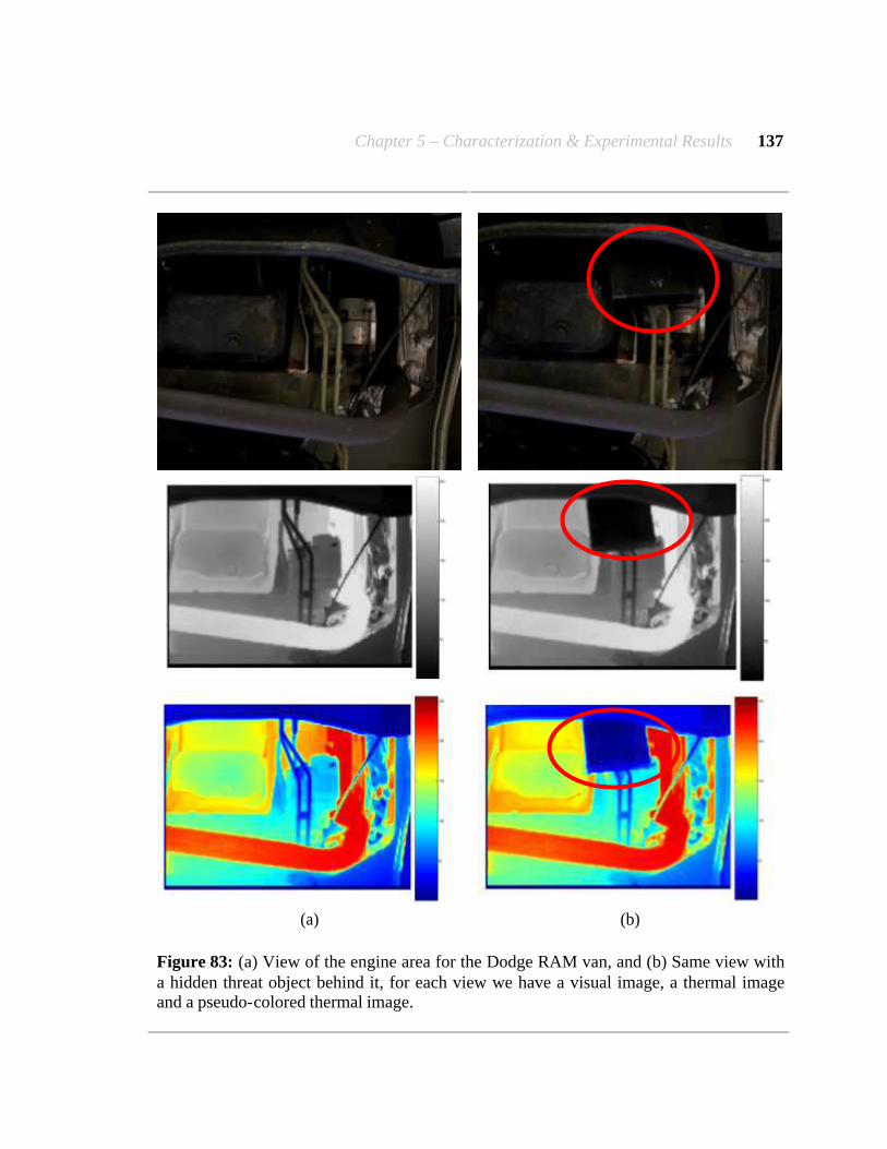
Chapter 5 – Characterization & Experimental Results 137
(a) (b)
Figure 83: (a) View of the engine area for the Dodge RAM van, and (b) Same view with a hidden threat object behind it, for each view we have a visual image, a thermal image and a pseudo-colored thermal image.

Chapter 5 – Characterization & Experimental Results 138
(a) (b)
Figure 84: (a) View of the gas tank and axle area for the Dodge RAM van, and (b) Same view with a hidden threat object behind it, for each view we have a visual image, a thermal image and a pseudo-colored thermal image.

Chapter 5 – Characterization & Experimental Results 139
(a) (b)
Figure 85: (a) View of an area at the rear end of the Dodge RAM van, and (b) Same view with a hidden threat object behind it, for each view we have a visual image, a thermal image and a pseudo-colored thermal image.

Chapter 5 – Characterization & Experimental Results 140
Table 20: Floor dimensions for the Dodge RAM van and the Dodge Stratus car used for thermal imaging in complete under vehicle surveillance.
Dodge RAM 3500 van. Length of the van: 19’ 8”. Width of the van: 6’4”.
Distance between wheel bases along the axle: 4’8”. Distance between center’s of the wheel’s: 10’7”
Wheel radius: 1’4”. Dodge Stratus car.
Length of the car: 16’0”. Width of the car: 5’7”.
Distance between wheel bases along the axle: 4’4”. Distance between center’s of the wheel’s: 9’1”.
Wheel radius: 1’0”.
Figure 86: Diagrammatic representation of the floor dimensions of the Dodge RAM 3500 van and Dodge Stratus car used for thermal imaging in complete under vehicle surveillance video sequences.
Chapter 6 – Conclusions 141
6 Conclusions
6.1 Summary
This research has successfully demonstrated the design, development and characterization of the TISB system, which is based on the design philosophy of sensor bricks for modular robotics. We have highlighted the advantages of the TISB system over purely vision-based systems in under vehicle surveillance for threat detection, which is a target application of our work. We have also demonstrated the capability of the system to be operational when fitted on the SafeBot under vehicle robot and acquired data using it. We have also looked at the evolution of the designs and the uniformity achieved by us while maintaining modularity in building the different sensor bricks namely the visual, the thermal and the range sensor brick.
6.2 Contributions
The contributions of this thesis are: · Designing and developing the hardware implementation of the TISB system.
· Designing and developing the software for the TISB system. · Characterizing the TISB system, where this characterization of the system is the
major contribution of this thesis.
6.3 Lessons Learned
Based on our literature review and our experimentation we can conclude that modular sensor bricks are one of the means to address the problem of designing, fabricating and testing cost-effective intelligent mobile robotic systems. Some of the advantages of modular systems other than being highly modular are they are completely self-sufficient, not built for specific applications, small in size, light in weight, like plug and play devices (no external connections required) which enhances easy swapping out between different sensor bricks and cost effective since they use COTS technology. The design of modular systems provides for easy component replacement due to damage or technological upgrade. All these advantages aid in improving the operational reliability and effectiveness of mobile robotic systems. The TISB system, which we have dealt with in detail has been proven to be an illumination invariant threat detection system for detecting hidden threat objects in the undercarriage of a car as compared to the vision sensor brick system and the mirror on a stick.

Chapter 6 – Conclusions 142
6.4 Future Work
The analysis of the TISB system provides with sufficient information on parameters to be considered to make the right choice for future modifications. For applications where accurate prediction of scene temperature based on the image is necessary we would have to use a calibrated thermal camera. The current system processor is capable of handling all its requirements but advancement in technology could prompt a change in the chip. Wireless communications standard could be upgraded with advancement in technology to enhance data handling capabilities and range of operation of the system. The batteries that are currently being used on the system meet its power needs for up to 5.0 hours of operation, smaller and more efficient batteries could be looked into. Also as part of the future work we could improve the current algorithms for change detection and counting people and make them to be completely autonomous and more reliable. Specific software packages could be developed for individual target applications of under vehicle surveillance for threat detection, perimeter / area surveillance, scouting, and IED detection using a car-mounted system. The task of integration of data from different sensor brick systems could be looked into. We could develop a GUI to control SafeBot – B, which can carry all the four sensor bricks at same instance and this GUI would display the data available from all the four different sensors at the same time. Using this GUI we could be able to control the robot and the bricks.

References 143
References

References 144
[1] J. Kostrzewa, W. Meyer, W. Terre, S. Laband and G. W. Newsome, “Use of a Miniature Infrared COTS Sensor in Several Military Applications,” in Proc. SPIE Unattended Ground Sensor Technologies and Applications IV, Vol. 4743, Orlando, FL, USA, pp. 141-149, August 2002. [2] J. Kostrzewa, W. Meyer, D. Kraemer, G. Poe, V. Nguyen, M. Brown, W. Terre, G. Newsome, “Overview of The UL3 Omega Uncooled Camera and its Applications,” in Proc. SPIE Infrared and Passive Millimeter-wave Imaging Systems: Design Analysis, Modeling and Testing, Vol. 4719, Orlando, FL, USA, pp. 189-195, July 2002. [3] S. Katwal, “Range Sensor Brick for Modular Robotics,” Project In-Lieu Of Thesis (PILOT) Report, University of Tennessee, Knoxville, TN, USA, December 2004. [4] A Poduri, “Video Sensor Brick for Modular Robotics,” Project In-Lieu Of Thesis (PILOT) Report, University of Tennessee, Knoxville, TN, USA, December 2004. [5] B. Ramadoss, “Hardware and Software Development of a Wireless Imaging System for Under Vehicle Inspection Robot,” Project In-Lieu Of Thesis (PILOT) Report, University of Tennessee, Knoxville, TN, USA, December 2003. [6] Tom Wilson, “A Comparison of the Sensor Brick Concept as a Modular System Architecture to the Realtime Control System as the Operational Architecture,” M.S. Thesis, University of Tennessee, Knoxville, TN, USA, December 2005. [7] Yue Zheng, “X - Ray Image Processing and Visualization for Remote Assistance of Airport Luggage Scanners,” M.S. Thesis, University of Tennessee, Knoxville, TN, USA, December 2004. [8] Omega Camera User’s Guide, Indigo Systems Corporation, Goleta, CA, 2003. [9] D. Page, Y. Fougerolle, A. Koschan, A. Gribok, M. Abidi, D. Gorsich, and G. Gerhart, “SAFER Vehicle Inspection: A Multimodal Robotic Sensing Platform”, in Proc. SPIE Unmanned Ground Vehicle Technology VI, Vol. 5422, Orlando, FL, USA, pp. 549-560, April 2004. [10] C. Qian, D. Page, A. Koschan and M. Abidi, “A “Brick”-Architecture-Based Mobile Under-Vehicle Inspection System”, in Proc. SPIE Unmanned Ground Vehicle Technology VII, Vol. 5804, Orlando, FL, USA, pp. 182-190, March 2005. [11] K. L. Moore, N. S. Flann, S. C. Rich, M Frandsen, Y. C. Chung, J. Martin, M. E. Davidson, R. Maxfield and C. Wood, “Implementation of an Omni Directional Robotic Inspection System (ODIS),” in Proc. SPIE Unmanned Ground Vehicle
References 145
Technology III, Vol. 4364, Orlando, FL, USA, pp. 200-210, September 2001. [12] B. Smuda, E. Schoenherr, H. Andrusz, G. Gerhart, “Deploying the ODIS Robot in Iraq and Afghanistan,” in Proc. SPIE Unmanned Ground Vehicle Technology VII, Vol. 5804, Orlando, FL, USA, pp. 119-129, May 2005. [13] W. Smuda, P. L. Muench, G. R. Gerhart, “Autonomy and Manual Operation in a Small Robotic System for Under-Vehicle Inspections at Security Checkpoints,” in Proc. SPIE Unmanned Ground Vehicle Technology IV, Vol. 4715, Orlando, FL, USA, pp. 1-12, July 2002. [14] J. S. Albus, A. M. Meystel. Engineering of mind: An Introduction to the Science of Intelligent Systems. New York: John Wiley and Sons, 2001. [15] R. Murphy. Introduction to AI Robotics. Cambridge, Mass.: The MIT Press, 2000. [16] R. Arkin. Behavior-based Robotics. Cambridge, Mass.: The MIT Press, 1998. [17] JAUS Working Group, “Joint Architecture for Unmanned Systems (JAUS): Reference Architecture Specification”, Version 3.0, Volume 2, 2002. Joint Architecture for Unmanned Systems, http://www.jauswg.org [18] R. C. Gonzalez, W. E. Woods. Digital Image Processing 2ndEdition. Upper Saddle River NJ: Prentice Hall, 2002. [19] J. M. Lloyd. Thermal Imaging Systems. New York: Plenum Press, 1975. [20] W. S. Janna. Engineering Heat Transfer. Boca Raton, FL.: CRC Press, 2000. [21] FLIR Systems Core by Indigo, Omega thermal cameras, Santa Barbara, CA, http://www.indigosystems.com/products/core_micron.html. [22] iBT Technologies Inc., IBASE series of computer motherboards, Canada, http://www.ibt.ca/IB880.htm. [23] INTEL Corporation, Hardware developer, USA, http://www.intel.com. [24] HyperLink Technologies Inc., Rubber duck antennas, Boca Raton, FL, http://www.hyperlinktech.com/web/hg2405rd_rsp.php. [25] Power Factor Inc., Panasonic batteries, Dallas, TX, http://www.powerfactorinc.com/Batteries/lc-ra1212p.htm.

References 146
[26] Vicor Corporation, DC-to-DC converters, Andover, MA, http://www.vicr.com. [27] OPUS Solutions Inc., ATX power supplies, Laguna Hills, CA, http://www.opussolutions.com. [28] Astrodyne International, AC-to-DC rectifiers, Taunton, MA, http://www.astrodyne.com/astro/default.asp. [29] Euresys Inc., Picolo series of video capture card, Itasca, IL, http://www.euresys.com. [30] A seminar presentation on the applications of infrared imaging, “Teamworknet Inc website”, http://www.teamworknet.com/ResourceLibrary/Presentations/IEEEThermalPresentation/default.asp#1. [31] Australian Thermal Imaging Pvt Ltd, Australia, http://www.thermalimaging.com.au. [32] The Law Enforcement Thermographers Association (LETA), http://www.leta.org. [33] Remotec a subsidiary of Northrop Grumman, Andros Family of tracked vehicles, Oak Ridge, TN, http://www.es.northropgrumman.com/remotec/about_remotec.htm. [34] Foster-Miller Inc., Talon family of tracked vehicles, Waltham, MA, http://www.foster-miller.com. [35] iRobot Corporation, Talon family of tracked vehicles, Burlington, MA, http://www.irobot.com. [36] Autonomous Solutions Inc, Spector Omni-Directional Under vehicle Inspection System, Young Ward, UT, http://www.autonomoussolutions.com/Products/Spector/index.html [37] K. Moore, G. Gerhart, “The TACOM-USU Intelligent Mobility Program,” in Proc. SPIE Unmanned Ground Vehicle Technology VI, Vol. 5422, Orlando, FL, USA, pp. 258-269, April 2004.
References 147
[38] C, Bererton, L. Navarro-Serment, R. Grabowski, C. Paredis and P. Khosla, “Millibots: Small Distributed Robots for Surveillance and Mapping,” Government Microcircuit Applications Conference, March 2000. [39] Wintron Technologies, Under Vehicle Inspection Systems, http://www.wintrontech.com/security/index.html. [40] Search Systems Inc, Under Vehicle Inspection System, Bakersfield, CA http://www.searchsystems.com/contraband_uvis.html. [41] Lumenyte International Corporation, Under Vehicle Inspection Systems, Foothill Ranch, CA http://www.lumenyte.com/product/HomelandSecurity/homesec.htm. [42] Northrop Grumman, Under Vehicle Inspection System (UVIS), McLean, VA, http://www.it.northropgrumman.com/MMPDFs/UVIS.pdf. [43] Prolite Armor Systems, Under Vehicle Inspection System (UVIS), Amityville, NY http://www.publicsafetymall.com/UVIS.htm. [44] Vehicle Inspection Technologies (VIT), Und- Aware Under Vehicle Inspection and Surveillance System, Sterling VA, http://www.undaware.com/default.asp. [45] Wolstenholme Machine Inc, Under Vehicle Surveillance Systems, Colmar, PA, http://www.wmrobots.com/undervehicle.php. [46] Computer Vision Laboratory, University of Massachusetts Amherst, Under Vehicle Inspection System (UVIS) http://vis-www.cs.umass.edu/projects/uvis/start.html. [47] Gatekeeper Security, Vehicle Undercarriage Inspection Ramp, Reston, VA, http://www.gatekeepersecurity.com/products/undercarriage_inspection.php. [48] R. Bodor, B. Jackson, N Papanikolopoulos, “Vision-Based Human Tracking and Activity Recognition,” in Proc. 11th Mediterranean Conference on Control and Automation, June 2003. [49] U. M. Braga-Neto, M. Choudhary, J. Goutsias, “Automatic Target Detection and Tracking on Forward-Looking Infrared Image Sequences Using Morphological Connected Operators,” Journal of Electronic Imaging, 13(4), pp. 802-813, April 2004.
References 148
[50] C. Eveland, D. Socolinsky, L. Wolff, “Tracking Human Faces in Infrared Video,” Journal of Image and Vision Computing, 21(7), pp. 579-590, July 2003. [51] Y. Fang, I. Masaki, B. Horn, “A New Night Visionary Pedestrian Detection and Warning Systems,” Artificial Intelligence Laboratory, MIT, Cambridge, MA. [52] S. Feller, E. Cull, D. Kowalski, K. Farlow, J. Burchett, J. Adleman, C. Lin, D. Brady, “Tracking and Imaging Humans on Heterogeneous Infrared Sensor Array for Tactical Applications,” in Proc. SPIE Unattended Ground Sensor Technologies and Applications IV, Vol. 4743, Orlando, FL, USA, pp. 168-175, August 2002. [53] I. Haritaoglu, D. Harwood, L. Davis, “W4 : Who? When? Where? What? A Real Time System for Detecting and Tracking People,” in Proc. 3rd International Conference on Face and Gesture Recognition, Nara, Japan, pp. 222-227, April 1998. [54] I. Haritaoglu, D. Harwood, L. Davis, “Ghost: A Human Body Part Labeling System Using Silhouettes,” in Proc. 14th International Conference on Pattern Recognition, Brisbane, Australia, pp. 77-82, August 1998. [55] B. Maurin, O. Masoud, N. Papanikolopoulos, “Monitoring crowded traffic scenes,” Proc. IEEE 5th International Conference on Intelligent Transportation Systems (ITSC 2002), Singapore, pp. 19-24, September 2002. [56] M. Nakamura, H. Zhao, R. Shibasaki, “Tracking passenger movement with infrared video data,” in Proc. ACRS 2001-22nd Asian Conference on Remote Sensing, Vol. 2, Singapore, pp. 1520-1523, November 2001. [57] H. Nanda, L. Davis, “Probabilistic Template Based Pedestrian Detection in Infrared Videos,” Proc. IEEE Intelligent Vehicle Symposium, Versailles, France, June 2002. [58] F. Xu, K. Fujimara, “Pedestrian Detection and Tracking with Night Vision,” in Proc. IEEE Intelligent Vehicles Symposium, Versailles, France, June 2002. [59] Palo Alto Research Center, Modular Robotics Project, Palo Alto, CA, http://www2.parc.com/spl/projects/modrobots.

Appendices 149
Appendices
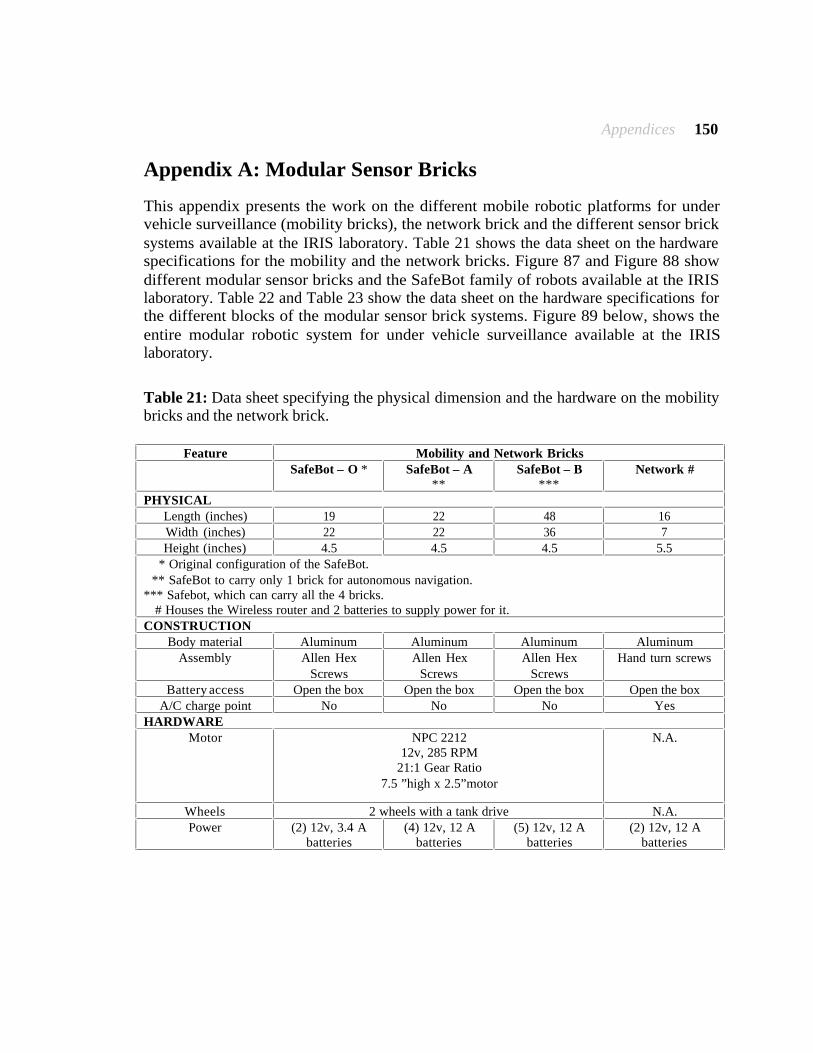
Appendices 150
Appendix A: Modular Sensor Bricks
This appendix presents the work on the different mobile robotic platforms for under vehicle surveillance (mobility bricks), the network brick and the different sensor brick systems available at the IRIS laboratory. Table 21 shows the data sheet on the hardware specifications for the mobility and the network bricks. Figure 87 and Figure 88 show different modular sensor bricks and the SafeBot family of robots available at the IRIS laboratory. Table 22 and Table 23 show the data sheet on the hardware specifications for the different blocks of the modular sensor brick systems. Figure 89 below, shows the entire modular robotic system for under vehicle surveillance available at the IRIS laboratory.
Table 21: Data sheet specifying the physical dimension and the hardware on the mobility bricks and the network brick.
Feature Mobility and Network Bricks SafeBot – O *
SafeBot – A
** SafeBot – B
*** Network #
PHYSICAL
Length (inches) 19 22 48 16 Width (inches) 22 22 36 7 Height (inches) 4.5 4.5 4.5 5.5
* Original configuration of the SafeBot. ** SafeBot to carry only 1 brick for autonomous navigation. *** Safebot, which can carry all the 4 bricks. # Houses the Wireless router and 2 batteries to supply power for it. CONSTRUCTION
Body material Aluminum Aluminum Aluminum Aluminum Assembly Allen Hex
Screws Allen Hex
Screws Allen Hex
Screws Hand turn screws
Battery access Open the box Open the box Open the box Open the box A/C charge point No No No Yes
HARDWARE Motor NPC 2212
12v, 285 RPM 21:1 Gear Ratio
7.5 ”high x 2.5”motor
N.A.
Wheels 2 wheels with a tank drive N.A. Power (2) 12v, 3.4 A
batteries (4) 12v, 12 A
batteries (5) 12v, 12 A
batteries (2) 12v, 12 A
batteries

Appendices 151
(a) (b)
(c) (d)
(e) (f)
Figure 87: Images of Range Sensor Brick, Thermal Sensor Brick and Visual Sensor Brick that have been implemented at the IRIS laboratory.
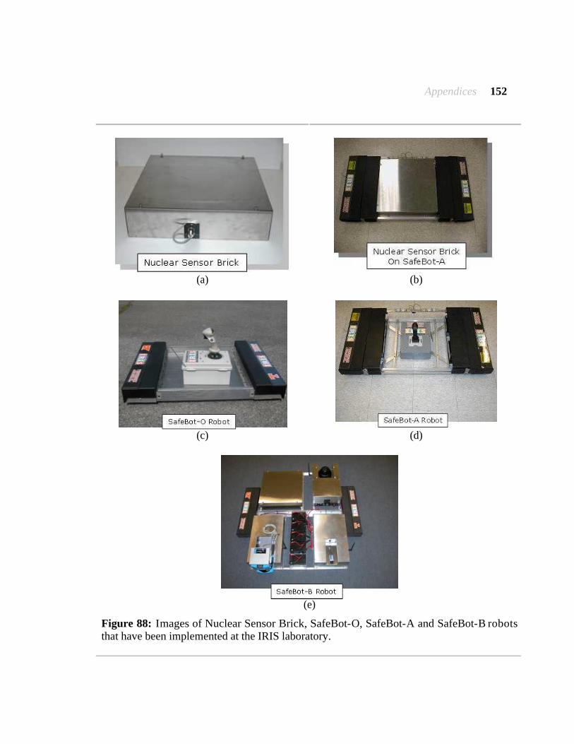
Appendices 152
(a) (b)
(c) (d)
(e)
Figure 88: Images of Nuclear Sensor Brick, SafeBot-O, SafeBot-A and SafeBot-B robots that have been implemented at the IRIS laboratory.
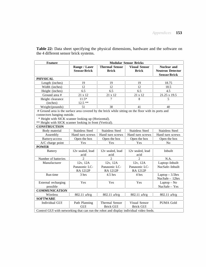
Appendices 153
Table 22: Data sheet specifying the physical dimensions, hardware and the software on the 4 different sensor brick systems.
Feature Modular Sensor Bricks Range / Laser
Sensor Brick Thermal Sensor
Brick Visual Sensor
Brick Nuclear and
Neutron Detector Sensor Brick
PHYSICAL Length (inches) 19 19 19 18.75 Width (inches) 12 12 12 18.5 Height (inches) 6.5 6.5 6.5 4.5 Ground area # 21 x 12 21 x 12 21 x 12 21.25 x 19.5
Height clearance (inches)
11.5* 12.5 **
7 8 5
Weight (pounds) 51 38 41 40 # Ground area is the surface area covered by the brick while sitting on the floor with its ports and connectors hanging outside. * Height with SICK scanner looking up (Horizontal). ** Height with SICK scanner looking in front (Vertical). CONSTRUCTION
Body material Stainless Steel Stainless Steel Stainless Steel Stainless Steel Assembly Hand turn screws Hand turn screws Hand turn screws Hand turn screws
Battery access Open the box Open the box Open the box Open the box A/C charge point Yes Yes Yes No
POWER Battery 12v sealed, lead
acid 12v sealed, lead
acid 12v sealed, lead
acid Inbuilt
Number of batteries 2 2 2 N.A. Manufacturer 12v, 12A
Panasonic LC-RA 1212P
12v, 12A Panasonic LC-
RA 1212P
12v, 12A Panasonic LC-
RA 1212P
Laptop–Inbuilt NucSafe–Inbuilt
Run time 3 hrs 4.5 hrs 4 hrs Laptop – 3.5hrs NucSafe – 12hrs
External recharging possible
Yes Yes Yes Laptop – No NucSafe – Yes
COMMUNICATION Wireless 802.11 a/b/g 802.11 a/b/g 802.11 a/b/g 802.11 a/b/g
SOFTWARE Individual GUI Path Planning
GUI Thermal Sensor
Brick GUI Visual Sensor
Brick GUI PUMA Gold
Control GUI with networking that can run the robot and display individual video feeds.
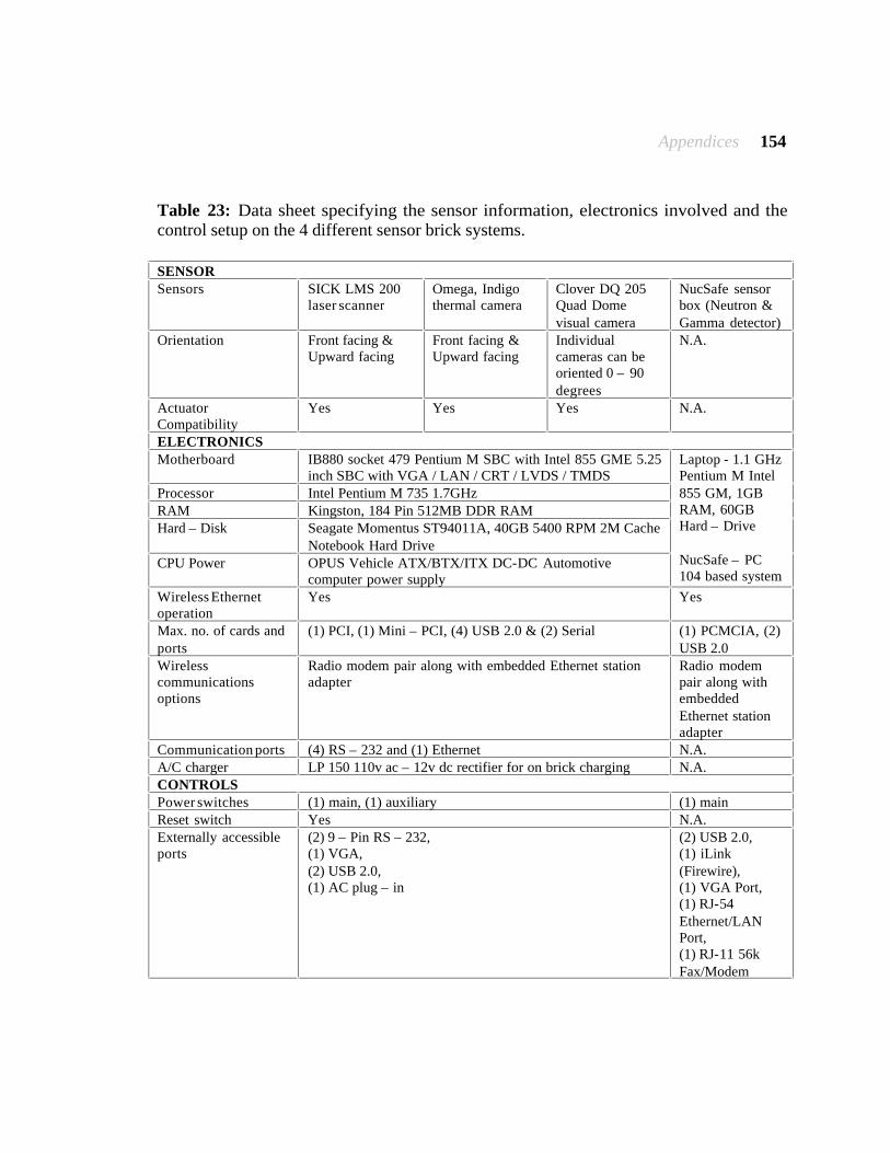
Appendices 154
Table 23: Data sheet specifying the sensor information, electronics involved and the control setup on the 4 different sensor brick systems. SENSOR Sensors SICK LMS 200
laser scanner Omega, Indigo thermal camera
Clover DQ 205 Quad Dome visual camera
NucSafe sensor box (Neutron & Gamma detector)
Orientation Front facing & Upward facing
Front facing & Upward facing
Individual cameras can be oriented 0 – 90 degrees
N.A.
Actuator Compatibility
Yes Yes Yes N.A.
ELECTRONICS Motherboard IB880 socket 479 Pentium M SBC with Intel 855 GME 5.25
inch SBC with VGA / LAN / CRT / LVDS / TMDS Processor Intel Pentium M 735 1.7GHz RAM Kingston, 184 Pin 512MB DDR RAM Hard – Disk Seagate Momentus ST94011A, 40GB 5400 RPM 2M Cache
Notebook Hard Drive CPU Power OPUS Vehicle ATX/BTX/ITX DC-DC Automotive
computer power supply
Laptop - 1.1 GHz Pentium M Intel 855 GM, 1GB RAM, 60GB Hard – Drive NucSafe – PC 104 based system
Wireless Ethernet operation
Yes Yes
Max. no. of cards and ports
(1) PCI, (1) Mini – PCI, (4) USB 2.0 & (2) Serial (1) PCMCIA, (2) USB 2.0
Wireless communications options
Radio modem pair along with embedded Ethernet station adapter
Radio modem pair along with embedded Ethernet station adapter
Communication ports (4) RS – 232 and (1) Ethernet N.A. A/C charger LP 150 110v ac – 12v dc rectifier for on brick charging N.A. CONTROLS Power switches (1) main, (1) auxiliary (1) main Reset switch Yes N.A. Externally accessible ports
(2) 9 – Pin RS – 232, (1) VGA, (2) USB 2.0, (1) AC plug – in
(2) USB 2.0, (1) iLink (Firewire), (1) VGA Port, (1) RJ-54 Ethernet/LAN Port, (1) RJ-11 56k Fax/Modem
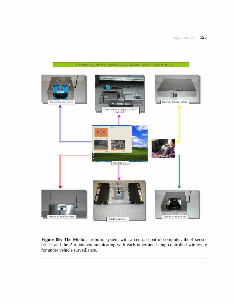
Appendices 155
Figure 89: The Modular robotic system with a central control computer, the 4 sensor bricks and the 2 robots communicating with each other and being controlled wirelessly for under vehicle surveillance.

Vita 156
Vita
Nikhil Arun Naik was born in Panaji, Goa, India on December 5, 1980, to Mrs. Rati A. Naik and Mr. Arun B. Naik. He received his Bachelor of Engineering degree in Electronics and Telecommunications Engineering in July 2002, from The Padre Conceicao College of Engineering, Goa University; Goa, India. He joined The University of Tennessee, Knoxville in fall 2003 as a graduate student in Electrical and Computer Engineering and accepted a position with The Imaging, Robotics and Intelligence Systems (IRIS) laboratory as a graduate research assistant in spring 2004. He completed his requirements for the Master of Science degree in summer 2006. In the future, he would like to learn how to fly an airplane; his passion is cricket, soccer and fast cars. If he were not to be an engineer he would have been a professional cricket player.