
To Sell and to Provide? The Economic and …bt71/articles/BFT2016.pdf · The Economic and...
38
To Sell and to Provide? The Economic and Environmental Implications of the Auto Manufacturer’s Involvement in the Car Sharing Business Ioannis Bellos School of Business, George Mason University, Fairfax, VA 22030, [email protected] Mark Ferguson Moore School of Business, University of South Carolina, Columbia, SC 29208, [email protected] L. Beril Toktay Scheller College of Business, Georgia Institute of Technology, Atlanta, GA 30308, [email protected] Motivated by the involvement of Daimler and BMW in the car sharing business we consider an OEM who contemplates introducing a car sharing program. The OEM designs its product line by accounting for the trade-off between driving performance and fuel efficiency. Customers have different valuations of driving performance and decide whether to buy, join car sharing, or rely on their outside option. Car sharing can increase the profit from selling. This happens when the OEM prefers to serve the lower-end customers through car sharing and the higher-end through selling. In this case, car sharing increases the efficiency of the vehicles used for the lower-end, and the price charged to the higher-end customers. This is more pronounced for higher-end OEMs, which may help explain Daimler’s and BMW’s involvement in car sharing. Despite the higher efficiency, car sharing may lower the OEM’s Corporate Average Fuel Economy (CAFE) level even when it increases profit and decreases environmental impact. CAFE levels better reflect the environmental benefits of car sharing when they are based on the number of customers served and not the production volume. Finally, if anticipating aggressive CAFE standards, OEMs may include car sharing to better absorb the increase in the production cost. Key words : car sharing; sustainable transportation; sustainable business models; CAFE standards; fuel efficiency; product line 1. Introduction In recent years, car sharing has been increasingly seen as a viable alternative to car own- ership. Under a typical car sharing model, after paying a yearly fee, customers become members of the car sharing program and obtain access to a fleet of vehicles that they can use in increments as short as one hour. Members are charged based on the duration of the time they remove a vehicle from the service pool while gas, maintenance, and insur- ance are included in the hourly price. In this manner, car sharing transforms the fixed 1
-
Upload
duongthien -
Category
Documents
-
view
218 -
download
0
Transcript of To Sell and to Provide? The Economic and …bt71/articles/BFT2016.pdf · The Economic and...
To Sell and to Provide?The Economic and Environmental Implications of theAuto Manufacturer’s Involvement in the Car Sharing
Business
Ioannis BellosSchool of Business, George Mason University, Fairfax, VA 22030, [email protected]
Mark FergusonMoore School of Business, University of South Carolina, Columbia, SC 29208, [email protected]
L. Beril ToktayScheller College of Business, Georgia Institute of Technology, Atlanta, GA 30308, [email protected]
Motivated by the involvement of Daimler and BMW in the car sharing business we consider an OEM who
contemplates introducing a car sharing program. The OEM designs its product line by accounting for the
trade-off between driving performance and fuel efficiency. Customers have different valuations of driving
performance and decide whether to buy, join car sharing, or rely on their outside option. Car sharing can
increase the profit from selling. This happens when the OEM prefers to serve the lower-end customers
through car sharing and the higher-end through selling. In this case, car sharing increases the efficiency of the
vehicles used for the lower-end, and the price charged to the higher-end customers. This is more pronounced
for higher-end OEMs, which may help explain Daimler’s and BMW’s involvement in car sharing. Despite
the higher efficiency, car sharing may lower the OEM’s Corporate Average Fuel Economy (CAFE) level even
when it increases profit and decreases environmental impact. CAFE levels better reflect the environmental
benefits of car sharing when they are based on the number of customers served and not the production
volume. Finally, if anticipating aggressive CAFE standards, OEMs may include car sharing to better absorb
the increase in the production cost.
Key words : car sharing; sustainable transportation; sustainable business models; CAFE standards; fuel
efficiency; product line
1. Introduction
In recent years, car sharing has been increasingly seen as a viable alternative to car own-
ership. Under a typical car sharing model, after paying a yearly fee, customers become
members of the car sharing program and obtain access to a fleet of vehicles that they can
use in increments as short as one hour. Members are charged based on the duration of
the time they remove a vehicle from the service pool while gas, maintenance, and insur-
ance are included in the hourly price. In this manner, car sharing transforms the fixed
1

Bellos, Ferguson, and Toktay:2 To Sell and to Provide?
costs associated with the ownership of a vehicle (e.g., purchase cost, depreciation, insur-
ance) to a variable cost that depends on vehicle usage. Zipcar, founded in 1999, is the
largest for-profit car sharing provider with over 900,000 members across the U.S., Canada,
and Europe (Zipcar 2016b). According to Shaheen and Cohen (2015) the number of car
sharing members in the U.S. has increased from 52K in 2004 to 1.28M in 2015. Navigant
Research (2013) estimates that by 2020 the global car sharing market will be worth $6.2B
in revenues.
Although car sharing programs are typically associated with independent providers
like Zipcar, several auto manufacturers have recently started introducing car sharing
schemes. Daimler, for example, operates a car sharing program in several cities in the U.S.
and Europe (CAR2GO 2016), while BMW operated a similar scheme in San Francisco
(DriveNow 2015) with the city of Seattle to follow soon (The Seattle Times 2015). In addi-
tion, Peugeot, Volkswagen, and Ford operate car sharing programs in several European
cities (Mu 2016, Quicar 2016, Ford 2015). Recently, GM started testing its own car shar-
ing program in the city of Ann Arbor (The Wall Street Journal 2016). Such moves are
indicative of a broader transformation that auto manufacturers are undergoing to become
mobility companies (Fortune 2015).
Nevertheless, the economic benefits of the auto manufacturers’ strategy of introducing
car sharing programs are not clear. On the one hand, offering products under membership-
based schemes may cannibalize the demand from customers who otherwise would purchase
vehicles and, therefore, may decrease the manufacturers’ profitability. For example, Zipcar
estimates that in the absence of car sharing, one out of four of their members would have
bought a car (Zipcar 2016a). On the other hand, car sharing can benefit the auto manufac-
turers (henceforth “OEMs”) by potentially expanding the customer base to segments that
previously did not own a car. For instance, a car sharing scheme may appear attractive to
commuters who normally use alternative transportation modes such as public transporta-
tion. Even in the absence of such a market expansion effect, OEMs may benefit from a
decrease in their total production cost through a pooling effect as, under car sharing, the
same vehicle can be used by many customers at different periods of time, resulting in a
lower production volume.
In addition to the increasing interest of manufacturers in providing car sharing programs,
the U.S. Environmental Protection Agency has categorized car sharing as a top-ten, high-
potential “green” business model (U.S. EPA 2009). Along these lines, car sharing providers
Bellos, Ferguson, and Toktay:To Sell and to Provide? 3
often promote their programs by highlighting their environmental superiority over the more
conventional practice of selling cars. For instance, Zipcar claims that each shared car covers
the transportation needs of 40 members (Zipcar 2016a). Navigant Research (2013) also
estimates that each shared car takes approximately 5 to 11 vehicles off the road (Shaheen
and Cohen 2015 estimate this to be 9 to 13 vehicles). On the negative side, however, by
reaching out to customers who previously did not own a vehicle and enabling them to start
using one, car sharing can increase the overall environmental impact of transportation.
Improving environmental performance may be particularly important to OEMs because
of the evolving environmental regulations around emission standards. Specifically, auto-
motive industry OEMs are required to comply with the Corporate Average Fuel Economy
(CAFE) standards set by the U.S. Department of Transportation. Although this regula-
tion has been in effect since 1975, the standards are scheduled to increase rapidly over the
next few years with the target for 2025 set at 54.51 miles per gallon (U.S. Department of
Transportation 2012). Surveying the average fleet efficiency of different OEMs reveals that
BMW and Daimler, along with other “high-end” OEMs like Jaguar and Volvo, have been
among the least fuel-efficient manufacturers (see summary prepared by the NHTSA 2014).
Interestingly, Daimler and BMW have also been among the first manufacturers to actively
engage in the car sharing business.
The objective of the CAFE regulation is to incentivize OEMs to improve the fuel effi-
ciency of their vehicles. Besides the obvious cost implications that this may entail, high-end
OEMs may be more reluctant to drastically improve fuel efficiency due to fears of sacrific-
ing driving performance such as acceleration (Wong 2001). Car sharing offers advantages
that may make it more attractive for these OEMs to produce vehicles of higher efficiency,
and therefore, facilitate their efforts to meet the CAFE standards. First, under car sharing,
the providing firm is typically responsible for the operating cost of the vehicle, which is
lower for higher-efficiency vehicles. Second, due to the pooling effect of car sharing, OEMs
can realize savings in the total production cost, allowing them to produce more efficient
vehicles. Third, the implications of the efficiency versus performance trade-off may be less
1 Due to differences in the calculation methods of the fuel efficiencies, the target of 54.5 miles per gallon does notrepresent the window sticker value. Rather, it is estimated that it corresponds to 36 miles per gallon (city and highwaycombined) on a window sticker; see Edmunds (2013).

Bellos, Ferguson, and Toktay:4 To Sell and to Provide?
pronounced as an OEM could possibly achieve better price discrimination by selling high-
performing vehicles to the customers who value driving performance more and offering car
sharing to the customers who value fuel efficiency more.
In this paper, we consider an OEM who contemplates introducing car sharing to comple-
ment its traditional sales business model. The market comprises customers who differ with
respect to how much they value vehicle driving performance (e.g., acceleration). In addi-
tion to deciding whether to change its business model by including car sharing, the OEM
designs its product line by determining the driving performance of the vehicles targeted at
these segments via selling or car sharing. It is well known that driving performance comes
at the expense of fuel efficiency (Wong 2001). Accounting for this trade-off2 is very impor-
tant because it affects the OEM’s ability to comply with the CAFE standards, which are
scheduled to steeply increase in the near future. To capture the cost benefits of offering car
sharing, we employ a closed queueing network approximation, which operationalizes the
pooling effect of car sharing while maintaining analytical tractability. To our knowledge
this is the first paper to account for both the OEM’s business model choice and product
line design in the presence of environmental regulation. Our analysis generates new and
interesting insights not identified by previous research.
We find that providing car sharing may allow an OEM to increase its per-unit profit
from selling cars. This is driven by the interaction between the OEM’s business model and
product line decisions. Specifically, we find that the OEM should choose different efficiencies
for the vehicles it sells versus the vehicles it dedicates to car sharing. The fuel efficiency
of the vehicles sold to the higher end of the market is not affected by the decision of the
OEM to introduce car sharing. The lower end of the market values efficiency more than the
higher end, which emphasizes driving performance instead. For this reason, and given the
cost benefits of pooling, the OEM improves, at the expense of the driving performance, the
efficiency of the shared vehicles. In other words, it provides vehicles of higher fuel efficiency
to the lower-end of the market when offering car sharing than when selling. By doing so,
it also weakens the potential cannibalization as car sharing becomes less attractive to the
higher-end of the market. This allows the OEM to set a higher selling price for the vehicles
targeted at this segment.
2 Not all OEMs may be limited by this trade-off. For instance, Tesla’s P85 version of the Model S electric vehicle isable to reach 60 miles per hour in 3.9 seconds. Our focus is on mainstream technologies and OEMs that are subjectto the driving performance versus fuel efficiency trade-off.
Bellos, Ferguson, and Toktay:To Sell and to Provide? 5
With respect to the environmental regulation, our findings suggest that OEMs offering
car sharing should be granted incentive multipliers for each shared vehicle they provide.
Otherwise, introducing car sharing may result in a lower CAFE level. The reason is that,
although the pooling effect of car sharing enables the OEM to produce vehicles of higher
efficiency, it also decreases the number of (the more efficient) vehicles required to meet
customers’ needs, lowering the average fleet efficiency. This may dissuade OEMs from
introducing car sharing even for cases where, in the absence of stringent CAFE standards,
car sharing is both economically and environmentally beneficial. This finding has clear
policy implications as it points to the need for aligning existing environmental regulation
with emerging business models. When the CAFE standards are binding, we find that more
aggressive standards increase the appeal of car sharing to OEMs. The reason is that car
sharing mitigates the total cost of producing vehicles with higher efficiency.
Finally, we find that “high-end” OEMs benefit more from introducing car sharing than
“low-end” OEMs. This is because when only selling vehicles, these OEMs serve only a part
(the higher end) of the market as they face greater potential cannibalization. Car sharing
allows them to serve additional customers without cannibalizing their existing sales. This
finding may help explain why Daimler and BMW have been particularly active in the car
sharing business.
2. Literature Review
Car sharing programs fall under a new class of business models, often referred to as servi-
cizing business models (Rothenberg 2007), in which the use, rather than the ownership, of
the products governs the relationship between manufacturers and customers. Such business
models have attracted research interest in a variety contexts. For instance, Corbett and
DeCroix (2001) and Corbett et al. (2005) analyze the shared-saving contracts implemented
for chemical management services, Toffel (2008) discusses the agency problems that arise
in servicizing business models, Kim et al. (2007) and Guajardo et al. (2012) study the
implications of performance-based contracting on supply chain relationships and product
reliability, respectively, and Chan et al. (2014) investigate how the pricing structure (pay-
per-use versus fixed-fee) of different maintenance service offerings for medical devices affect
service performance. In this stream of research our paper is closer to Agrawal and Bellos
(2015), who analyze the effect of the structural characteristics of servicizing business mod-
els on overall environmental performance. However, they do not consider a product line
Bellos, Ferguson, and Toktay:6 To Sell and to Provide?
and, therefore, they do not analyze the effect of environmental regulation such as CAFE
standards on the OEM’s strategy. By doing so, we find that including car sharing may lower
the average fleet efficiency which, in the presence of regulation, may disincentivize OEMs
from offering car sharing. Overall, we contribute to the growing stream of research that
rigorously evaluates innovative business models (Girotra and Netessine 2013) by assessing
both their environmental and economic performance.
With respect to business models pertinent to the automotive industry, a number of
studies (Lifset and Lindhqvist 1999, Fishbein et al. 2000, Agrawal et al. 2012) have assessed
the “green” potential of leasing as a business practice. The main question of these studies is
whether the manufacturers can and will efficiently remarket the used products and extend
their effective life. Car sharing differs from leasing in three important aspects that have
not been previously studied. First, the customer’s payment is directly linked to vehicle use.
Second, the vehicle production volume may be smaller due to pooling effects. Third, the
car sharing provider is responsible for the vehicle operating cost.
Closer to our transportation context, Lim et al. (2015) investigate how customer char-
acteristics such as range and resale anxiety affect the adoption of electric vehicles and,
as an extension, the OEM’s profitability and consumer surplus. Avci et al. (2015) study
the adoption of electric vehicles offered under different operational structures (i.e., with
or without battery-switching stations) and the environmental implications resulting from
such an adoption. Although these papers share conceptual similarities, their scope is very
different. Our focus is on product-market business models, whereas their focus is on post-
sales operating models to service purchased products (namely, battery charging for electric
vehicles). Furthermore, we capture the interplay between conventional sales and car shar-
ing business models offered by the same OEM, while these papers focus on a third-party
service provider who provides battery switching services. Avci et al. (2015) examine the
effect of counter-risk pooling, which implies that the provider needs to maintain more
batteries than the actual number of customers. In our setting, customers’ mobility needs
can be satisfied through a smaller pool of vehicles than the number of members in the
car sharing scheme. We analyze this pooling effect through a queuing approximation that
maintains analytical tractability. With respect to research on the model of car sharing,
He et al. (2015) determine the service region design along with the optimal fleet size of
one-way car sharing providers, but no product design decisions are considered.
Bellos, Ferguson, and Toktay:To Sell and to Provide? 7
While the effect of customer heterogeneity on product line decisions has been previously
studied in the literature from economic (Moorthy 1988, Moorthy and Png 1992, Netessine
and Taylor 2007) and environmental (Chen 2001, Biller and Swann 2006) points of view,
the guidelines for the OEM’s strategy cannot be directly inferred from this work. The
reason is that the previous research has allowed for different product qualities but has
assumed the same (sales) business model. In our context, the customer’s decision between
buying a vehicle and joining a car sharing program does not entail only the comparison of
two vertically differentiated (i.e., different quality) products. It also entails the comparison
of two different pricing schemes corresponding to the two business models.
By accounting for both the product design and the business model choice, we generate
new insights regarding the appeal of car sharing to OEMs. For instance, we find that
the pooling effect of car sharing enables the OEM to choose vehicles of higher efficiency.
This allows the OEM to exercise better price discrimination and increase its profit from
selling vehicles. Previous research suggests that in markets with heterogeneous product
valuations (e.g., in markets that can be described by high and low segments) OEMs face
greater potential cannibalization for larger valuations of the high segment. In this case,
OEMs implement an exclusion policy (Netessine and Taylor 2007) by serving only the high-
valuation customers (Moorthy and Png 1992). In contrast, we find that the larger valuations
of the high segment increase the OEMs’ benefit more from serving both segments and, more
specifically, from selling vehicles to the customers that value driving performance more
and providing car sharing to the customers that value fuel efficiency more. This finding
may help explain why higher-end OEMs like BMW and Daimler have been introducing
car sharing programs.
Finally, we contribute to the emerging stream of research that studies the effect of
environmental regulation on the firm’s decisions. Previous research has focused on decisions
such as technology choice (Drake 2015), product introduction (Plambeck and Wang 2009),
product design (Chen 2001, Subramanian et al. 2009, Kraft et al. 2013, Esenduran and
Kemahlıoglu-Ziya 2015, Huang et al. 2015), and operating strategy (Ata et al. 2012). We
add to this literature by considering the choice of a business model. We explicitly include
the model of car sharing and find that environmental regulations mandating average-
based efficiency standards may underestimate the environmental performance of a business
model, therefore disincentivizing OEMs from offering it. Although the pooling effect of
Bellos, Ferguson, and Toktay:8 To Sell and to Provide?
car sharing enables the OEM to produce vehicles of higher fuel efficiency, it also reduces
the number of such vehicles produced, resulting in lower CAFE levels. This issue has not
been identified in previous research on CAFE regulation (Chen 2001, Jacobsen and van
Benthem 2015), as it has focused primarily on conventional sales models.
3. The Model
We develop a model where a monopolist OEM sells cars, which is our benchmark Ownership
mobility option, and may also introduce a car sharing program in the same market, which
is our Membership mobility option. The OEM is subject to an average fleet fuel efficiency
standard such as the Corporate Average Fuel Economy (CAFE) standard (NHTSA 2015)
whereby the U.S. Department of Transportation holds automotive OEMs accountable for
meeting increasingly aggressive standards (The Wall Street Journal 2015). In addition to
deciding whether to offer Membership, the OEM determines its product line. In particular,
the OEM determines the specifications, such as driving performance and fuel efficiency, of
the different vehicles it produces.
For simplicity, our modeling of product line design is based on a single vehicle style
(e.g., mid-size sedan; see Michalek et al. 2004). This is a meaningful unit of analysis as
there can be substantive differences within the same vehicle style, and even within the
same car model. For example, Chevrolet’s 2015 Impala and SS are both categorized as
large cars. The driving performance of the Impala is rated at 8.6/10 with 22-31 mpg, and
the driving performance of the SS is rated at 9.5/10 with 14-21 mpg (U.S. News 2015).
ConsumerReports (2015) rates the driving performance and fuel efficiency of the Chevrolet
Equinox V6 AWD as very good and poor, respectively, whereas it rates both as fair for
the Chevrolet Equinox 2.4L AWD.
We assume that customers are heterogeneous in their preferences for vehicle attributes.
Existing empirical research provides insight into the most significant dimensions in market
heterogeneity. In particular, Boyd and Mellman (1980) find significant dispersion in the
preferences for price, acceleration, and style (defined as the sum of exterior length and
width, divided by exterior height). Similar conclusions are drawn by Berry et al. (1995).
More recently, Guajardo et al. (2015) identified price, length of warranty, product quality
and horsepower-to-weight as the main determinants of the demand for vehicles. Paralleling
Boyd and Mellman (1980), their study indicated significant dispersion in customer prefer-
ences for horsepower-to-weight, a proxy for acceleration; see Berry et al. 1995. Given that

Bellos, Ferguson, and Toktay:To Sell and to Provide? 9
in our model we focus on a single vehicle style and endogenize vehicle prices, and that
vehicle quality or warranty do not usually vary for the same OEM, we focus on customer
heterogeneity with respect to driving performance.
Specifically, we consider a market with two segments that differ with respect to how
much they value driving performance. The OEM designs its product line by determining
the driving performance of the vehicles targeted (through Ownership or Membership) at
each segment. We use v ∈ [0,1] to denote the vehicle driving performance and we explicitly
account for the inherent trade-off between driving performance and fuel efficiency (Wong
2001). To do so in an analytically tractable manner we follow Chen (2001) and assume that
v= 1−e, where e∈ [0,1] is the fuel efficiency. Hence, by determining v the OEM indirectly
determines e and vice-versa. To avoid repetition, in the rest of the paper we refer only to
the choice of fuel efficiency as the OEM’s main product design decision.
When selling, the OEM also determines the vehicle selling price F . When offering Mem-
bership, the OEM determines the usage fee p per unit of time and the size S of the car
sharing fleet that ensures an industry-determined level of availability a ∈ (0,1), where a
value of 1 corresponds to customers always finding a car available.
In principle, the availability level a may constitute another decision lever for the OEM.
However, given that car sharing programs are marketed as a viable alternative to car
ownership, for which the availability level is very high, the OEM has limited latitude in
choosing a. Furthermore, evidence from practice suggests that car sharing providers always
strive to ensure a high service level (Frei 2005, Businessweek 2013).3 Thus, we make a
exogenous in our model. Similarly, in addition to the usage fee, some car sharing providers
may charge members a fixed fee to join. For instance, Zipcar charges $70 per year, whereas
Car2Go charges a one-time-only application fee of $35. Such amounts are rather trivial
compared with the fixed costs of car ownership. Thus, we assume that they do not influence
the customers’ choice between Ownership and Membership and normalize them to zero.
Introducing Membership in conjunction with Ownership has the potential to i) expand
the OEM’s market and attract customers who would otherwise resort to alternative modes
of transportation (e.g., public transportation) and/or ii) cannibalize vehicle sales. Thus,
the OEM sets the driving performance (equivalently, the fuel efficiency) of the vehicles, the
3 For a recent treatment of the availability issues in bike-sharing systems, see Kabra et al. (2015).
Bellos, Ferguson, and Toktay:10 To Sell and to Provide?
prices F and p, and the fleet size S that balance the trade-off between market expansion
and cannibalization.
Customers observe the OEM’s decisions and choose to cover their transportation needs
by choosing a product design and mobility option j ∈ {O,M,∅}, where O stands for Own-
ership, M for Membership, and ∅ for the Outside Option (e.g., public transportation). To
determine its optimal strategy, the OEM factors in the customers’ response. Therefore, we
proceed by formulating a Stackelberg game in which the OEM moves first and then we
analyze the customers’ and the OEM’s problems by applying backward induction. Hence,
we begin with the customers’ problem formulation.
3.1. The Customers’ Utility Model
As discussed earlier, we focus on consumer heterogeneity with respect to preferences for
driving performance (equivalently, fuel efficiency). While all customers prefer a higher
driving performance to a lower performance, they differ in the strength of their valuation
for performance. Specifically, we consider two customer segments H and L (High and Low)
of sizes nH and nL, where the valuation of segment H customers for driving performance
is θH , and that of the segment L customers is θL, with θH > θL > 0.
In practice different customers use vehicles for different purposes. It would be unrealistic
to claim that car sharing can be a viable transportation alternative for all customers.
For instance, a customer who has long daily commutes to work that includes significant
idle time during working hours or a customer who mainly uses a car for time-sensitive
professional activities such as delivery may not find car sharing attractive due to the higher
overall cost and the lack of availability guarantee. Our model effectively focuses on that
segment of the market whose driving needs do not force them to rule out Membership as
an option. In many major cities with a dense and centralized population, such a subset
can be of considerable size. For simplicity, we consider this smaller subset of the overall
population to be homogeneous with respect to their vehicle use needs and their valuation
of vehicle use. Cervero et al. (2007) provide evidence of such relative homogeneity as they
find that most of the car sharing trips serve similar (e.g., shopping and social/recreational)
purposes.4 In particular, we denote by d the customers’ transportation use needs as a
4 Relaxing this assumption would result in both segments being served through more than one mobility option.Although this would complicate the analysis and change the specific pricing decisions, we do not expect it wouldaffect the directionality of our main findings or the key insights emerging from the analysis.
Bellos, Ferguson, and Toktay:To Sell and to Provide? 11
fraction of the vehicle’s useful life, which we normalize to one time period. The customers’
per-unit-of-time valuation of using the vehicle to meet their driving needs is ν and the
per-unit-of-time operating cost (i.e., cost of gas and maintenance) is g. In Table 1, we
summarize the notation used throughout the paper.
Note that our assumption of homogeneous driving needs does not imply that all markets
are characterized by the same d and ν. For example, college students are relatively homo-
geneous in their vehicle usage needs and the valuation of these needs as they have similar
work schedules and lifestyles. However, the needs and valuations of the college students of a
rural campus may differ significantly from the needs and valuations of the college students
of an urban campus (e.g., due to lack of public transportation network). In practice, car
sharing prices may vary across markets, and even across neighborhoods, reflecting local
market characteristics. Such market-by-market positioning of the Membership offering is
beyond the scope of our paper but our model can be solved using the parameter values
from any particular area.
We define the utility that the customers of segment i ∈ {H,L} derive over the vehicle’s
useful life when their mobility needs are satisfied through Ownership with a vehicle of
efficiency e at price F as UOi (e,F ) = d
(ν + θiv− g (1− e)
)−F . The base utility dν that
customers derive from satisfying their mobility needs (e.g., from running errands) is aug-
mented by dθiv. That is, between two customers with the same valuation of performance
θi, the customer who satisfies his needs through a vehicle with a higher driving perfor-
mance derives a higher utility. The total operating cost is modeled as dg (1− e) to capture
the fact that it decreases in the vehicle’s fuel efficiency. Customers also incur the purchase
cost F , which represents the price of the vehicle. Given that v = 1− e, the utility can be
rewritten as:
UOi (e,F ) = d
(ν+ (θi− g) (1− e)
)−F.
It is clear that improvements in fuel efficiency positively contribute to UOi only for
those customers with θi < g; i.e., those customers who value efficiency more than driving
performance. For customers with θi > g, any improvement in fuel efficiency decreases their
total utility as it lowers the vehicle’s driving performance. To represent a market with both
“types” of customers, we focus on the cases with θH > g > θL > 0.

Bellos, Ferguson, and Toktay:12 To Sell and to Provide?
We define the utility that the customers of segment i∈ {H,L} derive when their mobility
needs are satisfied through Membership with a vehicle of efficiency e at a per-unit-of-time
price p as UMi (e, p) = ad
(ν+θiv−p
). Similar to the Ownership case, the customers’ utility
depends on the extent of the vehicle usage and driving performance. However, compared
with the utility under Ownership, the utility under Membership presents two important
differences. First, instead of a fixed fee F , customers pay a per-unit-of-time price p. For a
given price p, and unlike in the case of Ownership, a vehicle of higher fuel efficiency does
not decrease the total “operating” cost dp that customers incur. Second, the customers’
requests will be satisfied only a fraction of time, a. For the times that customers cannot
find a vehicle available, we assume that they resort to their Outside Option (e.g., public
transportation), the utility of which we normalize to zero (i.e., U ∅i = 0). Given that v= 1−e,the utility can be rewritten as:
UMi (e, p) = ad
(ν+ θi (1− e)− p
).
In our utility model, we assume that any possible idle time is negligible compared with
d. While this assumption is not appropriate for trip purposes like commuting to work, as
in these cases the vehicle remains idle for several hours during each round-trip, Millard-
Ball et al. (2005) find that car sharing is rarely used for such purposes. Newer car sharing
models such as Car2Go use a one-way model allowing the customer to drop the vehicle off
in any location within a service region (He et al. 2015), in which case this assumption is
even more applicable.
3.2. The OEM’s Problem
We consider markets where the OEM is already present either by selling to both customer
segments (i.e., the OEM has induced the (O,O) equilibrium) or only to the High segment
(i.e., the OEM has induced the (O,∅) equilibrium). In order to match closest to what is
observed in practice, we exclude the extremely unlikely cases where an OEM would switch
completely away from a selling strategy or only offer Membership to the High segment.
Hence, the OEM’s business model choice pertains to whether it should induce the (O,M)
equilibrium by providing car sharing to the Low segment of the market. We continue by
constructing the OEM’s profit function.
Improvements in the vehicle’s driving performance or fuel efficiency present more techni-
cal challenges at higher levels of v and e, respectively. For that reason, we assume that the
Bellos, Ferguson, and Toktay:To Sell and to Provide? 13
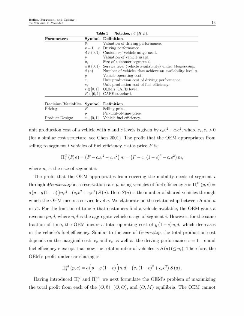
Table 1 Notation, i∈ {H,L}.Parameters Symbol Definition
θi Valuation of driving performance.v= 1− e Driving performance.d∈ (0,1) Customers’ vehicle usage need.ν Valuation of vehicle usage.ni Size of customer segment i.a∈ (0,1) Service level (vehicle availability) under Membership.S (a) Number of vehicles that achieve an availability level a.g Vehicle operating cost.cv Unit production cost of driving performance.ce Unit production cost of fuel efficiency.r ∈ [0,1] OEM’s CAFE level.R ∈ [0,1] CAFE standard.
Decision Variables Symbol DefinitionPricing: F Selling price.
p Per-unit-of-time price.Product Design: e∈ [0,1] Vehicle fuel efficiency.
unit production cost of a vehicle with v and e levels is given by cvv2 + cee
2, where cv, ce > 0
(for a similar cost structure, see Chen 2001). The profit that the OEM appropriates from
selling to segment i vehicles of fuel efficiency e at a price F is:
ΠOi (F, e) =
(F − cvv2− cee2
)ni =
(F − cv (1− e)2− cee2
)ni,
where ni is the size of segment i.
The profit that the OEM appropriates from covering the mobility needs of segment i
through Membership at a reservation rate p, using vehicles of fuel efficiency e is ΠMi (p, e) =
a(p−g (1− e)
)nid− (cvv
2 + cee2)S (a). Here S(a) is the number of shared vehicles through
which the OEM meets a service level a. We elaborate on the relationship between S and a
in §4. For the fraction of time a that customers find a vehicle available, the OEM gains a
revenue pnid, where nid is the aggregate vehicle usage of segment i. However, for the same
fraction of time, the OEM incurs a total operating cost of g (1− e)nid, which decreases
in the vehicle’s fuel efficiency. Similar to the case of Ownership, the total production cost
depends on the marginal costs cv and ce as well as the driving performance v = 1− e and
fuel efficiency e except that now the total number of vehicles is S (a) (≤ ni). Therefore, the
OEM’s profit under car sharing is:
ΠMi (p, e) = a
(p− g (1− e)
)nid−
(cv (1− e)2 + cee
2)S (a) .
Having introduced ΠOi and ΠM
i , we next formulate the OEM’s problem of maximizing
the total profit from each of the (O,∅), (O,O), and (O,M) equilibria. The OEM cannot
Bellos, Ferguson, and Toktay:14 To Sell and to Provide?
directly observe the valuations of each customer. Due to this information asymmetry the
OEM maximizes its profit subject to the individual rationality and incentive compatibility
constraints relevant to each equilibrium. The OEM’s optimization problem associated with
each equilibrium entails the calculation of the fuel efficiencies and prices that will induce
customers to (most profitably for the OEM) self-select into that market equilibrium.
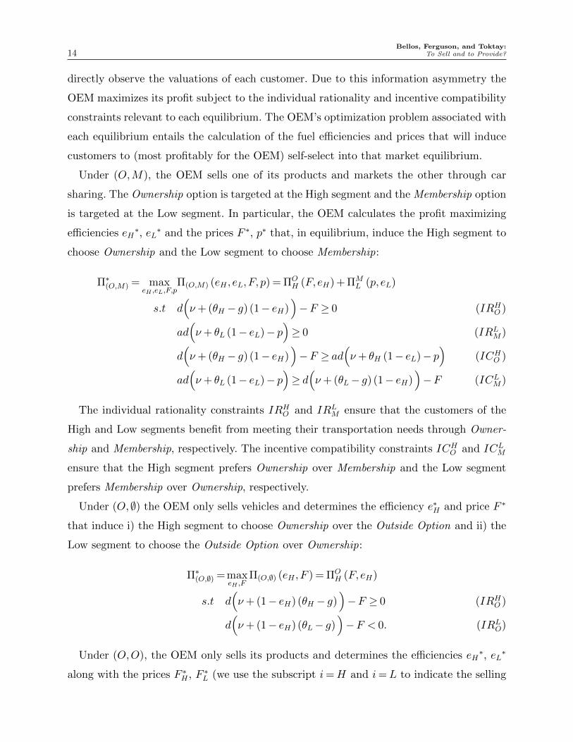
Under (O,M), the OEM sells one of its products and markets the other through car
sharing. The Ownership option is targeted at the High segment and the Membership option
is targeted at the Low segment. In particular, the OEM calculates the profit maximizing
efficiencies eH∗, eL
∗ and the prices F ∗, p∗ that, in equilibrium, induce the High segment to
choose Ownership and the Low segment to choose Membership:
Π∗(O,M) = maxeH ,eL,F,p
Π(O,M) (eH , eL, F, p) = ΠOH (F, eH) + ΠM
L (p, eL)
s.t d(ν+ (θH − g) (1− eH)
)−F ≥ 0 (IRH
O )
ad(ν+ θL (1− eL)− p
)≥ 0 (IRL
M)
d(ν+ (θH − g) (1− eH)
)−F ≥ ad
(ν+ θH (1− eL)− p
)(ICH
O )
ad(ν+ θL (1− eL)− p
)≥ d(ν+ (θL− g) (1− eH)
)−F (ICL
M)
The individual rationality constraints IRHO and IRL
M ensure that the customers of the
High and Low segments benefit from meeting their transportation needs through Owner-
ship and Membership, respectively. The incentive compatibility constraints ICHO and ICL
M
ensure that the High segment prefers Ownership over Membership and the Low segment
prefers Membership over Ownership, respectively.
Under (O,∅) the OEM only sells vehicles and determines the efficiency e∗H and price F ∗
that induce i) the High segment to choose Ownership over the Outside Option and ii) the
Low segment to choose the Outside Option over Ownership:
Π∗(O,∅) = maxeH ,F
Π(O,∅) (eH , F ) = ΠOH (F, eH)
s.t d(ν+ (1− eH) (θH − g)
)−F ≥ 0 (IRH
O )
d(ν+ (1− eH) (θL− g)
)−F < 0. (IRL
O)
Under (O,O), the OEM only sells its products and determines the efficiencies eH∗, eL
∗
along with the prices F ∗H , F ∗L (we use the subscript i=H and i=L to indicate the selling
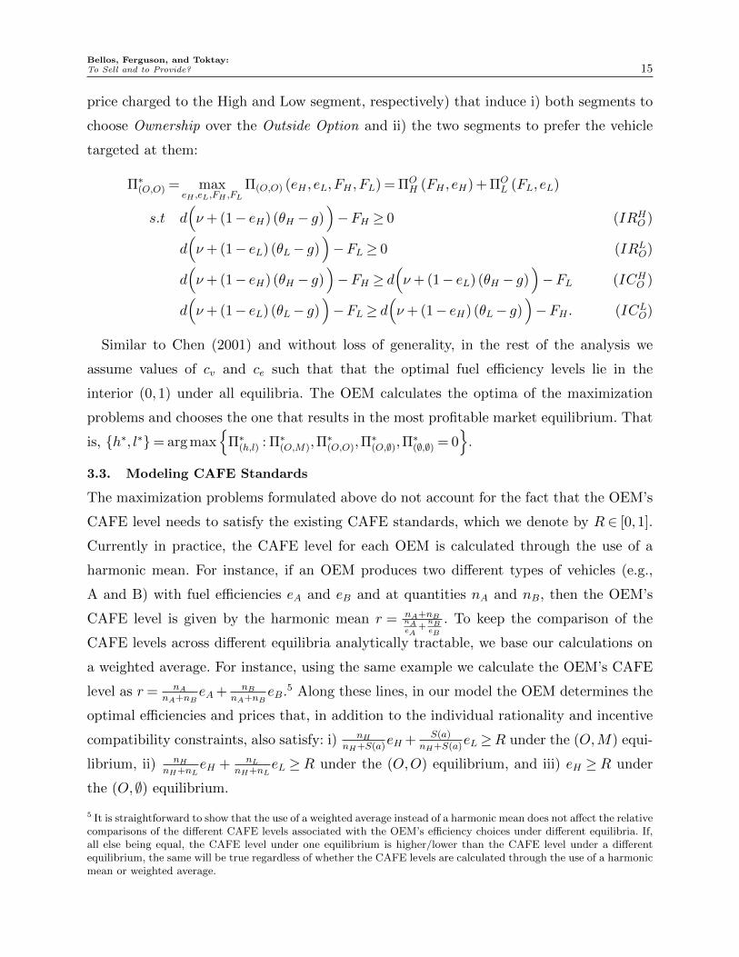
Bellos, Ferguson, and Toktay:To Sell and to Provide? 15
price charged to the High and Low segment, respectively) that induce i) both segments to
choose Ownership over the Outside Option and ii) the two segments to prefer the vehicle
targeted at them:
Π∗(O,O) = maxeH ,eL,FH ,FL
Π(O,O) (eH , eL, FH , FL) = ΠOH (FH , eH) + ΠO
L (FL, eL)
s.t d(ν+ (1− eH) (θH − g)
)−FH ≥ 0 (IRH
O )
d(ν+ (1− eL) (θL− g)
)−FL ≥ 0 (IRL
O)
d(ν+ (1− eH) (θH − g)
)−FH ≥ d
(ν+ (1− eL) (θH − g)
)−FL (ICH
O )
d(ν+ (1− eL) (θL− g)
)−FL ≥ d
(ν+ (1− eH) (θL− g)
)−FH . (ICL
O)
Similar to Chen (2001) and without loss of generality, in the rest of the analysis we
assume values of cv and ce such that that the optimal fuel efficiency levels lie in the
interior (0,1) under all equilibria. The OEM calculates the optima of the maximization
problems and chooses the one that results in the most profitable market equilibrium. That
is, {h∗, l∗}= arg max{
Π∗(h,l) : Π∗(O,M),Π∗(O,O),Π
∗(O,∅),Π
∗(∅,∅) = 0
}.
3.3. Modeling CAFE Standards
The maximization problems formulated above do not account for the fact that the OEM’s
CAFE level needs to satisfy the existing CAFE standards, which we denote by R ∈ [0,1].
Currently in practice, the CAFE level for each OEM is calculated through the use of a
harmonic mean. For instance, if an OEM produces two different types of vehicles (e.g.,
A and B) with fuel efficiencies eA and eB and at quantities nA and nB, then the OEM’s
CAFE level is given by the harmonic mean r = nA+nBnAeA
+nBeB
. To keep the comparison of the
CAFE levels across different equilibria analytically tractable, we base our calculations on
a weighted average. For instance, using the same example we calculate the OEM’s CAFE
level as r= nAnA+nB
eA + nBnA+nB
eB.5 Along these lines, in our model the OEM determines the
optimal efficiencies and prices that, in addition to the individual rationality and incentive
compatibility constraints, also satisfy: i) nHnH+S(a)
eH + S(a)nH+S(a)
eL ≥R under the (O,M) equi-
librium, ii) nHnH+nL
eH + nLnH+nL
eL ≥R under the (O,O) equilibrium, and iii) eH ≥R under
the (O,∅) equilibrium.
5 It is straightforward to show that the use of a weighted average instead of a harmonic mean does not affect the relativecomparisons of the different CAFE levels associated with the OEM’s efficiency choices under different equilibria. If,all else being equal, the CAFE level under one equilibrium is higher/lower than the CAFE level under a differentequilibrium, the same will be true regardless of whether the CAFE levels are calculated through the use of a harmonicmean or weighted average.
Bellos, Ferguson, and Toktay:16 To Sell and to Provide?
4. Analysis and Results
In what follows we analyze the OEM’s optimal business model and product line design
strategy. For the model of car sharing we also characterize the OEM’s optimal capacity
decision. Furthermore, we determine the related economic and environmental implica-
tions, and we examine how such implications depend on the characteristics of the market
served by the OEM as well as the enactment of environmental regulation. When comparing
across different equilibria we utilize the notation (h, l) with h∈ {O} and l ∈ {O,M,∅}. For
instance, eH∗ (O,M) denotes the optimal fuel efficiency of the vehicles sold to the High
segment under the (O,M) equilibrium. All technical proofs and analytical expressions are
relegated to the Appendix.
4.1. Capacity Decisions: The Pooling Effect
Under Membership, if the size of the fleet is S, then at any instance of time the total
number of vehicles in “circulation” (i.e., vehicles that are either idle or being used by the
customers) is also S. This setting resembles the operation of a closed queueing network
with a total of S jobs. Thus, to determine the fleet size that achieves a given service level
a, we model Membership as a two-node closed queueing network and draw on the fixed
population mean (FPM) approximation developed in Whitt (1984).
Remark 1. The OEM’s fleet size that achieves an availability level a when serving
segment i through car sharing is given by S (a)≈ a1−a + anid.
In the Appendix we provide the technical details regarding the development of the
approximation. The second term anid in S (a) represents the number of vehicles required
to meet a service level a when customers’ requests do not overlap. Specifically, nid is the
aggregate vehicle usage generated by ni customers during the useful life of a vehicle, which
also represents the total service load that each vehicle can accommodate. We normalize
the useful life of a vehicle to one. Under “perfect” pooling (i.e., no overlapping customer
requests) the OEM can guarantee a service level a by providing as little as anid vehicles.
The first term a1−a in S (a) is a “correction” term that adjusts this quantity to account for
the fact that, in practice, customer requests may overlap.
Our formulation is based on the aggregate level of a single market (i.e., single geographic
location), and it does not account for capacity allocation issues (e.g., fleet rebalancing)
across different locations within the same market. Such issues are outside the scope of this
paper. For an excellent treatment of such operational considerations, see He et al. (2015).
In what follows we characterize the OEM’s pricing and product design strategy.
Bellos, Ferguson, and Toktay:To Sell and to Provide? 17
4.2. Product Line Decisions: Optimal Pricing and Fuel Efficiency
The OEM cannot observe the preferences θH and θL of individual customers and for that
reason it chooses the prices and the fuel efficiencies of the vehicles such that customers
self-select to a mobility/product design offering. We continue by characterizing the OEM’s
optimal product design (fuel efficiency) choice under each possible market equilibrium. In
the remainder of the paper we assume that nL >1
(1−d)(1−a)because unless this condition
holds the (O,M) equilibrium is always dominated (we elaborate in the Appendix).
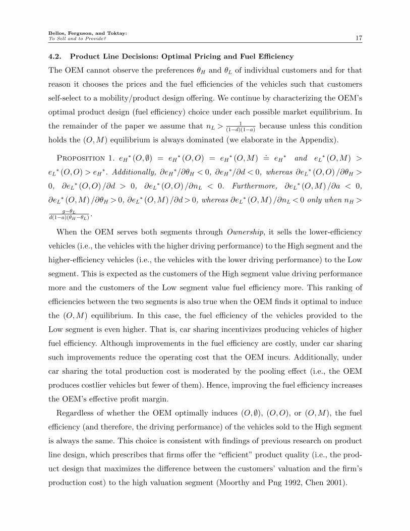
Proposition 1. eH∗ (O,∅) = eH
∗ (O,O) = eH∗ (O,M)
.= eH
∗ and eL∗ (O,M) >
eL∗ (O,O) > eH
∗. Additionally, ∂eH∗/∂θH < 0, ∂eH
∗/∂d < 0, whereas ∂eL∗ (O,O)/∂θH >
0, ∂eL∗ (O,O)/∂d > 0, ∂eL
∗ (O,O)/∂nL < 0. Furthermore, ∂eL∗ (O,M)/∂a < 0,
∂eL∗ (O,M)/∂θH > 0, ∂eL
∗ (O,M)/∂d> 0, whereas ∂eL∗ (O,M)/∂nL < 0 only when nH >
g−θLd(1−a)(θH−θL)
.
When the OEM serves both segments through Ownership, it sells the lower-efficiency
vehicles (i.e., the vehicles with the higher driving performance) to the High segment and the
higher-efficiency vehicles (i.e., the vehicles with the lower driving performance) to the Low
segment. This is expected as the customers of the High segment value driving performance
more and the customers of the Low segment value fuel efficiency more. This ranking of
efficiencies between the two segments is also true when the OEM finds it optimal to induce
the (O,M) equilibrium. In this case, the fuel efficiency of the vehicles provided to the
Low segment is even higher. That is, car sharing incentivizes producing vehicles of higher
fuel efficiency. Although improvements in the fuel efficiency are costly, under car sharing
such improvements reduce the operating cost that the OEM incurs. Additionally, under
car sharing the total production cost is moderated by the pooling effect (i.e., the OEM
produces costlier vehicles but fewer of them). Hence, improving the fuel efficiency increases
the OEM’s effective profit margin.
Regardless of whether the OEM optimally induces (O,∅), (O,O), or (O,M), the fuel
efficiency (and therefore, the driving performance) of the vehicles sold to the High segment
is always the same. This choice is consistent with findings of previous research on product
line design, which prescribes that firms offer the “efficient” product quality (i.e., the prod-
uct design that maximizes the difference between the customers’ valuation and the firm’s
production cost) to the high valuation segment (Moorthy and Png 1992, Chen 2001).
Bellos, Ferguson, and Toktay:18 To Sell and to Provide?
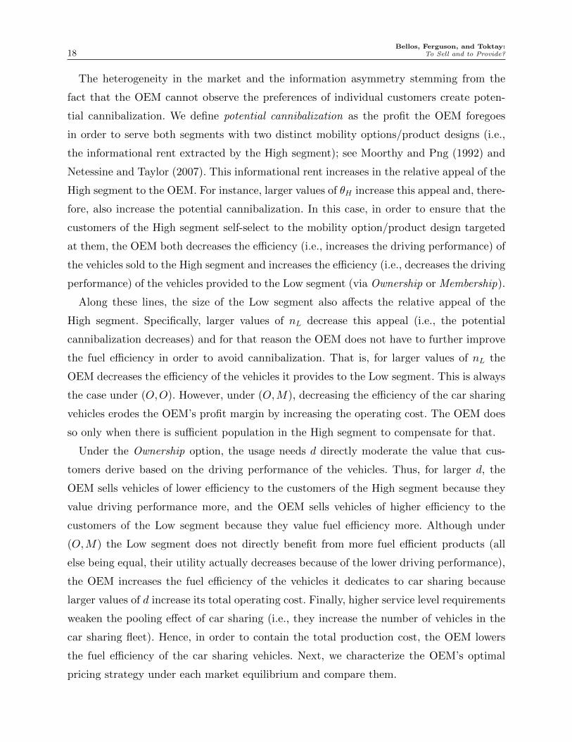
The heterogeneity in the market and the information asymmetry stemming from the
fact that the OEM cannot observe the preferences of individual customers create poten-
tial cannibalization. We define potential cannibalization as the profit the OEM foregoes
in order to serve both segments with two distinct mobility options/product designs (i.e.,
the informational rent extracted by the High segment); see Moorthy and Png (1992) and
Netessine and Taylor (2007). This informational rent increases in the relative appeal of the
High segment to the OEM. For instance, larger values of θH increase this appeal and, there-
fore, also increase the potential cannibalization. In this case, in order to ensure that the
customers of the High segment self-select to the mobility option/product design targeted
at them, the OEM both decreases the efficiency (i.e., increases the driving performance) of
the vehicles sold to the High segment and increases the efficiency (i.e., decreases the driving
performance) of the vehicles provided to the Low segment (via Ownership or Membership).
Along these lines, the size of the Low segment also affects the relative appeal of the
High segment. Specifically, larger values of nL decrease this appeal (i.e., the potential
cannibalization decreases) and for that reason the OEM does not have to further improve
the fuel efficiency in order to avoid cannibalization. That is, for larger values of nL the
OEM decreases the efficiency of the vehicles it provides to the Low segment. This is always
the case under (O,O). However, under (O,M), decreasing the efficiency of the car sharing
vehicles erodes the OEM’s profit margin by increasing the operating cost. The OEM does
so only when there is sufficient population in the High segment to compensate for that.
Under the Ownership option, the usage needs d directly moderate the value that cus-
tomers derive based on the driving performance of the vehicles. Thus, for larger d, the
OEM sells vehicles of lower efficiency to the customers of the High segment because they
value driving performance more, and the OEM sells vehicles of higher efficiency to the
customers of the Low segment because they value fuel efficiency more. Although under
(O,M) the Low segment does not directly benefit from more fuel efficient products (all
else being equal, their utility actually decreases because of the lower driving performance),
the OEM increases the fuel efficiency of the vehicles it dedicates to car sharing because
larger values of d increase its total operating cost. Finally, higher service level requirements
weaken the pooling effect of car sharing (i.e., they increase the number of vehicles in the
car sharing fleet). Hence, in order to contain the total production cost, the OEM lowers
the fuel efficiency of the car sharing vehicles. Next, we characterize the OEM’s optimal
pricing strategy under each market equilibrium and compare them.
Bellos, Ferguson, and Toktay:To Sell and to Provide? 19
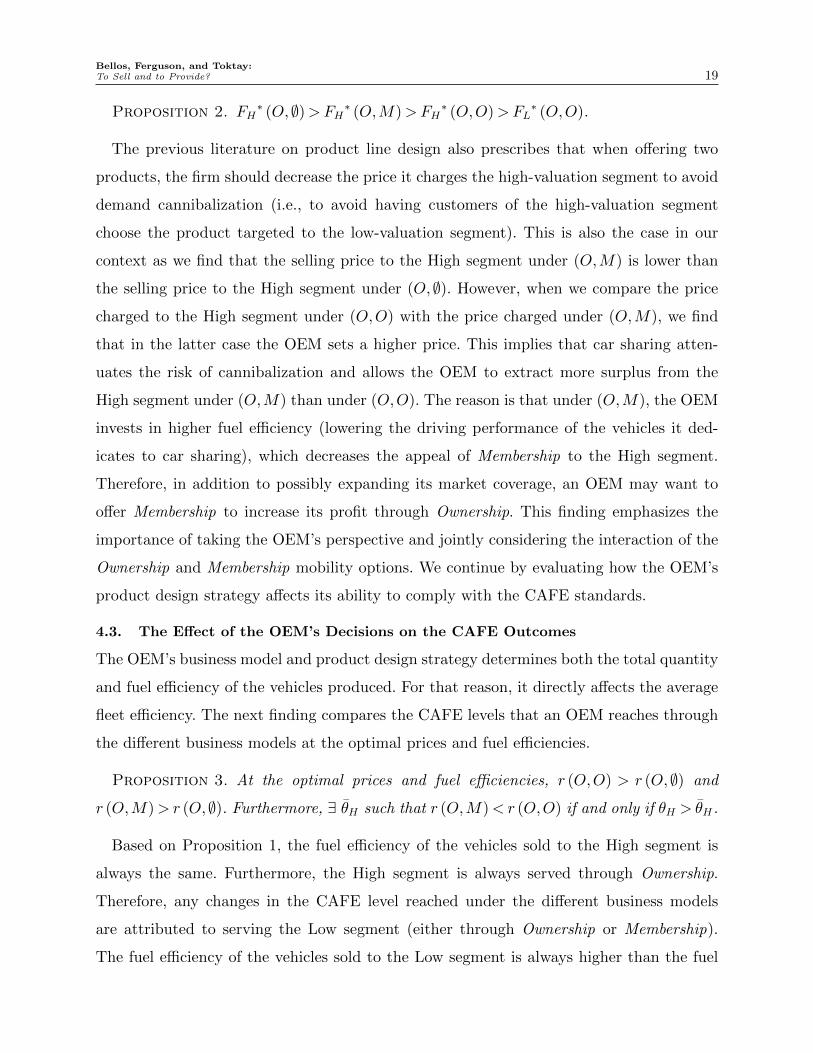
Proposition 2. FH∗ (O,∅)>FH∗ (O,M)>FH
∗ (O,O)>FL∗ (O,O).
The previous literature on product line design also prescribes that when offering two
products, the firm should decrease the price it charges the high-valuation segment to avoid
demand cannibalization (i.e., to avoid having customers of the high-valuation segment
choose the product targeted to the low-valuation segment). This is also the case in our
context as we find that the selling price to the High segment under (O,M) is lower than
the selling price to the High segment under (O,∅). However, when we compare the price
charged to the High segment under (O,O) with the price charged under (O,M), we find
that in the latter case the OEM sets a higher price. This implies that car sharing atten-
uates the risk of cannibalization and allows the OEM to extract more surplus from the
High segment under (O,M) than under (O,O). The reason is that under (O,M), the OEM
invests in higher fuel efficiency (lowering the driving performance of the vehicles it ded-
icates to car sharing), which decreases the appeal of Membership to the High segment.
Therefore, in addition to possibly expanding its market coverage, an OEM may want to
offer Membership to increase its profit through Ownership. This finding emphasizes the
importance of taking the OEM’s perspective and jointly considering the interaction of the
Ownership and Membership mobility options. We continue by evaluating how the OEM’s
product design strategy affects its ability to comply with the CAFE standards.
4.3. The Effect of the OEM’s Decisions on the CAFE Outcomes
The OEM’s business model and product design strategy determines both the total quantity
and fuel efficiency of the vehicles produced. For that reason, it directly affects the average
fleet efficiency. The next finding compares the CAFE levels that an OEM reaches through
the different business models at the optimal prices and fuel efficiencies.
Proposition 3. At the optimal prices and fuel efficiencies, r (O,O) > r (O,∅) and
r (O,M)> r (O,∅). Furthermore, ∃ θH such that r (O,M)< r (O,O) if and only if θH > θH .
Based on Proposition 1, the fuel efficiency of the vehicles sold to the High segment is
always the same. Furthermore, the High segment is always served through Ownership.
Therefore, any changes in the CAFE level reached under the different business models
are attributed to serving the Low segment (either through Ownership or Membership).
The fuel efficiency of the vehicles sold to the Low segment is always higher than the fuel
Bellos, Ferguson, and Toktay:20 To Sell and to Provide?
efficiency of the vehicles sold to the High segment (see Proposition 1) and for that reason,
the OEM always reaches higher CAFE level under (O,O) than under (O,∅).
Proposition 1 also states that the fuel efficiency of the vehicles dedicated to the Low
segment through car sharing under (O,M) is higher than the fuel efficiency of the vehi-
cles sold to the Low segment under (O,O). Proposition 3 reveals that for larger values of
θH , this higher fuel efficiency does not also translate to higher CAFE levels. OEMs serv-
ing customers with higher θH face higher potential cannibalization, which they avoid by
decreasing the fuel efficiency of the vehicles sold to the High segment and by increasing
the fuel efficiency of the vehicles provided (through Ownership or Membership) to the Low
segment. In this manner, the mobility option targeted at the Low segment is less appealing
to the customers of the High segment. Under (O,O), the decrease in the efficiency of the
vehicles sold to the High segment is offset by the increase in the efficiency of the vehicles
sold to the Low segment. However, this is not the case under (O,M). The reason is that
the pooling effect of car sharing (i.e., the fact that the OEM serves the Low segment with
fewer vehicles under (O,M) than under (O,O)) lessens the contribution of these more
fuel-efficient vehicles to the fleet average. In what follows we identify the conditions under
which the OEM introduces each business model.
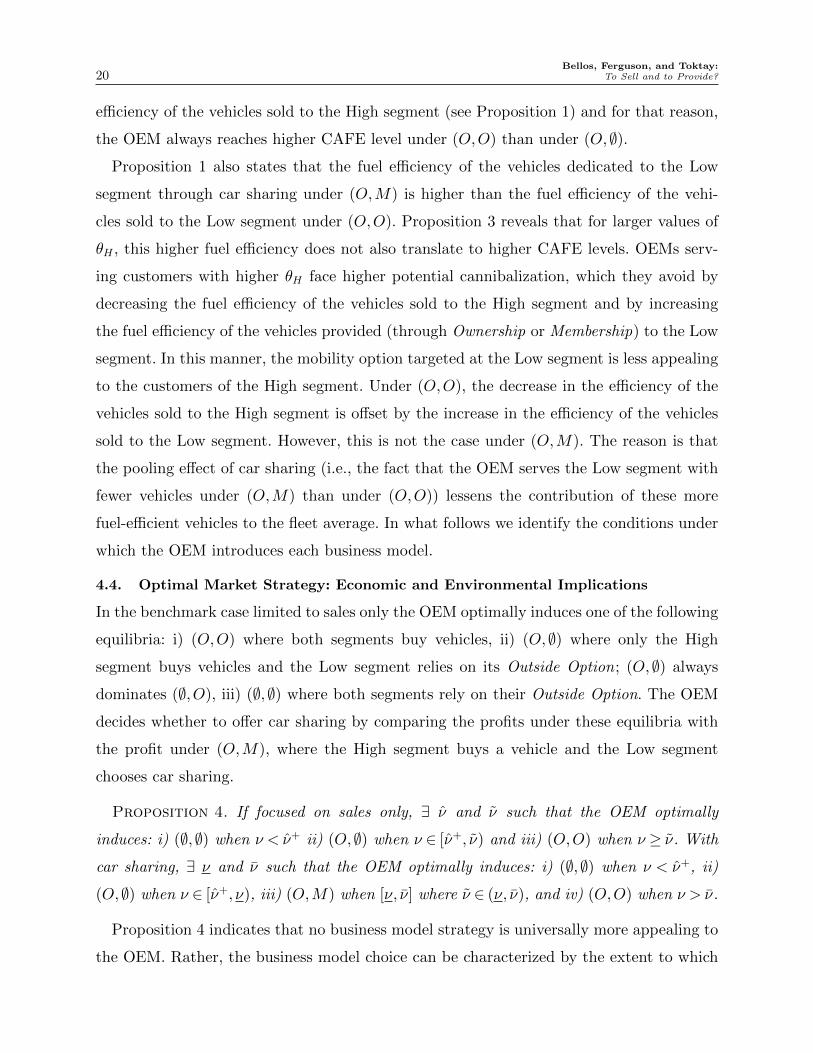
4.4. Optimal Market Strategy: Economic and Environmental Implications
In the benchmark case limited to sales only the OEM optimally induces one of the following
equilibria: i) (O,O) where both segments buy vehicles, ii) (O,∅) where only the High
segment buys vehicles and the Low segment relies on its Outside Option; (O,∅) always
dominates (∅,O), iii) (∅,∅) where both segments rely on their Outside Option. The OEM
decides whether to offer car sharing by comparing the profits under these equilibria with
the profit under (O,M), where the High segment buys a vehicle and the Low segment
chooses car sharing.
Proposition 4. If focused on sales only, ∃ ν and ν such that the OEM optimally
induces: i) (∅,∅) when ν < ν+ ii) (O,∅) when ν ∈ [ν+, ν) and iii) (O,O) when ν ≥ ν. With
car sharing, ∃ ν and ν such that the OEM optimally induces: i) (∅,∅) when ν < ν+, ii)
(O,∅) when ν ∈ [ν+, ν), iii) (O,M) when [ν, ν] where ν ∈ (ν, ν), and iv) (O,O) when ν > ν.
Proposition 4 indicates that no business model strategy is universally more appealing to
the OEM. Rather, the business model choice can be characterized by the extent to which

Bellos, Ferguson, and Toktay:To Sell and to Provide? 21
the customers of each market value vehicle use (see Figure 1). Specifically, in markets with
high valuation of vehicle use, the OEM prefers to sell to both segments: Higher valuation
of use implies that customers derive higher utility from satisfying their mobility needs
per se, as opposed to deriving utility from enjoying the vehicle’s driving performance.
This makes the effect of product differentiation less important and, effectively diminishes
the implications of possible cannibalization, which then allows the OEM to increase its
customer base by selling to both segments. This is not the case for markets with low
valuation of vehicle use: Here, smaller values of ν limit the consumer surplus that the OEM
can extract. Furthermore, in order to appeal to the customers of the Low segment, the
OEM must make costly efficiency improvements. In response, the OEM targets only the
High segment. Figure 1 shows how the OEM’s optimal business model choice changes as
a function of the customers’ valuation of vehicle use.
Figure 1 Market equilibria.
Business model including
car sharing Valuation of use: ν
(O,Ø) (O,O)(O,M)
Business model focused only on selling vehicles Valuation of use: ν
(O,Ø) (O,O)(Ø,Ø)
(Ø,Ø)
:
:ν
Specifically, in Figure 1 we see that car sharing is not necessarily associated with low
valuations of vehicle use, as might be expected due to the fact that customers are not
guaranteed to always find a car available. On the contrary, car sharing can be the optimal
choice in a medium-valuation market. On the one hand, (O,M) may replace (O,∅) when
the valuations of vehicle usage are relatively small but not small enough to deter the OEM
from pursuing additional volume. On the other hand, (O,M) may replace (O,O) when
valuations are relatively large but not large enough to weaken the potential cannibalization.
We now assess the environmental implications of introducing Membership. To this end,
we calculate the environmental impact generated during the production phase, which
depends on the total number of vehicles produced, and during the use phase, which depends
on the aggregate vehicle usage and the fuel efficiency of the vehicles used. In particu-
lar, we define the total environmental impact as E = ζp(Total Production Quantity) +
Bellos, Ferguson, and Toktay:22 To Sell and to Provide?
ζu(e)(Aggregate Usage), where ζp is the unit environmental impact due to production and
ζu(e) is the unit environmental impact (decreasing in the fuel efficiency e) due to use.
Corollary 1. If ν ∈ [ν, ν], introducing car sharing increases the OEM’s profitability
but also its total environmental impact. If ν ∈ (ν, ν], car sharing is a win-win strategy as it
increases the OEM’s profitability and decreases its environmental impact, but it decreases
the OEM’s CAFE level when θH > θH . If the OEM’s CAFE level is calculated based on
the number of customers served (and not on the total number of vehicles produced), then
it always improves under car sharing.
In markets where customers’ valuation of use is such that (O,M) replaces (O,∅) (see
Figure 1), the environmental impact increases due to the market expansion effect (i.e.,
because the Low segment becomes active through Membership). The pooling effect and the
fact that the OEM further improves the efficiency of the vehicles dedicated to Membership
can partially mitigate this increase in the environmental impact, but the net effect is always
environmentally negative. On the other hand, if customers’ valuation of driving is such
that (O,M) replaces (O,O), then the environmental impact always decreases due to both
the pooling effect (i.e., the number of vehicles required to serve the Low segment decreases)
and the fact that the usage needs of the Low segment are satisfied only a fraction of the
time, a (i.e., the aggregate usage of the Low segment decreases). The higher efficiency of
the vehicles dedicated to Membership also contributes to the decrease in the environmental
impact. Therefore, when ν ∈ (ν, ν], introducing Membership is a win-win strategy.
Despite the fact that moving from (O,O) to (O,M) is always environmentally benefi-
cial, higher-end OEMs may realize a decrease in their CAFE levels. This misalignment
is attributed to the way that the CAFE level is calculated, which is based on the total
number of products sold as opposed to the total number of customers served. In other
words, the pooling effect of Membership may actually hinder the OEM’s ability to meet
the enacted standards. In practice, OEMs are penalized based on the extent to which they
do not meet the CAFE standards. Therefore, there may be cases where the transition to
a more sustainable business model such as car sharing may be discouraged due to the
environmental regulation and, specifically, the way that the CAFE level is calculated. This
finding suggests that for each shared car, incentive multipliers should be granted similar
to those currently proposed for advanced technology vehicles (e.g., starting in 2017 each
electric vehicle will count as two vehicles; see U.S. EPA 2012).
Bellos, Ferguson, and Toktay:To Sell and to Provide? 23
We continue by analyzing how the OEM’s strategy (and the economic and environmental
implications of such a strategy) depends on the characteristics of the market served by
the OEM. We have considered the market to be heterogeneous with respect to how much
customers value driving performance. The ranking of the average driving performance
of different OEMs provided by ICCT (2015) indicates that in practice different OEMs
target different market segments. For instance, BMW’s average engine power is larger than
Volkwagen’s, which is larger than Ford’s. Hence, in what follows we refer to the OEMs
who, all else being equal, serve customers with higher values of θH as “higher-end” OEMs.
In our model we have considered the market to be homogeneous with respect to how
much customers value vehicle use ν. However, markets with different locations or demo-
graphics may be characterized by different ν values. Therefore, if for certain OEMs, a
strategy is optimal under a wider range of ν values, then these OEMs benefit more from
such a strategy as they can implement it in more markets. Along these lines, the next
proposition summarizes the OEM’s optimal equilibrium choice with respect to θH .
Proposition 5. ∂ν/∂θH > 0 and ∂ (ν− ν)/∂θH > 0.
The first part of Proposition 5 implies that, if focused only on sales, higher-end OEMs
prefer to serve only the High segment in more markets than lower-end OEMs. That is,
higher-end OEMs benefit more from “excluding” the Low segment and focusing only on
the High segment. This is consistent with findings in the previous literature (Moorthy and
Png 1992, Netessine and Taylor 2007), and is attributed to the fact that a higher valuation
θH increases the potential cannibalization. In such cases, to sell to both segments, the OEM
has to significantly decrease the price it charges the High segment, and for that reason it
induces (O,∅) instead.
The issue of cannibalization is also responsible for the fact that higher-end OEMs offer
car sharing in more markets than lower-end OEMs. This implies that car sharing bene-
fits higher-end OEMs more than lower-end OEMs. In particular, Membership allows for
a better “separation” of the two customer segments and helps minimize the potential
cannibalization. This is due to the cost savings of the pooling effect, which enables the
OEM to choose higher-efficiency vehicles (i.e., vehicles with lower driving performance).
By providing these higher-efficiency vehicles to the Low segment, the OEM discourages the
High segment from relinquishing Ownership for Membership. When switching from (O,∅)
Bellos, Ferguson, and Toktay:24 To Sell and to Provide?
to (O,M), the increase in profitability is attributed to the market expansion effect (i.e.,
the OEM benefits from expanding to the Low segment), and when switching from (O,O),
the increase in profitability is attributed to the pooling effect (i.e., the needs of the Low
segment are met through fewer vehicles) and the higher price charged to the High segment
(see Proposition 1). Our findings in Proposition 5 may help explain why higher-end OEMs
like BMW and Daimler have been particularly active in introducing car sharing programs.
4.5. The Effect of CAFE Regulation on the OEM’s Strategy
To better understand the implications of the CAFE standards, we investigate the optimal
pricing and business model strategy when the OEM is constrained by the enacted regulation
(i.e., when the OEM does not meet the standards at its unconstrained optimal decisions).
Proposition 6. When the CAFE standard is binding at optimality, ∂FH∗ (O,∅)/∂R<
0, ∂FH∗ (O,O)/∂R > 0, and ∂FL
∗ (O,O)/∂R > 0. Furthermore, ∂p∗/∂R < 0 whereas
∂FH∗ (O,M)/∂R< 0 if and only if a< θH−g
g−θL.
Regardless of the market equilibrium, stricter regulation forces the OEM to increase the
fuel efficiency of its vehicles beyond the most profitable levels. It may first appear that
such an increase affects the higher-end OEMs more since it comes at the expense of driving
performance, implying that a decrease in the selling prices may be necessary to maintain
the appeal to the performance-sensitive customers. However, we find that this may not be
always true. Under (O,∅), the OEM indeed lowers the selling price due to the increase in
the fuel efficiency of its vehicles. In contrast, under (O,O), we find that the OEM increases
both the fuel efficiency and the selling prices of its vehicles. In this case, the Low segment
benefits from the higher efficiency, which allows the OEM to charge a higher price and
extract the consumer surplus. Furthermore, although the driving performance of the cars
sold to the High segment is lower under more aggressive CAFE standards, the even higher
fuel efficiency of the vehicles sold to the Low segment makes the customers of the High
segment less willing to switch, allowing the OEM to charge them a higher price.
Under (O,M), the per-unit-of-time price of car sharing decreases. Even though the
customers of the Low segment value fuel efficiency more, under car sharing they do not
derive an immediate additional benefit from using a higher-efficiency vehicle. If anything,
they derive a smaller benefit due to the lower driving performance of the vehicles. Finally, a
higher service level renders car sharing more appealing to customers. For that reason, under
Bellos, Ferguson, and Toktay:To Sell and to Provide? 25
(O,M) and larger values of a, the OEM typically decreases the selling price to discourage
the customers of the High segment from relinquishing Ownership for Membership. Under
more aggressive CAFE standards, however, this appeal is moderated by the higher fuel
efficiency (i.e., lower driving performance) of the vehicles used for car sharing and, thus,
the OEM does not lower its selling price to the High segment.
Proposition 7. If the OEM is focused on sales only and the CAFE standard is binding
at optimality, ∂ν/∂R < 0 for R ∈[r (O,O) , e∗L (O,O)
)and ∂ν/∂R≥ 0 for R≥ e∗L (O,O).
With car sharing, if the CAFE standard is binding at optimality, ∂ (ν− ν)/∂R> 0.
In the case of selling only, the effect of regulation on the optimal business model choice
depends on how aggressive the CAFE standards are. If the standards exceed the CAFE
level that the OEM achieves under (O,O) but are less than the fuel efficiency of the vehicles
sold to the Low segment, then the OEM reacts to stricter standards by replacing (O,∅)
with (O,O). In contrast, if the CAFE standards are even more aggressive and exceed the
efficiency of the vehicles sold to the Low segment, then the OEM reacts by replacing (O,O)
with (O,∅). This happens despite the fact that under (O,O) the OEM increases its selling
prices and sells vehicles of higher driving performance (i.e., lower efficiency) to the High
segment than under (O,∅). The reason is that by selling only to part of the market (i.e.,
only the High segment versus both segments), the OEM limits the increase in the total
production cost due to the higher fuel efficiency. Along similar lines, with car sharing more
aggressive CAFE standards always incentivize the OEM to induce (O,M) in more markets
because the pooling effect attenuates the cost implications of producing higher-efficiency
vehicles. Therefore, including car sharing can be a good strategy to better absorb the cost
implications of abiding by the CAFE standards.
5. Conclusions
This work is motivated by the increasing popularity of car sharing as a viable alternative
to car ownership and the growing involvement of OEMs in the car sharing business. Specif-
ically, in this paper we identify the value that an OEM can derive from introducing car
sharing and characterize the conditions under which this strategy holds the most economic
and environmental potential. We determine the OEM’s optimal choice of business models
and product line by balancing the trade-off between vehicle driving performance and fuel
efficiency. Given the enactment of required CAFE standards and the fact that they are

Bellos, Ferguson, and Toktay:26 To Sell and to Provide?
scheduled to increase steeply in the near future, we also evaluate the effect of regulation on
the OEM’s overall strategy and offer insights with respect to the different types of OEMs
and markets found in practice.
When markets can be categorized based on the valuation customers assign to having
access to a car (which can be a function of other market attributes such as available
parking, public transportation options, etc.), our analysis reveals that OEMs prefer to
introduce car sharing in markets where customers have moderate valuations of vehicle use.
Such a middle ground implies that the OEM should not base its decision to introduce car
sharing in a market entirely on the potential increase in market coverage, as it may actually
benefit from having some existing customers switch from car ownership to car sharing
even if the market is currently fully covered. Furthermore, although car sharing can deter
customers from buying cars, it allows for better price discrimination and enables the OEM
to charge higher prices for the vehicles it sells. Finally, we also find that higher-end OEMs
benefit more from including car sharing in their business models. This is an important
finding as it may help explain why higher-end OEMs such as Daimler and BMW have
been introducing car sharing programs. Our is the first study to characterize the OEM’s
benefits from offering car sharing.
Counter to some recent claims, we find that introducing car sharing does not always
benefit the environment. Even in cases where car sharing is environmentally superior, the
pooling effect of car sharing may actually decrease the OEM’s CAFE level. This find-
ing has clear policy implications as it suggests that OEMs offering car sharing should be
granted incentive multipliers for each shared vehicle they provide. Otherwise, OEMs may
be disincentivized from adopting a car sharing business model despite it being both eco-
nomically and environmentally superior. Finally, car sharing can be a good strategy to
mitigate the loss in profitability resulting from the enactment of more aggressive standards
for an OEM’s CAFE level. This is the first study to identify and characterize the con-
nection between the OEM’s incentive to offer car sharing and the existing environmental
regulation in the automotive industry.
In order to obtain first-order insights, our analysis was conducted in the absence of
competition. Although we expect the presence of competition to further increase the envi-
ronmental impact due to higher market expansion resulting from lower prices, it may also

Bellos, Ferguson, and Toktay:To Sell and to Provide? 27
decrease the OEM’s benefit from offering car sharing. Therefore, future research that incor-
porates competitive pressure from other OEMs or third-party providers may also uncover
valuable insights. Similarly, our analysis was conducted in the absence of channel frictions.
In addition to determining whether to offer car sharing, the OEM may also evaluate differ-
ent supply chain structures. For instance, an OEM may choose to sell vehicles through a
retailer and offer car sharing through a direct channel or sell vehicles and offer car sharing
through the same retailer. This is a promising direction of future research, as also evi-
denced by the fact that in Germany, Ford is currently providing car sharing through its
dealerships (Ford 2015).
Finally, in our customer utility, the vehicle unavailability represented the main form of
customer inconvenience. In practice, customers may experience additional forms of inconve-
nience when meeting their transportation needs through car sharing such as anxiety about
potentially not finding a vehicle available when needed, the need to budget extra commute
time in order to walk to and from the parking lot, feeling pressed to curtail vehicle use
since payment is directly linked to the duration of use, and, the lack of ownership pride.
We expect that, as the model of car sharing matures and car sharing networks continue to
expand in more geographic areas, the importance of some of these factors will diminish over
time. Nevertheless, a more detailed treatment of such inconvenience factors or intangible
benefits such as the satisfaction of adopting green practices presents a promising direction
of future research that can provide additional insights regarding the appeal of car sharing
to customers.
Appendix
In what follows we provide details on the proofs of our results. The analytical expressions
are explicitly given unless they hinder manuscript readability in which case only the short-
hand notation is provided. For instance, instead of providing the complete expression of
the optimal profit under the (O,M) equilibrium we use Π∗(O,M) to denote it. The complete
forms are available from the authors upon request. When comparing across different equi-
libria we utilize the notation (h, l) with h∈ {O} and l ∈ {O,M,∅}. For instance, eH∗ (O,M)
denotes the optimal fuel efficiency of the vehicles sold to the High segment under the
(O,M) equilibrium.
Proof of Remark 1. Assume that each customer requests a vehicle according to a Poisson
process with rate λ′ and that the mean duration of each vehicle use is τ . Set λ′τ.= d,
Bellos, Ferguson, and Toktay:28 To Sell and to Provide?
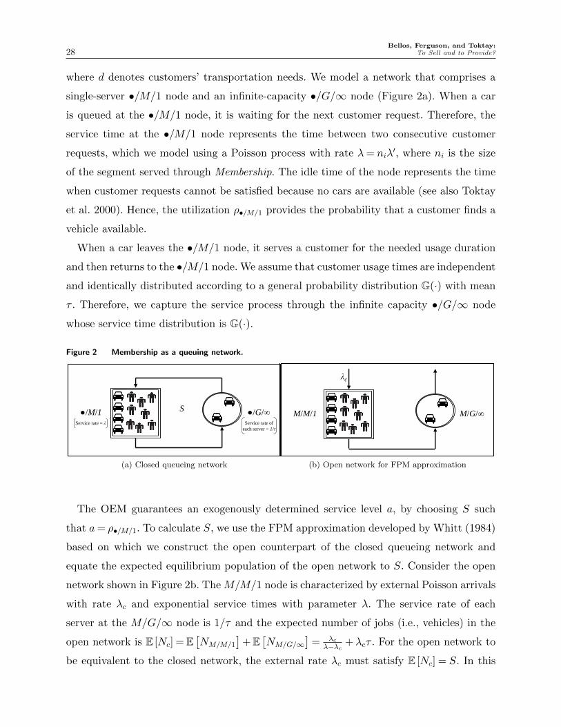
where d denotes customers’ transportation needs. We model a network that comprises a
single-server •/M/1 node and an infinite-capacity •/G/∞ node (Figure 2a). When a car
is queued at the •/M/1 node, it is waiting for the next customer request. Therefore, the
service time at the •/M/1 node represents the time between two consecutive customer
requests, which we model using a Poisson process with rate λ= niλ′, where ni is the size
of the segment served through Membership. The idle time of the node represents the time
when customer requests cannot be satisfied because no cars are available (see also Toktay
et al. 2000). Hence, the utilization ρ•/M/1 provides the probability that a customer finds a
vehicle available.
When a car leaves the •/M/1 node, it serves a customer for the needed usage duration
and then returns to the •/M/1 node. We assume that customer usage times are independent
and identically distributed according to a general probability distribution G(·) with mean
τ . Therefore, we capture the service process through the infinite capacity •/G/∞ node
whose service time distribution is G(·).
Figure 2 Membership as a queuing network.
●/M/1 ●/G/∞ M/M/1 M/G/∞S
λc
Service rate of
each server = 1/τ
Service rate = λ
(a) Closed queueing network
●/M/1 ●/G/∞ M/M/1 M/G/∞S
λc
Service rate of
each server = 1/τ
Service rate = λ
(b) Open network for FPM approximation
The OEM guarantees an exogenously determined service level a, by choosing S such
that a= ρ•/M/1. To calculate S, we use the FPM approximation developed by Whitt (1984)
based on which we construct the open counterpart of the closed queueing network and
equate the expected equilibrium population of the open network to S. Consider the open
network shown in Figure 2b. The M/M/1 node is characterized by external Poisson arrivals
with rate λc and exponential service times with parameter λ. The service rate of each
server at the M/G/∞ node is 1/τ and the expected number of jobs (i.e., vehicles) in the
open network is E [Nc] = E[NM/M/1
]+E
[NM/G/∞
]= λc
λ−λc +λcτ . For the open network to
be equivalent to the closed network, the external rate λc must satisfy E [Nc] = S. In this

Bellos, Ferguson, and Toktay:To Sell and to Provide? 29
case, ρM/M/1 = λcλ
determines the service level, which must equal a. Substituting λc = aλ
in E [Nc] = S results in S (a)≈ a1−a + aλτ . Given that λ
.= niλ
′ and d.= λ′τ , the fleet size
that achieves an availability level a is S (a)≈ a1−a + anid.�
Proof of Propositions 1 and 2. For each possible equilibrium we first determine the
optimal prices and then the optimal fuel efficiencies.
Under (O,∅) and for given efficiencies, the OEM determines the selling price F based
on maxF Π(O,∅) =(F − cv (1− eH)2− ceeH2
)nH subject to the individual rationality con-
straints d(ν + (1− eH) (θH − g)
)−F ≥ 0, and d
(ν − (1− eH) (g− θL)
)−F ≤ 0 which can
be rewritten as d(ν − (1− eH) (g− θL)
)≤ F ≤ d
(ν + (1− eH) (θH − g)
). The profit Π(O,∅)
is linear increasing in F . Therefore, for a given fuel efficiency the optimal selling price
is F = d(ν + (1− eH) (θH − g)
). Define Π(O,∅)
.= Π(O,∅)
(F = F
). Then, the OEM deter-
mines the optimal fuel efficiency based on maxeH Π(O,∅) such that 0 ≤ eH ≤ 1. Π(O,∅) is
concave in the fuel efficiency because ∂2Π(O,∅)/∂2eH =−2 (cv + ce)nH < 0, therefore, after
solving ∂Π(O,∅)/∂eH = 0 we obtain eH∗ = 2cv−d(θH−g)
2(cv+ce). It is straightforward to show that
eH∗ ≥ 0 iff cv ≥ cv
.= d(θH−g)
2> 0 and eH
∗ ≤ 1 iff ce ≥ ce.= −d(θH−g)
2, which is always true
as ce < 0. Following Chen (2001) we focus on interior values of eH∗ ∈ (0,1). Hence, we
assume that cv > cv. Based on eH∗ we also calculate F ∗ = dν +
d(θH−g)(
2ce+d(θH−g))
2(cv+ce)and
Π∗(O,∅) = nH
(dν+
d(θH−g)(
4ce+d(θH−g))−4cvce
4(cv+ce)
).
Under (O,O) and for given efficiencies, the OEM determines the selling prices FH ,
and FL (we use the subscript i = H and i = L to indicate the selling price charged to
the High and Low segment, respectively) based on maxFH ,FL Π(O,O) =(FH − cv (1− eH)2−
ceeH2)nH +
(FL − cv (1− eL)2 − ceeL2
)nL subject to the individual rationality constraints
d(ν + (1− eH) (θH − g)
)− FH ≥ 0 and d
(ν + (1− eL) (θL− g)
)− FL ≥ 0, and the incen-
tive compatibility constraints d(ν+(1− eH) (θH − g)
)−FH ≥ d
(ν+(1− eL) (θH − g)
)−FL
and d(ν + (1− eL) (θL− g)
)− FL ≥ d
(ν + (1− eH) (θL− g)
)− FH . The individual ratio-
nality constraints can be rewritten as FH ≤ d(ν + (1− eH) (θH − g)
)and FL ≤ d
(ν +
(1− eL) (θL− g)). Similarly, the incentive compatibility constraints are rewritten as FL +
d (eH − eL) (g− θL)≤ FH ≤ FL−d (eH − eL) (θH − g), which hold iff eL ≥ eH (we show below
that at optimality eL > eH holds). The profit Π(O,O) is linear increasing in both FH and
FL. Therefore, for given vehicle efficiencies, the optimal selling prices are FL = d(ν +
(1− eL) (θL− g))
and FH = min{FL + d (eL− eH) (θH − g) , d
(ν+ (1− eH) (θH − g)
)},
from which is simple to show that FH = d (v+ (1− eL)θL + (eL− eH)θH − (1− eH)g).
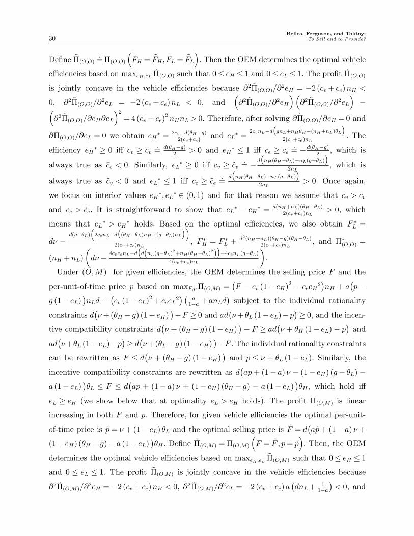
Bellos, Ferguson, and Toktay:30 To Sell and to Provide?
Define Π(O,O).= Π(O,O)
(FH = FH , FL = FL
). Then the OEM determines the optimal vehicle
efficiencies based on maxeH ,eL Π(O,O) such that 0≤ eH ≤ 1 and 0≤ eL ≤ 1. The profit Π(O,O)
is jointly concave in the vehicle efficiencies because ∂2Π(O,O)/∂2eH = −2 (cv + ce)nH <
0, ∂2Π(O,O)/∂2eL = −2 (cv + ce)nL < 0, and
(∂2Π(O,O)/∂
2eH
)(∂2Π(O,O)/∂
2eL
)−(
∂2Π(O,O)/∂eH∂eL
)2
= 4 (cv + ce)2 nHnL > 0. Therefore, after solving ∂Π(O,O)/∂eH = 0 and
∂Π(O,O)/∂eL = 0 we obtain eH∗ = 2cv−d(θH−g)
2(cv+ce)and eL
∗ =2cvnL−d
(gnL+nHθH−(nH+nL)θL
)2(cv+ce)nL
. The
efficiency eH∗ ≥ 0 iff cv ≥ cv
.= d(θH−g)
2> 0 and eH
∗ ≤ 1 iff ce ≥ ce.= −d(θH−g)
2, which is
always true as ce < 0. Similarly, eL∗ ≥ 0 iff cv ≥ cv
.= −d
(nH(θH−θL)+nL(g−θL)
)2nL
, which is
always true as cv < 0 and eL∗ ≤ 1 iff ce ≥ ce
.=
d(nH(θH−θL)+nL(g−θL)
)2nL
> 0. Once again,
we focus on interior values eH∗, eL
∗ ∈ (0,1) and for that reason we assume that cv > cv
and ce > ce. It is straightforward to show that eL∗ − eH∗ = d(nH+nL)(θH−θL)
2(cv+ce)nL> 0, which
means that eL∗ > eH
∗ holds. Based on the optimal efficiencies, we also obtain F ∗L =
dν −d(g−θL)
(2cenL−d
((θH−θL)nH+(g−θL)nL
))2(cv+ce)nL
, F ∗H = F ∗L + d2(nH+nL)(θH−g)(θH−θL)2(cv+ce)nL
, and Π∗(O,O) =
(nH +nL)
(dν− 4cvcenL−d
(d(nL(g−θL)2+nH(θH−θL)2)
)+4cenL(g−θL)
4(cv+ce)nL
).
Under (O,M) for given efficiencies, the OEM determines the selling price F and the
per-unit-of-time price p based on maxF,pΠ(O,M) =(F − cv (1− eH)2 − ceeH2
)nH + a
(p −
g (1− eL))nLd −
(cv (1− eL)2 + ceeL
2) (
a1−a + anLd
)subject to the individual rationality
constraints d(ν+(θH − g) (1− eH)
)−F ≥ 0 and ad
(ν+θL (1− eL)−p
)≥ 0, and the incen-
tive compatibility constraints d(ν + (θH − g) (1− eH)
)− F ≥ ad
(ν + θH (1− eL)− p
)and
ad(ν+θL (1− eL)−p
)≥ d(ν+(θL− g) (1− eH)
)−F . The individual rationality constraints
can be rewritten as F ≤ d(ν + (θH − g) (1− eH)
)and p ≤ ν + θL (1− eL). Similarly, the
incentive compatibility constraints are rewritten as d(ap+ (1− a)ν − (1− eH) (g− θL)−
a (1− eL))θL ≤ F ≤ d
(ap + (1− a)ν + (1− eH) (θH − g) − a (1− eL)
)θH , which hold iff
eL ≥ eH (we show below that at optimality eL > eH holds). The profit Π(O,M) is linear
increasing in both F and p. Therefore, for given vehicle efficiencies the optimal per-unit-
of-time price is p= ν + (1− eL)θL and the optimal selling price is F = d(ap+ (1− a)ν +
(1− eH) (θH − g)− a (1− eL))θH . Define Π(O,M)
.= Π(O,M)
(F = F , p= p
). Then, the OEM
determines the optimal vehicle efficiencies based on maxeH ,eL Π(O,M) such that 0≤ eH ≤ 1
and 0 ≤ eL ≤ 1. The profit Π(O,M) is jointly concave in the vehicle efficiencies because
∂2Π(O,M)/∂2eH = −2 (cv + ce)nH < 0, ∂2Π(O,M)/∂
2eL = −2 (cv + ce)a(dnL + 1
1−a
)< 0, and

Bellos, Ferguson, and Toktay:To Sell and to Provide? 31
(∂2Π(O,M)/∂
2eH
)(∂2Π(O,M)/∂
2eL
)−(∂2Π(O,M)/∂eH∂eL
)2
=4(cv+ce)
2nHa(
1+(1−a)dnL
)1−a > 0.
Therefore, after solving ∂Π(O,M)/∂eH = 0 and ∂Π(O,M)/∂eL = 0 we obtain eH∗ = 2cv−d(θH−g)
2(cv+ce)
and eL∗ =
2cv
(1+(1−a)dnL
)−d(1−a)
((g−θL)nL+(θH−θL)nH
)2(cv+ce)(1+(1−a)dnL)
. The efficiency eH∗ ≥ 0 iff cv ≥ cv
.=
d(θH−g)2
> 0 and eH∗ ≤ 1 iff ce ≥ ce
.=−d(θH−g)
2, which is always true as ce < 0. With respect
to eL∗, in this case we have that eL
∗ ≥ 0 iff cv ≥ cv.=− (1−a)d
((g−θL)nL+(θH−θL)nH
)2(1+(1−a)dnL)
, which is
always true as cv < 0. In addition, eL∗ ≥ 1 iff ce ≥ ce
.=
(1−a)d(
(g−θL)nL+(θH−θL)nH
)2(1+(1−a)dnL)
> 0. As
before, our focus is on interior values eH∗, eL
∗ ∈ (0,1) and for that reason we assume that
cv > cv and ce > ce. Based on the optimal efficiencies we also obtain the optimal prices F ∗
and p∗ along with the optimal profit Π∗(O,M) (analytical expressions available upon request).
Note that the difference ce− ce =d(−1+(1−a)nL(1−d)
)((g−θL)nL+(θH−θL)nH
)2nL(1+(1−a)dnL)
> 0 due to nL >
nL.= 1
(1−d)(1−a)> 0.6 This implies that e∗i (h, l) ∈ (0,1) for all i ∈ {H,L}, h ∈ {O}, and
l ∈ {O,M} when cv > cv and ce >max{ce, ce}= ce.
By comparing the fuel efficiencies under the different market equilibria we find
that eH∗ (O,∅) = eH
∗ (O,O) = eH∗ (O,M) = 2cv−d(θH−g)
2(cv+ce)and eL
∗ (O,O) − eH∗ (O,O) =
d(nH+nL)(θH−θL)2(cv+ce)nL
> 0, therefore, eL∗ (O,O) > eH
∗ (O,O). Similarly, given that nL >
nL, eL∗ (O,M)− eH∗ (O,M) =
d
(θH
(1+dnL+nH−a(dnL+nH)
)+g(
(1−a)(1−d)nL−1)−(1−a)θL(nH+nL)
)2(cv+ce)(1+(1−a)dnL)
>
0 and eL∗ (O,M) − eL
∗ (O,O) =d(−1+(1−d)nL(1−a)
)((g−θL)nL+(θH−θL)θH
)2(cv+ce)nL(1+(1−a)dnL)
> 0, hence,
eL∗ (O,M)> eH
∗ (O,M) and eL∗ (O,M)> eL
∗ (O,O).
In terms of comparative statics we obtain: ∂eH∗/∂θH = − d
2(cv+ce)< 0, ∂eH
∗/∂d =
− θH−g2(cv+ce)
< 0, ∂eL∗ (O,O)/∂θH = dnH
2(cv+ce)nL> 0, ∂eL
∗ (O,O)/∂d = (θH−θL)nH+(g−θL)nL2(cv+ce)nL
>
0, ∂eL∗ (O,O)/∂nL = −dnH(θH−θL)
2(cv+ce)n2L< 0, ∂eL
∗ (O,M)/∂a = −d(
(θH−θL)nH+(g−θL)nL
)2(cv+ce)(1+dnL(1−a))2
< 0,
∂eL∗ (O,M)/∂θH = dnH(1−a)
2(cv+ce)(1+dnL(1−a))> 0, ∂eL
∗ (O,M)/∂d=(1−a)
((θH−θL)nH+(g−θL)nL
)2(cv+ce)(1+dnL(1−a))2
> 0,
and ∂eL∗ (O,M)/∂nL =
d(1−a)(g−θL−dnH(1−a)(θH−θL)
)2(cv+ce)(1+dnL(1−a))2
> 0 iff nH <g−θL
d(1−a)(θH−θL).
Using a similar notation to distinguish between the prices under different equi-
libria we have, F ∗H (O,O) − F ∗L (O,O) = d2(nH+nL)(θH−g)(θH−θL)2(cv+ce)nL
> 0, F ∗H (O,M) −
F ∗H (O,O) =d(θH−θL)
(2(1−a)cenL
(1+(1−a)dnL
)+d(
(1−a)nL(a−d)−1)(
(θH−θL)nH+(g−θL)nL
))2nL(cv+ce)((1−a)dnL+1)
>
0 due to ce > ce and nL > nL, and F ∗H (O,∅) − F ∗H (O,M) =
6 As we have already stated in §4.2 of the main paper, throughout the analysis we assume that nL > nL, otherwise(O,M) is always dominated (the derivation of the condition is provided in the proof of Proposition 4).
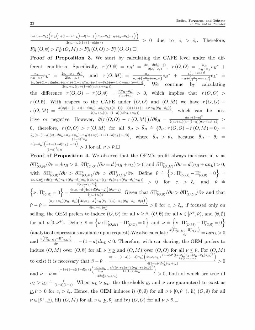
Bellos, Ferguson, and Toktay:32 To Sell and to Provide?
da(θH−θL)
(2ce
(1+(1−a)dnL
)−d(1−a)
((θH−θL)nH+(g−θL)nL
))2(cv+ce)(1+(1−a)dnL)
> 0 due to ce > ce. Therefore,
F ∗H (O,∅)>F ∗H (O,M)>F ∗H (O,O)>F ∗L (O,O).�
Proof of Proposition 3. We start by calculating the CAFE level under the dif-
ferent equilibria. Specifically, r (O,∅) = eH∗ = 2cv−d(θH−g)
2(cv+ce), r (O,O) = nH
nH+nLeH∗ +
nLnH+nL
eL∗ = 2cv−d(g−θL)
2(cv+ce), and r (O,M) = nH
nH+( a1−a+anLd)
eH∗ +
a1−a+anLd
nH+( a1−a+anLd)
eL∗ =
2cv(a+(1−a)(adnL+nH))+(1−a)d(nH(a(θH−θL)+g−θH)+anL(g−θL))2(cv+ce)(a+(1−a)(adnL+nH))
. We continue by calculating
the difference r (O,O) − r (O,∅) = d(θH−θL)2(cv+ce)
> 0, which implies that r (O,O) >
r (O,∅). With respect to the CAFE under (O,O) and (O,M) we have r (O,O) −
r (O,M) =d(ag(1−(1−a)(1−d)nL)−aθL(nL((a−1)(1−d))+1)+(1−a)2nH(θH−θL))
2(cv+ce)(a+(1−a)(adnL+nH)), which can be pos-
itive or negative. However, ∂(r (O,O) − r (O,M)
)/∂θH = dnH(1−a)2
2(cv+ce)(a+(1−a)(nH+adnL))>
0, therefore, r (O,O) > r (O,M) for all θH > θH.= {θH : r (O,O)− r (O,M) = 0} =
θL(a−(1−a)(a(−dnL+nH+nL)−nH))+ag(−1+(1−a)nL(1−d))(1−a)2nH
, where θH > θL because θH − θL =
a(g−θL)(−1+(1−d)nL(1−a)
)(1−a)2nH
> 0 for all ν > ν.�
Proof of Proposition 4. We observe that the OEM’s profit always increases in ν as
∂Π∗(O,∅)/∂ν = dnH > 0, ∂Π∗(O,O)/∂ν = d (nH +nL)> 0 and ∂Π∗(O,M)/∂ν = d (nH + anL)> 0,
with ∂Π∗(O,∅)/∂ν > ∂Π∗(O,M)/∂ν > ∂Π∗(O,O)/∂ν. Define ν.={ν : Π∗(O,O)−Π∗(O,∅) = 0
}=
4cvcen2L+d((g−θL)nL+(θH−θL)nH)(4cenL−((g−θL)nL+(θH−θL)nH))
4(cv+ce)dn2L
> 0 for ce > ce and ν.={
ν : Π∗(O,∅) = 0}
=4cvce−d
(4ce+d(θH−g)
)(θH−g)
4(cv+ce)d. Given that ∂Π∗(O,∅)/∂ν > ∂Π∗(O,O)/∂ν and that
ν − ν =(nH+nL)(θH−θL)
(4cenL+d
(nH(θL−θH)+nL(θH+θL−2g)
))4(cv+ce)n2
L> 0 for ce > ce, if focused only on
selling, the OEM prefers to induce (O,O) for all ν ≥ ν, (O,∅) for all ν ∈ [ν+, ν), and (∅,∅)
for all ν [0, ν+). Define ν.={ν : Π∗(O,M)−Π∗(O,O) = 0
}and ν
.={ν : Π∗(O,M)−Π∗(O,∅) = 0
}(analytical expressions available upon request).We also calculate
d(Π∗(O,M)
−Π∗(O,∅))
dν= adnL > 0
andd(Π∗
(O,M)−Π∗
(O,O))dν
=− (1− a)dnL < 0. Therefore, with car sharing, the OEM prefers to
induce (O,M) over (O,∅) for all ν ≥ ν and (O,M) over (O,O) for all ν ≤ ν. For (O,M)
to exist it is necessary that ν − ν =a(−1+(1−a)(1−d)nL)
(4cvcenL+
(1−a)d2((g−θL)nL+(θH−θL)nH)2
1+(1−a)dnL
)4(1−a)2dn2
L(cv+ce)> 0
and ν − ν =(−1+(1−a)(1−d)nL)
(4cvcenL
1−a +d2((g−θL)nL+(θH−θL)nH)2
1+(1−a)dnL
)4dn2
L(cv+ce)> 0, both of which are true iff
nL > nL.= 1
(1−d)(1−a). When nL > nL, the thresholds ν, and ν are guaranteed to exist as
ν, ν > 0 for ce > ce. Hence, the OEM induces i) (∅,∅) for all ν ∈ [0, ν+), ii) (O,∅) for all
ν ∈ [ν+, ν), iii) (O,M) for all ν ∈ [ν, ν] and iv) (O,O) for all ν > ν.�
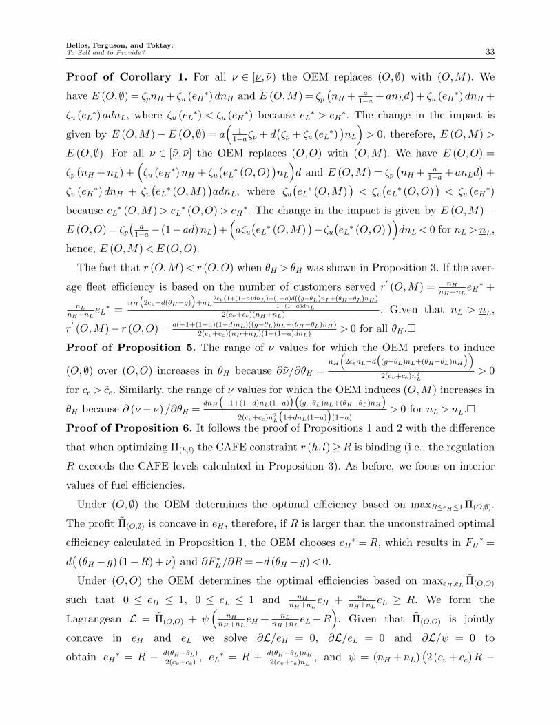
Bellos, Ferguson, and Toktay:To Sell and to Provide? 33
Proof of Corollary 1. For all ν ∈ [ν, ν) the OEM replaces (O,∅) with (O,M). We
have E (O,∅) = ζpnH + ζu (eH∗)dnH and E (O,M) = ζp
(nH + a
1−a + anLd)
+ ζu (eH∗)dnH +
ζu (eL∗)adnL, where ζu (eL
∗) < ζu (eH∗) because eL
∗ > eH∗. The change in the impact is
given by E (O,M)−E (O,∅) = a(
11−aζp + d
(ζp + ζu (eL
∗))nL
)> 0, therefore, E (O,M) >
E (O,∅). For all ν ∈ [ν, ν] the OEM replaces (O,O) with (O,M). We have E (O,O) =
ζp (nH +nL) +(ζu (eH
∗)nH + ζu(eL∗ (O,O)
)nL
)d and E (O,M) = ζp
(nH + a
1−a + anLd)
+
ζu (eH∗)dnH + ζu
(eL∗ (O,M)
)adnL, where ζu
(eL∗ (O,M)
)< ζu
(eL∗ (O,O)
)< ζu (eH
∗)
because eL∗ (O,M)> eL
∗ (O,O)> eH∗. The change in the impact is given by E (O,M)−
E (O,O) = ζp(
a1−a− (1− ad)nL
)+(aζu(eL∗ (O,M)
)−ζu
(eL∗ (O,O)
))dnL < 0 for nL >nL,
hence, E (O,M)<E (O,O).
The fact that r (O,M)< r (O,O) when θH > θH was shown in Proposition 3. If the aver-
age fleet efficiency is based on the number of customers served r′(O,M) = nH
nH+nLeH∗ +
nLnH+nL
eL∗ =
nH
(2cv−d(θH−g)
)+nL
2cv(1+(1−a)dnL)+(1−a)d((g−θL)nL+(θH−θL)nH)1+(1−a)dnL
2(cv+ce)(nH+nL). Given that nL > nL,
r′(O,M)− r (O,O) = d(−1+(1−a)(1−d)nL)((g−θL)nL+(θH−θL)nH)
2(cv+ce)(nH+nL)(1+(1−a)dnL)> 0 for all θH .�
Proof of Proposition 5. The range of ν values for which the OEM prefers to induce
(O,∅) over (O,O) increases in θH because ∂ν/∂θH =nH
(2cenL−d
((g−θL)nL+(θH−θL)nH
))2(cv+ce)n2
L> 0
for ce > ce. Similarly, the range of ν values for which the OEM induces (O,M) increases in
θH because ∂ (ν− ν)/∂θH =dnH
(−1+(1−d)nL(1−a)
)((g−θL)nL+(θH−θL)nH
)2(cv+ce)n2
L
(1+dnL(1−a)
)(1−a)
> 0 for nL >nL.�
Proof of Proposition 6. It follows the proof of Propositions 1 and 2 with the difference
that when optimizing Π(h,l) the CAFE constraint r (h, l)≥R is binding (i.e., the regulation
R exceeds the CAFE levels calculated in Proposition 3). As before, we focus on interior
values of fuel efficiencies.
Under (O,∅) the OEM determines the optimal efficiency based on maxR≤eH≤1 Π(O,∅).
The profit Π(O,∅) is concave in eH , therefore, if R is larger than the unconstrained optimal
efficiency calculated in Proposition 1, the OEM chooses eH∗ =R, which results in FH
∗ =
d(
(θH − g) (1−R) + ν)
and ∂F ∗H/∂R=−d (θH − g)< 0.
Under (O,O) the OEM determines the optimal efficiencies based on maxeH ,eL Π(O,O)
such that 0 ≤ eH ≤ 1, 0 ≤ eL ≤ 1 and nHnH+nL
eH + nLnH+nL
eL ≥ R. We form the
Lagrangean L = Π(O,O) + ψ(
nHnH+nL
eH + nLnH+nL
eL−R)
. Given that Π(O,O) is jointly
concave in eH and eL we solve ∂L/eH = 0, ∂L/eL = 0 and ∂L/ψ = 0 to
obtain eH∗ = R − d(θH−θL)
2(cv+ce), eL
∗ = R + d(θH−θL)nH2(cv+ce)nL
, and ψ = (nH +nL)(2 (cv + ce)R −
Bellos, Ferguson, and Toktay:34 To Sell and to Provide?
2cv − d (g− θL))> 0 for all R > r (O,O). Based on these values we also
obtain FH∗ = d
((g− θL)R+ 2(cv+ce)nL(θL−g+v)+d(θH−θL)((θH−θL)+(θH−g)nL)
2nL(cv+ce)
), FL
∗ = FH∗ −
d2(nH+nL)(θH−g)(θH−θL)2(cv+ce)nL
and ∂F ∗H (O,O)/∂R= ∂F ∗L (O,O)/∂R= d (g− θL)> 0.
Under (O,M) the OEM determines the optimal efficiencies based on maxeH ,eL Π(O,M)
such that 0 ≤ eH ≤ 1, 0 ≤ eL ≤ 1 and nHnH+( a
1−a+anLd)eH +
a1−a+anLd
nH+( a1−a+anLd)
eL ≥ R. The
Lagrangean is given by L = Π(O,M) + ψ
(nH
nH+( a1−a+anLd)
eH +a
1−a+anLd
nH+( a1−a+anLd)
eL−R)
. Once
again, given that Π(O,M) is jointly concave in eH and eL we solve ∂L/eH = 0, ∂L/eL = 0 and
∂L/ψ = 0 to obtain eH∗ = R − ad(θH(−a(dnL+nH)+dnL+nH+1)+g((1−a)(1−d)nL−1)−(1−a)θL(nH+nL))
2(cv+ce)(a+(1−a)(adnL+nH)),
eL∗ = R + (1−a)dnH(θH((1−a)dnL+(1−a)nH+1)−g(nL(a−ad+d−1)+1)−(1−a)θL(nH+nL))
2(cv+ce)((1−a)dnL+1)(a+(1−a)(adnL+nH)), and ψ =
2cv(1−R)((a−1)(adnL+nH)−a)−(1−a)d(anL(−2ceR−θL+g)+nH((a−1)θH−aθL+g))+2ceR((1−a)nH+a)1−a > 0 for all
R> r (O,M). The analytical expressions for FH∗ and p∗ are available upon request. By dif-
ferentiating we obtain ∂p∗/∂R=−θL < 0, and ∂F ∗H (O,M)/∂R= d(g−
(1− a
)θH−aθL
)<
0 iff a< θH−gθH−θL
∈ (0,1).�
Proof of Proposition 7. For brevity define Π∗(O,∅), Π∗(O,O), and Π∗(O,M) to be the uncon-
strained optimal profits we developed in the Proof of Propositions 1 and 2 for the (O,∅),
(O,O), and (O,M) equilibrium, respectively. Using the optimal prices and fuel efficiencies
we calculated in Proposition 6 we obtain the constrained optimal profits Π∗(O,∅) = Π∗(O,∅)−nH
(2cv−2(cv+ce)R−d(θH−g)
)24(cv+ce)
, Π∗(O,O) = Π∗(O,O) −(nH+nL)
(2cv−2(cv+ce)R−d(g−θL)
)24(cv+ce)
, and Π∗(O,M) =
Π∗(O,M)−(
2cv(1−R)((1−a)(adnL+nH)+a)+(1−a)d(anL(−2ceR−θL+g)+nH((a−1)θH−aθL+g))−2ceR((1−a)nH+a))2
4(1−a)(cv+ce)(a+(1−a)(adnL+nH)).
Paralleling Proposition 4, we calculate ν.=
{ν : Π∗(O,O)−Π∗(O,∅) = 0
}, ν
.={
ν : Π∗(O,M)−Π∗(O,∅) = 0}
and ν.={ν : Π∗(O,O)−Π∗(O,M) = 0
}. When selling only r (O,O) >
r (O,∅) (see Proposition 3), hence, the CAFE standard is binding for either equilib-
rium when R ≥ r (O,O). ν is convex in R because ∂2ν/∂R2 = 2(cv+ce)d
> 0. In addition,
∂ν/∂R|R=e∗L(O,O) = 0. Therefore, ∂ν/∂R > 0 for all R ≥ e∗L (O,O) and ∂ν/∂R < 0 for
all R ∈[r (O,O) , e∗L (O,O)
). With car sharing r (O,M) < r (O,O) for θH > θH and
r (O,M) > r (O,O) for θH < θH (see Proposition 3). Hence, for θH > θH the CAFE
standard is binding when R ≥ r (O,O). The range ν − ν is convex in R because ∂2(ν −
ν)/∂2R =
2(cv+ce)(−1+(1−d)nL(1−a)
)dnL(1−a)2
> 0 for nL > nL. Furthermore, ∂(ν − ν
)/∂R|R=r(O,O) =
d(g−θL)(−1+(1−d)nL(1−a)
)2(1−a)2dnL
> 0 for nL > nL. Therefore, ∂(ν − ν
)/∂R > 0 for all R > r (O,O).
Similarly, for θH < θH the CAFE standard is binding when for R ≥ r (O,M). In this
Bellos, Ferguson, and Toktay:To Sell and to Provide? 35
case, ∂(ν − ν
)/∂R|R=r(O,M) =
(−1+(1−a)nL(1−d)
)(nH
(a(θH−θL)−(θH−g)
)+anL(g−θL)
)(1−a)nL
((1−a)(adnL+nH)+a
) > 0 for
nL >nL and θH < θH . Therefore, ∂2(ν− ν
)/∂2R=
2(cv+ce)(−1+(1−d)nL(1−a)
)dnL(1−a)2
> 0 implies that
∂(ν− ν
)/∂R> 0 for all R> r (O,M). Thus, ∂
(ν− ν
)/∂R> 0 for all θH .�
References
Agrawal, V., I. Bellos. 2015. The Potential of Servicizing as a Green Business Model. Forthcoming in
Management Sci.
Agrawal, V., M. Ferguson, B. Toktay, V. Thomas. 2012. Is Leasing Greener Than Selling? Management Sci.
58(3) 523–533.
Ata, B., D. Lee, M. Tongarlak. 2012. Optimizing Organic Waste to Energy Operations. Manufacturing
Service Oper. Management 14(2) 231–244.
Avci, B., K. Girotra, S. Netessine. 2015. Electric Vehicles with a Switching Station: Adoption and Environ-
mental Impact. Management Sci. 61(4) 772–794.
Berry, S., J. Levinsohn, A. Pakes. 1995. Automobile Prices in Market Equilibrium. Econometrica. 841–890.
Biller, S., J. Swann. 2006. Pricing for Environmental Compliance in the Auto Industry. Interfaces 36(2)
118–125.
Boyd, H., R. Mellman. 1980. The Effect of Fuel Economy Standards on The US Automotive Market: An
Hedonic Demand Analysis. Transportation Research Part A: General 14(5) 367–378.
Businessweek. 2013. Steve Case on Avis, Zipcar, and the Sharing Economy. http://www.businessweek.
com/articles/2013-01-02/with-zipcar-avis-backs-steve-cases-sharing-economy.
CAR2GO. 2016. Simply. Always. Everywhere. http://www.car2go.com.
Cervero, R., A. Golub, B. Nee. 2007. City CarShare: Longer-Term Travel Demand and Car Ownership
Impacts. Transp. Res. Record 1992(1) 70–80.
Chan, T., F. DeVericourt, O. Besbes. 2014. Contracting in Medical Equipment Maintenance Services: An
Empirical Investigation. ESMT Working Paper No. 14-05.
Chen, C. 2001. Design for the Environment: A Quality-Based Model for Green Product Development.
Management Sci. 47(2) 250–263.
ConsumerReports. 2015. Owner Satisfaction. http://www.consumerreports.org/cro/
chevrolet-equinox-owner-satisfaction.htm.
Corbett, C., G. DeCroix. 2001. Shared-Savings Contracts for Indirect Materials in Supply Chains: Channel
Profits and Environmental Impacts. Management Sci. 47(7) 881–893.
Corbett, C., G. DeCroix, A. Ha. 2005. Optimal Shared-Savings Contracts in Supply Chains: Linear Contracts
and Double Moral Hazard. Eur. J. Oper. Res. 163(3) 653–667.
Bellos, Ferguson, and Toktay:36 To Sell and to Provide?
Drake, D. 2015. Carbon Tariffs: Effects in Settings with Technology Choice and Foreign Comparative
Advantage. Harvard Business School Technology & Operations Mgt. Unit Working Paper No. 13-021.
DriveNow. 2015. Thank You San Francisco Bay Area. http://www.drive-nowusa.com/.
Edmunds. 2013. FAQ: New Corporate Average Fuel Economy Standards. http://www.edmunds.com/
fuel-economy/faq-new-corporate-average-fuel-economy-standards.html.
Esenduran, Gokce, Eda Kemahlıoglu-Ziya. 2015. A Comparison of Product Take-Back Compliance Schemes.
Production and Oper. Management 24(1) 71–88.
Fishbein, B., L. McGarry, P. Dillon. 2000. Leasing: A Step towards Producer Responsibility. Tech. rep.,
INFORM, Inc.
Ford. 2015. Mobility Experiment: FORD Carsharing, Germany. https://media.ford.com/content/
fordmedia/fna/us/en/news/2015/01/06/mobility-experiment-ford-charsharing-germany.
html.
Fortune. 2015. How Ford’s Chief Became a Tech CEO. http://fortune.com/2015/04/24/
mark-fields-ford-ceo/.
Frei, F.X. 2005. Zipcar: Influencing Customer Behavior. Harvard Business School Case Study 9-605-054,
Harvard University, Cambridge, MA.
Girotra, K., S. Netessine. 2013. OM Forum–Business Model Innovation for Sustainability. Manufacturing
Service Oper. Management 15(4) 537–544.
Guajardo, J., M. Cohen, S. Kim, S. Netessine. 2012. Impact of Performance-based Contracting on Product
Reliability: An Empirical Analysis. Management Sci. 58(5) 961–979.
Guajardo, J., M. Cohen, S. Netessine. 2015. Service Competition and Product Quality in the US Automobile
Industry. Forthcoming in Management Sci.
He, L., H. Mak, Y. Rong, Z. Shen. 2015. Service Region Design for Urban Electric Vehicle Sharing Systems.
Working Paper.
Huang, X., A. Atasu, Toktay B. 2015. Design Implications of Extended Producer Responsibility for Durable
Products. Working Paper.
ICCT. 2015. European Vehicle Market Statistics. http://theicct.org/sites/default/files/
publications/ICCT_EU-pocketbook_2015.pdf.
Jacobsen, M., A. van Benthem. 2015. Vehicle Scrappage and Gasoline Policy. Amer. Econom. Rev. 105(3)
1312–38.
Kabra, A., E. Belavina, K. Girotra. 2015. Bike Share Systems: Accessibility and Availability. Chicago Booth
Research Paper No. 15-04.
Kim, S., M. Cohen, S. Netessine. 2007. Performance Contracting in After-sales Service Supply Chains.
Management Sci. 53(12) 1843–1858.
Bellos, Ferguson, and Toktay:To Sell and to Provide? 37
Kraft, T., F. Erhun, R. Carlson, D. Rafinejad. 2013. Replacement Decisions for Potentially Hazardous
Substances. Production and Oper. Management 22(4) 958–975.
Lifset, R., T. Lindhqvist. 1999. Does Leasing Improve End of Product Life Management? J. Ind. Ecol. 3(4)
10–13.
Lim, M., H. Mak, Y. Rong. 2015. Toward Mass Adoption of Electric Vehicles: Impacts of the Range and
Resale Anxieties. Manufacturing Service Oper. Management 17(1) 101–119.
Michalek, J., P. Papalambros, S. Skerlos. 2004. A Study of Fuel Efficiency and Emission Policy Impact on
Optimal Vehicle Design Decisions. J. Mech. Design 126(6) 1062–1070.
Millard-Ball, A., G. Murray, J. Ter Schure, C. Fox, J. Burkhardt. 2005. TCRP Report 108: Car-Sharing:
Where and How It Succeeds. Transportation Research Board of the National Academies.
Moorthy, K. 1988. Product and Price Competition in a Duopoly. Marketing Sci. 7(2) 141–168.
Moorthy, K., I. Png. 1992. Market Segmentation, Cannibalization, and the Timing of Product Introductions.
Management Sci. 38(3) 345–359.
Mu. 2016. Mu by Peugeot. http://www.mu.peugeot.co.uk/.
Navigant Research. 2013. Carsharing Programs. http://www.navigantresearch.com/wp-content/
uploads/2013/08/CSHP-13-Executive-Summary.pdf.
Netessine, S., T. Taylor. 2007. Product Line Design and Production Technology. Marketing Sci. 26(1)
101–117.
NHTSA. 2014. Summary of Fuel Efficiency Performance. http://www.nhtsa.gov/staticfiles/
rulemaking/pdf/cafe/Performance-summary-report-12152014-v2.pdf.
NHTSA. 2015. CAFE-Fuel Economy. http://www.nhtsa.gov/fuel-economy.
Plambeck, E., Q. Wang. 2009. Effects of E-Waste Regulation on New Product Introduction. Management
Sci. 55(3) 333–347.
Quicar. 2016. Quicar-Share a Volkswagen. https://web.quicar.de/.
Rothenberg, S. 2007. Sustainability Through Servicizing. MIT Sloan Manage. Rev. 48(2) 83–91.
Shaheen, P., A. Cohen. 2015. Innovative Mobility Carsharing Outlook. http://innovativemobility.org/
wp-content/uploads/2015/07/Summer-2015-Carsharing-Outlook_Final-1.pdf.
Subramanian, R., S. Gupta, B. Talbot. 2009. Product Design and Supply Chain Coordination Under
Extended Producer Responsibility. Production and Oper. Management 18(3) 259–277.
The Seattle Times. 2015. BMW to Compete with Car2Go as Seattle Approves up to 3,000 Car-share Vehicles.
http://o.seattletimes.nwsource.com/html/localnews/2025505771_seattlecarsxml.html.
The Wall Street Journal. 2015. Clash Looms Over Fuel Economy Standard. http://www.wsj.com/
articles/auto-makers-regulators-on-fuel-economy-collision-course-1421174452.

Bellos, Ferguson, and Toktay:38 To Sell and to Provide?
The Wall Street Journal. 2016. GM Unites Car-sharing Services Under New Brand “Maven”. http://www.
wsj.com/articles/AP70ac1c059ae04356b676fae3d05b63e0.
Toffel, M. 2008. Contracting for Servicizing. Harvard Business School Technology & Operations Mgt. Unit
Research Paper No. 08-063.
Toktay, L., L. Wein, S. Zenios. 2000. Inventory Management of Remanufacturable Products. Management
Sci. 46(11) 1412–1426.
U.S. Department of Transportation. 2012. 2017 and Later Model Year Light-Duty Vehicle Greenhouse Gas
Emissions and Corporate Average Fuel Economy Standards; Final Rule. Federal Register 77(199)
62624–63172.
U.S. EPA. 2009. “Green Servicizing” for a More Sustainable US Economy. http://www.epa.gov/osw/
partnerships/stewardship/docs/green-service.pdf.
U.S. EPA. 2012. EPA and NHTSA Set Standards to Reduce Greenhouse Gases and Improve Fuel Economy
for Model Years 2017-2025 Cars and Light Trucks. http://www3.epa.gov/otaq/climate/documents/
420f12051.pdf.
U.S. News. 2015. Chevrolet Large Cars. http://usnews.rankingsandreviews.com/cars-trucks/browse/
chevrolet+large-cars/.
Whitt, W. 1984. Open and Closed Models for Networks of Queues. AT&T Bell Lab. Tech. J 63(9) 1911–1979.
Wong, J. 2001. Theory of Ground Vehicles. John Wiley & Sons. pp. 285-288.
Zipcar. 2016a. Zipcar Green: How Car Sharing Helps the Environment. http://www.zipcar.com/ziptopia/
inside-zipcar/zipcar-green-how-car-sharing-helps-the-environment-infographic.
Zipcar. 2016b. Zipcar Overview. http://www.zipcar.com/press/overview.