To see the final version of this paper please visit the...
26
University of Warwick institutional repository: http://go.warwick.ac.uk/wrap This paper is made available online in accordance with publisher policies. Please scroll down to view the document itself. Please refer to the repository record for this item and our policy information available from the repository home page for further information. To see the final version of this paper please visit the publisher’s website. Access to the published version may require a subscription. Author(s): M.H. Rosli, R.S. Edwards, and Y. Fan Article Title: In-plane and out-of-plane measurements of Rayleigh waves using EMATs for characterising surface cracks Year of publication: 2012 Link to published article: http://dx.doi.org/10.1016/j.ndteint.2012.03.002 Publisher statement: “NOTICE: this is the author’s version of a work that was accepted for publication in NDT & E International. Changes resulting from the publishing process, such as peer review, editing, corrections, structural formatting, and other quality control mechanisms may not be reflected in this document. Changes may have been made to this work since it was submitted for publication. A definitive version was subsequently published in NDT & E International, (VOL49,July2012), DOI:10.1016/j.ndteint.2012.03.002”
Transcript of To see the final version of this paper please visit the...

University of Warwick institutional repository: http://go.warwick.ac.uk/wrap
This paper is made available online in accordance with publisher policies. Please scroll down to view the document itself. Please refer to the repository record for this item and our policy information available from the repository home page for further information.
To see the final version of this paper please visit the publisher’s website. Access to the published version may require a subscription.
Author(s): M.H. Rosli, R.S. Edwards, and Y. Fan
Article Title: In-plane and out-of-plane measurements of Rayleigh waves using EMATs for characterising surface cracks Year of publication: 2012
Link to published article: http://dx.doi.org/10.1016/j.ndteint.2012.03.002 Publisher statement: “NOTICE: this is the author’s version of a work that was accepted for publication in NDT & E International. Changes resulting from the publishing process, such as peer review, editing, corrections, structural formatting, and other quality control mechanisms may not be reflected in this document. Changes may have been made to this work since it was submitted for publication. A definitive version was subsequently published in NDT & E International, (VOL49,July2012), DOI:10.1016/j.ndteint.2012.03.002”

In-plane and out-of-plane measurements of Rayleigh
waves using EMATs for characterising surface cracks
M.H. Rosli, R.S. Edwards∗, Y. Fan
Department of Physics, University of Warwick, Coventry, CV4 7AL, UK
Abstract
Electromagnetic acoustic transducers (EMATs) have been used to measure
the properties of Rayleigh waves in the vicinity of defects propagating at
different angles to the sample surface, which are more representative of real
defects than slots machined normal to the surface. Transmission measure-
ments show that one must consider the angle of the defect when choosing a
depth calibration curve. We propose a procedure for crack characterisation
(depth, angle) that considers transmission alongside measurements of both
the in-plane and out-of-plane velocity components of the Rayleigh wave in
the near-field of a defect, where the signal is enhanced due to constructive
interference of incident and reflected wavemodes, and/or mode conversion.
This procedure uses image analysis of B-Scans alongside the ratio of the en-
hancement in the in-plane to the out-of-plane components to characterise
the angle. Once this is known the correct transmission depth calibration
curve can be used. The procedure shows very good agreement between the
measured and the actual slot characteristics on test samples.
∗Corresponding authorEmail address: [email protected] (R.S. Edwards)
Preprint submitted to NDT and E International January 4, 2012
Keywords: Ultrasound, Defect Characterization, Rayleigh Wave, EMATs
PACS: 43.20 +g, 43.55.Ka, 81.70.Fy
1. Introduction
The presence of surface breaking crack in metals, such as rolling contact
fatigue (RCF) and stress corrosion cracking (SCC), is known to pose many
risks to the environment in which it is present [1, 2]. It is essential that there
is a fast and reliable method to quantify the severity of the cracks. Ultra-
sonic testing (UT) is one of the non-destructive testing (NDT) techniques
suitable for this purpose. Current UT techniques used for RCF consist of a
wheel probe containing a piezoelectric transducer, generating bulk waves and
measuring reflections from surface defects [3]. This, however, is slow and can
underestimate the depth of serious defects when they fall in the shadow of
a shallow defect [3]. Recent work has considered instead a measurement of
the transmission of broadband Rayleigh waves, with transmission decreasing
as the defect depth increases [4]. The technique has several potential advan-
tages over conventional UT methods, including the potential for higher speed
testing, and the deepest defect within a cluster dominating the transmission.
Calibration of techniques is typically done using either flat bottomed or
side drilled holes, or slots machined normal to the sample surface. However,
this does not always replicate real defects. For instance, in rail inspection
the geometry of the defect can give information about the severity and the
remedial action required; inclined cracks may indicate RCF cracking, which
typically grows at about 25◦ to the rail surface [2].
2
1.1. Interaction of Rayleigh waves and surface defects
The interaction of Rayleigh waves with surface cracks has been studied
by several authors [4–7]. Rayleigh waves have various properties which make
them suitable for characterising surface cracking; attenuation of the wave
is generally small when compared to propagation of bulk waves within a
material, and most of the wave energy is confined within a wavelength from
the sample surface [5].
For slots which are machined normal (i.e. at 90◦) to the sample sur-
face, Viktorov relates the period of the oscillating pattern observed in the
calculated reflection coefficients, R, and transmission coefficients, T , with
the crack depth [5], while Mandelsohn investigated the scattering of surface
waves by a surface-breaking crack in a two dimensional geometry, showing an
oscillating pattern in both the in-plane and out-of-plane components of R [6].
The transmission of Rayleigh waves in the region of 90◦ defects has been stud-
ied by several authors, showing a drop in transmitted signal amplitude as the
crack depth increases [4]. For broadband waves, such as those generated by
the EMATs here, a measure of the transmitted frequency content can also
give a measure of the crack depth [4, 7].
Recently, a number of authors have investigated the enhancement of
Rayleigh waves at a very close proximity to a 90◦ surface crack [8–11], which
can be used as an indication of the crack position. For 90◦ defects, this
increase in signal amplitude can be attributed to constructive interference
between the incident Rayleigh wave and the reflected Rayleigh and mode-
converted surface skimming longitudinal wave [10, 11]. These measurements
show a larger enhancement in the in-plane motion than the out-of-plane
3
motion, due to the contribution of the longitudinal mode being primarily
in-plane.
However, whilst these machined slots are a good initial approximation of
surface defects, they do not necessarily give a full picture of the transmission
and enhancement in the region of realistic defects. Firstly, the signal enhance-
ment measured may depend on crack roughness and geometry [8]. Secondly,
and perhaps more importantly, the reflection coefficient varies with angle [5],
and it has been shown for laser generation and detection [12] and for narrow-
band contact UT measurements [13] of surface waves that the angle of the
defect to the surface affects the transmission. Hence it is important to mea-
sure the angle of a surface-breaking defect, and use this to choose a correct
depth calibration. The time delay of a Rayleigh wave passing underneath a
crack is one possible measure of the crack inclination [12, 14].
Numerous UT methods have been developed for NDT, adopting the con-
ventional contact (e.g. piezoelectric) transducer approach, using non-contact
transducers, or a combination of both [7, 13, 15, 16]. In the contact approach,
contact with the sample under test and the use of couplant is required. With
non-contact transducers the transducer can be placed at a standoff from
the sample [17]. However, piezoelectric transducers are more efficient than
EMATs, and the decision to use one approach over the other should be jus-
tified by the specific needs [17].
A measurement system using electromagnetic acoustic transducers (EMATs)
is reported here for full characterisation of surface cracks in electrically con-
ducting materials. The system measures transmission of surface ultrasonic
waves, detecting the in-plane and out-of-plane velocity components sepa-
4

rately as the wave propagates in the vicinity of a surface crack. In section 2
the EMATs and experimental set-up are described. In section 3.1 we give
transmission calibrations for a range of defect angles. Finally, in section 3.2
we first consider initial classification of the defect using qualitative analysis
of B-scan images produced during scans of a sample, and then consider the
ratio of the in-plane and out-of-plane components of the signal enhancement
in the near field, and how these can be used to gauge the defect angle.
2. Experimental details
The behaviour of the Rayleigh wave in the near-field and far-field of a
surface-breaking defect have been investigated both experimentally and using
a finite element method (FEM) model, in order to design a system capable
of characterising both the depth and angle of a defect relative to the surface.
2.1. Scanned EMAT System
Figure 1: Generation and detection mechanism of an EMAT; (a) Lorentz force generation,
(b) in-plane receiver, (c) out-of-plane receiver. Bs is shown by the large arrow.
The generation mechanism of an EMAT may be via the Lorentz force,
magnetization-force, and/or magnetostriction, depending on the sample prop-
erties [17–19]. The samples used in these experiments are aluminium, with
5
the top 3 mm of aluminium removed [20]. For generation of ultrasonic waves
we have used a linear EMAT (linear coil consisting of 8 turns of 0.315 mm
diameter wire wrapped around a cylindrical permanent magnet). The coil
and the magnet are arranged as shown in Figure 1(a). A current is pulsed
through the coil and, when held close to the aluminium sample, induces a
mirror current J⃗ within the skin depth of the sample. The mirror current will
interact with the static magnetic field from the magnet, B⃗s, and the dynamic
magnetic field B⃗d from the current pulse, giving a Lorentz force, F⃗ [19]:
F⃗ = F⃗s + F⃗d = J⃗ × (B⃗s + B⃗d). (1)
which in turn generates ultrasonic waves within the sample [17].
For detection, the directional sensitivity is determined by the magnetic
field and coil design arrangement [19]. Figure 1(b) shows a design of EMAT
using a linear coil which is sensitive primarily to the in-plane particle velocity,
while Figure 1(c) shows a detection EMAT sensitive primarily to the out-of-
plane velocity.
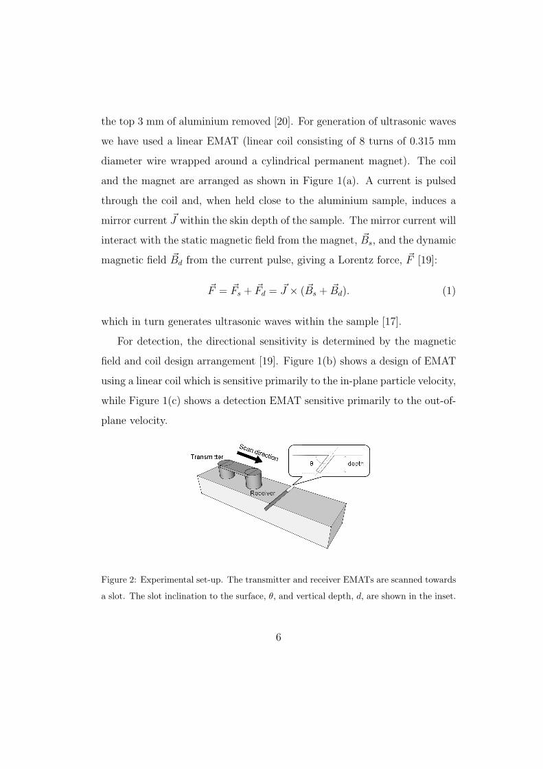
Figure 2: Experimental set-up. The transmitter and receiver EMATs are scanned towards
a slot. The slot inclination to the surface, θ, and vertical depth, d, are shown in the inset.
6
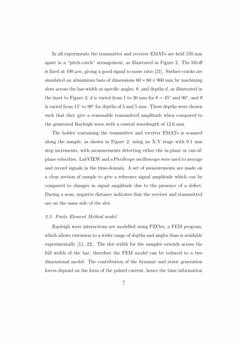
In all experiments the transmitter and receiver EMATs are held 150 mm
apart in a “pitch-catch” arrangement, as illustrated in Figure 2. The liftoff
is fixed at 100 µm, giving a good signal to noise ratio [21]. Surface cracks are
simulated on aluminium bars of dimensions 60× 60× 900 mm by machining
slots across the bar-width at specific angles, θ, and depths d, as illustrated in
the inset to Figure 2; d is varied from 1 to 20 mm for θ = 45◦ and 90◦, and θ
is varied from 15◦ to 90◦ for depths of 3 and 5 mm. These depths were chosen
such that they give a reasonable transmitted amplitude when compared to
the generated Rayleigh wave with a central wavelength of 12.6 mm.
The holder containing the transmitter and receiver EMATs is scanned
along the sample, as shown in Figure 2, using an X-Y stage with 0.1 mm
step increments, with measurements detecting either the in-plane or out-of-
plane velocities. LabVIEW and a PicoScope oscilloscope were used to average
and record signals in the time-domain. A set of measurements are made on
a clear section of sample to give a reference signal amplitude which can be
compared to changes in signal amplitude due to the presence of a defect.
During a scan, negative distance indicates that the receiver and transmitted
are on the same side of the slot.
2.2. Finite Element Method model
Rayleigh wave interactions are modelled using PZFlex, a FEM program,
which allows extension to a wider range of depths and angles than is available
experimentally [11, 22]. The slot width for the samples extends across the
full width of the bar, therefore the FEM model can be reduced to a two
dimensional model. The contribution of the dynamic and static generation
forces depend on the form of the pulsed current, hence the time information
7
from a measurement of the current is used to model the generation pulse.
The modelled sample has an element side length of 129µm, with the side
and bottom boundaries set as absorbing to minimise reflections. The slot
is defined as a rectangular void of 1 mm width, inclined at an angle θ and
depth d. 90◦, 45◦ and 22.5◦ slots are modelled with d ranging from 1 mm to
20 mm, while 3 mm and 5 mm slots were modelled with θ ranging from 15◦ to
165◦ at approximately 10◦ increments. The generation point has an effective
width of 2 mm and the in-plane and out-of-plane velocities are recorded at
each node from 150 mm to 250 mm away from the generation point.
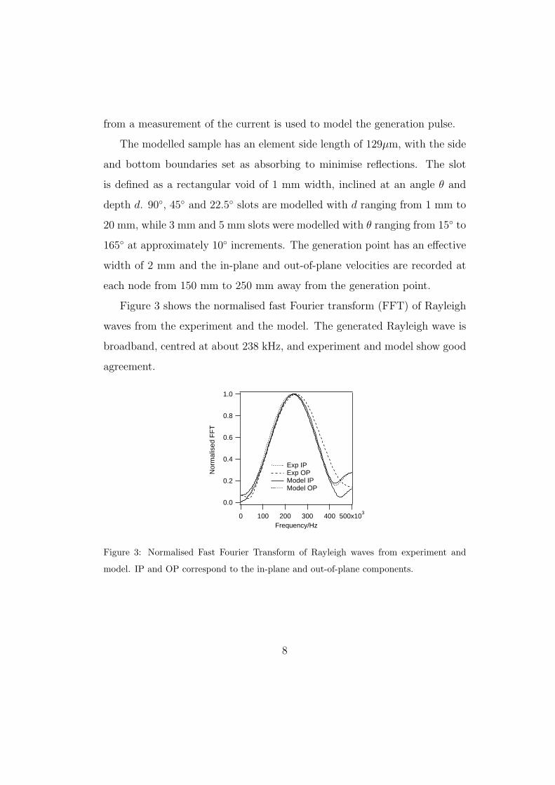
Figure 3 shows the normalised fast Fourier transform (FFT) of Rayleigh
waves from the experiment and the model. The generated Rayleigh wave is
broadband, centred at about 238 kHz, and experiment and model show good
agreement.
1.0
0.8
0.6
0.4
0.2
0.0
Nor
mal
ised
FF
T
500x103
4003002001000Frequency/Hz
Exp IP Exp OP Model IP Model OP
Figure 3: Normalised Fast Fourier Transform of Rayleigh waves from experiment and
model. IP and OP correspond to the in-plane and out-of-plane components.
8
2.3. Velocity components of the Rayleigh wave
EMATs are velocity sensors [19]. The particle velocities for a Rayleigh
wave in the in-plane, Vx, and out-of-plane, Vz, components can be calculated
from the displacements (Ux and Uz) given in Viktorov [5] as follows;
Vx = AωkR
(e−qz − 2qs
k2R + s2
e−sz
)cos(kRx− ωt) (2)
Vz = Aωq
(2k2
R
k2R + s2
e−sz − e−qz
)sin(kRx− ωt) (3)
where kR, kl and kt are the wave numbers of Rayleigh, longitudinal and shear
waves respectively, q =√
k2R − k2
l , s =√
k2R − k2
t , A is a constant and x and
z are the in-plane (x axis) and out-of-plane (z axis) positions.
1.0
0.5
0.0
-0.5
Nor
m. R
ayle
igh
velo
city
2.01.51.00.50.0Normalised depth, d/λ
Theory Model
In-plane
Out-of-plane (a)
-0.5
0.0
0.5
In-p
lane
to o
ut-o
f-pl
ane
ratio
2.01.51.00.50.0Normalised depth, d/λ
Theory Model
(b)
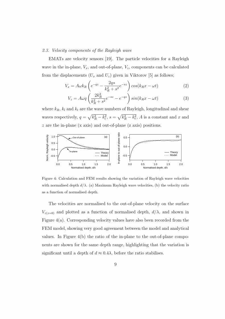
Figure 4: Calculation and FEM results showing the variation of Rayleigh wave velocities
with normalised depth d/λ. (a) Maximum Rayleigh wave velocities, (b) the velocity ratio
as a function of normalised depth.
The velocities are normalised to the out-of-plane velocity on the surface
Vz(z=0) and plotted as a function of normalised depth, d/λ, and shown in
Figure 4(a). Corresponding velocity values have also been recorded from the
FEM model, showing very good agreement between the model and analytical
values. In Figure 4(b) the ratio of the in-plane to the out-of-plane compo-
nents are shown for the same depth range, highlighting that the variation is
significant until a depth of d ≈ 0.4λ, before the ratio stabilises.
9
3. Experiment and FEM results
The analysis of each scan is divided into measurements in the far-field
and near-field regions of angled defects. Measurements of the transmission
are made in the far-field, where both EMATs are at least 5 wavelengths from
the slot (with the wavelength taken as the central wavelength, 12.6 mm).
At this distance the Rayleigh wave has stabilised following interaction with
the slot and the transmission coefficient can reliably be measured. Near-field
measurements are made when the receiver is very close to the slot, and signal
enhancement is observed [9, 10].
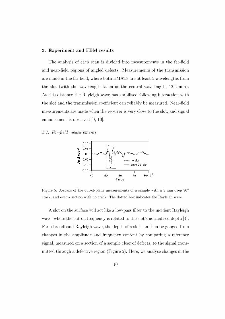
3.1. Far-field measurements
Figure 5: A-scans of the out-of-plane measurements of a sample with a 5 mm deep 90◦
crack, and over a section with no crack. The dotted box indicates the Rayleigh wave.
A slot on the surface will act like a low-pass filter to the incident Rayleigh
wave, where the cut-off frequency is related to the slot’s normalised depth [4].
For a broadband Rayleigh wave, the depth of a slot can then be gauged from
changes in the amplitude and frequency content by comparing a reference
signal, measured on a section of a sample clear of defects, to the signal trans-
mitted through a defective region (Figure 5). Here, we analyse changes in the
10
time-domain signals by measuring the peak-peak amplitude of the incident
(Ai) and transmitted (At) Rayleigh waves and calculating the transmission
coefficient, CT ,
CT =At
Ai
. (4)
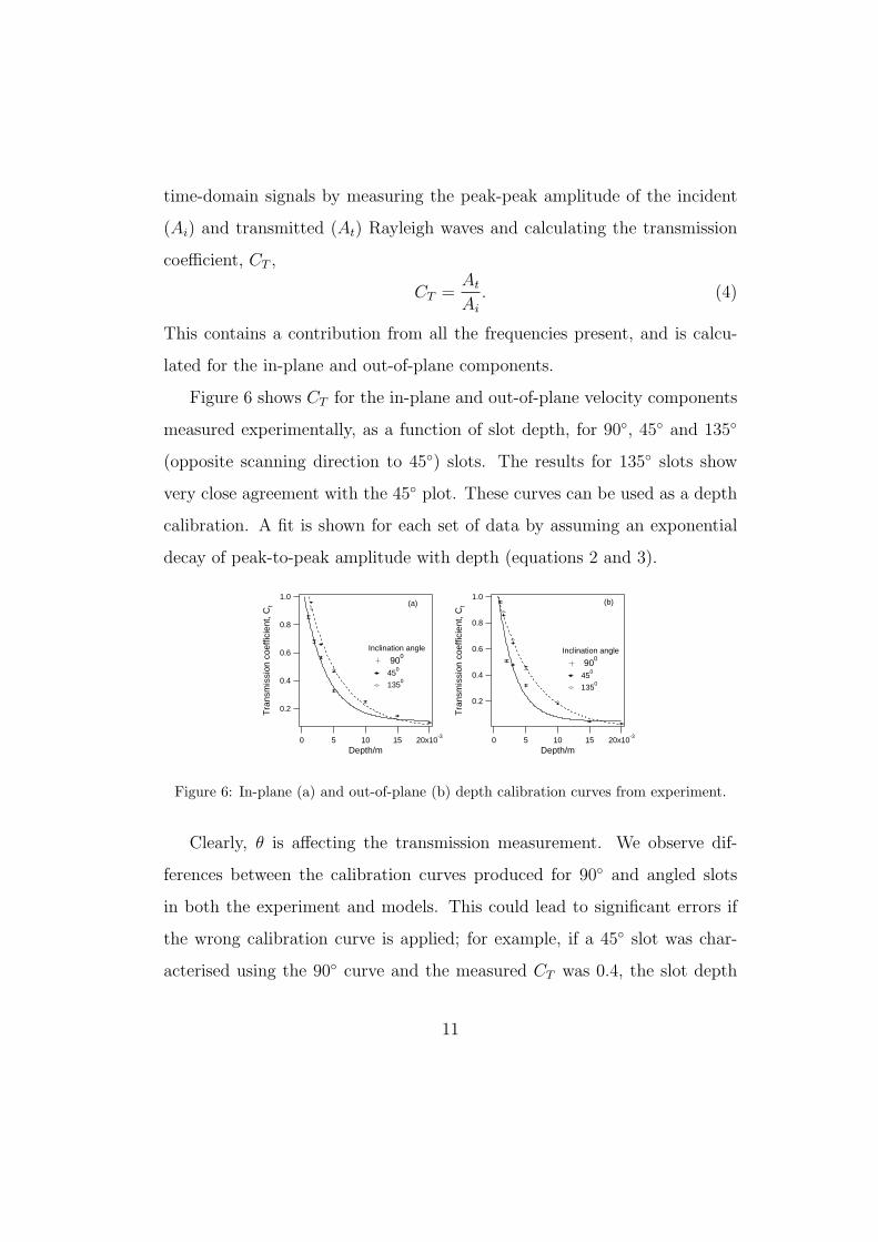
This contains a contribution from all the frequencies present, and is calcu-
lated for the in-plane and out-of-plane components.
Figure 6 shows CT for the in-plane and out-of-plane velocity components
measured experimentally, as a function of slot depth, for 90◦, 45◦ and 135◦
(opposite scanning direction to 45◦) slots. The results for 135◦ slots show
very close agreement with the 45◦ plot. These curves can be used as a depth
calibration. A fit is shown for each set of data by assuming an exponential
decay of peak-to-peak amplitude with depth (equations 2 and 3).
1.0
0.8
0.6
0.4
0.2Tra
nsm
issi
on c
oeffi
cien
t, C
t
20x10-3
151050Depth/m
Inclination angle
900
450
1350
(a)1.0
0.8
0.6
0.4
0.2
Tra
nsm
issi
on c
oeffi
cien
t, C
t
20x10-3
151050Depth/m
Inclination angle
900
450
1350
(b)
Figure 6: In-plane (a) and out-of-plane (b) depth calibration curves from experiment.
Clearly, θ is affecting the transmission measurement. We observe dif-
ferences between the calibration curves produced for 90◦ and angled slots
in both the experiment and models. This could lead to significant errors if
the wrong calibration curve is applied; for example, if a 45◦ slot was char-
acterised using the 90◦ curve and the measured CT was 0.4, the slot depth
11
would be underestimated by ≈ 2.3 mm. However, from the modelled results
the difference between the 22.5◦ and 45◦ calibration curves is very small. In
this case, a 22.5◦ slot can be characterised using the 45◦ calibration curve,
or vice versa. We cannot blindly rely on the 90◦ depth calibration curve to
accurately characterise all defects.
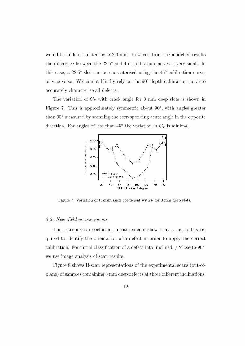
The variation of CT with crack angle for 3 mm deep slots is shown in
Figure 7. This is approximately symmetric about 90◦, with angles greater
than 90◦ measured by scanning the corresponding acute angle in the opposite
direction. For angles of less than 45◦ the variation in CT is minimal.
Figure 7: Variation of transmission coefficient with θ for 3 mm deep slots.
3.2. Near-field measurements
The transmission coefficient measurements show that a method is re-
quired to identify the orientation of a defect in order to apply the correct
calibration. For initial classification of a defect into ‘inclined’ / ‘close-to-90◦’
we use image analysis of scan results.
Figure 8 shows B-scan representations of the experimental scans (out-of-
plane) of samples containing 3 mm deep defects at three different inclinations,
12

θ = 22.5◦, 90◦ and 157.5◦. A-scans recorded at each position in a scan are
stacked together to form the B-scan, with the amplitudes of the waves given
by the colour scale. The y-axis shows the distance between the receive EMAT
and the slot, while the x-axis gives the arrival time, and each wave mode can
be identified by its arrival time as a function of scan position [11, 12, 14].
The incident Rayleigh wave arrives at about 52µs.
-15
-10
-5
0
5
10
15
Dis
t. of
rec
eive
r to
slo
t/mm
70x10-6
65605550Time/s
(a)
-15
-10
-5
0
5
10
15
Dis
t. of
rec
eive
r to
slo
t/mm
70x10-6
65605550Time/s
(b)
-15
-10
-5
0
5
10
15
Dis
t. of
rec
eive
r to
slo
t/mm
70x10-6
65605550Time/s
(c)
Figure 8: B-scans of the out-of-plane measurements showing the enhancement pattern
from 3 mm slots of inclinations (a) θ= 90◦, (b) θ= 22.5◦, (c) θ= 157.5◦.
There is a clear difference in the near-field between the scans. Firstly,
we can consider the changes in arrival time of a Rayleigh wave transmitted
underneath a defect. These have been calculated for incident, reflected and
transmitted Rayleigh waves, plus mode-converted bulk wavemodes, in [11,
12, 14], for normal and angled defects. For the 157.5◦ defect (Figure 8(c))
a significant delay in the Rayleigh wave arrival time is seen in the near-field
following transmission. This delay time is governed by the defect length and
inclination, and could be used for defect characterisation [23].
The enhancement pattern observed for each angle is also strikingly dif-
ferent, and can be used to position and characterise the defect. For a 90◦
slot this enhancement pattern is well understood; in Figure 8(a) the incident
and reflected Rayleigh waves can be seen interfering constructively close to
the defect (with a surface skimming longitudinal wave contributing signifi-
13
cantly to the in-plane enhancement [10]). However, in Figures 8(b) & (c) the
signal enhancement is stronger and has a different time dependence, forming
an alternating black and white pattern. The pattern produced by the 90◦
slot extends to about 58 µs, while the 22.5◦ slot produces an enhancement
pattern that spans to the end of the time scale shown. Furthermore, the
enhancement has a clear dependence on angle.
Image analysis of these B-scans gives some information about the defect.
Firstly, the position of the slot can be determined from the enhancement.
Secondly, a distinction between near-90◦ slots and inclined slots can be made.
Finally, the orientation of the slot tip, i.e. whether it is facing (acute angle) or
opposing (obtuse angle) the direction of travel of the incident Rayleigh wave
can be determined. An image classification program using machine learning
has been developed to extract this information from a B-scan, with initial
results giving a 100% accuracy in identification for a small data set [24].
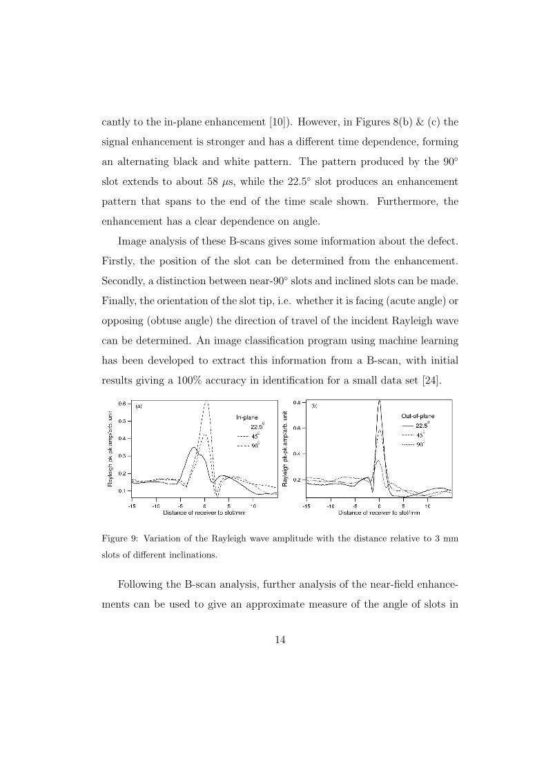
Figure 9: Variation of the Rayleigh wave amplitude with the distance relative to 3 mm
slots of different inclinations.
Following the B-scan analysis, further analysis of the near-field enhance-
ments can be used to give an approximate measure of the angle of slots in
14
the range 0◦ 6 θ 6 90◦. To quantify the enhancement the peak-to-peak
amplitude of the Rayleigh wave is measured at each scan point and plotted
as a function of scan distance, as shown in Figure 9 for 3 mm deep slots. A
new parameter, the enhancement factor FE, is introduced as the measure of
the enhancement, by normalising the enhanced amplitude, AE, at the peak
by the reference amplitude Ai;
FE =AE
Ai
. (5)
FE is calculated for both the in-plane and out-of-plane measurements,
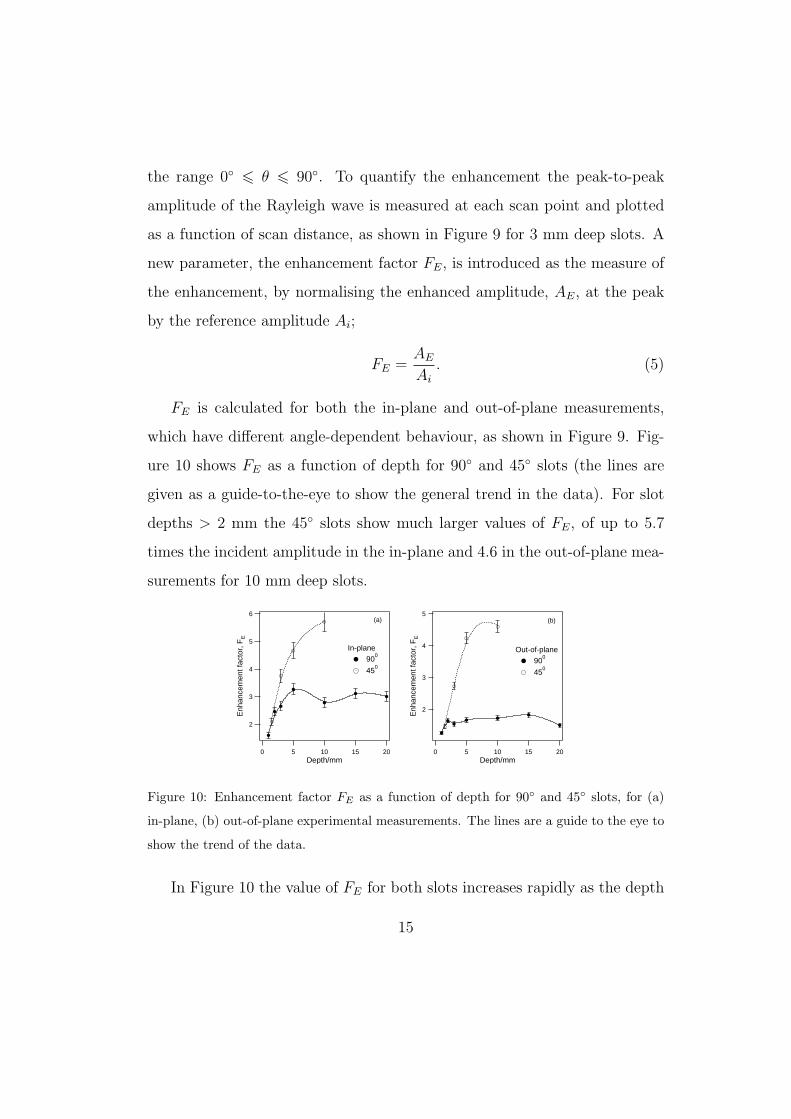
which have different angle-dependent behaviour, as shown in Figure 9. Fig-
ure 10 shows FE as a function of depth for 90◦ and 45◦ slots (the lines are
given as a guide-to-the-eye to show the general trend in the data). For slot
depths > 2 mm the 45◦ slots show much larger values of FE, of up to 5.7
times the incident amplitude in the in-plane and 4.6 in the out-of-plane mea-
surements for 10 mm deep slots.
6
5
4
3
2
Enh
ance
men
t fac
tor,
FE
20151050Depth/mm
In-plane 90
0
450
(a)5
4
3
2
Enh
ance
men
t fac
tor,
FE
20151050Depth/mm
Out-of-plane 90
0
450
(b)
Figure 10: Enhancement factor FE as a function of depth for 90◦ and 45◦ slots, for (a)
in-plane, (b) out-of-plane experimental measurements. The lines are a guide to the eye to
show the trend of the data.
In Figure 10 the value of FE for both slots increases rapidly as the depth
15
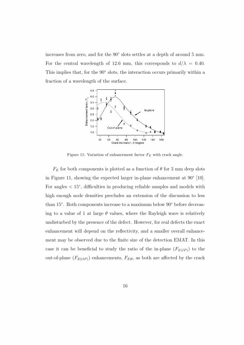
increases from zero, and for the 90◦ slots settles at a depth of around 5 mm.
For the central wavelength of 12.6 mm, this corresponds to d/λ = 0.40.
This implies that, for the 90◦ slots, the interaction occurs primarily within a
fraction of a wavelength of the surface.
Figure 11: Variation of enhancement factor FE with crack angle.
FE for both components is plotted as a function of θ for 3 mm deep slots
in Figure 11, showing the expected larger in-plane enhancement at 90◦ [10].
For angles < 15◦, difficulties in producing reliable samples and models with
high enough node densities precludes an extension of the discussion to less
than 15◦. Both components increase to a maximum below 90◦ before decreas-
ing to a value of 1 at large θ values, where the Rayleigh wave is relatively
undisturbed by the presence of the defect. However, for real defects the exact
enhancement will depend on the reflectivity, and a smaller overall enhance-
ment may be observed due to the finite size of the detection EMAT. In this
case it can be beneficial to study the ratio of the in-plane (FE(IP )) to the
out-of-plane (FE(OP )) enhancements, FER, as both are affected by the crack
16

characteristics;
FER =FE(IP )
FE(OP )
. (6)
This ratio was calculated and plotted as a function of θ for slots of vertical
depth 3 mm and 5 mm for both model and experiment, shown in Figure 12.
A dashed line is given as a guide to the eye, but is not intended to be an
accurate fit. The plot shows that the FER values are less than 1 in the small
angle region (15◦-35◦) and increase gradually above 1 for angles greater than
45◦; the out-of-plane component is found to be more dominant than the in-
plane in the small angle region, while the opposite is true outside this range.
Figure 12: Variation of enhancement factor ratio, FER with crack inclination, θ. The
dashed line is a guide to the eye only.
In order to understand this behavior, one can first consider the behaviour
of Rayleigh waves incident on a wedge [25, 26]. Within the wedge the local
thickness varies depending on the position relative to the tip. As the Rayleigh
wave here interacts with an angled defect, some of the wave will be trans-
mitted underneath the slot, while the rest will be trapped within the wedge
formed by the defect. Considering the change of the frequency-thickness,
from the full bar thickness to the local thickness within the angled defect,
17
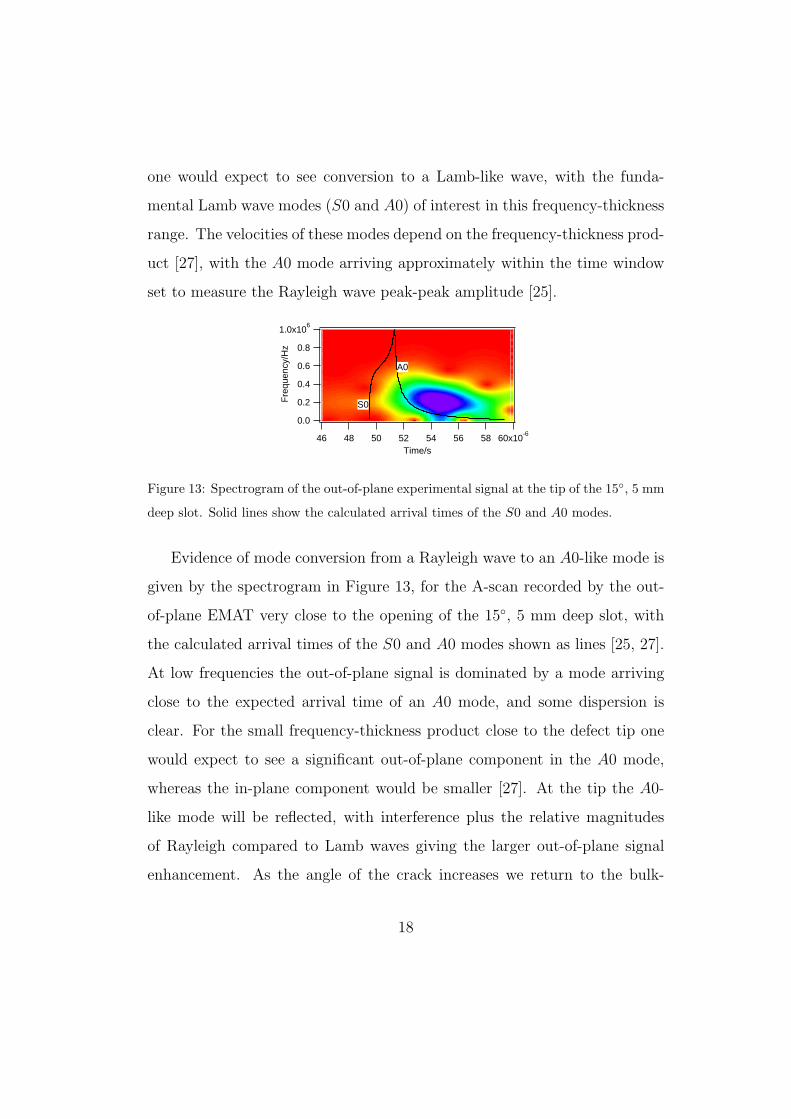
one would expect to see conversion to a Lamb-like wave, with the funda-
mental Lamb wave modes (S0 and A0) of interest in this frequency-thickness
range. The velocities of these modes depend on the frequency-thickness prod-
uct [27], with the A0 mode arriving approximately within the time window
set to measure the Rayleigh wave peak-peak amplitude [25].
1.0x10⁶
0.8
0.6
0.4
0.2
0.0
Fre
quen
cy/H
z
60x10-6
58565452504846Time/s
A0
S0
Figure 13: Spectrogram of the out-of-plane experimental signal at the tip of the 15◦, 5 mm
deep slot. Solid lines show the calculated arrival times of the S0 and A0 modes.
Evidence of mode conversion from a Rayleigh wave to an A0-like mode is
given by the spectrogram in Figure 13, for the A-scan recorded by the out-
of-plane EMAT very close to the opening of the 15◦, 5 mm deep slot, with
the calculated arrival times of the S0 and A0 modes shown as lines [25, 27].
At low frequencies the out-of-plane signal is dominated by a mode arriving
close to the expected arrival time of an A0 mode, and some dispersion is
clear. For the small frequency-thickness product close to the defect tip one
would expect to see a significant out-of-plane component in the A0 mode,
whereas the in-plane component would be smaller [27]. At the tip the A0-
like mode will be reflected, with interference plus the relative magnitudes
of Rayleigh compared to Lamb waves giving the larger out-of-plane signal
enhancement. As the angle of the crack increases we return to the bulk-
18
wave picture close to 90◦, with enhancement again mainly due to interference
of incident and reflected Rayleigh waves with the mode-converted surface
skimming longitudinal mode, with the in-plane enhancement dominating.
Comparing measured values of FER to the calibration in Figure 12 will
give an approximate value of θ to within about 10◦. The estimate is sufficient
to give the correct depth calibration curve to use for a depth measurement.
4. Procedure for characterising surface cracks
In this section we describe a procedure (Figure 14) which has been devel-
oped to use the far-field and near-field measurements to characterise surface
cracks, finding their vertical depth, orientation of the crack (i.e. whether the
crack tip is facing the incoming Rayleigh wave or opposing it), and a rough
estimate of the crack angle to the surface. The scan of the sample, which can
either be done separately for the in-plane and out-of-plane measurements, or
by using a trolley holding two receiver EMATs, is set such that the receiver
will be initially in the far-field, is then scanned over a crack (near-field) and
then reaches the far-field region on the other side of the crack. From the scan,
several analyses are done in parallel; B-scan analysis (image analysis), and
Rayleigh wave peak-peak amplitude analysis in both the near (enhancement)
and far-field (transmission) regions.
The B-scan analysis gives the position of the crack, along with an indica-
tion of whether the crack is in the near-90◦ range or inclined to the surface.
For a near-90◦ crack, the depth estimate can be done directly from CT , with
characterisation using the 90◦ depth calibration curve (Figure 6). For inclined
cracks, we first determine the orientation of the crack using the B-scan. If
19
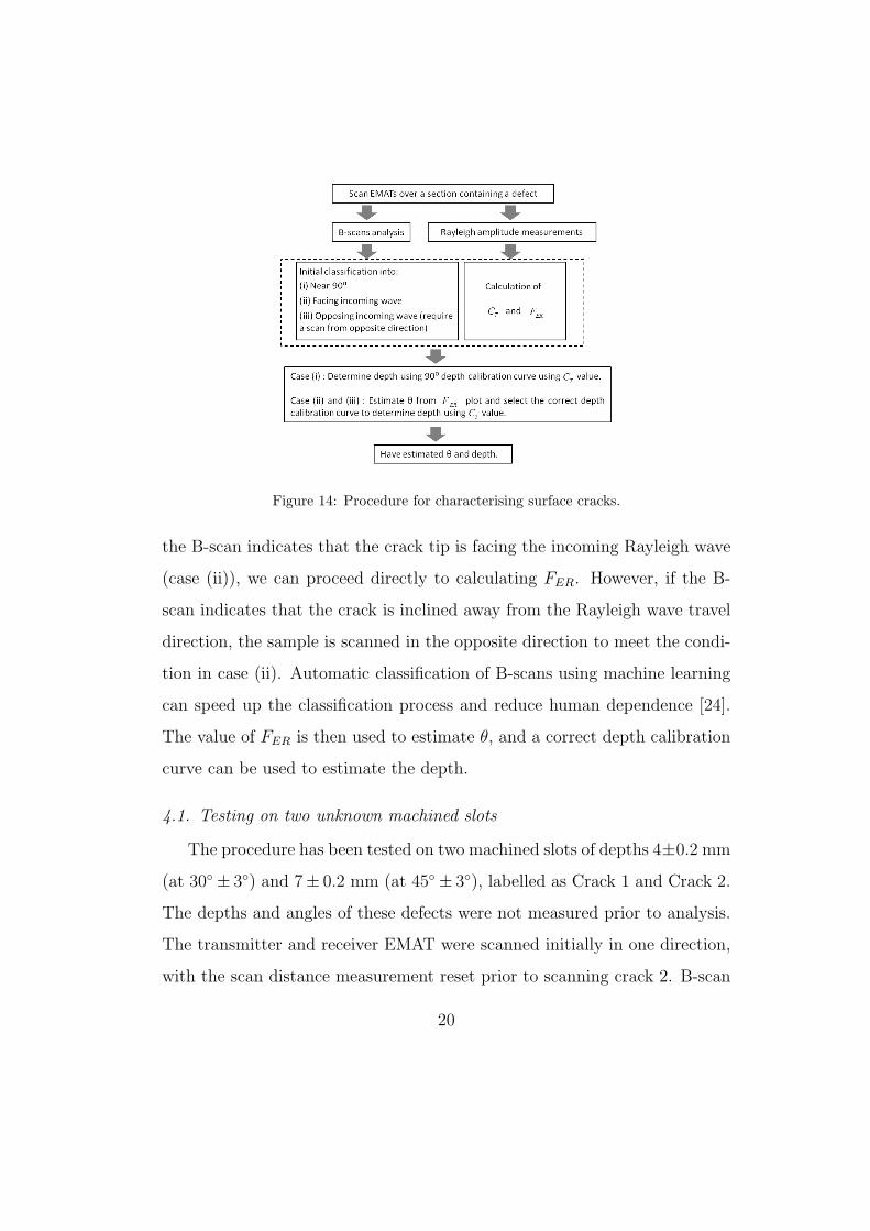
Figure 14: Procedure for characterising surface cracks.
the B-scan indicates that the crack tip is facing the incoming Rayleigh wave
(case (ii)), we can proceed directly to calculating FER. However, if the B-
scan indicates that the crack is inclined away from the Rayleigh wave travel
direction, the sample is scanned in the opposite direction to meet the condi-
tion in case (ii). Automatic classification of B-scans using machine learning
can speed up the classification process and reduce human dependence [24].
The value of FER is then used to estimate θ, and a correct depth calibration
curve can be used to estimate the depth.
4.1. Testing on two unknown machined slots
The procedure has been tested on two machined slots of depths 4±0.2 mm
(at 30◦ ± 3◦) and 7± 0.2 mm (at 45◦ ± 3◦), labelled as Crack 1 and Crack 2.
The depths and angles of these defects were not measured prior to analysis.
The transmitter and receiver EMAT were scanned initially in one direction,
with the scan distance measurement reset prior to scanning crack 2. B-scan
20
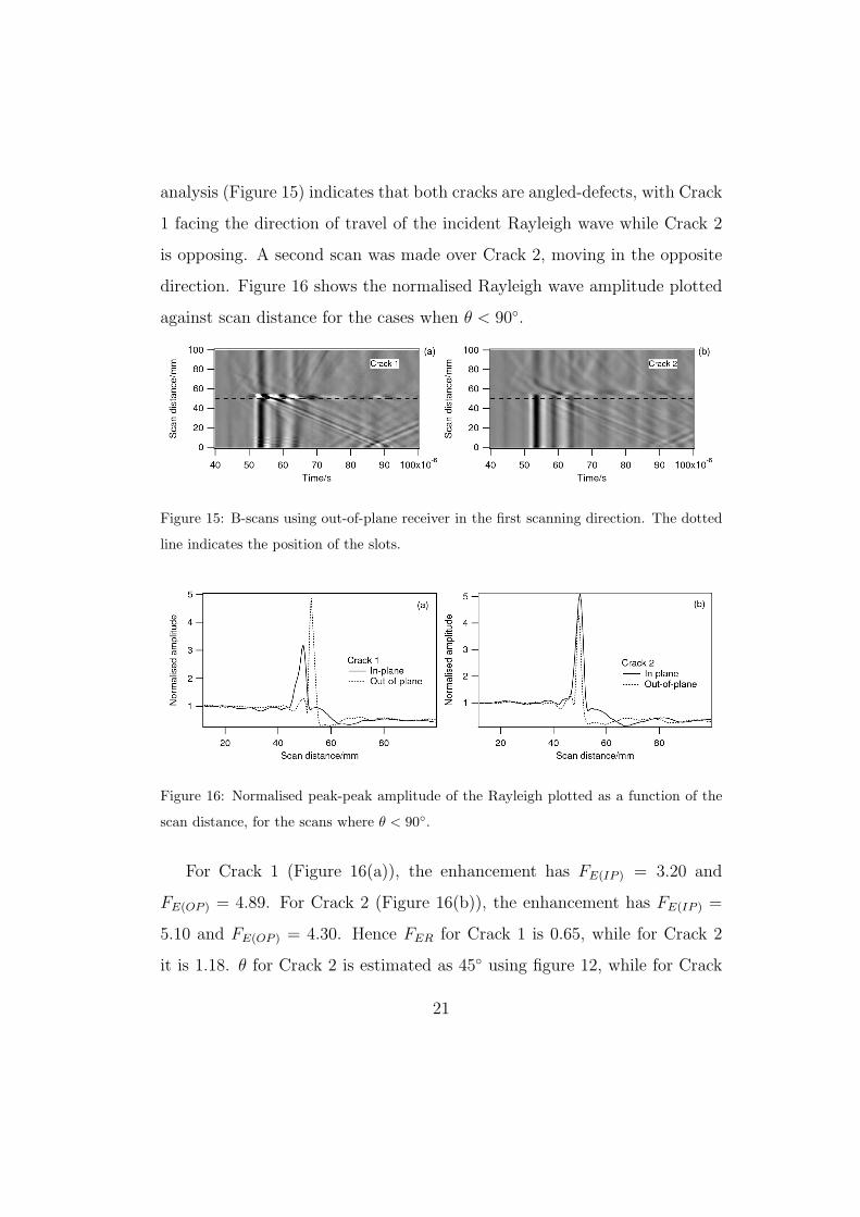
analysis (Figure 15) indicates that both cracks are angled-defects, with Crack
1 facing the direction of travel of the incident Rayleigh wave while Crack 2
is opposing. A second scan was made over Crack 2, moving in the opposite
direction. Figure 16 shows the normalised Rayleigh wave amplitude plotted
against scan distance for the cases when θ < 90◦.
Figure 15: B-scans using out-of-plane receiver in the first scanning direction. The dotted
line indicates the position of the slots.
Figure 16: Normalised peak-peak amplitude of the Rayleigh plotted as a function of the
scan distance, for the scans where θ < 90◦.
For Crack 1 (Figure 16(a)), the enhancement has FE(IP ) = 3.20 and
FE(OP ) = 4.89. For Crack 2 (Figure 16(b)), the enhancement has FE(IP ) =
5.10 and FE(OP ) = 4.30. Hence FER for Crack 1 is 0.65, while for Crack 2
it is 1.18. θ for Crack 2 is estimated as 45◦ using figure 12, while for Crack
21
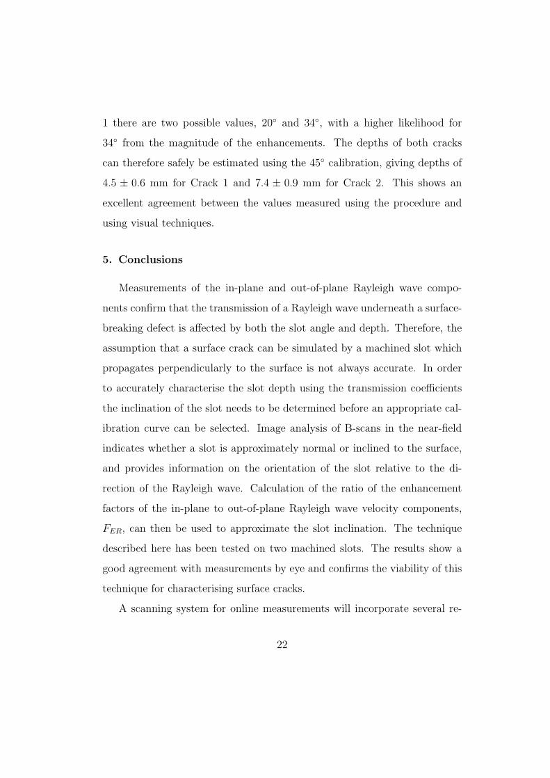
1 there are two possible values, 20◦ and 34◦, with a higher likelihood for
34◦ from the magnitude of the enhancements. The depths of both cracks
can therefore safely be estimated using the 45◦ calibration, giving depths of
4.5 ± 0.6 mm for Crack 1 and 7.4 ± 0.9 mm for Crack 2. This shows an
excellent agreement between the values measured using the procedure and
using visual techniques.
5. Conclusions
Measurements of the in-plane and out-of-plane Rayleigh wave compo-
nents confirm that the transmission of a Rayleigh wave underneath a surface-
breaking defect is affected by both the slot angle and depth. Therefore, the
assumption that a surface crack can be simulated by a machined slot which
propagates perpendicularly to the surface is not always accurate. In order
to accurately characterise the slot depth using the transmission coefficients
the inclination of the slot needs to be determined before an appropriate cal-
ibration curve can be selected. Image analysis of B-scans in the near-field
indicates whether a slot is approximately normal or inclined to the surface,
and provides information on the orientation of the slot relative to the di-
rection of the Rayleigh wave. Calculation of the ratio of the enhancement
factors of the in-plane to out-of-plane Rayleigh wave velocity components,
FER, can then be used to approximate the slot inclination. The technique
described here has been tested on two machined slots. The results show a
good agreement with measurements by eye and confirms the viability of this
technique for characterising surface cracks.
A scanning system for online measurements will incorporate several re-
22
ceive EMATs, giving both in-plane and out-of-plane measurements in a single
scan, so that information from both can be acquired in parallel. Provided
that a preliminary reference measurement is made over an clear section of
the sample, analysis can be done during a scan to produce a real-time char-
acterisation of surface cracks.
Acknowledgments This work was funded by the European Research Coun-
cil under grant 202735, ERC Starting Independent Researcher Grant. We
also thank NESTA for Crucible Seed Funding.
References
[1] R.A. Cottis, Guides to Good Practice in Corrosion Control: Stress Cor-
rosion Cracking, HMSO (2000)
[2] Railtrack Plc., Rolling Contact Fatigue in Rails; A Guide to Current
Understanding and Practice (2001)
[3] D. Hesse and P. Cawley, Review of Progress in Quantitative Nonde-
structive Evaluation 25A&B (AIP Conference Proceedings Vol. 820)
1593-1600 (2006)
[4] R.S. Edwards, S, Dixon and X. Jian, Ultrasonics 44(1) 93-98 (2006)
[5] I.A. Viktorov, Rayleigh Waves and Lamb Waves-Physical Theory and
Application, Plenum Press, New York (1967)
[6] D.A. Mendelsohn, J.D. Achenbach and L.M. Keer, Wave Motion 2(3)
277-292 (1980)
23
[7] R.S. Edwards, S. Dixon and X. Jian, NDT & E International 39(6)
468-475 (2006)
[8] S. Dixon, B. Cann, D.L. Carroll, Y. Fan and R.S. Edwards, Nondestruc-
tive Testing and Evaluation 23(1) 25-34 (2008)
[9] J.L Blackshire and S. Sathish, Applied Physics Letters 80(18) 3442-3444
(2002)
[10] R.S. Edwards, X. Jian, Y. Fan and S. Dixon, Applied Physics Letters
87(19) 194104 (2005)
[11] X. Jian, S. Dixon, N. Guo and R. Edwards, Journal Of Physics D -
Applied Physics 101(6) 064906 (2007)
[12] B. Dutton, A.R. Clough, M.H. Rosli and R.S. Edwards, NDT & E In-
ternational 44(4) 353-360 (2011)
[13] V.K. Kinra and B.Q. Vu, Journal of the Acoustical Society of America
79(6) 1688-1692 (1986)
[14] C.Y. Ni, Y.F. Shi, Z.H. Shen, J.A. Lu and X.W. Ni, NDT&E Interna-
tional 43(6) 470-475 (2010)
[15] I. Baillie, P. Griffith, X. Jian and S. Dixon, Review Of Progress In Quan-
titative Nondestructive Evaluation 28A&B (AIP Conference Proceed-
ings Vol. 1096) 1711-1718 (2009)
[16] A. Moura, A.M. Lomonosov and P. Hess, Journal of Applied Physics
103(8) 084911 (2008)
24

[17] S.B. Palmer and S. Dixon, Insight 45(3) 211-217 (2003)
[18] M. Hirao and H. Ogi, EMATs for Science and Industry, Kluwer Aca-
demic Publishers (2003)
[19] X. Jian, S. Dixon, K. Quirk and K.T.V. Grattan, Sensors & Actuators
A - Physical 148(1) 51-56 (2008)
[20] S. Dixon, C. Edwards and S.B. Palmer, Insight 40(9) 632-634 (1998)
[21] J.P. Morrison, S. Dixon, M.D.G. Potter and X. Jian, Ultrasonics 44
E1401-E1404 (2006)
[22] X. Jian, Y. Fan, R.S. Edwards and S. Dixon, Journal of Applied Physics
100(6) 064907 (2006)
[23] A.R. Clough, B. Dutton and R.S. Edwards, Review Of Progress In Quan-
titative Nondestructive Evaluation 30A&B 137-144 (2011)
[24] M.H. Rosli, R.S. Edwards, B. Dutton, C.G. Johnson and P.T. Cattani,
Review Of Progress In Quantitative Nondestructive Evaluation 29A&B
(AIP Conference Proceedings Vol. 1211) 1593-1600 (2010)
[25] R.S. Edwards, B. Dutton, A.R. Clough and M.H. Rosli, Applied Physics
Letters 99(9) 094104 (2011)
[26] R.J. Blake and L.J. Bond, Ultrasonics 28(4) 214-228 (1990)
[27] J.L. Rose, Ultrasonic Waves in Solid Media, Cambridge University
Press(1999)
25