To invited reader

1

To invited reader:

Many thanks for your comments and suggestions on my paper. I have incorporated with the comments

and suggestions in the following revised version. One of the highlights in this revised version is

subsection “1.4 Critical investigations to revealed preference theory” that reveals revealed preference

theory meaningless as a positive description (see pp. 7~11).

For the convenient reading, all revised parts have been blue-colored in the text, and the intensively

revised page numbers and contents are specified below. Indeed, I would like to hear from you again.

1. pp. 4-5

“Introduction” has been rewritten to clearly describe what the paper actually does and what it tries to

achieve.

2. pp. 5~11

The section “1 Analytical path” has been wholly rewritten and the psychophysical approach,

Klein-Rubin utility function, and Linear Expenditure System are described in detail. Especially, it also

highlights on the critical analysis on revealed preference theory. This section consists of four

subsections “1.1”~“1.4” that are specified as the following:

(1) p. 6: “1.1 Economic Attribute of Klein-Rubin utility function”. It explains the economics

foundation for Klein-Rubin utility function and the derivation for LES.

(2) pp. 6~7: “1.2 Psychological attribute of Klein-Rubin utility function”. It explains the

psychophysical measurements for Klein-Rubin utility function.

(3) p. 7: “1.3 Comparison between ULES and UEst”. It explains how to test utility maximization

hypothesis in this paper.

(4) pp. 7~11: “1.4 Critical investigations to revealed preference theory”. In this subsection, a critical

analysis on revealed preference theory reveals that revealed preference theory is only

meaningful as a normative system but meaningless as a positive description, and the

existing experimental and empirical verifications for utility maximization in revealed

preference theory are wholly invalid.

3. pp. 13~14

“2.1.2 Session B in Exp. 1” is rewritten with more detailed and comprehensible contents.

4. p. 15

The explanation is improved to describe how to discriminate “a purely exhausting consumer” in

Choices I~III.

5. p. 17

“Fig 1” is added to illustrate the bid price inquiry card used in Session B of Exp.1.

2

6. p. 23

“Fig 2” is added to illustrate the changed bid price inquiry card that may be used in Session B of Exp.1.

7. pp. 24~25

New contents are added to explain the necessity of discriminating the perception utility and emotion

utility.

8. Other questions addressed in your report are replied here:

(1) About the instructions used in the experiment

They are presented on p.15 (the top paragraph), p.15 (the bottom paragraph), and p.17 (the bottom

paragraph).

(2) About “only a minority of the subjects seem to have completed the experiments”

The subjects participating in the experiments were not previously selected, and their preferences to

three kinds of kernels could be very different. The most popular three groups that delivered invalid data

were, first, those who did not choose all three kernels in Choice I violating Valid Condition 4 (see the

second paragraph from the bottom on p.15) for they disliked certain kernels, second, those who were

judged as “purely exhausting consumers” violating Valid Condition 2 (see the bottom paragraph on

p.12 and the second paragraph on p.13; for the notion of “purely exhausting consumers” please see the

subsection “1.4” on pp.7~11), and, third, those who purchased below RMB3.00 in Exp. 1 or below

RMB3.60 in Exp. 2 violating Valid Condition 1 (see the second paragraph from the bottom on p.12 and

the fourth paragraph on p.18). In the total invalid number for all formal experiments, the first group

occupied a proportion about 50%, the second about 26%, and the third about 20%. All those invalid

determinants are uncontrollable in subjects’ behaviors, and it is evidently more reasonable to pick them

out in the experiments than previously to rule them out before the experiments.

(3) About “why this is a cardinal utility test”

The psychophysical measures to the utility scales for UEst are the cardinal measure (see He, 2012), so it

is a cardinal utility test. Also see the third paragraph on p.5, the third paragraph from the bottom on p.7.

3

Experimental Test of Utility Maximization

Yuqing He

Jinan University

Abstract: The study tested the cardinal utility maximization hypothesis by an experimental procedure

in a framework of utility scaling approach following the psychophysics-econometrics paradigm,

conceived in He (Psychophysical Interpretation for Utility Measures, 2012). It reveals (i) the cardinal

utility maximization can be tested and has been supported by experimental results; (ii) the utility

scaling approach following the psychophysics-econometrics paradigm offers a new foundation to

discuss the utility concept; and (iii) it is necessary to distinguish the perception utility and emotion

utility to respectively describe economic choices and enjoyment choices. A critical analysis on revealed

preference theory is also highlighted, and it discloses revealed preference theory only meaningful as a

normative system but not as a positive description.

JEL A10, D01

Keywords utility maximization; experiment; Klein-Rubin utility function; revealed preference;

perception utility; emotion utility

Correspondence Department of Public Administration, Jinan University, Guangzhou 510632,

Guangdong Province, China; E-mail: hyq5.27@163. com

4

Introduction

If give a survey over the cardinal utility researches after 1960s, you certainly see that the cardinal

utility is not as immeasurable as it had been pessimistically thought during the first half of 20th century.

The successful psychophysical studies appealing us to attempt the cardinal utility measurement as a

sensation scaling had appeared for a long time (e.g., Galanter, 1962, 1990; Galanter and Pliner, 1974;

Galanter et al., 1977; Breaut, 1983; Parker and Schneider, 1988). A number of experimental and

theoretical studies have systematically revealed the cardinal utility measurable for both commodity

choice and risk choice (e.g., Tversky and Kahneman, 1992; Gonzalez and Wu, 1999; He, 2012). The

base for laying out the utility theory has changed today and far differs from the times of ordinalist and

revealed-preferencian pioneers or leading founders Pareto (1906), Johnson (1913), Frisch (1926),

Hicks and Allen (1934), Alt (1936), and Samuelson (1938). Mainstream economics might neglect such

a historical change for too long a time. This change naturally reignited a debate between cardinal utility

and ordinal utility or revealed preference theories (e.g., Kahneman et al., 1997; He, 2012). It is

necessary to clarify this debate before an experimental test of cardinal utility maximization can be well

reasonably carried on. A critical investigation for it will be presented in Subsection 1.4.

There have been three paths presented in the literature for using data to study the utility

maximization: cardinal measure, revealed preference measure, and econometric modeling approach.

This paper will combine the cardinal measure with the econometric modeling approach to carry on the

experimental test of utility maximization in a psychophysics-econometrics paradigm, proposed in He,

2012.

Indeed, revealed preference theory claims its success in testing the utility maximization hypothesis

only by the comparisons between consumers or subjects’ choices at different budget levels (e.g. Varian,

1982, 1983, 2009). That will be cleared up in Subsection 1.4 as a misunderstanding. Here we focus on

the relationship between cardinal utility measure and econometric modeling approach.

Conventional cardinal utility measure came from Bentham tradition, following the hedonic

interpretation for economic utility and often leading to psychological discussions today. Econometric

modeling approach bases on the general statistical framework or utility maximization framework, and

this paper will follow the latter, which belongs to marginal analysis tradition and always reveals

parametric relationships fitted to empirical observations. The cardinal utility measure and the

econometric modeling approach had always been departed from one another in the history. To clarify

the isolation between them, it is helpful to briefly review the earlier utility thoughts.

The modern utility thought originated from Bentham’s nominal measures of pleasure, happiness,

and etc (Bentham, 1789). Bentham’s outstanding contribution to the utility theory was to make the

utility concept be viewed as a numerical magnitude, not by any successful measurement but by

repeated fruitless discussions (e.g. Stigler, 1950). If no utility maximization hypothesis jointed since

Gossen (1854), the utility thought would stay mainly as an academic language decoration and would

never become one of core thoughts in economics. It was the utility maximization reasoning to combine

the nominal hedonic measures deeply with the marginal analysis and to root the utility discussion

deeply into economics. It changed the language of utility analysis into a more precise, complicated, and

abstruse natural science form in its reasoning aspect, but in its pioneering era, never approached to

another characteristic of natural science: test a hypothesis in the experiment. The relationship between

the hedonic concept of economic utility and the utility maximization in econometric models has never

been verified by any empirical or experimental observations, and it is only a preconception inherited

5

from Bentham.

For a long time, the utility maximization analysis was departed into two isolate domains in the

cardinal utility exploration: one is the experimentation that concerns with the psychological hedonic

aspect and terminates to change non-quantitative intuitive hedonic experiences into quantitative

psychological analyses (e.g., Breaut, 1983; Kahneman et al., 1997), related to Bentham’s tradition; and

the other is the econometrics that concerns with the economic money aspect and starts from theoretical

construction of utility function to explore the utility maximization model for describing market

monetary distribution behaviors (e.g., Klein and Rubin, 1947; Stone, 1954; Liuch, 1973; Houthakker,

1960; Theil, 1965; Deaton and Muellbauer, 1980), related to the marginal analysis tradition. For

experimentalists the utility seems a hedonic feeling somehow to relate with the money distribution in

one’s economic concern, while, for econometricians the utility is only a mathematical function “u”,

which can be maximized, somehow to involve one’s hedonic feelings. This is of the realistic pictures

for the utility research differently between experimentalists and econometricians. Such a demarcation

cut the complete utility maximization issue into two irrelevant halves, and made either experimentation

or modeling approach fail to deal with a complete behavioral process in the utility maximization. It

truly disabled the test of cardinal utility maximization.

He, 2012 has theoretically and experimentally verified that the maximized Klein-Rubin utility

function (Klein and Rubin, 1947; Geary, 1950) in econometric model Linear Expenditure System (LES)

(Stone, 1954) is the linear combination of subjective quantities of commodities, derived from one’s

cardinal sensation response rather than Bentham’s emotional measures. That is, utility is a cardinal

sensation measure to the commodity quantity when it is maximized in an econometric model.

Miscomprehending the maximized utility as Bentham’s hedonic one is a substantial barrier isolating the

cardinal utility measure from the econometric modeling approach.

We have cleared away the obstacles and paved the way for the combination of cardinal utility

measure and econometric modeling approach to experimentally test the utility maximization hypothesis

in a framework associating sensation scaling in commodity choices with parametric estimation in the

econometric model. We have come to a time to relook at the cardinal utility maximization hypothesis

through the experimental insight.

Section 1 describes the rationale underlying this study, and it will also highlight on a critical

investigation to revealed preference theory. Section 2 will report in detail how such a test was designed

and had been performed in an experimental procedure during March and April, 2012. And Section 3

presents the experimental results.

This study revealed that the cardinal utility maximization holds in subjects’ choice behaviors in a

three-commodity bundle at the acceptable level of R2 ≥ 0.97 for the curve fitting. Waiting for one

hundred and fifty-eight years, Gossen’s genius is firstly supported by experimental evidences. More

important for resent economics, such an experimental study indicates a new analytical framework for

economics, which will be discussed in Section 4 that also summarizes and discusses the findings.

The data sets and appended mathematical derivations are presented in Supplemental Files on the

journal’s web site http://hdl.handle.net/1902.1 /18501.

1 Analytical path

There are two experimental ways to independently determine a Klein-Rubin utility function. One is to

solve LES in experimental data for the Klein-Rubin utility function. Another, proposed in He, 2012, is

6

to estimate the utility scales for respective commodities by psychophysical measures, then put them

into a linear combination to derive a Klein-Rubin utility function. The former utilizes the economic

attribute of the Klein-Rubin utility function, and the latter the psychological attribute of the

Klein-Rubin utility function. The present experimental test of utility maximization will be realized

through a comparison between the Klein-Rubin utility functions obtained from the two ways.

On the other hand, following Afriat (1967) and Varian (1982)’s conceptions, revealed preference

theory had stepped into the same issue in its own comprehension. We shall inevitably encounter the

disputation between cardinal utility description and revealed preference theory in this section.

1.1 Economic Attribute of Klein-Rubin utility function

Satisfying the following three constraints in the consumer theory:

1) Budget constraint

eqpn

iii =∑

=1

,

2) Utility maximization condition

n

n

p

qu

p

qu

p

qu

∂∂

==∂∂

=∂∂

L

2

2

1

1 ,

and 3) Slutsky equation

iji

jj

i se

qq

p

q+

∂∂

−=∂∂

，

a utility function U describing consumer’s choices in an n-commodity bundle, called Klein-Rubin

utility function, is derived as

)ln( iii rqbU −=∑ , i=1,2,3,…,n,

where ri is the constant for commodity i, ∑ −

−=

)(

)(

imii

imiii

rqp

rqpb , and qmi, i=1.2.3….,n, is the quantities

maximizing utility U (Klein and Rubin, 1947; Geary, 1950) .

By maximizing the Klein-Rubin utility function in Lagrange’s approach, an econometric model

called Linear Expenditure System (LES) can be obtained (Stone, 1954):

)(11∑∑==

−+=n

iii

n

iiiiiiii rpqpbrpqp , i=1,2,3,…,n.

LES is a multi-equation system, can be solved in empirical data, and has been a fruitful theoretical

model describing consumers’ commodity purchases in numerous empirical statistics (e.g., see

Intriligator, 1980). Following its successful applications in the empirical study, we will utilize LES to

the experimental quantity choices qi in a commodity bundle with assigned prices pi. By solving LES for

bi and ri in experimental data of pi and qi, the Klein-Rubin utility function will be determined for

experimental samples. Below, denote ULES as the Klein-Rubin utility function experimentally derived

from LES.

LES is the result of maximizing the Klein-Rubin utility function, and thus, ULES is the utility

function theoretically required by the utility maximization for the chosen commodity bundle in the

experiment.

1.2 Psychological attribute of Klein-Rubin utility function

With a systematic psychophysical interpretation, He, 2012 looked into the Klein-Rubin utility function

7

from a new sight of perceptual process, which focus on one’s intuitive measure on the objective

commodity quantity. It has revealed in He, 2012 by combining mathematical demonstration and

experimental measurement that the Klein-Rubin utility function is a linear combination of intuitive

utility scaling values (logarithmic laws) for economic quantity qi–ri, and the Klein-Rubin utility

maximization is essentially the maximization of subjective measure on commodity quantities. This

psychological attribute enables us to measure the Klein-Rubin utility function in a psychophysical

procedure. According to the discussion in He, 2012, the psychophysical measurement procedure

includes three steps:

1) Separately measure subjects’ utility scales ui=ciln(qi-ri)+Ci for each commodity i in the

commodity bundle to determine the parameter ri;

2) Determine the values of bi by using experimental data qi and parameter ri to calculate

∑ −−

=)(

)(

imii

imiii

rqp

rqpb ;

3) Using the obtained bi and ri, finally construct the Klein-Rubin utility function

)ln( iii rqbU −=∑ .

Denote UEst as the Klein-Rubin utility function experimentally estimated from the psychophysical

measurement procedure. Differing from ULES, UEst is a result of subjects’ intuitive utility judgment for

the commodity bundle (He, 2012).

1.3 Comparison between ULES and UEst

Utilizing the economic attribute and the psychological attribute, we have two experimental ways to

determine a Klein-Rubin utility function. One is ULES that is required by the utility maximization for a

bundle of commodity choices, and another UEst that is intuitively estimated by subjects’ utility

judgment for the same bundle of commodity choices. If ULES agrees with UEst, it will reveal that

subjects’ commodity choices agree with the result of intuitive utility judgment maximization and,

therefore, the utility maximization hypothesis holds in the psychophysics-econometrics measure;

otherwise, will not.

In other words, we can test the utility maximization hypothesis by a comparison between ULES and

UEst experimentally revealed by subjects’ choice behaviors in a commodity bundle. This is the

analytical path the present study will follow. Combining econometric model with psychophysical

measurement, it is a new research paradigm, called psychophysics-econometrics paradigm. In this

research paradigm, an outstanding distinction from other discussions on the test of utility maximization

hypothesis is that it is based on two different ways of estimating a utility function in the experiment.

As UEst is a cardinal magnitude (He, 2012) the psychophysics-econometrics measurement will

deliver a cardinal utility maximization test.

1.4 Critical investigations to revealed preference theory

The above psychophysics-econometrics paradigm is evidently distinguished from the approach

proposed in revealed preference theory on the same issue (e.g. Afriat, 1967; Varian, 1982). They should

be compared in order to clarify the test of utility maximization hypothesis in a well-defined framework.

Quite oddly, it is extremely seldom in the literature for economists to concern with the critical

investigation to revealed preference theory during its seventy-four years history since 1938 when

Samuelson first proposed it, so that even if a critical glance at the initial notion of revealed preference

can bring us surprising findings, which will be enough to reverse the traditional view on this theory.

8

Consider two commodity bundles q1 and q2

1q = ),,( 111 nqq L ,

2q = ),,( 221 nqq L ,

and their prevailing price set

),,( 1 npp L .

Denote their budgets

∑=

=n

iiiqppq

1

11 ,

∑=

=n

iiiqppq

1

22 .

Samuelson (1938) wrote in his seminal paper firstly to introduce the revealed preference concept

like this:

Suppose now that one bought q1. If pq

2 ≤ pq1, it means that he could have purchased q

2, but he did

not choose to do so. That is, q1 was selected over q

2. We may say that pq

2 ≤ pq1 implies q

1 is preferred

to q2.

In this way, “q1 is preferred to q

2”, a subjective utility judgment, can be revealed by pq2 ≤ pq

1, an

objective budget measure, called “revealed preference”. Although revealed preference theory has been

developed by Houthakker (1950), Afriat (1967), and Varian (1982), it has never left such a base.

From a positive point of view, in the situation supposed by Samuelson, if one bought q1 and pq2 ≤

pq1, there are virtually two possible interpretations for such a choice. One is

q2 was preferred to q1 but the consumer behaved irrationally;

and another

q1 was preferred to q2 and the consumer behaved rationally.

Samuelson’s revealed preference concept was specially addressed only following the latter

interpretation but omitting the former. Where, “rationally” merely refers to “one behaves following his

preference”, while “irrationally” merely refers to “one behaves following some motivations other than

his preference”. “Rationally” and “irrationally” are distinguished here by nothing but “preference”, all

are normal behaviors usually. A complete notion of revealed preference implies the above two

interpretations.

If we observe in experimental or empirical data that q1 was bought and pq

2 ≤ pq1, we cannot

certainly conclude “q1 was preferred to q2” as Samuelson had told to us, unless the “rational” consumer

is accepted as a priori; while it possibly means that q2 was preferred to q1 but the consumer behaved

following some motivations other than his preference, i.e. so-called “irrationally”. Namely, the positive

revealed preference interpretation for the observed event “a consumer bought q1 and pq2 ≤ pq

1” always

asserts that the consumer irrationalized or rationalized the data, a completely meaningless conclusion!

It must imply that Weak and Strong Axioms of Revealed Preference (Samuelson, 1938; Houthakker,

1950) are meaningless too. This is the explanation naturally implied in revealed preference notion if we

view it as a general positive rationale. Unless one accepts the “rational” consumer as a priori in a

normative theory, he cannot conclude as Samuelson did. Samuelson’s inference is doubtlessly

incomplete in the positive logics and had previously rooted a fatal hidden trouble in revealed

9

preference theory such that it became a congenitally deficient system since it was born.

In fact, the utility maximization is the important one but not all of a consumer’s motivations for

deciding his purchase choice. Utility maximization theory does not found itself upon the uniqueness of

utility maximization motivation. Other motivations empirically exist and cannot be omitted for their

considerable proportion in choice behaviors. For example, exhausting the whole budget is one of usual

motivations easily observed in experimental and empirical processes, and to do so, from time to time a

subject or a consumer at least partially neglects his preference. Such a consumer will be referred to as

“a purely exhausting consumer”, who is one of “irrationally behaves” mentioned in the complete notion

of revealed preference.

A purely exhausting consumer will very possibly buy q1 but q2 is preferred to q1 in the situation of

pq2 ≤ pq

1. Quite a few such cases had been observed in my probing experiments conducted in 2010,

and it had to be taken into account in my experimental design, in which a special program was used to

discriminate the purely exhausting subjects (see Subsections 2.1.1 and 2.2.2).

In the verification for the utility maximization hypothesis in revealed preference theory, the utility

maximization is converted to the revealed preference concept relying on the following definition:

A utility function u(x) rationalizes a set of observations (pi, xi), i=1,…,n, if u(xi) ≥ u(x) for all x

such that pix

i ≥ pix. (Varian, 1982)

As has been discussed above, such a definition also suffers from mixing “rational” and “irrational”

behaviors in pix

i ≥ pix, so that, for example, any purely exhausting consumer could worm his way into

the “rational” consumers in the discrimination pix

i ≥ pix. Namely, if a set of market empirical data is

interpreted as “rationalized” in revealed preference theory, it could be resulted by the “irrational”

purely exhausting motivation but uncertainly by the utility maximization. In other words, one only

motivated from exhausting his budget will yield the false “rationalized” data to deceive revealed

preference researchers. Hence, all empirical verifications using market statistical information like

Varian (1982)’s analysis on post-war consumption data are invalid or, at least, highly uncertain. Varian

concluded in his paper:

“Most existing sets of aggregate consumption data are post-war data, and this period has been

characterized by small changes in relative prices and large changes in income. Hence, each year has

been revealed preferred to the previous years in the sense that it has typically been possible in a given

year to purchase the consumption bundles of each of the previous years. Hence no ‘revealed

preference’ cycles can occur and the data are consistent with the maximization hypothesis. This

observation implies that those studies which have rejected the preference maximization using

conventional parametric techniques are rejecting only their particular choice of parametric form.”

(Varian, 1982)

That is completely wrong. It is “revealed preference cyclical consistency” approach (Afriat, 1967;

Diewert, 1973; Varian, 1982, 1983) to pave a wider gateway to utility maximization especially for

“irrational” consumers, including but not restricted to the purely exhausting consumers, who had very

likely sneaked into the post-war aggregate consumption data such that the empirical verification for

utility maximization in those data had become impossible. It is just the failure of revealed preference

theory.

10

The utility maximization motivation co-exists or, even, competes with other motivations in

consumer choice behaviors. In the non-satiated consumption categories, in which the consumption

quantities increase as the budget becomes larger, and with small changes in relative prices and large

changes in increasing income, we unlikely exclude such a possibility that consumers’ purely exhausting

motivation will occupy or be mixed into a considerable proportion comparing to the number of utility

maximization motivation. That is, the time-series aggregate consumption data, like those used in

Varian’s study mentioned, were perhaps yielded considerably together with the consumers’ purely

exhausting motivation. The verification based on those mixed data has to be thought perhaps neither a

support nor a negation and considerably irrelevant to utility maximization hypothesis. Unfortunately,

all such cases will be always judged as “rationalized” without discrimination in revealed preference

theory. In the positive sense, the judgment of “each year has been revealed preferred to the previous

years in the sense that it has typically been possible in a given year to purchase the consumption

bundles of each of the previous years” is wrong. It reveals the inability of cyclical consistency

approach with “irrational” cross-section data.

Furthermore, consumers’ another “irrational” performance is to change their preference across the

time. In this case, if consumers varied their preference every year in the post-war consumptions so that

a global utility description covering all years became impossible, the cyclical consistency approach

would still deliver a same utility maximization for them according to Varian, 1982, provided the

consumers’ budgets always increased and were all spent every year, and the relative prices had small

changes in each year. That is, a utility maximization indicated by the cyclical consistency approach can

be completely irrelevant to the consumers’ preference but only depend on consumers’ budget levels. It

is evidently an unreasonable consequence. Where, so-called revealed preference fails to reveal the

consumers’ changed preferences across the time. In other words, it should be concluded nothing but

that the consumers rationalized or irrationalized the data. This is another hidden trouble originating

from the fault of revealed preference notion. It reveals the inability of cyclical consistency approach

with “irrational” time-span data.

The experimental and empirical verification approach developed by Afriat (1967) and Varian

(1982, 1983) completely relies upon the observation to choice behaviors at different budget levels. It

more easily appeal subjects to purchase by following or mixing the purely exhausting motivation in his

decisions in experimental studies. Hence, the purely exhausting motivation may be more disastrous to

this approach. On the other hand, if consumers or subjects thoroughly or partially follow the purely

exhausting motivation, cross-time changed preference, and other “irrational” motivations, their

behavioral effect will be thoroughly or partially irrelevant to utility maximization, then their deceiving

effect cannot be ruled out by revealed preference verification approach, but can be deleted by those

using parametric models to verify utility maximization because the deceiving result will be judged as

violating utility maximization.

Comparing to those using parametric models, revealed preference verification approach is not only

without superiority to reduce purely exhausting motivation in an experimental study, but also without

superiority to rule out the deceiving result in an experimental or empirical study. The fatal fault of

revealed preference verification approach is just its nonparametric character.

Not only the purely exhausting motivation and cross-time changed preference, other “irrational”

behaviors are also usual in choice behaviors. For example, the emotion utility judgment is another

“trouble” haunting revealed preference theory for its irregular character, especially when it is mixed

together with the purely exhausting motivation. The emotion utility judgment had been also avoided in

11

the measurement of utility scales in He, 2012 (see the discussion in Subsection 4.2). All so-called

“irrational” behaviors will trouble a revealed preference description somehow in unexpected cases,

during unexpected times, via unexpected ways, with unexpected forms, and by unexpected results. The

most disastrous for revealed preference theory is that all those hidden troubles will be always unknown

by researchers but contribute false positive descriptions to mislead them. Revealed preference theory

has no any immunity against the hoodwinking from “irrational” behaviors, and will be harassed always

by the everlasting suspicion that whether or not the “irrational” behaviors have duped us. That is, if a

data set agrees with a parametric utility maximization model, e.g. Klein-Rubin utility function and LES,

it will mean that consumers rationalize the data set; but in contrast, if a data set agrees with a revealed

preference maximization model, e.g. cyclical consistency, it will only meaninglessly mean that

consumers rationalize or irrationalize the data set. Essentially, the experimental test of utility

maximization is to examine whether the utility maximization is one among those motivating

consumers’ choice behaviors. In such a task, revealed preference theory is certainly incompetent.

In summary, only as a standard normative system revealed preference theory is possibly valid, and

as a positive description it is certainly meaningless. All current experimental or empirical verifications

based on Samuelson’s revealed preference concept are doomed to be invalid (e.g. Varian, 1982, 1983,

2009), whatever they seem how elegant and succinct mathematically.

The fatal defect implied in revealed preference theory is the absence of direct analysis on the

attributes of preference or utility. In Subsection 4.2, we will discuss the difference between perception

utility and emotion utility, which must involve the empirical natures of utility itself. As a positive

description it is unsuccessful to escape from the subjective utility measure by introducing revealed

preference interpretation. To overcome the fault exposed in revealed preference concept, a positive

consumer behavior theory must directly looks into the subjective utility or preference measure itself to

explore the utility maximization hypothesis. The experimental test of utility maximization presented in

this paper, involving the direct measurement and comparison of parametric Klein-Rubin utility

functions ULES and UEst, will first finish such a task.

The above discussion just aims at the revealed preference theory rather than whole ordinal utility

theory (e.g. Hicks and Allen, 1934; Hicks, 1939). The concept of utility indifference is a subjective

measure presented in the latter. Some earlier experimental studies following the traditional ordinal

utility concept did explore this issue by measuring the subjective indifference judgment for some

commodity bundles (e.g. Thurstone, 1931; MacCrimmon and Toda, 1969). Nonetheless, they could not

deliver clear experimental evidences to confirm the indifference curve sufficiently satisfying all three

strict standards convexity, diminishing, and non-intersecting for determining a utility maximization

measure in subjects’ performances. Today, the ordinal utility maximization has still remained neither

tested nor falsified, or, even, neither testable nor falsifiable. In behavioral economics, elicitation effect,

preference reversal, and etc (e.g., Fredrick and Fischhoff, 1998; Slovic and Lichtenstein, 1983)

imposed some restrictions on the ordinal utility concept but are not a thorough negation to it.

There are three utility concepts: cardinal utility, ordinal utility, and revealed preference. They are

essentially different as the description of actual psychological processes, and cannot be replaced from

each other by treating them only as some mathematical contexts.

2 Experimental design and performance

The following experimental designs refer to a series of probing experiments, conducted during April to

12

October, 2010.

2.1 Experimental design

There are two experiments, called Exp. 1 and Exp. 2, distinguished by their different types of

commodity bundles. In Exp. 1, the trading goods are three between-meal nibble kernels: pistachio,

almond, and cashew nut, they are mutually substitutable for most people and easy to compare with

each other; and in Exp. 2, the trading items are different three types of goods: apple, pen, and facial

tissue, they are mutually un-substitutable in everyday life and difficult to compare with each other.

Beside of the difference between their trading goods bundles, the basic designs for Exps. 1 and 2 are

the same. Below, take Exp. 1 as an example to illustrate the experimental designs.

Exp. 1 includes two sessions, Session A and Session B. Session A is designed to determine ULES,

includes three sets of choices for commodity quantity combinations, labeled Choice I, Choice II, and

Choice III, in each of which the pistachio, almond, and cashew nut as three trading items are available

for subjects’ purchases. Session B measures subjects’ utility scales to determine UEst.

2.1.1 Session A in Exp. 1

Below, in Exp. 1, subscripts “I”, “II”, and “III” always indicate Choices I, II, and III, and

subscripts “1”, “2”, and “3” the pistachio, almond, and cashew nut. The experiment uses Chinese

money RMB to price the goods, for succinctness, price pij, i=I,II,III, j=1,2,3, for example, “RMB0.50”

will often be briefly denoted as “0.50”.

In Choice I, subjects are asked to report qIj, j=1,2,3, the quantities of three kernels they are willing

to buy at assigned prices

(pI1, pI2, pI3)=(0.50, 0.50, 0.50);

in Choices II and III, subjects are also asked to report qIIj and qIIIj, j=1,2,3, the quantities of three

kernels they are willing to buy at assigned prices

(pII1, pII2, pII3)=(0.70, 0.30, 0.50) in Choice II,

and

(pIII1, pIII2, pIII3)=(0.50, 0.30, 0.70) in Choice III.

They will deliver the data of qij i=I,II,III, j=1,2,3 in three sets of prices. Solving LES in qij, we will

obtain three ULESs. Choices I, II, and III will provide experimental data to construct three ULESs in three

price sets in Exp. 1.

The Klein-Rubin utility function ULES is specifically written as

)ln( ijijijLES rqbU −=∑ , i=I,II,III, j=1,2,3.

Subjects consecutively finish Choices I-III on an answer sheet. This is a real pay-off test. Subjects

will be told that they are engaged to pay their choices. Meanwhile, they are encouraged to freely decide

to buy or reject one, two, or all three kernels, completely basing on their own interests.

To control subjects’ purchases naturally following some budget constraints, in Session A, every

subject is restricted to purchase no more than RMB6.60 for each of Choices I, II, and III in Exp. 1. To

prevent the subjects who are with too low purchasing desire entering the valid sample, only those who

purchase at least 45% the maximal money amount, namely no less than RMB3.00, in a choice bundle

will be valid. That is, every valid subject will purchase between RMB3.00-6.60 in a choice bundle in

Exp. 1. This is Valid Condition 1.

In addition, the theoretical derivation of utility maximization implies that a subject keeps his

13

preference consistent in his purchase choices. It is Valid Condition 2. An experiment for testing the

utility maximization hypothesis should also provide clear information for it.

In the probing experiments conducted in 2010, observations discovered that a subject’s choices

might be motivated only by expending assigned maximal money amount RBM6.60 as more as possible

but completely neglected his consumption preference. Namely, a subject may be “a purely exhausting

consumer”. To judge the subject following Valid Condition 2, a special discrimination is inevitable.

You will see in Subsection 2.2.2 that the design of consecutive Choices I-III can be used to reveal

whether or not a subject follows Valid Condition 2.

2.1.2 Session B in Exp. 1

Session B will determine UEst through the three steps mentioned in Subsection 1.2. In Session B, UEst is

specifically written as

)ln( ijaijEst rqbU −=∑ , ∑ −

−=

)(

)(

ijijij

ijijij

ijrqp

rqpb , i=I,II,III, j=1,2,3,

where ijq is the average value of ijq observed in Session A. Provided rij is estimated, UEst will be

determined. Session B measures subjects’ utility scales (logarithmic laws) uij=cijln(qa−rij)+Cij, i=I,II,III

and j=1,2,3, from which we can acquire parameters rij, i=I,II,III and j=1,2,3.

The way of measuring the logarithmic laws is similar to that used in “Meas. 3” of the

electrical-power massage experiment (He, 2011): five quantities “4”, “6”, “8”, “10”, and “12” for a

kernel with an offered unit price are randomly shown to a subject, then the subject is asked to report his

five bid unit prices respectively for the five quantities. The bid unit price is viewed as the subject’s

utility estimates. The logarithmic law will be obtained by fitting

uij=cijln(qa–rij)+Cij, i=I,II,III, j=1,2,3

in the five assigned quantities and five bid unit prices, where the values of uij will be given by the five

bid unit prices respectively multiplying five corresponding assigned quantities, and the values of qa will

always be given by five assigned quantities “4”, “6”, “8”, “10”, and “12”.

To make UEst comparable with ULES, all offered unit prices in Session B are those having been

assigned in Session A. And five assigned quantities “4”, “6”, “8”, “10”, and “12” are determined by

considering the average quantities for three kernels subjects chose in the probing experiments.

As the psychophysical measurement, the five given values of qa and the offered unit prices are

stimuli presented, and a subject’s bid unit prices are the sensation scaling for these stimuli. In

uij=cijln(qa–rij)+Cij, only the parameter rij will be useful for determining UEst, the other two parameters

cij and Cij are un-useful.

To ensure the sufficient information necessary for presenting a utility scale, the valid subject at

least reports the valid bid unit prices for three of five assigned quantities in each utility scale for two

choice bundles that he had chosen in Session A. This is Valid Condition 3.

In order to compare ULES with UEst, a valid subject must provide valid data simultaneously in

Choice I and one of Choices II and III in Session A and deliver corresponding utility scales in Session

B. This is Valid Condition 4.

The data, at least satisfying Valid Conditions 1, 2, 3, and 4, will be valid and will be used in the

experimental analyses.

By the way, among invalid subjects for all formal experiments, those who did not buy all three

14

kernels in Choice I (for they disliked certain kernels) violating Valid Condition 4 occupied a proportion

about 50%, those who were judged as “purely exhausting consumers” violating Valid Condition 2

occupied a proportion about 26%, and those who purchased below RMB3.00 in Exp. 1 or below

RMB3.60 in Exp. 2 (see Subsection 2.2.3) violating Valid Condition 1 occupied a proportion about

20%.

Utility judgments in Sessions A and B, with the identical character that quantities and prices are all

informed to subjects, are the same type of single estimate (He, 2011). It ensures the parameter rij,

contained in the utility scales uij, obtained from Session B can be compared with subjects’ choice

results in Session A.

Now we have separate two ways to estimate Klein-Rubin utility function in the experiment: using

pij and qij of Session A to solve LES, the Klein-Rubin utility function ULES will be obtained

experimentally; and combining ijq of Session A with rij of Session B, another Klein-Rubin utility

function UEst will be obtained experimentally. As mentioned above, if ULES agrees with UEst, it will

indicate subjects’ choices in the experiment agreeing with their utility maximization estimate. In other

words, we are able to test the utility maximization hypothesis by comparing the utility functions

obtained from the above two ways.

2.2 Experimental performance

2.2.1 Participants

Two types of subjects participated in experiments: career persons working in the agents of business,

school, government, and etc, called C-Sample, and full-time undergraduate students from Jinan

University, called S-Sample. C-Sample only participated in Exp. 1, and S-Sample participated in Exps.

1 and 2. Table 1 outlines their status.

Table 1. Status of Each Sample

Sample Subject Male Female Age Mean of ages

S-Sample 121 61 60 19-22 20.3

C-Sample 105 47 58 23-39 27.6

2.2.2 Performance of Exp. 1

In Exp. 1, the three kernels respectively contained in mini bags were used as goods traded in the

experiment. All mini bags were transparent to show kernels to subjects (see the photo pictures in Part 1

of Supplemental Files on the journal’s web site http://hdl.handle.net/1902.1 /18501). A mini bag was a

trading unit with same quantities but often different prices between Choices I-III as shown in Table 2.

To attract subjects to purchase in the experiment, all prices assigned in Table 2 are usually lower than

30% the market prices.

Table 2. Prices for Mini-Bagged Kernels (RMB)

Pistachio Almond Cashew nut

Choice I pI1=0.50 pI2=0.50 pI3=0.50

Choice II pII1=0.70 pII2=0.30 pII3=0.50

Choice III pIII1=0.50 pIII2=0.30 pIII3=0.70

15

In Session A, three mini-bagged kernels were shown to subjects. The three sets of prices assigned

in Table 2 were shown on a sheet for every subject. The experimenter instructed to them: “This is a

quantity-choice test. You are engaged to pay your choices at assigned prices. Everywhere, if you are

reluctant to buy a trading item, please feel free to reject it by filling with a zero on the answer sheet.

There will be three sets of quantity choices offered to you. In each choice set, there are three kernels

with their assigned prices. Your purchase must be no more than ¥6.60 for every set. Otherwise, it will

be invalid. You should choose in all Choices I, II, and III. But there will be only one choice set to be

finally traded for you, because we shall randomly determine, by a lottery, only one of Choices I, II, and

III to be executed. You don’t worry about buying too many kernels in the experiment.”

The designs in Table 2 can be used to examine Valid Condition 2 in subjects’ choices, i.e. to

discriminate the purely exhausting consumer. It was realized through two steps. The first, revealed a

subject’s true preference to three kernels in Choice I, and the second, surveyed whether a subject

persists his preference in Choices II and III. In Choice I, the assigned unit prices for all three kernels

were the same (all 0.50/bag), the motivation of “expending assigned maximal money amount 6.60 as

more as possible” thereby did not disturb a subject’s preference in his choice behaviors, accordingly,

the differences between quantities chosen for the three kernels in Choice I would naturally indicate a

subject’s different preferences to three kernels. In other words, Choice I would truly reveal a subject’s

preference and provide the comparable criteria for surveying a subject’s preference performances.

In the practical performance, if Valid Condition 2 was followed, for example, in a subject’s

Choices I and II, the quantities chosen in Choices I and II would agree certain rules. In Choices I and II,

the prices were assigned as follows (see Table 2)

Pistachio Almond Cashew nut

Choice I pI1=0.50 pI2=0.50 pI3=0.50


For pistachio, the price was 0.50 in Choice I, and 0.70 in Choice II; so if a subject’s choices followed

his preference, comparing with the variations in prices of almond and cashew nut, the quantity of

pistachio chosen in Choice II should not be at least larger than that chosen in Choice I; otherwise, he

did not persist his preference in Choices I and II, i.e. Valid Condition 2 failed to be fulfilled in his

choice behaviors and the data should be discarded. With similar reasoning, the quantity of almond

chosen in Choice II should not be at least smaller than that chosen in Choice I. And further, we could

also similarly judge a subject’s behaviors between Choice II and Choice III. In this way, we could

determine in the main whether a subject’s behaviors satisfied Valid Condition 2 and picked out the

purely exhausting consumer.

To test Valid Condition 2, a valid subject must buy all three kernels in Choice I to display his true

preference to the three kernels and, simultaneously, at least buy all three kernels in one of Choices II

and III to make his preference displayed in Choice I comparable at least with one other choice bundle.

This requirement has been contained in Valid Condition 4.

Having concluded Session A, those who offered valid data in Session A were selected to proceed to

Session B to measure utility scales uij, i=I,II,III and j=1,2,3. In Session B, the experimenter instructed

to subjects: “In the just finished choices, you were only allowed to choose quantities but not to choose

prices. Now you are allowed to bid prices for each assigned quantity with reference to the offered

prices”.

16

Subjects were asked to report their bid unit prices for five assigned quantities “4”, “6”, “8”, “10”,

“12” (counted in mini bag number) with reference to an offered unit price for a kernel. The offered unit

prices were those assigned in Session A (see Table 2):

0.50/bag and 0.70/bag for pistachio;

0.50/bag and 0.30/bag for almond; and

0.50/bag and 0.70/bag for cashew nut.

The reported bid unit prices were the utility estimates. They provided data to determine the

logarithmic laws for estimating parameters rij and bij in UEst.

There were three ULESs in Session A respectively describing three Klein-Rubin utility functions in

Choices I, II, and III. Every ULES contained three logarithmic terms representing the utilities derived

from three kernels; therefore, there were nine logarithmic terms in sum for three ULESs. To construct

UEst for comparing with ULES, there were also nine utility scales (logarithmic laws) to be estimated. To

simplify the measurement procedure, the cross affections between different kernels in a choice bundle

were not taken into account in the estimations of UEst, and thus, subjects reported their utility

judgments for a kernel only basing on the assigned quantities and offered unit price for this kernel.

With this simplification, if the assigned unit prices for a kernel were the same between two choice

bundles in Session A, they would be described by the same logarithmic law in the estimations of UEst

for the two choice bundles. According to the designs in Table 2, the assigned unit prices

for pistachio were the same in Choices I and III;

for almond were the same in Choices II and III; and

for cashew nut were the same in Choices I and II.

In other words, the pistachio was described by the same logarithmic law in Choices I and III, the

almond by the same logarithmic law in Choices II and III, and the cashew nut by the same logarithmic

law in Choices I and II. The number of logarithmic laws estimated in Session B was therefore reduced

to six. It would greatly increase the valid rate in the experiments (see Subsection 2.4).

From Table 2, the six logarithmic laws estimated in Session B were specified as follows:

1) for pistachio with unit price 0.50/bag (assigned in Choice I and III);

2) for pistachio with unit price 0.70/bag (assigned in Choice II);

3) for almond with unit price 0.50/bag (assigned in Choice I);

4) for almond with unit price 0.30/bag (assigned in Choices II and III);

5) for cashew nut with unit price 0.50/bag (assigned in Choices I and II);

6) for cashew nut with unit price 0.70/bag (assigned in Choice III).

The sets of assigned quantities for three kernels in Session B are the same, and all are 4, 6, 8, 10,

and 12.

The above setting factors are summarized in Table 3. There are totally six unit prices and thirty

quantities assigned in Table 3 for three kernels.

17

Table 3. Assigned Quantities and Offered prices in Session B of Exp. 1

Kernel Offered unit price Assigned quantities Measuring utility scales

Pistachio 0.50/bag 4-6-8-10-12 in Choice I and III

Pistachio 0.70/bag 4-6-8-10-12 in Choice II

Almond 0.50/bag 4-6-8-10-12 in Choice I

Almond 0.30/bag 4-6-8-10-12 in Choice II and III

Cashew nut 0.50/bag 4-6-8-10-12 in Choice I and II

Cashew nut 0.70/bag 4-6-8-10-12 in Choice III

To lessen the order effect in subjects’ judgments, thirty quantities assigned in Table 3 were

randomly ordered one by one to show to subjects in the experiment. Subjects were asked to report their

bid unit prices one by one for assigned quantities with reference to offered unit prices. The

measurement process is similar to that held in “Meas. 3” of the electrical-power massage experiment

(He, 2011): the experimenter presented to a subject a unit price inquiry card, for instance as Fig 1,

which means “if you are asked to buy 6 bags of almond with offered unit price 0.30/bag, your bid unit

price will be ( )”; the subject wrote down his bid unit price in the bracket, and the experimenter

collected the card; then the next inquiry card was presented to the subject, the subject reported his bid

unit price, and so on, until all thirty inquiry cards (correspond to thirty assigned quantities in Table 3)

had been randomly presented to the subject.

Almond: 6 bags

Unit price: ¥0.30/bag

Your bid unit price: (¥ )

Fig 1. An example for the unit price inquiry card. It means “if you are asked to buy 6 bags of almond

with offered unit price 0.30/bag, your bid unit price will be ( )”.

The data used in curve regressions for measuring utility scales were created by multiplying

subjects’ bid unit prices with corresponding assigned quantities. For example, if the subject’s bid unit

price for quantity “10” of “Almond (0.50/bag)” in Choice I was 0.35, it would deliver a datum

0.35×10=3.50 at quantity “10” for the almond utility scale in Choice I. In this case, for the logarithmic

law uI2=cI2ln(qa–rI2)+CI2, the subject will deliver a fitted observed value uI2=3.50 at qa=10. This data

creating manner identified with subjects’ judgment manner in Session A, in which subjects determined

their purchase quantity by multiplying the unit price with the purchase quantity to judge the total

purchase money amount no more than RMB6.60 in a choice bundle.

To get rid of subjects’ worry about buying too many kernels in Session B, the experimenter

declared the transaction regulation to them: “For every kind of kernels, only one quantity among

assigned quantities will be selected, by a lottery, as executed trade, and if your bid price is between the

mode price ±10% for the executed quantity, your trade will be successful, otherwise will not. With this

regulation, at most, only three quantities among thirty priced quantities are possible to be traded.

Therefore, you just independently bid for every assigned quantity and don’t worry about paying too

much for cumulative successful trades.” Usually, the terminology “mode price” was easily addressed to

18

subjects. The restriction “between the mode price ±10%” was used to attract subjects naturally to bid

by following his preference with reference to the offered prices but not by simply pressing down prices

for saving the expenditure.

2.2.3 Performance of Exp. 2

With the similar designs to Exp. 1, Exp. 2 also contains three sets of choices in its Session A. In Exp. 2,

the subscripts “I”, “II”, and “III” also always indicate Choice I, Choice II, and Choice III, and the

subscripts “1”, “2”, and “3” the apple, pen, and facial tissue.

Table 4 presents the assigned prices of apple, pen, and facial tissue in Session A, and Table 5

presents the assigned quantities and offered prices in Session B.

Valid Conditions 2, 3, and 4 in Exp. 2 are the same to those in Exp. 1. But Valid Condition 1

requests that all valid subjects purchase between RMB3.60-8.00 in each of Choices I-III in Exp. 2.

Table 4. Prices in Session A of Exp. 2 (RMB)

Apple Pen Facial tissue

Choice I pI1=0.50 pI2=0.50 pI3=0.50


Choice III pIII1=0.50 pIII2=0.90 pIII3=0.70

Table 5. Assigned Quantities and Offered Prices in Session B of Exp. 2

Goods Offered unit price Assigned quantities Measuring utility scales

Apple 0.50/piece 4-6-8-10-12 in Choice I and II

Apple 0.70/piece 4-6-8-10-12 in Choice III

Pen 0.50/piece 4-6-8-10-12 in Choice I

Pen 0.90/piece 4-6-8-10-12 in Choice II and III

Facial tissue 0.50/set 4-6-8-10-12 in Choice I and III

Facial tissue 0.70/set 4-6-8-10-12 in Choice II

3 Results

3.1 Results in Exp. 1 of C-Sample

105 subjects participated in C-Sample, and 38 of them delivered valid data in Choice I, 37 in Choice II,

and 36 in Choice III.

By solving LES in the category data of Session A, each ULES for Choices I-III of C-Sample is

derived as (1), (3), and (5) (for details see Part 2 of Supplemental Files on the journal’s web site

http://hdl.handle. net/1902.1/18501).

To derive UEst, it needs to estimate rij and bij.

The first step is to fit the logarithmic law uij=cijln(qij–rij)+Cij, i=I,II,III and j=1,2,3, in the average

data of Session B to determine rij. It was realized by the curve regression in SPSS, in which the optimal

values of cij and Cij in the logarithmic law were created automatically, but the values of rij must be

selected by hand. To isolate from the derivation of ULES, the procedure of selecting rij was that select

the values of rij to improve the regression results in SPSS until R2 ≥ 0.97. Except of the regression

curve for the cashew nut in Choices I and II rounding its value of R2 from 0.965 to 0.97, all other

19

regression curves are rigorously satisfy R2 ≥ 0.97 (see Part 3 of Supplemental Files on the journal’s

web site http://hdl.handle.net/1902.1 /18501).

The second step is to substitute rij and ijq in ∑ −

−=

)(

)(

ijijij

ijijij

ijrqp

rqpb to determine bij (for details

see Part 3 of Supplemental Files on the journal’s web site http://hdl.handle.net/1902. 1/18501). Where

ijq is the average quantity of ijq subjects chose in Session A. In terms of the average utility, ijq

maximized the Klein-Rubin utility in Session A.

Using the values of bij and rij, each UEst for Choices I-III of C-Sample is derived as (2), (4), and

(6).

In Choice I,

)49.3ln(36.0)56.2ln(33.0)95.2ln(31.0 321 −+−+−= ΙΙΙ qqqU LES ; (1)

)50.2ln(36.0)30.2ln(36.0)39.2ln(32.0 321 −+−+−= ΙΙΙ qqqU Est . (2)

In Choice II.

)79.2ln(28.0)11.3ln(41.0)96.0ln(32.0 321 −+−+−= ΙΙΙΙΙΙ qqqU LES ; (3)

)50.2ln(27.0)40.2ln(40.0)96.0ln(33.0 321 −+−+−= ΙΙΙΙΙΙ qqqU Est . (4)

In Choice III,

)55.0ln(35.0)35.2ln(33.0)81.1ln(32.0 321 −+−+−= ΙΙΙΙΙΙΙΙΙ qqqU LES ; (5)

)55.0ln(34.0)40.2ln(39.0)39.2ln(26.0 321 −+−+−= ΙΙΙΙΙΙΙΙΙ qqqU Est . (6)

Table 6. Comparisons: ULES and UEst in Choice I, Exp. 1 of C-Sample

bI1 bI2 bI3 rI1 rI2 rI3

ULES 0.31 0.33 0.36 2.95 2.56 3.49

UEst 0.32 0.33 0.34 2.39 2.30 2.50

Wilcoxon test: Z=1.75, p=0.08

Table 7. Comparisons: ULES and UEst in Choice II, Exp. 1 of C-Sample

bII1 bII2 bII3 rII1 rII2 rII3

ULES 0.32 0.41 0.28 0.96 3.11 2.79

UEst 0.33 0.41 0.26 0.96 2.40 2.50


Table 8. Comparisons: ULES and UEst in Choice III, Exp. 1 of C-Sample

bIII1 bIII2 bIII3 rIII1 rIII2 rIII3

ULES 0.32 0.33 0.35 1.81 2.35 0.55

UEst 0.26 0.39 0.34 2.39 2.40 0.55


To get more visual comparisons, Tables 6-8 collect the comparisons between ULES and UEst for the

values of bij and rij contained in (1)-(6).

20

The above comparisons reveal an approximate agreement between ULES and UEst in Choices I-III,

and obviously support the utility maximization hypothesis in Exp. 1 of C-Sample. The average relative

error (Σ|ULES’s − UEst’s| ÷ ΣULES’s) is 0.06 for bij, and 0.17 for rij.

In this estimation approach, the regression curves are only the outcomes satisfying R2 ≥ 0.97. In

other words, the test of utility maximization in the present study is achieved under the acceptable

condition of R2 ≥ 0.97 for the curve regression but not under the optimal condition in which R2 should

be taken the maximal value. Here, R2 ≥ 0.97 is an acceptable approximate level in this experimental

test.

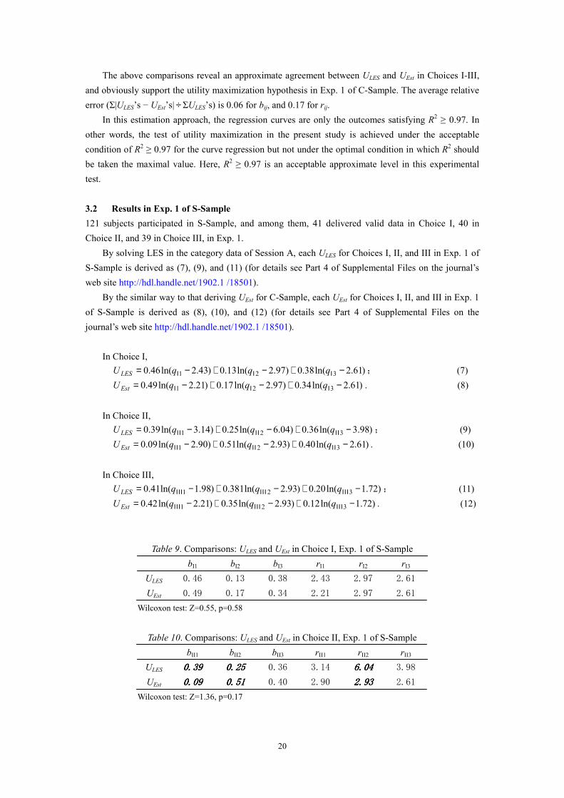
3.2 Results in Exp. 1 of S-Sample

121 subjects participated in S-Sample, and among them, 41 delivered valid data in Choice I, 40 in

Choice II, and 39 in Choice III, in Exp. 1.

By solving LES in the category data of Session A, each ULES for Choices I, II, and III in Exp. 1 of

S-Sample is derived as (7), (9), and (11) (for details see Part 4 of Supplemental Files on the journal’s

web site http://hdl.handle.net/1902.1 /18501).

By the similar way to that deriving UEst for C-Sample, each UEst for Choices I, II, and III in Exp. 1

of S-Sample is derived as (8), (10), and (12) (for details see Part 4 of Supplemental Files on the

journal’s web site http://hdl.handle.net/1902.1 /18501).

In Choice I,

)61.2ln(38.0)97.2ln(13.0)43.2ln(46.0 321 −+−+−= ΙΙΙ qqqU LES ； (7)

)61.2ln(34.0)97.2ln(17.0)21.2ln(49.0 321 −+−+−= ΙΙΙ qqqU Est . (8)

In Choice II,

)98.3ln(36.0)04.6ln(25.0)14.3ln(39.0 321 −+−+−= ΙΙΙΙΙΙ qqqU LES ； (9)


In Choice III,

)72.1ln(20.0)93.2ln(381.0)98.1ln(41.0 321 −+−+−= ΙΙΙΙΙΙΙΙΙ qqqU LES ； (11)


Table 9. Comparisons: ULES and UEst in Choice I, Exp. 1 of S-Sample

bI1 bI2 bI3 rI1 rI2 rI3

ULES 0.46 0.13 0.38 2.43 2.97 2.61

UEst 0.49 0.17 0.34 2.21 2.97 2.61


Table 10. Comparisons: ULES and UEst in Choice II, Exp. 1 of S-Sample


ULES 0.30.30.30.39999 0.20.20.20.25555 0.36 3.14 6.6.6.6.00004444 3.98

UEst 0.090.090.090.09 0.510.510.510.51 0.40 2.90 2.932.932.932.93 2.61


21

Table 11. Comparisons: ULES and UEst in Choice III, Exp. 1 of S-Sample


ULES 0.41 0.38 0.20 1.98 2.93 1.72

UEst 0.42 0.35 0.22 2.21 2.93 1.72


Tables 9-11 collect the comparisons between ULES and UEst for the values of bij and rij contained in

(7)-(12).

Among the eighteen pairwise comparisons shown in Tables 9-11, except of three showing

disagreements (the difference is larger than 40%) in Table 10 (indicated by italic and boldfaced figures),

fifteen comparisons present an approximate agreement between ULES and UEst. About 83% of the

comparisons support the utility maximization hypothesis in Exp. 1 of S-Sample. After omitting the

three disagreeing comparisons in Table 10, the average relative error for the rest fifteen comparisons is

0.09 for bij, and 0.10 for rij.

The comparisons between ULES and UEst in Tables 9 and 11 support the utility maximization in

Choices I and III of Exp. 1 for S-Sample. But in Choice II (Table 10), the disagreeing ones occupy a

half of the comparisons. Choice II in Exp. 1 of S-Sample fails in the test.

3.3 Results in Exp. 2 of S-Sample

Among 121 subjects in S-Sample, 28 delivered valid data in Choices I, II, and III of Exp. 2. However,

the calculation outcome for the estimation of Choice I diverges, and leads to Choice I failing in the test

(see Part 5 of Supplemental Files on the journal’s web site http://hdl.handle.net/1902.1 /18501). Thus,

only Choices II and III in Exp. 2 will be tested below.

By solving LES in the category data of Session A, each ULES for Choices II and III in Exp. 2 of

S-Sample is derived as (13) and (15) (for details please see Part 5 of Supplemental Files).

By the similar way to that deriving UEst for C-Sample, each UEst for Choices I-III in Exp. 2 of

S-Sample is derived as (14) and (16) (for details please see Part 5 of Supplemental Files ).

In Choice II,

)77.0ln(24.0)74.0ln(18.0)59.2ln(58.0 321 −+−+−= ΙΙΙΙΙΙ qqqU LES ; (13)


In Choice III,

)72.1ln(34.0)46.1ln(12.0)91.3ln(52.0 321 −+−+−= ΙΙΙΙΙΙΙΙΙ qqqU LES ; (15)


Tables 12 and 13 collect the comparisons between ULES and UEst for the values of bij and rij

contained in (13)-(16).

Table 12. Comparisons: ULES and UEst in Choice II of Exp. 2


ULES 0.58 0.18 0.24 2.59 0.74 0.77

UEst 0.63 0.13 0.24 2.59 0.90 0.77


22

Table 13. Comparisons: ULES and UEst in Choice III of Exp. 2


ULES 0.52 0.120.120.120.12 0.34 3.91 1.46 1.72

UEst 0.50 0.260.260.260.26 0.24 3.25 0.90 1.72


Except of the comparison of bIII2 indicating a disagreement (the difference is larger than 40%) in

Table 13, overall, they also reveal an approximate agreement between ULES and UEst in Choices II and

III respectively, and thus support the utility maximization hypothesis in Exp. 2 of S-Sample. After

omitting the disagreeing comparison of bIII2 in Table 13, the average relative errors is 0.12 for bij, and

0.14 for rij.

3.4 Summaries for the experimental results

This is an acceptable experimental test with an acceptable approximate level of R2 ≥ 0.97 for the curve

regression, but not an optimal experimental test that requires the maximal value of R2 for the curve

regression.

In eight sets of tests (Tables 6~13), except of a Choice II in Exp. 1 (Table 10), the results reveal the

approximate but systematic agreements between the paired ULES and UEst at the relative error levels

0.06~0.17 for parameter comparisons. The eight sets of tests contain forty-eight pairs of parameter

comparisons in sum, and among them, forty-four pairs deliver agreeing outcomes, occupying a

proportion about 92%, four pairs deliver disagreeing results, occupying a proportion about 8%. Overall,

the experimental results definitively support the utility maximization hypothesis.

As far as the experiments have revealed, the utility maximization holds for both Exp. 1 using

substitutable goods and Exp. 2 using un-substitutable goods. The utility maximization appears

robustness in subjects’ choice behaviors in the two kinds of commodity bundles.

In the above tests, cross affections between different kernels in a choice bundle were naturally

reflected in ULES but, to simplify the experimental procedure, were not taken into account in UEst. UEst

was determined by the measures of utility scales that only relied on the assigned quantities and unit

prices but were irrelevant to the cross affections between different kernels in a choice bundle. For

example, in Choices II and III of Exp. 1 or Exp. 2, rII2 and rIII2 in corresponding UEst are the same

because their assigned prices are the same in Choices II and III (see Tables 2 and 4). It should result

errors in the comparisons between ULES and UEst in these cases. Among four disagreements (see the

italic and boldfaced figures in Tables 10 and 13), three appear in the comparisons of rII2 or bII2, which

are directly or indirectly determined through utility scales delivering the estimated values of rII2 or rIII2.

Therefore, it can be expected that if these cross affections were taken into account, the agreement in the

test would be improved.

In the utility-scale estimate, an easy and feasible treatment for incorporating with the cross

affections between different kernels in a choice bundle is that put the unit price information of other

two kernels in the same choice bundle together with the inquired kernel in an inquiry card, and let the

subject report his bid unit price by comparing with the other two kernels. For example, in Choice II of

Exp. 1, the contents of the inquiry card for “the almond with offered unit price 0.30/bag and assigned

quantity 6” are changed into “the unit price for pistachio is 0.70/bag and for cashew nut is 0.50/bag, if

you are asked to buy 6 bags of almond with offered unit price 0.30/bag, by comparing with the unit

23

prices of pistachio and cashew nut, your bid unit price will be ( )” as shown in Fig. 2.

Almond: 6 bags

Unit price: ¥0.30/bag

Your bid unit price: (¥ )

Please compare

Pistachio: ¥0.70/bag

Cashew nut: ¥0.50/bag

Fig 2. An example for the changed unit price inquiry card. It means “the unit price for pistachio is

0.70/bag and for cashew nut is 0.50/bag. If you are asked to buy 6 bags of almond with offered unit

price 0.30/bag, by comparing with the unit prices of pistachio and cashew nut, your bid unit price will

be ( )”.

The probing experiments offered some evidences implying that the precision of UEst would be

improved greatly in such a treatment. However, the probing experiment also showed that the valid rate

would greatly lower to about 6% if this change were introduced in the inquiry card in Exp. 1. The

experiment may weaken its representativeness as a measure to normal purchase behaviors at so low a

valid rate. The causes of low valid rate may include: 1) in this case, a subject was asked to estimate all

nine utility scales that contain forty-five inquiry cards in sum, but usually the valid rate evidently got to

decrease when the number of inquiry cards is above twenty five; and 2) too many comparisons in a

inquiry card tired the subject.

Another way to improve the test may be that discriminate the preference types by Choice I, and

then, respectively test the subsamples basing on different preference categories. It will greatly enhance

the precise of ULES and UEst but require a very big sample.

As the first experimental test of cardinal utility maximization and a methodological exploration, I

finally chose the simplified program but not the more precise one so that we can concentrate on the

fundamental issues. In fact, the simplified experiments have contributed valuable clues to evaluate the

test of utility maximization. With the mentioned imperfectness of the simplified test, this paper is of

course only an initial probe but, meanwhile, an effective new beginning in the field of utility

maximization test.

4 Concluding remarks

4.1 Major findings

The findings in the experimental test can be interpreted from three aspects.

First, we can test cardinal utility maximization by the experiment, and the experimental results

support the cardinal utility maximization. It is therefore concluded that the cardinal marginal utility

theory has found its empirical foundation in an explicit experimental procedure. It is not only an

inspiring evidence but also a methodological progress for the utility maximization thought. Even

though it is late for more than one-hundred-fifty years, after all, Gossen’s genius has been eventually

combined with and preliminarily supported by the experimental observations.

24

Second, the linear combination of measurable logarithmic laws for economic judgments is a proper

operational definition for Klein-Rubin utility function, furthermore, the utility scaling approach

following psychophysics paradigm (e.g., He, 2012; Galanter, 1962, 1990) offers an appropriate

measure for the cardinal utility theory. The present study further confirms the conclusion presented in

He, 2012: Utility is the subjective quantities of commodities in the utility maximization of LES.

Finally, economics should re-evaluate cardinal utility theory on the basis of behavioral

observations. The cardinal utility maximization is not only measurable but also more measurable than

the ordinal utility maximization, especially, than the revealed preference maximization. In evident, for

multi-commodity choices the cardinal utility maximization can be more clearly, rigorously, and validly

tested in a psychophysics-econometrics paradigm than the ordinal one in a pair-wise comparison way

that may be disturbed by elicitation effects, preference reversals, and etc (e.g., Fredrick and Fischhoff,

1998; Slovic and Lichtenstein, 1983). A new combining point associating positive behavioral studies

with traditional theoretical analyses has emerged, in which classical and contemporary economic

thoughts will together contribute their wisdoms on a common stage of the positive theory.

4.2 Emotion utility and perception utility

Bentham’s utility is described by pleasure, happiness, satisfaction, and so on, referring to a kind of

emotional attribute, can be called “emotion utility”; combining the psychophysical analysis with the

econometric modeling discussion, He, 2012 and the present study reveal that utility is the subjective

quantity of commodity or evaluation, referring to a kind of perceptional attribute, can be called

“perception utility”. The utility research should deal with the two utility concepts but not solely

Bentham’s type.

A corollary derived from econometric models and the present study is that importance of the

quantitative perception exceeds the emotional evaluation in one’s economic choices. Benthamists

perhaps misunderstood an economic choice as an enjoyment choice. In an economic choice, such as

purchase choice, exchange choice, and risk choice, the first determinant is “whether it is worth to pay”,

a comparison between subjective quantities, but not “whether I am pleasant” that is usually seen in an

enjoyment choice, such as eating an apple or a bread, watching a football game or a movie, and

accepting an unfair proposal or rejecting it, in which one seeks a physiological or psychological gain.

The distinction between perception utility and emotion utility comes from and is in turn used to

interpret the difference between economic choice and enjoyment choice. The utility analysis should

base on the discrimination between economic choice and enjoyment choice.

In the electrical-power massage experiment reported in He, 2012, the instruction addressed to

subjects contained the following contents (see page 2 in Supplemental Files for He, 2012 on the

journal’s web site http://hdl.handle.net/1902.1/17166):

Usually there are two types of evaluating massages. One is basing on the degree of your

comfortableness, namely, if you feel more comfortableness in a massage, you will evaluate a

higher price, and if you feel little comfortableness, you will evaluate a very low price, without

referring to the massage duration in time. This is not the evaluating type the experiment wants.

Another evaluating type is basing on the massage duration in time. This is the evaluating type

the experiment wants. You should price a presented massage by concentrating on the massage

duration but not your comfortableness in the experiment. Just like in an electrical-power

massage cure, the price is determined only by the massage duration but not one’s

25

comfortableness. We want to know how you intuitively evaluate price only basing on the

massage consumption quantity.

Such an instruction obviously let subjects judge by the perception utility, and thus, subjects

delivered their utility estimates identified with the forms of sensation scale in psychophysics in the

electrical-power massage experiment (He, 2012). Nevertheless if subjects had been instructed to

evaluate the massage by their comfortableness, i.e., by their emotion utility, subjects would have

reported their utility estimates without any regularity, which was indeed the observed results. In other

words, perception and emotion utilities are two different types of judgments, and the former follows

psychophysical rules but the latter not. We have experimentally verified the perception utility

maximization. Does emotion utility maximization exist? Certainly, it is important to discriminate

emotion and perception utilities.

Benthamists and econometricians had respectively worked in the two different domains long ago.

The perception utility has broadly used in economic empirical and experimental studies to determine

utility functions or value functions in various models, such as the econometric models (e.g. Stone, 1954;

Liuch, 1973) and risk-choice models (e.g., Tversky and Kahneman, 1992; Gonzalez and Wu, 1999).

Whether “emotion” itself means “irrational”, and is there the utility maximization model for the

enjoyment choice? We should perhaps take into account such a possibility that the emotion utility

exists but no maximization can be made for it.

In Galanter (e.g. 1962)’s study, he asked subjects to report a money amount matching to a double

happiness that a gift of $10, $100, or $1,000 would bring them, and derived a power function, a typical

psychophysical law, from his experimental data. That is a perception utility measure converted from

emotion utility by the instruction such as “a double happiness that a gift of $10, $100, or $1,000 would

bring you”. Emotion utility and perception utility seem not completely irrelevant. However, how do we

see the difference between “a double happiness” and a simple “comfortableness”? “A double

happiness” seems not a natural judgment appearing in choice behaviors but a simple “comfortableness”

seems more natural. They have so distinct effects in utility estimates. We perhaps know little about the

properties of emotion utility.

The present study only discussed the Klein-Rubin utility maximization model in depth, are the

utility functions contained in other econometric utility maximization models also construct-able and

measurable in a perception utility framework?

Current ultimatum games used mixed utility judgments, in which unfair feelings (related with

enjoyment choice) mix with some monetary return (related with economic choice). Could we conceive

an ultimatum game mainly involving the emotion utility judgment or perception utility judgment singly

so that we can depart the emotion effect and perception effect in bargaining behaviors? Furthermore,

how do the emotion utility and perception utility affect the difference of responders’ rejection behaviors

between the moderate and very high stake sizes (e.g. Andersen et al., 2011)?

And so on.

We may just begin, and we will need more knowledge to clarify the attributes and functions of the

emotion utility and perception utility.

ReferencesReferencesReferencesReferences

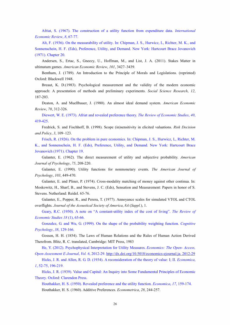
26

Afriat, S. (1967). The construction of a utility function from expenditure data. International

Economic Review, 8, 67-77.

Alt, F. (1936). On the measurability of utility. In: Chipman, J. S., Hurwicz, L, Richter, M. K., and

Sonnenschein, H. F. (Eds), Preference, Utility, and Demand. New York: Hartcourt Brace Jovanovich

(1971). Chapter 20.

Andersen, S., Ertac, S., Gneezy, U., Hoffman, M., and List, J. A. (2011). Stakes Matter in

ultimatum games. American Economic Review, 101, 3427–3439.

Bentham, J. (1789). An Introduction to the Principle of Morals and Legislations. (reprinted)

Oxford: Blackwell 1948.

Breaut, K. D.(1983). Psychological measurement and the validity of the modern economic

approach: A presentation of methods and preliminary experiments. Social Science Research, 12,

187-203.

Deaton, A. and Muellbauer, J. (1980). An almost ideal demand system. American Economic

Review, 70, 312-326.

Diewert, W. E. (1973). Afriat and revealed preference theory. The Review of Economic Studies, 40,

419-425.

Fredrick, S. and Fischhoff, B. (1998). Scope (in)sensitivity in elicited valuations. Risk Decision

and Policy, 3, 109–123.

Frisch, R. (1926). On the problem in pure economics. In: Chipman, J. S., Hurwicz, L, Richter, M.

K., and Sonnenschein, H. F. (Eds), Preference, Utility, and Demand. New York: Hartcourt Brace

Jovanovich (1971). Chapter 19.

Galanter, E. (1962). The direct measurement of utility and subjective probability. American

Journal of Psychology, 75, 208-220.

Galanter, E. (1990). Utility functions for nonmonetary events. The American Journal of

Psychology, 103, 449-470.

Galanter, E. and Pliner, P. (1974). Cross-modality matching of money against other continua. In:

Moskowitz, H., Sharf, B., and Stevens, J. C. (Eds), Sensation and Measurement: Papers in honor of S.

Stevens. Netherland: Reidel. 65-76.

Galanter, E., Popper, R., and Perera, T. (1977). Annoyance scales for simulated VTOL and CTOL

overflights. Journal of the Acoustical Society of America, 8A (Suppl.), 1.

Geary, R.C. (1950). A note on “A constant-utility index of the cost of living”. The Review of

Economic Studies 18 (1), 65-66.

Gonzalez, G. and Wu, G. (1999). On the shape of the probability weighting function. Cognitive

Psychology, 38, 129-166.

Gossen, H. H. (1854). The Laws of Human Relations and the Rules of Human Action Derived

Therefrom. Blitz, R. C. translated, Cambridge: MIT Press, 1983

He, Y. (2012). Psychophysical Interpretation for Utility Measures. Economics: The Open- Access,

Open-Assessment E-Journal, Vol. 6, 2012-29. http://dx.doi.org/10.5018/economics-ejournal.ja. 2012-29

Hicks, J. R. and Allen, R. G. D. (1934). A reconsideration of the theory of value: I; II. Economica,

1, 52-75, 196-219.

Hicks, J. R. (1939). Value and Capital: An Inquiry into Some Fundamental Principles of Economic

Theory. Oxford: Clarendon Press.

Houthakker, H. S. (1950). Revealed preference and the utility function. Economica, 17, 159-174.

Houthakker, H. S. (1960). Additive Preferences. Econometrica, 28, 244-257.

27

Intriligator, M. D. (1980). Econometric Models, Techniques, and Applications. New Delhi:

Prentice-Hall. 226–230.

Johnson, W. E. (1913). The pure theory of utility curves. Economic Journal, 23, 483-513.

Kahneman, D., Wakkar, P. P., and Sarin, R. (1997). Back to Bentham? Explorations of experienced

utility. The Quarterly Journal of Economics, (May), 275-405.

Klein, L. R. and Rubin, H. (1947). A Constant-Utility Index of Cost of Living. The Review of

Economic Studies 15 (2), 84-87.

Liuch, C. (1973). The expended linear expenditure system. European Economic Review, 4, 21-32.

MacCrimmon, K. R. and Toda, M. (1969). The experimental determination of indifference curves.

Review of Economic Studies 36, 433–451.

Pareto, V. (1906). Mamuale di Economia Politica. Milano: Società Editrice Libraria.

Parker, S. and Schneider, B. (1988). Conjoint scaling of the utility of money using paired

comparisons. Social Science Research, 17, 277-286.

Samuelson, P. A. (1938). The numerical representation of ordered classifications and the concept

of utility. Review of Economic Studies, 6, 65-70.

Slovic, P. and Lichtenstein, S. (1983). Preference reversals: A broader perspective. American

Economic Review, 73, 596–605.

Stigler, G. J., (1950). The development of utility theory, I. The Journal of Political Economy, 58

(4), 307-327; 58 (5), 373-396.

Stone, R. (1954). Linear expenditure system and demand analysis: An application to the pattern of

British demand. Economics Journal, 64, 511-527.

Theil, H. (1965). The information approach to demand analysis. Econometrica, 33, 67-87.

Thurstone, L. L. (1931). The indifference function. Journal of Social Psychology, 2, 139–167.

Tversky, A. and Kahneman, D. (1992). Advances in prospect theory: Cumulative representation of

uncertainty. Journal of Risk and Uncertainty, 5, 297-324.

Varian, H. R. (1982). The nonparametric approach to demand analysis. Econometrica, 50, 99-110.

Varian, H. R. (1983). Non-parametric tests of consumer behavior. The Review of Economic Studies,

50, 99-100.

Varian, H. R. (2009). Intermediate Microeconomics: A Modern Approach. (Eighth Ed.). New York:

W. W. Norton & Company. Chapter 7.

To invited reader

Documents

Transcript of To invited reader