To Do List Reading for next time: Peter Chen and David Patterson, A New Approach to I/O Performance...
52
To Do List Reading for next time: Peter Chen and David Patterson, A New Approach to I/O Performance Evaluation – Self-Scaling I/O Benchmarks, Predicted I/O Performance, SIGMETRICS 1993. Assignment for Feb 9 (week from this coming Thursday): Project pre-proposal.
-
Upload
randolph-griffith -
Category
Documents
-
view
212 -
download
0
Transcript of To Do List Reading for next time: Peter Chen and David Patterson, A New Approach to I/O Performance...

To Do List
Reading for next time: Peter Chen and David Patterson,A New Approach to I/O Performance Evaluation – Self-Scaling I/O Benchmarks, Predicted I/O Performance, SIGMETRICS 1993.
Assignment for Feb 9 (week from this coming Thursday): Project pre-proposal.

Workloads Experimentalenvironment
prototypereal sys
exec-driven
sim
trace-driven
sim
stochasticsim
Liveworkload
Benchmarkapplications
Micro-benchmarkprograms
Syntheticbenchmarkprograms
TracesDistributions
& otherstatistics
monitor
analysis
generator Synthetictraces“Real”
workloads
Made-up
© 2003, Carla Ellis
Datasets
Found insample of Mobisys papers

Workloads Discussion
Mobisys submissions
• Ad hoc routing:
– Synthetic workload with source nodes generating packets at given rate (1 packet per second) and nodes move according to “waypoint” model.
• Full system profiling
– Mediabench
• Device driver replacement
– www.textuality.com/bonnie – Unix file system benchmark (reads, writes, lseeks)
– www.netperf.org - networking (TCP, IP, UDP, Unix sockets)
© 2003, Carla Ellis

• 2 Hoarding (caching/prefetching) papers:– Home-grown web user request logs– File system traces used for Coda and Seer projects previously
(open, close)• Web transcoding for mobile devices
– User study with canned exercises• Bluetooth and WiFi
– Benchmark programs: idle, 2 file transfers, www, videos• Sensor network for weather monitoring in forest fire zones
– Deployed with live workload (real weather)• Wireless web browsing
– Synthetic workload based on “User Centric Walk”• Energy reduction
– Microbenchmarks to exercise individual components of platform and measure the power used during their execution (known “engineered” behavior)

Workloads Experimentalenvironment
prototypereal sys
exec-driven
sim
trace-driven
sim
stochasticsim
Liveworkload
Benchmarkapplications
Micro-benchmarkprograms
Syntheticbenchmarkprograms
TracesDistributions
& otherstatistics
monitor
analysis
generator Synthetictraces“Real”
workloads
Made-up
© 2003, Carla Ellis
Datasets
You are here

© 1998, Geoff Kuenning
System ProvidedMetrics and Utilities
• Many operating systems provide users access to some metrics
• Most operating systems also keep some form of accounting logs
• Lots of information can be gathered this way

© 1998, Geoff Kuenning
What a Typical System Provides
• Timing tools• Process state tools• System state tools• OS accounting logs• Logs for important systems programs
© 1998, Geoff Kuenning
Time
• Many OSs provide system calls that start and stop timers– Allows you to time how long things took
• Usually, only elapsed time measurable– Not necessarily time spent running
particular process• So care is required to capture real meaning of
timings

© 1998, Geoff Kuenning
Timing Tools
• Tools that time the execution of a process• Often several different times are provided• E.g., Unix time command provides system
time, user time, and elapsed time• Various components of the times provided
may depend on other system activities– So just calling time on a command may
not tell the whole story

Timer Overhead
start = time();
execute_event ();
end = time();
elapsed_time = (end – start) * t_cycle;
calltime
readclock
Eventbegins
Eventends;call time
readclock
te
tm
Rule of thumb:te should be 100xlarger than overhead

Uses of Time
• Measurements – durations of activities– Stability – ability to maintain constant frequency
• Environmental factors (temperature) or age• Synchronization protocols that adjust clock
• Coordinating events– Synchronized clocks
• Scheduling dynamic events at a particular time in the future or periodically.– Frequency– Accuracy– Relative or absolute time?

Time Definitions• Clock stability – how well it maintains a
constant frequency– Short term – temperature– Long term – aging of oscillator
• Clock accuracy – how well its frequency and time compare with standard

Time Definitions
• Offset – time difference between 2 clocks300s at 100 sSynchronize
• Skew – frequency difference between 2 clocksSlope 3s/s

© 1998, Geoff Kuenning
Process State Tools
• Many systems have ways for users to find out about the state of their processes
• Typically provide information about– Time spent running process so far– Size of process– Status of process– Priority of process– I/O history of process

© 1998, Geoff Kuenning
Using Process State Tools
• Typically, you can’t monitor process state continuously– Updates not provided every time things
change• You get snapshots on demand
– So most useful for sampling monitors

© 1998, Geoff Kuenning
System State Tools
• Many systems allow some users to examine their internal state– E.g., virtual memory statistics– Or length of various queues
• Often available only to privileged users• Typically, understanding them requires
substantial expertise – And they are only useful for specific
purposes

© 1998, Geoff Kuenning
Logs
• Can log arbitrarily complex data about an event
• But more complex data takes more space• Typically, log data into a reserved buffer• When full, request for buffer to be written to
disk– Often want a second buffer to gather data
while awaiting disk write

© 1998, Geoff Kuenning
Designing a Log Entry
• What form should a log entry take?• Designing for compactness vs. human
readability– Former better for most purposes– Latter useful for system debugging– But make sure no important information is
lost in compacting the log entry

© 1998, Geoff Kuenning
OS Accounting Logs
• Many operating systems maintain logs of significant events– Based either on event-driven or sampling
monitors• Examples:
– logins– full file systems– device failures

© 1998, Geoff Kuenning
System SoftwareAccounting Logs
• Often, non-OS systems programs keep logs• E.g., mail programs, web servers• Usually only useful for monitoring those
programs• But sometimes can provide indirect
information– E.g., a notice of a failure to open a
connection to a name server may indicate machine failure

Workloads Experimentalenvironment
prototypereal sys
exec-driven
sim
trace-driven
sim
stochasticsim
Liveworkload
Benchmarkapplications
Micro-benchmarkprograms
Syntheticbenchmarkprograms
TracesDistributions
& otherstatistics
monitor
analysis
generator Synthetictraces“Real”
workloads
Made-up
© 2003, Carla Ellis
Datasets
You are here
© 1998, Geoff Kuenning
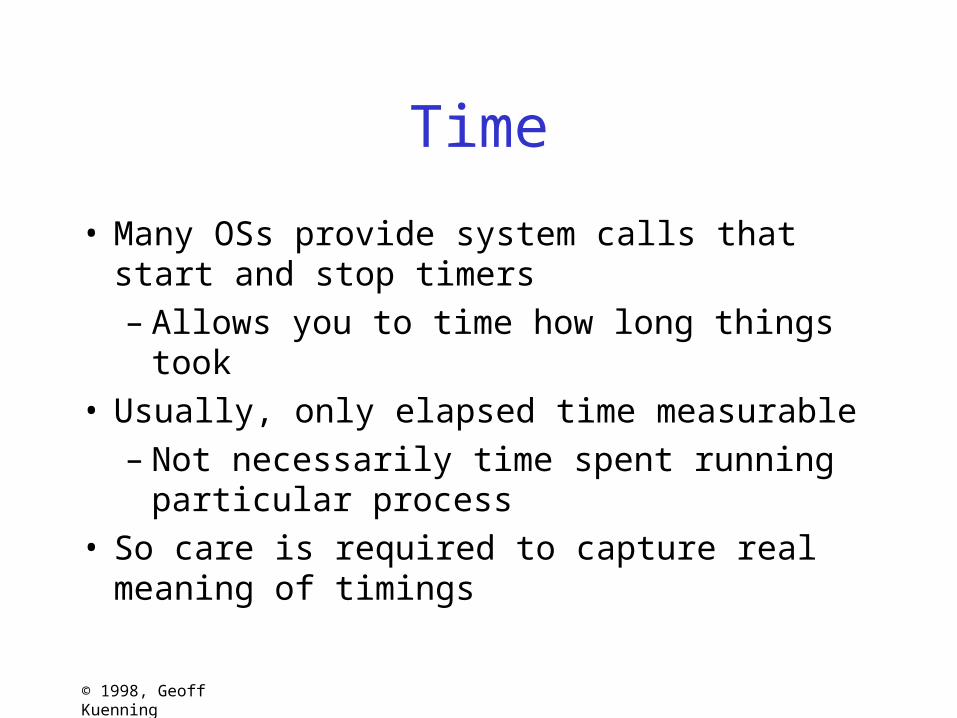
Workload Characterization
• Jain’s topics in Chapter 6– Terminology– Techniques
• Averaging• Specifying Dispersion• Single-Parameter Histograms• Multi-Parameter Histograms• Principal-Component Analysis• Markov Models• Clustering

© 1998, Geoff Kuenning
Workload Characterization
Terminology• User (maybe nonhuman) requests service
– Also called workload component or workload unit
• Workload parameters or workload features model or characterize the workload

© 1998, Geoff Kuenning
Selecting Workload Components
• Most important is that components be external: at the interface of the SUT
• Components should be homogeneous
• Should characterize activities of interest to the study
Web Client
Network
TCP/IP Connections
Web Server
HTTP Requests
File System
Web Page File Accesses
Disk Drive
Disk Transfers
Web Page Visits

© 1998, Geoff Kuenning
ChoosingWorkload Parameters
• Select parameters that depend only on workload (not on SUT)
• Prefer controllable parameters• Omit parameters that have no effect on
system, even if important in real world

An Analysis of Internet Content Delivery Systems Stefan Saroiu, Krishna Gummadi, Richard Dunn, Steve Gribble, Hank
LevyOSDI 2004
Object Size CDF
0%
20%
40%
60%
80%
100%
0 1 10 100 1,000 10,000 100,000 1,000,000Object Size (KB)
% O
bje
cts
Kazaa
AkamaiWWW
Gnutella

© 1998, Geoff Kuenning
Averaging
Basic character of a parameter is its average value
• Mean• Median• Mode• All specify center of location of the distribution
of the observations in the sample

© 1998, Geoff Kuenning
Sample Mean (Arithmetic)
• Take sum of all observations• Divide by the number of observations• Assumes all of the observed values are
equally likely to occur.• More affected by outliers than median or
mode• Mean is a linear property
– Mean of sum is sum of means– Not true for median and mode

© 1998, Geoff Kuenning
Sample Median
• Sort the observations– In increasing order
• Take the observation in the middle of the series– If even # of data points, take mean of 2
middle ones• More resistant to outliers
– But not all points given “equal weight”

© 1998, Geoff Kuenning
Sample Mode
• Plot a histogram of the observations– Using existing categories– Or dividing ranges into buckets
• Choose the midpoint of the bucket where the histogram peaks– For categorical variables, the most
frequently occurring• Effectively ignores much of the sample

© 1998, Geoff Kuenning
Characteristics of Mean, Median, and Mode
• Mean and median always exist and are unique
• Mode may or may not exist– If there is a mode, there may be more than
one• Mean, median and mode may be identical
– Or may all be different– Or some of them may be the same

© 1998, Geoff Kuenning
Mean, Median, and Mode Identical
MedianMeanMode
x
pdff(x)

© 1998, Geoff Kuenning
Median, Mean, and ModeAll Different
Mean
MedianMode
pdff(x)
x

© 1998, Geoff Kuenning
So, Which Should I Use?
• Depends on characteristics of the metric• If data is categorical, use mode• If a total of all observations makes sense, use
arithmetic mean– Inappropriate for rates
• If the distribution is skewed, use median• Otherwise, consider other definitions of mean
(e.g. harmonic)• But think about what you’re choosing

© 1998, Geoff Kuenning
Some Examples
• Most-used resource in system– Mode
• Interarrival times– Mean
• Load– Median

© 1998, Geoff Kuenning
Specifying Dispersion
• Most parameters are non-uniform• Usually, you need to know how much the rest
of the data set varies from that index of central tendency
• Specifying variance or standard deviation brings a major improvement over average
• Average and s.d. (or C.O.V.) together allow workloads to be grouped into classes– Still ignores exact distribution

© 1998, Geoff Kuenning
Why Is Variability Important?
• Consider two Web servers:– Server A services all requests in 1 second– Server B
• Services 90% of all requests in .5 seconds• But 10% in 55 seconds
– Both have mean service times of 1 second– But which would you prefer to use?

© 1998, Geoff Kuenning
Range
• Minimum and maximum values in data set• Can be kept track of as data values arrive• Variability characterized by difference
between minimum and maximum• Often not useful, due to outliers• Minimum tends to go to zero• Maximum tends to increase over time• Not useful for unbounded variables

© 1998, Geoff Kuenning
Example of Range
• For data set
2, 5.4, -17, 2056, 445, -4.8, 84.3, 92, 27, -10– Maximum is 2056– Minimum is -17– Range is 2073– While arithmetic mean is 268

© 1998, Geoff Kuenning
Variance (and Its Cousins)
• Sample variance is
• Variance is expressed in units of the measured quantity squared– Which isn’t always easy to understand
• Standard deviation and the coefficient of variation are derived from variance
sn
x xii
n2 2
1
1
1

© 1998, Geoff Kuenning
Variance Example
• For data set
2, 5.4, -17, 2056, 445, -4.8, 84.3, 92, 27, -10• Variance is 413746.6• You can see the problem with variance:
– Given a mean of 268, what does that variance indicate?

© 1998, Geoff Kuenning
Standard Deviation
• The square root of the variance• In the same units as the units of the metric• So easier to compare to the metric

© 1998, Geoff Kuenning
Standard Deviation Example
• For the sample set we’ve been using, standard deviation is 643
• Given a mean of 268, clearly the standard deviation shows a lot of variability from the mean

© 1998, Geoff Kuenning
Coefficient of Variation
• The ratio of the mean and standard deviation• Normalizes the units of these quantities into a
ratio or percentage• Often abbreviated C.O.V.

© 1998, Geoff Kuenning
Coefficient of Variation Example
• For the sample set we’ve been using, standard deviation is 643
• The mean of 268• So the C.O.V. is 643/268
= 2.4

© 1998, Geoff Kuenning
Percentiles
• Specification of how observations fall into buckets– e.g., the 5-percentile is the observation that
is at the lower 5% of the set– While the 95-percentile is the observation
at the 95% boundary of the set• Useful even for unbounded variables

© 1998, Geoff Kuenning
Relatives of Percentiles
• Quantiles - fraction between 0 and 1– Instead of percentage– Also called fractiles
• Deciles - percentiles at the 10% boundaries– First is 10-percentile, second is 20-percentile, etc.
• Quartiles - divide data set into four parts– 25% of sample below first quartile, etc.– Second quartile is also the median

© 1998, Geoff Kuenning
Single-Parameter Histograms
• Fit probability distribution to shape of histogram
• Ignores multiple-parameter correlations

© 1998, Geoff Kuenning
Plotting a Histogram
Suitable if you have a relatively large number of data points
1. Determine range of observations
2. Divide range into buckets
3. Count number of observations in each bucket
4. Divide by total number of observations and plot it as column chart
© 1998, Geoff Kuenning
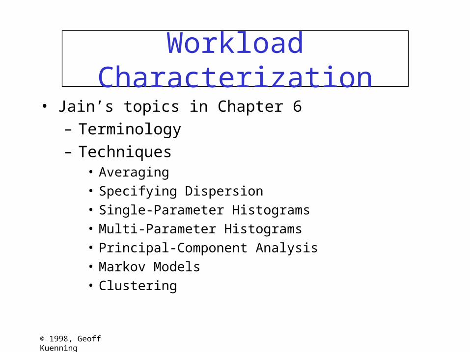
Problem WithHistogram Approach
• Determining cell size– If too small, too few observations per cell– If too large, no useful details in plot
• If fewer than five observations in a cell, cell size is too small

© 1998, Geoff Kuenning
Multi-Parameter Histograms
• Use 3-D plotting package to show 2 parameters– Or plot each datum as 2-D point and look
for “black spots”• Shows correlations
– Allows identification of important parameters
• Not practical for 3 or more parameters

© 1998, Geoff Kuenning
Zipf Distribution
• A few very frequently occurring elements• A huge number of very rarely occurring elements• Data show web page access follows this pattern –
popularity distribution
log rank
log freq
rank
freq