
TO APPEAR ON IEEE TRANSACTIONS ON POWER...
8
TO APPEAR ON IEEE TRANSACTIONS ON POWER DELIVERY 1 An Experimental Characterization of the PLC Noise at the Source Massimo Antoniali, Fabio Versolatto, Member, IEEE, and Andrea M. Tonello Senior Member, IEEE Abstract—Power line communications (PLC) are affected by severe noise. In the in-home scenario, the household appliances are the main sources of noise, when they are fed and running, as they inject noise in the frequencies where PLC operate. This work presents a methodology for the characterization of the noise generated by devices connected to the power grid. The methodology is applied to study a number of household appliances. The study enables to a) identify the most noisy devices from which PLC transceivers should be kept far away, b) characterize the noise both in the time and the frequency domain, c) address the definition of noise limits from an EMC regulator perspective, and d) quantify the amplitude of the impulsive noise that may damage the analog front-end of the PLC transceiver. The work addresses both the noise during the normal op- erating conditions of the household appliances, and the noise generated during transients, i.e., when the device is connected, disconnected, switched on or off. In this respect, it is shown that transients may lead to noise spikes that exceed tens of Volts. Index Terms—power line communications, impulsive noise, time-frequency analysis I. I NTRODUCTION The communication technologies that allow exploiting the power delivery network to convey data content are commonly referred to as power line communications (PLC). The power delivery network was not designed for communication pur- poses and thus PLC encounter several criticalities, as for instance, severe noise impairments [1]. From a PLC perspective, one of the most disruptive noise components is the differential-mode noise. In single phase networks, the differential-mode noise currents flow on the phase and neutral wires with the same intensity but opposite direction. Common-mode noise can also be present and it is generated by currents that flow with the same direction on both wires. Herein, we focus on the differential-mode noise. The characterization of the PLC noise requires an extensive experimental activity that can be carried out either at the port where the receiver modem is connected or at the ports where the main sources of noise are connected. The former approach provides information about the overall noise that impairs the communication. The latter approach allows the characterization of the main sources of noise through the evaluation of the level of disturbance that they individually inject in a certain point of the grid. A comprehensive characterization of the PLC noise at the receiver port was provided in [2]. It was shown that the PLC Manuscript submitted on September 15, 2014, revised on January 9, 2015 and on March 24, 2015, accepted on June 14, 2015. The work herein presented has been carried out in part at the University of Udine, Italy. The work of A. Tonello has been carried out at the University of Klagenfurt, Austria (e-mail: {massimo.antoniali, fabio.versolatto}@uniud.it, [email protected]). noise consists of background and impulsive noise components. The background noise is a combination of conducted and coupled noise contributions. The conducted noise contributions are amenable mostly to the devices connected to the power delivery network. The coupled noise contributions are due to the radio signals that are captured by the wirings. Typically, the background noise is modelled as stationary additive colored noise with a frequency decreasing power spectral density (PSD) profile. According to measures, the PSD decay profile can be modeled as a power function [3], or as an exponential function [4] of the frequency. Furthermore, the distribution of the amplitude in the time-domain can be fitted by the Middleton’s class A [5] or the Nakagami-m distribution [6]. Some further studies reveal that the normal assumption on the noise statistics holds true if the periodic time-variant nature of the noise is accounted [7], and the impulsive noise contributions are removed from the noise measure [8]. The impulsive noise is unstationary and it can be a) cy- clostationary with a repetition rate that is equal to or double that of the mains period, b) bursty and cyclostationary with a burst repetition rate that is high, between 50 and 200 kHz, or c) aperiodic. In the literature, the first two components are referred to as impulsive noise periodic synchronous and asynchronous with the mains frequency [9]. They exhibit a repetition rate equal or greater than the mains period. In particular, the periodic synchronous noise is originated by the silicon controlled rectifiers (SCR), while the asynchronous noise is due to, for instance, the switching activity of the power supplies. A time-frequency procedure to extract the periodic noise terms from the measures is presented in [8]. A model of the periodic noise terms that is based on a deseasonalized autoregressive moving average is discussed in [10]. The aperiodic noise is the most unpredictable component and it is due to the connection and disconnection of the appliances from the power delivery network. The amplitude of the aperiodic noise can be significantly larger than that of the other impulsive noise components. Beside the amplitude, the aperiodic impulsive noise is described by the duration and the inter-arrival time [11]. The statistics of these quantities depends on how the impulsive noise events are identified and measured. Several works addressed the characterization of the aperiodic impulsive noise. Among these, [9] proposes the use of a Markov-chain model to describe the same quantities in a combined fashion. Most of the papers above are focused on the frequency range up to 30 MHz. The study of the PLC noise at the source is important for PLC technology manufacturers because it provides a clear indication about the devices that inject large noise components and that should be kept far from the PLC equipment. In a dual This is the author's version of an article that has been published in this journal. Changes were made to this version by the publisher prior to publication. The final version of record is available at http://dx.doi.org/10.1109/TPWRD.2015.2452939 Copyright (c) 2016 IEEE. Personal use is permitted. For any other purposes, permission must be obtained from the IEEE by emailing [email protected].
-
Upload
nguyendien -
Category
Documents
-
view
216 -
download
1
Transcript of TO APPEAR ON IEEE TRANSACTIONS ON POWER...
TO APPEAR ON IEEE TRANSACTIONS ON POWER DELIVERY 1
An Experimental Characterization
of the PLC Noise at the SourceMassimo Antoniali, Fabio Versolatto, Member, IEEE, and Andrea M. Tonello Senior Member, IEEE
Abstract—Power line communications (PLC) are affected bysevere noise. In the in-home scenario, the household appliancesare the main sources of noise, when they are fed and running,as they inject noise in the frequencies where PLC operate.
This work presents a methodology for the characterizationof the noise generated by devices connected to the power grid.The methodology is applied to study a number of householdappliances. The study enables to a) identify the most noisydevices from which PLC transceivers should be kept far away, b)characterize the noise both in the time and the frequency domain,c) address the definition of noise limits from an EMC regulatorperspective, and d) quantify the amplitude of the impulsive noisethat may damage the analog front-end of the PLC transceiver.
The work addresses both the noise during the normal op-erating conditions of the household appliances, and the noisegenerated during transients, i.e., when the device is connected,disconnected, switched on or off. In this respect, it is shown thattransients may lead to noise spikes that exceed tens of Volts.
Index Terms—power line communications, impulsive noise,time-frequency analysis
I. INTRODUCTION
The communication technologies that allow exploiting the
power delivery network to convey data content are commonly
referred to as power line communications (PLC). The power
delivery network was not designed for communication pur-
poses and thus PLC encounter several criticalities, as for
instance, severe noise impairments [1].
From a PLC perspective, one of the most disruptive noise
components is the differential-mode noise. In single phase
networks, the differential-mode noise currents flow on the
phase and neutral wires with the same intensity but opposite
direction. Common-mode noise can also be present and it is
generated by currents that flow with the same direction on
both wires. Herein, we focus on the differential-mode noise.
The characterization of the PLC noise requires an extensive
experimental activity that can be carried out either at the
port where the receiver modem is connected or at the ports
where the main sources of noise are connected. The former
approach provides information about the overall noise that
impairs the communication. The latter approach allows the
characterization of the main sources of noise through the
evaluation of the level of disturbance that they individually
inject in a certain point of the grid.
A comprehensive characterization of the PLC noise at the
receiver port was provided in [2]. It was shown that the PLC
Manuscript submitted on September 15, 2014, revised on January 9, 2015and on March 24, 2015, accepted on June 14, 2015.The work herein presented has been carried out in part at the University ofUdine, Italy. The work of A. Tonello has been carried out at the University ofKlagenfurt, Austria (e-mail: massimo.antoniali, [email protected],[email protected]).
noise consists of background and impulsive noise components.
The background noise is a combination of conducted and
coupled noise contributions. The conducted noise contributions
are amenable mostly to the devices connected to the power
delivery network. The coupled noise contributions are due to
the radio signals that are captured by the wirings. Typically, the
background noise is modelled as stationary additive colored
noise with a frequency decreasing power spectral density
(PSD) profile. According to measures, the PSD decay profile
can be modeled as a power function [3], or as an exponential
function [4] of the frequency. Furthermore, the distribution
of the amplitude in the time-domain can be fitted by the
Middleton’s class A [5] or the Nakagami-m distribution [6].
Some further studies reveal that the normal assumption on
the noise statistics holds true if the periodic time-variant
nature of the noise is accounted [7], and the impulsive noise
contributions are removed from the noise measure [8].
The impulsive noise is unstationary and it can be a) cy-
clostationary with a repetition rate that is equal to or double
that of the mains period, b) bursty and cyclostationary with a
burst repetition rate that is high, between 50 and 200 kHz,
or c) aperiodic. In the literature, the first two components
are referred to as impulsive noise periodic synchronous and
asynchronous with the mains frequency [9]. They exhibit a
repetition rate equal or greater than the mains period. In
particular, the periodic synchronous noise is originated by
the silicon controlled rectifiers (SCR), while the asynchronous
noise is due to, for instance, the switching activity of the power
supplies. A time-frequency procedure to extract the periodic
noise terms from the measures is presented in [8]. A model
of the periodic noise terms that is based on a deseasonalized
autoregressive moving average is discussed in [10].
The aperiodic noise is the most unpredictable component
and it is due to the connection and disconnection of the
appliances from the power delivery network. The amplitude
of the aperiodic noise can be significantly larger than that of
the other impulsive noise components. Beside the amplitude,
the aperiodic impulsive noise is described by the duration and
the inter-arrival time [11]. The statistics of these quantities
depends on how the impulsive noise events are identified and
measured. Several works addressed the characterization of the
aperiodic impulsive noise. Among these, [9] proposes the use
of a Markov-chain model to describe the same quantities in a
combined fashion. Most of the papers above are focused on
the frequency range up to 30 MHz.
The study of the PLC noise at the source is important for
PLC technology manufacturers because it provides a clear
indication about the devices that inject large noise components
and that should be kept far from the PLC equipment. In a dual
This is the author's version of an article that has been published in this journal. Changes were made to this version by the publisher prior to publication.The final version of record is available at http://dx.doi.org/10.1109/TPWRD.2015.2452939
Copyright (c) 2016 IEEE. Personal use is permitted. For any other purposes, permission must be obtained from the IEEE by emailing [email protected].
TO APPEAR ON IEEE TRANSACTIONS ON POWER DELIVERY 2
Device
under test Bro
adb
an
d
Cou
ple
r
Digital storage
oscilloscopeLow pass filter
Power delivery network trigger
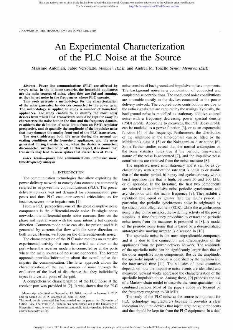
Fig. 1. Schematic representation of the measurement setup.
manner, the study of the PLC noise at the source is important
for EMC regulation bodies as it provides guidelines for the
definition of electromagnetic emission limits to enable the use
of, and the coexistence with, PLC. Furthermore, the study of
the noise at the source provides information on the maximum
amplitude of the high-spikes of the aperiodic impulsive noise.
This is fundamental for the design of the protection circuitry of
the PLC equipment. Finally, we note that, from the measures
of the noise at the source, we can obtain the noise at the
receiver port by taking into account the effect of the channel
response. This can be done by measuring the channel response
or using a channel model. For instance, in [12] the noise at
the source is modeled as in [3] and the channel response is
obtained from a top-down modeling approach. Similarly, in
[13] a top-down channel generator is used while the noise at
the source is measured.
Some results about the noise at the source are presented
in [14]-[15], although limited to the asynchronous impulsive
noise. In particular, [14] shows noise spikes of up to thousands
of Volts by switching on/off the devices, and [15] reveals noise
spikes in the order of tens of Volts for the same events.
The goal of this work is to provide deeper insight on the
noise at the source providing a statistical analysis of the
results of an experimental measurement campaign that we
carried out at the source, on real-life household appliances.
Twelve representative household appliances were selected and
the measurements were performed in the time domain. The
database is well representative and it can be further extended
with new measurement campaigns that share the measurement
procedure and processing herein detailed. The processing
enables separating the noise components and providing a
characterization of each.
Compared to prior works in the literature, in this study,
a) the frequency range is extended up to 100 MHz, b)
an overview of all the noise components generated by the
targeted devices is provided, and c) a novel characterization
of the impulsive noise in power terms to account for both the
amplitude and the duration of the noise spikes is presented.
The analysis allows to identify the intervals of the mains
period during which the noise is higher, and the frequency
intervals that experience the largest noise peaks. The peaks
are amenable to either asynchronous noise components, that
generate equally spaced peaks in the frequency [8], or other
narrow band noise terms, as deterministic sinusoidal tones.
The remainder of the paper is organized as follows. Section
II presents the rationale of the work, the scope, and puts the
emphasis on the usefulness of the results. Section III describes
the measurement configuration that we adopted. Sections IV
and V deal with the noise observed during normal-mode
operating conditions and during transient events, respectively.
Finally, some conclusions follow.
II. RATIONALE
The study of the noise at the source is of great interest for
PLC modem designers and EMC regulators. From a designer
perspective, the noise at the source represents the worst-
case noise scenario as it resembles an installation where the
noise source is close to the transceiver, and its time/frequency
domain analysis is useful to highlight the frequency bands
and the time intervals during which the PLC transmission
should be avoided or made more robust to cope with the
noise impairments. Furthermore, the analysis of the impulsive
noise amplitude and power is beneficial for the design of the
protection circuitry of the analog front end.
From a regulatory perspective, the study of the noise at
the source is important to understand the current emission of
household appliances and their impact on PLC, and to draft
new regulations that would limit further the noise emission
in favor of PLC. For instance, not only during the normal-
mode operating conditions, but also during transient events,
as during switching on/off or plugging in/out a device.
III. MEASUREMENT SETUP AND DEVICE DESCRIPTION
Fig. 1 shows the schematic representation of the time-
domain measurement setup that we adopted. Basically, the
digital storage oscilloscope (DSO) is connected close to the
device under test (DUT). A broadband coupler protects the
equipment from the mains, and a low pass filter (LPF) iso-
lates the DUT from the rest of the power delivery network.
The circuit design of the LPF resembles the electromagnetic
compatibility filter of common appliances and it exhibits an
attenuation in excess of 20 dB in the frequency range below 15
MHz, where the noise components coming from the network
are mostly concentrated.
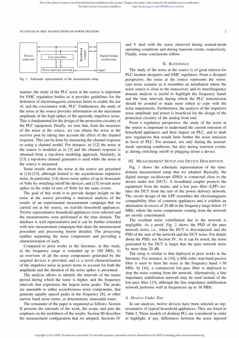
The resultant noise contribution due to the network is
negligible. As a proof, Fig. 2 shows the PSD of the pure
network noise, i.e., when the DUT is disconnected, and the
PSD of the sum of the network and the DUT noise. For details
about the PSD, see Section IV. As it can be noted, the noise
generated by the DUT is larger that the pure network noise
by more than 20 dB.
The setup is similar to that deployed in prior works in the
literature. For instance, in [10], a fifth order stop-band passive
filter is used to limit the noise in the frequency band 1-30
MHz. In [16], a commercial low-pass filter is deployed to
stop the noise coming from the network. Alternatively, a line
impedance stabilization network may be used instead of the
low-pass filter [15], although the line impedance stabilization
network performs well at frequencies up to 30 MHz.
A. Devices Under Test
In our analysis, twelve devices have been selected as rep-
resentative of typical household appliances. They are listed in
Table I. Three models of desktop PCs are considered in order
to highlight, if any, differences between the noise injected
This is the author's version of an article that has been published in this journal. Changes were made to this version by the publisher prior to publication.The final version of record is available at http://dx.doi.org/10.1109/TPWRD.2015.2452939
Copyright (c) 2016 IEEE. Personal use is permitted. For any other purposes, permission must be obtained from the IEEE by emailing [email protected].
TO APPEAR ON IEEE TRANSACTIONS ON POWER DELIVERY 3
0 20 40 60 80 100−170
−160
−150
−140
−130
−120
−110
Frequency (MHz)
Pow
er S
pect
ral D
ensi
ty (
dBV
/Hz)
DUT plus Network Noise PSD
Pure Network Noise PSD
Fig. 2. Power spectral density of the pure network noise and of the purenetwork noise plus the DUT noise.
by their power supplies. The three PCs are distinguished by
the letter A, B, or C and they are from different vendors.
Furthermore, this study targets the noise injected by a light
dimmer when it is set to supply half or a quarter of the
maximum power. The results will show that the light dimmer
injects large periodic noise components during short time
periods of about 1 ms, whose position within the mains period
is a function of the supplied power.
Beside the injected noise, a device is characterized by its
impedance. The impedance of the device is important because
it impacts on the PLC channel characteristics. As the noise,
the device impedance can be time variant. Further, it depends
on the state of the device. For instance, the vacuum cleaner
exhibits an inductive or capacitive behavior when it is switched
on or off, respectively [17]. The study of the device impedance
is beyond the scope of this work and it is detailed in [17], [18].
IV. NORMAL-MODE OPERATING CONDITION
We now consider the noise injected by the household
appliances during their normal operating conditions, i.e., when
they are switched on and running. In particular, let us ana-
lyze the time-variant PSD. Measurements were performed as
follows. The DSO was triggered to the mains cycle and it
was configured to acquire an observation window equal to the
mains period, i.e., 20 ms. The sampling period results from
the ratio between the length of the observation window, i.e.,
T0 = 20 ms, and the memory depth of the DSO which is equal
to 107, yielding T = 2 ns. Hence, the sampling frequency
is 500 MS/s. Such a high value was motivated, initially, by
the purpose of exploring the noise in the maximum frequency
band allowed by the instrument capabilities. As described in
the following, results suggest that the noise is limited to the
lower frequency band, below 20 MHz so that lower sampling
frequencies can be used.
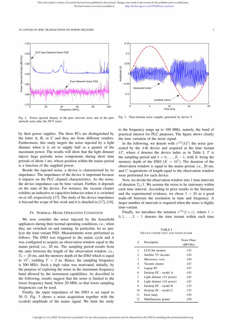
Finally, the input impedance of the DSO is set equal to
50 Ω. Fig. 3 shows a noise acquisition together with the
(scaled) amplitude of the mains signal. We limit the study
0 5 10 15 20
−0.1
−0.05
0
0.05
0.1
0.15
Time (ms)
Am
plitu
de (
V)
(scaled) mains
measured noise
Fig. 3. Time-domain noise samples generated by device 9.
to the frequency range up to 100 MHz, namely, the band of
practical interest for PLC purposes. The figure shows clearly
the time variation of the noise signal.
In the following, we denote with v(d)(kT ) the noise gen-
erated by the d-th device and acquired at the time instant
kT , where d denotes the device index as in Table I, T is
the sampling period and k = 0, . . . ,K − 1, with K being the
memory depth of the DSO (K = 107). The duration of the
observation window is equal to the mains period, i.e., 20 ms,
and C acquisitions of length equal to the observation window
were performed for each device.
Now, we divide the observation window into I time intervals
of duration T0/I . We assume the noise to be stationary within
each time interval. According to prior results in the literature
and the experimental evidence, we chose I = 20 as a good
trade-off between the resolution in time and frequency. A
larger number of intervals is required when the noise is highly
time-variant.
Finally, we introduce the notation v(d)(ℓ, i, c), where ℓ =0, 1, . . . , L − 1 denotes the time instant within each time
TABLE IDEVICE UNDER TEST AND NOISE FLOOR
d DescriptionNoise Floor
(dBV/Hz)
1 LCD flat monitor -135
2 Satellite TV decoder -150
3 Microwave oven -150
4 Vacuum cleaner -143
5 Laptop PC -147
6 Desktop PC - model A -143
7 Light dimmer (1/2 power) -143
8 Light dimmer (1/4 power) -143
9 Desktop PC - model B -135
10 Desktop PC - model C -135
11 Desk lamp -150
12 Multifunction printer -150
This is the author's version of an article that has been published in this journal. Changes were made to this version by the publisher prior to publication.The final version of record is available at http://dx.doi.org/10.1109/TPWRD.2015.2452939
Copyright (c) 2016 IEEE. Personal use is permitted. For any other purposes, permission must be obtained from the IEEE by emailing [email protected].
TO APPEAR ON IEEE TRANSACTIONS ON POWER DELIVERY 4
020
4060
80100 0
510
1520
−130
−120
−110
−100
−90
Time intervalFrequency (MHz)
PS
D (
dBV
/Hz)
Fig. 4. Time-frequency representation of the effective noise PSD of the LCDflat monitor.
interval i = 1, . . . , I , and c = 1, . . . , C denotes the acqui-
sition. For each device, we perform C = 200 acquisitions of
duration equal to the mains period. The acquisitions were not
subsequent, but they were all synchronized with the mains
period. Namely, they were spaced by an integer multiple of
the mains period to let the DSO saving the acquired data.
In the frequency domain, we study the PSD of the noise. We
obtain the PSD of the noise from the periodogram. However,
we note that other analysis methods are possible as well.
Among these, the wavelet transform spectrogram is one among
the best alternative candidates.
The periodogram, as we define it herein, is the short time
Fourier transform of the measured noise samples with no
overlap between subsequent time intervals and assuming a
rectangular window. The periodogram of the noise measure
c of the device d, at the frequency sample n and time interval
i reads
Q(d)(n, i, c) =T
L
∣
∣
∣
∣
∣
L−1∑
ℓ=0
v(d)(ℓ, i, c)e−j2πnℓ/L
∣
∣
∣
∣
∣
2[
V 2
Hz
]
, (1)
where n denotes the frequency sample f = n/LT . The
average of (1) on C acquisitions yields the PSD, i.e.,
P (d)v (n, i) =
1
C
C∑
c=1
Q(d)(n, i, c)
[
V 2
Hz
]
. (2)
Specifically, the PSD of the noise generated by all the
devices listed in Table I was computed as follows. Firstly,
the noise generated by the power delivery network, namely,
P(d)pd (n, i), has been obtained measuring the noise of the
pure network, i.e., without connecting any DUT. Similarly,
P(d)v (n, i) has been obtained measuring the noise with the
DUT connected. Finally, the effective noise PSD (E-PSD), is
given by the difference between the latter quantity and the
contribution from the power delivery network, i.e.,
P (d)e (n, i) = P (d)
v (n, i)− P(d)pd (n, i)
[
V 2
Hz
]
. (3)
−150
−140
−130
−120
−110
−100
Tim
e In
terv
al
(a)
5
10
15
20
Tim
e In
terv
al
(b)
5
10
15
20
Tim
e In
terv
al(c)
5
10
15
20
Tim
e In
terv
al
(d)Frequency (MHz)
0 2 4 6 8 10 12 14
5
10
15
20
Fig. 5. From top to bottom, E-PSD of the devices 6, 7, 8, and 11 respectively.
All the quantities in (3) have been compute according to (2)
on C = 200 acquisitions. Furthermore, relation (3) holds
under the zero-mean assumption for all quantities and it
is lower bounded by the noise floor of the DSO, i.e., the
minimum measurable noise level. Note that the noise floor
and P(d)pd (n, i) must be estimated for all DUTs because the
quantities depend on the y-axis settings of the DSO, and the
latter has to be adjusted for each DUT in order to provide
the best accuracy and to avoid clipping of the acquired noise
signal. In addition, the noise coming from the network may
vary between subsequent acquisitions. Table I reports the noise
floor for each device in dBV/Hz.
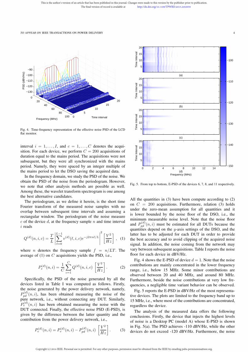
Fig. 4 shows the E-PSD of device d = 1. Note that the noise
contributions are mainly concentrated in the lower frequency
range, i.e., below 15 MHz. Some minor contributions are
observed between 20 and 40 MHz, and around 80 MHz.
Furthermore, beside the noise contributions at very low fre-
quencies, a negligible time variant behavior can be observed.
Fig. 5 reports the E-PSD in dBV/Hz of the most representa-
tive devices. The plots are limited to the frequency band up to
15 MHz, i.e., where most of the contributions are concentrated,
regardless the device.
The analysis of the measured data offers the following
conclusions. Firstly, the device that injects the highest levels
of noise is a Desktop PC (model A) whose E-PSD is shown
in Fig. 5(a). The PSD achieves -110 dBV/Hz, while the other
devices do not exceed -120 dBV/Hz. Furthermore, the noise
This is the author's version of an article that has been published in this journal. Changes were made to this version by the publisher prior to publication.The final version of record is available at http://dx.doi.org/10.1109/TPWRD.2015.2452939
Copyright (c) 2016 IEEE. Personal use is permitted. For any other purposes, permission must be obtained from the IEEE by emailing [email protected].
TO APPEAR ON IEEE TRANSACTIONS ON POWER DELIVERY 5
(a) Frequency (MHz)α = −130 dBV/Hz
Tim
e In
terv
al
0 2 4
2
4
6
8
10
12
14
16
18
20
(b) Frequency (MHz)α = −120 dBV/Hz
0 2 4(c) Frequency (MHz)
α = −110 dBV/Hz
0 2 40
0.1
0.2
0.3
0.4
0.5
0.6
0.7
0.8
0.9
1
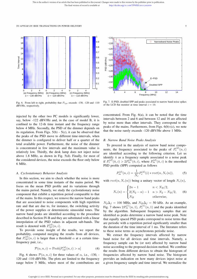
Fig. 6. From left to right, probability that Pcyc exceeds -130, -120 and -110dBV/Hz, respectively.
injected by the other two PC models is significantly lower,
say, below -122 dBV/Hz and, in the case of model B, it is
confined to the 12-th time instant and the frequency range
below 4 MHz. Secondly, the PSD of the dimmer depends on
its regulation. From Figs. 5(b) - 5(c), it can be observed that
the peaks of the PSD move to different time-intervals, when
the dimmer is configured to deliver half or a quarter of the
total available power. Furthermore, the noise of the dimmer
is concentrated in few intervals and the maximum value is
relatively low. Thirdly, the desk lamp does not inject noise
above 1.8 MHz, as shown in Fig. 5(d). Finally, for most of
the considered devices, the noise exceeds the floor only below
6 MHz.
A. Cyclostationary Behavior Analysis
In this section, we aim to check whether the noise is more
concentrated in some time instants of the mains period. We
focus on the mean PSD profile and its variations through
the mains period. Namely, we study the cyclostationary noise
component that exhibit a repetition period comparable to that
of the mains. In this respect, we remove the narrow band peaks
that are associated to noise components with high repetition
rate and that are due to, for instance, the switching activity
of the power supplies or deterministic sinusoidal tones. The
narrow band peaks are identified according to the procedure
described in Section IV-B and they are substituted with a linear
interpolation of the PSD values in adjacent sub-bands. The
result is denoted with P(d)cyc(n, i).
To provide some insight of the results, we report the
probability, computed merging the results from all devices,
that P(d)cyc(n, i) is larger than a threshold α at a certain time-
frequency pair, i.e.,
P(α, n, i) = Prob[P (d)cyc(n, i) > α] (4)
Fig. 6 shows P(α, n, i) for three values of α, i.e., -130, -
120 and -110 dBV/Hz. The plots are limited to the frequency
range below 5 MHz, where most of the contributions are
2 4 6 8 10 12 14
−134
−132
−130
−128
−126
−124
−122
−120
−118
−116
Frequency (MHz)
PS
D (
dBV
/Hz)
Narrowband Noise Peaks
E−PSD
Doubled SPP
Fig. 7. E-PSD, doubled SPP and peaks associated to narrow band noise spikesof the LCD flat monitor at time interval i = 19.
concentrated. From Fig. 6(a), it can be noted that the time
intervals between 2 and 6 and between 12 and 16 are affected
by noise more than other intervals. They correspond to the
peaks of the mains. Furthermore, from Figs. 6(b)-(c), we note
that the noise rarely exceeds -120 dBV/Hz above 1 MHz.
B. Narrow Band Noise Peaks Analysis
To proceed in the analysis of narrow band noise compo-
nents, the frequency associated to the peaks of P(d)e (n, i)
are identified according to the following criterion. Let us
identify n as a frequency sample associated to a noise peak
if P(d)e (n, i) > 2P
(d)m (n, i), where P
(d)m (n, i) is the smoothed
PSD profile (SPP) computed as follows
P (d)m (n, i) =
1
NrP (d)e (i) ∗ rect(n,Nr(n)), (5)
with rect(n,Nr(n)) being a unitary vector of length Nr(n),
Nr(n) =
2n− 1 n < NB/2,
2(N2 − n)− 1 n > N2 −NB/2,
NB otherwise,
(6)
N2∆f = 100 MHz, and NB∆f = 50 kHz. As an example,
Fig. 7 shows 2P(1)m (n, 1), P
(1)e (n, 1) and the peaks identified
by the algorithm. Subsequent frequency samples that are
identified as peaks determine a narrow band noise peak. Note
that equally spaced PSD peaks correspond to noise terms that
are periodic with a repetition period significantly smaller than
the duration of the time interval of 1 ms. The literature refers
to these noise terms as asynchronous periodic noise.
We extract the frequency intervals affected by narrow
band noise for all devices and time intervals. Namely, a
frequency sample can be (or not) affected by narrow band
noise according to the proposed decision method. We combine
the results from different devices to obtain the histogram of
frequencies affected by narrow band noise. The histogram
provides an indication on how many devices inject noise at
a given frequency sample and time interval. We normalize the
This is the author's version of an article that has been published in this journal. Changes were made to this version by the publisher prior to publication.The final version of record is available at http://dx.doi.org/10.1109/TPWRD.2015.2452939
Copyright (c) 2016 IEEE. Personal use is permitted. For any other purposes, permission must be obtained from the IEEE by emailing [email protected].
TO APPEAR ON IEEE TRANSACTIONS ON POWER DELIVERY 6
Frequency (MHz)
Tim
e in
stan
t
2 4 6 8 10 12 14
20
18
16
14
12
10
8
6
4
20.01
0.02
0.03
0.04
0.05
0.06
0.07
0.08
0.09
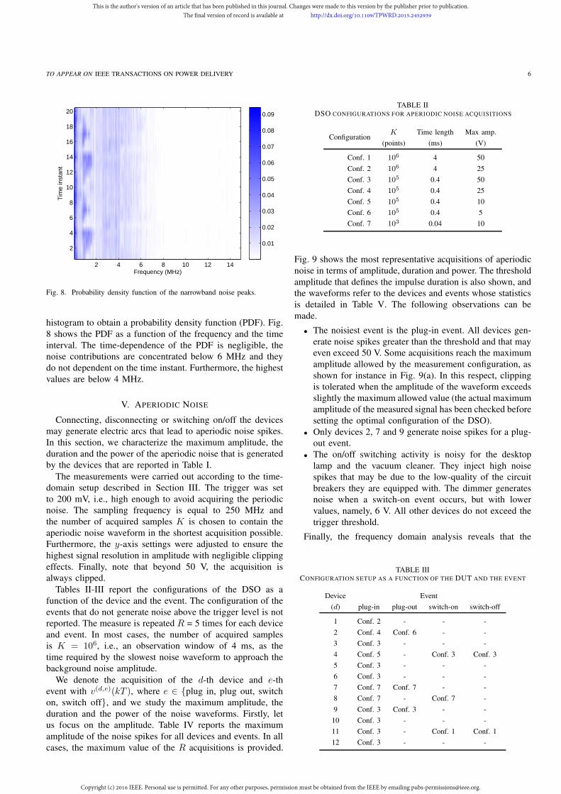
Fig. 8. Probability density function of the narrowband noise peaks.
histogram to obtain a probability density function (PDF). Fig.
8 shows the PDF as a function of the frequency and the time
interval. The time-dependence of the PDF is negligible, the
noise contributions are concentrated below 6 MHz and they
do not dependent on the time instant. Furthermore, the highest
values are below 4 MHz.
V. APERIODIC NOISE
Connecting, disconnecting or switching on/off the devices
may generate electric arcs that lead to aperiodic noise spikes.
In this section, we characterize the maximum amplitude, the
duration and the power of the aperiodic noise that is generated
by the devices that are reported in Table I.
The measurements were carried out according to the time-
domain setup described in Section III. The trigger was set
to 200 mV, i.e., high enough to avoid acquiring the periodic
noise. The sampling frequency is equal to 250 MHz and
the number of acquired samples K is chosen to contain the
aperiodic noise waveform in the shortest acquisition possible.
Furthermore, the y-axis settings were adjusted to ensure the
highest signal resolution in amplitude with negligible clipping
effects. Finally, note that beyond 50 V, the acquisition is
always clipped.
Tables II-III report the configurations of the DSO as a
function of the device and the event. The configuration of the
events that do not generate noise above the trigger level is not
reported. The measure is repeated R = 5 times for each device
and event. In most cases, the number of acquired samples
is K = 106, i.e., an observation window of 4 ms, as the
time required by the slowest noise waveform to approach the
background noise amplitude.
We denote the acquisition of the d-th device and e-th
event with v(d,e)(kT ), where e ∈ plug in, plug out, switch
on, switch off, and we study the maximum amplitude, the
duration and the power of the noise waveforms. Firstly, let
us focus on the amplitude. Table IV reports the maximum
amplitude of the noise spikes for all devices and events. In all
cases, the maximum value of the R acquisitions is provided.
TABLE IIDSO CONFIGURATIONS FOR APERIODIC NOISE ACQUISITIONS
ConfigurationK Time length Max amp.
(points) (ms) (V)
Conf. 1 106 4 50
Conf. 2 106 4 25
Conf. 3 105 0.4 50
Conf. 4 105 0.4 25
Conf. 5 105 0.4 10
Conf. 6 105 0.4 5
Conf. 7 103 0.04 10
Fig. 9 shows the most representative acquisitions of aperiodic
noise in terms of amplitude, duration and power. The threshold
amplitude that defines the impulse duration is also shown, and
the waveforms refer to the devices and events whose statistics
is detailed in Table V. The following observations can be
made.
• The noisiest event is the plug-in event. All devices gen-
erate noise spikes greater than the threshold and that may
even exceed 50 V. Some acquisitions reach the maximum
amplitude allowed by the measurement configuration, as
shown for instance in Fig. 9(a). In this respect, clipping
is tolerated when the amplitude of the waveform exceeds
slightly the maximum allowed value (the actual maximum
amplitude of the measured signal has been checked before
setting the optimal configuration of the DSO).
• Only devices 2, 7 and 9 generate noise spikes for a plug-
out event.
• The on/off switching activity is noisy for the desktop
lamp and the vacuum cleaner. They inject high noise
spikes that may be due to the low-quality of the circuit
breakers they are equipped with. The dimmer generates
noise when a switch-on event occurs, but with lower
values, namely, 6 V. All other devices do not exceed the
trigger threshold.
Finally, the frequency domain analysis reveals that the
TABLE IIICONFIGURATION SETUP AS A FUNCTION OF THE DUT AND THE EVENT
Device Event
(d) plug-in plug-out switch-on switch-off
1 Conf. 2 - - -
2 Conf. 4 Conf. 6 - -
3 Conf. 3 - - -
4 Conf. 5 - Conf. 3 Conf. 3
5 Conf. 3 - - -
6 Conf. 3 - - -
7 Conf. 7 Conf. 7 - -
8 Conf. 7 - Conf. 7 -
9 Conf. 3 Conf. 3 - -
10 Conf. 3 - - -
11 Conf. 3 - Conf. 1 Conf. 1
12 Conf. 3 - - -
This is the author's version of an article that has been published in this journal. Changes were made to this version by the publisher prior to publication.The final version of record is available at http://dx.doi.org/10.1109/TPWRD.2015.2452939
Copyright (c) 2016 IEEE. Personal use is permitted. For any other purposes, permission must be obtained from the IEEE by emailing [email protected].

TO APPEAR ON IEEE TRANSACTIONS ON POWER DELIVERY 7
−20
0
20
Am
plitu
de (
V)
(a)
−50
0
50
Am
plitu
de (
V)
(b)
0 0.5 1 1.5 2 2.5 3 3.5 4−50
0
50
Am
plitu
de (
V)
(c) Time (ms)
Fig. 9. From top to bottom, an example of the acquired impulsive noisegenerated by device 1 during plug in, device 6 during plug in, and device 11during switch off.
aperiodic noise pulses spread over the broadband spectrum,
with PSD levels that exceed -80 dBm/Hz below 10 MHz and
-100 dBm/Hz at 30 MHz. Now, we study the duration of the
noise spikes. Let us define the duration Td as the distance
between the first time instant, i.e., k1T , and the last time
instant, i.e., k2T , for which the absolute value of the noise
exceeds ρ times the maximum. We choose ρ = -10 dB.
Table IV reports the minimum, mean and maximum du-
ration of the aperiodic noise for all operations and devices.
The duration varies significantly even for noise waveforms
generated by the same device and there is no clear indication
about its behavior. To provide a description about the intensity
of the bursty aperiodic noise, we study the power, namely,
P (d,e) =1
ZTd
k2∑
k=k1
T∣
∣
∣v(d,e)(kT )
∣
∣
∣
2
[W ], (7)
where Z = 50 Ω is the input impedance of the DSO. The
evaluation of the noise power enables getting the real nature
of the aperiodic noise components that are made by subsequent
sparse spikes with amplitude exceeding the threshold for short
intervals of time, as shown in Fig. 9(a).
Table IV reports the minimum, mean and maximum power
of the measured noise. The power can be significantly high,
but it refers to noise spikes with very short duration in
time, i.e., less than 200 ns. In any case, the study highlights
the disruptive nature of the impulsive noise. From a PLC
modem manufacturer perspective, this implies, firstly, the need
of protection circuits to preserve the analog front end, and,
secondly, that the received signal is saturated by the impulsive
noise so that the best option is to blank it to avoid corrupting
the demodulation/decoding process.
VI. CONCLUSIONS
An experimental characterization of the PLC noise at the
source has been herein presented. The work is based on the
TABLE IVCHARACTERIZATION OF THE APERIODIC NOISE
Id Ev. Amp. Duration (µs) Power (mW)
(d) (e) (V) min avg max min avg max
1 p. in 25 0.62 1.3e3 3.4e3 18.5 153 471
2p. in 25 0.66 34.4 81 65 1.6e3 3.6e3
p. out 2 14 160 400 0.08 0.44 0.9
3 p. in 50 3.58 94 233 31 1.9e3 4.6e3
4
p. in 10 0.23 9.83 33.5 14.3 432 742
s. on 50 0.17 25.3 86.6 609 6.7e3 2.5e4
s. off 6.8 13.5 249 400 11.8 18 33
5 p. in 50 2.6 9.86 19.5 189 4.3e3 8.2e3
6 p. in 50 1.28 12.2 27.4 1.2e3 2.4e3 5.1e3
7p. in 5 0.02 0.04 0.06 12.2 92.6 179
p. out 5.8 0.05 1.95 4 2.12 42 143
8p. in 3.84 0.03 0.46 2.1 0.54 56.2 87.2
s. on 3.52 4e-3 2.26 4 0.36 88.3 310
9p. in 50 0.58 15.5 36.5 186 3.2e3 7.2e3
p. out 41.6 1.86 196 400 11.6 83.5 287
10 p. in 50 0.2 93.6 272 76.7 6.5e3 2.2e4
11
p. in 40.4 0.06 20.9 44.5 23.6 5.5e3 1.5e4
s. on 50 354 395 443 54.8 637 1.1e3
s. off 50 201 1.3e3 3.1e3 575 851 1.2e3
12 p. in 50 1.64 21.2 96.3 30.1 5.4e3 7.6e3
results of a measurement campaign that addressed the noise
generated by a number of household appliances.
Both the noise generated during the normal-mode operating
condition and during transients has been analyzed. The former
is generated by the appliances during their normal activity, i.e.,
when they are switched on and running. The latter is generated
when devices are switched on/off or they are plugged in/out.
Concerning the normal-mode operation noise, we have firstly
studied the cyclostationary behavior. Then, we have carried
out an analysis of the frequencies where narrow band noise
peaks are concentrated. The study has revealed the following
findings.
• The noisiest device is a desktop PC that injects noise
whose power spectral density exhibits peaks of up to
−110 dBV/Hz, although below 4 MHz.
• In general, the noise shows a time variant behavior, with
a period equal to the mains period.
TABLE VCHARACTERISTIC OF THE NOISE WAVEFORMS
Fig.Device Event Max. Amp. Duration Power
(d) (e) (V) (µs) (mW)
9(a) 1 plug in 25 3.4e3 27.4
9(b) 6 plug in 50 24.1 5.1e3
9(c) 11 switch off 50 3.1e3 575
This is the author's version of an article that has been published in this journal. Changes were made to this version by the publisher prior to publication.The final version of record is available at http://dx.doi.org/10.1109/TPWRD.2015.2452939
Copyright (c) 2016 IEEE. Personal use is permitted. For any other purposes, permission must be obtained from the IEEE by emailing [email protected].
TO APPEAR ON IEEE TRANSACTIONS ON POWER DELIVERY 8
• Within the mains period, the noisiest time intervals are
associated to time instants when the mains signal (in
absolute value) reaches a peak.
• The narrow band noise is present below 4 MHz.
Finally, we have targeted the aperiodic noise that is gen-
erated during switching transients and we have shown that
the aperiodic noise spikes may exhibit very large amplitudes,
i.e., greater than 50 V, and they may last up to 4 ms, but
with a low duty cycle. In fact, in general, the average power
is small, in the order of fractions of Watts. Nevertheless, in
all cases, the aperiodic noise is disruptive and blanking the
received samples affected by such impairment is a valuable
solution when combined with channel coding.
From a regulatory perspective, this study has highlighted
that several devices inject a great deal of noise so that more
PLC friendly norms should be developed by imposing more
stringent EMC limits to power devices.
REFERENCES
[1] E. Biglieri, “Coding and modulation for a horrible channel,” IEEE
Commun. Mag., vol. 41, no. 5, pp. 92–98, May 2003.[2] M. Gotz, M. Rapp, and K. Doster, “Power line channel characteristics
and their effect on communication system design,” IEEE Commun. Mag.,vol. 42, no. 4, pp. 78–86, Apr. 2004.
[3] T. Esmailian, F. R. Kschischang, and P. Glenn Gulak, “In-building powerlines as high-speed communication channels: Channel characterizationand a test channel ensemble,” Intern. J. of Commun. Syst., vol. 16, no. 5,pp. 381–400, Jun. 2003.
[4] R. Hashmat, P. Pagani, and T. Chonavel, “Mimo communications forinhome plc networks: Measurements and results up to 100 mhz,” inProc. IEEE Int. Symp. Power Line Commun. and Its App. (ISPLC), Apr.2010, pp. 120–124.
[5] D. Middleton, “Statistical-physical models of electromagnetic interfer-ence,” IEEE Trans. Electromagn. Compat., vol. 19, no. 3, pp. 106–127,Aug. 1977.
[6] H. Meng, Y. L. Guan, and S. Chen, “Modeling and analysis of noiseeffects on broadband power-line communications,” IEEE Trans. Power
Del., vol. 20, no. 2, pp. 630–637, Apr. 2005.[7] M. Katayama, T. Yamazato, and H. Okada, “A mathematical model of
noise in narrowband power line communication systems,” IEEE J. Sel.
Areas Commun., vol. 24, no. 7, pp. 1267–1276, Jul. 2006.[8] J. A. Cortes, L. Dıez, F. J. Canete, and J. J. Sanchez-Martınez, “Anal-
ysis of the indoor broadband power-line noise scenario,” IEEE Trans.
Electromagn. Compat., vol. 52, no. 4, pp. 849–858, Nov. 2010.[9] M. Zimmermann and K. Dostert, “Analysis and modeling of impulsive
noise in broad-band powerline communications,” IEEE Trans. Electro-
magn. Compat., vol. 44, no. 1, pp. 249–258, Feb. 2002.[10] F. Gianaroli, F. Pancaldi, E. Sironi, M. Vigilante, G. M. Vitetta, and
A. Barbieri, “Statistical modeling of periodic impulsive noise in indoorpower-line channels,” IEEE Trans. Power Del., vol. 27, no. 3, pp. 1276–1283, Jul. 2012.
[11] M. H. L. Chan and R. W. Donaldson, “Amplitude, width, and interarrivaldistributions for noise impulses on intrabuilding power line communica-tion networks,” IEEE Trans. Electromagn. Compat., vol. 31, no. 3, pp.320–323, Aug. 1989.
[12] L. di Bert, P. Caldera, D. Schwingshackl, and A. M. Tonello, “On noisemodeling for power line communications,” in Proc. IEEE Int. Symp. on
Power Line Commun. and Its App. (ISPLC), Apr. 2011, pp. 283–288.[13] M. Tlich, H. Chaouche, A. Zeddam, and P. Pagani, “Novel approach
for plc impulsive noise modelling,” in Proc. IEEE Int. Symp. on Power
Line Commun. and Its App. (ISPLC), Mar. 2009, pp. 20–25.[14] J. Khangosstar, L. Zhang, and A. Mehboob, “An experimental analysis
in time and frequency domain of impulse noise over power lines,” inProc. IEEE Int. Symp. on Power Line Commun. and Its App. (ISPLC),Apr. 2011, pp. 218–223.
[15] M. Tlich, H. Chaouche, A. Zeddam, and F. Gauthier, “Impulsive noisecharacterization at the source,” in Proc. IFIP Wireless Days WD’08,Nov. 2008, pp. 1–6.
[16] J. J. Lee, S. J. Choi, H. M. Oh, W. T. Kee, K. H. Kim, and D. Y. Lee,“Measurements of the communications environment in medium voltagepower distribution lines for wide-band power line communications,” inProc. IEEE Int. Symp. Power Line Commun. and Its App. (ISPLC), Apr.2004, pp. 69–74.
[17] M. Antoniali and A. M. Tonello, “Measurement and characterizationof load impedances in home power line grids,” IEEE Trans. Instrum.
Meas., vol. 63, no. 3, pp. 548–556, Mar. 2014.[18] M. Antoniali, A. M. Tonello, and F. Versolatto, “A study on the optimal
receiver impedance for snr maximization in broadband plc,” Journal of
Electrical and Computer Engineering, vol. 2013, pp. 1–13, 2013.
Massimo Antoniali received the B.Sc. degree inelectrical engineering (2007), the M.Sc. degree inelectrical engineering (2009, summa cum laude) andthe Doctoral Degree in industrial and informationtechnology (2013), all from the of University ofUdine, Italy. In 2013 he joined SMS Concast Italia.His research interests are in the field of data com-munications and communication systems character-ization. He received two best student paper awardsat the IEEE International Symposium on Power LineCommunications (ISPLC) in 2011 and in 2013.
Fabio Versolatto (SM10) received the B.Sc. degree(2007) and the M.Sc. degree (2009) in electricalengineering (both summa cum laude), and the Ph.D.degree in industrial and information engineering(2013), from the University of Udine, Udine, Italy.He was a member of the Wireless and Power LineCommunications Lab at the University of Udineuntil 2015. Currently, he is with Innova, Italy. Hisresearch interests are in the field of channel mod-eling for power line communications and digitalcommunication algorithms. He is member of the
IEEE Technical Committee on Power Line Communications and he has beenTPC member of IEEE ISPLC 2014. He received the best student paper awardpresented at IEEE ISPLC 2010.
Andrea M. Tonello (M00, SM12) obtained the Lau-rea degree (1996, summa cum laude) and the Doctorof Research degree in electronics and telecommuni-cations (2003) from the University of Padova, Italy.From 1997 to 2002 he was with Bell Labs LucentTechnologies firstly as a Member of Technical Staffand then as a Technical Manager at the AdvancedWireless Technology Laboratory, Whippany, NJ andthe Managing Director of the Bell Labs Italy di-vision. In 2003 he joined the University of Udine,Italy, where he became Aggregate Professor in 2005
and Associate Professor in 2014. Herein, he founded the Wireless and PowerLine Communication Lab. He also founded WiTiKee, a spinoff company inthe field of telecommunications for the smart grid. Currently, he is the Chair ofthe Embedded Communication Systems group at the University of Klagenfurt,Austria. Dr. Tonello received the Lucent Bell Labs Recognition of Excellenceaward (1999), the Distinguished Visiting Fellowship from the Royal Academyof Engineering, UK (2010) and the Distinguished Lecturer Award by the IEEEVehicular Technology Society (2011-13 and 2013-15). He also received (as co-author) five best paper awards. He is the Chair of the IEEE CommunicationsSociety Technical Committee on Power Line Communications. He serves anAssociate Editor for the IEEE Transactions on Communications (since 2012)and IEEE Access (since 2013). He was the Chair of IEEE ISPLC 2011 andIEEE SmartGridComm 2014.
This is the author's version of an article that has been published in this journal. Changes were made to this version by the publisher prior to publication.The final version of record is available at http://dx.doi.org/10.1109/TPWRD.2015.2452939
Copyright (c) 2016 IEEE. Personal use is permitted. For any other purposes, permission must be obtained from the IEEE by emailing [email protected].


