econstorMake Your Publication Visible

A Service of

zbwLeibniz-InformationszentrumWirtschaftLeibniz Information Centrefor Economics

van Aarle, Bas

Working Paper

Secular Stagnation: Insights from a New KeynesianModel with Hysteresis Effects

CESifo Working Paper, No. 5797

Provided in Cooperation with:Ifo Institute – Leibniz Institute for Economic Research at the University ofMunich

Suggested Citation: van Aarle, Bas (2016) : Secular Stagnation: Insights from a New KeynesianModel with Hysteresis Effects, CESifo Working Paper, No. 5797

This Version is available at:http://hdl.handle.net/10419/130410

Standard-Nutzungsbedingungen:

Die Dokumente auf EconStor dürfen zu eigenen wissenschaftlichenZwecken und zum Privatgebrauch gespeichert und kopiert werden.

Sie dürfen die Dokumente nicht für öffentliche oder kommerzielleZwecke vervielfältigen, öffentlich ausstellen, öffentlich zugänglichmachen, vertreiben oder anderweitig nutzen.

Sofern die Verfasser die Dokumente unter Open-Content-Lizenzen(insbesondere CC-Lizenzen) zur Verfügung gestellt haben sollten,gelten abweichend von diesen Nutzungsbedingungen die in der dortgenannten Lizenz gewährten Nutzungsrechte.

Terms of use:

Documents in EconStor may be saved and copied for yourpersonal and scholarly purposes.

You are not to copy documents for public or commercialpurposes, to exhibit the documents publicly, to make thempublicly available on the internet, or to distribute or otherwiseuse the documents in public.

If the documents have been made available under an OpenContent Licence (especially Creative Commons Licences), youmay exercise further usage rights as specified in the indicatedlicence.

www.econstor.eu

Secular Stagnation: Insights from a New Keynesian Model with Hysteresis Effects

Bas van Aarle

CESIFO WORKING PAPER NO. 5797 CATEGORY 6: FISCAL POLICY, MACROECONOMICS AND GROWTH

MARCH 2016

An electronic version of the paper may be downloaded • from the SSRN website: www.SSRN.com • from the RePEc website: www.RePEc.org

• from the CESifo website: Twww.CESifo-group.org/wp T

ISSN 2364-1428

CESifo Working Paper No. 5797

Secular Stagnation: Insights from a New Keynesian Model with Hysteresis Effects

Abstract To analyse the most important aspects of the Secular Stagnation hypothesis, this paper considers the effects of hysteresis in potential output in a New-Keynesian model that is extended with endogenous potential output. To do so, a number of simulations of relevant scenarios is undertaken. It is demonstrated that extending the New-Keynesian model with hysteresis has a number of crucial implications for macro-economic adjustment and macro-economic management. It is indicated how the model can contribute to a better understanding of a number of important elements of the Secular Stagnation hypothesis.

JEL-Codes: E310, E430, E620, H620.

Keywords: potential output hysteresis, monetary policy, fiscal policy.

Bas van Aarle Leuven Center for Irish Studies

Janseniusstraat 1 Belgium – 3000 Leuven

bas.vanaarle@econ.kuleiven.be

February 25, 2016 I am grateful for the comments made by two anonymous referees.

1. Introduction

In recent years, many countries recovered only very slowly from the Great Recession that resultedfrom the Global Financial Crisis of 2008. In most European countries e.g., output and employmentgrowth has been small if positive at all and output and employment levels are struggling to reachpre-crisis levels. Policymakers and economists indeed have a difficult time in providing a completeexplanation for the observed shallowness of recovery and in finding the most effective policy responsesin these difficult conditions.

A recent debate -”the Secular Stagnation hypothesis”- seeks to provide a better understandingof this very slow recovery. Summers (2014) summarizes this debate as follows: ”The new SecularStagnation hypothesis responds to recent experience and the manifest inadequacy of conventionalformulations by raising the possibility that it may be impossible for an economy to achieve fullemployment, satisfactory growth and financial stability simultaneously simply through the operationof conventional monetary policy. It thus provides a possible explanation for the dismal pace ofrecovery in the industrial world and also for the emergence of financial stability problems as anincreasingly salient concern.”

In the Secular Stagnation scenario the output effects of the crisis persist, and actual output levelsdo not seem to return to (pre-crisis) potential output levels for a protracted period. One possibleexplanation for this phenomenon is the hysteresis hypothesis: the observed Secular Stagnation couldreflect a permanent drop in potential output and employment as a consequence of the endogenousadjustment effects that have been triggered by the Financial Crisis. Hysteresis effects of currentoutput on future potential output operate through the effect that a current reduction in investmenthas on future capital and through the effect of current unemployment on worker skills and laborforce attachment. Hysteresis is not easy to prove: what adds to the difficulties in the analysis ofhysteresis, is that potential output is an unobservable variable: it is actually very difficult to pindown in the real world. In fact, it can not be excluded that potential output had been overestimatedin the boom-period before the financial crisis.

An other important feature of the Secular Stagnation debate is the possibility of excess savingsthat would require real interest rates to be very low or even negative for an extended time. In a recentnarrative policy study on secular stagnation coordinated by Teulings and Baldwin (2014), a numberof crucial demand (adverse demographic trends, fiscal stringency, monetary policy impotence dueto zero lower bound, over-indebtedness causing excess-saving and a ’balance-sheet’ recession) andsupply factors (lack of innovation, slowdown in efficiency, sclerotic factors in the labour market) areidentified that could explain the Secular Stagnation.

To analyse the most important aspects of the Secular Stagnation hypothesis, this paper considersthe effects of hysteresis in potential output in a New-Keynesian model that is extended with hysteresisin potential output. To do so, a number of simulations of relevant scenarios is undertaken. It isdemonstrated that such an extension of a standard New Keynesian model with hysteresis has anumber of crucial implications for macro-economic adjustment and macro-economic management. Itis indicated how the model can indeed help us to understand a number of important elements of theSecular Stagnation hypothesis.

This paper is organised in as follows: Section 2 discusses the Secular Stagnation Hypothesis,focusing on the effects of the financial crisis and its aftermath on potential output. Section 3 pro-vides a New-Keynesian analytical framework that is extended with hysteresis effects. Section 4 usesnumerical simulations of a stylised example to illustrate the workings of the model and relates theresults to the context of Europe’s very slow recovery crisis and the current discussions about fiscal

2

management in the Euro Area and structural reform policies. Section 4 concludes.

2. The financial crisis, (potential) output and the Secular Stagnation Hypothesis

The very sluggish output and employment recovery in Europe and elsewhere from the financialcrisis and ensuing recession, has led economists and policy makers increasingly to consider the pos-sibility that the Great Recession is not an ordinary recession from which the economy could recoverrelatively quickly. Instead, they argue, this period of very slow growth may actually point at deeper,structural problems that prevent a quick recovery so far. In several studies on the recent financialcrisis and Great Recession, it has been pointed out that in many OECD countries a substantialpotential output loss (in the order of 5 to 10 percent of GDP) occurred as a result of the Great Re-cession. European Commision (2009), OECD (2009), Furceri and Mourouganne (2012), Ball (2014),Ollivaud and Turner (2014), Anderton et. al. (2014) are all detailed empirical studies that seek toestimate effects of the financial crisis on potential output and employment finding evidence for sucha substantial loss in potential output.

It is important to understand how the financial crisis could lead to such a drop in the (actual andpotential) output level and/or growth rate and how persistent such a drop could be. The adverseeffects on potential output would result from the impact of the financial crisis on its three maindeterminants: the stock of capital, the amount of labour and technology, as reflected in Total FactorProductivity (TFP). The financial crisis and recession have reduced investment in new capital andtechnology: investment opportunities declined and credit from banks became more scarce as banksbecame more concerned about credit risk. The recession has also reduced opportunities in the labourmarket. There is the accompanying risk that the increase in unemployment as a result of the crisisturns into an increase in structural unemployment as worker skills deteriorate with longer spells ofunemployment.

The ”hysteresis hypothesis” assumes that the economy retains a memory of the shocks associatedwith recessions, implying path-dependence in macro-economic adjustments. Hysteresis has pervasiveimplications for macroeconomic adjustment and policy. It opens up the possibility that temporaryshocks may have permanent effects in the economy, in particular a permanent drop in the levelof potential output and an increase in structural unemployment. Hysteresis results from capitalscrapping and labour market rigidities (including the well-known ”insider/outsider” conflicts), thatprevent/discourage many unemployed workers to re-enter employment again after the recession. Thehigh rate of joblessness and long duration of joblessness, discourages workers further and will resultin a permanent destruction of human capital when discouraged workers exit their labour marketsearch.

A significant literature on hysteresis resulted from the experiences of the 1970s and 1980s whenafter the first and second Oil Crisis and ensuing recessions, unemployment displayed the ”ratchet-effect” that is characteristic for hysteresis. In both cases, unemployment failed to drop to the levelbefore the recession and stayed stubbornly high.1 Clearly countries are likely to differ in the degree towhich hysteresis is affecting the economy at a certain moment. These differences reflect the underlying

1See e.g. Bruno and Sachs (1985), Blanchard and Summers (1986), (1987) and (1988), and Lindbeck and Snower(1986) on the hysteresis experiences of associated with the first and second Oil Crisis of the 1970s and 1980s. Therelated empirical debate about unit roots in output (Stock and Watson (1986) and Diebold and Rudebusch (1987))also dates back to the same period.

3

institutional settings, the impact of various shocks and the policy reactions. Some countries wereless affected e.g. by the Great Recession than others for whom hysteresis could be a serious concern.

Another theoretical literature that is also of some relevance for our analysis studies the effect ofoutput gap uncertainty on monetary and fiscal policy management, see e.g. Ehrmann and Smets(2003). This literature takes as a starting point the observation that policy makers face incompleteinformation about current economic conditions, and in particular about potential output. Potentialoutput is an unobservable variable, resulting in uncertainty about its actual adjustment. As a result,policy makers have to form estimations/expectations about the actual level of potential output (andits growth rate) and consequently of the actual output gap. As a result of this uncertainty, potentialoutput and the output gap are often subject to significant revisions, especially during crisis periods.This uncertainty makes it difficult to evaluate the adequateness of current monetary and fiscal policyfrom the perspective of business cycle stabilization. This literature concludes that more potentialoutput uncertainty requires more caution in setting policies as the possibility of policy errors inincreased. This literature, however, focuses on output gap uncertainty and does not consider thepossibility of hysteresis as a source of endogenous business cycle fluctuations.2

A consequence of the Financial Crisis and Great Recession is higher uncertainty surroundingestimates of potential output compared to the previous decade of Great Moderation. This uncertaintyis evident in the continued downward revisions in the estimates of potential output growth for almostall OECD countries during the Great Recession since 2008. It is not therefore not clear in the wake ofthe observed very weak recovery of output and employment, what are the most realistic expectationsconcerning potential output and employment in the near and more distant future. This dependsalso on which scenario is most likely concerning the impact the financial crisis has had on potentialoutput growth.

Three possible scenarios concerning the effects of the financial crisis on the potential output leveland its growth-rate in the long-run are distinguished in Figure 1. First is one-off changes in the levelof GDP without a change in long-run potential output level and its growth rate (green lines). Inthis scenario, after the Great Recession, economic recovery will eventually bring the economy againon the pre-crisis growth path in the long run. While the recession could be deep and persistent,this scenario would imply that the output loss is eventually recovered. Second is the possibility of apermanent decline in the potential output level without a change in the long-run potential growthrate (blue lines). This scenario is equivalent to hysteresis in output and unemployment. Third, is apermanent drop in the potential output level and long-run potential growth rate, resulting in a formof ”super-hysteresis” (red lines).

In mainstream macroeconomic models, hysteresis is not considered given the complexities itentails in terms of theory, empirical estimation and policy analysis. Hysteresis implies that a tem-porary shock has permanent effects so that the economy does not return to the initial steady-statebut adjusts to a new -endogenous- steady-state, an aspect that we will demonstrate in detail in thenumerical analysis. In a similar vein, empirical analysis is also complicated by hysteresis: in case ofhysteresis, variables contain a unit-root so that the second and higher order moments of variables

2The standard New Keynesian models and their more worked out DSGE variants rely on exogenous business cyclefluctuations in the sense that economic adjustments are the result of various types of shocks that hit the economy andtransmit themselves through various transmission channels -exogenous transmission of shocks in other words- afterwhich the economy returns to steady-state. In case of endogenous fluctuations like in case of hysteresis, shocks alsoimply that the transmission of shocks is endogenous since the steady-state itself is also affected by the temporaryshock.

4

Figure 1: Effects of the financial crisis on the level and growth rate of potential output (hypothetical potential andactual output series).

are not defined. Estimation and measurement errors of the true potential output/output gap willtranslate in policy errors: in particular policy makers are faced with the uncertainty whether actualoutput and inflation adjustment reflects the occurrence of potential output shocks or is caused byother shocks: demand shocks, mark-up shocks etc. E.g. an overestimation of potential output impliesan overestimation of the output gap in times of recession, inducing policy makers to policies thatcould be inflationary in the short-run and the fiscal stance is likely to be to lax from the perspectiveof the true potential output. In a similar manner, in case of underestimation of potential output,macroeconomic policies could be too restrictive and risk to contribute to deflationary pressures.

3. The Analytical Framework

Our analytical framework follows the baseline New Keynesian model as a description of the behaviorof macroeconomic variables (e.g., Woodford (2003), Gali (2008)). The adjustment of output, inflationand interest rates is described by the dynamic IS curve (1), the (hybrid) New Keynesian Phillipscurve (2), and dynamic Taylor rules that characterise monetary policy (3), and fiscal policy (4). Inaddition to these standard equations, we add dynamics of potential output (5) as we would like toanalyse the consequences of hysteresis in potential output. The dynamic IS curve summarizes theaggregate goods demand in the economy:

yt = ωEyt+1 + (1 − ω)yt−1 − σ(it − Eπt+1 − rnt ) + gt + εyt (1)

in which y denotes real output, i the short-term nominal interest rate, π the rate of inflation in thegeneral price level, rn the natural or equilibrium real interest rate, g net government spending, εy isan aggregate demand shock. The subscript t refers to time, E is the expectations operator.

In this reduced form output depends on past output, expected future output, the real interestrate (expressed as a deviation from the natural real interest rate), net government spending, and ademand shock . The backward-looking component in the IS curve results the fraction of consumersthat are backward-looking because of habit formation in consumption decisions (or because they face

5

credit constraints). The forward-looking part is produced by rational, inter-temporally maximizingagents that apply the principles of optimal consumption-smoothing.

All macroeconomic shocks in the model -demand shocks (εy), cost-push shocks (επ), monetaryshocks (εi), fiscal shocks (εg), potential output shocks (εy), natural interest rate shocks, (εrn)- areassumed to follow stationary AR(1) processes, εjt = νjε

jt−1 + vjt where all innovations are white noise

innovations, and all innovations are assumed to be contemporaneously uncorrelated.3

Inflation adjusts according to a hybrid New Keynesian Phillips-curve which contain elementsof both forward and backward-looking price setting. In addition, the output gap as a measure ofdemand-pull inflation, and mark-up shocks επ affect inflation:

πt = βEπt+1 + (1 − β)πt−1 + κxt + επt (2)

The output gap xt = yt − yt measures the distance between actual output and potential output, yt.A Taylor rule with partial adjustment will be used as an approximation of monetary policy

decisions in the economy. The monetary authority is assumed to set the short-term nominal interestrate, in response to movements in inflation and the output gap. ρi measures inertia in interest rateadjustment, χπ and χx are reaction coefficients to inflation and output gap, π is an inflation target.

it = ρiit−1 + (1 − ρi)(rnt + π + χππt + χxxt) + εit (3)

The feedback on inflation and output gap are standard arguments in the Taylor rule, the weightsgiven to both objectives are given by the reaction coefficients χπ and χx. The degree of instrumentsmoothing is measured by ρi, where 0 < ρi < 1. If ρi goes to zero the original Taylor rule, whichignores instrument-smoothing, is obtained. If ρi goes to one, monetary policy is increasingly smoothedover time.

Fiscal policy is given by a Taylor rule as well:

gt = ρggt−1 + (1 − ρg)(g − µxt) + εgt (4)

according to which net government spending responses to movements in the output gap. ρg measuresinertia budgetary adjustment, g is a net government spending target, εg denotes a budgetary shock.

The standard New Keynesian model assumes potential output to be constant (possibly subjectto stochastic shocks) in order to focus on short-run fluctuations in output as a result of shocksto consumer preferences, labour supply shocks, firms’ mark-up shocks, technological shocks andpolicy shocks. For our purpose it is more useful to consider endogenous adjustment of potentialoutput, reflecting the possibility of hysteresis. The standard New Keynesian model does not considerhysteresis, therefore we introduce endogenous potential output into the model in the following way:

yt = ρyyt−1 + αyt−1 + εyt (5)

Potential output depends on past potential output, actual output and potential output innovations,εy. In case α=0 the model reduces to the standard New Keynesian model with exogenous potential

3Strictly speaking, in the hysteresis case, these shocks need to be considered/implemented as deterministic processes,given that the mean and variance of the output and potential output variables are not defined in the hysteresis case,as hysteresis implies that the various shocks can have permanent effects on the mean of potential and actual output,viz. potential and actual output are following random walks.

6

output, in case α=1, potential output displays hysteresis. In the intermittent case, 0 < α < 1,potential output dynamics are persistent. We will consider a value α=0.5 to study this intermittentcase.

In their analysis on the impact of potential output persistence on optimal monetary policy, Kien-zler and Schmid (2014) consider values of α between 0 and 0.5 and demonstrate the need for additionalmonetary policy activism (in terms of reacting to temporary shocks) in the presence of potential out-put gap persistence. The intuition of this outcome is found in the stronger effects of shocks (andtherefore of societal welfare in terms of output and inflation volatility), the stronger is the persistencein potential output. They refer to these cases with potential output persistence as hysteresis. Thisseems somewhat confusing. As we will see it is more useful to reserve hysteresis for the case α=1,and persistent potential output for to the case where 0 < α < 1, since both cases are fundamentallydifferent in the resulting adjustment dynamics.

4. Numerical Results

In this section, we simulate a number of relevant scenarios for the New-Keynesian hysteresis model(1)-(5). We consider the effects of: (i) a temporary negative demand shock, (ii) a one-off positivecost-push shock, (iii) a temporary negative shock to the natural interest rate, (iv) varying the degreeof fiscal stabilization and, (v) a temporary negative demand shock that is accompanied by structuralreform effort. The simulations assume the set of baseline model parameters presented in Table 1.These parameters were not empirically estimated but chosen based on plausibility and their usefulnessas a baseline. A caveat therefore applies: small changes in this set of baseline parameters will leadto quantitative changes in outcomes, bigger changes may also change outcomes qualitatively.

ω 0.5 π 0 ρy 0.5 νεy 0.25σ 1.0 χπ 1.5 α [0,0.5,1] νεg 0.0β 0.5 χx 0.5 νεy 0.5 νεrn 0.5κ 0.1 ρg 0.5 νεπ 0.0 g 0ρi 0.5 µ 0.5 νεi 0.0

Table 1: Baseline parameter set.

4.1. Effects of a temporary demand shock

A crucial implication of hysteresis is the possibility that temporary shocks can have permanent ef-fects on output and unemployment (through the hysteresis effects on potential output): in the longoutput is at a lower level than it would have been in the absence of the shock. We can illustrate ofthe workings of hysteresis in our model by considering the impact and transmission of a temporarydemand shock. Figure 2 displays the effects of a negative demand shock in period 1 and its sub-sequent transmission in (potential), output, output gap, inflation, interest rate and net governmentspending. The blue line gives adjustment in the case of the standard New Keynesian model withouthysteresis (α = 0), the green lines give adjustment in the persistent potential output case (α = 0.5),and red lines give the adjustment under hysteresis, (α = 1).

The implications of hysteresis are quite clearly demonstrated by this example. While in thestandard New Keynesian model and in the persistent potential output case, output returns to the

7

output

0 5 10 15 20 25 30

-15

-10

-5

0

x 10-3

time

alpha=0 alpha=0.5 alpha=1

potential output

0 5 10 15 20 25 30

-15

-10

-5

0

x 10-3

time

alpha=0 alpha=0.5 alpha=1

output gap

0 5 10 15 20 25 30

-15

-10

-5

0

x 10-3

time

alpha=0 alpha=0.5 alpha=1

inflation

0 5 10 15 20 25 30

-2.5

-2

-1.5

-1

-0.5

0

x 10-3

time

alpha=0 alpha=0.5 alpha=1

interest rate

0 5 10 15 20 25 30-7

-6

-5

-4

-3

-2

-1

0

1x 10

-3

time

alpha=0 alpha=0.5 alpha=1

net government spending

0 5 10 15 20 25 30-1

0

1

2

3

4

5x 10

-3

time

alpha=0 alpha=0.5 alpha=1

Figure 2: Effects of a temporary negative demand shock.

initial output level after a temporary recession, it fails to do so in the hysteresis case. The reason thatit fails to do so is exactly the permanent drop in potential output in the hysteresis case. Given theNew-Keynesian Phillips curve, the output gap is closed and inflation disappears once the temporaryshock has faded out. Active monetary and fiscal policies in form of lower interest rates and higher netgovernment spending contribute to the adjustment dynamics, but cannot prevent the long-run dropin (potential) output in the hysteresis cases. In case of hysteresis in potential output, the temporaryshock is detrimental in the long run and active stabilization policies are desirable as they contributecushioning the initial impacts of shocks and their subsequent transmissions in the wider economy.

4.2. Effects of a temporary cost-push shock

Mark-up/cost-push like oil price or wage cost shocks are another important sources of macroeco-nomic fluctuations. Mark-up shocks in the real world and in the New-Keynesian, create even morecomplications for policy makers than demand shocks since inflation is only indirectly controlled bythe influence of active policies on the output gap. In case mark-up shocks occur, the monetary policy

8

maker is facing a dilemma between actively stabilizing output by setting lower interest rates (and toaccept the higher inflation resulting from expansionary monetary policy) or to stabilise inflation byraising interest rates (and accept the resulting temporary output loss). Figure 3 considers the effectsof one-off one percent positive cost-push shock in period 1.

output

0 5 10 15 20 25 30

-0.04

-0.03

-0.02

-0.01

0

time

alpha=0 alpha=0.5 alpha=1

potential output

0 5 10 15 20 25 30

-0.04

-0.03

-0.02

-0.01

0

time

alpha=0 alpha=0.5 alpha=1

output gap

0 5 10 15 20 25 30-15

-10

-5

0

x 10-3

time

alpha=0 alpha=0.5 alpha=1

inflation

0 5 10 15 20 25 30

0

5

10

15

x 10-3

time

alpha=0 alpha=0.5 alpha=1

interest rate

0 5 10 15 20 25 30-2

0

2

4

6

8

10

12

x 10-3

time

alpha=0 alpha=0.5 alpha=1

net government spending

0 5 10 15 20 25 30-1

0

1

2

3

4

x 10-3

time

alpha=0 alpha=0.5 alpha=1

Figure 3: Effects of a one-off positive cost-push shock.

The mark-up shock creates stagflation: output drops and inflation increases. In the no-hysteresiscase, the New-Keynesian model displays a convergence to the initial output level over time sincepotential output is unaffected. Monetary and fiscal stabilization policies are relatively ineffective,they just moderate inflation and/or output during the adjustment to the initial output level. In caseof hysteresis, adjustment is different as the economy would settle for a lower potential and actualoutput level due to the hysteresis channel. This increases also significantly the potential role forfiscal and monetary stabilization policies: these policies can contribute to moderating the eventualactual and potential output drop as a result of the temporary shock.

9

4.3. Effects of a shock to the natural rate of interestThe natural or equilibrium rate of interest is defined as the interest rate that would produce anaggregate demand equal to the natural rate of output, the rate of output that prevails if pricesare fully flexible. The natural rate of interest in other words represents a neutral monetary policystance. According to Summers (2014) and other observers, one factor that has also been connectedto the Secular Stagnation hypothesis is a decline in the equilibrium real rate of interest. This dropreflects imbalances between global savings (which have increased) and global investment (which hasdecreased as a that result of the Financial Crisis). In cases like these where the natural rate ofinterest and inflation are approaching zero, conventional monetary policy is increasingly impotent tostimulate the economy since that would require setting interest rates below zero. Figure 4 demon-strates the effects in the New-Keynesian model with hysteresis of a temporary one percent negativeshock to the natural rate of interest rnt in period 1.

output

0 5 10 15 20 25 30

-15

-10

-5

0

x 10-3

time

alpha=0 alpha=0.5 alpha=1

potential output

0 5 10 15 20 25 30

-15

-10

-5

0

x 10-3

time

alpha=0 alpha=0.5 alpha=1

output gap

0 5 10 15 20 25 30-15

-10

-5

0

x 10-3

time

alpha=0 alpha=0.5 alpha=1

inflation

0 5 10 15 20 25 30-3

-2.5

-2

-1.5

-1

-0.5

0

0.5x 10

-3

time

alpha=0 alpha=0.5 alpha=1

interest rate

0 5 10 15 20 25 30-0.025

-0.02

-0.015

-0.01

-0.005

0

time

alpha=0 alpha=0.5 alpha=1

net government spending

0 5 10 15 20 25 30-1

0

1

2

3

4x 10

-3

time

alpha=0 alpha=0.5 alpha=1

Figure 4: Effects of a temporary negative natural interest rate shock.

The simulations of the model of this shock are in line with the intuitions of Summers (2014) and

10

other observers. The drop in the natural rate of interest provokes a recessionary and deflationaryspiral. In the no-hysteresis regime, the economy recovers quite quickly also helped by expansionarymonetary and fiscal policies; in the persistent potential output case the adjustment is similar butmore gradual. In the hysteresis case, outcomes are more problematic as potential output is affectedin the long run by this temporary shock. The hysteresis scenario in the model in other words is quitein line with the assertions of Summers and others on the Secular Stagnation hypothesis.

4.4. Effects of changing the strength of fiscal stabilization

The presence of hysteresis would a priori seem to strengthen the case for monetary and/or fiscalstabilization policies. In the no-hysteresis case (and the persistent potential output case with somedelay), the economy will return to the original level of output when the shocks have been absorbed.Stabilization policies contribute only by speeding the adjustment back to the original output level.In the hysteresis case, the case for stabilisation is much stronger: stabilization policies can contributein reducing the onset of hysteresis effects. This point has also repeatedly been made in the recentdebates about ’self-defeating’ fiscal austerity policies (see Delong and Summers (2012)) and aboutthe need for unconventional monetary policies and quantitative easing.

It seems interesting to consider this debate about the role of fiscal stabilization in the Great Re-cession also in the context of our model. Figure 5 displays the effects of the same negative demandshock in period 1 as in Figure 1 under three alternative fiscal policy regimes. The blue line givesadjustment in the case of no automatic stabilisers in fiscal policy (µ = 0), a ”no policy” regimeso to speak, the green lines give adjustment in the baseline case with average automatic stabilisers(µ = 0.5), and red lines give the adjustment with strong fiscal stabilisation policy, (µ = 1). We onlyconsider here the case of strong hysteresis, α = 1 (the green lines in Figure 5 therefore correspondwith the red lines in Figure 1).

It is clearly seen that if fiscal stabilization is stronger, hysteresis is less pronounced: in the no-stabilization case (blue lines) the hysteresis effects on (potential) output are roughly double thanthose in case of the strongest fiscal stabilization (red lines).

The presence of hysteresis is also helpful understanding the possibility of ’self-defeating’ fiscalausterity policies that has been attributed to the sovereign debt crisis in the Euro Area. The dete-rioration of public finances as a result of the financial crisis has led most Member States to adoptsizeable consolidation packages. Such fiscal consolidation strategies may turn out to be ’self-defeating’in the sense that the reduction in government expenditure could lead an even stronger fall in activityimplying that fiscal performance indicators actually worsen. In the particular case here of our smallmodel, think of the case an economy is facing recession as a result of a e.g. a temporary negativedemand shock, and policy makers implement also fiscal austerity measures at the same time. Thisausterity policy could contribute to the onset of hysteresis effects. The resulting permanent drop inpotential output and unemployment, aggravates also the budgetary position, which may end up toworsen rather than to improve the fiscal balance.

11

output

0 5 10 15 20 25 30

-0.025

-0.02

-0.015

-0.01

-0.005

0

time

alpha=0 alpha=0.5 alpha=1

potential output

0 5 10 15 20 25 30

-0.025

-0.02

-0.015

-0.01

-0.005

0

time

alpha=0 alpha=0.5 alpha=1

output gap

0 5 10 15 20 25 30

-0.025

-0.02

-0.015

-0.01

-0.005

0

0.005

time

alpha=0 alpha=0.5 alpha=1

inflation

0 5 10 15 20 25 30-3.5

-3

-2.5

-2

-1.5

-1

-0.5

0

x 10-3

time

alpha=0 alpha=0.5 alpha=1

interest rate

0 5 10 15 20 25 30

-8

-6

-4

-2

0

x 10-3

time

alpha=0 alpha=0.5 alpha=1

net government spending

0 5 10 15 20 25 30-2

0

2

4

6

8x 10

-3

time

alpha=0 alpha=0.5 alpha=1

Figure 5: Effects of alternative degrees of fiscal stabilization.

4.5. Counteracting the recession with structural reforms

In response to the crisis, policy makers at the EU and OECD have amongst others also advocated theimplementation of more ambitious structural reform programs especially in countries most severelyaffected by the Great Recession. In the setting of our model we interpret structural reforms aspositive potential output shocks4 . Figure 6 displays the case where the initial temporary negativedemand shock in period 1 of Figure 1 is complemented by a temporary structural reform policy inperiod 2.

The structural reform effort cushions the recession produced by the negative demand shock asis clear from from a comparison with Figure 1. Interestingly, the hysteresis regime now gives thebest outcomes in the long-run: the negative hysteresis that would be produced from the temporary

4Structural reforms in that sense are comparable to positive technology shocks. For an insightful analysis on theeffects of technology shocks in the New-Keynesian model, see Gali et al. (2003) and Ireland (2004).

12

output

0 5 10 15 20 25 30-8

-6

-4

-2

0

2

4x 10

-3

time

alpha=0 alpha=0.5 alpha=1

potential output

0 5 10 15 20 25 30-2

0

2

4

6

8

10x 10

-3

time

alpha=0 alpha=0.5 alpha=1

output gap

0 5 10 15 20 25 30-8

-6

-4

-2

0

2x 10

-3

time

alpha=0 alpha=0.5 alpha=1

inflation

0 5 10 15 20 25 30-3

-2.5

-2

-1.5

-1

-0.5

0

0.5x 10

-3

time

alpha=0 alpha=0.5 alpha=1

interest rate

0 5 10 15 20 25 30-5

-4

-3

-2

-1

0

x 10-3

time

alpha=0 alpha=0.5 alpha=1

net government spending

0 5 10 15 20 25 30-5

0

5

10

15

20

x 10-4

time

alpha=0 alpha=0.5 alpha=1

Figure 6: Effects of a temporary negative demand shock counteracted by a structural reform policy.

recession is surmounted in the long run by the positive effects on potential output from the structuralreform. The presence of hysteresis in other words also raises the importance/possible benefits fromstructural reforms. Seen in this light, the recommendation of pursuing structural reform programslike the EU’s Horizon2020 even in the presence of recession seems warranted.

5. Conclusion

Policymakers and academics have had a hard time recently in understanding the very shallow eco-nomic recovery (”Secular Stagnation”) in most OECD countries from the global financial crisis andGreat Recession. One of the most radical explanations that has been proposed is the hysteresishypothesis, whose origin lies in the strong global recession of the early 1980s. In case hysteresis ispresent, temporary macroeconomic shocks may result in permanent effects. In that case, the econ-omy is path-dependent and the case for macroeconomic stabilization policies is strongly enhancedcompared to a non-hysteresis case standard. In case of hysteresis, adjustment is different as the

13

economy would settle over time for a lower potential and actual output level due to the hysteresischannel.

Hysteresis increases also significantly the potential role for fiscal and monetary stabilization poli-cies: these policies can contribute to moderating the eventual actual and potential output drop asa result of the temporary shock. In fact the entire logic of stabilization policies is affected: in thestandard New-Keynesian (DSGE) model without hysteresis, stabilization policies serve to fine-tunemacroeconomic adjustment thereby reducing the volatility in the adjustment to the long-run equi-librium that is unaffected by macroeconomic shocks. In the case hysteresis is added, stabilizationpolicies are needed to reduce the (typically substantial) long-run impact from temporary shocks. Ina similar vein, policy errors, like a procyclical fiscal deficit bias, are of a greater concern in case ofhysteresis.

Our paper extended a basic New-Keynesian model by inserting hysteresis in potential output.With the model, a number of simulations of relevant scenarios was undertaken to illustrate the impli-cations of hysteresis in the context of the Secular Stagnation hypothesis. It was demonstrated thatsuch an extension has a number of crucial implications for macro-economic adjustment and macro-economic management (compared to the standard New Keynesian model with constant potentialoutput and a second case with persistent potential output). The simulations illustrated the centraltenet of the hysteresis hypothesis: the possibility that temporary shocks, may have permanent effectsin the economy: in particular a permanent drop in the level of potential output (and an increase instructural unemployment) is provoked affecting subsequently the broader economy. The hysteresishypothesis has not only such implications in case of temporary demand shocks: our examples alsoconsidered temporary mark-up shocks and natural interest rate shocks.

In the final case, we reconsidered the policy advice to focus in particular on reviving structuralreform agendas as the most appropriate instruments to recover from the Great Recession. In itselfthis approach make sense as it would contribute in principle to rebuilding productivity and potentialoutput. Our final example revealed that the presence of hysteresis raises the importance/possiblebenefits from structural reforms. However, there is also a risk that reform efforts are annihilated ifoverly restrictive monetary and fiscal policies are present in an hysteretic economy.

Another important result from our simulation study relates to the (regained) importance ofmacroeconomic stabilization policies. It was demonstrated that if fiscal stabilization is stronger, thehysteresis channel is less pronounced/can be mitigated, a similar conclusion would pertain to the useof monetary policy as a tool of output stabilization, even if in that case there are also considerationsrelating to inflation stabilization. In that sense, the recent debates about ’self-defeating’ fiscal aus-terity and the use of non-standard monetary policy measures by the ECB in the presence of a zerolower bound on interest rates can also be reinterpreted in the context of the hysteresis channel.

Our study did not provide any empirical evidence. Still, our take from the study is that inthe case of the Euro Area the possibility of a hysteresis channel needs serious consideration: withmonetary policy placed at the supra-national level and national fiscal policies restricted by a set offiscal stringency requirements, there is a risk that hysteresis is particularly strong in countries thatare hit by negative macroeconomic conditions.

14

6. ReferencesAnderton, B., T. Aranki, A. Dieppe, C. Elding, S. Haroutunian, P. Jacquinot, V. Jarvis, V.

Labhard, D. Rusinova and B. Szrfi (2014), Potential output from a Euro Area perspective, EuropeanCentral Bank Occasional Paper Series no.156.

Ball, L. (2014), Long-term damage from the Great Recession in OECD countries, EuropeanJournal of Economics and Economic Policies: Intervention, Vol. 11 No. 2, 2014, pp.149-160.

Blanchard, O. and C. Kahn (1980), The solution of linear difference models under rational ex-pectations, Econometrica, vol.48, pp.1305-1311.

Blanchard, O. and L. Summers (1986), Hysteresis and the European Unemployment Problem, inS Fischer (ed), NBER Macroeconomics Annual, Vol. 1, Cambridge: MIT Press, pp.15-78.

Blanchard, O. and L. Summers (1987), Hysteresis in unemployment, European Economic Review,vol. 3, no.1-2, pp.288-295.

Blanchard, O. and L. Summers (1988), Beyond the natural rate hypothesis, American EconomicReview, vol.78, no.2, pp.182-187.

Bruno, M. and J. Sachs (1985), Economics of worldwide stagflation, Cambridge: Harvard Uni-versity press.

Delong, B. and L. Summers (2012), Fiscal policy in a depressed economy, Brookings Papers onEconomic Activity, Spring 2012, pp.233-290.

Diebold, F. and G. Rudebusch (1987), Long memory and persistence in aggregate output, Journalof Monetary Economics, vol.24, pp.189-209.

Ehrmann, M. and F. Smets (2003), Uncertain potential output: Implications for monetary policy,Journal of Economic Dynamics and Control, vol.27, pp.1611-1638.

Gali, J., D. Lopez-Salido, J. Valles (2003), Technology shocks and monetary policy: assessing theFeds performance, Journal of Monetary Economics, vol.50, pp.723-743.

European Commission (2009), Impact of the current economic and financial crisis on potentialoutput, European Economy, Occasional Papers no.49.

Furceri, D. and A. Mourougane (2012), The effect of financial crises on potential output: Newempirical evidence from OECD countries, Journal of Macroeconomics, vol.34, pp.822-832.

Ireland, P. (2004), Technology shocks in the New Keynesian model, Review of Economics andStatistics, vol.86, no.4, pp.923-936.

Kienzler, D. and K. Schmid (2014), Hysteresis in potential output and monetary policy, ScottishJournal of Political Economy, vol.68, no.4, pp.371-396.

Klein, P. (2000), Using the generalized Schur form to solve a multivariate linear rational expec-tations model, Journal of Economic Dynamics and Control, vol.24, pp.1405-1423.

Lindbeck, A. and D. Snower (1986), Long-term unemployment and macroeconomic policy, Amer-ican Economic Review, vol.78, no.2, pp.38-43.

OECD (2009), Beyond the crisis: Medium-term challenges relating to potential output, unem-ployment and fiscal positions, OECD Economic Outlook, vol.85, pp.211-241.

Ollivaud, P. and D. Turner (2014), The effect of the global financial crisis on OECD potentialoutput, OECD Economics Department Working Papers, no.1166.

Stock. J. and M. Watson (1986), Does GNP have a unit root?, Economics Letters, vol.22, pp.147-151.

Summers, L. (2014), U.S. economic prospects: Secular stagnation, hysteresis, and the zero lowerbound, Business Economics, vol.49, no.2, pp.65-73.

Teulings, C. and R. Baldwin eds. (2014), Secular Stagnation: Facts, Causes and Cures, A

15

VoxEU.org Book. London: CEPR Press.

7. Appendix

For analytical purposes it is convenient to write the macroeconomic model (1)-(5) in its state-phase form. To do so, (3) and (4) are substituted into (1):

Letx

′

t = [yt, πt, yt−1, rnt−1, it−1, gt−1]

′

andv

′

t = [vyt−1, vπt−1, v

it−1, v

gt−1, v

rn

t−1, vyt−1]

′

then the model’s state-phase is given by:

Ext+1 = Axt +Bxt−1 + Cvt+1 (6)

in which:

A =

1+σ(1−ρi)−(1−ρg)µ)ω

−ρiω

−σ(1−ρi)−(1−ρg)µ)ω

(1−ρi)ω

0 0 − 1ω

0 σω

− 1ω

0 0−κβ

1β

κβ

0 0 0 0 − 1β

0 0 0 0

α 0 (1 − α)ρy 0 0 0 0 0 0 0 0 10 0 0 ρrn 0 0 0 0 0 0 1 0

(1 − ρi)χx (1 − ρi)χπ −(1 − ρi)χx 1 − ρi ρi 0 0 0 1 0 0 0(1 − ρg)µ 0 −(1 − ρg)µ 0 0 ρg 0 0 0 1 0 0

0 0 0 0 0 0 νεy 0 0 0 0 00 0 0 0 0 0 0 νεπ 0 0 0 00 0 0 0 0 0 0 0 νεi 0 0 00 0 0 0 0 0 0 0 0 νεg 0 00 0 0 0 0 0 0 0 0 0 νεy 00 0 0 0 0 0 0 0 0 0 0 νεrn

,

16

B =

−1−ωω

0 0 0 σρiω

ρgω

0 0 0 0 0 0

0 −1−ββ

0 0 0 0 0 0 0 0 0 0

0 0 0 0 0 0 0 0 0 0 0 00 0 0 0 0 0 0 0 0 0 0 00 0 0 0 0 0 0 0 0 0 0 00 0 0 0 0 0 0 0 0 0 0 00 0 0 0 0 0 0 0 0 0 0 00 0 0 0 0 0 0 0 0 0 0 00 0 0 0 0 0 0 0 0 0 0 00 0 0 0 0 0 0 0 0 0 0 00 0 0 0 0 0 0 0 0 0 0 00 0 0 0 0 0 0 0 0 0 0 0

,

C =

0 0 0 0 0 00 0 0 0 0 00 0 0 0 0 00 0 0 0 0 00 0 0 0 0 00 0 0 0 0 01 0 0 0 0 00 1 0 0 0 00 0 1 0 0 00 0 0 1 0 00 0 0 0 1 00 0 0 0 0 1

,

Equation (6) describes a system of linear expectational difference equations. This system can besolved by uncoupling the unstable and stable components and then solving the unstable componentforward and the stable component backward. There are a number of algorithms for working throughthis process as outlined by Klein (2000). Note that there are eight predetermined variables and twonon predetermined variables in the vector xt and six predetermined variables in the vector vt. Thus,if twelve of the generalized eigenvalues lie inside the unit circle and two of the generalized eigenvaluesof the system lie outside the unit circle, the system has a unique solution. If more than two of thegeneralized eigenvalues lie outside the unit circle, then the system has no solution. If less than twoof the generalized eigenvalues lie outside the unit circle, then the system has multiple solutions. SeeBlanchard and Kahn (1980) and Klein (2000) on this rank condition determining stability and natureof the system. In the baseline example of Table 1 that we use, the eigenvalues are:

There are 2 eigenvalue(s) larger than 1 in modulus for 2 forward-looking variable(s) so the rankcondition is indeed verified.

17

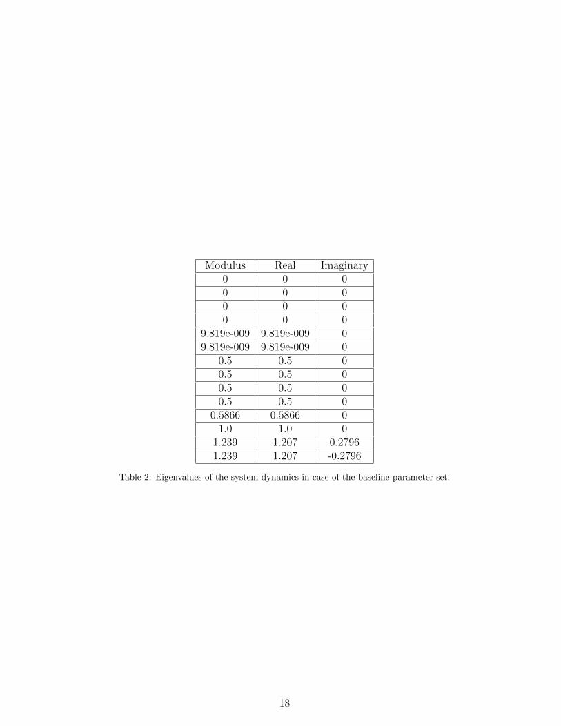
Modulus Real Imaginary0 0 00 0 00 0 00 0 0

9.819e-009 9.819e-009 09.819e-009 9.819e-009 0

0.5 0.5 00.5 0.5 00.5 0.5 00.5 0.5 0

0.5866 0.5866 01.0 1.0 0

1.239 1.207 0.27961.239 1.207 -0.2796

Table 2: Eigenvalues of the system dynamics in case of the baseline parameter set.

18