COUPLING OF TRANSIENTS IN HVDC LINES TO ADJACENT HVAC LINES AND ITS IMPACT ON THE AC LINE PROTECTION Thesis for the Master of Science (MSc) degree Tõnn Arro & Owen Silavwe

Division of Electric Power Engineering Department of Energy & Environment CHALMERS UNIVERSITY OF TECHNOLOGY Göteborg, Sweden 2007

i

COUPLING OF TRANSIENTS IN HVDC LINES TO ADJACENT HVAC LINES AND ITS IMPACT ON THE AC LINE PROTECTION

Tõnn Arro & Owen Silavwe

Division of Electric Power Engineering Department of Energy & Environment

CHALMERS UNIVERSITY OF TECHNOLOGY Göteborg, Sweden, 2007

Department of Energy & Environment Chalmers University of Technology Göteborg, Sweden, 2007 Proposed & Sponsored by: Svenska Kraftnät, Swedish National Grid company Performed at: Chalmers University of Technology Göteborg, Sweden Supervisor: Mr. Kjell-Åke Cederwall Project manager Svenska Kraftnät Examiner: Dr. Daniel Karlsson Division of Electric Power Engineering Department of Energy & Environment Chalmers University of Technology

ii

iii

ACKNOWLEDGEMENTS The authors of this thesis wish to express their special thanks to Mr. Kjell-Åke Cederwall who acted as thesis supervisor from Svenska Kraftnät. Many thanks for affording us an opportunity to perform this thesis work for Svenska Kraftnät and for organizing interesting and educative study visits. The authors also wish to express their gratitude to Dr. Daniel Karlsson, supervisor and examiner for this thesis work at Chalmers University of Technology. His technical insight, advice and patient guidance are gratefully appreciated. Many thanks go to Dr. Tuan A. Le, Prof. Torbjörn Thiringer, Dr. Jörgen Blennow, Dr. Yuriy Serdyuk and Dr. Richard Thomas, all lecturers at Chalmers University, for their support and willingness to help with various aspects of problem solving at very short notice. We are also indebted to Mr. Lidong Zhang at ABB and to Dr. Fainan A. Magueed for their special help in understanding the principles of HVDC control. Our many thanks are extended to Ms. Lillemor Carlshem, Mr. Dag Ingemansson and Mr. Karl-Olof Jonsson, from Svenska Kraftnät, and to Mr. Timo Kiiveri, from Fingrid, who made a special effort in providing us with the necessary system technical information and advice which made it possible for us to perform the coupling studies. The proposition of this thesis and the financial support rendered by Svenska Kraftnät is greatly appreciated, without which this work would not have been possible. Special thanks go to our student colleagues, Björn Karlsson and Pauliina Vottonen, for their information about the availability of this thesis work. Their generosity is greatly appreciated. The authors wish to thank all teachers and fellow students, from Chalmers’ 2006/2007 Electric Power Engineering International Master’s programme, for making this one and half years an interesting and challenging period of study. Finally but not the least, the authors wish to thank their respective families for their special support and love during the period of study at Chalmers University of Technology.

iv

SAMMANFATTNING Föreliggande examensarbete beskriver en studie av kopplingen mellan en högspänd likströmsledning och en högspänd växelströmsledning, som går i samma ledningsgata. Studien har fokuserats på risken för oönskade reläskyddsfunktioner på växelströmsledningen till följd av jordfel på likströmsledningen. Resultaten från den inledande, principiella studien, har sedan applicerats på Fenno-Skan II. Studien visar att jordfel på likströmsledningen inte kommer att leda till oönskad reläskyddsfunktion på någon av de delvis parallella växelströmsledningarna. Den ömsesidiga kopplingen, främst den induktiva, mellan de båda ledningarna, är av sådan storleksordning att den enbart har praktisk betydelse för nollföljdsstorheter. Den ömsesidigt kopplade nollsföljdsströmmens maximala RMS-värden för den totala strömmen respektive fundamentalkomponenten uppgår till 1200A respektive 700A. Dessa strömmar är mycket kortvariga och styrs ned till noll efter 60-80 ms. Jordströmsskydden för de delvis parallella 400kV och 220kV ledningarna kommer, med nuvarande inställningar, inte att lösa ut för dessa kopplade nollföljdsströmmar. Kopplingsstudierna är utförda med modeller som utvecklats i PSCAD/EMTDC och MATLAB. Modellen för PSCAD/EMTDC är detaljerad och representerar hela systemet, medan modellen i MATLAB är enklare och representerar enbart kopplingen mellan ledningarna och är baserad på teorin för stående vågor. En god överensstämmelse mellan resultaten från de båda metoderna har erhållits. Bakgrunden till examensarbetet står att finna i samhällets ökade intresse för miljöfrågor och att hänsyn till vår miljö blir allt viktigare. För att hjälpa till att värna vår miljö är Svenska Kraftnät angelägna om att utnyttja samma ledningsgata för flera ledningar och att sambygga ledningar där det är lämpligt. Detta leder till att ledningar allt oftare går parallellt, med små avstånd mellan ledningarna, vilket leder till starkare ömsesidig koppling mellan ledningarna. Denna koppling kan i sin tur innebära oönskade reläskyddsfunktioner, som påverkar och kanske rentav äventyrar driftsäkerheten. Det är därför viktigt att säkerställa en hög driftsäkerhet och att kontrollera att inga oönskade reläskyddsfunktioner erhålles. Svenska Kraftnät arbetar just nu med en utbyggnad av den befintliga monopolära 400kV, 600MW likströmsförbindelsen mellan Finland och Sverige, Fenno-Skan, till en bipolär ±500kV, 1400MW förbindelse. En del av utbyggnaden planeras som en luftledning i samma ledningsgata som befintliga stamnätsledningar på en sträcka av 70km, från Dannebo till Finnböle. Den nya förbindelsens negativa pol skulle därvid bli parallell med en befintlig 400kV ledning längs en 53km lång sträcka och med en befintlig 220kV ledning längs 7.5km.

v

ABSTRACT With stringent environmental regulations in the world today, acquisition of new rights-of-way (RoW) for transmission projects by electricity companies is at a premium. Faced with this scenario, electricity utilities naturally opt to optimise existing RoW with the consequence that distances between transmission lines in the same RoW are being pushed to the limits. The concern however, for transmission lines located in close proximity with each other is that at non-dc frequency, they will influence each other through electromagnetic coupling. Of interest also is the effect, if any at all, of the resulting coupling on the protection system of the coupled circuit. Svenska Kraftnät (SvK), the Swedish National Grid company, is currently working to expand the existing monopolar 400kV, 600MW Fenno-Skan HVDC link between Sweden and Finland into a bipolar ±500kV, 1400MW link. As one consequence of this expansion, two sections of mutually coupled overhead lines will be created; one coupled section of about 53km will be formed between the second pole (new pole) of the ±500kV HVDC link and an existing 400kV HVAC line and another coupled section between the same pole of the HVDC link with an existing 220kV HVAC line of about 7.5km. The coupled sections arise since the first 70km of the second pole of the HVDC link will be constructed as an overhead line mainly within existing RoWs before transforming into an undersea cable en-route to Finland. In this thesis, the coupling of transients to the HVAC lines that could arise due to a pole-to-ground fault occurring on the HVDC line has been studied in respect of the above mentioned coupled line sections. Furthermore, assessement of the impact of the coupling phenomenon on the ground protection of the HVAC lines has been carried out. The study has been carried out using models developed in PSCAD/EMTDC and MATLAB. The PSCAD/EMTDC model is detailed, taking the form of a full system representation. The MATLAB model is more of a conceptual model, based on solving a system of coupled transmission line travelling wave equations. Good agreement between results from the two models has been achieved. The conclusions of the study are that the coupling phenomenon is mainly due to coupling in zero seuqence networks. Peak values for the RMS coupled zero-sequence currents of 1200A and 700A for total and fundamental currents respectively can be expected. These currents are transient in nature and they decay to zero within about 60-80ms. The study further concludes that the ground overcurrent protection of the coupled 400kV and 220kV AC transmission lines in the SvK system will not be called into operation as a result of the coupled current flowing in them. Finally the study concludes that the ground protection settings in the SvK system can be said to be adequately and properly set such that no unwanted tripping will occur due to this type of coupling phenomenon. Key Words: Coupling Phenomenon, HVDC transmission, HVAC transmission, Right-of-Way (RoW), Zero-Sequence Network, Ground Overcurrent Protection, Ground Protection Settings

vi

TABLE OF CONTENTS ACKNOWLEDGEMENTS............................................................................................... iii SAMMANFATTNING...................................................................................................... iv ABSTRACT........................................................................................................................ v 1. INTRODUCTION .......................................................................................................... 1

1.1. Objective of the Thesis ........................................................................................ 1 1.2. Outline of the Thesis Report ................................................................................ 2

2. THEORETICAL BACKGROUND................................................................................ 4 2.1. HVDC Transmission................................................................................................ 4

2.1.1. Converter Types................................................................................................ 5 2.1.2. CSC Converter .................................................................................................. 6 2.1.3. Ideal Commutation Process .............................................................................. 7 2.1.4. Effect of Valve Firing Control .......................................................................... 9 2.1.5. The Real Commutation Process...................................................................... 10 2.1.6. HVDC Types .................................................................................................. 12

2.2. HVDC Control System .......................................................................................... 15 2.2.1. HVDC Control Basics..................................................................................... 15 2.2.2. Characteristics of HVDC Control System ...................................................... 16 2.2.3. Current Margin Control Method..................................................................... 18 2.2.4. Voltage Dependent Current Limit (VDCL).................................................... 19 2.2.5. Power Flow Reversal ...................................................................................... 19

2.3. HVDC Line Protection .......................................................................................... 20 2.3.1. DC Line Fault Clearing................................................................................... 20 2.3.2. DC-Line Fault Detection Methods.................................................................. 21 2.3.3. Recovery After The Fault ............................................................................... 24

2.4. HVAC Line Protection .......................................................................................... 25 2.4.1. Distance Protection ......................................................................................... 25 2.4.2. Ground Fault Protection.................................................................................. 29

2.5. Mutual Coupling between Lines ............................................................................ 32 2.5.1. Computation of Self & Mutual Inductance/Capacitance ................................ 32 2.5.2. Computation of Coupling Effects ................................................................... 34

3. EXPERIENCES AROUND THE WORLD ................................................................. 39 3.1 HVDC Coupling to HVAC..................................................................................... 39

3.1.1. Coupling Case from Reference [5] ................................................................. 39 3.1.2. Coupling Case from Reference [6] ................................................................. 43 3.1.3. Coupling Case from Reference [7] ................................................................. 44

3.2. HVAC Coupling to HVDC.................................................................................... 45 4. SYSTEM MODEL IN PSCAD .................................................................................... 47

4.1. HVDC System ....................................................................................................... 49 4.1.1. The AC Systems ............................................................................................. 49 4.1.2. Converter Transformers .................................................................................. 49 4.1.3. Converters ....................................................................................................... 50 4.1.4. The DC Side.................................................................................................... 50

vii

4.1.5. AC Filters & Reactive Compensations ........................................................... 51 4.1.6. The Control Systems....................................................................................... 51

4.2. HVAC Lines .......................................................................................................... 54 4.3. AC/DC Line Coupled Sections.............................................................................. 55

5. PSCAD SIMULATION RESULTS ............................................................................. 56 5.1. HVDC System Performance .................................................................................. 56

5.1.1. HVDC Normal Operation ............................................................................... 57 5.1.2. HVDC Operation Under Fault Condition ....................................................... 61

5.2. Coupling Phenomenon – Basecase ........................................................................ 64 5.2.1. Coupled Section 1: RoW Consisting of the HVDC Negative Pole Overhead

Line Section and the 400kV AC Line.............................................................. 67 5.2.2. Coupled Section 2: RoW Consisting of the HVDC Negative Pole Overhead

Line Section and the 220kV AC Line.............................................................. 75 5.3. Sensitivity Analysis ............................................................................................... 81

5.3.1. Effect of Fault Position ................................................................................... 81 5.3.2. Effect of Soil Resistivity................................................................................. 83 5.3.3. Effect of Distance Between Coupled Lines .................................................... 84 5.3.4. Effect of Coupled Section Length................................................................... 85 5.3.5. Effect of Equivalent Terminating Impedance................................................. 87 5.3.6. Effect of fault resistance ................................................................................. 88 5.3.7. Effect of Aerial Ground Wires........................................................................ 89 5.3.8. Effect of AC System Short Circuit Level ....................................................... 90

5.4. Coupling Phenomenon with Monopolar Operation............................................... 92 5.5. Coupling Phenomenon with Reverse Power Operation......................................... 93

6. MATLAB MODEL AND RESULTS .......................................................................... 94 6.1. MATLAB Model ................................................................................................... 94 6.2. Results from the MATLAB Model........................................................................ 95 6.3. Comparison of Results from MATLAB and PSCAD............................................ 96

7. EFFECT OF COUPLED CURRENTS ON THE GROUND PROTECTION OF THE 400KV AC LINES ............................................................................................... 98

8. CONCLUSIONS & RECOMMENDATIONS........................................................... 100 REFERENCES ............................................................................................................... 102 Appendix 1. Geometry of Transmission Lines used in the Study .................................. 104 Appendix 2: Parameters & Impedance Characteristic of the AC Filters at the Rectifier and Inverter End AC systems .................................................................... 106 Appendix 3. MATLAB Program Developed for Calculation of Coupled Currents & Voltages Between Lines in the same RoW................................................ 107

1

1. INTRODUCTION With heightened environmental regulations in the world today coupled with the continuously increasing competition for land among various economic activities, acquisition of new rights-of-way (RoW) for transmission projects by electricity companies is at a premium. Given this scenario, electricity utilities naturally choose to optimise existing RoW with the consequence that distances between transmission lines in the same RoW are being pushed to the limits. The concern however, for transmission lines located in close proximity with each other is that at non-dc frequency, they will influence each other through electromagnetic coupling. Without detailed analysis, it is hardly possible to quantify the amount of coupling that could exist particularly under transient conditions arising due to faults involving ground. Of interest also is the effect, if any at all, of the resulting coupling on the protection system of the coupled circuit.

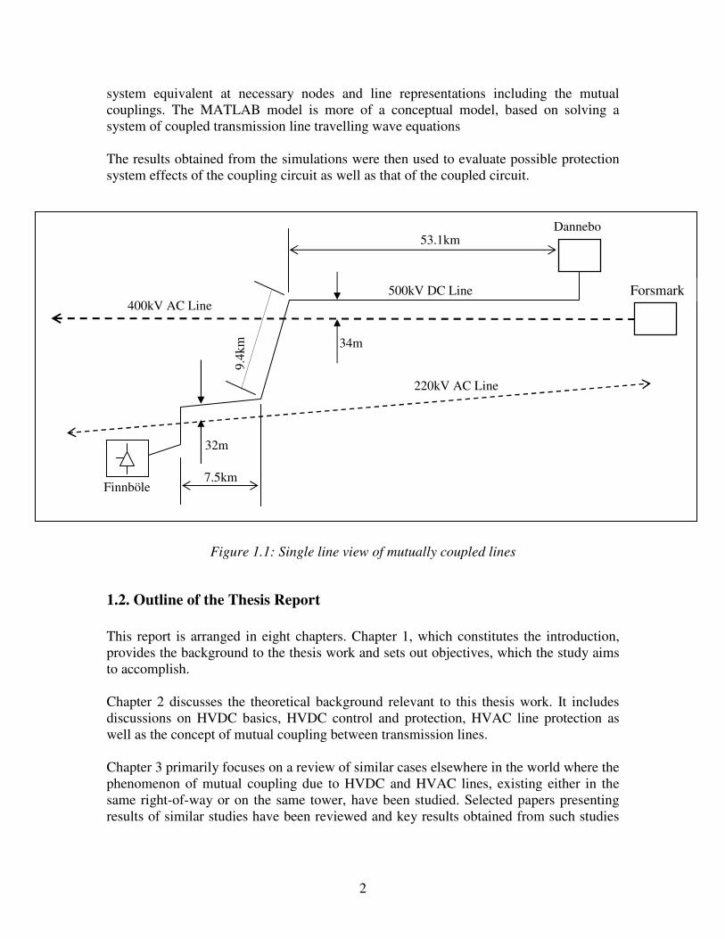
1.1. Objective of the Thesis The main objective of the thesis work presented in this report is to investigate the coupling phenomenon in relation to two corridors of couplings that will be created once Svenska Kraftnät completes the expansion of its currently monopolar 400kV High Voltage Direct Current (HVDC) line between Sweden and Finland into a bipolar arrangement. Svenska Kraftnät (SvK), the Swedish National Transmission company, will soon commence expansion of the 400kV, 600MW monopolar HVDC line between Sweden and Finland into a ±500kV, 1400MW bipolar line. As a consequence of this expansion, two sections of mutually coupled lines will be created; one coupled section of about 53km will be formed between the second pole of the ±500kV HVDC line and an existing 400kV HVAC line and another coupled section between the same pole of the HVDC line with an existing 220kV HVAC line of about 7.5km. This situation is shown pictorially in Figure 1.1 below. The coupled sections arise since the first 70km of the second pole of the HVDC line will be constructed as an overhead line mainly within existing RoWs before transforming into an undersea cable on its route to Finland. This study focuses on the coupling of transients in the HVDC line to the HVAC lines within the same right of way arising as a result of a line-to-ground (LG) fault occurring on the HVDC line. The study further assesses what impact this phenomenon has on the protection of the HVAC lines and whether the HVDC protection and control can play any role in this phenomenon. To study this phenomenon, system models were developed in PSCAD/EMTDC and MATLAB. The PSCAD/EMTDC model is quite detailed, taking the form of a full system representation that includes the HVDC system together with its controls, the power

2

system equivalent at necessary nodes and line representations including the mutual couplings. The MATLAB model is more of a conceptual model, based on solving a system of coupled transmission line travelling wave equations The results obtained from the simulations were then used to evaluate possible protection system effects of the coupling circuit as well as that of the coupled circuit.

Figure 1.1: Single line view of mutually coupled lines

1.2. Outline of the Thesis Report This report is arranged in eight chapters. Chapter 1, which constitutes the introduction, provides the background to the thesis work and sets out objectives, which the study aims to accomplish. Chapter 2 discusses the theoretical background relevant to this thesis work. It includes discussions on HVDC basics, HVDC control and protection, HVAC line protection as well as the concept of mutual coupling between transmission lines. Chapter 3 primarily focuses on a review of similar cases elsewhere in the world where the phenomenon of mutual coupling due to HVDC and HVAC lines, existing either in the same right-of-way or on the same tower, have been studied. Selected papers presenting results of similar studies have been reviewed and key results obtained from such studies

9.4k

m

53.1km

7.5km

32m

34m

500kV DC Line

Finnböle

Dannebo

220kV AC Line

400kV AC Line Forsmark

3

by different authors are presented in this chapter. Furthermore, a brief section on the coupling of HVAC to HVDC is also included in this chapter. This is followed by chapter 4, which is dedicated to the description of system modelling carried out in PSCAD. In Chapter 5 a discussion and analysis of results from PSCAD simulations is presented. This chapter is then followed by Chapter 6, where a coupling model for two lines in the same RoW, built in MATLAB, is presented. Chapter 7 then focuses on the discussion of effects of the coupled currents on the ground protection of the AC lines. Finally chapter 8, aimed at detailing overall conclusions of the thesis work, forms the last chapter of the report.

4

2. THEORETICAL BACKGROUND This chapter gives the theoretical background necessary for the study of the coupling phenomena that may occur between transmission lines. The first part of the chapter is divided into three parts – HVDC transmission, HVDC control and DC line protection. The transmission part considers the basics of HVDC conversion, the rectifier and inverter operations of HVDC converters, the commutation process in the converters and describes the main configurations of two-terminal HVDC systems. The control part discusses the basics of HVDC control and the main functions and characteristics of the rectifier and inverter control systems. The HVDC line protection part describes how the DC line fault is detected and cleared by the protection system and how normal operation is resumed after the fault. Different methods of DC line fault detection are also considered. The second part of this chapter covers the HVAC line protection methods that are relevant to this thesis work, more specifically the distance protection and ground fault protection. The third part covers the mutual coupling phenomena between two transmission lines. Firstly, a description of the coupling effects between two transmission lines is given. This is followed by the calculation method of self and mutual inductances and capacitances. Finally, a computation method of coupling effects between two transmission lines is given in this chapter. 2.1. HVDC Transmission There are lots of advantages that favour DC transmission over AC. First, the cost of AC and DC transmission has to be compared. When comparing AC and DC lines of the same voltage level, a DC line can carry as much power with two conductors as an AC line with three conductors of the same size. Therefore the right-of-way (ROW) required for the transmission line of a given power level is significantly smaller for a DC line. Other benefits for DC line are simpler and cheaper towers, reduced conductor and insulation costs [1]. From the point of view of power losses, DC losses are around two-thirds of the comparable AC system losses, since there are only two conductors [1]. All the factors together result in significant savings of the DC transmission line as compared to the equivalent AC line. A drawback of DC transmission is the high cost of converter stations, which counteracts the economical gain of the DC transmission line. DC transmission becomes economically justified only after exceeding the breakeven distance between two converter stations. For

5

overhead lines this is between 400 to 700 km and for cables between 25 to 50 km [1]. When the breakeven distance is exceeded, the total cost of DC transmission becomes cheaper than AC. From a technical point of view there are many positive characteristics of DC transmission. One point is that the DC line itself does not require any reactive power compensation, but on the other hand, the converter stations consume a lot of reactive power, which can be up to 60% of the station’s power rating. An advantage of DC transmission is also the possibility to use a DC link in order to improve the stability of an AC system, because the power flow in a DC system can easily be controlled at high speed. Moreover, the power carrying capability of a DC link is unaffected by the transmission distance, which is not true for AC, where it is inversely proportional to the distance. The transmission distance with AC cables is limited up to 50km due to the high steady-state charging currents. This restriction does not exist for DC cables, thus making the breakeven distance up to 50 km. Final benefits are that DC links can be used to connect two AC systems with different frequencies or different control philosophies. When two AC networks are interconnected by a DC link, the fault level of the system does not increase significantly, which is not the case with AC connections [3]. The biggest drawbacks of DC transmission are [1]:

1. High cost of converter stations, 2. Transformers cannot be used to alter voltage levels, 3. Harmonics generated by the converter stations need to be filtered out, 4. Requirement of reactive power by the converter stations and 5. Complex controls of DC transmission.

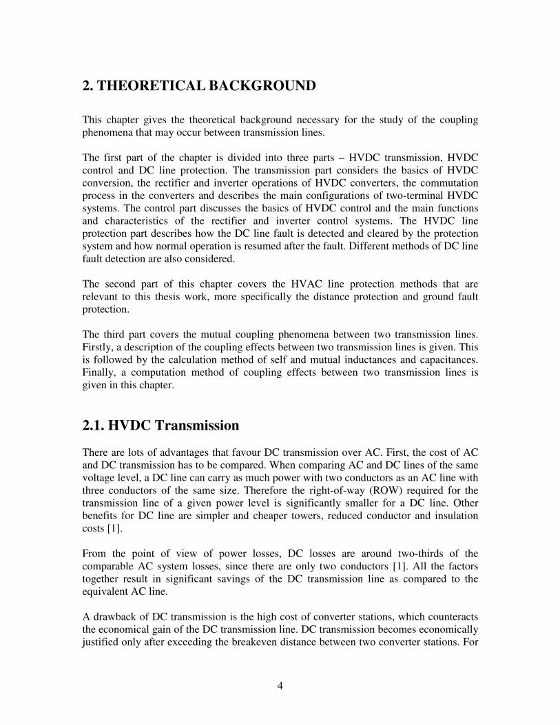
2.1.1. Converter Types A converter is required in the HVDC system for converting electrical energy from AC to DC or vice-versa. Two main three-phase converter types exist in the world today (Figure 2.1) [1]:

• Current source converter (CSC) and • Voltage source converter (VSC).

6

Figure 2.1: (a) CSC and (b) VSC

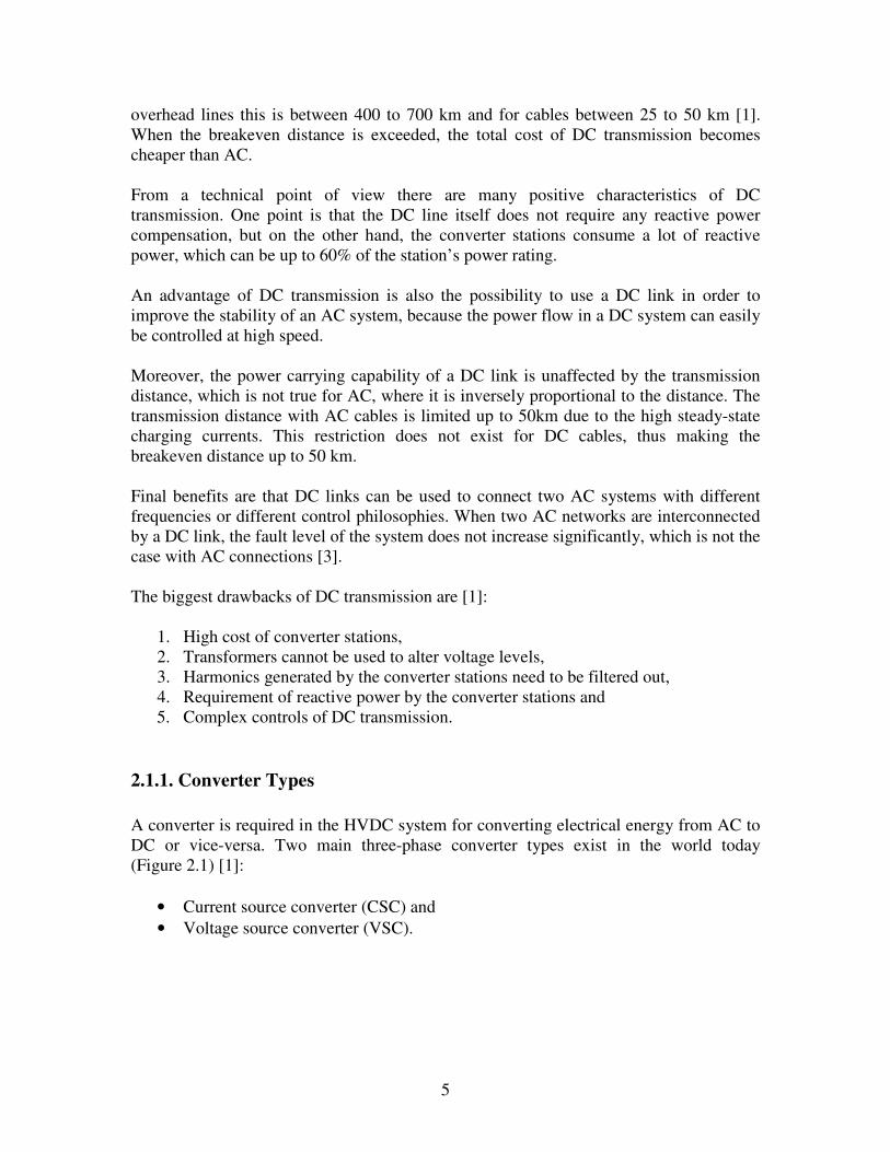
Up to 1990s, CSC configuration has been used almost exclusively. Mercury arc valves have been implemented in the CSCs as the fundamental switching devices up to 1970s, when they were replaced by thyristor valves [1]. Since 1990s, VSC type of converters have also been available for use in HVDC systems. The choice of which converter type to choose for a particular project is based upon economic and technical considerations of the system. Currently, the main obstacle for wider use of VSC type is its limited power range up to a couple of hundred MW [1]. A comparison between the characteristics of the two converters is given in table 2.1 [1]: Table 2.1: Comparison between converter types

Converter type CSC VSC

On AC side Acts as a constant voltage source Capacitor required for energy storage Large AC filters required for harmonic elimination Reactive power supply necessary for power factor correction

Acts as a constant current source Inductor needed for energy storage Only a small AC filter needed for higher harmonics elimination No reactive power supply needed since the converter can operate in any quadrant

On DC side Acts as a constant current source Inductor needed for energy storage DC filters required Provides inherent fault current limiting features

Acts as a constant voltage source Capacitor needed for energy storage This capacitor provides DC filtering Problems with DC line faults since the capacitor discharges into the fault

Switches Line commutated or force commutated with a series capacitor Switching at line frequency (single pulsing per cycle) Lower switching losses

Self-commutated Switching at high frequency (multiple pulsing in one cycle) Higher switching losses

2.1.2. CSC Converter The main converter type used for higher power HVDC transmission is the CSC. It is also the system used in the Fenno-Skan HVDC project and therefore a description of its operation is provided next.

7

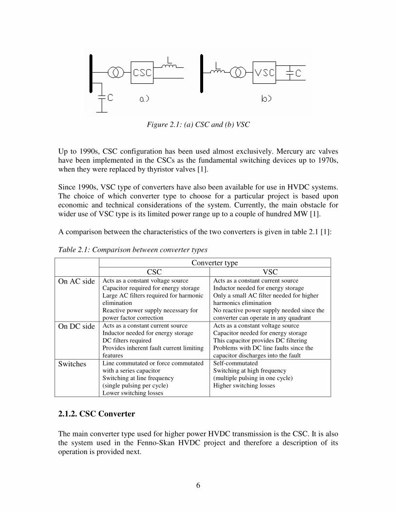
CSC utilizes thyristor valves as switching devices, which are connected in a three-phase bridge configuration (Figure 2.2) for both, rectifier and inverter operations. A valve is a combination of thyristors that are arranged in series and in parallel to meet the required current and voltage ratings. Va, Vb and Vc in Figure 2.2 denote 3-phase voltages of the AC system and Xc is the commutation reactance of each phase. Vd is the output DC voltage. The bridge configuration is used due to the lower peak-inverse voltage across the converter valves and better utilisation of the converter transformer when compared to other possible alternatives like three-phase double star or six-phase diametrical connections [3].

Figure 2.2: Three-phase, 6-pulse thyristor valve bridge

From Figure 2.2 it can be seen that two valves are connected to each phase terminal, upper one with the anode connected to it and lower one with the cathode connected to it. Thyristor valves turn on and conduct current when they receive a firing pulse from the control system and are forward biased (voltage across the valve is positive). They conduct current until the valves become reverse biased (negative voltage across the valve) and current reaches zero. The valves are fired in successive order, which is indicated by the numbers in Figure 2.2, so that the current would commutate from one valve pair to another as smoothly as possible [4].

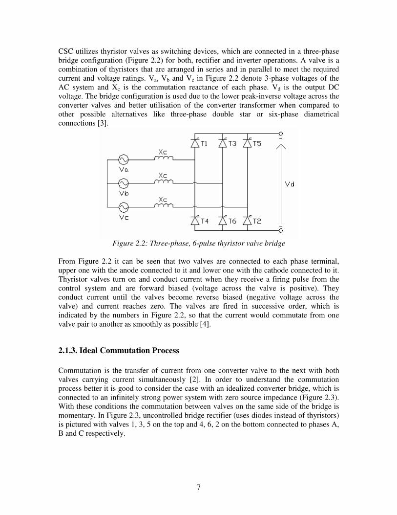
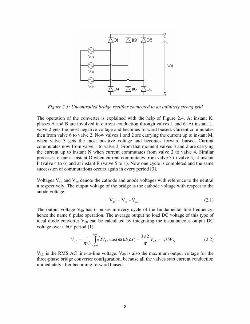
2.1.3. Ideal Commutation Process Commutation is the transfer of current from one converter valve to the next with both valves carrying current simultaneously [2]. In order to understand the commutation process better it is good to consider the case with an idealized converter bridge, which is connected to an infinitely strong power system with zero source impedance (Figure 2.3). With these conditions the commutation between valves on the same side of the bridge is momentary. In Figure 2.3, uncontrolled bridge rectifier (uses diodes instead of thyristors) is pictured with valves 1, 3, 5 on the top and 4, 6, 2 on the bottom connected to phases A, B and C respectively.

8

Figure 2.3: Uncontrolled bridge rectifier connected to an infinitely strong grid

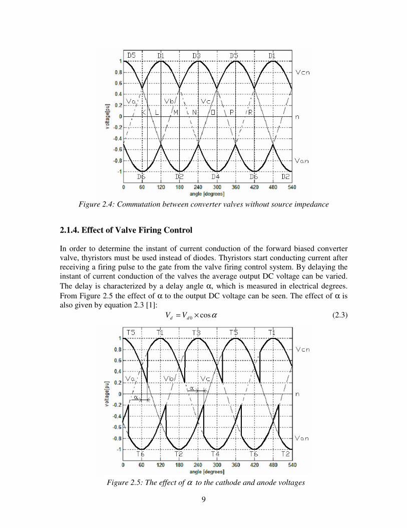
The operation of the converter is explained with the help of Figure 2.4. At instant K, phases A and B are involved in current conduction through valves 1 and 6. At instant L, valve 2 gets the most negative voltage and becomes forward biased. Current commutates then from valve 6 to valve 2. Now valves 1 and 2 are carrying the current up to instant M, when valve 3 gets the most positive voltage and becomes forward biased. Current commutates now from valve 1 to valve 3. From that moment valves 3 and 2 are carrying the current up to instant N when current commutates from valve 2 to valve 4. Similar processes occur at instant O when current commutates from valve 3 to valve 5, at instant P (valve 4 to 6) and at instant R (valve 5 to 1). Now one cycle is completed and the same succession of commutations occurs again in every period [3]. Voltages Vcn and Van denote the cathode and anode voltages with reference to the neutral n respectively. The output voltage of the bridge is the cathode voltage with respect to the anode voltage:

ancnd0 V-VV = (2.1)

The output voltage Vd0 has 6 pulses in every cycle of the fundamental line frequency, hence the name 6 pulse operation. The average output no load DC voltage of this type of ideal diode converter Vd0 can be calculated by integrating the instantaneous output DC voltage over a 60° period [1]:

LLLLLLd VVtdtVV 35,123

)()cos(23

1 6

60 ===

− πωω

π

π

π

(2.2)

VLL is the RMS AC line-to-line voltage. Vd0 is also the maximum output voltage for the three-phase bridge converter configuration, because all the valves start current conduction immediately after becoming forward biased.

9

Figure 2.4: Commutation between converter valves without source impedance

2.1.4. Effect of Valve Firing Control In order to determine the instant of current conduction of the forward biased converter valve, thyristors must be used instead of diodes. Thyristors start conducting current after receiving a firing pulse to the gate from the valve firing control system. By delaying the instant of current conduction of the valves the average output DC voltage can be varied. The delay is characterized by a delay angle α, which is measured in electrical degrees. From Figure 2.5 the effect of α to the output DC voltage can be seen. The effect of α is also given by equation 2.3 [1]:

αcos0 ×= dd VV (2.3)

Figure 2.5: The effect of α to the cathode and anode voltages

10

With a large smoothing reactor on the DC side, the voltage waveform in Figure 2.5 produces a constant direct current whose magnitude is dependant on the average DC voltages at both ends of the DC link and on the link resistance [3]. The higher the delay angle α is, the lower the average output voltage Vd becomes. With diode operation (α = 0) the output voltage Vd0 is the highest and it is reduced in proportion to the increase of α. When α = 90°, the average output DC voltage is 0. When α exceeds 90°, the mean DC output voltage Vd becomes negative and the bridge operation can only be sustained with a DC power supply. Due to the supply, the current flows in the same direction through the converter valves (from anode to cathode) in opposition to the induced e.m.f in the converter transformer. This way, power is being fed to the AC system from the DC system, i.e. the converter acts as an inverter. There are 3 conditions necessary for inverter operation [3]:

1) three-phase AC voltage must be provided by the AC system 2) converter firing angle α must be higher than 90° 3) presence of a DC power supply.

Maximum power inversion in ideal case would occur with a delay angle of 180°, but in reality this is not feasible, because no time would be left for current commutation.

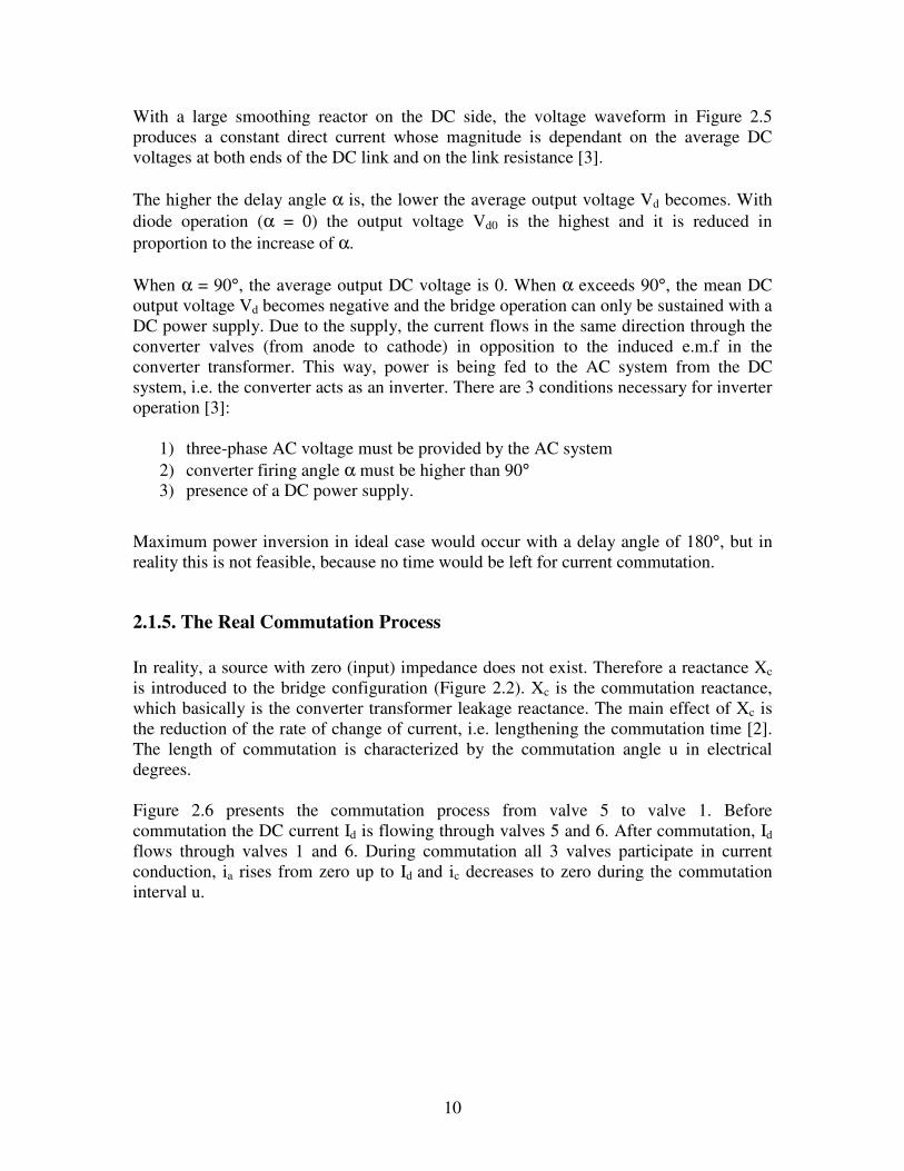
2.1.5. The Real Commutation Process In reality, a source with zero (input) impedance does not exist. Therefore a reactance Xc is introduced to the bridge configuration (Figure 2.2). Xc is the commutation reactance, which basically is the converter transformer leakage reactance. The main effect of Xc is the reduction of the rate of change of current, i.e. lengthening the commutation time [2]. The length of commutation is characterized by the commutation angle u in electrical degrees. Figure 2.6 presents the commutation process from valve 5 to valve 1. Before commutation the DC current Id is flowing through valves 5 and 6. After commutation, Id flows through valves 1 and 6. During commutation all 3 valves participate in current conduction, ia rises from zero up to Id and ic decreases to zero during the commutation interval u.

11

Figure 2.6: (a) Equivalent circuit of the commutation from valve 5 to valve 1 (b) The commutation currents During commutation, commutation current iu flows from the conducting valve 5 to valve 1 and is equal to phase a current ia:

iu ia = (2.4)

Voltage drop V occurs on inductance Xc during commutation:

)()(

tddi

Xdtdi

XV uc

uc ω

ω ==∆ (2.5)

During the commutation interval u, current iu rises from 0 to Id. When integrating equation 2.5 over the commutation period, voltage drop V can be found:

udc

I

uc

u

AIXdiXtdVd

===∆ 00

)(ω (2.6)

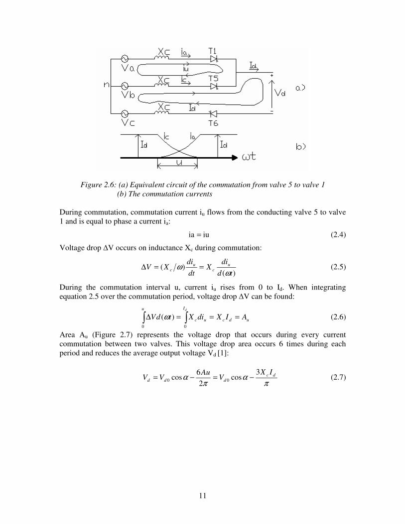
Area Au (Figure 2.7) represents the voltage drop that occurs during every current commutation between two valves. This voltage drop area occurs 6 times during each period and reduces the average output voltage Vd [1]:

π

απ

α dcddd

IXV

AuVV

3cos

26

cos 00 −=−= (2.7)

12

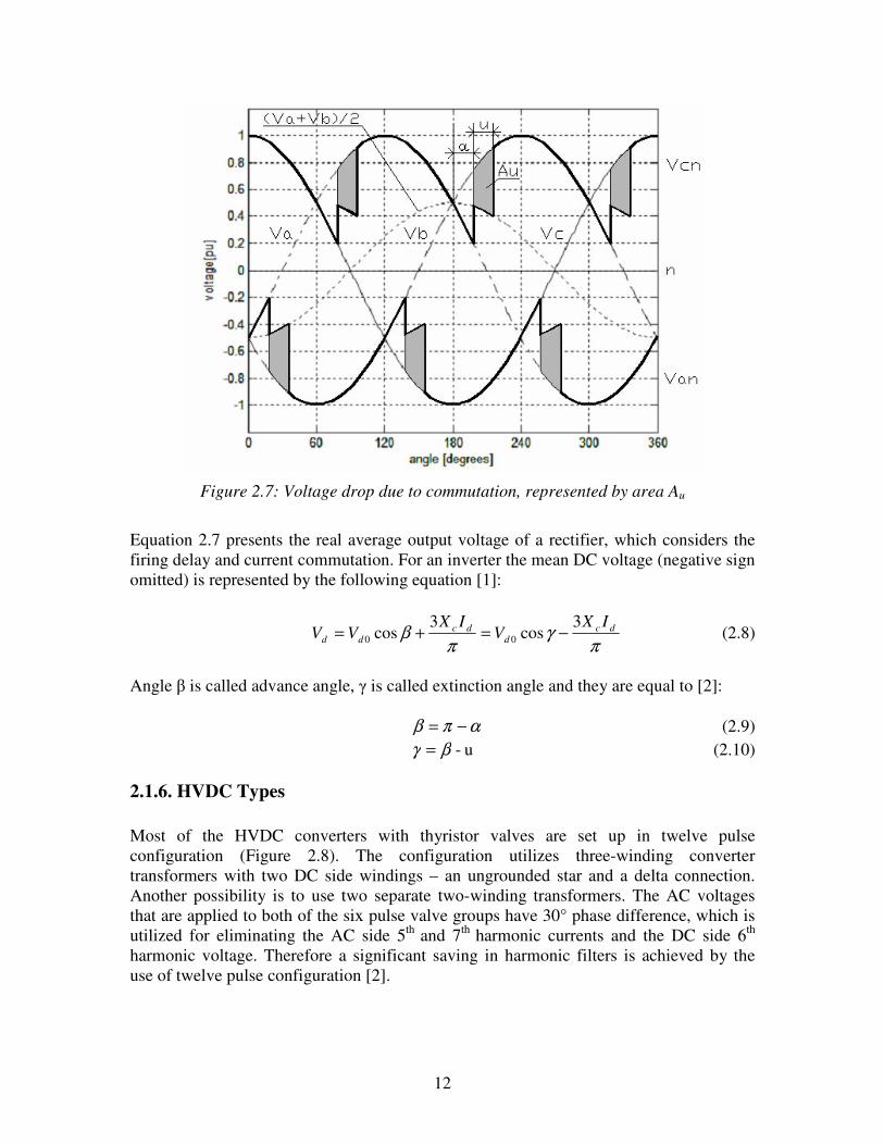
Figure 2.7: Voltage drop due to commutation, represented by area Au

Equation 2.7 presents the real average output voltage of a rectifier, which considers the firing delay and current commutation. For an inverter the mean DC voltage (negative sign omitted) is represented by the following equation [1]:

π

γπ

β dcd

dcdd

IXV

IXVV

3cos

3cos 00 −=+= (2.8)

Angle is called advance angle, is called extinction angle and they are equal to [2]:

απβ −= (2.9) u-βγ = (2.10)

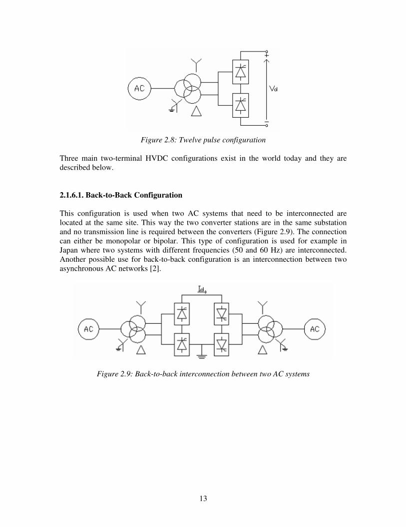
2.1.6. HVDC Types Most of the HVDC converters with thyristor valves are set up in twelve pulse configuration (Figure 2.8). The configuration utilizes three-winding converter transformers with two DC side windings – an ungrounded star and a delta connection. Another possibility is to use two separate two-winding transformers. The AC voltages that are applied to both of the six pulse valve groups have 30° phase difference, which is utilized for eliminating the AC side 5th

and 7th harmonic currents and the DC side 6th

harmonic voltage. Therefore a significant saving in harmonic filters is achieved by the use of twelve pulse configuration [2].

13

Figure 2.8: Twelve pulse configuration

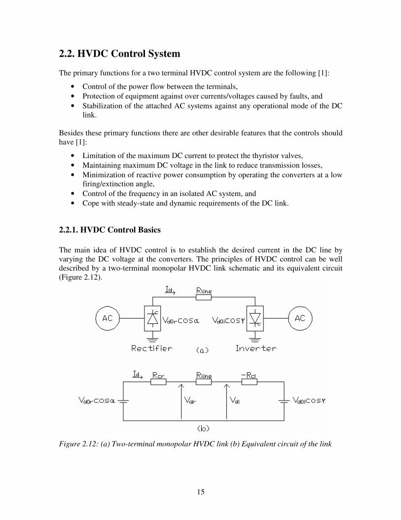
Three main two-terminal HVDC configurations exist in the world today and they are described below. 2.1.6.1. Back-to-Back Configuration This configuration is used when two AC systems that need to be interconnected are located at the same site. This way the two converter stations are in the same substation and no transmission line is required between the converters (Figure 2.9). The connection can either be monopolar or bipolar. This type of configuration is used for example in Japan where two systems with different frequencies (50 and 60 Hz) are interconnected. Another possible use for back-to-back configuration is an interconnection between two asynchronous AC networks [2].

Figure 2.9: Back-to-back interconnection between two AC systems

14

2.1.6.2. Monopolar Configuration Two converter stations that are separated from each other are connected by a single conductor and earth (or sea) is used as a return conductor (Figure 2.10). If the use of earth for current return is prohibited a metallic return conductor can be used instead [2].

Figure 2.10: Monopolar HVDC connection

2.1.6.3. Bipolar Configuration A bipolar HVDC configuration consists of two combined monopolar HVDC systems, one at positive and one at negative polarity with respect to ground. Both of the monopolar systems can operate separately with ground return when one pole is out of service, resulting in higher reliability of the overall system. By appropriate switching, one DC line can also be used as a return conductor during faulty conditions. But when both poles carry equal current, the total ground current is zero. Ground is only used for current conduction in the case of an emergency or when one pole is not operating [2].

A bipolar configuration is also going to be implemented in the Fenno-Skan project .

Figure 2.11: Bipolar HVDC connection

15

2.2. HVDC Control System The primary functions for a two terminal HVDC control system are the following [1]:

• Control of the power flow between the terminals, • Protection of equipment against over currents/voltages caused by faults, and • Stabilization of the attached AC systems against any operational mode of the DC

link.

Besides these primary functions there are other desirable features that the controls should have [1]:

• Limitation of the maximum DC current to protect the thyristor valves, • Maintaining maximum DC voltage in the link to reduce transmission losses, • Minimization of reactive power consumption by operating the converters at a low

firing/extinction angle, • Control of the frequency in an isolated AC system, and • Cope with steady-state and dynamic requirements of the DC link.

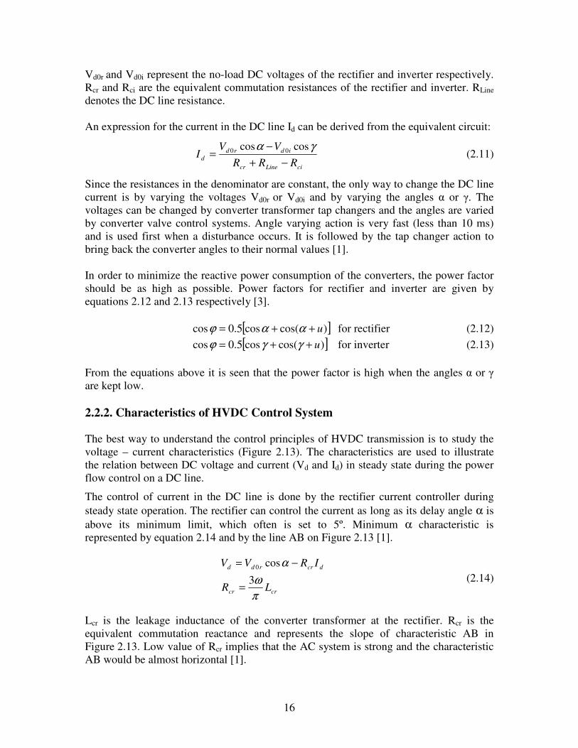
2.2.1. HVDC Control Basics The main idea of HVDC control is to establish the desired current in the DC line by varying the DC voltage at the converters. The principles of HVDC control can be well described by a two-terminal monopolar HVDC link schematic and its equivalent circuit (Figure 2.12).

Figure 2.12: (a) Two-terminal monopolar HVDC link (b) Equivalent circuit of the link

16

Vd0r and Vd0i represent the no-load DC voltages of the rectifier and inverter respectively. Rcr and Rci are the equivalent commutation resistances of the rectifier and inverter. RLine denotes the DC line resistance. An expression for the current in the DC line Id can be derived from the equivalent circuit:

ciLinecr

idrdd RRR

VVI

−+−

=γα coscos 00 (2.11)

Since the resistances in the denominator are constant, the only way to change the DC line current is by varying the voltages Vd0r or Vd0i and by varying the angles or . The voltages can be changed by converter transformer tap changers and the angles are varied by converter valve control systems. Angle varying action is very fast (less than 10 ms) and is used first when a disturbance occurs. It is followed by the tap changer action to bring back the converter angles to their normal values [1]. In order to minimize the reactive power consumption of the converters, the power factor should be as high as possible. Power factors for rectifier and inverter are given by equations 2.12 and 2.13 respectively [3].

[ ])cos(cos5.0cos u++= ααϕ for rectifier (2.12) [ ])cos(cos5.0cos u++= γγϕ for inverter (2.13)

From the equations above it is seen that the power factor is high when the angles or are kept low. 2.2.2. Characteristics of HVDC Control System The best way to understand the control principles of HVDC transmission is to study the voltage – current characteristics (Figure 2.13). The characteristics are used to illustrate the relation between DC voltage and current (Vd and Id) in steady state during the power flow control on a DC line.

The control of current in the DC line is done by the rectifier current controller during steady state operation. The rectifier can control the current as long as its delay angle α is above its minimum limit, which often is set to 5º. Minimum α characteristic is represented by equation 2.14 and by the line AB on Figure 2.13 [1].

crcr

dcrrdd

LR

IRVV

πω

α3

cos0

=

−= (2.14)

Lcr is the leakage inductance of the converter transformer at the rectifier. Rcr is the equivalent commutation reactance and represents the slope of characteristic AB in Figure 2.13. Low value of Rcr implies that the AC system is strong and the characteristic AB would be almost horizontal [1].

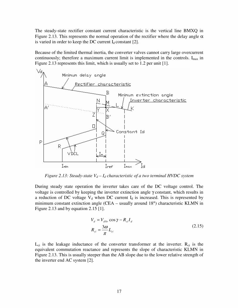
17

The steady-state rectifier constant current characteristic is the vertical line BMXQ in Figure 2.13. This represents the normal operation of the rectifier where the delay angle α is varied in order to keep the DC current Id constant [2]. Because of the limited thermal inertia, the converter valves cannot carry large overcurrent continuously; therefore a maximum current limit is implemented in the controls. Imax in Figure 2.13 represents this limit, which is usually set to 1.2 per unit [1].

Figure 2.13: Steady-state Vd – Id characteristic of a two terminal HVDC system During steady state operation the inverter takes care of the DC voltage control. The voltage is controlled by keeping the inverter extinction angle γ constant, which results in a reduction of DC voltage Vd when DC current Id is increased. This is represented by minimum constant extinction angle (CEA – usually around 18°) characteristic KLMN in Figure 2.13 and by equation 2.15 [1].

cici

dcirdd

LR

IRVV

πω

γ3

cos0

=

−= (2.15)

Lci is the leakage inductance of the converter transformer at the inverter. Rci is the equivalent commutation reactance and represents the slope of characteristic KLMN in Figure 2.13. This is usually steeper than the AB slope due to the lower relative strength of the inverter end AC system [2].

18

Another possible operating mode for the inverter is constant voltage operation, which is represented by line LXY in Figure 2.13. For operation according to this characteristic, the inverter extinction angle γ must be increased beyond its minimum level [2]. The operating point of the HVDC system is represented by the intersection of the rectifier and inverter characteristics. In this case it is point X for inverter constant Vd control or point M for inverter constant control [2]. The operating point is achieved with the help of the converter transformer on-line tap changers. For rectifier the transformer on-line tap changer is used to keep the delay angle α at its normal operating range to meet the constant current setting Iref. For inverter operation, the on-line tap changer adjusts accordingly to meet the desired level of DC voltage (for minimum constant control) or extinction angle (constant Vd control) [2]. When the inverter is operating at point X and the DC current order at the rectifier Iref is increased beyond point L, the inverter changes its control philosophy from constant Vd to constant control and operates according to the line KL. DC voltage becomes lower than the desired level and the inverter transformer on-line tap changer has to increase its DC side voltage to turn back to constant voltage control [2]. The constant DC voltage characteristic (line LXY in Figure 2.13) is not used in all HVDC control systems. Voltage control can be achieved also with the cooperation of constant extinction angle characteristic (line KLMN) and transformer on-line tap changer [2].

2.2.3. Current Margin Control Method When the rectifier is operating at a higher delay angle than minimum (5º), it is controlling the current in the DC line. But the inverter also has a current controller that is characterized by the section NYO in Figure 2.13. Both current controllers receive the current order Iref. The rectifier current controller tries to maintain that current in the DC line, but the inverter current controller tries to keep the DC line current at a slightly lower value. The difference between the currents is the current margin Im, which is usually 0.1 per unit. In normal steady state operation, the inverter current controller is forced out of action and the rectifier keeps the current reference in the DC line. The inverter current controller is active only when the rectifier is operating with minimum delay angle α and keeps the current in the DC line at a value Iref – Im [2]. The minimum α characteristic is line AB on Figure 2.13. If the rectifier voltage should fall below points N or Y (line A’B’), due to an AC voltage drop for example, the operating point of the HVDC system changes. A new operating point is formed at the intersection of the A’B’ characteristic and the inverter constant current characteristic NYO and is denoted by Z. The Inverter has now taken over the current control, keeping the DC current at Iref – Im and the rectifier is controlling the DC voltage as long as it operates at its minimum α characteristic [2].

19

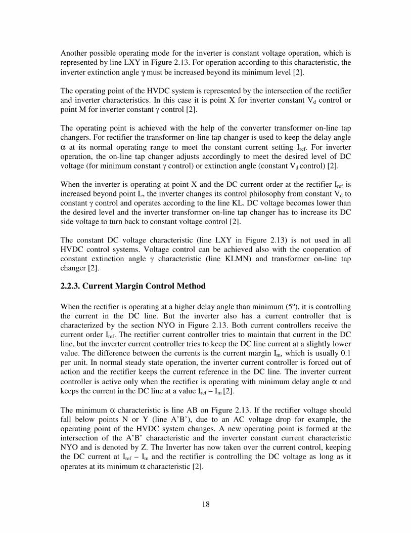
2.2.4. Voltage Dependent Current Limit (VDCL) Lines QR and OP on Figure 2.13 denote the rectifier and inverter voltage dependent current limit (VDCL) characteristics. These characteristics reduce the DC current order if the DC voltage decreases, e.g. due to an AC system disturbance. In order to maintain the operation of the AC system, VDCL limits the current in the DC line. When normal operation has returned and the DC voltage recovered, current returns to its steady-state level Iref [2]. The rectifier VDCL characteristic is usually terminated with a minimum DC current limit Imin, which is usually set between 0.2 to 0.3 per unit. The Imin limit is implemented for keeping enough DC current in the valves to avoid reaching discontinuous current operation, which might result in dangerous, transient overvoltages [1].

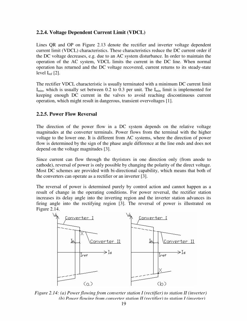
2.2.5. Power Flow Reversal The direction of the power flow in a DC system depends on the relative voltage magnitudes at the converter terminals. Power flows from the terminal with the higher voltage to the lower one. It is different from AC systems, where the direction of power flow is determined by the sign of the phase angle difference at the line ends and does not depend on the voltage magnitudes [3].

Since current can flow through the thyristors in one direction only (from anode to cathode), reversal of power is only possible by changing the polarity of the direct voltage. Most DC schemes are provided with bi-directional capability, which means that both of the converters can operate as a rectifier or an inverter [3].

The reversal of power is determined purely by control action and cannot happen as a result of change in the operating conditions. For power reversal, the rectifier station increases its delay angle into the inverting region and the inverter station advances its firing angle into the rectifying region [3]. The reversal of power is illustrated on Figure 2.14.

Figure 2.14: (a) Power flowing from converter station I (rectifier) to station II (inverter) (b) Power flowing from converter station II (rectifier) to station I (inverter)

20

2.3. HVDC Line Protection The general philosophy of HVDC protection is similar to that of the AC and its main desired features can be summarized as follows [11]:

1. All abnormal conditions that expose hazard to the protected equipment or cause an unacceptable operating condition must be detected and cleared by the protective system.

2. All protections must be fully redundant and based on different operating principles if possible.

3. Selectivity – only the minimum system around the fault should be separated.

4. False tripping of sound equipment must be avoided.

5. Protective systems must have separate communication channels to the AC breakers and to the converter valves – communication paths should be redundant.

6. Backup protection must be provided in the case of failure of the primary protection.

7. DC protection systems must be coordinated with nearby AC protections to ensure the best performance of both systems.

8. Testing of the protective systems should be possible without affecting the operation of the HVDC system.

HVDC protection is a complex system with a hierarchical structure where all equipment is protected by various measures and principles. It is sometimes difficult to clearly distinguish between a protective and a control function as they are performed by the same or similar devices [11]. Since the scope of this thesis is DC-line-to-ground fault, only DC-line protection is considered in the following chapters.

2.3.1. DC Line Fault Clearing DC line short circuit is different from AC short circuit, because once DC fault starts it will not be extinguished by itself until the current is reduced to zero and the arc is deionised. Nevertheless, most DC line faults are caused by lightning and are, similarly to AC faults, self-clearing, because the arc is deionised at the current zeroes due to line oscillations, but this cannot be guaranteed. Thus, there has to be some control function that brings the current down to zero when a fault occurs on a DC line. The amplitude of the DC line fault current is smaller than the AC one; usually limited to two or three per unit by the smoothing reactor and by control action [3]. The objective of the DC-line protection is to detect ground faults on the DC-line and extinguish the fault current by control action. In case the fault is not permanent, pre-fault

21

power transmission should be restored by control action after sufficient time delay for arc deionisation [11]. After the fault detection, the rectifier is forced to full inversion operation and does not supply any current to the fault [11]. This is done by increasing the firing angle over 90º into inverting region and it is kept at that value until the arc extinction and deionisation is likely to be completed [3]. The inverter voltage already has the correct polarity, thus the two converters are temporarily inverting at the same time and transferring the energy stored in the DC circuit electric and magnetic fields into the two AC systems. The inverter firing delay is advanced at the same time, but a limitation is set to 90º to prevent the inverter from going into the rectifying region. By this control action the fault arc can be deionised and the fault cleared very rapidly when compared with AC protection [3].

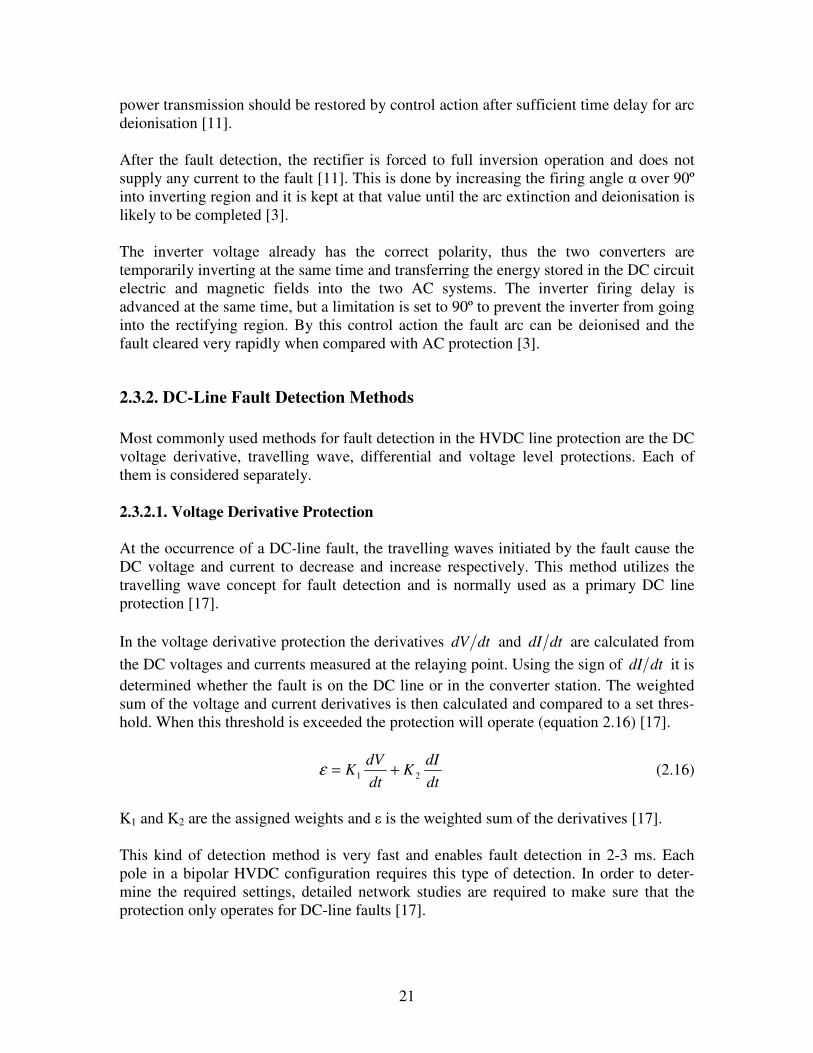
2.3.2. DC-Line Fault Detection Methods Most commonly used methods for fault detection in the HVDC line protection are the DC voltage derivative, travelling wave, differential and voltage level protections. Each of them is considered separately. 2.3.2.1. Voltage Derivative Protection At the occurrence of a DC-line fault, the travelling waves initiated by the fault cause the DC voltage and current to decrease and increase respectively. This method utilizes the travelling wave concept for fault detection and is normally used as a primary DC line protection [17]. In the voltage derivative protection the derivatives dtdV and dtdI are calculated from the DC voltages and currents measured at the relaying point. Using the sign of dtdI it is determined whether the fault is on the DC line or in the converter station. The weighted sum of the voltage and current derivatives is then calculated and compared to a set thres-hold. When this threshold is exceeded the protection will operate (equation 2.16) [17].

dtdI

KdtdV

K 21 +=ε (2.16)

K1 and K2 are the assigned weights and is the weighted sum of the derivatives [17]. This kind of detection method is very fast and enables fault detection in 2-3 ms. Each pole in a bipolar HVDC configuration requires this type of detection. In order to deter-mine the required settings, detailed network studies are required to make sure that the protection only operates for DC-line faults [17].

22

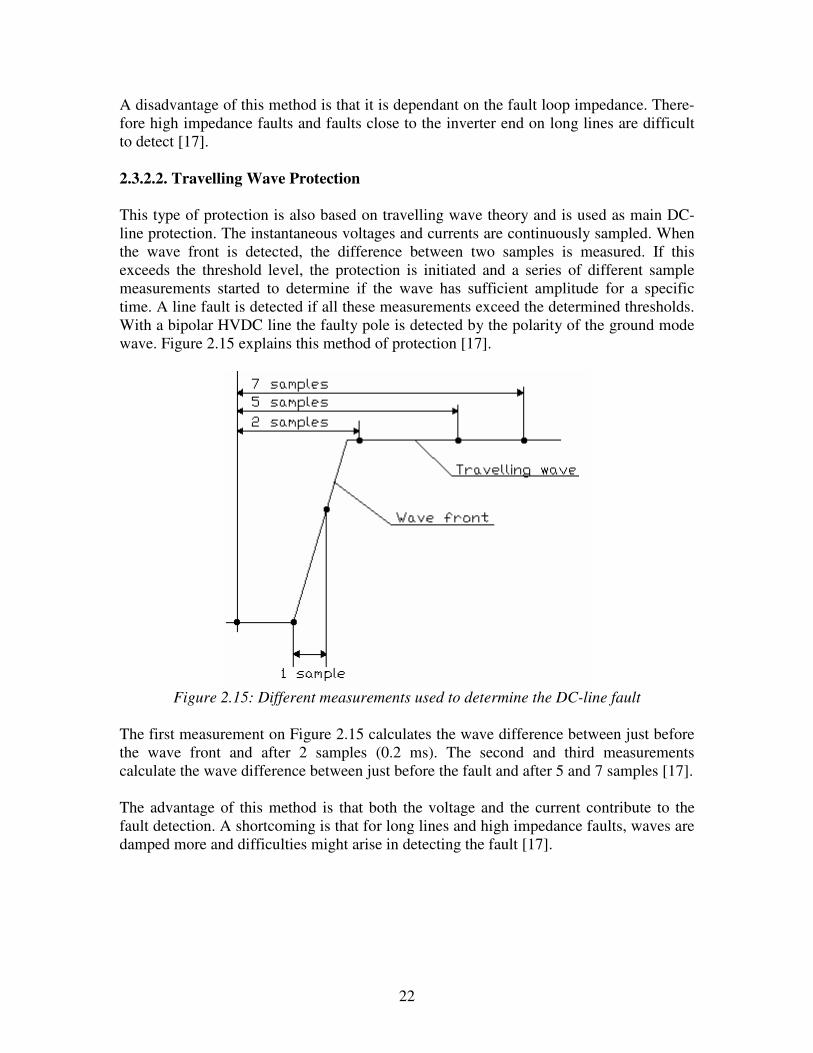
A disadvantage of this method is that it is dependant on the fault loop impedance. There-fore high impedance faults and faults close to the inverter end on long lines are difficult to detect [17]. 2.3.2.2. Travelling Wave Protection This type of protection is also based on travelling wave theory and is used as main DC-line protection. The instantaneous voltages and currents are continuously sampled. When the wave front is detected, the difference between two samples is measured. If this exceeds the threshold level, the protection is initiated and a series of different sample measurements started to determine if the wave has sufficient amplitude for a specific time. A line fault is detected if all these measurements exceed the determined thresholds. With a bipolar HVDC line the faulty pole is detected by the polarity of the ground mode wave. Figure 2.15 explains this method of protection [17].

Figure 2.15: Different measurements used to determine the DC-line fault

The first measurement on Figure 2.15 calculates the wave difference between just before the wave front and after 2 samples (0.2 ms). The second and third measurements calculate the wave difference between just before the fault and after 5 and 7 samples [17]. The advantage of this method is that both the voltage and the current contribute to the fault detection. A shortcoming is that for long lines and high impedance faults, waves are damped more and difficulties might arise in detecting the fault [17].

23

2.3.2.3. Current Differential Protection Current differential protection is mostly used as backup protection and involves measuring and comparing the currents at both line ends. This information is sent to the converter stations via telecommunication infrastructure. If the difference between the two measured currents exceeds a certain threshold value for a predetermined time the protection will operate. The advantage is that it is simple and, if correctly set up, provides good reliability and protection coverage. It can also be easily implemented for mult-terminal HVDC systems [17]. The disadvantage of this method is that for long HVDC lines and especially for cable systems, errors are introduced at each line end. The errors are caused by the charging and discharging currents due to voltage variations. Therefore the sensitivity of the protection to detect high impedance faults is limited. Another disadvantage is that the information regarding the line currents has to be sent to the converter stations via telecommunication network, which makes the protection dependant on the reliability of the tele-communication [17]. 2.3.2.4. Minimum DC Voltage Protection This protection method is used to respond to voltage depressions over a large time interval for detection of high impedance faults or faults close to the inverter terminal [17]. It is used as a backup to the primary DC line protection and it also backs up the voltage dependant current limit (VDCL) protection. The protective zone of the minimum DC voltage protection is the DC line and all equipment connected to it, including the thyristor valves and bypass pairs [11]. A bypass pair is formed by two healthy valves in a bridge arm when one valve in the bridge experiences a failure. Valve faults are usually temporary and can be cleared by a temporary absence of conduction. The main firing pulses to the converter bridge are blocked and firing pulses are injected to the bypass pair. After the fault is cleared, normal operation of the converter bridge is restored [3]. Two different fault detection principles are used by the minimum DC voltage protection. The first one compares the observed DC voltage against a preset reference value similarly to the DC-line protection. The second principle picks up the protection when the firing angle exceeds 80º and the DC current is larger than the highest allowed continuous bypass pair current [11]. The advantage of this method is that the reliability is not influenced by the telecommunication infrastructure and can provide adequate backup for the HVDC transmission line. The disadvantage is that for close-up faults, the response time might be too slow, but it can be solved by implementing multiple detection levels, where steeper depressions have shorter response time [17].

24

2.3.3. Recovery After The Fault After the pre-set arc deionisation time has elapsed, the rectifier stop order is removed and a restart attempt is made to restore normal voltage and pre-fault power. The time for restarting is dependant on the DC line properties and the converter control systems [3]. One method that can be used for recovery is to override the conventional current control and use an exponential function for controlling the recharging of the DC-line. After the deionisation period, the rectifier firing angle is stepped from around 120º to 90º over one firing instant. The following firing of the valves is then controlled by expression 2.17 [3]:

∆Θ−×−+= kr e)90( 00 ααα (2.17)

where 0 is the control angle, which gives the nominal line voltage, is the elapsed time since the beginning of the restart control action (from when = 90º) and k is a constant that controls the rate of response [3]. During the recharging period, the inverter operates under constant extinction angle control ( = 0) [3]. In case the first attempt to restart fails, redundant control system takes over the further attempts to restore normal line operation. Up to three restart attempts are made, each after a different pre-set arc deionisation time. If all the attempts fail, the pole is blocked and isolated together with the transmission line at both ends. Restart attempts are blocked also when the telecommunication channel between the rectifier and the inverter is out of service or when the system is already operating at a reduced voltage [11].

25

2.4. HVAC Line Protection High-voltage transmission systems are mostly interconnected in a network of circuit components, usually of more than one voltage level. Unlike in radial systems, where there is only one source of fault current, in looped or meshed transmission systems, fault currents may flow to the fault point from more than one source. This has the consequence that simple protection such as overcurrent relays which are quite adequate for radial systems are no longer adequate for looped systems, as they can not be effectively coordinated for these complex systems [11]. For this reason, other types of relays are in use that are more selective and have performance characteristics that make them more suitable for the needs of high voltage transmission applications. In general, three main types of relays are in use, these are;

• Distance relays • Pilot relays • Directional overcurrent relays

In the Swedish system at the voltage level of interest (400kV and 220kV), the type of protection mostly used for phase faults involves a duplicate system of distance relays based on different characteristics [18]. For earth fault protection, the main protection used is based on the residual current principle incorporating various stages (mostly 4 stages) while the distance earth fault protection is also used as back-up protection. Because of their relevance to this thesis work, principles of these two protection types will be discussed in some detail here.

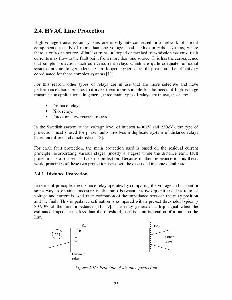
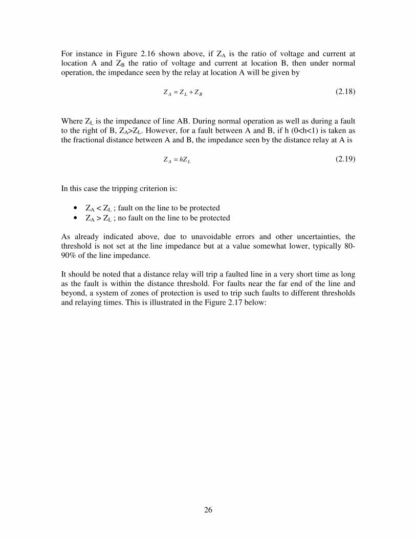
2.4.1. Distance Protection In terms of principle, the distance relay operates by comparing the voltage and current in some way to obtain a measure of the ratio between the two quantities. The ratio of voltage and current is used as an estimation of the impedance between the relay position and the fault. This impedance estimation is compared with a pre-set threshold, typically 80-90% of the line impedance [11, 19]. The relay generates a trip signal when the estimated impedance is less than the threshold, as this is an indication of a fault on the line.

Figure 2.16: Principle of distance protection

Distance relay

Other lines

ZA ZB

26

For instance in Figure 2.16 shown above, if ZA is the ratio of voltage and current at location A and ZB the ratio of voltage and current at location B, then under normal operation, the impedance seen by the relay at location A will be given by

BLA ZZZ += (2.18)

Where ZL is the impedance of line AB. During normal operation as well as during a fault to the right of B, ZA>ZL. However, for a fault between A and B, if h (0<h<1) is taken as the fractional distance between A and B, the impedance seen by the distance relay at A is

LA hZZ = (2.19)

In this case the tripping criterion is:

• ZA < ZL ; fault on the line to be protected • ZA > ZL ; no fault on the line to be protected

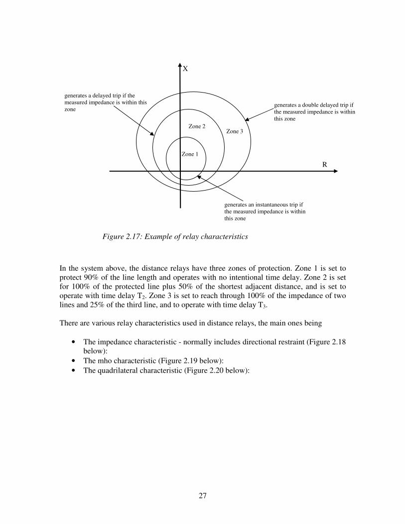
As already indicated above, due to unavoidable errors and other uncertainties, the threshold is not set at the line impedance but at a value somewhat lower, typically 80-90% of the line impedance. It should be noted that a distance relay will trip a faulted line in a very short time as long as the fault is within the distance threshold. For faults near the far end of the line and beyond, a system of zones of protection is used to trip such faults to different thresholds and relaying times. This is illustrated in the Figure 2.17 below:

27

In the system above, the distance relays have three zones of protection. Zone 1 is set to protect 90% of the line length and operates with no intentional time delay. Zone 2 is set for 100% of the protected line plus 50% of the shortest adjacent distance, and is set to operate with time delay T2. Zone 3 is set to reach through 100% of the impedance of two lines and 25% of the third line, and to operate with time delay T3. There are various relay characteristics used in distance relays, the main ones being

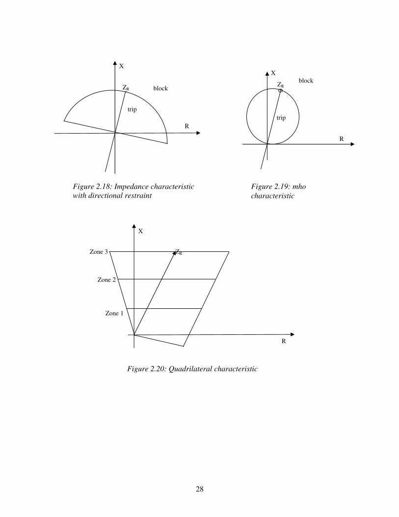
• The impedance characteristic - normally includes directional restraint (Figure 2.18 below):

• The mho characteristic (Figure 2.19 below): • The quadrilateral characteristic (Figure 2.20 below):

generates a double delayed trip if the measured impedance is within this zone

R

X

Zone 1

Zone 2 Zone 3

generates an instantaneous trip if the measured impedance is within this zone

generates a delayed trip if the measured impedance is within this zone

Figure 2.17: Example of relay characteristics

28

Figure 2.19: mho characteristic

trip

block ZR

trip

block ZR

Figure 2.18: Impedance characteristic with directional restraint

R

X

R

R

X X

ZR

Zone 1

Zone 2

Zone 3

Figure 2.20: Quadrilateral characteristic

29

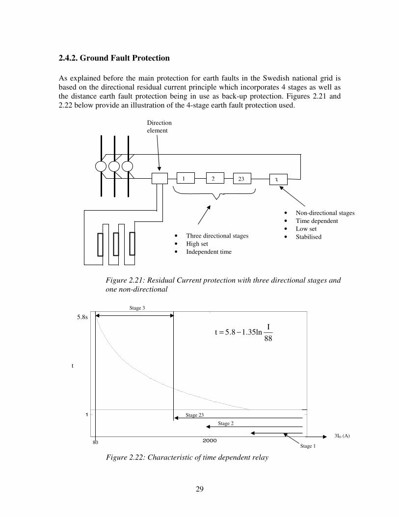
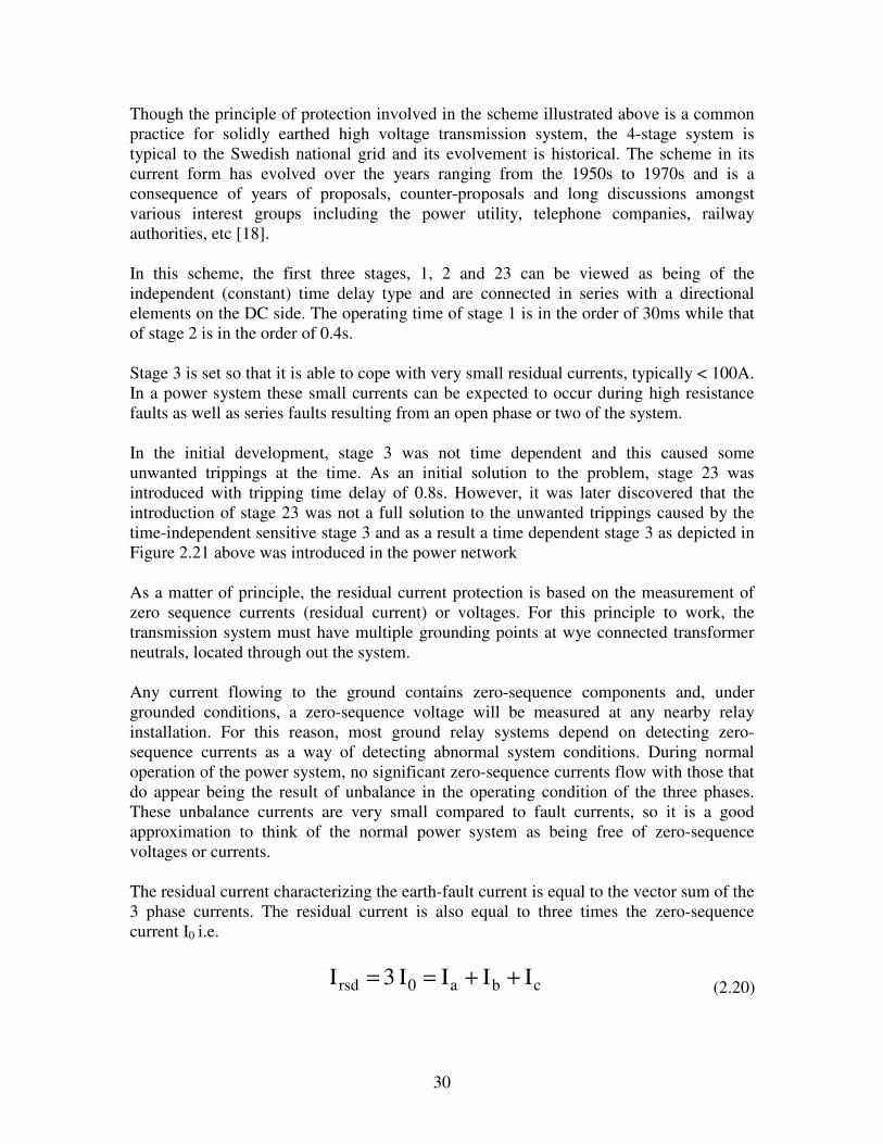
2.4.2. Ground Fault Protection As explained before the main protection for earth faults in the Swedish national grid is based on the directional residual current principle which incorporates 4 stages as well as the distance earth fault protection being in use as back-up protection. Figures 2.21 and 2.22 below provide an illustration of the 4-stage earth fault protection used.

Figure 2.21: Residual Current protection with three directional stages and one non-directional

1 2 23 3

• Three directional stages • High set • Independent time

• Non-directional stages • Time dependent • Low set • Stabilised

Direction element

Figure 2.22: Characteristic of time dependent relay

2000

1

Stage 1

3IO (A)

Stage 3

t

5.8s

88I

35ln.18.5t − =

80

Stage 2

Stage 23

30

Though the principle of protection involved in the scheme illustrated above is a common practice for solidly earthed high voltage transmission system, the 4-stage system is typical to the Swedish national grid and its evolvement is historical. The scheme in its current form has evolved over the years ranging from the 1950s to 1970s and is a consequence of years of proposals, counter-proposals and long discussions amongst various interest groups including the power utility, telephone companies, railway authorities, etc [18]. In this scheme, the first three stages, 1, 2 and 23 can be viewed as being of the independent (constant) time delay type and are connected in series with a directional elements on the DC side. The operating time of stage 1 is in the order of 30ms while that of stage 2 is in the order of 0.4s. Stage 3 is set so that it is able to cope with very small residual currents, typically < 100A. In a power system these small currents can be expected to occur during high resistance faults as well as series faults resulting from an open phase or two of the system. In the initial development, stage 3 was not time dependent and this caused some unwanted trippings at the time. As an initial solution to the problem, stage 23 was introduced with tripping time delay of 0.8s. However, it was later discovered that the introduction of stage 23 was not a full solution to the unwanted trippings caused by the time-independent sensitive stage 3 and as a result a time dependent stage 3 as depicted in Figure 2.21 above was introduced in the power network As a matter of principle, the residual current protection is based on the measurement of zero sequence currents (residual current) or voltages. For this principle to work, the transmission system must have multiple grounding points at wye connected transformer neutrals, located through out the system. Any current flowing to the ground contains zero-sequence components and, under grounded conditions, a zero-sequence voltage will be measured at any nearby relay installation. For this reason, most ground relay systems depend on detecting zero-sequence currents as a way of detecting abnormal system conditions. During normal operation of the power system, no significant zero-sequence currents flow with those that do appear being the result of unbalance in the operating condition of the three phases. These unbalance currents are very small compared to fault currents, so it is a good approximation to think of the normal power system as being free of zero-sequence voltages or currents. The residual current characterizing the earth-fault current is equal to the vector sum of the 3 phase currents. The residual current is also equal to three times the zero-sequence current I0 i.e.

cba0rsd III I 3 I ++ = =

(2.20)

31

where Ia, Ib and Ic are phase currents while I0 and Irsd are the zero sequence and residual currents respectively. In systems where directional overcurrent ground relaying is used, determination of the direction of a fault current is included with the protection system. In order to determine the direction of a fault current from the ground relay location it is necessary to provide the relay with a reference or polarising quantity against which the zero-sequence line (fault) current can be compared, giving the relay a sense of the current direction. The polarising quantity can be either a zero-sequence voltage or current. In Figure 2.21 above a directional element based on voltage polarisation in an open delta arrangement is included and this seems to be typical in the Swedish national grid.

32

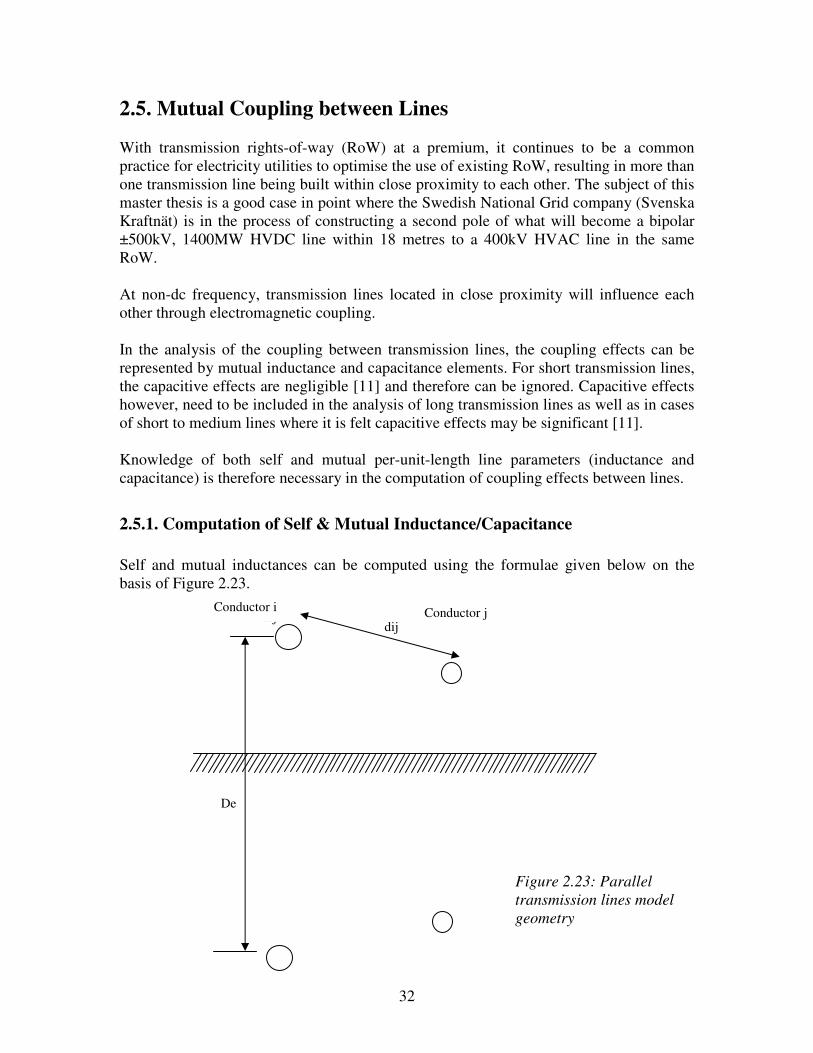
2.5. Mutual Coupling between Lines With transmission rights-of-way (RoW) at a premium, it continues to be a common practice for electricity utilities to optimise the use of existing RoW, resulting in more than one transmission line being built within close proximity to each other. The subject of this master thesis is a good case in point where the Swedish National Grid company (Svenska Kraftnät) is in the process of constructing a second pole of what will become a bipolar ±500kV, 1400MW HVDC line within 18 metres to a 400kV HVAC line in the same RoW. At non-dc frequency, transmission lines located in close proximity will influence each other through electromagnetic coupling. In the analysis of the coupling between transmission lines, the coupling effects can be represented by mutual inductance and capacitance elements. For short transmission lines, the capacitive effects are negligible [11] and therefore can be ignored. Capacitive effects however, need to be included in the analysis of long transmission lines as well as in cases of short to medium lines where it is felt capacitive effects may be significant [11]. Knowledge of both self and mutual per-unit-length line parameters (inductance and capacitance) is therefore necessary in the computation of coupling effects between lines.

2.5.1. Computation of Self & Mutual Inductance/Capacitance Self and mutual inductances can be computed using the formulae given below on the basis of Figure 2.23.

dij dij

De

Conductor i Conductor j

Figure 2.23: Parallel transmission lines model geometry

33

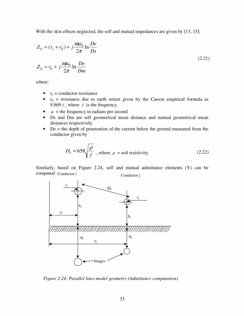
With the skin effects neglected, the self and mutual impedances are given by [13, 15]:

DsDe

jrrZ dcii ln2

)( 0

πωµ

++=

DmDe

jrZ dij ln2

0

πωµ

+=

where:

• rc = conductor resistance • rd = resistance due to earth return given by the Carson empirical formula as

9.869 f , where f is the frequency. • ω = the frequency in radians per second • Ds and Dm are self geometrical mean distance and mutual geometrical mean

distances respectively. • De = the depth of penetration of the current below the ground measured from the

conductor given by

fDe

ρ658= , where ρ = soil resistivity.

Similarly, based on Figure 2.24, self and mutual admittance elements (Y) can be computed:

rj

ri

yj

yi

hi

-hi -hj

hj

dij

Conductor i Conductor j

Images

Figure 2.24: Parallel lines model geometry (Admittance computation)

(2.21)

(2.22)

34

1−= PY

where, P is a matrix (potential coefficients) with its elements given by

ij

jijioij d

hhyyjP

22 )()(ln2

++−= πεω

where 22 )()( jijiij hhyyd −+−= for i j and

dij = radius of conductor i for i = j and o is permittivity of free space. Though in the illustrations above, transmission lines have been shown consisting only of one conductor, the equations as given are general enough and equally apply to multiconductor transmission lines.

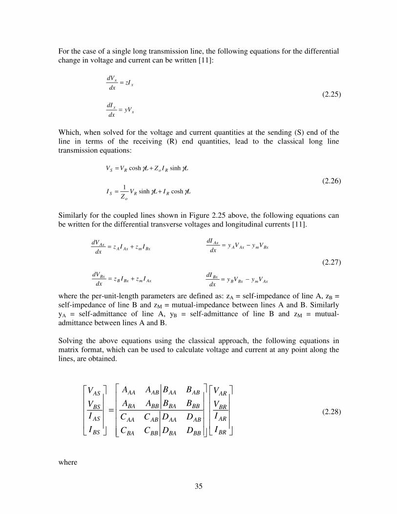
2.5.2. Computation of Coupling Effects With per-unit-length line parameters calculated as in 2.3.2 above, and assuming an electrically long transmission line model, the coupling between the lines can be computed, taking into account the distributed effects of the lines series impedances and shunt admittances. Figure 2.25 below is an illustration of the differential parameters of two mutually coupled long lines. Figure 2.25: Differential parameters for two mutually coupled long lines

zAdx IAx

zmdx

ymdx VAx+ dVAx

+

-

(yB- ym)dx

zBdx

(yA- ym)dx

IBS IBR IBx

+ VAS

-

+ VAR

-

+ VBR

-

+ VBS

-

IAx+ dIAx

IBx+ dIBx

IAS IAR

VBx+ dVBx +

-

x dx

L

(2.23)

(2.24)

35

For the case of a single long transmission line, the following equations for the differential change in voltage and current can be written [11]:

xx zI

dxdV

=

xx yV

dxdI

=

Which, when solved for the voltage and current quantities at the sending (S) end of the line in terms of the receiving (R) end quantities, lead to the classical long line transmission equations:

LIZLVV RoRS γγ sinhcosh +=

LILVZ

I RRo

S γγ coshsinh1 +=

Similarly for the coupled lines shown in Figure 2.25 above, the following equations can be written for the differential transverse voltages and longitudinal currents [11].

where the per-unit-length parameters are defined as: zA = self-impedance of line A, zB = self-impedance of line B and zM = mutual-impedance between lines A and B. Similarly yA = self-admittance of line A, yB = self-admittance of line B and zM = mutual- admittance between lines A and B. Solving the above equations using the classical approach, the following equations in matrix format, which can be used to calculate voltage and current at any point along the lines, are obtained.

=

BR

AR

BR

AR

BBBA

ABAA

BBBA

ABAA

BBBA

ABAA

BBBA

ABAA

BS

AS

BS

AS

I

IV

V

DD

DD

CC

CC

BB

BB

AA

AA

I

IV

V

where

BxmAxAAx IzIz

dxdV

+= BxmAxAAx VyVy

dxdI

−=

AxmBxBBx IzIz

dxdV

+= AxmBxBBx VyVy

dxdI

−=

(2.25)

(2.26)

(2.27)

(2.28)

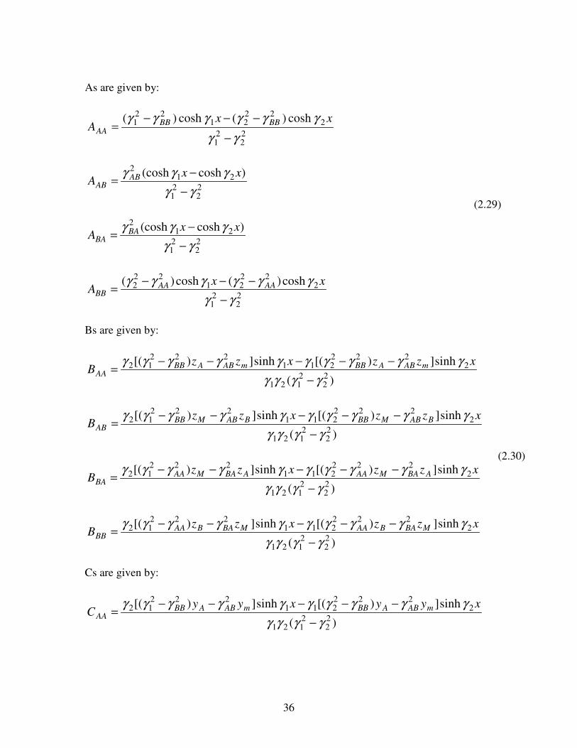
36

As are given by:

22

21

222

2122

1 cosh)(cosh)(

γγγγγγγγ

−−−−

=xx

A BBBBAA

22

21

212 )cosh(cosh

γγγγγ

−−= xx

A ABAB

22

21

212 )cosh(cosh

γγγγγ

−−= xx

A BABA

22

21

222

2122

2 cosh)(cosh)(

γγγγγγγγ

−−−−= xx

A AAAABB

Bs are given by:

)(

sinh])[(sinh])[(22

2121

2222

211222

12

γγγγγγγγγγγγγγ

−−−−−−

=xzzxzz

B mABABBmABABBAA

)(

sinh])[(sinh])[(22

2121

2222

211222

12

γγγγγγγγγγγγγγ

−−−−−−= xzzxzz

B BABMBBBABMBBAB

)(

sinh])[(sinh])[(22

2121

2222

211222

12

γγγγγγγγγγγγγγ

−−−−−−= xzzxzz

B ABAMAAABAMAABA

)(

sinh])[(sinh])[(22

2121

2222

211222

12

γγγγγγγγγγγγγγ

−−−−−−= xzzxzz

B MBABAAMBABAABB

Cs are given by:

)(

sinh])[(sinh])[(22

2121

2222

211222

12

γγγγγγγγγγγγγγ

−−−−−−

=xyyxyy

C mABABBmABABBAA

(2.29)

(2.30)

37

)(

sinh])[(sinh])[(22

2121

2222

211222

12

γγγγγγγγγγγγγγ

−−−−−−= xyyxyy

C BABMBBBABMBBAB

)(

sinh])[(sinh])[(22

2121

2222

211222

12

γγγγγγγγγγγγγγ

−−−−−−= xyyxyy

C ABAMAAABAMAABA

)(

sinh])[(sinh])[(22

2121

2222

211222

12

γγγγγγγγγγγγγγ

−−−−−−= xyyxyy

C MBABAAMBABAABB

Ds are given by

AAAA AD =

BAAB AD =

ABBA AD =

BBBB AD = and

MMAAAA yzyz −=2γ

MMBBBB yzyz −=2γ

BMMAAB yzyz −=2γ

AMMBBA yzyz −=2γ

))((422 221 MBAMBAMMBBAAMMBBAA yyyzzzyzyzyzyzyzyz −−−−++−+=γ

))((422 222 MBAMBAMMBBAAMMBBAA yyyzzzyzyzyzyzyzyz −−−−+−−+=γ

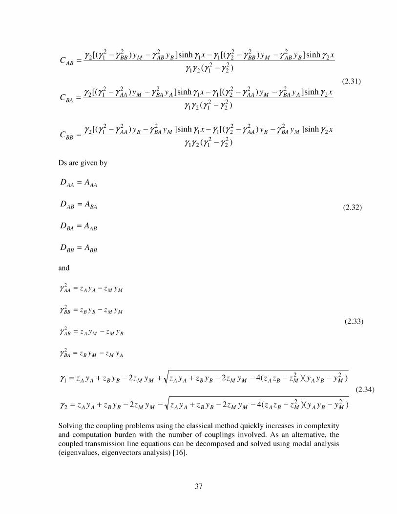
Solving the coupling problems using the classical method quickly increases in complexity and computation burden with the number of couplings involved. As an alternative, the coupled transmission line equations can be decomposed and solved using modal analysis (eigenvalues, eigenvectors analysis) [16].

(2.31)

(2.32)

(2.33)

(2.34)

38

The equations as given above assume that the line is completely transposed and the equations can then be applied to each sequence network in turn. It is well documented in literature that coupling between positive and negative sequence networks of lines is very weak such that it is not uncommon for this aspect to be neglected. However, the coupling between zero sequence networks may be significant and should be subject of detailed analysis [11, 12, 14].

39

3. EXPERIENCES AROUND THE WORLD The problem of coupling between HVAC and HVDC lines has been covered in various scientific papers. Lots of different issues have been covered in these papers, for example induction from AC to DC lines during steady state and fault conditions, induction from a DC line to a neighbouring AC line during transients, influence of AC/DC coupling to different network elements and also different ways about modelling the coupling between lines. Some papers considered the coupling effects if the HVDC and HVAC were placed on the same tower, and others described the problems with these circuits on the same right of way (RoW), but on different towers. The following is a conclusion of important notes from different papers that have covered similar issues to this thesis. 3.1 HVDC Coupling to HVAC This section focuses on the results that were found from three different IEEE scientific papers about the coupling from HVDC lines to HVAC lines. This type of coupling is relevant to the present thesis and is therefore covered more thoroughly than the opposite.

3.1.1. Coupling Case from Reference [5] The paper that covers most similar problems to this thesis is [5]. It concentrates on the cause of large zero sequence transients in AC lines due to transients in a neighbouring earth return DC circuit. The study described in that paper was performed due to tripping of AC lines that shared a common 240 km corridor with two DC circuits in the Manitoba Hydro system in Canada. The reason for tripping the AC lines was the operation of the ground current detection relay. The cause of tripping seemed to be the transition of the DC system from normal metallic return to ground return operation. This phenomenon seemed confusing because a large zero sequence current was observed in the AC line regardless of its distance (183 m) from the DC line. It also seemed to be associated only with a DC line ground current transient, because in steady state no induced current was noted during earth return DC operation. After analyzing the waveforms, it was seen that induction was present at very low frequencies and not at strict DC. This means that if a transition to the ground return operation of a DC circuit has finished and ground return current has decayed to a constant magnitude, no zero sequence currents are induced to the adjacent AC lines. Currents are induced to the AC line only by the transient, which has a fairly low frequency. To study the coupling phenomena, a simple model of the system was built, which represented all the essential parts of the system – ground resistivity and various terminating impedances of the transformer neutrals. In the model, the zero sequence paths of the AC and DC transmission circuits were modelled as two single conductor transmission lines (Figure 3.1). A current of 1 p.u. (at various frequencies) was injected into the DC line which was grounded at the other end. The AC line was terminated with impedances at both ends, which represented the zero sequence impedances at line

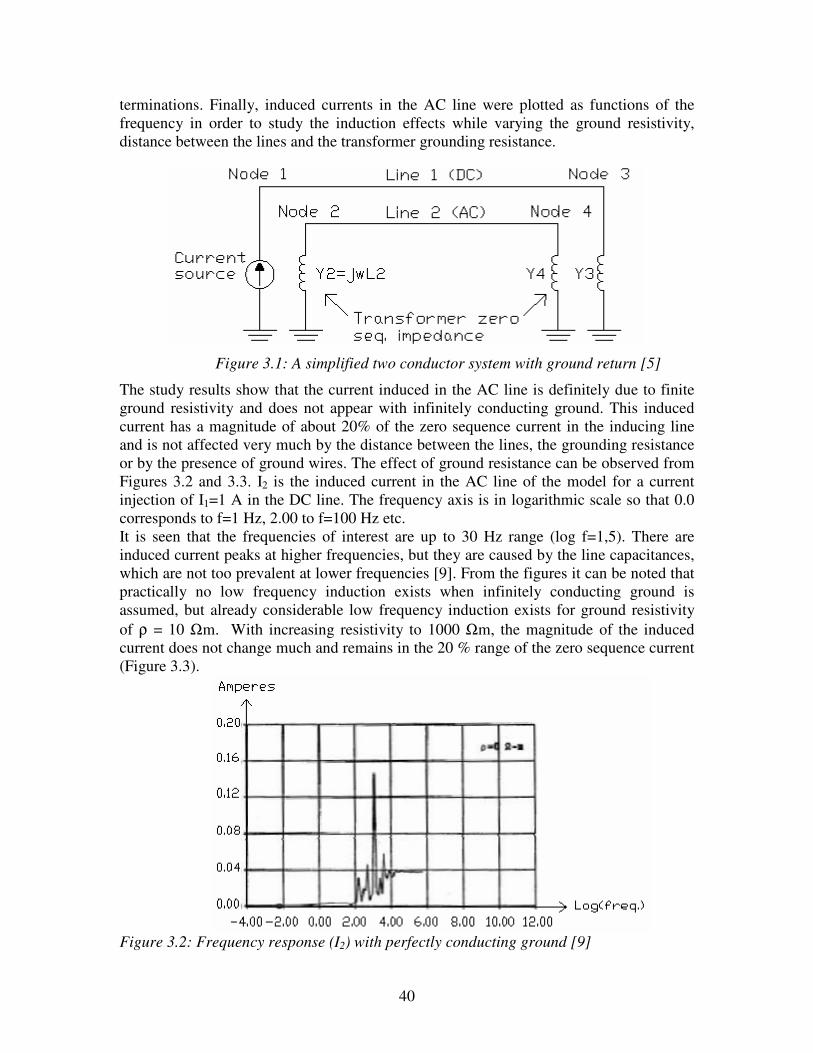
40

terminations. Finally, induced currents in the AC line were plotted as functions of the frequency in order to study the induction effects while varying the ground resistivity, distance between the lines and the transformer grounding resistance.

Figure 3.1: A simplified two conductor system with ground return [5]

The study results show that the current induced in the AC line is definitely due to finite ground resistivity and does not appear with infinitely conducting ground. This induced current has a magnitude of about 20% of the zero sequence current in the inducing line and is not affected very much by the distance between the lines, the grounding resistance or by the presence of ground wires. The effect of ground resistance can be observed from Figures 3.2 and 3.3. I2 is the induced current in the AC line of the model for a current injection of I1=1 A in the DC line. The frequency axis is in logarithmic scale so that 0.0 corresponds to f=1 Hz, 2.00 to f=100 Hz etc. It is seen that the frequencies of interest are up to 30 Hz range (log f=1,5). There are induced current peaks at higher frequencies, but they are caused by the line capacitances, which are not too prevalent at lower frequencies [9]. From the figures it can be noted that practically no low frequency induction exists when infinitely conducting ground is assumed, but already considerable low frequency induction exists for ground resistivity of ρ = 10 Ωm. With increasing resistivity to 1000 Ωm, the magnitude of the induced current does not change much and remains in the 20 % range of the zero sequence current (Figure 3.3).

Figure 3.2: Frequency response (I2) with perfectly conducting ground [9]

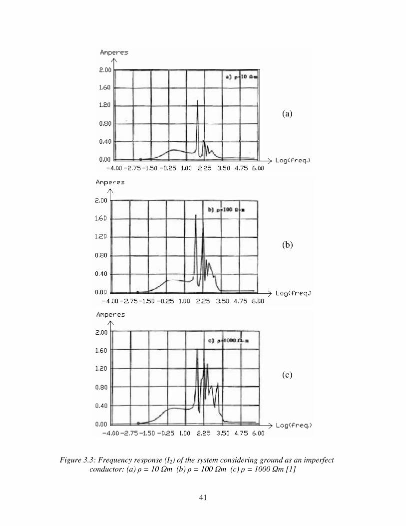
41

Figure 3.3: Frequency response (I2) of the system considering ground as an imperfect conductor: (a) = 10 m (b) = 100 m (c) = 1000 m [1]

(b)

(c)

(a)

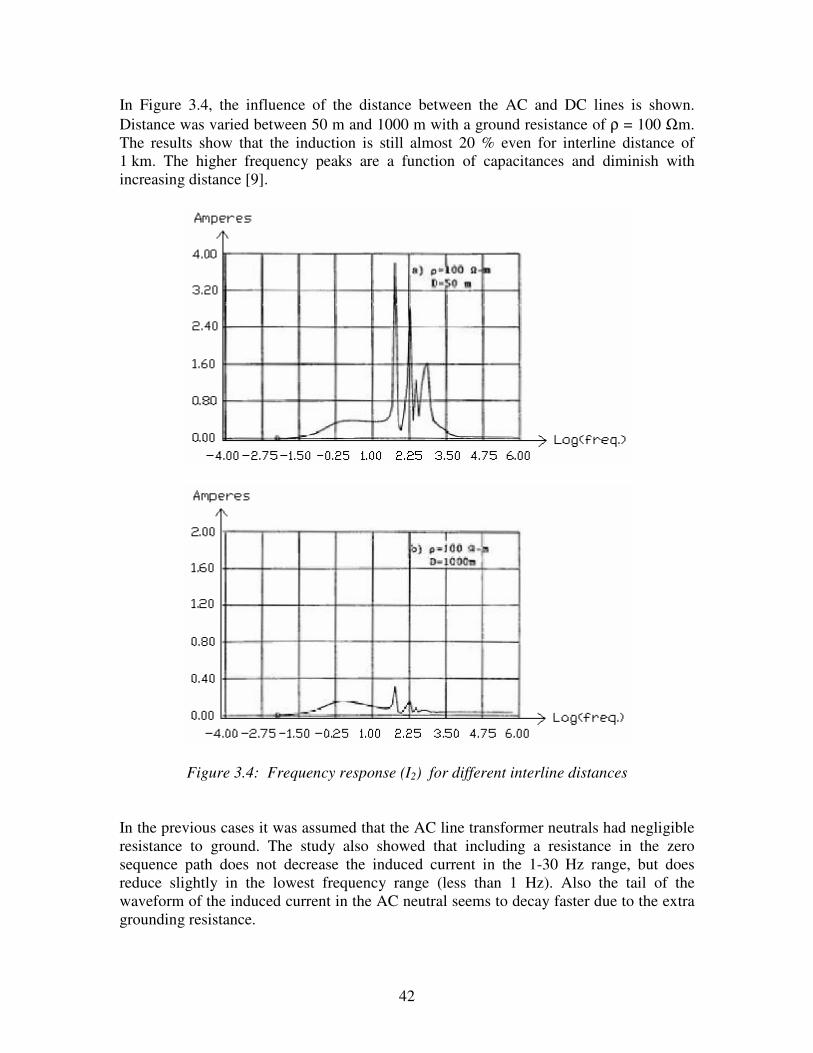
42

In Figure 3.4, the influence of the distance between the AC and DC lines is shown. Distance was varied between 50 m and 1000 m with a ground resistance of ρ = 100 Ωm. The results show that the induction is still almost 20 % even for interline distance of 1 km. The higher frequency peaks are a function of capacitances and diminish with increasing distance [9].

Figure 3.4: Frequency response (I2) for different interline distances In the previous cases it was assumed that the AC line transformer neutrals had negligible resistance to ground. The study also showed that including a resistance in the zero sequence path does not decrease the induced current in the 1-30 Hz range, but does reduce slightly in the lowest frequency range (less than 1 Hz). Also the tail of the waveform of the induced current in the AC neutral seems to decay faster due to the extra grounding resistance.

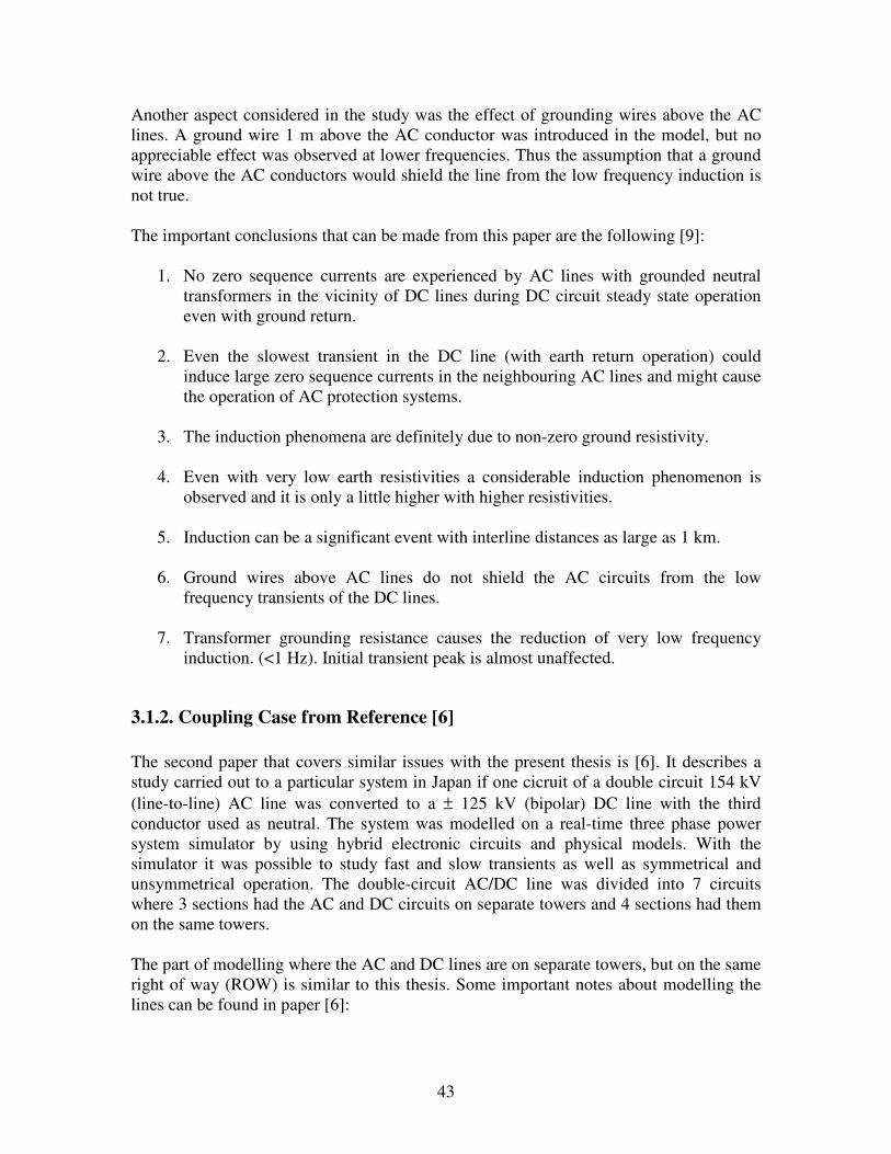
43

Another aspect considered in the study was the effect of grounding wires above the AC lines. A ground wire 1 m above the AC conductor was introduced in the model, but no appreciable effect was observed at lower frequencies. Thus the assumption that a ground wire above the AC conductors would shield the line from the low frequency induction is not true. The important conclusions that can be made from this paper are the following [9]:

1. No zero sequence currents are experienced by AC lines with grounded neutral transformers in the vicinity of DC lines during DC circuit steady state operation even with ground return.

2. Even the slowest transient in the DC line (with earth return operation) could

induce large zero sequence currents in the neighbouring AC lines and might cause the operation of AC protection systems.

3. The induction phenomena are definitely due to non-zero ground resistivity.

4. Even with very low earth resistivities a considerable induction phenomenon is

observed and it is only a little higher with higher resistivities.

5. Induction can be a significant event with interline distances as large as 1 km.

6. Ground wires above AC lines do not shield the AC circuits from the low frequency transients of the DC lines.

7. Transformer grounding resistance causes the reduction of very low frequency

induction. (<1 Hz). Initial transient peak is almost unaffected.

3.1.2. Coupling Case from Reference [6] The second paper that covers similar issues with the present thesis is [6]. It describes a study carried out to a particular system in Japan if one cicruit of a double circuit 154 kV (line-to-line) AC line was converted to a ± 125 kV (bipolar) DC line with the third conductor used as neutral. The system was modelled on a real-time three phase power system simulator by using hybrid electronic circuits and physical models. With the simulator it was possible to study fast and slow transients as well as symmetrical and unsymmetrical operation. The double-circuit AC/DC line was divided into 7 circuits where 3 sections had the AC and DC circuits on separate towers and 4 sections had them on the same towers. The part of modelling where the AC and DC lines are on separate towers, but on the same right of way (ROW) is similar to this thesis. Some important notes about modelling the lines can be found in paper [6]:

44

1. The mutual capacitances between the AC and DC circuits were neglected due to long distance between the lines.

2. It was assumed that the mutual impedances between the conductors of the AC and

DC circuits were all equal due to small inductive coupling and this was represented by placing this impedance on the common ground circuit.

3. The mutual impedances of the same circuit were not equal and the model

accounted for the asymmetrical placement of the conductors.

4. The capacitance model of the AC and DC circuits assumes symmetry between the conductors within the same group.

The paper covered also the modelling of mutual inductances. Useful remarks from the paper are the following:

1. If it can be assumed that mutual inductances are equal, a single inductance can be placed in a common path and can be used instead of several couplings.

2. If the mutual inductances cannot be assumed as equal it is necessary to model all

the inductances individually. To simplify, it can be done by placing an inductance in the common path with the size being less than or equal to the minimum of all mutual inductances. This common inductance can be used for modelling frequency dependence effects.

3. On the simulator in paper [6] the mutual inductances were represented by

transformer-like couplings, but the resistance elements of the mutual impedances were not represented individually. The average of all mutual resistances was taken and placed in the common path.

Different tests were simulated on the hybrid AC/DC line and one of them was a DC line to ground fault. The behaviour of the system was analyzed when a line to ground fault was simulated midway of the positive pole. The fault caused short oscillations which died out in less than 50 ms in the system and it can therefore be said that the response of the system was stable. The fault on one pole did not have any significant influence on the other pole.

3.1.3. Coupling Case from Reference [7] Paper [7] presents the outcome of a feasibility study that was undertaken to examine the AC/HVDC line interactions caused by the close proximity of the transmission lines – AC and DC circuits placed on the same tower. A three-circuit tower configuration was considered in the study – 115 kV AC, 230 kV AC and a bipolar ±500 kV DC.

45

The effects of AC circuits on the DC line as well as DC circuits on the AC line were determined in the study by simulating various faults and loading conditions on both types of lines. Simulations were made with a program called the Alternate Transients Program (ATP) with its associated graphical user-interface ATPDraw. From the simulations it occurred that in the case of a three-phase short circuit on the 230 kV AC line, no appreciable effects were noticed on the DC line’s voltage and current waveforms. But on the other hand, DC faults have appreciable effects on the AC current. When a single pole-to-ground fault occurred on the +500 kV DC line, the current in the AC line had a large negative spike of –375 Apeak compared to the steady state prefault peak-to-peak value of 75 A. After the fault the AC current was still able to recover back to a steady state peak-to-peak value of 75 A. The AC voltage waveform also showed a slight transient response which decayed to zero in less than 0.1 s or 6 cycles. 3.2. HVAC Coupling to HVDC Papers [8], [9] and [10] consider the issues of coupling from AC lines to parallel DC lines. The situations were quite similar in the papers since all of them analyzed AC coupling to DC with the lines being on the same right of way, but on different towers. Lots of similar results can be obtained from these papers. An HVDC line running in parallel with an HVAC line will be exposed to fundamental frequency coupling [6]. A steady state fundamental frequency current will be superimposed on the DC current in the HVDC line due to inductive and capacitive coupling from adjacent AC lines [8]. The induced fundamental frequency current is converted into a DC current and a series of harmonic currents of the sidebands of the converter transformer valve side current [8]. The DC component causes an unsymmetrical magnetization and could lead to converter transformer core saturation during a fraction of the cycle. This causes the noncharacteristic current harmonic, increased noise and transformer heating [8]. Due to the saturation also other undesirable effects are caused, such as [9]:

1. Transformer loss of life due to the localized stray flux heating and possible

deterioration of interlamination insulation caused by the increased magnetostrictive forces.

2. Harmonic generation - a broad spectrum of harmonics is injected into the AC and

DC sides due to the saturation. The high harmonic content makes it difficult to design filters on both the AC and DC sides. High harmonic content is present also in the neutral current of the transformer, which is of primary importance to filter design, because it causes a much higher level of telephone interference than the same amount of current flowing in a balanced mode of the transmission line.

46

3. Control and protection - due to the presence of a DC component the current transformers will experience a similar offset saturation, which leads to inaccurate measurements of current. In the DC control, CT saturation may lead to optimistic measurements of extinction angle and can cause the operation with lower extinction angle than planned. This results in the control of being more prone to commutation failures with minor system disturbances. By the CT measurement errors the transformer differential protection can be affected, resulting in either decreased sensitivity or false trips.

Paper [10] states that the driving sources of fundamental frequency current in the DC line are voltages and currents in the AC line, which can be represented by their sequence components, but only three of them need to be considered in the model:

1. Positive-sequence voltage

2. Positive-sequence current

3. Zero-sequence current Explanation for neglecting 3 components is the following. Positive-sequence components are important due to their magnitudes – close to 1 pu. Negative-sequence components obey the same coupling mechanisms as positive, but are small compared to positive-sequence and can be neglected. Zero-sequence voltage is also small and doesn’t couple much current on the DC line. Zero-sequence currents are also small, but their contribution cannot be neglected, because these currents return through ground or via overhead ground wires [10]. The most important results from the simulations are the following:

1. Distance between AC and DC lines and the length of paralleling are dominating factors in the strength of coupling [10].

2. Higher resistivity of earth may result in stronger capacitive coupling [10].

3. If the steady state fundamental component of DC current ripple was kept below

0.1% of the converter rating, the HVDC system performance is not effected substantially. A fundamental component of 1% would cause a noticeable impact upon the system performance. If the threshold of 0.1% of the fundamental frequency induction is exceeded, studies of the effect on converter performance should be required [9].

Possibilities to mitigate the problem of fundamental frequency induction are the use of DC filters, modulation of DC control, transposing AC and DC lines [9].

47

4. SYSTEM MODEL IN PSCAD This chapter describes the system model developed in PSCAD/EMTDC and used for studying the coupling phenomenon involving AC lines due to a line-to-ground fault occurring on the DC line. The digital simulator used for studies, PSCAD/EMTDC, is a time-domain transient simulator, which can be used in simulating a power system and its controls. It comes with a graphical user interface for sketching electrical equipment and provides a fast and flexible solution. This digital simulator represents and solves differential equations of the entire power system and its control in time domain. The overview of the system setup in PSCAD/EMTDC is shown in Figure 4.1 below. The system can be viewed as consisting of three main blocks namely, the HVDC system, the HVAC lines together with their terminating impedances and the AC/DC line coupled sections. Though the subject of this thesis focuses on studying the coupling phenomenon to the AC lines due to a pole-to-ground fault occurring on the DC line, a great deal of time and effort was devoted to the modelling, validation and testing of the HVDC system. This was necessary to ensure that the performance of the HVDC system was as close as possible to the real system and therefore ensure that the coupling results obtained would closely match what could be expected to happen in reality. Despite the fact that no calibration of the model with the actual system was carried out, based on a comparison of known inputs and their corresponding outputs, the authors believe this goal was achieved within tolerable error margins. The model description includes the following elements:

a) The HVDC System – under this subheading the following components are covered; the AC System, The converter transformers, the converters, the DC side, the AC filters and the control system.

b) The HVAC lines c) The DC/AC line coupled sections

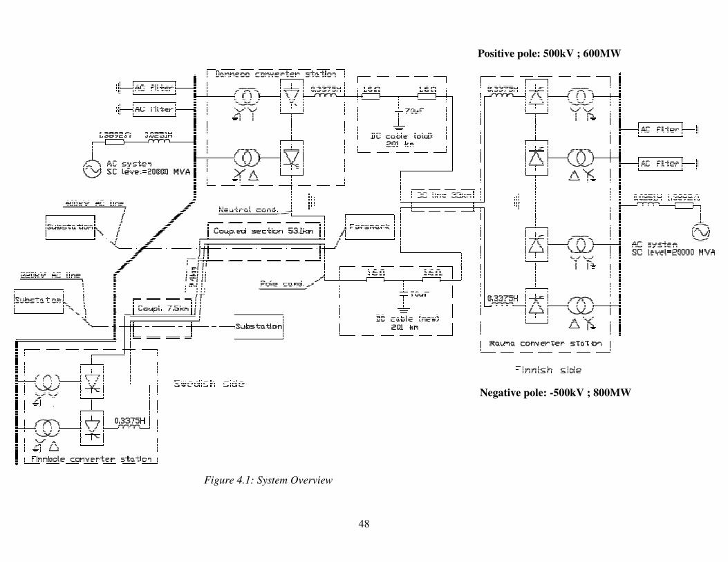
48

Figure 4.1: System Overview

Positive pole: 500kV ; 600MW

Negative pole: -500kV ; 800MW

49

4.1. HVDC System As can be seen in Figure 4.1, the HVDC system has been modelled as a ±500kV, 1400MW bipolar connection between the Swedish and Finnish power systems. This is in agreement with the expansion plans currently being worked on by Svenska Kraftnät and Fingrid. The positive pole (existing pole) of the bipolar system has been modelled with a power rating of 600MW, while the negative pole (new pole) has a power rating of 800MW. In modelling the HVDC system the CIGRE HVDC benchmark system available as an example file in PSCAD/EMTDC was employed as the basis for building the model used in this study. The HVDC system model is therefore quite detailed, taking into account component details for both the Swedish and Finnish AC systems including the AC filters, converter transformers, converters, the DC side system and the rectifier and inverter control systems.

4.1.1. The AC Systems The AC sides of the HVDC system on the Swedish and Finnish ends have been modelled consisting of supply networks incorporating AC side filters. The AC networks at both ends have been represented by Thevenin equivalent voltage sources with equivalent source impedances (voltage source behind impedance). Source impedances were computed based on short circuit levels for the converter AC substations provided by the Swedish and Finnish transmission operators. The system fault levels for the two AC substations as provided by the two utilities are indicated in Table 4.1 below. The impedance angles at both system ends were selected to be 80 degrees as this is likely to be more representative in the case of resonance at low frequencies [3]. Table 4.1: Fault levels at AC substations

Description Swedish Side (MVA)

Finish Side (MVA)

1 Minimum short circuit capacity 8000 3000 2 Max. symmetrical short circuit capacity 20000 13000 3 Future maximum short circuit capacity 25000 20000

On the basis of the information in the table above a short circuit level of 20GVA was adopted for both the HVDC AC terminals in the base case and a parametric study was carried out using other values to determine whether a change in short circuit level would impact the study results.

4.1.2. Converter Transformers Each 12 pulse converter side has been modelled consisting of two three-phase two winding transformers, one with a grounded Wye-Wye connection and the other one with a grounded Wye-Delta connection. In the absence of actual transformer parameters, the transformer parameters adopted are considered typical for transformers found in HVDC

50

installations. A leakage reactance of 18% (X =0.18 p.u.) was adopted for all transformers. The transformer power ratings were determined to be 2x370MVA and 2x494MVA for the positive and negative poles respectively using the calculation method detailed below. Secondary side rated Voltage:

2cos

1

232

CNBR

drr X

N

VV

−⋅=

α

π (4.1)

and secondary side fundamental RMS rated current:

dNr II ⋅=32

2 (4.2)

and transformer MVA Rating:

rrr IVS 222 3 ⋅⋅= (4.3) where NBR = number of six pulse bridges, XC = commutating reactance, Vdr = DC nominal voltage at the rectifier (an appropriate value should be used if the calculation is done for the inverter), IdN = DC nominal current.

4.1.3. Converters All converters used in the model are in accordance with the PSCAD/EMTDC simulator six-pulse Graetz bridge block, which includes an internal Phase Locked Oscillator (PLO), firing and valve blocking controls, and firing angle () / extinction angle () measurements. They also included built-in RC snubber circuits for each thyristor. The thyristor valves are modelled as ideal devices and therefore, negative turn-off and firing due to large (dv/dt) and (di/dt) are not considered.

4.1.4. The DC Side The DC sides for the two poles of the HVDC link, though having some similarities, have been modelled differently mainly due to the fact that the negative pole (new pole) incorporates an overhead DC line of about 70km on the Swedish side, which shares rights-of-way with a 400kV AC line for 53km and a 220kV AC line for 7.5km. The positive pole (existing pole) DC side model consists of smoothing reactors at the two HVDC ends (inverter and rectifier) and a 200km undersea cable running from Sweden (Dannebo) and transforming into a 33km overhead line before terminating in the converter station on the Finnish side (Rauma).

51

The negative pole (new pole) DC side model, just like the positive pole, consists of smoothing reactors at the two HVDC ends (inverter and rectifier) and a 200km undersea cable running from Sweden and transforming into a 33km overhead line before terminating in the converter station on the Finnish side (Rauma station). However this pole also consists of a 70km overhead DC line section connecting the undersea cable to the negative pole converter station (Finnböle station) on the Swedish side. The tower for this overhead line section is also used to carry the return conductor running in between the two converter stations on the Swedish side and connected to the earth electrode located near Dannebo and the Baltic sea. In the model equally sized smoothing reactors (0.3375 H) have been used at each end for both poles. The sizes of the smoothing reactors are equivalent to that currently installed on the existing pole (positive pole in Figure 4.1) of the HVDC system. The undersea cables of the DC links have been represented by an equivalent T-network, similar to the implementation in the Cigre benchmark model. The cable resistance and capacitance values used were provided by Svenska Kraftnät. Given that the overhead line section of the negative pole (new pole) will run in parallel with the 400kV and 220kV AC lines in areas where it will share the same rights-of-way with these lines, its modelling has been based on the frequency dependent (phase) model found in PSCAD/EMTDC. As also explained in Section 4.3 below of this chapter, this line representation gives the most accurate results for transient-type studies. Details of all overhead lines used in the study are provided in Appendix 1.

4.1.5. AC Filters & Reactive Compensations As shown in Figure 4.1, tuned filters were incorporated for filtering out harmonics generated by the HVDC system at both ends of the system. The most relevant harmonics are of the orders of 11, 13 and the higher characteristic harmonics (multiples of 11 and 13). The parameters and impedance characteristic of the AC filters at the rectifier and inverter end AC systems are provided in Appendix 2. The total reactive power consumption of the converters at each end of the HVDC system is about 640MVAr. This reactive power is supplied by the filters in the model.

4.1.6. The Control Systems The controls for the HVDC system are identical for both the positive and negative poles and are modelled independent of each other. No bipolar or higher level controls are incorporated in the system. The desired power levels are determined by the voltage and current levels in the DC lines. The voltages in the system are determined by the secondary voltages of the converter transformers and the firing angles of the converter bridges. The steady state firing angle for the rectifier is chosen as 20º and the extinction angle for the inverter as 15º. The current levels in the model are given manually as references – 1,2 kA and 1,6 kA for the positive and negative poles respectively. Since

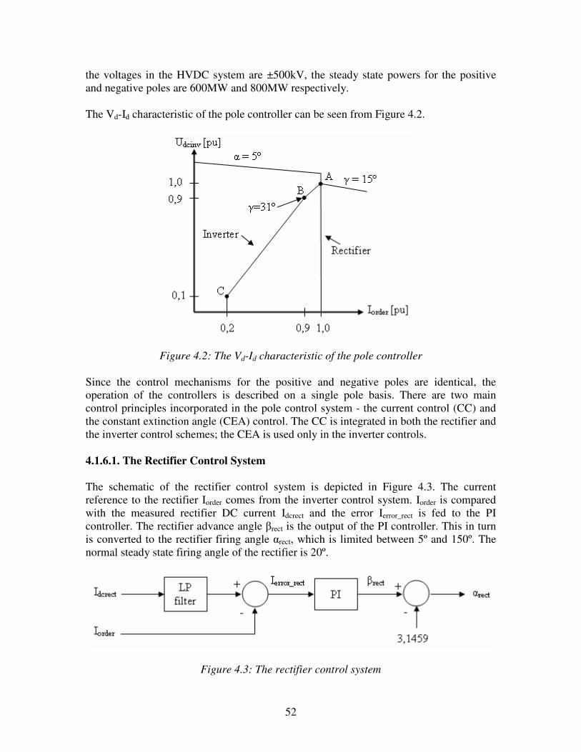
52

the voltages in the HVDC system are ±500kV, the steady state powers for the positive and negative poles are 600MW and 800MW respectively. The Vd-Id characteristic of the pole controller can be seen from Figure 4.2.

Figure 4.2: The Vd-Id characteristic of the pole controller Since the control mechanisms for the positive and negative poles are identical, the operation of the controllers is described on a single pole basis. There are two main control principles incorporated in the pole control system - the current control (CC) and the constant extinction angle (CEA) control. The CC is integrated in both the rectifier and the inverter control schemes; the CEA is used only in the inverter controls. 4.1.6.1. The Rectifier Control System The schematic of the rectifier control system is depicted in Figure 4.3. The current reference to the rectifier Iorder comes from the inverter control system. Iorder is compared with the measured rectifier DC current Idcrect and the error Ierror_rect is fed to the PI controller. The rectifier advance angle rect is the output of the PI controller. This in turn is converted to the rectifier firing angle rect, which is limited between 5º and 150º. The normal steady state firing angle of the rectifier is 20º.

Figure 4.3: The rectifier control system

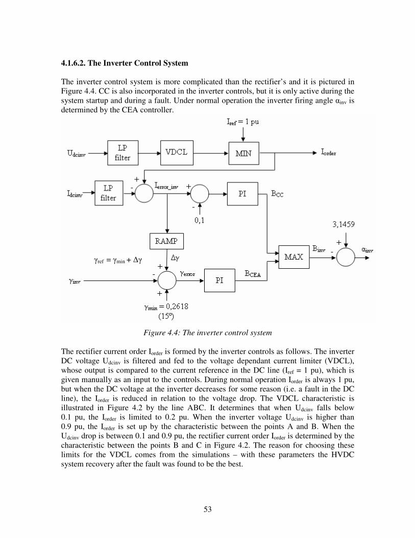
53

4.1.6.2. The Inverter Control System The inverter control system is more complicated than the rectifier’s and it is pictured in Figure 4.4. CC is also incorporated in the inverter controls, but it is only active during the system startup and during a fault. Under normal operation the inverter firing angle inv is determined by the CEA controller.

Figure 4.4: The inverter control system

The rectifier current order Iorder is formed by the inverter controls as follows. The inverter DC voltage Udcinv is filtered and fed to the voltage dependant current limiter (VDCL), whose output is compared to the current reference in the DC line (Iref = 1 pu), which is given manually as an input to the controls. During normal operation Iorder is always 1 pu, but when the DC voltage at the inverter decreases for some reason (i.e. a fault in the DC line), the Iorder is reduced in relation to the voltage drop. The VDCL characteristic is illustrated in Figure 4.2 by the line ABC. It determines that when Udcinv falls below 0.1 pu, the Iorder is limited to 0.2 pu. When the inverter voltage Udcinv is higher than 0.9 pu, the Iorder is set up by the characteristic between the points A and B. When the Udcinv drop is between 0.1 and 0.9 pu, the rectifier current order Iorder is determined by the characteristic between the points B and C in Figure 4.2. The reason for choosing these limits for the VDCL comes from the simulations – with these parameters the HVDC system recovery after the fault was found to be the best.

ref = min +

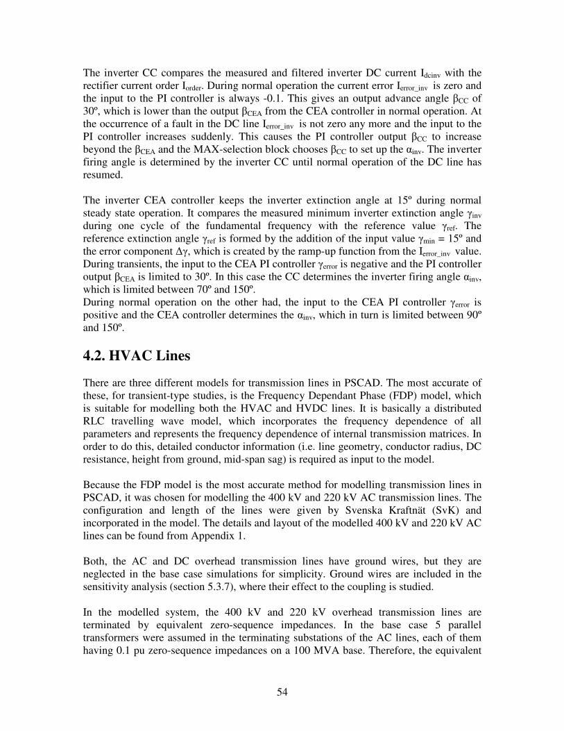
54

The inverter CC compares the measured and filtered inverter DC current Idcinv with the rectifier current order Iorder. During normal operation the current error Ierror_inv is zero and the input to the PI controller is always -0.1. This gives an output advance angle CC of 30º, which is lower than the output CEA from the CEA controller in normal operation. At the occurrence of a fault in the DC line Ierror_inv is not zero any more and the input to the PI controller increases suddenly. This causes the PI controller output CC to increase beyond the CEA and the MAX-selection block chooses CC to set up the inv. The inverter firing angle is determined by the inverter CC until normal operation of the DC line has resumed. The inverter CEA controller keeps the inverter extinction angle at 15º during normal steady state operation. It compares the measured minimum inverter extinction angle inv during one cycle of the fundamental frequency with the reference value ref. The reference extinction angle ref is formed by the addition of the input value min = 15º and the error component , which is created by the ramp-up function from the Ierror_inv value. During transients, the input to the CEA PI controller error is negative and the PI controller output CEA is limited to 30º. In this case the CC determines the inverter firing angle inv, which is limited between 70º and 150º. During normal operation on the other had, the input to the CEA PI controller error is positive and the CEA controller determines the inv, which in turn is limited between 90º and 150º. 4.2. HVAC Lines There are three different models for transmission lines in PSCAD. The most accurate of these, for transient-type studies, is the Frequency Dependant Phase (FDP) model, which is suitable for modelling both the HVAC and HVDC lines. It is basically a distributed RLC travelling wave model, which incorporates the frequency dependence of all parameters and represents the frequency dependence of internal transmission matrices. In order to do this, detailed conductor information (i.e. line geometry, conductor radius, DC resistance, height from ground, mid-span sag) is required as input to the model. Because the FDP model is the most accurate method for modelling transmission lines in PSCAD, it was chosen for modelling the 400 kV and 220 kV AC transmission lines. The configuration and length of the lines were given by Svenska Kraftnät (SvK) and incorporated in the model. The details and layout of the modelled 400 kV and 220 kV AC lines can be found from Appendix 1. Both, the AC and DC overhead transmission lines have ground wires, but they are neglected in the base case simulations for simplicity. Ground wires are included in the sensitivity analysis (section 5.3.7), where their effect to the coupling is studied. In the modelled system, the 400 kV and 220 kV overhead transmission lines are terminated by equivalent zero-sequence impedances. In the base case 5 parallel transformers were assumed in the terminating substations of the AC lines, each of them having 0.1 pu zero-sequence impedances on a 100 MVA base. Therefore, the equivalent

55

zero sequence impedance x0eqv in the terminating substations of the AC lines is the following:

Ω=×=×= 325/)100400

1.0(/)(22

00 transfbase

basepueqv N

SV

xx (4.4)

where x0pu is the zero-sequence impedance of a single transformer, Ntransf is the number of parallel transformers, Vbase and Sbase are the base voltage and power respectively. The value of the equivalent zero-sequence inductance L0eqv can be calculated as follows:

H 0.10.1019502

322

00 ≈=

××==

ππf

xL eqv

eqv (4.5)

where L0eqv is the value used in the base model for terminating the 400 kV and 220 kV AC lines; the zero-sequence resistance is neglected, because its value is much smaller than the reactance. The effect of various terminating impedances to the current that is coupled into the AC lines is analyzed in Section 5.3.5. 4.3. AC/DC Line Coupled Sections The FDP model takes into consideration the mutual coupling between two transmission lines if they are modelled in the same right-of-way (RoW) and it is also capable of accurately simulating the undesirable interactions between DC and AC lines in proximity to one another. Therefore it was decided to choose this model for simulating the coupling between the Dannebo–Finnböle HVDC line and the parallel 220kV and 400kV AC lines. More information about the FDP model and its calculation methods can be found in the PSCAD help file. In order to model more than one transmission line in a single RoW, the distance between the centres of the lines must be specified. Another important parameter is the ground resistivity of the RoW, this must also be given as an input. The rest is similar to modelling a single line – detailed information of the lines (configuration and conductor data) must be given to PSCAD before it calculates the transmission matrices, taking into account the mutual coupling between the modelled lines.

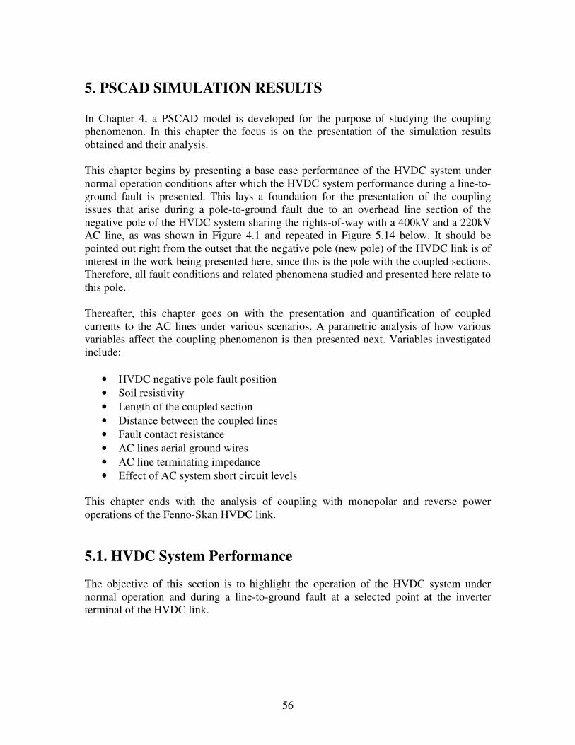
56

5. PSCAD SIMULATION RESULTS In Chapter 4, a PSCAD model is developed for the purpose of studying the coupling phenomenon. In this chapter the focus is on the presentation of the simulation results obtained and their analysis. This chapter begins by presenting a base case performance of the HVDC system under normal operation conditions after which the HVDC system performance during a line-to-ground fault is presented. This lays a foundation for the presentation of the coupling issues that arise during a pole-to-ground fault due to an overhead line section of the negative pole of the HVDC system sharing the rights-of-way with a 400kV and a 220kV AC line, as was shown in Figure 4.1 and repeated in Figure 5.14 below. It should be pointed out right from the outset that the negative pole (new pole) of the HVDC link is of interest in the work being presented here, since this is the pole with the coupled sections. Therefore, all fault conditions and related phenomena studied and presented here relate to this pole. Thereafter, this chapter goes on with the presentation and quantification of coupled currents to the AC lines under various scenarios. A parametric analysis of how various variables affect the coupling phenomenon is then presented next. Variables investigated include:

• HVDC negative pole fault position • Soil resistivity • Length of the coupled section • Distance between the coupled lines • Fault contact resistance • AC lines aerial ground wires • AC line terminating impedance • Effect of AC system short circuit levels

This chapter ends with the analysis of coupling with monopolar and reverse power operations of the Fenno-Skan HVDC link. 5.1. HVDC System Performance The objective of this section is to highlight the operation of the HVDC system under normal operation and during a line-to-ground fault at a selected point at the inverter terminal of the HVDC link.

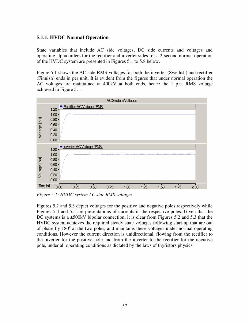
57

5.1.1. HVDC Normal Operation State variables that include AC side voltages, DC side currents and voltages and operating alpha orders for the rectifier and inverter sides for a 2-second normal operation of the HVDC system are presented in Figures 5.1 to 5.8 below. Figure 5.1 shows the AC side RMS voltages for both the inverter (Swedish) and rectifier (Finnish) ends in per unit. It is evident from the figures that under normal operation the AC voltages are maintained at 400kV at both ends, hence the 1 p.u. RMS voltage achieved in Figure 5.1.

AC System Voltages

Time [s] 0.00 0.25 0.50 0.75 1.00 1.25 1.50 1.75 2.00 ... ...

0.00 0.20 0.40 0.60 0.80 1.00 1.20

Vol

tage

[pu

]

Rectifier AC Voltage (RMS)

0.00 0.20 0.40 0.60 0.80 1.00 1.20

Vol

tage

[pu

]

Inverter AC Voltage (RMS)

Figure 5.1: HVDC system AC side RMS voltages Figures 5.2 and 5.3 depict voltages for the positive and negative poles respectively while Figures 5.4 and 5.5 are presentations of currents in the respective poles. Given that the DC systems is a ±500kV bipolar connection, it is clear from Figures 5.2 and 5.3 that the HVDC system achieves the required steady state voltages following start-up that are out of phase by 180o at the two poles, and maintains these voltages under normal operating conditions. However the current direction is unidirectional, flowing from the rectifier to the inverter for the positive pole and from the inverter to the rectifier for the negative pole, under all operating conditions as dictated by the laws of thyristors physics.

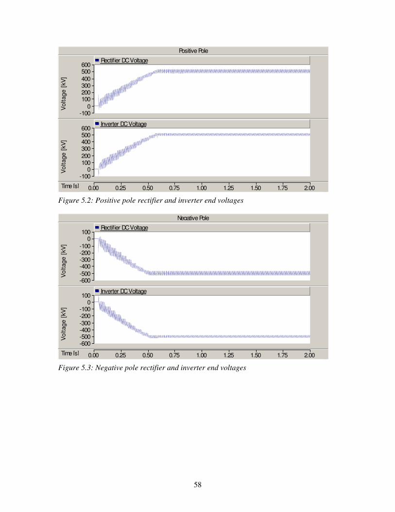
58

Positive Pole

Time [s] 0.00 0.25 0.50 0.75 1.00 1.25 1.50 1.75 2.00 ... ...

-100 0

100 200 300 400 500 600

Vol

tage

[kV

]Rectifier DC Voltage

-100 0

100 200 300 400 500 600

Vol

tage

[kV

]

Inverter DC Voltage

Figure 5.2: Positive pole rectifier and inverter end voltages

Negative Pole

Time [s] 0.00 0.25 0.50 0.75 1.00 1.25 1.50 1.75 2.00 ... ...

-600 -500 -400 -300 -200 -100

0 100

Vol

tage

[kV

]

Rectifier DC Voltage

-600 -500 -400 -300 -200 -100

0 100

Vol

tage

[kV

]

Inverter DC Voltage

Figure 5.3: Negative pole rectifier and inverter end voltages

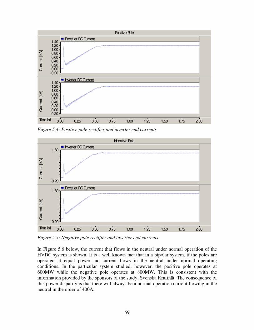
59

Positive Pole

Time [s] 0.00 0.25 0.50 0.75 1.00 1.25 1.50 1.75 2.00 ... ...

-0.20 0.00 0.20 0.40 0.60 0.80 1.00 1.20 1.40

Cur

rent

[kA

]Rectifier DC Current

-0.20 0.00 0.20 0.40 0.60 0.80 1.00 1.20 1.40

Cur

rent

[kA

]

Inverter DC Current

Figure 5.4: Positive pole rectifier and inverter end currents

Negative Pole

Time [s] 0.00 0.25 0.50 0.75 1.00 1.25 1.50 1.75 2.00 ... ...

-0.20

1.80

Cur

rent

[kA

]

Inverter DC Current

-0.20

1.80

Cur

rent

[kA

]

Rectifier DC Current

Figure 5.5: Negative pole rectifier and inverter end currents In Figure 5.6 below, the current that flows in the neutral under normal operation of the HVDC system is shown. It is a well known fact that in a bipolar system, if the poles are operated at equal power, no current flows in the neutral under normal operating conditions. In the particular system studied, however, the positive pole operates at 600MW while the negative pole operates at 800MW. This is consistent with the information provided by the sponsors of the study, Svenska Kraftnät. The consequence of this power disparity is that there will always be a normal operation current flowing in the neutral in the order of 400A.

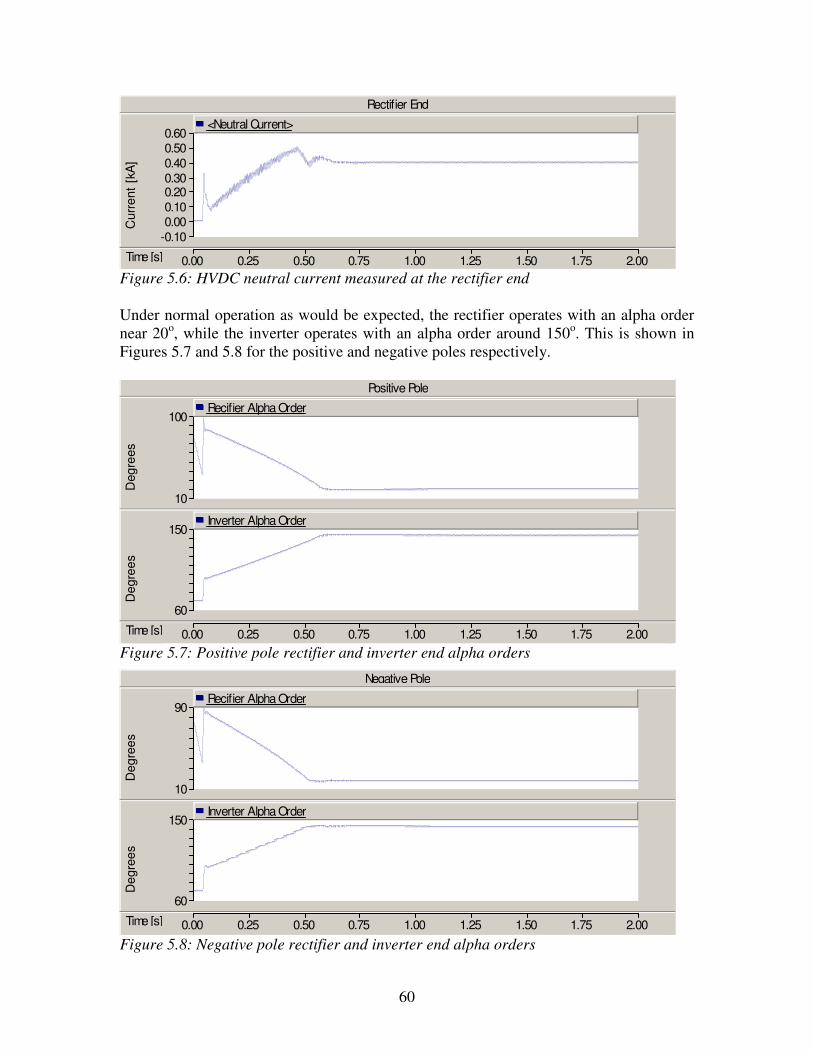
60

Rectifier End

Time [s] 0.00 0.25 0.50 0.75 1.00 1.25 1.50 1.75 2.00 ... ...

-0.10 0.00 0.10 0.20 0.30 0.40 0.50 0.60

Cur

rent

[kA

]<Neutral Current>

Figure 5.6: HVDC neutral current measured at the rectifier end Under normal operation as would be expected, the rectifier operates with an alpha order near 20o, while the inverter operates with an alpha order around 150o. This is shown in Figures 5.7 and 5.8 for the positive and negative poles respectively.

Positive Pole

Time [s] 0.00 0.25 0.50 0.75 1.00 1.25 1.50 1.75 2.00 ... ...

10

100

Deg

rees

Recifier Alpha Order

60

150

Deg

rees

Inverter Alpha Order

Figure 5.7: Positive pole rectifier and inverter end alpha orders

Negative Pole

Time [s] 0.00 0.25 0.50 0.75 1.00 1.25 1.50 1.75 2.00 ... ...

10

90

Deg

rees

Recifier Alpha Order

60

150

Deg

rees

Inverter Alpha Order

Figure 5.8: Negative pole rectifier and inverter end alpha orders

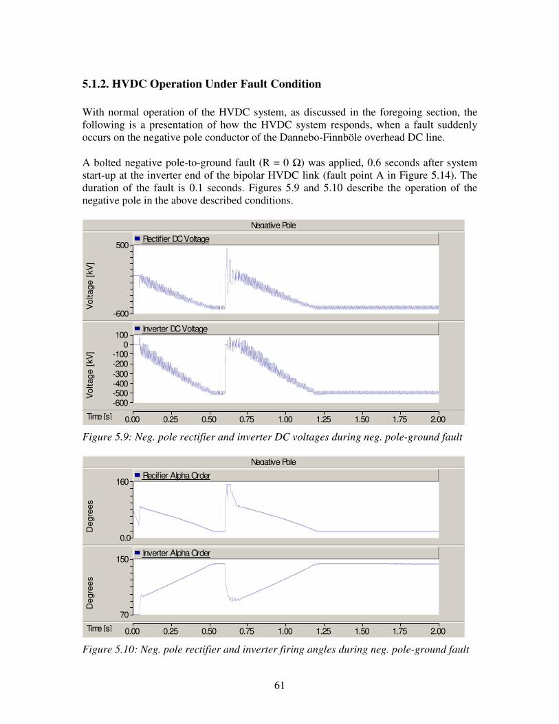
61

5.1.2. HVDC Operation Under Fault Condition With normal operation of the HVDC system, as discussed in the foregoing section, the following is a presentation of how the HVDC system responds, when a fault suddenly occurs on the negative pole conductor of the Dannebo-Finnböle overhead DC line. A bolted negative pole-to-ground fault (R = 0 ) was applied, 0.6 seconds after system start-up at the inverter end of the bipolar HVDC link (fault point A in Figure 5.14). The duration of the fault is 0.1 seconds. Figures 5.9 and 5.10 describe the operation of the negative pole in the above described conditions.

Negative Pole

Time [s] 0.00 0.25 0.50 0.75 1.00 1.25 1.50 1.75 2.00 ... ...

-600

500

Vol

tage

[kV

]

Rectifier DC Voltage

-600 -500 -400 -300 -200 -100

0 100

Vol

tage

[kV

]

Inverter DC Voltage

Figure 5.9: Neg. pole rectifier and inverter DC voltages during neg. pole-ground fault

Negative Pole

Time [s] 0.00 0.25 0.50 0.75 1.00 1.25 1.50 1.75 2.00 ... ...

0.0

160

Deg

rees

Recifier Alpha Order

70

150

Deg

rees

Inverter Alpha Order

Figure 5.10: Neg. pole rectifier and inverter firing angles during neg. pole-ground fault

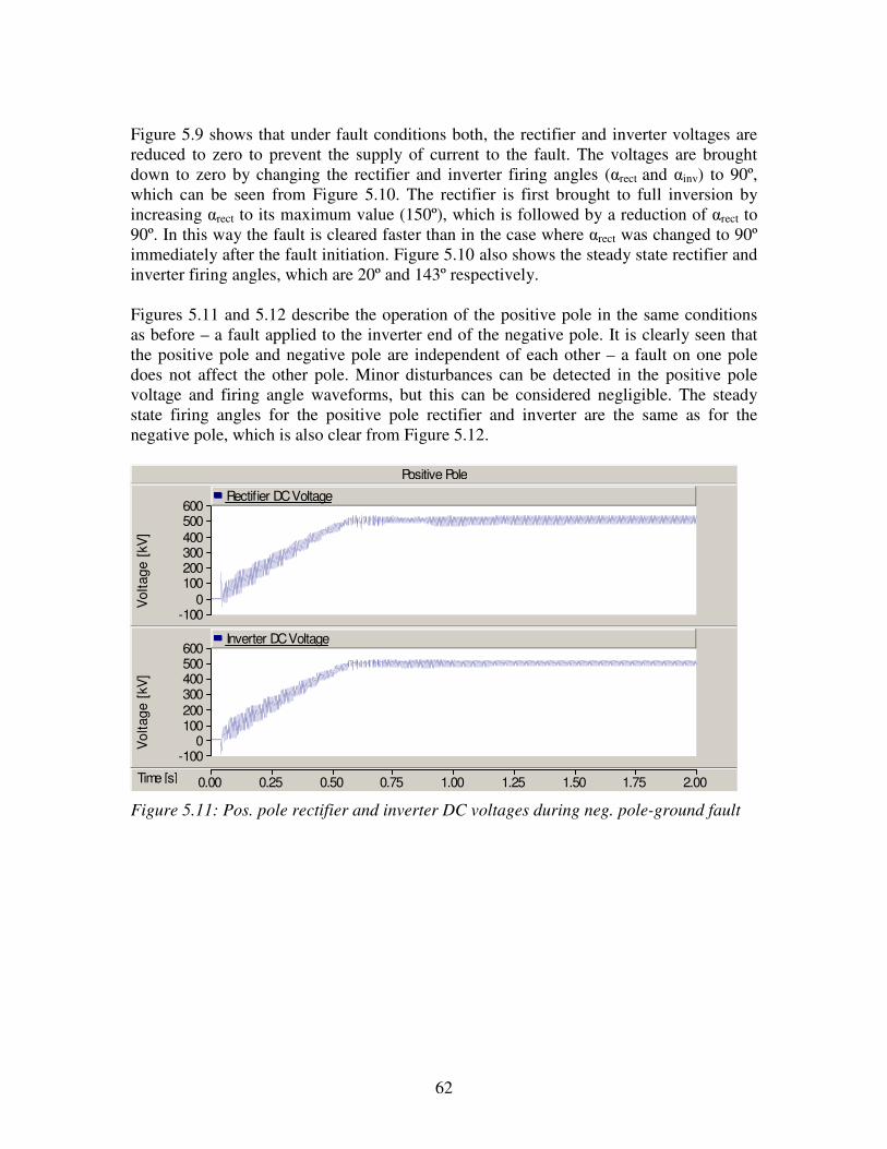
62

Figure 5.9 shows that under fault conditions both, the rectifier and inverter voltages are reduced to zero to prevent the supply of current to the fault. The voltages are brought down to zero by changing the rectifier and inverter firing angles (rect and inv) to 90º, which can be seen from Figure 5.10. The rectifier is first brought to full inversion by increasing rect to its maximum value (150º), which is followed by a reduction of rect to 90º. In this way the fault is cleared faster than in the case where rect was changed to 90º immediately after the fault initiation. Figure 5.10 also shows the steady state rectifier and inverter firing angles, which are 20º and 143º respectively. Figures 5.11 and 5.12 describe the operation of the positive pole in the same conditions as before – a fault applied to the inverter end of the negative pole. It is clearly seen that the positive pole and negative pole are independent of each other – a fault on one pole does not affect the other pole. Minor disturbances can be detected in the positive pole voltage and firing angle waveforms, but this can be considered negligible. The steady state firing angles for the positive pole rectifier and inverter are the same as for the negative pole, which is also clear from Figure 5.12.

Positive Pole

Time [s] 0.00 0.25 0.50 0.75 1.00 1.25 1.50 1.75 2.00 ... ...

-100 0

100 200 300 400 500 600

Vol

tage

[kV

]

Rectifier DC Voltage

-100 0

100 200 300 400 500 600

Vol

tage

[kV

]

Inverter DC Voltage

Figure 5.11: Pos. pole rectifier and inverter DC voltages during neg. pole-ground fault

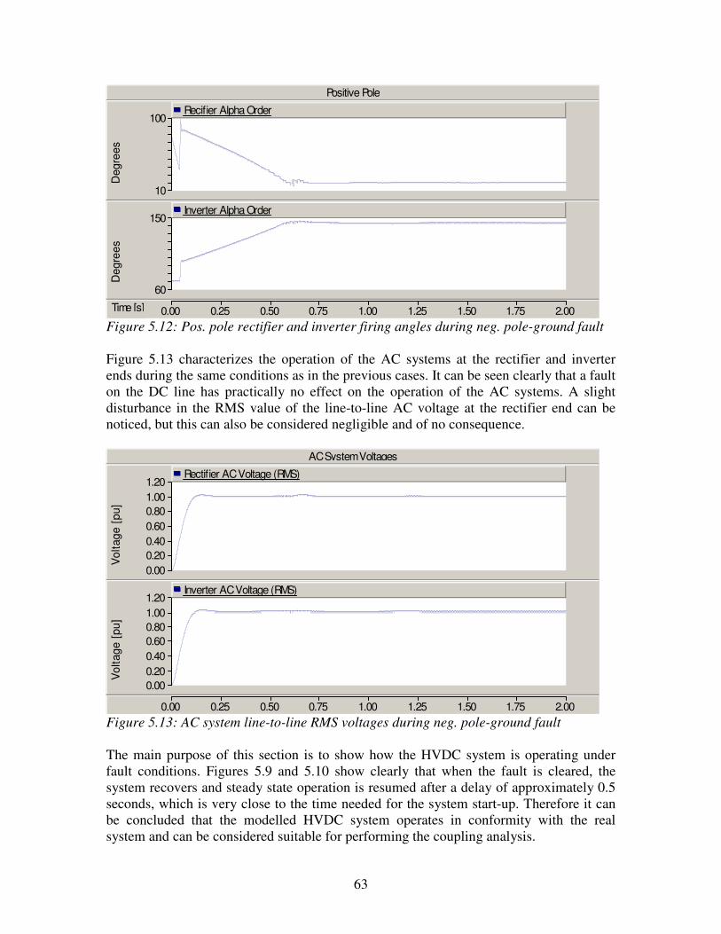
63

Positive Pole

Time [s] 0.00 0.25 0.50 0.75 1.00 1.25 1.50 1.75 2.00 ... ...

10

100 D

egre

esRecifier Alpha Order

60

150

Deg

rees

Inverter Alpha Order

Figure 5.12: Pos. pole rectifier and inverter firing angles during neg. pole-ground fault Figure 5.13 characterizes the operation of the AC systems at the rectifier and inverter ends during the same conditions as in the previous cases. It can be seen clearly that a fault on the DC line has practically no effect on the operation of the AC systems. A slight disturbance in the RMS value of the line-to-line AC voltage at the rectifier end can be noticed, but this can also be considered negligible and of no consequence.

AC System Voltages

0.00 0.25 0.50 0.75 1.00 1.25 1.50 1.75 2.00 ... ...

0.00 0.20 0.40 0.60 0.80 1.00 1.20

Rectifier AC Voltage (RMS)

Vol

tage

[pu

]

0.00 0.20 0.40 0.60 0.80 1.00 1.20

Vol

tage

[pu

]

Inverter AC Voltage (RMS)

Figure 5.13: AC system line-to-line RMS voltages during neg. pole-ground fault The main purpose of this section is to show how the HVDC system is operating under fault conditions. Figures 5.9 and 5.10 show clearly that when the fault is cleared, the system recovers and steady state operation is resumed after a delay of approximately 0.5 seconds, which is very close to the time needed for the system start-up. Therefore it can be concluded that the modelled HVDC system operates in conformity with the real system and can be considered suitable for performing the coupling analysis.

64

5.2. Coupling Phenomenon – Basecase PSCAD coupling phenomenon analysis and results constitute the subject of Sections 5.2 to 5.4 of this report. In the present section this subject is presented in reference to the results obtained for the so called basecase system. The basecase system is shown in Figure 5.14 and selected key parameters used are given in Table 5.1 below. Wherever available, parameters used in the basecase model correspond to design parameters of the real system. As already mentioned the coupling phenomenon was studied considering a line-to-ground fault on the negative pole of the HVDC system for the two coupled sections, namely:

1. Coupled Section 1 : RoW consisting of the HVDC negative pole overhead line section and the 400kV AC line,

2. Coupled Section 2: RoW consisting of the HVDC negative pole overhead line section and the 220kV AC line.

The two coupled sections are clearly marked in Figure 5.14 and their details are provided in Table 5.1. To make the discussion easier to follow, in the absence of the actual substation names, the terminating substations for the 400kV and 220kV AC transmission lines have been give hypothetical names. As can be noted from Figure 5.14, the terminating substations for the 400kV AC line have been called Substation 400A (Forsmark substation) and Substation 400B, and similarly, those for the 220kV AC line have been called Substation 220A and Substation 220B. For the basecase, coupling has been studied for a fault at point B (Fault B) of the negative pole, since this point gives the highest coupling for the 400kV case, and for a fault at point A (Fault A) of the negative pole, as this fault results in the highest coupling for the 220kV line. In Section 5.3, a parametric or sensitivity analysis of the coupling phenomenon is presented.

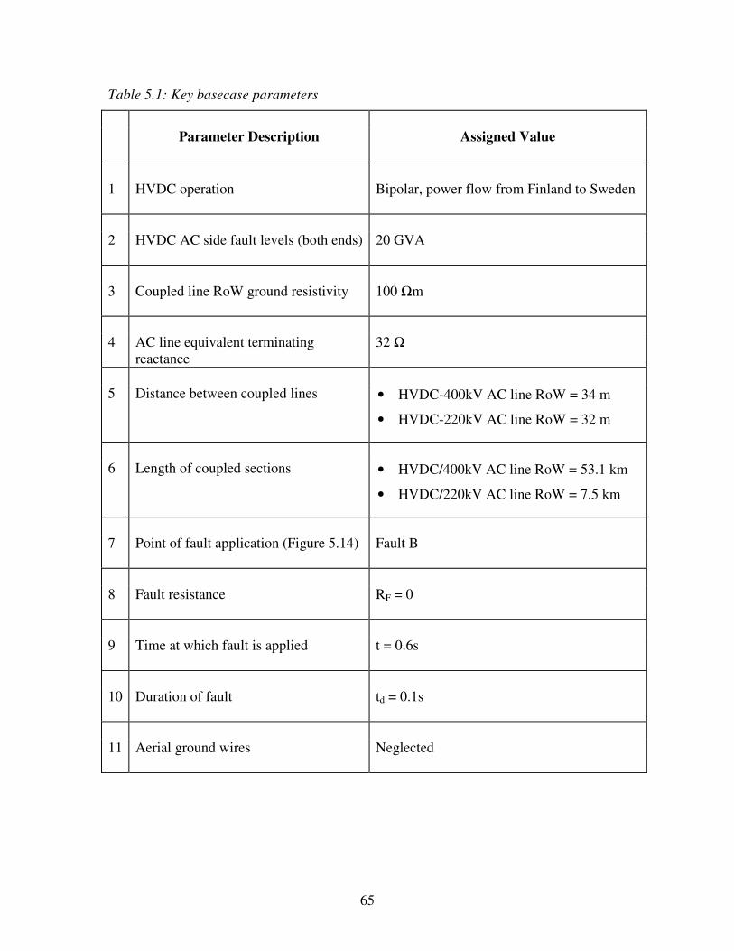
65

Table 5.1: Key basecase parameters

Parameter Description Assigned Value

1 HVDC operation Bipolar, power flow from Finland to Sweden

2 HVDC AC side fault levels (both ends) 20 GVA

3 Coupled line RoW ground resistivity 100 m

4 AC line equivalent terminating reactance

32

5 Distance between coupled lines • HVDC-400kV AC line RoW = 34 m

• HVDC-220kV AC line RoW = 32 m

6 Length of coupled sections • HVDC/400kV AC line RoW = 53.1 km

• HVDC/220kV AC line RoW = 7.5 km

7 Point of fault application (Figure 5.14) Fault B

8 Fault resistance RF = 0

9 Time at which fault is applied t = 0.6s

10 Duration of fault td = 0.1s

11 Aerial ground wires Neglected

66

Figure 5.14: Drawing for coupling studies

MVA

MVA

67

5.2.1. Coupled Section 1: RoW Consisting of the HVDC Negative Pole Overhead Line Section and the 400kV AC Line Coupling results in relation to the 400kV AC line are discussed in this section for the following cases

i. Normal operation ii. Line-to-ground fault on the negative pole

5.2.1.1. Coupling During Normal Operation We begin our presentation of results for the basecase considering normal operation of the HVDC system. Under this condition virtually no coupling exists between the HVDC and the 400kV AC line. The results obtained are shown in Figure 5.15 below with measurements taken at Substation 400A.

Substation 400A

Time [s] 0.00 0.25 0.50 0.75 1.00 1.25 1.50 1.75 2.00 ... ...

-0.1000

0.1000

Cur

rent

[kA

]

<Neutral Current >

0.0

0.1000

Cur

rent

[kA

]

<Neutral Current RMS>

0.0

0.0100

Cur

rent

[kA

]

<Neutral Current Fundamental RMS>

Figure 5.15: Total coupled current under normal operation The non-zero values (though still negligible) obtained for slightly more than 0.5s in Figure 5.15 can be attributed to HVDC system start-up which process occurs transiently. The current shown in Figure 5.15 is the neutral current which is the sum of the phase currents. Plots of coupled phase currents, though not shown here, are of no interest due to the fact that they are also of zero magnitude under normal operation of the HVDC.

68

5.2.1.2. Coupling During Line-to-Ground Fault on the Negative Pole A line-to-ground fault was applied at fault point B in Figure 5.14. Fault point B is of great interest because, as will be seen in the sensitivity analysis, it results in the highest coupling into the 400kV AC line. With this fault applied, results are presented for the following:

i. Analysis of contributions to the fault current ii. Coupled currents in the 400kV line including neutral and phase quantities

iii. Coupled voltages in the 400kV line including neutral and phase quantities iv. Neutral current sequence component and harmonic analysis

(i) Fault Current Contributions Figure 5.16 below shows the contributions to the fault current from the HVDC system and from the undersea DC cable. It can be observed that while the HVDC system limits the fault current through the rectifier to about 2.8 p.u. (fault current of 4.5kA at nominal current of 1.6kA), a large fraction of the fault current that follows to the ground is due to the discharging of the DC cable.

Contribution to the Fault Current

Time [s] 0.50 0.60 0.70 0.80 0.90 1.00 1.10 1.20 ... ...

-10.0 -5.0 0.0 5.0

10.0 15.0

Cur

rent

[kA

]

<DC Cable Discharging Current>

0.0

4.50

Cur

rent

[kA

]

<Negative Pole Rectifier DC Current>

-7.5

17.5

Cur

rent

[kA

]

<Total Fault Current From Ground Sources>

Figure 5.16: Contributions to the fault current

69

(ii) Coupled Currents in the 400kV Line Figures 5.17 and 5.18 show the coupled currents in the 400kV line at Substation 400A and Substation 400B respectively. The currents were measured flowing into the line at both substations and it can be observed that the currents at the two substations are equal in magnitude, but in anti-phase with each other. Since the 400kV line is of a short-line type (72km), it is not a surprising result that the currents at the two ends of the line are of equal magnitude. It can also be observed that the induced current has the same shape as that of the fault current. In Figures 5.17 and 5.18, it can be noted that the total induced current peaks at about 2kA with an RMS peak of about 1.2kA. Of the total RMS current, about 58% (700A) is due to the fundamental current and the rest is contributions from the other harmonics as will be shown under harmonic analysis. This clearly shows that the coupled current during this fault type is significant and evaluation of its impact on the protection of the AC line is a worth undertaking. It is also noted that the coupled current is transient in nature and decays to zero in about 60ms.

Substation 400A

Time [s] 0.500 0.550 0.600 0.650 0.700 0.750 0.800 ... ...

-0.50 0.00 0.50 1.00 1.50 2.00 2.50

Cur

rent

[kA

]

<Neutral Current >

0.00 0.20 0.40 0.60 0.80 1.00 1.20

Cur

rent

[kA

]

<Neutral Current RMS>

0.0

0.70

Cur

rent

[kA

]

<Neutral Current Fundamental RMS>

Figure 5.17: Substation 400A, 400kV line coupled current under fault condition

70

Substation 400B

Time [s] 0.500 0.550 0.600 0.650 0.700 0.750 0.800 ... ...

-2.50 -2.00 -1.50 -1.00 -0.50 0.00 0.50

Cur

rent

[kA

]<Neutral Current >

0.00 0.20 0.40 0.60 0.80 1.00 1.20

Cur

rent

[kA

]

<Neutral Current RMS>

0.0

0.70

Cur

rent

[kA

]

<Neutral Current Fundamental RMS>

Figure 5.18: Substation 400B, 400kV line coupled current under fault condition

In Figures 5.19 and 5.20, respective phase currents induced at Substation 400A and Substation 400B are shown. Like the total coupled current, the coupled currents in the phases are equal at the two substations. Furthermore, these phase currents are identical in all phases.

Substation 400A

Time [s] 0.500 0.550 0.600 0.650 0.700 0.750 0.800 ... ...

-0.10

0.70

Cur

rent

[kA

]

<Phase A Current>

-0.10

0.70

Cur

rent

[kA

]

<Phase B Current>

-0.10

0.70

Cur

rent

[kA

]

<Phase C Current>

Figure 5.19: Substation 400A, 400kV line coupled phase currents under fault condition

71

Substation 400B

Time [s] 0.500 0.550 0.600 0.650 0.700 0.750 0.800 ... ...

-0.70

0.10 C

urre

nt [

kA]

<Phase A Current>

-0.70

0.10

Cur

rent

[kA

]

<Phase B Current>

-0.70

0.10

Cur

rent

[kA

]

<Phase C Current>

Figure 5.20: Substation 400B, 400kV line coupled phase currents under fault condition

(iii) Coupled voltages in the 400kV Line The coupled phase-to-ground voltages, measured at substations 400A and 400B, are shown in Figures 5.21 and 5.22 respectively.

Substation 400A

Time [s] 0.500 0.550 0.600 0.650 0.700 0.750 0.800 ... ...

-30 -20 -10

0 10 20

Vol

tage

[kV

]

<Phase A Voltage>

-30 -20 -10

0 10 20

Vol

tage

[kV

]

<Phase B Voltage>

-30 -20 -10

0 10 20

Vol

tage

[kV

]

<Phase C Voltage>

Figure 5.21: Substation 400A, 400kV line coupled phase voltages under fault condition

72

Substation 400B

Time [s] 0.500 0.550 0.600 0.650 0.700 0.750 0.800 ... ...

-25.0

20.0 V

olta

ge [

kV]

<Phase A Voltage>

-25.0

20.0

Vol

tage

[kV

]

<Phase B Voltage>

-25.0

20.0

Vol

tage

[kV

]

<Phase C Voltage>

Figure 5.22: Substation 400B, 400kV line coupled phase voltages under fault condition The explanation relating to the coupled phase currents equally applies to the coupled phase voltages, except that due to the difference in distances from the coupled section to the two substations at the ends of the line, the induced phase-to-ground voltages at the two substations are not equal. At Substation 400A the peak value of the phase voltages is about 30kV compared to 25kV for those induced at Substation 400B.

(iv) Sequence Component & Harmonic Analysis To understand the sequence component composition of the coupled currents, a sequence component analysis was carried out. Since it has already been shown that coupled currents at the two ends of the line are equal, this analysis was only done for Substation 400A. In Figure 5.23 below, results clearly demonstrate that positive and negative sequence currents are negligible or totally absent from the coupled currents. On the contrary, a look at Figure 5.24 shows that the coupled currents are about 100% zero sequence currents. In the figure the first 5 harmonics of the zero sequence currents are presented. As would be expected, the fundamental current has the highest magnitude, followed by the second, third, fourth and fifth in that order. The observation here that coupling is far more stronger between zero sequence networks, when compared to positive and negative sequence networks, agrees well with what can be found in literature [15]. This fact will be useful in explaining the role of ground

73

resistivity in the coupling phenomenon as one of the parametric analyses presented under sensitivities in Section 5.3.

Substation 400A

Time [s] 0.500 0.550 0.600 0.650 0.700 0.750 0.800 ... ...

-0.100

0.100

Cur

rent

[kA

]

<Pos. Sequence Current RMS>

-0.100

0.100

Cur

rent

[kA

]

<Neg. Sequence Current RMS>

Figure 5.23: Positive & negative sequence components present in coupled currents

Substation 400A: Zero Sequence Current Harmonics (first 5)

Time [s] 0.590 0.600 0.610 0.620 0.630 0.640 0.650 0.660 0.670 0.680 ... ...

0.000

0.025

0.050

0.075

0.100

0.125

0.150

0.175

0.200

0.225

Cur

rent

[kA

]

<1st> <2nd> <3rd> <4th> <5th>

Figure 5.24: Zero sequence components present in coupled currents

74

Substation 400A

Time [s] 0.00 0.25 0.50 0.75 1.00 1.25 1.50 1.75 2.00 ... ...

-0.100

0.100 V

olta

ge [

kV]

<Pos. Sequence Voltage RMS>

-0.100

0.100

Vol

tage

[kV

]

<Neg. Sequence Voltage RMS>

Figure 5.25: Positive & negative sequence components present in coupled voltages The behaviour observed in sequence currents is well replicated in sequence voltages. Figure 5.25 shows a clear absence of positive and negative sequence voltages, whereas Figure 5.26 demonstrates a full presence of zero sequence voltages, suggesting a very strong coupling in the zero-sequence networks.

Substation 400A: Zero Sequence Voltage Harmonics (first 5)

Time [s] 0.590 0.600 0.610 0.620 0.630 0.640 0.650 0.660 0.670 0.680 ... ...

0.0

1.0

2.0

3.0

4.0

5.0

6.0

7.0

8.0

9.0

Vol

tage

[kV

]

<1st> <2nd> <3rd> <4th> <5th>

Figure 5.26: Zero-sequence components present in coupled voltages Harmonic analysis of the total coupled current (neutral current) yields a spectrum of frequencies that are present in the coupled quantities. The first 5 harmonics are plotted in Figure 5.27 below. The spectrum pattern fully resembles that obtained for zero sequence currents in Figure 5.24, though here the magnitudes have increased three-fold, since the currents considered are total currents. The pattern is repeated where the first and second harmonics are much higher in comparison to the higher harmonics. The harmonic magnitude decreases when moving from lower to higher harmonic orders.

75

Substation 400A: Neutral Current Harmonics (first 5)

Time [s] 0.590 0.600 0.610 0.620 0.630 0.640 0.650 0.660 0.670 0.680 ... ...

0.00

0.10

0.20

0.30

0.40

0.50

0.60

0.70 C

urre

nt [

kA]

<1st> <2nd> <3rd> <4th> <5th>

Figure 5.27: Harmonic spectrum of the total coupled current

5.2.2. Coupled Section 2: RoW Consisting of the HVDC Negative Pole Overhead Line Section and the 220kV AC Line This section treats the fault on the negative pole, which gives the highest coupling in the 220kV overhead AC line. A line-to-ground fault was applied at the fault point A in Figure 5.14. This position gives the highest coupling in the 220kV AC line. With this fault applied, results are presented for the following:

i. Coupled currents in the 220kV line including neutral and phase quantities ii. Coupled voltages in the 220kV line including neutral and phase quantities

iii. Total coupled current (neutral current) sequence component and harmonic analysis

(i) Coupled Currents in the 220kV Line

In figures 5.28 and 5.29, it can be noted that the worst fault results in the total induced current in the 220kV line with a peak of about 600A. This is much less when compared to 2000A obtained for the 400kV line. In RMS terms, this current has a peak slightly less than 400A of which about 70% is due to the fundamental current. In comparison to the 400kV line, the coupled current in the 220kV line is much lower. This can be explained on account of the differences in lengths between the two coupled sections of the two lines; 7.5km for the 220kV line compared to 53.1 for the 400kV line. Though the coupling in the 220kV line is not as significant as for the 400kV line, the current behaviour is however very much similar to the 400kV case - the coupled current is of transient nature and decays to zero in about 60ms.

76

Substation 220A

Time [s] 0.500 0.550 0.600 0.650 0.700 0.750 0.800 ... ...

-0.20

0.60 C

urre

nt [

kA]

<Neutral Current>

0.0

0.400

Cur

rent

[kA

]

<Neutral Current RMS>

0.000 0.050 0.100 0.150 0.200 0.250 0.300

Cur

rent

[kA

]

<Neutral Current Fundamental RMS>

Figure 5.28: Substation 220A, 220kV line coupled current under fault condition

Substation 220B

Time [s] 0.500 0.550 0.600 0.650 0.700 0.750 0.800 ... ...

-0.60

0.20

Cur

rent

[kA

]

<Neutral Current>

0.0

0.400

Cur

rent

[kA

]

<Neutral Current RMS>

0.000 0.050 0.100 0.150 0.200 0.250 0.300

Cur

rent

[kA

]

<Neutral Current Fundamental RMS>

Figure 5.29: Substation 220B, 220kV line coupled current under fault condition

77

Figures 5.30 and 5.31 characterise respective phase currents induced at Substation 220A and Substation 220B. Like the total coupled current, the coupled currents in the phases are equal at the two substations. The phase currents are also identical in all phases.

Substation 220A

Time [s] 0.500 0.550 0.600 0.650 0.700 0.750 ... ...

-0.100 -0.050 0.000 0.050 0.100 0.150 0.200

Cur

rent

[kA

]

<Phase A Current>

-0.100 -0.050 0.000 0.050 0.100 0.150 0.200

Cur

rent

[kA

]

<Phase B Current>

-0.100 -0.050 0.000 0.050 0.100 0.150 0.200

Cur

rent

[kA

]

<Phase C Current>

Figure 5.30: Substation 220A, 220kV line coupled phase currents under fault condition

Substation 220B

Time [s] 0.500 0.550 0.600 0.650 0.700 0.750 0.800 ... ...

-0.200 -0.150 -0.100 -0.050 0.000 0.050

Cur

rent

[kA

]

<Phase A Current>

-0.200 -0.150 -0.100 -0.050 0.000 0.050

Cur

rent

[kA

]

<Phase B Current>

-0.200 -0.150 -0.100 -0.050 0.000 0.050

Cur

rent

[kA

]

<Phase C Current>

Figure 5.31: Substation 220B, 220kV line coupled phase currents under fault condition

78

(ii) Coupled Voltages in the 220kV Line Figures 5.32 and 5.33 are plots of the phase voltages at Substation 220A and Substation 220B respectively. The explanation above, relating to the coupled phase currents, equally applies to the coupled phase voltages at the two substations, except that due to the difference in distances from the coupled section to the two substations at the ends of the line, the induced phase-to-ground voltages at the two substations are not equal.

Substation 220A

Time [s] 0.500 0.550 0.600 0.650 0.700 0.750 0.800 ... ...

-12.0

8.0

Vol

tage

[kV

]

<Phase A Voltage>

-12.0

8.0

Vol

tage

[kV

]

<Phase B Voltage>

-12.0

8.0

Vol

tage

[kV

]

<Phase C Voltage>

Figure 5.32: Substation 220A, 220kV line coupled phase voltages under fault condition 220 kV substation B

79

Substation 220B

Time [s] 0.500 0.550 0.600 0.650 0.700 0.750 0.800 ... ...

-6.0

5.0 V

olta

ge [

kV]

<Phase A Voltage>

-6.0

5.0

Vol

tage

[kV

]

<Phase B Voltage>

-6.0

5.0

Vol

tage

[kV

]

<Phase C Voltage>

Figure 5.33: Substation 220B, 220kV line coupled phase voltages under fault condition

(iii) Sequence Component & Harmonic Analysis Figure 5.34 and 5.35 below characterise the zero-sequence components of the coupled currents and voltages respectively. Both positive and negative sequence components are either negligible or totally absent from the coupled quantities. In the figure, the first 5 harmonics of the zero sequence currents are presented. As would be expected, the fundamental current has the highest magnitude, followed by the second, third, fourth and fifth in that order for both current and voltage.

Substation 220A: Zero Sequence Current Harmonics (first 5)

Time [s] 0.590 0.600 0.610 0.620 0.630 0.640 0.650 0.660 0.670 0.680 ... ...

0.000

0.010

0.020

0.030

0.040

0.050

0.060

0.070

0.080

0.090

Cur

rent

[kA

]

<1st> <2nd> <3rd> <4th> <5th>

Figure 5.34: Zero-sequence components present in the coupled currents

80

Substation 220A: Zero Sequence Voltage Harmonics (first 5)

Time [s] 0.590 0.600 0.610 0.620 0.630 0.640 0.650 0.660 0.670 0.680 ... ...

0.00

0.50

1.00

1.50

2.00

2.50

3.00 V

olta

ge [

kV]

<1st> <2nd> <3rd> <4th> <5th>

Figure 5.35: Zero-sequence components present in the coupled voltages Harmonic analysis of the total coupled current (neutral current) yields a spectrum of frequencies that are present in the coupled quantities. The first 5 harmonics are plotted in Figure 5.36 below. The pattern obtained here is very similar to the 400kV case except for the magnitudes, which, as expected, are much lower.

Substation 220A: Neutral Current Harmonics (first 5)

Time [s] 0.590 0.600 0.610 0.620 0.630 0.640 0.650 0.660 0.670 0.680 ... ...

0.000

0.050

0.100

0.150

0.200

0.250

0.300

Cur

rent

[kA

]

<1st> <2nd> <3rd> <4th> <5th>

Figure 5.36: Harmonic spectrum of the total coupled current

81

5.3. Sensitivity Analysis The aim of this section is to show how coupled currents are affected by varying a number of selected parameters. The parametric studies are presented considering a wide range of parameters. Parameters investigated include:

(i) Fault position on the HVDC negative pole (ii) Soil resistivity

(iii) Distance between coupled lines (iv) Length of the coupled section (v) Value of equivalent line terminating impedance

(vi) Fault resistance (vii) Inclusion of aerial ground wires

(viii) Effect of AC system short circuit levels Parametric analysis was carried out for the coupled section involving the 400kV line only (coupled section 1) since, as shown in Section 5.2, this is the coupled section that gives significant coupling to the AC line. Parameters were varied one at a time, i.e. other parameters were kept the same as in the basecase. The effect of changing various parameters was monitored only at Substation 400A (Forsmark) because the measured values differ only negligibly from those measured at Substation 400B.

5.3.1. Effect of Fault Position The position of fault application was moved along the negative pole of the HVDC link and variations in the coupled currents to the 400kV line were monitored. The fault application positions are shown in Figure 5.14 and are as follows:

1. Fault A – fault at the inverter (Swedish) end after the smoothing reactor, 2. Fault B – fault at the beginning of the coupled section 1, 3. Fault C – fault in the middle of the coupled section 1 (26,55 km from Fault B), 4. Fault D – fault at the end of the coupled section 1 (53,1 km from Fault B), and 5. Fault E – fault at the rectifier (Finnish) end before the smoothing reactor.

Observed variations in coupled currents due to fault position change are shown in Figures 5.37 and 5.38 for the total current and total RMS current respectively. Two observations can be made from these plots:

a) The fault position that results in the highest current through the coupled section gives the highest coupling, and

b) Coupling is highest for a fault position which results in a fault current that flows

in the entire length of the coupled section – this seems reasonable as this would result in the highest flux linkage.

82

In Figures 5.37 and 5.38 fault B gives the highest coupling since it satisfies both (a) and (b) above, followed by fault A and then C. Coupling due to fault D and E is negligible since these fault positions hardly meet requirements (a) and (b) stated above.

Substation 400A: Neutral RMS Current vs Fault Position

Time [s] 0.600 0.620 0.640 0.660 0.680 0.700 ... ...

0.00

0.20

0.40

0.60

0.80

1.00

1.20

Cur

rent

[kA

]

<Fault A> <Fault B> <Fault C> <Fault D> <Fault E>

Figure 5.37: Variation of total RMS coupled currents with HVDC fault position

Substation 400A: Neutral RMS Fundamental Current vs Fault Position

Time [s] 0.600 0.620 0.640 0.660 0.680 0.700 ... ...

0.00

0.10

0.20

0.30

0.40

0.50

0.60

0.70

Cur

rent

[kA

]

<Fault A> <Fault B> <Fault C> <Fault D> <Fault E>

Figure 5.38: Variation of fundamental RMS coupled currents with HVDC fault position

83

5.3.2. Effect of Soil Resistivity In Section 5.2, it was shown that coupling during line-to-ground fault was almost entirely due to zero-sequence transients. The consequence of this is that soil resistivity becomes a key parameter in the determination of whether there will be coupling or not. In Figures 5.39 and 5.40, it can be observed that for any value of soil resistivity other than zero, the coupled current in the 400kV line is significant and with about the same order of magnitude. For zero soil resistivity the coupled current is negligible. This observation can also be found in literature [5].

Substation 400A: Neutral RMS Current vs Soil Resisivity

Time [s] 0.600 0.620 0.640 0.660 0.680 0.700 ... ...

0.00

0.20

0.40

0.60

0.80

1.00

1.20

Cur

rent

[kA

]

<0 ohm-m> <10 ohm-m> <100 ohm-m> <500 ohm-m> <1000 ohm-m>

Figure 5.39: Variation of total RMS coupled currents with soil resistivity

84

Substation 400A: Neutral RMS Fundamental Current vs Soil Resistivity

Time [s] 0.600 0.620 0.640 0.660 0.680 0.700 ... ...

0.00

0.10

0.20

0.30

0.40

0.50

0.60

0.70

Cur

rent

[kA

]<0 ohm-m> <10 ohm-m> <100 ohm-m> <500 ohm-m> <1000 ohm-m>

Figure 5.40: Variation of fundamental RMS coupled currents with soil resistivity

5.3.3. Effect of Distance Between Coupled Lines Figure 5.40 and 5.41 present, respectively, the coupled total and fundamental RMS currents in the AC line with respect to different interline distances between the Dannebo-Finnböle HVDC line and the 400 kV AC line.

Substation 400A: Neutral RMS Current vs Interline Distance

Time [s] 0.600 0.620 0.640 0.660 0.680 0.700 ... ...

0.00

0.20

0.40

0.60

0.80

1.00

1.20

Cur

rent

[kA

]

<26 m> <34 m> <50 m> <100 m> <1000 m>

Figure 5.40: Variation of total RMS coupled currents with interline distance

85

Substation 400A: Neutral RMS Fundamental Current vs Interline Distance

Time [s] 0.600 0.620 0.640 0.660 0.680 0.700 ... ...

0.00

0.10

0.20

0.30

0.40

0.50

0.60

0.70

0.80

Cur

rent

[kA

]<26 m> <34 m> <50 m> <100 m> <1000 m>

Figure 5.41: Variation of fundamental RMS coupled currents with interline distance It can be seen from Figures 5.40 and 5.41 that the effect of interline distance can be considered almost linear for both, the total and the fundamental RMS currents. The highest coupling occurs for the closest interline distance (26m between the tower centres), whereas the lowest coupling is caused by the farthest distance between the lines (1000m).

5.3.4. Effect of Coupled Section Length In this parametric study we show the effect of varying the length of the coupled section on the coupled currents. The results are plotted in Figures 5.42 and 5.43 for the total coupled current and the fundamental current respectively. The key observation here is that while, as expected, the coupled current increases with the length of the coupled section, the relationship has a maximum after which any increase in the length of the coupled section results in decreased coupled currents. For instance in Figures 5.43 the coupled fundamental current is higher for a coupled section length of 150km compared to that of 500km. It would appear as the length increases beyond a certain point the line self-impedance matrix increases to the extent that it begins to decrease the coupled currents.

86

Substation 400A: Neutral RMS Current vs Coupled Section Length

Time [s] 0.600 0.620 0.640 0.660 0.680 0.700 ... ...

0.00

0.25

0.50

0.75

1.00

1.25

1.50

1.75

2.00

2.25 C

urre

nt [

kA]

<25 km> <53 km> <150 km> <500 km> <1000 km>

Figure 5.42: Variation of total RMS coupled currents with length of the coupled section

Substation 400A: Neutral RMS Fundamental Current vs Coupled Section Length

Time [s] 0.600 0.620 0.640 0.660 0.680 0.700 ... ...

0.00

0.20

0.40

0.60

0.80

1.00

1.20

Cur

rent

[kA

]

<25 km> <53 km> <150 km> <500 km> <1000 km>

Figure 5.43: Variation of fundamental RMS coupled currents RMS with length of the

coupled section

87

5.3.5. Effect of Equivalent Terminating Impedance The effect of varying the equivalent line terminating impedances for the coupled total and fundamental RMS currents is given by Figures 5.44 and 5.45 respectively. The equivalent impedance means the impedance of all the zero sequence sources that are in parallel at the line terminating substations. For simplicity, the resistance was neglected since it is much smaller than the inductance of the line terminating transformers.

Substation 400A: Neutral RMS Current vs Equivalent Line Terminating Impedance

Time [s] 0.600 0.620 0.640 0.660 0.680 0.700 ... ...

0.00

0.20

0.40

0.60

0.80

1.00

1.20

1.40

1.60

Cur

rent

[kA

]

<16 ohm> <32 ohm> <80 ohm> <112 ohm> <160 ohm>

Figure 5.44: Total RMS coupled currents versus equivalent terminating impedance

Substation 400A: Neutral RMS Fundamental Current vs Equivalent Line Terminating Impedance

Time [s] 0.600 0.620 0.640 0.660 0.680 0.700 ... ...

0.00

0.10

0.20

0.30

0.40

0.50

0.60

0.70

0.80

0.90

1.00

Cur

rent

[kA

]

<16 ohm> <32 ohm> <80 ohm> <112 ohm> <160 ohm>

Figure 5.45: Fundamental RMS coupled currents vs equivalent terminating impedance

88

From Figures 5.44 and 5.45 it is easy to see that the effect can again be considered closely to linear. The highest coupling is caused by the lowest equivalent impedance and the lowest coupling by the highest impedance.

5.3.6. Effect of fault resistance Figures 5.46 and 5.47 represent the effect of the negative pole-to-ground fault arc resistance on the coupled current in the 400 kV AC line

Substation 400A: Neutral RMS Current vs Fault Resistance

Time [s] 0.600 0.620 0.640 0.660 0.680 0.700 ... ...

0.00

0.20

0.40

0.60

0.80

1.00

1.20

Cur

rent

[kA

]

<R=0 ohm> <R=5 ohm> <R=25 ohm> <R=50 ohm> <R=100 ohm>

Figure 5.46: Total RMS coupled currents versus fault resistance

Substation 400A: Neutral RMS Fundamental Current vs Fault Resistance

Time [s] 0.600 0.620 0.640 0.660 0.680 0.700 ... ...

0.00

0.10

0.20

0.30

0.40

0.50

0.60

0.70

Cur

rent

[kA

]

<R=0 ohm> <R=5 ohm> <R=25 ohm> <R=50 ohm> <R=100 ohm>

Figure 5.47: Fundamental RMS coupled currents versus fault resistance

89

Again, almost linear relationships for the total and fundamental coupled currents can be obtained from Figures 5.46 and 5.47. In the basecase the simulations were done with bolted pole-to-ground fault (R=0), which means that in reality smaller values of coupled currents to the 400kV AC line are expected.

5.3.7. Effect of Aerial Ground Wires In the base case the transmission lines were modelled without aerial ground wires for simplicity. To understand whether ground wires have any effect on the coupled currents, a parametric analysis was carried out with ground wires included. The results obtained are shown in Figures 5.48 and 5.49 for line-to-ground faults applied at fault positions A and fault positions B respectively. With a fault at fault position A, the obtained coupled currents in the cases with or without ground wires are equal. For the case with a fault applied at fault point B, there is a small mismatch between coupled currents for the two cases. The with-ground-wire case shows a slightly higher coupled current in comparison to the without-ground-wire case (Figure 5.49). Fault A and Fault B were found to be the lower and upper limiting cases, i.e. fault position A gave no mismatch in the coupled currents between the with-ground-wire case and the without-ground-wire case, while fault point B gave the largest mismatch. Considering that even with a fault position giving the largest coupled current mismatch the difference is for all practical purposes negligible, it can be concluded that the aerial ground wires have no or little effect on the coupling phenomenon.

Substation 400A: Neutral RMS Current

Time [s] 0.600 0.620 0.640 0.660 0.680 0.700 ... ...

0.00

0.20

0.40

0.60

0.80

1.00

Cur

rent

[kA

]

<With Ground Wires> <Without Ground Wires>

Figure 5.48: Effect of aerial ground wires on coupled currents (Fault A)

90

Substation 400A: Neutral RMS Current

Time [s] 0.600 0.620 0.640 0.660 0.680 0.700 ... ...

0.00

0.20

0.40

0.60

0.80

1.00

1.20

Cur

rent

[kA

]<With Ground Wires> <Without Ground Wires>

Figure 5.49: Effect of aerial ground wires on coupled currents (Fault B)

5.3.8. Effect of AC System Short Circuit Levels Figure 5.50 compares the total coupled RMS neutral current in the 400 kV AC line between two different values of the rectifier (Finnish) AC system short circuit levels – 3 GVA and 50 GVA. The result obtained from the simulations is somewhat unexpected, because it was always assumed that the rectifier AC system short circuit level had a remarkable effect on the DC system fault current and thus, on the coupled current to the AC system. But, even by changing the short circuit level very much, from 3 GVA to 50 GVA in this case, no remarkable change in the coupled current to the AC system was obtained from the simulations. The same pattern also applies when the short circuit level of the inverter end AC system is varied. Therefore, it can be concluded that the mutual coupling between overhead DC lines and AC lines is not dependant on the AC system strengths at the ends of a DC link.

91

Substation 400A: Neutral RMS Current vs Rectifier (Finnish) AC System Short Circuit Level

Time [s] 0.600 0.620 0.640 0.660 0.680 0.700 ... ...

0.00

0.20

0.40

0.60

0.80

1.00

1.20 C

urre

nt [

kA]

<3 GVA> <50 GVA>

Figure 5.50: Variation of the total RMS coupled currents with changing the rectifier (Finnish) AC system short circuit level

92

5.4. Coupling Phenomenon with Monopolar Operation To determine the amount of induced currents during monopolar operation, the positive pole converters were taken out of service and the negative pole then used the positive pole conductor as a return path. The worst fault condition (Fault B) was simulated and the results obtained are plotted in Figure 5.51. A comparison of Figure 5.51 and Figure 5.17 obtained for the basecase shows that changing the mode of operation from bipolar to monopolar has no effect on the coupled current. The same results were also obtained when the monopolar operation was changed from metallic return to ground return.

Substation 400A

Time [s] 0.560 0.580 0.600 0.620 0.640 0.660 0.680 0.700 ... ...

-0.50 0.00 0.50 1.00 1.50 2.00 2.50

Cur

rent

[kA

]

<Neutral Current >

0.00 0.20 0.40 0.60 0.80 1.00 1.20

Cur

rent

[kA

]

<Neutral Current RMS>

0.0

0.70

Cur

rent

[kA

]

<Neutral Current Fundamental RMS>

Figure 5.51: Total coupled currents during monopolar operation

93

5.5. Coupling Phenomenon with Reverse Power Operation The study carried out in this section has the objective of determining whether a reversal in the power flow direction, from that used in the basecase study (Finland to Sweden), to one, where power flows from Sweden to Finland in the HVDC system, would have any impact on the coupled current. The study was done for the most onerous fault position (Fault B). The results obtained are shown in Figure 5.52. Comparing this plot with the one obtained for the base case (Figure 5.17) shows that under reverse power operation the coupled current obtained has the same magnitude as in the base case. However, the coupled current direction during the fault is reversed on account of the reversal of the power flow direction in the HVDC.

Substation 400A

Time [s] 0.560 0.580 0.600 0.620 0.640 0.660 0.680 0.700 ...

-2.50

1.00

Cur

rent

[kA

]

<Neutral Current >

0.00 0.20 0.40 0.60 0.80 1.00 1.20

Cur

rent

[kA

]

<Neutral Current RMS>

0.0

0.80

Cur

rent

[kA

]

<Neutral Current Fundamental RMS>

Figure 5.52: Total coupled currents during HVDC reverse power operation

94

6. MATLAB MODEL AND RESULTS In addition to the PSCAD simulations presented in the foregoing two chapters, a MATLAB program was developed to confirm the existence of coupled currents in the HVAC lines due to a pole-to-ground fault in the HVDC system. The MATLAB model and results obtained therefrom are the subject of discussion of this chapter. The MATLAB code was developed based on the coupling phenomenon conceptualisation and equations developed and discussed in Section 2.5 of this report. In comparison to the PSCAD simulation, in which results were obtained in absolute terms, it will be observed that the results obtained from the MATLAB model are rather conceptual. However, efforts have been made to demostrate agreement between MATLAB and PSCAD results. 6.1. MATLAB Model As stated in various articles [11,12,14] and confirmed by the PSCAD simulations (Section 5.2), the most significant coupling occurs between the zero-sequence networks of the two lines. The coupling between the positive and negative sequence networks is marginal and can therefore be neglected. Thus, it was decided to model only the zero-sequence networks of the 500kV Dannebo-Finnböle HVDC line and the parallel 400kV HVAC line in MATLAB; the positive and negative sequences were not considered. The concept of the coupling analysis is given by Figure 6.1 and it is similar to that of [14]; the AC line was terminated with equivalent zero sequence impedances at both line ends (nodes 2 and 4) and the DC line was terminated by the converter transformer zero-sequence impedance (node 3).

Figure 6.1: Zero-sequence networks of the coupled AC and DC lines modelled in

MATLAB The study of coupling was performed in MATLAB by the same principle as given in Section 2.5 of this report. First, the code for calculating the zero-sequence ABCD and admittance matrices of the coupled lines was developed in MATLAB. The input data for

95

these matrices is the zero-sequence self and mutual impedances and admittances, which were obtained from PSCAD by modelling the parallel lines in the same RoW and solving for the line constants. Then the system of coupled travelling wave equations were solved using the MATLAB program. For coupling studies, a current of 1 p.u. at various frequencies was injected into node 1. At each considered frequency, new ABCD and admittance matrices are calculated by the program. The program then calculates all unknown node voltages and currents. The results for nodes 2 and 4 represent the coupled voltages and currents. For more details, the desribed MATLAB code is given in Appendix 3. 6.2. Results from the MATLAB Model Using the MATLAB code, harmonic currents ranging from 0 – 2000Hz of 1 p.u. were injected in turn in the HVDC line as explained in Section 6.1 above. The frequency plot of the induced current in the HVAC line is shown in Figure 6.2 below. It should be noted that for this study, circuit parameters used are identical to those used in the basecase of the PSCAD model (Table 5.1).

0 200 400 600 800 1000 1200 1400 1600 1800 20000

0.1

0.2

0.3

0.4

0.5

0.6Induced Current vs Frequency

Frequency, (Hz)

Cur

rent

, (p.

u)

Figure 6.2: Frequency dependance of the coupled current

From Figure 6.2, two main areas of interest can be identified:

(i) Coupled currents in-the-less-than 100 Hz frequency range: significant coupling is observed, which peaks around the 0 – 20 Hz frequency range.

96

Coupled currents in this region are mainly due to inductive coupling [14]. To clearly show the variation of coupled currents in the 0 – 20 Hz frequency range, a zoomed-in frequency plot is presented in Figure 6.3 below.

(ii) Coupled currents in the high frequnecy range: another peak is observed in

the coupled currents in the high frequency range around the 1000Hz frequency. This is mainly due to capacitive coupling (effect of line capacitance) [14].

-10 0 10 20 30 40 50 60 70 80 90 1000

0.1

0.2

0.3

0.4

0.5

0.6Induced Current vs Frequency

Frequency, (Hz)

Cur

rent

, (p.

u)

Figure 6.3: Frequency dependance (0-100 Hz) of the coupled current

Figures 6.2 and 6.3 clearly demostrate the penetration of harmonic currents from the HVDC line to the HVAC line as a result of the coupling phenomenon. Inductively coupled currents are predominant at low frequencies, while capacitively coupled currents are significant at high frequencies. 6.3. Comparison of Results from MATLAB and PSCAD From the MATLAB model, it was shown in Figure 6.2 that for a 1 p.u. current injected in the HVDC line, at fundamental frequency, the coupled current to the HVAC line is about 0.14 p.u. In Figure 6.4, the fundamental RMS currents for the fault current and coupled current in the neutral obtained from the PSCAD simulations are shown. Table 6.1 provides a presentation of the ratio of the the fundamental RMS components of the coupled current to that of the fault current.

97

Table 6.1: Ratios of fundamental (RMS) components of coupled current to fault current

PSCAD MATLAB

%120.67.0

50

50 ≈≈Hzfault

Hzcoupled

I

I %14

0.114.0

50

50 =≈Hzfault

Hzcoupled

I

I

RMS Fundamentals of the Fault Current and the Coupled Current

Time [s] 0.560 0.580 0.600 0.620 0.640 0.660 0.680 0.700 ... ...

0.0

1.0

2.0

3.0

4.0

5.0

6.0

Cur

rent

[kA

]

<Fault Current Fundamental RMS>

0.00 0.10 0.20 0.30 0.40 0.50 0.60 0.70

Cur

rent

[kA

]

<Neutral Current Fundamental RMS>

Figure 6.4. RMS fundamental components of the fault and coupled currents with a fault at point B In Table 6.1, it can be seen how the amount of coupling obtained in PSCAD compares to that obtained using the MATLAB model – 12% from PSCAD compared to 14% from the MATLAB model. It follows that the level of agreement achieved between the two models is quite good. Lots of similarities can also be seen when comparing Figure 6.2 with the results from [14]. The biggest difference seems to be the high coupling in the 0-20 Hz range (Figure 6.2), which was not obtained in [14]. This should not cause too much concern in our case since the highest coupling seems to be caused by the first and second (Figure 5.27) harmonics and subharmonics (<50 Hz) were not observed in the frequency spectrum of the coupled currents from the PSCAD simulations.

98

7. EFFECT OF COUPLED CURRENTS ON THE GROUND PROTECTION OF THE 400kV AC LINES As was explained in Section 2.4.3, ground protection for high voltage (HV) and extra high voltage (EHV) transmission lines in the Swedish national grid is primarily provided by using two protection functions, namely:

(i) Time overcurrent (time dependent) ground protection, and (ii) Three-stage high set (time independent) directional overcurrent ground

protection with a predetermined time delay for each stage.

These protections are based on the zero-sequence (3I0) ground protection principle. For most faults the time overcurrent (time dependent) ground protection will be the first one to operate and offers the most reliable and secure protection for such fault types. For this reason we start by evaluating whether this relay function would trip due to the coupled currents. The same relay characteristic applies for both the 400kV and 220kV overhead lines, but only the 400kV line, in which a much higher coupled current was obtained, is considered in this chaper. The time overcurrent (time dependent) ground protection used in the Svenska Kraftnät (SvK) system has the characteristic shown in Figure 7.1 below.

A review of Figure 5.27 shows that the total fundamental coupled current in the 400kV line has a peak magnitude of about 700A. For this current, using the relay characteristic above, the relay operating time can be calculated as follows:

sI

t 00.388700

ln35.18.588

ln35.18.5 =−=−= (5.1)

Figure 7.1: Characteristic of time dependent relay

2000

1

Stage 1

3IO (A)

Stage 3

t

5.8s

88I

35ln.18.5t − =

80

Stage 2

Stage 23

99

The fundamental coupled current decays to zero within 60-80ms. Since the time overcurrent (time dependent) ground protection requires 3 seconds to trip the line, it follows that it would not operate for this current. From the parametric study in Section 5.3.4, increasing the coupling length up to a certain length gives the highest fundamental coupled current. In this study the maximum fundamental coupled current of about 1.2kA was obtained for a coupled length section of around 200km. Coincidentally, this happens to be equal to the value of the total RMS coupled current. Using the relay characteristic above, this current requires a relay operating time of 2.3 seconds. For this case also, the coupled current is transient in nature and decays to zero in 80ms. Therefore, for the time overcurrent (time dependent) ground protection settings used in the SvK system, no line trip would occur even for this maximum case. All three stages of the high set (time independent) directional overcurrent ground protection have settings that are higher than the obtained fundamental coupled current of 700A and 1200A for the basecase and maximum limiting case respective. These relay functions would consequently not even pick up during the time of flow of the coupled current. The conclusion therefore is that the transmission line would not trip as a result of the coupled current due to a pole-to-ground fault current on the HVDC system. The ground protection settings in the SvK system can be said to be adequately and properly set, thus no unwanted trippings will occur due to this type of coupling phenomenon.

100

8. CONCLUSIONS & RECOMMENDATIONS This study focused on coupling of transients to the HVAC line that may occur due to a line-to-ground (LG) fault occurring on the HVDC line sharing the same right-of-way with an HVAC line. The study was carried out using models developed in PSCAD/EMTDC and MATLAB. In PSCAD a detailed model of the system was developed. Modelling of the HVDC system was quite detailed with all necessary control functions included. For overhead transmission lines the most accurate model available in PSCAD for modelling transmission lines for transient studies was used. The study started with the basecase scenario, in which the parameters used are the same as the real system design data wherever available. Several parametric studies involving a number of selected parameters were investigated. In MATLAB, a simplified two conductor conceptual model was developed. It has been shown that a good agreement between PSCAD and MATLAB results was obtained. The following conclusions can be drawn from this study:

1. Coupling of current to the HVAC line due to a pole-to-ground fault on the HVDC system occurs transiently and is largely due to zero-sequence transients in the HVDC pole. Several and similar frequencies are present in both the fault current and the coupled current and the two currents are essentially of the same shape. The fundamental current makes up about 60-80% of the coupled current with the magnitude of the harmonics decreasing with increasing harmonic order. Beyond the fifth harmonic the harmonic magnitude decreases to negligible values.

2. For the actual system design dimensions, peak values for the RMS coupled

current of 1200A and 700A can be expected for the total current and fundamental currents respectively. This current decays to zero within about 60-80ms.

3. The coupled current is independent of the mode of operation of the HVDC

system. Equal coupling is obtained for fault conditions under bipolar and monopolar mode of operation. The same is true for reverse power operation.

4. Negligible coupling occurs for a near zero-value or zero-value soil resistivity of

the transmission RoW. For a non-zero soil resistivity the coupled current is significant and it increases with increasing soil resistivity, but the incremental value is small. From Figure 5.39 it is shown that the difference in the coupled currents between 10m and 1000m is only slightly more than 200A.

5. The coupled current decreases with an increase in the distance between the

coupled lines. The relationship exhibits an almost linear variation.

101

6. The coupled current increases with an increase in the coupled section length. However, this relationship has a maximum beyond which the coupled current begins to decrease. In the model used in the study this length is around 200km for the fundamental coupled current.

7. The AC line equivalent terminating impedance limits the magnitude of the

coupled current. Almost linear relationship was also obtained from the study.

8. The magnitude of the coupled current in the AC line as a result of a fault on the DC line can be considered independent of the existence of overhead ground wires.

9. The DC pole-to-ground fault arc resistance reduces the DC fault current and

therefore the coupled current into the parallel AC line. Again, close to linear relationship was obtained.

10. The coupled current, in both the 400kV and 220kV AC lines, is not dependant on

the short circuit levels of neither the rectifier nor the inverter end AC systems.

11. Given the existing settings of the ground overcurrent protection of the AC transmission lines in the SvK system, the coupled 400kV and 220kV AC lines will not trip as a result of the coupled current due to a pole-to-ground fault occurring on the HVDC line. The ground protection settings in the SvK system can be said to be adequately and properly set such that, based on our studies, no unwanted trippings will occur due to this type of coupling phenomenon.

Furthermore, in recognition of the fact that no field tests could be undertaken to confirm the results of the study, the following recommendations should be considered:

1. Measurements of coupled current particular for the coupled section involving the 400kV AC line section should be carried out during commissioning of the HVDC system.

2. Performance assessment of the 400kV AC line ground protection when carrying

induced current should be carried out during commissioning, possibly for two cases:

a. Considering actual line ground protection settings, and b. With minimum ground protection settings.

102

REFERENCES [1] Vijay K. Sood, ”HVDC and FACTS controllers [electronic resource] : applications

of static converters in power systems”, Boston ; London : Kluwer Academic Publishers, c2004

[2] D. A. Woodford, “HVDC Transmission”, Manitoba HVDC Research Centre, Canada, 1998

[3] J. Arrillaga; “High Voltage Direct Current Transmission”, second edition, ISBN 0 85296 941 4, The Institution of Electrical Engineers, 1998

[4] J. Webster, “High Power Transmission”, Wiley Encyclopaedia of Electrical and Electronics Engineering, John Wiley & Sons, Inc, 1999

[5] N. Chopra, A.M. Gole, J. Chand, R.W. Haywood, “Zero Sequence Currents In AC Lines Caused By Transients In Adjacent DC Lines”, IEEE Transactions on Power Delivery, Vol. 3, No. 4, October 1988

[6] H.L. Nakra, Ly X. Bui, I. Iyoda, “System Considerations In Converting One Circuit of a Double Circuit AC Line To DC”, IEEE Transactions on Power Apparatus and Systems, Vol. PAS-103, No. 10, October 1984

[7] D.A.Halamay, K.M.Saxby, J.L. Bala Jr., R.Spacek, “Feasibility Study of a High Voltage DC&AC Multi-Circuit Hybrid Transmission Line”, 2005 IEEE

[8] Shi Yan, Shao Fangyin, Zeng Nanchao, Liu Zehong, “Study Of AC/DC Coupling For Three-Gorges To Changzhou HVDC System”, Electric Power Research Institute, Beijing 100085, P.R.China, 1998 IEEE

[9] E.V Larsen, R.A. Walling, C.J. Bridenbaugh, “Parallel AC/DC Transmission Lines Steady-State Induction Issues”, IEEE Transactions on Power Delivery, Vol. 4, No. 1, January 1989

[10] J. Ulleryd, M. Ye, G. Moreau, “Fundamental frequency coupling between HVAC and HVDC lines in the Quebec-New England mult-terminal system – Comparison between field measurements and ETMDC simulations”

[11] P M Anderson, Power System Protection, IEEE Press series on Power Engineering, 1999

[12] Clarke E, Circuit Analysis of AC Power Systems, Vol. 1, Symmetrical and Related Components, John Wiley & Sons, New York, 1943

[13] J Arrilaga, N R Watson: Computer Modelling of Electrical Power Systems, 2nd edition, John Wiley & Sons Ltd, 2001

[14] N Chopra, A M Gole, J Chand and R W Haywood: “Zero Sequence currents in AC lines caused by transients in Adjacent DC lines”, IEEE Transactions on Power Delivery, Vol. 3, No. 4. October 1988

[15] P M Anderson, Analysis of Faulted Power Systems, 1st edition, The Iowa State University Press, 1973

[16] L. M. Wedepohl: “Application of matrix methods to the solution of Travelling Wave Phenomena in polyphase systems”, Proceedings IEE, 1963, Volume 110, No. 12, pp. 2200-2212.

[17] D. Naidoo, N.M. Ijumba, “HVDC Line Protection for the Proposed Future HVDC Systems”, 2004 International Conference on Power System Technology – POWERCON 2004, Singapore, 21-24 November 2004

103

[18] Lennart Lohage, “Refurbishment of Protection for the Swedish Trunkline Power System”, Cigre SC 34 Colloquium Antwerpen 1993 pref. subject 1

[19] M. Bollen, K Bhattacharya and J Daalder, “EE 210, Power System Analysis Course Compendium”, 2007

104

Appendix 1. Geometry of Transmission Lines used in the Study Table A1.1: Conductor details used for modelling the AC and DC overhead lines Conductor name Radius

[m] Area

[mm2] DC resistance

[/km] Mid-span sag

[m] # of sub-

conductors Curlew 593 0.01585 593.00 0.0549 5.0 3 Al59 774 0.0181 774.00 0.0384 5.0 3 Condor 454 0.01385 454.00 0.0716 5.0 1 Atle 241 0.01005 241.00 0.189 1 1 Steel 70 0.00472 70.00 2.737 1 1

Figure A1.1: Geometric configuration of the 500 kV DC line

105

Figure A1.2: Geometric configuration of the 400 kV AC line

Figure A1.3: Geometric configuration of the 220 kV AC line

106

Appendix 2: Parameters & Impedance Characteristic of the AC Filters at the Rectifier and Inverter End AC systems

Figure A2.1: Schematic of the AC filters

0 200 400 600 800 1000 1200 1400 1600 1800 20000

50

100

150

200

250Impedance Characteristic of the AC Filters

Frequency, (Hz)

Impe

danc

e, (o

hm)

Figure A2.2: Impedance characteristic of the AC filters

C [F] L [mH] R []

107

Appendix 3. MATLAB Program Developed for Calculation of Coupled Currents & Voltages Between Lines in the same RoW %This first part is used to enter frequency dependent self and mutual %impedance and admittance matrices. %From these matrices the per unit self and mutual impedances matrices %for the lines are obtained %Base quantities vbase=400; sbase=100; zbase=vbase^2/sbase; Ibase=sbase/(sqrt(3)*vbase); lengthA=53100; %Actual impedances and frequency matrices obtained from PSCAD at %different frequencies. Impedances and Admittances are in ohm/m and %mho/m respectively and frequency in Hz. %Soil resistivity=100ohm-m was used.

%Impedances and admittances at 0,1 Hz zaa01=[0.131429111E-04+0.328899596E-05i]; yaa01=[0.100000000E-10+0.592302473E-11i]; zba01=[0.186463758E-04+0.340522613E-05i]; yba01=[0.100000000E-10+0.550147126E-11i]; zma01=[0.343666182E-06+0.247290383E-05i]; yma01=[0.000000000E+00-.622036378E-12i]; % Impedances and admittances at 1 Hz zaa1=[0.186501285E-04+0.272080614E-04i]; yaa1=[0.100000000E-10+0.592302473E-10i]; zba1=[0.244131185E-04+0.282916871E-04i]; yba1=[0.100000000E-10+0.550147126E-10i]; zma1=[0.592771533E-05+0.190115280E-04i]; yma1=[0.000000000E+00-.622036378E-11i]; % Impedances and admittances at 10 Hz zaa10=[0.698969285E-04+0.144405566E-03i]; yaa10=[0.100000000E-10+0.592302473E-09i]; zba10=[0.813938428E-04+0.145920813E-03i]; yba10=[0.100000000E-10+0.550147126E-09i]; zma10=[0.564032951E-04+0.601689289E-04i]; yma10=[0.000000000E+00-.622036378E-10i];

108

% Impedances and admittances at 25 Hz zaa25=[0.844555327E-04+0.307674650E-03i]; yaa25=[0.100000000E-10+0.148075618E-08i]; zba25=[0.990498524E-04+0.302660704E-03i]; yba25=[0.100000000E-10+0.137536782E-08i]; zma25=[0.670930528E-04+0.101240660E-03i]; yma25=[0.000000000E+00-.155509094E-09i]; % Impedances and admittances at 50 Hz zaa50=[0.945122596E-04+0.591882855E-03i]; yaa50=[0.100000000E-10+0.296151236E-08i]; zba50=[0.108641360E-03+0.577073534E-03i]; yba50=[0.100000000E-10+0.275073563E-08i]; zma50=[0.740829184E-04+0.184250922E-03i]; yma50=[0.000000000E+00-.311018189E-09i]; % Impedances and admittances at 100 Hz zaa100=[0.115911849E-03+0.116194040E-02i]; yaa100=[0.100000000E-10+0.592302473E-08i]; zba100=[0.125640969E-03+0.113172375E-02i]; yba100=[0.100000000E-10+0.550147126E-08i]; zma100=[0.907059521E-04+0.351983477E-03i]; yma100=[0.000000000E+00-.622036378E-09i]; % Impedances and admittances at 500 Hz zaa500=[0.357134600E-03+0.556534718E-02i]; yaa500=[0.100000000E-10+0.296151236E-07i]; zba500=[0.320239023E-03+0.545870339E-02i]; yba500=[0.100000000E-10+0.275073563E-07i]; zma500=[0.283174481E-03+0.156936381E-02i]; yma500=[0.000000000E+00-.311018189E-08i]; % Impedances and admittances at 1000 Hz zaa1000=[0.714378144E-03+0.108632140E-01i]; yaa1000=[0.100000000E-10+0.592302473E-07i]; zba1000=[0.607198550E-03+0.106973395E-01i]; yba1000=[0.100000000E-10+0.550147126E-07i]; zma1000=[0.570076359E-03+0.292007885E-02i]; yma1000=[0.000000000E+00-.622036378E-08i]; % Impedances and admittances at 1500 Hz zaa1500=[0.109651277E-02+0.160340315E-01i]; yaa1500=[0.100000000E-10+0.888453709E-07i]; zba1500=[0.909285733E-03+0.158333699E-01i]; yba1500=[0.100000000E-10+0.825220690E-07i]; zma1500=[0.870887652E-03+0.416487175E-02i]; yma1500=[0.000000000E+00-.933054567E-08i];

109

% Impedances and admittances at 2000 Hz zaa2000=[0.149222030E-02+0.211182882E-01i]; yaa2000=[0.100000000E-10+0.118460495E-06i]; zba2000=[0.121842860E-02+0.209011409E-01i]; yba2000=[0.100000000E-10+0.110029425E-06i]; zma2000=[0.117600724E-02+0.533916599E-02i]; yma2000=[0.000000000E+00-.124407276E-07i]; %Impedance and admittance matrices for all considered frequencies freq=[0.1,1,10,25,50,100,500,1000,1500,2000]; zaa_matrix=[zaa01,zaa1,zaa10,zaa25,zaa50,zaa100,zaa500,zaa1000,zaa1500,zaa2000]; yaa_matrix=[yaa01,yaa1,yaa10,yaa25,yaa50,yaa100,yaa500,yaa1000,yaa1500,yaa2000]; zba_matrix=[zba01,zba1,zba10,zba25,zba50,zba100,zba500,zba1000,zba1500,zba2000]; yba_matrix=[yba01,yba1,yba10,yba25,yba50,yba100,yba500,yba1000,yba1500,yba2000]; zma_matrix=[zma01,zma1,zma10,zma25,zma50,zma100,zma500,zma1000,zma1500,zma2000]; yma_matrix=[yma01,yma1,yma10,yma25,yma50,yma100,yma500,yma1000,yma1500,yma2000]; %Impedance and admittance matrices in per-unit zaa_matrixpu=zaa_matrix./zbase; yaa_matrixpu=yaa_matrix.*zbase; zba_matrixpu=zba_matrix./zbase; yba_matrixpu=yba_matrix.*zbase; zma_matrixpu=zma_matrix./zbase; yma_matrixpu=yma_matrix.*zbase; N=length(freq); for i=1:N %Line A

za=zaa_matrixpu(i); ya=yaa_matrixpu(i); %Line B

zb=zba_matrixpu(i); yb=yba_matrixpu(i); %Mutual parameters

zm=zma_matrixpu(i); ym=yma_matrixpu(i);

110

%Calculation of complex propagation constants

GamaAA2=za*ya-zm*ym; GamaBB2=zb*yb-zm*ym; GamaAB2=za*ym-zm*yb; GamaBA2=zb*ym-zm*ya; Gama12=0.5*((za*ya+zb*yb-2*zm*ym)+sqrt((za*ya+zb*yb-2*zm*ym)^2- 4*(za*zb-zm^2)*(ya*yb-ym^2))); Gama22=0.5*((za*ya+zb*yb-2*zm*ym)-sqrt((za*ya+zb*yb-2*zm*ym)^2- 4*(za*zb-zm^2)*(ya*yb-ym^2))); Gama1=sqrt(Gama12); Gama2=sqrt(Gama22); %Calculation of original ABCD matrix elements

den1=Gama12-Gama22; %A's aAa=((Gama12-GamaBB2)*cosh(Gama1*lengthA)-(Gama22- GamaBB2) *cosh(Gama2*lengthA))/den1; aAb=-GamaAB2*(cosh(Gama1*lengthA)-cosh(Gama2*lengthA))/den1; aBa=-GamaBA2*(cosh(Gama1*lengthA)-cosh(Gama2*lengthA))/den1; aBb=((Gama12-GamaAA2)*cosh(Gama1*lengthA)-(Gama22-GamaAA2) *cosh(Gama2*lengthA))/den1; Amatrix=[aAa,aAb;aBa,aBb]; %Bs den2=Gama1*Gama2*(Gama12-Gama22); bAa=(Gama2*(za*Gama12-za*GamaBB2-GamaAB2*zm)*sinh(Gama1*lengthA)-... Gama1*(za*Gama22-za*GamaBB2-GamaAB2*zm)*sinh(Gama2*lengthA))/den2; bAb=((Gama2*Gama12*zm-Gama2*GamaBB2*zm-Gama2*GamaAB2*zb) *sinh(Gama1*lengthA)-(Gama1*Gama22*zm-Gama1*GamaBB2*zm- Gama1*GamaAB2*zb)*sinh(Gama2*lengthA))/den2; bBa=(Gama2*((Gama12-GamaAA2)*zm-GamaBA2*za)*sinh(Gama1*lengthA)-... Gama1*((Gama22-GamaAA2)*zm-GamaBA2*za)*sinh(Gama2*lengthA))/den2; bBb=(Gama2*((Gama12-GamaAA2)*zb-GamaBA2*zm)*sinh(Gama1*lengthA)-... Gama1*((Gama22-GamaAA2)*zb-GamaBA2*zm)*sinh(Gama2*lengthA))/den2; Bmatrix=[bAa,bAb;bBa,bBb]; %Cs cAa=(Gama2*((Gama12-GamaBB2)*ya-GamaBA2*ym)*sinh(Gama1*lengthA)-... Gama1*((Gama22-GamaBB2)*ya-GamaBA2*ym)*sinh(Gama2*lengthA))/den2; cAb=-(Gama1*((Gama12-GamaBB2)*ym-GamaBA2*yb)*sinh(Gama2*lengthA)-... Gama2*((Gama22-GamaBB2)*ym-GamaBA2*yb)*sinh(Gama1*lengthA))/den2; cBa=-(Gama1*((Gama12-GamaAA2)*ym-GamaAB2*ya)*sinh(Gama2*lengthA)-... Gama2*((Gama22-GamaAA2)*ym-GamaAB2*ya)*sinh(Gama1*lengthA))/den2; cBb=(Gama2*((Gama12-GamaAA2)*yb-GamaAB2*ym)*sinh(Gama1*lengthA)-... Gama1*((Gama22-GamaAA2)*yb-GamaAB2*ym)*sinh(Gama2*lengthA))/den2; Cmatrix=[cAa,cAb;cBa,cBb];

111

%Ds dAa=aAa; dAb=aBa; dBa=aAb; dBb=aBb; Dmatrix=[dAa,dAb;dBa,dBb]; %Z parameters to be used for calculation of Y matrix elements Z1=aAa*bBb-aBa*bAb; Z2=aAb*bBb-aBb*bAb; Z3=aBa*bAa-aAa*bBa; Z4=aBb*bAa-aAb*bBa; %Calculation of Y matrix elements %Yss Yss1=(dAa*bBb-dAb*bBa)/det(Bmatrix); Yss2=(dAb*bAa-dAa*bAb)/det(Bmatrix); Yss3=(dBa*bBb-dBb*bBa)/det(Bmatrix); Yss4=(dBb*bAa-dBa*bAb)/det(Bmatrix); YssM=[Yss1,Yss2;Yss3,Yss4]; %Ysr Ysr1=cAa-(dAa*Z1+dAb*Z3)/det(Bmatrix); Ysr2=cAb-(dAa*Z2+dAb*Z4)/det(Bmatrix); Ysr3=cBa-(dBa*Z1+dBb*Z3)/det(Bmatrix); Ysr4=cBb-(dBa*Z2+dBb*Z4)/det(Bmatrix); YsrM=[Ysr1,Ysr2;Ysr3,Ysr4]; %Yrr Yrr1=Z1/det(Bmatrix); Yrr2=Z2/det(Bmatrix); Yrr3=Z3/det(Bmatrix); Yrr4=Z4/det(Bmatrix); YrrM=[Yrr1,Yrr2;Yrr3,Yrr4]; %Yrs Yrs1=-bBb/det(Bmatrix); Yrs2=bAb/det(Bmatrix); Yrs3=bBa/det(Bmatrix); Yrs4=-bAa/det(Bmatrix); YrsM=[Yrs1,Yrs2;Yrs3,Yrs4]; ABCDMatrix=[Amatrix,Bmatrix;Cmatrix,Dmatrix] Ymatrix=[YssM,YsrM;YrsM,YrrM]

112

%Definition of line terminating impedances L2=0.1; x2=2*pi*freq(i)*L2/zbase; XcovTx=0.18*400^2/(494*2); L3=XcovTx/(2*pi*freq(i)); x3=2*pi*freq(i)*L3/zbase; x4=x2; %calculation of equivalent terminating admittances y2=1/x2; y3=1/x3; y4=1/x4; %Definition of adjusted mutual admittance matrix Yeqv=[Yss1,Yss2,Ysr1,Ysr2;Yss3,(Yss4+y2),Ysr3,Ysr4;Yrs1,Yrs2,(Yrr1+y3),Yrr2;Yrs3,Yrs4,Yrr3,(Yrr4+y4)]; %Definition of bus injected current matrix %1 p.u. current is injected at bus 1 and zero current is injected at %the other buses. I1 = injected current at bus 1 and Iinj = Injected %current matrix I1=1 Iinj=[I1;0;0;0]; %Solving for unknown bus voltages Vbus=Yeqv\Iinj %calculation of unknown bus currents I2(i)=-y2*Vbus(2); I3(i)=-y3*Vbus(3); I4(i)=-y4*Vbus(4); I2mag(i)=abs(I2(i)); I3mag(i)=abs(I3(i)); I4mag(i)=abs(I4(i)); end % %PLOTS FOR REPORT % %Induced current against frequency figure (1) plot(freq,I2mag),grid,AXIS([-50 2000 0 0.6]); title('Induced Current vs Frequency'); xlabel('Frequency, (Hz)'); ylabel('Current, (p.u)'); figure (2) plot(freq,I2mag),grid,AXIS([-10 100 0 0.6]); title('Induced Current vs Frequency'); xlabel('Frequency, (Hz)'); ylabel('Current, (p.u)');