TMD Lecture 2

Fundamental dynamical concepts

m

Dynamics

Thermodynamics

Newton’s second law

F

x

2

2

d xm F

dt

Concerned with changes in the internal energy and state of moist air.

Mass × Acceleration = Force

Atmospheric Motion

m

Newton’s second law

F

x

2

2

d xm F

dt

But we like to make measurements relative to the Earth, which is rotating!

To do this we must add correction terms in the equation, the centrifugal and Coriolis accelerations.

Mass × Acceleration = Force applies in an inertial frame of reference.

Newton’s second law

A line at rest in an inertial system

A line that rotates with the roundabout

Apparent trajectory of the ball in a rotating

coordinate system

The Coriolis force

The centripetal acceleration/centrifugal force

22vr

r r Inward

acceleration

22vr

routward

force

v

g*g g*

g

effective gravity gon a spherical earth

2R 2RR R

effective gravity on an earth with a slight equatorial bulge

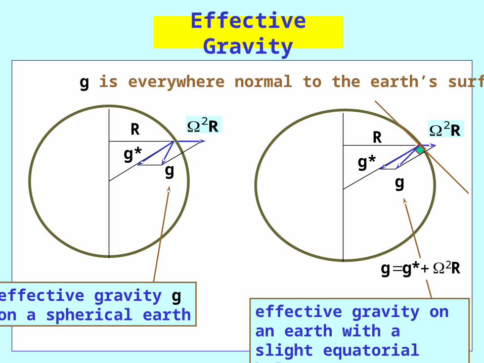
g is everywhere normal to the earth’s surface

Effective Gravity

2 g g* R

Effective Gravity

If the earth were a perfect sphere and not rotating, the only gravitational component g* would be radial.

Because the earth has a bulge and is rotating, the effective gravitational force g is the vector sum of the normal gravity to the mass distribution g*, together with a centrifugal force 2R, and this has no tangential component at the earth’s surface.

g g * R 2

When frictional forces can be neglected, F is the pressure gradient force

Tp F force per unit volume

d2

dt

uu F g

This is Euler’s equation of motion in a rotating reference frame.

total pressure

d

dtpT

u

12

g u per

unit mass

u

2 u

the Coriolis force acts normal to the rotation vector and normal to the velocity.

is directly proportional tothe magnitude of u and .

Note: the Coriolis force does no work because u ( u) 2 0

The Coriolis force does no work

Define p p z pT 0( ) where

p0(z) and 0(z) are reference pressure and density fields

p is the perturbation pressure

Euler’s equation becomes

dp

dzg0

0

D

Dtp

uu g

2

1 0

the buoyancy force

Perturbation pressure, buoyancy force

g = (0, 0, g)

But the total force is uniquely defined.

Important: the perturbation pressure gradient

and buoyancy forceare not uniquely defined.

01p

g

0

g

1

p

Indeed 0T

1 1p p

g g

u

v

v v

u u

w

w w

z

yx

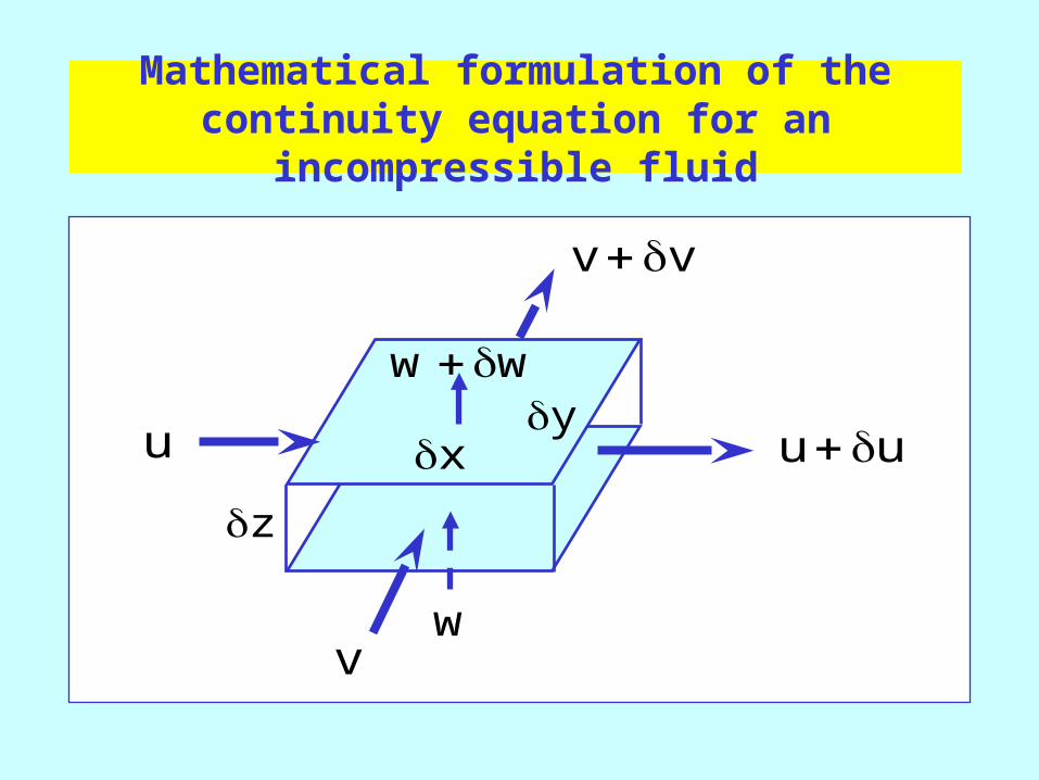
Mathematical formulation of the continuity equation for an incompressible fluid

The mass continuity equation

Compressible fluid

0 uIncompressible fluid

( ) 0t

u

( (z) ) 0o uAnelastic approximation

Rigid body dynamics

Force FMass m

x

2

2

d xm F

dtNewton’s equation of motion is:

Problem is to calculate x(t) given the force F

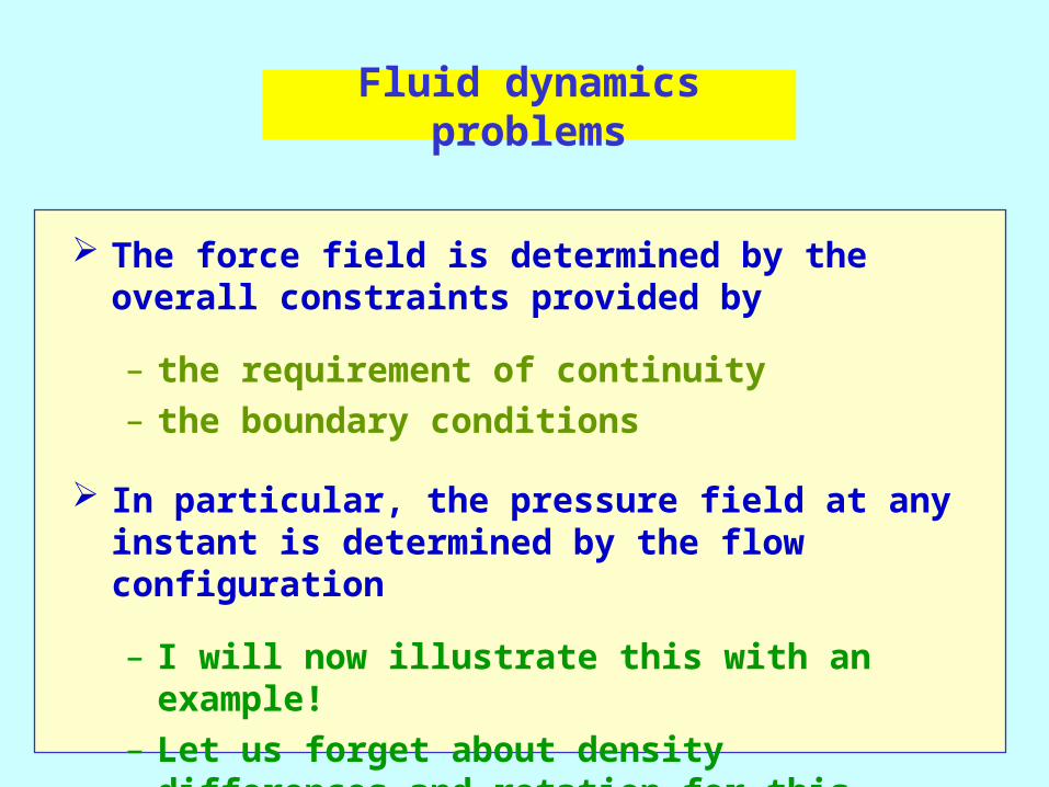
Fluid dynamics problems

The force field is determined by the overall constraints provided by

– the requirement of continuity

– the boundary conditions

In particular, the pressure field at any instant is determined by the flow configuration

– I will now illustrate this with an example!

– Let us forget about density differences and rotation for this example

Fluid dynamics problems

The aim of any fluid dynamics calculation is to calculate the flow field U(x,y,z,t) in a given region subject to appropriate boundary conditions and the constraint of continuity.

The calculation of the force field (i.e. the pressure field) may not be necessary, depending on the solution method.

U

U

pump

isobars

streamlines

HI

HI

LO

LO

HI

Assumptions: inviscid, irrotational, incompressible flow

A mathematical demonstration

D 1p '

Dt

u

Momentum equation Continuity equation

u 0

The divergence of the momentum equation gives:

2p ' u u

This is a diagnostic equation!

But what about the effects of rotation?

Newton’s 2nd law vertical component

TDw pg

Dt z

mass acceleration = force

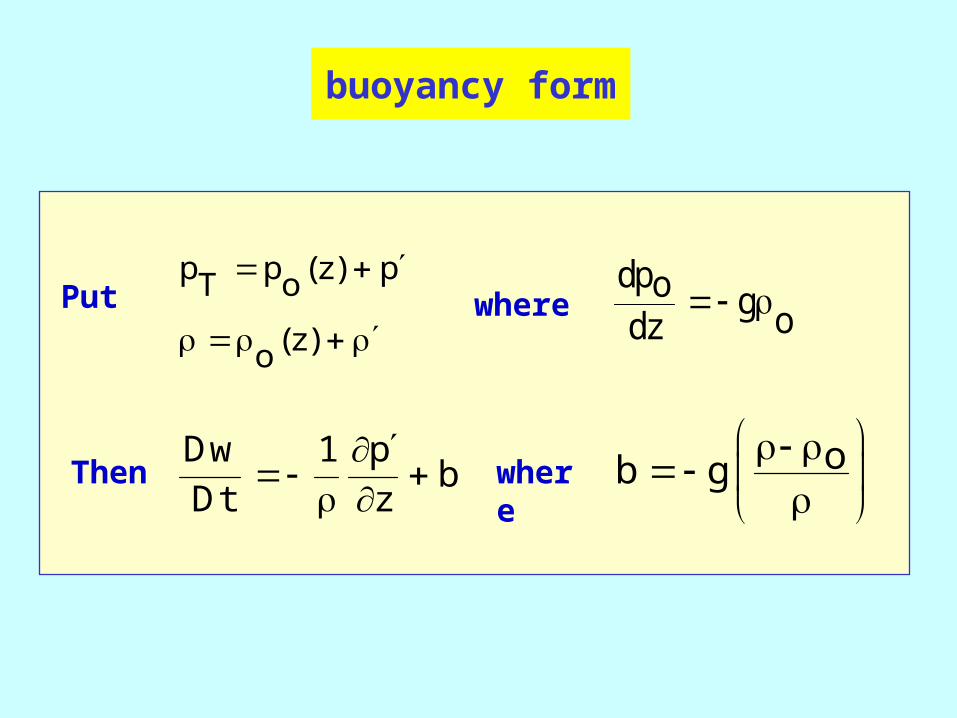
buoyancy form

Dw 1 pb

Dt z

p p (z) pT o

(z)o

Put

Then

wheredpo g odz

where ob g

buoyancy force is NOT unique

ob g

it depends on choice of reference density o(z)

but T1 p 1 p 'g b

z z

is unique

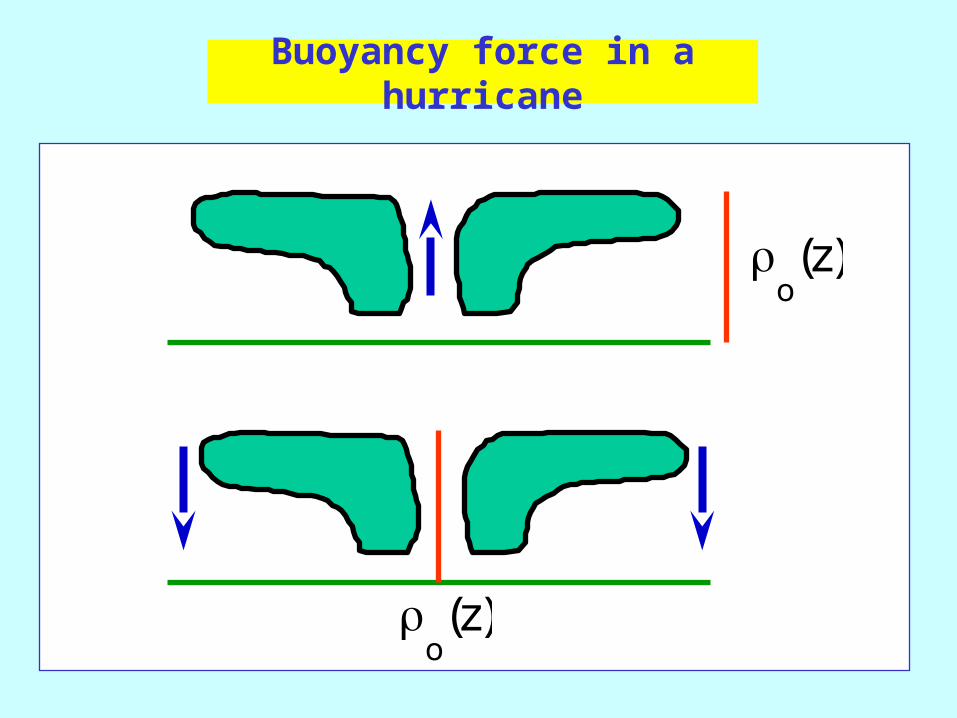
Buoyancy force in a hurricane

o

z( )

o

z( )

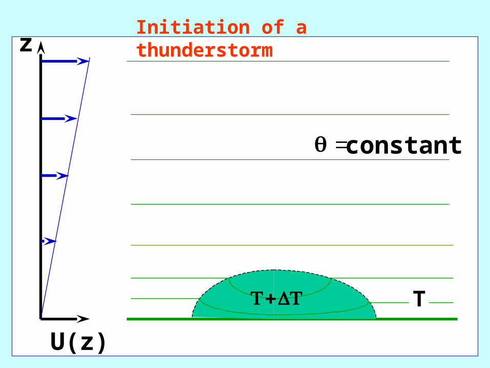
U(z)

z

constant

T

Initiation of a thunderstorm

= constant

tropopausenegative buoyancy

outflow

inflow

LCLLFC

original heated air

negative buoyancy

positivebuoyancy

Some questions

How does the flow evolve after the original thermal has reached the upper troposphere?

What drives the updraught at low levels?

– Observation in severe thunderstorms: the updraught at cloud base is negatively buoyant!

– Answer: - the perturbation pressure gradient

outflow

inflow

original heated air

negative buoyancy

LFC

LCL

positive buoyancy

HI

HI

HIHI

LO

p'

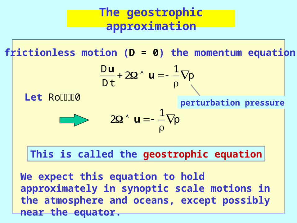
Let Ro0

21

u

p

For frictionless motion (D = 0) the momentum equation is

D

Dtp

u 2

1 u

This is called the geostrophic equation

We expect this equation to hold approximately in synoptic scale motions in the atmosphere and oceans, except possibly near the equator.

The geostrophic approximation

perturbation pressure

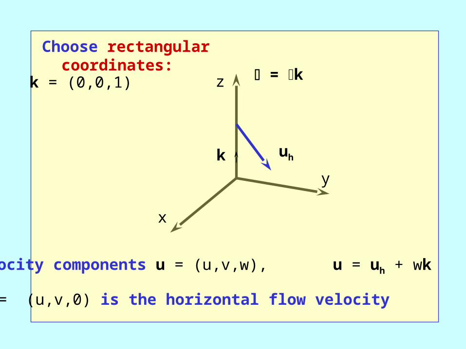
Choose rectangular coordinates:

z

uh

x

y

k

velocity components u = (u,v,w), u = uh + wk

= kk = (0,0,1)

uh = (u,v,0) is the horizontal flow velocity

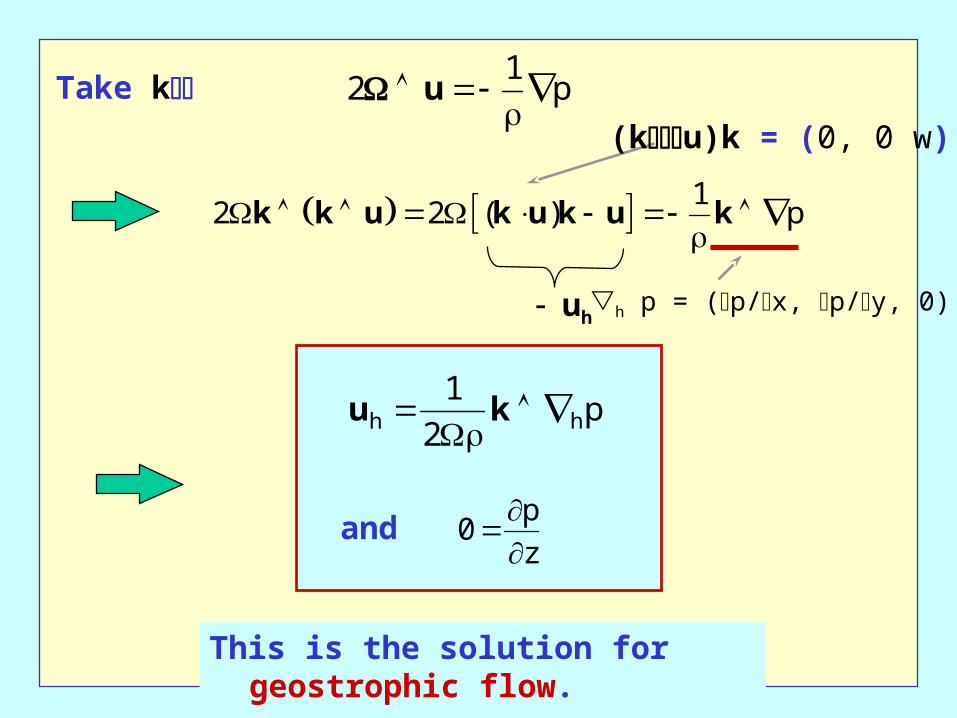
Take k

12 2 ( ) p

k k u k u k u k

21

u

p

(ku)k = (0, 0 w)

h p = (p/x, p/y, 0)

u kh hp 1

2

and 0 p

z

This is the solution for geostrophic flow.

uh

u kh hp 1

2

The geostrophic wind blows parallel to the lines (or more strictly surfaces) of constant pressure - the isobars, with low pressure to the left.

Well known to the layman who tries to interpret the newspaper "weather map", which is a chart showing isobaric lines at mean sea level.

In the southern hemisphere, low pressure is to the right.

The geostrophic wind

For simplicity, let us orientate the coordinates so that x points in the direction of the geostrophic wind.

Then v = 0, implying that p/x = 0 .

up

y

1

2

Note that for fixed , the winds are stronger when the isobars are closer together and, for a given isobar separation, they are stronger for smaller |.

Choice of coordinates

low p

high p

isobar

isobar

Coriolis force

pressure gradient force

u

(Northern hemisphere case: > 0)

Geostrophic flow

H H

L

H

A mean sea level isobaric chart over Australia

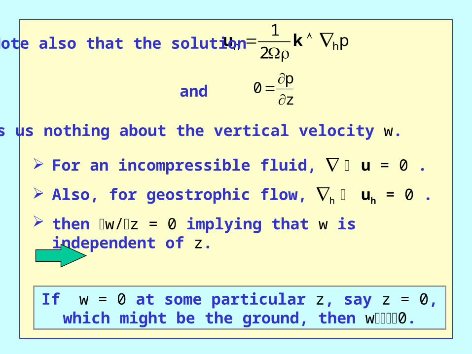
For an incompressible fluid, u = 0 .

Also, for geostrophic flow, h uh = 0 .

then w/z = 0 implying that w is independent of z.

u kh hp 1

2

and 0 p

z

Note also that the solution

tells us nothing about the vertical velocity w.

If w = 0 at some particular z, say z = 0, which might be the ground, then w0.

The geostrophic equation is degenerate, i.e. time derivatives have been eliminated in the approximation.

We cannot use the equation to predict how the flow will evolve.

Such equations are called diagnostic equations.

In the case of the geostrophic equation, for example, a knowledge of the isobar spacing at a given time allows us to calculate, or 'diagnose', the geostrophic wind.

We cannot use the equation to forecast how the wind velocity will change with time.

The geostrophic equation is degenerate!

Vortex flows: the gradient wind equation

Strict geostrophic motion requires that the isobars be straight, or, equivalently, that the flow be uni-directional.

To investigate balanced flows with curved isobars, including vortical flows, it is convenient to express Euler's equation in cylindrical coordinates.

To do this we need an expression for the total horizontal acceleration Duh/Dt in cylindrical coordinates.

The radial and tangential components of Euler's equation may be written

u

tu

u

r

v

r

uw

u

z

v

rfv

p

r

2 1

v

tu

v

r

v

r

vw

v

z

uv

rfu

r

p

1

The axial component is

w

tu

w

r

v

r

ww

w

z

p

z

1

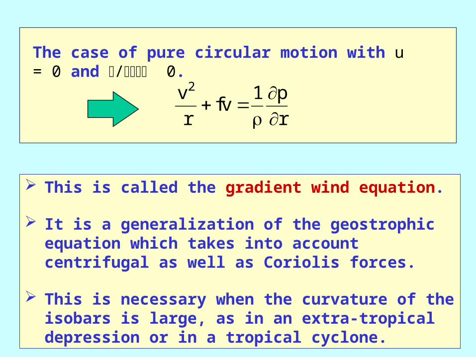
The case of pure circular motion with u = 0 and / 0.

v

rfv

p

r

2 1

This is called the gradient wind equation.

It is a generalization of the geostrophic equation which takes into account centrifugal as well as Coriolis forces.

This is necessary when the curvature of the isobars is large, as in an extra-tropical depression or in a tropical cyclone.

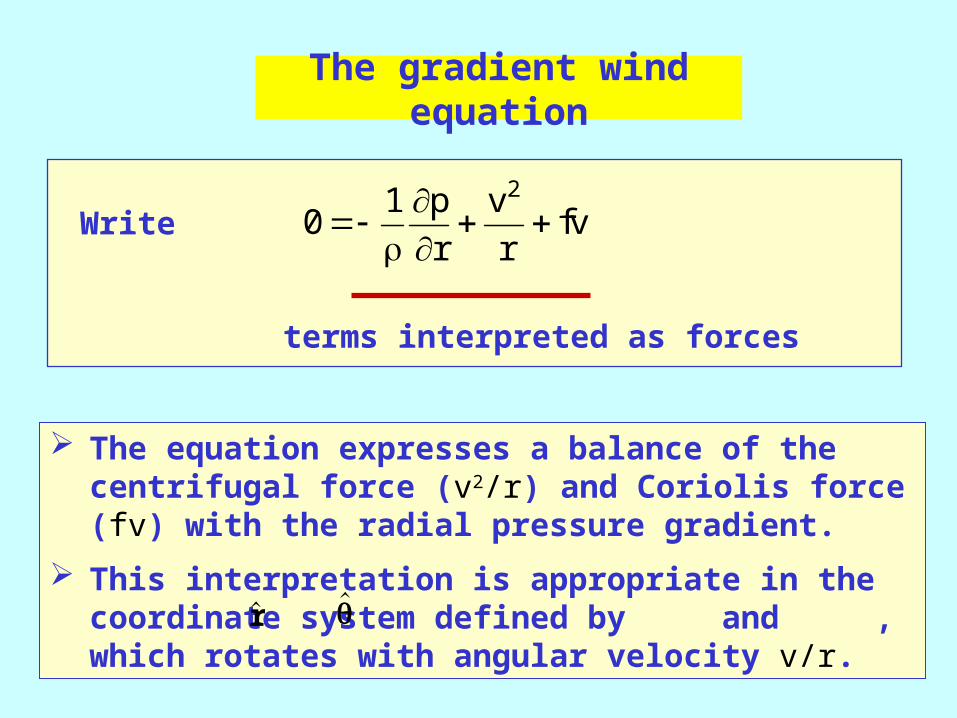
terms interpreted as forces

The equation expresses a balance of the centrifugal force (v2/r) and Coriolis force (fv) with the radial pressure gradient.

This interpretation is appropriate in the coordinate system defined by and , which rotates with angular velocity v/r.

01 2

p

r

v

rfv

Write

r

The gradient wind equation

V V

LO

LO

HI

HI

PG

PGCECE

COCO

Cyclone Anticyclone

Force balances in low and high pressure systems

is a diagnostic equation for the tangential velocity v in terms of the pressure gradient:

01 2

p

r

v

rfvThe equation

v fr f rr p

r

LNM

OQP

1

2

1

42 2

12

Choose the positive sign so that geostrophic balance is recovered as r(for finite v, the centrifugal force tends to zero as r ).

In a low pressure system, p/r > 0 and there is no theoretical limit to the tangential velocity v.

In a high pressure system, p/r < 0 and the local value of the pressure gradient cannot be less than rf2/4 in a balanced state.

Therefore the tangential wind speed cannot locally exceed rf/2 in magnitude.

This accords with observations in that wind speeds in anticyclones are generally light, whereas wind speeds in cyclones may be quite high.

v fr f rr p

r

LNM

OQP

1

2

1

42 2

12

In the anticyclone, the Coriolis force increases only in proportion to v: => this explains the upper limit on v predicted by the gradient wind equation.

V

HI

PG

CE

CO

CO fv

CEv

r

2

Limited wind speed in anticyclones

End of L2