Title stata.com

power logrank — Power analysis for the log-rank test

Description Quick start Menu SyntaxOptions Remarks and examples Stored results Methods and formulasReferences Also see

Description

power logrank computes sample size, power, or effect size for survival analysis comparingsurvivor functions in two groups by using the log-rank test. The results can be obtained using theFreedman or Schoenfeld approaches. Effect size can be expressed as a hazard ratio or as a log hazard-ratio. The command supports unbalanced designs, and provides options to account for administrativecensoring, uniform accrual, and withdrawal of subjects from the study.

Quick startSample size for a log-rank test of H0: ∆ = 0 versus Ha: ∆ 6= 0 using the Freedman method for

alternative hazard ratio ∆a = 0.76 without censoring and with default power of 0.8 and significancelevel α = 0.05

power logrank, hratio(.76)

As above, but use Schoenfeld’s methodpower logrank, hratio(.76) schoenfeld

Sample size for censored design with survival probabilities surv1 = 0.3 and surv2 = 0.4power logrank .3 .4

Same as above, specified as surv1 = 0.3 and hazard ratio of 0.76power logrank .3, hratio(.76)

As above, but for hazard ratios of 0.65, 0.7, 0.75, and 0.8power logrank .3, hratio(.65(.05).8)

As above, but show results in a graph of hazard ratio versus sample sizepower logrank .3, hratio(.65(.05).8) graph

Sample size for a one-sided test with α = 0.01power logrank .3, hratio(.76) onesided alpha(.01)

Sample size adjusted for 10% withdrawal from the studypower logrank .3, hratio(.76) wdprob(.1)

Power for a design with censoring and a sample size of 300power logrank .3 .4, n(300)

As above, but specify twice as many observations in the experimental grouppower logrank .3 .4, n(300) nratio(2)

1

2 power logrank — Power analysis for the log-rank test

Effect size for a design without censoring, sample size of 300, power of 0.8, and default α = 0.05power logrank, n(300) power(.8)

As above, but for a censored design with control-group survival probability of 0.3power logrank .3, n(300) power(.8)

MenuStatistics > Power and sample size

Syntax

Compute sample size

power logrank[

surv1

[surv2

] ] [, power(numlist) options

]

Compute power

power logrank[

surv1

[surv2

] ], n(numlist)

[options

]

Compute effect size

power logrank[

surv1

], n(numlist) power(numlist)

[options

]

where

surv1 is the survival probability in the control (reference) group at the end of the study t∗, and

surv2 is the survival probability in the experimental (comparison) group at the end of the study t∗.

surv1 and surv2 may each be specified either as one number or as a list of values in parentheses; see[U] 11.1.8 numlist.

power logrank — Power analysis for the log-rank test 3

options Description

Main∗alpha(numlist) significance level; default is alpha(0.05)∗power(numlist) power; default is power(0.8)∗beta(numlist) probability of type II error; default is beta(0.2)∗n(numlist) total sample size; required to compute power or effect size∗n1(numlist) sample size of the control group∗n2(numlist) sample size of the experimental group∗nratio(numlist) ratio of sample sizes, N2/N1; default is nratio(1), meaning

equal group sizesnfractional allow fractional sample sizes

∗hratio(numlist) hazard ratio (effect size) of the experimental to the controlgroup; default is hratio(0.5); may not be combined withlnhratio()

∗lnhratio(numlist) log hazard-ratio (effect size) of the experimental to the controlgroup; may not be combined with hratio()

schoenfeld use the formula based on the log hazard-ratioin calculations; default is to use the formula basedon the hazard ratio

effect(effect) specify the type of effect to display; default is method-specificdirection(lower|upper) direction of the effect for effect-size determination; default is

direction(lower), which means that the postulated valueof the parameter is smaller than the hypothesized value

onesided one-sided test; default is two sidedparallel treat number lists in starred options or in command arguments

as parallel when multiple values per option or argument arespecified (do not enumerate all possible combinations ofvalues)

Censoring

simpson(# # # |matname) survival probabilities in the control group at threespecific time points to compute the probability of an event(failure), using Simpson’s rule under uniform accrual

st1(varnames varnamet) variables varnames, containing survival probabilities inthe control group, and varnamet, containing respective timepoints, to compute the probability of an event (failure),using numerical integration under uniform accrual

∗wdprob(numlist) proportion of subjects anticipated to withdraw from thestudy; default is wdprob(0)

Table[no]table

[(tablespec)

]suppress table or display results as a table;

see [PSS] power, tablesaving(filename

[, replace

]) save the table data to filename; use replace to overwrite

existing filename

Graph

graph[(graphopts)

]graph results; see [PSS] power, graph

4 power logrank — Power analysis for the log-rank test

Iteration

init(#) initial value for effect sizeiterate(#) maximum number of iterations; default is iterate(500)

tolerance(#) parameter tolerance; default is tolerance(1e-12)

ftolerance(#) function tolerance; default is ftolerance(1e-12)[no]log suppress or display iteration log[

no]dots suppress or display iterations as dots

notitle suppress the title

∗Specifying a list of values in at least two starred options, or at least two command arguments, or at least onestarred option and one argument results in computations for all possible combinations of the values; see[U] 11.1.8 numlist. Also see the parallel option.

notitle does not appear in the dialog box.

effect Description

hratio hazard ratiolnhratio log hazard-ratio

where tablespec is

column[:label

] [column

[:label

] [. . .] ] [

, tableopts]

column is one of the columns defined below, and label is a column label (may contain quotes andcompound quotes).

column Description Symbol

alpha significance level αpower power 1− βbeta type II error probability βN total number of subjects NN1 number of subjects in the control group N1

N2 number of subjects in the experimental group N2

nratio ratio of sample sizes, experimental to control N2/N1

delta effect size δE total number of events (failures) Ehratio hazard ratio ∆lnhratio log hazard-ratio ln(∆)s1 survival probability in the control group S1(T )s2 survival probability in the experimental group S2(T )Pr E overall probability of an event (failure) pEPr w probability of withdrawals pwtarget target parameter; hratio or lnhratioall display all supported columns

power logrank — Power analysis for the log-rank test 5

Column beta is shown in the default table in place of column power if option beta() is specified.Column lnhratio is shown in the default table in place of column hratio if specified.Columns s1 and s2 are available only when specified.Columns nratio and Pr w are shown in the default table if specified.

Options

� � �Main �

alpha(), power(), beta(), n(), n1(), n2(), nratio(), nfractional; see [PSS] power.

hratio(numlist) specifies the hazard ratio (effect size) of the experimental group to the control group.The default is hratio(0.5). This value typically defines the clinically significant improvementof the experimental procedure over the control procedure desired to be detected by the log-ranktest with a certain power.

You can specify an effect size either as a hazard ratio in hratio() or as a log hazard-ratioin lnhratio(). The default is hratio(0.5). If both arguments surv1 and surv2 are specified,hratio() is not allowed and the hazard ratio is instead computed as ln(surv2)/ ln(surv1).

This option is not allowed with the effect-size determination and may not be combined withlnhratio().

lnhratio(numlist) specifies the log hazard-ratio (effect size) of the experimental group to the controlgroup. This value typically defines the clinically significant improvement of the experimentalprocedure over the control procedure desired to be detected by the log-rank test with a certainpower.

You can specify an effect size either as a hazard ratio in hratio() or as a log hazard-ratioin lnhratio(). The default is hratio(0.5). If both arguments surv1 and surv2 are specified,lnhratio() is not allowed and the log hazard-ratio is computed as ln{ ln(surv2)/ ln(surv1)}.This option is not allowed with the effect-size determination and may not be combined withhratio().

schoenfeld requests calculations using the formula based on the log hazard-ratio, according toSchoenfeld (1981). The default is to use the formula based on the hazard ratio, according toFreedman (1982).

effect(effect) specifies the type of the effect size to be reported in the output as delta. effect is oneof hratio or lnhratio. By default, the effect size delta is a hazard ratio, effect(hratio),for a hazard-ratio test and a log hazard-ratio, effect(lnhratio), for a log hazard-ratio test(when schoenfeld is specified).

direction(), onesided, parallel; see [PSS] power. direction(lower) is the default.

� � �Censoring �

simpson(# # # |matname) specifies survival probabilities in the control group at three specific timepoints to compute the probability of an event (failure) using Simpson’s rule under the assumptionof uniform accrual. Either the actual values or a 1× 3 matrix, matname, containing these valuescan be specified. By default, the probability of an event is approximated as an average of the failureprobabilities 1−s1 and 1−s2; see Methods and formulas. simpson() may not be combined withst1() and may not be used if command argument surv1 or surv2 is specified. This option is notallowed with effect-size computation.

6 power logrank — Power analysis for the log-rank test

st1(varnames varnamet) specifies variables varnames, containing survival probabilities in the controlgroup, and varnamet, containing respective time points, to compute the probability of an event(failure) using numerical integration under the assumption of uniform accrual; see [R] dydx. Theminimum and the maximum values of varnamet must be the length of the follow-up period andthe duration of the study, respectively. By default, the probability of an event is approximated asan average of the failure probabilities 1−s1 and 1−s2; see Methods and formulas. st1() maynot be combined with simpson() and may not be used if command argument surv1 or surv2 isspecified. This option is not allowed with effect-size computation.

wdprob(numlist) specifies the proportion of subjects anticipated to withdraw from the study. Thedefault is wdprob(0). wdprob() is allowed only with sample-size computation.

� � �Table �

table, table(), notable; see [PSS] power, table.

saving(); see [PSS] power.

� � �Graph �

graph, graph(); see [PSS] power, graph. Also see the column table for a list of symbols used bythe graphs.

� � �Iteration �

init(#) specifies an initial value for the estimated hazard ratio or, if schoenfeld is specified, forthe estimated log hazard-ratio during the effect-size determination.

iterate(), tolerance(), ftolerance(), log, nolog, dots, nodots; see [PSS] power.

The following option is available with power logrank but is not shown in the dialog box:

notitle; see [PSS] power.

Remarks and examples stata.com

Remarks are presented under the following headings:

IntroductionUsing power logrankComputing sample size

Computing sample size in the absence of censoringComputing sample size in the presence of censoringWithdrawal of subjects from the studyIncluding information about subject accrual

Computing powerComputing effect sizeTesting a hypothesis about two survivor functions using a log-rank test

This entry describes the power logrank command and the methodology for power and sample-sizeanalysis for a two-sample comparison of survivor functions using a log-rank test. See [PSS] intro fora general introduction to power and sample-size analysis and [PSS] power for a general introductionto the power command using hypothesis tests. See Survival data in [PSS] intro for an introductionto power and sample-size analysis for survival data.

power logrank — Power analysis for the log-rank test 7

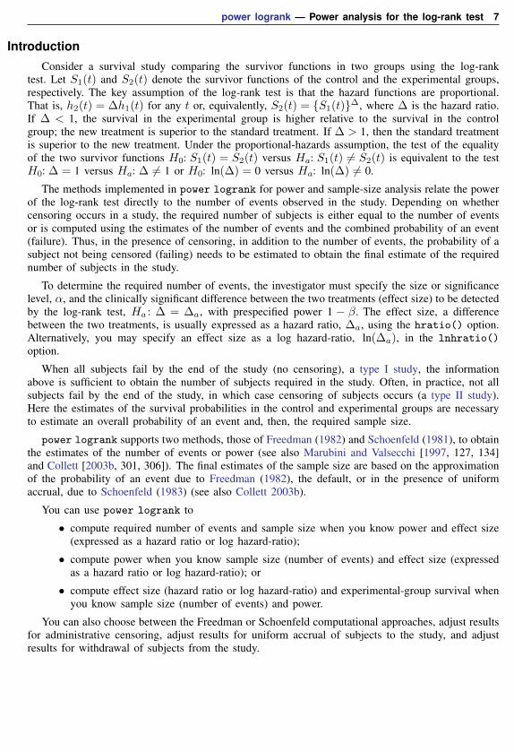
IntroductionConsider a survival study comparing the survivor functions in two groups using the log-rank

test. Let S1(t) and S2(t) denote the survivor functions of the control and the experimental groups,respectively. The key assumption of the log-rank test is that the hazard functions are proportional.That is, h2(t) = ∆h1(t) for any t or, equivalently, S2(t) = {S1(t)}∆, where ∆ is the hazard ratio.If ∆ < 1, the survival in the experimental group is higher relative to the survival in the controlgroup; the new treatment is superior to the standard treatment. If ∆ > 1, then the standard treatmentis superior to the new treatment. Under the proportional-hazards assumption, the test of the equalityof the two survivor functions H0: S1(t) = S2(t) versus Ha: S1(t) 6= S2(t) is equivalent to the testH0: ∆ = 1 versus Ha: ∆ 6= 1 or H0: ln(∆) = 0 versus Ha: ln(∆) 6= 0.

The methods implemented in power logrank for power and sample-size analysis relate the powerof the log-rank test directly to the number of events observed in the study. Depending on whethercensoring occurs in a study, the required number of subjects is either equal to the number of eventsor is computed using the estimates of the number of events and the combined probability of an event(failure). Thus, in the presence of censoring, in addition to the number of events, the probability of asubject not being censored (failing) needs to be estimated to obtain the final estimate of the requirednumber of subjects in the study.

To determine the required number of events, the investigator must specify the size or significancelevel, α, and the clinically significant difference between the two treatments (effect size) to be detectedby the log-rank test, Ha : ∆ = ∆a, with prespecified power 1 − β. The effect size, a differencebetween the two treatments, is usually expressed as a hazard ratio, ∆a, using the hratio() option.Alternatively, you may specify an effect size as a log hazard-ratio, ln(∆a), in the lnhratio()option.

When all subjects fail by the end of the study (no censoring), a type I study, the informationabove is sufficient to obtain the number of subjects required in the study. Often, in practice, not allsubjects fail by the end of the study, in which case censoring of subjects occurs (a type II study).Here the estimates of the survival probabilities in the control and experimental groups are necessaryto estimate an overall probability of an event and, then, the required sample size.

power logrank supports two methods, those of Freedman (1982) and Schoenfeld (1981), to obtainthe estimates of the number of events or power (see also Marubini and Valsecchi [1997, 127, 134]and Collett [2003b, 301, 306]). The final estimates of the sample size are based on the approximationof the probability of an event due to Freedman (1982), the default, or in the presence of uniformaccrual, due to Schoenfeld (1983) (see also Collett 2003b).

You can use power logrank to

• compute required number of events and sample size when you know power and effect size(expressed as a hazard ratio or log hazard-ratio);

• compute power when you know sample size (number of events) and effect size (expressedas a hazard ratio or log hazard-ratio); or

• compute effect size (hazard ratio or log hazard-ratio) and experimental-group survival whenyou know sample size (number of events) and power.

You can also choose between the Freedman or Schoenfeld computational approaches, adjust resultsfor administrative censoring, adjust results for uniform accrual of subjects to the study, and adjustresults for withdrawal of subjects from the study.

8 power logrank — Power analysis for the log-rank test

Using power logrank

power logrank computes sample size, power, or effect size for the log-rank test comparing thesurvivor functions in two groups. All computations are performed for a two-sided hypothesis testwhere, by default, the significance level is set to 0.05. You may change the significance level byspecifying the alpha() option. You can specify the onesided option to request a one-sided test.By default, all computations assume a balanced- or equal-allocation design; see [PSS] unbalanceddesigns for a description of how to specify an unbalanced design.

To compute a total sample size, you specify an effect size and optionally power of the test in thepower() option. The default power is set to 0.8. By default, the computed sample size is roundedup. You can specify the nfractional option to see the corresponding fractional sample size; seeFractional sample sizes in [PSS] unbalanced designs for an example. The nfractional option isallowed only for sample-size determination.

To compute power, you must specify the total sample size in the n() option and an effect size.

An effect size may be specified either as a hazard ratio supplied in the hratio() option or as alog hazard-ratio supplied in the lnhratio() option. If neither is specified, a hazard ratio of 0.5 isassumed.

To compute an effect size, which may be expressed either as a hazard ratio or as a log hazard-ratio,you must specify the total sample size in the n() option; the power in the power() option; and,optionally, the direction of the effect. The direction is lower by default, direction(lower), whichmeans that the target hazard ratio is assumed to be less than one or that target log hazard-ratio isnegative. In other words, the experimental treatment is presumed to be an improvement over thecontrol treatment. If you want to change the direction to upper, corresponding to the target hazardratio being greater than one, use direction(upper).

Instead of the total sample size n(), you can specify individual group sizes in n1() and n2(), orspecify one of the group sizes and nratio() when computing power or effect size. Also see Twosamples in [PSS] unbalanced designs for more details.

As we mentioned earlier, the effect size for power logrank may be expressed as a hazard ratio oras a log hazard-ratio. By default, the effect size, which is labeled as delta in the output, correspondsto the hazard ratio for the Freedman method and to the log hazard-ratio for the Schoenfeld method.You can change this by specifying the effect() option: effect(hratio) (the default) reports thehazard ratio and effect(lnhratio) reports the log hazard-ratio.

By default, all computations assume no censoring. In the presence of administrative censoring, youmust specify a survival probability at the end of the study in the control group as the first commandargument. You can also specify a survival probability at the end of the study in the experimentalgroup as the second command argument. Otherwise, it will be computed using the specified hazardratio or log hazard-ratio and the control-group survival probability. To accommodate an accrual periodunder the assumption of uniform accrual, survival information may instead be supplied in optionsimpson() or in option st1(); see Including information about subject accrual for details.

When computing sample size, you can adjust for withdrawal of subjects from the study by specifyingthe anticipated proportion of withdrawals in the wdprob() option.

By default, power logrank performs computations for a hazard-ratio test. Use the schoenfeldoption to request computations for a log-hazard-ratio test.

In the presence of censoring, effect-size determination requires iteration. The default initial valueof the estimated hazard ratio or, if schoenfeld is specified, of log hazard-ratio is obtained based onthe formula assuming no censoring. This value may be changed by specifying the init() option.See [PSS] power for the descriptions of other options that control the iteration procedure.

power logrank — Power analysis for the log-rank test 9

In the following sections, we describe the use of power logrank accompanied by examples forcomputing sample size, power, and effect size.

Computing sample size

To compute sample size and number of events, you must specify an effect size (a hazard ratio ora log hazard-ratio) and, optionally, the power of the test in the power() option. A default power of0.8 is assumed if power() is not specified. A hazard ratio of 0.5 is assumed if an effect size is notspecified.

Computing sample size in the absence of censoring

We demonstrate several examples of how to use power logrank to obtain the estimates of samplesize and number of events using Freedman (1982) and Schoenfeld (1981) methods for uncensoreddata (a type I study when no censoring of subjects occurs).

Example 1: Number of events (failures) using Freedman method

Consider a survival study to be conducted to compare the survivor function of subjects receiving atreatment (the experimental group) to the survivor function of those receiving a placebo or no treatment(the control group) using the log-rank test. Suppose that the study continues until all subjects fail(no censoring). The investigator wants to know how many events need to be observed in the studyto achieve a power of 80% of a two-sided log-rank test with α = 0.05 to detect a 50% reduction inthe hazard of the experimental group (∆a = 0.5). Because the default settings of power logrankare power(0.8), alpha(0.05), and hratio(0.5), to obtain the estimate of the required numberof events for the above study using the Freedman method (the default), we simply type

. power logrank

Estimated sample sizes for two-sample comparison of survivor functionsLog-rank test, Freedman methodHo: HR = 1 versus Ha: HR != 1

Study parameters:

alpha = 0.0500power = 0.8000delta = 0.5000 (hazard ratio)

hratio = 0.5000

Censoring:

Pr_E = 1.0000

Estimated number of events and sample sizes:

E = 72N = 72

N per group = 36

From the output, a total of 72 events (failures) must be observed to achieve the required power of80%. Because all subjects experience an event by the end of the study (Pr E=1.0000), the number ofsubjects required to be recruited to the study is equal to the number of events. That is, the investigatorneeds to recruit a total of 72 subjects (36 per group) to the study.

10 power logrank — Power analysis for the log-rank test

Example 2: Number of events (failures) using Schoenfeld method

Following example 1, we can request the Schoenfeld method by specifying the schoenfeld option.

. power logrank, schoenfeld

Estimated sample sizes for two-sample comparison of survivor functionsLog-rank test, Schoenfeld methodHo: ln(HR) = 0 versus Ha: ln(HR) != 0

Study parameters:

alpha = 0.0500power = 0.8000delta = -0.6931 (log hazard-ratio)

hratio = 0.5000

Censoring:

Pr_E = 1.0000

Estimated number of events and sample sizes:

E = 66N = 66

N per group = 33

We obtain a slightly smaller estimate (66) of the total number of events and subjects.

Technical noteFreedman (1982) and Schoenfeld (1981) derive the formulas for the number of events based on

the asymptotic distribution of the log-rank test statistic. Freedman (1982) uses the asymptotic meanand variance of the log-rank test statistic expressed as a function of the true hazard ratio, ∆, whereasSchoenfeld (1981) (see also Collett [2003b, 302]) bases the derivation on the asymptotic mean of thelog-rank test statistic as a function of the true log hazard-ratio, ln(∆). We label the correspondingapproaches as “Freedman method” and “Schoenfeld method” in the output.

For values of the hazard ratio close to one, the two methods tend to give similar results. In general,the Freedman method gives higher estimates than the Schoenfeld method. The performance of theFreedman method was studied by Lakatos and Lan (1992) and was found to slightly overestimate thesample size under the assumption of proportional hazards. Hsieh (1992) investigated the performanceof the two methods under unequal allocation and concluded that Freedman’s formula predicts thehighest power for the log-rank test when the sample-size ratio of the two groups equals the reciprocalof the hazard ratio. Schoenfeld’s formula predicts highest powers when sample sizes in the two groupsare equal.

power logrank — Power analysis for the log-rank test 11

Example 3: Unbalanced design

By default, power logrank computes sample size for a balanced- or equal-allocation design. Ifwe know the allocation ratio of subjects between the groups, we can compute the required samplesize and number of events for an unbalanced design by specifying the nratio() option.

Continuing with example 1, we anticipate being able to recruit twice as many subjects in theexperimental group; that is, n2/n1 = 2. We specify the nratio(2) option to compute the requiredsample size for the specified unbalanced design.

. power logrank, nratio(2)

Estimated sample sizes for two-sample comparison of survivor functionsLog-rank test, Freedman methodHo: HR = 1 versus Ha: HR != 1

Study parameters:

alpha = 0.0500power = 0.8000delta = 0.5000 (hazard ratio)

hratio = 0.5000N2/N1 = 2.0000

Censoring:

Pr_E = 1.0000

Estimated number of events and sample sizes:

E = 63N = 63

N1 = 21N2 = 42

We need a total of 63 subjects—21 in the control group and 42 in the experimental group.

Also see Two samples in [PSS] unbalanced designs for more examples of unbalanced designs fortwo-sample tests.

Computing sample size in the presence of censoring

Because of constraints on costs and time, it is often infeasible to continue the study until allsubjects experience an event. Instead, the study terminates at some prespecified point in time. As aresult, some subjects may not experience an event by the end of the study; that is, administrativecensoring of subjects occurs. This increases the requirement on the number of subjects in the studyto ensure that a certain number of events is observed.

In the presence of censoring (for a type II study), Freedman (1982) assumes the following. Theanalysis occurs at a fixed time t∗ after the last patient was accrued, and all information about subjectfollow-up beyond time t∗ is excluded. To minimize an overestimation of the sample size becauseof neglecting this information, the author suggests choosing t∗ as the minimum follow-up time, f ,beyond which the frequency of occurrence of events is low (the time at which, say, 85% of thetotal events expected are observed). Under this assumption, the number of required subjects does notdepend on the rates of accrual and occurrence of events but only on the proportions of patients in thetwo treatment groups, s1 and s2, surviving after f . See Including information about subject accrualabout how to compute the sample size in the presence of a long accrual.

If censoring of subjects occurs, the probability of a subject not being censored needs to be estimatedto obtain an accurate estimate of the required sample size. The assumption above justifies a simpleprocedure, suggested by Freedman (1982) and used by default by power logrank, to compute

12 power logrank — Power analysis for the log-rank test

this probability using the estimates of survival probabilities at the end of the study in the controland the experimental groups. Therefore, for a type II study (under administrative censoring), theseprobabilities must be supplied to power logrank.

Example 4: Sample size in the presence of censoring using Freedman method

Consider an example from Machin et al. (2009, 91) of a study of patients with resectable coloncancer. The goal of the study was to compare the efficacy of the drug levamisole against a placebowith respect to relapse-free survival, using a one-sided log-rank test with a significance level of 5%.The investigators anticipated a 10% increase (from 50% to 60%, with a respective hazard ratio of0.737) in the survival of the experimental group with respect to the survival of the control (placebo)group at the end of the study. They wanted to detect this increase with a power of 80%. To obtainthe required sample size, we enter the survival probabilities 0.5 and 0.6 as arguments and specify theonesided option to request a one-sided test.

. power logrank 0.5 0.6, onesided

Estimated sample sizes for two-sample comparison of survivor functionsLog-rank test, Freedman methodHo: HR = 1 versus Ha: HR < 1

Study parameters:

alpha = 0.0500power = 0.8000delta = 0.7370 (hazard ratio)

hratio = 0.7370

Censoring:

s1 = 0.5000s2 = 0.6000

Pr_E = 0.4500

Estimated number of events and sample sizes:

E = 270N = 600

N per group = 300

From the above output, the investigators would have to observe a total of 270 events (relapses) todetect a 26% decrease in the hazard (∆a = 0.737) of the experimental group relative to the hazard ofthe control group with a power of 80% using a one-sided log-rank test with α = 0.05. They wouldhave to recruit a total of 600 patients (300 per group) to observe that many events.

In contrast, in the absence of censoring, only 270 subjects would have been required to detect adecrease in hazard corresponding to ∆a = 0.737:

power logrank — Power analysis for the log-rank test 13

. power logrank, hratio(0.737) onesided

Estimated sample sizes for two-sample comparison of survivor functionsLog-rank test, Freedman methodHo: HR = 1 versus Ha: HR < 1

Study parameters:

alpha = 0.0500power = 0.8000delta = 0.7370 (hazard ratio)

hratio = 0.7370

Censoring:

Pr_E = 1.0000

Estimated number of events and sample sizes:

E = 270N = 270

N per group = 135

Example 5: Sample size in the presence of censoring using Schoenfeld method

If we wanted to use the Schoenfeld method to calculate sample size for the study described inexample 4, we could type

. power logrank 0.5 0.6, onesided schoenfeld

Estimated sample sizes for two-sample comparison of survivor functionsLog-rank test, Schoenfeld methodHo: ln(HR) = 0 versus Ha: ln(HR) < 0

Study parameters:

alpha = 0.0500power = 0.8000delta = -0.3052 (log hazard-ratio)

hratio = 0.7370

Censoring:

s1 = 0.5000s2 = 0.6000

Pr_E = 0.4500

Estimated number of events and sample sizes:

E = 266N = 590

N per group = 295

We find that 590 subjects are required in the study to observe a total of 266 events to ensure a powerof 80%.

See the technical note in Computing sample size in the absence of censoring for a brief comparisonof the Freedman and Schoenfeld methods.

14 power logrank — Power analysis for the log-rank test

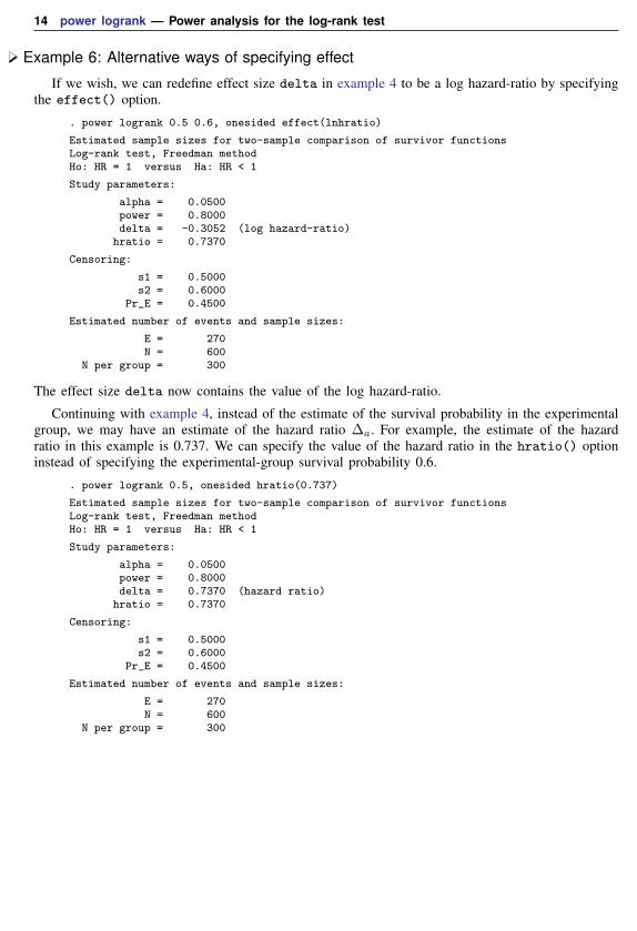
Example 6: Alternative ways of specifying effect

If we wish, we can redefine effect size delta in example 4 to be a log hazard-ratio by specifyingthe effect() option.

. power logrank 0.5 0.6, onesided effect(lnhratio)

Estimated sample sizes for two-sample comparison of survivor functionsLog-rank test, Freedman methodHo: HR = 1 versus Ha: HR < 1

Study parameters:

alpha = 0.0500power = 0.8000delta = -0.3052 (log hazard-ratio)

hratio = 0.7370

Censoring:

s1 = 0.5000s2 = 0.6000

Pr_E = 0.4500

Estimated number of events and sample sizes:

E = 270N = 600

N per group = 300

The effect size delta now contains the value of the log hazard-ratio.

Continuing with example 4, instead of the estimate of the survival probability in the experimentalgroup, we may have an estimate of the hazard ratio ∆a. For example, the estimate of the hazardratio in this example is 0.737. We can specify the value of the hazard ratio in the hratio() optioninstead of specifying the experimental-group survival probability 0.6.

. power logrank 0.5, onesided hratio(0.737)

Estimated sample sizes for two-sample comparison of survivor functionsLog-rank test, Freedman methodHo: HR = 1 versus Ha: HR < 1

Study parameters:

alpha = 0.0500power = 0.8000delta = 0.7370 (hazard ratio)

hratio = 0.7370

Censoring:

s1 = 0.5000s2 = 0.6000

Pr_E = 0.4500

Estimated number of events and sample sizes:

E = 270N = 600

N per group = 300

power logrank — Power analysis for the log-rank test 15

Alternatively, instead of the hazard ratio we can specify the log hazard-ratio in option lnhratio().

. power logrank 0.5, onesided lnhratio(-0.3052)

Estimated sample sizes for two-sample comparison of survivor functionsLog-rank test, Freedman methodHo: HR = 1 versus Ha: HR < 1

Study parameters:

alpha = 0.0500power = 0.8000delta = 0.7370 (hazard ratio)

ln(hratio) = -0.3052

Censoring:

s1 = 0.5000s2 = 0.6000

Pr_E = 0.4500

Estimated number of events and sample sizes:

E = 270N = 600

N per group = 300

The results are identical to the prior results. The estimate of the log hazard-ratio is now displayed inthe output instead of the hazard ratio.

Withdrawal of subjects from the study

Under administrative censoring, the subject is known to have experienced either of the two outcomesby the end of the study: survival or failure. Often, in practice, subjects may withdraw from the studybefore it terminates and therefore may not experience an event by the end of the study (or be censored)for nonadministrative reasons. Withdrawal of subjects from a study may greatly affect the estimate ofthe sample size and must be accounted for in the computations. Refer to Survival data in [PSS] introand [PSS] Glossary for a formal definition of withdrawal.

Freedman (1982) suggests a conservative adjustment for the estimate of the sample size in thepresence of withdrawal, which is implemented in power logrank. Withdrawal is assumed to beindependent of failure (event) times and administrative censoring.

The proportion of subjects anticipated to withdraw from a study may be specified by usingwdprob().

16 power logrank — Power analysis for the log-rank test

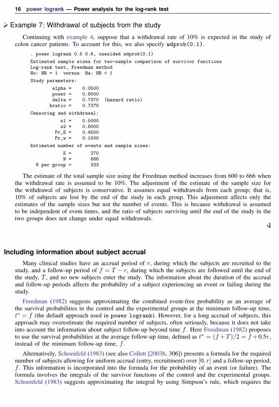
Example 7: Withdrawal of subjects from the study

Continuing with example 4, suppose that a withdrawal rate of 10% is expected in the study ofcolon cancer patients. To account for this, we also specify wdprob(0.1).

. power logrank 0.5 0.6, onesided wdprob(0.1)

Estimated sample sizes for two-sample comparison of survivor functionsLog-rank test, Freedman methodHo: HR = 1 versus Ha: HR < 1

Study parameters:

alpha = 0.0500power = 0.8000delta = 0.7370 (hazard ratio)

hratio = 0.7370

Censoring and withdrawal:

s1 = 0.5000s2 = 0.6000

Pr_E = 0.4500Pr_w = 0.1000

Estimated number of events and sample sizes:

E = 270N = 666

N per group = 333

The estimate of the total sample size using the Freedman method increases from 600 to 666 whenthe withdrawal rate is assumed to be 10%. The adjustment of the estimate of the sample size forthe withdrawal of subjects is conservative. It assumes equal withdrawals from each group; that is,10% of subjects are lost by the end of the study in each group. This adjustment affects only theestimates of the sample sizes but not the number of events. This is because withdrawal is assumedto be independent of event times, and the ratio of subjects surviving until the end of the study in thetwo groups does not change under equal withdrawals.

Including information about subject accrual

Many clinical studies have an accrual period of r, during which the subjects are recruited to thestudy, and a follow-up period of f = T − r, during which the subjects are followed until the end ofthe study, T , and no new subjects enter the study. The information about the duration of the accrualand follow-up periods affects the probability of a subject experiencing an event or failing during thestudy.

Freedman (1982) suggests approximating the combined event-free probability as an average ofthe survival probabilities in the control and the experimental groups at the minimum follow-up time,t∗ = f (the default approach used in power logrank). However, for a long accrual of subjects, thisapproach may overestimate the required number of subjects, often seriously, because it does not takeinto account the information about subject follow-up beyond time f . Here Freedman (1982) proposesto use the survival probabilities at the average follow-up time, defined as t∗ = (f +T )/2 = f + 0.5r,instead of the minimum follow-up time, f .

Alternatively, Schoenfeld (1983) (see also Collett [2003b, 306]) presents a formula for the requirednumber of subjects allowing for uniform accrual (entry, recruitment) over [0, r] and a follow-up period,f . This information is incorporated into the formula for the probability of an event (or failure). Theformula involves the integrals of the survivor functions of the control and the experimental groups.Schoenfeld (1983) suggests approximating the integral by using Simpson’s rule, which requires the

power logrank — Power analysis for the log-rank test 17

estimates of the survivor function at three specific time points: f , 0.5r + f , and T = r + f . It issufficient to provide the estimates of these three survival probabilities, S1(f), S1(0.5r + f), andS1(T ), for the control group only. The corresponding survival probabilities of the experimental groupare automatically computed using the value of the hazard ratio in hratio() (or log hazard-ratio inlnhratio()) and the proportional-hazards assumption.

The three estimates of the survival probabilities of the control group may be supplied by usingthe simpson() option to adjust the estimates of the sample size or power for uniform entry anda follow-up period. If the estimate of the survivor function over an array of values in the range[f, T ] is available from a previous study, it can be supplied using the st1() option to form a moreaccurate approximation of the probability of an event using numerical integration (see [R] dydx).Here the value of the length of the accrual period is needed for the computation. It is computed as thedifference between the maximum and the minimum values of the time variable varnamet, suppliedusing st1(), that is, r = T − f = max(varnamet)− min(varnamet).

For more information, see Cleves, Gould, and Marchenko (2016, sec. 16.2).

Example 8: Sample size in the presence of accrual and follow-up periods

Consider an example described in Collett (2003b, 309) of a survival study of chronic activehepatitis. A new treatment is to be compared with a standard treatment with respect to the survivaltimes of the patients with this disease. The investigators want to detect a change in a hazard ratio of0.57 with 90% power and a 5% two-sided significance level. Also subjects are to be entered into thestudy uniformly over a period of 18 months and then followed for 24 months. From the Kaplan–Meierestimate of the survivor function available for the control group, the survival probabilities at f = 24,0.5r + f = 33, and T = 42 months are 0.70, 0.57, and 0.45, respectively.

. power logrank, hratio(0.57) power(0.9) schoenfeld simpson(0.7 0.57 0.45)note: probability of an event is computed using Simpson’s rule with

S1(f) = 0.70, S1(f+r/2) = 0.57, S1(T) = 0.45S2(f) = 0.82, S2(f+r/2) = 0.73, S2(T) = 0.63

Estimated sample sizes for two-sample comparison of survivor functionsLog-rank test, Schoenfeld methodHo: ln(HR) = 0 versus Ha: ln(HR) != 0

Study parameters:

alpha = 0.0500power = 0.9000delta = -0.5621 (log hazard-ratio)

hratio = 0.5700

Censoring:

Pr_E = 0.3514

Estimated number of events and sample sizes:

E = 134N = 380

N per group = 190

Collett (2003b, 305) reports the required number of events to be 133, which, apart from rounding,agrees with our estimate of 134. In a later example, Collett (2003, 309) uses the number of events,rounded to 140, to compute the required sample size as 140/0.35 = 400, where 0.35 is the estimate ofthe combined probability of an event. By hand, without rounding the number of events, we computethe required sample size as 133/0.35 = 380 and obtain the same estimate of the total sample size asin the output.

18 power logrank — Power analysis for the log-rank test

Using the average follow-up time suggested by Freedman (1982), we obtain the following:. power logrank 0.57, hratio(0.57) power(0.9) schoenfeld

Estimated sample sizes for two-sample comparison of survivor functionsLog-rank test, Schoenfeld methodHo: ln(HR) = 0 versus Ha: ln(HR) != 0

Study parameters:

alpha = 0.0500power = 0.9000delta = -0.5621 (log hazard-ratio)

hratio = 0.5700

Censoring:

s1 = 0.5700s2 = 0.7259

Pr_E = 0.3521

Estimated number of events and sample sizes:

E = 134N = 378

N per group = 189

We specify the survival probability in the control group at t∗ = 0.5r + f = 0.5× 18 + 24 = 33as S1(33) = 0.57 and the hazard ratio of 0.57 (coincidentally). The survival probability in theexperimental group is S2(33) = S1(33)∆ = 0.570.57 = 0.726. Here we obtain the estimate ofthe sample size, 378, which is close to the estimate of 380 computed using the more complicatedapproximation. In this example, the two approximations produce similar results, but this may notalways be the case.

The approximation suggested by Schoenfeld (1983) and Collett (2003b) is considered to be moreaccurate because it takes into account information about the patient survival beyond the averagefollow-up time. In general, the Freedman (1982) and Schoenfeld (1983) approximations tend to givesimilar results when {S̃(f) + S̃(T )}/2 ≈ S̃(0.5r + f); see Methods and formulas for a formaldefinition of S̃(·).

If we use the survival probability in the control group, S1(24) = 0.7, at a follow-up timet∗ = f = 24 instead of the average follow-up time t∗ = 33 in the presence of an accrual period,

. power logrank 0.7, hratio(0.57) power(0.9) schoenfeld

Estimated sample sizes for two-sample comparison of survivor functionsLog-rank test, Schoenfeld methodHo: ln(HR) = 0 versus Ha: ln(HR) != 0

Study parameters:

alpha = 0.0500power = 0.9000delta = -0.5621 (log hazard-ratio)

hratio = 0.5700

Censoring:

s1 = 0.7000s2 = 0.8160

Pr_E = 0.2420

Estimated number of events and sample sizes:

E = 134N = 550

N per group = 275

we obtain the estimate of the total sample size of 550, which is substantially greater than the previouslyestimated sample sizes of 380 and 378.

power logrank — Power analysis for the log-rank test 19

Computing power

Sometimes the number of subjects available for the enrollment into the study is limited. In suchcases, the researchers may want to investigate with what power they can detect a desired treatmenteffect for a given sample size.

To compute power, you must specify the sample size in the n() option and an effect size (a hazardratio or a log hazard-ratio). A hazard ratio of 0.5 is assumed if an effect size is not specified.

Example 9: Power determination

Recall the colon cancer study described in example 4. Suppose that only 100 subjects are availableto be recruited to the study. We find out how this affects the power to detect a hazard ratio of 0.737.

. power logrank 0.5, hratio(0.737) onesided n(100)

Estimated power for two-sample comparison of survivor functionsLog-rank test, Freedman methodHo: HR = 1 versus Ha: HR < 1

Study parameters:

alpha = 0.0500N = 100

N per group = 50delta = 0.7370 (hazard ratio)

hratio = 0.7370

Number of events and censoring:

E = 46s1 = 0.5000s2 = 0.6000

Pr_E = 0.4500

Estimated power:

power = 0.2646

The power to detect an alternative Ha: ∆ = 0.737 decreased from 0.8 to 0.2646 when the samplesize decreased from 600 to 100 (the number of events decreased from 270 to 46).

Example 10: Multiple values of study parameters

Continuing with example 9, suppose we want to consider a range of sample sizes. We can specifya list (see [U] 11.1.8 numlist) of sample sizes in the n() option. For simplicity, we display onlypower, sample size, and number of events in the table.

. power logrank 0.5, hratio(0.737) onesided n(100(100)600) table(power N E)

Estimated power for two-sample comparison of survivor functionsLog-rank test, Freedman methodHo: HR = 1 versus Ha: HR < 1

power N E

.2646 100 46

.4174 200 91

.5455 300 136

.6505 400 181

.7344 500 226

.8004 600 271

20 power logrank — Power analysis for the log-rank test

As the sample size increases, the power increases. The decrease in sample size reduces the numberof events observed in the study and therefore changes the estimates of the power. If the number ofevents were fixed, power would have been independent of the sample size, provided that all otherparameters were held constant, because the formulas relate power directly to the number of eventsand not the number of subjects.

For multiple values of parameters, the results are automatically displayed in a table, as we seeabove. For more examples of tables, see [PSS] power, table. If you wish to produce a power plot,see [PSS] power, graph.

Computing effect size

Effect size δ for a log-rank test comparing two survivor functions is defined as a hazard ratio (ora log hazard-ratio) of the experimental group to the control group. This value typically defines theclinically significant improvement of the experimental procedure over the control procedure desiredto be detected by the log-rank test with a certain power.

Sometimes, we may be interested in determining the smallest effect that yields a statisticallysignificant result for prespecified sample size and power. In this case, both power and sample sizemust be specified in options power() and n(), respectively. Additionally, you may also choose thedirection of the effect by specifying the direction() option. direction(lower) is the default,and it assumes ∆a < 1 [or ln(∆a) < 0]. You can use direction(upper) to compute ∆a > 1 [orln(∆a) > 0].

Example 11: Effect-size determination

Continuing with example 10, we can find that the value of the hazard ratio that can be detectedfor a fixed sample size of 100 with 80% power is approximately 0.42, corresponding to an increasein survival probability from 0.5 to roughly 0.75.

. power logrank 0.5, onesided n(100) power(0.8)

Performing iteration ...

Estimated hazard ratio for two-sample comparison of survivor functionsLog-rank test, Freedman methodHo: HR = 1 versus Ha: HR < 1

Study parameters:

alpha = 0.0500power = 0.8000

N = 100N per group = 50

Number of events and censoring:

E = 38s1 = 0.5000s2 = 0.7455

Pr_E = 0.3772

Estimated effect size and hazard ratio:

delta = 0.4237 (hazard ratio)hratio = 0.4237

Under the censoring information, power logrank also reports the experimental-group survival rateat the end of the study corresponding to the computed hazard ratio—s2=0.7455 in our example.

power logrank — Power analysis for the log-rank test 21

Testing a hypothesis about two survivor functions using a log-rank test

Example 12: Using the log-rank test to detect a change in survival in two groups

Similar to example 4, consider the generated dataset drug.dta, consisting of variables drug (adrug type) and failtime (a time to failure).

. use http://www.stata-press.com/data/r14/drug(Patient Survival in Drug Trial)

. tabulate drug

Treatmenttype Freq. Percent Cum.

Placebo 50 33.33 33.33Drug A 50 33.33 66.67Drug B 50 33.33 100.00

Total 150 100.00

. by drug, sort: summarize failtime

-> drug = Placebo

Variable Obs Mean Std. Dev. Min Max

failtime 50 1.03876 .5535538 .1687701 2.382302

-> drug = Drug A

Variable Obs Mean Std. Dev. Min Max

failtime 50 1.191802 .5927507 .2366922 2.277536

-> drug = Drug B

Variable Obs Mean Std. Dev. Min Max

failtime 50 1.717314 .8350659 .5511715 3.796102

Failure times of the control group (Placebo) were generated from the Weibull distribution withλw = 0.693 and p = 2 (see [ST] streg); failure times of the two experimental groups, Drug A andDrug B, were generated from Weibull distributions with hazard functions proportional to the hazard ofthe control group in ratios 0.737 and 0.42, respectively. The Weibull family of survival distributions ischosen arbitrarily, and the Weibull parameter, λw, is chosen such that the survival at 1 year, t = 1, isroughly equal to 0.5. Subjects are randomly allocated to one of the three groups in equal proportions.Subjects with failure times greater than t = 1 will be censored at t = 1.

Before analyzing these survival data, we need to set up the data using stset. After that, wecan use sts test, logrank to test the survivor functions separately for Drug A against Placeboand Drug B against Placebo by using the log-rank test. See [ST] stset and [ST] sts test for moreinformation about these two commands.

22 power logrank — Power analysis for the log-rank test

. stset failtime, exit(time 1)

failure event: (assumed to fail at time=failtime)obs. time interval: (0, failtime]exit on or before: time 1

150 total observations0 exclusions

150 observations remaining, representing59 failures in single-record/single-failure data

128.985 total analysis time at risk and under observationat risk from t = 0

earliest observed entry t = 0last observed exit t = 1

. sts test drug if drug!=2, logrank

failure _d: 1 (meaning all fail)analysis time _t: failtime

exit on or before: time 1

Log-rank test for equality of survivor functions

Events Eventsdrug observed expected

Placebo 25 22.17Drug A 21 23.83

Total 46 46.00

chi2(1) = 0.70Pr>chi2 = 0.4028

. sts test drug if drug!=1, logrank

failure _d: 1 (meaning all fail)analysis time _t: failtime

exit on or before: time 1

Log-rank test for equality of survivor functions

Events Eventsdrug observed expected

Placebo 25 16.61Drug B 13 21.39

Total 38 38.00

chi2(1) = 7.55Pr>chi2 = 0.0060

From the results from sts test for the Drug A group, we fail to reject the null hypothesis of nodifference between the survivor functions in the two groups; given our simulated data, the test madea type II error. On the other hand, for the Drug B group the one-sided p-value of 0.003, computedas 0.006/2 = 0.003, suggests that the null hypothesis of nonsuperiority of the experimental treatmentbe rejected at the 0.005 significance level. We correctly conclude that the data provide the evidencethat Drug B is superior to the Placebo.

Results from sts test, logrank for the two experimental groups agree with findings fromexamples 9 and 11. For the sample size of 100, the power of the log-rank test to detect the hazardratio of 0.737 (10% increase in survival) is low (26%), whereas this sample size is sufficient for thetest to detect a change in a hazard of 0.42 (25% increase in survival) with approximately 80% power.

Here we simulated our data from the alternative hypothesis and therefore can determine whetherthe correct decision or a type II error was made by the test. In practice, however, there is no way

power logrank — Power analysis for the log-rank test 23

to determine the accuracy of the decision from the test. All we know is that in a long series oftrials, there is a 5% chance that a particular test will incorrectly reject the null hypothesis, a 74%[(1− 0.25)× 100% given the power of 0.2646 obtained in example 9] chance that the test will missthe alternative Ha: ∆ = 0.737, and a 20% [(1− 0.8)× 100% given the power of 0.8 in example 11]chance that the test will miss the alternative Ha: ∆ = 0.42.

Stored resultspower logrank stores the following in r():

Scalarsr(alpha) significance levelr(power) powerr(beta) probability of a type II errorr(delta) effect sizer(N) total sample sizer(N a) actual sample sizer(N1) sample size of the control groupr(N2) sample size of the experimental groupr(nratio) ratio of sample sizes, N2/N1

r(nratio a) actual ratio of sample sizesr(nfractional) 1 if nfractional is specified; 0 otherwiser(onesided) 1 for a one-sided test; 0 otherwiser(E) total number of events (failures)r(hratio) hazard ratior(lnhratio) log hazard-ratior(s1) survival probability in the control group (if specified)r(s2) survival probability in the experimental group (if specified)r(Pr E) probability of an event (failure)r(Pr w) proportion of withdrawalsr(t min) minimum time (if st1() is specified)r(t max) maximum time (if st1() is specified)r(separator) number of lines between separator lines in the tabler(divider) 1 if divider is requested in the table; 0 otherwiser(init) initial value for hazard ratio or log hazard-ratior(maxiter) maximum number of iterationsr(iter) number of iterations performedr(tolerance) requested parameter tolerancer(deltax) final parameter tolerance achievedr(ftolerance) requested distance of the objective function from zeror(function) final distance of the objective function from zeror(converged) 1 if iteration algorithm converged; 0 otherwise

Macrosr(type) testr(method) logrankr(test) freedman or schoenfeldr(effect) hratio or lnhratior(survvar) name of the variable containing survival probabilities (if st1() is specified)r(timevar) name of the variable containing time points (if st1() is specified)r(direction) lower or upperr(columns) displayed table columnsr(labels) table column labelsr(widths) table column widthsr(formats) table column formats

Matrixr(pss table) table of resultsr(simpmat) control-group survival probabilities (if simpson() is specified)

24 power logrank — Power analysis for the log-rank test

Methods and formulasLet S1(t) and S2(t) denote the survivor functions of the control and the experimental groups and

∆(t) = ln{S2(t)}/ ln{S1(t)} denote the hazard ratio at time t of the experimental to the controlgroups. Thus, for a given constant hazard ratio ∆, the survivor function of the experimental group atany time t > 0 may be computed as S2(t) = {S1(t)}∆ under the assumption of proportional hazards.Define E and n to be the total number of events and the total number of subjects required for thestudy, respectively; pw to be the proportion of subjects withdrawn from the study (lost to follow-up);and z(1−α/k) and z(1−β) to be the (1− α/k)th and the (1− β)th quantiles of the standard normaldistribution, respectively, with k = 1 for the one-sided test and k = 2 for the two-sided test. Let Rbe the allocation ratio to the experimental group with respect to the control group, that is, n2 = Rn1.

The total number of events required to be observed in a study to ensure a power of π = 1− β ofthe log-rank test to detect the hazard ratio ∆ with significance level α, according to Freedman (1982),is

E =1

R(z1−α/k + z1−β)2

(R∆ + 1

∆− 1

)2

and, according to Schoenfeld (1983) and Collett (2003a, 301), is

E =1

R(z1−α/k + z1−β)2

{1 +R

ln(∆)

}2

Both formulas are approximations and rely on a set of assumptions such as distinct failure times, allsubjects completing the course of the study (no withdrawal), and a constant ratio, R, of subjects atrisk in two groups at each failure time.

The total sample size required to observe the total number of events, E, is given by

n =E

pE

The number of subjects required to be recruited in each group is obtained as n1 = n/(1 + R)and n2 = nR/(1 +R). If nfractional is not specified, sample sizes and the number of events arerounded to integer values; see Fractional sample sizes in [PSS] unbalanced designs for details.

By default, the probability of an event (failure), pE , is approximated as suggested by Freed-man (1982),

pE = 1− S1(t∗) +RS2(t∗)

1 +R

where t∗ is the minimum follow-up time, f , or, in the presence of an accrual period, the averagefollow-up time, (f + T )/2 = f + 0.5r.

If simpson() is specified, the probability of an event is approximated using Simpson’s rule assuggested by Schoenfeld (1983):

pE = 1− 1

6

{S̃(f) + 4S̃(0.5r + f) + S̃(T )

}where S̃(t) = {S1(t) + RS2(t)}/(1 + R) and f , r, and T = f + r are the follow-up period, theaccrual period, and the total duration of the study, respectively.

power logrank — Power analysis for the log-rank test 25

The methods do not incorporate time explicitly but rather use it to determine values of the survivalprobabilities S1(t) and S2(t) used in the computations.

If st1() is used, the integral in the expression for the probability of an event

pE = 1− 1

r

∫ T

f

S̃(t)dt

is computed numerically using cubic splines (see [R] dydx). The value of r is computed as thedifference between the maximum and the minimum values of varnamet in st1(), r = T − f =max(varnamet)− min(varnamet).

To account for the proportion of subjects, pw, withdrawn from the study (lost to follow-up), aconservative adjustment to the total sample size is applied as follows:

nw =n

1− pw

Equal withdrawal rates are assumed in the adjustment of the group sample sizes for the withdrawalof subjects. Equal withdrawals do not affect the estimates of the number of events, provided thatwithdrawal is independent of event times and the ratio of subjects at risk in two groups remainsconstant at each failure time.

The power for each method is estimated using the formula

π = 1− β = Φ{|ψ|−1(RnpE)1/2 − z1−α/k}

where Φ(·) is the standard normal cumulative distribution function; ψ = (R∆ + 1)/(∆ − 1) orψ = (1 +R)/ ln(∆) if the schoenfeld option is specified.

The estimate of the hazard ratio (or log hazard-ratio) for fixed power and sample size is computed(iteratively for censoring) using the formulas for the sample size given above. The value of the hazardratio (log hazard-ratio) corresponding to the reduction in a hazard of the experimental group relativeto the control group is reported by default.

ReferencesCleves, M. A., W. W. Gould, and Y. V. Marchenko. 2016. An Introduction to Survival Analysis Using Stata. Rev. 3

ed. College Station, TX: Stata Press.

Collett, D. 2003a. Modelling Binary Data. 2nd ed. London: Chapman & Hall/CRC.

. 2003b. Modelling Survival Data in Medical Research. 2nd ed. London: Chapman & Hall/CRC.

Freedman, L. S. 1982. Tables of the number of patients required in clinical trials using the logrank test. Statistics inMedicine 1: 121–129.

Hsieh, F. Y. 1992. Comparing sample size formulae for trials with unbalanced allocation using the logrank test.Statistics in Medicine 11: 1091–1098.

Lakatos, E., and K. K. G. Lan. 1992. A comparison of sample size methods for the logrank statistic. Statistics inMedicine 11: 179–191.

Machin, D., M. J. Campbell, S. B. Tan, and S. H. Tan. 2009. Sample Size Tables for Clinical Studies. 3rd ed.Chichester, UK: Wiley–Blackwell.

Marubini, E., and M. G. Valsecchi. 1997. Analysing Survival Data from Clinical Trials and Observational Studies.Chichester, UK: Wiley.

26 power logrank — Power analysis for the log-rank test

Schoenfeld, D. A. 1981. The asymptotic properties of nonparametric tests for comparing survival distributions.Biometrika 68: 316–319.

. 1983. Sample-size formula for the proportional-hazards regression model. Biometrics 39: 499–503.

Also see [PSS] intro for more references.

Also see[PSS] power — Power and sample-size analysis for hypothesis tests

[PSS] power cox — Power analysis for the Cox proportional hazards model

[PSS] power exponential — Power analysis for the exponential test

[PSS] power, graph — Graph results from the power command

[PSS] power, table — Produce table of results from the power command

[PSS] Glossary[ST] stcox — Cox proportional hazards model

[ST] sts test — Test equality of survivor functions