Title: REFERENCE MODEL FORMERIS LEVEL ... - … · Table 4.5.1-2: mean cosines ofthe downwelling...
80
MERIS ESL Doc. No : PO-TN-MEL-GS-0026 Name : Reference model for MERIS Level 2 processing Issue :4 Rev.: Date : 13 July 2001 Title: REFERENCE MODEL FOR MERIS LEVEL 2 PROCESSING Doc. no: PO-TN-MEL-GS-0026 Issue: 4 Revision: Date: 13 July 2001 Function Name Company Signature Date Prepared: Ocean Colour F. Montagner ACRI Task Force Approved: Project Manager L. Bourg ACRI Released: ESA Copyright© 200I ACRI S.A.
Transcript of Title: REFERENCE MODEL FORMERIS LEVEL ... - … · Table 4.5.1-2: mean cosines ofthe downwelling...

MERIS ESL
Doc. No : PO-TN-MEL-GS-0026Name : Reference model for MERISLevel 2 processingIssue : 4 Rev.:Date : 13 July 2001
Title: REFERENCE MODEL FOR MERIS LEVEL 2 PROCESSING
Doc. no: PO-TN-MEL-GS-0026
Issue: 4
Revision:
Date: 13 July 2001
Function Name Company Signature Date
Prepared: Ocean Colour F. Montagner ACRI
Task Force
Approved: Project Manager L. Bourg ACRI
Released: ESA
Copyright© 200I ACRI S.A.
II. MERIS ESLDoc. No : PO-TN-MEL-GS-0026Name : Reference model for MERIS Level 2 processingIssue : 4 Rev.: IDate : 13 July 2001Page : ii
Distribution
S. DELWART (ESTEC)1-P. GUIGNARD (ESRIN)
J. AIKEN (PML)C. BROCKMANN (SCICON)
F. FELL (INFORMUS)J. FISCHER (FUB)
R. DOERFFER (GKSS)A. MOREL (LPCM)M. BABIN (LPCM)
D. ANTOINE (LPCM)R. SANTER (LISE)
Change Record
Issue Revision Date Description Change pagesDraft 0 13/03/98 Initial Draft1 0 30/04/98 Reviewed and completed1 1 06/11/98 Update of water reflectance 2, 3, 7, 8
model, additional aerosol (additional page),properties tables, band 10, 16, 23, 24, 25,settings 29, 30, 31, 34-46
(new pages)2 08/01/99 Aerosol models presentation, 1, 4, 5, 6, 7, 10, 12,
spectral dependencies, minor 15 to 19, 34 to 45corrections /clarifications
2 Draft 25106199 Revision of water reflectance model2 0 30/08/99 with comments from Task Force2 1 07109199 Clarification following 6, 7, 10, 13, 14, 18,
inputs from Task Force 22 (pagin. change)Correction of a bug in table 14 37 to 48
2 2 17/12/99 Correction of errors in §6.6, 10, 18,26-3111 following Task Force inputs
3 Draft 26/01/00 Revision of Sections 4, 5 to take all (pagin. change)Task Force results into accountNew section 2.3, 5.3, 16
3 0 21/07/00 with Task Force comments(change bars refer to Iss.2.2)
3 1 30/08/00 with tables 10.1, 11-1, 14-1 & 15-1 updated forbands 9 & 12 shifts: 705 -7 708.75 & 775 -7 778.75(change bars refer to Iss.2.2)
4 Draft 31/12/00 Section 4 is deeply revised, by separating moreclearly a model for Case 1waters IOPs and a modelfor Case 2 waters IOPs.
4 0 05/06/01 Complete model, full revision4 1 13/07/01 Various errata in sections 2, 3, 4.4, 4.5
CopyrightQ 200I ACRI S.A.
MERIS ESLDoc. No : PO-TN-MEL-GS-0026NameIssueDatePage
: Reference model for MERIS Level 2 processing: 4 Rev.: 1: 13 July 2001: iii
Table of Contents
1. - PURPOSE AND SCOPE 6
2. - REFERENCES, ABBREVIATIONS, DEFINITIONS 7
2.12.22.32.42.5
3.
4.
4.14.2
- REFERENCE DOCUMENTS 7REFERENCES (OPEN LITERATURE) 7- ABBREVIATIONS AND DEFINITIONS 9- NOTATIONS AND CONVENTIONS 9TABLE OF SYMBOLS 11
- MERIS SPECTRAL BANDS 14
- WATER OPTICAL PROPERTIES 15
- REMOTELY SENSED LAYER 15- WATER CONSTITUENTS 15
4.2.1 - Overview 154.2.2 - Relationship with MERIS Level 2 products 17
4.3 - VERTICAL DISTRIBUTION 184.4 INHERENT OPTICAL PROPERTIES (!OPS) OF PURE SEA WATER 18
4.4.1 Absorption coefficient 184.4.2 Normalised VSF, total scattering and backscattering coefficients 204.4. 3 Emission 21
4.5 CASE IWATERS IOPs 214.5.1 Total absorption coefficient (pure sea water and phytoplankton) 214.5.2 Normalised VSF, total scattering, and backscattering coefficients 25
4.5.2.1 Pure Sea Water 254.5.2.2 Case IWaters Particles (phytoplankton and its retinue) 25
4.5.3 Total JOPs in Case 1 waters 294.5.4 Warning concerning the use of the mode/for case 1 waters JOPs: State-of-the-Art anduncertainties 30
4.5.4.1 Raman Emission 304.5.4.2 Fluorescence by Phytoplankton 314.5.4.3 Fluorescence by Endogenous Yellow Substance 324.5.4.4 Other Warnings and Limitations 32
4.6 CASE 2 WATERS IOPs 344.6.1 Introduction 344.6.2 Components 35
4.6.2.1 Scattering particles 354.6.2.2 Absorption of bleached particles and gelbstoff 364.6.2.3 Pigment Absorption 374.6.2.4 Co-variations of scattering particles and phytoplankton 38
4.6.3 Relationships between concentrations and optical properties 384.6.3.1 Relationship between particle scattering and TSM dry weight 394.6.3.2 Relationship between pigment absorption and chlorophyll a concentration 394.6.3.3 Conversion factors used in the bio-optical model .40
4. 7 AOP CALCULATIONS (INCLUDING BIDIRECTIONALITY) 414.7.1 Radiative transfer simulations/calculations 414. 7.2 Semi-analytical calculations 42
5. SEA SURFACE STATE 46
5 .1 SPECULAR REFLECTION 465.2 WHITE CAPS 47
6. -ATMOSPHERE 48
6.1 - CONSTITUENTS 486.2 - POLARISATION 486.3 - SAMPLING 48
Copyright© 200 I ACRI SA
MERIS ESLDoc. No : PO-TN-MEL-GS-0026Name : Reference model for MERIS Level 2 processingIssue : 4 Rev.: 1Date : 13 July 2001Page : iv
6.4 - SURFACE PROPERTIES 486.5 - AIR PRESSUREATGROUND 486.6 - RAYLEIGHSCATTERING 496.7 - OXYGEN 496.8 - OZONE 496.9 -WATER VAPOUR 496.10 - AEROSOLS 49
6.10.1 -Aerosol Models and Properties 496.I 0.2 - Aerosol phase function & single scattering albedo 536.I 0.3 - Aerosol vertical profiles 53
6.11 - REFERENCEATMOSPHERE 53
7.
7.17.2
8.
9.
10.
11.
12.
13.
-CLOUDS ......................................•.....................................................•...•.•..............................................54
- WATER CLOUDS 54- CIRRUS CLOUDS 54
-LAND SURFACE ...•..............................................................................................................................55
- SUNIRRADIANCE .................••...........................................................................................................56
-TABLES OF REFRACTIVE INDICES..............................••..........................................................57
-TABLES OF AEROSOLS OPTICAL PROPERTIES (ATBD2.7) 60
- TABLES DESCRIBING THE AEROSOL ASSEMBLAGES (ATBD2.7) 63
-AEROSOL PHASE FUNCTIONS 66
14. - SPECTRAL DEPENDENCYOF AEROSOL OPTICAL THICKNESS 68
14. l -AEROSOL ASSEMBLAGES(ATM. COR. ABOVEWATER) 6814.2 -AEROSOL MODELS (ATM. COR. ABOVELAND) 79
15. - AEROSOL FORWARD SCATTERING PROBABILITY 80
List Of FiguresFigure 2-1: Geometry notations (see table of symbols) 10Figure 4-1: Schematic representation ofIOP compartments 16Figure 4.2. : normalised VSFs of large, small particles (blue curves; tables 4.5.2-1 & 4.5.2-2),
and of mixed populations following a mixing rule depending on Chi (Eqs. (12) & (13)) ........................................................................................................................................... 28
Figure 4.3. : the Raman wavelength redistribution function fR(A' -7 A), for selected incidentwavelengths A'. Figure reproduced from Mobley (1994) 31
Figure 4.4. : Typical Gaussian spectral distribution for the Chi-a fluorescence, peaked around683 nm, and with a standard deviation o = 10.64 nm, corresponding to a width of about25 nm at half maximum 32
Figure 4.5: Processing to provide different case 2 water products 35Figure 4.6: Normalized pigment absorption spectra selected from the data base of site
Helgoland 38Figure 4.7: Relationship between absorption at 442 nm and chlorophyll a concentration .40Figure 6.1: principle of aerosol assemblages 51Figure 13-1: Scattering phase functions for the aerosol models of ATBD 2.7 66Figure 13-2: Scattering phase functions for the aerosol models of ATBD 2.15 67
List Of TablesTable 3-1: MERIS spectral bands 14
Copyright© 2001ACRI S.A.
MERIS ESLDoc. No : PO-TN-MEL-GS-0026Name : Reference model for MERIS Level 2 processingIssue : 4 Rev.: 1Date : 13 July 2001Page : v
Table 3-2: Refractive index of sea water 14Table 4.4.1-1: Absorption coefficient of pure water, aw(A),from Pope and Fry (1997) 19Table 4.4.1-1: Continued 20Table 4.4.1-2 : Imaginary part of the complex refractive index of water from Hale & Querry
(1973), and for the 700-900 nm domain. The absorption coefficient of pure water, aw(A),is computed as 4nk(A)/A.,with A.in meters 20
Table 4.5.1-1: Kw,x and e values. Values are reproduced from Morel and Maritorena (2000),and from Morel and Antoine (1994). Above 775nm, only a(A) is specified (see also Table4.4.l-1) 23
Table 4.5.1-2: mean cosines of the downwelling irradiance (µct) as a function of wavelength(lines) and chlorophyll concentration (columns), sun zenith angle: 30°, no Ramanemission 24
Table 4.5.1-3:total absorption coefficients a1 (m+), computed as function of Chi and Athrough eq. (8) to (11"), with µd from table 4.5.1-2 above 24
Table 4.5.2-1: normalised VSF for small particles (see text) 26Table 4.5.2-2: normalised VSF for large particles (see text) 27Table 4.5.4-1 : Data from Walrafen (1967) 30Table 4.5.4-2: Comments on model parameterisation 33Table 4.6.2.1-1. Normalised volume scattering function for marine particles as derived by
Mobley (1994) from Petzold's measurements 36Table 4.6.3.3-1. Conversion factors used in the bio-optical model. .40Table 4.7-1: Values of PF(W, 8'), the mean Fresnel reflection coefficient for the water-air
interface, as function of wind speed Wand view angle 8', (Austin, 1974) .42Table 4.7-2: Values of9\ as function of wind speed Wand view angle 8' .45Table 6.6-1: Optical thickness of Rayleigh scattering .49Table 6.10.1-1: Aerosol components 51Table 6.10.1-2: Parameters defining the size distribution of the various aerosol models 52(separately for each component of the continental model) 52Table 8-1 : Surface reflectances in MERIS simulator 55Table 10-1: Refractive index of aerosol components/models 57Table 10-2 : Refractive index of land aerosol models 59Table 11-1: Optical properties of aerosol models 60Table 12-1: Aerosol assemblages used in atmosphere corrections above ocean 63Table 14-1: Spectral dependency of aerosol optical thickness 68Table 14-2: Angstrom exponent of aerosol models 79Table 15-1: Aerosol scattering probability 80
Copyright© 200I /\CR! S./\.

•Doc. No : PO-TN-MEL-GS-0026
MERIS ESL Name : Reference model for MERIS Level 2 processingIssue :4 Rev.: 1-
I
Date : 13 July 2001Page :6
1. - Purpose and ScopeThe specifications provided here define the parameters to be used to generate inherent
optical properties for the ocean and atmosphere as a function of geophysical properties andwavelengths, which can be the basis upon which to generate test data and auxiliary parametersneeded for operation and end-to-end tests of the MERIS ground segment processor (i.e.,mostly to generate water-leaving reflectances or total reflectances at the top of the atmospherelevel). Parameters have been selected from various measurements and models in water,surface and atmosphere. The underlying geo-physical models are the same as those of theMERIS geo-physical algorithms, as described in the "MERIS Algorithms Theoretical BasisDocument" (ATBD), PO-TN-MEL-GS-0005, Iss. 4.1.
Copyright <O2001 ACRI S.A.
Parts of the model might be subject to evolution in the future, thanks to more field andresearch work. In its current state, this model has severe limitations when used as a predictivetool. The inherent and/or apparent optical properties computed with this model for given geophysical properties may deviate from locally measured properties. This is due in general todeviation between parameter values or parameterisations adopted in the model and those thatmay be derived locally in any given water body.
This model is intended to apply to the generation of operational auxiliary parametersfor the MERIS processing.
MERIS ESLDoc. No : PO-TN-MEL-GS-0026Name : Reference model for MERIS Level 2 processingIssue : 4 Rev.: IDate : 13 July 200 IPage : 7
2. - References, Abbreviations, Definitions
2.1 - REFERENCE DOCUMENTS
[RDl] Table Generation Requirements Document, PO-TN-MEL-GS-0012, Iss. 2.1[RD2] Algorithm Theoretical Basis Document, PO-TN-MEL-GS-0005, Iss. 4.1[RD3] MERIS Level 2 Detailed Processing Model, PO-TN-MEL-GS-0006, Iss .4.6
2.2 REFERENCES (OPEN LITERATURE)
AHN, Y.-H. 1990 Proprietes optiques de particules biologiques et minerales presentes dansI' ocean; Application: inversion de la reflectance. These de Doctorat, Universite Pierreet Marie Curie, Paris, 214 pp.
AUSTIN, R.W., 1974, The remote sensing of spectral radiance from below the ocean surface,in «Optical aspects of Oceanography», Ed. N.G. Jerlov and E. Steemann Nielsen,Academic, London, 317-344.
BRICAUD, A., A. MOREL, M. BABIN, K. ALLALI and H. CLAUSTRE, 1998, Variationsof light absorption by suspended particles with Chlorophyll-a concentration in oceanic(case 1) waters: Analysis and implications for bio-optical models, J. Geo. Res 103:31033-31044
BROGNIEZ G., J-C. BURIEZ, V. GIRAUD, F. PAROL, C. VANBAUCE, 1995, MonthlyWeather Review, 123, 1025.
CARDER K.L., S.K. HAWES, K.A. BAKER, R.C. SMITH, R.G. STEWARD and B.G.MITCHELL. 1991. Reflectance model for quantifying chlorophyll a in the presence ofproductivity degradation products. Journal of Geophysical Research, 96: 20 599-20611.
CARDER K.L., R.G. STEWARD, J.H. PAUL and G. A. VARGO; 1986. Relationshipsbetween chlorophyll and ocean color constituents as they affect remote-sensingreflectance models. Limnology and Oceanography, 31: 403-413.
COX, C. and W. MUNK. 1954. Statistics of the sea surface derived from sun glitter. J. Mar.Res., 13: 198-227.
COX, C. and W. MUNK. 1954. Some problems in optical oceanography. J. Mar. Res., 14:63-78.
ELTERMAN L. 1968. UV, visible, and IR attenuation for altitudes to 50 km, Air ForceCambridge Research Laboratories, Environmental Research papers, N° 285, AFCRL-68-0153, 49pp.
GORDON, H.R., 1979, Diffuse reflectance of the ocean : the theory of its augmentation byChi-a fluorescence, Applied Optics 18, 1161-1166.
GORDON, H. R. and W.R. McLUNEY. 1975. Estimation of the depth of sunlight penetrationin the sea for remote sensing. Appl. Opt., 14:413-416.
GORDON, H. R. and A. MOREL. 1983. Remote assessment of ocean color for interpretationof satellite visible imagery. A review. Lecture Notes on Coastal and Estuarine Study,Vol. 4, Springer Verlag.
HALE, G.M. and M.R. QUERRY 1973: Optical constants of water in the 200nm to 200 µmwavelength region, Appl. Opt., 12: 555-563.
Copyright D 200 I ACRI SA
MERIS ESLDoc. No : PO-TN-MEL-GS-0026Name : Reference model for MERIS Level 2 processingIssue : 4 Rev.: 1Date : 13 July 2001Page : 8
KATTAWAR G.W. and J.C. VALERIO, 1982, Exact 1-D solution to the problem of the Chla fluorescence from the ocean, Applied Optics 21, 2489-2492.
KISHINO, M., S. SUGIHARA, and N. OKAMI, 1984, Influence of fluorescence of Chi-a onunderwater upward irradiance spectrum, La Mer 22, 224-232.
KRONFELD, U., 1988. Die optischen Eigenschaften der ozeanischen Schwebstoffe und ihreBedeutung fiir die Femerkundung von Phytoplankton, GKSS Report 88/E/40, pp.1-153
LOISEL, H. and A. MOREL,. 1998. Light scattering and chlorophyll concentration in Case 1waters: A re-examination. Limnol Oceanogr. 43(5): 847-858.
MALONE, 1982MARITORENA S., A. MOREL and B. GENTILI, 2000, determination of the fluorescence
quantum yield by oceanic phytoplankton in their natural habitat, Applied Optics 39, inpress.
MOBLEY, C.D., B. GENTILI, H.R. GORDON, Z. JIN, G.W. KATTAWAR, A. MOREL, P.REINERSMANN, K. STAMNES, and R.H. STAVN 1993. Comparison of numericalmodels for computing underwater light fields. Appl. Opt., 32, No. 36, pp. 7484-7504
MOBLEY, C.D 1994 Light and water: Radiative transfer in natural waters, Academic PressMOREL, A. 1966. Etude experimentale de la diffusion de la lumiere par l'eau, les solutions
de chlorure de sodium et l'eau de mer optiquement pure. J. Chim. Phys., 10: 1359-1366.MOREL, A. 1974. Optical properties of pure water and sea water. In : Optical aspects of
Oceanography, N. G. Jerlov and E. Steemann-Nielsen, N. G. Jerlov and E. SteemannNielsen, Academic, pp. 1-24.
MOREL, A. 1987. Chlorophyll-specific scattering coefficient of phytoplankton. A simplifiedtheoretical approach. Deep-Sea Res., 34: 1093-1105.
MOREL A. 1988. Optical modelling of the upper ocean in relation to its biogenous mattercontent (case 1waters). Journal of Geophysical Research, 93: 10 749-10 768.
MOREL A. and D. ANTOINE. 1994. Heating rate within the upper ocean in relation to itsbio-optical state. J. Phys. Oceanogr., 24: 1652-1665.
MOREL, A. and S. MARITORENA, 2001, Bio-optical properties of oceanic waters : areappraisal, J. Geophys. Res. In press.
NECKEL H. and D. LABS, 1984. The solar radiation between 300 and 12500 Angstrom. Sol.Phys. 90, 205-258.
PETZOLD, T. L. 1972. Volume scattering functions for selected ocean waters. San Diego:Scripps Inst. Oceanogr., Ref. 72-78, 79 pp.
POPE R. M. and E. S. FRY. 1997. Absorption spectrum (380-700 nm) of pure water. II.integrating cavity measurements. Appl. Opt. 36: 8710-8723.
ROTHMAN, L.S et al., 1983: AFGL atmospheric absorption lines compilation, Appl. Opt. 22,2247-2256.
SATHYENDRANATH, S. and T. PLATT. 1998. An ocean color model incorporating transspectral processes, Applied Optics 27, 2216-2227.
SATHYENDRANATH, S., L. PRIEUR and A. MOREL. 1989. A three-component model ofocean colour and its application to remote sensing of phytoplankton pigments in coastalwaters. Int. J. Remote Sensing, 10: 1373-1394.
SCHUTZ, L., 1980. Long-range transport of desert dust with special emphasis on the Sahara,Ann. N. Y. Acad. Sci. 338, 515-532
SHETTLE E.P. and R.W. FENN. 1979. Models for the aerosols of the lower atmosphere andthe effects of humidity variations on their optical properties. Environmental ResearchPapers, AFGL-TR-79-0214, 20 September 1979, AFGL, Hanscom, MA.
Copyright© 2001ACRI SA
MERIS ESLDoc. No : PO-TN-MEL-GS-0026Name : Reference model for MERIS Level 2 processingIssue : 4 Rev.: 1Date : 13 July 2001Page : 9
SPITZY A. and V. ITTEKOTT. 1986. Gelbstoff: An uncharacterized fraction of dissolvedorganic carbon. In the influence of yellow substances on remote sensing of sea-waterconsitutents from space (GKSS Geesthacht Research Center, Geesthacht, FRG), VOL II,pp 31.
THUILLIER G., M. HERSE, P. C. SIMON, D. LABS, H. MANDEL, D. GILLOTAY and T.FOUJOLS, 1998a "Observation of the visible solar spectral irradiance between 350and 850 nm during the ATLAS I mission by the SOLSPEC spectrometer", Solar Phys.177, 41-61
THUILLIER G., M. HERSE, P. C. SIMON, D. LABS, H. MANDEL and D. GILLOTAY,1998b "Observation of the solar spectral irradiance from 200 to 870 nm during theATLAS 1 and 2 missions by the SOLSPEC Spectrometer", Metrologia, in press
WHITLOCK, C.H., L. R. POOLE, J. W. USRY, W. M. HOUGHTON, W. G. WITTE, W. D.MORRIS and E. A. GURGANUS. 1981. Comparison of reflectance with backscatterand absorption parameters for turbid waters. Appl. Opt., 20: 517-522.
WALRAFEN G.E., 1967, Raman studies of the effect of temperature on water structure, J.Chem. Phys. 47, 114-126.
WORLD CLIMATE RESEARCH PROGRAM. 1986. A preliminary cloudless standardatmosphere for radiation computation. Int. Ass. for Meteor. and Atm. Phys., RadiationCommission, March 1986, WCP-112, WMO/TD-N° 24.
2.3 - ABBREVIATIONS AND DEFINITIONS
AOP: Apparent Optical PropertyATBD: Algorithm Theoretical Basis DocumentCDOM: Coloured Dissolved Organic MatterIOP: Inherent Optical PropertyRH: Relative HumiditySPM: Suspended Particulate MatterTBD: To Be DefinedTGRD: Table Generation Requirements DocumentTSM: Total Suspended MatterVSF: Volume Scattering FunctionWCRP: World Climate Research Programme
Case 2(S) water :case 2 water dominated by suspended matter (see RD2)Case 2(Y) water :case 2 water dominated by yellow substance (see RD2)
2.4 -NOTATIONS AND CONVENTIONS
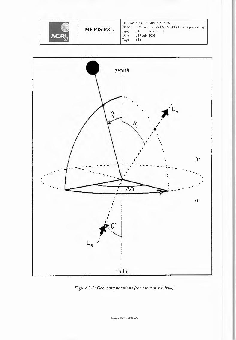
The Geometry notations and conventions in this document are those of RD3. They arerecalled here. In a Cartesian frame linked to the Earth ellipsoid at a given point, the directionsof the Sun and of the observer are represented in figure 2-1 below.
Equations in this document are numbered. The number sequence does not reflect amodel or algorithm logic.
Copyright © 200 I ACRI SA
Doc. No : PO-TN-MEL-GS-0026Name : Reference model for MERIS Level 2 processingIssue : 4 Rev.: IDate : 13 July 200 IPage : 10
MERIS ESL
zenith
,,. ,•,.~';
I
'I
Q+
- ::: - - - - .•. - - -'',
I
I '; - - - - -.-. - - - -- -,- - - - - .,
~,- ..... ...•. .•.• ..•. ..
II o·'I'I
t
~a1 I,r <,, !
nadir
Figure 2-1: Geometry notations (see table of symbols)
Copyright© 2001ACRI S.A.

MERIS ESLDoc.No : PO-TN-MEL-GS-0026Name : Referencemodel for MERISLevel 2 processingIssue : 4 Rev.: IDate : 13July 2001Page : 11
2.5 TABLE OF SYMBOLS
Symbol Dimension I unitsdefinition
Geometry (see fig. 2.1)
..1 Wavelengthes Sun zenith angle (µs = cos(e5))
ev, e Satellite viewing angle(~= cos(ev))
e' Refracted viewing angle (e' = sin-l(n.sin(ev)))
Azimuth difference between the sun-pixel and pixel-sensor
half vertical planes
Scattering angle (not represented)
Radiometric quantitiesL(..1,es,ev,.1¢) Radiance
Inherent Optical Properties ("IOPs"){3(e,..1) volume scattering function (VSF)
{3(e,..1)
a(..1)
b(..1)c(..1)
bb(..1)
normalised volume scattering function
~(0 A.)= ~(0,A.)' b(A.)
where
~(0).)= d<I>(9,A)_I_, <I>0(A)is the radiant flux<I>0 (A) dcodr
onto a volume element of thickness dr, and d<I>(e,A.)ldcois the radiant intensity scattered from this volume in thedirection 0 with respect to the direction of the incidentflux.
Absorption coefficient
Scattering coefficient
Attenuation coefficient for wavelength ..1Backscattering coefficient
Apparent Optical Properties ("AOPs") and derived quantities0..1,es,ev,.1¢) Reflectance (JrLI Ed(0+))1
nmdegrees
degrees
degrees
degrees
degrees
W m-2 nm-I sr !
srl
sr lrrr l
dimensionless
where the product Jr.L is the TOA upwelling irradiance ifupwelling radiances are equal to L(..1,es,ev,.1¢),for any values of ev
within 0-Jr/2 and any .1¢within 0-2Jr.
1 This definition actually corresponds to the transformation of the normalised water-leaving radiance sensuGordon and Clark (1981) (i.e., LI (Ee tes µ5)) into reflectance through the usual equation p = TCLI Fo µ5 (with µ5
= 1 in this last case).Copyright c 200 I ACRI SA
MERIS ESLDoc. No : PO-TN-MEL-GS-0026Name : Reference model for MERIS Level 2 processingIssue : 4 Rev.: IDate : 13 July 2001Page : 12IIc
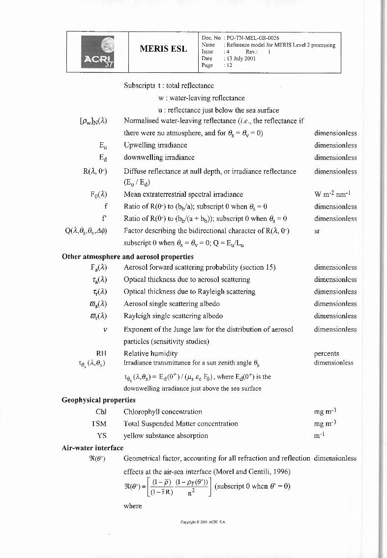
Subscripts t : total reflectance
w : water-leaving reflectance
u : reflectance just below the sea surfaceNormalised water-leaving reflectance (i.e., the reflectance if
there were no atmosphere, and for es = ev = 0)
Upwelling irradiance
downwelling irradiance
Diffuse reflectance at null depth, or irradiance reflectance(Eu I Ed)Mean extraterrestrial spectral irradiance
Ratio of R(O-)to (bb/a); subscript 0 when es = 0Ratio of R(O-)to (bb/(a + bb)); subscript 0 when es= 0
Factor describing the bidirectional character of R(A-,O-)
subscript 0 when es = ev = 0; Q = Eu/Lu
Other atmosphere and aerosol propertiesFa(A) Aerosol forward scattering probability (section 15)
R(A-,O-)
F0(A-)fr
ra(A-)
rr(A-)
CUa(A)
CUr(A-)
Optical thickness due to aerosol scattering
Optical thickness due to Rayleigh scattering
Aerosol single scattering albedo
Rayleigh single scattering albedo
Exponent of the Junge law for the distribution of aerosol
particles (sensitivity studies)
Relative humidityIrradiance transmittance for a sun zenith angle es
v
downwelling irradiance just above the sea surface
Geophysical propertiesChl Chlorophyll concentration
TSM
YS
Total Suspended Matter concentration
yellow substance absorption
dimensionless
dimensionless
dimensionless
dimensionless
Wm-2 nm-I
dimensionless
dimensionless
sr
dimensionless
dimensionless
dimensionless
dimensionless
dimensionless
dimensionless
percentsdimensionless
mgmJ
mg rrr-'rrr !
Air-water interface9\(0') Geometrical factor, accounting for all refraction and reflection dimensionless
effects at the air-sea interface (Morel and Gentili, 1996)
9\(0')= [ (1-_/5) (1- pp(O'))l (subscript 0 when e' = 0)(1-rR) n2
where
Copyright© 2001ACRI S.A.

Doc. No : PO-TN-MEL-GS-0026Name : Reference model for MERIS Level 2 processingIssue : 4 Rev.: 1Date : l3 July 200 lPage : 13
MERIS ESL
n is the refractive index of waterPF( 8) is the Fresnel reflection coefficient for incident
angle ep is the mean reflection coefficient for the downwelling dimensionless
dimensionlessdimensionless
irradiance at the sea surface
r is the average reflection for upwelling irradiance at the dimensionless
water-air interface
a Root-mean square of wave facet slopes dimensionless
f3 Angle between the local normal and the normal to a wave facet
p Probability density of surface slopes for the direction dimensionless(es, ev, .1¢)
MiscellaneousWind speedCorrection factor applied to F0(A..), and
accounting for the changes in the Earth-sun distance.
It is computed from the eccentricity of the Earthorbit, e = 0.0167, and from the day number D, as
,, = (1+e co{2" i~s-J))rIn natural (or Neperian) logarithm
w dimensionlessdimensionless
log10 decimal logarithm
Copyright© 200I ACRI S.A.
MERIS ESLDoc. No : PO-TN-MEL-GS-0026Name : Reference model for MERIS Level 2 processingIssue : 4 Rev.: IDate : 13 July 2001Page : 14
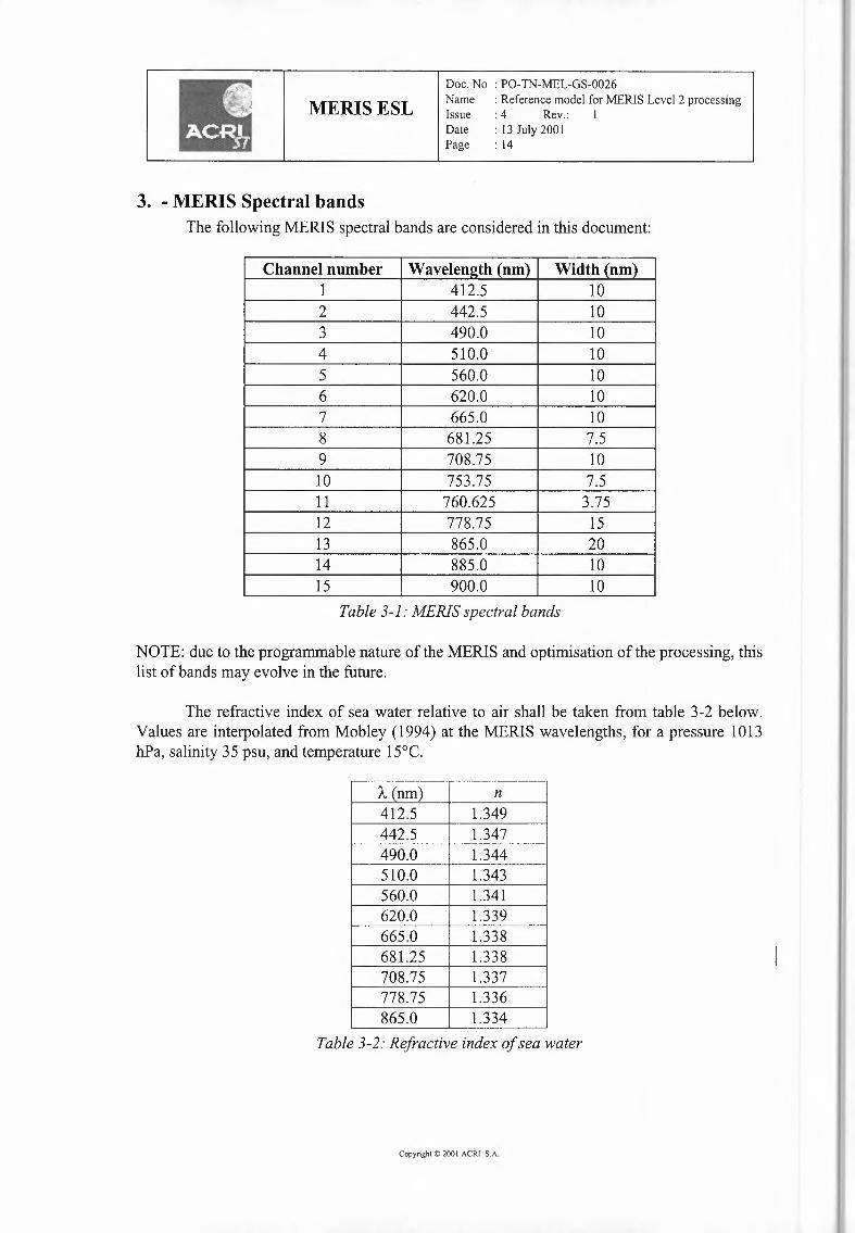
Channel number Wavelength (nm) Width (nm)1 412.5 102 442.5 103 490.0 104 510.0 105 560.0 106 620.0 107 665.0 108 681.25 7.59 708.75 1010 753.75 7.511 760.625 3.7512 778.75 1513 865.0 2014 885.0 1015 900.0 10
3. - MERIS Spectral bandsThe following MERIS spectral bands are considered in this document:
Copyright© 2001ACRI SA
Table 3-1: MERIS spectral bands
NOTE: due to the programmable nature of the MERIS and optimisation of the processing, thislist of bands may evolve in the future.
The refractive index of sea water relative to air shall be taken from table 3-2 below.Values are interpolated from Mobley (1994) at the MERIS wavelengths, for a pressure 1013hPa, salinity 35 psu, and temperature l 5°C.
'A (nm) n412.5 1.349442.5 1.347490.0 1.344510.0 1.343560.0 1.341620.0 1.339665.0 1.338681.25 1.338708.75 1.337778.75 1.336865.0 1.334
Table 3-2: Refractive index of sea water

MERIS ESLDoc. No : PO-TN-MEL-GS-0026Name : Reference model for MERIS Level 2 processingIssue : 4 Rev.: IDate : 13 July 200 IPage : 15
4. - Water Optical PropertiesAt a given A, the optical properties described below apply to Case 1 and Case 2 ocean
waters (tentatively to inland waters). Water optical properties shall be computed at least forthe following MERIS bands:
1, 2, 3, 4, 5, 6, 7, 9, 12, 13 for algorithms which include atmosphere correction;1, 2, 3, 4, 5, 6, 7, 9 for algorithms based on water-leaving radiance (or reflectance)
4.1 - REMOTELY SENSED LAYER
The geometrical thickness of the vertical water layer from which 90% of the remotelysensed ocean colour signal emerges [denoted Z90('A); m] can be approximated by (Gordon andMcCluney 1975):
(la)where Ka(A) (m") is the vertical attenuation coefficient for downward irradiance. Here, weassume that (whatever A.)
z >> Z90(A.) (lb)where z (m) is the geometrical thickness of the water column. In other words, bottom effect isnot accounted for in the present model.
4.2 - WATER CONSTITUENTS
4.2.1 -OVERVIEW
This section presents the concepts and terminology used through the discussion andspecification of the water optical properties models.
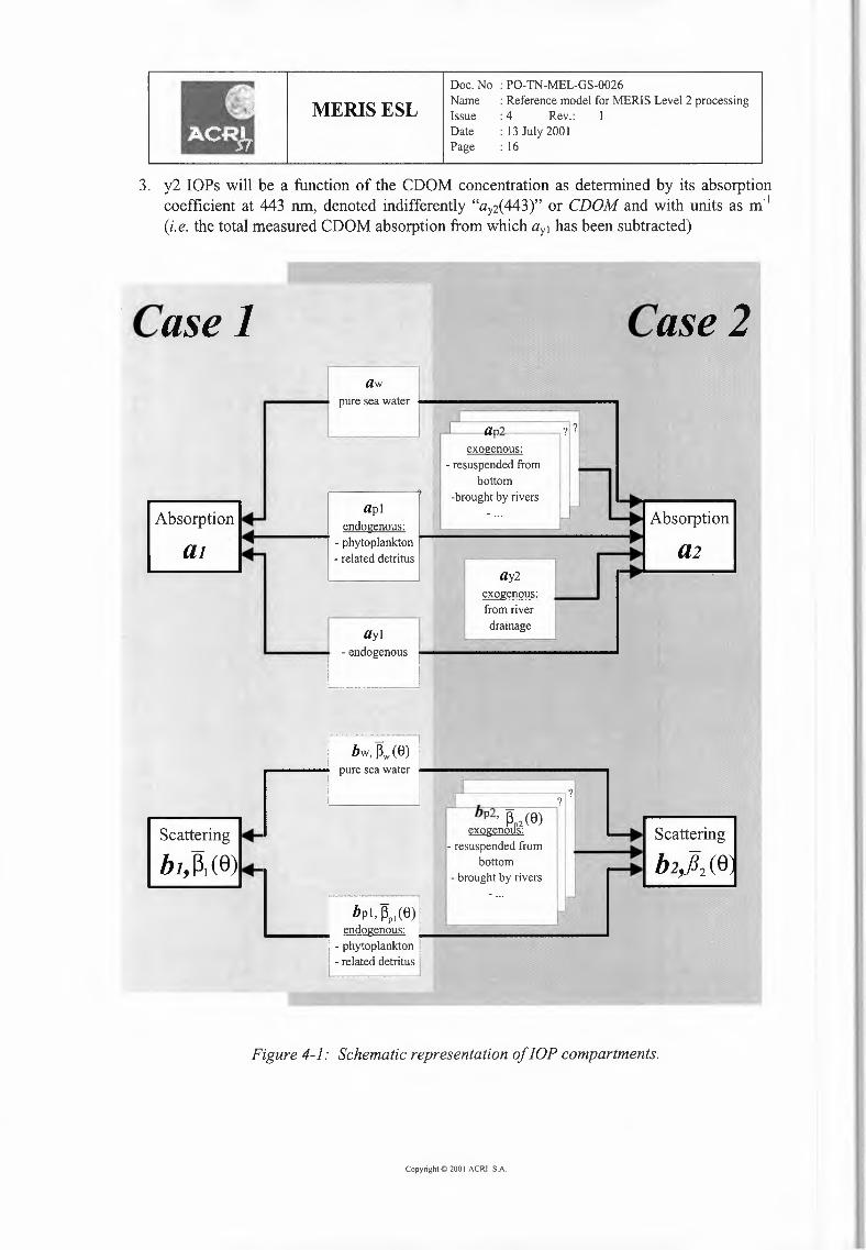
The apparent optical properties of sea waters can be determined according to theinherent optical properties (absorption and scattering) of 5 groups of substances (cf Fig. 4-1):
1. pure sea water, denoted "w"2. phytoplankton and other associated particles (detritus, bacteria, ... ), denoted "pl"3. endogenous coloured dissolved organic matter (associated with biological activity),
denoted "y l"4. terrestrial (exogenous) particles (sediment resuspended from the bottom, brought by
rivers, ... ), denoted "p2"5. exogenous coloured dissolved organic matter from land drainage (present in Case 2
waters only), denoted "y2".
While only groups 1, 2 and 3 are present in Case 1 waters, all of them (1 to 5 above)co-exist in Case 2 waters. In this case, however, the individual components y 1 and y2 cannotbe practically separated (a measure of CDOM absorption provides the sum yl + y2).
IOPs of groups 2, 3, 4 and 5 are related to the following "concentrations":1. pl and yl IOPs will be a function of the concentration of chlorophyll a (including the
divinyl form and pheopigments) denoted "[ch!}" and with units as mg m-32. p2 IOPs will be ideally related to the sea water particles dry weight (denoted "TSM' and
with units as g m") from which the contribution of pl has been subtracted; practically it isrelated to the corresponding scattering coefficient (units m-1).
Copyright © 200 I ACRI S.A.
MERIS ESLDoc. No : PO-TN-MEL-GS-0026Name : Reference model for MERIS Level 2 processingIssue : 4 Rev.: 1Date : 13 July 2001Page : 16
3. y2 IOPs will be a function of the CDOM concentration as determined by its absorptioncoefficient at 443 run, denoted indifferently "ay2(443)" or CDOM and with units as m·1(i.e. the total measured CDOM absorption from which ay1 has been subtracted)
Case]
Absorption
Casei2aw
pure sea water
llpl
llp2---exogenous:
- resuspended frombottom
-brought
Absorption
a1endogenous: II• I - phytoplankton ....,
- related detritus a2
Scattering
b1,P1 (8)
llyl____ .,., - endogenous
lly2exogenous:from riverdrainage
pure sea water
bp1, 13p1(8) Iendogenous: .' __.__.__. _
- phytoplankton- related detritus
?
bp2, l3 2 (8) ,·exogenoil's:
- resuspended frombottom
- brought by rivers
Scattering
b2,f32 (8
Figure 4-1: Schematic representation of !OP compartments.
CopyrightO 200I ACRI SA

Doc. No : PO-TN-MEL-GS-0026Name : Reference model for MERIS Level 2 processingIssue : 4 Rev.: IDate : 13 July 200 IPage : 17
MERIS ESL
Comments on Figure 4-1
Case 2 waters are seen as Case 1 waters to which other optically active substances areadded. In other words, Case 1 waters can be seen as particular Case 2 waters whenthese additional substances are lacking.
Case 1 waters include 3 components:pure sea water for which 2 spectral IOPs must be specified: aw(A)and f3w(A,()); this lastterm can be split into "j3w(8) (independent from A) and bw(A)all particulate matter found in open ocean, such as living algal cells, heterotrophicbacteria and organisms, various debris, ... Again, this compartment is described by itsabsorption and scattering properties: apJ(A),bp1(A)and "j3pl (8)coloured dissolved organic material presumably generated in open ocean (throughprocesses like excretion, organism decay, .. .), and likely related to the particulatematter abundance. This compartment comes into play through its absorption coefficientayi(A,)In summary, there are 3 components informing the absorption coefficient of Case 1waters and 2 components in forming the scattering properties.
Case 2 waters include the three above components and in addition:exogenous particles, mainly sediment, either transported by rivers, or re-suspendedfrom the bottom in shallow waters. The proportions between organic and mineralparticles is varying according to the location and origin; the mineral particles are alsogeographically differing (clay, calcareous, .. .). Therefore, several types of particlesmay be simultaneously present, and to each type corresponds a couple of properties likeap2(A) and /3p2(A,())exogenous CDOM resulting from land drainage which acts only as absorber: ay2(A). Asfor particles, it is likely that several types may be distinguished depending on thelocation.
4.2.2 - RELATIONSHIP WITH MERIS LEVEL 2 PRODUCTS
The way the IOPs presented above will be practically related to the MERIS Level 2products is explained separately for Case 1 and Case 2 waters in sections 4.5 and 4.6 below,respectively.
To summarise:
• The Algal Pigment Index 1 product corresponds to PI (and take YI into account), inCase 1 waters.
• The Algal Pigment Index 2 product corresponds to the absorption of PI·• The Total Suspended Matter product corresponds to the aggregate scattering of pl and
p2.• The Yellow Substance product corresponds to the aggregate absorption of p2, YI and
Y2·
Copyright© 200I ACRI S.A.
MERIS ESLDoc. No : PO-TN-MEL-GS-0026Name : Reference model for MERIS Level 2 processingIssue : 4 Rev.: 1Date : 13 July 2001Page : 18
4.3 - VERTICAL DISTRIBUTION
It is assumed that all substances are homogeneously distributed in the upper part of thewater column. For many coastal waters, this is a realistic assumption, especially whenconsidering the Z90(A.)layer; this may be false for river plumes, where very strong verticalgradients associated with fresh water spreading may be observed.
4.4 INHERENT OPTICAL PROPERTIES (IOPS) OF PURE SEA WATER
These Inherent Optical Properties are involved in both Case 1 and Case 2 waters andinclude absorption, scattering, and emission (Raman) properties.
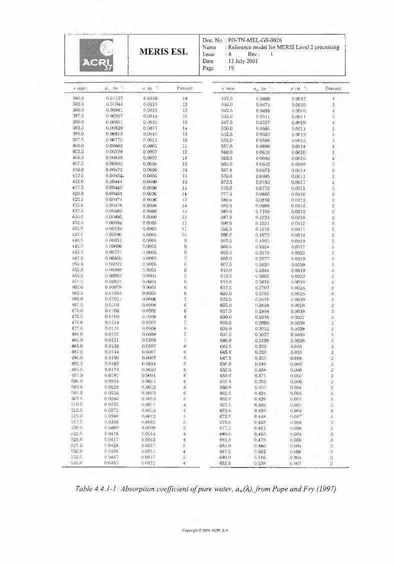
4.4.1 ABSORPTION COEFFICIENT
The absorption coefficients of pure sea water, aw (ll), are taken from Pope and Fry(1997) for wavelengths up to 709 nm, i.e. up to and including MERIS band 9, and from Haleand Querry (1973) for wavelengths above 709nm (see Table 4.4.1-1 below).
Copyright© 2001ACRI S.A.
MERIS ESL
Percent
Doc. No : PO-TN-MEL-GS-0026NameIssueDatePage
: Reference model for MERIS Level 2 processing: 4 Rev.: 1: 13 July 2001: 19
380J)382.5,J&:i.O387.J;:l!!O.O392.5:195.0;397 5400.04D2.5406.0407.i\~10.fl412.t~415.04l7.5·l20.0422.5425.0
.1.%.0-l:tT.544{),(l
44i.S44.'».0Hi.Ci450.0452._r)455.0
4601)462.546.5.0·167.5470.0472.547!..(I
41\fd)41\7.5490.0492.5·t9.'>.0·197.:;ri(j().(l
f>(l'25SOC•0:)07 f1.'.:·10{1;)-12.!1sis.o
5:W.O
5:lii.O
0.01137O.CH04.4IUJ()!l4l(I 00917O.Oc.551OJJ0829O.OOS130.007750.0006.~(},(>!)519o.(~J5:Jo(L(1':)503O.OQ47Jll0045'.il{J.0Q.l440.004420.0(14,'i40.0(1414(J.()!)47$()(){)~
()(){)495
IH}()5(40 <XJ5300.00.5800.00635n.oosss0.0075!0.00S!'J.O0.()09'.tZ0.(){J!#>'"\!()(){)%2f)[J<)96''700<)B790.010050.0101l0.0Hl20.0106{).fJ!09o 0114O.()IZlO.GJ270.01310.f}1360.01440.01500-°1£20.(Jl'i':)o.ornrO.OW'10,022.S0.0200() 028£>0032(}0..0~172o.n:NnU1):li!9D.040!)0.0416O.O·ll70.04280.•M340.fl-447(}.IM.52
o.onu;1.100150.0011OJ.!01'10.0012O.(M>ll0.tJo:)l(IOOOllnOOOIGJl0070.00070.00060.00000.0CIOblHi!lOo0.(1'000(U10060.00060.0006uooesD.0006O.OOOf>0.0{105O.OfJ050.()()(150.0005OJ)OOGo.ooos()J)(KJ5l)J)•J().i{1_0004D.00040.000..'\0.01'.H'.J;~0.(!ll:~)j_iO.lil(Hl6O.(K)l)50.00080.00070.0008(1.00080.00080.00070.00070.0007O.(i.J140,001(1O.OQHO.CIOUOJJ(ll2uneiaO.fJOJt)H.!Jl1l l0.00120.{)()120.(){)!5
(l ()()09
CHKH40.0010O.Of)l 70.0011fJ(l(f] ill.0012
14is1316Iii1413is11121413is1313HH13l•l1312ull10H98
B6
7H68
,,..,.66596866I)
44453·i4
a. cm 11 o im 11
5!37.5r,4(LOt.425545.0647.56M.O55.2.5sss.o557.t.560.0ssz.e:.65.0Ml7.5570 ..0572.5571).0fi'ri.5511().()
585.0,')87 .5590.0S92.5[•95.0ftH7"5600.f)602.56(~">.()607.~=t610.<J612.5fjJ:),(I
617.5620.0622.5625.06271)63-0.06:{2,5f:i;l.~.oGa7.5&10.0642.51)45.(l64:7Jj650.!)6!i2.!·6.'i!>.065751)6(),(l662.5665.0667.fimo.o~;72.11675.0i".'.!<"T"' rUI J • .,)
fiii.I),()1%2.iiess.o1!87.669Cf.O692!1
lU)-466(l.fJoi740.04890.05110.0537fJ.05tk'to.o5fK~0.059'60.00000.06190.004.(1O.Of.42(l.0672(l.(J6950.07330.()772O.OSIJ'60.08000.0089o.noo().1220O.l:lSJ(f.1516O.l6i20.19'2!1ll.2:.144U.24700.'2577026W0.2&H0.2'661i0.26780..27{!70.2755(L21)Hl(l.2S.:.t4(1,29':'40.2916IJ.29960.30120.3-0770.31080.3220.32.S0.33.,",()~'340u.~~58,o.,n1O;J."!J:J0.1 to0.4.240.·129o.·ta6<t·1a1i0441'0.44.'<(1.41310.4650,478O.·IS60.502o.srs0.53S
0.00150.00100.0016(L00ll(L(l(lJ!iunon1.1.001.2U.lJ0120.00140.0010uocis(l.()0090.0(ll4O.OOil0.00H000110.0016G.00120.00160.1)0120.00180.(){)12().(){)17
0,(){)14
0.0919(),0017OJJ0230.0019O.f.l(Y.MlOJXtlllO.fJ0230.{)()19
i)OO~!iOl)(J2f>~wo:m0.00280.00390.0027G.00380..00280.0M!l0.002fi0.0050.003(),(){!4().(HJ:)(),(M)60.0<.130.0060.0!140.005OJ)(Hn.ooc.0.()1)4(l/;()70()()40.006U004O.OOC,O.OCHD.OOii0,fJ()4{){)(17
3
,,d
3333
Table 4.4.1-1: Absorption coefficient of pure water, aw(A),from Pope and Fry (1997)
Copyright© 2001ACRI S.A.
Doc. No : PO-TN-MEL-GS-0026Name : Reference model for MERIS Level 2 processingIssue : 4 Rev.: 1Date : 13 July 2001Page : 20
33333333333333
MERIS ESL
A.(nm)
695.0697.5700.0702.5705.0707.5710.0712.5715.0717.5720.0722..5725.0727.5
0.6590.6920.6240.6630!1040.7560.827o.9141.0011.119L2311.3561.4891.678
OJXl50.0080.1)060.0080.0060.0090.0070.0110.0090.0140.0110.0080.0060.007
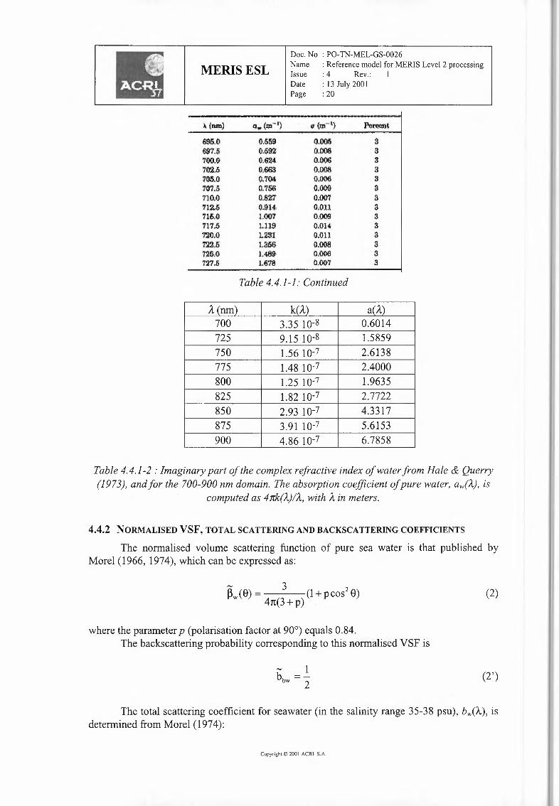
Table 4.4.1-1: Continued
/l (nm) k(/l) a(/l)700 3.35 10-8 0.6014725 9.15 10-8 1.5859750 1.56 10-7 2.6138775 1.48 10-7 2.4000800 1.25 10-7 1.9635825 1.82 10-7 2.7722850 2.93 10-7 4.3317875 3.91 10-7 5.6153900 4.86 10-7 6.7858
Table 4.4.1-2: Imaginary part of the complex refractive index of water from Hale & Querry(1973), and for the 700-900 nm domain. The absorption coefficient of pure water, aw(ll), is
computed as 4-nk(/l)IA.,with /l in meters.
4.4.2 NORMALISED VSF, TOTAL SCATTERING AND BACKSCATTERING COEFFICIENTS
The normalised volume scattering function of pure sea water is that published byMorel (1966, 1974), which can be expressed as:
- 3~w(S)= (l+pcos28)47t(3+p)
(2)
where the parameter p (polarisation factor at 90°) equals 0.84.The backscattering probability corresponding to this normalised VSF is
(2')
The total scattering coefficient for seawater (in the salinity range 35-38 psu), bw(A), isdetermined from Morel (1974):
Copyright© 200I ACRI S.A.
MERIS ESLDoc.No : PO-TN-MEL-GS-0026Name :ReferencemodelforMERISLevel2processingIssue : 4 Rev.: 1Date : 13July2001Page : 21
(A, )-4.32
bw(A-) = 0.00288. -500
(3)
Note that for freshwater it is
(A, J-4.32
bw(A) = 0.00222. -500
(3')
Note that the variation of b., with salinity is roughly a linear function of salinity.
4.4.3 EMISSION
See section 4.5.4.1
4.5 CASE 1WATERS IOPs
4.5.1 TOTAL ABSORPTION COEFFICIENT (PURE SEA WATER AND PHYTOPLANKTON2)
Here, the analytical approach suggested by Fig. 4.1, and which consists of explicitlymodelling a1 as the sum [aw + apl + ayi] is not used, by lack of knowledge of a stablerelationship (if any) between [Chi] and the associated endogenous yellow substance. Theindirect approach used here rests on the consideration of Kd(/...). Indeed, this coefficient mergesthe influences of all absorbing substances, without discriminating their separate contributions.Therefore a1 is globally determined as a function of [Chi] as described in Morel andMaritorena (2000)
(8)
where Kd(/...) is given as a function of [chi] (see table 4.5.1-1 below):
(9)
The factor u is determined by iterations as described in Morel ( 1988) and Morel andMaritorena (2000). This scheme consists of introducing bb(A) in the following equation
(10)
where R is the irradiance reflectance (Eu I Ed), and bb = bbw + bbp 1. The coefficient bbw iscalculated according to Eqs. (2') and (3) above, and bbpl according to Eq. (18) below(§4.5.2.2). Then a1(A.) is replaced by u, Kd(A.), with u, = 0.75, whatever the wavelength and fis set to 0.33. A first set of R(A.)values is thus derived. Then, an exact relationship (derivedfrom the Gershun's equation), namely
01) I
2 Here, "phytoplankton" means the livingalgal cells as well as all other particulateor dissolvedmatter found inopen ocean, such as heterotrophic bacteria and organisms, various debris, yellow substances etc.... (seecommentson Fig.4.1).
Copyright© 200I ACRI S.A.

MERIS ESLDoc. No : PO-TN-MEL-GS-0026Name : Reference model for MERIS Level 2 processingIssue : 4 Rev.: IDate : 13 July 2001Page : 22
is operated by letting µu equal to 0.42, by interpolating u, from the values given in table 4.5.1-2 below as a function of the chlorophyll concentration and wavelength, and by neglectingdR/dZ, which results in
a1(A.)= Kt(A.)~ [I + (µ<l /0.42) R(A.)]-1 [I - R(A.)] (11 ')or
(11")
The first set of R(A.) values is used to produce the spectrally varying u2(A.)values throughEq .11' and a new set of a1(A.)values through Eq. 11''. The value of a1 shall be constrained tobe higher than or equal to aw(A.)(from §4.4.1 above). With these adjusted a1(A.)values,through a second loop using Eq. (10), a more accurate set of R(A.)values is derived, and soforth. Stable R(A.)values (then stable a1(A.)values) are obtained within three loops in thisiterative process. The final a1(A.)values are given in Table 4.5.1-3.
Copyright <O200 I ACRI S.A.
MERIS ESLDoc. No : PO-TN-MEL-GS-0026Name : Reference model for MERIS Level 2 processingIssue : 4 Rev.: IDate : 13 July 200 IPage : 23
/.... Kw e x /.... Kw e x /....(nm) a(/....)(m-1)
350 0.02710 0.77800 0.15300 530 0.04454 0.67224 0.04829 775 2.400355 0.02380 0.76700 0.14900 535 0.04630 0.66739 0.04611 800 1.963360 0.02160 0.75600 0.14400 540 0.04846 0.66195 0.04419 825 2.772365 0.01880 0.73700 0.14000 545 0.05212 0.65591 0.04253 850 4.331370 0.01770 0.72000 0.13600 550 0.05746 0.64927 0.04111 875 5.615375 0.01595 0.70000 0.13100 555 0.06053 0.64204 0.03996 900 6.786380 0.01510 0.68500 0.12700 560 0.06280 0.64000 0.03900385 0.01376 0.67300 0.12300 565 0.06507 0.63000 0.03750390 0.01271 0.67000 0.11900 570 0.07034 0.62300 0.03600395 0.01208 0.66000 0.11800 575 0.07801 0.61500 0.03400400 0.01042 0.64358 0.11748 580 0.09038 0.61000 0.03300405 0.00890 0.64776 0.12066 585 0.11076 0.61400 0.03280410 0.00812 0.65175 0.12259 590 0.13584 0.61800 0.03250415 0.00765 0.65555 0.12326 595 0.16792 0.62200 0.03300420 0.00758 0.65917 0.12269 600 0.22310 0.62600 0.03400425 0.00768 0.66259 0.12086 605 0.25838 0.63000 0.03500430 0.00770 0.66583 0.11779 610 0.26506 0.63400 0.03600435 0.00792 0.66889 0.11372 615 0.26843 0.63800 0.03750440 0.00885 0.67175 0.10963 620 0.27612 0.64200 0.03850445 0.00990 0.67443 0.10560 625 0.28400 0.64700 0.04000450 0.01148 0.67692 0.10165 630 0.29218 0.65300 0.04200455 0.01182 0.67923 0.09776 635 0.30176 0.65800 0.04300460 0.01188 0.68134 0.09393 640 0.31134 0.66300 0.04400465 0.01211 0.68327 0.09018 645 0.32553 0.66700 0.04450470 0.01251 0.68501 0.08649 650 0.34052 0.67200 0.04500475 0.01320 0.68657 0.08287 655 0.37150 0.67700 0.04600480 0.01444 0.68794 0.07932 660 0.41048 0.68200 0.04750485 0.01526 0.68903 0.07584 665 0.42947 0.68700 0.04900490 0.01660 0.68955 0.07242 670 0.43946 0.69500 0.05150495 0.01885 0.68947 0.06907 675 0.44844 0.69700 0.05200500 0.02188 0.68880 0.06579 680 0.46543 0.69300 0.05050505 0.02701 0.68753 0.06257 685 0.48642 0.66500 0.04400510 0.03385 0.68567 0.05943 690 0.51640 0.64000 0.03900515 0.04090 0.68320 0.05635 695 0.55939 0.62000 0.03400520 0.04214 0.68015 0.05341 700 0.62438 0.60000 0.03000525 0.04287 0.67649 0.05072 705 0.74200 0.60000 0.02500
710 0.83400 0.60000 0.02000715 1.00200 0.60000 0.01500720 1.17000 0.60000 0.01000725 1.48500 0.60000 0.00700730 1.80000 0.60000 0.00500735 2.09000 0.60000 0.00200740 2.38000 0.60000 0.00000745 2.42000 0.60000 0.00000750 2.47000 0.60000 0.00000
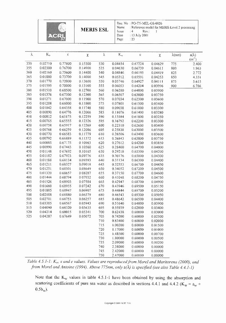
Table 4.5.1-1: Kw,x and e values. Values are reproduced from Morel and Maritorena (2000), andfrom Morel and Antoine (1994). Above 775nm, only a(A.) is specified (see also Table 4.4.1-1)
Note that the Kw values in table 4.5.1-1 have been obtained by using the absorption andscattering coefficients of pure sea water as described in sections 4.4.1 and 4.4.2 (Kw = ~ +0.5bw)-
Copyright© 200I ACRI S.A.
Doc. No : PO-TN-MEL-GS-0026Name : Reference model for MERIS Level 2 processingIssue : 4 Rev.: IDate : 13 July 2001Page : 24•- MERIS ESL
0.03 0.1 0.3 1. 3. 10.350. 0.770 0.769 0.766 0.767 0.767 0.767400. 0.770 0.769 0.766 0.767 0.767 0.767412. 0.765 0.770 0.774 0.779 0.782 0.782443. 0.800 0.797 0.796 0.797 0.799 0.799490. 0.841 0.824 0.808 0.797 0.791 0.791510. 0.872 0.855 0.834 0.811 0.796 0.796555. 0.892 0.879 0.858 0.827 0.795 0.795620. 0.911 0.908 0.902 0.890 0.871 0.871670. 0.914 0.912 0.909 0.901 0.890 0.890700. 0.914 0.912 0.909 0.901 0.890 0.890710. 0.914 0.912 0.909 0.901 0.890 0.890
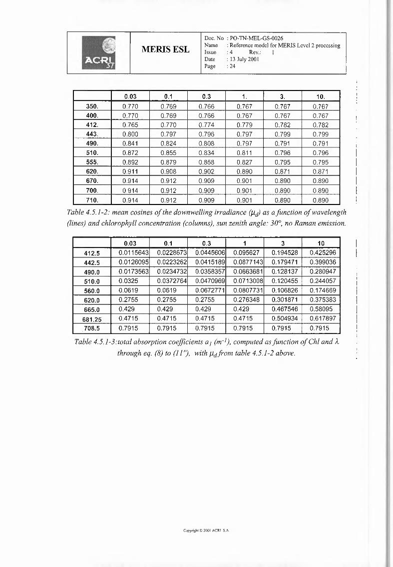
Table 4.5.1-2: mean cosines of the downwelling irradiance (µcJ)as afunction of wavelength(lines) and chlorophyll concentration (columns), sun zenith angle: 30°, no Raman emission.
0.03 0.1 0.3 1 3 10412.5 0.0115643 0.0228673 0.0445606 0.095627 0.194528 0.425296
442.5 0.0126095 0.0223262 0.0415189 0.0877143 0.179471 0.399036
490.0 0.0173563 0.0234732 0.0358357 0.0663681 0.128137 0.280947510.0 0.0325 0.0372764 0.0470969 0.0713008 0.120455 0.244057
560.0 0.0619 0.0619 0.0672771 0.0807731 0.106826 0.174669
620.0 0.2755 0.2755 0.2755 0.276348 0.301871 0.375383665.0 0.429 0.429 0.429 0.429 0.467546 0.58095
681.25 0.4715 0.4715 0.4715 0.4715 0.504934 0.617897708.5 0.7915 0.7915 0.7915 0.7915 0.7915 0.7915
Table 4.5.l-3:total absorption coefficients a1 (m:l}, computed as function ofChl and Athrough eq. (8) to (I I"), with µdfrom table 4.5.1-2 above.
Copyright© 200I ACRI S.A.

MERIS ESLDoc. No : PO-TN-MEL-GS-0026Name : Reference model for MERIS Level 2 processingIssue : 4 Rev.: 1Date : 13 July 2001Page : 25
4.5.2 NORMALISED VSF, TOTAL SCATTERING, AND BACKSCATTERING COEFFICIENTS
4.5.2.1 Pure Sea WaterSee section 4.4 above.
4.5.2.2 Case 1 Waters Particles (phytoplankton and its retinue)The normalised VSF for Case 1 waters particles is obtained as a mixture of two
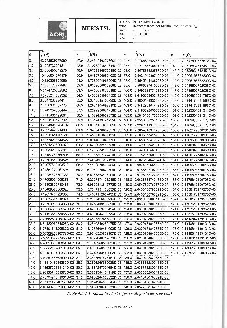
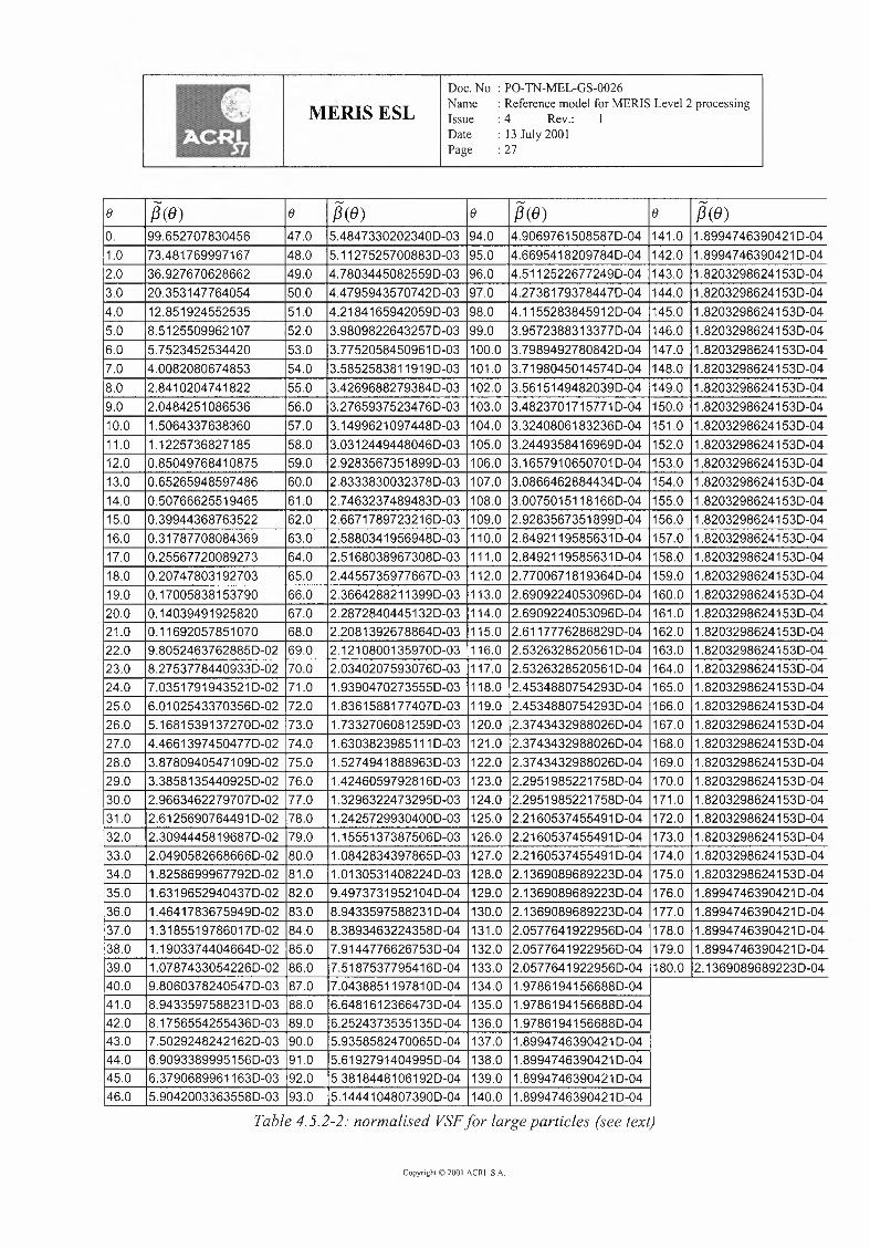
separately computed VSFs (Fig. 4.2). The first one (Table 4.5.2-1) corresponds to apopulation of "small" non-absorbing particles of spheroidal shape, with a relative index ofrefraction equal to 1.06, and assumed to obey a Junge law with the exponent set equal to -4.2.The second population corresponding to "large" particles (Table 4.5.2-2) is identical exceptthat the Junge exponent is equal to -3. The weighted sum of these two VSFs provides
- - -,BP1(8,Chl) = w,(Chl) ,Bp1,,(8) + w1(Chl) ,Bp1,1(8) (12)
where the subscripts s and 1 stand for small and large particles, respectively, and where theweights ws and w1are such that :
w8(Chl) + w1(Chl)= 1 (13)
Vv's(Chl)= 0.855 (0.5 - 0.25 log10(Chl)) (14)
The normalised VSF computed through Eq. (12) are assumed to be wavelengthindependent (no change in shape).
The backscattering efficiency for Case 1 water particles that derives from the use ofthe above chlorophyll-varying normalised VSF exactly matches the following expression(from Morel and Maritorena, 2000) :
bbr1(A) = 0.002+ [0.01 [0.5-0.25log10(chl)]] (15)
At 550 nm, the particle scattering coefficient, bp1(550), is taken from Loisel and Morel(1998):
(16)
where AbpJ and Bbpl equal 0.416 and 0.766, respectively. The factor of variation in AbpI equals1.3.
CopyrightCO 2001ACRI S.A.
MERIS ESLDoc. No : PO-TN-MEL-GS-0026Name : Reference model for MERIS Level 2 processingIssue : 4 Rev.: IDate : 13 July 2001Page : 26
e f3(8) e /3(8) e /3(8) e /3(8)0. 42.282829537580 47.0 2.24515162773600-02 94.0 2.77668929225300-03 141.0 2.05475007626720-031.0 34.958732391211 48.0 2.10235046413440-02 95.0 2.72115550640790-03 142.0 2.06268347424510-032.0 23.065450213275 49.0 1.97065605770180-02 96.0 2.65768832258500-03 143.0 2.06268347424510-033.0 15.40680167 4179 50.0 1.84927506864050-02 97.0 2.6021545367 4000-03 144.0 2.07061687222300-034.0 10.720368953898 51.0 1.738207 49695040-02 98.0 2.55455414887280-03 145.0 2.07061687222300-035.0 7.6237177877997 52.0 1.63586666303590-02 99.0 2.50695376100560-03 146.0 2.07855027020080-036.0 5.5174720252582 53.0 1.54066588730150-02 100.0 2.45935337313840-03 147.0 2.07855027020080-037.0 4.0755214089952 54.0 1.45339850954500-02 101.0 2.41968638324900-03 148.0 2.08648366817870-038.0 3.0647033724414 55.0 1.37168451037300-02 102.0 2.38001939335970-03 149.0 2.09441706615660-039.0 2.3450331082773 56.0 1.29711056938100-02 103.0 2.34828580144830-03 150.0 2.09441706615660-0310.0 1.8249354036444 57.0 1.22729666717580-02 104.0 2.31655220953680-03 151.0 2.10235046413440-0311.0 1.4415460129661 58.0 1.16224280375730-02 105.0 2.28481861762530-03 152.0 2.10235046413440-0312.0 1.1551186123732 59.0 1.10194897912550-02 106.0 2.25308502571390-03 153.0 2.11028386211230-0313.0 0.93748963904439 60.0 1.04641519328050-02 107.0 2.22928483178030-03 154.0 2.11028386211230-0314.0 0.76994420714985 61.0 9.94054766626570-03 108.0 2.20548463784670-03 155.0 2.11821726009010-0315.0 0.63911454109686 62.0 9.4566103896159 0-03 109.0 2.18961784189090-03 156.0 2.11821726009010-0316.0 0.5357 4236544527 63.0 9.00440670487760-03 110.0 2.16581764 795730-03 157.0 2.12615065806800-0317.0 0.45312395890378 64.0 8.57600321407280-03 111.0 2.14995085200160-03 158.0 2.13408405604590-0318.0 0.38633268132813 65.0 8.17933331517960-03 112.0 2.13408405604590-03 159.0 2.13408405604590-0319.0 0.33187783760806 66.0 7.79853021224200-03 113.0 2.11821726009010-03 160.0 2.142017 45402370-0320.0 0.28700653864525 67.0 7.44946070121590-03 114.0 2.10235046413440-03 161.0 2.142017 45402370-0321.0 0.24977510193512 68.0 7.11625798614560-03 115.0 2.09441706615660-03 162.0 2.14995085200160-0322.0 0.21861271467807 69.0 6.79892206703090-03 116.0 2.07855027020080-03 163.0 2.14995085200160-0323.0 0.19234523397335 70.0 6.50538634184990-03 117.0 2.07061687222300-03 164.0 2.14995085200160-0324.0 0.17006031905353 71.0 6.227717 41262460-03 118.0 2.06268347424510-03 165.0 2.15788424997950-0325.0 0.15102809730463 72.0 5.95798188137720-03 119.0 2.0547500762672 0-03 166.0 2.15788424997950-0326.0 0.13469323086820 73.0 5.70411314608550-03 120.0 2.04681667828940-03 167.0 2.16581764 795730-0327.0 0.12058764926356 74.0 5.46611120674950-03 121.0 2.04681667828940-03 168.0 2.16581764795730-0328.0 0.10834641618371 75.0 5.23604266539140-03 122.0 2.03888328031150-03 169.0 2.16581764795730-0329.0 9.76759959034830-02 76.0 5.02184091998900-03 123.0 2.03888328031150-03 170.0 2.17375104593520-0330.0 8.83304530855570-02 77.0 4.82350597054240-03 124.0 2.03094988233360-03 171.0 2.17375104593520-0331.0 8.01193861784660-02 78.0 4.63310441907360-03 125.0 2.03094988233360-03 172.0 2.17375104593520-0332.0 7.28682604266970-02 79.0 4.45063626558270-03 126.0 2.03094988233360-03 173.0 2.18168444391310-0333.0 6.64422080646250-02 80.0 4.28403490804 750-03 127.0 2.02301648435580-03 174.0 2.18168444391310-0334.0 6.07301615205620-02 81.0 4.12536694849020-03 128.0 2.02301648435580-03 175.0 2.18168444391310-0335.0 5.56369200187720-02 82.0 3.97463238691070-03 129.0 2.02301648435580-03 176.0 2.18168444391310-0336.0 5.1091082977 4550-02 83.0 3.83976462128700-03 130.0 2.02301648435580-03 177.0 2.18168444391310-0337.0 4.70053830188540-02 84.0 3.70489685566330-03 131.0 2.03094988233360-03 178.0 2.18961784189090-0338.0 4.33322197551030-02 85.0 3.58589588599530-03 132.0 2.03094988233360-03 179.0 2.18961784189090-0339.0 4.0016059400355 0-02 86.0 3.47482831430520-03 133.0 2.03094988233360-03 180.0 2.19755123986880-0340.0 3.70251683626990-02 87.0 3.36376074261510-03 134.0 2.03094988233360-0341.0 3.43119462542690-02 88.0 3.26062656890280-03 135.0 2.03888328031150-0342.0 3.18525928811310-02 89.0 3.16542579316840-03 136.0 2.03888328031150-0343.0 2.961537 46513730-02 90.0 3.07815841541190-03 137.0 2.03888328031150-0344.0 2.75764913710610-02 91.0 2.99882443563320-03 138.0 2.04681667828940-0345.0 2.57121428462630-02 92.0 2.91949045585460-03 139.0 2.04681667828940-0346.0 2.40143956790000-02 93.0 2.84808987 40538 0-03 140.0 2.05475007626720-03
Table 4.5.2-1: normalised VSFfor small particles (see text)
Copyright© 200I ACRI S.A.
MERIS ESLDoc. No : PO-TN-MEL-GS-0026Name : Reference model for MERIS Level 2 processingIssue : 4 Rev.: 1Date : 13 July 200 IPage : 27
e {3(8) e {3(8) e {3(8) e {3(8)0. 99.652707830456 47.0 5.48473302023400-03 94.0 4.90697615085870-04 141.0 1.8994 7463904210-041.0 73.481769997167 48.0 5.11275257008830-03 95.0 4.66954182097840-04 142.0 1.89947463904210-042.0 36.927670628662 49.0 4.78034450825590-03 96.0 4.51125226772490-04 143.0 1.82032986241530-043.0 20.353147764054 50.0 4.47959435707 420-03 97.0 4.273817937844 70-04 144.0 1.82032986241530-044.0 12.851924552535 51.0 4.21841659420590-03 98.0 4.11552838459120-04 145.0 1.82032986241530-045.0 8.5125509962107 52.0 3.98098226432570-03 99.0 3.95723883133770-04 146.0 1.82032986241530-046.0 5.7523452534420 53.0 3.77520584509610-03 100.0 3.79894927808420-04 147.0 1.82032986241530-047.0 4.008208067 4853 54.0 3.58525838119190-03 101.0 3.71980450145740-04 148.0 1.82032986241530-048.0 2.8410204 741822 55.0 3.42696882793840-03 102.0 3.56151494820390-04 149.0 1.82032986241530-049.0 2.0484251086536 56.0 3.27659375234 760-03 103.0 3.48237017157710-04 150.0 1.82032986241530-0410.0 1.5064337638360 57.0 3.1499621097 4480-03 104.0 3.32408061832360-04 151.0 1.82032986241530-0411.0 1.1225736827185 58.0 3.03124494480460-03 105.0 3.24493584169690-04 152.0 1.82032986241530-0412.0 0.85049768410875 59.0 2.92835673518990-03 106.0 3.16579106507010-04 153.0 1.82032986241530-0413.0 0.65265948597486 60.0 2.83338300323780-03 107.0 3.08664628844340-04 154.0 1.82032986241530-0414.0 0.50766625519465 61.0 2.7463237 4894830-03 108.0 3.00750151181660-04 155.0 1.82032986241530-0415.0 0.39944368763522 62.0 2.66717897232160-03 109.0 2.92835673518990-04 156.0 1.82032986241530-0416.0 0.31787708084369 63.0 2.58803419569480-03 110.0 2.84921195856310-04 157.0 1.82032986241530-0417.0 0.25567720089273 64.0 2.51680389673080-03 111.0 2.8492119585631 0-04 158.0 1.82032986241530-0418.0 0.207 47803192703 65.0 2.44557359776670-03 112.0 2.77006718193640-04 159.0 1.82032986241530-0419.0 0.17005838153790 66.0 2.36642882113990-03 113.0 2.69092240530960-04 160.0 1.82032986241530-0420.0 0.14039491925820 67.0 2.28728404451320-03 114.0 2.69092240530960-04 161.0 1.82032986241530-0421.0 0.11692057851070 68.0 2.20813926788640-03 115.0 2.61177762868290-04 162.0 1.82032986241530-0422.0 9.80524637628850-02 69.0 2.12108001359700-03 116.0 2.53263285205610-04 163.0 1.82032986241530-0423.0 8.27537784409330-02 70.0 2.03402075930760-03 117.0 2.53263285205610-04 164.0 1.82032986241530-0424.0 7.03517919435210-02 71.0 1.93904702735550-03 118.0 2.45348807542930-04 165.0 1.82032986241530-0425.0 6.01025433703560-02 72.0 1.8361588177 4070-03 119.0 2.45348807542930-04 166.0 1.82032986241530-0426.0 5.16815391372700-02 73.0 1.73327060812590-03 120.0 2.37434329880260-04 167.0 1.82032986241530-0427.0 4.46613974504770-02 74.0 1.63038239851110-03 121.0 2.37434329880260-04 168.0 1.82032986241530-0428.0 3.87809405471090-02 75.0 1.52749418889630-03 122.0 2.37434329880260-04 169.0 1.82032986241530-0429.0 3.38581354409250-02 76.0 1.42460597928160-03 123.0 2.29519852217580-04 170.0 1.82032986241530-0430.0 2.96634622797070-02 77.0 1.32963224 732950-03 124.0 2.29519852217580-04 171.0 1.82032986241530-0431.0 2.61256907644910-02 78.0 1.24257299304000-03 125.0 2.21605374554910-04 172.0 1.82032986241530-0432.0 2.30944458196870-02 79.0 1.15551373875060-03 126.0 2.21605374554910-04 173.0 1.82032986241530-0433.0 2.0490582668666 0-02 80.0 1.08428343978650-03 127.0 2.21605374554910-04 174.0 1.82032986241530-0434.0 1.82586999677920-02 81.0 1.01305314082240-03 128.0 2.13690896892230-04 175.0 1.82032986241530-0435.0 1.63196529404370-02 82.0 9.49737319521040-04 129.0 2.13690896892230-04 176.0 1.8994 746390421 0-0436.0 1.46417836759490-02 83.0 8.94335975882310-04 130.0 2.13690896892230-04 177.0 1.89947463904210-0437.0 1.31855197860170-02 84.0 8.38934632243580-04 131.0 2.05776419229560-04 178.0 1.89947463904210-0438.0 1.190337 44046640-02 85.0 7.91447766267530-04 132.0 2.05776419229560-04 179.0 1.8994746390421 0-0439.0 1.07874330542260-02 86.0 7.51875377954160-04 133.0 2.05776419229560-04 180.0 2.13690896892230-0440.0 9.80603782405470-03 87.0 7.04388511978100-04 134.0 1.97861941566880-0441.0 8.94335975882310-03 88.0 6.64816123664730-04 135.0 1.97861941566880-0442.0 8.17565542554360-03 89.0 6.25243735351350-04 136.0 1.97861941566880-0443.0 7.50292482421620-03 90.0 5.93585824 700650-04 137.0 1.89947463904210-0444.0 6.90933899951560-03 91.0 5.61927914049950-04 138.0 1.89947463904210-0445.0 6.37906899611630-03 92.0 5.38184481061920-04 139.0 1.89947463904210-0446.0 5.90420033635580-03 93.0 5.14441048073900-04 140.0 1.89947463904210-04
Table 4.5.2-2: normalised VSFfor large particles (see text)
CopyrightO 200I ACRI S./\.

1
'
MERIS ESL
0 .015
Doc. No : PO-TN-MEL-GS-0026Name : Reference model for MERIS Level 2 processingIssue : 4 Rev.: 1Date : 13 July 2001Page : 28
10J\ I I ~HRlll 111111 ~
100 -<l,
90e·
Figure 4.2. : normalised VSFs of large, small particles (blue curves; tables 4.5.2-1 & 4.5.2-2), anJof mixed populations following a mixing rule depending on Chi (Eqs. (12) & (13)). 1
These "mixed VSFs" are shown as red curves, and the corresponding Chi concentration isindicated in the green box on the side of the figure. In insert is shown the resultingbackscattering probability, as afunction of the Chi concentration (Eq. 15)
0.1
0 30
0.010
0.005
60
1di.01 0 .1<chi>
120
Copyright© 2001ACRI S.A.
10
<chi>
150 180
MERIS ESLDoc. No : PO-TN-MEL-GS-0026Name : Reference model for MERIS Level 2 processingIssue : 4 Rev.: 1Date : 13 July 2001Page : 29
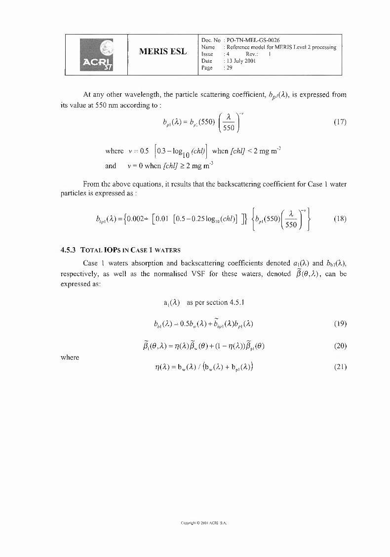
At any other wavelength, the particle scattering coefficient, bp1(A), is expressed fromits value at 550 nm according to :
(;., )-v
bp1(A)=b"1(550) -550
(17)
where v = 0.5 r0.3 - logl 0 (chi)1 when [chi} < 2 mg m"3
and v = 0 when [chi} ~ 2 mg m-3
From the above equations, it results that the backscattering coefficient for Case 1waterparticles is expressed as :
b,,,(A)= {0.002+ [0.0I [0.5-0.25 log,,(chl)] ]} {b,,(ssoi( S~Or} (18)
4.5.3 TOTAL IOPS IN CASE 1 WATERS
Case 1 waters absorption and backscattering coefficients denoted a1(A) and bb1(A),respectively, as well as the normalised VSF for these waters, denoted /3(8,A), can beexpressed as:
a1(A) as per section 4.5.1
(19)
where
- - -/3,(8,A) = 7J(A)/3w(8) + (l - 71(A))/3p1(8)
7J(A) = bw(A) I (bw(A) + bp,(A))
(20)
(21)
Copyright© 2001ACRI S.A.

MERIS ESLDoc. No : PO-TN-MEL-GS-0026Name : Reference model for MERIS Level 2 processingIssue : 4 Rev.: IDate : 13 July 200 IPage : 30
4.5.4 WARNING CONCERNING THE USE OF THE MODEL FOR CASE 1 WATERS IOPs: STATEOF-THE-ART AND UNCERTAINTIES
4.5.4.1 Raman EmissionThe Raman emission by water molecules is a trans-spectral (or inelastic) scattering
process by which absorbed energy at a given wavelength .A.' is re-emitted as radiation at longerwavelengths around A. The Raman VSF f3R(8) is symmetrical with respect to e = rr/2 andexpresses as :
(5)
f3R(8) = 0.067 (1+0.55 cos2(8)) (4)
The Raman emission undergoes a frequency shift that is independent of the incident frequencyand thus occurs within the whole (visible) spectrum. According to Walrafen (1967), the shapeof the redistribution function fR(KR) is the sum of 4 Gaussian functions (i = 1 to 4) :
where K'Ris the wavenumber shift of the Raman emission, Ki is the centre of the ithGaussianfunction, LlK'i the width at half maximum of this function and the A/s are the weights of eachfunction (see table 4.5.4-1).
1 A x; (em+) Llx:i (cm+)I
1 0.41 3250 2102 0.39 3425 1753 0.10 3530 1404 0.10 3625 140
Table 4.5.4-1: Data from Walrafen (1967)
To an incident (exciting) radiation with a wavelength /l' and a wavenumber K" willcorrespond a Raman emission within a spectral band described by Eq. (5) such as K'= K" - #,leading to redistribution functions expressed in terms of wavelengths fR(A.'~ /\.)as shown inFig. 4.3 below.
The magnitude of the phenomenon is expressed through the Raman coefficient aR(A.!)through
ee
aR(A') = JbR(A' -7 A) dAA.'
(6)
where bR is the Raman scattering coefficient for an exciting wavelength A' and an emission atwavelength A (A> A'). This coefficient, according to recent determinations at 488 nm, is:
Copyright 10200 I ACRI S.A.

MERIS ESL
it varies according to a k5 law.
Doc. No : PO-TN-MEL-GS-0026Name : Reference model for MERIS Level 2 processingIssue : 4 Rev.: 1Date : 13 July 2001Page : 31
aR(488) = 2.6 l0-4 rrr! (7)
This phenomenon is important in clear Case I waters (low Chi) to the extent that theelastic scattering is low, in the red part of the spectrum in particular. With an almost isotropicfunction (Eq. (4)), it strongly modifies the upward radiance distribution and thus affects the Q(and f/Q) behaviour.
0.20
c- 0.15I
Ec-.......0.10-<t::.:.•....•"'~ 0.05
),' • 450 nm
),' •• 500 ""'A'"' !50-
0.00 I . ' . I I 1 •• I I •• I 6 I •• • I ••• •Jo.
400 450 500 550 600wavelength >. (nm)
650 700
Figure 4.3. : the Raman wavelength redistribution function jR(A' ~ /...),for selected incidentwavelengths A.'. Figure reproduced from Mobley (1994).
Conversely the Raman emission at a fixed wavelength A is excited by a spectral band centredon A', the shape of which is approximately the reverse image of those shown in thisfigure.
4.5.4.2 Fluorescence by Phytoplankton
The emission of fluorescence by phytoplankton is isotropic ( ~F (8) = constant). Itsintensity depends on the chlorophyll-a concentration and on the quantum yield forfluorescence, </>r- This yield </>r is defined as the number of photons emitted divided by thenumber of photons absorbed by the algal cells. It is known as being varying within a factor of10, approximately with the lower values observed near the surface (Maritorena et al. 2000). If</>r is fixed, this emission can be (but has not been) incorporated into the IOP model for Case 1waters. Any radiation within the 380-680 nm domain, after being weighted by the algalabsorption spectrum, is able to excite the Chi-a fluorescence around 683 nm. In contrast, theemission spectrum is independent from the excitation spectrum and is currently modelled(e.g., see Gordon, 1979; Kattawar and Valerio, 1982; Kishino et al., 1984; Sathyendranath andPlatt, 1998) as a Gaussian spectral distribution, peaked around 683 nm, and with a standarddeviation CJ= 10.64 nm, corresponding to a width of about 25 nm at half maximum (see Fig.4.4). This curve, modelled through exp(-(A.- 683) I 2cr2) accounts very well for observationsfor natural populations as well as for algae grown in culture, except beyond 710 nm where aweak shoulder (around 730 nm) often appears.
Copyright ID2001 ACRI SA

Doc. No : PO-TN-MEL-GS-0026Name : Reference model for MERIS Level 2 processingIssue : 4 Rev.: 1Date : 13 July 2001Page : 32
MERIS ESL
683 nm
100 - v~~
-
I'"' -
- I \ -125.1nmJ
- I \ -
l35.4nmlI I ..
t- I \ -
145.7nm Ir.v ·~-- I--
80
60
40
20
0660 670 680 690 700 710
Figure 4.4. : Typical Gaussian spectral distribution for the Chi-afluorescence, peakedaround 683 nm, and with a standard deviation o = 10.64 nm, corresponding to a width of
about 25 nm at half maximum
4.5.4.3 Fluorescence by Endogenous YellowSubstanceThis term which may be important in presence of high amount of yellow substance is
less documented than the chlorophyll-a fluorescence, and depends on the chemicalcomposition of the organic matter collectively forming the "yellow substance". This emissionis believed to be negligible in Case 1 waters, and has not been incorporated within the IOPmodel for Case 1waters.
4.5.4.4 Other Warnings and LimitationsThe Case 1 waters IOP model include some uncertainties in its parameterisation or
even some assumptions. These properties with their corresponding uncertainties are listed intable 4.5.4-2 below. The column "Expectation" indicates which scientific evolutions areforeseen.
Copyrightc 200I ACRI S.A.

MERIS ESLDoc. No : PO-TN-MEL-GS-0026Name : Reference model for MERIS Level 2 processingIssue : 4 Rev.: IDate : 13 July 2001Page : 33
IOP Equation number Comment Expectationor table
aw(A) Table 4.4.1-1 Known with sufficient accuracy Will not evolveaR().) Eqs. (6) and (7), Known with sufficient accuracy Will not evolve
Table 4.5 .4-1ai (A.) Eqs. (8) to (11"), Well documented for World Ocean (but see Will not evolve
Table 4.5.1-1 and the large variation factor). Seasonal significantly4.5.1-2 variability under investigation.
s.o: Eqs. (3) and (3 ') Known with sufficient accuracy Will not evolvebp1(A.) Eqs. (16) and (17) Well documented for World Ocean (but see Will not evolve
the large variation factor) significantlybbp1(A.) Eqs. (15) and (18) Best guess Could evolve
~w(8,A.) Eqs. (2) and (2') Slight uncertainty on p; very weak influence Will not evolveon the result
fY(e) Eqs. (4) and (5) Known with sufficient accuracy Will not evolve
~p(8) Eqs. (12) to (14), Could evolveTable 4.5.2-1 andTable 4.5.2-2
Table 4.5.4-2: Comments on model parameterisation
As a general warning, the present model is based on statistical relationships (betweenKd or bp and Chl) that represent "average" situations. Therefore, its use as a predictive toolleads to various results when the large standard errors associated with each input parametersare taken into account; it may fail when compared case by case to actual data (as reflectancefor instance).
Copyright © 200 I ACRI SA
II Doc. No : PO-TN-MEL-GS-0026
MERIS ESL Name : Reference model for MERIS Level 2 processingIssue : 4 Rev.: I- •
Date : 13 July 2001Page : 34
4.6 CASE 2 WATERS IOPS
4.6.1 INTRODUCTION
Water constituents comprise a large number of different substances, which includemineralic dissolved and particulate compounds, a large variety of organic macromolecules,living organisms such as phytoplankton, zooplankton, bacteria etc. and their debris andexcrements. All of these constituents of water exhibit different optically properties concerningscattering and absorption.
For the purpose of optical remote sensing this diversity of substances has to begrouped into a small number of classes each of which includes constituents with similaroptical properties and I or correlated concentrations. For the majority of the world ocean areasit is sufficient to comprise all substances into one group using phytoplankton chlorophyll a asa proxy. This type of water is called case I water. The concentration of this class of substances- in terms of chlorophyll a - can be derived from the blue to green shift of the water colour. Inmany coastal waters one needs more than one class of substances to describe the variability ofwater colour. By tradition and experience three classes are defined: (1) phytoplankton pigmentwith chlorophyll a as a proxy, (2) the dry weight of all particles (total suspended matter, TSM)and (3) the absorption caused by the dissolved fraction of all water constituents (gelbstoff).Dissolved and particulate is defined by the pore size of the filter used for separation, whichtraditionally was 0.45 µm and nowadays is 0.2 µm.
However, each of the three groups of substances is variable with respect to theircomposition and thus their chemical, physical and in particular optical properties. Any remotesensing system and retrieval algorithm has to take this variability into account.
For the MERIS case 2 water algorithm two approaches have been prepared. Oneapproach, endorsed in the previous issue of this document, is to base the algorithm directly onoptical and concentration measurements and harmonize the case 2 with the case 1 algorithm.The other approach, which is described here, uses optical components, which do not directlyreflect a water constituent, but which describe the dominant optical property of a group ofsubstances. The quantitative relationship between the concentration of a bio-geochemicalcomponent and its optical proxy is described by a conversion factor or equation, which can beadapted by the user based on his experience to local conditions.
This alternative model is based on the experience with the first MERIS referencemodel (Version of 1996) as well as on measurements of water constituents (concentrations,scattering and absorption) during the marine optics projects COASTIOOC, COLORS andMAPP.
Due to the restrictions of the MERIS processor, only three components can be defined.For this model these are:
(1) phytoplankton pigment absorption ap;g,(2) absorption of all other substances ayp(dissolved gelbstoff ay and bleached particulate
matter ap) and
Copyright© 2001ACRI S.A.
MERIS ESLDoc. No : PO-TN-MEL-GS-0026Name : Reference model for MERIS Level 2 processingIssue : 4 Rev.: IDate : 13 July 2001Page : 35
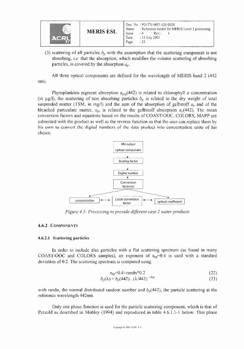
(3) scattering of all particles bp with the assumption that the scattering component is notabsorbing, i.e. that the absorption, which modifies the volume scattering of absorbingparticles, is covered by the absorption ap.
All three optical components are defined for the wavelength of MERIS band 2 (442nm).
Phytoplankton pigment absorption ap;g(442) is related to chlorophyll a concentration(in µg/l), the scattering of non absorbing particles bp is related to the dry weight of totalsuspended matter (TSM, in mg/I) and the sum of the absorption of gelbstoff ay and of thebleached particulate matter, aP, is related to the gelbstoff absorption ay( 442). The meanconversion factors and equations based on the results of COASTIOOC, COLORS, MAPP aresubmitted with the product as well as the reverse function so that the user can replace them byhis own to convert the digital numbers of the data product into concentration units of hischoice.
NN output
optical component
Scaling factor
Digital number
+
concentration Local conversionfactor
Figure 4.5: Processing to provide different case 2 water products
4.6.2 COMPONENTS
4.6.2.1 Scattering particles
In order to include also particles with a flat scattering spectrum (as found in manyCOASTIOOC and COLORS samples), an exponent of Sbp=0.4 is used with a standarddeviation of 0.2. The scattering spectrum is computed using
Sbp=O.4+randn *0.2bp('A)= bp(442). (A./442)-sbp
(22)(23)
with randn, the normal distributed random number and bp(442), the particle scattering at thereference wavelength 442nm.
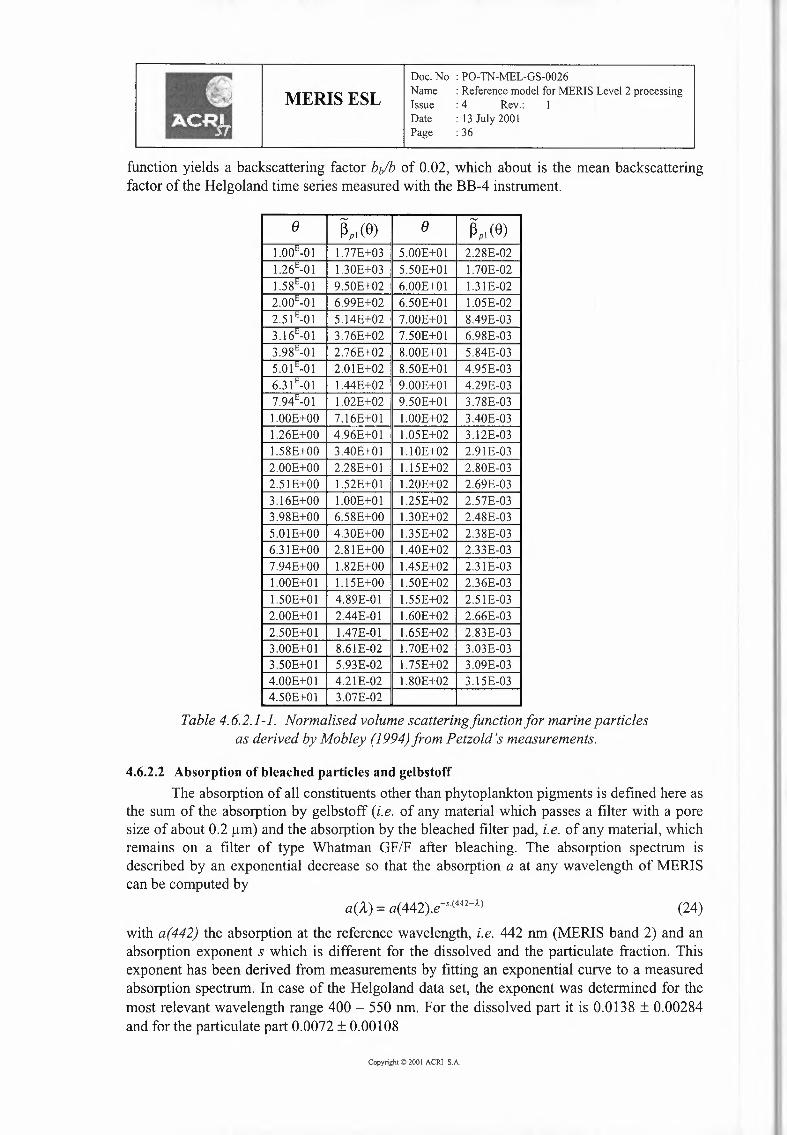
Only one phase function is used for the particle scattering component, which is that ofPetzold as described in Mobley (1994) and reproduced in table 4.6.1.1-1 below. This phase
Copyright © 200 I ACRI S.A
II)- MERIS ESLDoc. No : PO-TN-MEL-GS-0026Name : Reference model for MERIS Level 2 processingIssue : 4 Rev.: 1Date : 13 July 2001Page : 36
function yields a backscattering factor bi/b of 0.02, which about is the mean backscatteringfactor of the Helgoland time series measured with the BB-4 instrument.
()~pl (8) ()
~pl (8)1.00E-01 l.77E+03 5.00E+Ol 2.28E-021.26E-01 l.30E+03 5.50E+Ol 1.70E-021.58E-01 9.50E+02 6.00E+Ol 1.3lE-022.ooE-01 6.99E+02 6.50E+Ol 1.05E-022.51E-01 5.14E+02 7.00E+Ol 8.49E-033.16E-01 3.76E+02 7.50E+Ol 6.98E-033.98E-01 2.76E+02 8.00E+Ol 5.84E-035.01E-01 2.0IE+02 8.50E+Ol 4.95E-036J1E-01 l .44E+02 9.00E+Ol 4.29E-037.94E-01 1.02E+02 9.50E+Ol 3.78E-031.00E+OO 7.16E+Ol 1.00E+02 3.40E-031.26E+OO 4.96E+Ol 1.05E+02 3.12E-031.58E+OO 3.40E+Ol 1.10E+02 2.91E-032.00E+OO 2.28E+Ol 1.15E+02 2.80E-032.51E+OO 1.52E+Ol 1.20E+02 2.69E-033.16E+OO 1.00E+Ol 1.25E+02 2.57E-033.98E+OO 6.58E+OO 1.30E+02 2.48E-035.0IE+OO 4.30E+OO 1.35E+02 2.38E-036.31E+OO 2.81E+OO 1.40E+02 2.33E-037.94E+OO 1.82E+OO 1.45E+02 2.3 lE-03l.OOE+Ol l.15E+OO 1.50E+02 2.36E-031.50E+Ol 4.89E-01 1.55E+02 2.51E-032.00E+Ol 2.44E-01 1.60E+02 2.66E-032.50E+Ol 1.47E-01 1.65E+02 2.83E-033.00E+Ol 8.61E-02 l.70E+02 3.03E-033.50E+Ol 5.93E-02 l .75E+02 3.09E-034.00E+Ol 4.21E-02 l.80E+02 3.15E-034.50E+Ol 3.07E-02
Table 4.6.2.1-1. Normalised volume scattering function for marine particlesas derived by Mobley (1994)from Petzold 's measurements.
4.6.2.2 Absorption of bleached particles and gelbstoffThe absorption of all constituents other than phytoplankton pigments is defined here as
the sum of the absorption by gelbstoff (i.e. of any material which passes a filter with a poresize of about 0.2 µm) and the absorption by the bleached filter pad, i.e. of any material, whichremains on a filter of type Whatman GF/F after bleaching. The absorption spectrum isdescribed by an exponential decrease so that the absorption a at any wavelength of MERIScan be computed by
a(ll.)= a(442).e-s.(442-A.) (24)with a(442) the absorption at the reference wavelength, i.e. 442 nm (MERIS band 2) and anabsorption exponent s which is different for the dissolved and the particulate fraction. Thisexponent has been derived from measurements by fitting an exponential curve to a measuredabsorption spectrum. In case of the Helgoland data set, the exponent was determined for themost relevant wavelength range 400 - 550 nm. For the dissolved part it is 0.0138 ± 0.00284and for the particulate part 0.0072 ± 0.00108
Copyright© 2001ACRI S.A.
MERIS ESLDoc. No : PO-TN-MEL-GS-0026Name : Reference model for MERIS Level 2 processingIssue : 4 Rev.: 1Date : 13 July 2001Page : 37
COASTIOOC values have been derived from the wavelength range 350-500, this givesa higher mean exponent of 0.0176 ± 0.002. When using this wavelength range we got a meanexponent of 0.0154 ± 0.0019 from the Helgoland series.
The mean exponent of particle absorption of the COASTIOOC data set is 0.0123 witha standard deviation of 0.00126, again derived from the wavelength range 350 - 500 nm.
Since the dissolved and particulate absorption fraction has to be combined to one, i.e.the absorption of all water constituents except phytoplankton pigments, a.; we use thecovariance between the dissolved and particulate absorption from the Helgoland data set, asexpressed in the following relationships with randu, the random number from a uniformdistribution between 0 and 1:
ayct(442) = [ 0.005 ... 1.5]ayct(442)=exp(ln(0.005)+randu*(ln (1.5)- ln (0.005)))
ayp(442)=2*rand*ayct(442)
(25)(26)(27)
The spectral exponent was computed as:
Syct= 0.014 + randn*0.003Syp= 0.007 + randn*0.001
ayct(A)= ayct(442)* exp(-Syct*(A- 442))ayp(A)= ayp(442)* exp(-syp*(A. - 442))
(28)(29)(30)(31)
4.6.2.3 Pigment AbsorptionThe pigment absorption component is determined from measurements of filter pad
absorption. It is the absorption of the bleachable fraction of the material, which does not passthe filter, i.e. the difference between the absorption of the filter pad before and after bleaching.
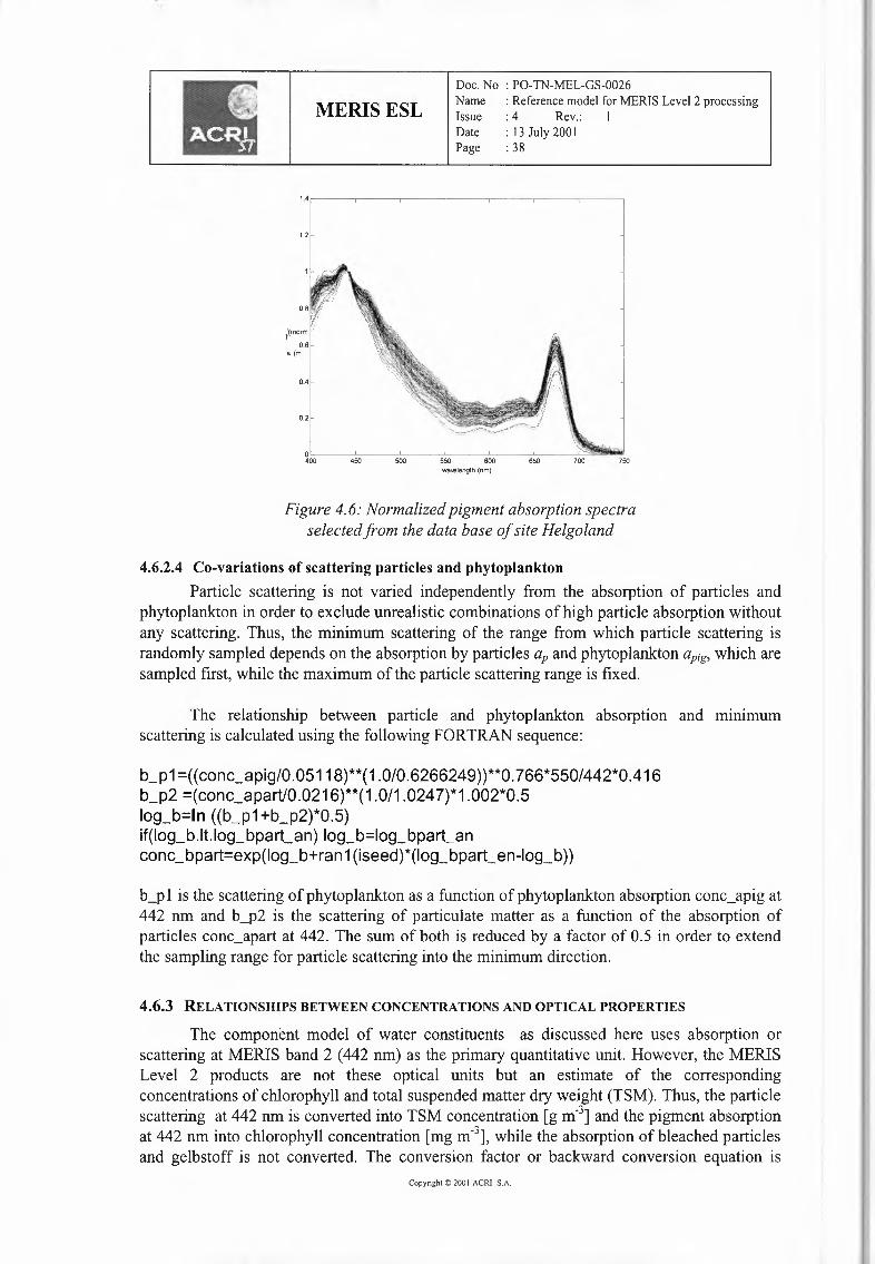
The time series of Helgoland shows two different types of spectra with all transitions,a typical summer spectrum with a clear maximum around 440 nm and a winter spectrumwithout a clear maximum but with a nearly exponential decrease in the blue-green spectralrange. Since it is assumed that the winter spectra are dominated by detritus which containdegradation products of chlorophyll only the summer spectrum have been used for thecomponent model. In order to include the variance of these summer spectra, a set of 77 spectrahaven been selected with a clear absorption peak at 442 nm. One of these spectra is selectedrandomly for the computation of the reflectances. The 77 spectra were selected afternormalisation by apig(442) according to the following criteria:
apign(442)I apign(412)> 0.98apign(442)I apign(448)> 1.0
(32)(33)
Copynght !) 200I ACRI S.A.
MERIS ESLDoc. No : PO-TN-MEL-GS-0026Name : Reference model for MERIS Level 2 processingIssue : 4 Rev.: IDate : 13 July 2001Page : 38
1.4 -.------ -----------,-----------,-------~---~---
0.4
12~
!o~'---~---~-400 450 500 550 600 650 700 750
1))norm0.6
a (m
0.2
wa-.elength (nm)
Figure 4.6: Normalized pigment absorption spectraselected from the data base of site Helga/and
4.6.2.4 Co-variations of scattering particles and phytoplanktonParticle scattering is not varied independently from the absorption of particles and
phytoplankton in order to exclude unrealistic combinations of high particle absorption withoutany scattering. Thus, the minimum scattering of the range from which particle scattering israndomly sampled depends on the absorption by particles ap and phytoplankton apig, which aresampled first, while the maximum of the particle scattering range is fixed.
The relationship between particle and phytoplankton absorption and mimmumscattering is calculated using the following FORTRAN sequence:
b_p1=((conc_apig/0.05118)**( 1.0/0.6266249) )**O.766*550/442*0.416b_p2 =(conc_apart/0.0216)**(1.0/1.0247)*1.002*0.5log_b=ln ((b_p1+b_p2)*0.5)if(log_b.lt.log_bpart_an) log_b=log_bpart_anconc_bpart=exp(log_b+ran 1(iseed)* (log_bpart_ en-log_b))
b_pl is the scattering of phytoplankton as a function of phytoplankton absorption conc_apig at442 nm and b_p2 is the scattering of particulate matter as a function of the absorption ofparticles conc_apart at 442. The sum of both is reduced by a factor of 0.5 in order to extendthe sampling range for particle scattering into the minimum direction.
4.6.3 RELATIONSHIPS BETWEEN CONCENTRATIONS AND OPTICAL PROPERTIES
The component model of water constituents as discussed here uses absorption orscattering at MERIS band 2 (442 nm) as the primary quantitative unit. However, the MERISLevel 2 products are not these optical units but an estimate of the correspondingconcentrations of chlorophyll and total suspended matter dry weight (TSM). Thus, the particlescattering at 442 nm is converted into TSM concentration [g m-3] and the pigment absorptionat 442 nm into chlorophyll concentration [mg m"], while the absorption of bleached particlesand gelbstoff is not converted. The conversion factor or backward conversion equation is
Copyright© 200I ACRI S.A.

MERIS ESLDoc. No : PO-TN-MEL-GS-0026Name : Reference model for MERIS Level 2 processingIssue : 4 Rev.: 1Date : 13 July 2001Page : 39
published in order to enable users to compute the initial optical units and then apply their ownconversion algorithms, which might be better adapted to their area under research.
4.6.3.1 Relationship between particle scattering and TSM dry weightAccording to the COASTIOOC results,
bp(555) = Abp(555) * <TSM> (g m")with Abp=0.5 m2 g-1 and a factor of variation of 1.2.
(34)
The absorption of these particles after bleaching isap(443)= Aap*<TSM> Bap
with Aap=0.0216 and Bap=l.0247 and a factor of variation of Aapof 1.84(35)
Since the single scattering albedo near the IR region is close to 1, the value of 0.93 forA around 780 nm is used to modify the conversion factor of 0.5 for non absorbing particles.Because of the assumed spectral scattering exponent of 0.4, the conversion factor is estimatedaccording to the following scheme:
hp(442)=bp(780)*(442/780)-0.4 (36)
the conversion factor for non absorbing particles is then
Abp(442) = (442/780) -0.4* 0.92*0.5 = 0.577bp(442) = Abp(442) * <TSM> (g m")
(37)(38)
and the reverse relationship
<TSM> (g m") = 1.73 * bp(442) (39)
4.6.3.2 Relationship between pigment absorption and chlorophyll a concentrationThe relationship between chlorophyll a concentration and the difference of the
absorption at 442 nm of the filterpad before and after bleaching was determined for the 77selected spectra as:
In (chl)= 3.2662+0.77135*ln (apil442 nm))chl = 26.212* <apig(442)> ·77135
(40)(41)
with a correlation coefficient ofr = 0.69475
The inverse relationship isapig(442)= 0.041457*<chl>o.62576 (42)
Copyrighte 2001ACRI S.A
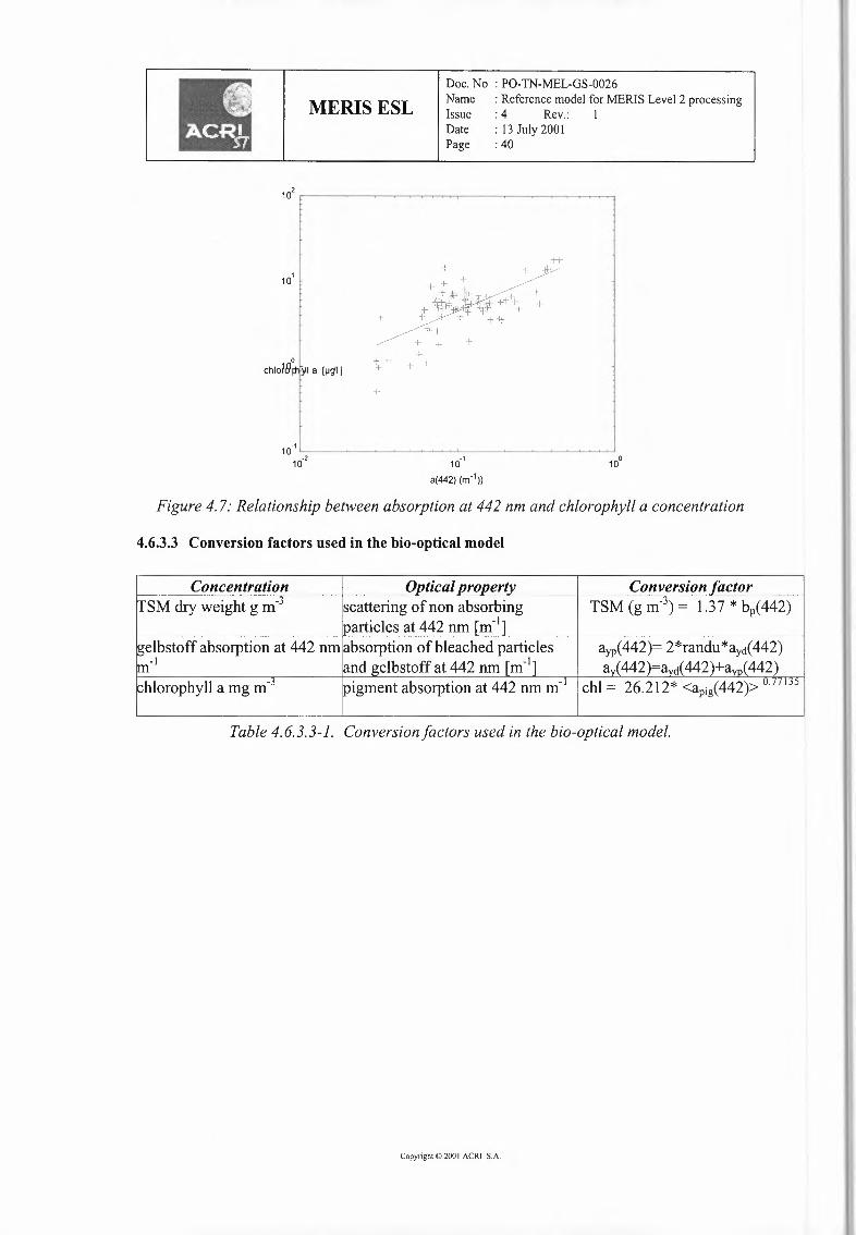
Conversion factor
MERIS ESLDoc. No : PO-TN-MEL-GS-0026Name : Reference model for MERIS Level 2 processingIssue : 4 Rev.: 1Date : 13 July 200 IPage : 40
o I .L +chloli9ot~Ia [µg'I) +
J
10-~1-- -----~--·--·~ ~~ --~ J10·1 ~- _,_ ~-~
a(442) (m-1)) 10°
Figure 4.7: Relationship between absorption at 442 nm and chlorophyll a concentration
4.6.3.3 Conversion factors used in the bio-optlcal model
ConcentrationTSM (g m")> 1.37 * bp(442)SM dry weight g m"
igment absorption at 442 nm m-1
elbstoff absorption at 442 nm-I
bsorption of bleached particlesnd zelbstoff at 442 nm rm"
hlorophyll a mg m'
Table 4.6.3.3-1. Conversionfactors used in the bio-optical model.
Copyright© 2001ACRI SA
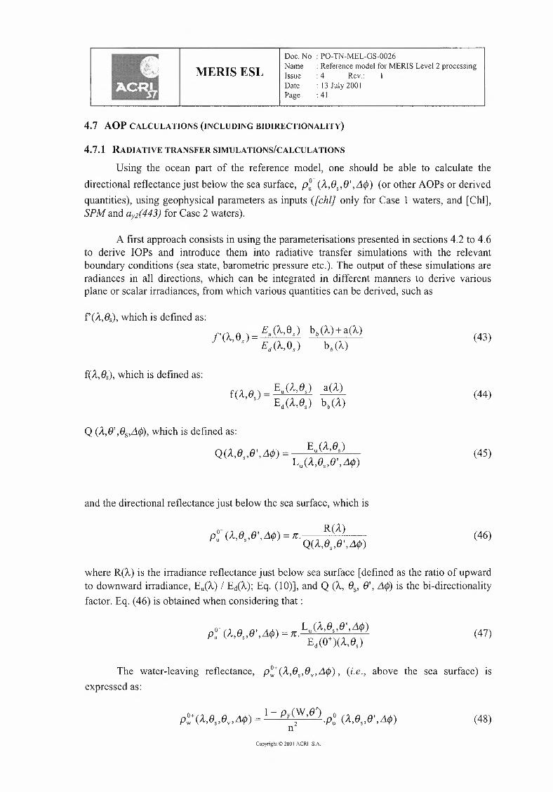
MERIS ESLDoc. No : PO-TN-MEL-GS-0026Name : Reference model for MERIS Level 2 processingIssue : 4 Rev.: 1Date : 13 July 2001Page : 41
4.7 AOP CALCULATIONS (INCLUDING BIDIRECTIONALITY)
4. 7.1 RADIATIVE TRANSFER SIMULATIONS/CALCULATIONS
Using the ocean part of the reference model, one should be able to calculate thedirectional reflectance just below the sea surface, p~- (ll,e,,e',L1<f>) (or other AOPs or derivedquantities), using geophysical parameters as inputs ([ch!] only for Case 1 waters, and [Chi],SPM and ay2(443) for Case 2 waters).
A first approach consists in using the parameterisations presented in sections 4.2 to 4.6to derive IOPs and introduce them into radiative transfer simulations with the relevantboundary conditions (sea state, barometric pressure etc.). The output of these simulations areradiances in all directions, which can be integrated in different manners to derive variousplane or scalar irradiances, from which various quantities can be derived, such as
f'(A.,88), which is defined as:
(43)
f(ll,8s), which is defined as:
(44)
Q (A.,8' ,es,Ll<f>),which is defined as:
Q( lle 8' L1"')= Eu(/l,8,)' '' ' 'I' L (/le 8' L1"')
u ' s' ' o/(45)
and the directional reflectance just below the sea surface, which is
R(/l)P~- (A.,e,,e',L1<f>) = ti.Q(A.,e,,e',L1<f>) (46)
where R(A) is the irradiance reflectance just below sea surface [defined as the ratio of upwardto downward irradiance, Eu(A) I Ect(A);Eq. (1O)], and Q (A.,es, 8', L1<f>)is the bi-directionalityfactor. Eq. (46) is obtained when considering that :
(47)
The water-leaving reflectance, p~+(A.,e,,ev,L1<f>), (i.e., above the sea surface) isexpressed as:
0+(18 8 ) 1-pF(W,8') o-(,8 8' )Pw /\,,' s > v,L1<{> = ? ·Pu /\,,' s' ,L1<{>n
(48)
Copyright© 200I ACRI S.A.
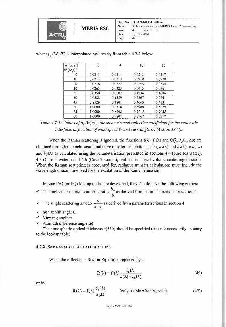
II..- MERIS ESLDoc. No : PO-TN-MEL-GS-0026Name : Reference model for MERIS Level 2 processingIssue : 4 Rev.: 1Date : 13 July 2001Page : 42
where p[i{_W, 8') is interpolated by-linearly from table 4.7-1 below.
W (m.s') 0 4 10 160' (deg)\
0 0.0211 0.0211 0.0213 0.021710 0.0211 0.0213 0.0218 0.022820 0.0218 0.0227 0.0255 0.033430 0.0265 0.0325 0.0613 0.096135 0.0350 0.0602 0.1234 0.168640 0.0588 0.1559 0.2367 0.274145 0.1529 0.3801 0.4065 0.413150 1.0000 0.6718 0.5988 0.562955 1.0000 0.8905 0.7715 0.705560 1.0000 0.9807 0.8967 0.8277
(49)
Table 4.7-1: Values of pp(W, 8 '),the mean Fresnel reflection coefficient for the water-airinterface, asfunction of wind speed Wand view angle 8', (Austin, 1974).
When the Raman scattering is ignored, the functions f(.11.),f(A.) and Q(A.,88,Sv,~<1>)areobtained through monochromatic radiative transfer calculations using a1(A.) and b 1(A.) or aAA.)and bAA.) as calculated using the parameterisation presented in sections 4.4 (pure sea water),4.5 (Case 1 waters) and 4.6 (Case 2 waters), and a normalised volume scattering function.When the Raman scattering is accounted for, radiative transfer calculations must include thewavelength domain involved for the excitation of the Raman emission.
In case f' IQ (or f/Q) lookup tables are developed, they should have the following entries:
./ The molecular to total scattering ratio bw as derived from parameterisations in section 4.b
./ The single scattering albedo _b_ as derived from parameterisations in section 4a+b
./ Sun zenith angle Ss
./ Viewing angle 8'
./ Azimuth difference angle ~<1>The atmospheric optical thickness 1(550) should be specified (it is not necessarily an entry
to the lookup table).
4.7 .2 SEMI-ANALYTICAL CALCULATIONS
When the reflectance R(A) in Eq. (46) is replaced by:
or by
R(A.)= f(A.)bb(A.)a(A.)
(only usable when bb << a) (49')
Copyright© 200I ACRI S.A.

MERIS ESLDoc. No : PO-TN-MEL-GS-0026Name : Reference model for MERIS Level 2 processingIssue : 4 Rev.: IDate : 13 July 200 IPage : 43
Then p~+(A,85,8v,L1¢)can be expressed as:
f(A,85) [bb(A)]P~+(A,8s,8',L1</>) = rr 9\(8') Q(A.,8s,8',L1</>) a(A) (50)
which is also obtained by combining the following basic equations (see also the table ofsymbols in section 2.5):
L = L i- PFw u ----n2
The semi-analytical Eq. (50) can be used along with the parameterisations developedin section 4.2 to 4.6.1. In that case, a(A.) and bb(A)can be broken into individual contributionsby the different water constituents, following the "analytical approach" (but see introductionto section 4.5.1).
N
a(A.) = Lan(A.)n=1
(51)
N -bb(A)= Lbbn(A)bn(A)
n=1
(52)
where the subscript n indicates a given optically significant seawater constituent, bn(A) is thescattering coefficient of the n1h substance and bbn(A.) is the ratio of backscattering toscattering (or backscattering efficiency) of the n1h substance.
In Eq. (50) above, the "gothic" 9\ factor (Morel and Gentili, 1996) is interpolated fromtable 4.7-2 below.
W (m.s')0 4 8 168' (deg)\
0 0.528883 0.528867 0.528824 0.5285811 0.528899 0.528856 0.528797 0.5285972 0.528894 0.528883 0.528775 0.5286133 0.528878 0.52884 0.528829 0.5286134 0.528867 0.528883 0.528845 0.5285925 0.528872 0.528905 0.528824 0.5285976 0.528878 0.528851 0.528829 0.5285597 0.528856 0.528856 0.528824 0.5284028 0.528851 0.528867 0.528862 0.5283599 0.528856 0.528878 0.52877 0.52827810 0.528856 0.528883 0.528764 0.52808911 0.528899 0.528905 0.528673 0.52773812 0.528889 0.528802 0.528608 0.527625
Copyright© 200I ACRI SA

MERIS ESLDoc.No : PO-TN-MEL-GS-0026Name : Referencemodel for MERISLevel 2 processingIssue : 4 Rev.: IDate : 13July 2001Page : 44
W (m.s")0 4 8 16e· (deg)\
13 0.528883 0.528775 0.528532 0.52739214 0.528851 0.5287 0.528489 0.5268915 0.528813 0.528608 0.528316 0.52644716 0.528732 0.528554 0.528089 0.52594517 0.528727 0.528446 0.528008 0.52504818 0.528646 0.528381 0.527846 0.5238719 0.528613 0.5283 0.5275 0.52286520 0.528548 0.528084 0.527279 0.5219821 0.528467 0.5279 0.526998 0.52019222 0.528365 0.527679 0.526144 0.51817723 0.52824 0.527371 0.525448 0.51596224 0.528014 0.526976 0.524616 0.5131825 0.527851 0.526831 0.523416 0.51057626 0.527614 0.526053 0.522061 0.50700527 0.52736 0.525593 0.52051 0.50311128 0.526982 0.524902 0.51842 0.49877329 0.526474 0.523508 0.515708 0.49339230 0.52602 0.521947 0.511937 0.48740231 0.525307 0.520035 0.50794 0.4813332 0.524545 0.517836 0.503089 0.47447533 0.5236 0.514968 0.497228 0.4664834 0.522309 0.510771 0.490238 0.4580235 0.520899 0.505082 0.482119 0.44875636 0.51909 0.498659 0.472968 0.43851437 0.516891 0.490292 0.461931 0.42847238 0.513801 0.47965 0.44975 0.41704739 0.510274 0.46742 0.436121 0.40448240 0.505412 0.451889 0.421482 0.39184141 0.499173 0.434063 0.405481 0.37847142 0.48872 0.413638 0.387114 0.36326543 0.474221 0.390988 0.368575 0.34836644 0.449583 0.365242 0.346011 0.33338145 0.412601 0.336671 0.324193 0.31779746 0.359554 0.306188 0.302239 0.30286647 0.287908 0.275208 0.280156 0.28776748 0.209752 0.243574 0.256517 0.27001149 0.136037 0.21375 0.234029 0.25409750 0.0755841 0.184504 0.21093 0.23746451 0.0361985 0.154728 0.189511 0.22188552 0.0140559 0.128167 0.168395 0.2064953 0.00447281 0.103831 0.146798 0.1911854 0.0011182 0.0826552 0.127189 0.17570955 0.000226882 0.0627274 0.108666 0.16133556 0 0.0460786 0.0914604 0.14522157 0 0.0326278 0.0748656 0.13052758 0 0.0220994 0.0596105 0.11600759 0 0.0141207 0.0463325 0.101784
Copyright© 200I ACRI S.A.
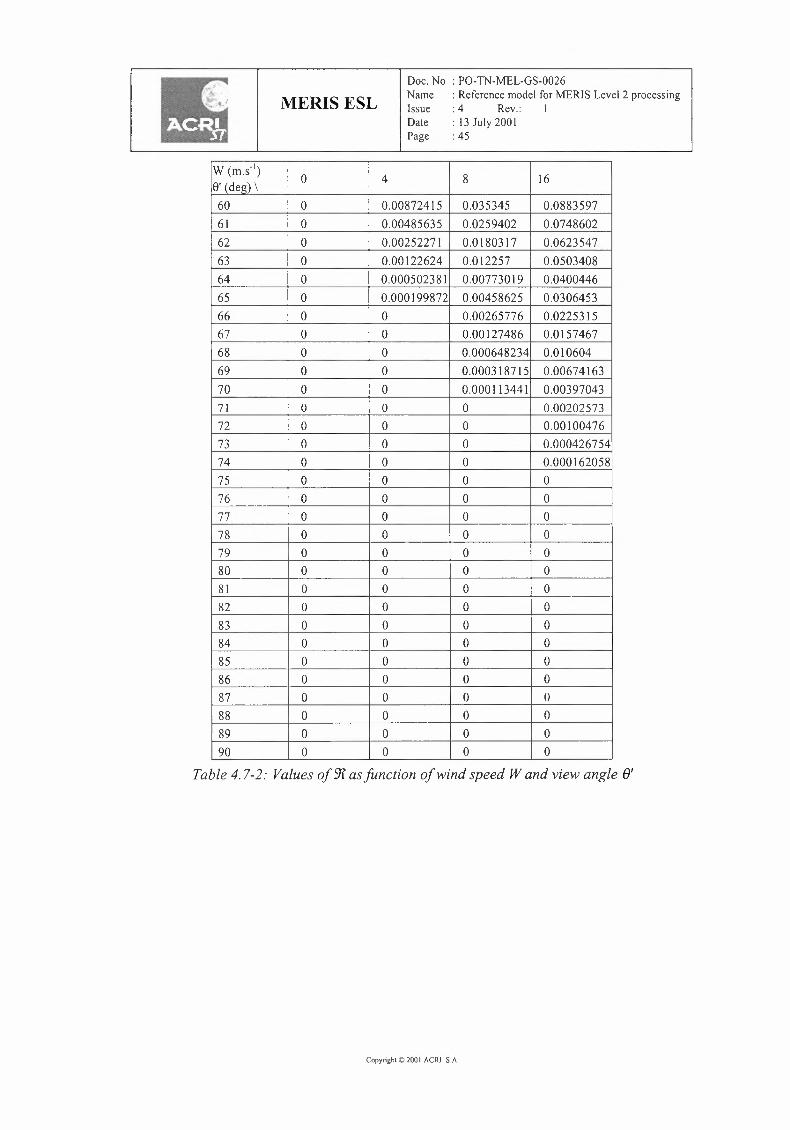
MERIS ESLDoc. No : PO-TN-MEL-GS-0026Name : Reference model for MERIS Level 2 processingIssue : 4 Rev.: 1Date : 13 July 2001Page : 45
W (m.s')0 4 8 16e· (deg)\
60 0 0.00872415 0.035345 0.088359761 0 0.00485635 0.0259402 0.074860262 0 0.00252271 0.0180317 0.062354763 0 0.00122624 0.012257 0.050340864 0 0.0005023 81 0.00773019 0.040044665 0 0.000199872 0.00458625 0.030645366 0 0 0.00265776 0.022531567 0 0 0.00127486 0.015746768 0 0 0.000648234 0.01060469 0 0 0.000318715 0.0067416370 0 0 0.000113441 0.0039704371 0 0 0 0.0020257372 0 0 0 0.0010047673 0 0 0 0.00042675474 0 0 0 0.00016205875 0 0 0 076 0 0 0 077 0 0 0 078 0 0 0 079 0 0 0 080 0 0 0 081 0 0 0 082 0 0 0 083 0 0 0 084 0 0 0 085 0 0 0 086 0 0 0 087 0 0 0 088 0 0 0 089 0 0 0 090 0 0 0 0
Table 4.7-2: Values of 91asfunction of wind speed Wand view angle B'
Copynght 10200 I ACRI S.A.
MERIS ESLDoc. No : PO-TN-MEL-GS-0026Name : Reference model for MERIS Level 2 processingIssue : 4 Rev.: 1Date : 13 July 200 IPage : 46
5. Sea surface state
5.1 SPECULAR REFLECTION
The effect of the air-sea interface shape on Fresnel reflection and refraction will beaccounted for by applying statistics of Cox and Munk (1954), assuming an isotropicdistribution of waves and a variable wind speed.
If a code like FUB's MOMO is used to calculate TOA radiances (reflectances), thenthe glint reflectance at the TOA level has to be calculated independently (see below), andsubtracted from the total signal calculated by the code at the TOA (for any combination of es,8y, and .1¢). In its actual state, this code does not provide information on the history ofphotons and cannot therefore separate the contributions from the sea surface from the totalTOA signal. When generating the LUTs with the coefficients of the quadratic equation linking[Ppath I Pr] to Ta) for atmospheric correction of MERIS data, this subtraction must beperformed on the reflectances for the pure Rayleigh atmospheres CPr) as well as for therealistic atmospheres (molecules + aerosols, Ppath), before the corresponding reflectances areratioed and related to the aerosol optical thickness.
As far as a standard version of the MOMO code is used, the following surface model isconsidered for calculation of the glint reflectance. Within the surface model, the facet slopesare assumed to be normally distributed, independently of the wind direction. The probabilitydensity of surface slopes for the direction (es, 8y, .1¢) is given by (Cox and Munk, 1954)
where f3 is the angle between the local normal and the normal to the facet :
a2 = 0.003 + 5.12 10-3 W
cos(/3) = (cos(ev) +cos( es)) I (2 cos(m))
with cos(2m) = cos(ev) cos(es)- sin(ev) sin(es) cos(.1¢)
and a is the root mean square of slopes, and is a function of wind speed, W, through (Cox andMunk, 1954):
Shadowing effects are not accounted for. The reflectance Po is then
where PF is the Fresnel reflectance at the air-sea interface. Finally, the value of Pa at the TOAlevel is :
Copyright© 200I ACRI SA
MERIS ESLDoc. No : PO-TN-MEL-GS-0026Name : Reference model for MERIS Level 2 processingIssue : 4 Rev.: 1Date : 13 July 2001Page :47
where T(8) is the direct transmittance of the atmosphere for angle 8, and is equal to e-r/cos(Bv),with r the total optical thickness (Rayleigh+ aerosols+ absorbing gases, when applicable).
5.2 WHITE CAPS
White caps are not accounted for.
Copyright I:>200 I ACRI S.A.
MERIS ESLDoc. No : PO-TN-MEL-GS-0026Name : Reference model for MERIS Level 2 processingIssue : 4 Rev.: 1Date : 13 July 2001Page : 48
6. - AtmosphereAtmosphere properties shall be provided at least for the following MERIS bands (see
wavelengths in section 3 above):• 1, 2, 3, 4, 5, 6, 7, 8, 9, 12, 13, for all ocean-related processing;• 1, 2, 3, 4, 5, 6, 7, 8, 9, 10, 11, 12, 13, 14, 15 for all land-related processing;• 10, 11 for all cloud-related processing;• 10, 12, 13, 14, 15 for all water vapour-related processing;
6.1 - CONSTITUENTS
The atmosphere shall be considered to be composed of:1. air (molecular scattering, 02 absorption);2. ozone (absorption);3. water vapour (absorption);4. aerosols (scattering and absorption);5. clouds (scattering and absorption).Other atmosphere constituents: gases, rain ... are neglected.Absorption by gases (02, ozone, water vapour) may be treated separately from the rest ofatmosphere constituents, so that radiative transfer simulations consider only the absorption ofaerosols and scattering by aerosol and molecules.
6.2 - POLARISATION
The radiation transfer through the atmosphere should be treated with polarisation.
6.3 - SAMPLING
It shall be possible to parameterise:• the zenith and azimuth angle sampling of the radiative transfer model• the vertical layering of the atmosphere, with a resolution equal to or better than lkm from 0
to 50 km altitude. Within each layer it shall be possible to specify either:• the type and optical thickness (or extinction coefficient) of a homogenous aerosolor• the type and optical thickness (or extinction coefficient) of a homogeneous cloud
A total of 20 layers (some may be thicker than 1 km) are enough for an accurate calculationof the TOA total reflectance.
6.4 - SURFACE PROPERTIES
The surface below the atmosphere shall be modelled by either:• a water body with properties as described in sections 4 and 5 above;or• a land surface with properties as described in section 8 below;
The surface will be considered infinite and homogeneous.
6.5 - AIR PRESSURE AT GROUND
The air pressure at surface at Omelevation shall be 1013.25 hPa.
Copyright© 200I ACRI S.A.

MERIS ESLDoc. No : PO-TN-MEL-GS-0026Name : Reference model for MERIS Level 2 processingIssue : 4 Rev.: lDate : 13 July 2001Page : 49
6.6 - RAYLEIGH SCATTERING
The vertical profile of molecular scattering shall be taken from Elterman (1968), scaledso that the total optical thickness has the values in table 6.6-1 below. The sea level pressureshall be 1013.25 hPa.
The total optical thickness of Rayleigh scattering 'trwill be taken from table 6.6-1 below.
/... 412.5 442.5 490.0 510.0 560.0 620.0 665.0 708.75 778.75 865.0'tr 0.314085 0.235229 0.154853 0.131495 0.089808 0.059387 0.044703 0.034542 0.023609 0.015456
Table 6.6-1: Optical thickness of Rayleigh scattering(computed from the approximate formula of Travis and Hansen'tr= P/P0.[8.524e-3X4 + 9.63e-5X6 + 1.le-7X8] with A in micrometer)
The Rayleigh scattering phase function should be computed as :
Pr(lfl,A)= ~ \ [(1+3y)+(l-y)cos2(l/f)]4n * 4 1+2y
where8
r=2-8
and o is the depolarisation factor= 0.0279.In principle, () is wavelength-dependent. That dependency should be accounted for in a
later version of this document.
6.7 -OXYGEN
When simulations include gaseous absorption, the vertical profile of 02 shall be takenfrom Elterman (1968), for a standard atmospheric pressure of 1013.25 hPa. The 02 absorptionspectrum shall be taken from Rothman et al, 1983.
6.8 - OZONE
When simulations include gaseous absorption, the vertical ozone profile shall be takenfrom Elterman(l 968). The standard total ozone column content shall be 0.350 atm.cm. Theozone absorption spectrum shall be taken from Rothman et al, 1983.
6.9 - WATER VAPOUR
When simulations include gaseous absorption, the vertical water vapour profile shallbe taken from Elterman( 1968). The standard total water vapour column content shall be 1.42g.crn". The water vapour absorption spectrum shall be taken from Rothman et al, 1983.
6.10 -AEROSOLS
6.10.1 - AEROSOL MODELS ANDPROPERTIES
Two sets of aerosol models shall be taken from:1. ATBD volume 7: atmosphere corrections above case 1waters, section 3.1.1.5.22. ATBD volume 15: atmosphere corrections above land, section 2.3 .3
Atmosphere corrections above water and above land follow slightly different philosophies.Copyright© 200I ACRI S.A.
MERIS ESLDoc. No : PO-TN-MEL-GS-0026Name : Reference model for MERIS Level 2 processingIssue : 4 Rev.: IDate : 13 July 2001Page : 50
Above water, basic constituents are mixed homogeneously to build up models, as explainedbelow; vertical profiles of models build up assemblages, as explained on §6.10.3 anddescribed in §12.Above land, models are homogeneous in terms of composition as well as vertically.
Aerosol models shall be defined each as a homogeneous mixture of basic constituents.Each basic constituent shall be a population of spherical particles characterised by:1. its complex refraction index at all wavelengths (see section 10 below);2. its particle size distribution function: log-normal, Junge power-law distribution or modified
Gamma distribution (see below);3. the parameters of the particle size distribution function (see below).
The 6 basic constituents are the following:a) sea salt solution in water (oceanic)b) water soluble particlesc) dust-like particlesd) desert dust aerosolse) soot-like particlesf) sulphuric acid solution in water
An additional constituent, used in several models, is built by combination of two of theabove:
g) rural aerosol mixture (70% of water solubleparticles (b), and 30%of dust-likeparticles (c))
The models are the following:1) Maritime model (Shettle and Fenn, 1979)2) Urban model (Shettle and Fenn, 1979)3) Continental model (WCRP, 1986)4) Stratospheric model (WCRP, 1986)5) Desert dust model (Schiltz, 1980)6) POLDER models (reference TBD). POLDER models are made of a single component of
spherical droplets for the whole size spectrum, with a power-law size distribution.Therefore they do not appear in table 6.10.1-1 below.
Tables 6.10.1-1 below show the proportions of constituents in each model.
CopyrightO 200I ACRI SA
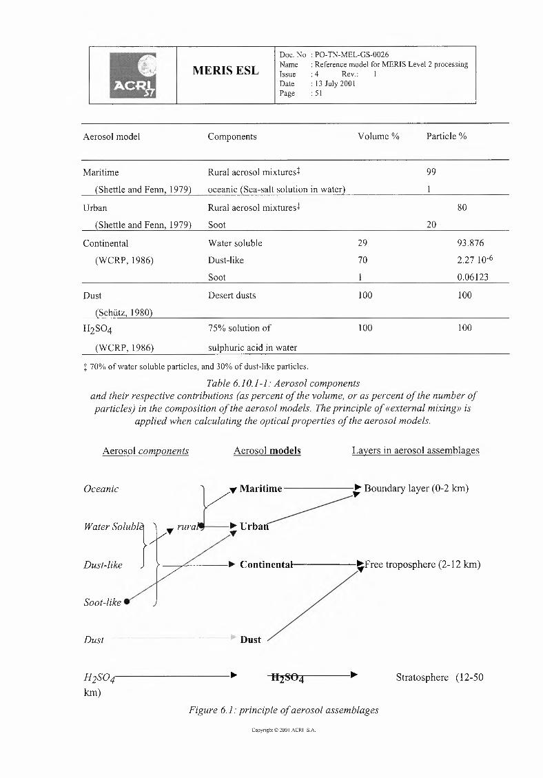
MERIS ESLDoc. No : PO-TN-MEL-GS-0026Name : Reference model for MERIS Level 2 processingIssue : 4 Rev.: IDate : 13 July 200 IPage : 51
Aerosol model Components Volume% Particle%
(Shettle and Fenn, 1979)
Rural aerosol mixtures!
oceanic (Sea-salt solution in water2
99Maritime
Urban Rural aerosol mixturesl
(Shettle and Fenn, 1979) Soot
80
20
29 93.876
70 2.27 10-6
0.06123
100 100
100 100
(WCRP, 1986)
Water soluble
Dust-like
Soot
Continental
Dust Desert dusts
(Schutz, 1980)
H2S04
(WCRP, 1986)
75% solution of
sulphuric acid in water
t 70% of water soluble particles, and 30% of dust-like particles.
Table 6.10.1-1: Aerosol componentsand their respective contributions (as percent of the volume, or as percent of the number ofparticles) in the composition of the aerosol models. The principle of «external mixing» is
applied when calculating the optical properties of the aerosol models.
Aerosol components Aerosol models Layers in aerosol assemblages
Oceanic .: Maritime ~Boundary layer (0-2 km)
.,., rura ~ Urba~Water Solubl}
Dust-like ---,,,£.---~ Continenta ~Free troposphere (2-12 km)
Soot-like
Dust Dust
Stratosphere (12-50
Figure 6.1: principle of aerosol assemblages
Copyright© 200I ACRI S.A.
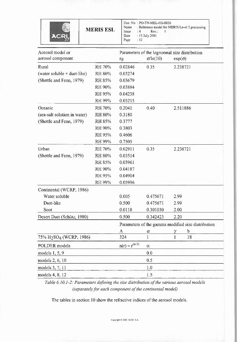
II MERIS ESLDoc. No : PO-TN-MEL-GS-0026Name : Reference model for MERIS Level 2 processingIssue : 4 Rev.: 1
•
Date : 13 July 2001Page : 52
Aerosol model oraerosol component
Parameters of the lognormal size distributionro a/In(10) exp(a)
Rural(water soluble+ dust-like)(Shettle and Fenn, 1979)
RH70%RH80%RH85%RH90%RH95%RH99%
0.02846 0.35 2.2387210.032740.036790.038840.042380.05215
0.40Oceanic(sea-salt solution in water)(Shettle and Fenn, 1979)
RH70%RH80%RH85%RH90%RH95%RH99%
0.20410.31800.37770.38030.46060.7505
2.511886
Urban(Shettle and Fenn, 1979)
RH70%RH80%RH85%RH90%RH95%RH99%
0.029110.035140.039610.041870.049040.05996
0.35 2.238721
Continental (WCRP, 1986)Water solubleDust-likeSoot
0.0050.5000.0118
0.4756710.4756710.301030
2.992.992.00
Desert Dust £Schiltz, 1980) 2.200.500 0.342423
Parameters of the gamma modified size distributionA a Y b
75% H2S04 (WCRP, 1986) 324 1 1 18
POLDER models n(r) ~ r(a-3) amodels 1, 5, 9 0.0models 2, 6, 10 0.5models 3, 7, 11 1.0models 4, 8, 12 1.5
Table 6.10.1-2: Parameters defining the size distribution of the various aerosol models(separately for each component of the continental model)
The tables in section 10 show the refractive indices of the aerosol models.
Copyright© 2001ACRI S.A.
MERIS ESLDoc. No : PO-TN-MEL-GS-0026Name : Reference model for MERIS Level 2 processingIssue : 4 Rev.: 1Date : 13 July 2001Page : 53
6.10.2 -AEROSOL PHASE FUNCTION & SINGLE SCATTERING ALBEDO
Aerosol phase function, extinction and scattering coefficients, single scattering albedo,asymmetry factor shall be computed according to Mie theory, based on the parametersidentified in section 6.10.1 above.
The table in section 11 (divided into 3 parts) summarises the results of Miecomputations. For each aerosol model, and for each wavelength, there are 2 lines : the firstone for the scattering (b) and attenuation (c) coefficients (thus 2 successive values for eachwavelength), the second one for the single scattering albedo (w) and the asymmetry factor (g).
The plots in section 13 show the scattering phase function at 550nm, of the aerosolmodels. A full set of discretised phase functions can be retrieved as a binary file from thefollowing ftp server: ftp.acri. fr, login: meris: password: envisat, file:pub/phase_ functions. tar. z (archive created with the Unix tar utility and compressed bythe Unix compress utility).
6.10.3 - AEROSOL VERTICAL PROFILES
Aerosol assemblages shall be specified by:1. a boundary layer aerosol: model, optical thickness at 560nm, between 0 and 2 km altitude2. a tropospheric layer aerosol: model, optical thickness at 560nm, between 2 and 12 km
altitude3. a stratospheric layer aerosol: model, optical thickness at 560nm, above 12 km altitude
The 33 assemblages used for atmosphere corrections above water are described insection 12 below.
The POLDER models used for atmosphere corrections above land shall be distributedfollowing:
8(z) = 8(0).e -?{,where 8(z) is the optical thickness at altitude z, H the scale height; H = 2 km for all POLDERmodels.
6.11 - REFERENCE ATMOSPHERE
For the purposes of validation and of look-up table computation (i.e. those which donot require variations of the atmosphere properties), a reference atmosphere has been definedwith the following parameters:
Rayleigh scattering as defined in 6.6 above, with a sea level pressure of 1013.25 hPaboundary layer aerosol: maritime model with relative humidity = 90%, 'ta560: 0.2tropospheric, stratospheric aerosols: nonetotal ozone: nonetotal water vapour: nonewind speed: 3 m.s'
Copyright e 200 I ACRI S.i\.
MERIS ESLDoc. No : PO-TN-MEL-GS-0026Name : Reference model for MERIS Level 2 processingIssue : 4 Rev.: IDate : 13 July 200 IPage : 54
7. - Clouds
7.1 -WATERCLOUDS
Cloud types shall be taken from ATBD volume 1, Cloud albedo and optical thickness,section 3.1.2.1. Each cloud type is specified a population of water droplets with a modifiedgamma-function distribution, characterised by its effective radius (µm).
The cloud scattering phase function, extinction and scattering coefficients, shall becomputed according to Mie theory, based on the cloud parameters identified above.
Clouds shall be specified by a type and an extinction coefficient (m") in eachatmosphere layer.
7.2 - CIRRUS CLOUDS
It shall be possible to specify layer(s) of cirrus cloud, whose optical properties:scattering phase function, extinction and scattering coefficients, shall be taken from Brogniezeta!. (1995).
Copyright© 2001ACRI S.A.
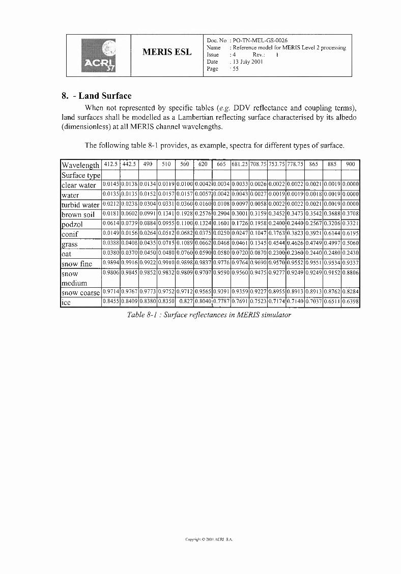
MERIS ESLDoc. No : PO-TN-MEL-GS-0026Name : Reference model for MERIS Level 2 processingIssue : 4 Rev.: 1Date : 13 July 2001Page : 55
8. - Land SurfaceWhen not represented by specific tables (e.g. DDV reflectance and coupling terms),
land surfaces shall be modelled as a Lambertian reflecting surface characterised by its albedo(dimensionless) at all MERIS channel wavelengths.
The following table 8-1 provides, as example, spectra for different types of surface.
Wavelength 412.5 442.5 490 510 560 620 665 681.25 708.75 753.75 778.75 865 885 900
Surface typeclear water 0.0145 0.0138 0.0134 0.0119 0.0100 0.0042 0.0034 0.0033 0.0026 0.0022 0.0022 0.0021 0.0019 0.0000
water 0.0135 0.0135 0.0152 0.0157 0.0157 0.0057 0.0042 0.0043 0.0027 0.0019 0.0019 0.0018 0.0019 0.0000
turbid water 0.0212 0.0238 0.0304 0.0331 0.0360 0.0160 0.0108 0.0097 0.0058 0.0022 0.0022 0.0021 0.0019 0.0000
brown soil 0.0181 0.0602 0.0991 0.1341 0.1928 0.2576 0.2904 0.3001 0.3159 0.3452 0.3473 0.3542 0.3688 0.3708
podzol 0.0614 0.0739 0.0884 0.0955 0.1100 0.1324 0.1601 0.1726 0.1958 0.2400 0.2440 0.2567 0.3206 0.3321
conif 0.0149 0.0156 0.0264 0.0512 0.0682 0.0375 0.0250 0.0247 0.1047 0.3763 0.3823 0.3921 0.6144 0.6195
grass 0.0388 0.0408 0.0435 0.0715 0.1089 0.0662 0.0468 0.0461 0.1345 0.4544 0.4626 0.4749 0.4997 0.5060
oat 0.0380 0.0370 0.0450 0.0480 0.0760 0.0590 0.0580 0.0720 0.0870 0.2300 0.2360 0.2440 0.2480 0.2430
snow fine 0.9894 0.9916 0.9922 0.9910 0.9898 0.9837 0.9776 0.9764 0.9690 0.9570 0.9552 0.9551 0.9534 0.9337
snow 0.9806 0.9845 0.9852 0.9832 0.9809 0.9707 0.9590 0.9560 0.9475 0.9277 0.9249 0.9249 0.9152 0.8806
mediumsnow coarse 0.9714 0.9767 0.9773 0.9752 0.9712 0.9565 0.9391 0.9359 0.9227 0.8955 0.8913 0.8913 0.8762 0.8284
ice 0.8455 0.8409 0.8380 0.8350 0.827 0.8040 0.7787 0.7691 0.7523 0.7174 0.7140 0.7037 0.6511 0.6398
Table 8-1 : Surface reflectances in MERIS simulator
Copyright0 200 I ACRI s.x.

MERIS ESLDoc. No : PO-TN-MEL-GS-0026Name : Reference model for MERIS Level 2 processingIssue : 4 Rev.: 1Date : 13 July 2001Page : 56
9. - Sun irradianceSun irradiance when needed, shall be taken from Thuilier et al. (1998a, 1998b). It shall
be corrected for the day of year according to the following approximate formulae:7t
M = 0.9856.(J-4).-1801E(J)=E0.------
(1-0.01673.cosM)where J is the day of year.
Copyright0 200 I ACRI S.A.
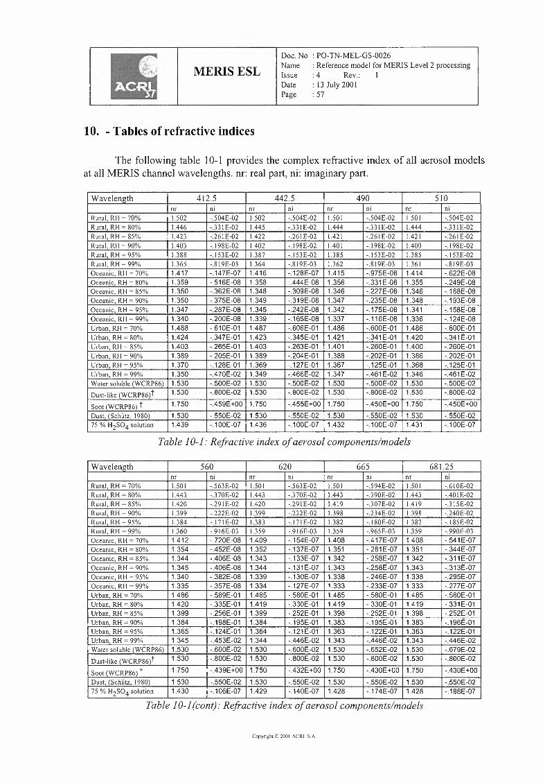
Doc. No : PO-TN-MEL-GS-0026
MERIS ESL NameIssueDatePage
: Reference model for MERIS Level 2 processing: 4 Rev.: 1: 13 July 2001: 57
10. - Tables of refractive indices
The following table 10-1 provides the complex refractive index of all aerosol modelsat all MERIS channel wavelengths. nr: real part, ni: imaginary part.
Wavelength 412.5 442.5 490 510nr ni nr ni nr ni nr ni
Rural, RH= 70% 1.502 -.504E-02 1.502 -.504E-02 1.501 -.504E-02 1.50I -.504E-02Rural, RH= 80% 1.446 -.331E-02 1.445 -.33IE-02 1.444 -.331E-02 1.444 -.331E-02Rural, RH= 85% 1.423 -.261E-02 1.422 -.261E-02 1.421 -.261E-02 1.421 -.261E-02Rural, RH= 90% 1.403 -.!98E-02 1.402 -.!98E-02 1.401 -. I98E-02 1.400 -.I98E-02Rural, RH= 95% 1.388 -.153E-02 1.387 -.I 53E-02 1.385 -. I53E-02 1.385 -.153E-02Rural, RH= 99% 1.365 -.8I9E-03 1.364 -.819E-03 1.362 -.819E-03 1.361 -.819E-03Oceanic, RH= 70% 1.417 -.147E-07 1.416 -.128E-07 1.415 -.975E-08 1.414 -.622E-08Oceanic, RH= 80% 1.359 -.516E-08 1.358 -.444E-08 1.356 -.331E-08 1.355 -.249E-08Oceanic, RH= 85% 1.350 -.362E-08 1.348 -.309E-08 1.346 -.227E-08 1.346 -.188E-08Oceanic, RH= 90% 1.350 -.375E-08 1.349 -.319E-08 1.347 -.235E-08 1.348 -.193E-08Oceanic, RH= 95% 1.347 -.287E-08 1.345 -.242E-08 1.342 -.175E-08 1.341 -.158E-08Oceanic, RH= 99% 1.340 -.200E-08 1.339 -.165E-08 1.337 -.116E-08 1.336 -.124E-08Urban, RH= 70% 1.488 -.61OE-01 1.487 -.606E-01 1.486 -.600E-01 1.486 -.600E-01Urban, RH= 80% 1.424 -.347E-01 1.423 -.345E-01 1.421 -.341E-01 1.420 -.341E-01Urban, RH= 85% 1.403 -.265E-01 1.403 -.263E-01 1.401 -.260E-01 1.400 -.260E-01Urban, RH= 90% 1.389 -.205E-01 1.389 -.204E-01 1.388 -.202E-01 1.386 -.202E-01Urban, RH= 95% 1.370 -.128E-01 1.369 -.127E-01 1.367 -.125E-01 1.368 -.125E-01Urban, RH= 99% 1.350 -.470E-02 1.349 -.466E-02 1.347 -.461E-02 1.346 -.461E-02Water soluble (WCRP86) 1.530 -.500E-02 1.530 -.500E-02 1.530 -.500E-02 1.530 -.500E-02Dust-like(WCRP86)t 1.530 -.800E-02 1.530 -.BOOE-02 1.530 -.800E-02 1.530 -.BOOE-02
Soot (WCRP86)t 1.750 -.459E+OO 1.750 -.455E+OO 1.750 -.450E+OO 1.750 -.450E+OODust, (Schlitz, 1980) 1.530 -.550E-02 1.530 -.550E-02 1.530 -.550E-02 1.530 -.550E-0275 % H2so4 solution 1.439 -.100E-07 1.436 -.100E-07 1.432 -.1OOE-07 1.431 -.100E-07
Table 10-1: Refractive index of aerosol components/models
Wavelength 560 620 665 681.25nr ni nr ni nr Ill nr ni
Rural, RH= 70% 1.501 -.563E-02 1.501 -.563E-02 1.501 -.594E-02 1.501 -.610E-02Rural, RH= 80% 1.443 -.370E-02 1.443 -.370E-02 1.443 -.390E-02 1.443 -.401E-02Rural, RH= 85% 1.420 -.291E-02 1.420 -.291E-02 1.419 -.307E-02 1.419 -.3l5E-02Rural, RH= 90% 1.399 -.222E-02 1.399 -.222E-02 1.398 -.234E-02 1.398 -.240E-02Rural, RH= 95% 1.384 -.171E-02 1.383 -.171E-02 1.382 -.180E-02 1.382 -.l 85E-02Rural, RH= 99% 1.360 -.916E-03 1.359 -.916E-03 1.359 -.965E-03 1.359 -.990E-03Oceanic, RH= 70% 1.412 -.720E-08 1.409 -.154E-07 1.408 -.417E-07 1.408 -.541E-07Oceanic, RH= 80% 1.354 -.452E-08 1.352 -.137E-07 1.351 -.281E-07 1.351 -.344E-07Oceanic, RH= 85% 1.344 -.406E-08 1.343 -.133E-07 1.342 -.258E-07 1.342 -.311E-07Oceanic, RH= 90% 1.345 -.406E-08 1.344 -.131E-07 1.343 -.258E-07 1.343 -.313E-07Oceanic, RH= 95% 1.340 -.382E-08 1.339 -.130E-07 1.338 -.246E-07 1.338 -.295E-07Oceanic,RH = 99% 1.335 -.357E-08 1.334 -.127E-07 1.333 -.233E-07 1.333 -.277E-07Urban, RH = 70% 1.486 -.589E-01 1.485 -.580E-01 1.485 -.580E-01 1.485 -.580E-01Urban, RH= 80% 1.420 -.335E-01 1.419 -.330E-01 1.419 -.330E-01 1.419 -.331E-01Urban, RH= 85% 1.399 -.256E-01 1.399 -.252E-01 1.398 -.252E-01 1.398 -.252E-01Urban, RH= 90% 1.384 -.198E-01 1.384 -.195E-01 1.383 -.195E-01 1.383 -.196E-01Urban, RH= 95% 1.365 -.124E-01 1.364 -.121E-01 1.363 -.122E-01 1.363 -.122E-01Urban, RH= 99% 1.345 -.453E-02 1.344 -.446E-02 1.343 -.446E-02 1.343 -.446E-02Water soluble (WCRP86) 1.530 -.600E-02 1.530 -.600E-02 1.530 -.652E-02 1.530 -.679E-02Dust-like(WCRP86)t 1.530 -.800E-02 1.530 -.800E-02 1.530 -.800E-02 1.530 -.800E-02
Soot (WCRP86)t 1.750 -.439E+OO 1.750 -.432E+OO 1.750 -.430E+OO 1.750 -.430E+OODust, (Schutz, 1980) 1.530 -.550E-02 1.530 -.550E-02 1.530 -.550E-02 1.530 -.550E-0275 % H2so4 solution 1.430 -.106E-07 1.429 -.140E-07 1.428 -.174E-07 1.428 -.188E-07
Table 10-1(cont): Refractive index of aerosol components/models
Copyright <O200 I ACRI SA
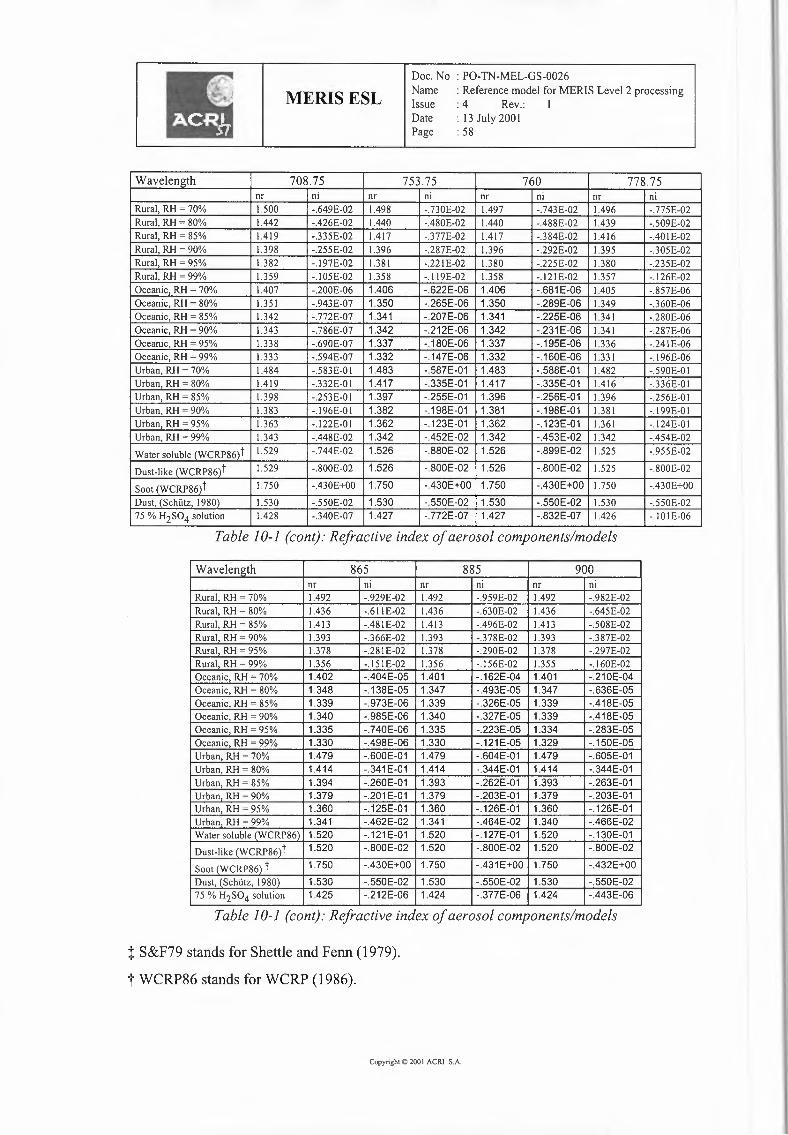
MERIS ESL NameIssueDatePage
: Reference model for MERIS Level 2 processing: 4 Rev.: I: 13 July 2001: 58
Doc. No : PO-TN-MEL-GS-0026
Wavelength 708.75 753.75 760 778.75nr Ill nr ni nr ni nr ni
Rural,RH= 70% 1.500 -.649E-02 1.498 -.730E-02 1.497 -.743E-02 1.496 -.775E-02Rural,RH= 80% 1.442 -.426E-02 1.440 -.480E-02 1.440 -.488E-02 1.439 -.509E-02Rural, RH= 85% 1.419 -.335E-02 1.417 -.377E-02 1.417 -.384E-02 1.416 -.401E-02Rural, RH= 90% 1.398 -.255E-02 1.396 -.287E-02 1.396 -.292E-02 1.395 -.305E-02Rural,RH= 95% 1.382 -.197E-02 1.381 -.221E-02 1.380 -.225E-02 1.380 -.235E-02Rural, RH= 99% 1.359 -.105E-02 1.358 -. l 19E-02 1.358 -.121E-02 1.357 -.126E-02Oceanic,RH= 70% 1.407 -.200E-06 1.406 -.622E-06 1.406 -.681E-06 1.405 -.857E-06Oceanic,RH= 80% 1.351 -.943E-07 1.350 -.265E-06 1.350 -.289E-06 1.349 -.360E-06Oceanic,RH= 85% 1.342 -.772E-07 1.341 -.207E-06 1.341 -.225E-06 1.341 -.280E-06Oceanic,RH= 90% 1.343 -.786E-07 1.342 -.212E-06 1.342 -.231E-06 1.341 -.287E-06Oceanic,RH= 95% 1.338 -.690E-07 1.337 -.180E-06 1.337 -.195E-06 1.336 -.241E-06Oceanic,RH= 99% 1.333 -.594E-07 1.332 -.147E-06 1.332 -.160E-06 1.331 -.196E-06Urban, RH= 70% 1.484 -.583E-Ol 1.483 -.587E-01 1.483 -.588E-01 1.482 -.590E-OlUrban, RH= 80% 1.419 -.332E-Ol 1.417 -.335E-01 1.417 -.335E-01 1.416 -.336E-OlUrban,RH= 85% 1.398 -.253E-Ol 1.397 -.255E-01 1.396 -.256E-01 1.396 -.256E-OlUrban, RH= 90% 1.383 -.l 96E-Ol 1.382 -.198E-01 1.381 -.198E-01 1.381 -.199E-01Urban, RH= 95% 1.363 -.122E-Ol 1.362 -.123E-01 1.362 -.123E-01 1.361 -.124E-01Urban, RH= 99% 1.343 -.448E-02 1.342 -.452E-02 1.342 -.453E-02 1.342 -.454E-02Water soluble (WCRP86)t 1.529 -.744E-02 1.526 -.880E-02 1.526 -.899E-02 1.525 -.955E-02
Dust-like (WCRP86lt 1.529 -.800E-02 1.526 -.800E-02 1.526 -.800E-02 1.525 -.800E-02
Soot (WCRP86)t 1.750 -.430E+OO 1.750 -.430E+OO 1.750 -.430E+OO 1.750 -.430E+OODust, (Schiitz, 1980) 1.530 -.550E-02 1.530 -.550E-02 1.530 -.550E-02 1.530 -.550E-0275% H2so4 solution 1.428 -.340E-07 1.427 -.772E-07 1.427 -.832E-07 1.426 -.IOIE-06
Copyright© 2001ACRI S.A.
Table 10-1 (cont): Refractive index of aerosol components/models
Wavelength 865 885 900nr ni nr ni nr ni
Rural, RH= 70% 1.492 -.929E-02 1.492 -.959E-02 1.492 -.982E-02Rural, RH= 80% 1.436 -.61lE-02 1.436 -.630E-02 1.436 -.645E-02Rural, RH= 85% 1.413 -.481E-02 1.413 -.496E-02 1.413 -.508E-02Rural, RH= 90% 1.393 -.366E-02 1.393 -.378E-02 1.393 -.387E-02Rural, RH= 95% 1.378 -.281E-02 1.378 -.290E-02 1.378 -.297E-02Rural, RH= 99% 1.356 -.151E-02 1.356 -.156E-02 1.355 -.160E-02Oceanic,RH= 70% 1.402 -.404E-05 1.401 -.162E-04 1.401 -.210E-04Oceanic,RH= 80% 1.348 -.138E-05 1.347 -.493E-05 1.347 -.636E-05Oceanic, RH= 85% 1.339 -.973E-06 1.339 -.326E-05 1.339 -.418E-05Oceanic, RH= 90% 1.340 -.985E-06 1.340 -.327E-05 1.339 -.418E-05Oceanic, RH= 95% 1.335 -.740E-06 1.335 -.223E-05 1.334 -.283E-05Oceanic, RH= 99% 1.330 -.498E-06 1.330 -.121 E-05 1.329 -.150E-05Urban, RH= 70% 1.479 -.600E-01 1.479 -.604E-01 1.479 -.605E-01Urban, RH= 80% 1.414 -.341E-01 1.414 -.344E-01 1.414 -.344E-01Urban, RH= 85% 1.394 -.260E-01 1.393 -.262E-01 1.393 -.263E-01Urban, RH= 90% 1.379 -.201E-01 1.379 -.203E-01 1.379 -.203E-01Urban, RH= 95% 1.360 -.125E-01 1.360 -.126E-01 1.360 -.126E-01Urban, RH= 99% 1.341 -.462E-02 1.341 -.464E-02 1.340 -.466E-02Water soluble (WCRP86) 1.520 -.121E-01 1.520 -.127E-01 1.520 -.130E-01Dust-like(WCRP86)t 1.520 -.800E-02 1.520 -.800E-02 1.520 -.800E-02
Soot (WCRP86)t 1.750 -.430E+OO 1.750 -.431 E+OO 1.750 -.432E+OODust, (Schiitz, 1980) 1.530 -.550E-02 1.530 -.550E-02 1.530 -.550E-0275% H1S04 solution 1.425 -.212E-06 1.424 -.377E-06 1.424 -.443E-06
Table 10-1 (cont): Refractive index of aerosol components/models
t S&F79 stands for Shettle and Fenn (1979).
t WCRP86 stands for WCRP (1986).

Doc. No : PO-TN-MEL-GS-0026Name : Reference model for MERIS Level 2 processingIssue : 4 Rev.: lDate : 13 July 2001Page : 59
MERIS ESL
model no nr ni1 1.33 02 Idem Idem3 Idem Idem4 Idem Idem5 1.44 06 Idem Idem7 Idem Idem8 Idem Idem9 1.55 -0.00810 1.55 -0.006511 1.55 -0.00512 1.55 -0.0023
Table I 0-2 : Refractive index of land aerosol modelsNote: the refractive indices in table 10-2 are independent of wavelength.
Copyright© 200I ACRI S.A.

Doc. No : PO-TN-MEL-GS-0026
MERIS ESL NameIssueDatePage
: Reference model for MERIS Level 2 processing: 4 Rev.: I: 13 July 2001: 60
11. - Tables of aerosols optical properties (ATBD 2.7)
For each aerosol model, and for each wavelength, there are 2 lines : the first one for thescattering (b) and attenuation (c) coefficients (thus 2 successive values for each wavelength),the second one for the single scattering albedo (w) and the asymmetry factor (g).
'A 412.5 442.5 490 510 560H2S04 .148329 .148330+00 .139728 .139730+00 .126184 .126180+00 .120614 .120610+00 .107559 .107560+00
H2S04 1.000000 .739110+00 1.000000 .738550+00 1.000000 .735050+00 1.000000 .732490+00 1.000000 .724010+00
con ti .000683 .756570·03 .000632 .700700-03 .000563 .625660-03 .000537 .596880-03 .000474 .531120-03
con ti .902636 .641010+00 .901856 .640380+00 .900226 .639450+00 .899168 .638610+00 .891938 .636920+00
des50 4.850898 .616570+01 4.939096 .620820+01 5.065333 .627110+01 5.116927 .629810+01 5.240319 .636440+01
des50 .786751 .809230+00 .795575 .802460+00 .807732 .792990+00 .812458 .789190+00 .823385 .780330+00
mar70 .030204 .306500-01 .029395 .298050-01 .028263 .286250-01 .027819 .281640-01 .026822 .271630-01
mar70 .985458 .723490+00 .986277 .722500+00 .987366 .721470+00 .987775 .721420+00 .987446 .720570+00
mar80 .057857 .582950-01 .056887 .572890-01 .055569 .559260-01 .055006 .553450-01 .053836 .541730-01
mar80 .992492 .773520+00 .992985 .772830+00 .993629 .772160+00 .993863 .773040+00 .993767 .772530+00
mar85 .079569 .800590-01 .078356 .788050-01 .076715 .771150-01 .076006 .763870-01 .074549 .749280-01
mar85 .993892 .786400+00 .994294 .785770+00 .994818 .784690+00 .995009 .785040+00 .994933 .784470+00
mar90 .083267 .837010-01 .081929 .823280-01 .079985 .803390-01 .079195 .795330-01 .077586 .779240-01
mar90 .994824 .789350+00 .995160 .787740+00 .995590 .787110+00 .995753 .786480+00 .995661 .785140+00
mar95 .114715 .115150+00 .113103 .113500+00 .110920 .111280+00 .110126 .110470+00 .108099 .108440+00
mar95 .996227 .801570+00 .996476 .800790+00 .996804 .799380+00 .996926 .798380+00 .996870 .797530+00
mar99 .265249 .265690+00 .263162 .263560+00 .260031 .260390+00 .258592 .258930+00 .255927 .256270+00
mar99 .998360 .825270+00 .998476 .823970+00 .998625 .822810+00 .998680 .823260+00 .998661 .821280+00
urb70 .010416 .144530-01 .009725 .134910-01 .008772 .121760-01 .008397 .116740-01 .007564 .105150-01
urb70 .720650 .710940+00 .720892 .704230+00 .720470 .694270+00 .719327 .690070+00 .719420 .679630+00
urb80 .017550 .219360-01 .016437 .205130-01 .014856 .185210-01 .014213 .177340-01 .012853 .160130-01
urb80 .800071 .743990+00 .801320 .738590+00 .802124 .730850+00 .801451 .727750+00 .802615 .718780+00
urb85 .024571 .295160-01 .023168 .277640-01 .021070 .252010-01 .020211 .241790-01 .018333 .218910-01
urb85 .832462 .758240+00 .834441 .753080+00 .836095 .746410+00 .835894 .743750+00 .837461 .736230+00
urb90 .028832 .335120-01 .027208 .315520-01 .024837 .287360-01 .023776 .275160-01 .021529 .248700-01
urb90 .860340 .765060+00 .862324 .760340+00 .864306 .753810+00 .864095 .751910+00 .865669 .745460+00
urb95 .044996 .499000-01 .042636 .471700-01 .039165 .432160-01 .037920 .418150-01 .034508 .380000-01
urb95 .901731 .777770+00 .903877 .774610+00 .906263 .770020+00 .906867 .767080+00 .908106 .762650+00
urb99 .109992 .115290+00 .105894 .110790+00 .099538 .103910+00 .096809 .101000+00 .090518 .942570-01
urb99 .954029 .792200+00 .955808 .790890+00 .957931 .789010+00 .958493 .788290+00 .960330 .785290+00
Table 11-1: Optical properties of aerosol models
Copyright© 2001ACRI S.A.
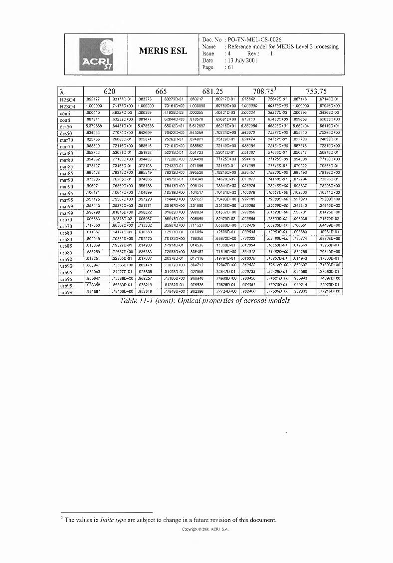
Doc. No : PO-TN-MEL-GS-0026
MERIS ESL NameIssueDatePage
: Reference model for MERIS Level 2 processing: 4 Rev.: 1: 13 July 2001: 61
/... 620 665 681.25 708.75j 753.75H2S04 .093177 .931770-01 .083373 .833730-01 .080217 .802170-01 .075642 .756420-01 .067148 .671480-01
H2S04 1.000000 .711770+00 1.000000 .701610+00 1.000000 .697690+00 1.000000 .691730+00 1.000000 .679460+00
con ti .000410 .462270-03 .000369 .418380-03 .000355 .404010-03 .000334 .382630-03 .000295 .343650-03
con ti .887941 .632320+00 .881477 .628440+00 .878570 .626810+00 .873113 .624600+00 .859658 .620550+00
des50 5.379658 .644310+01 5.478536 .650120+01 5.512597 .652160+01 5.562956 .655260+01 5.659404 .661190+01
des SO .834953 .770740+00 .842699 .764220+00 .845289 .762040+00 .848970 .758870+00 .855940 .752980+00
mar70 .025765 .260650-01 .025074 .253630-01 .024821 .251080-01 .024474 .247620-01 .023799 .240980-01
mar70 .988500 .721160+00 .988616 .721010+00 .988562 .721490+00 .988354 .721540+00 .987578 .723190+00
mar80 .052733 .530310-01 .051928 .522150-01 .051723 .520100-01 .051367 .516550-01 .050617 .509180-01
mar80 .994382 .771650+00 .994489 .772200+00 .994490 .771250+00 .994416 .771250+00 .994098 .771900+00
mar85 .073127 .734630-01 .072108 .724320-01 .071856 .721800-01 .071389 .717150-01 .070522 .708630-01
mar85 .995428 .783180+00 .995519 .783120+00 .995520 .782100+00 .995457 .782200+00 .995196 .781930+00
mar90 .075906 .762050-01 .074685 .749750-01 .074340 .746290-01 .073877 .741680-01 .072794 .730980-01
mar90 .996071 .783690+00 .996138 .784130+00 .996134 .783440+00 .996078 .782450+00 .995837 .782930+00
mar95 .106171 .106470+00 .104899 .105190+00 .104517 .104810+00 .103878 .104170+00 .102806 .103110+00
mar95 .997175 .795670+00 .997229 .794440+00 .997227 .794030+00 .997185 .793800+00 .997020 .793090+00
mar99 .253413 .253720+00 .251371 .251670+00 .251086 .251380+00 .250386 .250690+00 .248840 .249160+00
mar99 .998798 .818150+00 .998822 .818050+00 .998824 .816370+00 .998806 .815230+00 .998731 .814250+00
urb70 .006663 .928780-02 .006067 .850430-02 .005869 .824790-02 .005585 .788330-02 .005036 .718790-02
urb70 .717350 .668070+00 .713362 .659610+00 .711527 .656680+00 .708479 .652360+00 .700551 .644590+00
urb80 .011367 .141740-01 .010389 .129930-01 .010064 .126060-01 .009598 .120530-01 .008683 .109810-01
urb80 .802019 .708810+00 .799570 .701320+00 .798355 .698720+00 .796322 .694860+00 .790774 .688080+00
urb85 .016369 .195270-01 .014983 .179140-01 .014536 .173980-01 .013894 .166600-01 .012669 .152580-01
urb85 .838259 .726870+00 .836383 .720530+00 .835487 .718160+00 .834012 .714620+00 .830285 .708100+00
urb90 .019251 .222050-01 .017637 .203780-01 .017116 .197940-01 .016370 .189570-01 .014943 .173630-01
urb90 .866947 .736660+00 .865478 .730720+00 .864712 .728470+00 .863522 .725120+00 .860637 .718930+00
urb95 .031043 .341270-01 .028635 .314930-01 .027856 .306470-01 .026733 .294280-01 .024560 .270800-01
urb95 .909647 .755880+00 .909257 .751000+00 .908948 .749080+00 .908426 .746210+00 .906943 .740970+00
urb99 .083358 .866630-01 .078219 .812820-01 .076536 .795260-01 .074081 .769700-01 .069214 .719230-01
urb99 .961867 .781360+00 .962319 .778480+00 .962398 .777240+00 .962460 .775360+00 .962332 .772160+00
Table 11-1 (cont): Optical properties of aerosol models
3 The values in Italic type are subject to change in a future revision of this document.Copyright© 200I ACRI SA

Doc. No : PO-TN-MEL-GS-0026
MERIS ESL NameIssueDatePage
: Referencemodel forMERISLevel 2 processing: 4 Rev.: 1: 13July 2001: 62
A. 760 778.754 865 890 900H2S04 .066022 .660220-01 .063550 .635500-01 .050916 .509160-01 .047788 .477890-01 .046675 .466750-01
H2S04 .999999 .677590+00 1.000000 .673690+00 .999999 .648920+00 .999997 .641930+00 .999997 .639020+00
con ti .000291 .338810-03 .000280 .328020-03 .000225 .272280-03 .000213 .259960-03 .000209 .255300-03
con ti .857921 .619790+00 .853615 .618420+00 .826760 .608430+00 .820058 .605320+00 .817381 .604150+00
des50 5.672920 .662000+01 5.702191 .663880+01 5.866978 .674380+01 5.909829 .677120+01 5.926989 .678280+01
des SO .856938 .752190+00 .858914 .750470+00 .869978 .741200+00 .872792 .738900+00 .873822 .738000+00
mar70 .023697 .239970-01 .023520 .238230-01 .022468 .227830-01 .022219 .225390-01 .022113 .224340-01
mar70 .987500 .723390+00 .987288 .723790+00 .986172 .726480+00 .985816 .727070+00 .985662 .727480+00
mar80 .050522 .508240-01 .050304 .506090-01 .049185 .495050-01 .048913 .492380-01 .048822 .491480-01
mar80 .994067 .771970+00 .993978 .772420+00 .993548 .774170+00 .993406 .775020+00 .993353 .775020+00
mar85 .070405 .707460-01 .070101 .704470-01 .068762 .691250-01 .068455 .688240-01 .068346 .687180-01
mar85 .995171 .781940+00 .995101 .782350+00 .994747 .783430+00 .994633 .783470+00 .994590 .783450+00
mar90 .072670 .729760-01 .072381 .726900-01 .070823 .711490-01 .070498 .708300-01 .070389 .707240-01
mar90 .995813 .782800+00 .995748 .782890+00 .995418 .783690+00 .995305 .783350+00 .995265 .783530+00
mar95 .102614 .102920+00 .102366 .102680+00 .100757 .101090+00 .100379 .100720+00 .100151 .100490+00
mar95 .997006 .793030+00 .996963 .792270+00 .996736 .791840+00 .996652 .791610+00 .996619 .792690+00
mar99 .248665 .248980+00 .248109 .248430+00 .246070 .246420+00 .245582 .245940+00 .245419 .245780+00
mar99 .998724 .814000+00 .998703 .814110+00 .998596 .812460+00 .998539 .812080+00 .998517 .812210+00
urb70 .004965 .709780-02 .004804 .689500-02 .003992 .586450-02 .003805 .562770-02 .003733 .553670-02
urb70 .699532 .643390+00 .696767 .641130+00 .680769 .627030+00 .676164 .622970+00 .674303 .621360+00
urb80 .008567 .108440-01 .008325 .105570-01 .006963 .895990-02 .006651 .859490-02 .006531 .845460-02
urb80 .790077 .686990+00 .788515 .684670+00 .777071 .672190+00 .773787 .668500+00 .772451 .667030+00
urb85 .012466 .150290-01 .012129 .146430-01 .010257 .125070-01 .009782 .119720-01 .009614 .117810-01
urb85 .829429 .707520+00 .628296 .705370+00 .820083 .693610+00 .817115 .690600+00 .816075 .689240+00
urb90 .014705 .171000-01 .014313 .166610-01 .012128 .142260-01 .011616 .136590-01 .011418 .134410-01
urb90 .859943 .718420+00 .859063 .716370+00 .852546 .705170+00 .850411 .701900+00 .849539 .700590+00
urb95 .024272 .267690-01 .023670 .261170-01 .020272 .224570-01 .019470 .215990-01 .019160 .212690-01
urb95 .906747 .740140+00 .906295 .738350+00 .902670 .728700+00 .901403 .725810+00 .900883 .724660+00
urb99 .068563 .712470-01 .067190 .698240-01 .059382 .617490-01 .057447 .597530-01 .056502 .587810-01
urb99 .962318 .771600+00 .962271 .770410+00 .961677 .763660+00 .961418 .761600+00 .961223 .761320+00
Table 11-1 (cont): Optical properties of aerosol models
4 The values in Italic type are subject to change in a future revision of this document.Copyright© 2001ACRI S.A.

MERIS ESLDoc. No : PO-TN-MEL-GS-0026Name : Reference model for MERIS Level 2 processingIssue : 4 Rev.: IDate : 13 July 2001Page : 63
12. - Tables describing the aerosol assemblages (ATBD 2.7)
Table 12-1 below describes the aerosol assemblages used when defining and testingthe MERIS atmospheric corrections over Case 1 waters. For the 33 assemblages but the firstone, the stratosphere contains the H2S04 aerosol, with ra(550) = 0.005. For assemblage #0,the stratosphere is aerosol-free.
Assemblage Boundary layer (0-2 km) Free troposphere (2-12 km)#
0 Maritime aerosol model (S&F79) Aerosol-freeRH=99%r3(550) in {0.03, 0.1, 0.3, 0.5, 2}
1 Maritime aerosol model (S&F79) Continental aerosol (WCRP, 1986)RH=70% ra(550) = 0.025ra(550) in {0.03, 0.1, 0.3, 0.5, 2}
2 Maritime aerosol model (S&F79) Continental aerosol (WCRP, 1986)RH=80% Ta(550)= 0.025ra(550) in {0.03, 0.1, 0.3, 0.5, 2}
3 Maritime aerosol model (S&F79) Continental aerosol (WCRP, 1986)RH=95% 'fa(550) = 0.025ra(550) in {0.03, 0.1, 0.3, 0.5, 2}
4 Maritime aerosol model (S&F79) Continental aerosol (WCRP, 1986)RH=99% Ta(550)= 0.025ra(550) in {0.03, 0.1, 0.3, 0.5, 2}
5 Urban aerosol model (S&F79) Continental aerosol (WCRP, 1986)RH=70% ra(550) = 0.025r3(550) in {0.03, 0.1, 0.3, 0.5, 2}
6 Urban aerosol model (S&F79) Continental aerosol (WCRP, 1986)RH= 80% 'fa(550) = 0.025ra(550) in {0.03, 0.1, 0.3, 0.5, 2}
7 Urban aerosol model (S&F79) Continental aerosol (WCRP, 1986)RH=95% Ta(550)= 0.025ra(550) in {0.03, 0.1, 0.3, 0.5, 2}
8 Urban aerosol model (S&F79) Continental aerosol (WCRP, 1986)RH =99% Ta(550)= 0.025ra(550) in {0.03, 0.1, 0.3, 0.5, 2}
Table 12-1: Aerosol assemblages used in atmosphere corrections above ocean
CopyrightO 2001ACRI SA

MERIS ESLDoc. No : PO-TN-MEL-GS-0026Name : Reference model for MERIS Level 2 processingIssue : 4 Rev.: 1Date : 13 July 2001Page : 64
9 Maritime aerosol model (S&F79) Continental aerosol (WCRP, 1986)RH=70% fa(550) = 25% of ftropo
ftropo(550)• in {0.05, 0.2, 0.5, 0.8, 2.}IO Maritime aerosol model (S&F79) Continental aerosol (WCRP, 1986)
RH=70% fa(550) = 50% of ftropoftropo(550) in {0.05, 0.2, 0.5, 0.8, 2.}
11 Maritime aerosol model (S&F79) Continental aerosol (WCRP, 1986)RH=70% fa(550) = 75% of 't'tropoftropo(550) in {0.05, 0.2, 0.5, 0.8, 2.}
12 Maritime aerosol model (S&F79) Continental aerosol (WCRP, 1986)RH=80% fa(550) = 25% of ftropoftrop0(550) in {0.05, 0.2, 0.5, 0.8, 2.}
13 Maritime aerosol model (S&F79) Continental aerosol (WCRP, 1986)RH=80% fa(550) = 50% of ftropoftropo(550) in {0.05, 0.2, 0.5, 0.8, 2.}
14 Maritime aerosol model (S&F79) Continental aerosol (WCRP, 1986)RH=80% fa(550) = 75% of ftropoftropo(550) in {0.05, 0.2, 0.5, 0.8, 2.}
15 Maritime aerosol model (S&F79) Continental aerosol (WCRP, 1986)RH=95% fa(550) = 25% of ftropoftropo(550) in {0.05, 0.2, 0.5, 0.8, 2.}
16 Maritime aerosol model (S&F79) Continental aerosol (WCRP, 1986)RH=95% 'X'a(550)= 50% of 'X'tropoftropo(550) in {0.05, 0.2, 0.5, 0.8, 2.}
17 Maritime aerosol model (S&F79) Continental aerosol (WCRP, 1986)RH=95% 'X'a(550)= 75% of 't'tropoftrop0(550) in {0.05, 0.2, 0.5, 0.8, 2.}
18 Maritime aerosol model (S&F79) Continental aerosol (WCRP, 1986)RH=99% 'X'a(550)= 25% of 't'tropoftropo(550) in {0.05, 0.2, 0.5, 0.8, 2.}
19 Maritime aerosol model (S&F79) Continental aerosol (WCRP, 1986)RH=99% fa(550) = 50% of 't'tropoftrop0(550) in {0.05, 0.2, 0.5, 0.8, 2.}
20 Maritime aerosol model (S&F79) Continental aerosol (WCRP, 1986)RH=99% 'X'a(550)= 75% of 't'tropoftrop0(550) in {0.05, 0.2, 0.5, 0.8, 2.}
Table 12-1(cont): Aerosol assemblages used in atmosphere corrections above ocean
Copyright© 200I ACRI S.A.

MERIS ESLDoc. No : PO-TN-MEL-GS-0026Name : Reference model for MERIS Level 2 processingIssue : 4 Rev.: 1Date : 13 July 2001Page : 65
21 Maritime aerosol model (S&F79) Desert dust (Schiltz, 1980)RH=70% "ra(550)= 25% of Ttropo"rtrop0(550)in {0.05, 0.2, 0.5, 0.8, 2.}
22 Maritime aerosol model (S&F79) Desert dust (Schiltz, 1980)RH=70% "ra(550)= 50% of TtropoTtrop0(550) in {0.05, 0.2, 0.5, 0.8, 2.}
23 Maritime aerosol model (S&F79) Desert dust (Schiltz, 1980)RH=70% "ra(550)= 75% of "rtropo"rtrop0(550)in {0.05, 0.2, 0.5, 0.8, 2.}
24 Maritime aerosol model (S&F79) Desert dust (Schiltz, 1980)RH=80% "ra(550)= 25% of "rtropoTtrop0(550) in {0.05, 0.2, 0.5, 0.8, 2.}
25 Maritime aerosol model (S&F79) Desert dust (Schiltz, 1980)RH=80% "ra(550)= 50% of "rtropoTtrop0(550) in {0.05, 0.2, 0.5, 0.8, 2.}
26 Maritime aerosol model (S&F79) Desert dust (Schiltz, 1980)RH= 80% "ra(550)= 75% of TtropoTtrop0(550) in {0.05, 0.2, 0.5, 0.8, 2.}
27 Maritime aerosol model (S&F79) Desert dust (Schiltz, 1980)RH=95% "ra(550)= 25% of TtropoTtrop0(550) in {0.05, 0.2, 0.5, 0.8, 2.}
28 Maritime aerosol model (S&F79) Desert dust (Schiltz, 1980)RH=95% "ra(550)= 50% of TtropoTtrop0(550) in {0.05, 0.2, 0.5, 0.8, 2.}
29 Maritime aerosol model (S&F79) Desert dust (Schiltz, 1980)RH=95% "ra(550)= 75% of 'ltropoTtropo(550) in {0.05, 0.2, 0.5, 0.8, 2.}
30 Maritime aerosol model (S&F79) Desert dust (Schiltz, 1980)RH=99% "ra(550)= 25% of "rtropoTtrop0(550) in {0.05, 0.2, 0.5, 0.8, 2.}
31 Maritime aerosol model (S&F79) Desert dust (Schiltz, 1980)RH=99% "ra(550)= 50% of TtropoTtrop0(550) in {0.05, 0.2, 0.5, 0.8, 2.}
32 Maritime aerosol model (S&F79) Desert dust (Schiltz, 1980)RH=99% "ra(550)= 75% of TtropoTtrop0(550) in {0.05, 0.2, 0.5, 0.8, 2.}
• : NOTE: Ttropo stands now for the whole troposphere (i.e., 0-12 km), while ra was only forthe boundary layer in cases 1 to 8.
Table 12-1 (cont): Aerosol assemblages used in atmosphere corrections above ocean
Copyright© 200I ACRI SA

II- }.
-Doc. No : PO-TN-MEL-GS-0026Name : Reference model for MERIS Level 2 processingIssue : 4 Rev.: 1Date : 13 July 2001Page : 66
13. - Aerosol phase functionsThe figures below show the aerosol scattering phase function at the wavelength
550nm, for the aerosol models. Figure 13-1 shows the aerosol models from ATBD 2.7, figure13-2 the models from ATBD 2.15.
MERIS ESL
IO•~ I II I I I I II I I 1! I I I II I I I I II JI II!!! II I I 1 ! 10-"i! I,, I I I I,, I I,, I I I,,! t I I II,, II 11I 11I I I I 10·10 30 60 90 120 150 180 0 30 60 90 120 150 180 0 30 60 90 120 150 180
9 9 9101 lOl 1Ol
i i i i iICon~e,tal I I lnes~rt dtst I I lvo~ank lash II I II I I I I 101 -1-·-t--·1--1--t·- 101 -1-·-t--·1--1--t·-
10 I l:\-1-·-t--·1--1--t·- I I I I I I I I I II I I I I I I I I I I I I I I
I I I I I I I I I I I I I II I I I 10' -4---~--+--l---1-·- 10' -4---~--+--l---1-·-i i i i i i i i i i i i i i
10° i,..-~--~---L--l---1--- I I I I I I I I I. I I I I I I I I I I Ii i i 10°
_L_.J __ i__l__10°
L_.J __ i__l__I I I I I I I I
I I I ! I !10· 0 1:---j-·-t--·+--i--+----:l i i i i i i
I10·0 --,---r-·T -- 10·0
i i iI I II I I
10-';t I II I I I! 11 I I 1! I I I II! 1 I I !I! 1 11 1 1) II 1 I I! 10-1 10-10 30 60 90 120 150 180 0 30 60 90 120 150 180 0 30 60 90 120 150 180
9 9 9
Figure 13-1: Scattering phase functions for the aerosol models of ATBD 2. 7
10'
10·1
Copyright© 200I ACRI S.A.
Iii Doc. No : PO-TN-MEL-GS-0026
MERIS ESL Name : Reference model for MERIS Level 2 processingIssue : 4 Rev.: IDate : 13 July 2001-Page : 67
Figure 13-2: Scattering phase functions for the aerosol models of ATBD 2.15
Copyright© 2001ACRI SA

MERIS ESLDoc.No : PO-TN-MEL-GS-0026Name : Referencemodel forMERISLevel 2 processingIssue : 4 Rev.: 1Date : 13July 200IPage : 68
14. - Spectral dependency of aerosol optical thickness
14.1 -AEROSOL ASSEMBLAGES (ATM. COR. ABOVEWATER)
For the 33 aerosol assemblages listed in table 12-1 above, the spectral dependency of opticalthickness is tabulated at the first 13 bands and at 5 optical thicknesses in table 14-1 below.The line labelled ta(560) or 'ttropo(560)refers to the optical thickness of the boundary layer +tropospheric aerosol at 560nm (see table 12-1). The values in Italic type are subject to changein a future revision of this document.
Spectral dependency of optical thickness for assemblage 0'ta(560) 0.03 0.1 0.3 0.5 2.0
412 0.031100001 0.103400002 0.310299882 0.516999986 2.06829992443 0.0307 0.102499901 0.307799965 0.512899897 2.051899806490 0.030400001 0.101399998 0.303999894 0.506700002 2.027200022510 0.030300001 0.100799904 0.302399884 0.50400001 2.015899937560 0.029899999 0.0998 0.299199905 0.498699886 1.99510003620 0.0296 0.098700005 0.296200007 0.493799886 1.975200006665 0.029400001 0.097900005 0.293799997 0.489799884 1.95919986681 0.029400001 0.097799995 0.293599979 0.4892999 1.956999858
708.75 0.029300001 0.097599998 0.292800007 0.487899914 1.951500054753 0.028999999 0.096899998 0.290999878 0.484899999 1.939700053761 0.028999999 0.096899998 0.290699988 0.484600019 1.938399953
778.75 0.028999999 0.0968 0.290199875 0.483500018 1.934099879865 0.0288 0.096 0.2878 0.4794999 1.9184
Spectral dependency of optical thickness for assemblage 1'ta(560) 0.03 0.1 0.3 0.5 2.0
412 0.075099999 0.153500006 0.377499891 0.601599877 2.282000106443 0.071300001 0.147499991 0.365299902 0.583299882 2.217200059490 0.065899999 0.139299903 0.348400002 0.557799867 2.127100003510 0.0638 0.135900004 0.341699994 0.547499985 2.091499975560 0.059000002 0.128499896 0.327099987 0.525600028 2.014900038620 0.054200003 0.120800003 0.311299989 0.501899992 1.930899942665 0.050900003 0.115700002 0.301099903 0.486400024 1.876899872681 0.049700002 0.114000006 0.297500019 0.481099909 1.857499918
708.75 0.0483 0.111599899 0.292599987 0.47369998 1.831199946753 0.045200001 0.106799896 0.282999883 0.459099978 1.780400008761 0.045000005 0.106399901 0.281799985 0.457099987 1.772799944
778.75 0.0441 0.104999902 0.279199973 0.453199986 1.759300027865 0.0398 0.0981 0.2646999 0.4311999 1.6803
Table I 4-1: Spectral dependency of aerosol optical thickness
Copyright© 2001ACRI S.A.

MERIS ESLDoc.No : PO-TN-MEL-GS-0026Name : Referencemodel forMERISLevel 2 processingIssue : 4 Rev.: IDate : 13July 2001Page : 69
Spectral dependency of optical thickness for assemblage 2'ta(560) 0.03 0.1 0.3 0.5 2.0
412 0.073600001 0.148699898 0.362999872 0.577199991 2.184099819443 0.070100001 0.143999991 0.354600015 0.565099998 2.144999883490 0.065499996 0.137499998 0.343100002 0.548699901 2.090799928510 0.063399997 0.134599901 0.338200001 0.541700023 2.0678560 0.059099996 0.128700008 0.32759998 0.526400012 2.017799944620 0.054900002 0.123099907 0.318099986 0.512999883 1.975299817665 0.051799999 0.118799995 0.310200005 0.501899894 1.93819988681 0.050899999 0.117900002 0.309099974 0.500299864 1.934399963
708.75 0.049600002 0.115699908 0.305099899 0.494599887 1.914999888753 0.046799998 0.112399904 0.299599983 0.486799876 1.890799887761 0.046599997 0.112099898 0.298799893 0.485799981 1.887299975
778.75 0.0458 0.110600005 0.295999986 0.481300005 1.871799994865 0.0421 0.1053999 0.2867 0.4677 1.8264
Spectral dependency of optical thickness for assemblage 3'ta(560) 0.03 0.1 0.3 0.5 2.0
412 0.073299994 0.147300004 0.358999987 0.570500023 2.157600053443 0.069799996 0.142800003 0.351399875 0.560099893 2.124399954490 0.065199997 0.136899991 0.341300015 0.545799917 2.079500044510 0.063299995 0.134499898 0.337500011 0.540400028 2.063000117560 0.059099996 0.128999996 0.328299902 0.527499976 2.022100073620 0.054999999 0.123399899 0.3191 0.514699874 1.982300067665 0.051899999 0.1196999 0.312900001 0.506199999 1.956100122681 0.050999999 0.118500007 0.311100012 0.503799917 1.948300167
708.75 0.049899999 0.116900005 0.308299893 0.499599928 1.935500094753 0.047299996 0.113499908 0.30299999 0.492499919 1.913800047761 0.046899997 0.1130999 0.302399915 0.491400032 1.909999958
778.75 0.046199996 0.112299899 0.300999908 0.489700023 1.904900073865 0.0428 0.1077 0.2935 0.4793999 1.8725
Spectral dependency of optical thickness for assemblage 4'ta(560) 0.03 0.1 0.3 0.5 2.0
412 0.0726 0.144899903 0.351799989 0.558499846 2.109800179443 0.069300004 0.1410999 0.346399994 0.551499895 2.090500142490 0.065000002 0.135999905 0.338599863 0.541299891 2.061800052510 0.063199998 0.13369989 0.335299994 0.536899944 2.048800079560 0.059200003 0.129099994 0.328499984 0.527999861 2.024400035620 0.055200003 0.124299995 0.321799895 0.519399997 2.000799952665 0.052400004 0.120899893 0.316799969 0.512799932 1.982200098681 0.051600005 0.119999894 0.31579999 0.511500016 1.979200099
708.75 0.050400004 0.118699903 0.313899882 0.509000023 1.972599987753 0.047800001 0.115699899 0.309799907 0.503699992 1.958499986761 0.047600005 0.115499996 0.309299992 0.503199852 1.957000112
778.75 0.046900001 0.114699903 0.308099959 0.501399856 1.952000115865 0.0437 0.1108999 0.3027 0.4943999 1.9333Table 14-1: Spectral dependency of aerosol optical thickness (cont.)
Copyright © 200 I ACRI SA

MERIS ESLDoc. No : PO-TN-MEL-GS-0026Name : Reference model for MERIS Level 2 processingIssue : 4 Rev.: 1Date : 13 July 2001Page :70
Spectral dependency of optical thickness for assemblage 5't.(560) 0.03 0.1 0.3 0.5 2.0
412 0.081800002 0.176100004 0.445499963 0.714799992 2.734400171443 0.076300006 0.16419991 0.415599983 0.666899961 2.552200237490 0.068700002 0.148100012 0.374799918 0.601800015 2.303200016510 0.0656 0.141699997 0.359200003 0.576699971 2.207999935560 0.058699999 0.127199908 0.323100005 0.518999865 1.988400082620 0.051500002 0.112099998 0.285100001 0.458299909 1.756000116665 0.0468 0.102200006 0.260599995 0.419099914 1.607600002681 0.045300002 0.098999998 0.252700007 0.406300023 1.5590001 09
708.75 0.043200001 0.094600001 0.241399997 0.388299926 1.489900013753 0.038800001 0.085799999 0.219599893 0.353700007 1.358000072761 0.038499999 0.084800002 0.217 0.349200008 1.341000007
778.75 0.037099999 0.082099997 0.210600007 0.338999997 1.302600058865 0.0312 0.0695 0.1788 0.2879999 1.1076
Spectral dependency of optical thickness for assemblage 6'ta(560) 0.03 0.1 0.3 0.5 2.0
412 0.0817 0.17580001 0.444200015 0.71269988 2.726299822443 0.076200001 0.164199904 0.41519993 0.66630002 2.549199855490 0.068700002 0.148000006 0.374599914 0.601299992 2.301500104510 0.065500002 0.141500007 0.35849993 0.575499905 2.20339977560 0.058700003 0.127199907 0.3232 0.519200021 1.989299896620 0.051700002 0.11230001 0.285800014 0.459199907 1.760299991665 0.046900002 0.102500003 0.261500004 0.420599907 1.613399873681 0.045400001 0.099300003 0.253600005 0.407900008 1.56509993
708.75 0.0433 0.094800011 0.242400016 0.389899917 1.496299949753 0.038900002 0.086000006 0.220399895 0.354799879 1.362799946761 0.038600002 0.085000003 0.2177 0.350499986 1.34579998
778.75 0.037200003 0.082599999 0.211699904 0.340999978 1.309999858865 0.0314 0.0698 0.1794 0.2890999 1.1116
Spectral dependency of optical thickness for assemblage 71:3(560) 0.03 0.1 0.3 0.5 2.0
412 0.080200001 0.170499994 0.428599909 0.686599991 2.622100129443 0.075199994 0.160500014 0.404500006 0.648400016 2.477899958490 0.0682 0.146399904 0.369800016 0.593299926 2.269499898510 0.065399998 0.141000002 0.357199917 0.573599864 2.195300071560 0.0588 0.127599894 0.324000019 0.520499984 1.994399982620 0.052 0.113799996 0.290400007 0.46689997 1.790399919665 0.047499998 0.104500002 0.267199912 0.430199997 1.651699975681 0.045999999 0.101400007 0.259900005 0.41839989 1.606999892
708.75 0.043999997 0.097100002 0.249300007 0.401600006 1.542899965753 0.039799998 0.088900002 0.228899904 0.368899981 1.419100001761 0.039399998 0.087899997 0.226300016 0.3646999 1.402899985
778.75 0.038099998 0.085399998 0.2203999 0.355499895 1.368499915865 0.0324 0.073 0.1891999 0.3052999 1.1763
Table 14-1: Spectral dependency of aerosol optical thickness (cont.)
Copyright© 200I ACRI S.A.
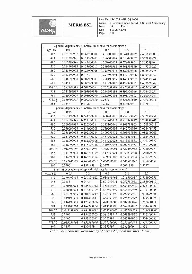
MERIS ESLDoc.No : PO-TN-MEL-GS-0026Name : Referencemodel forMERISLevel 2 processingIssue : 4 Rev.: IDate : 13July 200IPage : 71
Spectral dependency of optical thickness for assemblage 8'ta(560) 0.03 0.1 0.3 0.5 2.0
412 0.077699997 0.162200004 0.403600005 0.644800019 2.45509998443 0.07329999 0.154599903 0.386500009 0.618499867 2.357899874490 0.067299996 0.143400004 0.360900014 0.578499961 2.20979996510 0.064699998 0.138600011 0.349999986 0.561599899 2.147300027560 0.058899995 0.127900006 0.325300012 0.522699906 2.002599978620 0.052799998 0.1163 0.297699994 0.479199906 1.839900057665 0.048599998 0.107999901 0.278199999 0.448399982 1.724599864681 0.0471 0.105399899 0.271899895 0.438399913 1.687000048
708.75 0.045199999 0.101700001 0.262699998 0.423999907 1.632400007753 0.041299997 0.093999999 0.244599894 0.395300016 1.524400054761 0.040999999 0.093099999 0.242399895 0.391399895 1.510099944
778.75 0.039799999 0.090899999 0.2371 0.383399989 1.479599913865 0.0342 0.0796 0.2087 0.3380999 1.3076
Spectral dependency of optical thickness for assemblage 9'ttrooo(560) 0.05 0.2 0.5 0.8 2.0
412 0.067199993 0.244299912 0.600700046 0.957199872 2.382999751443 0.064599995 0.23410001 0.575900012 0.917999917 2.284899907490 0.060599999 0.22030001 0.542100041 0.863799963 2.150800019510 0.059099994 0.214900008 0.529000002 0.842700016 2.098499953560 0.055199995 0.202800014 0.499099912 0.795999956 1.982599963620 0.051299996 0.189700013 0.467900024 0.745699951 1.85849994665 0.048999995 0.181299906 0.447700025 0.713899888 1.779199879681 0.048099997 0.178399918 0.440699993 0.702799983 1.751799966
708.75 0.046899997 0.174500015 0.430799994 0.687399913 1.71309997753 0.044699998 0.166700009 0.412299921 0.657899928 1.640099871761 0.044399997 0.165700004 0.409899883 0.653899984 1.630299972
778.75 0.043900002 0.163699902 0.404800005 0.645900017 1.610800052865 0.0406 0.1521999 0.3771 0.6021999 1.5017
Spectral dependency of optical thickness for assemblage 10't1r0n0(560) 0.05 0.2 0.5 0.8 2.0
412 0.069499998 0.257899922 0.634699995 1.011500017 2.518900051443 0.0658 0.2443 0.601099911 0.957799933 2.385000119490 0.060800001 0.225499912 0.55519999 0.884599943 2.203100059510 0.058600001 0.218299909 0.537499897 0.856699969 2.133100045560 0.054099999 0.201700017 0.497399898 0.792999921 1.974899996620 0.049499999 0.18440001 0.454999995 0.725399977 1.807500078665 0.046199997 0.173500006 0.428000003 0.682500026 1.700600118681 0.045200002 0.169799904 0.41909989 0.668099887 1.664600008
708.75 0.043699999 0.164399911 0.405799885 0.64 7199909 1.612499949753 0.0409 0.154200003 0.381099917 0.608299922 1.516199934761 0.0405 0.153200012 0.378199914 0.603299972 1.503400065
778.75 0.039599998 0.150399996 0.371500005 0.592499898 1.477100077865 0.0357 0.1354999 0.3355999 0.5356999 1.336Table 14-1: Spectral dependency of aerosol optical thickness (cont.)
Copyright © 200 I ACRI SA

MERIS ESLDoc. No : PO-TN-MEL-GS-0026Name : Reference model for MERIS Level 2 processingIssue : 4 Rev.: 1Date : 13 July 2001Page : 72
Spectral dependency of optical thickness for assemblage 11'ttrono(560) 0.05 0.2 0.5 0.8 2.0
412 0.074199998 0.27149998 0.668699931 1.065899915 2.654800083443 0.0696 0.254200009 0.625899926 0.997799899 2.485100171490 0.063 0.230699996 0.568099989 0.905699939 2.255599991510 0.060499998 0.221499988 0.545999898 0.870299855 2.167500137560 0.054799998 0.201100011 0.49529991 0.789799973 1.967000127620 0.048899998 0.179499893 0.442299997 0.705100024 1.756300046665 0.0452 0.165600005 0.408299901 0.651199885 1.621799969681 0.0438 0.160999994 0.397099911 0.633099923 1.577500096
708.75 0.042099999 0.154400006 0.380599887 0.606899931 1.512100056753 0.038400001 0.142000009 0.35009991 0.558500014 1.391700047761 0.037999998 0.14049999 0.346399991 0.55239988 1.376500074
778.75 0.037200001 0.136999994 0.338099913 0.539099894 1.343600049865 0.0322 0.1189 0.2943 0.4693999 1.17
Spectral dependency of optical thickness for assemblage 12'ttrono(560) 0.05 0.2 0.5 0.8 2.0
412 0.065500001 0.237099885 0.582400035 0.927999861 2.309799984443 0.063199998 0.228699992 0.562399934 0.896399869 2.230799943490 0.0599 0.217700005 0.535399911 0.852799855 2.123599977510 0.058500001 0.213199995 0.524499993 0.835499953 2.080700017560 0.055199999 0.202999995 0.499699885 0.796899904 1.984800049620 0.052200003 0.193099991 0.476199873 0.759099859 1.891999884665 0.050100002 0.185900004 0.4591999 0.732299879 1.825300008681 0.049499999 0.18419999 0.455099887 0.725799923 1.809400054
708.75 0.0485 0.180800004 0.446699984 0.712399855 1.776000077753 0.046700001 0.175099896 0.433099986 0.691 1.723000053761 0.046500003 0.174299986 0.431399999 0.688199842 1.716099903
778.75 0.046100003 0.172199902 0.425999986 0.679600013 1.695099975865 0.0433 0.1632 0.4045999 0.6459 1.6113
Spectral dependency of optical thickness for assemblage 13'trrono(560) 0.05 0.2 0.5 0.8 2.0
412 0.068199997 0.253099999 0.622600016 0.992099986 2.47000003 7443 0.064999996 0.2407999 0.591999895 0.943299984 2.348699946490 0.060299997 0.223699887 0.550599981 0.877399938 2.184899948510 0.058400001 0.216999991 0.534500012 0.851899936 2.121200058560 0.054099999 0.201900003 0.497900014 0.793499993 1.976400031620 0.049899995 0.186700004 0.460599906 0.73429975 1.829699967665 0.046999995 0.1765999 0.435600006 0.694899949 1.731199891681 0.0462 0.173699898 0.428699921 0.683399972 1.70309988
708.75 0.044799998 0.168500009 0.416299895 0.663799874 1.654499947753 0.042199999 0.159799902 0.395099925 0.630399955 1.571400001761 0.041899998 0.158899993 0.392599898 0.626099968 1.560799841
778.75 0.041099999 0.156000008 0.385699898 0.615000008 1.533499846865 0.0375 0.1428 0.3538999 0.5651 1.409
Table 14-1: Spectral dependency of aerosol optical thickness (cont.)
Copyright© 2001ACRI S.A.
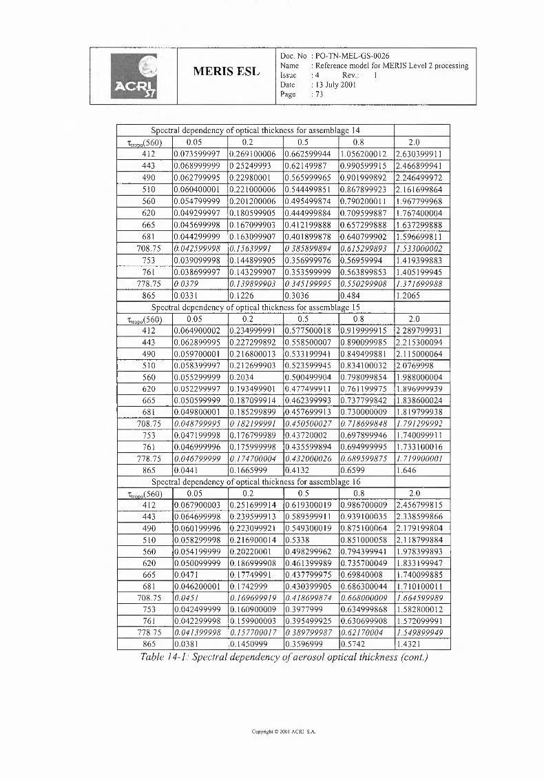
MERIS ESLDoc.No : PO-TN-MEL-GS-0026Name : Referencemodel forMERISLevel 2 processingIssue : 4 Rev.: 1Date : 13July 2001Page : 73
Spectral dependency of optical thickness for assemblage 14'ttrooo(560) 0.05 0.2 0.5 0.8 2.0
412 0.073599997 0.269100006 0.662599944 1.056200012 2.630399911443 0.068999999 0.25249993 0.62149987 0.990599915 2.466899941490 0.062799995 0.22980001 0.565999965 0.901999892 2.246499972510 0.060400001 0.221000006 0.544499851 0.867899923 2.161699864560 0.054799999 0.201200006 0.495499874 0.790200011 1.967799968620 0.049299997 0.180599905 0.444999884 0.709599887 1.767400004665 0.045699998 0.167099903 0.412199888 0.657299888 1.637299888681 0.044299999 0.163099907 0.401899878 0.640799902 1.596699811
708.75 0.042599998 0.15639991 0.385899894 0.615299893 1.533000002753 0.039099998 0.144899905 0.356999976 0.56959994 1.419399883761 0.038699997 0.143299907 0.353599999 0.563899853 1.405199945
778.75 0.0379 0.139899903 0.345199995 0.550299908 1.371699988865 0.0331 0.1226 0.3036 0.484 1.2065
Spectral dependency of optical thickness for assemblage 15'ttrooo(560) 0.05 0.2 0.5 0.8 2.0
412 0.064900002 0.234999991 0.577500018 0.919999915 2.289799931443 0.062899995 0.227299892 0.558500007 0.890099985 2.215300094490 0.059700001 0.216800013 0.533199941 0.849499881 2.115000064510 0.058399997 0.212699903 0.523599945 0.834100032 2.0769998560 0.055299999 0.2034 0.500499904 0.798099854 1.988000004620 0.052299997 0.193499901 0.477499911 0.761199975 1.896999939665 0.050599999 0.187099914 0.462399993 0.737799842 1.838600024681 0.049800001 0.185299899 0.457699913 0.730000009 1.819799938
708.75 0.048799995 0.182199991 0.450500027 0.718699848 1.791299992753 0.047199998 0.176799989 0.43720002 0.697899946 1.740099911761 0.046999996 0.175999998 0.435599894 0.694999995 1.733100016
778.75 0.046799999 0.174700004 0.432000026 0.689599875 1.719900001865 0.0441 0.1665999 0.4132 0.6599 1.646
Spectral dependency of optical thickness for assemblage 16'ttrooo(560) 0.05 0.2 0.5 0.8 2.0
412 0.067900003 0.251699914 0.619300019 0.986700009 2.456799815443 0.064699998 0.239599913 0.589599911 0.939100035 2.338599866490 0.060199996 0.223099921 0.549300019 0.875100064 2.179199804510 0.058299998 0.216900014 0.5338 0.851000058 2.118799884560 0.054199999 0.20220001 0.498299962 0.794399941 1.978399893620 0.050099999 0.186999908 0.461399989 0.735700049 1.833199947665 0.0471 0.17749991 0.437799975 0.69840008 1.740099885681 0.046200001 0.1742999 0.430399905 0.686300044 1.710 100011
708.75 0.0451 0.169699919 0.418699874 0.668000009 1.664599989753 0.042499999 0.160900009 0.3977999 0.634999868 1.582800012761 0.042299998 0.159900003 0.395499925 0.630699908 1.572099991
778.75 0.0413 99998 0.157700017 0.389799987 0.62170004 1.549899949865 0.0381 0.1450999 0.3596999 0.5742 1.4321Table 14-1: Spectral dependency of aerosol optical thickness (cont.)
Copyright ID200 I ACRI SA
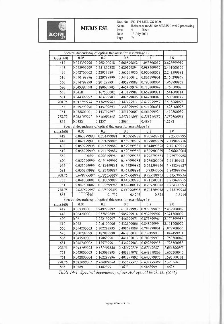
MERIS ESLDoc.No : PO-TN-MEL-GS-0026Name : Referencemodel forMERISLevel2 processingIssue : 4 Rev.: IDate : 13July 200IPage : 74
Spectral dependency of optical thickness for assemblage 17'ttrono(560) 0.05 0.2 0.5 0.8 2.0
412 0.073399996 0.268400018 0.660899852 1.053600017 2.623699919443 0.068999999 0.251899888 0.620199894 0.988599957 2.461900179490 0.062700002 0.22959989 0.565299936 0.900900053 2.243599981510 0.060199996 0.220799999 0.544200012 0.867599901 2.160399967560 0.054799999 0.201299991 0.495899888 0.790500004 1.968899962620 0.049399998 0.180699905 0.445499974 0.710300042 1.76910002665 0.0458 0.167500002 0.413199982 0.659200021 1.641600114681 0.044399997 0.163299903 0.402699896 0.64230004 1.600200147
708.75 0.042799998 0.156999903 0.387199911 0.617299957 1.538000073753 0.039299996 0.145299893 0.358399996 0.571900031 1.425100075761 0.038800001 0.143799897 0.355100007 0.566099924 1.410800039
778.75 0.038100001 0.140699893 0.347199893 0.553599885 1.380100083865 0.0333 0.1237 0.3064 0.4886 1.2182
Spectral dependency of optical thickness for assemblage 18'ttrooo(560) 0.05 0.2 0.5 0.8 2.0
412 0.063899998 0.231499891 0.56859988 0.905699913 2.25389995443 0.062199997 0.224599896 0.552199909 0.879899959 2.189899776490 0.059299998 0.215399889 0.529799881 0.844099898 2.101699913510 0.058299999 0.211699887 0.520799856 0.829900029 2.06640004560 0.0554 0.203499984 0.500999938 0.798799884 1.989799968620 0.052799999 0.194899992 0.480999983 0.766800006 1.911099921665 0.051099999 0.189199881 0.467299882 0.745599976 1.858299927681 0.050299998 0.187499884 0.463599884 0.73940006 1.842999996
708.75 0.049499997 0.185099889 0.457399998 0.729799953 1.819199918753 0.048000001 0.180099897 0.445699996 0.711300011 1.773699955761 0.047800002 0.179599988 0.444400019 0.709200048 1.768300093
778.75 0.047699997 0.178099892 0.440900008 0.703700058 1.755199946865 0.0454 0.1712 0.4246 0.678 1.6914
Spectral dependency of optical thickness for assemblage 19'ttr000(560) 0.05 0.2 0.5 0.8 2.0
412 0.067300001 0.249299892 0.613199993 0.977099875 2.432900062443 0.064200001 0.237899889 0.585299914 0.932399907 2.321500092490 0.06 0.222199997 0.546999971 0.871699964 2.170399988510 0.058 0.216100006 0.532100006 0.84809999 2.111700079560 0.054200003 0.202299993 0.498699889 0.794999901 1.979700006620 0.050299999 0.187899998 0.463800031 0.73949993 1.842499971665 0.047500001 0.178699901 0.441100013 0.70369997 1.753300049681 0.046700002 0.175799901 0.434299983 0.692399938 1.725500088
708.75 0.045400003 0.171499886 0.423499919 0.67549987 1.683300045753 0.043000003 0.163099893 0.403399978 0.643999869 1.605200045761 0.042800004 0.162299896 0.401299892 0.640099975 1.595500101
778.75 0.042000001 0.160099884 0.395599973 0.631199897 1.5736001865 0.0389 0.1482999 0.3673 0.5863999 1.4625Table 14-1: Spectral dependency of aerosol optical thickness (cont.)
Copyright© 2001ACRI S.A.
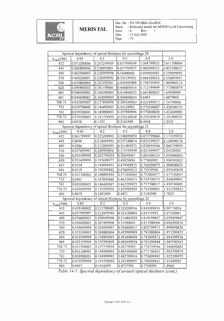
MERIS ESLDoc.No : PO-TN-MEL-GS-0026Name : Referencemodel for MERISLevel 2 processingIssue : 4 Rev.: 1Date : 13July 2001Page : 75
Spectral dependency of optical thickness for assemblage 20'ttrono(560) 0.05 0.2 0.5 0.8 2.0
412 0.073200006 0.267299989 0.657999899 1.048799935 2.611700064443 0.068800006 0.250999891 0.617999957 0.985099933 2.453300037490 0.062500003 0.228999998 0.56400002 0.899099982 2.239099992510 0.060200001 0.220499992 0.543199901 0.866100018 2.156899961560 0.054800004 0.201299981 0.495999909 0.790799959 1.969400114620 0.049400003 0.181199885 0.446600014 0.712199999 1.773800079665 0.046000001 0.168099889 0.414800023 0.661800002 1.64820009681 0.044600001 0.164099899 0.404800019 0.6454 1.6079001
708.75 0.043000005 0.157899896 0.389399903 0.621099872 1.54740006753 0.039700002 0.146499902 0.36129993 0.576300007 1.436300135761 0.039200001 0.145099893 0.357899996 0.570800028 1.422600085
778.75 0.038500003 0.141799999 0.350100038 0.558399959 1.391800101865 0.0338 0.1253 0.3101999 0.4948 1.2332
Spectral dependency of optical thickness for assemblage 21'ttrooo(560) 0.05 0.2 0.5 0.8 2.0
412 0.061799997 0.223299892 0.548099859 0.872799868 2.172399932443 0.0604 0.218699992 0.537100014 0.855399937 2.128900138490 0.0586 0.212099995 0.521499872 0.830999944 2.068799895510 0.057699997 0.209499896 0.515599999 0.821499997 2.04530002560 0.055599998 0.203799994 0.50249987 0.801000135 1.995000003620 0.053499999 0.197699977 0.48829988 0.77869992 1.940300022665 0.0524 0.194099893 0.479499875 0.764500079 1.906000032681 0.0519 0.192599882 0.476099912 0.75959996 1.893600054
708.75 0.051300002 0.190899986 0.4 71800004 0.753000077 1.877100091753 0.0501 0.187099888 0.463299913 0.739700072 1.844699981761 0.050000003 0.186499887 0.462299925 0.737700017 1.839700005
778.75 0.049499996 0.185899996 0.459999989 0.734300045 1.831599933865 0.0478 0.1801999 0.4471 0.7143999 1.7823
Spectral dependency of optical thickness for assemblage 22'ttrooo(560) 0.05 0.2 0.5 0.8 2.0
412 0.059100002 0.215700003 0.529299916 0.843099919 2.09770016443 0.057999997 0.212899988 0.523100048 0.83319992 2.07320001490 0.056600003 0.209099908 0.514400028 0.819199867 2.039499887510 0.056000002 0.207499896 0.51090002 0.813900066 2.026500016560 0.054699998 0.204299987 0.503600017 0.802799973 1.999699826620 0.053500003 0.200800004 0.495999909 0.791000004 1.971299855665 0.052599999 0.198899985 0.491600044 0.783899872 1.954399936681 0.052199999 0.197999899 0.489699928 0.781299844 1.947999943
708.75 0.051900002 0.197199994 0.48779993 0.778199946 1.940099885753 0.051100001 0.194999903 0.483500008 0.771700051 1.92479997 4761 0.050900001 0.194999993 0.482799916 0.770899983 1.922399972
778.75 0.050599998 0.194599984 0.481899997 0.769099841 1.91889992865 0.0497 0.1916999 0.4757999 0.7598999 1.8968Table 14-1: Spectral dependency of aerosol optical thickness (cont.)
Copyright© 200I ACRI S.A.
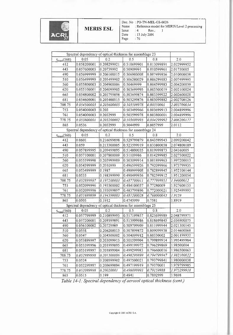
Doc. No : PO-TN-MEL-GS-0026Name : Reference model for MERIS Level 2 processingIssue : 4 Rev.: IDate : 13July 200 IPage : 76
MERIS ESL
Spectral dependency of optical thickness for assemblage 23'ttrono(560) 0.05 0.2 0.5 0.8 2.0
412 0.058200001 0.208299921 0.510699901 0.813099891 2.022999952443 0.057600003 0.20739992 0.50909991 0.810599961 2.01730005490 0.056999999 0.206100015 0.506900008 0.807499856 2.010000038510 0.056499999 0.205499902 0.506200029 0.806299883 2.007499995560 0.055800003 0.204900006 0.50469999 0.804599983 2.004200039620 0.055100001 0.204099905 0.503699995 0.803300019 2.002100024665 0.054800002 0.203799898 0.503699874 0.803399922 2.002600028681 0.054600001 0.203400015 0.503299876 0.803099882 2.002700126
708.75 0.054500003 0.203600005 0.503599978 0.80350001 2.003700034753 0.054000003 0.203 0.503499966 0.803699913 2.004899996761 0.054000003 0.2032999 0.503599978 0.803800001 2.004899996
778.75 0.053800001 0.203200002 0.503699995 0.804299992 2.006200177865 0.0536 0.2032999 0.5044999 0.8057999 2.0112
Spectral dependency of optical thickness for assemblage 24'ttrooo(560) 0.05 0.2 0.5 0.8 2.0
412 0.0601 0.216099898 0.529799879 0.843599943 2.099200042443 0.059 0.213300005 0.523599919 0.833800038 2.074800189490 0.057899995 0.209499895 0.514800035 0.819999873 2.04160005510 0.057100001 0.207800009 0.51109986 0.814299985 2.027500022560 0.055599998 0.203999989 0.503099914 0.801899963 1.997200013620 0.054399999 0.2010999 0.496599926 0.792099966 1.973799935665 0.053499999 0.1987 0.490999908 0.782899945 1.952100144681 0.0533 0.198399999 0.490499936 0.782599912 1.951200054
708.75 0.052899997 0.197200003 0.487700011 0.7779999 51 1.94000012753 0.052099996 0.195500002 0.484100037 0.77280009 1.927600153761 0.052099996 0.195099897 0.483 799896 0.772000021 1.925499993
778.75 0.051699999 0.194399883 0.481200028 0.768000043 1.9159865 0.0505 0.1912 0.4745999 0.7581 1.8919
Spectral dependency of optical thickness for assemblage 25'ttrooo(560) 0.05 0.2 0.5 0.8 2.0
412 0.057799999 0.210899993 0.517199857 0.823699989 2.048799971443 0.057200001 0.209399891 0.513999986 0.818699845 2.036900075490 0.056100002 0.20729989 0.509799909 0.811999944 2.021300145510 0.0558 0.206200013 0.507899872 0.809099938 2.014600068560 0.0547 0.204500002 0.504099912 0.80330002 2.001199932620 0.053899997 0.203099913 0.501599904 0.799899914 1.993499984665 0.053399996 0.201999895 0.499199972 0.796299869 1.98500004681 0.053199997 0.201899904 0.499299983 0.796600016 1.986500063
708.75 0.052999998 0.201300006 0.498299899 0.794799947 1.982100022753 0.0524 0.200599902 0.497500021 0.793799841 1.980000038761 0.052299997 0.200699894 0.497199919 0.79370001 1.979799985
778.75 0.052099998 0.20020001 0.496099993 0.79159988 1.975299918865 0.0515 0.199 0.4941 0.7892999 1.9698Table 14-1: Spectral dependency of aerosol optical thickness (cont.)
Copyright 11:>200 I ACRI S.A.
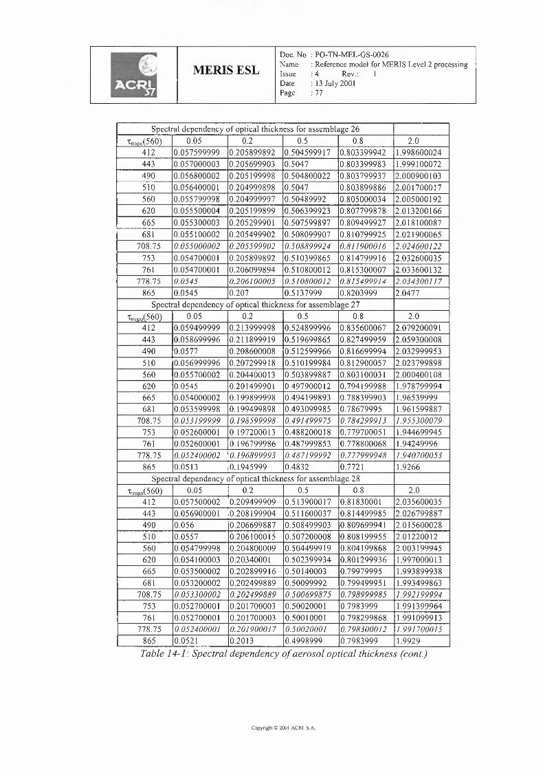
MERIS ESLDoc.No : PO-TN-MEL-GS-0026Name : Referencemodel forMERISLevel 2 processingIssue : 4 Rev.: IDate : 13July 2001Page : 77
Spectral dependency of optical thickness for assemblage 26'ttrono(560) 0.05 0.2 0.5 0.8 2.0
412 0.057599999 0.205899892 0.504599917 0.803399942 1.998600024443 0.057000003 0.205699903 0.5047 0.803399983 1.999100072490 0.056800002 0.205199998 0.504800022 0.803799937 2.000900103510 0.056400001 0.204999898 0.5047 0.803899886 2.001700017560 0.055799998 0.204999997 0.50489992 0.805000034 2.005000192620 0.055500004 0.205199899 0.506399923 0.807799878 2.013200166665 0.055300003 0.205299901 0.507599897 0.809499927 2.018100087681 0.055100002 0.205499902 0.508099907 0.810799925 2.021900065
708.75 0.055000002 0.205599902 0.508899924 0.811900016 2.024600122753 0.054700001 0.205899892 0.510399865 0.814799916 2.032600035761 0.054700001 0.206099894 0.510800012 0.815300007 2.033600132
778.75 0.0545 0.206100005 0.510800012 0.815499914 2.034300117865 0.0545 0.207 0.5137999 0.8203999 2.0477
Spectral dependency of optical thickness for assemblage 27'ttrono(560) 0.05 0.2 0.5 0.8 2.0
412 0.059499999 0.213999998 0.524899996 0.835600067 2.079200091443 0.058699996 0.211899919 0.519699865 0.827499959 2.059300008490 0.0577 0.208600008 0.512599966 0.816699994 2.032999953510 0.056999996 0.207299918 0.510199984 0.812900057 2.023799898560 0.055700002 0.204400013 0.503899887 0.803100031 2.000400108620 0.0545 0.201499901 0.497900012 0.794199988 1.978799994665 0.054000002 0.199899998 0.494199893 0.788399903 1.96539999681 0.053599998 0.199499898 0.493099985 0.78679995 1.961599887
708.75 0.053199999 0.198599998 0.491499975 0.784299913 1.955300079753 0.052600001 0.197200013 0.488200018 0.779700051 1.944699945761 0.052600001 0.196799986 0.487999853 0.778800068 1.94249996
778.75 0.052400002 0.196899993 0.487199992 0.777999948 1.940700053865 0.0513 0.1945999 0.4832 0.7721 1.9266
Spectral dependency of optical thickness for assemblage 28'ttrono(560) 0.05 0.2 0.5 0.8 2.0
412 0.057500002 0.209499909 0.513900017 0.81830001 2.035600035443 0.056900001 0.208199904 0.51160003 7 0.814499985 2.026799887490 0.056 0.206699887 0.508499903 0.809699941 2.015600028510 0.0557 0.206100015 0.507200008 0.808199955 2.01220012560 0.054799998 0.204800009 0.504499919 0.804199868 2.003199945620 0.054100003 0.20340001 0.502399934 0.801299936 1.997000013665 0.053500002 0.202899916 0.50140003 0.79979995 1.993899938681 0.053200002 0.202499889 0.50099992 0.799499951 1.993499863
708.75 0.053300002 0.202499889 0.500699875 0.798999985 1.992199994753 0.052700001 0.201700003 0.50020001 0.7983999 1.991399964761 0.052700001 0.201700003 0.50010001 0.798299868 1.991099913
778.75 0.052400001 0.201900017 0.50020001 0.798300012 1.991700015865 0.0521 0.2013 0.4998999 0.7983999 1.9929Table 14-1: Spectral dependency of aerosol optical thickness (cont.)
Copyright I:>200 I ACRI SA
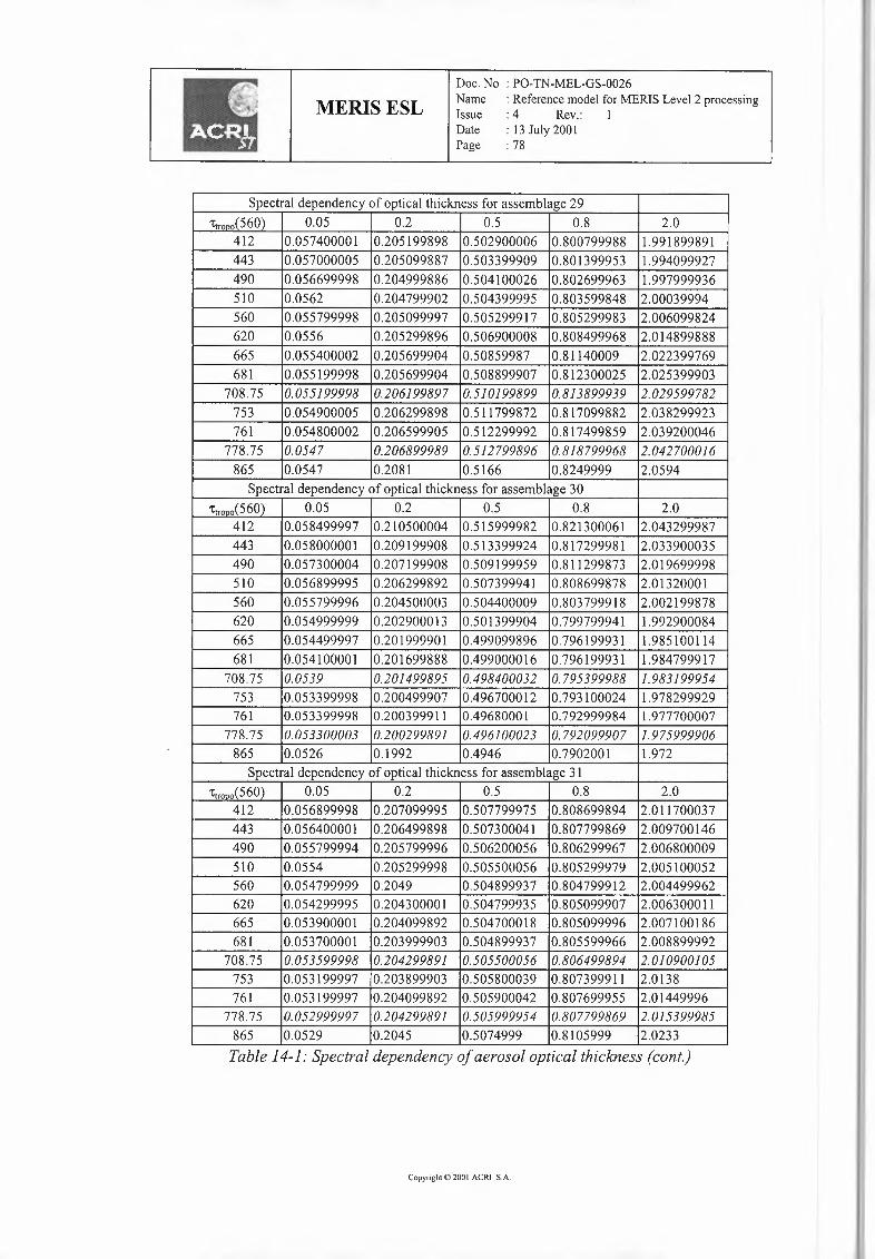
MERIS ESLDoc. No : PO-TN-MEL-GS-0026Name : Reference model for MERIS Level 2 processingIssue : 4 Rev.: 1Date : 13 July 2001Page : 78
Spectral dependency of optical thickness for assemblage 29'tn-000(560) 0.05 0.2 0.5 0.8 2.0
412 0.057400001 0.205199898 0.502900006 0.800799988 1.991899891443 0.057000005 0.205099887 0.503399909 0.801399953 1.994099927490 0.056699998 0.204999886 0.504100026 0.802699963 1.997999936510 0.0562 0.204799902 0.504399995 0.803599848 2.00039994560 0.055799998 0.205099997 0.505299917 0.805299983 2.006099824620 0.0556 0.205299896 0.506900008 0.808499968 2.014899888665 0.055400002 0.205699904 0.50859987 0.81140009 2.022399769681 0.055199998 0.205699904 0.508899907 0.812300025 2.025399903
708.75 0.055199998 0.206199897 0.510199899 0.813899939 2.029599782753 0.054900005 0.206299898 0.511799872 0.817099882 2.038299923761 0.054800002 0.206599905 0.512299992 0.817499859 2.039200046
778.75 0.0547 0.206899989 0.512 799896 0.818 799968 2.042700016865 0.0547 0.2081 0.5166 0.8249999 2.0594
Spectral dependency of optical thickness for assemblage 30'ttrooo(560) 0.05 0.2 0.5 0.8 2.0
412 0.058499997 0.210500004 0.515999982 0.821300061 2.043299987443 0.058000001 0.209199908 0.513399924 0.817299981 2.033900035490 0.057300004 0.207199908 0.509199959 0.811299873 2.019699998510 0.056899995 0.206299892 0.507399941 0.808699878 2.01320001560 0.055799996 0.204500003 0.504400009 0.803 799918 2.002199878620 0.054999999 0.202900013 0.501399904 0.799799941 1.992900084665 0.054499997 0.201999901 0.499099896 0.796199931 1.985100114681 0.054100001 0.201699888 0.499000016 0.796199931 1.984799917
708.75 0.0539 0.201499895 0.498400032 0.795399988 1.983199954753 0.053399998 0.200499907 0.496700012 0.793100024 1.978299929761 0.053399998 0.200399911 0.49680001 0.792999984 1.977700007
778.75 0.053300003 0.200299891 0.496100023 0.792099907 1.975999906865 0.0526 0.1992 0.4946 0.7902001 1.972
Spectral dependency of optical thickness for assemblage 31'ttrono(560) 0.05 0.2 0.5 0.8 2.0
412 0.056899998 0.207099995 0.507799975 0.808699894 2.011700037443 0.056400001 0.206499898 0.507300041 0.807799869 2.009700146490 0.055799994 0.205799996 0.506200056 0.806299967 2.006800009510 0.0554 0.205299998 0.505500056 0.805299979 2.005100052560 0.054799999 0.2049 0.504899937 0.804799912 2.004499962620 0.054299995 0.204300001 0.504799935 0.805099907 2.006300011665 0.053900001 0.204099892 0.504700018 0.805099996 2.007100186681 0.053700001 0.203999903 0.504899937 0.805599966 2.008899992
708.75 0.053599998 0.204299891 0.505500056 0.806499894 2.010900105753 0.053199997 0.203899903 0.505800039 0.807399911 2.0138761 0.053199997 0.204099892 0.505900042 0.807699955 2.01449996
778.75 0.052999997 0.204299891 0.505999954 0.807799869 2.015399985865 0.0529 0.2045 0.5074999 0.8105999 2.0233Table 14-1: Spectral dependency of aerosol optical thickness (cont.)
Copyright© 2001ACRI S.A.
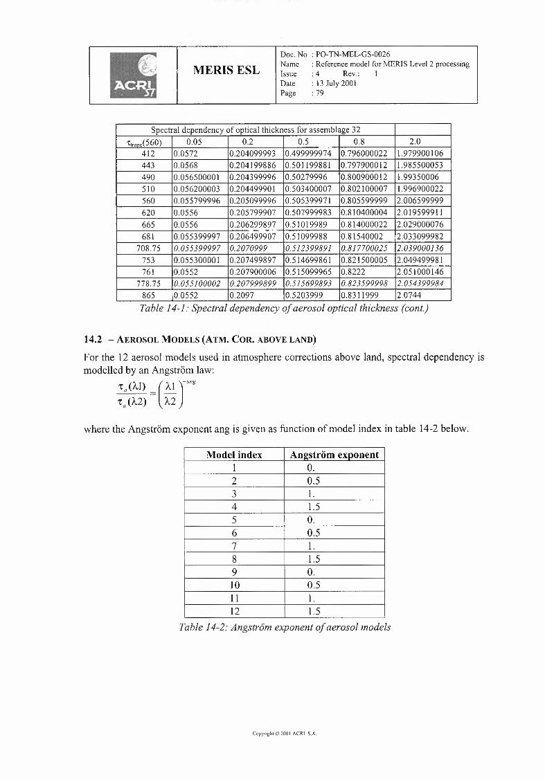
MERIS ESLDoc. No : PO-TN-MEL-GS-0026Name : Reference model for MERIS Level 2 processingIssue : 4 Rev.: IDate : 13July 2001Page : 79
Spectral dependency of optical thickness for assemblage 32'ttrono(560) 0.05 0.2 0.5 0.8 2.0
412 0.0572 0.204099993 0.499999974 0.796000022 1.979900106443 0.0568 0.204199886 0.501199881 0.797900012 1.985500053490 0.056500001 0.204399996 0.50279996 0.800900012 1.99350006510 0.056200003 0.204499901 0.503400007 0.802100007 1.996900022560 0.055799996 0.205099996 0.505399971 0.805599999 2.006599999620 0.0556 0.205799907 0.507999983 0.810400004 2.019599911665 0.0556 0.206299897 0.51019989 0.814000022 2.029000076681 0.055399997 0.206499907 0.51099988 0.81540002 2.033099982
708.75 0.055399997 0.2070999 0.512399891 0.817700025 2.039000136753 0.055300001 0.207499897 0.514699861 0.821500005 2.049499981761 0.0552 0.207900006 0.515099965 0.8222 2.051000146
778.75 0.055100002 0.207999899 0.515699893 0.823599998 2.054399984865 0.0552 0.2097 0.5203999 0.8311999 2.0744Table 14-1: Spectral dependency of aerosol optical thickness (cont.)
14.2 -AEROSOL MODELS (ATM. COR. ABOVE LAND)
For the 12 aerosol models used in atmosphere corrections above land, spectral dependency ismodelled by an Angstrom law:
'ta (Al) = (~ )-ang'ta (A.2) A-2
where the Angstrom exponent ang is given as function of model index in table 14-2 below.
Model index Anzstrorn exponent1 0.2 0.53 1.4 1.55 0.6 0.57 1.8 1.59 0.10 0.511 1.12 1.5
Table 14-2: Angstrom exponent of aerosol models
Copyright © 200 I ACRI S.A.
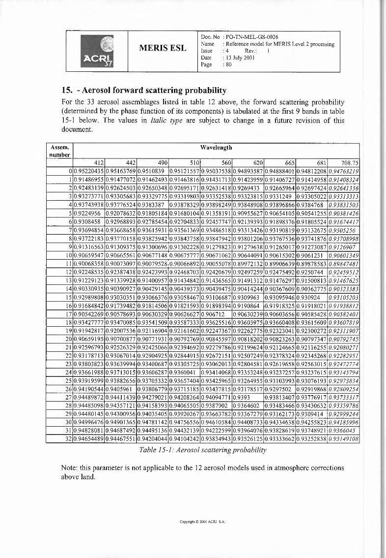
MERIS ESLDoc.No : PO-TN-MEL-GS-0026Name : Referencemodel forMERISLevel 2 processingIssue : 4 Rev.: 1Date : 13July 2001Page : 80
15. -Aerosol forward scattering probabilityFor the 33 aerosol assemblages listed in table 12 above, the forward scattering probability(determined by the phase function of its components) is tabulated at the first 9 bands in table15-1 below. The values in Italic type are subject to change in a future revision of thisdocument.
Assem. Wavelengthnumber
412 442 490 510 560 620 665 681 708.750 0.95220435 0.95163769 0.9510839 0.95121557 0.95037538 0.94893587 0.94888401 0.94812208 0.947632191 0.91486955 0.91477072 0.91462493 0.91463816 0.91431713 0.91423959 0.91406727 0.91414958 0.914083242 0.92483139 0.92624503 0.92650348 0.92695171 0.92631418 0.9269433 0.92665964 0.92697424 0.926413363 0.93273771 0.93305683 0.93329775 0.93319803 0.93352538 0.93323815 0.9331249 0.93305022 0.933133134 0.93743938 0.93776524 0.9383387 0.93878329 0.93898249 0.93848908 0.93896866 0.9384768 0.938315035 0.9224956 0.92078632 0.91805184 0.91680104 0.91358191 0.90955627 0.90654105 0.90541255 0.903814266 0.9308458 0.92968893 0.92785454 0.92704833 0.92457747 0.92139393 0.91898376 0.91805524 0.916744177 0.93694854 0.93668658 0.93615931 0.93561369 0.93486518 0.93313426 0.93190819 0.93132675 0.93052568 0.93722183 0.93770158 0.93825942 0.93843758 0.93847942 0.93801206 0.93767536 0.93741876 0.937089989 0.91316563 0.91309375 0.91300696 0.91302228 0.91279823 0.91279638 0.91265017 0.91273087 0.912690710 0.90659547 0.90665561 0.90677148 0.90675777 0.90671062 0.90644091 0.90615302 0.9061231 0.9060134911 0.90068358 0.90073097 0.90079528 0.90066892 0.90055078 0.89972132 0.89906639 0.89878583 0.8984748112 0.92248535 0.92387438 0.92423993 0.92468703 0.92420679 0.92497259 0.92475492 0.9250744 0.9245951213 0.91229123 0.91339928 0.91400957 0.91434842 0.91436565 0.91491312 0.91476297 0.91500813 0.9146762514 0.90330935 0.90390927 0.90429145 0.90439373 0.90439475 0.90414244 0.90367609 0.90362775 0.9032338315 0.92989808 0.93030351 0.93066376 0.93058467 0.93106687 0.9309963 0.93095946 0.930924 0.9310520316 0.91684842 0.91739482 0.91814506 0.91821593 0.91898394 0.9190864 0.91918325 0.91918021 0.9193881217 0.90542269 0.90578693 0.90630329 0.90626627 0.906712 0.90630239 0.90603656 0.90585428 0.9058240118 0.93427777 0.93470085 0.93541509 0.93587333 0.93625516 0.93603975 0.93660408 0.93615609 0.9360781919 0.91942817 0.92007536 0.92116904 0.92161602 0.92247367 0.92262775 0.92323041 0.92300272 0.9231190720 0.90659195 0.90700877 0.90771931 0.90792769 0.90845597 0.90818202 0.90823263 0.90797347 0.9079274521 0.92596793 0.92526329 0.92425066 0.92394692 0.92279786 0.92199624 0.92124665 0.92116255 0.9208027122 0.93178713 0.93067014 0.92904925 0.92844915 0.92672151 0.92507249 0.92378324 0.92345268 0.9228295123 0.93803823 0.93639994 0.93400687 0.93305725 0.93062013 0.92804581 0.92619658 0.92563015 0.9247277424 0.93661988 0.93713015 0.93606287 0.9360041 0.93414068 0.93353248 0.93237257 0.93237615 0.9314579425 0.93919599 0.93882656 0.93705332 0.93657404 0.93425965 0.93264955 0.93103993 0.93076193 0.9297383426 0.94190544 0.9405961 0.93806779 0.93715185 0.93437815 0.93178517 0.9297502 0.92919868 0.9280925427 0.94489872 0.94411439 0.94279021 0.94208264 0.94094771 0.9393 0.93813407 0.93776917 0.9373331728 0.94485098 0.94357121 0.94158393 0.94065505 0.9387902 0.9364602 0.93483466 0.93430632 0.9335978629 0.94480145 0.94300956 0.94035405 0.93920267 0.93663782 0.93367279 0.93162173 0.9309414 0.9299924430 0.94996476 0.94901365 0.94781142 0.94756556 0.94610584 0.94408733 0.94334638 0.94255823 0.9418599631 0.94828081 0.94687492 0.94495136 0.94432139 0.94222599 0.93964076 0.93828619 0.93748921 0.936604532 0.94654489 0.94467551 0.94204044 0.94104242 0.93834943 0.93526125 0.93333662 0.93252838 0.93149108
Table 15-1: Aerosol scattering probability
Note: this parameter is not applicable to the 12 aerosol models used in atmosphere correctionsabove land.
Copyright© 2001ACRI S.A.