Title A Method for Calculating Multi-Dimensional...

http://repository.osakafu-u.ac.jp/dspace/

Title A Method for Calculating Multi-Dimensional Gaussian Distribution

Author(s)Murotsu, Yoshisada; Yonezawa, Masaaki; Oba, Fuminori; Niwa, Kazuku

ni

Editor(s)

CitationBulletin of University of Osaka Prefecture. Series A, Engineering and nat

ural sciences. 1976, 24(2), p.193-204

Issue Date 1976-03-31

URL http://hdl.handle.net/10466/8270

Rights

193

A Method for Calculating Multi-Dimensional

Gaussian Distribution

Yoshisada MuRoTsu*, Masaaki YoNEzAwA**, Fuminori OBA*** and

Kazukuni NiwA****

(Received November 15, 1975)

A method for calculating multi-dimensional Gaussian distributions is proposed, using the Herrnite polynomial expansion method. An algorithmiclproce-

dure is developed for calculating probability distribution functions of arbitrary

dimensions taking account of moment terms up to an arbitrary order. Numerical

exarnple$ are provided to demonstrate the applicability of the proposed procedure.

1. Introduction

Multi-dimensional Gaussian distribution has been widely used in science') and

engineering2), and its properties are discussed in many literatures on statistics3)`). For

the calculation of probabi!ity distribution functions (p.d.f), multiple integrals must be

performed by direct numerical integration or by transforming them into sing!e integral

using orthogonal transformation. However, it does not seem to the authors that these

methods may be eMcient fbr a fast numerical calculation of multi-dimensional Gaussian

probability distribution functions.

In this paper, the Hermite polynomial expansion method is applied for calculating

multi-dimensional Gaussian distributions. Through this method, multiple integrals

encountered in the calculation of the p.d.f are reduced to term-by-term integration of one

variable, which saves greatly computational effbrts. An algorithmic procedure is de-

veloped for calculating the p.d.f of arbitrary dimensions taking account of the moment

terms up to an arbitrary order. Numerical examples are presented for demonstrating the

applicability of the proposed method. Are discussed the effects of correlation coef-

ficients, the order of mement terms and the dimensions of the p.d.f on the resulting

values of the p.d.f and the computer processing time.

2. Hermite Polynomial Expansion of Multi-dimensional

Gaussian Distribution

-- The probability denslty function of a k-dimensional Gaussian distribution is written

in the form

* Department of Naval Architecture, College of Engineering.

** Faculty of Science and Technology, Kinki University.

**es Department of Aeronautical Engineering, College of Engineering.

esee** Graduate student, Department of Aeronautical Engineering.

194 Yoshisada MuRoTsu, Masaaki YoNEzAwA, Fuminori OBA and Kazukuni NiwA

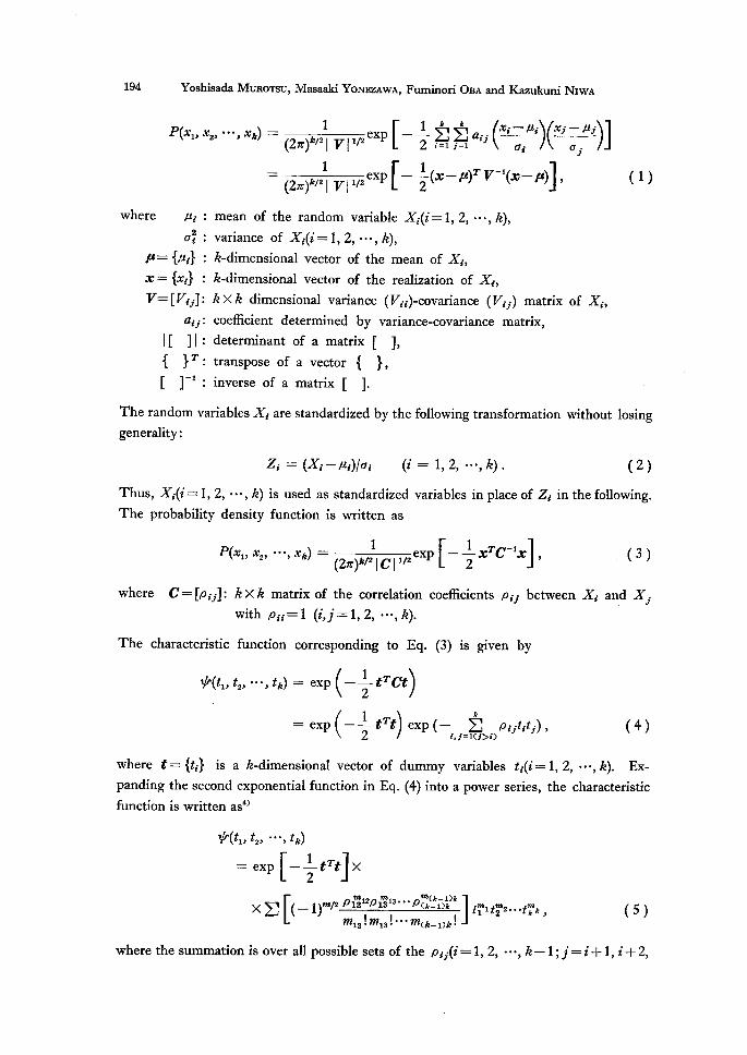
P(xi, x2, "', xk) =: (2va)ky,l vl ,/, exp [--il- te., tS. i, ai7･ (Xi -oipti)(ec" -a7.pti')]

= (2.)kf2il vl ,/, exp [ny -il-(x-iee)Tv-i(co-ize)] , ( 1)

'where pti : mean of the random variable X}(i=1,2, ･･･,k),

o7 : variance of Xi(i=1, 2, ･･･,k),

pt= {pti} : k-dimensional vector of the mean of Xi,

x= {bei} : k-dimensional vector of the realization of X},

V=[V}j]: kXk dimensional variance (V}i)-covariance (Vid) matrix of X},

aii･: coeMcient determined by variance-covariance matrix,

1[ ]1: determinant of a matrix [ ],

{ }T: transpose of a vector { },

[ ]-i:inverse ofa matrix[ ]･

The random variables X) are standardized by the fo11owing transformation without losing

generality:

Zi = (Xi-pti)/ai (i = 1, 2, ･･･, k). (2)

Thus, Xi(i=1, 2, ･･･, k) is used as standardized variables in place of Zi in the fo11owmg.

The probability density function is written as

P(Xi, X2, "', XA) == (2.)k/,IIcl,/, exp [- -i!- xTC-'x] , (3)

where C=[piA: kXk matrix of the correlation coeMcients pi,- between X} and X,-

with pii=1 (i,]'=1, 2, ･･･, k).

The characteristic function corresponding to Eq. (3) is given by

Nee(t,, t,, ･･･, tk) == exp (--ii- tTCt)

tt = exp (--ll- tTt) exp (-,,i.;i(I;j>,)pii･titi･), (4)

where t={ti} is a k-dimensional vector of dummy variables ti(i=1,2, ･･･,k). Ex-

panding the second exponential function in Eq. (4) into a power series, the characteristic

function is written as`)

YO"(t,, t,, "', tk)

= exp [--ll-tTt × ]

xz [(- 1)m12 iilitill, '!2Pmi,M: l3iiijll,2(-ii)i' i/ ] tTi tT2･･･tTk, (5)

where the summation is over all possible sets of the pi,･(i=1, 2, ･･･, k- 1 ij=i+1, i+2,

A Mlethodfor Caleulatiirg Multi-Dimensional Gaussian Distribution

.･･ ,h) taken over all non-negative values of the mii:

i-1 b mi -- Z mji+ Z mii , 1'--1 i=i+1 k m =Zmi･ i--1 ,Let N be defined by

k-1 k N=ZZ mii, i=1 f'=i+1

m in Eq. (6) can be written as

k i-1 h m = Z {2 mj,+ Z mid} i--i+1 i--1 J---1

k i-1 h-1 k = ZZ Mdi+Z Z Mi,･ J'=i+1 i--1 i=2 J' =1

k-1 k =2E] 2] mi,- i=1 i--i+1

== 2N.

where m.(le+,)=m,.==O. Thus it is seen that m is zero or an even number.

defined by Eq. (7), the summation in Eq. (5) can be written in the fbrm:

Nb"(tv t,, ''', tk) = exp [---5--t't]×

×:i ] z (-1)NpiM,i2piM,i3･･･pY,(J",5i,)k tT,tT,...tT,,

N=O CMij')N M12!M13!'''M(k-1)k!

where Z denotes a summation taken over all sets of non-negative values (MisDNwhich satisfy the relation (7) for a given N.

Fourier inversion of sth(t,, t,, ･･･, tk) gives the probability density function:

p(xi) x2, ''', xk) = I:.'''IT..itlT, exp [-it'x] ×

× Nen(t,, t,, ･･･, tk)dt,dt,･･･ dtk

] "" iOO..'"I:..'(2;)leeXP[-it'XellrtTt ×

Xllil, c.1;. Ij)N( - 1)N[ Illti,i!2mP IM,313i i imP Y2(i'i))ihk) i/ ] t?' tT2 ' " tThdtidt2 " ' dtk '

Interchanging summation and integration, Eq. (10) yields

p(x,, x,, ･･･, xk) = NZe=e , (.]I.l]j)pt( - 1)N[ iillM2,i!2mPiM,31/3iiijlli2r(iii))ikk)i/ ] ×

×iliI℃eo in tT' i eXP [-itdXi' - -il7t,'2] dt,･ .

The integral in Eq. (11) is rewritten as

195

(6)

(7)

(8)

Using N

(9)

of the mii

(10)

(11)


21. !:..t7' i exp [-it,･x,･ - -ll- tj2] dti

= ( -2 .i)Mij : .. ( iill . )MjeXP [ - it ,' X,' - Li!- t,' 2] dtj

' = ( re i)Mi( ddx .)Mj iz j:..eXP[-iti'XJ' -}ti2] dtj

J

=(-i)mj( tik .) Mi¢(xv), (i2) '

where ¢(x,･) == v12. 6xp(--S-x,･2). (13) 'The derivatives of ¢(x,･) are related to Hermite polynomials by

(£ )"¢(x) == (-1)"Hh(x)¢(x). (14)

using Eqs. (6), (8), (11), (12) and (14), the probability density function P(x,, x,, ･･･, xk)

is expressed as

p(x,,x,,･･･,xk)=1?"le]m,,th..,.[ t,2,'!2mPIM,313ii'illi-i'kk)l/]te.,H.j(x,･)¢(x,.). (ls)

Using Eqs. (14) and (15), the probability distribution function is given by

co P(x,, x,, ･･･, xk) == ZA4., (16) "=o

AP2N ==,.l,ili,. £IIMil2£l,3/l3iiimP,:k'(:kl"')lii/ te.,(- i)Hmj-i(xi)¢(x,･), (i7)

where (- 1)H- ,(x,)¢(x,･)- ¢(x,･) =: jX!L¢(t)dt. (18)

The above relations are easily programmed for digital computers, and a general com-

putational algorithm is given in the fo11owing section.

3. AlgorithmicProcedure

Using the relations (7), (16), (17) and (18), an algorithmic procedure can be developed

for calculating the multi--dimensional Gaussian probability distribution functions taking

account of the moment terms to any order. The procedure consists of the fo11owing

steps.

Step 1. Specify the dimension (k), the order of the moment terms retained (NMT)

and the value of xi to calculate the p.d.f.

hStep2. Set P6=1[¢(xi) andN=O. i--1Step 3. Set N=N+1 and perform the summation

Step 4.

The

A Mbthodfor thlculating Multi-Dimensional Gaussian Distribution 197

P ==,.]i.llj,. ff,Mii!2£iM,3i!3ii';iiTi'ilikk'I te.,(-1)llmj-i(x,-)¢(x,-)

fbr all possible sets of non-negative values of the mi,･ which satisfy Eq. (7) fbr

the given N. Putting P,N=P,N.,+P, go to Step 4.

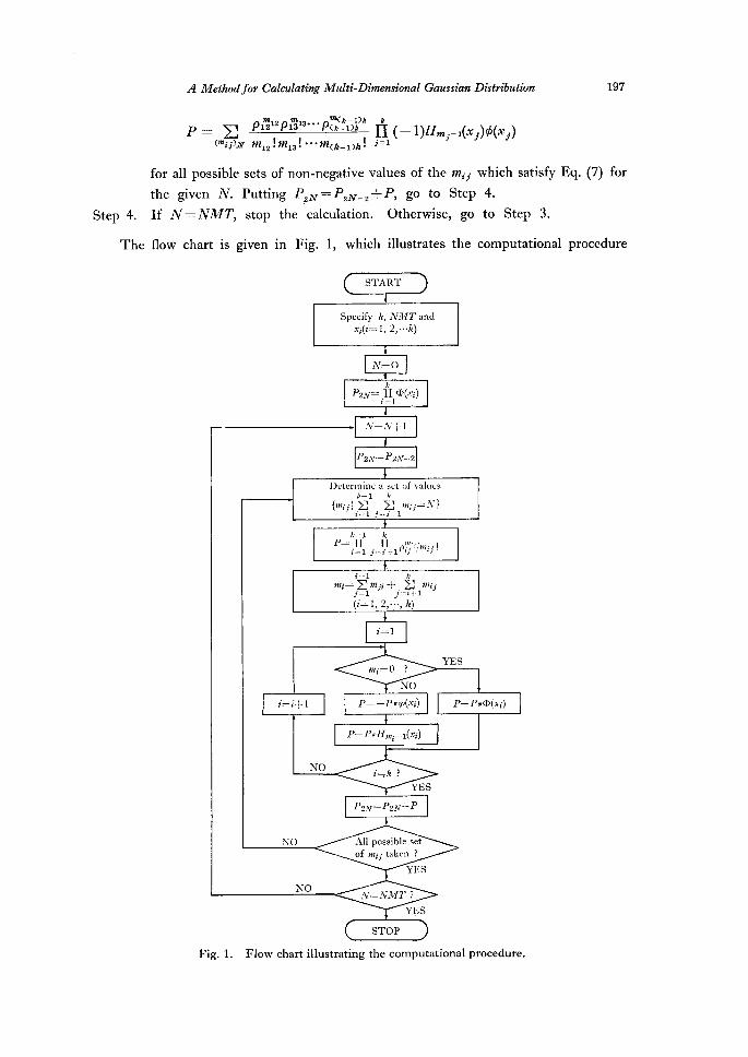
If N=NMT, stop the calculation. Otherwise, go to Step 3.

fiow chart is given in Fig. 1, which illustrates the computational procedure

START

g.pecifyk,N2WrTandxi(i･-=1,2,･･･k)

N=OkP2N=IIO(xi)i,-1

N'±=ATi-･1

P21v=-=-P2N-2

I)etorinineasetofvalLies

k-1k

le--1k.P= il.I..ii,,.I,II÷ipl}{'if,nii!

i--1h2iti=ZMji+,Znli]'y=-i-[-1i-1(i--1,2,･r･,]e)

i=1

mi-=O?

NO

YES

ir-i-l-1 P=-P*ip(xi) P=.=P*tp(xi)

P=--P*Hm･-1(xi)t

'

NO iik?YES

P2N=-P2N+P

NO

NO

Allpossibleset

ofmiitaken?

YES

N=.;rNilf7'?

YES

STOP'

Fig. 1. Flow chart illustrating the computational procedure.


mentioned above.

4. NumericalExamples

First consider a two dimensional case. The values of the probability distribution

function

P(X" sc2) = jX"'coIX.2..P(Xi' X2)dui du2 (19)

are calculated for various values of the correlation coeMcient p,2, retaining the moment

terms up to the 40th-order (N=20). The results are plotted in Fig. 2. When p,, is

positive, the values of P(O, x,) are greater than those in case of independent Gaussian

P (O, X2)

P12

O.9

O,5

o

O.5

O.4

O.3

02

-- O.9

-o.s

O.1

Table 1.

-3 -Z LI O, 1 2 3 X2 Fig. 2. Two-dimensional Gaussianp.d,fL fbr various values of correlation coeMcient.

Effect of the correlation coeMcient on the resulting two-dimensiona

(a) xi===O

1 probability (N = 20).

P12

X2

O.7

O.5

O.3

O.1

o.

-O.1

-O.3

-O.5

-O.7

-3 -2 -1 o 1 2 3

O.OO13487

O.OO13089

O.OOI1450

O.OO08494

O.OO06749

O.OO05004

O.OO02048

O.OOO0409

O.OOOOOII

O.0224614

O.0207236

O.O175397

O.O135181

O.Ol13750

O.O092319

O.O052104

O.O020264

O.OO02886

O.1454782 O.3734070

O.1273982 O.3333333

O.1082745 O.2984933

O.0889808 O.2659421

O.0793276 O.2500000

O.0696742I O.2340579

O.0503807 O.2015067

O.0312570 O.1666667

O.O131770 O.1265930

O.4868229

O.4687429

O.4496193

O.43032S6

O.4206724

O.4110192

O.3917255･

O.3726018

O.3545218

O.4997113

O.4979735

O.4947896

O.4907681

O.4886249

O.4864818

O.4824603

O.4792763

O.4775386

O.4999988

O.4999591

O.4997951

O.4994995

O.4993251

O.4991506

O.4988550

O.4986910

O.4986513

' A Methodfor CZitculating Multi-Dimensional (laussian Distribution

(b) xi=1

199

P12

X2

O.7

O.5

O.3

O.1

o.

-O.1

-O.3

-o.s

-O.7

-3 -2 -1 o 1 2 3

O.OO13498 O.0227465 O.1581433 O.4868229 O.7666683 O.8370300 O.8412928

O.OO13481 O.0226032 O.1548729 O.4687429 O.7452036 O.8318608 O.8410314

O.OO13241 O.0219058 O.1483382 O.4496193 O.7281473 O.8272825 O.8406612

O.OO12270 O.0203167 O.1390450 O.4303256 O.7140097 O.8236409 O.8403322

O.OOI1357 O.O191407 O.1334838 OA206724 O.7078610 O.8222040 O.8402090

O.OOIO125 O.O177038 O.1273350 O.4110192 O.7022997 O.8210280 O.8401177

O.OO06835 O.O140622 O.1131974 O.3917255 O.693006S O.8194389 O.8400205

O.OO03133 O.O094839 O.0961411 O.3726018 O.6864718 O.8187415 O.8399965

O.OOO0519 O.O043147 O.0746764 O.3545218 O.6832014 O.8185982 O.8399949

(c) x,=-1

P12

X2

O.7

O.5

O.3

O.1

o.

-O.1

-O.3

-O.5

-O.7

-3 -2 -1 o 1 2 3

EitE[.]

O.OO12979 O.O184353 O.0839788 O.1454782 O.1581433 O.IS86517 O.1586552

O.OOI036S O.O132662 O.0625140 O.1273982 O.1548729 O.1585084 O.1586536

O.OO06663 O.O086878 O.0454578 O.1082745 O.1483382 O.1578109 O.1586296

O.OO03373 O.O050462 O.0313202 O.0889808 O.1390450 O.1562218 O.1585324

O.OO02141 O.O036094 O.0251714 O.0793276 O.1334838 O.1550458 O.1584411

O.OOO1228 O.O024334 O.O196102 O.0696744 O.1273350 O.1536090 O.1583179

O.OOO0256 O.OO08443 O.OI03170 O.0503807 O.1131974 O.1499674 O.1579889

O.OOOOO16 O.OOO1468 O.O037823 Q.0312570 O.0961411 O.1453890 O.1576187

O.OeOOOOO O.OOOO035 O.OO05119 O.O131770 O.0746764 O.1402199 O.1573573

random variables(p,,=O) for any fixed value of x,, while those in case of negative values

(p,,<O) are less than those in case of p,,=O. The numerical values are listed in Table

1, which illustrates the above statement quantitatively.

In order to examine the contribution of the moment terms of various order, partial

sums of the series (AP,N) are calculated and plotted in Fig. 3 for the cases of p,,=O.5

and p,,=O.9. The contributions of the second order terms are dominant for both

cases. As N becomes large, AP,N becomes small, and thus its contribution on the value

of the p.d.f becomes also small. It should be noted here that the effects of the higher

order terms are dependent on the values of the correlation coeMcient p,, as shown in

the figure.

The computer processing times are plotted in Fig. 4 against the moment terms

retained to calculate the p.a.f. The processing time becomes large as the order of the

moment terms retained is increased. The computations are processed by the use of

TOSBAC-5600 MODEL-120 computer system at the Computer Center of the Uni-

versity of Osaka Prefecture.

In order to attain cornputational accuracy, the moment terms should be taken to

the highest possible order, which requires a large computer processing time. Hence the

value of N must be selected considering a compromise between the accuracy and the

am Yoshisada MuRorsu, Masaaki

dPo.t

YONEzAwA, Fuminori

N=!

OBA and Kazuk

de

uni NIwA

O.05 N=3

-3 -2 -1

(aj P12=O.5

Q

X2

1

:Cl=O

2 3

Nmit

.05. N=2

-1 1

'o' 3-3 -2 2

nc2(C) Pi2=O.5 xl=1

- -2 -1

AP

Ni1O.1

N=3

O.05

N!S

1 2 3 4

-4

(b) p12=O.9

102

10

'Ei'

g･E-

.Eco i

zptuO

10-･1

10-2

Fig. 4.

o

X2

Xl=O

Fig. 3.

dP 'N::-=-1

O.1

O.05 N==4

N==2

r 2 '1 t

-3oX2

3

(d) pi2==O.9

Contribution of dP2.tr.

xl==1

six-dimensionalGaussianp.d.f･

three-dimensional'

Gaussianp.d･f･

twb-dimensionalGaussianp.d.f.

5 10' 15 NComputer processing time against moment terrns.

A Mbthodfor Calculating Mbelti-Dimensional Gaussian Distribution

Table 2. The numerical values of AP2tr (1, 1).

201

1

2

3

4

5

6

7

8

9

10

11

12

13

14

15

16

17

18

19

20

O.1

O.5854981E-02

O.2927491E-03

o.

0.9758305E-06

O.1951661E-07

O.2927492E-08

O.2973960E-09

O.5808517E-11

O.2811322E-11

O.1264966E-l4

O.2168889E-･13

O.1070880E-15

O.1455078E-15

O.3763462E-p17

O.8532704E-18

O.6167317E-19

O.4220690E-20

O.7593919E-･21

O.157840eE-22

o.

O.3

O.1756494E-Ol

O.2634741E-02

o.

0.7904225E-04

O.4742S35E-05

O.2134141E--05

O.6504048E-06

O.3810966E-07

O.5533523E-07

O.7469494E-10

O.3842119E-･08

O,5691089E-10

O.2319863E-09

O.1800051E-10

O.1224349E-10

O.2654825E--11

O.5450601E-12

O.2942036E-12

O.1834511E-13

O.2783640E-13

O.5

O.2927490E-Ol

O.7318726E-02

o.0.6098939E-03

O.6098939E-04

O.4574204E-04

O.2323405E-04

O.2268951E-05

O.5490860E-05

O.1235318E-07

O.1059027E-05

O.2614450E-07

O.1776217E-06

O.2297033E-07

O.2603972E-07

O.9410568E-08

O.3220127E-08

O.2896846E-08

O.3010555E-08

O.7613563E-･09

O.7

O.4098487E-Ol

O.1434470E-Ol

o.

0.2342968E-02

O.3280155E-03

O.3444-163E-03

O.2449183E-03

O.3348492E-04

O.1134469E-03

O.3573213E--06

O.4288598E-04

O.1482234E-05

O.1409810E-04

O.2552464E--OS

O.4050949E-05

O.2049577E-05'

O.9818600E-06

O.1236602E-05

e.1799199E-06

.O:.6-3 70134E :06

O.9

O.5269483E-Ol

O.2371267E-Ol

o.

0.6402421E-02

O.1152436E-02

O.IS55788E-02

O.1422435E-021

O.2500374E-03

O.1089163E･-02

O.zM-10660E-05

O.6806197E-03

O.3024zl･77E-04

O.3698610E-03

O.8609584E-04

O.1756806E--03

O.114281SE-03

O.7038911E-04

O.1139805E-03

O.2132181E-04

O.9705947E-04

Table 3. Relative. Prrofs. i(P*-P)/P*[ in the calculation of P(-1, -1)

'.)xllll.

o

1

2

3

4

5

6

7

8

9

10

11

12

13

14

15

16

17

18

19

20

O.1

O.19631E-OO

O.93782E-02

O.31289E-04

O.31289E-04

o.

0.63856E-06

same

O.3

O.44626E-OO

O.S9865E-Ol

O.19057E-02

O.19057E-02

O.16674E-e3

O.62475E-04

O,15618E-04

O.13199E-04

O.43996E-e6

O.87993E--06

same

O.5l

O.59734E-OO

O.12905E-OO

O.11980E-Ol

O.11980E-Ol

O.22249E-02

O.12493E-02

O.S1748E-03

O.14588E-03

O.10957E-03

O.21755E-04

O.21595E-04

OA6389E-05

O.41590E-05

O.14396E-･05

O 95978E-06

O.63985E-06

same

O.7

o.7oo26E.6b- "

O.21223E-OO

OA1418E-Ol

O.41418E-Ol

O.13S19E-Ol

O.96137E-02

O.55125E-02

O.25961E-02

O.21974E-02

O.84651E-03

O.84223E-03

O.33162E-03

O.31388E-03

O.14610E-03

O.11562E-03

O.67397E--04

O.42986E-04

O.31317E-04

O.165SIE-04

O.14408E-04

O.69064E-OS

O.9

O.78204E-OO

O.32577E-OO

O.12045E-OO

O.12045E--OO

O.65e17E-OO

O.55039E-Ol

O.41567E-Ol

O.29250E-Ol

O.27086E--Ol

O.17655E-Ol

O.17617E-Ol

O.11723E-Ol

O.11462E-Ol

O.82595E-02

O.75140E-02

O.59927E--02

O.50030E-02

O.43934E-02

O.34072E-02

O.32219E-･02

O.23820E-02

P*;

P;Value given in the statistical tables

Value calculated by the present authors


computer processing time. Table 2 also illustrates the contribution of the higher order

terms for various values of the correlation coeMcient. From the table, it is seen that the

effects of the higher order terms can not be neglected as the value of the correlation co-

ethcient approaches to unity.

Further to evaluate the effect of the moment terms on the resulting probability, stati-･

stical tables5) are referred. The relative errors are tabulated in Table 3 as N is changed

for the case of P( - 1, - 1). In the table, P* and P correspond to the values given in the

statistical tables and those calculated by the present authors, respectively. It is known

that the values of the two dimensional Gaussian p. d.f calculated by the proposed method

are acceptable when N is taken to be 10 except the cases where 1p,,1 }!rO.7.

Next consider the Gaussian p.d.f whose dimensions are greater than two. Some

numerical results are given in Tables 4 and 5 fbr three- and six-dimensional cases. In

Table 4, the moment terms are retained to N== 20 as the highest order and the resulting

probabilities are compared. The values of thep.d.f are converged to constant values fbr

the cases of pi,･ =O.1,O.3 and O.5, while those for the cases of pij=O.7 and O.9 oscillate.

Consequently, the selection of N is an important subject in the future, considering the

convergence condition, accumulation of error, etc. for large values of pii. The calcu-

lated values of the six-dimensional Gaussianp.d.f are listed in Table 5. Concerning the

values in the above tables, there are no standard references available and thus evaluation

Table 4. Effect of moment terms retained on the values of the three-dimensional Gaussian p.d,fL

(a) P(1, 1, 1)

N

pil･

o

1

2

3

4

5

6

7

8

9

10

11

12

13

14

15

16

17

18

19

20

O.1

'O.5955551

O.6103333

O.6106472

O.6106330

O.6106376

O.6106372

O.6106373

O.6106373

O.6106373

O.6106373

O.6106373

O.6106873

O.6106373

O.6106373

O.6106373

O.6106373

O.6106373

O.6106373

O.6106373

O.6106373

O.6106373

O.3

O.5955551

O.6398896

O.6427146

O.6423321

O.6427037

O.6426124

O.6426447

O.6426404

O.6426394

O.6426413

O.6426400

O.6426408

O.6426404

O.6426406

O.6426405

O.6426405

O.6426405

O.6426405

O.6426405

O.6426405

O.6426405

O.5

O.59S5551

O.6694460

O.6772932

O.6755223

O.6783898

O.6772156

O.6779066

O.6777549

O.6776951

O.6778844

O.6776692

O.6778719

O.6777091

O.6778252

O.6777559

O.6777846

O.6777885

O.6777608

O.6778039

O.6777527

O.6778060

O.7

O.5955551

O.6990023

O.7143829

O.7095235

O.7205396

O.7142242

O.7194271

O.7178285

O.7169446

O.7208572

O.7146316

O.7228404

O.7136117

O.7228228

O.7151216

O.7195847

O.7204345

O.7120072

O.7303910

O.6998016

O.7444260

O.9

O.595S551

O.7285587

O.7539836

O.7436556

O.7737584

O.7515701

O.7750727

O.7657882

O.7591881

O.7967513

O.7199052

O.8501829

O.6618716

O.9035239

O.6437564

O.8373125

O.8846946

O.2805450

O.1975023

O.1650033

O.5149225

A Methodfor Calculatitrg Mbelti-Dimensional Gaussian Distribution

Table 4. (b) P(-1, -1, -1)

203

xpij･

o 1 2 3 4 5 6 7 8 9 10 11 12 13 14 15 16 17 18 19 20

Table

O.1

O.3993589E-02

O.6780360E-02

O.7344718E-02

O.7358886E--02

O.7357225E-02

O.7357659E-02

O.7357624E-02

O.7357627E-02

O.7357627E-02

O.7357627E-02

O.7357627E-02

O.7357627E-02

O.7357627E-02

O.7357627E-02

O.7357627E-02

O.73S7627E-02

O.7357627E-02

O.7357626E-02

O.7357627E-02

O.7357627E-02

O.7357627E--02

O.3

O.3993589E-02

O.1235390E-Ol

O.1743313E-Ol

O.1781565E-Ol

O.1768113E-Ol

O.1778667E-Ol

O.1776083E--Ol

O.1776703E-Ol

O.1776815E-･Ol

O.1776641E-Ol

O.1776771E-Ol

O.1776699E-Ol

O.1776734E-Ol

O.1776719E-Ol

O.1776724E-Ol

O.1776723E-Ol

O.1776723E-Ol

O.1776723E--Ol

O.1776723E-Ol

O.1776723E-Ol

O.1776723E-Ol

(a)

O.5

o.3gg5ssgE-o2

O.1792744E-Ol

O.3203641E-Ol

O.3380732E-Ol

O.3276942E-･Ol

O.3412664E-Ol

O.3357286E-Ol

O.3379422E-Ol

O.3386092E-Ol

O.3368802E-Ol

O.3390328E-Ol

O.3370375E-Ol

O.3386661E--Ol

O.3375110E--Ol

O.3382047E-Ol

O.3379186E-Ol

O.3378799E-Ol

O.3381563E-Ol

O.3377258E-Ol

O.3382376E-Ol

O.3377043E-Ol

O.7

O.3993589E-02

O.2350098E--Ol

O.5115456E-Ol

O.5601395E-Ol

O.5202676E-Ol

O.5932620E--Ol

O.5515652E-Ol

O.5748990E-Ol

O.5847423E-Ol

O.5490200E-Ol

O.6112862E-Ol

O.5304845E-Ol

O.6228164E-Ol

O.5311281E-Ol

O.6082173E-Ol

O.5637075E-Ol

O.5552713E-Ol

O.6395738E-Ol

O.4557728E-Ol

O.7616715E-Ol

O.315S6gE-Ol

O.9

O.3993589E-02

O.2907452E-Ol

O.7478757E-Ol

O.8511556E-Ol

O.7422011E-Ol

O.9986S64E-Ol

O.8103047E-Ol

O.9458227E-Ol

O.1019324E-Ol

O.6763671E-･Ol

O.1444961E-Ol

O.1626027E-Ol

O.2046623E-OO

-O.3588046E-Ol

O.2241453E OO

O.3111632E OI

-O.1592300E-Ol

O.S884379E OO

-O.1105698E OI

O.2519422E OI

.- OA2Z9S45E OI

5.

Effect of moment terms retained on the values of the six-dimensional Gaussian p.d.f.

P (1, 1, 1, 1, 1, 1)

N

pii

o

1

2

3

4

5

O.05

O.3546859

O.3766889

O.3762464

O.3762782

O.3762768

O.3762768

O.1

L

/l

O.3546859

O.3986920

O.3969218

O.3971764

O.3971535

O.3971539

O.3

O.3546859

O.4867041

O.4707725

O.4776474

O.4757912

O.4758808

O.5

!

O.35468S9

O.5747163

O.5304617

O.S622902

O.5479672

O.5491194

(b) P(-1, -1, -1, -1, -1, -1)

N

pii

o

1

2

3

4

5

O.05 O.1

E

/

O.1594875E-04

O.4377180E-04

O.6266176E-04

O.6856753E-04

O.6922783E-04

O.6918482E-04

!

LI

O.1594875E-04

O.4377180E-04

O.6266176E-04

O.6856753E-04

O.6922783E-04

O.6918482E-04

O.3

i

O.5

I/

O.1594875E-04

O.1828870E-03

O.86292S7E-03

O.2138572E-02

O.2994316E-02

O.26S9862E-02

I,l

Ii

O.1594875E-04

O.2941792E-03

O.2183176E-02

O.8088947E-02

O.1469190E-Ol

O.1039080E-Ol


Table 6. Effect of dimension on computer processing time

N

dimension

1

3

5

10

20

2

O.OOzF84 sec

O.O0530

O.O0791

O.O1336

O.02580

3

O.O0938 sec

O.02700

O.06623

O.35189

2.65263

6

O.06795 sec

2.92925

55.8S778

---- ----

of the accuracy has not been made in this paper.

Finally the eflect of dimensions on the computer processing time are demonstrated

in Table 6, which shows that the processing time swells abruptly as the dimensions be-

come large with the moment terms retained to higher order.

5. Conclusion

Applying the Hermite polynomial expansion method, an algorithmic procedure

has been developed for calculating multi-dimensional Gaussian probability distribution

functions of arbitrary dimensions taking account of the moment terms up to an arbitrary

order. Numerical examples are presented to demonstrate the applicability of the pro-

posed method, and are discussed the effects of correlation coeMcients, the order of mo-

ment terms and the dimensions of the p.d.f on the resulting probability and the com-

puter processing time. Comparison of the proposed method with others6)'') is being

performed and will be reported in the near future.

Acknowledgements

The authors wish to express their sincere appreciation to Professor Emeritus G.

OKUNO and Professor K. MATSUOKA fbr their encouragement, to Professor K.

TAGUCHI fbr his stimulating remarks and to Professor T. TSUMURA for his

valuable advice. This work was in part supported by a science research fund of the

Ministry of Education of Japan, No. C-e55256.

1)

2)

3)

4)

5)6)7)

References

M. OTA and M. NAKAGAMI, Proc. 7th Japan National Congress fbr Applied Mechanics,317 (1957).

F. MOSES and J.D. STEVENSON, Proc. of A.S.C.E., Jour. of Structural Div., ST 2, 221(1970).

,H. CRAMER, Mathematical Statistics, 310, Princeton University Press, Princeton, N.J.(1963).

M.G. KENDALL and A. STUART, The Advanced Theory of Statistics, 1, 2, 3, CharlesGrithn & Company Limited, London (1960).J. YAMAUCHI (Ed.), Statistical Tables, Japan Association of Standards (1972).R. C. Milton, Technometrics, 14, 4, 881 (1972).

J. E. Dutt, Biometrika, 6e, 3, 637 (1973).

Title A Method for Calculating Multi-Dimensional...

Documents

Transcript of Title A Method for Calculating Multi-Dimensional...