Titan global climate model: A new 3-dimensional version of ...

Icarus 218 (2012) 707–722

Contents lists available at SciVerse ScienceDirect

Icarus

journal homepage: www.elsevier .com/locate / icarus

Titan global climate model: A new 3-dimensional version of the IPSL Titan GCM

Sébastien Lebonnois a,⇑, Jérémie Burgalat b, Pascal Rannou b,c, Benjamin Charnay a

a Laboratoire de Météorologie Dynamique, IPSL, CNRS/UPMC, Box 99, F-75252 Paris Cedex 05, Franceb GSMA, UMR CNRS 6089, Université de Reims Champagne-Ardenne, Francec LATMOS, IPSL, CNRS/UVSQ, Guyancourt, France

a r t i c l e i n f o a b s t r a c t

Article history:Received 14 April 2011Revised 17 November 2011Accepted 25 November 2011Available online 8 December 2011

Keywords:TitanAtmospheres, Dynamics

0019-1035/$ - see front matter � 2011 Elsevier Inc. Adoi:10.1016/j.icarus.2011.11.032

⇑ Corresponding author.E-mail address: [email protected]

We have developed a new 3-dimensional climate model for Titan’s atmosphere, using the physics of theIPSL Titan 2-dimensional climate model with the current version of the LMDZ General Circulation Modeldynamical core. Microphysics and photochemistry are still computed as zonal averages. This GCM coversaltitudes from surface to 500 km altitude, with barotropic waves now being resolved and the diurnalcycle included. The boundary layer scheme has been changed, yielding a strong improvement in the tro-pospheric zonal wind profile modeled at Huygens descent position and season. The potential temperatureprofile is fairly consistent with Huygens observations in the lowest 10 km. The latitudinal profile of thenear-surface temperature is close to observed values. The minimum of zonal wind observed by the Huy-gens probe just above the tropopause is also present in these simulations, and its origin is discussed bycomparing solar heating and dynamical transport of energy. The stratospheric temperature and windfields are consistent with our previous works. Compared to observations, the zonal wind peak is too weak(around 120 m/s) and too low (around 200 km). The temperature structures appear to be compressed inaltitude, and depart strongly from observations in the upper stratosphere. These discrepancies are corre-lated, and most probably related to the altitude of the haze production. The model produces a detachedhaze layer located more than 150 km lower than observed by the Cassini instruments. This low produc-tion altitude is due to the current position of the GCM upper boundary. However, the temporal behaviourof the detached haze layer in the model may explain the seasonal differences observed between Cassiniand Voyager 1. The waves present in the GCM are analyzed, together with their respective roles in theangular momentum budget. Though the role of the mean meridional circulation in momentum transportis similar to previous work, and the transport by barotropic waves is clearly seen in the stratosphere, asignificant part of the transport at high latitudes is done all year long through low-frequency troposphericwaves that may be baroclinic waves.

� 2011 Elsevier Inc. All rights reserved.

1. Introduction

The Cassini mission to Saturn and Titan continues to send manydata, that greatly improves our knowledge of Titan’s atmosphereand surface. As the years go by, the season in the Saturnian systemhas been moving from northern winter at Cassini’s arrival andHuygens mission (Ls � 300�) into northern spring at present. Thisallows the retrieval of seasonal effects in the distribution oftemperatures, tropospheric clouds, stratospheric haze andchemical compounds.

The dominant features of the temperature and dynamics ofTitan’s atmosphere observed recently with the CIRS instrumenton board the Cassini mission have been reviewed in Flasar andAchterberg (2009). In the temperature structure at this season, alatitudinal contrast is observed in the stratosphere, with the equa-

ll rights reserved.

r (S. Lebonnois).

tor slightly warmer than the southern (summer) polar region, andthe northern (winter) polar region colder by 20 K. The warmestregion of the stratopause is located over the winter polar region(where the stratopause occurs at higher altitudes than at low-latitudes, 0.01 hPa versus 0.1 hPa), indicative of a subsidence overthe winter pole. From the temperature structure, the cyclostrophicwinds are derived and show a strong jet in the winter hemisphere,with stratospheric zonal winds up to 190 m/s (Achterberg et al.,2008b). Another feature deduced from the CIRS dataset is the factthat the polar vortices appear to be tilted by a few degrees relativeto the spin axis of Titan (Achterberg et al., 2008a).

The CIRS spectra have also determined the stratosphericdistributions of photochemical compounds (Teanby et al., 2009b;Coustenis et al., 2010). Latitudinal profiles in the stratosphere areretrieved from nadir observations (e.g. Coustenis et al., 2007;Teanby et al., 2006, 2009a), as well as vertical profiles at severallatitudes from limb observations (e.g. Teanby et al., 2007; Vinatieret al., 2007, 2010). These observations have determined the

http://dx.doi.org/10.1016/j.icarus.2011.11.032

mailto:[email protected]

http://dx.doi.org/10.1016/j.icarus.2011.11.032

http://www.sciencedirect.com/science/journal/00191035

http://www.elsevier.com/locate/icarus

708 S. Lebonnois et al. / Icarus 218 (2012) 707–722

latitude–pressure distribution of many chemical compounds in Ti-tan’s troposphere, confirming the enrichment in the northern(winter) polar region compared to other latitudes, already ob-served at a different season (just after northern spring equinox)with the IRIS instrument on board Voyager 1 (Coustenis andBézard, 1995). This characteristic feature is consistent with thesubsidence within the winter polar vortex, as discussed by Teanbyet al. (2008a). Comparing IRIS/Voyager 1 and CIRS/Cassini datasetsenables to investigate seasonal variations in the stratospheric com-position (Teanby et al., 2008b; Coustenis et al., 2010).

On January 14th, 2005, the Huygens probe landed on Titan’ssurface. During its descent, the data acquired by the onboardinstruments determined vertical profiles of atmospheric tempera-ture, pressure (Fulchignoni et al., 2005), wind speed (Bird et al.,2005; Folkner et al., 2006), haze (Tomasko et al., 2005) and compo-sition (Niemann et al., 2005) at 10�S latitude. Properties of theboundary layer have also been inferred from Huygens data (Tokanoet al., 2006). Huygens results are reviewed by Lebreton et al.(2009).

Stratospheric winds and composition have also been observedfrom Earth using different techniques: with the Infrared SpaceObservatory (Coustenis et al., 2003), with submillimeterradiotelescopes (Marten et al., 2002; Moreno et al., 2005), withhigh-resolution infrared heterodyne interferometry (Kostiuket al., 2001, 2005, 2006), with Doppler shift in reflected solar lines(Luz et al., 2005), and also through analysis of Titan stellar occulta-tions (Hubbard et al., 1993; Bouchez, 2004; Sicardy et al., 2006).These Earth-based observations, though providing less spatialresolution, allow for a larger sampling of the seasonal variations.

Starting with Del Genio et al. (1993) and Hourdin et al. (1995),several Titan atmosphere General Circulation Models have beendeveloped, based on different Earth GCMs: the Köln model (Tokanoet al., 1999), which has been used for many studies on Titan’s tro-posphere (for a review, see Tokano, 2009); a 2-dimensional modelmainly used to study the tropospheric methane cycle (Mitchellet al., 2006); a non-hydrostatic GCM developed in Russia (Mingalevet al., 2006); a Titan version of the PlanetWRF GCM (Richardsonet al., 2007); a Titan version of the CAM model (Friedson et al.,2009). Most of these models have difficulties reproducing the highzonal winds observed in Titan’s stratosphere. A recent version ofthe TitanWRF model (Newman et al., 2011) obtains strong superro-tation comparable to observations, and the authors demonstratehow sensitive it is to assumed values of horizontal dissipation.

Development of the LMD Titan atmospheric model started inearly 1990s, based on the GCM dynamical core developed for theEarth’s atmosphere. Hourdin et al. (1995) managed to spin upthe atmosphere of Titan from rest up to superrotation with zonalwinds comparable to observed values. The vertical range of thisGCM was from the surface up to 250 km. Radiative transfer wascomputed using a prescribed vertical profile of haze and gases(inheritated from McKay et al. (1989)) horizontally uniform onthe planet. In order to include coupling with haze, Rannou et al.(2002, 2004) developed a 2-dimensional axisymmetric (latitude–altitude) version of the model that demonstrated strong interac-tion between haze distribution and dynamics. This model coveredaltitudes up to �500 km and it was able to interpret many featuresof the haze layer, in particular the detached haze observed at350 km altitude at the time of Voyager 1. This IPSL 2-dimensionalclimate model (2D-CM) was further developed to include the pho-tochemical model of Lebonnois et al. (2001), and the effects of thecoupling between chemical composition and dynamics were stud-ied (Lebonnois et al., 2003; Hourdin et al., 2004). A recent compar-ison of the CIRS/Cassini results with the latest version of the IPSL2D-CM was published by Crespin et al. (2008). The model repro-duces the thermal structure observed in the troposphere andstratosphere, the abundance and vertical profiles of most chemical

compounds in the stratosphere, and their enrichment in the winterpolar region. A reference simulation may be found on the web(Rannou et al., 2005), and a review of the interactions betweenhaze, dynamics and composition may be found in Lebonnoiset al. (2009).

This 2-dimensional climate model uses a specific parametriza-tion to take into account the horizontal mixing by barotropicwaves, which were obtained in the 3-dimensional GCM of Hourdinet al. (1995) but could not be present in the 2-dimensional reduc-tion of the model. This parametrization was developed by Luz andHourdin (2003) and Luz et al. (2003). It uses diagnosed barotropicinstabilities to evaluate the horizontal mixing coefficient associ-ated with the corresponding waves. This mixing is part of theangular momentum budget and plays a key role in the superrota-tion, but no ad hoc tuning was done to get the successful simula-tion of observed features detailed previously.

However, the best way to confirm the conclusions from the 2-dimensional climate model is to take advantage of the increasein computing power available to develop a new version of the 3-dimensional GCM. This model is now operational, simulations havebeen run and analysis is presented below. The model is detailed inSection 2. In Section 3, the results for stratospheric circulation arecompared to observations and to the previous 2D-CM results. Someaspects of the tropospheric circulation are described in Section 4.

2. Description of the GCM

2.1. Dynamical core

The LMDZ4 dynamical core, currently used for the Earth(Hourdin et al., 2006) and for Venus (Lebonnois et al., 2010) hasbeen adapted for Titan’s atmosphere. This dynamical core is basedon a finite-difference discretization scheme that conserves bothpotential enstrophy for barotropic nondivergent flows, and totalangular momentum for axisymmetric flows. A longitudinal filteris applied in polar regions (poleward of 60� latitude) to limit theeffective resolution to that at 60�. The model is currently used witha resolution of 32 longitudes by 48 latitudes (11.25� � 3.75�), but aresolution of 64 � 48 has also been tested to estimate the impact ofthe longitudinal resolution. This increased resolution did not sig-nificantly affect the results discussed in this paper. The dynamicaltime-step is 3 min (reduced to 1.5 min for the higher longitudinalresolution). The model uses a leapfrog time integration scheme,with a periodic predictor–corrector time-step. Horizontaldissipation is done similarly to Earth and Venus, using an iteratedlaplacian with a time constant of 2 � 105 s below roughly 400 hPa(25 km altitude), 1 � 105 s between 400 hPa and 4 hPa (25 and130 km), and 2 � 104 s above, with smoothed transitions over afew layers.

The vertical grid of the model is based on hybrid coordinates,though for the moment no topography is included, so model levelsbasically coincide with constant-pressure levels, with a surfacepressure of 1.467 bar (Fulchignoni et al., 2005). We use 55 verticallevels, from the surface to roughly 550 km altitude. This grid isclose to the one used in the 2-dimensional studies, listed in Table1 of Rannou et al. (2005). Note that the altitudes listed in that tablewere computed based on a constant gravity g. When taking into ac-count the thickness of the atmosphere compared to Titan’s radiusand the corresponding variation of g with altitude, as it is the casein this GCM, the real altitudes of the uppermost levels are greaterthan those indicated in Rannou et al. (2005). Pressures and alti-tudes of layer mid-points are displayed in Table 1. In the top threelayers of the GCM, a sponge layer is included, with Rayleigh frictiondamping horizontal winds to zero. Time constants are 2.5 � 104 s(0.3 Earth days) for the top layer, then 5 � 104 and 1 � 105 s for

Table 1Globally averaged pressure and altitude for the 55 vertical layers of the GCM.

Layer Pressure(Pa)

Altitude(km)

Layer Pressure(Pa)

Altitude(km)

1 1.464 � 105 0.035 29 4.75 � 102 1242 1.456 � 105 0.147 30 3.54 � 102 1343 1.439 � 105 0.39 31 2.64 � 102 1454 1.401 � 105 0.93 32 1.97 � 102 1565 1.329 � 105 1.98 33 1.47 � 102 1676 1.216 � 105 3.74 34 1.10 � 102 1797 1.080 � 105 6.05 35 82 1918 9.48 � 104 8.55 36 61 2039 8.21 � 104 11.2 37 45 215

10 6.97 � 104 14.3 38 34 22811 5.80 � 104 17.5 39 25 24112 4.75 � 104 21.0 40 19 25513 3.83 � 104 24.6 41 14 26814 3.05 � 104 28.4 42 10 28215 2.40 � 104 32.3 43 7.8 29716 1.87 � 104 36.3 44 5.7 31317 1.44 � 104 40.4 45 4.2 33018 1.10 � 104 44.7 46 3.1 34819 8.39 � 103 49.2 47 2.2 36720 6.34 � 103 53.9 48 1.6 38721 4.77 � 103 58.9 49 1.2 40522 3.58 � 103 64.6 50 1.0 41823 2.69 � 103 71.2 51 0.74 43724 2.02 � 103 78.6 52 0.46 46725 1.52 � 103 86.7 53 0.29 49726 1.14 � 103 95.3 54 0.20 52227 8.50 � 102 104 55 0.14 54628 6.36 � 102 114

Fig. 1. Modeled latitude-pressure distribution of the zonally averaged temperatureafter the Cassini arrival (Ls � 305�). The altitude scale on the right axis isapproximate.

S. Lebonnois et al. / Icarus 218 (2012) 707–722 709

the two layers below. These values are identical to those used inthe IPSL 2D-CM.

Though gravitational tides have recently been added to ourmodel (Charnay and Lebonnois, 2011), the simulations presentedhere do not include them. The impact on the results discussed hereis small.

Fig. 2. Modeled vertical profiles of temperature at latitudes 60S, equator, 60�N and80�N (Ls � 305�). The HASI/Huygens vertical profile (10S) is plotted for comparison(bold line).

2.2. Physical parametrizations

The physical parametrizations have been mostly taken from theIPSL 2D-CM (see Rannou et al., 2004, 2005; Crespin et al., 2008).We will discuss here the most important differences.

Though the radiative transfer is similar, the 3-dimensionalgeometry allows inclusion of the diurnal cycle. The radiative trans-fer is computed frequently, 10 times per Titan day in these simula-tions. Though a higher frequency has been used for a study of thediurnal cycle near the surface (Charnay and Lebonnois, 2011), theinfluence of this parameter on the results discussed in this paperis negligeable. Even without any diurnal cycle, results are closeto those presented here.

For the boundary layer scheme, we use a ‘‘Mellor and Yamada’’parameterization (Mellor and Yamada, 1982), taken from the Earthversion of the LMD GCM. This parameterization is fully describedin the Appendix B of Hourdin et al. (2002). The surface drag coeffi-cient is Cd = (0.4/ln(1 + z1/z0))2, where z1 is the altitude of the cen-ter of the first layer (equal to 10 m), and z0 is the roughnesscoefficient, taken equal to 0.5 cm, as estimated from Huygens databy Tokano et al. (2006). The value of Cd is then equal to the valuededuced from Huygens data, 2.8 � 10�3 (Tokano et al., 2006).

The soil model used here for thermal conduction in the soil isthe same 11-layer model as for the other GCMs developed atLMD (Hourdin et al., 1993). The model depends on the thermalinertia of the surface, chosen here to be I = 2000 J m�2 s�0.5 K�1. Asimulation was also performed with I = 340 J m�2 s�0.5 K�1. Theinfluence on the results discussed in this paper is small. However,thermal inertia affects the temporal evolution of the surface tem-

perature, as well as its latitudinal profile at a given season. Othersurface parameters include the albedo (0.15) and the emissivity(0.95).

2.3. Haze microphysics and photochemistry

Due to computational cost, it is difficult to compute photo-chemical and haze microphysical tendencies at every longitude.However, the relative variation of the haze layer in the longitudinaldirection is extremely weak. No variation have been reported inobservations at the scale of the model grid (500 km). Therefore,zonally averaging the microphysics is not anticipated to producesignificant loss of information in the model, though this approxi-mation precludes study of longitudinal variations of atmosphericcomposition related to the diurnal variability. We adopted the fol-lowing technique: at each time-step, the 3-dimensional fields ofmicrophysical and photochemical tracers are zonally averaged, be-fore computing the tendencies as diurnal averages in the samemicrophysical and photochemical modules as in the IPSL 2D-CM(Rannou et al., 2004; Crespin et al., 2008). The tendencies are thenconverted back to 3-dimensional fields proportionally to the corre-

Fig. 3. Latitudinal profiles of modeled temperatures: (a) at 1, 2 and 5 hPa, Ls 305� to compare to CIRS/Cassini data at 1.8 hPa (crosses with error bars, Flasar et al., 2005) and (b)at 0.4, 1 and 2 hPa, Ls 9� to compare to IRIS/Voyager 1 data at 1 hPa (circles with error bars, Coustenis and Bézard, 1995).

Fig. 4. Modeled latitude-pressure distribution of the zonally averaged opacity field at 700 nm, for (a) northern spring equinox and (b) northern winter solstice. The altitudescale on the right axis is approximate.

Fig. 5. Annual variations of the modeled vertical profile of the zonally averagedequatorial opacity at 700 nm. The altitude scale on the right axis is approximate.


sponding tracer field. The total mass is conserved in this scheme.Only the microphysical and photochemical modules are affectedby this zonal average; haze and chemical compounds are advectedby the full 3-dimensional circulation. Photochemistry is computedonly once per Titan day (as in 2D), while the microphysics is com-puted 200 times per day.

No cloud microphysics was included in this GCM configuration.This work is underway for methane, ethane, and acetylene (basedon Rannou et al. (2006)) and will be the subject of a future publi-cation. Inclusion of a cloud model would affect the results in thetroposphere, but essentially at second order. From preliminary re-sults including the clouds (out of the scope of this paper), themethane cycle does not alter significantly the results describedhere.

As a starting point, we used the haze and composition distribu-tions taken from Crespin et al. (2008), at northern spring equinox(Ls = 0�). However, haze opacity has been artificially reduced every-where at the beginning of the simulation, to let the 3-dimensionalGCM reach its own equilibrium regime. Production has beenmaintained at the value used in the 2D simulations, 1.0 � 10�12

kg m�2 s�1, peaking at 1 Pa (roughly 400 km altitude).

2.4. Initial conditions and simulation parameters

The initial fields were all taken from the two-dimensional sim-ulations described in Crespin et al. (2008) at northern spring equi-nox, including all components of the wind, and the temperature.These 2-dimensional fields were used as uniform in longitude. Thismeans the model is not started from rest. The surface pressure wasadjusted to the Huygens value, 1.467 bar (Fulchignoni et al., 2005).

The simulations were run for 12 Titan years. During the firstyear, the total angular momentum decreased by 40%, due to the


significant adjustment of the wind profile in the troposphere. Afterthat, its relative variations are limited to roughly 1.5% the secondyear, 0.8% the third year, and less than 0.5% the following years.The stability from 1 year to the other is good, though longer simu-lations may still yield some small variations. Test variations of in-put parameters have some impact on the total angular momentum(up to a few percent) depending on the influence of the modifiedparameter on tropospheric wind speeds. Output is averaged over1 Titan ‘‘week’’ of 11 Titan days, giving 61 weeks/Titan year (i.e.673 Titan days, the latest 2 weeks having 12 days instead of 11).

A test simulation started from rest has been run with decoupledhaze, i.e. a fixed vertical profile of haze opacity, uniform in the hor-izontal. This haze distribution was taken from an averaged distri-bution obtained with the 2-dimensional model. It run for15 Titan years, which may not be long enough (Newman et al.,2011), with the evolution of the total angular momentum around0.7% per year after this time. The superrotation was much smallerthan in the simulation started from the 2-dimensional simulations,with maximum zonal wind speed limited to �40 m/s. Further anal-ysis will be done in future work, in particular the influence of thealtitude distribution of the haze (strongly affecting the tempera-ture structure), as well as the horizontal dissipation scheme, asNewman et al. (2011) showed the extremely large influence thisparameter may have on the spin-up. This is also a question understudy in Venus atmosphere modeling (Lebonnois et al., 2010,2011).

3. Results in the stratosphere

The modeled fields are compared here to available observations.Emphasis is also given to differences with the ISPL 2D-CM results.Discussions concerning this model refer to the work of Crespinet al. (2008) (hereafter C08).

3.1. Temperature structure

The zonally averaged temperature structure in northern winter(Ls � 300�) is shown in Figs. 1, 2 and 3a. As in the IPSL 2D-CM sim-ulations, the temperature vertical profiles below 2 hPa (160 km)compare quite well with observations (see Figs. 1–3, C08). How-ever, above this level, modeled stratospheric temperatures are sig-nificantly colder than observations. In addition, the absence of astratopause and mesosphere is still present, pointing to the same

(a)

Fig. 6. (a) Approximate altitude of the maximum opacity at 700 nm in the detached hazeequatorial opacity, during northern winter and beginning of spring.

radiative transfer problem as discussed in C08. The latitudinal fea-tures are similar to observations (Achterberg et al., 2008b) and tothe 2D simulations, but the polar contrasts and structures in thewinter (northern) stratosphere appear lowered in altitude in the10–10�2 hPa region compared to observations. This differencemay be related to the haze distribution over the winter polarregion and to the misrepresentation of the atmospheric structureabove 0.3 hPa (250 km). As discussed in C08, one reason for thismisrepresentation is the modeled altitude of the detached hazelayer (as shown in the next section), which is much too lowcompared to observations due to the model limitations in thealtitude domain.

The thermal structure after spring equinox, compared toIRIS/Voyager 1 data, is not as accurate as in previous versions ofour model, as shown in Fig. 3b (to be compared to Fig. 14, Rannouet al., 2004). This disagreement with observations must be relatedto the haze distribution and associated circulation in this GCMwhich are not fully satisfying, as discussed in more detail in the fol-lowing sections. The temperature contrasts are smaller than in the2D simulations, especially around equinox, with consequences forwind speeds.

3.2. Haze distribution

The formation of the detached haze layer has been discussed inconnection with the meridional circulation and production regionby Rannou et al. (2002, 2004). The mechanism is the following.In the production zone (around 1 Pa/400 km altitude), the particlesgrow and are blown towards the winter pole by the mean meridi-onal circulation. In the winter hemisphere, they settle down, leavethe production region and grow as fractal aggregates. Though theyaccumulate dominantly over the winter polar region, they aremixed in the stratosphere by the stratospheric dynamics. In thesummer hemisphere, ascending motions help maintain a popula-tion of particles in the detached haze layer, corresponding to thetop of the dominant meridional circulation, that includes bothsmall spheres from the formation region and fractal aggregatesfrom the main haze layer.

In the 3-dimensional simulations presented here, the resultingdetached layer is located around 6–3 Pa (300–350 km altitude)most of the time, slightly lower than in the 2D-CM simulations(C08). This is consistent with smaller latitudinal temperature con-trasts and weaker winds (see next section). The meridional shapeof the haze opacity at 700 nm is shown in Fig. 4 for northern spring

(b)

layer as a function of the solar longitude. (b) Vertical profile of the zonally averaged


equinox and northern winter solstice. This shape is very close tothe results obtained with the 2D-CM. The position of the detachedhaze layer is closely related to the temperature increase above the10 Pa level, which also affects the meridional circulation in a feed-back loop. This increase of temperature right at the detached hazelayer position is also seen in the Huygens observations (Fulchig-noni et al., 2005).

In Fig. 5, the evolution of the vertical profile of the opacity isshown at the equator during 1 Titan year (year 12 of our simula-tion). The detached haze layer disappears around Ls � 30� and�210�, before building up again just after the solstices. As illus-trated in Fig. 6a, it is mostly located in a constant altitude range

Fig. 7. Mean zonal wind field (colors) obtained with the simulations during year 6 at seveoccultation; (c) Ls = 180�, northern autumn equinox. (d) Ls = 255�, close to the period of thto the 2003 stellar occultation; (f) Ls = 330�, during Cassini observations. The zonally averrotation, dashed line is anti-clockwise, unit is 109 kg/s). The altitude scale on the right a

(310–340 km in this simulation). The evolution of this haze layerduring northern winter and spring is plotted in Fig. 6b. It illustratesthe fact that quickly after equinox, the detached haze layer movesdownward before disappearing. Qualitatively, this might explainthe difference in altitude of the detached haze layer between theCassini mission (roughly 510 km, Ls � 300� to 360�) and the Voy-ager 1 observation (around 350 km, Ls = 9�), despite a wrong alti-tude. The timing of this descent of the detached haze layercorresponds to the position of the ascending motions around the10 Pa level during this season. The ascending branch joining thetwo Hadley cells is located over the summer polar region, thenshifts equatorward to reach the equator at equinox. It gradually

ral seasons: (a) Ls = 9�, Voyager 1; (b) Ls = 124�, close to the period of the 1989 stellare 2001 stellar occultation; (e) Ls = 300�, beginning of Cassini observations and closeaged meridional stream function is shown as black contours (solid line is clockwisexis is approximate.

Fig. 9. Vertical profile of the zonal wind at 10�S, at a season close to the Huygensprobe landing. Huygens observed profile is indicated with black dots.


shifts further toward higher latitudes, reaching the future summerpolar region after Ls = 30�. During this shift, the detached haze layersinks down into the main haze layer over both poles. At the equa-tor, it also goes down, and even disappears everywhere well intothe equinox season, before building up again over the spring polarregions when the solstice approaches. This behavior of thedetached haze layer is model dependent, of course, but it helps ex-plain why this layer was observed lower after equinox (Voyager 1)than during the solstice season (Cassini). Since the Cassini missionis monitoring the detached haze layer during equinox and the fol-lowing season, it should provide extremely valuable informationson the variations of the detached haze layer altitude during thiscrucial period.

The discrepancy between the modeled and observed positionsof the detached haze layer must certainly have an impact on theposition and amplitude of the zonal wind jet. We need to extendthe model vertically to improve this aspect of the simulations.However, this is not straightforward to do, because of the atmo-spheric thickness (already far beyond the acceptable limit for theshallow water approximation (ZC� RT) where ZC is the verticalextension of the model and RT is the radius of Titan) and becauseof the radiative transfer (HCN needs to be taken into account in arealistic way, as demonstrated in Lebonnois et al. (2003)).

3.3. Zonal winds

The zonal wind field is presented at several seasons in Fig. 7,together with the meridional stream function. For Ls = 300–330�,this circulation may be compared to the thermal winds retrievedfrom CIRS/Cassini data (Achterberg et al., 2008b). The jet is bothtoo low and weaker compared to the retrieved thermal wind andto the 2D modeled zonal wind (C08), which is consistent withthe disagreement obtained in the thermal structure at the sameseason (Fig. 1).

The seasonal variations of the superrotation have been observedat least partially thanks to Earth-based observations, see Table 1 inKostiuk et al. (2010) and Fig. 13 in Sicardy et al. (2006). The mod-eled seasonal variations of the zonal winds at altitudes around145–200 km (300–60 hPa) and 250–310 km (20–6 hPa) are shownin Fig. 8. Though the higher region should be considered for com-parison to most observations, the lower position of the modeledjet at the Cassini season indicates that the lower region of themodel may be more relevant for comparison.

Fig. 8. Seasonal variations of the latitudinal profile of the mean zonal win

The amplitude of the zonal winds are under-estimated in themodel, for all solar longitudes. During solstice seasons, modeledwinds are above 120 m/s around 200 km altitude (where the peakis located), while observations indicate a peak around 180–220 m/s: (Hubbard et al., 1993), Ls = 128�; (Sicardy et al., 2006; Kostiuket al., 2005), Ls = 290�; (Achterberg et al., 2008b), Ls = 300–330�.Right before northern summer solstice (Ls = 255�), Bouchez(2004) have retrieved a northern peak up to 220 m/s, but also indi-cation of winds that are still around 160–200 m/s in the southernhemisphere. For this season, the model predicts the highest zonalwinds in the autumn hemisphere, but the winds in the springhemisphere have decreased around mid-season, before the obser-vations reported in Bouchez (2004). This disagreement may be re-lated to the seasonal variations in the position of the jet and to theamplitude question, as there are hints in Figs. 7d and 8a that strongwinds are still present in mid-southern latitudes at this season be-low 200 km altitude, though decreasing rapidly with time. Aroundequinox (Ls = 160–190�), (Kostiuk et al., 2001) reported high zonalwind speeds (u = 210 ± 150 m/s). Again, modeled values are lowerthan observed, but the winds obtained in the GCM at this seasonare slightly higher than the peak of the solstice season, consistentwith the observed value compared to Cassini season retrievals.

As shown in Fig. 9, the wind profile in the troposphere and low-er stratosphere at the Huygens probe landing site position and sea-

d averaged in altitude regions (a) 145–200 km and (b) 250–300 km.

Fig. 11. Annual average of the latitudinal transport of angular momentum by meanmeridional circulation (MMC, dashed line), transient waves (dotted line) andstationary waves (dash-dotted line). Total is shown in solid line. Unit is 103 m3/s2,positive values are northward.


son is in reasonable agreement with the observed profile. Theshape of the tropospheric zonal wind is significantly improvedcompared to the 2D simulations shown in C08. A minimum of zo-nal wind, as observed by Huygens around 20–40 hPa (60–75 kmaltitude), is obtained in the model though at lower altitude (35–75 hPa; 50–65 km), as it was already the case in the 2D simulations(C08). This local minimum is not as deep as in the Huygens data.

For the radiative relaxation time, this region is a transition(Flasar et al., 1981). Above 10 hPa, it is less than half a Titan year,so the seasonal variations of the solar forcing drives significant sea-sonal variations in the temperature. Below 50 hPa, the radiativerelaxation time is more than 2 Titan years, so the temperaturestructure is more sensitive to the annual mean of solar forcing.

This region corresponds also to the maximum of stability, withthe strongest temperature increase with altitude, just above thetropopause region. There, the meridional winds reverse comparedto dominant winds above, inducing a partial division in the Had-ley-type cells (both for the pole-to-pole cell present most of theyear and for the two equator-to-pole cells present aroundequinoxes).

As shown in Hourdin et al. (1995), the temperature is very uni-form in latitude in this region, both in radiative–convective simu-lations and in GCM simulations. In these first GCM simulations ofthe circulation in Titan’s atmosphere, a minimum of zonal windwas already present in the 30–40 hPa region. In the simulationspresented here, the latitudinal contrasts of temperature are also

Fig. 10. Annual average of (a) the solar heating rates, (b) the dynamical heating rates anblue contours (a and b) show the difference between the annual average of the temperatindicate the annual average of the zonal wind (in m/s). (For interpretation of the referearticle.)

very small, and they are even reversed at low-latitudes, with theequator temperature being colder than mid-latitude temperatures,at all seasons. This reversal DT (over a latitude region D/) is corre-lated with the decrease of zonal wind Du with altitude (Dz). Theyare linked through the thermal wind equation:

d (c) the infrared cooling rates in the lower stratosphere. Units are K/Titan day. Theure and its latitudinal mean (latitudinal contrast, in K). The black contours (b and c)nces to color in this figure legend, the reader is referred to the web version of this

(a) (b)

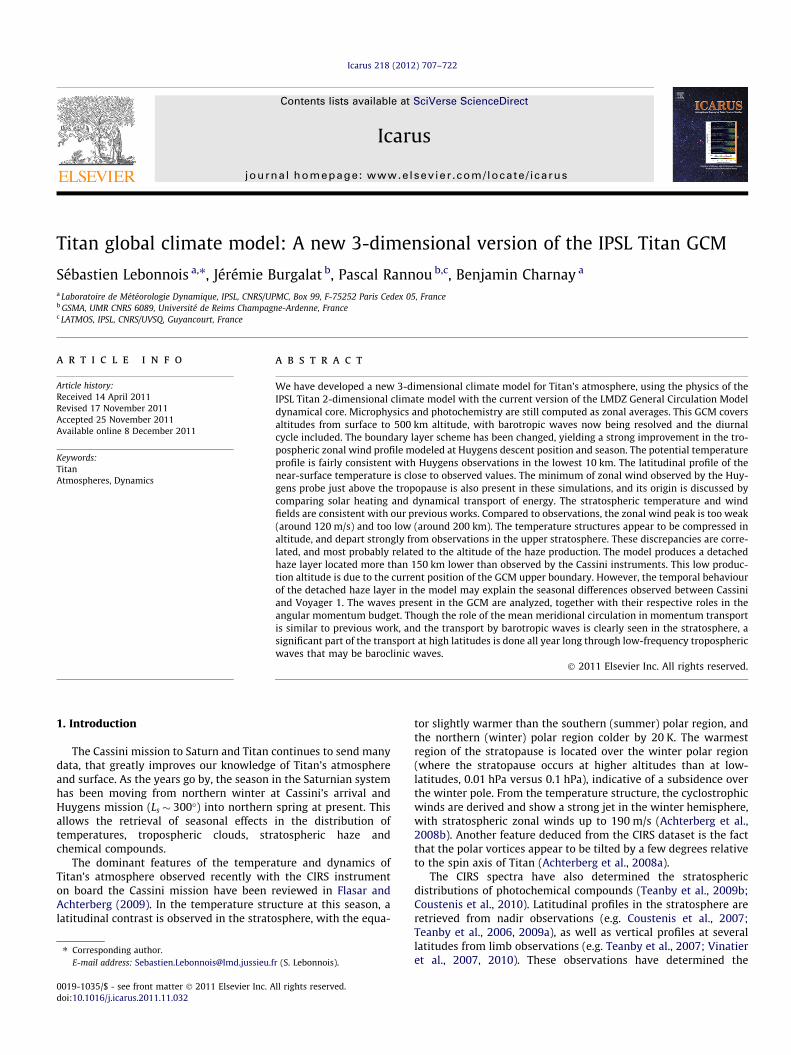
Fig. 12. Seasonal variations of the latitudinal transport of angular momentum by (a) mean meridional circulation and (b) transient waves. Unit is 103 m3/s2, positive valuesare northward.

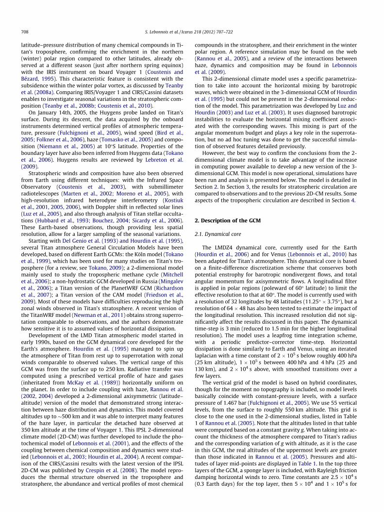
Fig. 13. Zonally averaged amplitude frequency spectrum for the zonal and meridional wind fields as a function of latitude, at pressure levels of 10 and 100 Pa. Chosen seasonis Ls = 295�. The solid curve is the mean zonal rotation speed of the flow (same unit as the frequency).



@

@z2Xu sin /þ u2 tan /

a

� �¼ � g

Ta@T@/

; ð1Þ

where a = 2.575 � 106 m is the radius of Titan, X = 4.56 � 10�6 s�1

is the rotation rate of Titan, / is the latitude, g = 1.35 m s�2 is thegravity, z (m) is the altitude, T (K) is the temperature and u(m s�1) is the zonal wind speed. This equation is presented herein the thin atmosphere approximation. It is further approximatedto link DT

D/ to DuDz:

�DuDz

2X sin /þ 2u tan /a

� �¼ g

TaDTD/

: ð2Þ

In the GCM simulation presented in this work, the followingvalues are estimated: u � 16 m s�1, T � 90 K, / � p/12 (averagedvalue for the region between the equator and 30�),Du � �4 m s�1, Dz � 1 � 104 m, DT � 0.2 K and D/ � p/6. Thefirst term evaluates to

�DuDz

2X sin /þ 2u tan /a

� �¼ 2:3� 10�9 s�2:

The second term evaluates to

gTa

DTD/¼ 2:2� 10�9 s�2:

Given the approximations done, the agreement is quite good,confirming that the zonal wind and temperature fields are relatedthrough the thermal wind equation. If we apply the same calcula-

Fig. 14. Zonally averaged amplitude frequency spectrum for the zonal and meridional wThe solid curve is the mean zonal rotation speed of the flow (same unit as the frequenc

tion to the observed profile, with u � 20 m s�1 (averaged value inthe decrease region), T � 90 K, Du � �40 m s�1, Dz � 1.5 � 104 m,and / � sin / � tan / � D/

2 , DT may be evaluated as

DT ¼ �DuDz

Xþ ua

� � TagðD/Þ2; ð3Þ

i.e.

DT ¼ 5:65� ðD/Þ2:

If the meridional temperature inversion is located betweenequator and mid-latitudes (D/ between 30 and 45�), this relationshould yield a latitudinal contrast in temperature around 1.5–3.5 K. This may be possible to observe with the Cassini radio-occul-tation data (Schinder et al., 2011).

Fig. 10 shows the annual average of the solar heating rates,heating due to dynamics, and cooling by infrared radiation (thesethree tendencies are balanced). Between the tropopause and70 km, the solar heating at equator is compensated by the coolingdue to ascending motions, resulting in a slightly lower coolingneeded around equator than at mid-latitudes. Therefore, our modelsuggests that this relative distribution of solar heating versusdynamical tendencies forces a local minimum of temperature inthis region. Through the thermal wind equation, this local mini-mum induces a decrease in zonal wind with altitude, thereforedriving the local minimum in zonal winds.

ind fields as a function of pressure, at equator and 60�N. Chosen season is Ls = 295�.y). The altitude scale on the right axis is approximate.


3.4. Transport of angular momentum and waves

Averaged over 1 Titan year, the transport of angular momentumis quite similar to previous models (such as Hourdin et al., 1995).Here, the angular momentum transport is computed for each lati-tude / as the integral over longitude k and pressure p of the quan-tity vua cos /dm, where dm is the element of mass (dm = a2cos /d/dkdp/g), normalized by the mass:

Rvua cos /dmR

dmðexpressed in m3

=s2Þ:

As shown in Fig. 11, the overall poleward transport of angularmomentum by the mean meridional circulation (MMC) is partiallycompensated through transport by waves in the low- to mid-lati-tudes. Poleward of roughly 40�, angular momentum is transportedtoward poles both by transient waves and by the mean meridionalcirculation. The total poleward transport is balanced by exchangesof angular momentum between the surface and the atmosphere.The zonally and annually averaged zonal wind at the surface isnegative below 30� latitude (transferring momentum from the sur-face into the atmosphere) and positive above (giving back momen-tum to the surface), as shown in Fig. 7. Fig. 12 shows the seasonalvariations of the transport by the MMC and waves. The evolution ofthe MMC transport is consistent with the seasonal variations of theHadley cells. The transport by transient waves follows a more com-plex pattern: at mid- to high-latitudes, the transport is continu-ously poleward, while between 40�N and 40�S, it is directed

Fig. 15. Latitude–altitude distribution of the maximum amplitude of the transients inLs = 295�. (a and c) Amplitude on zonal wind, the solid contours are the latitudinal gradwind, the solid contours are the mean zonal wind field (in m/s).

towards the spring/summer pole, stronger in the autumn/winterhemisphere where it counteracts the transport by the MMC, andreversing a third of season after the equinox. Significant variabilityis apparent in this horizontal transport by transients. This is consis-tent with the results of Newman et al. (2011), who find that strato-spheric waves transporting angular momentum are particularlyactive during some episodes in the fall and winter seasons.

To analyze the waves present in our simulation, high-frequencyoutput was recorded for 16 Titan days, 50 points per day, atLs � 295� where strong wave activity is visible. The eddy compo-nents of u and v at a given point in the atmosphere (u0(t) andv0(t)) were computed as the difference between the fields u(t)and v(t) and their time average at this point. For each point inthe atmosphere, a fast fourier transform was then performed onu0(t) and v0(t) after multiplication by a triangle function to limitthe impact of the time window. The distribution of waves is illus-trated in Fig. 13 at fixed pressures (10 and 100 Pa), and in Fig. 14 atfixed latitudes (equator and 60�N).

The most visible groups of waves in the u0 fields are locatedaround frequencies of �6 cycles/Titan day (thereafter f1) and�11 cycles/Titan day (thereafter f2), though above 100 Pa, thewaves are more widely distributed in frequency. For v0, the f1 waveis the most visible feature. The amplitudes of u0 and v0 around thesetwo frequencies are shown in the meridional plane in Fig. 15. Mostactivity is located in the 103–10 Pa pressure range, where the zonalwind jet is present, and at latitudes from 30�S to the northern(winter) pole, with u0 peaking near the equator while v0 is peakingin mid-latitudes. The latitudinal gradient of the absolute vorticity

the frequency ranges 5–7 cycles/Titan day (f1) and 10–12 cycles/Titan day (f2) atient of the absolute vorticity (in 10�11 m�1s�1). (b and d) Amplitude on meridional


@q@y¼ @

a@/2X sin /� @u

a@/

� �ð4Þ

(where q is the zonal average of q, the absolute vorticity) is used as acriterion for barotropic instabilities (Rayleigh-Kuo criterion, Kuo,1949; Vallis, 2006): it must change sign in the region of instability.Fig. 15 confirms that the region where the waves are the mostactive is also a region where @q

@y is low and often changes sign. There-fore it is probable that these waves are barotropic in nature. Fig. 15recalls work by Luz and Hourdin (2003) and Luz et al. (2003) (e.g.Fig. 15 of Luz et al. (2003)) in which the latitudinal gradient of po-tential vorticity was used to parameterize the eddy momentumtransport in the IPSL 2D-CM. This confirms that instabilities in the2D-CM and 3D GCM have similar distributions (and similar conse-quences in terms of angular momentum transport). The distributionof the f1 wave shows a significant activity on the poleward side ofthe jet, compared to f2.

To better investigate the role of each wave in the transport ofangular momentum in this simulation, the transients have beenseparated into three frequency regions, using filters applied onthe spectra: waves with frequencies lower than 4 cycles/Titan day(f0), waves with frequencies between 4 and 8 cycles/Titan day (i.e.mainly f1), and waves with larger frequencies (i.e. mainly f2). Instan-taneous horizontal field snapshots of filtered u0 are plotted inFig. 16. The chosen pressures correspond to regions of high ampli-tudes for each of these waves: around 200 Pa for f2, around 103 Pafor f1, and very close to the surface for f0 (1.3 � 105 Pa). The strato-spheric waves have wavenumber 1, while the f0 tropospheric wave

(a)

(c)

Fig. 16. Snapshots of the horizontal field of filtered perturbations on the zonal wind,stratosphere, at 103 Pa; (c) u0(f2) in the stratosphere, at 200 Pa.

has higher wavenumbers. All these waves are eastward propagat-ing. The dominant f0 wave seen at southern mid-latitudes inFig. 16a has a very low-frequency, around 0.2 cycles/Titan day.The stratospheric waves present very similar characteristics tothe waves displayed in Newman et al. (2011), which had frequen-cies from around 5 cycles/Titan day during spin-up to around16 cycles/Titan day at the end of their simulation.

In the regions where the f0 wave is active, the zonal wind u issteadily increasing with altitude. Here, close to the surface, thedynamical regime is more baroclinic. A criterion similar to the Ray-leigh-Kuo criterion for barotropic instabilities may be used to seewhether baroclinic instabilities can grow: the latitudinal gradientof the absolute vorticity @q

@y must change sign in the vertical direc-tion (Holton, 1992; Vallis, 2006). This is visible in the structurespresent in the troposphere in Fig. 15, close to the surface and closeto the pole. This reinforces the hypothesis that the tropospheric f0

waves are baroclinic in nature. Note that baroclinic instabilitieswere seen at high latitudes in simulations of superrotatingatmospheres done by Mitchell and Vallis (2010), for intermediatethermal Rossby numbers. Near-surface waves have also recentlybeen analyzed in a tropospheric Titan GCM simulation (Mitchellet al., 2011), in which they are connected to the precipitation pat-terns observed near equinox (Turtle et al., 2011). Mitchell et al.(2011) obtained mainly two wave modes, equatorial Kelvin wavesand mid-latitude waves propagating westward, confined near thesurface and presenting similarities with the waves we obtain here(though the f0 waves presented in Fig. 16a are slowly propagatingeastward, not westward).

(b)

at Ls = 295�. (a) u0(f0) in the lower troposphere, at 1.3 � 105 Pa; (b) u0(f1) in the


The transport of angular momentum by each family of waves iscomputed using the filtered u0 and v0, and presented in Fig. 17,where it is split between upper atmosphere, stratosphere and tro-posphere. This transport is composed of two main components.The stratospheric waves (both f1 and f2 equally) transport a signif-icant amount of angular momentum in the direction opposing themean meridional circulation, especially during the solstice season.This transport also appears at low- to mid-latitudes in Figs. 11 and12b. However, another component of the transport appears inFig. 17: this is done by the low-frequency waves in the tropo-sphere, at mid-to high-latitudes, despite their very low amplitude.This transport is directed towards the pole and is present even inperiods of low barotropic wave activity. This component explainsmost of the transport seen poleward of 40� latitude in Figs. 11and 12b.

To verify whether the high-latitude tropospheric componentwas related to the solar thermal tide, we have run a 1-year simu-lation without the diurnal cycle. During this year, the transportof angular momentum is not much affected; the same two compo-nents are found in the transport by waves, and the circulation isvery similar to the nominal simulation with a diurnal cycle. Thisresult is consistent with the small impact of the diurnal cycle ob-tained in Hourdin et al. (1995) and confirms that the high-latitudetropospheric transport in our simulations is not related to the solarthermal tide.

(a)

(c)

Fig. 17. Latitudinal transport of angular momentum in the simulation at Ls = 295�, for mday, dotted lines), transients with frequencies between 4 and 8 cycle/Titan day (i.e. mainlf2, dash-dotted lines). In panel (a), the relative angular momentum latitudinal transport isthe column. In the other panels, it is integrated only for a fraction of the column, but it is splot (a). Unit is 103 m3/s2, positive values are northward.

4. Results in the troposphere

The annual cycles of temperature at the surface and at the tro-popause are shown in Fig. 18. The surface temperature is roughly1 K below the value observed by Huygens (93.65 K, Fulchignoniet al., 2005), and the latitudinal contrast between winter polar re-gions and equator (around 2 K), as well as between summer polarregions and equator (around 0.6 K) are both under-estimated com-pared to the values retrieved by Jennings et al. (2009) (respectively3 K and 2 K). The contrasts seen after northern spring equinox(1.5–2 K, almost symmetric) are consistent with IRIS/Voyager 1observations. The modeled temperature at tropopause is very closeto the Huygens observed value (70.4 K, Fulchignoni et al., 2005)and does not vary appreciably with either latitude or season. Whenthe surface thermal inertia is reduced to I = 340 J m�2 s�0.5 K�1, thetemporal variations of both surface and tropopause temperaturesare slightly enhanced, and the temporal evolution of the surfacemaximum temperature is modified, with the maximum atLs � 300� displaced towards southern mid-latitudes.

The vertical profile of potential temperature at the Huygenslanding site (Tokano et al., 2006, Fig. 2) shows an increase ofroughly 5 K in the last 10 km, with a well-mixed boundary layerconfined to 300 m above the surface. Shoulders in the profile arealso seen around 800 m and 3 km altitude. A 2–3 km boundarylayer is also consistent with dune spacing, as shown in Lorenz

(b)

(d)

ean meridional circulation (solid lines), low-frequency transients (0–4 cycles/Titany f1, dashed lines) and high-frequency transients (above 8 cycle/Titan day, i.e. mainly

integrated for the entire column at each latitude, and is divided by the total mass oftill divided by the total mass of the entire column, so that the three plots add to give

Fig. 18. Annual variations of the zonally averaged latitudinal temperature profile at(a) surface and (b) tropopause (roughly 40 km altitude).

Fig. 19. Potential temperature vertical profile at 10�S (zonal average) and Ls = 300�,corresponding to the Huygens descent. The HASI/Huygens potential temperatureprofile is also shown (bold line).


et al. (2010). In Fig. 19, the diurnally averaged potential tempera-ture profile in the GCM is shown for the deepest 10 km, at the Huy-gens landing site and season, together with the Huygens profile.The simulated boundary layer is located in the deepest 2 km, withan increase of 7 K between the surface and 10 km altitude. A de-tailed analysis of the diurnal and seasonal evolution of this near-surface potential temperature profile appears in a dedicated study(Charnay and Lebonnois, 2011). The modeled surface temperatureat this point (and also its latitudinal profile) is sensitive to thechoices of thermal inertia and albedo, and is also sensitive to thevertical distribution of haze. Clouds (not included here) may alsoaffect the surface temperature.

The profiles of diurnally averaged zonal and meridional windsin the troposphere at the Huygens landing site have been retrievedfrom the probe’s trajectory (Tokano, 2009, Fig. 2). These are showntogether with the modeled wind profiles at the same location andseason in Fig. 20. As seen in Fig. 9, the vertical profile of the zonalwind in the troposphere is in very good agreement with the mea-surements of the Huygens probe. Just above the surface, the wind

is slightly positive (eastward), though it is mostly negative in thedeepest 5 km, as in the observations. However, the amplitude ofthis westward wind is approximately half of the observed value.When reduced thermal inertia is used, the amplitude of wind vari-ations are enhanced, and the retrograde region (negative u) per-sists up to 7–8 km.

The comparison between model and observations is less satis-factory for the meridional wind. Southward wind (negative) is in-deed obtained just above the surface, but again the amplitude isonly half the observed value. Between 1 and 5 km, both observedand modeled winds are northward, though modeled values aremuch less than observations. Above 3 km, the modeled meridionalwind is almost zero up to the tropopause. The northward andsouthward winds present in the observations above 5 km are notobtained in the simulation. However, this observed profile corre-sponds to an instantaneous profile where waves and topographiceffects may have been present.

Specific studies dedicated to the troposphere are underway andwill be presented in future papers.

5. Conclusion

Based on the current version of the LMDZ Earth GeneralCirculation Model dynamical core, we have developed a new mod-el of Titan’s atmosphere, including physic parametrizations fromthe IPSL 2-dimensional Titan Climate Model (2D-CM). However,due to computational limitations, microphysics of the haze andphotochemistry are still computed as zonal averages. The newGCM simulation presented in this work has been initialized withthe 2D-CM reference state at northern spring equinox and runfor 12 Titan years.

Comparing this new simulation to previous 2-dimensionalsimulations and to observations, the following conclusions maybe drawn:

� The modeled temperature structure is fairly similar betweenboth models, with the same problems in the upper stratospherewhere the temperatures are too cold, and above the 10 hPa level(approximately 300 km altitude) where no stratopause isobtained and the temperature is not realistic compared toobservations. As in the 2D-CM, this is presumably related tothe limitations of the radiative transfer and to the upper bound-ary position, which limits the altitude of the haze productionregion.

(a) (b)

Fig. 20. Zonal (a) and meridional (b) wind vertical profiles at 10�S (zonal average) and Ls = 300�, corresponding to the Huygens descent. Values computed from the Huygensdescent trajectory dataset (Tokano, 2009) are also plotted (bold lines).


� The comparison to observed latitudinal profiles of temperaturein the lower stratosphere shows that the overall modeled tem-perature structure appears compressed in altitude. In spring,the comparison is not as good as for the 2D-CM, probablybecause of the haze distribution.� The detached haze layer is present most of the year, lower than

observed as in the 2D-CM. It shrinks and disappears after equi-nox, due to the shift of the ascending region from one pole tothe other. The altitude difference between Cassini and Voyager1 observations is a seasonal effect, now confirmed by the Cas-sini monitoring of the detached haze layer over the equinox(West et al., 2011). Comparing simulations with observationsof this transition period should help to clarify the interactionbetween the haze and the atmospheric circulation.� The zonal wind peak modeled at Cassini season is lower in

amplitude as well as in altitude in this new simulation com-pared to the 2D-CM. However, the temporal evolution of thezonal wind field is qualitatively consistent with availableobservations.� Changing the planetary boundary layer scheme has greatly

improved agreement between the model and the troposphericprofile of the zonal wind from the Huygens descent.� As in previous LMD models, a minimum in the zonal wind field

is obtained close to the region where Huygens observed a stron-ger minimum in the equatorial lower stratosphere. In the simu-lation, this minimum is correlated with a local minimum in thetemperature field, due to the relative distributions of solar forc-ing and dynamical transport of energy. According to the thermalwind equation, the observed wind minimum could correspondto an equatorial temperature around 2 K lower than mid-lati-tudes at 20–40 hPa (60–75 km altitude). This region is also cor-related with a reversal (change of sign) of the meridional wind.� In this 3D simulation, the diurnal cycle has been taken into

account, but its role is minor. Barotropic instabilities, diagnosedand parameterized in the 2D-CM, are now explicitely simulatedand many waves are visible in the stratosphere, mostly in theregion around the zonal wind maximum. The horizontal trans-port of angular momentum by the mean meridional circulationis similar to the 2D simulation. However, the transport bytransient waves is more complicated than in previous work.Barotropic waves transport momentum opposite to meanmeridional circulation in mid- to low-latitudes, but a secondcomponent of the momentum transport appears at mid- to

high-latitudes, due to low-frequency waves located close tothe surface. Instability criterion as well as the more barocliniccharacteristics of this region indicate that these waves are baro-clinic waves. They transport momentum poleward at high lati-tudes all year long.� In the lower troposphere, simulated potential temperature,

zonal and meridional winds are compared to Huygens descentprofiles. Though the amplitudes of wind variations are smallerthan observed, the vertical profiles are very similar, except forthe meridional wind above 3 km. Near-surface behavior of themodel is sensitive to uncertain input parameters such as albedoand thermal inertia.

Due to the complex coupling between dynamics, haze particlesand radiative transfer, it is difficult to adjust model parameters toget a circulation that fits observations everywhere. The modelneeds to be improved, especially above 300 km altitude wherethe temperature structure is far from observations. This affectsthe top of the haze layer as well as its time variability, and theresulting zonal wind structure and temperature distributions.The upgrade of the radiative transfer module in the GCM and thevertical extension of the upper boundary are underway and shouldhelp improve this situation.

Acknowledgements

The authors thank Frederic Hourdin for very useful discussionson the model and on this paper. This work has been supported bythe project Exoclimats financed by the Agence Nationale de laRecherche (ANR), and by the computation facilities of both theInstitut du Développement et des Ressources en Informatique Sci-entifique (IDRIS) and the University Pierre and Marie Curie(UPMC).

References

Achterberg, R.K., Conrath, B.J., Gierasch, P.J., Flasar, F.M., Nixon, C.A., 2008a.Observation of a tilt of Titan’s middle-atmospheric superrotation. Icarus 197,549–555.

Achterberg, R.K., Conrath, B.J., Gierasch, P.J., Flasar, F.M., Nixon, C.A., 2008b. Titan’smiddle-atmospheric temperatures and dynamics observed by the CassiniComposite Infrared Spectrometer. Icarus 194, 263–277.

Bird, M.K. et al., 2005. The vertical profile of winds on Titan. Nature 438, 1–3.Bouchez, A., 2004. Seasonal Trends in Titan’s Atmosphere: Haze, Winds, and Clouds.

Ph.D. thesis. California Institute of Technology.


Charnay, B., Lebonnois, S., 2011. Thermal structure and dynamics of Titan’s lowertroposphere. Nat. Geosci., in press.

Coustenis, A., Bézard, B., 1995. Titan’s atmosphere from Voyager infraredobservations. IV. Latitudinal variations of temperature and composition.Icarus 115, 126–140.

Coustenis, A. et al., 2003. Titan’s atmosphere from ISO mid-infrared spectroscopy.Icarus 161, 383–403.

Coustenis, A. et al., 2007. The composition of Titan’s stratosphere from Cassini/CIRSmid-infrared spectra. Icarus 189, 35–62.

Coustenis, A., Jennings, D., Nixon, C., Achterberg, R.K., Lavvas, P., Vinatier, S., Teanby,N.A., Bjoraker, G.L., Carlson, R.C., Piani, L., Bampasidis, G., Flasar, F.M., Romani,P.N., 2010. Titan trace gaseous composition from CIRS at the end of the Cassini–Huygens prime mission. Icarus 207, 461–476.

Crespin, A., Lebonnois, S., Vinatier, S., Bézard, B., Coustenis, A., Teanby, N.A.,Achterberg, R.K., Rannou, P., Hourdin, F., 2008. Diagnostics of Titan’sstratospheric dynamics using Cassini/CIRS data and the IPSL GeneralCirculation Model. Icarus 197, 556–571.

Del Genio, A.D., Zhou, W., Eichler, T.P., 1993. Equatorial superrotation in a slowlyrotating GCM: Implications for Titan and Venus. Icarus 101, 1–17.

Flasar, F.M. et al., 2005. Titan’s atmospheric temperatures, winds, and composition.Science 308, 975–978.

Flasar, F.M., Achterberg, R.K., 2009. The structure and dynamics of Titan’s middleatmosphere. Philos. Trans. Roy. Soc. A 367, 649–664.

Flasar, F.M., Samuelson, R.E., Conrath, B.J., 1981. Titan’s atmosphere: Temperatureand dynamics. Nature 292, 693–698.

Folkner, W.M. et al., 2006. Winds on Titan from ground-based tracking of theHuygens probe. J. Geophys. Res. 111, E07S02.

Friedson, A.J., West, R.A., Wilson, E.H., Oyafuso, F., Orton, G.S., 2009. A global climatemodel of Titan’s atmosphere and surface. Planet. Space Sci. 57, 1931–1949.

Fulchignoni, M. et al., 2005. In situ measurements of the physical characteristics ofTitan’s environment. Nature 438, 1–7.

Holton, J.R., 1992. An introduction to dynamic meteorology. In: InternationalGeophysics Series, third ed. Academic Press, San Diego, New York.

Hourdin, F. et al., 2006. The LMDZ4 general circulation model: Climate performanceand sensitivity to parameterized physics with emphasis on tropical convection.Clim. Dyn. 27, 787–813.

Hourdin, F., Le Van, P., Forget, F., Talagrand, O., 1993. Meteorological variability andthe annual surface pressure cycle on Mars. J. Atmos. Sci. 50, 3625–3640.

Hourdin, F., Talagrand, O., Sadourny, R., Courtin, R., Gautier, D., McKay, C.P., 1995.Numerical simulation of the general circulation of the atmosphere of Titan.Icarus 117, 358–374.

Hourdin, F., Couvreux, F., Menut, L., 2002. Parameterization of the dry convectiveboundary layer based on a mass flux representation of thermals. J. Atmos. Sci.59, 1105–1123.

Hourdin, F., Lebonnois, S., Luz, D., Rannou, P., 2004. Titan’s stratosphericcomposition driven by condensation and dynamics. J. Geophys. Res. 109,E12005.

Hubbard, W.B. et al., 1993. The occultation of 28 Sgr by Titan. Astron. Astrophys.269, 541–563.

Jennings, D.E. et al., 2009. Titan’s surface brightness temperatures. Astrophys. J. 691,L103–L105.

Kostiuk, T. et al., 2001. Direct measurements of winds on Titan. Geophys. Res. Lett.28, 2361–2364.

Kostiuk, T. et al., 2005. Titan’s stratospheric zonal wind, temperature, and ethaneabundance a year prior to Huygens insertion. Geophys. Res. Lett. 32, L22205.

Kostiuk, T. et al., 2006. Stratospheric global winds on Titan at the time of Huygensdescent. J. Geophys. Res. 111, E07S03.

Kostiuk, T. et al., 2010. High spectral resolution infrared studies of Titan: Winds,temperature, and composition. Planet. Space Sci. 58, 1715–1723.

Kuo, H.I., 1949. Dynamic instability of 2-dimensional nondivergent flow in abarotropic atmosphere. J. Meteor. 6, 105–122.

Lebonnois, S., Toublanc, D., Hourdin, F., Rannou, P., 2001. Seasonal variations inTitan’s atmospheric composition. Icarus 152, 384–406.

Lebonnois, S., Hourdin, F., Rannou, P., Luz, D., Toublanc, D., 2003. Impact of theseasonal variations of ethane and acetylene distributions on the temperaturefield of Titan’s stratosphere. Icarus 163, 164–174.

Lebonnois, S., Hourdin, F., Rannou, P., 2009. The coupling of winds, aerosols andphotochemistry in Titan’s atmosphere. Philos. Trans. Roy. Soc. A 367, 665–682.

Lebonnois, S., Hourdin, F., Eymet, V., Crespin, A., Fournier, R., Forget, F., 2010.Superrotation of Venus’ atmosphere analysed with a full General CirculationModel. J. Geophys. Res. 115, E06006.

Lebonnois, S. et al., 2011. A comparative analysis of simplified general circulationmodels of Venus atmosphere. In: Towards Understanding the Climate of Venus:Application of Terrestrial Models to Our Sister Planet. Springer, Netherlands, inpress.

Lebreton, J.P., Coustenis, A., Lunine, J., Raulin, F., Owen, T., Strobel, D., 2009. Resultsfrom the Huygens probe on Titan. Astron. Astrophys. Rev. 17, 149–179.

Lorenz, R.D., Claudin, P., Andreotti, B., Radebaugh, J., Tokano, T., 2010. A 3 kmatmospheric boundary layer on Titan indicated by dune spacing and Huygensdata. Icarus 205, 719–721.

Luz, D., Hourdin, F., 2003. Latitudinal transport by barotropic waves in Titan’sstratosphere. I. General properties from a horizontal shallow-water model.Icarus 166, 328–342.

Luz, D., Hourdin, F., Rannou, P., Lebonnois, S., 2003. Latitudinal transport bybarotropic waves in Titan’s stratosphere. II. Results from a coupled dynamics–microphysics–photochemistry GCM. Icarus 166, 343–358.

Luz, D., Civeit, T.R.C., Lebreton, J.P., Gautier, D., Rannou, P., Kaufer, A., Witasse, O.,Lara, L., Ferri, F., 2005. Characterization of zonal winds in the stratosphere ofTitan with UVES. Icarus 179, 497–510.

Marten, A., Hidayat, T., Biraud, Y., Moreno, R., 2002. New millimeter heterodyneobservations of Titan: Vertical distributions of nitriles HCN, HC3N, CH3CN, andthe isotopic ratio 15N/14N in its atmosphere. Icarus 158, 532–544.

McKay, C.P., Pollack, J.B., Courtin, R., 1989. The thermal structure of Titan’satmosphere. Icarus 80, 23–53.

Mellor, G.L., Yamada, T., 1982. Development of a turbulent closure model forgeophysical fluid problems. Rev. Geophys. Space Phys. 20, 851–875.

Mingalev, I.V. et al., 2006. First simulation results of Titan’s atmospheric dynamicswith a global 3-D non-hydrostatic circulation model. Ann. Geophys. 24, 1–15.

Mitchell, J.L., Vallis, G.K., 2010. The transition to superrotation in terrestrialatmospheres. J. Geophys. Res. 115, E12008.

Mitchell, J.L., Pierrehumbert, R.T., Frierson, D., Caballero, R., 2006. The dynamicsbehind Titan’s methane cloud. Proc. Nat. Acad. Sci. 103, 18421–18426.

Mitchell, J.L., Ádámkovics, M., Caballero, R., Turtle, E.P., 2011. Locally enhancedprecipitation organized by planetary-scale waves on Titan. Nat. Geosci. 4, 589–592.

Moreno, R., Marten, A., Hidayat, T., 2005. Interferometric measurements of zonalwinds on Titan. Astron. Astrophys. 437, 319–328.

Newman, C.E., Lee, C., Lian, Y., Richardson, M.I., Toigo, A.D., 2011. Stratosphericsuperrotation in the TitanWRF model. Icarus 213, 636–654.

Niemann, H.B. et al., 2005. The abundances of constituents of Titan’s atmospherefrom the GCMS instrument on the Huygens probe. Nature 438, 1–6.

Rannou, P., Hourdin, F., McKay, C.P., 2002. A wind origin for Titan’s haze structure.Nature 418, 853–856.

Rannou, P., Hourdin, F., McKay, C.P., Luz, D., 2004. A coupled dynamics-microphysics model of Titan’s atmosphere. Icarus 170, 443–462.

Rannou, P., Lebonnois, S., Hourdin, F., Luz, D., 2005. Titan atmosphere database. Adv.Space Res. 36, 2194–2198.

Rannou, P., Montmessin, F., Hourdin, F., Lebonnois, S., 2006. The latitudinaldistribution of clouds on Titan. Science 311, 201–205.

Richardson, M.I., Toigo, A.D., Newman, C.E., 2007. PlanetWRF: A general purpose,local to global numerical model for planetary atmospheric and climatedynamics. J. Geophys. Res. 112, E09001.

Schinder, P.J., Flasar, F.M., Marouf, E.A., French, R.G., McGhee, C.A., Kliore, A.J.,Rappaport, N.J., Barbinis, E., Fleischman, D., Anabtawi, A., 2011. The structure ofTitan’s atmosphere from Cassini radio occultations. Icarus 215, 460–474.

Sicardy, B. et al., 2006. The two Titan stellar occultations of 14 November 2003. J.Geophys. Res. 111, E11S91.

Teanby, N.A. et al., 2008a. Titan’s winter polar vortex structure revealed by chemicaltracers. J. Geophys. Res. 113, E12003.

Teanby, N.A., Irwin, P.G.J., de Kok, R., Nixon, C.A., Coustenis, A., Bézard, B., Calcutt,S.B., Bowles, N.E., Flasar, F.M., Fletcher, L., Howett, C., Taylor, F.W., 2006.Latitudinal variations of HCN, HC3N and C2N2 in Titan’s stratosphere derivedfrom Cassini CIRS data. Icarus 181, 243–255.

Teanby, N.A., Irwin, P.G.J., de Kok, R., Vinatier, S., Bézard, B., Nixon, C.A., Flasar, F.M.,Calcutt, S.B., Bowles, N.E., Fletcher, L., Howett, C., Taylor, F.W., 2007. Verticalprofiles of HCN, HC3N and C2H2 in Titan’s atmosphere derived from Cassini/CIRSdata. Icarus 186, 364–384.

Teanby, N.A., Irwin, P.G.J., de Kok, R., Nixon, C.A., Coustenis, A., Royer, E., Calcutt, S.B.,Bowles, N.E., Fletcher, L., Howett, C., Taylor, F.W., 2008b. Global and temporalvariations in hydrocarbons and nitriles in Titan’s stratosphere for northernwinter observed by Cassini/CIRS. Icarus 193, 595–611.

Teanby, N.A., Irwin, P.G.J., de Kok, R., Jolly, A., Bézard, B., Nixon, C.A., Calcutt, S.B.,2009a. Titan’s stratospheric C2N2, C3H4 and C4H2 abundances from Cassini/CIRSfar-infrared spectra. Icarus 202, 620–631.

Teanby, N.A., Irwin, P.G.J., de Kok, R., Nixon, C.A., 2009b. Dynamical implications ofseasonal and spatial variations in Titan’s stratospheric composition. Philos.Trans. Roy. Soc. A 367, 697–711.

Tokano, T., 2009. The dynamics of Titan’s troposphere. Philos. Trans. Roy. Soc. A 367,633–648.

Tokano, T., Neubauer, F.M., Laube, M., McKay, C.P., 1999. Seasonal variation ofTitan’s atmospheric structure simulated by a general circulation model. Planet.Space Sci. 47, 493–520.

Tokano, T., Ferri, F., Colombatti, G., Mäkinen, T., Fulchignoni, M., 2006. Titan’splanetary boundary layer structure at the Huygens landing site. J. Geophys. Res.111, E08007.

Tomasko, M.G. et al., 2005. Rain, winds and haze during the Huygens probe’sdescent to Titan’s surface. Nature 438, 1–14.

Turtle, E.P. et al., 2011. Seasonal changes in Titan’s meteorology. Geophys. Res. Lett.38, L03203.

Vallis, G.K., 2006. Atmospheric and Oceanic Fluid Dynamics. Cambridge UniversityPress, Cambridge, UK.

Vinatier, S., Bézard, B., Fouchet, T., Teanby, N.A., de Kok, R., Irwin, P., Conrath, B.J.,Nixon, C.A., Romani, P.N., Flasar, F.M., Coustenis, A., 2007. Vertical abundanceprofiles of hydrocarbons in Titan’s atmosphere at 15�S and 80�N retrieved fromCassini/CIRS spectra. Icarus 188, 120–138.

Vinatier, S., Bézard, B., Nixon, C.A., Mamoutkine, A., Carlson, R.C., Jennings, E.D.,Guandique, E.A., Teanby, N.A., Bjoraker, G.L., Flasar, F.M., Kunde, V.G., 2010.Analysis of Cassini/CIRS spectra of Titan acquired during the nominal mission. I.Hydrocarbons, nitriles and CO2 vertical mixing ratio profiles. Icarus 205, 559–570.

West, R.A. et al., 2011. The evolution of Titan’s detached haze layer near equinox in2009. Geophys. Res. Lett. 380, L06204.

Titan global climate model: A new 3-dimensional version of ...

Documents

Transcript of Titan global climate model: A new 3-dimensional version of ...