Tire-soil interaction analysis of forest machines Karthik ...

Tire-soil interaction analysis of forest

machines

Karthik Prakash

Master of Science Thesis MMK 2014:15 MKN 105

KTH Industrial Engineering and Management

Machine Design

SE-100 44 STOCKHOLM

1

Examensarbete MMK 2014:15 MKN 105

Analys av däck-maskinteraktionen hos

skogmaskiner

Karthik Prakash

Godkänt

2014-06-04

Examinator

Ulf Sellgren

Handledare

Ulf Sellgren

Uppdragsgivare

Skogforsk

Kontaktperson

Björn Löfgren

Sammanfattning

Kortvirkesmetoden är en mekaniserad för skogsavverkning. Det är en två-maskinsprocess,

som utförs av en skördare och en skotare. Skotaren kan orsaka skador på marken, som

exempelvis spårbildning och markpackning. Det har blivit allt viktigare att skydda skogen

från de marskador orsakade av tunga maskiner. Detta är en initiell studie av samspelet mellan

mark och hjul på en lastad skotare.

Olika WES-baserade spårdjupsmodeller har jämförts för att värdera deras förmåga att

prediktera spårdjupen. Nya modeller har också utvecklats för att uppskatta relationen mellan

spårdjup och flera hjulpassager. Modeller som kan prediktera kontakttrycket mellan däcket

och marken, samt däckets markkontaktarea har studerats. Olika relationer för att bestämma

mobilitetsparametrarna har också studerats.

Rötter spelar en viktig roll för att öka markens bärighet och att skydda den. Rötternas effekt

på markens bärighet har behandlats i examensarbetet. Labbtester med tallrötter har

genomförts för att bestämma deras armeringseffekt. Modeller som kan användas för att

prediktera rötternas effekter har också studerats.

Ett första steg för att kunna kombinera WES- och Bekker-modeller har utförts, tillgängliga

modeller som korrelerar WES- och Bekker-modeller har behandlats och en uppsättning

relationer som relaterar de båda modellerna har härletts.

Effekten av halka i samband med nedsjunkning har studerats med hjälp av både WES- och

Bekkerbaserade modeller. Dynamiksimuleringsprogramet MSC Adams har använts för att

simulera skotarmodellen för att bestämma dess lämplighet för spårdjupsförutsägelse. Adams

har använts för att studera vilken effekt olika däcktryck och hastighet har på spårdjupet.

Nyckelord: Bekker, skogsmark, skotare, spårdjup, WES

3

Master of Science Thesis MMK 2014:15 MKN 105

Tire –soil interaction analysis of forest machines

Karthik Prakash

Approved

2014-06-04

Examiner

Ulf Sellgren

Supervisor

Ulf Sellgren

Commissioner

Skogforsk

Contact person

Björn Löfgren

Abstract

Cut-to-length logging is a mechanized method for delimbing trees and cutting them to length.

It is a two-machine operation; taken care by a harvester and a forwarder. The forwarder can

cause soil rutting, soil compaction and other detrimental after effects. Therefore it has become

vital to protect the forest floor from destructive effects of heavy machines. This initiated the

study to delve more into the interaction between the loaded forwarder wheel and the soil.

Various WES based rut depth models has been compared to validate its effectiveness in

predicting the rut depths. New models have been developed to estimate the rut depth produced

by the multipass effect of wheels. Models that could predict the contact pressure between the

tire and soil as well as the tire soil contact area has been studied. Various relations to

determine the mobility parameters have also been studied. The ones that are suitable to predict

mobility parameters have been identified.

Roots play a major role in reinforcing the soil and protecting them. This extra reinforcement

provided by roots has been taken into account in the thesis work. Lab test with pine tree roots

have been carried out to determine the extra reinforcement supplied. Models that are capable

of predicting the reinforcement effects due to roots have also been looked into.

An initial step towards connecting WES and Bekker models have been done; available models

correlating both WES and Bekker models have been analysed and finally a set of relations

connecting both have been derived.

The effect of slip on sinkage has been studied with the help of both WES and Bekker based

models. Multibody simulation software MSC Adams has been used to simulate the forwarder

model to determine its suitability for rut depth prediction. Adams has been employed to study

the effect of tire inflation pressure and velocity on rut depth.

Keywords: Bekker, forwarder, forest soil, rutting, WES

5

FOREWORD

I express my heartfelt gratitude to all the people who extended their unconditional support

and help during the course of the thesis work.

First and the foremost, I would like to express my sincere gratitude to Professor Ulf Sellgren,

my professor, the internal supervisor and more over an excellent mechanical engineer. The

guidance and suggestions provided by Ulf was a major source of inspiration to this work.

I thank Dr. Björn Löfgren from Skogforsk for believing in me to carry out this work. His

inputs during the pulse meetings were very constructive.

Abdurasul Pirnazarov, without this person the work would not have reached its final phase.

The insights he provided into the field of terramechanics is invaluable. I am indebted to

Abdurasul for spending long hours discussing various aspects of the projects and providing

valuable inputs. I would like to thank him from the bottom of my heart for all the help he has

done as well as for lending valuable literatures associated with the work.

I would like to thank Professor Kjell Andersson for all the help he provided during the Adams

modeling stage.

I express my sincere thanks to Abboos Ismailov for the help he offered during Adams

simulation.

Madura Wijekoon, R&D Product Development Coordinator in Trelleborg, is another person I

am indebted to for all the tire technical documents he provided. I greatly appreciate the

helping hand he provided to clear various doubts.

I thank Revathi Palaniappan for sorting all my queries associated with various aspects of the

project.

I am grateful to Praveen R. Nair for clearing various doubts associated with Adams

simulations.

I express my sincere gratitude and reverence towards my parents, C.M.Prakash and Haripriya

Prakash, for their unconditional love and support.

Finally, I dedicate this work to the Omnipotent and the Omnipresent for helping me to reach

this stage.

‘’If you perform the sacrifice of doing your duty, you do not have to do anything else. Devoted

to duty, man attains perfection.’’ – The Bhagavad Gita

Karthik Prakash

Stockholm, 06-2014

8

NOMENCLATURE

The abbreviations used in the thesis report are mentioned here

Abbreviations

ADAMS Automatic Dynamic Analysis of Mechanical Systems

ANN Artificial Neural Network

CI Cone Index

DEM Digital Elevation Model

DEM Discrete Element Method

FBM Fiber Bundle Model

FEM Finite Element Method/Finite Element Modelling

MBS Multi Body Simulation

MPC Multi-Pass Coefficient

NGP Nominal Ground Pressure

WES Waterways Experiment Station

WMR Wheeled Mobility Robots

10

TABLE OF CONTENTS

SAMMANFATTNING .............................................................................................................. 1

ABSTRACT ............................................................................................................................... 3

FOREWORD ............................................................................................................................. 5

NOMENCLATURE .................................................................................................................. 8

TABLE OF CONTENTS ........................................................................................................ 10

1 INTRODUCTION ............................................................................................................ 14

1.1 Background..................................................................................................................... 14

1.2 Purpose ........................................................................................................................... 16

1.3 Delimitations .................................................................................................................. 17

1.4 Method............................................................................................................................ 17

2 FRAME OF REFERENCE .............................................................................................. 18

2.1 Terramechanics............................................................................................................... 18

2.2 Tire-soil interaction models............................................................................................ 18

2.2.1 Empirical Models .................................................................................................... 19

2.2.2 Parametric analysis .................................................................................................. 21

2.3 Mathematical models...................................................................................................... 23

2.4 Computational models .................................................................................................... 23

2.5 Roots ............................................................................................................................... 24

2.5.1 Root reinforcement modelling................................................................................. 24

2.6 Soil Damage ................................................................................................................... 24

2.7 Multi-body simulation .................................................................................................... 25

2.7.1 Adams soft-soil tire and road models ...................................................................... 25

2.8 Digital soil modelling ..................................................................................................... 26

3 DATA COLLECTION ..................................................................................................... 27

3.1 Test machines ................................................................................................................. 27

3.2 Pressure measurement .................................................................................................... 27

3.3 Soil moisture................................................................................................................... 28

3.4 Soil penetration test ........................................................................................................ 28

3.5 Rut depth measurement .................................................................................................. 29

11

3.6 Tire-soil contact area ...................................................................................................... 30

3.7 Forwarder running gear description ............................................................................... 30

4 RUT DEPTH ANALYSIS ............................................................................................... 32

4.1 Introduction .................................................................................................................... 32

4.2 WES based rut depth models.......................................................................................... 32

4.3 Refinement of WES based rut depth models.................................................................. 35

4.3.1 Non-linear regression analysis ................................................................................ 35

4.3.2 Application of ‘novel wheel mobility number’ ....................................................... 37

4.3.3 Multi-pass rut depth models .................................................................................... 40

4.3.4 Rut depth estimation with changing Cone Index .................................................... 45

4.3.5 Rut depth estimation with Kharkhuta’s model ........................................................ 47

4.3.6 Change in rut depth with cone index ....................................................................... 48

4.3.7 Cone Index vs. Depth of measurement.................................................................... 49

5 PRESSURE MODELS ..................................................................................................... 52

6 Tire-Soil Contact Area ..................................................................................................... 57

6.1 Super ellipse as tire soil contact area.............................................................................. 60

7 Mobility Models ............................................................................................................... 62

7.1 Change of soil density and cohesion due to multi-pass.................................................. 66

8 TESTING WITH ROOTS ................................................................................................ 68

8.1 Laboratory root test’s ..................................................................................................... 68

8.2 Root reinforcement analysis ........................................................................................... 77

8.3 Rut depth comparison with and without roots................................................................ 81

8.4 Analysis of test data from lab root test ........................................................................... 83

8.5 Modelling roots as circular plate under elastic foundation and as plate under semi-

infinite solid. ......................................................................................................................... 84

9 Slip Sinkage Effect ........................................................................................................... 86

9.1 Estimating rut depth based on single wheel test............................................................. 88

10 Co-relating WES and Bevameter models ......................................................................... 90

11 ADAMS Multi-body Simulation ...................................................................................... 96

11.1 Adams Tire ................................................................................................................... 96

11.2 Soft-soil tire model ....................................................................................................... 98

11.3 Rigid wheel model........................................................................................................ 98

12

11.4 Elastic tire model .......................................................................................................... 98

11.5 Elastic/plastic deformation of the soil .......................................................................... 99

11.6 Visco-elastic tire soil contact........................................................................................ 99

11.7 Observations in Adams soft soil ................................................................................... 99

11.8 Multi-pass effect ......................................................................................................... 101

11.9 Connecting Adams results with WES models ............................................................ 102

11.10 Simulation of the Komatsu 860.3 model .................................................................. 105

11.11 Effect of tire inflation pressure on sinkage............................................................... 107

11.12 Effect of velocity on rut depth .................................................................................. 109

12 DISCUSSION AND CONCLUSIONS .......................................................................... 110

12.1 Rut depth .................................................................................................................... 110

12.2 Pressure....................................................................................................................... 112

12.3 Contact area ................................................................................................................ 114

12.4 Mobility parameters.................................................................................................... 114

12.5 Roots ........................................................................................................................... 115

12.6 Slip-Sinkage ............................................................................................................... 117

12.7 WES-Bekker correlation ............................................................................................ 117

12.8 Multi-body simulation ................................................................................................ 118

13 RECOMMENDATIONS AND FUTURE WORK ........................................................ 121

14 REFERENCES ............................................................................................................... 123

APPENDIX A: EQUATIONS .............................................................................................. 131

A1.Wheel numerics ............................................................................................................ 131

A2. Wheel Loads ................................................................................................................ 131

A3. Rut depth models ......................................................................................................... 131

A4. Mobility models........................................................................................................... 132

A5. Contact area equations ................................................................................................. 134

A6. Contact pressure equations .......................................................................................... 136

APPENDIX B: ROOT TESTING .......................................................................................... 138

B1. Root testing in lab ........................................................................................................ 138

APPENDIX C: DEPTH OF MEASUREMENT vs. CI.......................................................... 139

APPENDIX D: DIRECT SHEAR TEST RESULT ............................................................... 140

APPENDIX E: ROOT DATA ANALYSIS ........................................................................... 141

14

1 INTRODUCTION

This chapter is intended to give a concise idea on what the thesis work is about, the

delimitations and the method employed to complete the work.

1.1 Background

Cut-to-length logging is a mechanized method for delimbing trees and cutting them to length,

especially in Europe. It is a two-machine operation, where a harvester fells trees, delimbs it

and breaks them. While the forwarder transports the logs to areas accessible by trucks so as to

move them to a processing facility. When the forwarder moves over the soil it can cause soil

rutting. The passage of a forwarder can cause soil compaction, as an after effect, it affects the

nutrient content of the soil, increases soil erosion, soil instability and reduced tree growth

(Sutherland, 2003).

One of the prominent indications of soil damage by vehicle traffic is the excessive soil

deformation or soil rutting (R.L.Raper, 2005). Soil ruts caused by the traffic of the forest

machines adversely influence the soil and vegetation and vehicle mobility. Regular vehicle

traffic through the forest induces soil compaction, it also affect the growth and distribution of

roots. The ruts formed in steep terrains can pave the way for drastic erosion. The ruts formed

can persist for years and affect the growth of seedlings and cause degradation of soil

properties, which include soil horizon mixing and topsoil removal (Picchio et al., 2012) .

Estimating and modelling soil damage, soil rutting and compaction is given high importance

due to the destruction of root systems which results in soil erosion (M.Saarilahti, 2002).

Therefore it has become vital to predict the rutting due to machines and thereby protect the

forest floor from destructive effects of heavy machines. The forest machines have to be gentle

to the ground, so that it does not affect the soil properties and the root system needed for a

sustainable environment.

It is an accepted fact that modelling of an off-road vehicle and the terrain is complex and

difficult (Wong, 2010). Empirical methods are bought into light in such situations. In

empirical modelling, the vehicle is tested in terrains that simulate the working condition

where the vehicle is supposed to work. Then the results of the test, vehicle parameters and

terrain parameters are empirically co-related. US Army Waterways Experiment Station

(WES) follows this approach that depends on Cone Index as the prime input variable. Here,

the vehicle mobility is explained by mobility parameters and connected empirically to wheel

numeric, which describes the tire-soil interaction.

Tire-soil interaction can also be done through parametric analysis, Mieczysław Gregory

Bekker (1905 – 1989) is one of the prominent figures in this field and his methods are widely

followed. This method was primarily based on the inputs obtained from the Bevameter

15

technique. Bevameter technique is primarily based on elasticity theory and soil friction and

cohesion factors (Saarilahti, 2002).

According to Wong (Wong, 2010), WES models are useful for preliminary assessment of the

mobility of off-road vehicles. They cannot be extrapolated to terrain and vehicles on which

tests have not been carried out. But, the model allows the evaluation of off-road vehicle

mobility using very small number of variables, as compared to Bekker models, that uses many

inputs.

Roots attribute a part of the forest floor bearing capacity. The extra reinforcement provided by

the roots to soil depends on their mechanical properties, morphology and their distribution

(Cofie, 2001). Tree roots could provide an extra reinforcement to the stability of hill slopes

(Abe & Ziemer, 1991). The quantification of reinforcement provided by roots play a very

prominent role in evaluating impacts caused to forest floor due to various forest machines.

Various root modelling studies have been carried out to predict the exact the value of

reinforcement provided by roots.

The Multi-body simulation software, MSC Adams plays an important role in predicting

various impacts caused to the terrain by the motion of forwarder. Adams comes in handy

when various models of forest machines need to be tested against their potential impacts to

the ground. Adams calculation is based on the Bekker’s theory. They could be used to predict

the sinkage caused in the soil due to the vehicle. Various soft tire models are available that

could be fine-tuned for the purpose.

16

1.2 Purpose

The main purpose of this thesis work is to evaluate the effectiveness of the WES based

models in estimating tire-soil interaction. As present with any empirical models, the WES

models are not always in line with the test data obtained by experiments. Here, the WES

models developed is compared with the field test data obtained from the tests carried out in

Tierp, Sweden. Work is carried out to refine the existing WES based models so as to bring it

close to the field test data. Parametric models, based on Bekker’s method will be studied.

Work has been done to obtain a correlation between the WES model and Bekker model, this

will aid for the proper transformation from one model to another.

Another area of investigation as part of the work is to study the effectiveness of using the

multi-body simulation software MSC Adams to predict the rut depths caused by the

forwarder. The results from Adams single wheel test will be connected to various WES

models to evaluate if they produce same results. High priority will be given to refining WES

based models and analytical/empirical analysis.

The following work will be carried out as part of the master thesis:

Compute the rut depths, ground pressure, contact area and mobility parameters from

available WES models of forwarder tires. Compare the rut depth, ground pressure and contact area with the field test data carried out on the forwarder at Tierp, Sweden.

Investigate the effect of ‘‘Novel wheel mobility number’’ proposed by S. Hegazy &

C.Sandu on the WES models of rut depths. And compare the results obtained with test data.

Calculate the variation of the constants in the wheel numerics with respect to the Cone Index.

Examine the effect of slip sinkage.

Effect of root reinforcement and root orientation on soil shear strength will be studied

with the help of available root testing machine and an evaluation of root reinforcement models with test data will be done. Rut depth of soils without roots and with roots will

be modeled.

WES and Bekker based model will be correlated to aid the transformation of one

model to another.

Study of the Adams soft-soil module will be carried to determine its feasibility. Effects of inflation pressure and velocity on rut depth will be studied with Adams

simulation.

17

1.3 Delimitations

The delimitations of the project are as follows:

Comparison of mobility parameters with test data is not carried out.

The analysis will be limited to tires.

The modeling is based on soft terrain.

Dynamics effects acting will not be taken into account due to the low speed of

the machine.

Effects of turning radius and transmissions systems on rut depths have not

been taken into account.

1.4 Method

A time schedule was prepared to keep the project in track and it was ensured that the time

plan is followed. To start with, extensive literature collection was carried out. Literatures

about various topics in terramechanics were collected and they were sorted out according to

the topic, for example, WES models, rut depths, foot print area etc…

Next, with the aid of the available literature, the empirical WES models were created in

Matlab R2013a. Comparison between various WES models and field test data was carried out

in Matlab. The information obtained from selected literatures was implemented in the

available WES models to find if there is any interesting result.

Results obtained by implementing the new wheel numeric suggested by S. Hegazy & C.Sandu

were compared to the test data. The variations of the constants in the equations were also

analyzed with respect to cone index. Tire soil contact pressure and tire soil contact area was

also studied with the aid of various models.

The effect of root reinforcement was studied with the help of available instrumentation and

the results were compared to existing root reinforcement models. The effect of slip on sinkage

was studied and a new method to predict the rut depth of a forwarder by taking slip into

account is proposed.

A new relation connecting the WES and Bevameter methods has been developed.

Simultaneously, the available correlation between both models has been analyzed.

The Komatsu model was simulated in Adams to evaluate the software’s suitability in rut

depth prediction. Effect on tire inflation pressure and tire velocity was studied with the aid of

Adams.

The project work was carried out at KTH Royal Institute of Technology, Stockholm, in the

department of Machine design by collaborating with Skogforsk, the research body for the

Swedish forestry sector. Regular contact with the internal project supervisor, Ph.D. students

and external supervisor at Skogforsk was maintained through pulse meetings and emails.

18

2 FRAME OF REFERENCE

This chapter describes the area’s that were looked into to gain an insight into various aspects

of the thesis work.

2.1 Terramechanics

For a long time, the development of evaluating off-road vehicles has been based on ‘cut and

try’ methods. Dr. M.G.Bekker’s works, Theory of Land Locomotion in 1965, Off-the-Road-

Locomotion and Introduction to Terrain-Vehicle Systems in 1960’s paved the way for the

proper and systematic development of off-road vehicle studies. His works laid the foundation

for the distinct branch of applied mechanics called ‘Terramechanics’ (Wong, 1984)

According to J. Y. Wong (2010), ‘’ In a broad sense, terramechanics is the study of the overall

performance of a machine in relation to its operating environment-the terrain’’.

Terramechanics can be subdivided into Terrain-vehicle mechanics and Terrain-implement

mechanics.

Terrain-vehicle mechanics is associated with the tractive performance of a vehcile traversing

through an unprepared terrain, as well its ride quality, handling, water crossing etc over such

terrains. On the other hand, Terrain-implement mechanics takes into account the performance

of terrain-working machinery, like soil cultivating and earth moving equipments.

The terramechanic concepts can applied in the development, evaluation and selection of the

following (Wong, 2010)

Vehcile concpets and configurations

Running gear of a vehicle

Steering and suspension system

Power transmission and distribution

Handling, ride quality and performance

2.2 Tire-soil interaction models

Vehicle designers and researchers need to estimate the behaviour of vehicles in various soil

conditions, tire-soil interaction models becomes an aid at such a point. Terramechanic models

play a prominent role in estimating vehicle mobility as well as the effects of vehicle passes

over various terrains. Wheel sinkage and penetration force estimation is very important to

determine traction, motion resistance, soil compaction, rut depth etc...; all such parameters

can be estimated through the available tire-soil interaction models. Tire- soil interaction

models range from completely empirical to analytical. The proper selection of the

terramechanics model depends on various factors. The model used depends on the intended

19

purpose and as well as environmental, economic and operational constraints (Wong, 2010).

Vehicle-terrain interaction needs to be properly understood to select the proper vehicle as well

as to tune its design variables to meet the requirements for its proper operation (Wong, 2010).

2.2.1 Empirical Models

Empirical models aid in the development of terrain-tire interaction by testing vehicles in

terrains that best describe the operating environment. The results of such experiments are then

co-related empirically. WES based modelling best describes this form of terrain-tire

modelling, Cone Index is the primary input data used here. Empirical models are only

applicable to vehicles that are tested in similar operating conditions, and cannot be

extrapolated to other types of vehicles and operating terrain. Also to generate a reliable

empirical model that could be utilized for a variety of situations, it demands a large chunk of

input data. Also, empirical approach does not give details about the fundamental physical

behaviour of soil (Ansorge, 2007).

In WES based model, an instrument called cone-penetrometer is used to obtain the parameter

called ‘cone index’, which is the primary input to the WES based modelling. Cone Index

represents the resistance to penetration into the terrain per unit cone base area. The cone

penetrometer developed by WES has a 300 cone angle with 3.23 cm2 base area. In WES

method soil bearing capacity is linked to the cone index, so cone index can be viewed as an

indicator of the bearing capacity (Saarilahti, 2002). Vehicle performance in clay and sand can

be assessed by taking into account the gradient of cone index with respect to penetration depth

(Wong, 2010).

In the WES approach two types of dimensionless parameters that depend on CI are employed;

mobility parameters and wheel numeric. Vehicle mobility is explained by mobility parameters

and wheel-soil interaction by wheel numerics.

2.2.1.1Mobility parameters

The mobility parameters used are:

Pull coefficient or net traction coefficient or drawbar pull coefficient

Rolling resistance coefficient

Traction coefficient or thrust coefficient or gross traction coefficient

P

P

W (1)

RR

P

W (2)

T

r

Q

rW (3)

20

where

P = pull coefficient

R = rolling resistance coefficient

T = traction coefficient

P = drawbar pull kN

PR = rolling resistance to movement in kN

W = wheel load in kN

Q = wheel torque in kNm

rr = rolling radius of wheel in m

2.2.1.2 Wheel numeric

Wheel numeric is a simplified model of wheel-soil interaction based on dimensionless

parameters. The use of wheel numeric led to simple semi-empirical wheel models that act as

the input in WES models for determining the mobility parameters like (Saarilahti, 2002):

Torque

Towed force

Drawbar pull

Sinkage

Various wheel numerics have been developed by various authors. Most of the wheel numerics

are developed for cohesive soils, because majority of mobility issues are encountered in cohesive soils. The input variable for determining the wheel numerics include:

Tire width

Tire diameter

Tire deflection

Tire section width

Only the main wheel numerics that have been used in this project are only described. The

wheel numeric that is commonly used is the one proposed by Turnage (1978). It includes factors like, contact pressure, tire deflection and tire width factor.

1

12

CI

CIbdN

bW h

d

(4)

21

Another wheel numeric proposed by Wismer and Luth (1973) was suggested by Maclaurin to

be better than the one described by himself:

CIbd

CW

(5)

The predicition capability of the Wismer and Luth (1973) quation was improved by Freitag’s

incorporation of the term h

.

CC

CIbdN

W h

(6)

Where

CI= cone index in kPa

h = tire section height in m

b= tire width in m

d = tire diameter in m

W = wheel load in Kn

= tire deflection

2.2.2 Parametric analysis

M. G. Bekker pioneered in developing mathematical model for parametric analysis (Wong,

2010). The earliest model that paved the way for the development of Bekker model was

developed by Bernstein and Goriatchkin (Bekker, 1956). The Bekker based method is based

on the results obtained from the test carried out by the instrument, Bevameter. Pressure-

sinkage and shear stress-shear displacement characteristics are primarily used in parametric

analysis. There are 2 kinds of test in bevameter based method, to assess the normal and shear

stress exerted on the soil by the vehicle, the plate penetration test and the shear test. Bekker

based models are widely used to predict the motion characteristics of Martian rovers

(Iagnemma, et al., 2011). Multi body simulation subroutines in ADAMS based on Bekker

model have been developed to cater to the needs of the mobility prediction on Martian rovers

(Zhou, et al., 2013).

Bernstein-Goriatchkin equation is the basic empirical equation used in Terramechanics to

predict the pressure-sinkage relationship between a rigid-plate load and sinkage (Lyasko,

2010).

np kz (7)

22

Where,

p= pressure

z = sinkage

k and n= constants

Bekker derived Equation 8 by replacing k with ck and k .

nckp k z

B

(8)

Where,

ck = cohesive modulus of deformation

k = friction modulus of deformation

n = dimensionless exponent of load-sinkage curve

B = tire width in m

Equation 8 was tested and validated with many types of soils with various plate sizes and

traction devices, and is the most commonly used equation now. The modulus of deformation

and sinkage exponent are depended on the soil-plate and load system. They have different

values for different soils and can be estimated by load-sinkage curve fitting method. To

determine the values, either plate, vehicles or complicated equipment’s not used in classical

soil mechanics should be employed. An important fact that should be taken into consideration

is that, these constants should not under any circumstances be used to evaluate tractive

performance of vehicles outside the load range it was tested without experimental verification

(Lyasko, 2010), that is, the values of these constants cannot be extrapolated outside the

boundary of the test conditions.

The versatility of the parametric model has a flip side also. Bekker model cannot be applied to

smaller vehicles which has a tire diameter less than or equal to 50 cm or those that experience

less than 45 N of normal load. Bekker mentions that sinkage equation is suitable only at

conditions where sinkage-to-wheel diameter ratio is small, so that the contact patch is flat

(Spenko & Meirion-Griffith, 2011). It has also been pointed out the Bekker based approach is

not completely suitable when applied to WMR. WMR violates all the conditions that Bekker

used in developing his model. The pressure-sinkage expressions developed are based on static

state experiments and cannot be used to describe the dynamic terramechanics activities (Ding,

et al., 2014).

In order to get a deeper idea about what is happening when a wheel moves over soil surface;

better understanding about the flow pattern of the soil in longitudinal direction and the soil

deformation should be studied in detail (Wong, 1967). The works of Bekker assumes that the

flow of soil beneath a penetrating narrow plate is entirely sideways, but research carried out

by Onafeko & Reece (1964) and Wong (1967) have shown that it is not the same.

23

Photogrpahic methods have been employed by Wong, (1967) to study the longitudinal

movement of clay and sand below both wide and narrow tires. Through the same experiments

he had demonstrated the effect of slip on sinkage, that is sinkage increases with slip and

identified the different flow patterns in clay and sand.

2.3 Mathematical models

Mathematical models are based on plasticity theory and soil strength parameters, it is more

appropriate for scientific programmes (M.Saarilahti, 2002).Mathematical tools have been

used to study about the non-homogeneous behaviour of soil in tire-soil interaction analysis,

plasticity theory has been employed to delve more into the interaction (Karafiath, 1975).

Mathematical models demand laboratory test to obtain soil strength parameters, which is

considered as its downside.

2.4 Computational models

Computational methods based on FEM and DEM is available to analyse terramechanics

problems. They can provide in-depth details about specific aspects of terrain-soil interaction,

through heavy computation. Obtaining precise information associated with tire-terrain

interaction could help to determine how tire type and natural conditions affect the tractive

performance. The empirical models available over simplify tire soil interaction, whereas finite

element models could model terrain-tire interaction in an extensive way without

implementing many assumptions (Xia, 2010). Xia (Xia, 2010) has generated a finite strain

hyperelasticity model for modeling rubber materials and has proved that soil compaction and

tire mobility can be estimated by implementing finite element modelling.

Finite element and Finite volume methods are employed to estimate traction characteristics of

tire interacting with snow and soil. Lagrangian finite element method and Eulerian finite

volume method (Choi, et al., 2012) are increasingly becoming popular. Discrete element

models are also used to aid in the study of tire-terrain interaction of lunar rovers (Shioji, et al.,

2010). DEM cannot handle modelling and solving highly nonlinear multibody systems such

as tractors, robots, tracked vehicles etc. (Melanz, et al., 2014). But, several parameters like

ratio of shear stress to normal stress have to be provided as input to computational based

methods, which is not feasible (Wong, 2010). More issues need to be resolved before

computational based methods can become as proper substitute for the other models mentioned

above. Work associated with three and two-dimensional numerical simulations of tire soil

interaction are being done, and have been found that three dimensional effects did not affect

much the result of analysis in clays, but in sands, the results of such analysis plays a

significant role (Hambleton & Drescher, 2009).

24

2.5 Roots

Tree roots play a vital role in providing reinforcement to soil. Roots can highly improve the

stability of the hill slopes as well as stream banks. Root soil mechanics have been studied in

detailed by authors like Wu et al.,1988, Waldron & Dakessian., 1981, Gray & Barker, 2013.

Authors like Thomas & Pollen-Bankhead (2009);Bengough & Mullins (1991); Wilatt &

Sulistyaningsih (1990); Abe & Ziemer (1991); Wästerlund (1989) have contributed

extensively to the reinforcement effect provided by roots to the soil shear strength. Timber

harvesting and clear-cutting affects the rooting strength, as an after effect it may cause slope

failures (Bishop & Stevens.,1964, Brown & Sheu.,1975, Wu, 1976). According to Wästerlund

(1989), the strength of the root bark varies with season. At least 200 to 500 m roots per m-2

guards the top soil layer.

2.5.1 Root reinforcement modelling

Roots provide an extra shear resistance to soil thereby improving the shear resistance of the

soil; root reinforcement depends on the number of roots as well as size of roots (Abe &

Ziemer, 1991). Tree age could also determine the amount of reinforcement effect, young tress

usually provide greater soil cohesion (Genet, et al., 2008). Plant roots improve root

reinforcement by increasing apparent cohesion; this will result in slope stability (Schmidt, et

al. 2001, Van Beek, et al. 2005). Simple perpendicular root models is used to evaluate the

reinforcement effect provided by roots (Wu et al., 1988).The Wu model is based on the

assumption that each root will fail in tension simultaneously, but Riestenberg (1994) found

that the roots doesn’t fail simultaneously. Thomas & Pollen-Bankhead, 2009 developed a new

FBM based model to take into account the gradual break down of each root. They also

evaluated the root architecture effect on the extra strength provided by the roots.

2.6 Soil Damage

Forest soils are very sensitive to disturbances caused due to forest machines. The machines

used in forestry applications are becoming heavier and powerful. Axle loads on such

machines can reach till 300 kN (Håkansson, 1994). Forwarders are the heaviest equipment in

forestry operations, which weigh from 15 to 40 tons, and require highest volume of traffic

(Labell & Jaeger, 2006). The major soil damage caused by the passage of heavy forest

machines are soil rutting and soil compaction. These two damages affect the soil structure and

as an after effect it can cause a wide range of issues like, erosion, loss of soil stability

etc...Most of the structural changes caused by the heavy machines are irreversible. Horn, et

al., (2004), has given a very vivid description about the impacts caused by such machines.

When the applied load from the machine exceeds the maximum strength the soil can with

stand, rutting occurs and as result forest productivity will be badly affected which can further

cause the sediments to flow into open water body (Michigan.gov, 2014). When the stress

acting on the soil exceeds the internal strength of the soil, known as precompression stress;

25

there will be plastic deformation of the soil. Excessive rutting acts an indicator to change the

forest operations to avoid further damage to the forest floor.

The mechanical stress applied affecting the soil due to the forestry machines acts in three

dimensions and makes the soil compacted. Soil compaction, similar to soil rutting, can affect

the growth of tress and other plants. Proper planning of machine loads, machine routes,

frequency of travel etc. needs to done to minimize soil compaction (Sakai, et al., 2008). Soil

compaction causes reduced plant growth, because it reduces water infiltration and nutrient

exchange. The degree of compaction is highest at top 30 cm of soil profile (Labell & Jaeger,

2006). The stress induced in the soil may reach 400 kPa while the machine works on a slope.

Depending on the operating conditions, even vehicles with relatively less mass can produce

stress level as high as very heavy forest machines (Horn, et al., 2004). The soil stresses

affects the pore network, the result of which is to waken the stable soil particles. The

compaction rate of wheeled vehicles is higher when compared to tracked ones.

Due to the forest machinery activities, the air permeability will also decrease. This can lead to

reduced biomass production, water runoff and stagnant water sites that result in reduced plant

growth.

To conclude, it has to be accepted that the forestry operations cannot be carried out without

compacting the soil and inducing structural damage to the soil by the running gear. As

suggested by Horn, et al.,(2004), wheel and skid track should be used and the existing

network of compacted area has to utilized in proper manner for all the forestry activities, so

that the unwheeled and noncompacted areas are not disturbed anymore.

2.7 Multi-body simulation

A multi-body system contains interconnected rigid or flexible bodies/masses, each of which

may undergo various kinds of displacements. The bodies are connected to each other through

joints, spring dampers etc… Multi-body simulation is used in a range of areas, starting mainly

from automotive, biomechanics, product development and extending till the simulation of

Martian rovers. In this thesis work, the multi-body simulation software MSC Adams is used

to evaluate the effect the forwarder has on the forest soil; mainly the sinkage/rut-depth. MSC

Adams could evaluate the dynamics of moving parts as well as find how loads and forces are

distributed in a body, various modules are available in Adams that helps to study more about

vibrations, fatigue etc... (MSC Software, 2014).In the thesis work, Adams soft soil module

will be used to evaluate the co-relation between the WES and Bekker model for a loaded

single wheel.

2.7.1 Adams soft-soil tire and road models

The multibody simulation software MSC Adams takes care of the terrain-soil interaction with

the help of soft-soil tire and road models. The property files representing the soft-soil tire

model as well as road model should be used together to simulate the interaction. The files

26

available in the software library were used in this project to study the tire-soil interaction. The

soil behaviour can be changed by modifying the values of soil properties in the road file.

2.8 Digital soil modelling

An interesting area of study is the digital modelling of the terrain or the soft-soil. DEM is an

engaging area where studies have been carried out in detail to model soft-soil terrain. The soil

surface can be described using digital elevation grid; the height information at specific

horizontal coordinates can be defined by grid nodes of a rectangular mesh grid.

Figure 1 DEM grids

In the DEM method, a continuous section of soil is considered as matrix of rectangular soil

columns, each of which is identified by a specific height value that is stored in a two-

dimensional grid structure. The center of each soil column is mentioned as heightfield vertex

and each of the specific nodes can be assigned specific soil property values. These property

values can be changed accordingly as loading and unloading occurs in the soil during time. A

collision algorithm detects if a rigid object has collided with the surface when a ray casted

from bottom of the column intersect the rigid object before it hits the vertex. Flag’s will be set

to imply the movement of columns and the height difference will be stored.

With such a method the time-dependent elastic and plastic response of the soil can be taken

into account, e.g. multi-pass effects. The vertical strain in each soil grid node can be used to

find the sinkage; and the grid heights can be updated to take into account change in soil

characteristics after a wheel pass. Imitating the soil in such a manner helps to treat the soil as

non-homogeneous in the vertical direction; this is more in-line with reality.

Calculation of sinkage, energy and power can be made on a soil node basis and the resultant

can be obtained by summing up the contribution from each node. It has to be kept in mind that

such an analysis won’t take into account the soil and pore fluid flow; this may produce a

variation when comparing the results with test data.

27

3 DATA COLLECTION

The data’s collected to carry out the detailed analysis has been briefly described in this

chapter.

3.1 Test machines

The field tests were done for two machines, namely, Rottne F13s and Komatsu 860. Both the

machines were tested in loaded and unloaded conditions; the loads are mentioned in Appendix

A2. Komatsu 860 was tested for three band track configurations also. Band tracks have not

been taken into account in this thesis work.

Figure 2 Rottne F13s and Komatsu 860Test tracks

The tests were done in Tierp, Sweden. Both the machines were tested in straight paths and S-

shaped paths. Tests in S-tracks were done to estimate the effect in rut depths due to shear, as

turning radius and velocity has an effect on rut depth. Komatsu 860 has been tested with band

tracks on straight as well as S-shaped curves.

3.2 Pressure measurement

To measure pressure exerted by the machines on the ground, three pressure sensors were

placed at an interval of 15 cm below the ground surface. The sensors were connected to a data

acquisition system to store the measured pressure data.

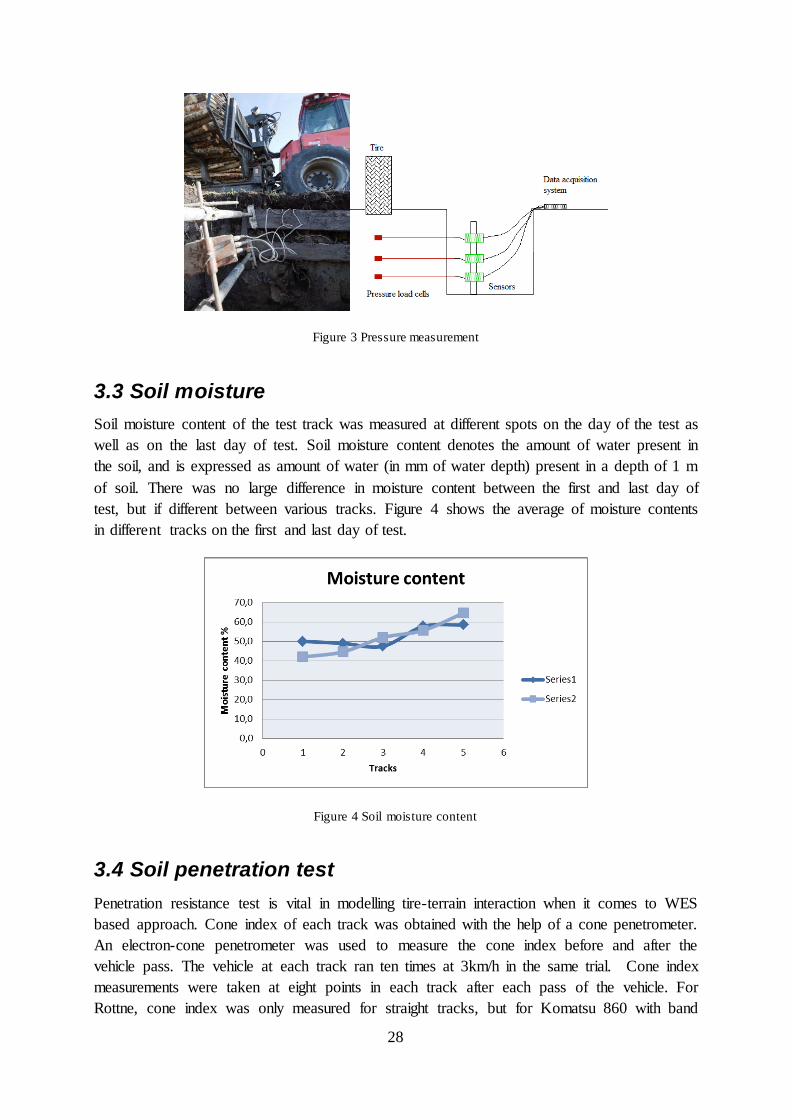
28

Figure 3 Pressure measurement

3.3 Soil moisture

Soil moisture content of the test track was measured at different spots on the day of the test as

well as on the last day of test. Soil moisture content denotes the amount of water present in

the soil, and is expressed as amount of water (in mm of water depth) present in a depth of 1 m

of soil. There was no large difference in moisture content between the first and last day of

test, but if different between various tracks. Figure 4 shows the average of moisture contents

in different tracks on the first and last day of test.

Figure 4 Soil moisture content

3.4 Soil penetration test

Penetration resistance test is vital in modelling tire-terrain interaction when it comes to WES

based approach. Cone index of each track was obtained with the help of a cone penetrometer.

An electron-cone penetrometer was used to measure the cone index before and after the

vehicle pass. The vehicle at each track ran ten times at 3km/h in the same trial. Cone index

measurements were taken at eight points in each track after each pass of the vehicle. For

Rottne, cone index was only measured for straight tracks, but for Komatsu 860 with band

29

tracks, cone index value were measured for S-shaped track also. Cone index measurements

were taken in an interval of 1 cm till 30 cm at each measuring point. The cone index value

measured a 15 cm has the highest predictive power according to Saarilahti (Saarilahti, 2002).

Due to this fact, the cone index value at 15 cm was taken in all the calculations. Figure 5

shows the penetration resistance measured after one vehicle pass of Rottne.

Figure 5 Average values of soil penetration test results at various depths

Figure 6 Soil penetration test after each pass of Rottne

Figure 6 shows the variation of cone index after first, third, fifth and 10th pass of loaded

Rottne. From the diagram, it can be interpreted that the cone index almost remains a constant

when measured in the depth ranging from 5 cm to 20 cm. In each case, the cone index display

an irregular pattern after 20 cm. It is also interesting to note that the cone index after the 3rd

pass is higher when compared to the cone index after the 10th pass.

3.5 Rut depth measurement The rut depths after each vehicle pass were measured at ten points. Rut depths measurements

were taken for both straight and S-shaped tracks. The machine configurations for which rut

depth measurements were taken is given in Table 2. It can be inferred from Figure 7 that, for

an unloaded Rottne, as the number of vehicle passes increases the rut depth also increases.

Also, it has to be noted that the increase in rut depth is not severe as it was for the first three

passes. The rut depth displays an increase when the same machine is under loaded condition.

30

Figure 7 Rut depth measurements for unloaded and loaded conditions of Rottne

Figure 8 shows the rut depth comparison when Rottne maneuvers an S-shaped track. When

the machine is taking an S-shaped track, there is considerable increase in rut depths when

compared to a straight track. It can also be seen that the loaded machine produces more rut

depth.

Figure 8 Rut depth measurements for unloaded and loaded conditions of Rottne in S-curve

3.6 Tire-soil contact area

Tire-soil contact area was measured for two machine configurations. 66 cm x 67 cm, was the

measured area for Komatsu 860 (270 kPa) loaded and 60 cm x 55 cm was for Rottne F13s

(450 kPa).

3.7 Forwarder running gear description

Both, Rottne and Komatsu employed Trelleborg 710/45-26.5 T428 163A8 forestry tire.

Rottne was tested only at 450 kPa tire pressure level, while Komatsu was tested for three tire

pressure levels 270 kPa, 450 kPa and 600 kPa. Table 1 mentions the general forwarder

parameters.

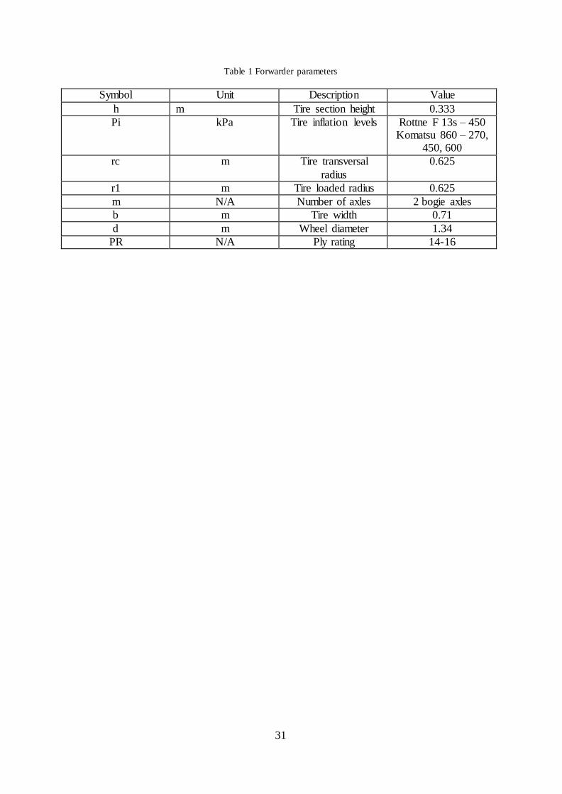
31

Table 1 Forwarder parameters

Symbol Unit Description Value

h m Tire section height 0.333

Pi kPa Tire inflation levels Rottne F 13s – 450 Komatsu 860 – 270,

450, 600

rc m Tire transversal

radius

0.625

r1 m Tire loaded radius 0.625

m N/A Number of axles 2 bogie axles

b m Tire width 0.71

d m Wheel diameter 1.34

PR N/A Ply rating 14-16

32

4 RUT DEPTH ANALYSIS

A detailed study of various rut depth models has been carried out here. New models

developed to predict rut depth’s is also included in this chapter.

4.1 Introduction

The wheel indentations caused by the forest machines while traversing through the terrain is

called ruts. Wheel sinkage is different from rutting; wheel sinkage is measured when the

wheel/vehicle is in static position, while rut depth is measured after the wheel has passed. The

difference between sinkage and rut depths measurement is small (Affleck, July 2005). Rut

depth measurements are one the best indicator to assess the impact of the forest machines on

the forest ground. Rut depths are also caused by wheel slip. Rut depth dimensions are also

affected by steering system as well as transmission systems (Edlund, et al., 2012). The

influence of turning radius on rut depth has also been investigated by Liu, Howard, Anderson,

& Ayers, 2009 (Liu, et al., 2009).

4.2 WES based rut depth models

Most of the WES based rut depth models are for single pass of a wheel. Here, the rut depth

models suggested by Saarilahti (Saarilahti, 2002) are taken into account. Those models are

applied to estimate the rut depth for the single vehicle pass of the forwarder or the rut depth

after the 4th wheel pass. The analysis was done for both Rottne and Komatsu for all the

machine configurations as mentioned in Table 1.

Results of calculations with the available rut depth models to predict the rut depth after the

first vehicle pass was done for both Rottne and Komatsu and is shown in Figure 2Figure 9 and

Figure 10. The equations used for the analysis are presented in the Appendix A3. The

machine configurations tested are described in Table 1.

33

Table 2 Machine configuration

Rottne

Track Machine Condition

1 Rottne Straight Unloaded 450 kPa

2 Rottne Straight Loaded 450 kPa

3 Rottne Loaded Bogie 450 kPa

4 Rottne S track unloaded 450 kPa

5 Rottne S track loaded 450 kPa

6 Rottne straight loaded 450 kPa

Komatsu

Track Machine Condition

1 Komatsu Straight loaded 450 kPa


3 Komatsu Straight unloaded 600 kPa


5 Komatsu S track unloaded 600 kPa

6 Komatsu S track loaded 600 kPa

Figure 9 First vehicle pass rut depth for Rottne

1 2 3 4 5 60

0.02

0.04

0.06

0.08

0.1

0.12

0.14Fourth wheel pass (first vehicle pass) rut depth

For Rottne

Rut

Depth

(m

)

34

Figure 10 First vehicle pass rut depth for Komatsu

For straight track, Antilla 5 and Antilla 7 give good results for Rottne. Antilla 6 and Antilla 7

give good results for Komatsu straight driving condition also. The rut depth models available

cannot be used for rut depth prediction for S shaped tracks; they can only be applied for

straight tracks. In track 4 and 5 for Rottne, which are S shaped (slalom), Antilla model’s 1,2

and 3 give quite satisfactory results. For S shaped tracks, the rut depth calculation has to take

into account the turning radius as well as velocity for accurate prediction; this has been

verified by the works done on military vehicles equipped with tires (Liu, et al., 2009).

Figure 11 Rut depth model description

The equations used in the above mentioned models are derived for specific conditions; they

are not designed to cater the needs of the specific conditions at Tierp. Such empirical

equations can only be applied to conditions in which they were generated or more

specifically, the results given by such equation are more suited to conditions in which they

were developed. The coefficients used in such equations are fitted for the specific conditions,

and the values of such coefficient’s change as the test condition change. It is not

1 2 3 4 5 60

0.02

0.04

0.06

0.08

0.1

0.12

0.14Fourth wheel pass (first vehicle pass) rut depth

For Komatsu

Rut

Depth

(m

)

35

recommended to extrapolate such equations for cases where the test conditions are not in line

with what it was when the equations were developed. In our case, the soil conditions in which

the models were developed were similar, but not exactly. Taking that into account the rut

depth models were used to see, how well it can predicted rutting.

Table 3 WES models description

Antilla 1 Antilla’s (1998) model

Antilla2 Antilla’s (1998) model






Rantala 1 Rantala’s (2001) data for soft soils

Rantala 2 Rantala’s (2001) data for soft soils

Rantala 3 Rantala’s (2001) data for All soils

Saarilahti 1 Saarilahti et. al (1997)

Maclaurin Maclaurin (1990)

GeeGlough Gee-Glough (1985)

4.3 Refinement of WES based rut depth models

The existing WES based models analyzed is not designed for multipass or multiple wheel

pass of vehicles. So the existing models have been fine tuned to take into account the vehicle

pass and also few models have been proposed to take care of the same issue.

4.3.1 Non-linear regression analysis

To make the available models suitable for predicting the rut depth values in Tierp, non-linear

regression analysis was carried out to find suitable coefficients for the models described in

Table 3.By applying the newly derived coefficients to the existing models, the models can be

used for rut depth prediction after the first vehicle pass for the conditions in Tierp. Both the

left side and right side rut depths values of Rottne and Komatsu were used for non-linear

regression analysis to improve the calculation. The new coefficient’s obtained after the non-

linear-regression analysis is shown in Table 4. The results of the non-liner regression analysis

are shown in Figure 12.

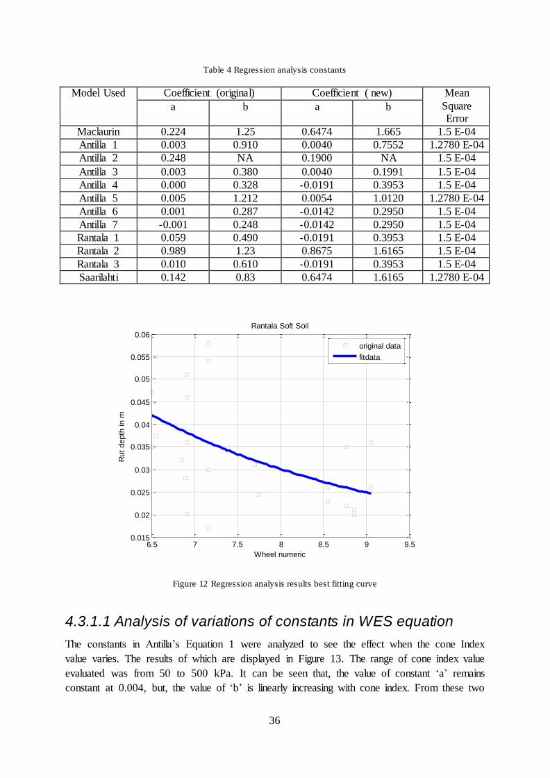
36

Table 4 Regression analysis constants

Model Used

Coefficient (original) Coefficient ( new) Mean

Square Error

a b a b

Maclaurin 0.224 1.25 0.6474 1.665 1.5 E-04

Antilla 1 0.003 0.910 0.0040 0.7552 1.2780 E-04

Antilla 2 0.248 NA 0.1900 NA 1.5 E-04

Antilla 3 0.003 0.380 0.0040 0.1991 1.5 E-04

Antilla 4 0.000 0.328 -0.0191 0.3953 1.5 E-04

Antilla 5 0.005 1.212 0.0054 1.0120 1.2780 E-04

Antilla 6 0.001 0.287 -0.0142 0.2950 1.5 E-04

Antilla 7 -0.001 0.248 -0.0142 0.2950 1.5 E-04

Rantala 1 0.059 0.490 -0.0191 0.3953 1.5 E-04

Rantala 2 0.989 1.23 0.8675 1.6165 1.5 E-04

Rantala 3 0.010 0.610 -0.0191 0.3953 1.5 E-04

Saarilahti 0.142 0.83 0.6474 1.6165 1.2780 E-04

Figure 12 Regression analysis results best fitting curve

4.3.1.1 Analysis of variations of constants in WES equation

The constants in Antilla’s Equation 1 were analyzed to see the effect when the cone Index

value varies. The results of which are displayed in Figure 13. The range of cone index value

evaluated was from 50 to 500 kPa. It can be seen that, the value of constant ‘a’ remains

constant at 0.004, but, the value of ‘b’ is linearly increasing with cone index. From these two

6.5 7 7.5 8 8.5 9 9.50.015

0.02

0.025

0.03

0.035

0.04

0.045

0.05

0.055

0.06

Wheel numeric

Rut

depth

in m

Rantala Soft Soil

original data

fitdata

37

graphs, the conclusion that can be derived is that, the constant ‘b’ is a parameter that depends

on the cone index, which in-turn depends on the soil penetration resistance.

Figure 13 Variation of constants

4.3.2 Application of ‘novel wheel mobility number’

The ‘novel wheel mobility’ number developed by Shawky Hegazy and Corina Sandu (Hegazy

& Sandu, 2013) was introduced in the project to analyze its effect in predicting the rut depth.

The model was applied to Antilla’s equation 3, 4 and 5 replacing NCC, Nci and CN. Non-linear

regression analysis was carried out to find out the new coefficient when ‘novel wheel mobility

number’ was applied. The proposed wheel mobility number is:

HS HS

CIbdN k

W (9)

1

HS

h Rk

d d

(10)

Where,

HSk = proposed coefficient

R1= loaded height of the wheel

h=tire section height

= tire deflection

50 100 150 200 250 300 350 400 450 5000

0.05

0.1

0.15

0.2

0.25

0.3

0.35

Cone index in kPa

Variation o

f consta

nt

a a

nd b

Antillas Equation

constant-b

constant-a

38

Antilla’s equation3, 4 and 5 has been given below respectively.

b

z aN

(11)

Where,

z = rut depth

a,b= constants

N= wheel numeric

Table 5 Antilla’s models original value of constants

a b N

Model 1 0.003 0.380 NCC

Model2 0.000 0.328 NCI

Model3 0.005 01.212 CN

Non-linear regression analysis was carried out to determine the best fitting coefficient for the

Antilla’s equation when the proposed wheel numeric is applied. The new coefficients are

shown in Table 6.

Table 6 New coefficient’s in the Antilla’s model

a b Mean Square Error

Model 1 0.004 0.1991 1.2780 E-04

Model 2 0.0054 0.2668 1.2780 E-04

Model 3 0.0054 0.2668 1.2780 E-04

The new coefficients and the new wheel numeric were applied to Antilla’s equation, rut depth

values were obtained from first vehicle pass for both Komatsu and Rottne, the results of

which are shown in Figure 14 and Figure 15. It can be seen that the results for Komatsu are

satisfactory, especially for the fourth track/machine configuration.

39

Figure 14 Comparison of rut depth with the new model for Rottne

Figure 15 Comparison of rut depth with the new model for Komatsu

The mean square error values of the new equations are similar to the Antilla’s 1 and 5th

model, as well as Saarilahti’s equation, it can be concluded that these models could be used

for estimating the rut depth after the first vehicle pass. It should always be kept in mind that

the equation is empirical and cannot be extrapolated beyond the limits.

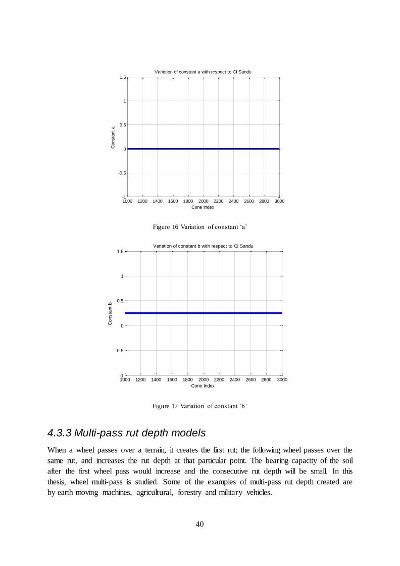
The new wheel mobility number has been applied into Antilla’s equation 5 and variation of

the constants with respect to cone index was studied. It is evident from Figure 16 and Figure

17 that the constants in the equation remain as such for the cone index values ranging from

1000 to 3000 kPa. But, it has been noticed that this value of constants will change for another

range of cone index values. So, it can be inferred that the soil characteristics also have a

bearing on the constants. Further detailed studies are needed to explore the relationships.

1 2 3 4 5 60

0.01

0.02

0.03

0.04

0.05

0.06

For Rottne

Rut

Depth

(m

)

Fourth wheel pass (first vehicle pass) rut depth

Test data

Sandu1

Sandu2

Sandu3

1 2 3 4 5 60

0.01

0.02

0.03

0.04

0.05

0.06

For Komatsu

Rut

Depth

(m

)

Fourth wheel pass (first vehicle pass) rut depth

Test data

Sandu1

Sandu2

Sandu3

40

Figure 16 Variation of constant ‘a’

Figure 17 Variation of constant ‘b’

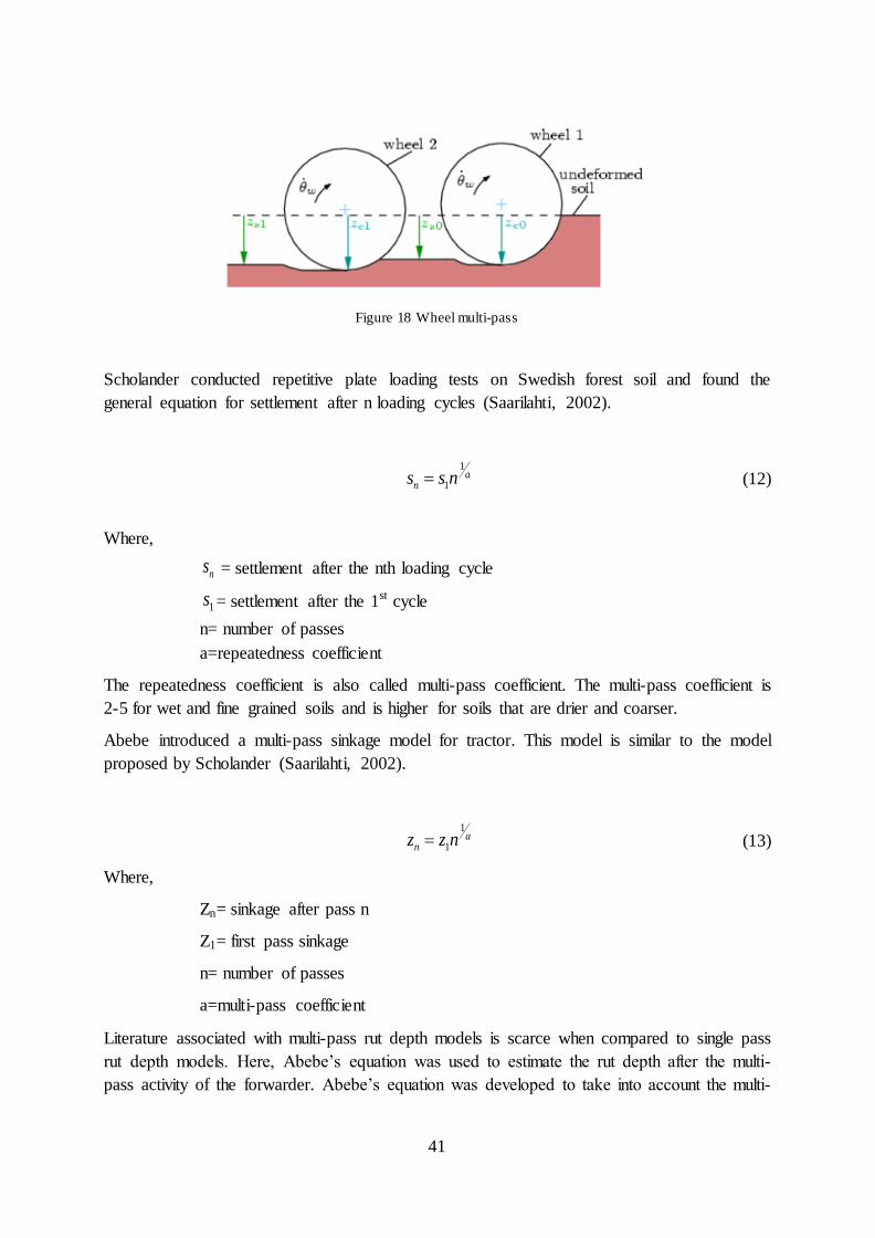
4.3.3 Multi-pass rut depth models

When a wheel passes over a terrain, it creates the first rut; the following wheel passes over the

same rut, and increases the rut depth at that particular point. The bearing capacity of the soil

after the first wheel pass would increase and the consecutive rut depth will be small. In this

thesis, wheel multi-pass is studied. Some of the examples of multi-pass rut depth created are

by earth moving machines, agricultural, forestry and military vehicles.

1000 1200 1400 1600 1800 2000 2200 2400 2600 2800 3000-1

-0.5

0

0.5

1

1.5

Cone Index

Consta

nt

a

Variation of constant a with respect to CI Sandu

1000 1200 1400 1600 1800 2000 2200 2400 2600 2800 3000-1

-0.5

0

0.5

1

1.5

Cone Index

Consta

nt

b

Variation of constant b with respect to CI Sandu

41

Figure 18 Wheel multi-pass

Scholander conducted repetitive plate loading tests on Swedish forest soil and found the

general equation for settlement after n loading cycles (Saarilahti, 2002).

1

1a

ns s n (12)

Where,

ns = settlement after the nth loading cycle

1s = settlement after the 1st cycle

n= number of passes

a=repeatedness coefficient

The repeatedness coefficient is also called multi-pass coefficient. The multi-pass coefficient is

2-5 for wet and fine grained soils and is higher for soils that are drier and coarser.

Abebe introduced a multi-pass sinkage model for tractor. This model is similar to the model

proposed by Scholander (Saarilahti, 2002).

1

1a

nz z n (13)

Where,

Zn= sinkage after pass n

Z1= first pass sinkage

n= number of passes

a=multi-pass coefficient

Literature associated with multi-pass rut depth models is scarce when compared to single pass

rut depth models. Here, Abebe’s equation was used to estimate the rut depth after the multi-

pass activity of the forwarder. Abebe’s equation was developed to take into account the multi-

42

pass effect of a single wheel with a constant load, but in the case at Tierp; the forwarder

wheels had different loads.

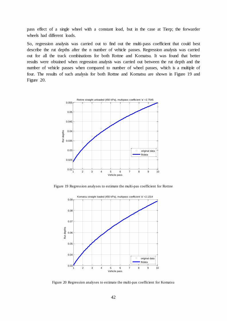
So, regression analysis was carried out to find out the multi-pass coefficient that could best

describe the rut depths after the n number of vehicle passes. Regression analysis was carried

out for all the track combinations for both Rottne and Komatsu. It was found that better

results were obtained when regression analysis was carried out between the rut depth and the

number of vehicle passes when compared to number of wheel passes, which is a multiple of

four. The results of such analysis for both Rottne and Komatsu are shown in Figure 19 and

Figure 20.

Figure 19 Regression analyses to estimate the multi-pas coefficient for Rottne

Figure 20 Regression analyses to estimate the multi-pas coefficient for Komatsu

1 2 3 4 5 6 7 8 9 100.02

0.025

0.03

0.035

0.04

0.045

0.05

0.055

Vehicle pass

Rut

depth

s

Rottne straight unloaded (450 kPa), multipass coefficient 'a' =2.7545

original data

fitdata

1 2 3 4 5 6 7 8 9 100.03

0.04

0.05

0.06

0.07

0.08

0.09

Vehicle pass

Rut

depth

s

Komatsu straight loaded (450 kPa), multipass coefficient 'a' =2.1314

original data

fitdata

43

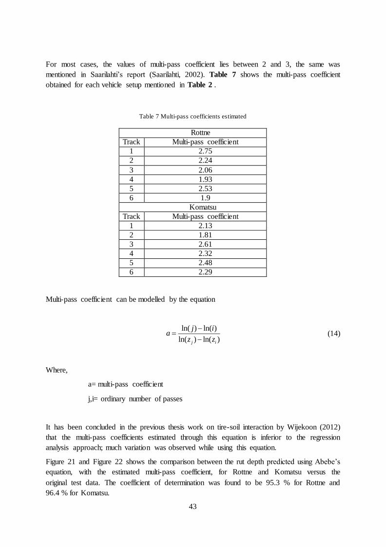
For most cases, the values of multi-pass coefficient lies between 2 and 3, the same was

mentioned in Saarilahti’s report (Saarilahti, 2002). Table 7 shows the multi-pass coefficient

obtained for each vehicle setup mentioned in Table 2 .

Table 7 Multi-pass coefficients estimated

Rottne

Track Multi-pass coefficient

1 2.75

2 2.24

3 2.06

4 1.93

5 2.53

6 1.9

Komatsu

Track Multi-pass coefficient

1 2.13

2 1.81

3 2.61

4 2.32

5 2.48

6 2.29

Multi-pass coefficient can be modelled by the equation

ln( ) ln( )

ln( ) ln( )j i

j ia

z z

(14)

Where,

a= multi-pass coefficient

j,i= ordinary number of passes

It has been concluded in the previous thesis work on tire-soil interaction by Wijekoon (2012)

that the multi-pass coefficients estimated through this equation is inferior to the regression

analysis approach; much variation was observed while using this equation.

Figure 21 and Figure 22 shows the comparison between the rut depth predicted using Abebe’s

equation, with the estimated multi-pass coefficient, for Rottne and Komatsu versus the

original test data. The coefficient of determination was found to be 95.3 % for Rottne and

96.4 % for Komatsu.

44

Figure 21 Predicted rut depth vs. measured rut depth for Rottne

Figure 22 Predicted rut depth vs. measured rut depth for Komatsu

1 2 3 4 5 6 7 8 9 100.02

0.025

0.03

0.035

0.04

0.045

0.05

0.055

Number of vehicle passes

Rut

depth

s (

mete

r)

Rottne Straight unloaded 450 kPa

Test data

Abebe model

1 2 3 4 5 6 7 8 9 100.03

0.04

0.05

0.06

0.07

0.08

0.09


Rut

depth

s (

mete

r)

Komatsu Straight unloaded 450 kPa

Test data

Abebe model

45

4.3.4 Rut depth estimation with changing Cone Index

In most of the models that deal with multi-pass rut depth analysis, the cone index used will be

the one before the vehicle pass or an average cone index value. But, in reality, as each wheel

passes a particular path or point in soil, the soil properties at that specific point changes or the

cone index value varies (Akay, et al., 2006).

In the new model developed, the cone index after each wheel pass has been taken into

account; this new cone index is then used to compute the rut depth caused by the successive

wheels. Maclaurin’s (1990) equation has been used to estimate the sinkage caused by each

wheel.

Brixius has developed an equation to compute the cone index after pass as a function of cone

index before pass and mobility number. This equation is applicable in areas where

compactible soil exists (Akay, et al., 2006).

0.111 1.8 nBACI

eBCI

(15)

51

31

n

CIbd hB

bW

d

(16)

Where,

ACI= cone index after pass

BCI= cone index before pass

Bn= mobility number

= tire deflection

h= tire section height

d= tire diameter

The rut depth created by each wheel was computed by substituting the cone index after each

pass of the previous wheel, so each wheel encounters a new/different terrain, into the

Maclaurin’s equation.

1.25

0.224

CI

z dN

(17)

46

Where,

Z= rut depth

d= wheel diameter

NCI= Wheel numeric

The new method was tried for Rottne, the results of which are shown in Figure 23. Only

straight tracks were considered in the analysis, because, the existing models cannot be used to

estimate the rut depth for S shaped tracks. From Figure 23, it is evident that model can predict

the rut depth well after one vehicle pass, even though not accurate. This model is designed to

take into account the changing soil conditions, which is absent in the other WES based rut

depth models.

Figure 23 Rut depth comparisons with measured data

1 2 3 40

1

2

3

4

5

6

For Rottne

Rut

Depth

(cm

)

1-4 vehcile pass rut depth comparision of Rottne Unloaded (470 kpa tire pressure )

Test data

New method

47

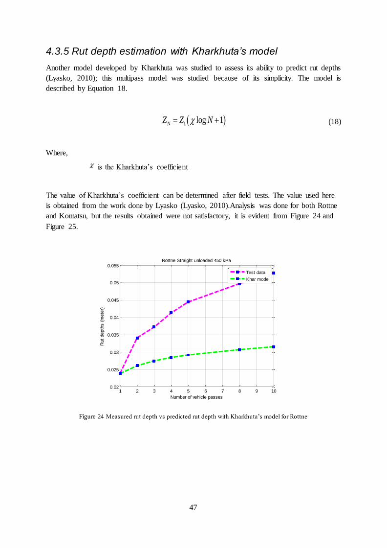
4.3.5 Rut depth estimation with Kharkhuta’s model

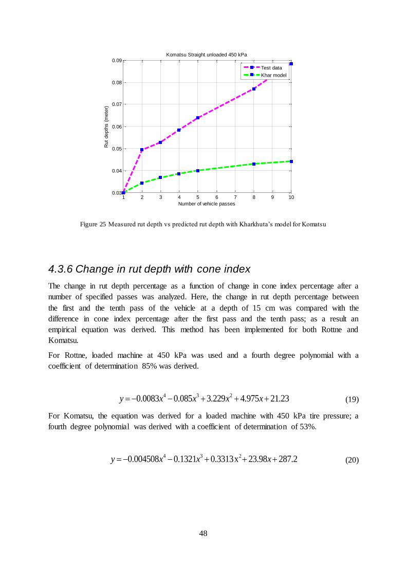
Another model developed by Kharkhuta was studied to assess its ability to predict rut depths

(Lyasko, 2010); this multipass model was studied because of its simplicity. The model is

described by Equation 18.

1 log 1NZ Z N (18)

Where,

is the Kharkhuta’s coefficient

The value of Kharkhuta’s coefficient can be determined after field tests. The value used here

is obtained from the work done by Lyasko (Lyasko, 2010).Analysis was done for both Rottne

and Komatsu, but the results obtained were not satisfactory, it is evident from Figure 24 and

Figure 25.

Figure 24 Measured rut depth vs predicted rut depth with Kharkhuta’s model for Rottne

1 2 3 4 5 6 7 8 9 100.02

0.025

0.03

0.035

0.04

0.045

0.05

0.055


Rut

depth

s (

mete

r)

Rottne Straight unloaded 450 kPa

Test data

Khar model

48

Figure 25 Measured rut depth vs predicted rut depth with Kharkhuta’s model for Komatsu

4.3.6 Change in rut depth with cone index

The change in rut depth percentage as a function of change in cone index percentage after a

number of specified passes was analyzed. Here, the change in rut depth percentage between

the first and the tenth pass of the vehicle at a depth of 15 cm was compared with the

difference in cone index percentage after the first pass and the tenth pass; as a result an

empirical equation was derived. This method has been implemented for both Rottne and

Komatsu.

For Rottne, loaded machine at 450 kPa was used and a fourth degree polynomial with a

coefficient of determination 85% was derived.

4 3 20.0083 0.085 3.229 4.975 21.23y x x x x (19)

For Komatsu, the equation was derived for a loaded machine with 450 kPa tire pressure; a

fourth degree polynomial was derived with a coefficient of determination of 53%.

4 3 20.004508 0.1321 0.3313x 23.98 287.2y x x x (20)

1 2 3 4 5 6 7 8 9 100.03

0.04

0.05

0.06

0.07

0.08

0.09


Rut

depth

s (

mete

r)

Komatsu Straight unloaded 450 kPa

Test data

Khar model

49

Where,

y= change in rut depth percentage

x= change in cone index percentage

The empirical equation so derived can be used to determine the change in rut depth

percentage for the specific vehicles in the specific soil terrain at Tierp. More filed test needs

to be done to determine the effectiveness of the equation.

4.3.7 Cone Index vs. Depth of measurement

In this section, the cone index variation at various depths of measurement after specific

number of vehicle passes was analyzed. Empirical equations were derived for the evaluation

of cone index at different depth, till 21 cm, after specific vehicle passes. Figure 26 show the

variation of cone index with depth for Rottne and ProSilva.

Figure 26 Variation of cone index with depth after specific number of vehicle passages

0

5

10

15

20

250.2 0.4 0.6 0.8 1 1.2 1.4 1.6

Depth

of

measure

ment

in c

m

Cone index measurement in mPa

Rottne Loaded 450 kPa

After 1st pass

After 5th pass

After 10th pass

0

5

10

15

20

250 0.2 0.4 0.6 0.8 1 1.2 1.4

Depth

of

measure

ment

in c

m


ProSilva Loaded

After 1st pass

After 5th pass

After 10th pass

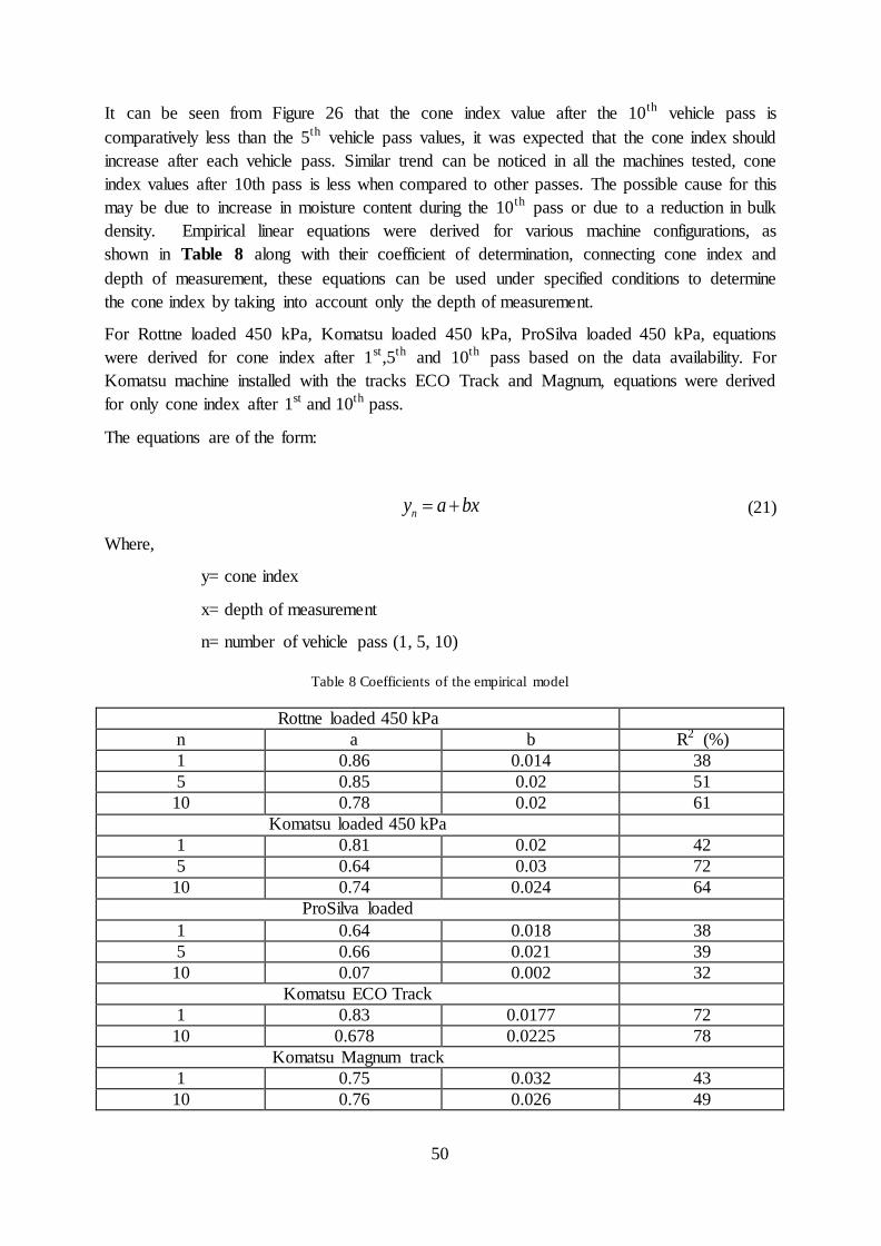
50

It can be seen from Figure 26 that the cone index value after the 10th vehicle pass is

comparatively less than the 5th vehicle pass values, it was expected that the cone index should

increase after each vehicle pass. Similar trend can be noticed in all the machines tested, cone

index values after 10th pass is less when compared to other passes. The possible cause for this

may be due to increase in moisture content during the 10th pass or due to a reduction in bulk

density. Empirical linear equations were derived for various machine configurations, as

shown in Table 8 along with their coefficient of determination, connecting cone index and

depth of measurement, these equations can be used under specified conditions to determine

the cone index by taking into account only the depth of measurement.

For Rottne loaded 450 kPa, Komatsu loaded 450 kPa, ProSilva loaded 450 kPa, equations

were derived for cone index after 1st,5th and 10th pass based on the data availability. For

Komatsu machine installed with the tracks ECO Track and Magnum, equations were derived

for only cone index after 1st and 10th pass.

The equations are of the form:

ny a bx (21)

Where,

y= cone index

x= depth of measurement

n= number of vehicle pass (1, 5, 10)

Table 8 Coefficients of the empirical model

Rottne loaded 450 kPa

n a b R2 (%)

1 0.86 0.014 38

5 0.85 0.02 51

10 0.78 0.02 61

Komatsu loaded 450 kPa

1 0.81 0.02 42

5 0.64 0.03 72

10 0.74 0.024 64

ProSilva loaded

1 0.64 0.018 38

5 0.66 0.021 39

10 0.07 0.002 32

Komatsu ECO Track

1 0.83 0.0177 72

10 0.678 0.0225 78

Komatsu Magnum track

1 0.75 0.032 43

10 0.76 0.026 49

51

It can be seen from Table 8, coefficient a, ranges from 0.6 to 0.9 and the coefficient b ranges

from 0.01 to 0.03. This range represents a trend; results from more field test can be used to

estimate the stability of this range. From Figure 26, it can be seen that the graph does not look

linear; but linear equations were proposed to keep the analysis simple and to reduce the

number of coefficients. A word of caution, more tests needs to be done to fix the suitability

of the equation, various machine configurations has to be tested under various conditions so

as to generalize and suggest a range of values for the coefficients in the equation.

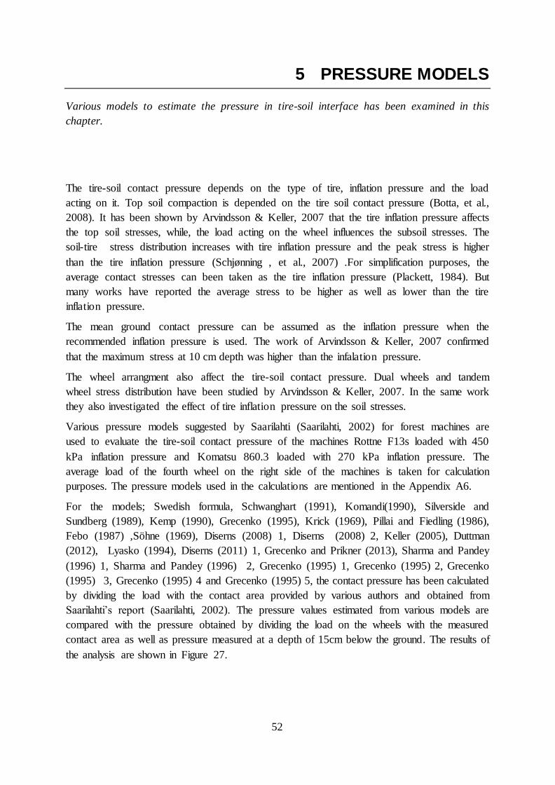
52

5 PRESSURE MODELS

Various models to estimate the pressure in tire-soil interface has been examined in this

chapter.

The tire-soil contact pressure depends on the type of tire, inflation pressure and the load

acting on it. Top soil compaction is depended on the tire soil contact pressure (Botta, et al.,

2008). It has been shown by Arvindsson & Keller, 2007 that the tire inflation pressure affects

the top soil stresses, while, the load acting on the wheel influences the subsoil stresses. The

soil-tire stress distribution increases with tire inflation pressure and the peak stress is higher

than the tire inflation pressure (Schjønning , et al., 2007) .For simplification purposes, the

average contact stresses can been taken as the tire inflation pressure (Plackett, 1984). But

many works have reported the average stress to be higher as well as lower than the tire

inflation pressure.

The mean ground contact pressure can be assumed as the inflation pressure when the

recommended inflation pressure is used. The work of Arvindsson & Keller, 2007 confirmed

that the maximum stress at 10 cm depth was higher than the infalation pressure.

The wheel arrangment also affect the tire-soil contact pressure. Dual wheels and tandem

wheel stress distribution have been studied by Arvindsson & Keller, 2007. In the same work

they also investigated the effect of tire inflation pressure on the soil stresses.

Various pressure models suggested by Saarilahti (Saarilahti, 2002) for forest machines are

used to evaluate the tire-soil contact pressure of the machines Rottne F13s loaded with 450

kPa inflation pressure and Komatsu 860.3 loaded with 270 kPa inflation pressure. The

average load of the fourth wheel on the right side of the machines is taken for calculation

purposes. The pressure models used in the calculations are mentioned in the Appendix A6.

For the models; Swedish formula, Schwanghart (1991), Komandi(1990), Silverside and

Sundberg (1989), Kemp (1990), Grecenko (1995), Krick (1969), Pillai and Fiedling (1986),

Febo (1987) ,Söhne (1969), Diserns (2008) 1, Diserns (2008) 2, Keller (2005), Duttman

(2012), Lyasko (1994), Diserns (2011) 1, Grecenko and Prikner (2013), Sharma and Pandey

(1996) 1, Sharma and Pandey (1996) 2, Grecenko (1995) 1, Grecenko (1995) 2, Grecenko

(1995) 3, Grecenko (1995) 4 and Grecenko (1995) 5, the contact pressure has been calculated

by dividing the load with the contact area provided by various authors and obtained from

Saarilahti’s report (Saarilahti, 2002). The pressure values estimated from various models are

compared with the pressure obtained by dividing the load on the wheels with the measured

contact area as well as pressure measured at a depth of 15cm below the ground. The results of

the analysis are shown in Figure 27.

53

Figure 27 Tire-soil contact pressure comparisons for Rottne and Komatsu

All the models provide the pressure at the contact surface between the tire and the soil, so it

seemed feasible to compare the pressure values obtained from various models with the

pressure obtained by dividing the load by contact area. It is evident from the plots that most of

the models do not predict the exact value, that is, the one obtained by dividing wheel load by

contact area. It has to be noticed that the pressure obtained by dividing the load with the

contact area is a simplified process, in reality, the soil pressure under a deformed tire is not

uniform.

In case of Rottne, only, Schwanghart (1991) model ( Schwanghart, 1991) is near to the

pressure measured. For Komatsu, models like, MMP Moist clay 1, MMP Moist clay 2,

Disern’s (2008) 1, Disern’s 2008 (2) (Diserns, 2008) and Duttmann (2012) (Duttmann, et al.,

2012) provide values that are similar to the one obtained by obtained by dividing the load by

contact area. As it is hard to estimate the exact value of the ground pressure due to the

complex interaction between the soil and the tire, the models whose results are almost similar

can be taken into account. Also, these models proposed here, can be taken to compare the tire-

contact pressure of various machines or machine configurations.

But, from Table 9, it can be seen that the pressure at a depth of 15 cm is 255 kPa for Rottne

and 133 kPa for Komatsu. The pressure at the contact surface between the tire and soil will

definitely be more than 255 kPa and 133 kPa. Therefore, all the models that provide a value

around 255 kPa can be considered. So, if the pressure at 15 cm depth is taken a yardstick to

evaluate the pressure exerted by the tire, then for Rottne, only the model Per (2010) gives

realistic result. But for Komatsu, Ground pressure index, Empirical, Keller (2005) and

Disern’s (2011) 2 gives nearby results. It has to be noted again that, these models are created

for determining the surface pressure, even though they are considered for pressure estimation

at 15 cm depth.

54

Table 9 Pressure values obtained from different models

Pressure models in kPa

Model Rottne Komatsu

1 Measured at 15 cm 255 133

2 Measured with contact area 141,2121 113,071

3 MMP Moist clay 1 104,1581 96,01613

4 MMP Moist clay 2 102,7476 110,2442

5 MMP Moist clay 3 89,19849 95,70653

6 Koolen (1992) 900 540

7 Boling (1985) 490 310

8 Steiner (1979) 431,618 314,91

9 NGP 57,4112 61,6

10 Dwyer (1984) 343,6524 316,7892

11 Ground pressure index 160,5798 152,5909

12 Pneumatic tire on hard surface 1 281,4245 226,5614



15 Swedish formula 76,86844 82,47686

16 Schwanghart (1990) 149,4342 140,6362

17 Empirical 189 131,4

18 Komandi (1990) 210,575 170,9031

19 Silverside and Sundberg (1989) 500 300

20 Kemp (1990) 450 450

21 Grecenko (1995) 184,342 197,7919

22 Krick (1969) 1 410,4923 325,1046

23 Krick (1969) 2 295,7585 372,9079

24 Pillai and Fiedling (1986) 313,6166 274,8352

25 Febo (1987) 170,1039 143,1681

26 Ziesak and Matthies (2001) 503,8587 416,2172

27 Söhne (1969) 169,4433 168,2188

28 Diserns (2008) 1 108,6815 110,8198

29 Diserns (2008) 2 103,0062 105,2105

30 Keller (2005) 173,0065 129,009

31 Duttmann (2012) 114,0139 111,7596

32 Lyasko (1994) 574,9605 411,5294

33 Diserns (2011) 1 183,518 196,9078

34 Diserns (2011) 2 134,6512 144,4756

35 Per (2010) 267,8 170,6

36 Grecenko (2014) 121,8328 130,7219

37 Sharma and Pandey (1996) 1 409,2652 324,1327

38 Sharma and Pandey (1996) 2 521,0926 412,6985

39 Grecenko (1995) 1 184,342 197,7919

40 Grecenko (1995) 2 324,6729 348,3614

41 Grecenko (1995) 3 295,1805 316,7172

42 Grecenko (1995) 4 400,1726 283,6072

43 Rodriguez et al (2012) 346,14 262,6

55

The Nominal Ground Pressure model is based on the assumption of fifteen percent sinkage

(Saarilahti, 2002). The model is considered as a standard that is used in Nordic forest

research. As expected this model gives very low ground pressure values when compared to

other models. But the model is used an indicator of trafficability for wheeled as well as

tracked vehicles (Saarilahti, 2002).

It can be seen from the work of Hetherington & White, (2002) that the MMP models do not

represent actual ground pressure. It can work as an indicator of vehicle performance rather

than a model to predict the actual contact pressure.

The model proposed by Komandi (1990) was developed for agricultural tires (Saarilahti,

2002). In the model proposed by Silverside and Sundberg (1989), it is assumed that ten

percent wheel load is supported by side walls.

Whereas, Kemp (1990) assumed the sidewall support to be zero and proposed the inflation

pressure to be equal to the ground pressure. Febo (1987) used wide agricultural tires to

suggest the pressure model that is applicable to hard surface; the values predicted by Febo

(1987) were very high.

The values predicted by Ziesak and Matthies (2001) were within a good range of the original

values, Ziesak and Matthies (2001) model were developed to predict average contact pressure

for forestry tires on hard surface. The model by Lyasko (Lyasko, 1994) gives good results; the

model is based on a tests on rigid surface conducted with the help of a single-wheel tester.

Diseren’s (2008) model gives good results, this empirical model have been developed by

testing twenty four different trailer tires, both cross-ply and radial were taken into account, in

soils ranging from soft to hard.

The model proposed by Keller (2005) (Keller, 2005), is based on field experiments with

tractors , trailers and harvesters in Sweden and Denmark for agricultural tires, this model also

provide a good estimate of the contact pressure. The model given by Duttmann, et al., 2012

also provides results that are comparable, the eqution is based on field study conducted in

clayey silt soil in German farm vehicles.

Diserens , et al., (2011) model was developed for traction tires for grasslands and open ground

sites, harvesters and tractors were used for the experiment, the model provided good results.

The model proposed by Per (2010) , predicted contact pressure with the help of tests done

with radial tires in Sandy soil, even though the test conditions and tire type was different from

what it was on the tested forwarders at Tierp, the model provided satisfactory results.

The contact area value for a rectangular patch provided by Sharma and Pandey (Sharma &

Pandey, 1996) were used to obtain the contact pressure, the result was satisfactory when the

contact area was used for a rectangular patch, but in reality, the conatct patch is not exactly

rectangular, an elliptical patch provides a better estimate of the contact area (Wulfsohn &

Upadhyaya, 1992). Grecenko’s (1995) model (Grecenko, 1995), has been created for hard

grounds, it returns satisfactory value of contact pressure in the calculations.

56

The work of Cirello, et al., (2009) show that the ground surface pressure will be in the range

of 200 to 600 kPa, and that too for a tire with load ranging from 4 kN to 6 kN. From this

result, it can be observed that all the models that provide a pressure value less than 200 kPa

seems less realistic, but, this work was carried out for hard surface, so a complete rejection of

the all the models that return values less that 200 kPa cannot be done unless or until an

expiremtal analysis has been carried out similar to what Cirello, et al., (2009) has been done

in soft soil.

Another interesting observation is that, the work done by Lamande´ & Schjønning, (2011)

suggests a maximum surface pressure of 200 kPa for a 60 kN loaded wheel. Therefore, a

model than can accurately predict the surface pressure is lacking. But experimental method

followed by Cirello, et al., (2009) seems to be a good option to find accurate pressure, this

approach can be used further to develop an empirical model.

Hetherington & White (2002), from their studies have shown that the surface pressure can be

found by using a multipying factor with the pressure measured at a specified depth. But the

uncertanity existing over such a factor acts a major source of error in determing the surface

pressure.

The surface pressure value also depend on the type of soil, tyre inflation pressure and vehicle

weight. Higher weight and higher inflation pressure would increase in the ground pressure

level.

It has been mentioned by Wästerlund (Wästerlund, 1989), that trees standing near to the ruts

whose soil layer is exposed to contact pressure of 60-90 kPa show reduced growth. Also

spruce seedling demonstrates reduced growth when exposed to static load greater than 80 kPa.

It is evident from the analysis above that the machines analyzed apply contact pressure greater

that the threshold values mentioned by Wästerlund, this highlights the impact the machines

can have on the forest floor.

57

6 Tire-Soil Contact Area

This chapter provides an insight into various models that are used to determine the contact -

patch area between a tire and soil.

Tire soil contact area is a very important parameter in determining various aspects of vehicle

mobility. The loaded area play an important role in determining the distribution of stresses at

the soil surface, and also affects the stress in subsoil. The stresses in soil are directly

dependent on stresses on the tire soil interface. To determine the stresses in the soil, the

contact area has to be estimated accurately and the performance of soil compaction models

are highly dependent on the contact area (Keller, 2005). So, accurate estimation of the tire-soil

contact area play a prominent role in improving the stress propogation models.

The precise determination of contact area is necessary in the finite element analysis of tire-

soil interaction (Yong, et al., 1984). Contact area comes into picture when determing the

surface pressures (Döll, 2001) as well as when estimating the soil compaction (Defossez &

Richard, 2002) .

The contact area depends on factors like plasticity and elsticity of both tire and ground. It has

been mentioned by Diserns, et al., 2011 about the dependence of the contact area in farmlands

on the forces acting on the wheels, namely, traction force, bracking force and rolling

resistance. As the surface gets harder, for a given load and inflation pressure, the contact area

increases (Diserns, 2008). For bigger tires, the contact area increase with the wheel load.

The tire inflation pressure influences the tire foot-print area as can be seen from the work of

Schjønning , et al., 2007. The contact area doubles when reducing the inflation pressure. If the

recommeded inflation pressure is used, then the contact area will be an intermediate value

(Schjønning , et al., 2007).

The contact area between a pneumatic tire and a hard surface can be considered as a circle, if

the tire has high inflation pressure and if it is of cross-ply type. As the tire pressure reduces

the contact area transforms to an elliptical shape, similar shape can be seen on softer ground

also.

Various models associated with calculating the contact area the tire soil interface has been

done, the models are described in Appendix A5. The tire-soil contact area estimation has been

done for Rottne F13s loaded with 450 kPa inflation pressure and Komatsu 860 loaded with

270 kPa inflation pressure as the measured tire-soil contact imprint area is only available for

them. The results of the estimated contacted area with different models is shown in Figure 28.

The model, Per Schjønning (2007), is not applicable to Komatsu; being an empirical model it

does not satisfy the conditions under which Komatsu was tested.

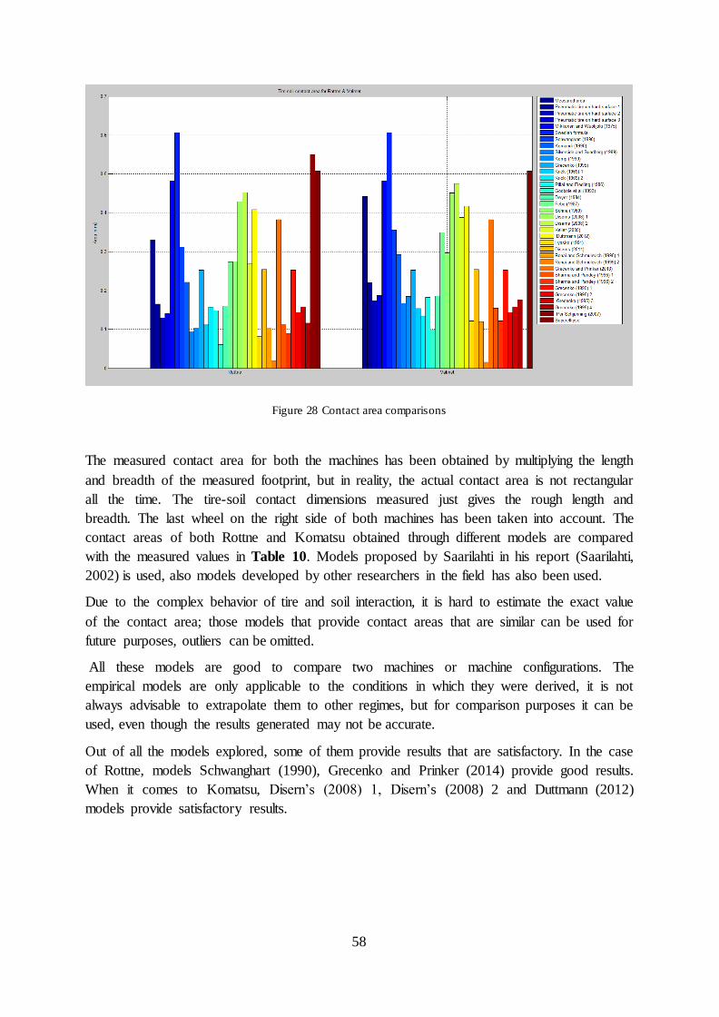
58

Figure 28 Contact area comparisons

The measured contact area for both the machines has been obtained by multiplying the length

and breadth of the measured footprint, but in reality, the actual contact area is not rectangular

all the time. The tire-soil contact dimensions measured just gives the rough length and

breadth. The last wheel on the right side of both machines has been taken into account. The

contact areas of both Rottne and Komatsu obtained through different models are compared

with the measured values in Table 10. Models proposed by Saarilahti in his report (Saarilahti,

2002) is used, also models developed by other researchers in the field has also been used.

Due to the complex behavior of tire and soil interaction, it is hard to estimate the exact value

of the contact area; those models that provide contact areas that are similar can be used for

future purposes, outliers can be omitted.

All these models are good to compare two machines or machine configurations. The

empirical models are only applicable to the conditions in which they were derived, it is not

always advisable to extrapolate them to other regimes, but for comparison purposes it can be

used, even though the results generated may not be accurate.

Out of all the models explored, some of them provide results that are satisfactory. In the case

of Rottne, models Schwanghart (1990), Grecenko and Prinker (2014) provide good results.

When it comes to Komatsu, Disern’s (2008) 1, Disern’s (2008) 2 and Duttmann (2012)

models provide satisfactory results.

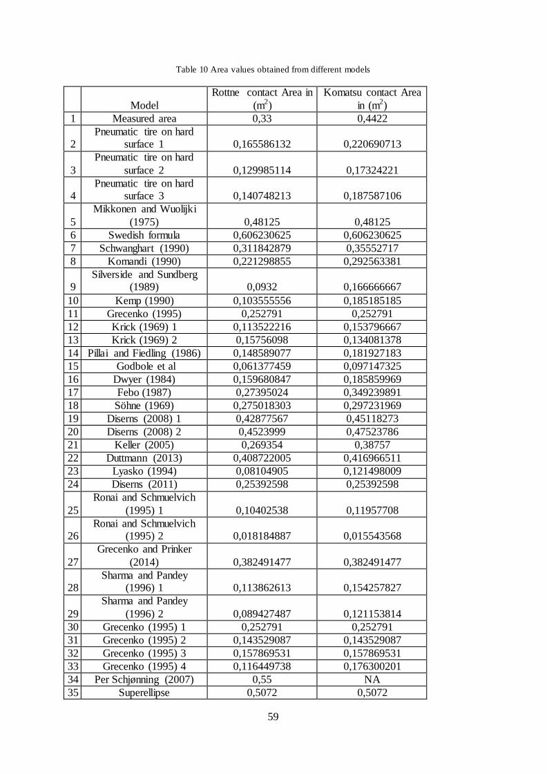
59

Table 10 Area values obtained from different models

Model

Rottne contact Area in

(m2)

Komatsu contact Area

in (m2)

1 Measured area 0,33 0,4422

2 Pneumatic tire on hard

surface 1 0,165586132 0,220690713

3

Pneumatic tire on hard

surface 2 0,129985114 0,17324221

4 Pneumatic tire on hard

surface 3 0,140748213 0,187587106

5

Mikkonen and Wuolijki

(1975) 0,48125 0,48125

6 Swedish formula 0,606230625 0,606230625

7 Schwanghart (1990) 0,311842879 0,35552717

8 Komandi (1990) 0,221298855 0,292563381

9 Silverside and Sundberg

(1989) 0,0932 0,166666667

10 Kemp (1990) 0,103555556 0,185185185

11 Grecenko (1995) 0,252791 0,252791

12 Krick (1969) 1 0,113522216 0,153796667

13 Krick (1969) 2 0,15756098 0,134081378

14 Pillai and Fiedling (1986) 0,148589077 0,181927183

15 Godbole et al 0,061377459 0,097147325

16 Dwyer (1984) 0,159680847 0,185859969

17 Febo (1987) 0,27395024 0,349239891

18 Söhne (1969) 0,275018303 0,297231969

19 Diserns (2008) 1 0,42877567 0,45118273

20 Diserns (2008) 2 0,4523999 0,47523786

21 Keller (2005) 0,269354 0,38757

22 Duttmann (2013) 0,408722005 0,416966511

23 Lyasko (1994) 0,08104905 0,121498009

24 Diserns (2011) 0,25392598 0,25392598

25

Ronai and Schmuelvich

(1995) 1 0,10402538 0,11957708

26 Ronai and Schmuelvich

(1995) 2 0,018184887 0,015543568

27

Grecenko and Prinker

(2014) 0,382491477 0,382491477

28 Sharma and Pandey

(1996) 1 0,113862613 0,154257827

29

Sharma and Pandey

(1996) 2 0,089427487 0,121153814

30 Grecenko (1995) 1 0,252791 0,252791

31 Grecenko (1995) 2 0,143529087 0,143529087

32 Grecenko (1995) 3 0,157869531 0,157869531

33 Grecenko (1995) 4 0,116449738 0,176300201

34 Per Schjønning (2007) 0,55 NA

35 Superellipse 0,5072 0,5072

60

The Schwanghart (1991) model ( Schwanghart, 1991) is based on tests done with four

different tires at different inflation pressure and different loads in a soil bin filled with sandy

loam, the results are more close to area measured in Rottne, the variations are due to the

inherent empirical modelling characteristics.

The area predicted by Grecenko and Prikner (2013) model (Grecenko & Prikner, 2013) is

comparatively away from the original area than Schwanghart model. Here, pressure plates in

soil containers were used for testing compaction capacity of soil, Suchdol loam was used in

the test.

The Disern’s (2008) model (Diserns, 2008) is based on test done on soft to hard soils with

trailer tires, by applying various loads and inflation pressures. The tires that were taken into

account include Cross-ply farming tires, Radial low size tires and Radial terra tires. This work

is more reliable in semi-firm to firm soil types.

The Duttmann (2012) model (Duttmann, et al., 2012) is based on test carried out during silage

maize harvest in Germany during the Autumn of 2008. The soil type was mainly clayey silt

and machines tested include a Forage harvester, a tractor and a trailer (tandem axle).

6.1 Super ellipse as tire soil contact area

If the tire pressure is low or the softer the ground, the shape of the contact area is elliptical

(Hallonborg, 1996). For vehicles traversing in forestry terrain the contact area is not

symmetric about its transverse axis. In such cases, each quadrant of the elliptical contact area

produces different shapes or its own elliptical shape. Mathematical equations for deriving the

contact areas in such cases are intricate. The approach of modelling the tire soil contact area

as super ellipse was introduced by Hallonborg, 1996. The equation of the super ellipse in

orthogonal coordinate system is:

1n n

n n

x y

a b (22)

where: n determine the shape of the ellipse, a and b are the half axes of the super ellipse.

When n =2, the curve is an ellipse. For n=2, when a=b, the curve becomes a circle. The curve

changes to a rectangle lying on a side as n tends to (Hallonborg, 1996).

The tire soil contact area can be obtained by taking the sum of the areas in each of the four

quadrants; the area of one quadrant is given by:

1

0

1

a n n

quadrant n

xA b dx

a

(23)

61

2

2.10 2tyre tyren w d (24)

Where,

a = tyrew =tire width in m

b = length of contact area in m

tyred = tire diameter in m

Figure 29 Superellipse as tire-soil contact area

Super ellipse concept was used to obtain the tire-soil contact area of both the forwarders, the

results of which is mentioned in Table 10 and shown in Figure 29. From the works of

Hallonborg, 1996 and Keller, 2005, the super ellipse model can be considered to provide an

accurate and reliable estimate of the conatct area. Super ellipse model has been tested many

times and is accepted as a model that gives accurate values for various tires; it is evident from

the test carried out by Schjønning , et al., 2007. So, the super ellipse model can be considered

to be more relaibale than the other models.

-0.4 -0.3 -0.2 -0.1 0 0.1 0.2 0.3 0.4-0.4

-0.3

-0.2

-0.1

0

0.1

0.2

0.3

0.4

Breadth (m)

Length

(m

)

Superellipse as tyre-contact area

62

7 Mobility Models

Mobility models are scrutinized here in order to get an overall idea about their feasibility.

The mobility models or mobility parameters can be used to assess the vehicle mobility. There

are different mobility models proposed by different authors. The mobility numbers

investigated in this project include, thrust coefficient, rolling resistance coefficient and

drawbar pull coefficient. These variables could give an idea about the performance of the

vehicle in a specific terrain.

Thrust coefficient gives an idea about gross traction, drawbar pull deals with net traction and

finally rolling resistance coefficient gives a picture about the resistance encountered by the

wheels of the vehicle.

Different models dealing with mobility number estimation are available; the models used in

the project include the ones suggested by Saarilahti (Saarilahti, 2002). The models used

include Turnage(WESFIELD), Turnage(WESLAB), Wismer&Luth, N.I.A.E models, Brixius,

Ashmore et al.,Rummer and Ashmore, Maclaurin, Sharma and Pandey, McAllister and finally

the model suggested by Bruce Maclaurin (Maclaurin, 2013). The equations used are attached

in Appendix A4. The calculation is based on the average loads on the front wheels. The

results of the analysis are shown in Table 11.

Table 11 Mobility parameters for Rottne

Rottne straight loaded 450 kPa

Mobility Models P R T

Turnage (1972b), WESFIELD 0,081637 0,152766 NA

Turnage (1972a), WESLAB 0,298868 0,112109 NA

Wismer and Luth (1973) 0,211762 0,149543 0,361305

N.I.A.E Models 0,450022 0,924718 NA

Brixiuis (1987) 0,111106 0,186453 0,333558

Ashmore et al (1987) 0,633281 0,034753 NA

Rummer and Ashmore (1985) NA 0,228545 NA

Maclaurin (1990) 0,282501 0,123 NA

Maclaurin (1990_rounded wheel

numeric/new)

0,263134 0,128837 NA

Sharma and Pandey (1998) 0,055395 NA 0,113417

McAllister NA 0,12958 NA

Bruce Maclaurin (2013) NA 0,139589 NA

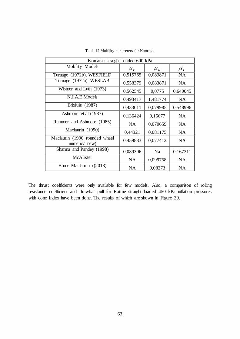
63

Table 12 Mobility parameters for Komatsu

Komatsu straight loaded 600 kPa

Mobility Models P R T

Turnage (1972b), WESFIELD 0,515765 0,083871 NA

Turnage (1972a), WESLAB 0,558379 0,083871 NA

Wismer and Luth (1973) 0,562545 0,0775 0,640045

N.I.A.E Models 0,493417 1,481774 NA

Brixiuis (1987) 0,433011 0,079985 0,548996

Ashmore et al (1987) 0,136424 0,16677 NA

Rummer and Ashmore (1985) NA 0,070659 NA

Maclaurin (1990) 0,44321 0,081175 NA

Maclaurin (1990_rounded wheel numeric/ new)

0,459883 0,077412 NA

Sharma and Pandey (1998) 0,089306 Na 0,167311

McAllister NA 0,099758 NA

Bruce Maclaurin ((2013) NA 0,08273 NA

The thrust coefficients were only available for few models. Also, a comparison of rolling

resistance coefficient and drawbar pull for Rottne straight loaded 450 kPa inflation pressures

with cone Index have been done. The results of which are shown in Figure 30.

64

Figure 30 Evaluation of rolling resistance coefficient and pull coefficient with changing cone index

It is evident from the figure that drawbar pull coefficient increases as the cone index increases

and from the figure it can be inferred that the rolling resistance coefficient decreases as cone

index increases.

The range of cone index that was used for calculation was from 940 kPa to 1200 kPa, all the

models gave good results in this range. For rolling resistance coefficient, Brixius, Turnage

900 950 1000 1050 1100 1150 12000

0.5

1

1.5

2

2.5

CONE INDEX (kPa)

Rolli

ng R

esis

tance C

oeff

icie

nt

CONE INDEX vs. ROLLING RESISTANCE COEFFICIENT of Rottne Straight loaded 450 kPa

Turnage WESFIELD

Turnage WESLAB

Wismer and Luth

N.I.A.E models

Brixius

Ashmore et al

Rummer and Ashmore

Maclaurin

Mclaurin-New

McAllister

Bruce Maclaurin (2013)

900 950 1000 1050 1100 1150 12000.1

0.2

0.3

0.4

0.5

0.6

0.7

0.8

CONE INDEX (kPa)

Pull

coeff

cie

nt

CONE INDEX vs. PULL COEFFCIENT of Rottne Straight loaded 450 kPa

Turnage WESLAB

Wismer and Luth

N.I.A.E Models

Brixius

Ashmore et al

Maclaurin

Maclaurin-new

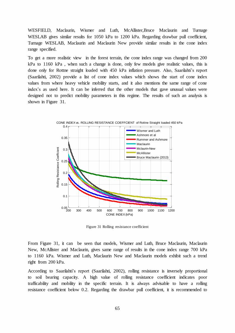
65

WESFIELD, Maclaurin, Wismer and Luth, McAllister,Bruce Maclaurin and Turnage

WESLAB gives similar results for 1050 kPa to 1200 kPa. Regarding drawbar pull coefficient,

Turnage WESLAB, Maclaurin and Maclaurin New provide similar results in the cone index

range specified.

To get a more realistic view in the forest terrain, the cone index range was changed from 200

kPa to 1160 kPa , when such a change is done, only few models give realistic values, this is

done only for Rottne straight loaded with 450 kPa inflation pressure. Also, Saarilahti’s report

(Saarilahti, 2002) provide a list of cone index values which shows the start of cone index

values from where heavy vehicle mobility starts, and it also mentions the same range of cone

index’s as used here. It can be inferred that the other models that gave unusual values were

designed not to predict mobility parameters in this regime. The results of such an analysis is

shown in Figure 31.

Figure 31 Rolling resistance coefficient

From Figure 31, it can be seen that models, Wismer and Luth, Bruce Maclaurin, Maclaurin

New, McAllister and Maclaurin, gives same range of results in the cone index range 700 kPa

to 1160 kPa. Wismer and Luth, Maclaurin New and Maclaurin models exhibit such a trend

right from 200 kPa.

According to Saarilahti’s report (Saarilahti, 2002), rolling resistance is inversely proportional

to soil bearing capacity. A high value of rolling resistance coefficient indicates poor

trafficability and mobility in the specific terrain. It is always advisable to have a rolling

resistance coefficient below 0.2. Regarding the drawbar pull coefficient, it is recommended to

200 300 400 500 600 700 800 900 1000 1100 12000.05

0.1

0.15

0.2

0.25

0.3

0.35

0.4

CONE INDEX (kPa)

Rolli

ng R

esis

tance C

oeff

cie

nt

CONE INDEX vs. ROLLING RESISTANCE COEFFCIENT of Rottne Straight loaded 450 kPa

Wismer and Luth

Ashmore et al

Rummer and Ashmore

Maclaurin

Mclaurin-New

McAllister


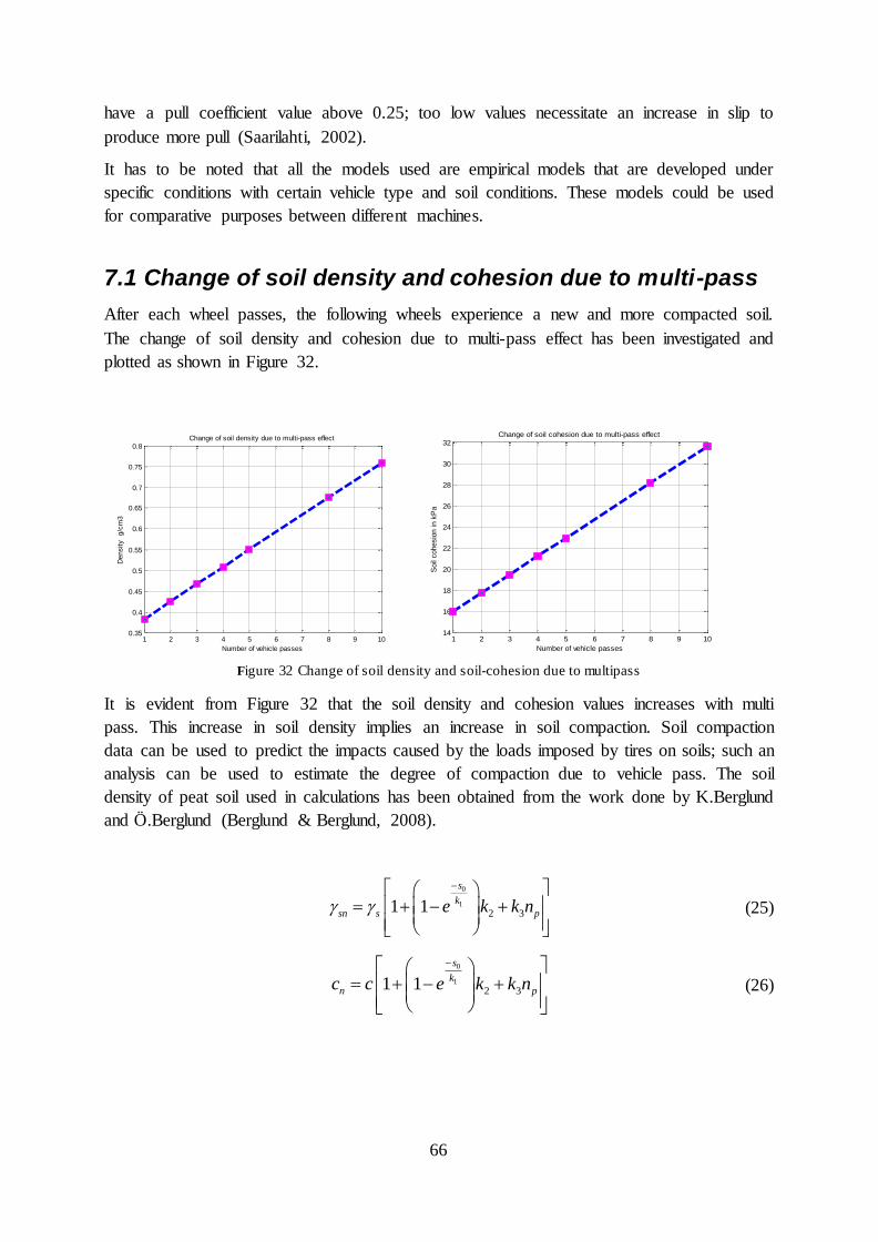
66

have a pull coefficient value above 0.25; too low values necessitate an increase in slip to

produce more pull (Saarilahti, 2002).

It has to be noted that all the models used are empirical models that are developed under

specific conditions with certain vehicle type and soil conditions. These models could be used

for comparative purposes between different machines.

7.1 Change of soil density and cohesion due to multi-pass

After each wheel passes, the following wheels experience a new and more compacted soil.

The change of soil density and cohesion due to multi-pass effect has been investigated and

plotted as shown in Figure 32.

Figure 32 Change of soil density and soil-cohesion due to multipass

It is evident from Figure 32 that the soil density and cohesion values increases with multi

pass. This increase in soil density implies an increase in soil compaction. Soil compaction

data can be used to predict the impacts caused by the loads imposed by tires on soils; such an

analysis can be used to estimate the degree of compaction due to vehicle pass. The soil

density of peat soil used in calculations has been obtained from the work done by K.Berglund

and Ö.Berglund (Berglund & Berglund, 2008).

0

1

2 31 1

s

k

sn s pe k k n

(25)

0

1

2 31 1

s

k

n pc c e k k n

(26)

1 2 3 4 5 6 7 8 9 100.35

0.4

0.45

0.5

0.55

0.6

0.65

0.7

0.75

0.8


Density

g/c

m3

Change of soil density due to multi-pass effect

1 2 3 4 5 6 7 8 9 1014

16

18

20

22

24

26

28

30

32


Soil

cohesio

n in k

Pa

Change of soil cohesion due to multi-pass effect

67

Where,

sn = soil density after nth pass

s = undisturbed soil density

0s = wheel slip

1 2 3, ,k k k = fitting constants

pn = number of wheel passes

nc = soil cohesion after nth pass

c = soil cohesion of undisturbed soil

It has to be noted that the constants in the equation has been obtained by C.Sandu (Sandu &

Senatore, 2011) through extrapolation of data from the tests done by Holm (Holm, 1969). In

the test’s conducted by Holm (Holm, 1969), tractor tires were tested in a soil bin filled with

loam soil at different loads and inflation pressures and different axle configurations in various

moisture settings. To estimate the accurate values of the constants, tests have to be done on

the specified forest soil.

It will be good if we could connect density and cohesion with cone index; this approach will

aid in connecting various terramechanics parameters only to cone index.

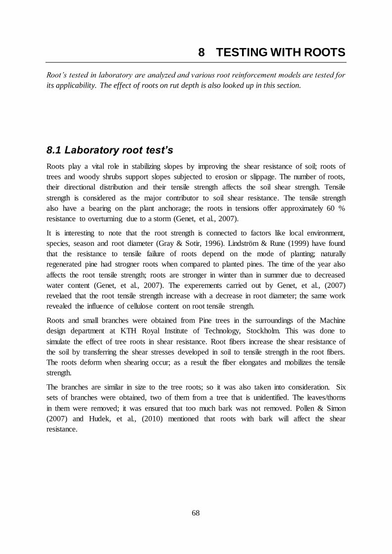
68

8 TESTING WITH ROOTS

Root’s tested in laboratory are analyzed and various root reinforcement models are tested for

its applicability. The effect of roots on rut depth is also looked up in this section.

8.1 Laboratory root test’s

Roots play a vital role in stabilizing slopes by improving the shear resistance of soil; roots of

trees and woody shrubs support slopes subjected to erosion or slippage. The number of roots,

their directional distribution and their tensile strength affects the soil shear strength. Tensile

strength is considered as the major contributor to soil shear resistance. The tensile strength

also have a bearing on the plant anchorage; the roots in tensions offer approximately 60 %

resistance to overturning due to a storm (Genet, et al., 2007).

It is interesting to note that the root strength is connected to factors like local environment,

species, season and root diameter (Gray & Sotir, 1996). Lindström & Rune (1999) have found

that the resistance to tensile failure of roots depend on the mode of planting; naturally

regenerated pine had strogner roots when compared to planted pines. The time of the year also

affects the root tensile strength; roots are stronger in winter than in summer due to decreased

water content (Genet, et al., 2007). The experements carried out by Genet, et al., (2007)

revelaed that the root tensile strength increase with a decrease in root diameter; the same work

revealed the influence of cellulose content on root tensile strength.

Roots and small branches were obtained from Pine trees in the surroundings of the Machine

design department at KTH Royal Institute of Technology, Stockholm. This was done to

simulate the effect of tree roots in shear resistance. Root fibers increase the shear resistance of

the soil by transferring the shear stresses developed in soil to tensile strength in the root fibers.

The roots deform when shearing occur; as a result the fiber elongates and mobilizes the tensile

strength.

The branches are similar in size to the tree roots; so it was also taken into consideration. Six

sets of branches were obtained, two of them from a tree that is unidentified. The leaves/thorns

in them were removed; it was ensured that too much bark was not removed. Pollen & Simon

(2007) and Hudek, et al., (2010) mentioned that roots with bark will affect the shear

resistance.

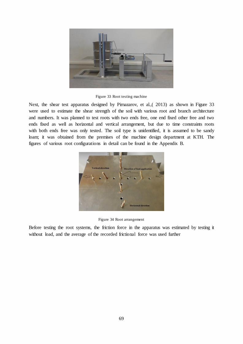
69

Figure 33 Root testing machine

Next, the shear test apparatus designed by Pirnazarov, et al.,( 2013) as shown in Figure 33

were used to estimate the shear strength of the soil with various root and branch architecture

and numbers. It was planned to test roots with two ends free, one end fixed other free and two

ends fixed as well as horizontal and vertical arrangement, but due to time constraints roots

with both ends free was only tested. The soil type is unidentified, it is assumed to be sandy

loam; it was obtained from the premises of the machine design department at KTH. The

figures of various root configurations in detail can be found in the Appendix B.

Figure 34 Root arrangement

Before testing the root systems, the friction force in the apparatus was estimated by testing it

without load, and the average of the recorded frictional force was used further

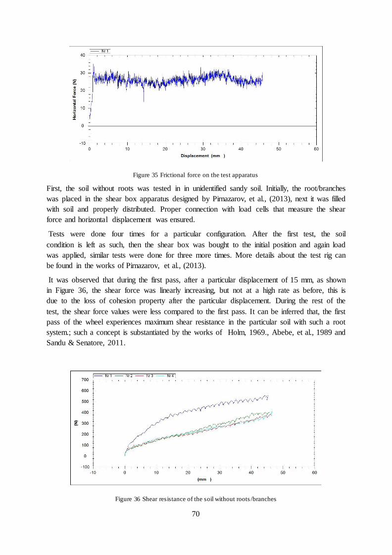
70

Figure 35 Frictional force on the test apparatus

First, the soil without roots was tested in in unidentified sandy soil. Initially, the root/branches

was placed in the shear box apparatus designed by Pirnazarov, et al., (2013), next it was filled

with soil and properly distributed. Proper connection with load cells that measure the shear

force and horizontal displacement was ensured.

Tests were done four times for a particular configuration. After the first test, the soil

condition is left as such, then the shear box was bought to the initial position and again load

was applied, similar tests were done for three more times. More details about the test rig can

be found in the works of Pirnazarov, et al., (2013).

It was observed that during the first pass, after a particular displacement of 15 mm, as shown

in Figure 36, the shear force was linearly increasing, but not at a high rate as before, this is

due to the loss of cohesion property after the particular displacement. During the rest of the

test, the shear force values were less compared to the first pass. It can be inferred that, the first

pass of the wheel experiences maximum shear resistance in the particular soil with such a root

system.; such a concept is substantiated by the works of Holm, 1969., Abebe, et al., 1989 and

Sandu & Senatore, 2011.

Figure 36 Shear resistance of the soil without roots /branches

71

Similar results were obtained for test’s done with one branch with both ends free, here, the

shear resistance was maximum for the first pass and it decreased for the consecutive passes.

Figure 37 Shear resistance of soil with one branch

Next test were done for branches with both ends free, the number of branches used were 2,

arranged horizontally. The shear force during the first go with two branches (or first test) was

similar to the first test result as shown in Figure 37 of test with one branch, theoretically,

when the number of roots increase the shear force must increase according to Equation 27, if

the roots are identical, the shear force must be twice, which is not the case. This shows the

variation between the theoretical and original test data, but it has to be noted that the equation

is exclusively for roots.

Figure 38 Shear resistances of 2 root branches in horizontal position

i i ir

T n at

A

(27)

Where,

rt = mobilized tensile force of roots per unit area

72

iT = ultimate tensile strength of roots

in = number of roots

ia = mean cross sectional area of the roots

A = area of the shear plane

Next four branches were arranged in horizontal orientation, Figure 39 shows the results

obtained; the first pass produced the maximum shear force, further passes produced low shear

force values compared to the first pass.

Figure 39 Shear resistances of 4 branches in horizontal position

The other set of tests include, arranging two roots in vertical direction with both ends free.

The results were similar to normal test, wherein, the first test produced maximum shear force.

During the next test, where four roots were arranged in vertical direction with both ends free,

the shear resistance of first pass was high compared to all other tests mentioned above. The

possible explanation for this behavior is, the movable middle box had contact with the first

root in vertical orientation, this root –tire interaction increased the shear force. When the tire

is not in contact with the roots, that is, when the roots are at a certain depth below the soil tire

interface, the shear resistance offered is not high as when they are in contact with the tire.

Figure 40 Test results with four branches in vertical orientation

A new series of test was done again; the soil cohesion and internal angle of soil friction was

obtained with the available apparatus designed by Pirnazarov, et al., (2013), but the direct

73

shear test method was a crude one and did not follow the ASTM D3080 shear test standard.

Here, fresh soil was obtained from the premises of KTH Machine design department, the soil

type was not identified, but its texture represented the forest soil.

The data’s of the experiments were saved and then it was used to compare with analytical

models. The first test average shear force was compared to the ones calculated theoretically.

All the calculations were done in Matlab

During the second series of test with new soil, one additional test was done for the 1st go of

the machine to obtain more data values. When one root was tested in the new soil type, it

displayed behavior that is completely different from what was seen in the previous tests. Here

after a particular value of shear displacement, the shear force of the consecutive passes

displayed a rise as shown in Figure 41.

Figure 41 Test results with one root tested in new soil type

Similar results were obtained for tests with 2, 4 and 8 number of roots, for both vertical and

horizontal orientation. It was observed that the maximum shear force from the new soil type is

low compared to the sandy soil. Even with eight roots, the new soil shear resistance could not

match the one offered by sandy textured soil. This shows the contribution from soil type and

roots on the shear resistance.

Figure 42 Results with 4 roots in horizontal position in new soil type

74

Figure 43 Results with 4 roots in vertical position in new soil type

Figure 44 Results with 8 roots tested in new soil type

Also, a test was done to get an idea about the compaction the forest soil encounters, during

loading. For this test, an aluminum plate was kept in the apparatus mentioned before and then

filled with soil as usual. After that load was applied to estimate the resistance offered to

compaction. From the test, it was observed that, after a particular displacement, a peak in

resistance was observed as seen in Figure 45, this is assumed to be due to the aluminum plate

interfering with soil particles and as a result offering high resistance; once that obstacle is

overcame, the trend became normal. Otherwise, an almost linear rise in resistance is observed.

Figure 45 Compaction test results with aluminum plate

From Figure 46, it can be seen that when then number of roots are two, vertical arrangement

offer more shear resistance, but when the number of roots are four, horizontal arrangement

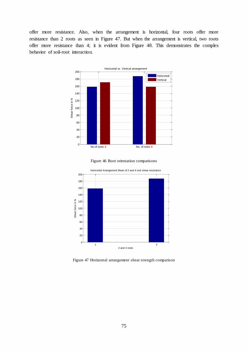
75

offer more resistance. Also, when the arrangement is horizontal, four roots offer more

resistance than 2 roots as seen in Figure 47. But when the arrangement is vertical, two roots

offer more resistance than 4; it is evident from Figure 48. This demonstrates the complex

behavior of soil-root interaction.

Figure 46 Root orientation comparisons

Figure 47 Horizontal arrangement shear strength comparison

No.of roots 2 No. of roots 40

20

40

60

80

100

120

140

160

180

200Horizontal vs. Vertical arrangement

Shear

forc

e in N

Horizontal

Vertical

1 20

20

40

60

80

100

120

140

160

180

200

Horizontal Arrangement Mean of 2 and 4 root shear resistance

2 and 4 roots

Shear

forc

e in N

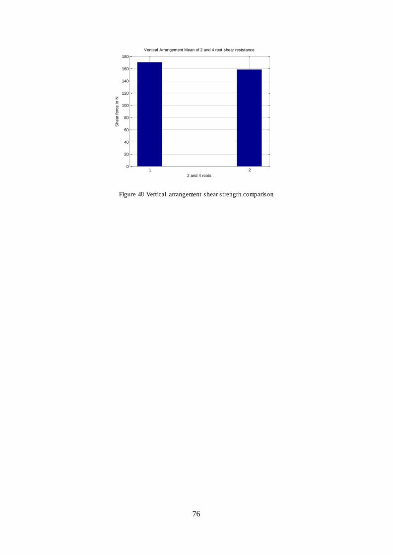
76

Figure 48 Vertical arrangement shear strength comparison

1 20

20

40

60

80

100

120

140

160

180

Vertical Arrangement Mean of 2 and 4 root shear resistance

2 and 4 roots

Shear

forc

e in N

77

8.2 Root reinforcement analysis

The root reinforcement to the soil, as mentioned before, has been analyzed through lab tests.

In this section, theoretical models available are utilized to estimate the reinforcement provided

by roots to the soil. The models used include; perpendicular root model developed and tested

by Wu (1976) and Waldron (1977), the model proposed by Abe & Ziemer, (1991) and the

root stretch model developed by Gray & Barker (2013); these models are widely used to

quantify the root reinforcement.

In the perpendicular root model, the shear stress is magnified by a horizontal element of the

tensile stress (Tn), as shown in the Figure 49. This model assumes that the roots are well

anchored and do not out when a tensile force is applied; this model is more suitable when the

roots are in the ‘fiber break mode’ (Gray & Barker, 2013).

Figure 49 Perpendicular root reinforcement model

The total shear strength of the soil and roots can be calculated with the equation:

tansr rS c S (28)

1.2r rS T RAR (29)

rT D (30)

Where,

Scr = total shear strength of the soil and roots

c=soil cohesion value

= normal stress acting on the soil

=soil internal friction angle

Sr = increased shear resistance provided by the roots

Tr = Root tensile strength

RAR = Root area ratio

78

, = empirical value depending on species

Here two sets of , have been investigated, the first one, 23.40 and -0.87, proposed by

Andre, et al., 2011 and 12.42 and -0.69, proposed by Hudek, et al., 2011.

As mentioned before, another model proposed by Abe & Ziemer, 1991 was also studied to

assess the shear strength prediction capability. According to Abe & Ziemer, 1991, the extra

reinforcement provided by roots come from its tensile stress and shear strength applied to a

root by earth pressure. The model proposed by them is given as:

tansrS c AS (31)

1/2

2 2 2 31 1 cos tan sinbx

rAS B b e Ea EIb B

(32)

Where,

AS= reinforcement provided by roots in Pa

B= one half of shear displacement in m

b= best fitting parameter

x= half length of the root in m

E=Young’s modulus of the root in Pa

ra = cross sectional area of the root in m2

I= section modulus of the root in m3

= tan-1(Bb)

In the experiments carried out, it was noticed that the roots didn’t break after the test. So, it is

more feasible to apply the ‘fiber stretch mode’ analysis to estimate the reinforcement provided

by the roots. The mobilized tensile strength will depend on the amount of fiber elongation and

fiber tensile modulus when the fiber lacks enough elongation and strain compatibility issues

forestall mobilization of root tensile strength (Gray & Barker, 2013). The extra reinforcement

provided by roots to the shear strength of soil is given by Equation 33:

sin cos .tanRAS k

A

(33)

4 b Rz E

kD

(34)

sec 1 (35)

1 sin tanb h f (36)

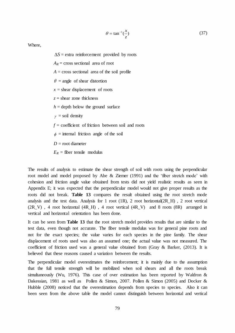
79

1tan ( )x

z (37)

Where,

S = extra reinforcement provided by roots

AR = cross sectional area of root

A = cross sectional area of the soil profile

= angle of shear distortion

x = shear displacement of roots

z = shear zone thickness

h = depth below the ground surface

= soil density

f = coefficient of friction between soil and roots

= internal friction angle of the soil

D = root diameter

ER = fiber tensile modulus

The results of analysis to estimate the shear strength of soil with roots using the perpendicular

root model and model proposed by Abe & Ziemer (1991) and the ‘fiber stretch mode’ with

cohesion and friction angle value obtained from tests did not yield realistic results as seen in

Appendix E; it was expected that the perpendicular model would not give proper results as the

roots did not break. Table 13 compares the result obtained using the root stretch mode

analysis and the test data. Analysis for 1 root (1R), 2 root horizontal(2R_H) , 2 root vertical

(2R_V) , 4 root horizontal (4R_H) , 4 root vertical (4R_V) and 8 roots (8R) arranged in

vertical and horizontal orientation has been done.

It can be seen from Table 13 that the root stretch model provides results that are similar to the

test data, even though not accurate. The fiber tensile modulus was for general pine roots and

not for the exact species; the value varies for each species in the pine family. The shear

displacement of roots used was also an assumed one; the actual value was not measured. The

coefficient of friction used was a general value obtained from (Gray & Barker, (2013). It is

believed that these reasons caused a variation between the results.

The perpendicular model overestimates the reinforcement; it is mainly due to the assumption

that the full tensile strength will be mobilized when soil shears and all the roots break

simultaneously (Wu, 1976). This case of over estimation has been reported by Waldron &

Dakessian, 1981 as well as Pollen & Simon, 2007. Pollen & Simon (2005) and Docker &

Hubble (2008) noticed that the overestimation depends from species to species. Also it can

been seen from the above table the model cannot distinguish between horizontal and vertical

80

orientation, as it gives the same value for both the cases of 2 roots and 4 roots in horizontal

and vertical arrangement.

New cohesion and friction angle values were obtained by doing tests in the available machine

as mentioned before, friction angle was estimated to be 48.79 degrees and cohesion was 1134

Pa. With the new cohesion and internal friction angle calculations were done, but it yielded

results similar to the one obtained using the one retrieved from Wong’s (Wong, 2010)

literature. It has to be noted that the method employed to obtain the cohesion and internal

friction angle did not follow the shear testing standard; but it was adopted to get an idea about

where the values would lie.

Table 13 Shear strength of soil with roots in kPa: Test data vs. root reinforcement models

Arrangement 1R 2R_H 4R_H 2R_V 4R_V 8R

Test 0.8 1.9 2.8 2.12 2.72 1.10

Root-stretch 1.891 1.892 1.901 1.892 1.907 1.905

Abe & Ziemer 8.9 1.3 21.8 11.3 21.8 NA

In the perpendicualr model, the value of cohesion and friction angle significantly influences

the results.So when the model is used in situations where the roots break, it should be ensured

that the cohesiona dn friction angle values used should be obtained from laboratory tests.

Abe and Ziemer equation was used, but ‘b’, value obtained through equation proposed Abe &

Ziemer, (1991) didn’t yield realistic results, so the values obtained from the tests by Abe &

Ziemer, (1991) was used. The same value has been used for all the root diameters, even

though the value changes according to the empirical equation proposed in the literature.

From the analysis it was found that, the test data results and analytical results didn’t match

well. The value of cohesion and internal friction angle of the soil was not known accurately. It

was noticed that the when the value of cohesion and friction angle was changed, it affected

the test results significantly. Also it can been seen from the above table the model cannot

distinguish between horizontal and vertical orientation, as it gives the same value for both the

cases of 2 roots and 4 roots in horizontal and vertical arrangement.

But it is evident that the Root stretch mode provides results that are more realistic and

comparabe with the test data as compared to the Abe and Ziemer model. It can therefore be

conluded that the root stretch model provides good estimate when the root does not break. As

a suggestion, it is prescribed to do more test with roots and obtain a coeffcient describing the

diffrence between the two orientations and apply it to a thoeretical model that could predict

the results well.

81

8.3 Rut depth comparison with and without roots

The rut depth produced by one vehicle pass of Rottne loaded with 450 kPa estimated from

various WES models has been compared with the rut depth estimated by the same WES

models when root reinforcement also comes into effect. The constants used in all the WES

models are obtained from non-linear regression analysis as mentioned in section 4.3.1.

In this method, new cone index when roots are present has been obtained, and this value has

been applied in the WES models to estimate the rut depth with roots. As expected all the

models returned low value of rut depth when roots are taken into account. The WES models

used includes the ones proposed by, Maclaurin, Antilla, Saarilahti and Rantala.

The root present was assumed to be of Casuarina glauca and the corresponding extra

reinforcement provided by roots has been estimated from:

61.16 0.90S RAR (38)

Where,

S = extra reinforcement by roots

RAR = root area ratio

The resistive force acting on a penetrating cone can be obtained from Equation 39 (Baladi & Rohani, 1981) and Figure 50.

0

( tan )2 tan

L

ZF d (39)

2

4 ZFCI

D

(40)

Where,

Fz =cone resistive force

= normal stress

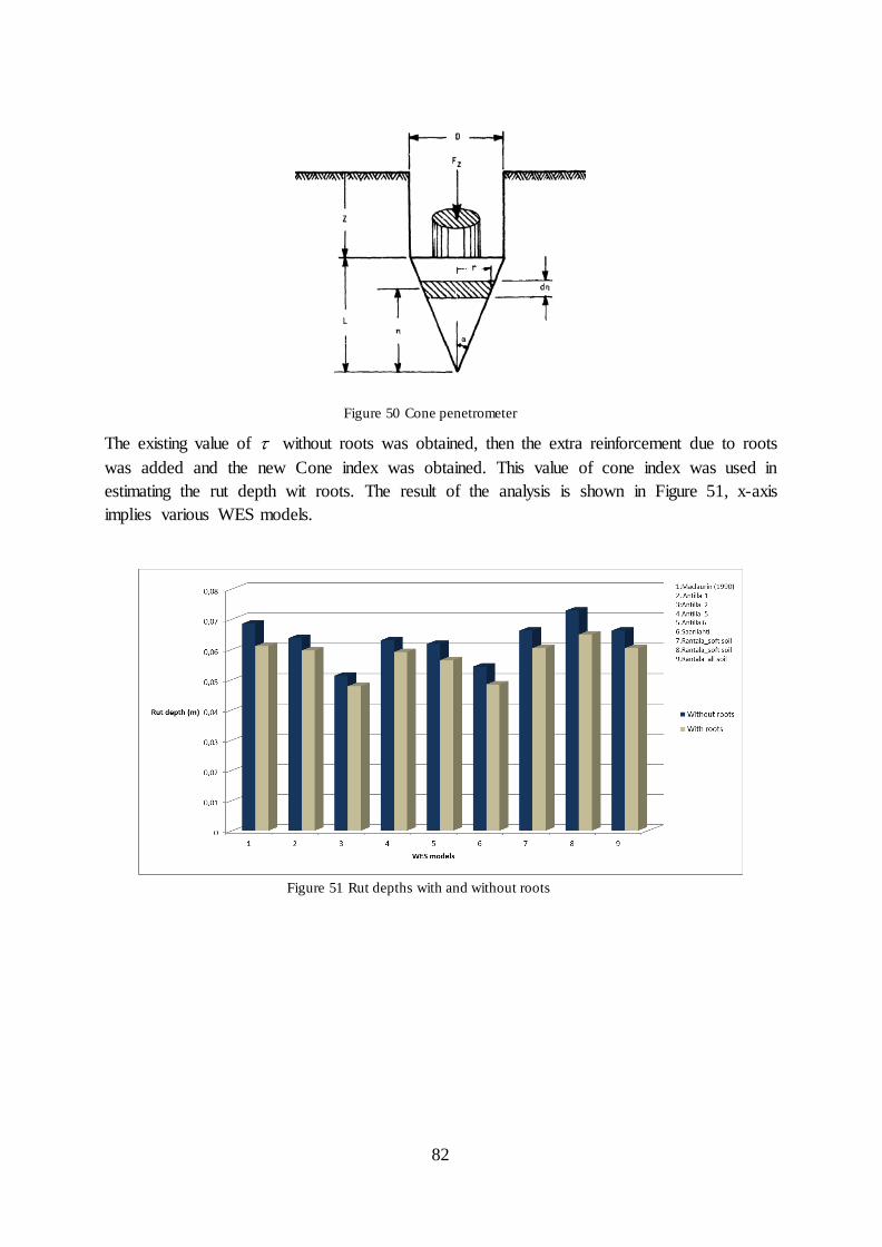
82

Figure 50 Cone penetrometer

The existing value of without roots was obtained, then the extra reinforcement due to roots

was added and the new Cone index was obtained. This value of cone index was used in

estimating the rut depth wit roots. The result of the analysis is shown in Figure 51, x-axis

implies various WES models.

Figure 51 Rut depths with and without roots

83

8.4 Analysis of test data from lab root test

The test data from the lab test of the soil, newly collected, with roots have been analyzed. In

the light of non-compatibility of available root reinforcement models, curve fitting approach

with least squares method has been adopted to derive empirical equations for the

corresponding tests. The results of the test data has been presented in Figure 52. A linear

equation has been derived.

y a bx (41)

Where,

y= shear resistance in N

x= displacement

a and b = empirical constants

Table 14 Coefficients of the empirical relation

Configuration a b R2 (%)

1 root 84.6 25.5 92

2 root horizontal 279.6 4.34 95

4 root horizontal 17.98 8.5 99

2 root vertical 343.8 4.34 86

4 root vertical 406 5.83 90

8 roots 127.2 2.761 75

Figure 52 Diagram depicting the displacement vs. shear resistance of 2- root horizontal arrangement

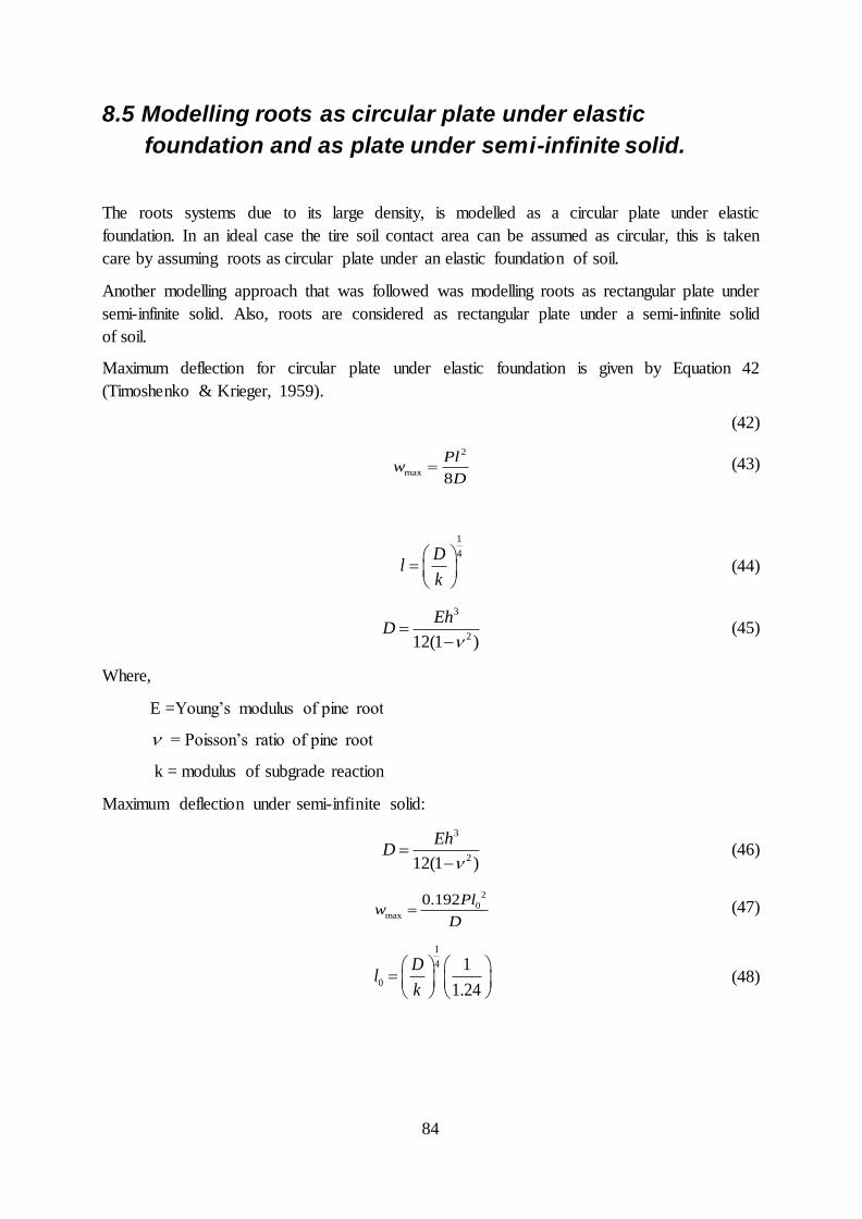
84

8.5 Modelling roots as circular plate under elastic

foundation and as plate under semi-infinite solid.

The roots systems due to its large density, is modelled as a circular plate under elastic

foundation. In an ideal case the tire soil contact area can be assumed as circular, this is taken

care by assuming roots as circular plate under an elastic foundation of soil.

Another modelling approach that was followed was modelling roots as rectangular plate under

semi-infinite solid. Also, roots are considered as rectangular plate under a semi-infinite solid

of soil.

Maximum deflection for circular plate under elastic foundation is given by Equation 42

(Timoshenko & Krieger, 1959).

(42)

2

max8

Plw

D (43)

1

4Dl

k

(44)

3

212(1 )

EhD

(45)

Where,

E =Young’s modulus of pine root

= Poisson’s ratio of pine root

k = modulus of subgrade reaction

Maximum deflection under semi-infinite solid:

3

212(1 )

EhD

(46)

2

0max

0.192Plw

D (47)

1

4

0

1

1.24

Dl

k

(48)

85

The rut depth due to various loads when roots are present in the above configuration is shown

in Figure 53. The maximum deflection of the center part of the plates is considered as the

maximum rut depth that could be produced when a wheel passes over such a material.

Figure 53 Load vs. Rut depth

It can be seen from the figure that, there is not much difference in the rut depth predicted by

the two root configuration. More studies into the root configurations needs to be carried out to

find a good model to simulate the effects of root or how roots can be modelled; FEM can be

employed to delve more into studying the effects when roots are modelled as circular plate

under elastic foundation and as plate under semi-infinite solid. Phenomenon’s like cracking

and sliding of roots can be studied with the help of DEM.

16 18 20 22 24 26 28 300.03

0.035

0.04

0.045

0.05

0.055

0.06

0.065

Load (kN)

Rut

depth

(m

)Roots modelled as Circular plate and plate resting on semi-infinite solid

Circular plate

Plate on semi infinite soild

86

9 Slip Sinkage Effect

The effect of slip on the sinkage is dealt in this chapter. Sinkage at various slip levels has been

studied here.

The increase in sinkage and motion resistance due to slip if referred as slip-sinkage effect.

The influence slip-sinkage effect on vehicle sinkage and motion resistance is gaining

momentum; before, much publication did not take into account this effect (Lyasko, 2009).

Slip sinkage effect on wheel sinkage due to a single wheel has been studied here; the work of

Lyasko (Lyasko, 2009) is the main inspiration. The necessity of predicting the accurate value

of sinkage has been highlighted in the work of Lyasko (Lyasko, 2009). Works of Lyasko

shows that for slip range from 0 to 33 % the sinkage increase monotonically and for 33% slip

the increase is about 60%.

Lyasko, found the analytical Equation 49, between the sinkage and the slip of the wheel.

0SSz K z (49)

1

1 0.5SS

iK

i

(50)

Where,

z = sinkage due to slip

z0 = static sinkage

i = slip

In the original work, Lyasko (2009), the static sinkage of the wheel has been obtained using

the Nernstein-Goriatchkin equation with the help of test data, the detailed method can be

found in Lyasko, 2009.

Here, in the thesis, the slip and sinkage affecting one wheel on the first axle is taken into

account. Because, as mentioned by Abebe, et al., 1989 and Sandu & Senatore 2011, passes

one to three of a single wheel produces the maximum sinkage or rut depth.

WES based approach and Bekker based approach has been tried on the slip sinkage effect. On

analysis of both the models with respect to slip sinkage, it has been found that the sinkage

increases as slip increases. But both models gave almost the same results for sinkage values as

seen in Figure 54. Such an approach can be used to estimate the intesity of sinkage due to

slippage and fine tune the slip values. It will be good to do a real field test to evaluate which

model gives results that are same as tets results, to be more precise with the models.

87

Figure 54 Slip-Sinkage effect

The static sinkage has been obtained using WES and Bekker based equation as described

below.

0 1.25

0.224

CI

z dN

(51)

Bekker model:

1/

0 1/

( )/

( )/ b

n

wt

c t

n

wt

c

pif l b

k l kz

pif l b

k k

(52)

1

4 1

1.24t

Dl

k

(53)

Where,

pw = wheel pressure

tl = length of wheel flat section

b = wheel width

t = wheel deflection

0 0.05 0.1 0.15 0.2 0.25 0.3 0.35 0.40.012

0.014

0.016

0.018

0.02

0.022

0.024

Slip

Sin

kage in m

Slip-Sinkage effect: WES vs. Bekker Model

WES

BEKKER MODEL

88

9.1 Estimating rut depth based on single wheel test

Another approach that has been tried is to utilize the result from a single wheel test and utilize

it for multi-pass rut depth prediction; the analysis was carried out for Komatsu and the results

were compared to test data.

Here, the maximum load acting on any wheel of the vehicle is taken into account, and then

this load is applied into Maclaurin (1990) WES model by taking into account the slip acting

on that wheel. The importance of slip-sinkage is explained in the above section, and it

simulates the real tire-soil interaction situation.

The wheel with maximum load acting will produce the highest sinkage in static condition, and

this sinkage can be taken as a yardstick to evaluate various vehicles. Here, the result of such

an analysis for the entire vehicle configuration, as described in Table 2, has been done. The

results of which are shown in Figure 55, except for S-shaped curves, the results are fairly

matching to the test data.

To evaluate the model’s validity further, the same analysis has been applied to S curves also,

but with the difference that the rut depth values at the straight portion was only taken into

account and compared to WES models as seen in Figure 56. It can therefore be seen from the

results that the new approach could predict the rut depth with reasonably good accuracy.

Figure 55 Calculated rut depths vs. Test data (conditions 4, 5 11 and 12 are S-shaped tracks)

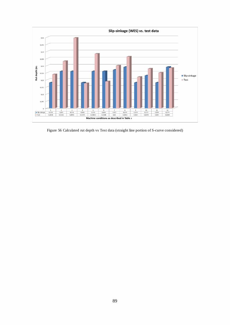
89

Figure 56 Calculated rut depth vs Test data (straight line portion of S-curve considered)

90

10 Co-relating WES and Bevameter models

A small step towards co-relating WES and Bekker based models has been carried out here. A

new set of equations has been derived and available relations are also evaluated in this

section.

Both the WES and Bevameter models, as explained before, have different input variables. For

Nordic forests, it has been proposed by Saarilahti, that WES models could provide suitable

results. The multibody simulation software MSC Adams uses Bekker based Bevameter

approach to solve tire - soft soil interaction analysis. Also, many studies have been done with

the aid of Bevameter data’s. But the number of variables in the Bekker based model is many,

when compared to WES models.

In this section, a study to co-relate both WES and Bekker based model is carried out. Two

models have been derived to connect Cone index and Bekker constants. The models proposed

below is applicable for a single wheel for one pass, as the 1st pass produce the maximum

impact to the ground or rut depth.

The first model, it is applicable to sandy silt soils, the parameter ‘n’, dimensionless exponent

of load-sinkage curve, is taken as one. At the end of the analysis, it has been verified that the

estimated Bekker’s cohesive and friction moduli of soil deformation of load-sinkage curve,

kcand kφ, from the cone index value gives back the same value on ‘n’. The explanation is

given below:

According to Kalugin and Poletaev (Lyasko, 2010), the sinkage of the first wheel is:

2

3

1

3

2

Wz

Bk D

(54)

Rearranging Equation 54

1.6

1

3

(2 )z

Wk

B D (55)

Equation 56 gives the WES based sinkage model which can be applied to Equation 55, this

will result in connecting k with cone index.

1

0.6100.010

CI

zN

(56)

91

According to Garbari (Lyasko, 2010), the motion resistance of the first wheel is given by:

2

1

2

kBzMR (57)

Motion resistance can also be written as:

RMR W (58)

The motion resistance coefficient can be expressed in terms of Cone index as proposed by

Ashmore et al (1987), also the sinkage can be calculated using the relation proposed by

Rantala (2001) as given by Equation 56. Equation 59 express motion resistance in terms of

wheel numeric NCC.

0.21

0.380 0.50 0.21R

r CC

W

W N

(59)

CC

CIbdN

W h

(60)

Equating Equation 57 and Equation 58, and on rearranging gives Equation (61);

2

1

2 RWkBz

(61)

Where, R is a function of cone index as seen from Equation (59) :

Also,

ckk k

B (62)

ck k k B (63)

And finally, applying Equation 55 and Equation 61 into Equation 63 results in connecting kc

with cone index. In a nutshell, the relations can be described as shown below:

1n (64)

1.6

1

3

2

Wk

B Dz (65)

92

21.6

11

23

2

Rc

WWk B

BzB Dz

(66)

In the second model, an empirical model connecting kc and kφ, has been obtained. Then the

equation connecting Cone index and kφ obtained from the previous model has been used. By

combining both the models, the value of kc, has been obtained. This model is applicable to all

soils, but, it has to be noted that this model is an empirical model and can be applied to soil

conditions at Tierp, where the data’s were obtained, but not extrapolated to other conditions.

The empirical relation connecting kc and kφ, is:

5 27.6 10 0.032 122.6ck k k

(67)

From the Equation 55, we know;

1.6

1

3

(2 )z

Wk

B D (68)

The value of ‘n’ is estimated using the equation:

2

2 13

(3 )( )

n

c

Wz

n k Bk D

(69)

It has to be noted the equations so derived, from both the models, have not been verified. It is

highly suggested to tests with soils to determine the capability of the equation. A specified

amount of load has to be applied in single wheel tester and simulate a single wheel pass.

Specified sample of soil has to be collected, and its cone index has to me measured. The same

sample of soil has to undergo a Bevameter test to determine the Bekker constants. After that

all the values obtained should be used to evaluate the equations.

Another approach done to co-relate both WES and Bekker models were to compare the ratio

of rut depths given by WES and Bekker models. Two approaches were invested as part this

procedure.

In the first approach, the equation connecting Cone index to Bekker parameters, as proposed

by Bekker (Bekker, 1969), was used to estimate the Cone index value for various Bekker

parameter values. The Bekker parameter values for Upland sandy loam soil was used, the

values were fetched from Wong’s literature (Wong, 2010). Then sinkage value for a single

wheel was estimated using Bekker’s equation. With the calculated Cone index values, sinkage

for the wheel was calculated with WES based models. Here, the soil parameter only changes,

not the load acting on the wheel. The results of the analysis are shown in Figure 58. The

relation connecting Cone index to Bekker model is given by the Equation 70..

93

2 2 1

1 11.5 ( 1.5)

1.625 1.5 0.517( 1) ( 1)( 2) 2 1

n n nn nc

zk z z zCI z z k

n n n n n

(70)

Various values of moduli of soil deformation and sinkage exponent for Upland sandy loam

has been used as shown in the Figure 57.

Figure 57 Bekker parameters for various soils

The WES model used for evaluating is the one proposed by McLaurin, Rantala and Gee-

Glough. The results of which are shown in Figure 58, the x axis shows the various soil

conditions described by Bekker parameters. It can be seen that only the Gee-Glough model

provides a ratio that is almost near to one, but as it does not experience a trend in the graph, it

is hard to find a constant that connects both the models.

The WES equations used are:

Maclaurin:

1.25

0.224

CI

z dN

(71)

Rantala’s (2001) equations for soft soils and all soils:

1.25

0.224

CI

z dN

(72)

94

0.490

0.059CI

zN

(73)

1.23

0.989

CI

zN

(74)

Gee-Glough’s:

2

0.63 0.34

0.287

R

R

CI

dz

b

b

N

(75)

Where

z= sinkage in m

R = rolling resistance coefficient

Figure 58 Correlating WES and Bekker model at different soil conditions

In the second approach, the ratio of sinkage calculated from WES and Bekker models for

various load conditions were calculated. Here, the values of Bekker parameters used were

obtained from the Bevameter tests carried at Tierp, the Cone index values were also obtained

from test done at Tierp.

The results of the above mentioned analysis is shown in Figure 59, the x axis shows the

various load conditions. Here also, it was hard to find a model that was equal or almost near

to one.

1 2 3 4 5 6 7 8 9 10 11-0.2

-0.15

-0.1

-0.05

0

0.05

0.1

0.15

Points

Diffe

rence in S

inkage (

m )

Maclaurin-Bekker

Rantala 1 - Bekker

Rantala 2 - Bekker

Gee-Glough-Bekker

1 2 3 4 5 6 7 8 9 10 110

0.5

1

1.5

2

2.5

3

3.5

4

Points

WE

S /

Bekker

Sinkage WES = Constant x Sinkage Bekker

Maclaurin / Bekker

Rantala 1 / Bekker

Rantala 2 / Bekker

Gee-Glough / Bekker

95

Figure 59 Correlating WES and Bekker model at different load conditions

0 5 10 15 20 25 300

0.2

0.4

0.6

0.8

1

1.2

1.4

Load (kN)

Sin

kage W

ES

/ S

inkage B

ekker

Sinkage WES = Constant x Sinkage Bekker

Maclaurin / Bekker

Gee-Glough / Bekker

Rantala / Bekker

Saarilahti / Bekker

Saarilahti 2 / Bekker

Saarilahti 3 / Bekker

96

11 ADAMS Multi-body Simulation

MSC Adams software has been used to simulate a full-scale forwarder models to see its

effectiveness in predicting rut depths. Single wheel tests have also been carried out to

estimate the effect of tire inflation pressure and velocity on rut depths.

As part of the master thesis work, MSC Adams is used to simulate the effect of multi-pass of

the forwarder. Adams has a module called Soft-Soil tire model; this module can be used to

simulate the interaction between tires and elastic/plastic grounds like sand, clay, snow and

loam .This model uses a tire property file and a road data file with soil properties. Adams

offer two types of tire soil contact models:

Elastic-plastic soil deformation model

Visco-Elastic soil deformation model

In the thesis work, elastic-plastic deformation mode has been used throughout the simulations.

11.1Adams Tire

Adams tire is a separate module that helps simulate tire-soil interaction. It computes the forces

action on a tire moving over a roadway or irregular terrain. Dynamic response of vehicles

performing activities like acceleration, steering braking etc. can be obtained (MSC Software,

2014).

Adams/Tire can be used with Adams/Car, Adams/Chassis, Adams/Solver or Adams/View. In

this thesis work, Adams/Tire is employed in Adams/View. Adams/Tire consists of a set of

shared libraries which Adams/Solver calls through subroutines. These subroutines, namely,

DIFSUB, GFOSUB, GSESUB, compute the moments and force that the tire exert on the

vehicle due to tire-terrain interaction. Adams/Tire has a set of tire modules that could be used

to model rubber tires. The five modules present in Adams/Tire are (University of Bergamo,

2014).

Adams/Tire Handling Module

Adams/Tire 3D Spline Road Module

Adams/Tire 3D Shell Road Module

Specific Tire Models

Features in Adams/Tire modules.

97

The basic steps involved in Adams/Tire are shown in Figure 60.

Figure 60 Basic steps followed by Adams/Tire

The three processes that occur when a tire is added to Adams model are (University of

Bergamo, 2014):

Adams/Solver activates Adams/Tire

Adams/Tire determines the tire and road model to use

Adams/Tire does the calculations for the tire model

The above mentioned process is graphically represented in Figure 61.

Figure 61 Processes that occur after tire is added to the model

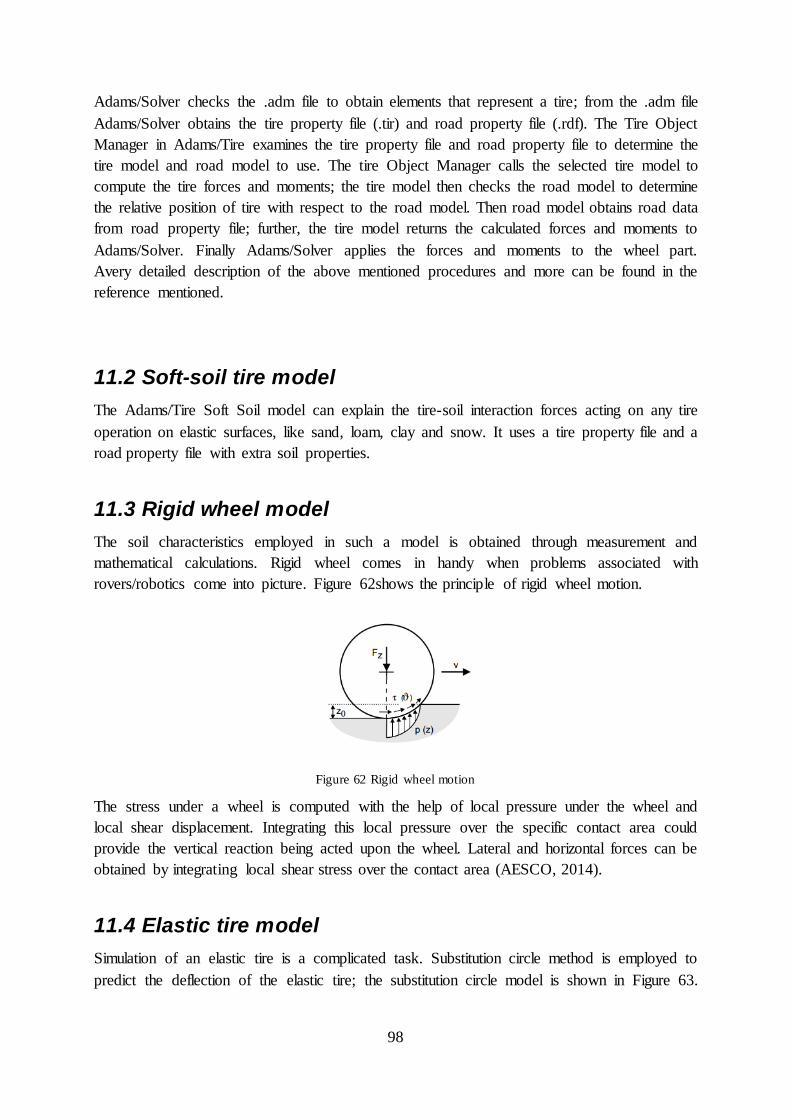
98

Adams/Solver checks the .adm file to obtain elements that represent a tire; from the .adm file

Adams/Solver obtains the tire property file (.tir) and road property file (.rdf). The Tire Object

Manager in Adams/Tire examines the tire property file and road property file to determine the

tire model and road model to use. The tire Object Manager calls the selected tire model to

compute the tire forces and moments; the tire model then checks the road model to determine

the relative position of tire with respect to the road model. Then road model obtains road data

from road property file; further, the tire model returns the calculated forces and moments to

Adams/Solver. Finally Adams/Solver applies the forces and moments to the wheel part.

Avery detailed description of the above mentioned procedures and more can be found in the

reference mentioned.

11.2 Soft-soil tire model

The Adams/Tire Soft Soil model can explain the tire-soil interaction forces acting on any tire

operation on elastic surfaces, like sand, loam, clay and snow. It uses a tire property file and a

road property file with extra soil properties.

11.3 Rigid wheel model

The soil characteristics employed in such a model is obtained through measurement and

mathematical calculations. Rigid wheel comes in handy when problems associated with

rovers/robotics come into picture. Figure 62shows the principle of rigid wheel motion.

Figure 62 Rigid wheel motion

The stress under a wheel is computed with the help of local pressure under the wheel and

local shear displacement. Integrating this local pressure over the specific contact area could

provide the vertical reaction being acted upon the wheel. Lateral and horizontal forces can be

obtained by integrating local shear stress over the contact area (AESCO, 2014).

11.4 Elastic tire model

Simulation of an elastic tire is a complicated task. Substitution circle method is employed to

predict the deflection of the elastic tire; the substitution circle model is shown in Figure 63.

99

Equilibrium between the vertical reaction force from the soil and vertical reaction from tire is

used to obtain the diameter of the substitute circle, D* (AESCO, 2014).

Figure 63 Substitution circle method

11.5 Elastic/plastic deformation of the soil

The deformation experienced by the soil as result of loading by tires consists of an elastic part

and a plastic part (MSC Software, 2013).Soil elasticity values used are very important in such

simulations, especially for multi-pass computations. As a result more exact and realistic

values associated with pressure distribution under wheels can be obtained. Elastic behavior of

soil in this module is adapted from Wong’s work (Wong, 2010), here the stiffness is assumed

to be linear over the entire range of sinkage (AESCO, 2014).

11.6 Visco-elastic tire soil contact

This is another mode of taking into account the tire-soil interaction in Adams soft-soil tire

model. Here, for multi-pass effect, the deformation of the road at the exit of tire-soil contact is

stored. The rut depth after a tire pass is obtained by correcting with relaxation effect the road

deformation (MSC Software, 2013).

11.7 Observations in Adams soft soil

For the one wheel model as well as the full scale model of Komatsu 860, it was noticed that,

when the models are in equilibrium position the tire/tires sink to a specific depth into the soil.

It was observed that, this sinkage depend upon the amount of load applied to the respective

wheel; as the load increases the sinkage increases as can be seen from the.

This position gives the static equilibrium position of the system and returns the static sinkage

of the tires. When the simulation was carried out, for both single tire and the Komatsu model,

it was observed that the output sinkage was the same as obtained in equilibrium.

This observation is something that is different from what is observed in reality, what can be

interpreted from Adams results is that the sinkage value remains the same as observed during

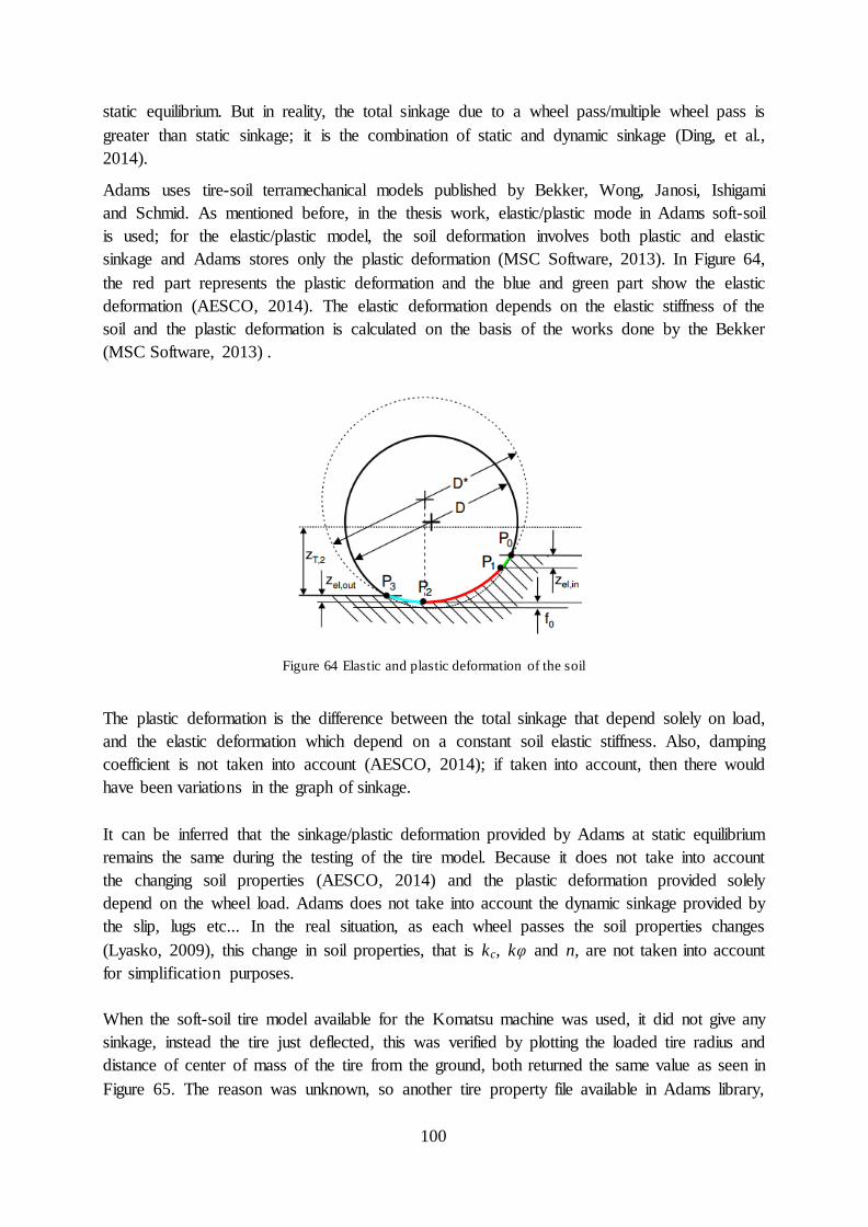
100

static equilibrium. But in reality, the total sinkage due to a wheel pass/multiple wheel pass is

greater than static sinkage; it is the combination of static and dynamic sinkage (Ding, et al.,

2014).

Adams uses tire-soil terramechanical models published by Bekker, Wong, Janosi, Ishigami

and Schmid. As mentioned before, in the thesis work, elastic/plastic mode in Adams soft-soil

is used; for the elastic/plastic model, the soil deformation involves both plastic and elastic

sinkage and Adams stores only the plastic deformation (MSC Software, 2013). In Figure 64,

the red part represents the plastic deformation and the blue and green part show the elastic

deformation (AESCO, 2014). The elastic deformation depends on the elastic stiffness of the

soil and the plastic deformation is calculated on the basis of the works done by the Bekker

(MSC Software, 2013) .

Figure 64 Elastic and plastic deformation of the soil

The plastic deformation is the difference between the total sinkage that depend solely on load,

and the elastic deformation which depend on a constant soil elastic stiffness. Also, damping

coefficient is not taken into account (AESCO, 2014); if taken into account, then there would

have been variations in the graph of sinkage.

It can be inferred that the sinkage/plastic deformation provided by Adams at static equilibrium

remains the same during the testing of the tire model. Because it does not take into account

the changing soil properties (AESCO, 2014) and the plastic deformation provided solely

depend on the wheel load. Adams does not take into account the dynamic sinkage provided by

the slip, lugs etc... In the real situation, as each wheel passes the soil properties changes

(Lyasko, 2009), this change in soil properties, that is kc, kφ and n, are not taken into account

for simplification purposes.

When the soft-soil tire model available for the Komatsu machine was used, it did not give any

sinkage, instead the tire just deflected, this was verified by plotting the loaded tire radius and

distance of center of mass of the tire from the ground, both returned the same value as seen in

Figure 65. The reason was unknown, so another tire property file available in Adams library,

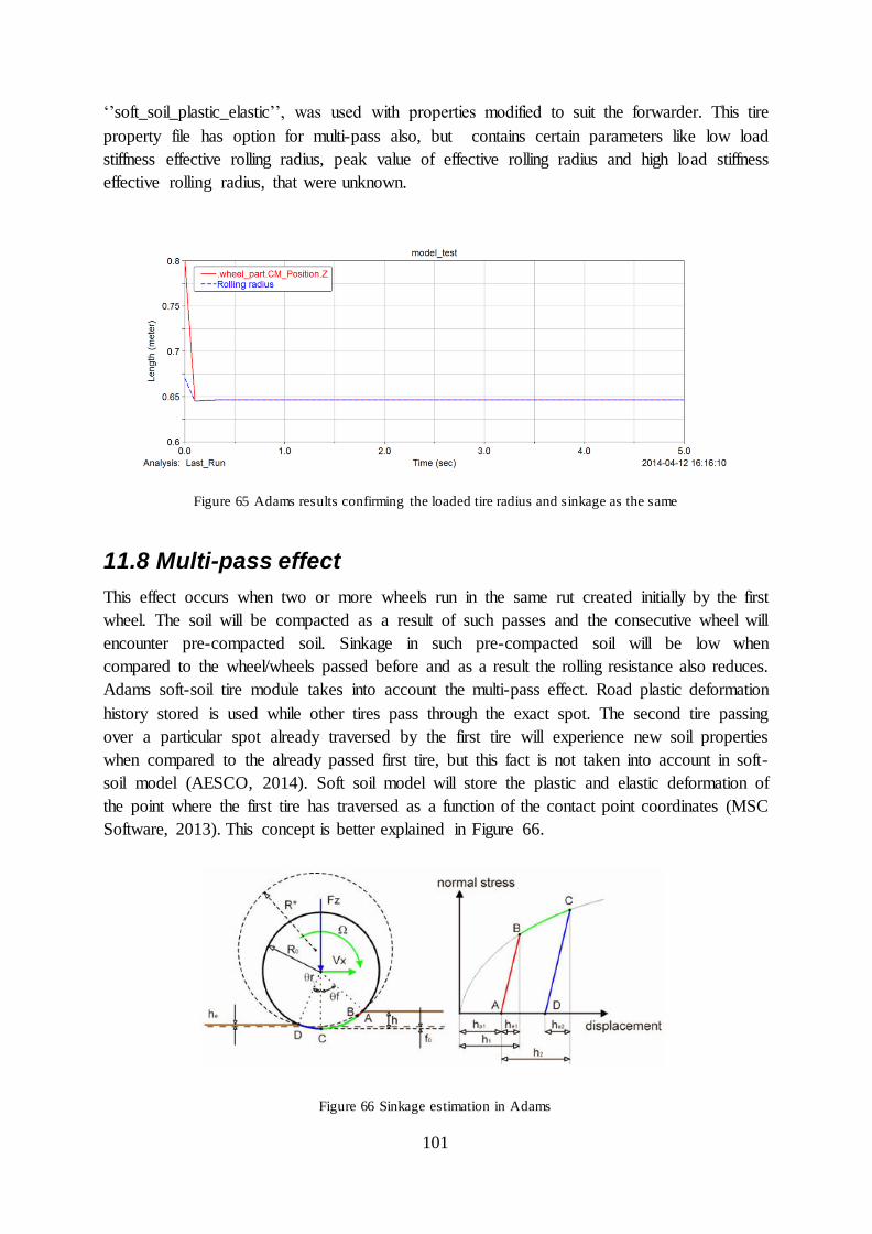
101

‘’soft_soil_plastic_elastic’’, was used with properties modified to suit the forwarder. This tire

property file has option for multi-pass also, but contains certain parameters like low load

stiffness effective rolling radius, peak value of effective rolling radius and high load stiffness

effective rolling radius, that were unknown.

Figure 65 Adams results confirming the loaded tire radius and sinkage as the same

11.8 Multi-pass effect

This effect occurs when two or more wheels run in the same rut created initially by the first

wheel. The soil will be compacted as a result of such passes and the consecutive wheel will

encounter pre-compacted soil. Sinkage in such pre-compacted soil will be low when

compared to the wheel/wheels passed before and as a result the rolling resistance also reduces.

Adams soft-soil tire module takes into account the multi-pass effect. Road plastic deformation

history stored is used while other tires pass through the exact spot. The second tire passing

over a particular spot already traversed by the first tire will experience new soil properties

when compared to the already passed first tire, but this fact is not taken into account in soft-

soil model (AESCO, 2014). Soft soil model will store the plastic and elastic deformation of

the point where the first tire has traversed as a function of the contact point coordinates (MSC

Software, 2013). This concept is better explained in Figure 66.

Figure 66 Sinkage estimation in Adams

102

Take into account two tires, one rolling after the other through the same spot. The first tire

will produce an elastic deformation he1 and a plastic deformation hp1, adding to a total

deformation of h1.

The second tire passing over the same spot will produce an elastic deformation from A to B

(=he1). The plastic deformation of second tire hp2 is equal to the total deformation h2

subtracted from the elastic deformation he2.

The plastic deformation is calculated as:

Plastic deformation= eh h

( )me

s

hC

(76)

*

0 0( , , )h f R R f (77)

Where,

eh = elastic deformation

h = total sinkage

0f = tire deflection

The coordinates, as well as elastic and plastic deformation and tire width of each tire will be

stored. Single point of contact approach is used in soft-soil tire model; the stored values of

deformation will be used as a new tire comes into contact with the rut generated by the

previous tire pass. So, when a tire encounters the point passed by another tire, the tire just

encounters the same virgin terrain at a depth produced by the first terrain, without taking into

account the changed soil properties. It has been assumed in the calculations that soil strength

parameters will not be changed, in reality it does and can be seen in the work done by M.

Lyasko 2009 and Sandu and Senatore 2011, this assumption has been made to simplify the

computations and reduce the soil parameters (AESCO, 2014).

11.9 Connecting Adams results with WES models

An attempt was carried out to connect the results from Adams simulation with the WES

models. A simple approach was experimented, loaded single wheel at various loads ranging

from 10 kN to 24 kN was tested in Adams, the results of which was compared with the WES

models.

The soil property values, namely, the cohesive modulus of sinkage (kφ), friction modulus of

sinkage (kc) and the exponent of sinkage (n) obtained from the bevameter tests at Tierp,

Sweden was used in the Adams soft soil road property file. Other values in the soil property

file were left as such, because they were not known. The corresponding, value of Cone index

103

was used in WES calculations. The WES models used were the ones proposed by Maclaurin,

Antilla, Gee-Glough and Rantala.

Figure 67 Soft-soil/Tire model in Adams

Results obtained from Adams were exported to Matlab and analyzed. The ratio of sinkage

results at various loads from WES models and Adams results were taken to obtain a constant

that connects both the results. From Figure 68 , it can be seen that the Antilla model connects

well to the Adams results; the ratio is almost near to one. An average of the ratio between

Antilla and Adams model, that is, 0.83, can be used to connect both the models. Here the soil

condition is assumed to be same, while the load varies.

In the above analysis, the slip-sinkage effect has not been taken into account; it has already

been discussed in Section 9 about the importance of slip-sinkage effect. Taking the slip into

account in the WES model provides a more realistic result; for that, another comparison the

same Adams results and WES model with slip-sinkage incorporated has been done and the

results can be seen in Figure 68, here the constant 1.10 connects WES and Adams results.

It has to be noted that, bevameter tests for various soils has to be obtained, to determine the

soil stiffness constants as well as exponent of sinkage and inputted to the soft soil road

property file along with soil friction angles, soil cohesion stress, soil stiffness and soil

deformation modulus to determine the reliability of the constants proposed. Sinkage for each

load case starting from 10 kN till 24 kN, as measured from Adams results is shown in Figure

69.

104

Figure 68 Comparison between Adams result and WES results with/without slip -sinkage

Figure 69 Single wheel test results for various loads from Adams

10 12 14 16 18 20 22 240

0.5

1

1.5

2

2.5

3

3.5

4

4.5

Load in kN

WE

S M

odel /

Adam

s m

odel

Sinkage WES = constant x Sinkage Adams

Maclaurin/Adams

Gee-Glough/Adams

Rantala Soft soil 1/Adams

Rantala Softsoil 2/Adams

Rantala-All soils/Adams

Antilla/Adams

10 12 14 16 18 20 22 240.5

1

1.5

2

2.5

3

3.5

4

4.5

5

5.5

Load in kN

WE

S M

odel /

Adam

s m

odel

Sinkage WES (slip-sinkage) = constant x Sinkage Adams

Maclaurin/Adams

Gee-Glough/Adams

Rantala Soft soil 1/Adams

Rantala Softsoil 2/Adams

Rantala-All soils/Adams

Antilla/Adams

105

11.10 Simulation of the Komatsu 860.3 model

The Komatsu 860.3 CAD model was imported to Adams View 2012, then a simulation was

run to determine the rut depth created by the vehicle pass.

Figure 70 Komatsu 860.3 model imported to Adams View 2012

The model, as seen in Figure 70, was available for unloaded version of the forwarder; proper

pressure value of 600 kPa was inputted to the tire property file. The machine was simulated;

but the simulation was not as smooth and had issues with equilibrium. The model exhibited

unstable behavior during major portion of the simulation time and then provided a stable

sinkage value. The results of the simulation in Adams for the right side tires are shown below

in Figure 71.

Figure 71 Comparison of Adams, WES and Test data for Komatsu unloaded 600 kPa

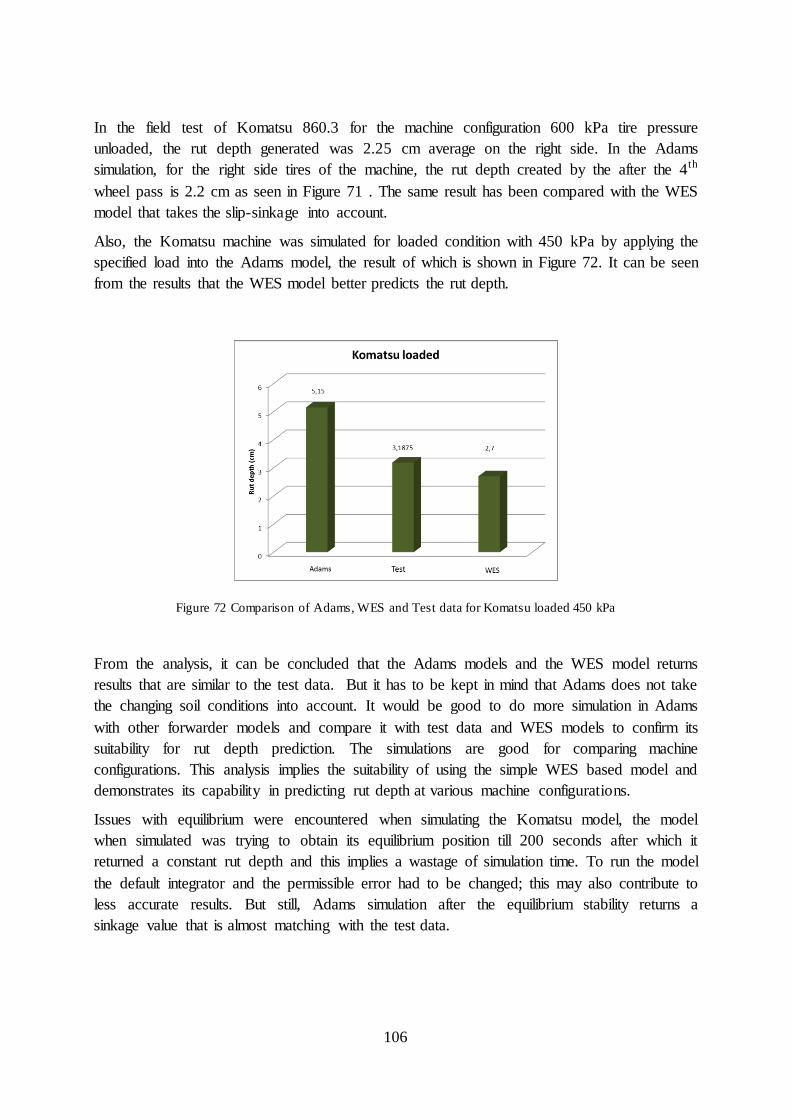
106

In the field test of Komatsu 860.3 for the machine configuration 600 kPa tire pressure

unloaded, the rut depth generated was 2.25 cm average on the right side. In the Adams

simulation, for the right side tires of the machine, the rut depth created by the after the 4th

wheel pass is 2.2 cm as seen in Figure 71 . The same result has been compared with the WES

model that takes the slip-sinkage into account.

Also, the Komatsu machine was simulated for loaded condition with 450 kPa by applying the

specified load into the Adams model, the result of which is shown in Figure 72. It can be seen

from the results that the WES model better predicts the rut depth.

Figure 72 Comparison of Adams, WES and Test data for Komatsu loaded 450 kPa

From the analysis, it can be concluded that the Adams models and the WES model returns

results that are similar to the test data. But it has to be kept in mind that Adams does not take

the changing soil conditions into account. It would be good to do more simulation in Adams

with other forwarder models and compare it with test data and WES models to confirm its

suitability for rut depth prediction. The simulations are good for comparing machine

configurations. This analysis implies the suitability of using the simple WES based model and

demonstrates its capability in predicting rut depth at various machine configurations.

Issues with equilibrium were encountered when simulating the Komatsu model, the model

when simulated was trying to obtain its equilibrium position till 200 seconds after which it

returned a constant rut depth and this implies a wastage of simulation time. To run the model

the default integrator and the permissible error had to be changed; this may also contribute to

less accurate results. But still, Adams simulation after the equilibrium stability returns a

sinkage value that is almost matching with the test data.

107

11.11 Effect of tire inflation pressure on sinkage

The tire inflation pressure can affect both the topsoil and upper subsoil stress distribution

(Keller & Arvindsson, 2004). The tires are designed in such a way that they should be used at

a specific inflation pressure and a specific load. It has been shown by Arvindsson & Ristic,

1996, that the rut depth will increase with the tire inflation pressure. It is evident from

Bekker’s work as well from other tests (Szymaniak & Pytka, u.d.) that, as the inflation

pressure decreases the rut depth also decreases. At low inflation pressure, the tire deflects

more due to increased contact area, as a result contact pressure reduces. Pronounced effect of

inflation pressure is seen at lower velocities (Szymaniak & Pytka, u.d.).

The effect of tire inflation pressure on sinkage has been studied by simulating a single wheel

tester. The wheels were simulated on conditions depicting Upland sandy loam and Rubicon

sandy loam. Sinkage values were obtained for a constant load of 21.82 kN and for tire

pressures, 270 kPa, 450 kPa and 600 kPa. Also, the sinkage values were compared to the

sinkage obtained when the manufacturer prescribed tire pressure was used for the particular

load. The results are shown in Figure 73 and Figure 74.

Figure 73 Sinkage for various tire inflation pressures in Upland sandy loam

Figure 74 Sinkage for various tire inflation pressures in Rubicon sandy loam

108

From the results it can be inferred that, the sinkage increases as the tire inflation pressure

increases. And, it is advisable to use the manufacturer specified tire inflation pressure to

reduce the sinkage. The sinkage at pressures 200 kPa, 220 kPa, 300 kPa, 400 kPa, 450 kPa

and 600 kPa was studied for Upland sandy loam as seen in Figure 75.

Figure 75 Sinkage for various tire inflation pressure in Upland sandy loam

After the simulation, the results were analyzed in Matlab and a linear relationship was found

between the tire inflation pressure and sinkage, the relation can be described as:

81 0.00359y x (78)

Where

y= sinkage in mm

x= tire inflation pressure in kPa

Figure 76 Linear relationship between tire inflation pressure and tire sinkage

109

11.12 Effect of velocity on rut depth

The velocity of the wheel affects factors like wheel sinkage, wheel slip, net tractive ratio,

gross tractive ratio, tractive efficiency etc. From the works of many authors, it can be asserted

that velocity should be taken into account while studying tire-soil interaction. To control the

performance of off-road vehicles, a general model that is capable of taking into account the

changing velocity is needed (Shmulevich, et al., 1998).

Grahn, 1991 concluded from his works on sandy loam that the rut depth decreases as the

velocity increases. There are also other studies that indicate reduction in rut depths when the

vehicle velocity increases (Szymaniak & Pytka, u.d.). Whereas, Liu, et al., 2009, from their

field test on a Heavy Expanded Mobility Tactical Truck concluded that the rut depth increases

as the velocity of the vehicle increases. The tests conducted by Crenshaw, 1972 showed that

at high speed (higher than 93 km/h) and low speeds (0-37 km/h), as the velocity is increased

the rut depth decreases; but at intermediate-speeds (0-37 km/h), as the velocity is increased

the rut depth also increases.

So, to get an idea about how the wheel velocity affects the rut depth, a simulation was carried

out in Adams. Single wheel with an inflation pressure of 160 kPa was tested in Upland sandy

loam with a load of 21.82 kN at various velocities. The results of which are shown in Figure

77.From the results, it can be inferred that, Adams does not taken into account the effect of

velocity. For all the velocities, it gives the same sinkage, unlike reality. As a result, the

velocity effect on sinkage was not properly studied with Adams as it only takes into account

the static sinkage This can be considered as flaw that needs to be rectified, if the software has

to been used in prediciting accurate rut depths.

Figure 77 Wheel velocity vs. wheel sinkage simulated in Adams

110

12 DISCUSSION AND CONCLUSIONS

Various aspects of work done as part of the thesis and the conclusion derived from the study

are discussed here.

12.1 Rut depth

From the analysis of the rut depths with the available models for single wheel pass, it can be

concluded that, the single pass rut depth models are not suitable for estimating the rut depths

caused by a forwarder.

To counter the above mentioned issue, new coefficient’s has been obtained through regression

analysis for the existing single wheel pass rut depth models to take care of the multi-pass

effect of the forwarder’s, Rottne 13S and Komatsu 860.3. It is suggested to use the existing

WES based models with the new coefficient obtained through regression analysis.

Maclaurin’s, Antilla’s model 1,2,3 and Rantala’s model can be used to give a better prediction

as those model gives the least mean square error. But it has to be noted that the new

coefficients are applicable only for the specific terrain and machine conditions; it should not

be extrapolated to other terrain and vehicle conditions.

With the application of the Novel wheel mobility number, the rut depth prediction was

enhanced, especially for the Komatsu 860.3. With more test data, the capability of the model

could be estimated. This model also has the drawback of being an empirical model and as a

result cannot be extrapolated. But, from the results obtained, it can be inferred as a good

model.

The variation of constants in WES based models has been studied. It was noted that the

constants depend on the soil characteristics, the constants varied when the cone index/cone-

index range was varied. The constants displayed the same value for a range of cone index

values.

The Abebe model that takes into account the multi-pass effect of wheels has been studied.

The original model developed by Abebe was for the multi-pass of same wheels with same

load. As a result, that model cannot be applied in the case of the forwarders, due to the

varying load on each wheel. So, non-linear regression analysis has been carried out to obtain

new values of multi-pass coefficient’s that could take care of the situation of varying wheel

loads. The use of regression analysis to estimate the best fit parameters implies the use of the

model only in the specific conditions. The Abebe model with the new coefficients can predict

rut depth better than the single wheel pass models.

During multi-pass of wheels, each following wheel will experience a new soil condition

different from the wheel passed before it. This issue has been taken into account by

computing the new cone index after each wheel pass, and this new cone index values has been

111

used to estimate the rut depth after each wheel pass and the cumulative rut depth due to the

vehicle pass has been estimated. From the analysis, it was noted that the model give results

that are good be taken into account, even though not accurate. This is due to the inherent

assumptions applicable to the model that computes the varying cone index. But, this model

takes into account the realistic situation of changing soil parameters that are not available in

other models.

The Kharkhuta’s model was employed to estimate the rut depth due to multi-pass effect of

wheels primarily because of the simplicity of the model. But, it was found that the model

gives poor results. The Kharkhuta’s coefficient should be determined after tests in soil, but

here, the coefficient used has been the average of values obtained from literature. This is

considered as the primary reason for unsatisfactory results.

An empirical equation to connect the change in rut depth percentage with changing cone

index has been obtained. This empirical relation can be used in the future for estimating the

change in rut depth percentage with change in cone index percentage. It is suggested to

evaluate the efficiency of the relation by doing more multi-pass tests and cross-checking the

test data with the calculated results.

Finally, an empirical relation connecting the cone index with depth of measurement has been

obtained. From the analysis, the range of values that the coefficients can take has been found

out. This equation has the potential to act a good empirical model for finding the cone index

at Tierp provided the depth of measurement till 21 cm. Liner equations were proposed even

though the trend exhibited was not exactly linear; the reason is to make the equations simpler

and reduce the coefficients.

All the empirical models discussed, with the new coefficients can be used to determine the rut

depth’s with reasonable accuracy and these models can be used as yardstick to select various

machine configurations. None of the models can act as a general equation to determine the rut

depth; this is mentioned to show that the empirical models cannot act as general model in any

parameter analysis. As a suggestion, to estimate the effectiveness of all the approaches and

analysis carried out, more field tests with varying loads, machine conditions and soil

conditions has to be carried out.

According to Jun, et al., 2004, the soil compaction is dependent on the tire-soil contact

pressure. Edlund, et al., 2012, has shown that the forwarder steering and transmission drive

system also affects the rut depths. Liu, et al., 2009 has demonstrated the effects of vehicle

weight, type, velocity, turning radius, soil texture and soil moisture content affetcs the depth

of ruts. A comprehensive model that takes all these factors into account, as well as varying

soil conditions, would be more realistic and may provide accurate result. Incorporating the

shearing effect due to trailer tires in forwarder has to be addressed by looking into the relation

between the trailer turning radius and the wheel torque.

112

12.2 Pressure

The surface pressure felt by the soil due to wheel load has been studied. Various models

proposed by Saarilahti, 2002, has been analysed. It was observed that the Schwanghart (1990)

model was in line with the pressure predicted by dividing the wheel load with measured area

for Rottne. In case of Komatsu, , MMP Moist clay 1, MMP Moist clay 2, Disern’s (2008) 1,

Disern’s 2008 (2) and Duttmann (2012) provided similar results. Whereas, the model Per

(2010) provided similar result to the pressure measured at 15 cm below ground level for

Rottne. Ground pressure index, Empirical, Keller (2005) and Disern’s (2011) 2 models

provided similar result to the measured pressure value at 15 cm for Komatsu. It has been

understood that no model could predict the exact value at the tire soil interface and there was

no measured value also to compare with. Reviewing various literatures showed that, still there

exist confusions in measuring accurate surface pressure values.

It would be good to obtain the pressure at tire-soil interface, and make a comparison with the

available models. Values obtained from pressure cells that are placed at low depth give more

insight into the contact pressure values. The pressure sensor can be configured in a way

similar to placing the load cells as suggested by Lamande, et al., 2007, the sensor can be

placed in a specially made cylinder so that it has more contact area and better measurements

can be made. Figure 78 shows the construction of the cylinder.

Figure 78 Cylinder designed by Lamande, et al., 2007

The cylinder is made up of two parts, when one part is pushed it displaces relative to the other

part and results in a wider diameter. Such an action could cause a good contact between the

soil and the load cell.

Also, the load cell arrangement as used by Lamande´ & Schjønning, 2011, can be used to get

a better estimate of the contact pressure at the tire-soil interface. This would provide more

realistic values to compare the pressure obtained through various models. Also, the suitability

of the models for predicting pressure in the specific terrain can be assesed.

113

Figure 79 Surface sensor arrangement by Lamande et al., 2007

One of the best methods that can be employed to get an almost accurate value of surface is the

one used by Cirello, et al., (2009) were chromatic impression technology is employed. The

chromatic filim, know as Prescale film ( brand name), is attached between the tire and ground.

When the load is applied, the film varies among various shadings of magenta, the internsity of

which is directly proportional to the applied load/pressure: the darker color corresponds to

higher pressure and vive-versa. The value of pressure can be obtained with the help of a

special software. A series of tests at various load levels and at a constant pressure can be done

and an empirical relation can be derived, to aid in the surface pressure prediction in Noridic

soil conditions.

Figure 80 Tire footprint on a Prescale paper

Figure 81 Color density of magenta

The pressure distribution is always not uniform under a tire, the work done by Jun, et al.,

2004, demonstrates that when the correct combination of dynamic load and inflation pressure

exist, the pressure distribution is relatively uniform. The same work emphasises the use of

correct inflation pressure for the specific load to reduce tire-soil contact pressure as well as

soil compaction.

114

The surface pressure also depends on the tire load and tire inflation pressure. But as the tire

load increases, the recommended tire inflation pressure increases. This creates a situation

where both the parameters cannot be studied independently.

If the pressure value at a certain depth can be considered as standard value to compare the soil

damage induced due to heavy machines, measurement’s would be easy as compared to

surface pressure measurement.

The cone index value at a particular depth along a line has to be measured, along the same

line at the same depth, the pressure can also be measured by load cells. Such an analysis at

various types of soils has to be carried out. It would be good to connect the cone index and

measured pressured to gain an insight about the dependence of cone index and pressure.

12.3 Contact area

Various models have been analyzed to predict the tire-soil contact area of the forwarders. The

results have been compared with the measured area, by multiplying the measured length and

breadth of the contact patch. It has to be noted that, the measured contact area does not

provide the accurate contact patch area, but a rough value only suitable for comparison.

Finally, the super-ellipse model was also studied the results were compared with the measured

value.

Few models provided values that are close to the measured values. But they cannot

completely be regarded as good predictor, as the measured area is only a rough estimate and

not an accurate value. By using image processing techniques the real contact area can be

calculated, it would be good to compare various models with this original area and determine

the best models.

Work done by various researchers suggests the use of the super-ellipse model as good

indicator of accurate contact patch area. The study with super ellipse in the thesis also point to

that direction. It can therefore be concluded that, super-ellipse model is good predictor of tire-

soil contact area.

To exactly determine the contact area, advanced technologies like image processing can be

used. The technology is promising and good results have been obtained by applying such

technology to obtain the tire soil contact area in a single wheel tester at Urmia University

(Mardani & Taghavifar, 2013). Also techniques involving capturing the images of contact

area and further analyzing it in an image processing software and finally using a planimeter to

obtain the area is also being used and provides a good estimate of the contact area, this

method has been explored by Mardani & Taghavifar, 2012.

12.4 Mobility parameters

From the results obtained for the wheel numerics of the both Rottne and Komatsu; for Rottne,

the models Turnage (1972a), WESLAB, Wismer and Luth (1973), Maclaurin (1990),

Maclaurin (1990_rounded wheel numeric gives similar result for drawbar pull coefficient. For

115

Komatsu, the models, N.I.A.E Model, Brixiuis (1987), Maclaurin (1990) and Maclaurin

(1990_rounded wheel numeric) gives similar results for drawbar pull coefficient.

The rolling resistance provided by most of the models except, N.I.A.E Models and Ashmore

et al (1987) for Rottne gives similar results. For Komatsu also, both N.I.A.E Models and

Ashmore et al (1987) provide results that are dissimilar to other models.

When cone index range from 200 kPa to 1160 kPa are taken into account, it can been seen

that the models Wismer and Luth, Rummer and Ashmore, Maclaurin, Maclaurin new,

McAllister and Bruce Maclaurin gives similar results.

As the models, Maclaurin (1990) and Maclaurin (1990_rounded wheel numeric/new), provide

reliable results for both drawbar pull coefficient and rolling resistance coefficient, these two

models can be used to find out the mobility parameters of the machines at all times. As a word

of caution, it has to be noted that the models are empirical.

It would be good to do field tests in real machines in the specified cone index range and

compare the results with the theoretical model, so that certain models can be always be used

to predict the mobility parameters.

12.5 Roots

Laboratory tests have been carried out to study the reinforcement effect provided by roots to

the soil. Two types of soils were used along with branches and roots of pine trees to evaluate

their strengthening effects. The results showed variation in the characteristics of the shear

force measured; the sandy textured soil with pine branches exhibited higher shear resistance

when compared to the other soil with pine roots. It was concluded from the tests that the

combination of soil and roots affect the shear strength of the roots. The shear resistance

offered by the soil also depends on the root number and configuration; it was evident from the

analysis that when the number of root were 2, the vertical arrangement offered more shear

resistance; while the horizontal arrangement offered more shear resistance when the number

of roots were 4.

The measured shear force obtained from the machined designed by Pirnazarov, et al., (2013)

was compared to the results obtained from the perpendicular model, Abe & Ziemer, (1991)

model and finally the root strech model. The perpendicular models over estimated the values

when compared to the measured data.The perpendiucular model used by both Andre, et al.,

(2011) and Hudek, et al., (2010) had already received comments from various authors about

its overestimation trend, plus the model is only suitable when the root breaks

The model developed by Abe & Ziemer, (1991) has been based on one shear plane, but test

rig used for the experiment has two shear planes. The values of cohesion and internal angle of

friction for the soils were obtained from laboratory tests in the equipment designed by

Pirnazarov, et al., (2013). Also a constant in the model has been obtained from literature. It is

assuemd that these may be the reasons that contributed to the oversetimation by the model.

The root stretch model provided good results. This model simulated the exact conditions in

the test carried out; because the roots didn’t break and it only stretched. The results, even

116

though comparable, was not accurate. The possbile resasons include, usage of general fiber

tensile modulus for pine roots, assumed shear displacement and the coefficient of friction.

The soil cohesion and friction angle has to be determined through lab tests that follow the

standard ASTM D3080 to obatin the accurate value. Similar tests have to be carried out to

find the Youngs modulus, coeffcient of friction between roots and soil and finally the shear

displacement of roots; this will help to bring the results more close to test data.

It was noticed that the equations used to predict the reinforcement due to roots cannot

differentiate between the orientation of the roots that is whether they are horizontal or vertical.

This is a major flaw in the equations. One remedy can be to obtain an average value of ratio

between the horizontal and vertical arrangement, then apply this ratio to a best fit equation

that describes the reinforcement effects due to roots.

When using the perpendicular model, the root average root tensile strength has to be measured

by tensile tests and it has to be utilized to obtain the correct value of average tensile strength

of roots per unit area (T. Hubble & Docker, 2008). It has also to be taken into account that

while calculating the reinforcement effect due to roots, the root diameter has to be divided

into classes and analyzed, as is done by Zhou, et al., (1998), Hudek, et al., (2010) etc.

It can be concluded that the perpendicular reinforcement model and Abe & Ziermer model

with the available value of cohesion and internal friction angle of soil cannot be used to

calculate the reinforcement provided by roots to soil when the soil-root combination is tested

in the machine available. But, the root stretch model is promising and can determine the extra

reinforcement provided by the roots.

As a solution to the above mentioned issue of incompatibility perperndicular root model and

Abe & Ziemer model; a set of empirical equations has been developed for the second set of

soil similar to forest soil and pine roots. These equations can be used to predict the shear

resistance offered by the specific soil with pine roots when tested in the machien designed by

Pirnazarov, et al., (2013).

It is highly recommended that more design features has to be incorporated into the machine

designed by Pirnazarov, et al., (2013) such as an actuator to apply a fixed force, proper fixing

mechanism, sheat test apparatus etc. so that it could also act as machine that could be used to

estimate cohesion and internal friction angle values, and this could make the machine more

flexible so that all experiments can be done in a single machine. Data acquisition system can

be programmed to directly output the cohesion and friction angle values.

WES based models was used for the calculation of rut depths with and without roots. The root

of Casuarina glauca was taken into account for the analysis. The results implies a reduction

in rut depth with roots when for the forwarder travel. This shows the importance of root

systems in reducing the rut depths. Rut depth reduction also depend on root architecture and

root distribution .

Roots were modelled as circular plate under elastic foundation and plate under semi-infinite

solid. The results suggest the same rut depth for various load combinations in both cases. The

117

feasibility of the model can only be determined by evaluating the results after a single wheel

test on a pine root matrix at various loads.

Thomas & Bankhead, (2009), suggest the use of fiber-bundle models (FBM) to estimate the

root reinforcment values exactly. According to the works of Thomas & Bankhead (2009), the

constant ‘1.2’ used in the Equation 29 is too large and the value can only be attained if friction

angle is greater than 350. Pollen & Simon (2005) and Pollen, (2007) developed the fiber

bundle model where they take into account the more realistic progressive root failure. The

total load applied to the fiber is allotted to a bundle of N parallel fibers in FBM; then the

fibers are monitored whether the load applied to the nth fivber exceed its strength. Once a

fiber has been broken, then the total load is again redistributed among the remaining fibers.

This approach has provided more accurate estimate of root reinforcement by taking into

consideration the progressive root failure. And even in cases where all the roots break

simultaneously, Pollen & Simon, (2005) found that the perpendicular root model

overestimates the root reinforcement .

In the light of the given root tests, result analysis and from the various works, it can be

concluded that more importance has to be given to FBM models to predict the extra root

reinforcement. FBM analysis on roots growing in the nordic soils would give a new

dimension to reinforcement modelling, as most of the works have been done in North-

American soil.

12.6 Slip-Sinkage

The slip-sinkage effect was studied for a single wheel at various slip to evaluate the effect of

slip on sinkage. Both WES and Bekker based models have been used in the calculations. It

can be concluded that the sinkage will rise as the slip increases.

Another approach to determine the rut depth of the forwarder, Komatsu 860.3, by using slip-

sinkage concept was tried. The slip-sinkage concept proposed by Lyasko, (2009) was used

with the wheel carrying the highest load in the forwarder. The results obtained were quite

satisfactory, even though not accurate, except for S-shaped curves. The suitabilty of the

approach can only be evalauted after comparing results from various tests only. This approach

takes into account the slip also, while other WES based model’s do not. But, within the frame

work of avilable data, the model seems to be promising without involving the complexities

associated with estimatimg multi-pass coeffcient’s.

12.7 WES-Bekker correlation

One of the main challenges in terramechanics is to connect WES model with the Bekker

model. A small step towards solving this problem was taken and a completely new set of

equations has been derived for connecting, the cone index individually with sinkage exponent,

and friction modulus of deformation and cohesive modulus of deformation. One of the

equations can be applied only to sandy textured soils and the other to forest soils. The

118

equations derived have not been verified by lab tests. It is highly recommended to do field

tests in order to see the suitability of the equations.

Bekker has already derived a relation expressing cone index as a function of sinkage

exponent, friction modulus of deformation and cohesive modulus of deformation. This

relation has been assessed for various soil conditions as well as loads and the results showed

that only Gee-Glough WES model complied well with the relation, but not exactly. But more

tests in various soil conditions needs to be done to get a complete picture of which models

could correlate well.

12.8 Multi-body simulation

A detailed investigation into the feasibility of using multi-body simulation software MSC

Adams was done. The various aspects of the soft-soil/tire model were studied and its various

drawbacks were determined. The results from Adams were connected to certain WES models

using a constant.

The software MSC Adams was used to analyze a single wheel in soft-soil condition and also

the full scale Komatsu 860.3 model was simulated to obtain the rut depths created by the

vehicle pass. Only one vehicle pass simulation was carried out on the Komatsu machine, also

the effect of inflation pressure and vehicle velocity on rut depths were studied with the help of

the software.

The results of a single wheel test at various loads were studied and the results were connected

to the WES model proposed by Antilla through a ratio. Analysis was carried by taking into

account sinkage with and without slip. After carrying out a real world test with single wheel

tester, the same approach can be carried out to connect Adams results with test data; as well

as with WES models, this would provide more realistic results by taking care of any error

presented by Adams results. Such an approach would help to create more realistic results

without creating any sub-routine to take care of various changing conditions of soil, but it

involves the job of setting up a single wheel test and applies only to a specific soil type. The

approaches, single wheel test and writing a subroutine has to be evaluated on the basis of

time, complexity and reliability and follow the one that is less demanding on the resources.

Few issues with Adams soft-soil/tire module have been identified. The main issue is that, the

package does not take into account the changing soil parameters due to multipass of wheels;

this is in stark contrast to what happens in reality. During multipass, it provides rut depths that

are actually the static sinkage of the wheels.

During the simulation of the Komatsu model, it was found that the soft-soil module had

issues with equilibrium, it displayed unrealistic behavior for the first 200 seconds as

highlighted in Figure 82, this necessitate the need to delve more into the root cause behind the

issue.

119

Figure 82 Adams simulation result showing the equilibrium issue

Simulation with both unloaded and loaded condition has been carried out and the results were

comparable to the test data and WES model results. This indicates that the both Adams and

WES models could be used for rut depth estimation, but the WES models are simple and does

not involve the intricacies of Adams.

The tire property file in Adams contains certain parameters like low load stiffness effective

rolling radius, peak value of effective rolling radius and high load stiffness effective rolling

radius, that were unknown. Such complications can be avoided by taking into consideration

the WES models, where the only input parameter is the Cone Index. This reinforces the usage

of WES model based subroutines in Adams to tackle the issues associated with tire-soil

interaction. The WES models do not need any parameters that are usually fed to the Adams

soft soil property files also. The Bekker based approach provides a more detailed overview

about calculating various variables like normal stress, longitudinal shear stress, lateral shear

stress, bulldozing effect, grouser effect etc. A subroutine that could incorporate both the

models, even though time consuming, would be appropriate in taking care of multi-pass

effect as well as determining the forces acting on the vehicle traversing on soft soil. But if rut

depth estimation and mobility parameters are given high importance, then a WES based

subroutine is good enough.

Digital elevation model (DEM) techniques can also be taken into account to tackle the issue

of changing soil parameters due to multi-pass effect. With DEM, the soil surface can be

portrayed as a digital elevation grid DEM. Through subroutines the soil parameters of each

grid can be changed as each wheel passes through a set of grids, so that the following wheel

experiences a set of grids with modified soil parameters and simulates non-homogeneous soil

condition. Similar kind of analysis with DEM has been done by Trease, et al (2011) as well as

in the research carried out at the Institute of Robotics and Mechatronics in the German

Aerospace Center (Krenn & Hirzinger, 2009).

The process of changing the grid parameters has been implemented by Pan, et al.(2004) in

their work focussing on creating a complete simulation environment by taking into account all

the models and mobility analysis of vehicles operating in soft-terrain. The same has been

120

implemented by Madesn, et al. (2013) when they developed a model that could take care of

three dimensional deformable terrain in mobility simulation software. Madsen, et al., (2012)

in their work dealing with simulating a terrain vehicle interaction model for a vehicle

simulator has taken care of changing soil parameters by modifying the density of the soil; the

soil density modification has been done by taking into account the time the tire has been in

contact with the soil. In the aforementioned work, the tire soil interaction has been modelled

by physics based analysis where visco-elastic-plastic regimes are taken into account. It would

be good to implement the varying cone index approach for the same mehod mentioned above

and compare the results with test data.

Generating DEM of nordic forest terrain using methods like interferometric synthetic aperture

radar and digital image correlation method and connecting it to Adams to generate terrain

would provide more reliable high fidelity simulations, as it depicts the exact terrain rather

than a user-created terrain.

Adams has been used to study the effect of varying inflation pressure on rut depths at a

constant load with the help of a single wheel. From the analysis, it can be concluded that at a

certain load, the manufacturer recommended tire inflation pressure returns the lowest rut

depth.

An attempt to study the effect of velocity on rut depth was initiated, but the outputs were

same for all the velocities tried. This implies that the software does not take into account the

velocity effects of the wheel.

Fixing the inherent problems with the software are integrating it with more realistic terrain

models, tire models and a subroutine that could take care of varying soil parameters would

assist in improving the performance of high fidelity simulations, which in-turn could generate

more realistic model based designs.

http://en.wikipedia.org/wiki/Interferometric_synthetic_aperture_radar

http://en.wikipedia.org/wiki/Interferometric_synthetic_aperture_radar

121

13 RECOMMENDATIONS AND FUTURE WORK

Recommendations and areas of future work intended to take elevate the tire-soil interaction

analysis to a more detailed level is discussed in this chapter.

Effect of factors like turning radius, velocity and moisture content on rut depth should be

studied. They should be independently studied in various soil conditions to get a broad idea.

The effect of turning radius of trailers and the torque acting on the wheel should be carried out

in various soil conditions as well a machine conditions to get a grip of the various factors

affecting the rut depth in the S-shaped portion. A generalized equation based on such studies

can be developed; implementation of the developed relation into the available WES model

could aid in predicting rut depth accurately in the S-shaped curves.

Soil properties like cohesion and internal friction angle should be obtained through proper

laboratory tests, it is not recommended to use values available from literatures, as soil

properties vary from place to place.

Similarly, the Bekker parameter’s (cohesive modulus of deformation, friction modulus of

deformation and sinkage exponent) used should be obtained through proper bevameter tests.

Using already existing values for similar soil types is not recommended. This helps in giving

proper inputs to Adams road file, which can have a bearing on the predictions.

Contact pressure acting in the tire-soil interface can be studied in detailed by carrying out

field tests. With such tests, the relation of contact pressure on tire inflation pressure, tire

contact area, soil conditions etc.. can be studied in relation to the Nordic conditions. It is

highly recommended to follow the approach intoduced by Cirello, et al., (2009).

Finite element analysis can be carried out to study in detail about the shear stress

reinforcement occurring when the roots are tested in the machine designed by Pirnazarov, et

al., (2013). This will help to derive suitable analytical equations to predict the extra

reinforcement provided by the roots in the soil; this can aid in making the machine a

standardized instrument to test various roots in diffrent soils.

Taking into account the complex calculations of Bevameter approach going into the software;

it is highly recommended to implement a WES based sub-routine that could take care of

various terramechanic parameters in Adams. It also has the advantage of using only the cone

index as the input variable, instead of using the Bekker parameter’s as well as other soil

property values. Implementing the changing soil conditions through a proper subroutine,

either the changing Bekker parameters or the changing Cone index values, in Adams is highly

advocated, this will take the simulation to a more realistic level. If such a subroutine

procedure is developed, it has to be ensured that proper contacts with the MSC experts have to

be maintained to avoid future incompatibilities. The existing issue equilibrium has to be

studied in detail and work can be initiated to fix the problem.

122

The forwarder while doing its work has to be studied in detail and its behavior while

traversing various terrains as well as obstacles has to be noted. This knowledge should be

taken into account while creating an Adams based model, so that a more refined Adams

model that captures real world behavior can be implemented. Such a two way interaction

could produce a refined simulation model.

Implementation of DEM based approach in Adams has the potential to take care of the

changing soil conditions during multi-pass. Simulating the forwarder over realistic terrains

that takes into account DEM and variable soil characteristics opens a new chapter to take

forwarder simulations to a new level. Varying cone index calculations can be implemented in

such a platform to yield better simulation models that can take care of reality better when

compared to the existing models.

The effect of tire lug on tractive performance is not taken care by any commercially available

terramechanic software. The soil flow effects like bulldozing and slip-sinkage are also dealt in

an ad-hoc manner. This is an area where more study can be carried out to further refine the

existing terramechanic software’s capability, especially Adams.

123

14 REFERENCES

Abebe, A. T., Tanaka, T. & Yamazaki, M., 1989. Soil compaction by multiple passes of a

rigid wheel relevant for optimization of traffic.. Journal of Terramechanics.

Abe, K. & Ziemer, R. R., 1991. Effect of tree roots on a shear zone: modling reinforced shear

stress. Canadian Journal of Forest Research.

Abe, K. & Ziemer, R. R., 1991. Effect of Tree Roots on Shallow-Seated Landslides, CA,USA:

USDA Pacific Southwest Research Station.

AESCO,2014.[Online]

http://www.tire-soil.de/Demo/Version-1.13/UserGuide.pdf

[Accessed 2 April 2014].

Affleck, R. T., July 2005. Disturbance Measurements from Off-Road vehicles on Seasonal

Terrain , Washington: US Army Corps of Engineers .

Akay, A. E., Sessions, J. & Aruga, K., 2006. Designing a forwarder operation considering

tolerable soil disturbance and minimum total cost. Journal of Terramechanics.

Andre, L. S. o.a., 2011. Engineering ecological protection against landslides in diverse

mountain forests: Choosing cohesion models. Ecological Engineering.

Ansorge, D., 2007. Soil Reaction to Heavily Loaded Rubber. u.o.:Cranfield University,

School of Applid Science.

Arvindsson, J. & Keller, T., 2007. Soil stress as affedted by wheel load and tyre inflation

pressure. Soil & Tillage Research.

Arvindsson, J. & Ristic, S., 1996. Soil stress and compaction effects for four tractor tyres.

Journal of Terramechanics.

Baladi, G. Y. & Rohani, B., 1981. Correlation of mobility cone index with fundamental

engineering properties of soil, u.o.: U.S.Army Waterways Experiment Station.

Bekker, M. G., 1956. Theory of land locomotion. Ann Arbor: University of Michigan Press.

Bekker, M. G., 1969. Introduction to Terrain-Vehicle Systems. u.o.:University of Michigan

Press, USA.

Berglund, K. & Berglund, Ö., 2008. Distribution and cultivation intensity of agricultural

organic soils in Sweden and an estimation of greenhouse gas emissions.. Geoderma.

Bishop, D. M. & Stevens, M. E., 1964. Landslides on Logged Areas in South-east Alaska,

u.o.: US Department of Agriculture, Juneau, Alaska.

Botta, G. F. o.a., 2008. Soil compaction produced by tractor with radial and cross-oly tyres in

two tillage regimes.. Soil & Tillage Research.

124

Brown, C. B. & Sheu, M. S., 1975. Effects of Deforestation on Slopes. Journal of

Geotechnical Engineering Division.

Choi, J. H., Woo, J. S., Kim, K. W. & Cho, J. R., 2012. Numerical investigation os snow

traction characteristics of 3-D patterned tire. Journal of Terramechanics.

Cirello, A., Marannano, G. & Mariotti, G. V., 2009. Experimental analysis of the contact

pressure distribution in an off-road tyre. The Journal of Strain Analysis for Engineering

Design.

Cofie, P., 2001. Mechanical properties of tree roots for soil reinforcement models, Doctoral

Thesis, The Netherlands: Wageningen University.

Crenshaw, M. B., 1972. Soil/wheel interaction at high speed. Journal of Terramechanics.

Defossez, P. & Richard, G., 2002. Models of soil compaction due to traffic and their

evaluation.. Soil Tillage.

Ding, L. o.a., 2014. New perspective on characterizing pressure-sinkage relationship of

terrains for estimating interaction mechanics. Journal of Terramechanics.

Diserens , E., Defossez b, P., Duboisset, A. & Alaoui, A., 2011. Prediction of the contact area

of agricultural traction tyres. Biosystems Engineering.

Diserns, E., 2008. Calculating the contact area of trailer tyres in the field. Soil and Tillage

Research.

Diserns, E., Defossez, P., Duboisset, A. & Alaoui, A., 2011. Prediction of the contact area of

agricultural traction tyres on firm soil. Biosystems Engineering.

Docker, B. B. & Hubble, T. C., 2008. Quantifying root-reinforcement of river bank soils by

four Australian tree species.. Geomorphology.

Duttmann, R., Brunotte, J. & Bachd, M., 2012. Spatial analyses of field traffic intensity and

modeling of changes in wheel load. Soil and Tillage Research.

Döll, H., 2001. Deformation-characterstics farm tyres-effect on the soil-pressure and plant -

stress. u.o., u.n.

Edlund, J., Bergsten, U. & Löfgren, B., 2012. Effects of two diffrent forwarder steering and

transmission drive systems on rut dimensions.. Journal of Terramechanics.

Edlund, J., Bergsten, U. & Löfgren, B., 2012. Effects of two diffrent steering and transmission

drive systems on rut dimensions. Journal of Terramechanics.

ESA,u.d.[Online]

http://robotics.estec.esa.int/ASTRA/Astra2008/S08/08_01_Krenn.pdf

[Accessed 19 May 2014].

Genet, M. o.a., 2008. Root reinforcement in plantations of Cryptomeria japonica D. Don:

effect of tree age and stand structure on slope stability. Forest Ecology and Management.

125

Genet, M. o.a., 2007. The influence of cellulose content on tensile strength in tree roots. i:

Eco-and Ground Bio-Engineering: The Use of Vegetation to Improve Slope Stability.

Netherlands: u.n.

Grahn, M., 1991. Prediciton of sinkage and rolling resistance for off-the road vehicles

considering peneteration velocity.. Journal of Terramechanics.

Gray, D. H. & Barker, D., 2013. Root-Soil Mechanics and Interactions. i: Riparian Vegetation

and Fluvial Geomorphology. u.o.:American Geophysical Union.

Gray, D. H. & Barker, D., 2013. Root-Soil Mechanics and Interactions. i: Riparian Vegetation

and Fluvial Geomorphology. u.o.:u.n.

Gray, D. H. & Sotir, R. D., 1996. Botechnical and Soil Bioengineering Slope Stabilization.

New York: Wiley.

Grecenko, A., 1995. TYRE FOOTPRINT AREA ON A HARD GROUND COMPUTED

FROM CATALOGUE VALUES. Journal of Terramechanics.

Grecenko, A. & Prikner, P., 2013. Tire rating based on soil compaction capacity. Journal of

Terramechanics.

Hallonborg, U., 1996. Super ellipse as tyre-ground contact area. Journal of Terramechanics.

Hambleton, J. P. & Drescher, A., 2009. Modelling wheel-induced rutting in soils: Indentation.

Journal of terramechanics.

Hegazy, S. & Sandu, C., 2013. Experimental investigation of vehicle mobility using a novel

wheel mobility number. Journal of Terramechanics.

Hetherington, J. G. & White, J. N., 2002. An investigation of pressure under wheeled

vehicles. Journal of Terramechanics.

Holm, I. C., 1969. MULTI-PASS BEHAVIOUR OF PNEUMATIC TIRES. Journal of

Terramechanics.

Horn, R., Vossbrink, J. & Becker, S., 2004. Modern forestry vehicles and their impacts on soil

physical properties. Soil & Tillage Research.

Hudek, C., Burylo, M. & Rey, F., 2010. Root system traits of Mahonia acquifolium and its

potential use in soil reinforcement in mountain horticulture practice.. Scientia Horticulture.

Hudek, C., Burylo, M. & Rey, F., 2010. Root system traits of Mahonia acquifoluim and its

potential use in soil reinforcement in mountain horticulture practices. Scientia Horticulturae .

Hudek, C., Rey, F. & Burylo, M., 2010. Soil reinforcement by the roots of six dominant

species on eroded mountainous marly slopes (Southern Alps, France). Caten.

Håkansson, I., 1994. Subsoil compaction caused by heavy vehicles-a long term threat to soil

productivity. Soil & Tillage Research.

Iagnemma, K. o.a., 2011. Terramechanics modelling of mars surface exploration rovers for

simulation and parameter estimation.. Washington, DC, USA, ASME.

126

Jun, H.-g.o.a., 2004. Dynamic load and inflation pressure effects on contact pressures of a

forestry forwarder tire. Journal of Terramechanics.

Karafiath, L. L., 1975. Development of mathematical model for pneumatic-tire soil

interaction in layered soils., Michigan: U.S Army Tank Automotive Command.

Keller, T., 2005. A Model for the Prediction of the Contact Area and the Distribution of

Vertical. Biosystems Engineering.

Keller, T. & Arvindsson, J., 2004. Technical solutions to reduce the risk of sunsoil

compaction: effects of dual wheels,tandem wheels and tyre inflation pressure on stress

propagation in soil.. Soil & Tillage Research.

Krenn,R.&Hirzinger,G.,2009.[Online]

http://robotics.estec.esa.int/ASTRA/Astra2008/S08/08_01_Krenn.pdf

[Accessed 19 May 2014].

Labell, E. R. & Jaeger, D., 2006. Assessing Soil Disturbances Caused by Forest Machinery.

Idaho, u.n.

Lamande´, M. & Schjønning, P., 2011. Transmission of vertical stress in a real soil profile.

Part I: Site description,. Soil & Tillage Research.

Lamande, M., Schjønning, P. & Tøgersen, F. A., 2007. Mechanical behaviour of an

undisturbed soil subjected. Soil & Tillage Research.

Lindström, A. & Rune, G., 1999. Root deformation in plantations of container-grown Scots

pine trees: effects on root growth, tree stability and stem straightness. Plant and Soil.

Liu, K., Ayers, P., Howard, H. & Anderson, A., 2009. Influence of soil and vehicle

parameters on soil rut formation. Journal of Terramechanics.

Liu, K., Ayers, P., Howard, H. & Anderson, A., 2009. Influence of turning radius on wheeled

military vehicle induced rut formation. Journal of Terramechanics.

Liu, K., Howard, H., Anderson, A. & Ayers, P., 2009. Influence of turning radius on wheeled

military vehicle induced rut formation. Journal of Terramechanics.

Lyasko, M., 2009. LSA model for sinkage predictions. Journal of Terramechanics.

Lyasko, M., 2009. Slip sinkage effect in soil-vehicle mechanics. Journal of Terramechanics.

Lyasko, M., 2010. Multi-pass effect on off road vehicle performance. Journal of

Terramechanics.

Lyasko, M. I., 1994. TEH DETERMINATION OF DEFLECTION AND CONTACT

CHARACTERISTICS OF A PNEUMATIC TIRE ON A RIGID SURFACE. Journal of

Terramechanics.

Lyasko, M., u.d. LSA model for sinkage predictions. Journal of Terramechanics.

Maclaurin, B., 2013. Using a modified version of the Magic Formula to describe the. Journal

of Terramechanics.

127

Madesn, J., Seidl, A. & Negrut, D., 2013. Off-road vehicle simulation with a compaction

based deformable terrain model. Oregon, ASME.

Madsen, J. o.a., 2012. A physics-based vehicle/terrain interaction model for soft soil off-road

vehicle simulations. SAE International.

Mardani, A. & Taghavifar, H., 2012. CONTACT AREA DETERMINATION OF

AGRICULTURAL TRACTOR WHEEL WITH SOIL. Agronomical Research in Moldavia.

Mardani, A. & Taghavifar, H., 2013. Potential of function image processing technique for the

measurement of contact area and contact pressure of a radial ply tire in a soil bin testing

facility.. Measurement.

McKyes, E., 1985. Soil Cutting and Tillage. New York: Elsevier.

Melanz, D. J., Mazhar, H. & Negrut, D., 2014. A multibody dynamics-enabled mobility

analysis tool for military applications. SAE International.

Michigan.gov,2014.[Online]

http://www.michigan.gov/documents/dnr/9-Rutting_193281_7.pdf


MSCSoftware,2014.[Online]

http://simcompanion.mscsoftware.com/infocenter/index?page=content&id=DOC10409&cat=

2013_ADAMS_DOCS&actp=LIST&showDraft=false



http://www.mscsoftware.com/en-nd/product/adams



http://www.mscsoftware.com/assets/1712_adm6_02_dat_tire_ee_r5.pdf


Onafeko, O. & Reece, A. R., 1964. Soil stresses and deformations beneath rigid wheels.

Journal of Terramechanics.

Pan, W., Papelis, Y. & He, Y., 2004. A vehicle-terrain system modeling and simulation

approach to mobility analysis of vehicles on soft terrain. Bellingham, u.n.

Picchio et al., 2012. Machinery-induced soil compaction in thinning two pine stands in central

Italy. Forest Ecology and Management, p. 6.

Pirnazarov, A., Sellgren, U. & Löfgren, B., 2013. Development of a methodology for

predicting the bearing capacity of rooted soft soil. Tampa, u.n.

Plackett, C. W., 1984. The ground pressure of some agricultural tyres at low load with zero

sinkage. Journal of Agricultural Engineering.

Pollen, N., 2007. Temporal and spatial variability in root reinforcement of streambanks:

accounting for soil shear strength and moisture.. Catena.

128

Pollen, N. & Simon, A., 2005. Estimating the mechanical effects of riparian vegetation on

streambank stability using fiber bundle model.. Water Resource Research.

Pollen, N. & Simon, A., 2007. Estimating the mechanical effects of riparian vegetation on

stream bank stability using a fiber bundle model. Water Resources Research.

R.L.Raper, 2005. Agricultural traffic impacts on soil. Journal of Terramechanics, p. 22.

Ronai, D. & Schmulevich, I., 1995. TIRE FOOTPRINT CHARACTERISTICS AS A

FUNCTION OF SOIL PROPERTIES AND TIRE OPERATIONS. Journal of

Terramechanics.

Saarilahti, M., 2002. SOIL INTERACTION MODEL, Helsinki: University of Helsinki,

Department of Forest Resource Management.

Sakai, H. o.a., 2008. Soil compaction on forest soils from different kinds of tires and tracks

and possibility of accurate estimate. Croatian Journal of Forest Engineering.

Sandu, C. & Senatore, C., 2011. Off-road tire modelling and the multi-pass effect for the

vehicle dynamics simulation. Journal of Terramechanics.

Schjønning , P. o.a., 2007. Modelling effects of tyre inflation pressure on stress distribution

near the soil-tyre interface. Biosystems Engineering.

Schjønning, P. & Lamande, M., 2010. A note on the vertical stresses near the soil-tyre

interface. Soil and Tillage Research.

Schmidt, K. M. o.a., 2001. Root cohesion variablity and shallow landslide susceptibility in the

Oregon Coast Range. Canadian Geotechnical Journal.

Schwanghart, H., 1991. MEASUREMENT OF CONTACT AREA, CONTACT PRESSURE

AND COMPACTION UNDER TIRES IN SOFT SOIL. Journal of Terramechanics.

Sharma,A. K. & Pandey, K. P., 1996. A REVIEW ON CONTACT AREA MEASUREMENT

OF PNEUMATIC TIRE ON RIGID AND DEFORMABLE SURFACES. Journal of

Terramechanics.

Shioji, Y. o.a., 2010. Determining the angle of repose of sand under low-gravity conditions

using discrete element method.. Journal of Terramechanics.

Shmulevich, I., Mussel, U. & Wolf, D., 1998. The effect of velocity on rigid wheel

performance. Journal of Terramechanics.

Spenko, M. & Meirion-Griffith, G., 2011. A modified pressure-sinkage model for small,rigid

wheels on deformable terrains.. Journal of Terramechanics.

Sutherland, B. J., 2003. PREVENTING SOIL COMPACTION AND RUTTING IN THE

BOREAL FOREST OF WESTERN CANADA, u.o.: Forest Engineering Research Institute of

Canada.

Szymaniak, G. & Pytka, J., u.d. Effects of reduced inflation pressure and ride velocity on soil

surface deformation. u.o.:u.n.

129

T. Hubble, T. C. & Docker, B. B., 2008. Quantifying root-reinforcement of river banl soils by

four Australian tree species. GEOMORPHOLOGY.

Thomas, R. E. & Bankhead, N. P., 2009. Modelling root-reinforcement with a fiber-bundle

model and Monte Carlo simulation. Ecological Engineering.

Thomas, R. E. & Bankhead, N. P., 2009. Modelling root-reinforcement with a fiber-bundle

model and Monte-Carlo simulation. Ecological Engineering.

Timoshenko, S. & Krieger, S. W., 1959. Theory of Plates and Shells. McGraw Hill: u.n.

Trease, B. o.a., 2011. Dynamic modeling and soil mechanics for path planning of the mars

exploration rovers. Washington DC, ASME.

UniversityofBergamo,2014.[Online]

http://mech.unibg.it/~lorenzi/VD%26S/Matlab/Tire/tire_basics.pdf


Upadhyaya, S. K., Wulfsohn, D. & Mehlschau, J., 1993. An instrumented device to obatin

traction related parameters.. Journal of Terramechanics.

Waldron, L. J., 1977. The shear resistance of root permeated homogeneous and stratified soil.

Soil Science.

Waldron, L. J. & Dakessian, S., 1981. Soil reinforcement by roots: calculation of increased

soil shear resistance from root properties. Soil Science.

Van Beek, L. P., Wint, J., Cammeraat, L. H. & Edwards, J. P., 2005. Observation and

simulation of root reinforcement on abandoned Mediterranean slopes.. Plant Soil.

Wijekoon, M., 2012. Forest machine tire-soil interaction, Stockholm, Sweden: KTH Royal

Institute, School of Industrail Engineering and Management.

Wong, J. Y., 1967. Behaviour of soil beneath rigid wheels. Journal of agricultural

engineering research.

Wong, J. Y., 1984. An Introduction to Terramechanics. Journal of Terramechanics.

Wong, J. Y., 2010. Terramechanics and Off-Road Vehicle Engineering. UK: Elsevier.

Wu et al., 1988. Study of Soil‐Root Interaction. Journal of Geotechnical Engineering, p. 25.

Wulfsohn, D. & Upadhyaya, S. K., 1992. Determination of dynamic three dimensional soil

tyre contact profile.. Journal of Terramechanics.

Wu, T. H., 1976. Investigation of landslides on Prince of Wales Island,Alska., Columbus,

Ohio: Department of Civil Engineering, Ohio State University.

Wästerlund, I., 1989. STRENGTH COMPONENTS IN THE FOREST FLOOR

RESTRICTING MAXIMUM TOLERABLE MACHINE FORCES. Journal of

Terramechanics.

Xia, K., 2010. Finite element modelling of tire/terrain interaction: Application to predicting

soil compaction and tire mobility. Journal of Terramechanics.

130

Yong, N. R., Fattah, A. E. & Skiadas, N., 1984. Vehicle Traction Mechancis Developments in

Agricultural Engineering. Amsterdam: Elsevier.

Zhou, F. o.a., 2013. Simulations of Mars Rover Traverses. Journal of Field Robotics.

Zhou, Y., Watts, D., Li, Y. & Cheng, X., 1998. A case study of effect of lateral roots of Pinus

yunnanensis on shallow soil reinforcement. Forest Ecology and Management.

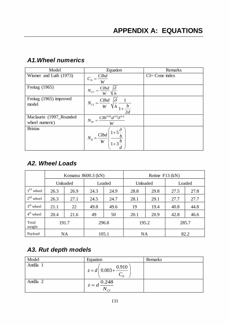
131

APPENDIX A: EQUATIONS

A1.Wheel numerics

Model Equation Remarks

Wismer and Luth (1973) N

CIbdC

W

CI= Cone index

Freitag (1965) CC

CIbdN

W h

Freitag (1965) improved

model 1

12

CI

CIbdN

bW h

d

Maclaurin (1997_Rounded

wheel numeric)

0.85 0.8 0.4

M

CIb dN

W

Brixius 1 5

1 3B

CIbd hNbW

d

A2. Wheel Loads

Komatsu 8600.3 (kN) Rottne F13 (kN)

Unloaded Loaded Unloaded Loaded

1ST

wheel 26.3 26.9 24.3 24.9 28.8 29.8 27.5 27.8

2nd

wheel 26.3 27.1 24.5 24.7 28.1 29.1 27.7 27.7

3rd

wheel 21.1 22 49.8 49.6 19 19.4 40.8 44.8

4th

wheel 20.4 21.6 49 50 20.1 20.9 42.8 46.6

Total

weight 191.7 296.8 195.2 285.7

Payload NA 105.1 NA 82.2

A3. Rut depth models


Antilla 1 0.9100.003

N

z dC

Antilla 2 0.248

CI

z dN

132

Antilla 3 0.3800.003

CC

zN

Antilla 4 0.3280.000

CI

zN

Antilla 5

1.2120.005

N

zC

Antilla 6

0.287

0.001CC

z dN

Antilla 7 0.2480.001

CI

z dN

Rantala 1 0.4900.059

CI

zN

Soft soil

Rantala 2

1.23

0.989

CI

zN

Soft soil

Rantala 3 0.6100.010

CI

zN

Saarilahti 1

0.83

0.142

CI

z dN

Maclaurin

1.25

0.224

CI

z dN

Gee-Glough 2

0.63 0.34

0.287

R

R

CI

dz

b

d

N

A4. Mobility models

Model Equation

Turnage (1972 b, WESFIELD) 1.310.8

2.45

0.200.04

2.50

P

CI

R

CI

N

N

Turnage (1972 a, WESLAB) 12.37

1.515.94

0.200.04

1.50

P

CI

R

CI

N

N

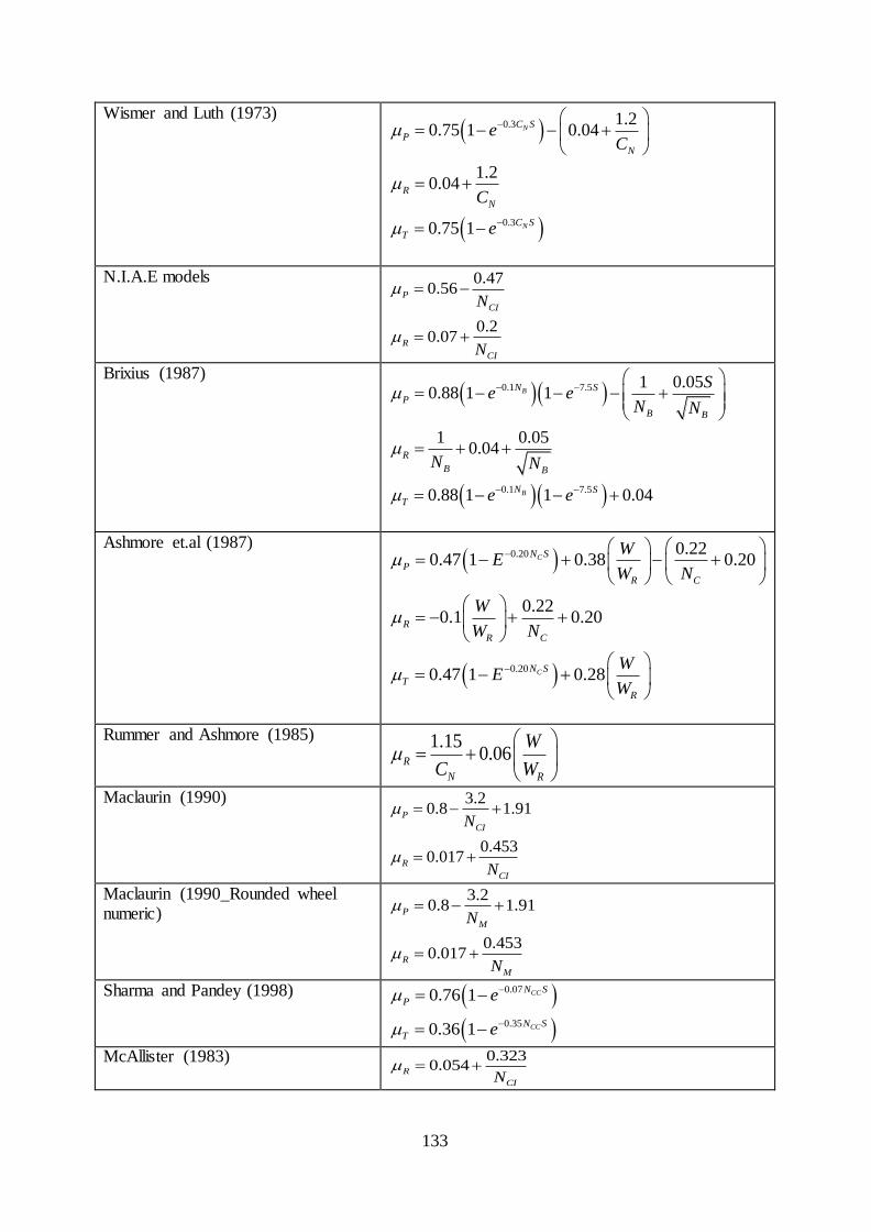
133

Wismer and Luth (1973)

0.3

0.3

1.20.75 1 0.04

1.20.04

0.75 1

N

N

C S

P

N

R

N

C S

T

eC

C

e

N.I.A.E models 0.47

0.56

0.20.07

P

CI

R

CI

N

N

Brixius (1987)

0.1 7.5

0.1 7.5

1 0.050.88 1 1

1 0.050.04

0.88 1 1 0.04

B

B

N S

P

B B

R

B B

N S

T

Se e

N N

N N

e e

Ashmore et.al (1987)

0.20

0.20

0.220.47 1 0.38 0.20

0.220.1 0.20

0.47 1 0.28

C

C

N S

P

R C

R

R C

N S

T

R

WE

W N

W

W N

WE

W

Rummer and Ashmore (1985) 1.150.06R

N R

W

C W

Maclaurin (1990) 3.2

0.8 1.91

0.4530.017

P

CI

R

CI

N

N

Maclaurin (1990_Rounded wheel numeric)

3.20.8 1.91

0.4530.017

P

M

R

M

N

N

Sharma and Pandey (1998)

0.07

0.35

0.76 1

0.36 1

CC

CC

N S

P

N S

T

e

e

McAllister (1983) 0.3230.054R

CIN

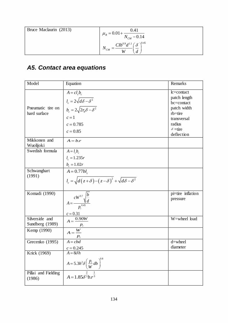
134


0.450.9 1.1

0.410.01

0.14R

CM

CM

N

CIb dN

W d

A5. Contact area equations


Pneumatic tire on

hard surface

2

2

2

2 2

1

0.785

0.85

c c

c

c b

A cl b

l d

b r

c

c

c

lc=contact

patch length bc=contact patch width

rb=tire transversal

radius =tire deflection

Mikkonen and Wuolijoki

.A b r

Swedish formula

1.235

1.02

c c

c

c

A l b

l r

b r

Schwanghart (1991)

2 2

0.77 c

c

A bl

l d z z d

Komadi (1990) 0.7

0.45

0.31

i

bcW

dA

p

c

pi=tire inflation pressure

Silverside and Sundberg (1989)

0.90

i

WA

p

W=wheel load

Kemp (1990)

i

WA

p

Grecenko (1995)

0.245

A cbd

c

d=wheel diameter

Krick (1969) 0.8

2

8

5.3 i

A h

pA h db

W

Pillai and Fielding

(1986)

2 1

3 31.85 .A b r

135

Godbole et al

(1993) 0.79

.0.54 i

A dh

p dhh

W

Dwyer (1984)

12

WA

G

W h bG

bd d

G=ground

pressure index

Febo (1987)

0.44

36

4

2

1

c c

c

c w

A l b

l d

b b e

Söhne (1969) 2A b dz z=sinkage

Diserns (2008)

5 5

5 5

0.1174 4.5 10 18.3 10

0.1360 6.7 10 32.2 10

i

i

A WD F P

A WD F P

WD=b X d

Keller (2005)

0.43 0.0006152 0.0022tyre tyre tyre wheelA w d p F

tyrew=tire with

tyred=tire

diameter

tyrep=tire

inflation pressure

wheelF= wheel

load

Duttmann (2012) 0.416. . 457.670 0.186.iA B D P F

F=wheel load

Lyasko (1994)

2

3

2

3

4

2

2.5

23

/ 3.5 11.9

p

p

A ab

a C Df f

b D f f

B HD

CD B

Diserns (2011) 0.2461.A TS

TS bd

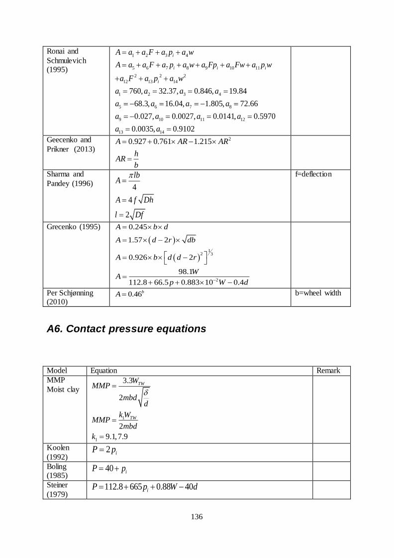
136

Ronai and

Schmulevich (1995)

1 2 3 4

5 6 7 8 9 10 11

2 2 2

12 13 14

1 2 3 4

5 6 7 8

9 10 11 12

13 14

760, 32.37, 0.846, 19.84

68.3, 16.04, 1.805, 72.66

0.027, 0.0027, 0.0141, 0.5970

0.0035, 0.

i

i i i

i

A a a F a p a w

A a a F a p a w a Fp a Fw a p w

a F a p a w

a a a a

a a a a

a a a a

a a

9102

Geecenko and

Prikner (2013)

20.927 0.761 1.215A AR AR

hAR

b

Sharma and

Pandey (1996) 4

4

2

lbA

A f Dh

l Df

f=deflection

Grecenko (1995)

1

2 3

2

0.245

1.57 2

0.926 2

98.1

112.8 66.5 0.883 10 0.4

A b d

A d r db

A b d d r

WA

p W d

Per Schjønning (2010)

0.46bA b=wheel width

A6. Contact pressure equations

Model Equation Remark

MMP

Moist clay

1

1

3.3

2

2

9.1,7.9

TW

TW

WMMP

mbdd

k WMMP

mbd

k

Koolen

(1992) 2 iP p

Boling (1985)

40 iP p

Steiner

(1979) 112.8 665 0.88 40iP p W d

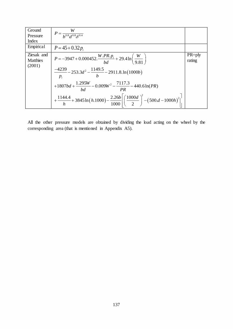
137

Ground

Pressure Index

0.8 0.8 0.4

WP

b d

Empirical 45 0.32 iP p

Ziesak and

Matthies (2001)

2

2

22

. .3947 0.000452. 29.4ln

9.81

4239 1149.5253.3 2911.8.ln 1000

1.295 7117.31807 0.009 440.6ln( )

1144.4 2.26 10003845ln .1000 500. 1000

1000 2

i

i

W PR p WP

bd

d bp b

Wbd W PR

bd PR

b dh d h

h

PR=ply

rating

All the other pressure models are obtained by dividing the load acting on the wheel by the

corresponding area (that is mentioned in Appendix A5).

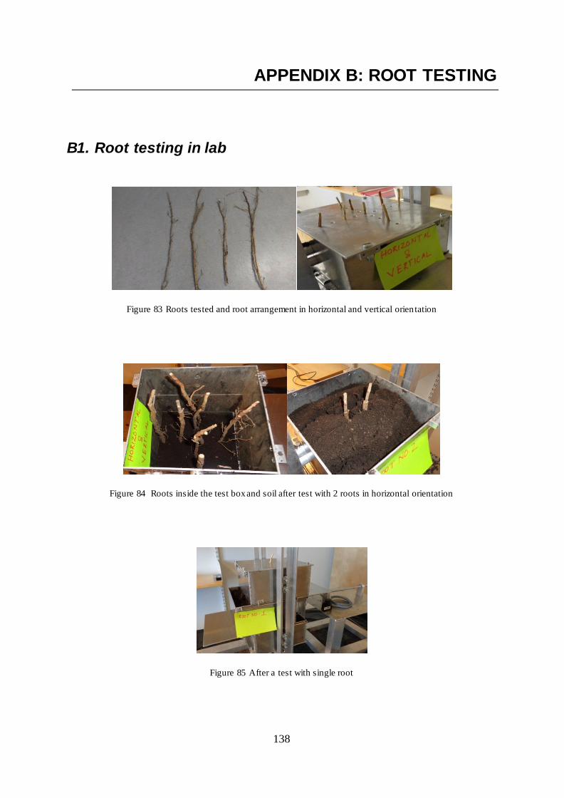
138

APPENDIX B: ROOT TESTING

B1. Root testing in lab

Figure 83 Roots tested and root arrangement in horizontal and vertical orientation

Figure 84 Roots inside the test box and soil after test with 2 roots in horizontal orientation

Figure 85 After a test with single root

139

APPENDIX C: DEPTH OF MEASUREMENT vs. CI

Figure 86 Depth of measurement vs. cone index for Komatsu and Komatsu with MAGNUM tracks

0

5

10

15

20

250.4 0.5 0.6 0.7 0.8 0.9 1 1.1 1.2 1.3

Depth

of

measure

ment

in c

m


Komatsu Loaded 450 kPa

After 1st pass

After 5th pass

After 10th pass

0

5

10

15

20

250.2 0.4 0.6 0.8 1 1.2 1.4 1.6

Depth

of

measure

ment

in c

m


Komatsu MAGNUM

After 1st pass

After 10th pass

140

APPENDIX D: DIRECT SHEAR TEST RESULT

Figure 87 Result of direct shear test of the soil

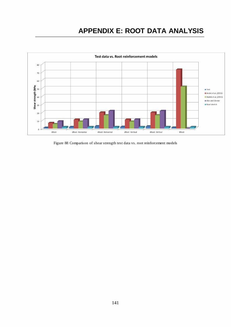
141

APPENDIX E: ROOT DATA ANALYSIS

Figure 88 Comparison of shear strength test data vs. root reinforcement models

Tire-soil interaction analysis of forest machines Karthik ...

Documents

Transcript of Tire-soil interaction analysis of forest machines Karthik ...