Tiny ImageNet Challenge

Anna ShcherbinaStanford University

annashch@stanford.edu

Abstract

An ensemble of three convolutional network architec-tures was used to classify 10,000 images from the Tiny Im-ageNet challenge into 200 distinct classes. A test error rateof 0.506 was achieved. The top single model in the ensem-ble achieves an error rate of 0.524. The top-performingarchitecture was a keras implementation of the VGG-16 ar-chitecture. To avoid overfitting to the training data, the datawas augmented through image rotation, cropping, and colorjitter. Additionally, dropout and regularization (L1 and L2)were utilized. Network performance was further analyzedby visualization of the filters, computation of saliency maps,and determining the per-class distribution of the model val-idation accuracy.

1. IntroductionImage classification is a fundamental problem in com-

puter vision. The ImageNet Challenge[14] tasks par-ticipants with classifying 100,000 test images into 1000classes, giving a training set of 1.2 million images. Top-1 and top-5 accuracy on the test dataset is used to rankperformance. The Tiny ImageNet Challenge follows thesame principle, though on a smaller scale – the images aresmaller in dimension (64x64 pixels, as opposed to 256x256pixels in standard ImageNet) and the dataset sizes are lessoverwhelming (100,000 training images across 200 classes;10,000 test images).

Since the ImageNet Challenge was first held in 2010, adeep learning revolution has occurred in computer vision.Initial winners of the challenge relied on standard tech-niques in computer vision. In this approach feature suchas SIFT [12], histogram of gradients [6], and local binarypatterns [13] must be extracted from the training data andpooled for a global image representation using techniquessuch as spatial pyramid matching[11] and Fisher vector rep-resentation [7]. The pooled features are then input to a clas-sifier such as a support vector machine to perform the imageclassification. These approaches work well on the scale ofthousands or tens of thousands of images but do not scale

efficiently for the 1.2 million images in ImageNet.Convolutional neural networks help to overcome the lim-

itations of traditional classification techniques. They do notrequire pre-defined input features, but rather learn them aspart of the training process. Furthermore, the convolutionand dot product operations of ConvNets can be highly vec-torized, which allows for highly parallel and fast GPU im-plementation. The high suitability of convolutional neuralnetworks for image classification is illustrated by the suc-cess of Krizhevsky et al [9], Szegedy et al [18] in applyingthese techniques to win the ImageNet Challenge.

In this project, I experiment with four convolutional neu-ral network architectures to classify the images in the TinyImageNet Challenge. Pretrained weights are used whenavailable; otherwise networks are trained from scratch. I fo-cus on adding dropout, regularization, and data augmenta-tion to prevent models from overfitting on the training data.Several approaches are implemented to visualize model per-formance and to identify classes where the model achieveshigh accuracy, as well as classes where the model performspoorly.

2. MethodsAll models for this project were implemented in Python

using the Keras library (v1.3)[5] running on top of Theano(v.0.7)[4]. All code and network weights for the project canbe downloaded from Github: https://github.com/annashcherbina/cs231n_project.git.

The image data was pre-processed by calculating the per-channel mean of the training data and subtracting this valuefrom each image in the training, validation, and test data.The dataset pixel values were subsequently normalized viadivision by the per-channel standard deviation of the train-ing dataset. The skimage Python library was used for dataloading and pre-processing[19].

2.1. Data augmentation

The training dataset provides 50 images for each of 200classes, for a total of 100,000 images. Data augmentationwas used to increase the amount of available training data.Five augmentation steps were performed (Figure 1). Images

1

Figure 1. Data augmentation approaches that were applied to thetraining data.Images were flipped horizontally, flipped vertically,cropped, color-contrasted, and tinted.

were flipped about the vertical axis or about the horizontalaxis. Random crops of 55x55 pixels were extracted fromimages, and the resulting smaller image was then scaled(via spline interpolation) to the original size of 64x64 pix-els. The scaling was done with the resize function in theskimage library. Image contrast was adjusted randomly. Foreach input image in the training data, a number from therange [0.8,1.2] was selected at random, and each pixel of theimage was multiplied by that number. Images were tintedat random. For each input image, a random color was gen-erated whose red, green, and blue components were drawnuniformly at random from the range (-5,5). This color wasadded to each pixel of the image. Augmenting each imagewith all five techniques would have increased the trainingdata size by 500%, which is too large to fit in memory formy available system. Consequently, 30% of the trainingdata was selected at random for each of the augmentations,yielding a total training set size of 265,000 images.

2.2. Network architectures

Four ConvNet architectures were trained on the Tiny Im-ageNet dataset. These are illustrated in Figure 2.

2.2.1 Nine-layer network from CS231n assignment 3

The nine-layer network from assignment three was selecteddue to the availability of pretrained weights (Figure 2a).All convolution layer parameters were identical to val-ues used in assignment 3. For the spatial batch normal-ization, the default Keras parameters were utilized (ε=1e-6,momentum=0.9). To reduce overfitting, the network wasmodified by adding 0.25 dropout after the third convolutionlayer, 0.25 dropout after the sixth convolution layer, and0.5 dropout after each of the fully-connected layers[17]. L1

and L2 regularization was also added as a further step to re-duce overfitting. The first convolutional layer was weaklyregularized (L1 λ=1e-7, L2 λ= 1e-7). Stronger regulariza-tion was applied to each of the dense layers: L1 λ=1e-5, L2λ=1e-5.

The network was trained via stochastic gradient descentfor a total of 17 epochs. It was found that training for morethan 17 epochs caused the validation accuracy to decrease(Figure 4), potentially a consequence of the network over-shooting the global minimum. Learning rates of 1e-7, 1e-5,1e-3, 1e-1, 5e-1 were utilized, and it was found that the net-work converged to the highest final accuracy with a learn-ing rate of 1e-1. The default SGD parameters in Keras weretried (decay=1e-6, Nesterov momentum=0.9), but the net-work did not converge when these were applied. Removingdecay and Nesterov momentum led to the highest validationaccuracy and the fastest convergence time.

2.2.2 VGG-like network

The network illustrated in Figure 2b was provided as an ex-ample in the Keras documentation, and I used it for two pur-poses: to ensure that my Keras setup was working properly,and to learn the quality of results that could be obtainedby training a network from scratch, as opposed to begin-ning with pre-trained weights. This was done because nopretrained weights were available for this network, whichis a simplification of the VGG-16 network. In contrast toVGG-16, the VGG-like network utilizes only 4 convolua-tion layers. I modified the original network in [5] by adding0.25 dropout after the second and fourth convolution layers,as well as 0.5 dropout after the first dense layer. To furtherreduce dropout, L1 and L2 regularization was added to thedense layers (L1 and L2 λ=1e-6 for the first dense layer; L1and L2 λ=1e-5 for the second dense layer). The networkwas trained via stochastic gradient descent with learningrate 1e-1 for a total of 30 epochs (until validation accuracyplateaued).

2.2.3 VGG-16

The VGG-16 architecture described in [16] was imple-mented in Keras (Figure 2c.) Pre-trained weights for thearchitecture were downloaded from [1]. Because the orig-inal architecture was trained on the ImageNet dataset with1000 output classes, the pre-trained weights for the Denselayers could not be used due to dimension mismatch. Con-sequently, the weights for the dense layers were initializedusing the Glorot initialization [8]. The original VGG-16 ar-chitecture was modified by increasing dropout to 0.75 afterthe first and second fully-connected layers (as compared to0.5 in the original architecture). This was done to mitigatethe overfitting problem. L1 and L2 regularization was alsoadded to the original VGG16 architecture to further reduce

Figure 2. Four network architectures were trained as part of this project. a. Nine-layer ConvNet from Assignment 3. b. SimplifiedVGG-like network. c. VGG-16. d. AlexNet.

overfitting. Both weight regularization and activity regular-ization were added, and regularization parameters increaseddeeper into the network, however experiments showed thatincreased the regularization λ beyond 1e-4 prevented thenetwork from learning, while using λ lower than 1e-7 was

insufficient to have any meaningful effect on overfitting,leading to the following final set of regularization param-eters:

• Conv Layer 11: L1 λ=1e-7, L2 λ=1e-7

• Conv Layer 12: L1 λ=1e-6, L2 λ=1e-6

• Conv Layer 13: L1 λ=1e-5, L2 λ=1e-5

• Dense Layer 1: L1 λ=1e-4, L2 λ=1e-5

• Dense Layer 2: L1 λ=1e-4, L2 λ=1e-4

The network was trained via stochastic gradient descent for6 epochs, since the validation accuracy plateaued at thistime, and training for additional epochs had no effect. Ex-perimentation with learning rates of (1e-7, 1e-5, 1e-3, 1e-1) indicated optimal validation accuracy and faster conver-gence for a learning rate of 1e-3. For the VGG-16 model,the default Keras SGD parameters (decaye=1e-6, Nesterovmomentum=0.9) did work better than SGD without theseoptimizations (in contrast to the 9-layer ConvNet describedabove).

2.2.4 AlexNet

I attempted to implement the AlexNet architecture[9] inKeras. The implementation is illustrated in Figure 2d. How-ever, I was not able to evaluate this architecture because thememory required to run it was greater than that available onmy computer system. This is due to the fact that AlexNet isa much wider architecture than VGG and the 9-layer Con-vNet,though it is not as deep and utilizes only 4 convolu-tional layers. Experiments to replace the first convolutionallayer of size (64x11x11) with smaller layers (64x9x9) or(64x7x7) continued to yield memory errors, preventing mefrom being able to evaluate the performance of this archi-tecture.

2.2.5 Ensemble of architecture results

A majority vote of the three trained models was taken. Ifall three models disagreed, the VGG-16 class label was as-signed, since that is the model with the highest validationaccuracy. Pearson correlation was calculated to determinethe degree of correlation in validation error rates across themodels.

2.3. Optimization and Experimentation

2.3.1 Individual pre-training of layers

As an attempt to improve accuracy, layers in the 9-layerConvNet were pretrained individually. Initially, the learn-ing rate for all layers except the first convolutional layerwas set to 0. Once that layer had been trained, the learningrate for the second convolutional layer was set to the de-fault value (1e-1). The learning rate for the first layer waskept at 1e-1 to allow this layer to continue learning in thecontext of the full network as additional layers were added.

Figure 3. Accuracy and loss for the 9-layer ConvNet architecturewith convolutional layers pre-trained individually.

In this manner, all remaining convolutional and dense lay-ers were pre-trained and stacked on top of the previous lay-ers. This approach follows one of the methods described byLarochelle et al [10]. The training accuracy and loss for thisapproach are illustrated in Figure 3. An accuracy of 98% isachieved on the training data, but the approach also suffersfrom sever overfitting, as illustrated by the 7.6% accuracyon the test dataset and 3.80% accuracy on the validationdataset (Table 1). Although these metrics were calculatedprior to the addition of dropout and regularization, the per-formance was poor enough such that this approach was notutilized in the final set of models.

Loss AccuracyTraining 0.135 0.983Validation 7.629 0.038Test 0.0760

Table 1. Training, validation, and test accuracy of the 9-layer Con-vNet architecture with convolutional layers pre-trained individu-ally.

3. Results

3.1. Tiny ImageNet Classification Error

An error rate of 0.506 was attained on the Tiny ImageNettest dataset. The individual performance of the three net-work architectures illustrated in Figure2 is summarized inTable 2. The VGG-16 architecture achieved a test accu-racy of 0.494, while the Assignment 3 ConvNet achievedan accuracy of 0.423, and the simpler VGG-like networkachieved an accuracy of 0.237. Interestingly, a majorityvote of the architectures achieved an accuracy of 0.492 per-cent, slightly lower than that of the VGG-16 architecture.This is due to the fact that the errors across the three archi-

tectures are highly correlated (Pearson correlation = 0.732),so we do not get the expected 2% accuracy boost from anensemble classifier.

Architecture TrainingAccuracy

ValidationAccu-racy

Test Ac-curacy

9-Layer ConvNet 0.988 0.455 0.423VGG-like ConvNet 0.488 0.288 0.237VGG-16 0.760 0.535 0.494Ensemble 0.492

Table 2. Accuracy of the three network architectures on Tiny Ima-geNet training, validation, and test datasets.

The change in loss and accuracy over epochs of trainingis illustrated in Figure4.

3.2. Model Visualization

3.2.1 Saliency Maps

A function was implemented to compute saliency mapsin accordance with Simonyan et al[15] and Zeiler [21].Saliency maps for each of the 3 models on a test image fromclass n07768694 (”pomegranite”) are illustrated in Figure5.All three classifiers classified this image correctly. The ab-solute value of the saliency score is illustrated in gray scale,while areas of positive and negative saliency are shaded incolor. The saliency maps for the three maps are different,but they are not readily interpretable.

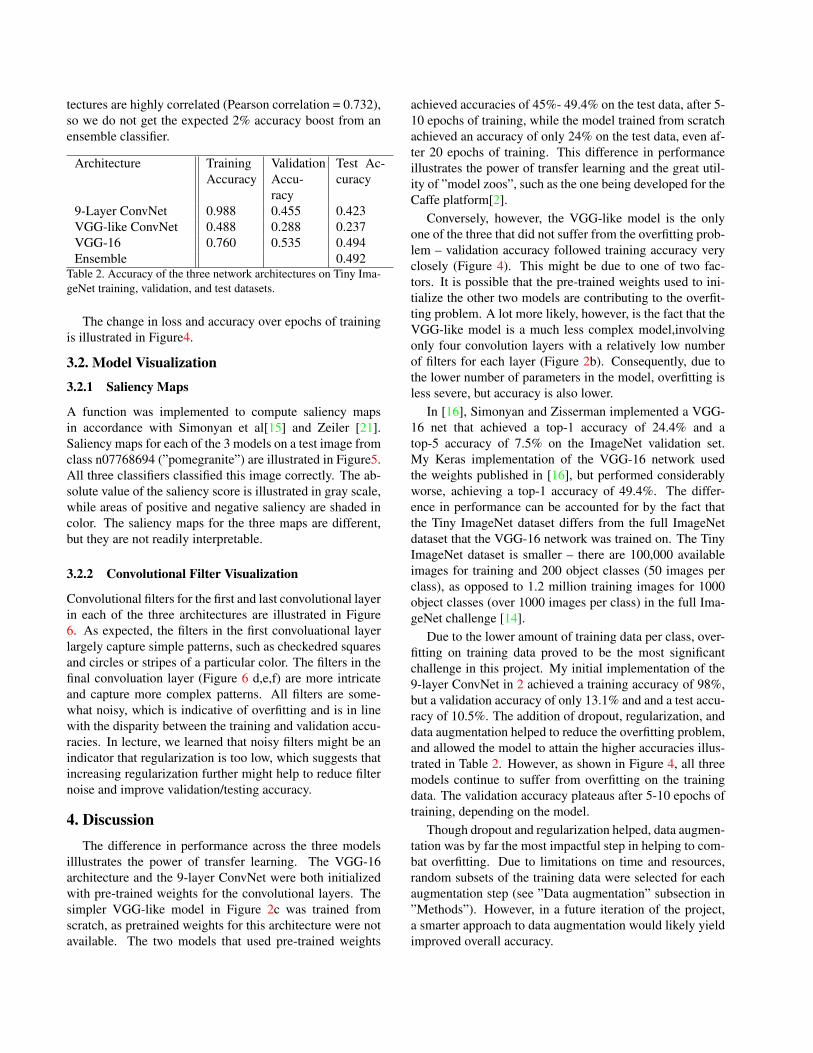
3.2.2 Convolutional Filter Visualization

Convolutional filters for the first and last convolutional layerin each of the three architectures are illustrated in Figure6. As expected, the filters in the first convoluational layerlargely capture simple patterns, such as checkedred squaresand circles or stripes of a particular color. The filters in thefinal convoluation layer (Figure 6 d,e,f) are more intricateand capture more complex patterns. All filters are some-what noisy, which is indicative of overfitting and is in linewith the disparity between the training and validation accu-racies. In lecture, we learned that noisy filters might be anindicator that regularization is too low, which suggests thatincreasing regularization further might help to reduce filternoise and improve validation/testing accuracy.

4. DiscussionThe difference in performance across the three models

illlustrates the power of transfer learning. The VGG-16architecture and the 9-layer ConvNet were both initializedwith pre-trained weights for the convolutional layers. Thesimpler VGG-like model in Figure 2c was trained fromscratch, as pretrained weights for this architecture were notavailable. The two models that used pre-trained weights

achieved accuracies of 45%- 49.4% on the test data, after 5-10 epochs of training, while the model trained from scratchachieved an accuracy of only 24% on the test data, even af-ter 20 epochs of training. This difference in performanceillustrates the power of transfer learning and the great util-ity of ”model zoos”, such as the one being developed for theCaffe platform[2].

Conversely, however, the VGG-like model is the onlyone of the three that did not suffer from the overfitting prob-lem – validation accuracy followed training accuracy veryclosely (Figure 4). This might be due to one of two fac-tors. It is possible that the pre-trained weights used to ini-tialize the other two models are contributing to the overfit-ting problem. A lot more likely, however, is the fact that theVGG-like model is a much less complex model,involvingonly four convolution layers with a relatively low numberof filters for each layer (Figure 2b). Consequently, due tothe lower number of parameters in the model, overfitting isless severe, but accuracy is also lower.

In [16], Simonyan and Zisserman implemented a VGG-16 net that achieved a top-1 accuracy of 24.4% and atop-5 accuracy of 7.5% on the ImageNet validation set.My Keras implementation of the VGG-16 network usedthe weights published in [16], but performed considerablyworse, achieving a top-1 accuracy of 49.4%. The differ-ence in performance can be accounted for by the fact thatthe Tiny ImageNet dataset differs from the full ImageNetdataset that the VGG-16 network was trained on. The TinyImageNet dataset is smaller – there are 100,000 availableimages for training and 200 object classes (50 images perclass), as opposed to 1.2 million training images for 1000object classes (over 1000 images per class) in the full Ima-geNet challenge [14].

Due to the lower amount of training data per class, over-fitting on training data proved to be the most significantchallenge in this project. My initial implementation of the9-layer ConvNet in 2 achieved a training accuracy of 98%,but a validation accuracy of only 13.1% and and a test accu-racy of 10.5%. The addition of dropout, regularization, anddata augmentation helped to reduce the overfitting problem,and allowed the model to attain the higher accuracies illus-trated in Table 2. However, as shown in Figure 4, all threemodels continue to suffer from overfitting on the trainingdata. The validation accuracy plateaus after 5-10 epochs oftraining, depending on the model.

Though dropout and regularization helped, data augmen-tation was by far the most impactful step in helping to com-bat overfitting. Due to limitations on time and resources,random subsets of the training data were selected for eachaugmentation step (see ”Data augmentation” subsection in”Methods”). However, in a future iteration of the project,a smarter approach to data augmentation would likely yieldimproved overall accuracy.

Figure 4. Accuracy and loss for the three network architectures that were trained in this project. The red line indicates training accuracyand loss; the blue line indicates validation accuracy and loss.

Specifically, examination of error by object class illus-trates that the model is much better at identifying some ob-ject classes than others. For example, as shown in Table 3,the model does exceptionally well at identifying goldfish,school buses, trains, monarch butterflies and ladybugs. Thisfinding is un-surprising – these image classes are all quitedistinct from other image classes, and quite homogeneouswithin themselves. For example, Figure 7a illustrates thatthe goldfish images used in the validation dataset are fairlystandard – the fish is center stage and the shape/colorationof the object remains consistent. The model had moretrouble with objects of class umbrella, punch bag, woodenspoon, syringe, and plunger. As illustrated in Figure 7b,many of the problem images have multiple objects otherthan the object of interest. The object of interest is small,off -center, or portrayed from an unusual angle. These failcases are in line with those described by Karpathy in [3] (i.e.small, thin objects such as the syringe or wooden spoon).

Class Label Words NumberMisclas-sified

n01443537 goldfish 4n04146614 school bus 6n02917067 bullet train 7n02279972 monarch butterfly 8n02165456 ladybug 8n04507155 umbrella 39n04023962 punch bag 39n04597913 wooden spoon 39n04376876 syringe 41n03970156 plunger 42

Table 3. Number of images that were misclassified in the valida-tion dataset by VGG-16. The top portion of the table illustratesthe 5 classes with the highest overall accuracy; the bottom portionillustrates the 5 classes with the lowest overall accuracy.

Figure 5. Saliency maps for test image test 8715.JPEG. a) Originalimage. b) Preprocessed image. Mean has been subtracted andimage has been normalized by standard deviation of training data.c) Saliency maps from the 9-layer ConvNet model; absolute valuein grayscale, followed by positive saliency and negative saliency.d) Saliency maps from the VGG-16 model. e) Saliency maps fromthe VGG-like model.

5. Future WorkThe biggest obstacle to high classification accuracy for

the Tiny ImageNet challenge is overfitting – accuracy of98% can be achieved on the training data with the pre-trained VGG16 and 9-layer ConvNet models, but validationaccuracy plateaus at approximately 50%. Consequently, fu-ture work will focus on reducing the overfitting problem.Some techniques that may be of use include:

• I attempted to implement DropConnect[20] for theproject, but unfortunately ran out of time. Whereasdropout sets a random subsets of activations in eachlayer to zero, DropConnect sets a random subset ofweights to zero. This causes each unit to receive inputsfrom a random subset of units in the preceding layer,further increasing noise in the system, and helping toreduce overfitting.

• Smart data augmentation could also mitigate the over-

Figure 6. Convolutional filter visualization. a) 9-layer ConvNet,first convolutional layer. b) VGG-16, first convolutional layer. c)VGG-like ConvNet, first convolutional layer. d) 9-layer ConvNet,ninth convolutional layer. e) VGG-16, 13th convolutional layer. f)VGG-like ConvNet, fourth convolutional layer.

Figure 7. Representative images from the image classes in the val-idation dataset with best and worst accuracy. a) The ”goldfish”class had the highest accuracy. b) The ”plunger” class had thelowest accuracy.

fitting problem. Currently, 30% of training images areselected at random to undergo each of the augmenta-tions. However, as described in the Discussion sec-tion, some object classes are a lot easier to identifythan others. Based on the initial results from the VGG-16 model, I would like to further augment the imageclasses where the model had the lowest accuracy (Ta-ble 3).

• I found that the time it takes to train the networks poseda bottleneck to development and iteration. To reducethe training time, I would like to prune redundant con-nections in the network, as described by Song Han et

al in [15]. In a first pass on the training data the im-portant connections will be learned. Low-weight con-nections will then be pruned. Finally, the network willbe retrained to learn the weights for the surviving con-nections.

References[1] https://gist.github.com/baraldilorenzo/

07d7802847aaad0a35d3. 2[2] http://caffe.berkeleyvision.org/model_

zoo.html. 5[3] http://karpathy.github.io/2014/09/02/

what-i-learned-from-competing-against-a-convnet-on-imagenet/.6

[4] J. Bergstra, O. Breuleux, F. Bastien, P. Lamblin, R. Pascanu,G. Desjardins, J. Turian, D. Warde-Farley, and Y. Bengio.Theano: a CPU and GPU math expression compiler. In Pro-ceedings of the Python for Scientific Computing Conference(SciPy), June 2010. Oral Presentation. 1

[5] F. Chollet. Keras. https://github.com/fchollet/keras, 2015. 1, 2

[6] N. Dalal and B. Triggs. Histograms of oriented gradients forhuman detection. In Proceedings of the 2005 IEEE Com-puter Society Conference on Computer Vision and PatternRecognition (CVPR’05) - Volume 1 - Volume 01, CVPR ’05,pages 886–893, Washington, DC, USA, 2005. IEEE Com-puter Society. 1

[7] V. Garg, S. Chandra, and C. V. Jawahar. Sparse discrimina-tive fisher vectors in visual classification. In Proceedings ofthe Eighth Indian Conference on Computer Vision, Graphicsand Image Processing, ICVGIP ’12, pages 55:1–55:8, NewYork, NY, USA, 2012. ACM. 1

[8] X. Glorot and Y. Bengio. Understanding the difficultyof training deep feedforward neural networks. In JMLRW&CP: Proceedings of the Thirteenth International Confer-ence on Artificial Intelligence and Statistics (AISTATS 2010),volume 9, pages 249–256, May 2010. 2

[9] A. Krizhevsky, I. Sutskever, and G. E. Hinton. Imagenetclassification with deep convolutional neural networks. InF. Pereira, C. J. C. Burges, L. Bottou, and K. Q. Weinberger,editors, Advances in Neural Information Processing Systems25, pages 1097–1105. Curran Associates, Inc., 2012. 1, 4

[10] H. Larochelle, Y. Bengio, J. Louradour, and P. Lamblin. Ex-ploring strategies for training deep neural networks. Journalof Machine Learning Research, 10:1–40, 2009. 4

[11] S. Lazebnik, C. Schmid, and J. Ponce. Beyond bags offeatures: Spatial pyramid matching for recognizing naturalscene categories. In Proceedings of the 2006 IEEE ComputerSociety Conference on Computer Vision and Pattern Recog-nition - Volume 2, CVPR ’06, pages 2169–2178, Washing-ton, DC, USA, 2006. IEEE Computer Society. 1

[12] D. G. Lowe. Distinctive image features from scale-invariantkeypoints. Int. J. Comput. Vision, 60(2):91–110, Nov. 2004.1

[13] M. Pietikainen, A. Hadid, G. Zhao, and T. Ahonen. Com-puter Vision Using Local Binary Patterns, volume 40.Springer, 2011. 1

[14] O. Russakovsky, J. Deng, H. Su, J. Krause, S. Satheesh,S. Ma, Z. Huang, A. Karpathy, A. Khosla, M. Bernstein,A. C. Berg, and L. Fei-Fei. ImageNet Large Scale VisualRecognition Challenge. International Journal of ComputerVision (IJCV), 115(3):211–252, 2015. 1, 5

[15] K. Simonyan, A. Vedaldi, and A. Zisserman. Deep in-side convolutional networks: Visualising image classifica-tion models and saliency maps. CoRR, abs/1312.6034, 2013.5, 8

[16] K. Simonyan and A. Zisserman. Very deep convolu-tional networks for large-scale image recognition. CoRR,abs/1409.1556, 2014. 2, 5

[17] N. Srivastava, G. Hinton, A. Krizhevsky, I. Sutskever, andR. Salakhutdinov. Dropout: A simple way to prevent neu-ral networks from overfitting. Journal of Machine LearningResearch, 15:1929–1958, 2014. 2

[18] C. Szegedy, W. Liu, Y. Jia, P. Sermanet, S. Reed,D. Anguelov, D. Erhan, V. Vanhoucke, and A. Rabinovich.Going deeper with convolutions. CoRR, abs/1409.4842,2014. 1

[19] S. van der Walt, J. L. Schonberger, J. Nunez-Iglesias,F. Boulogne, J. D. Warner, N. Yager, E. Gouillart, T. Yu,and the scikit-image contributors. scikit-image: image pro-cessing in Python. PeerJ, 2:e453, 6 2014. 1

[20] L. Wan, M. Zeiler, S. Zhang, Y. L. Cun, and R. Fergus. Reg-ularization of neural networks using dropconnect. In S. Das-gupta and D. Mcallester, editors, Proceedings of the 30thInternational Conference on Machine Learning (ICML-13),volume 28, pages 1058–1066. JMLR Workshop and Confer-ence Proceedings, May 2013. 7

[21] M. D. Zeiler and R. Fergus. Visualizing and understandingconvolutional networks. CoRR, abs/1311.2901, 2013. 5