Using Explanatory Item Response Models to Evaluate Complex Scientific Tasks Designed for

the Next Generation Science Standards

by

Tina Chiu

A dissertation submitted in partial satisfaction of the

requirements for the degree of

Doctor of Philosophy

in

Education

in the

Graduate Division

of the

University of California, Berkeley

Committee in charge:

Professor Mark Wilson, Chair

Professor P. David Pearson

Professor Jonathan Osborne

Professor Nicholas P Jewell

Spring 2016

1

Abstract

Using Explanatory Item Response Models to Evaluate Complex Scientific Tasks Designed for

the Next Generation Science Standards

by

Tina Chiu

Doctor of Philosophy in Education

University of California, Berkeley

Professor Mark Wilson, Chair

This dissertation includes three studies that analyze a new set of assessment tasks

developed by the Learning Progressions in Middle School Science (LPS) Project. These

assessment tasks were designed to measure science content knowledge on the structure of matter

domain and scientific argumentation, while following the goals from the Next Generation Science

Standards (NGSS). The three studies focus on the evidence available for the success of this design

and its implementation, generally labelled as “validity” evidence. I use explanatory item response

models (EIRMs) as the overarching framework to investigate these assessment tasks. These

models can be useful when gathering validity evidence for assessments as they can help explain

student learning and group differences.

In the first study, I explore the dimensionality of the LPS assessment by comparing the fit

of unidimensional, between-item multidimensional, and Rasch testlet models to see which is most

appropriate for this data. By applying multidimensional item response models, multiple

relationships can be investigated, and in turn, allow for a more substantive look into the assessment

tasks. The second study focuses on person predictors through latent regression and differential

item functioning (DIF) models. Latent regression models show the influence of certain person

characteristics on item responses, while DIF models test whether one group is differentially

affected by specific assessment items, after conditioning on latent ability. Finally, the last study

applies the linear logistic test model (LLTM) to investigate whether item features can help explain

differences in item difficulties.

i

For my mother

ii

Table of Contents

List of Figures iv

List of Tables v

1 Introduction 1

1.1 Background and Motivation ……………………………………………... 1

1.1.1 Validity Evidence and Assessments ……………………………... 1

1.1.2 The Next Generation Science Standards (NGSS) ………………... 2

1.2 The Learning Progressions in Middle School Science (LPS) Project …… 3

1.2.1 The Structure of Matter Learning Progression and the Particulate

Explanations of Physical Changes (EPC) Construct …………….. 3

1.2.2 The Scientific Argumentation Learning Progression ……………. 6

1.2.3 Complex Tasks for 2013-2014 Data Collection …………………. 9

1.2.4 2013-2014 Data: The Students …………………………………... 11

1.3 The Three Research Areas ………………………………………………. 14

1.3.1 Model Selection and Software …………………………………... 14

2 Multidimensional Modeling of the Complex Tasks 16

2.1 Introduction ……………………………………………………………… 16

2.2 Unidimensional, Between-item Multidimensional, and Testlet Models … 17

2.3 Results …………………………………………………………………… 23

2.3.1 Between-item Multidimensional Model Results ………………… 23

2.3.2 Testlet Models Results …………………………………………… 29

2.3.3 Model Selection ………………………………………………….. 33

2.4 Discussion and Future Steps ……………………………………………... 35

3 Person Regression Models and Person-by-item Models for Explaining

Complex Tasks 36

3.1 Introduction ………………………………………………………………. 36

3.1.1 Test Fairness ……………………………………………………… 36

3.1.2 Research Questions ………………………………………………. 37

3.1.3 Note on the Sample ………………………………………………. 37

3.2 Explanatory Item Response Models for Person Predictors and Person-by-

Item Predictors …………………………………………………………… 38

3.2.1 Multidimensional Latent Regression …………………………….. 38

3.2.2 Differential Item Functioning (DIF) ……………………………... 39

3.3 Results ……………………………………………………………………. 41

iii

3.3.1 Latent Regression Results ………………………………………... 41

3.3.2 Post-hoc DIF Results: EL Proficiency …………………………… 45

3.3.3 DIF Results: Gender ……………………………………………… 46

3.4 Discussion and Future Steps ……………………………………………… 50

4 Exploring the Item Features of the Complex Tasks 52

4.1 Introduction ………………………………………………………………. 52

4.1.1 Item Features for the Complex Tasks ……………………………. 52

4.1.2 Research Questions ………………………………………………. 55

4.2 Explanatory Item Response Models for Item Features …………………... 56

4.2.1 The Linear Logistic Test Model and Its Extensions ……………… 56

4.3 Results ……………………………………………………………………. 57

4.3.1 Descriptive Statistics ……………………………………………... 57

4.3.2 Research Question 4: LLTM Results …………………………….. 59

4.3.3 Research Question 5: LLTM with Interaction Results …………... 62

4.3.4 Model Comparisons ……………………………………………… 66

4.4 Discussion and Future Steps ……………………………………………... 68

References ……………………………………………………………………………….. 69

iv

List of Figures

1.1 Structure of matter learning progression from the Learning Progressions in

Science (LPS) Project ……………………………………………………………. 4

1.2 Construct map for Particulate Explanations of Physical Changes (EPC) ………… 5

1.3 Argumentation learning progression from the LPS project ……………….. ……. 7

1.4 An example of an argumentation item from the Onions complex task ………….. 10

1.5 An example of an embedded content item from the Onions complex task ……… 10

1.6 An example of a content item from the Onions complex task …………………… 11

2.1 Diagram for the unidimensional model …………………………………………... 18

2.2 Diagram for the two-dimensional between-item model ………………………….. 19

2.3 Diagram for the three-dimensional between-item model ………………………… 20

2.4 Diagram for the testlet model with one underlying dimension …………………... 21

2.5 Diagram for the testlet model with two underlying dimensions …………………. 22

2.6 Wright map for the three-dimensional between-item model, after DDA ………… 28

2.7 Wright map for two-dimensional testlet model. Only content and embedded items

are plotted ……………………………………………………………………….... 32

3.1 Number of Reclassified, Fluent, and English Only students at each ability

estimate for the argumentation dimension ……………………………………….. 44

3.2 Number of Reclassified, Fluent, and English Only students at each ability

estimate for the embedded content dimension …………………………………… 44

3.3 Number of Reclassified, Fluent, and English Only students at each ability

estimate for the content dimension ……………………………………………… 45

3.4 An argumentation item flagged as having statistically significant DIF …………. 47

3.5 Item characteristic curves for male and female students for argumentation item

in Figure 3.4 ……………………………………………………………………… 48

4.1 A LPS item with a schematic representation …………………………………….. 53

4.2 A LPS item with a pictorial representation ………………………………………. 54

4.3 A LPS item with no pictures ……………………………………………………... 54

4.4 Wright map showing item parameter estimates (from partial credit model) by

multiple-choice and open-ended items ………………………………………….. 61

4.5 The academic words on the LPS test and the corresponding item type …………. 64

4.6 Graph of step difficulties estimated from partial credit model with those

estimated from the LLTM ……………………………………………………….. 67

4.7 Graph of step difficulties estimated from partial credit model with those

estimated from the LLTM with interactions …………………………………….. 67

v

List of Tables

1.1 Distribution of types of items across the three complex tasks …………………… 11

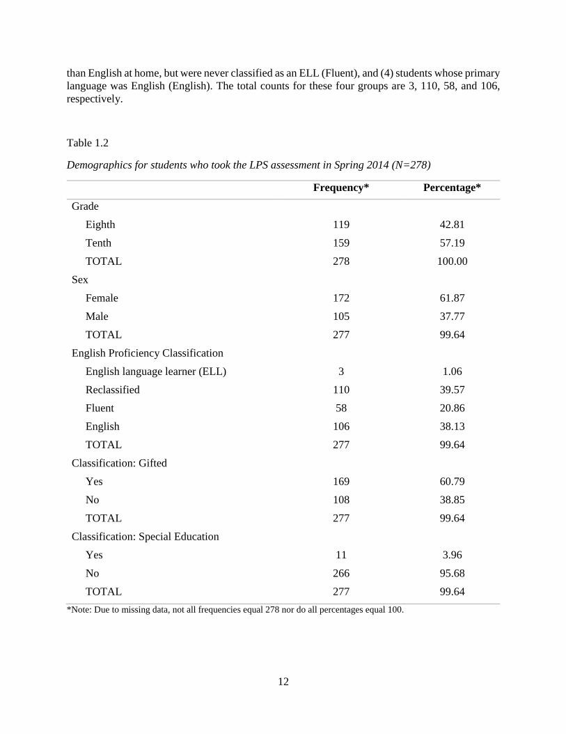
1.2 Demographics for students who took the LPS assessment in Spring 2014 ……… 12

1.3 Summary statistics for students who took the LPS assessment in Spring 2014 …. 13

1.4 Frequency and percentage of students’ performance on state science test by

grade ……………………………………………………………………………… 13

2.1 Results for the two-dimensional between-item model ………………………….... 24

2.2 Results for the three-dimensional between-item model ………………………….. 24

2.3 Correlation table for the three-dimensional between-item model ……………....... 24

2.4 Results for three-dimensional between-item model, after DDA …………………. 26

2.5 Results for the two-dimensional testlet model ……………………………………. 30

2.6 Variance in the two-dimensional between-item and testlet models with one and

two dimensions ……………………………………………………………………. 30

2.7 Results for the unidimensional, two- and three-dimensional between-item models

and testlet models ………………………………………………………………… 34

3.1 Multidimensional latent regression results ………………………………………. 42

3.2 Post-hoc comparisons for students classified as Fluent and Reclassified ……….. 43

3.3 Breakdown of responses to flagged item by gender and estimated ability in

Argumentation …………………………………………………………………… 49

4.1 Frequencies for Each Item Feature on the LPS Assessment …………………….. 58

4.2 Results for Research Question 4: LLTM ………………………………………… 59

4.3 Results for Research Question 5: LLTM with Interactions ……………………… 63

4.4 Post-hoc LLTM analysis with updated AWL category ………………………….. 65

4.5 Model Comparisons: Partial Credit Model, LLTM, LLTM with Interactions …... 66

1

Chapter 1: Introduction

1.1 Background and Motivation

This research focuses on analyzing a new set of assessment tasks designed to measure

specific science content knowledge—the structure of matter—and a specific scientific inquiry

practice—argumentation—to look into student learning trajectories and to also provide a means

for evaluating students’ achievement in these areas. These assessment tasks attempt to model some

of the new science standards dimensions outlined in the Next Generation Science Standards

(NGSS; NGSS Lead States, 2013). This dissertation will focus on the evidence available for the

success of this design and its implementation—generally labelled as “validity” evidence.

This introductory chapter is divided into three main sections. First, I provide essential

background information on how validity in assessments is defined, followed by a brief overview

of the recent science standards. Second, the Learning Progressions in Middle School Science (LPS)

project is described, including details about the types of data collected. Finally, the remaining

chapters are summarized.

1.1.1 Validity Evidence and Assessments

According to the Standards for Educational and Psychological Testing (American

Educational Research Association (AERA), American Psychological Association (APA) &

National Council on Measurement in Education (NCME), 2014), validity is “the degree to which

evidence and theory support the interpretations of test scores for proposed uses of tests. Validity

is, therefore, the most fundamental consideration in developing and evaluating tests” (pp. 11). A

test itself cannot be deemed as valid or invalid; rather, it is the interpretations and use of the test

scores that should be evaluated with various sources of evidence. The Standards list five different

sources of validity evidence: test content, response processes, internal structure, relation to other

variables, and consequential validity.

Evidence based on test content refers to how well the content in a test measures the

construct intended to be measured. This evidence type is closely tied to the alignment of a test,

which usually consists of “evaluating the correspondence between student learning standards and

test content” (AERA, APA, & NCME, 2014, pp. 15), and is thus of special interest in this

dissertation. Clearly defining the construct and the assessment tasks based on the research

literature is one method for gathering validity evidence of this sort.

Evidence based on response processes, on the other hand, refers to whether test-takers are

responding to the items in the way as intended by the test developers. For example, for a test on

scientific reasoning, it is important to interview a sample of the intended test population to ensure

that they are, in fact, using scientific reasoning skills to answer the items. Interviews and think-

alouds are some methods available to collect this useful information.

2

Internal structure evidence refers to “the degree to which the relationships among test items

and test components conform to the construct on which the proposed test score interpretations are

based” (AERA, APA, NCME, 2014, pp. 16). This means investigating whether the test measures

more or less than it intends to measure. Tests that measure additional, unintended constructs are

said to have construct-irrelevant variance (Haladyna & Downing, 2004), while those that do not

measure the intended constructs are called construct-deficient (AERA, APA, NCME, 2014).

Differential item functioning (DIF), a common method for testing construct-irrelevant variance,

can be useful for testing the internal structure of an assessment.

Relations to other variables explores the relationship of the test to other constructs or tests

that may or may not be related to the construct of interest. For instance, a test intended to measure

scientific reasoning should be more highly correlated to a test on overall science ability than to a

test on overall math ability.

Lastly, evidence for consequential validity refers to the use of the interpreted test scores as

intended by the test developer to maximize the expected effects and to minimize the effects of

unintended consequences. Using a test designed for formative classroom use, for example, as a

high-stakes grade promotion test reflects an improper use of the test that may also lead to harmful

consequences for its test-takers.

These five types highlight the different aspects that need to be considered when evaluating

the validity of a test for a particular use. Each additional use of the test score requires validation.

Thus, if a test is used for both descriptive and predictive purposes, both interpretations must be

validated (AERA, APA, NCME, 2014). The aim of this dissertation is to gather validity evidence

for a science assessment for evaluating students on the structure of matter content domain and on

their scientific argumentation skills.

1.1.2 The Next Generation Science Standards (NGSS)

Written to supplement the Framework for K-12 Science Education (National Research

Council, 2012), the Next Generation Science Standards (NGSS; NGSS Lead States, 2013)

provides performance expectations to reflect a reform in science education that includes three

dimensions: (1) developing disciplinary core ideas (content), (2) linking these core ideas across

disciplines or crosscutting concepts, and (3) engaging students in scientific and engineering

practices—based on contemporary ideas about what scientists and engineers do. The emphasis, in

particular, is on combining these three dimensions together so that core ideas are not taught in

isolation, but connect to larger ideas that also involve real-world applications. Rather than learn a

wide breadth of disconnected content topics, the goal is to develop a deeper understanding of a

few core ideas that set a strong foundation for all students after high school.

For the disciplinary core ideas dimension, four core domains were identified: physical

sciences, life sciences, earth and space sciences, and engineering, technology, and applications of

science. Each domain consists of more detailed areas. For instance, the physical sciences core

domain includes areas such as the structure of matter, forces and motion, and chemical reactions.

Seven crosscutting concepts were identified, as they were thought to have application across more

than one domain of science. These concepts include: patterns, cause and effect, scale, proportion,

3

and quantity, systems and system models, energy and matter in systems, structure and function,

and stability and change of systems. Lastly, there are eight science and engineering practices:

asking questions and defining problems, developing and using models, planning and carrying out

investigations, analyzing and interpreting data, using mathematics and computational thinking,

constructing explanations and designing solutions, engaging in argument from science, and

obtaining, evaluating, and communicating information. As the goal is the intersection of these

three dimensions, each standard listed in the document contains at least one element from each of

these three dimensions.

With the call to meet these new standards, there is a need to consider: (1) how students

learn or develop these types of knowledge and practices and (2) how to assess them to ensure

proficiency and growth. The Learning Progressions in Middle School Science (LPS) project,

described in the next section, examined two of these three dimensions from the NGSS and designed

an assessment to reflect their integration.

1.2 The Learning Progressions in Middle School Science (LPS) Project

The data used for this dissertation is from the Learning Progression in Middle School

Science (LPS) project, a four-year long project funded by the Institute of Education Sciences (IES).

The project had three main research goals: (1) to develop a learning progression for a science

content domain—structure of matter, (2) to develop a learning progression for scientific

argumentation, and (3) to explore the relationship between science content knowledge and

scientific argumentation. To accomplish these goals, the research team used the BEAR Assessment

System (BAS; Wilson, 2005; Wilson & Sloane, 2000)—a multistage, intensive, and iterative

procedural system for carefully designing and developing assessments. While the details of BAS

are not discussed here, Wilson and Sloane (2000) and Wilson (2005) are excellent resources for

interested readers.

By following BAS through multiple iterations, the research team defined, developed, and

refined both learning progressions and the assessment tasks using literature reviews, student

cognitive labs, teacher interviews, discussions with content experts, and empirical analyses. Earlier

analyses provided strong empirical evidence for both learning progressions (Osborne et al., 2013a;

Osborne et al., 2013b; Wilson, Black, & Morell, 2013; Yao, 2013).

In the next subsections, both the content and argumentation learning progressions are

described briefly. Then, an overview of the data used for this dissertation is presented. This

includes descriptions and examples of the assessment tasks. Demographic information for the

sample is also provided.

1.2.1 The Structure of Matter Learning Progression and the Particulate Explanations of

Physical Changes (EPC) Construct

The structure of matter learning progression is hypothesized to include six related, but

distinct constructs. Shown in Figure 1.1, the constructs for this progression are represented by

boxes with the arrows pointing towards more sophisticated constructs. Thus, the progression starts

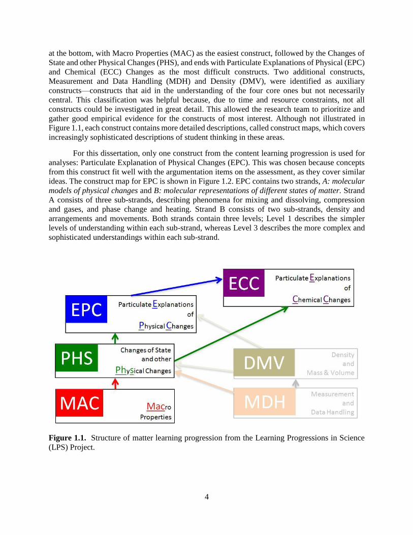
4

at the bottom, with Macro Properties (MAC) as the easiest construct, followed by the Changes of

State and other Physical Changes (PHS), and ends with Particulate Explanations of Physical (EPC)

and Chemical (ECC) Changes as the most difficult constructs. Two additional constructs,

Measurement and Data Handling (MDH) and Density (DMV), were identified as auxiliary

constructs—constructs that aid in the understanding of the four core ones but not necessarily

central. This classification was helpful because, due to time and resource constraints, not all

constructs could be investigated in great detail. This allowed the research team to prioritize and

gather good empirical evidence for the constructs of most interest. Although not illustrated in

Figure 1.1, each construct contains more detailed descriptions, called construct maps, which covers

increasingly sophisticated descriptions of student thinking in these areas.

For this dissertation, only one construct from the content learning progression is used for

analyses: Particulate Explanation of Physical Changes (EPC). This was chosen because concepts

from this construct fit well with the argumentation items on the assessment, as they cover similar

ideas. The construct map for EPC is shown in Figure 1.2. EPC contains two strands, A: molecular

models of physical changes and B: molecular representations of different states of matter. Strand

A consists of three sub-strands, describing phenomena for mixing and dissolving, compression

and gases, and phase change and heating. Strand B consists of two sub-strands, density and

arrangements and movements. Both strands contain three levels; Level 1 describes the simpler

levels of understanding within each sub-strand, whereas Level 3 describes the more complex and

sophisticated understandings within each sub-strand.

Figure 1.1. Structure of matter learning progression from the Learning Progressions in Science

(LPS) Project.

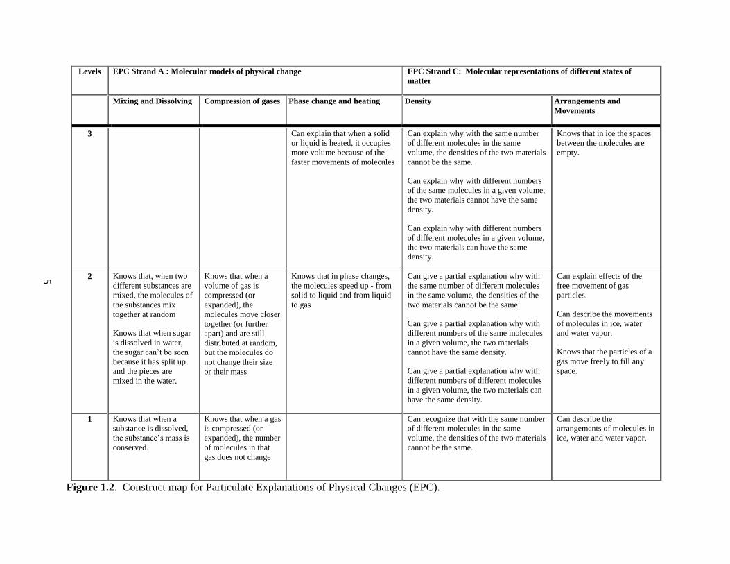
5

Levels EPC Strand A : Molecular models of physical change EPC Strand C: Molecular representations of different states of

matter

Mixing and Dissolving Compression of gases Phase change and heating Density Arrangements and

Movements

3 Can explain that when a solid

or liquid is heated, it occupies

more volume because of the

faster movements of molecules

Can explain why with the same number

of different molecules in the same

volume, the densities of the two materials

cannot be the same.

Can explain why with different numbers

of the same molecules in a given volume,

the two materials cannot have the same

density.

Can explain why with different numbers

of different molecules in a given volume,

the two materials can have the same

density.

Knows that in ice the spaces

between the molecules are

empty.

2 Knows that, when two

different substances are

mixed, the molecules of

the substances mix

together at random

Knows that when sugar

is dissolved in water,

the sugar can’t be seen

because it has split up

and the pieces are

mixed in the water.

Knows that when a

volume of gas is

compressed (or

expanded), the

molecules move closer

together (or further

apart) and are still

distributed at random,

but the molecules do

not change their size

or their mass

Knows that in phase changes,

the molecules speed up - from

solid to liquid and from liquid

to gas

Can give a partial explanation why with

the same number of different molecules

in the same volume, the densities of the

two materials cannot be the same.

Can give a partial explanation why with

different numbers of the same molecules

in a given volume, the two materials

cannot have the same density.

Can give a partial explanation why with

different numbers of different molecules

in a given volume, the two materials can

have the same density.

Can explain effects of the

free movement of gas

particles.

Can describe the movements

of molecules in ice, water

and water vapor.

Knows that the particles of a

gas move freely to fill any

space.

1 Knows that when a

substance is dissolved,

the substance’s mass is

conserved.

Knows that when a gas

is compressed (or

expanded), the number

of molecules in that

gas does not change

Can recognize that with the same number

of different molecules in the same

volume, the densities of the two materials

cannot be the same.

Can describe the

arrangements of molecules in

ice, water and water vapor.

Figure 1.2. Construct map for Particulate Explanations of Physical Changes (EPC).

6

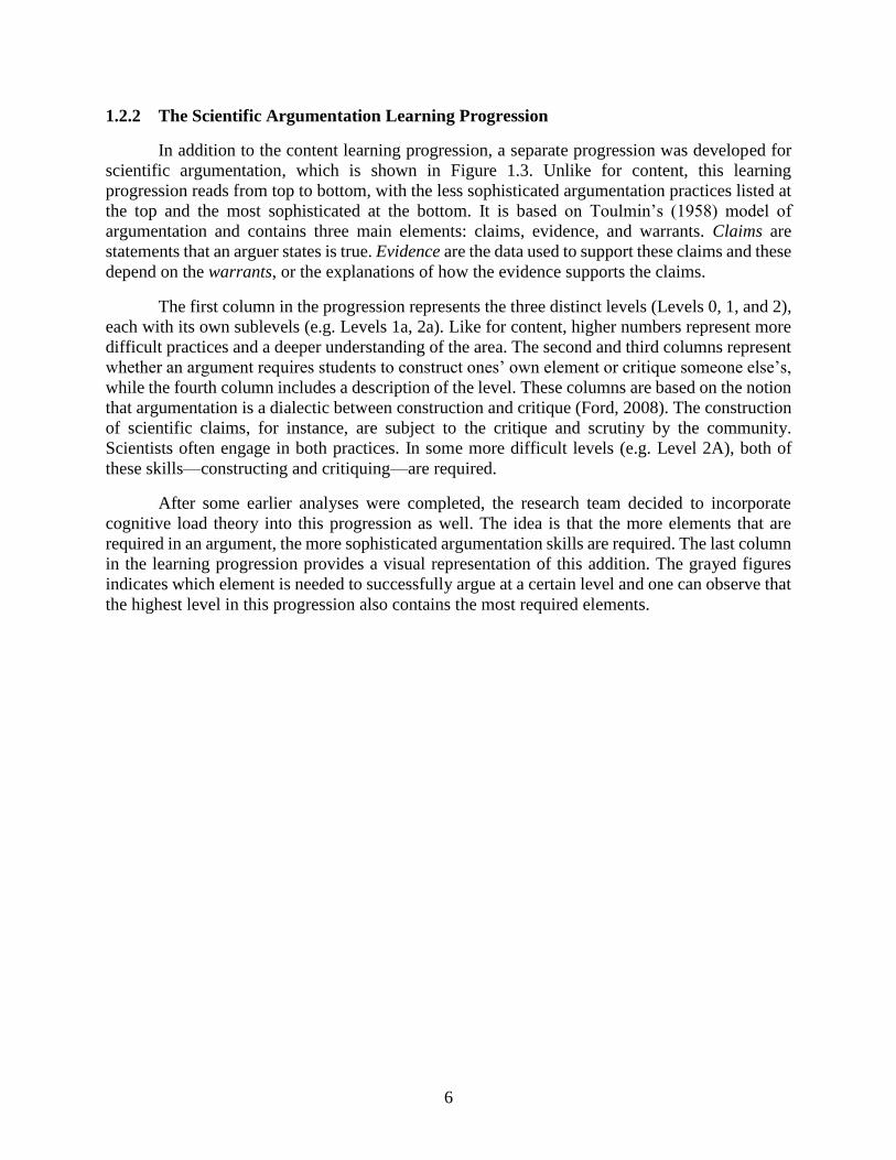
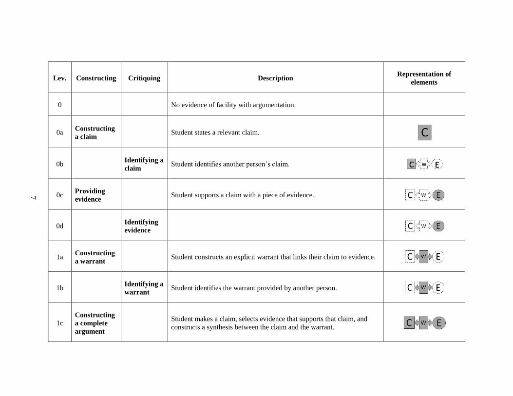
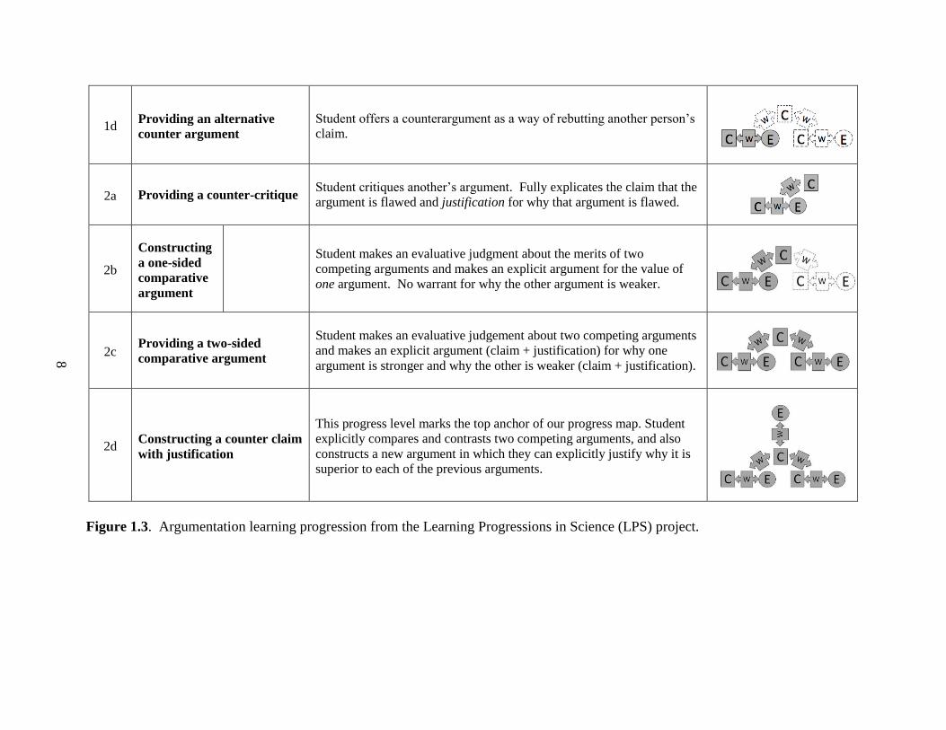
1.2.2 The Scientific Argumentation Learning Progression

In addition to the content learning progression, a separate progression was developed for

scientific argumentation, which is shown in Figure 1.3. Unlike for content, this learning

progression reads from top to bottom, with the less sophisticated argumentation practices listed at

the top and the most sophisticated at the bottom. It is based on Toulmin’s (1958) model of

argumentation and contains three main elements: claims, evidence, and warrants. Claims are

statements that an arguer states is true. Evidence are the data used to support these claims and these

depend on the warrants, or the explanations of how the evidence supports the claims.

The first column in the progression represents the three distinct levels (Levels 0, 1, and 2),

each with its own sublevels (e.g. Levels 1a, 2a). Like for content, higher numbers represent more

difficult practices and a deeper understanding of the area. The second and third columns represent

whether an argument requires students to construct ones’ own element or critique someone else’s,

while the fourth column includes a description of the level. These columns are based on the notion

that argumentation is a dialectic between construction and critique (Ford, 2008). The construction

of scientific claims, for instance, are subject to the critique and scrutiny by the community.

Scientists often engage in both practices. In some more difficult levels (e.g. Level 2A), both of

these skills—constructing and critiquing—are required.

After some earlier analyses were completed, the research team decided to incorporate

cognitive load theory into this progression as well. The idea is that the more elements that are

required in an argument, the more sophisticated argumentation skills are required. The last column

in the learning progression provides a visual representation of this addition. The grayed figures

indicates which element is needed to successfully argue at a certain level and one can observe that

the highest level in this progression also contains the most required elements.

7

Lev. Constructing Critiquing Description Representation of

elements

0 No evidence of facility with argumentation.

0a Constructing

a claim Student states a relevant claim.

0b Identifying a

claim Student identifies another person’s claim.

0c Providing

evidence Student supports a claim with a piece of evidence.

0d Identifying

evidence

1a Constructing

a warrant Student constructs an explicit warrant that links their claim to evidence.

1b Identifying a

warrant Student identifies the warrant provided by another person.

1c Constructing

a complete

argument

Student makes a claim, selects evidence that supports that claim, and

constructs a synthesis between the claim and the warrant.

8

1d Providing an alternative

counter argument

Student offers a counterargument as a way of rebutting another person’s

claim.

2a Providing a counter-critique

Student critiques another’s argument. Fully explicates the claim that the

argument is flawed and justification for why that argument is flawed.

2b

Constructing

a one-sided

comparative

argument

Student makes an evaluative judgment about the merits of two

competing arguments and makes an explicit argument for the value of

one argument. No warrant for why the other argument is weaker.

2c Providing a two-sided

comparative argument

Student makes an evaluative judgement about two competing arguments

and makes an explicit argument (claim + justification) for why one

argument is stronger and why the other is weaker (claim + justification).

2d Constructing a counter claim

with justification

This progress level marks the top anchor of our progress map. Student

explicitly compares and contrasts two competing arguments, and also

constructs a new argument in which they can explicitly justify why it is

superior to each of the previous arguments.

Figure 1.3. Argumentation learning progression from the Learning Progressions in Science (LPS) project.

9

1.2.3 Complex Tasks for 2013-2014 Data Collection

LPS data from the 2013-2014 school year is used for this dissertation. In response to the

NGSS, the items for this data collection were organized into “complex tasks”, which consist of (1)

argumentation items assessing argumentation competency in a specific scientific context (e.g. two

students arguing over what happens to gas particles placed in a container, (2) content science items

situated within the same scientific context (e.g. what happens when you insert gas particles into a

sealed container), and (3) content science items assessing knowledge of other concepts in the same

science domain but not so closely associated with the context (e.g. compare the movement of liquid

water molecules with the movement of ice molecules). In this dissertation, these three item types

will be referred to as “argumentation”, “embedded content”, and “content” items, respectively.

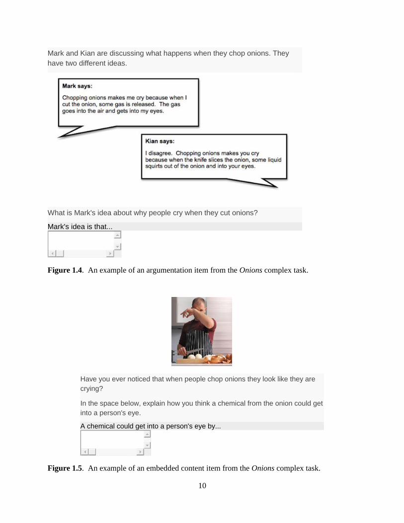
Figures 1.4, 1.5, and 1.6 illustrate, respectively, an example of each type of item from the same

complex task (i.e. onions).

Note that the embedded content and the argumentation items share common stimulus

materials because they occur within the same context (e.g. why do people cry when they cut

onions?). Content items do not share any of the stimulus materials and resemble more traditional

content items. They are general questions with no specific context. They are, however, presented

along with the other two item types.

In total, there are three complex tasks that cover different contexts including chopping

onions, placing gas particles in a jar, and dissolving sugar in water. In this dissertation, they will

be referred to as “onions”, “gases”, and “sugar”, respectively. The assumption behind this

“complex task” organization is tying in both the domain knowledge of the structure of matter in

addition to the practice of scientific argumentation. Instead of just testing decontextualized content

matter (content items), contextualized content items (embedded content) and contextualized

argumentation items (argumentation) are presented alongside one another. By presenting these

three types of items on the same assessment, the relationship among content domain knowledge

and scientific argumentation competency can be further explored.

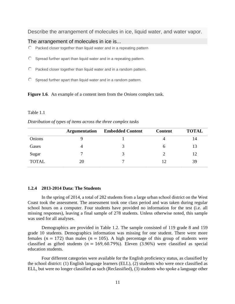
For the dissertation, a subset of the original 2013-2014 LPS data is used, for a final total of

39 items across the three complex tasks. Table 1.1 illustrates the distribution of these final item

types across the three different contexts. There were 20 argumentation items, 7 embedded content,

and 12 content items. All embedded content and content items were scored following the EPC

construct map (shown in Figure 1.2), while all argumentation items were scored following the

argumentation learning progression (shown in Figure 1.3).

10

Figure 1.4. An example of an argumentation item from the Onions complex task.

Figure 1.5. An example of an embedded content item from the Onions complex task.

Mark and Kian are discussing what happens when they chop onions. They

have two different ideas.

What is Mark's idea about why people cry when they cut onions?

Mark's idea is that...

Have you ever noticed that when people chop onions they look like they are

crying?

In the space below, explain how you think a chemical from the onion could get

into a person's eye.

A chemical could get into a person's eye by...

11

Figure 1.6. An example of a content item from the Onions complex task.

Table 1.1

Distribution of types of items across the three complex tasks

Argumentation Embedded Content Content TOTAL

Onions 9 1 4 14

Gases 4 3 6 13

Sugar 7 3 2 12

TOTAL 20 7 12 39

1.2.4 2013-2014 Data: The Students

In the spring of 2014, a total of 282 students from a large urban school district on the West

Coast took the assessment. The assessment took one class period and was taken during regular

school hours on a computer. Four students have provided no information for the test (i.e. all

missing responses), leaving a final sample of 278 students. Unless otherwise noted, this sample

was used for all analyses.

Demographics are provided in Table 1.2. The sample consisted of 119 grade 8 and 159

grade 10 students. Demographics information was missing for one student. There were more

females (𝑛 = 172) than males (𝑛 = 105). A high percentage of this group of students were

classified as gifted students (𝑛 = 169, 60.79%). Eleven (3.96%) were classified as special

education students.

Four different categories were available for the English proficiency status, as classified by

the school district: (1) English language learners (ELL), (2) students who were once classified as

ELL, but were no longer classified as such (Reclassified), (3) students who spoke a language other

Describe the arrangement of molecules in ice, liquid water, and water vapor.

The arrangement of molecules in ice is...

Packed closer together than liquid water and in a repeating pattern

Spread further apart than liquid water and in a repeating pattern.

Packed closer together than liquid water and in a random pattern.

Spread further apart than liquid water and in a random pattern.

12

than English at home, but were never classified as an ELL (Fluent), and (4) students whose primary

language was English (English). The total counts for these four groups are 3, 110, 58, and 106,

respectively.

Table 1.2

Demographics for students who took the LPS assessment in Spring 2014 (N=278)

Frequency* Percentage*

Grade

Eighth 119 42.81

Tenth 159 57.19

TOTAL 278 100.00

Sex

Female 172 61.87

Male 105 37.77

TOTAL 277 99.64

English Proficiency Classification

English language learner (ELL) 3 1.06

Reclassified 110 39.57

Fluent 58 20.86

English 106 38.13

TOTAL 277 99.64

Classification: Gifted

Yes 169 60.79

No 108 38.85

TOTAL 277 99.64

Classification: Special Education

Yes 11 3.96

No 266 95.68

TOTAL 277 99.64

*Note: Due to missing data, not all frequencies equal 278 nor do all percentages equal 100.

13

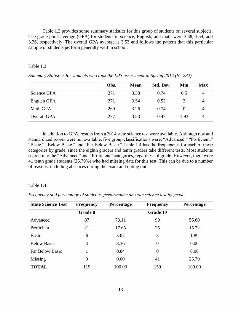
Table 1.3 provides some summary statistics for this group of students on several subjects.

The grade point average (GPA) for students in science, English, and math were 3.38, 3.54, and

3.26, respectively. The overall GPA average is 3.53 and follows the pattern that this particular

sample of students perform generally well in school.

Table 1.3

Summary Statistics for students who took the LPS assessment in Spring 2014 (N=282)

Obs. Mean Std. Dev. Min Max

Science GPA 271 3.38 0.74 0.5 4

English GPA 271 3.54 0.52 2 4

Math GPA 269 3.26 0.74 0 4

Overall GPA 277 3.53 0.42 1.93 4

In addition to GPA, results from a 2014 state science test were available. Although raw and

standardized scores were not available, five group classifications were: “Advanced,” “Proficient,”

“Basic,” “Below Basic,” and “Far Below Basic.” Table 1.4 has the frequencies for each of these

categories by grade, since the eighth graders and tenth graders take different tests. Most students

scored into the “Advanced” and “Proficient” categories, regardless of grade. However, there were

41 tenth grade students (25.79%) who had missing data for this test. This can be due to a number

of reasons, including absences during the exam and opting out.

Table 1.4

Frequency and percentage of students’ performance on state science test by grade

State Science Test Frequency Percentage Frequency Percentage

Grade 8 Grade 10

Advanced 87 73.11 90 56.60

Proficient 21 17.65 25 15.72

Basic 6 5.04 3 1.89

Below Basic 4 3.36 0 0.00

Far Below Basic 1 0.84 0 0.00

Missing 0 0.00 41 25.79

TOTAL 119 100.00 159 100.00

14

1.3 The Three Research Areas

The purpose of this dissertation is to investigate sources of validity evidence to determine:

(1) whether student responses to these complex tasks reflect student understanding in the structure

of matter content domain and their scientific argumentation competency, and (2) to explore the

relationship between these two learning progressions. I plan to accomplish these two interrelated

goals by applying various explanatory item response models (EIRM; De Boeck & Wilson, 2004).

These models can be useful when gathering validity evidence for assessments as they can help

explain student learning and group differences.

As all aspects of validity evidence are important to consider when evaluating assessments,

these sources of evidence will be explored throughout this dissertation, with the main focus on

evidence related to test content, internal structure, and relation to other variables. Evidence related

to response processes and consequential validity are of lower interest as the first was already

explored during the test development process (which followed the BEAR Assessment System or

BAS; Wilson & Sloane, 2000) and the latter because the test is a low-stakes test, administered only

once, for research purposes only and had no effects on students’ grades.

The next chapter explores the dimensionality of the test by comparing unidimensional,

between-item multidimensional, and Rasch testlet models to find the best-fitting model for the

data. The second research area focuses on person and person-by-item predictors through applying

a latent regression model and a differential item functioning (DIF) model, respectively. The last

research area uses a linear logistic test model (LLTM) to identify vital item features for the test.

Throughout all papers, validity evidence for test content, internal structure, and relation to other

variables will be discussed.

1.3.1 Model Selection and Software

This research is interested in comparing a group of models to find the relative best-fitting

one that can explain the data well while also having a reasonable number of parameters. When

models are nested, a likelihood ratio test can be used for direct comparison. However, when models

are not nested but use the same data, two common measures can be used for model selection:

Akaike’s Information Criteria (AIC; Akaike, 1974) and the Bayesian Information Criterion (BIC;

Schwarz, 1978). For both criteria, the model with the lowest value is preferred as it indicates a

better fit.

AIC is defined as:

AIC = 𝐺2 + 2𝑝 + 𝑇 (1.1)

where 𝐺2 is the model deviance, 𝑝 is the number of parameters, and 𝑇 is an arbitrary constant.

Since a lower value is preferred, one can see that a model is penalized for having more parameters,

as denoted by the 2𝑝.

15

Similar to AIC, BIC is defined as:

BIC = 𝐺2 + 𝑝 log (𝑛) (1.2)

where 𝐺2 and 𝑝 is the same as in Equation 1.1 and 𝑛 is the sample size. Like the AIC, the BIC also

includes a penalty for a larger number of parameters. However, the BIC also includes the prior

distribution, as denoted by the inclusion of the sample size.

Cleaning the data, descriptive analyses, and some graphs were completed using Stata 11

(StataCorp, 2009). Wright maps were generated using the WrightMap package (Torres Irribarra

& Freund, 2016) in R (R Core Team, 2015). Unless otherwise noted, ConQuest 3.0 (Adams, Wu,

& Wilson, 2012) was used for all Rasch analyses in this paper. Estimation methods, constraints,

and other settings may differ for each chapter and will be described accordingly.

16

Chapter 2: Multidimensional modeling of the complex tasks

2.1 Introduction

The complex tasks in the LPS assessment, described in the first chapter, consist of three

item types (content, embedded content, and argumentation) that were designed to follow some of

the recommendations from the Next Generation Science Standards (NGSS; NGSS Lead States,

2013). This chapter investigates the relationship of these item types by applying multidimensional

item response models, with the goal that this analysis will shed insight into the relationship

between the scientific practice of argumentation and the content domain of structure of matter.

Multidimensional models can provide more complex descriptions regarding student learning than

unidimensional models (Briggs & Wilson, 2003; Hartig & Höhler, 2009), such as modeling

nuisance dimensions (Wang & Wilson, 2005), group differences (Liu, Wilson, & Paek, 2008;

Walker and Beretvas, 2003; Walker, Zhang, & Surber, 2008) and latent covariance structures (Wu

& Adams, 2006). Thus, as an initial step towards understanding the nature of these complex tasks,

a dimensionality analysis is appropriate to investigate the relationships between these three item

types. Specifically, the main research questions for this chapter are:

RQ1. What is the relationship between scientific argumentation items, content knowledge

items, and the embedded content items in the complex tasks? More specifically,

what can these three item types reveal about the relationship between scientific

content and scientific argumentation?

To explore this research question, several models—of varying dimensions—are analyzed

and compared to find the best-fitting model. This includes a model assuming (1) the items measure

one latent dimension (e.g. an overall science proficiency dimension), (2) the items measure

multiple latent dimensions (e.g. separate argumentation and content knowledge dimensions), and

(3) the presence of a nuisance dimension (e.g. context of items is not of interest, but is important

to take into account). These models are described in detail in the next section. By applying

multidimensional item response models, multiple relationships can be investigated, such as the

relationship between the embedded content and the content items, and in turn, allow for a more

substantive look into the three item types.

17

2.2 Unidimensional, Between-item Multidimensional, and Testlet Models

To investigate the dimensionality of these item types, several models are compared to find

the relative best-fitting model. First, a unidimensional partial credit model (PCM; Masters, 1982)

is applied to the data to test the assumption that the items measure only one underlying latent

construct. This model serves as a baseline to test whether the complexity of multidimensional

models are actually needed for this assessment. The PCM was chosen because it can handle all the

items in the assessment, which include dichotomously and polytomously scored items. It models

the log odds of the probability that student 𝑝 with ability 𝜃𝑝 will respond in category 𝑗 instead of

category 𝑗 − 1 on item 𝑖, as shown in Equation 2.1 below:

log(𝑃(𝑋𝑖=𝑗|𝜃𝑝)

𝑃(𝑋𝑖=𝑗−1|𝜃𝑝)) = 𝜃𝑝 − 𝛿𝑖𝑗 (2.1)

where 𝛿𝑖𝑗 is a parameter for the difficulty for step 𝑗 of item 𝑖 and 𝜃𝑝~𝑁(0, 𝜎𝜃𝑝

2 ).

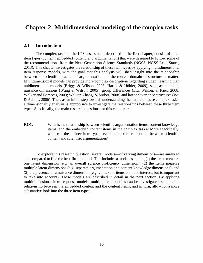
A graphical representation of this model is shown in Figure 2.1. To read this graphic, recall

that there are three item types (content, argumentation, and embedded content) and three item

contexts (sugar, onions, and gases), resulting in nine ‘context by type’ item combinations. These

item combinations are shown as boxes throughout Figures 2.1 to 2.6. As an example, “SA” denotes

an argumentation item that is about sugar dissolving in water, whereas “GE” is an embedded

content item about gases. For Figure 2.1, notice that all nine combinations of items, regardless of

context or type, are presumed to measure the same underlying latent dimension in this model which

is represented by the circle. This underlying dimension is called “science” here, since all items are

intended to measure science1.

1 Note that naming this dimension “science” is simply to show its generalness compared to the other models described

later. The domain of science is large and these items as a whole would only measure a tiny portion of this domain. To

be even more specific, this dimension could be titled “scientific argumentation and particulate explanations of physical

changes.” For simplification, the simpler, less verbose title seems apt here.

18

Figure 2.1. Diagram for the unidimensional model.

This unidimensional model is not necessarily of interest as the test was designed to measure

two latent constructs—scientific argumentation and structure of matter content. Thus, a two-

dimensional model would ideally fit this data better than the unidimensional model. For validity

purposes, it is important to test the assumption that a multidimensional model would fit the data

statistically significantly better than the unidimensional version.

One way to model a multidimensional extension to the PCM includes adding a dimensional

subscript 𝑑 to the person proficiency 𝜃𝑝. Thus, instead of a scalar, the person proficiency is now

written as a vector 𝜽𝑝𝑑 = (𝜃11, … , 𝜃1𝐷 , … , 𝜃𝑝𝐷) which contains the latent trait estimates for each

person 𝑝 on each dimension 𝑑. For example, in a two-dimensional model, each person would have

two ability estimates, one for each of the dimensions. For a three-dimensional model, each person

would have three ability estimates and so on. The between-item multidimensional extension is

illustrated in Equation 2.2, where it is assumed that each item measures just one dimension (i.e.,

between-item dimensionality; Wang, Wilson, & Adams, 1997). This model fits well with the LPS

data, as the items in this assessment have one underlying dimension that it measures (i.e.

argumentation or content, but not both).

log(𝑃(𝑋𝑖=𝑗|𝜃𝑝𝑑)

𝑃(𝑋𝑖=𝑗−1|𝜃𝑝𝑑)) = 𝜃𝑝𝑑 − 𝛿𝑖𝑗 (2.2)

The 𝛿𝑖𝑗 has the same meaning as in Equation 2.1. All item step parameters, then, would continue

to have only one estimate.

19

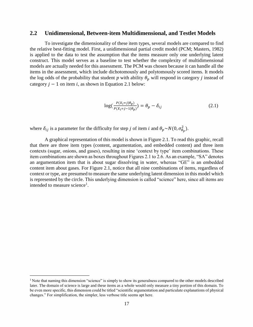
Figure 2.2 shows the two-dimensional between-item model. While Figure 2.1 had one

circle representing a latent dimension, Figure 2.2 has two circles: one representing content and the

other representing argumentation. The curved arrow connecting these two dimensions suggests

that these dimensions are correlated. In this model, the items are assumed to measure one of two

possible dimensions: scientific argumentation or structure of matter content. The embedded

content items are assumed to measure the content dimension because they are content items that

are embedded to a specific everyday context. In addition, these items were scored following the

content construct map. If this model is statistically more significant than the model shown in Figure

2.1, then it suggests that the items measure two distinct, correlated dimensions, rather than just one

latent dimension.

Figure 2.2. Diagram for the two-dimensional between-item model.

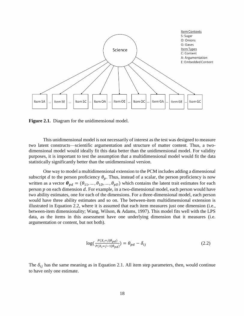
While the items were designed with two underlying constructs in mind, it is still useful to

test whether this was actually true. Comparing the two-dimensional model with a unidimensional

model is appropriate, as is adding an additional dimension. Thus, a three-dimensional between-

item model, where each of the three types of items were assumed to measure three distinct, but

correlated dimensions, is tested. This model, shown in Figure 2.3, is similar to the previous model,

but the embedded content items are considered to measure its own unique dimension. That is, the

embedded content items measure a distinct construct that differs from the content items. If this

model provides a statistically significantly better fit than the previous model (represented by Figure

2.2) and there is a meaningful difference between the models’ effect size, then this suggests that

the embedded content items are measuring something other than simply the same science content.

20

Figure 2.3. Diagram for a three-dimensional between-item model.

While the two- and three-dimensional between-item models take into account the differing

item types, they do not account for the similar contexts (e.g. sugar, onions, gases) of some of the

items. Although there is no particular interest in these contexts, they may still be important to

account for due to the possible violation of local independence. Two of the three item types in the

complex tasks (argumentation and embedded content) share a common context that may result in

local dependence. In addition, all items within a complex task unit were grouped together due to

similar content coverage. While the content items do not share the same stimuli as some of the

argumentation and embedded content items, they cover similar content ideas as the other items

within the same task. Checking the local independence assumption for these complex tasks seem

appropriate for this data.

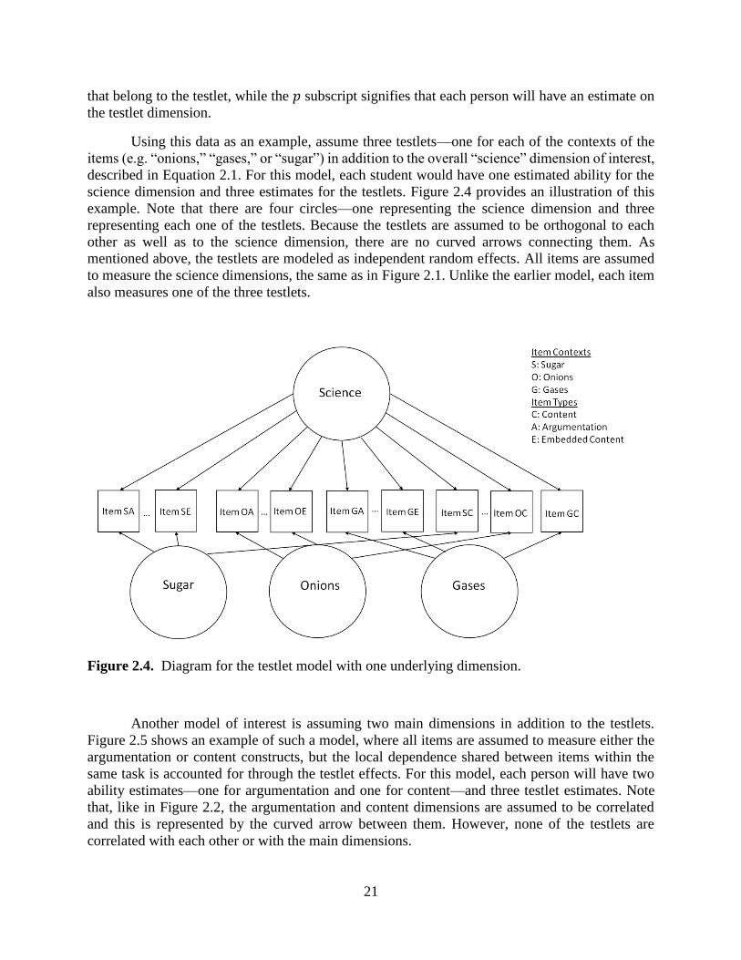
The Rasch testlet model (Wang & Wilson, 2005) is a multidimensional model that can

account for this local dependence between items, especially when this dependency is not of interest

(e.g. a “nuisance” dimension). This model is written as:

log (𝑃(𝑋𝑖=𝑗|𝜃𝑝𝑑)

𝑃(𝑋𝑖=𝑗−1|𝜃𝑝𝑑)) = 𝜃𝑝𝑑 − 𝛿𝑖𝑗 + 𝛾𝑝𝑑(𝑖) (2.3)

where, like in the earlier equations, the log odds of the probabilities that person 𝑝 scoring in

category 𝑗 as opposed to category 𝑗 − 1 to item 𝑖 is modeled. The parameters 𝛿𝑖𝑗 and 𝜃𝑝𝑑 have the

same meaning as in Equation 2.2. Note that this means all items will continue to have the same

number of difficulty parameters, 𝛿𝑖𝑗, as they remain fixed effects. The 𝛾𝑝𝑑(𝑖) is the random effect

of testlet 𝑑(𝑖) with 𝛾𝑝𝑑(𝑖)~ 𝑁(0, 𝜎𝛾𝑝𝑑(𝑖)2 ). Each testlet is modeled as an independent random effect

that is orthogonal to each other and to any other dimensions. The 𝑖 subscript signifies the items

21

that belong to the testlet, while the 𝑝 subscript signifies that each person will have an estimate on

the testlet dimension.

Using this data as an example, assume three testlets—one for each of the contexts of the

items (e.g. “onions,” “gases,” or “sugar”) in addition to the overall “science” dimension of interest,

described in Equation 2.1. For this model, each student would have one estimated ability for the

science dimension and three estimates for the testlets. Figure 2.4 provides an illustration of this

example. Note that there are four circles—one representing the science dimension and three

representing each one of the testlets. Because the testlets are assumed to be orthogonal to each

other as well as to the science dimension, there are no curved arrows connecting them. As

mentioned above, the testlets are modeled as independent random effects. All items are assumed

to measure the science dimensions, the same as in Figure 2.1. Unlike the earlier model, each item

also measures one of the three testlets.

Figure 2.4. Diagram for the testlet model with one underlying dimension.

Another model of interest is assuming two main dimensions in addition to the testlets.

Figure 2.5 shows an example of such a model, where all items are assumed to measure either the

argumentation or content constructs, but the local dependence shared between items within the

same task is accounted for through the testlet effects. For this model, each person will have two

ability estimates—one for argumentation and one for content—and three testlet estimates. Note

that, like in Figure 2.2, the argumentation and content dimensions are assumed to be correlated

and this is represented by the curved arrow between them. However, none of the testlets are

correlated with each other or with the main dimensions.

22

Figure 2.5. Diagram for the testlet model with two underlying dimensions.

For this chapter, the models shown in Figure 2.4 and Figure 2.5 will be referred to as the

“one-dimensional testlet model” and the “two-dimensional testlet model,” respectively. The testlet

models are considered to be within-item multidimensional models (Wang, Wilson, & Adams,

1997), as all items map onto the main science, argumentation or content dimension and onto one

of the three testlets.

ConQuest 3.0 (Adams, Wu, & Wilson, 2012) was used with the default settings, which

used Gauss-Hermite Quadrature estimation. Monte Carlo estimation was used for the testlet

models, due to the large number of dimensions. For instance, in the two-dimensional testlet

models, five dimensions are estimated (two main dimensions and three testlet dimensions). A total

of five models will be compared in this chapter: the unidimensional model, two multidimensional

between-item models, and two testlet models. For model identification, the person mean for each

analysis was constrained to 0.00 on all dimensions.

23

2.3 Results

The results are divided into three sections. First, the results for the between-item

multidimensional models are presented, followed by the results for the testlet models. Finally, all

five models are compared to each other using the model selection criteria, described in Chapter 1,

to see which has the best statistical fit.

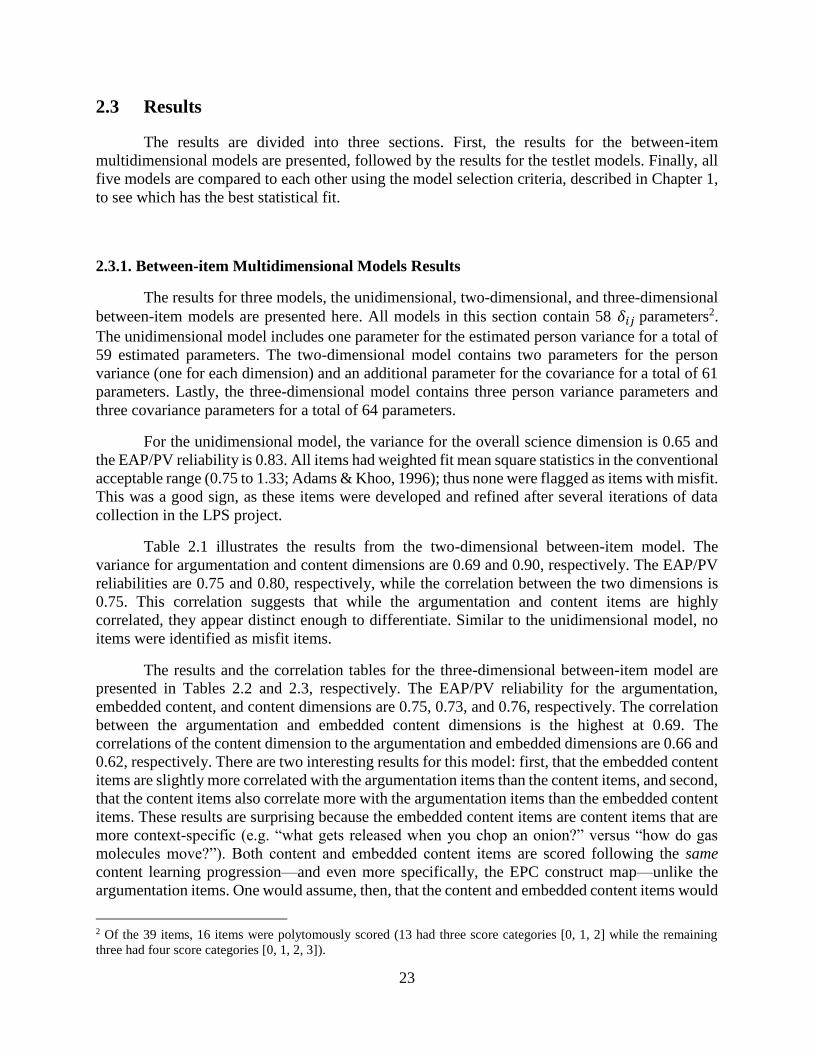
2.3.1. Between-item Multidimensional Models Results

The results for three models, the unidimensional, two-dimensional, and three-dimensional

between-item models are presented here. All models in this section contain 58 𝛿𝑖𝑗 parameters2.

The unidimensional model includes one parameter for the estimated person variance for a total of

59 estimated parameters. The two-dimensional model contains two parameters for the person

variance (one for each dimension) and an additional parameter for the covariance for a total of 61

parameters. Lastly, the three-dimensional model contains three person variance parameters and

three covariance parameters for a total of 64 parameters.

For the unidimensional model, the variance for the overall science dimension is 0.65 and

the EAP/PV reliability is 0.83. All items had weighted fit mean square statistics in the conventional

acceptable range (0.75 to 1.33; Adams & Khoo, 1996); thus none were flagged as items with misfit.

This was a good sign, as these items were developed and refined after several iterations of data

collection in the LPS project.

Table 2.1 illustrates the results from the two-dimensional between-item model. The

variance for argumentation and content dimensions are 0.69 and 0.90, respectively. The EAP/PV

reliabilities are 0.75 and 0.80, respectively, while the correlation between the two dimensions is

0.75. This correlation suggests that while the argumentation and content items are highly

correlated, they appear distinct enough to differentiate. Similar to the unidimensional model, no

items were identified as misfit items.

The results and the correlation tables for the three-dimensional between-item model are

presented in Tables 2.2 and 2.3, respectively. The EAP/PV reliability for the argumentation,

embedded content, and content dimensions are 0.75, 0.73, and 0.76, respectively. The correlation

between the argumentation and embedded content dimensions is the highest at 0.69. The

correlations of the content dimension to the argumentation and embedded dimensions are 0.66 and

0.62, respectively. There are two interesting results for this model: first, that the embedded content

items are slightly more correlated with the argumentation items than the content items, and second,

that the content items also correlate more with the argumentation items than the embedded content

items. These results are surprising because the embedded content items are content items that are

more context-specific (e.g. “what gets released when you chop an onion?” versus “how do gas

molecules move?”). Both content and embedded content items are scored following the same

content learning progression—and even more specifically, the EPC construct map—unlike the

argumentation items. One would assume, then, that the content and embedded content items would

2 Of the 39 items, 16 items were polytomously scored (13 had three score categories [0, 1, 2] while the remaining

three had four score categories [0, 1, 2, 3]).

24

be more correlated with each other than with items scored with a completely different learning

progression (i.e. argumentation). However, based on these results, it seems that the context of the

item plays a significant role for the correlation between the argumentation and the embedded

content items. It is unclear why the correlation for the content items and argumentation are higher

than for the embedded content items. This may simply be due to the few embedded content items.

Like the earlier two models, no items were identified as misfit items.

Table 2.1

Results for the two-dimensional between-item model

Argumentation Content

Variance 0.69 0.90

EAP/PV Reliability 0.75 0.80

Correlation 0.75

Table 2.2

Results for three-dimensional between-item model

Argumentation Embedded Content

Variance 0.69 1.04 1.69

EAP/Reliability 0.75 0.73 0.76

Table 2.3

Correlation table for the three-dimensional between-item model

Argumentation Content

Embedded 0.69 0.62

Content 0.66 --

Because the unidimensional, two-dimensional, and three-dimensional between-item

models are nested, likelihood ratio tests can be used to directly investigate which models fit

statistically significantly better. For these tests, the p-value was adjusted because it is at the

boundary of the parameter space (Rabe-Hesketh & Skrondal, 2008, pp. 69). Results from the

likelihood ratio test suggests that the two-dimensional between-item model has a better fit than the

unidimensional model (𝜒2 = 66.59, 𝑑𝑓 = 2, 𝑝 < 0.001).

25

A likelihood ratio test was also used to compare the fit of the two-dimensional and three-

dimensional between-item models. The three-dimensional model had a statistically significantly

better fit than the two-dimensional model (𝜒2 = 89.09, 𝑑𝑓 = 3, 𝑝 < 0.001), suggesting that the

three-dimensional model is more appropriate for the LPS data. Because this model had the superior

fit of the three described in this section, it will be explored in further detail.

First, delta dimensional alignment (DDA; Schwartz & Ayers, 2011)—a technique for

transforming multidimensional analyses to place dimensions on a common metric—was applied

so that the three dimensions can be directly compared. This adjustment was needed as the results

from multidimensional models cannot be directly compared because the mean of the student ability

distributions for each dimension were constrained to 0.00 so that the model could be identified3.

Because of this constraint, it is unreasonable to assume that the students have the same distribution

on all dimensions, making comparisons across dimensions not meaningful.

DDA adjusts the item parameters so that these comparisons can be made. Recall that the

item step parameters in Equations 2.1 to 2.4 are denoted as 𝛿𝑖𝑗. This can also be rewritten as 𝛿𝑖 +

𝜏𝑖𝑗, where 𝛿𝑖 is the mean of the step difficulties, or the overall item difficulty, and 𝜏𝑖𝑗 is the

deviance from this overall mean for step 𝑗 of item 𝑖. Thus, the transformation for the item

parameters are:

𝛿𝑖𝑑(𝑡𝑟𝑎𝑛𝑠𝑓𝑜𝑟𝑚𝑒𝑑) = 𝛿𝑖𝑑(𝑚𝑢𝑙𝑡𝑖) (𝜎𝑑(𝑢𝑛𝑖)

𝜎𝑑(𝑚𝑢𝑙𝑡𝑖)) + 𝜇𝑑(𝑢𝑛𝑖) (2.4)

where 𝛿𝑖𝑑(𝑚𝑢𝑙𝑡𝑖) is the estimated item parameter from the multidimensional analysis, and 𝜎𝑑(𝑢𝑛𝑖)

and 𝜎𝑑(𝑚𝑢𝑙𝑡𝑖) are the standard deviations for the item difficulty estimates in the unidimensional

and multidimensional models, respectively. 𝜇𝑑(𝑢𝑛𝑖) is the mean of the item difficulty estimates

from the unidimensional model.

To transform the step parameters, the adjustment is:

𝜏𝑖𝑗𝑑(𝑡𝑟𝑎𝑛𝑠𝑓𝑜𝑟𝑚𝑒𝑑) = 𝜏𝑖𝑗𝑑(𝑚𝑢𝑙𝑡𝑖)(𝜎𝑑(𝑢𝑛𝑖)

𝜎𝑑(𝑚𝑢𝑙𝑡𝑖)) (2.5)

where 𝜏𝑖𝑗𝑑(𝑚𝑢𝑙𝑡𝑖)is the step parameter obtained from the multidimensional analysis and 𝜎𝑑(𝑢𝑛𝑖) and

𝜎𝑑(𝑚𝑢𝑙𝑡𝑖) are the same as in Equation 2.4. After transforming these item and step parameters to the

3 As an alternative to constraining the student ability distributions to 0.00 for model identification, the sum of the item

difficulties can also be constrained to 0.00 by setting the last item to the negative sum of all other items on the

assessment.

26

same logit metric, the student abilities for each dimension can be re-estimated using these

transformed parameters as anchors. Then, direct comparisons across dimensions can be made.

Table 2.4 illustrates the updated results, including estimated population means, variances,

and reliabilities. The estimated population mean for the argumentation, embedded content, and

content dimensions are -1.48, -0.86, and -1.16 logits, respectively. While the argumentation

dimension has the lowest estimated mean, it also has the lowest variance, suggesting that the

students performed more similarly than in the other dimensions. The content dimension, on the

other hand, had a slightly higher estimated mean, but had a much larger variance. This difference

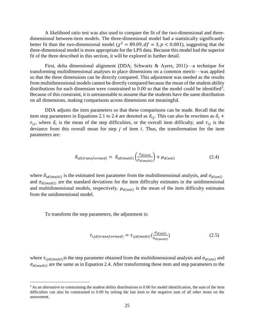
is clearly shown in the Wright map, shown in Figure 2.6.

Table 2.4

Results for three-dimensional between-item model, after application of DDA

Argumentation Embedded Content

Person Mean (SE) -1.48 (0.06) -0.86 (0.07) -1.16 (0.09)

Variance 0.68 0.97 1.53

EAP/Reliability 0.75 0.73 0.75

The Wright map below has two distinct sections: one for the student ability distribution

and one for the item difficulty distribution. Both of these distributions use the same scale, the logit

scale, and this is found on the very right of the map. The Wright map is an extremely useful tool

for presenting these two different sorts of distributions meaningfully. When the student ability

estimate is the same as the item difficulty, then the student has a 50% chance of answering the

item correctly. If the student has a lower estimated ability than the item difficulty, then she has

less than a 50% chance of answering the item correctly. If the estimated ability is higher, then she

has more than a 50% chance of answering the item correctly.

The left three columns represent the student ability distributions—estimated from expected

a-posteriori values (EAP)—for the argumentation (ARG), embedded content (EMB), and content

(CON) dimensions, respectively. From the map, it is apparent that the distribution for the

argumentation dimension peaks at about -1.50 logits. The embedded content dimension has a

similar shape, but the peak is higher, suggesting that the embedded content items may be slightly

easier for the students. For the content dimension, the distribution is flatter and wider with no sharp

peak, which suggests that the content items on the assessment was less successful in discriminating

the students on this dimension.

The right-hand section of the Wright map lists the items difficulties. Using the same

notations as in Figures 2.1 to 2.5, the first letter refers to the context (e.g. “S” means it is an item

in the “sugar” context), while the second letter refers to the item type (e.g. “A” is an argumentation

item). In addition, the colors also denote the item type with blue, red, and green referring to

argumentation, embedded content, and content items, respectively. The darker shades symbolize

that the item was hypothesized to be easier, while the lighter shades suggest that the item was

27

hypothesized to be more difficult. For example, the dark blues represent Level 0 items, the medium

blue represent the Level 1 items, and the light blue represent the Level 2 items for argumentation.

Comparing the location of these items based on empirical data to the hypothesized difficulties

based on the learning progression is an important step for gathering validity evidence for internal

structure. If the hypothesized easier items cluster, or band, at the bottom of the Wright map, while

the hypothesized difficult items band at the top of the Wright map, then this provides good validity

evidence for the assessment.

28

Figure 2.6. Wright map for the three-dimensional between-item model, after delta dimensional alignment was applied. Blue, red, and

green represents argumentation, embedded content, and content items, respectively.

29

For the argumentation items, some banding is obvious. The four items on the lower left-

hand corner are distinctly the easiest items and there are five light blue items (near the center of

the Wright that are the most difficult. However, the other items in-between are less distinct with

some items easier than anticipated and others more difficult than anticipated. Most argumentation

items fell between the -4.00 and -2.00 logit range and were from all levels of the learning

progression.

Likewise for the embedded content and the content dimensions, the easiest and most

difficult items in these dimensions show some clear distinction. However, the items in the middle

do not band as intended. Most items lie between -4.00 and -2.00 logit. Overall, when comparing

the student distributions to the item distributions, the test was easy for many of the students, as

many items had an estimated difficulty of less than -2.00 logits, while there were many students

with higher estimated abilities. This suggests that either more difficult items are needed to explore

the dimensions further, or a more representative sample of students may be needed. Recall that

there are a large number of tenth graders and most students in this sample were classified as

“gifted” and performed generally well in school, as indicated by their overall GPA (see Chapter

1).

Lastly, one embedded content item is surprisingly the most difficult item on the assessment.

It is the only item to have an estimated threshold of more than 2.00 logit. Upon closer examination,

the item is in the sugar context and is an open-ended item, with four score categories. The point

on the Wright map reflects the third threshold of the item—meaning that very few students scored

a 3 on this item as compared to a 2, 1, or 0. In order to receive a score of 3 rather than 2 for this

item, students must mention both that the sugar molecules mixed with the water and that the sugar

stays the same substance (i.e. does not combine to form a new substance). Only 5 students have

scored a 3 (about 1.80%) compared to 99 who scored a 2 (about 35.61%). This indicates that this

item needs to be revisited to investigate whether students were given a fair opportunity to answer

at the highest score category (i.e. investigate how the item was worded).

Overall, while the three-dimensional between-item model is statistically more significant

than both the unidimensional and two-dimensional model, it is unclear exactly what the embedded

items are measuring. The results indicate that they are measuring something distinct from the

content dimension, even though these items are scored following a content construct map. They

are also more correlated with the argumentation items. This could be due to the shared stimuli of

the items sharing the same context and this local dependence will be explored further with the

testlet models.

2.3.2. Testlet Models Results

Two testlet models were investigated. For the one-dimensional testlet model, the estimated

variance for the science dimension is 0.60, while the EAP/PV reliability is 0.71. Both are slightly

lower than for the unidimensional model, but this is anticipated since presumably, the testlets

account for some of the variance. The variances for the “sugar,” “onions,” and “gases” testlets are

0.31, 0.28, and 0.36, respectively. The reliabilities are 0.35, 0.30, and 0.42, respectively. The low

reliabilities for the testlets are expected because of the small number of items per testlet. In

30

addition, they are uncorrelated to all other testlets or dimensions, so no additional information is

provided through any of the other items.

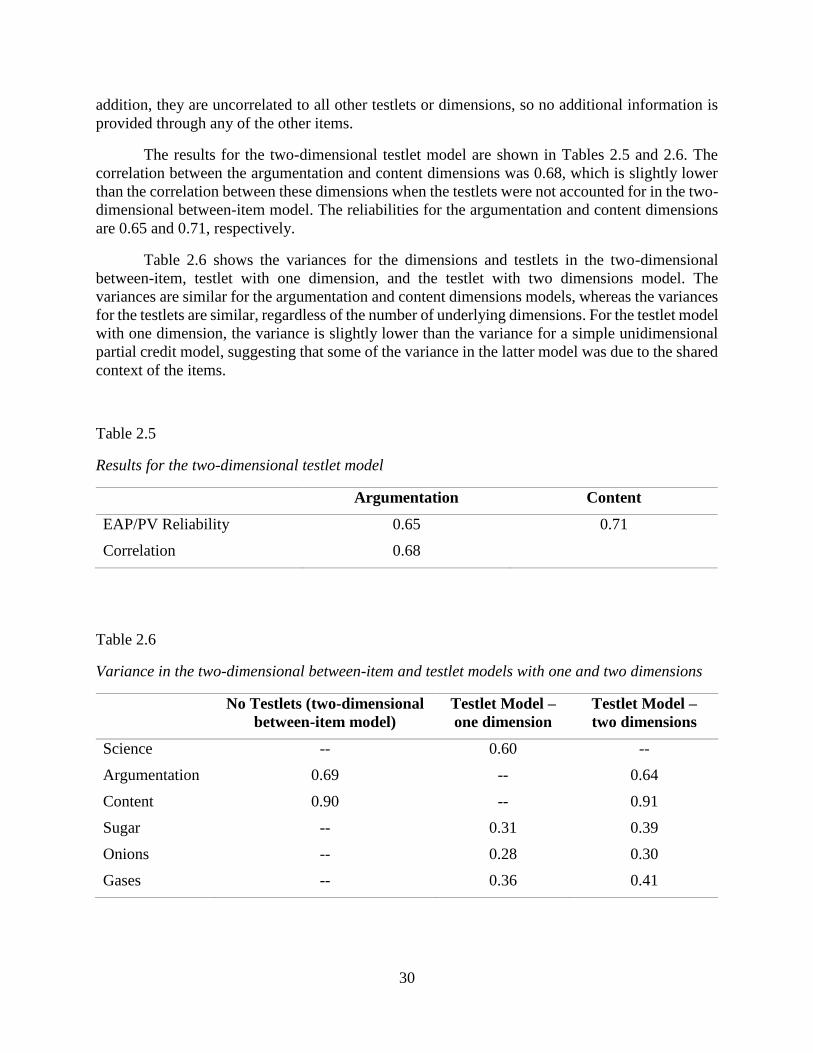
The results for the two-dimensional testlet model are shown in Tables 2.5 and 2.6. The

correlation between the argumentation and content dimensions was 0.68, which is slightly lower

than the correlation between these dimensions when the testlets were not accounted for in the two-

dimensional between-item model. The reliabilities for the argumentation and content dimensions

are 0.65 and 0.71, respectively.

Table 2.6 shows the variances for the dimensions and testlets in the two-dimensional

between-item, testlet with one dimension, and the testlet with two dimensions model. The

variances are similar for the argumentation and content dimensions models, whereas the variances

for the testlets are similar, regardless of the number of underlying dimensions. For the testlet model

with one dimension, the variance is slightly lower than the variance for a simple unidimensional

partial credit model, suggesting that some of the variance in the latter model was due to the shared

context of the items.

Table 2.5

Results for the two-dimensional testlet model

Argumentation Content

EAP/PV Reliability 0.65 0.71

Correlation 0.68

Table 2.6

Variance in the two-dimensional between-item and testlet models with one and two dimensions

No Testlets (two-dimensional

between-item model)

Testlet Model –

one dimension

Testlet Model –

two dimensions

Science -- 0.60 --

Argumentation 0.69 -- 0.64

Content 0.90 -- 0.91

Sugar -- 0.31 0.39

Onions -- 0.28 0.30

Gases -- 0.36 0.41

31

Like the between-item multidimensional models, the testlet models can also be compared

using a likelihood ratio test because they are nested models. When compared to the unidimensional

PCM model, the one-dimensional testlet model was statistically more significant (𝜒2 =146.27, 𝑑𝑓 = 23, 𝑝 < 0.001). When comparing the two testlet models, the two-dimensional

testlet model had a more statistically significant fit (𝜒2 = 75.25, 𝑑𝑓 = 2, 𝑝 < 0.001). This

matches the expectations of the LPS project, since the assessment was designed to measure two

distinct constructs (i.e. structure of matter content and argumentation). The better fit of the two-

dimensional over the one-dimensional testlet model provides empirical support for the assessment.

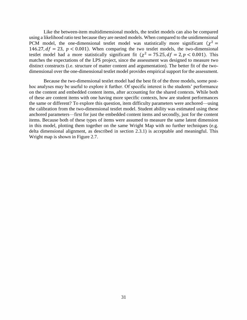
Because the two-dimensional testlet model had the best fit of the three models, some post-

hoc analyses may be useful to explore it further. Of specific interest is the students’ performance

on the content and embedded content items, after accounting for the shared contexts. While both

of these are content items with one having more specific contexts, how are student performances

the same or different? To explore this question, item difficulty parameters were anchored—using

the calibration from the two-dimensional testlet model. Student ability was estimated using these

anchored parameters—first for just the embedded content items and secondly, just for the content

items. Because both of these types of items were assumed to measure the same latent dimension

in this model, plotting them together on the same Wright Map with no further techniques (e.g.

delta dimensional alignment, as described in section 2.3.1) is acceptable and meaningful. This

Wright map is shown in Figure 2.7.

32

Figure 2.7. Wright map for two-dimensional testlet model. Only content and embedded content items are plotted.

33

Two student ability distributions are shown on the left-hand side of the Wright map: one

for embedded content and one for content. From the frequency distribution, more students appear

to have higher estimated abilities with the content items than for the embedded content items. The

mean for the embedded content and content items are -0.47 and 0.21 logit, respectively. For the

variance, it is 0.92 and 1.46, respectively. Thus, it seems that students performed slightly better on

the content items than the embedded content items.

The item difficulty distributions are on the right-hand side of the Wright map and uses the

same notations as Figures 2.1 to 2.5 and the earlier Wright map (i.e. first letter is for context,

second letter is for item type). For this map, only the embedded content and content items are

shown. The blue items represent items that measure the construct EPC strand A, while the red

items represent items that measure EPC strand B (discussed previously in Chapter 1). Like the

earlier Wright map, the darker shades represent the lower levels on the construct map (Level 1),

whereas the lighter shades represent higher levels (Levels 2 or 3).

As a whole, it appears that the range of item difficulties are similar for both embedded

content and content. Most item difficulties fell between -1.50 and 0.00 logit. In terms of banding,

a clear pattern does not emerge for either item type or construct strand. Items hypothesized as

easier (the darker shades) were not necessarily the easiest items while those hypothesized as the

most difficult (the lighter shades) did not have the highest difficulty.

There are a good number of students who have more than a 50% chance of answering all

the content items correctly. This is signified by the end of the student ability distribution for content

which goes past the most difficult content item. There are many fewer students on the upper end

of the embedded content distribution that have more than a 50% chance of answering all the

embedded content items correctly. In fact, the range of the embedded content items seem to fit the

distribution of the students well, despite only containing seven items.

While it is not immediately clear why the students struggled more with the embedded

content items than the content, there are a few possible explanations. First, students may be more

accustomed to the content items since they take on a familiar format. These items are general and

decontextualized, whereas the embedded content items provide specific contexts for application.

Students may simply have less experience with the application of structure of matter concepts to

actual real-life situations. Second, the embedded content items contain a greater number of open-

ended items (five of seven), while most of the content items are multiple-choice (ten of twelve).

Open-ended formats may be more difficult for students than multiple-choice items4.

2.3.3. Model Selection

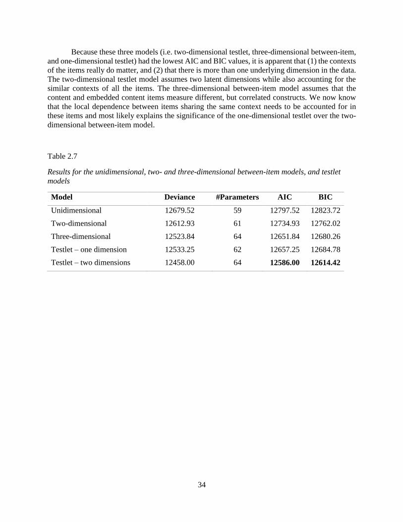
Finally, all five models can be compared using AIC and BIC values, the fit indices

described in Chapter 1. Table 2.7 illustrates the deviance, number of parameters, and AIC and BIC

for all the models. According to this table, the two-dimensional testlet model had the best fit since

it has the lowest AIC and BIC. The three-dimensional between-item model had the next best fit,

followed by the one-dimensional testlet model.

4 This hypothesis is explored in Chapter 4.

34

Because these three models (i.e. two-dimensional testlet, three-dimensional between-item,

and one-dimensional testlet) had the lowest AIC and BIC values, it is apparent that (1) the contexts

of the items really do matter, and (2) that there is more than one underlying dimension in the data.

The two-dimensional testlet model assumes two latent dimensions while also accounting for the

similar contexts of all the items. The three-dimensional between-item model assumes that the

content and embedded content items measure different, but correlated constructs. We now know

that the local dependence between items sharing the same context needs to be accounted for in

these items and most likely explains the significance of the one-dimensional testlet over the two-

dimensional between-item model.

Table 2.7

Results for the unidimensional, two- and three-dimensional between-item models, and testlet

models

Model Deviance #Parameters AIC BIC

Unidimensional 12679.52 59 12797.52 12823.72

Two-dimensional 12612.93 61 12734.93 12762.02

Three-dimensional 12523.84 64 12651.84 12680.26

Testlet – one dimension 12533.25 62 12657.25 12684.78

Testlet – two dimensions 12458.00 64 12586.00 12614.42

35

2.4 Discussion and Future Steps

In this chapter, several multidimensional models were applied to the LPS data in an attempt

to better understand the relationship between the three item types: content, argumentation, and

embedded content. A total of five models, one unidimensional, two between-item

multidimensional, and two testlet models, were compared. There were several interesting results

from the analyses. First, all the multidimensional models performed statistically significantly

better than the unidimensional model, which followed earlier results suggesting that argumentation

and content are distinct, but correlated dimensions. Second, the results also indicate that

accounting for the contexts of the items are important for this data, as the two-dimensional testlet

model has the best fit of the five models tested.

Another interesting result was the statistically significantly better fit of the three-

dimensional between-item model over the two-dimensional between-item model. This was

surprising because the embedded content and content items were scored using the same content

EPC construct map. Furthermore, the results showed that the embedded content items were more

correlated with the argumentation items than the content items, which also provides evidence of

the importance of accounting for the shared contexts of items. These results indicate that

accounting for the local dependence in each task is important.

The two-dimensional testlet model had the best fit of all five models tested. This reflects

the findings that (1) content and argumentation are separate dimensions, and (2) local dependence

needs to be taken into account. This is especially important when conceptualizing the content and

embedded content items. While both were scored using the same construct map, they cannot be

assumed to be equivalent. This was shown in the post-hoc analyses where student performances

on the two types of items differed. More students struggled with the embedded content than with

the content. While the cause of this difference is unclear, it seems safe to say that adding specific

contexts to content items may make them more difficult in general and they are no longer the same

as the decontextualized, general content items.

Some limitations for this data includes the limited number of items. While there appears to

be a good number of argumentation items, content and embedded content items were more limited.

In addition, the balance of open-ended to multiple-choice items for embedded content and content

were unequal. For a more detailed look into these two types of items, it may be more meaningful

to (1) have more items in general, and (2) have a good balance of multiple-choice and open-ended

formats.

In addition, as some of these models were mathematically complex (e.g. two-dimensional

testlet model has a total of five estimated dimensions), increasing the sample size would provide

more accurate estimations. Also, as mentioned previously, having a more representative sample as

well as a larger grade range of students may provide some additional information on the item types

and dimensions.

36

Chapter 3: Person regression models and person-by-item

models for explaining complex tasks

3.1 Introduction

Explanatory item response models (EIRMs) have the potential to provide explanations for

the item responses, rather than descriptive models where item responses are merely described by

the estimated parameters (De Boeck & Wilson, 2004). Latent regression is an example of an EIRM,

where the latent abilities are regressed onto person characteristics, such as gender, ethnicity, or

socioeconomic status. For the complex tasks, examining student characteristics is valuable to see

whether any of them can explain student performance.

Differential item functioning (DIF) models are another example of an EIRM (Meulders &

Xie, 2004). DIF uses person-by-item predictors to investigate whether one group is differentially

affected by specific test items, after conditioning on latent ability (based on the set of items). DIF

models are particularly important in investigating test fairness. This chapter applies a latent

regression model and a DIF model to the complex tasks in order to gather more validity evidence

for the Learning Progressions in Science (LPS) assessment.

3.1.1 Test Fairness

In addition to the chapter on test validity, the Standards for Educational and Psychological

Testing (AERA, APA, & NCME, 2014) also include a chapter dedicated solely to defining test

fairness. While fairness is ultimately a validity issue, its importance to assessment is “an overriding

foundational concern” (pp. 49). According to the chapter, “a test that is fair…reflects the same

construct(s) for all test takers, and scores from it have the same meaning for all individuals in the

intended population; a fair test does not advantage or disadvantage individuals because of

characteristics irrelevant to the intended construct” (pp. 50). They include four different threats to

fairness, including test content (i.e. content that confounds the measurement of the intended

construct), test context (i.e. environmental aspects that may affect test performance), test response

(i.e. the test elicits responses not intended by the construct), and opportunity to learn (i.e. students

did not have the opportunity to learn the content).

DIF models are one way to test against improper test content and to test the internal

structure of the assessment, one item at a time. Generally, DIF models compare the performance

of two groups of interest on an item: a focal and a reference group. The basic idea for DIF is that,

when DIF occurs, after conditioning on ability level, the item response distributions of these two

groups of interest are not the same. That is, one group is differentially affected by something that

was not part of the intended construct. A common example is when mathematics word problems

differentially affect English Language Learners (ELLs) because of a high reading demand.

37

3.1.2 Research Questions

This chapter has two main research questions to investigate. Both questions require

explanatory item response models and can explain student performance for these complex tasks.

RQ2. Does gender, English language proficiency classification (EL classification), and grade

have an effect on performance for these complex tasks?

In order to answer RQ2, a latent regression model is appropriate. This model uses person

predictors to explain the item responses. Gender has been a common covariate in studies because

researchers are often interested in the performance differences between boys and girls in content

assessments (Catsambis, 1995; Hyde & Linn, 2006; Liu, Wilson, Paek, 2008; Weinburg, 1995).

The performance of ELLs is also a commonly investigated covariate, especially as it relates to

science (Brown, 2007; Bunch, Walqui, & Pearson, 2014; Stevens, Butler, & Castellon-Wellington,

2001). Lastly, because of the two different grade levels in our sample, it seems important to

condition on grade as the tenth graders are more likely to perform better on the assessment due to

more schooling.

RQ3. Do any items exhibit differential item functioning (DIF) for boys and girls?

For RQ3, a differential item functioning model is used. This analysis mainly serves as a

validity check to ensure that few or no items are functioning differentially for boys than for girls.

This analysis provides validity evidence to support or not support the internal structure of the

assessment.

3.1.3. Note on the Sample

While the overall sample for the data was described in Chapter 1, this section describes

some of the issues that needed to be considered for the analyses in this chapter. For both research

questions, one student was removed from the sample because there were no demographic

information available for him/her. Therefore, this student can provide no additional information

for the latent regression or differential item functioning (DIF) analysis.

Students in the sample had four possible classifications for their English language

proficiency: English Only, Fluent, Reclassified, and ELLs. English Only students are those who

speak only English at home. Fluent students speak a language other than English at home but are

considered fluent in English. Reclassified students were once classified as ELL but have tested out

of the ELL category. ELLs are identified as needing additional supports in developing their English

proficiency.

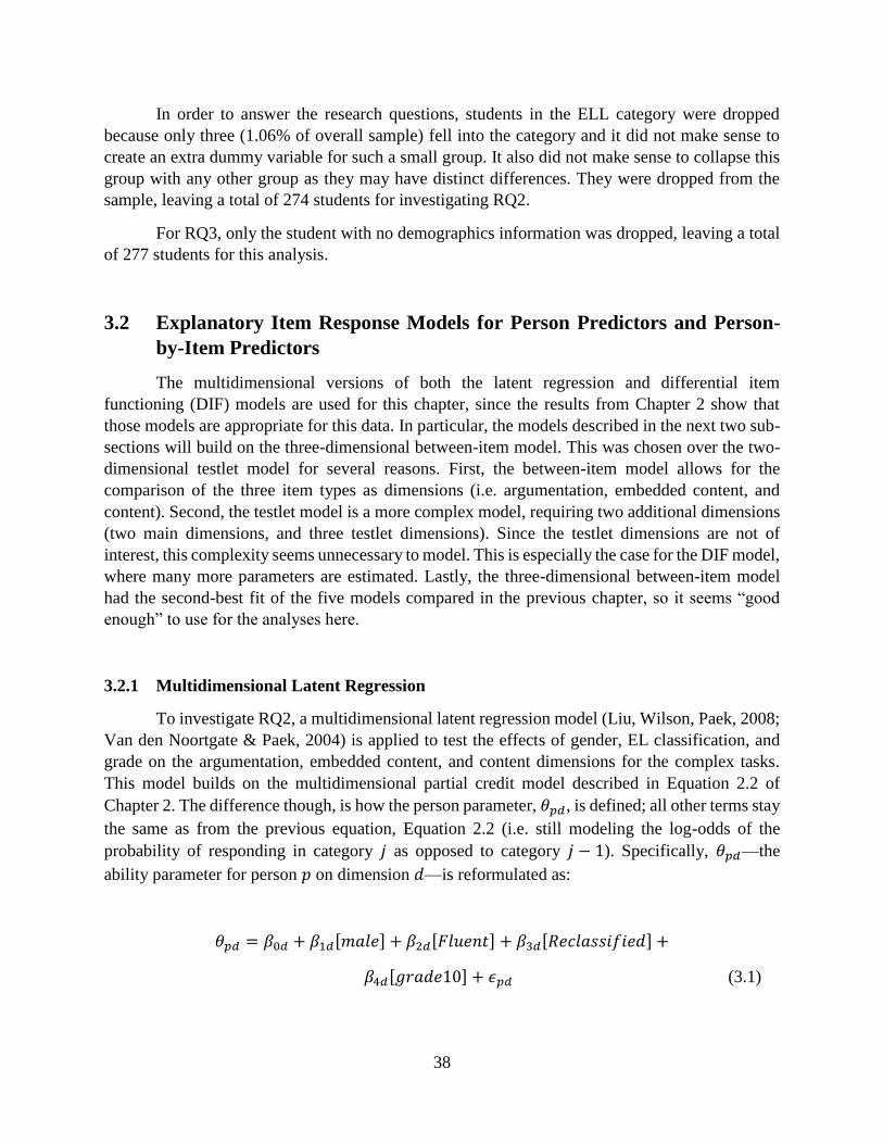
38

In order to answer the research questions, students in the ELL category were dropped

because only three (1.06% of overall sample) fell into the category and it did not make sense to

create an extra dummy variable for such a small group. It also did not make sense to collapse this

group with any other group as they may have distinct differences. They were dropped from the

sample, leaving a total of 274 students for investigating RQ2.

For RQ3, only the student with no demographics information was dropped, leaving a total

of 277 students for this analysis.

3.2 Explanatory Item Response Models for Person Predictors and Person-

by-Item Predictors

The multidimensional versions of both the latent regression and differential item

functioning (DIF) models are used for this chapter, since the results from Chapter 2 show that

those models are appropriate for this data. In particular, the models described in the next two sub-

sections will build on the three-dimensional between-item model. This was chosen over the two-

dimensional testlet model for several reasons. First, the between-item model allows for the

comparison of the three item types as dimensions (i.e. argumentation, embedded content, and

content). Second, the testlet model is a more complex model, requiring two additional dimensions

(two main dimensions, and three testlet dimensions). Since the testlet dimensions are not of

interest, this complexity seems unnecessary to model. This is especially the case for the DIF model,

where many more parameters are estimated. Lastly, the three-dimensional between-item model

had the second-best fit of the five models compared in the previous chapter, so it seems “good

enough” to use for the analyses here.

3.2.1 Multidimensional Latent Regression

To investigate RQ2, a multidimensional latent regression model (Liu, Wilson, Paek, 2008;

Van den Noortgate & Paek, 2004) is applied to test the effects of gender, EL classification, and

grade on the argumentation, embedded content, and content dimensions for the complex tasks.

This model builds on the multidimensional partial credit model described in Equation 2.2 of

Chapter 2. The difference though, is how the person parameter, 𝜃𝑝𝑑, is defined; all other terms stay

the same as from the previous equation, Equation 2.2 (i.e. still modeling the log-odds of the

probability of responding in category 𝑗 as opposed to category 𝑗 − 1). Specifically, 𝜃𝑝𝑑—the

ability parameter for person 𝑝 on dimension 𝑑—is reformulated as:

𝜃𝑝𝑑 = 𝛽0𝑑 + 𝛽1𝑑[𝑚𝑎𝑙𝑒] + 𝛽2𝑑[𝐹𝑙𝑢𝑒𝑛𝑡] + 𝛽3𝑑[𝑅𝑒𝑐𝑙𝑎𝑠𝑠𝑖𝑓𝑖𝑒𝑑] +

𝛽4𝑑[𝑔𝑟𝑎𝑑𝑒10] + 𝜖𝑝𝑑 (3.1)

39

where 𝜃𝑝𝑑 is regressed onto the dummy variables created for gender, EL classification, and grade,

respectively. The coefficient 𝛽1𝑑 represents the mean difference in ability between male and

female students on dimension 𝑑, after controlling for EL proficiency and grade. 𝛽2𝑑 and 𝛽3𝑑 are

the coefficients for students classified as “Fluent” and “Reclassified,” respectively, and they

represent the mean difference between these two groups and the reference group on dimension 𝑑,

after controlling for the other covariates. The reference group is composed of those students

classified as “English,” meaning that they speak only English at home. As noted above, students

classified as “English Language Learners” were dropped from the sample. 𝛽4𝑑 is the coefficient

for tenth graders, with eighth graders as the reference group. This coefficient represents the mean

difference between eighth and tenth graders on dimension 𝑑, after controlling for gender and EL

proficiency. 𝛽0𝑑 and 𝜖𝑝𝑑 represent the intercept and error terms for dimension 𝑑, respectively.

For this analysis, the three-dimensional between-item model was chosen as the

unconditional model (i.e. model with no covariates) for comparison. The final item parameters

from the three-dimensional between-item model from the previous chapter, after the delta

dimensional alignment was applied, were used as item anchors to estimate the conditional model

(model with the covariates or the multidimensional latent regression model)5. Using item

parameter estimates from the unconditional model as anchors are appropriate here, since generally

the conditional model will produce smaller standard errors even though there are negligible

differences in the item parameter estimates (Adams, Wilson, Wu, 1997; Wu, Adams, Wilson,

Haldane, 2007, pp.111-113).

By incorporating the covariates into this model, one can illustrate their effects on the three

item types (i.e. argumentation, embedded content, and content). In addition, by having the results

from both the unconditional and conditional models, the 𝑅2 can be calculated to see how much

additional variance is explained through the inclusion of these covariates.

3.2.2 Differential Item Functioning (DIF)

Differential item functioning (DIF) techniques are a variety of methods6 that seek to test

whether items have differential effects between the focal and reference groups. This chapter

focuses specifically on Rasch-based DIF methods to explore RQ3. These models involve

comparing two groups based on differences in the item parameters. Specifically, I build on

Equation 2.2, the multidimensional partial credit model. This updated equation can be written as:

5 In addition, the unconditional model was estimated again using the same anchored item parameters with the updated

sample. This was done so that the conditional model (model with regressors) can be compared directly to this

unconditional model, due to the small decrease in the sample with the removal of the ELL students and the student

with no demographic information. 6 Only the Rasch-based method will be described in detail here. For an overview of the different types of methods

available to test for DIF, readers should refer to Millsap & Everson (1993) and Osterlind & Everson (2009).

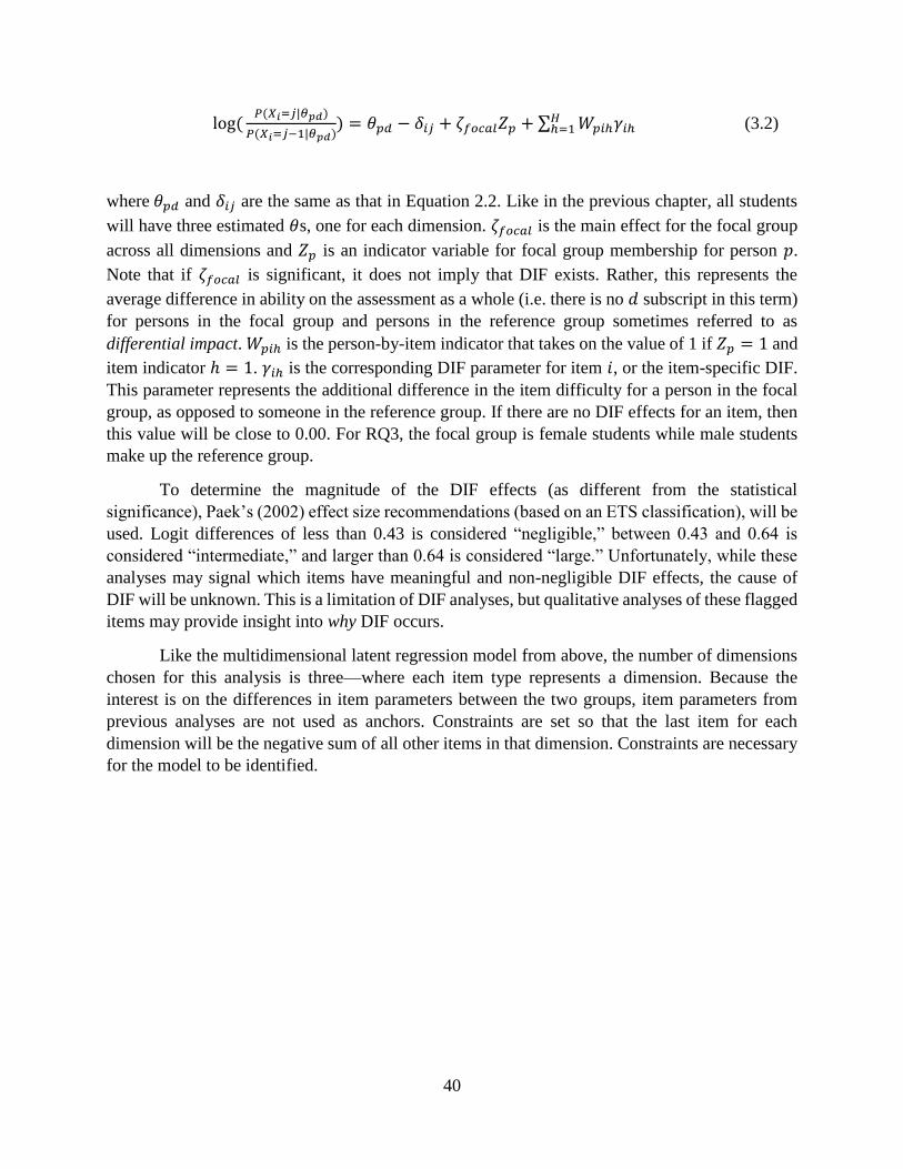
40

log(𝑃(𝑋𝑖=𝑗|𝜃𝑝𝑑)

𝑃(𝑋𝑖=𝑗−1|𝜃𝑝𝑑)) = 𝜃𝑝𝑑 − 𝛿𝑖𝑗 + 𝜁𝑓𝑜𝑐𝑎𝑙𝑍𝑝 + ∑ 𝑊𝑝𝑖ℎ𝛾𝑖ℎ

𝐻ℎ=1 (3.2)

where 𝜃𝑝𝑑 and 𝛿𝑖𝑗 are the same as that in Equation 2.2. Like in the previous chapter, all students

will have three estimated 𝜃s, one for each dimension. 𝜁𝑓𝑜𝑐𝑎𝑙 is the main effect for the focal group

across all dimensions and 𝑍𝑝 is an indicator variable for focal group membership for person 𝑝.

Note that if 𝜁𝑓𝑜𝑐𝑎𝑙 is significant, it does not imply that DIF exists. Rather, this represents the

average difference in ability on the assessment as a whole (i.e. there is no 𝑑 subscript in this term)

for persons in the focal group and persons in the reference group sometimes referred to as

differential impact. 𝑊𝑝𝑖ℎ is the person-by-item indicator that takes on the value of 1 if 𝑍𝑝 = 1 and

item indicator ℎ = 1. 𝛾𝑖ℎ is the corresponding DIF parameter for item 𝑖, or the item-specific DIF.

This parameter represents the additional difference in the item difficulty for a person in the focal

group, as opposed to someone in the reference group. If there are no DIF effects for an item, then

this value will be close to 0.00. For RQ3, the focal group is female students while male students

make up the reference group.

To determine the magnitude of the DIF effects (as different from the statistical

significance), Paek’s (2002) effect size recommendations (based on an ETS classification), will be

used. Logit differences of less than 0.43 is considered “negligible,” between 0.43 and 0.64 is

considered “intermediate,” and larger than 0.64 is considered “large.” Unfortunately, while these

analyses may signal which items have meaningful and non-negligible DIF effects, the cause of

DIF will be unknown. This is a limitation of DIF analyses, but qualitative analyses of these flagged

items may provide insight into why DIF occurs.

Like the multidimensional latent regression model from above, the number of dimensions

chosen for this analysis is three—where each item type represents a dimension. Because the

interest is on the differences in item parameters between the two groups, item parameters from

previous analyses are not used as anchors. Constraints are set so that the last item for each

dimension will be the negative sum of all other items in that dimension. Constraints are necessary

for the model to be identified.

41

3.3 Results

3.3.1 Latent Regression Results

Results from the multidimensional latent regression are shown in Table 3.1. The increase

in the 𝑅2, from using the conditional model as compared to the unconditional model, show that the

covariates explain more of the variance for the embedded content dimension than for the other two

dimensions. The increases in 𝑅2 are 37.62%, 26.62%, and 17.94% for the embedded content,

argumentation, and content dimensions, respectively.

The male students, on average, perform worse than female students by approximately 0.30

logit on the argumentation dimension after controlling for EL classification and grade. There is no

statistically significant difference between the genders on the other two dimensions. Not

surprisingly, tenth graders outperformed the eighth graders on all dimensions, after controlling for

El classification and gender. On average, they scored about 0.75, 1.14, and 0.94 logits higher than

eighth graders for the argumentation, embedded content, and content dimensions, respectively.

These differences were all statistically significant at an 𝛼 = 0.05 level.

For the EL classification groups, there were some notable differences in group means. The

reference group for this collection of covariates is students who only speak English at home. There

were no statistically significant differences between students classified as Fluent and those

classified as English in the argumentation and content dimensions. However, students classified

as Fluent performed about 0.44 logits higher on embedded content than those classified as English,

after controlling for gender and grade.

Students in the Reclassified group performed about 0.38 and 0.50 logits worse than the

English group on the argumentation and content dimensions, respectively, after controlling for

gender and grade. There were no statistically significant differences between the two groups on

the embedded content dimension.

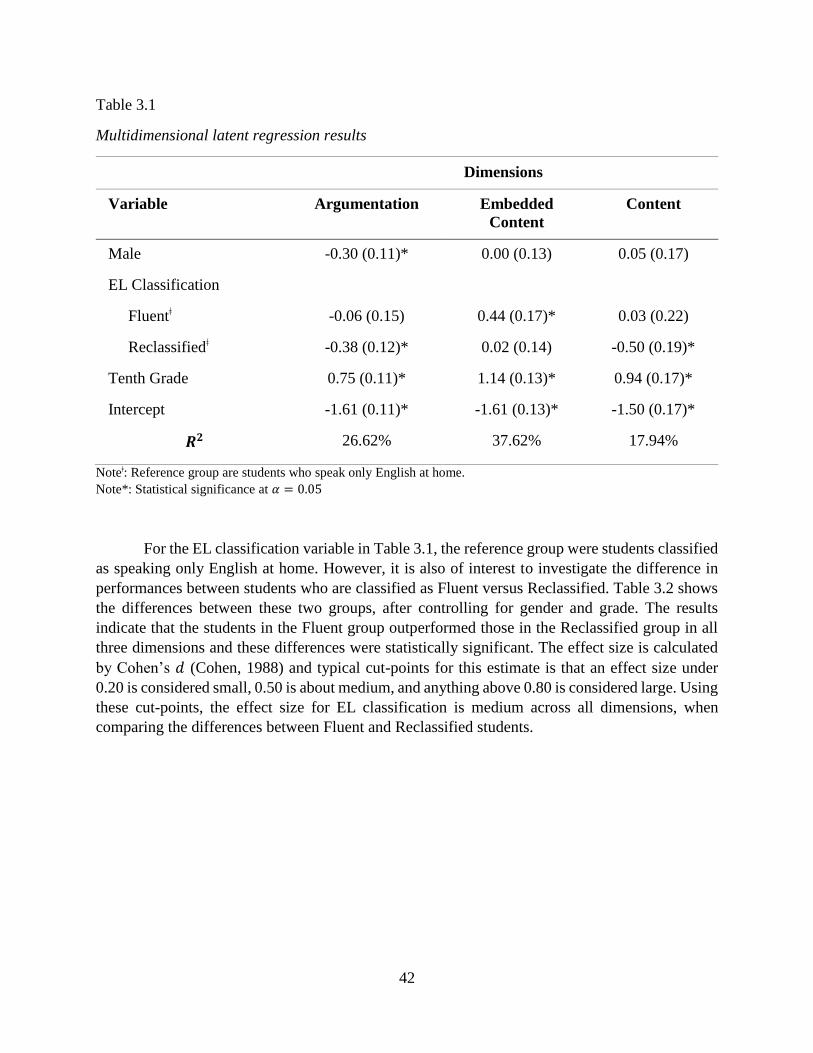
42

Table 3.1

Multidimensional latent regression results

Dimensions

Variable Argumentation Embedded

Content

Content

Male -0.30 (0.11)* 0.00 (0.13) 0.05 (0.17)

EL Classification

Fluentǂ -0.06 (0.15) 0.44 (0.17)* 0.03 (0.22)

Reclassifiedǂ -0.38 (0.12)* 0.02 (0.14) -0.50 (0.19)*

Tenth Grade 0.75 (0.11)* 1.14 (0.13)* 0.94 (0.17)*

Intercept -1.61 (0.11)* -1.61 (0.13)* -1.50 (0.17)*

𝑹𝟐 26.62% 37.62% 17.94%

Noteǂ: Reference group are students who speak only English at home.

Note*: Statistical significance at 𝛼 = 0.05

For the EL classification variable in Table 3.1, the reference group were students classified

as speaking only English at home. However, it is also of interest to investigate the difference in

performances between students who are classified as Fluent versus Reclassified. Table 3.2 shows

the differences between these two groups, after controlling for gender and grade. The results

indicate that the students in the Fluent group outperformed those in the Reclassified group in all

three dimensions and these differences were statistically significant. The effect size is calculated

by Cohen’s 𝑑 (Cohen, 1988) and typical cut-points for this estimate is that an effect size under

0.20 is considered small, 0.50 is about medium, and anything above 0.80 is considered large. Using

these cut-points, the effect size for EL classification is medium across all dimensions, when

comparing the differences between Fluent and Reclassified students.

43

Table 3.2

Post-hoc comparisons for students classified as Fluent and Reclassified

Dimension Difference in Means

(Fluent – Reclassified)

T p-value Effect Size*

Argumentation 0.32 (0.09) 3.39 0.001 0.48

Embedded Content 0.41 (0.10) 4.11 <0.001 0.53

Content 0.53 (0.15) 3.40 0.001 0.51

Note*: Effect size below 0.20 is small, 0.50 is medium, and 0.80 is high (Cohen, 1988).

Figures 3.1 to 3.3 provide a visual indication for the number of students by their EL

classification at each ability estimate for the argumentation, embedded content, and content

dimensions, respectively. Keep in mind that there were significantly fewer students in the Fluent

category than for the other two groups (58 students compared to 110 Reclassified and 106 English

students). In Figure 3.1, it is evident from the distributions that there are more of the English Only

and Fluent students at the higher end of the ability scale (around -1.20 to 0.50 logit). The

Reclassified students cluster near the middle (around -2.00 to -1.00 logit).

In Figure 3.2, it is more difficult to distinguish between the differences for Reclassified

and English Only students. Their patterns seem similar with both distributions having multiple

peaks between -1.50 to 0.00 logit. However, there were more Fluent students clustered at the upper

end of the distribution. These results confirm the findings from Table 3.1, where no significant

differences were found between the English Only and Reclassified groups. However, both of these

groups performed statistically significantly worse than the students classified as Fluent.

Lastly, the distributions of students in the three English proficiency groups on the content

dimension are shown in Figure 3.3. The Reclassified group have a few students at the lowest end

of the ability distribution, and very few at the top end. Reclassified students performed about half

a logit worse than both the English Only and the Fluent students, on average, after controlling for

gender and grade. There were no statistically significant differences between the English Only and

the Fluent students, and their distributions take on a similar shape.

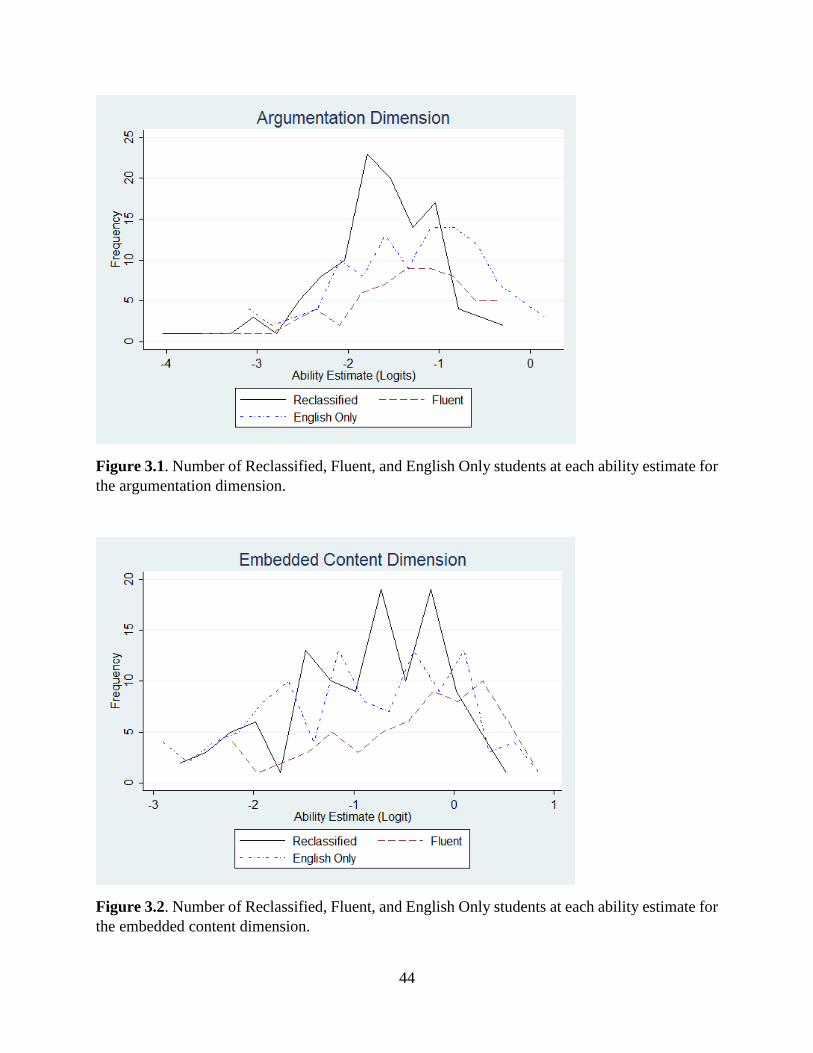
44

Figure 3.1. Number of Reclassified, Fluent, and English Only students at each ability estimate for

the argumentation dimension.

Figure 3.2. Number of Reclassified, Fluent, and English Only students at each ability estimate for

the embedded content dimension.

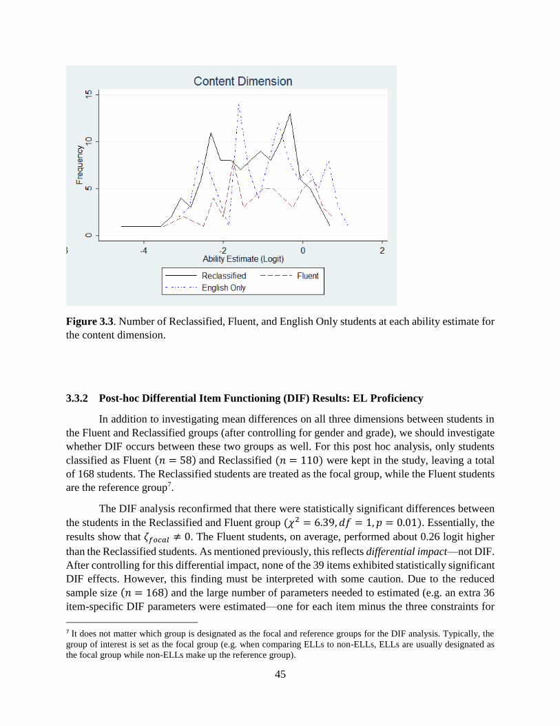
45

Figure 3.3. Number of Reclassified, Fluent, and English Only students at each ability estimate for

the content dimension.

3.3.2 Post-hoc Differential Item Functioning (DIF) Results: EL Proficiency

In addition to investigating mean differences on all three dimensions between students in

the Fluent and Reclassified groups (after controlling for gender and grade), we should investigate

whether DIF occurs between these two groups as well. For this post hoc analysis, only students

classified as Fluent (𝑛 = 58) and Reclassified (𝑛 = 110) were kept in the study, leaving a total

of 168 students. The Reclassified students are treated as the focal group, while the Fluent students

are the reference group7.

The DIF analysis reconfirmed that there were statistically significant differences between

the students in the Reclassified and Fluent group (𝜒2 = 6.39, 𝑑𝑓 = 1, 𝑝 = 0.01). Essentially, the

results show that 𝜁𝑓𝑜𝑐𝑎𝑙 ≠ 0. The Fluent students, on average, performed about 0.26 logit higher

than the Reclassified students. As mentioned previously, this reflects differential impact—not DIF.

After controlling for this differential impact, none of the 39 items exhibited statistically significant

DIF effects. However, this finding must be interpreted with some caution. Due to the reduced

sample size (𝑛 = 168) and the large number of parameters needed to estimated (e.g. an extra 36

item-specific DIF parameters were estimated—one for each item minus the three constraints for

7 It does not matter which group is designated as the focal and reference groups for the DIF analysis. Typically, the

group of interest is set as the focal group (e.g. when comparing ELLs to non-ELLs, ELLs are usually designated as

the focal group while non-ELLs make up the reference group).

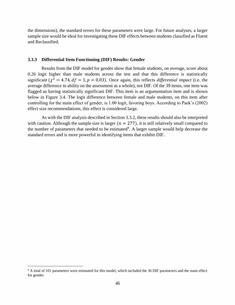
46

the dimensions), the standard errors for these parameters were large. For future analyses, a larger

sample size would be ideal for investigating these DIF effects between students classified as Fluent

and Reclassified.

3.3.3 Differential Item Functioning (DIF) Results: Gender

Results from the DIF model for gender show that female students, on average, score about

0.26 logit higher than male students across the test and that this difference is statistically

significant (𝜒2 = 4.74, 𝑑𝑓 = 1, 𝑝 = 0.03). Once again, this reflects differential impact (i.e. the

average difference in ability on the assessment as a whole), not DIF. Of the 39 items, one item was

flagged as having statistically significant DIF. This item is an argumentation item and is shown

below in Figure 3.4. The logit difference between female and male students, on this item after

controlling for the main effect of gender, is 1.00 logit, favoring boys. According to Paek’s (2002)

effect size recommendations, this effect is considered large.

As with the DIF analysis described in Section 3.3.2, these results should also be interpreted

with caution. Although the sample size is larger (𝑛 = 277), it is still relatively small compared to

the number of parameters that needed to be estimated8. A larger sample would help decrease the

standard errors and is more powerful in identifying items that exhibit DIF.

8 A total of 101 parameters were estimated for this model, which included the 36 DIF parameters and the main effect

for gender.

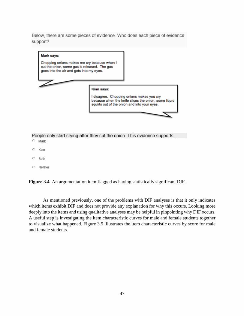
47

Figure 3.4. An argumentation item flagged as having statistically significant DIF.

As mentioned previously, one of the problems with DIF analyses is that it only indicates

which items exhibit DIF and does not provide any explanation for why this occurs. Looking more

deeply into the items and using qualitative analyses may be helpful in pinpointing why DIF occurs.

A useful step is investigating the item characteristic curves for male and female students together

to visualize what happened. Figure 3.5 illustrates the item characteristic curves by score for male

and female students.

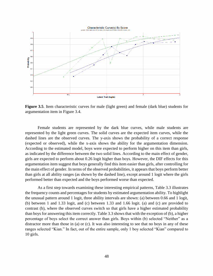
48

Figure 3.5. Item characteristic curves for male (light green) and female (dark blue) students for

argumentation item in Figure 3.4.

Female students are represented by the dark blue curves, while male students are

represented by the light green curves. The solid curves are the expected item curves, while the

dashed lines are the observed curves. The y-axis shows the probability of a correct response

(expected or observed), while the x-axis shows the ability for the argumentation dimension.

According to the estimated model, boys were expected to perform higher on this item than girls,

as indicated by the difference between the two solid lines. According to the main effect of gender,

girls are expected to perform about 0.26 logit higher than boys. However, the DIF effects for this

argumentation item suggest that boys generally find this item easier than girls, after controlling for

the main effect of gender. In terms of the observed probabilities, it appears that boys perform better

than girls at all ability ranges (as shown by the dashed line), except around 1 logit where the girls

performed better than expected and the boys performed worse than expected.

As a first step towards examining these interesting empirical patterns, Table 3.3 illustrates

the frequency counts and percentages for students by estimated argumentation ability. To highlight

the unusual pattern around 1 logit, three ability intervals are shown: (a) between 0.66 and 1 logit,

(b) between 1 and 1.33 logit, and (c) between 1.33 and 1.66 logit. (a) and (c) are provided to

contrast (b), where the observed curves switch so that girls have a higher estimated probability

than boys for answering this item correctly. Table 3.3 shows that with the exception of (b), a higher

percentage of boys select the correct answer than girls. Boys within (b) selected “Neither” as a

distractor more than those in (a) or (c). It was also interesting to see that no boys in any of these

ranges selected “Kian.” In fact, out of the entire sample, only 1 boy selected “Kian” compared to

10 girls.

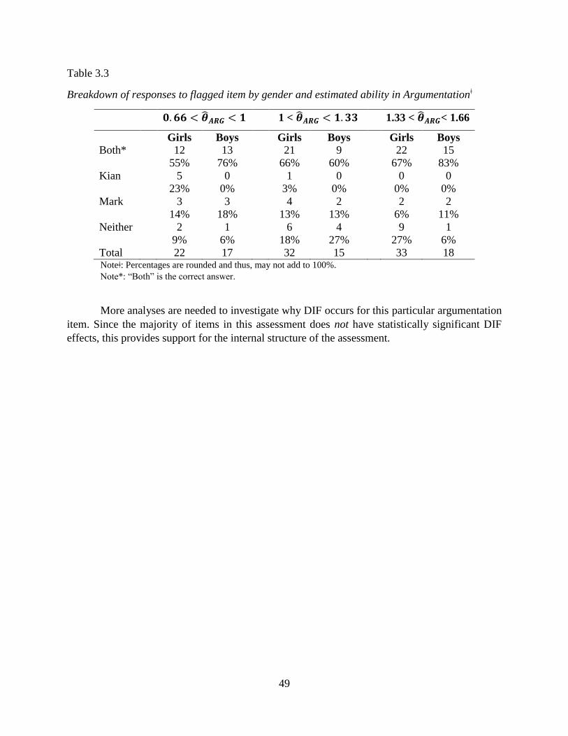
49

Table 3.3

Breakdown of responses to flagged item by gender and estimated ability in Argumentationǂ

𝟎. 𝟔𝟔 < �̂�𝑨𝑹𝑮 < 𝟏 1 < �̂�𝑨𝑹𝑮 < 𝟏. 𝟑𝟑 1.33 < �̂�𝑨𝑹𝑮< 1.66

Girls Boys Girls Boys Girls Boys

Both* 12

55%

13

76%

21

66%

9

60%

22

67%

15

83%

Kian 5

23%

0

0%

1

3%

0

0%

0

0%

0

0%

Mark 3

14%

3

18%

4

13%

2

13%

2

6%

2

11%

Neither 2

9%

1

6%

6

18%

4

27%

9

27%

1

6%

Total 22 17 32 15 33 18 Noteǂ: Percentages are rounded and thus, may not add to 100%.

Note*: “Both” is the correct answer.

More analyses are needed to investigate why DIF occurs for this particular argumentation

item. Since the majority of items in this assessment does not have statistically significant DIF

effects, this provides support for the internal structure of the assessment.

50

3.4. Discussion and Future Steps

This chapter applies two different types of EIRMs to the LPS data, the multidimensional

latent regression model and a Rasch-based DIF model, in an attempt to explain performance on

the assessment using person predictors and person-by-item predictors, respectively. The results

from these models also provide validity evidence for the assessment.

For the multidimensional latent regression model, several person predictors were used to

investigate performance on the items, including gender, EL proficiency, and grade. As one might

well have expected, grade was a statistically significant predictor across all dimensions, after

controlling for the other covariates. This finding makes sense as tenth graders generally have more

content knowledge and experience in argumentation, and in taking assessments than eighth

graders—making it likely that they would outperform eighth graders on all of the tasks.

Gender was a statistically significant predictor only on the argumentation dimension. This

supports the findings by Asterhan, Schwarz, & Gil (2012) that all-female groups provided higher

quality arguments than their all-male counterparts. However, other studies have suggested no

significant gender difference for argumentation (Naylor, Keogh, & Downing, 2007; Wilson,

Taylor, Kowalski, & Carlson, 2009). The lack of a significant difference in the content and

embedded content dimensions supports the research literature, where it has generally been shown

that female students in middle school grades tend to perform just as well as male students in science

(Catsambis, 1995; Hyde & Linn, 2006; Weinburg, 1995).

EL classifications also had statistically significant results for the latent regression. When

comparing students classified as Fluent and English, the performance on the embedded content

dimension differed—favoring those classified as Fluent. Both of these groups are fluent in English,

so it was surprising to see a difference. However, not much is known about these embedded content

items and this finding should be reinvestigated with new data to learn more about this relationship.

When comparing Reclassified students with English students, the Reclassified students

performed worse on the argumentation and content dimensions—with no significant estimated

differences in the embedded content dimensions. While it is unsurprising that the Reclassified

students performed worse on the two dimensions, it is informative to know that there were no

differences on the embedded content dimension. English Only students may have also had

difficulties with these items that did not resemble traditional science items.

The post hoc analyses revealed that the Reclassified students consistently performed worse

on all three dimensions than the Fluent students, after controlling for grade and gender. Even

though both groups of students speak a language other than English at home, Reclassified students

were, at one point, classified as ELLs who traditionally performed worse on assessments. It is

unsurprising that they performed worse than the Fluent students across all the dimensions. In

addition, a follow-up DIF analysis revealed no statistically significant DIF effects for Reclassified

and Fluent students. This result suggests no interaction effects and provides evidence for the

internal structure of the assessment.

51

For RQ3, a DIF analysis comparing male and female students identified only one item as

having statistically significant DIF effects, thereby providing additional validity evidence for the

internal structure of the LPS assessment. This was an argumentation item that heavily favored the

male students. Just as for many DIF analyses, the cause of DIF for this item is unknown (i.e. we

do not know why boys found this item easier), although speculation is possible, especially when

supported by more detailed analyses. Future studies using additional approaches may help explain

why DIF occurs, such as the model proposed by Xie and Wilson (2008) where they proposed a

differential facets functioning model. Rather than test person-by-item effects, they tested person-

by-facets effects. In order to run this model, theories into what might be the cause of DIF are

needed a priori.

While the analyses described in this chapter were informative, there were limitations to

their interpretability. First, the sample size proved to be problematic, especially with detecting DIF

as the standard errors were somewhat large. Future analyses should include a much larger sample

size for a more powerful DIF analysis.

Related to the small sample size problem, there were very few students classified as ELLs9.

While this could have simply reflected the lack of ELLs in the classrooms sampled, another

possibility is that students are often reclassified out of the ELL category in the upper grades even

if they do not meet the proficiency standards (Abedi, 2008). A more diverse and representative

sample, encompassing a larger grade range, would be ideal for reinvestigating this assessment.

The previous chapter provided evidence for the multidimensional structure of the LPS

assessment. This chapter focused on the person side of the Rasch partial credit model by testing

person predictors and the interaction of these person characteristics with specific items. However,

what can be learned from the item features? The next chapter examines the role of item predictors

and its effectiveness in explaining student performance on these items.

9 Abedi (2008) has also discussed problems with the overall EL classification system in the U.S., which typically

consists of a home language survey and English proficiency tests. These problems include inconsistencies in defining

“English Language Learner”, difference in standards across states, as well as problems with the language surveys and

proficiency tests themselves.

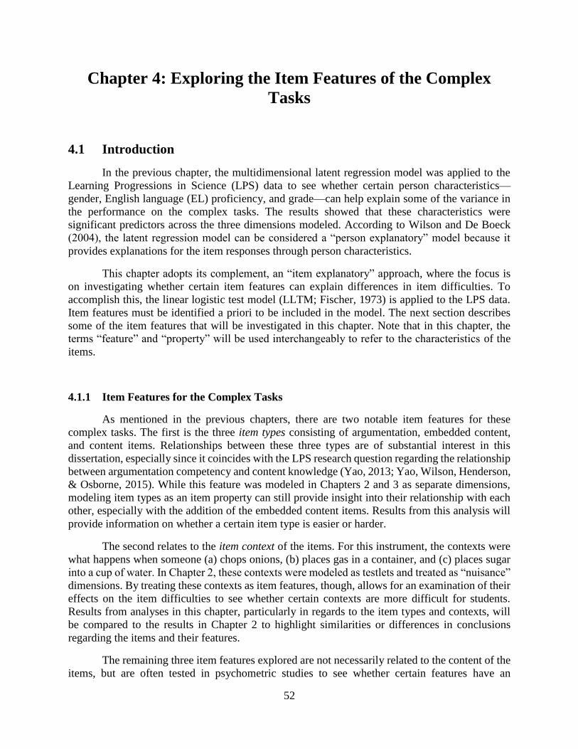
52

Chapter 4: Exploring the Item Features of the Complex

Tasks

4.1 Introduction

In the previous chapter, the multidimensional latent regression model was applied to the

Learning Progressions in Science (LPS) data to see whether certain person characteristics—

gender, English language (EL) proficiency, and grade—can help explain some of the variance in

the performance on the complex tasks. The results showed that these characteristics were

significant predictors across the three dimensions modeled. According to Wilson and De Boeck

(2004), the latent regression model can be considered a “person explanatory” model because it

provides explanations for the item responses through person characteristics.

This chapter adopts its complement, an “item explanatory” approach, where the focus is

on investigating whether certain item features can explain differences in item difficulties. To

accomplish this, the linear logistic test model (LLTM; Fischer, 1973) is applied to the LPS data.

Item features must be identified a priori to be included in the model. The next section describes

some of the item features that will be investigated in this chapter. Note that in this chapter, the

terms “feature” and “property” will be used interchangeably to refer to the characteristics of the

items.

4.1.1 Item Features for the Complex Tasks

As mentioned in the previous chapters, there are two notable item features for these

complex tasks. The first is the three item types consisting of argumentation, embedded content,

and content items. Relationships between these three types are of substantial interest in this

dissertation, especially since it coincides with the LPS research question regarding the relationship

between argumentation competency and content knowledge (Yao, 2013; Yao, Wilson, Henderson,

& Osborne, 2015). While this feature was modeled in Chapters 2 and 3 as separate dimensions,

modeling item types as an item property can still provide insight into their relationship with each

other, especially with the addition of the embedded content items. Results from this analysis will

provide information on whether a certain item type is easier or harder.

The second relates to the item context of the items. For this instrument, the contexts were

what happens when someone (a) chops onions, (b) places gas in a container, and (c) places sugar

into a cup of water. In Chapter 2, these contexts were modeled as testlets and treated as “nuisance”

dimensions. By treating these contexts as item features, though, allows for an examination of their

effects on the item difficulties to see whether certain contexts are more difficult for students.

Results from analyses in this chapter, particularly in regards to the item types and contexts, will

be compared to the results in Chapter 2 to highlight similarities or differences in conclusions

regarding the items and their features.

The remaining three item features explored are not necessarily related to the content of the

items, but are often tested in psychometric studies to see whether certain features have an

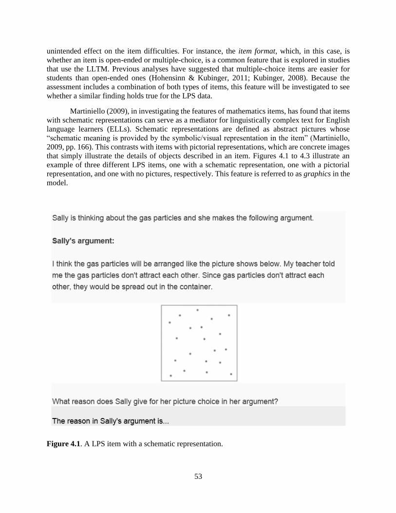
53

unintended effect on the item difficulties. For instance, the item format, which, in this case, is

whether an item is open-ended or multiple-choice, is a common feature that is explored in studies

that use the LLTM. Previous analyses have suggested that multiple-choice items are easier for

students than open-ended ones (Hohensinn & Kubinger, 2011; Kubinger, 2008). Because the

assessment includes a combination of both types of items, this feature will be investigated to see

whether a similar finding holds true for the LPS data.

Martiniello (2009), in investigating the features of mathematics items, has found that items

with schematic representations can serve as a mediator for linguistically complex text for English

language learners (ELLs). Schematic representations are defined as abstract pictures whose

“schematic meaning is provided by the symbolic/visual representation in the item” (Martiniello,

2009, pp. 166). This contrasts with items with pictorial representations, which are concrete images

that simply illustrate the details of objects described in an item. Figures 4.1 to 4.3 illustrate an

example of three different LPS items, one with a schematic representation, one with a pictorial

representation, and one with no pictures, respectively. This feature is referred to as graphics in the

model.

Figure 4.1. A LPS item with a schematic representation.

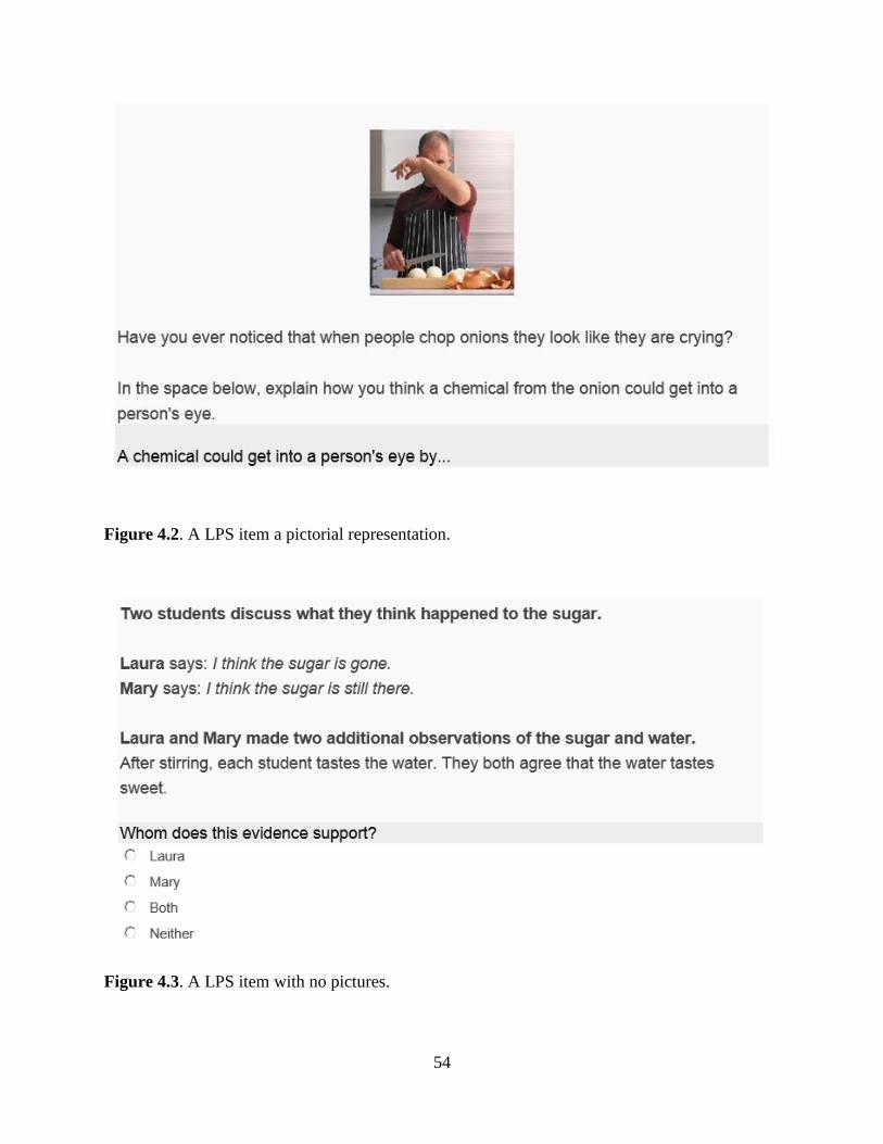
54

Figure 4.2. A LPS item a pictorial representation.

Figure 4.3. A LPS item with no pictures.

55

The last feature investigated is whether an item contains academic words. Academic

vocabulary words are those that are not among the 2,000 most common words and occur most

often in academic texts (Coxhead, 2000). Unlike technical vocabulary—which are the specialized

words specific to a discipline, academic vocabulary words are more generalized and span across

many content areas (Stevens, Butler, & Castellon-Wellington, 2001). This distinction is important

for many studies investigating the language effects of content assessments—particularly for

ELLs—because, while technical vocabulary is deemed to be construct-relevant, academic

vocabulary is often seen as construct-irrelevant and, subsequently, may interfere with the

interpretations of student scores on assessments (Avenia-Tapper & Llosa, 2015; Haag, Roppelt, &

Heppt, 2015; Wolf and Leon, 2009). In this chapter, the focus is on the occurrence of academic

words, not the specialized technical vocabulary, to test whether there are some extraneous

construct-irrelevant effects. That is, do academic words contribute significantly to the difficulty of

an item? Coxhead’s (2000) academic word list (AWL) is used here to identify academic words on

the assessment10. Note that the word “evidence” is on the AWL, but will not be counted as an

academic word in this chapter because “evidence” is central to the argumentation construct. Thus,

“evidence” can be thought of as construct-relevant, whereas other words on the AWL may be

considered construct-irrelevant. In the model, this feature will be referred to as AWL.

4.1.2 Research Questions

This chapter explores the effect of each item feature on overall item difficulty. A total of

five item features is investigated for this chapter, including: type, context, format, graphics, and

AWL. Specifically, the research questions are listed below:

RQ4. Which of the following, if any, item features—type, context, format, inclusion of graphics,

and inclusion of vocabulary from the Academic Word List—contribute to the explanation

of item difficulty?

RQ5. Does the item type feature interact with any of the other features to have a statistically

significant effect on the item difficulties?

To investigate RQ4 and RQ5, the LLTM (see below for an introduction to the LLTM) is

applied to the data using the five item features described in the previous section. For RQ5,

interactions are included in the model—focusing on the item type. Because of the added

complexities in interpreting interactions, only one feature was explored in further detail. Item type

was chosen because it directly relates to the content of the items. Plus, as mentioned earlier, the

10 Cobb’s website Web Vocabprofile Classic at http://www.lextutor.ca/vp/eng/ automatically sorts texts and provides

counts for four types of words: the 1000 most frequent words, 1001-2000 most frequent words, words on Coxhead’s

(2000) Academic Word List, and off-list words.

56

three item types are related to the main research questions for the LPS project. Thus, investigating

interactions of item types with the other features can provide more information as to how this

feature influences item difficulty. In addition, the models in these two research questions are

nested, allowing for direct comparisons via a likelihood ratio test to find the better fitting model.

These models will also be compared to the unidimensional partial credit model from Chapter 2 to

see how well the models from RQ4 and RQ5 can recover these estimated item difficulties. If the

item features related to the construct of interest (i.e. type) are selected and found to help predict

item difficulty, then this can contribute evidence supporting the construct validity of the

assessment (Embretson, 1983; Hartig, Frey, Nold, & Klieme, 2011).

4.2 Explanatory Item Response Models for Item Features

4.2.1 The Linear Logistic Test Model and Its Extensions

The linear logistic test model (LLTM; Fischer, 1973) decomposes the item difficulty into

a linear combination of item features. Because the items in the LPS data are polytomously scored,

the extension for the LLTM is described here. This extension is sometimes referred to as the linear

partial credit model (Fischer & Ponocny, 1994) which is also similar to the multifacet Rasch model

(Linacre, 1989). This model builds off the partial credit model, which was shown in Equation 2.1.

The difference, though, is how 𝛿𝑖𝑗 is modeled; all other terms stay the same (i.e. 𝜃𝑝 is the ability

for person 𝑝 and we are still modelling the log-odds of the probability of responding in

category 𝑗 as opposed to category 𝑗 − 1). 𝛿𝑖𝑗 is defined as:

𝛿𝑖𝑗 = ∑ 𝛽𝑚𝑋𝑖𝑗𝑚𝑀𝑚=1 (4.1)

where 𝑋𝑖𝑗𝑚 is the value for step 𝑗 of item 𝑖 on feature 𝑚 and 𝛽𝑚 is the regression weight for item

feature 𝑚. Unlike in the previous two chapters, however, a multidimensional approach is not taken

here. Notice that the item step parameter, 𝛿𝑖𝑗 from Equation 2.1, is replaced with the linear

combination of the difficulties of the item features, rather than the individual item difficulties.

To answer RQ4, which is to investigate the effects of certain item features on item

difficulty, the overall item difficulty across the steps can be written as:

𝛿𝑖𝑜𝑣𝑒𝑟𝑎𝑙𝑙 = 𝛽1𝑡𝑦𝑝𝑒𝑖 + 𝛽2𝑡𝑎𝑠𝑘𝑖 + 𝛽3𝑓𝑜𝑟𝑚𝑎𝑡𝑖 + 𝛽4𝑔𝑟𝑎𝑝ℎ𝑖𝑐𝑠𝑖 + 𝛽5𝐴𝑊𝐿𝑖 (4.2)

57

where the coefficients for each feature determines if the item becomes easier or more difficult.

That is, the overall item difficulty is calculated by adding the estimated coefficients for each

feature. Thus, items with the same features are predicted to have the exact same item difficulty.

For RQ5, interaction effects are added to Equation 4.2. As an example, Equation 4.3 shows the

overall item difficulty for a model that includes interaction terms for type and all other features.

𝛿𝑖𝑜𝑣𝑒𝑟𝑎𝑙𝑙 = 𝛽1𝑡𝑦𝑝𝑒𝑖 + 𝛽2𝑡𝑎𝑠𝑘𝑖 + 𝛽3𝑓𝑜𝑟𝑚𝑎𝑡𝑖 + 𝛽4𝑔𝑟𝑎𝑝ℎ𝑖𝑐𝑠𝑖 + 𝛽5𝐴𝑊𝐿𝑖 + 𝛽6𝑡𝑦𝑝𝑒𝑖 ∗ 𝑡𝑎𝑠𝑘𝑖 +

𝛽7𝑡𝑦𝑝𝑒𝑖 ∗ 𝑓𝑜𝑟𝑚𝑎𝑡𝑖 + 𝛽8𝑡𝑦𝑝𝑒𝑖 ∗ 𝑔𝑟𝑎𝑝ℎ𝑖𝑐𝑠𝑖 + 𝛽9𝑡𝑦𝑝𝑒𝑖 ∗ 𝐴𝑊𝐿𝑖 (4.3)

Because Equation 4.2 can be found by constraining some of the parameters in Equation 4.3

(i.e. 𝛽𝑘 = 0, for 𝑘 > 5), these two models can be directly compared using a likelihood ratio test.

In addition, both these models are nested within the partial credit model. All three models will be

compared directly and also with the model fit statistics AIC and BIC, as in previous chapters.

4.3 Results

4.3.1. Descriptive Statistics

Table 4.1 provides the frequencies for each of the five item features on the LPS assessment.

Recall that the test included a total of 39 items. For the item type, the items are not distributed

evenly across the three categories. Argumentation items make up approximately half of the items,

while only 17.95% of the items are categorized as embedded content. On the other hand, the items

are about evenly distributed for the item contexts, format, and graphics. Only 13 items, or 33.33%,

contained academic words.

58

Table 4.1

Frequencies for Each Item Feature on the LPS Assessment

Item Feature Count Percentage

Type

Argumentation 20 51.28

Embedded Content 7 17.95

Content 12 30.77

Context

Sugar 12 30.77

Onions 14 35.90

Gases 13 33.33

Format

Multiple-Choice 19 48.72

Open-Ended 20 51.28

Graphics

Schematic 11 28.21

Pictorial 14 35.90

None 14 35.90

Academic Words List (AWL)

Yes* 13 33.33

No 26 66.67

Note*: “Yes” means that an item contains at least one AWL word. It does not account for the number of AWL words

in an item.

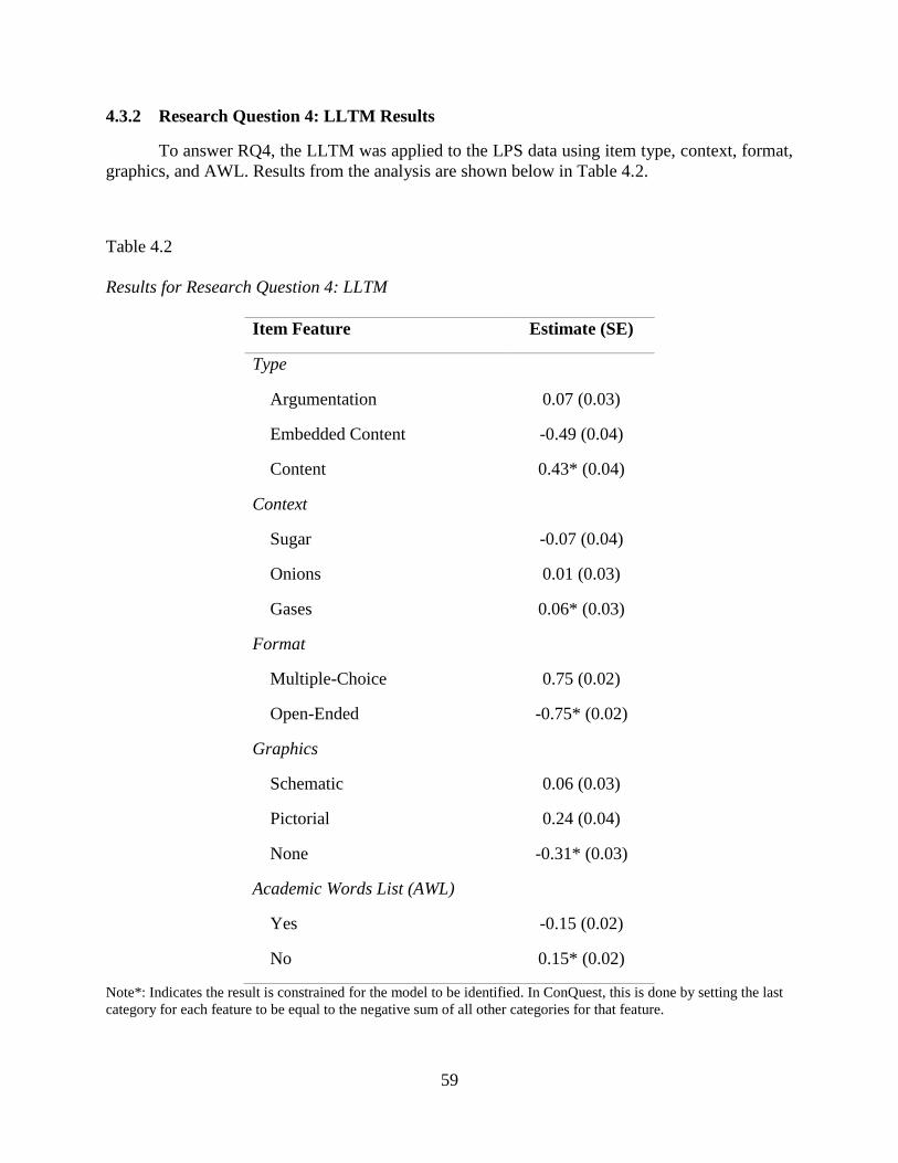
59

4.3.2 Research Question 4: LLTM Results

To answer RQ4, the LLTM was applied to the LPS data using item type, context, format,

graphics, and AWL. Results from the analysis are shown below in Table 4.2.

Table 4.2

Results for Research Question 4: LLTM

Item Feature Estimate (SE)

Type

Argumentation 0.07 (0.03)

Embedded Content -0.49 (0.04)

Content 0.43* (0.04)

Context

Sugar -0.07 (0.04)

Onions 0.01 (0.03)

Gases 0.06* (0.03)

Format

Multiple-Choice 0.75 (0.02)

Open-Ended -0.75* (0.02)

Graphics

Schematic 0.06 (0.03)

Pictorial 0.24 (0.04)

None -0.31* (0.03)

Academic Words List (AWL)

Yes -0.15 (0.02)

No 0.15* (0.02)

Note*: Indicates the result is constrained for the model to be identified. In ConQuest, this is done by setting the last

category for each feature to be equal to the negative sum of all other categories for that feature.

60

For the item type feature, the embedded content items were estimated to be the easiest,

while the content items were identified as the most difficult. Argumentation items lie somewhere

in between. The chi-square test of parameter equality is statistically significant (𝜒2 =175.30 𝑑𝑓 = 2, 𝑝 < 0.001), suggesting that there is variation across these types. The mean-

squares value was 1.85 for the embedded content feature, suggesting that this features was not

fitting the data well. Typically, mean-square values less than 0.75 and larger than 1.33 signal misfit

(Adams & Khoo, 1996; Wilson, 2005). The large mean-square value for the embedded content

may be a result of simply too few data points (there were only seven embedded content items).

However, this needs further investigation. The other two features have acceptable mean-squares

values.

The variation between the item context features, on the other hand, is much smaller—

maybe even non-existent. The estimates for these three contexts are so similar that their confidence

intervals all overlap. This is confirmed by the chi-square test of parameter equality (𝜒2 =4.37 𝑑𝑓 = 2, 𝑝 = 0.11). These results suggest that the item contexts do not vary in their difficulty.

This finding is reassuring since the interest was never on how well students perform on items about

sugar or onions, but rather on the types of items.

Surprisingly, the multiple-choice feature was estimated to increase the difficulty of an item

by approximately 0.75 logit whereas the open-ended feature was estimated to decrease the

difficulty by 0.75 logit. The fit statistics for the open-ended feature was large (MNSQ=1.44), while

it was acceptable for the multiple-choice feature (MNSQ=0.86). These results suggest that there

were greater variations among the open-ended items than in the multiple-choice items, which may

explain the odd result. As an example, Figure 4.4 shows the Wright Map with the partial credit

difficulty estimates (from Chapter 2) by multiple-choice (blue) and open-ended (red) items11. The

map shows that the variation in estimated item difficulty is greater for the open-ended than for

multiple-choice items. While there are easy multiple-choice and open-ended items, the two most

difficult items are open-ended. Some open-ended items just required students to “identify a claim”

which is a level 0b item on the argumentation construct map. Other items require students to

“explain how the evidence supports your answer,” which is a level 2a argumentation item.

Obviously, these two open-ended items should differ in their difficulty—the first is simply writing

down a claim while the latter requires a more thoughtful explanation. These differences are not

accounted for in the LLTM and shows some of the limitations of decomposing item difficulties

into only a handful of features.

11 Note that, overall, most items were easy for this sample of students. The distribution of student abilities are generally

higher than the distribution for the item difficulties as seen in the Wright Map (Figure 4.4).

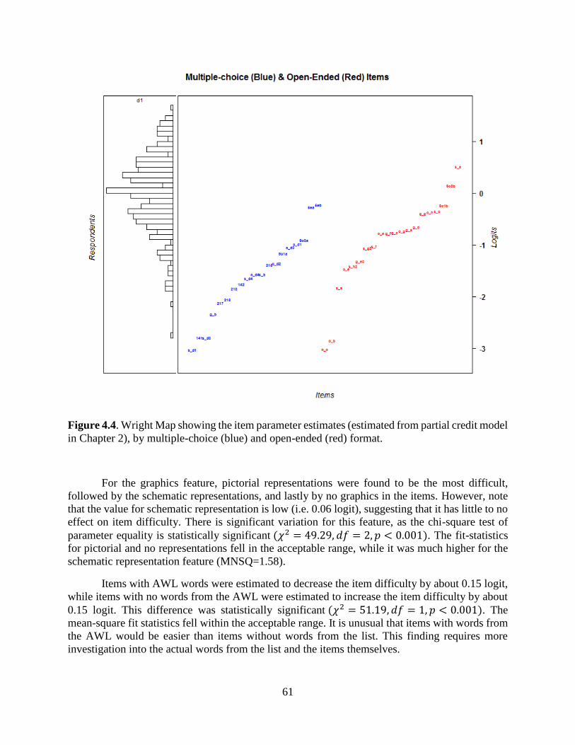
61

Figure 4.4. Wright Map showing the item parameter estimates (estimated from partial credit model

in Chapter 2), by multiple-choice (blue) and open-ended (red) format.

For the graphics feature, pictorial representations were found to be the most difficult,

followed by the schematic representations, and lastly by no graphics in the items. However, note

that the value for schematic representation is low (i.e. 0.06 logit), suggesting that it has little to no

effect on item difficulty. There is significant variation for this feature, as the chi-square test of

parameter equality is statistically significant (𝜒2 = 49.29, 𝑑𝑓 = 2, 𝑝 < 0.001). The fit-statistics

for pictorial and no representations fell in the acceptable range, while it was much higher for the

schematic representation feature (MNSQ=1.58).

Items with AWL words were estimated to decrease the item difficulty by about 0.15 logit,

while items with no words from the AWL were estimated to increase the item difficulty by about

0.15 logit. This difference was statistically significant (𝜒2 = 51.19, 𝑑𝑓 = 1, 𝑝 < 0.001). The

mean-square fit statistics fell within the acceptable range. It is unusual that items with words from

the AWL would be easier than items without words from the list. This finding requires more

investigation into the actual words from the list and the items themselves.

62

One way to explore this finding further is to calculate the reading difficulty of items with

AWL and those without. Here, the Flesch-Kincaid Readability index (Flesch, 1951; Kincaid,

Fishburne, Rogers, & Chissom, 1975) was used. While there are plenty of other readability

formulas available (Klare, 1984), the Flesch-Kincaid is one of the most popular and easily

accessible automated indices. For this post-hoc analysis, the Flesch-Kincaid was derived using

Microsoft Word 2013. It provides the reading level for a selected passage—in this case, the item.

The average grade level for the items with AWL words is 6.69, compared to 5.07 for those without.

This is about a 1.62 grade level difference, suggesting that the items with AWL words are more

difficult to read. However, the sample includes eighth and tenth graders, so the average readability

of all the items are well below their grades and may explain why items with AWL words are not

any more difficult.

4.3.3 Research Question 5: LLTM with Interactions Results

To answer RQ5, a LLTM with interactions model was also applied to the LPS data.

Because the context item feature was not statistically significant from the simple LLTM, it was

excluded from this model. Two interaction terms were generated for the features: type*format and

type*AWL. Interactions between types with graphics were not modeled because all embedded

content items had some sort of graphic representation accompanying them and none of the content

items had pictorial representations. The results are shown below in Table 4.3.

The interaction term type*format was statistically significant (𝜒2 = 51.03, 𝑑𝑓 = 2, 𝑝 <0.001). Multiple-choice embedded content items contribute an additional 0.26 logit to the item

difficulty, while multiple-choice content items contribute an additional -0.25 logit to the item

difficulty. For argumentation items, it appears that format does not contribute much, if anything,

to the item difficulty (i.e. the estimated parameter is small).

The interaction term type*AWL was also statistically significant (𝜒2 = 130.31, 𝑑𝑓 =2, 𝑝 < 0.001). Argumentation items with AWL words contribute an additional estimated -0.30

logit to the item difficulty, whereas embedded content items are estimated to contribute an

additional 0.23 logit to the item difficulty. Lastly, content items with AWL words are estimated to

contribute an additional 0.06 logit to the item difficulty. The interaction term shows some of the

nuances of the effect of AWL—that is, with embedded content items, items containing words from

the AWL are estimated to be slightly more difficult. However, for argumentation items, the

opposite is true. Perhaps the conversational format of the argumentation items is easier for

comprehension even with the inclusion of AWL words. Whether or not a content item contains

AWL words does not seem to contribute much to the item difficulty, as the estimated parameter is

small. This could be due to the fact that content items are familiar for students and they may be

accustomed to encountering academic words in these types of items.

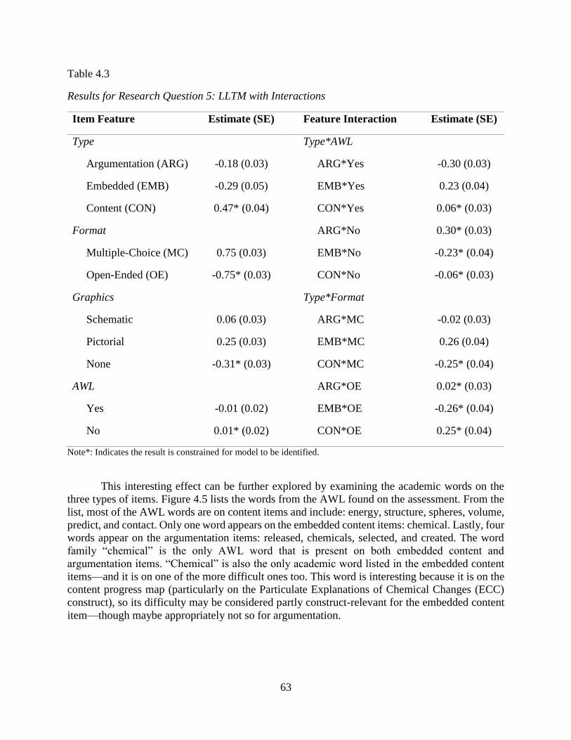
63

Table 4.3

Results for Research Question 5: LLTM with Interactions

Item Feature Estimate (SE) Feature Interaction Estimate (SE)

Type Type*AWL

Argumentation (ARG) -0.18 (0.03) ARG*Yes -0.30 (0.03)

Embedded (EMB) -0.29 (0.05) EMB*Yes 0.23 (0.04)

Content (CON) 0.47* (0.04) CON*Yes 0.06* (0.03)

Format ARG*No 0.30* (0.03)

Multiple-Choice (MC) 0.75 (0.03) EMB*No -0.23* (0.04)

Open-Ended (OE) -0.75* (0.03) CON*No -0.06* (0.03)

Graphics Type*Format

Schematic 0.06 (0.03) ARG*MC -0.02 (0.03)

Pictorial 0.25 (0.03) EMB*MC 0.26 (0.04)

None -0.31* (0.03) CON*MC -0.25* (0.04)

AWL ARG*OE 0.02* (0.03)

Yes -0.01 (0.02) EMB*OE -0.26* (0.04)

No 0.01* (0.02) CON*OE 0.25* (0.04)

Note*: Indicates the result is constrained for model to be identified.

This interesting effect can be further explored by examining the academic words on the

three types of items. Figure 4.5 lists the words from the AWL found on the assessment. From the

list, most of the AWL words are on content items and include: energy, structure, spheres, volume,

predict, and contact. Only one word appears on the embedded content items: chemical. Lastly, four

words appear on the argumentation items: released, chemicals, selected, and created. The word

family “chemical” is the only AWL word that is present on both embedded content and

argumentation items. “Chemical” is also the only academic word listed in the embedded content

items—and it is on one of the more difficult ones too. This word is interesting because it is on the

content progress map (particularly on the Particulate Explanations of Chemical Changes (ECC)

construct), so its difficulty may be considered partly construct-relevant for the embedded content

item—though maybe appropriately not so for argumentation.

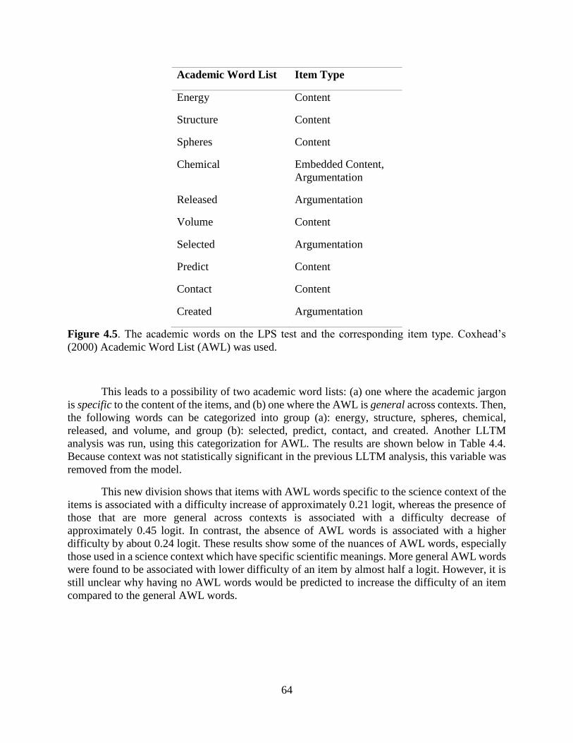
64

Academic Word List Item Type

Energy Content

Structure Content

Spheres Content

Chemical Embedded Content,

Argumentation

Released Argumentation

Volume Content

Selected Argumentation

Predict Content

Contact Content

Created Argumentation

Figure 4.5. The academic words on the LPS test and the corresponding item type. Coxhead’s

(2000) Academic Word List (AWL) was used.

This leads to a possibility of two academic word lists: (a) one where the academic jargon

is specific to the content of the items, and (b) one where the AWL is general across contexts. Then,

the following words can be categorized into group (a): energy, structure, spheres, chemical,

released, and volume, and group (b): selected, predict, contact, and created. Another LLTM

analysis was run, using this categorization for AWL. The results are shown below in Table 4.4.

Because context was not statistically significant in the previous LLTM analysis, this variable was

removed from the model.

This new division shows that items with AWL words specific to the science context of the

items is associated with a difficulty increase of approximately 0.21 logit, whereas the presence of

those that are more general across contexts is associated with a difficulty decrease of

approximately 0.45 logit. In contrast, the absence of AWL words is associated with a higher

difficulty by about 0.24 logit. These results show some of the nuances of AWL words, especially

those used in a science context which have specific scientific meanings. More general AWL words

were found to be associated with lower difficulty of an item by almost half a logit. However, it is

still unclear why having no AWL words would be predicted to increase the difficulty of an item

compared to the general AWL words.

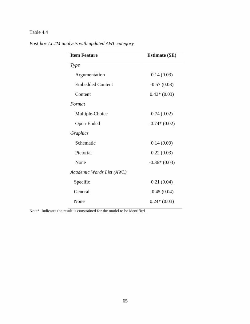
65

Table 4.4

Post-hoc LLTM analysis with updated AWL category

Item Feature Estimate (SE)

Type

Argumentation 0.14 (0.03)

Embedded Content -0.57 (0.03)

Content 0.43* (0.03)

Format

Multiple-Choice 0.74 (0.02)

Open-Ended -0.74* (0.02)

Graphics

Schematic 0.14 (0.03)

Pictorial 0.22 (0.03)

None -0.36* (0.03)

Academic Words List (AWL)

Specific 0.21 (0.04)

General -0.45 (0.04)

None 0.24* (0.03)

Note*: Indicates the result is constrained for the model to be identified.

66

4.3.4 Model Comparisons

Three models are compared below in Table 4.5. The unidimensional partial credit model

listed here is the same as from Chapter 2 (Equation 2.1). All LLTM models will be directly

compared to this partial credit model. The LLTM is the same as listed in Table 4.2. The LLTM

with interactions is the same as listed in Table 4.3.

Table 4.5

Model Comparisons: Partial Credit Model, LLTM, LLTM plus Interactions

Model # Parameters AIC BIC

Partial Credit Model 59 12797.52 12823.72

LLTM 12 17611.19 17616.52

LLTM plus Interactions 14 17489.98 17496.20

Likelihood ratio tests revealed that, as expected, the partial credit model had a statistically

significantly better fit than the LLTM (𝜒2 = 4907.67, 𝑑𝑓 = 47, 𝑝 < 0.001) and the LLTM with

interactions (𝜒2 = 4782.46, 𝑑𝑓 = 45, 𝑝 < 0.001). The significantly lower AIC and BIC values

also confirm these results. The partial credit model has a substantially better fit than any of the

LLTM models. However, it is often useful to examine the item features to see which play an

important role in explaining item difficulty, especially if there is a strong theory behind the

features. For instance, the LLTM confirms that there were no significant differences between the

contexts in terms of difficulty.

When comparing the two LLTM models, the LLTM with interactions has a statistically

better fit than the LLTM (𝜒2 = 125.21, 𝑑𝑓 = 2, 𝑝 < 0.001) and this is confirmed by comparing

the AIC and BIC values too.

Finally, Figures 4.6 and 4.7 provide a graphical view into how well the LLTM and LLTM

with interactions, respectively, match with the partial credit model results. The y-axis for these

two graphs is the step difficulties estimated from the partial credit model, while the x-axis is the

step difficulties estimated from the LLTMs. From both graphs, it appears that the two LLTMs tend

to underestimate the difficulties (i.e. most points are above the identity line). The correlations

between the partial credit model with the LLTM and the LLTM with interactions are the same,

and moderate at 𝑟 = 0.61. That is, the LLTM with interactions did not increase the correlation, as

one might have expected.

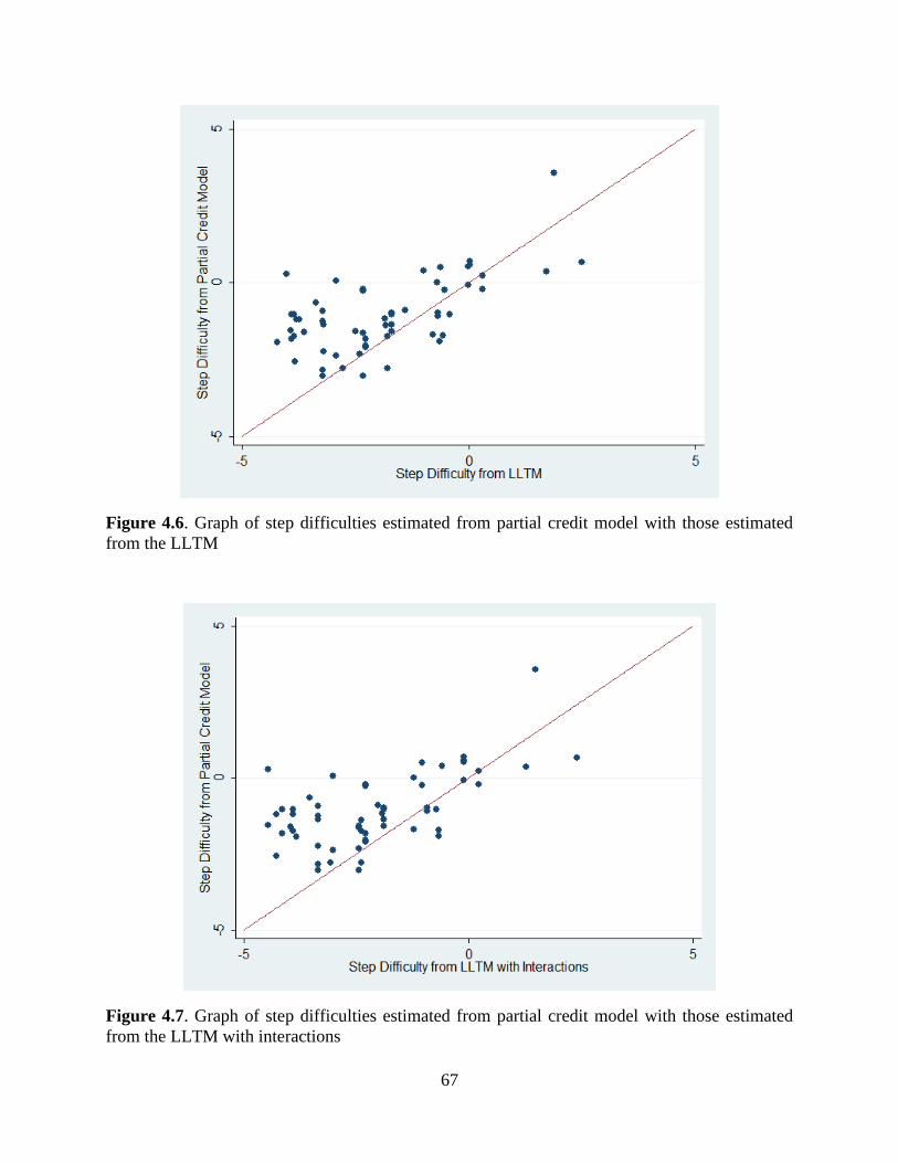
67

Figure 4.6. Graph of step difficulties estimated from partial credit model with those estimated

from the LLTM

Figure 4.7. Graph of step difficulties estimated from partial credit model with those estimated

from the LLTM with interactions

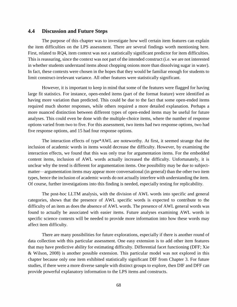
68

4.4 Discussion and Future Steps

The purpose of this chapter was to investigate how well certain item features can explain

the item difficulties on the LPS assessment. There are several findings worth mentioning here.

First, related to RQ4, item context was not a statistically significant predictor for item difficulties.

This is reassuring, since the context was not part of the intended construct (i.e. we are not interested

in whether students understand items about chopping onions more than dissolving sugar in water).

In fact, these contexts were chosen in the hopes that they would be familiar enough for students to

limit construct-irrelevant variance. All other features were statistically significant.

However, it is important to keep in mind that some of the features were flagged for having

large fit statistics. For instance, open-ended items (part of the format feature) were identified as

having more variation than predicted. This could be due to the fact that some open-ended items

required much shorter responses, while others required a more detailed explanation. Perhaps a

more nuanced distinction between different types of open-ended items may be useful for future

analyses. This could even be done with the multiple-choice items, where the number of response

options varied from two to five. For this assessment, two items had two response options, two had

five response options, and 15 had four response options.

The interaction effects of type*AWL are noteworthy. At first, it seemed strange that the

inclusion of academic words in items would decrease the difficulty. However, by examining the

interaction effects, we found that this was only true for argumentation items. For the embedded

content items, inclusion of AWL words actually increased the difficulty. Unfortunately, it is

unclear why the trend is different for argumentation items. One possibility may be due to subject-

matter—argumentation items may appear more conversational (in general) than the other two item

types, hence the inclusion of academic words do not actually interfere with understanding the item.

Of course, further investigations into this finding is needed, especially testing for replicability.

The post-hoc LLTM analysis, with the division of AWL words into specific and general

categories, shows that the presence of AWL specific words is expected to contribute to the

difficulty of an item as does the absence of AWL words. The presence of AWL general words was

found to actually be associated with easier items. Future analyses examining AWL words in

specific science contexts will be needed to provide more information into how these words may

affect item difficulty.

There are many possibilities for future explorations, especially if there is another round of

data collection with this particular assessment. One easy extension is to add other item features

that may have predictive ability for estimating difficulty. Differential facet functioning (DFF; Xie

& Wilson, 2008) is another possible extension. This particular model was not explored in this

chapter because only one item exhibited statistically significant DIF from Chapter 3. For future

studies, if there were a more diverse sample with distinct groups to explore, then DIF and DFF can

provide powerful explanatory information to the LPS items and constructs.

69

References

Abedi, J. (2008). Classification system for English language learners: Issues and

recommendations. Educational Measurement: Issues and Practice, 27(3), 17–31.

http://doi.org/10.1111/j.1745-3992.2008.00125.x

Adams, R. J. & Khoo, S. T. (1996). Quest. Melbourne, Australia: Australian Council for

Educational Research.

Adams, R. J., Wilson, M., & Wu, M. (1997). Multilevel item response models: An approach to

errors in variables regression. Journal of Educational and Behavioral Statistics, 22(1), 47–

76. http://doi.org/10.3102/10769986022001047

Adams, R. J., Wu, M., & Wilson, M. (2012). ConQuest 3.0 [computer program]. Hawthorn,

Australia: ACER.

Akaike, H. (1974). A new look at the statistical model identification. IEEE Transactions on

Automatic Control, 19(6), 716–723.

American Educational Research Association (AERA), American Psychological Association

(APA), National Council for Measurement in Education (NCME). (2014). Standards for

educational and psychological testing. Washington, DC: American Educational Research

Association.

Asterhan, C. S., Schwarz, B. B., & Gil, J. (2012). Small-group, computer-mediated argumentation

in middle-school classrooms: The effects of gender and different types of online teacher

guidance. British Journal of Educational Psychology, 82(3), 375–397.

Avenia-Tapper, B. & Llosa, L. (2015). Construct relevant or irrelevant? The role of linguistic

complexity in the assessment of English language learners’ science knowledge.

Educational Assessment, 20(2), 95–111. http://doi.org/10.1080/10627197.2015.1028622

Briggs, D. C. & Wilson, M. (2003). An introduction to multidimensional measurement using

Rasch models. Journal of Applied Measurement, 4(1), 87–100.

Brown, C. L. (2007). Supporting English language learners in content-reading. Reading

Improvement, 44(1), 32–39.

Bunch, G. C., Walqui, A., & Pearson, P. D. (2014). Complex text and new common standards in

the United States: Pedagogical implications for English learners. TESOL Quarterly, 48(3),

533–559. http://doi.org/10.1002/tesq.175

Catsambis, S. (1995). Gender, race, ethnicity, and science education in the middle grades. Journal

of Research in Science Teaching, 32(3), 243–257.

Cobb, T. (n.d.) Web Vocabprofile. Retrieved from http://www.lextutor.ca/vp/

70

Cohen, J. (1988). Statistical power analysis for the behavioral sciences (2nd ed.). Hillsdale, NJ:

Lawrence Erlbaum.

Coxhead, A. (2000). A new academic word list. TESOL Quarterly, 34(2), 213–238.

De Boeck, P. & Wilson, M. (2004). A framework for item response models. In P. De Boeck &

Wilson, M. (Eds.), Explanatory item response models: A generalized linear and nonlinear

approach (pp. 3-41). New York: Springer.

Embretson, S. E. (1983). Construct validity: Construct representation versus nomothetic span.

Psychological Bulletin, 93(1), 179–197. http://doi.org/10.1037/0033-2909.93.1.179

Fischer, G. H. (1973). The linear logistic test model as an instrument in educational research. Acta

Psychologica, 37(6), 359–374.

Fischer, G. H. & Ponocny, I. (1994). An extension of the partial credit model with an application

to the measurement of change. Psychometrika, 59(2), 177-192.

Flesch, R. (1951). How to test readability. New York: Harper & Brothers.

Ford, M. (2008). Disciplinary authority and accountability in scientific practice and learning.

Science Education, 92(3), 404–423. http://doi.org/10.1002/sce.20263

Haag, N., Roppelt, A. & Heppt, B. (2015). Effects of mathematics items’ language demands for

language minority students: Do they differ between grades? Learning and Individual

Differences, 42, 70–76. http://doi.org/10.1016/j.lindif.2015.08.010

Haladyna, T. M. & Downing, S. M. (2004). Construct-irrelevant variance in high-stakes testing.

Educational Measurement: Issues and Practice, 23(1), 17–27.

Hartig, J. & Höhler, J. (2009). Multidimensional IRT models for the assessment of competencies.

Studies in Educational Evaluation, 35(2-3), 57–63.

Hartig, J., Frey, A., Nold, G., & Klieme, E. (2011). An application of explanatory item response

modeling for model-based proficiency scaling. Educational and Psychological

Measurement. http://doi.org/10.1177/0013164411430707

Hohensinn, C. & Kubinger, K. D. (2011). Applying item response theory methods to examine the

impact of different response formats. Educational and Psychological Measurement, 71(4),

732–746. http://doi.org/10.1177/0013164410390032

Hyde, J. S. & Linn, M. C. (2006). Gender similarities in mathematics and science. Science,

314(5799), 599–600. http://doi.org/10.1126/science.1132154

Kincaid, J. P., Fishburne, R. P., Rogers, R. L., & Chissom, B. S. (1975). Derivation of new

readability formulas (Automated Readability Index, Fog Count, and Flesch Reading Ease

formulas) for Navy enlisted personnel (Research Branch Report No. 8-75). Millington, TN:

Naval Technical Training.

Klare, G. R. (1984). Readability. In P.D. Pearson (Ed.), Handbook of reading research (pp. 681-

744). New York: Longman, Inc.

71

Kubinger, K. D. (2008). On the revival of the Rasch model-based LLTM: From constructing tests

using item generating rules to measuring item administration effects. Psychology Science,

50(3), 311–327.

Linacre, J. M. (1989). Multi-facet Rasch measurement. Chicago: MESA Press.

Liu, O. L., Wilson, M., & Paek, I. (2008). A multidimensional Rasch analysis of gender differences

in PISA mathematics. Journal of Applied Measurement, 9(1), 2–18.

Martiniello, M. (2009). Linguistic complexity, schematic representations, and differential item

functioning for English language learners in math tests. Educational Assessment, 14(3-4),

160–179. doi:10.1080/10627190903422906

Masters, G. N. (1982). A Rasch model for partial credit scoring. Psychometrika, 47(2), 149–174.

Meulders, M. & Xie, Y. (2004). Person-by-item predictors. In P. De Boeck & M. Wilson (Eds.),

Explanatory item response models: A generalized linear and nonlinear approach (pp. 213–

240). New York: Springer.

Millsap, R. E. & Everson, H. T. (1993). Methodology review: Statistical approaches for assessing

measurement bias. Applied Psychological Measurement, 17(4), 297–334.

doi:10.1177/014662169301700401

National Research Council. (2011). A framework for K-12 science education practices,

crosscutting concepts, and core ideas. Washington, D.C.: National Academies Press.

Retrieved from http://www.nap.edu/catalog.php?record_id=13165

Naylor, S., Keogh, B., & Downing, B. (2007). Argumentation and primary science. Research in

Science Education, 37(1), 17–39. http://doi.org/10.1007/s11165-005-9002-5

NGSS Lead States. (2013). Next Generation Science Standards: For States, By States.

Washington, D.C: The National Academies Press.

Osborne, J., Henderson, J. B., MacPherson, A., & Szu, E. (2013a, May). Building a learning

progression for argumentation in science education. Presentation at the American

Educational Research Association (AERA) conference, San Francisco.

Osborne, J., Henderson, J. B., Szu, E., MacPherson, A., & Yao, S.-Y. (2013b, May). Validating

and assessing a new progress map for student argumentation in science. Presentation at

the American Educational Research Association (AERA) conference, San Francisco.

Osterlind, S. J. & Everson, H. T. (2009). Differential item functioning (2nd ed.). Thousand Oaks,

Calif: SAGE.

Paek, I. (2002). Investigations of differential item functioning: Comparisons among approaches

and extension to a multidimensional context (Unpublished doctoral dissertation).

University of California, Berkeley.

R Core Team (2015). R: A language and environment for statistical computing. R Foundation for

Statistical Computing, Vienna, Austria. URL: http://www.R-project.org/

72

Rabe-Hesketh, S. & Skrondal, A. (2008). Multilevel and longitudinal modeling using Stata (2nd

ed.). College Station, TX: Stata Press.

Schwartz, R. & Ayers, E. (2011). Delta dimensional alignment: Comparing performances across

dimensions of the learning progression for Assessing Data Modeling and Statistical

Reasoning. Unpublished manuscript, School of Education, University of California,

Berkeley.

Schwarz, G. (1978). Estimating the dimension of a model. The Annals of Statistics, 6(2), 461–464.

StataCorp. (2009). Stata Statistical Software: Release 11. College Station, TX: StataCorp LP.

Stevens, R. A., Butler, F. A., & Castellon-Wellington, M. (2001). Academic language and content

assessment: Measuring the progress of English language learners (ELLs) (Technical No.

552). Los Angeles, CA: CRESST/ University of California, Los Angeles.

Torres Irribarra, D. & Freund, R. (2016). WrightMap: IRT item-person map with ConQuest

integration. Available at http://github.com/david-ti/wrightmap

Toulmin, S. (1958). The uses of argument. Cambridge: Cambridge University Press.

Van den Noortgate, W. & Paek, I. (2004). Person regression models. In P. De Boeck & M. Wilson

(Eds.), Explanatory item response models: A generalized linear and nonlinear approach

(pp. 167–187). New York: Springer.

Walker, C. M. & Beretvas, S. N. (2003). Comparing multidimensional and unidimensional

proficiency classifications: Multidimensional IRT as a diagnostic aid. Journal of

Educational Measurement, 40(3), 255–275. doi:10.1111/j.1745-3984.2003.tb01107.x

Walker, C. M., Zhang, B., & Surber, J. (2008). Using a multidimensional differential item

functioning framework to determine if reading ability affects student performance in

mathematics. Applied Measurement in Education, 21(2), 162–181.

Wang, W.-C., & Wilson, M. (2005). The Rasch testlet model. Applied Psychological

Measurement, 29(2), 126–149. doi:10.1177/0146621604271053

Wang, W.-C., Wilson, M., & Adams, R. J. (1997). Rasch models for multidimensionality between

items and within items. In M. Wilson & G. Engelhard (Eds.), Objective measurement:

Theory into practice (Vol. IV). Norwood, NJ: Ablex.

Weinburgh, M. (1995). Gender differences in student attitudes toward science: A meta-analysis of

the literature from 1970 to 1991. Journal of Research in Science Teaching, 32(4), 387–

398. http://doi.org/10.1002/tea.3660320407

Wilson, C. D., Taylor, J. A., Kowalski, S. M., & Carlson, J. (2009). The relative effects and equity

of inquiry-based and commonplace science teaching on students’ knowledge, reasoning,

and argumentation. Journal of Research in Science Teaching, 47(3), 276-301.

Wilson, M. (2005). Constructing measures: An item response modeling approach. Mahwah, N.J:

Lawrence Erlbaum Associates.

73

Wilson, M., Black, P., & Morell, L. (2013, May). A learning progression approach to

understanding students? Conceptions of the structure of matter. Presentation at the

American Educational Research Association (AERA) conference, San Francisco.

Wilson, M. & Sloane, K. (2000). From principles to practice: An embedded assessment system.

Applied Measurement in Education, 13(2), 181–208.

Wolf, M. K. & Leon, S. (2009). An investigation of the language demands in content assessments

for English language learners. Educational Assessment, 14(3), 139–159.

doi:10.1080/10627190903425883

Wu, M. & Adams, R. (2006). Modelling mathematics problem solving item responses using a

multidimensional IRT model. Mathematics Education Research Journal, 18(2), 93–113.

Wu, M., Adams, R., Wilson, M., & Haldane, S. A. (2007). ConQuest (Version 2.0) Manual.

Hawthorn, Australia: ACER.

Xie, Y., & Wilson, M. (2008). Investigating DIF and extensions using an LLTM approach and

also an individual differences approach: An international testing context. Psychology

Science Quarterly, 50(3), 403–416.

Yao, S.-Y. (2013). Investigating the validity of a scientific argumentation assessment using

psychometric methods (Unpublished doctoral dissertation). University of California,

Berkeley.

Yao, S.-Y., Wilson, M., Henderson, J. B., & Osborne, J. (2105). Investigating the function of

content and argumentation items in a science test: A multidimensional approach. Journal

of Applied Measurement, 16(2), 171-192.