Time Warping Hidden Markov Models Lecture 2, Thursday April 3, 2003.
32
Time Warping Hidden Markov Models Lecture 2, Thursday April 3, 2003
-
date post
21-Dec-2015 -
Category
Documents
-
view
214 -
download
0
Transcript of Time Warping Hidden Markov Models Lecture 2, Thursday April 3, 2003.

Time WarpingHidden Markov Models
Lecture 2, Thursday April 3, 2003

Review of Last Lecture
Lecture 2, Thursday April 3, 2003
Lecture 4, Thursday April 10, 2003
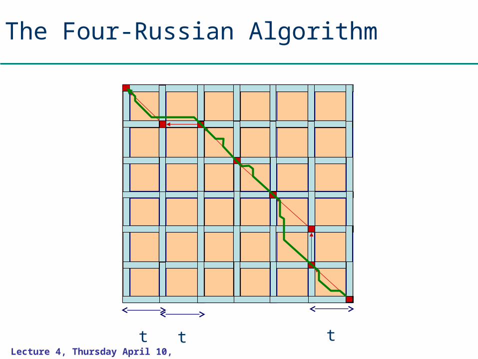
The Four-Russian Algorithm
t t t
Lecture 4, Thursday April 10, 2003
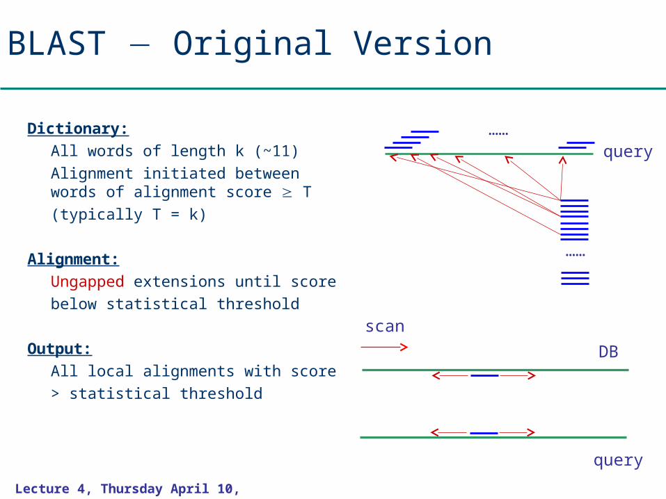
BLAST Original Version
Dictionary:All words of length k (~11)Alignment initiated between words of alignment score T
(typically T = k)
Alignment:Ungapped extensions until score
below statistical threshold
Output:All local alignments with score
> statistical threshold
……
……
query
DB
query
scan
Lecture 4, Thursday April 10, 2003
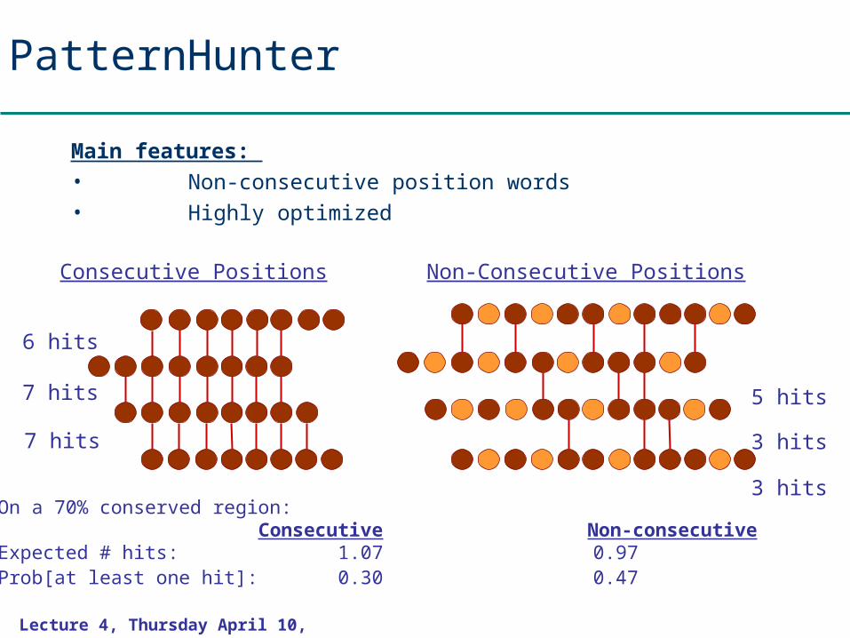
PatternHunter
Main features: • Non-consecutive position words• Highly optimized
5 hits
3 hits
3 hits
7 hits
7 hits
Consecutive Positions Non-Consecutive Positions
6 hits
On a 70% conserved region: Consecutive Non-consecutive
Expected # hits: 1.07 0.97Prob[at least one hit]: 0.30 0.47

Lecture 4, Thursday April 10, 2003
Today
• Time Warping
• Hidden Markov models
Lecture 4, Thursday April 10, 2003
Time WarpingTime Warping
Lecture 4, Thursday April 10, 2003
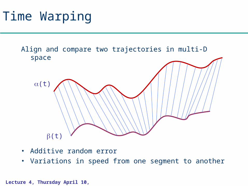
Time Warping
Align and compare two trajectories in multi-D space
(t)
(t)
• Additive random error• Variations in speed from one segment to another
Lecture 4, Thursday April 10, 2003
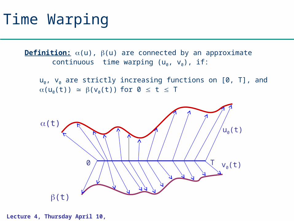
Time Warping
Definition: (u), (u) are connected by an approximate continuous time warping (u0, v0), if:
u0, v0 are strictly increasing functions on [0, T], and (u0(t)) (v0(t)) for 0 t T
(t)
(t)
0 T
u0(t)
v0(t)
Lecture 4, Thursday April 10, 2003
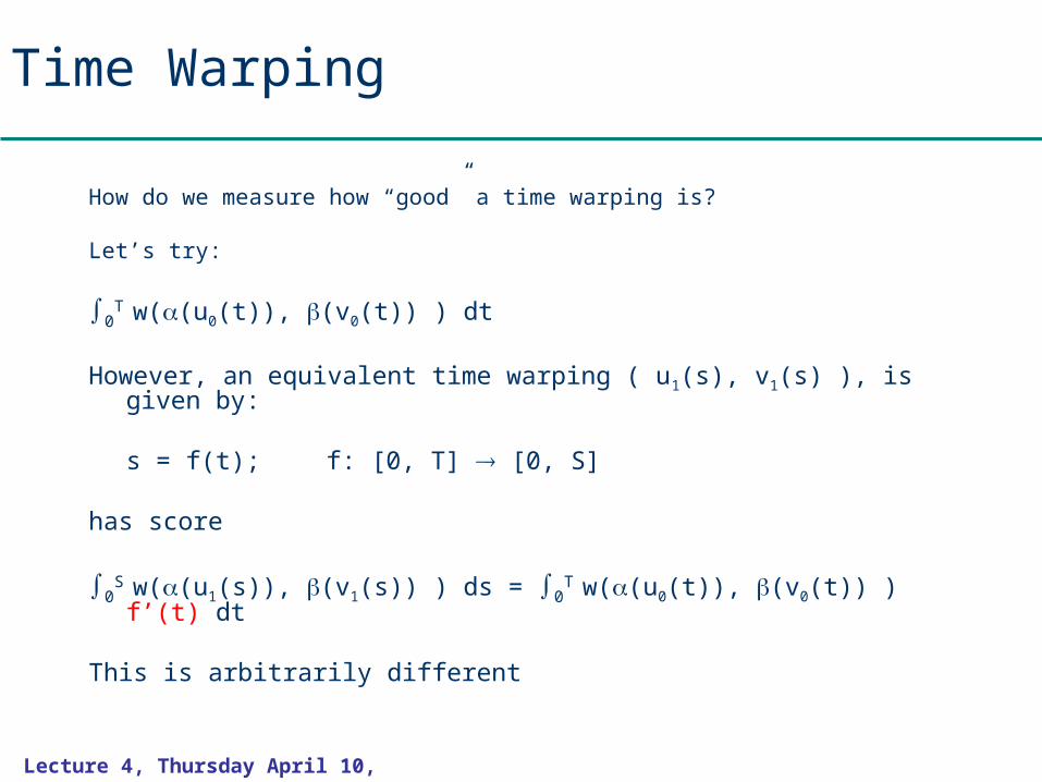
Time Warping
How do we measure how “good” a time warping is?
Let’s try:
0T w((u0(t)), (v0(t)) ) dt
However, an equivalent time warping ( u1(s), v1(s) ), is given by:
s = f(t); f: [0, T] [0, S]
has score
0S w((u1(s)), (v1(s)) ) ds = 0
T w((u0(t)), (v0(t)) ) f’(t) dt
This is arbitrarily different
Lecture 4, Thursday April 10, 2003
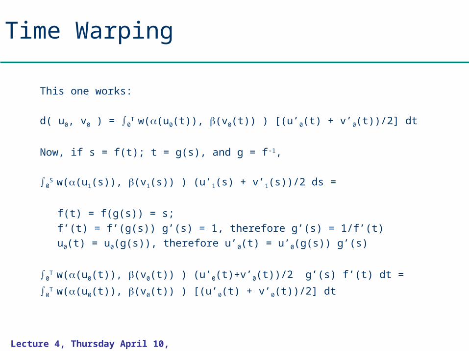
Time Warping
This one works:
d( u0, v0 ) = 0T w((u0(t)), (v0(t)) ) [(u’0(t) + v’0(t))/2] dt
Now, if s = f(t); t = g(s), and g = f-1,
0S w((u1(s)), (v1(s)) ) (u’1(s) + v’1(s))/2 ds =
f(t) = f(g(s)) = s;f’(t) = f’(g(s)) g’(s) = 1, therefore g’(s) = 1/f’(t)u0(t) = u0(g(s)), therefore u’0(t) = u’0(g(s)) g’(s)
0T w((u0(t)), (v0(t)) ) (u’0(t)+v’0(t))/2 g’(s) f’(t) dt =
0T w((u0(t)), (v0(t)) ) [(u’0(t) + v’0(t))/2] dt
Lecture 4, Thursday April 10, 2003
Time Warping
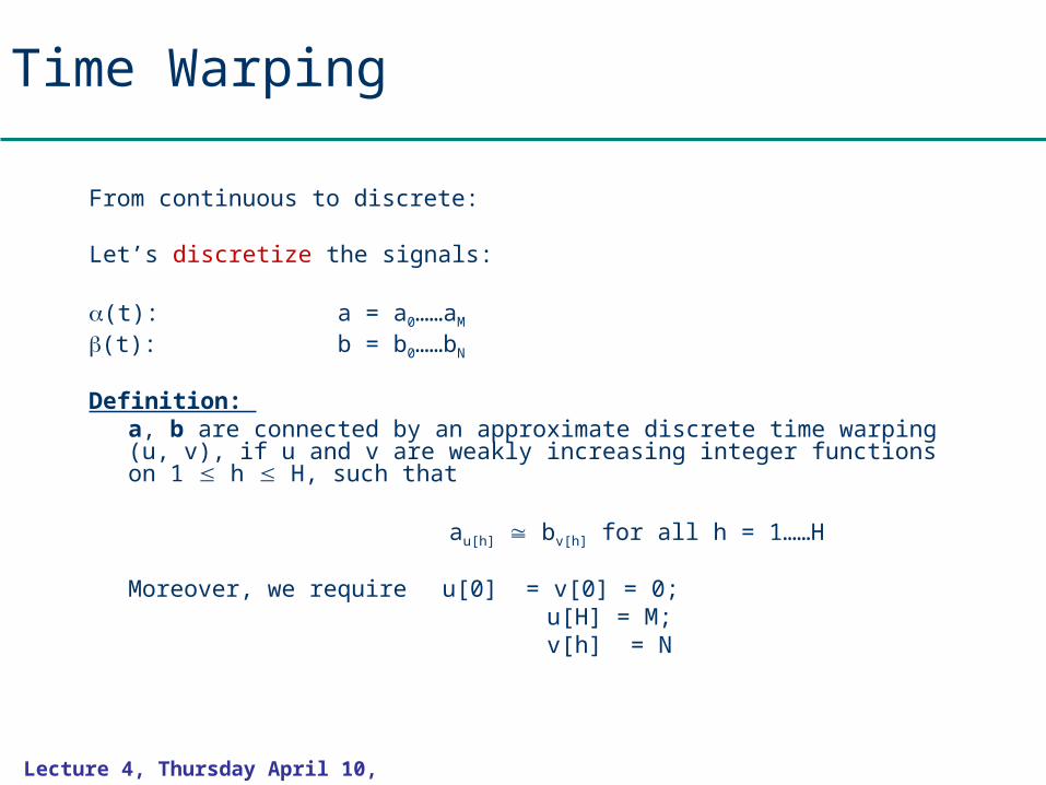
From continuous to discrete:
Let’s discretize the signals:
(t): a = a0……aM
(t): b = b0……bN
Definition: a, b are connected by an approximate discrete time warping (u, v), if u and v are weakly increasing integer functions on 1 h H, such that
au[h] bv[h] for all h = 1……H
Moreover, we require u[0] = v[0] = 0; u[H] = M; v[h] = N
Lecture 4, Thursday April 10, 2003
Time Warping
v
u0
0
1 2
12
M
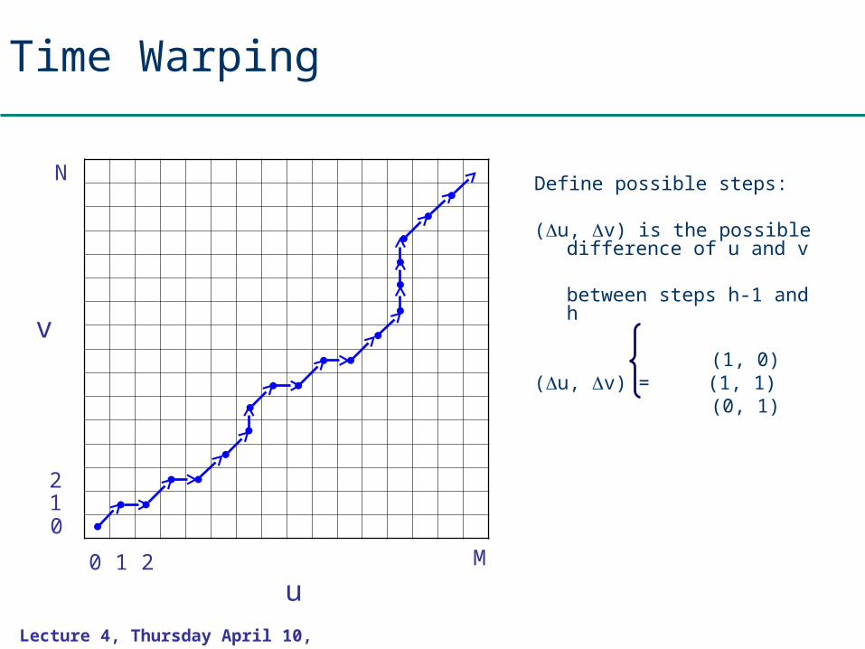
N Define possible steps:
(u, v) is the possible difference of u and v
between steps h-1 and h
(1, 0)(u, v) = (1, 1)
(0, 1)
Lecture 4, Thursday April 10, 2003
Time Warping
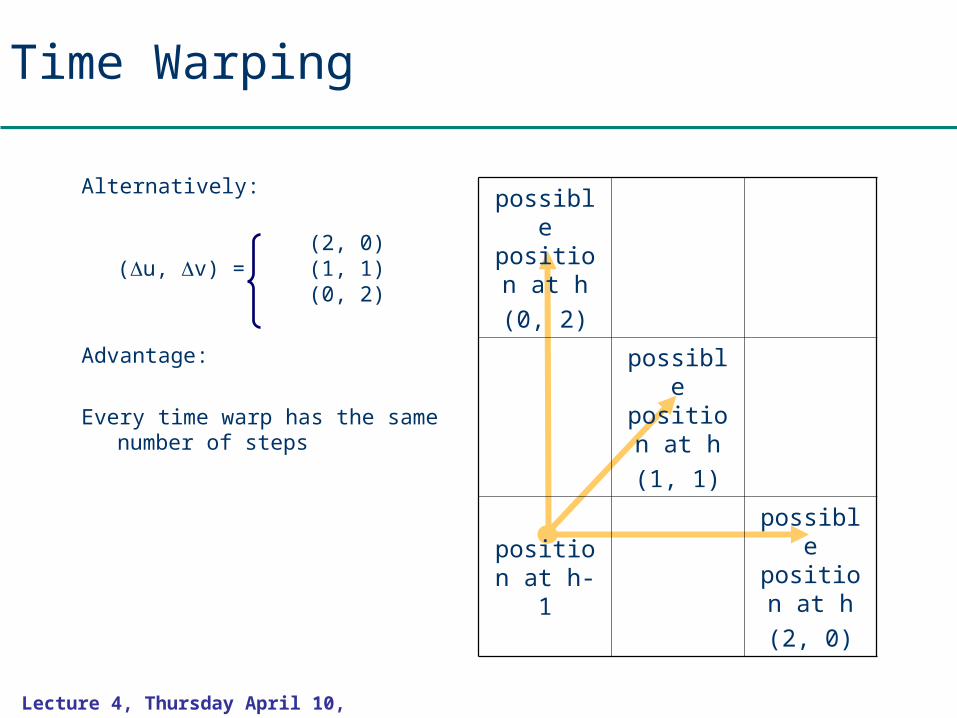
Alternatively:
(2, 0)(u, v) = (1, 1)
(0, 2)
Advantage:
Every time warp has the same number of steps
possible position
at h(0, 2)
possible position
at h(1, 1)
position at h-1
possible position
at h(2, 0)
Lecture 4, Thursday April 10, 2003
Time Warping
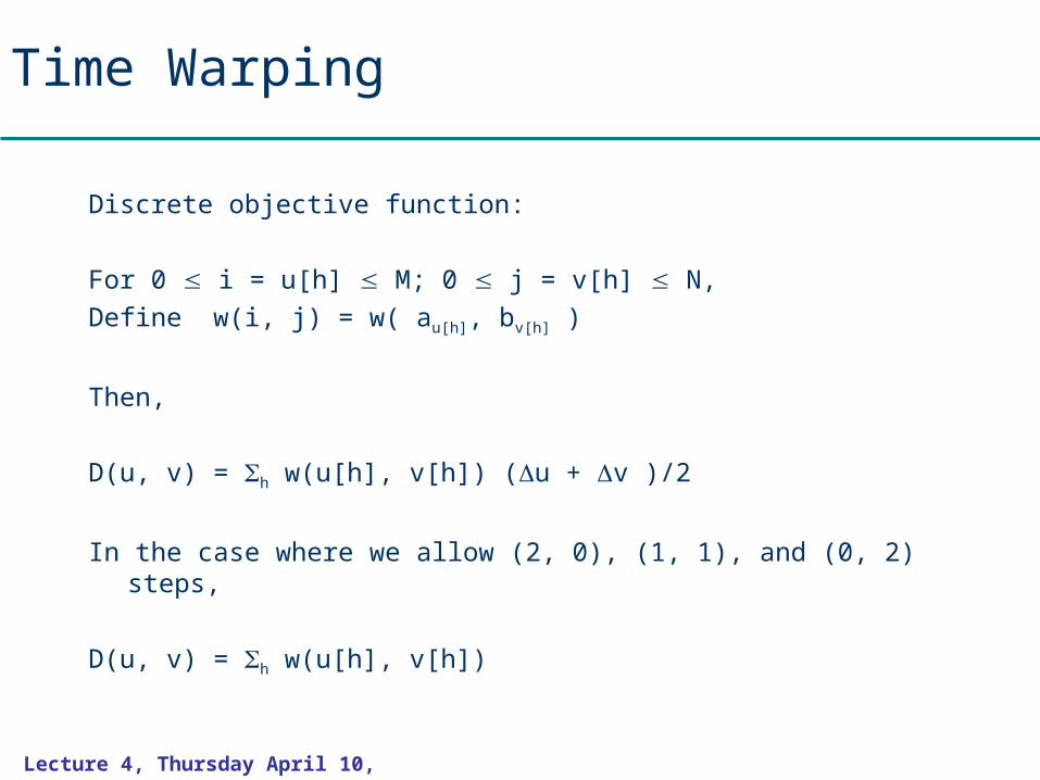
Discrete objective function:
For 0 i = u[h] M; 0 j = v[h] N,Define w(i, j) = w( au[h], bv[h] )
Then,
D(u, v) = h w(u[h], v[h]) (u + v )/2
In the case where we allow (2, 0), (1, 1), and (0, 2) steps,
D(u, v) = h w(u[h], v[h])
Lecture 4, Thursday April 10, 2003
Time Warping
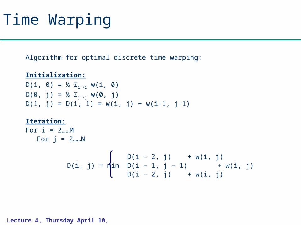
Algorithm for optimal discrete time warping:
Initialization: D(i, 0) = ½ i’<i w(i, 0)
D(0, j) = ½ j’<j w(0, j)D(1, j) = D(i, 1) = w(i, j) + w(i-1, j-1)
Iteration:For i = 2……M
For j = 2……N
D(i – 2, j) + w(i, j)D(i, j) = min D(i – 1, j – 1) + w(i, j)
D(i – 2, j) + w(i, j)
Hidden Markov Models1
2
K
…
1
2
K
…
1
2
K
…
…
…
…
1
2
K
…
x1 x2 x3 xK
2
1
K
2

Lecture 4, Thursday April 10, 2003
Outline for our next topic
• Hidden Markov models – the theory
• Probabilistic interpretation of alignments using HMMs
Later in the course:
• Applications of HMMs to biological sequence modeling and discovery of features such as genes
Lecture 4, Thursday April 10, 2003
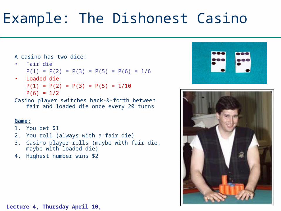
Example: The Dishonest Casino
A casino has two dice:• Fair die
P(1) = P(2) = P(3) = P(5) = P(6) = 1/6• Loaded die
P(1) = P(2) = P(3) = P(5) = 1/10P(6) = 1/2
Casino player switches back-&-forth between fair and loaded die once every 20 turns
Game:1. You bet $12. You roll (always with a fair die)3. Casino player rolls (maybe with fair die, maybe
with loaded die)4. Highest number wins $2
Lecture 4, Thursday April 10, 2003
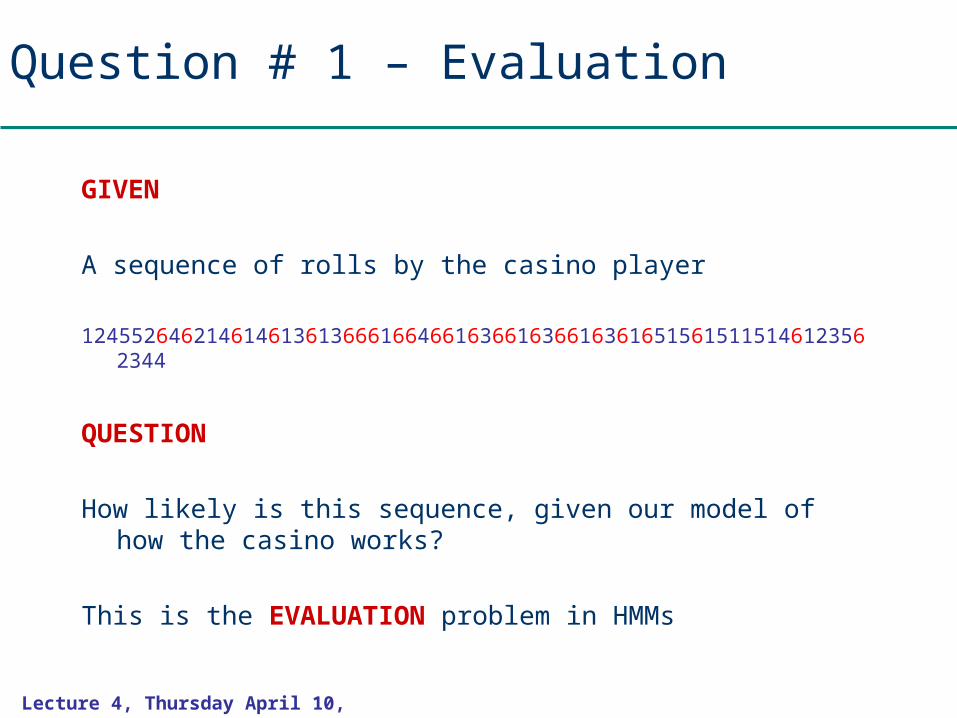
Question # 1 – Evaluation
GIVEN
A sequence of rolls by the casino player
1245526462146146136136661664661636616366163616515615115146123562344
QUESTION
How likely is this sequence, given our model of how the casino works?
This is the EVALUATION problem in HMMs
Lecture 4, Thursday April 10, 2003
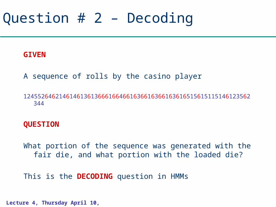
Question # 2 – Decoding
GIVEN
A sequence of rolls by the casino player
1245526462146146136136661664661636616366163616515615115146123562344
QUESTION
What portion of the sequence was generated with the fair die, and what portion with the loaded die?
This is the DECODING question in HMMs
Lecture 4, Thursday April 10, 2003
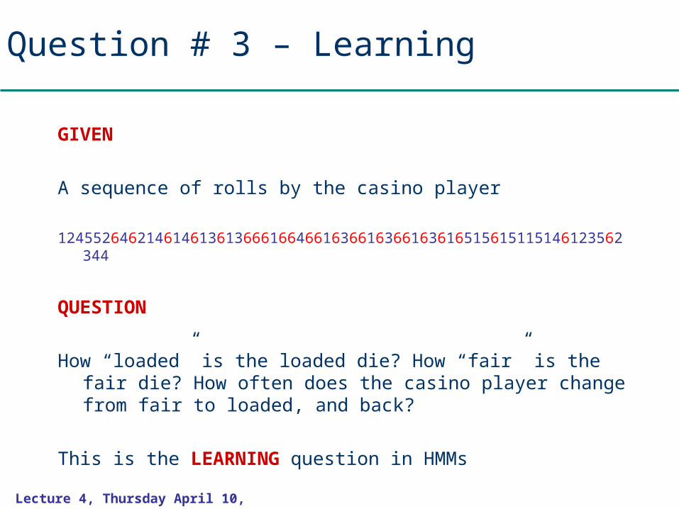
Question # 3 – Learning
GIVEN
A sequence of rolls by the casino player
1245526462146146136136661664661636616366163616515615115146123562344
QUESTION
How “loaded” is the loaded die? How “fair” is the fair die? How often does the casino player change from fair to loaded, and back?
This is the LEARNING question in HMMs
Lecture 4, Thursday April 10, 2003
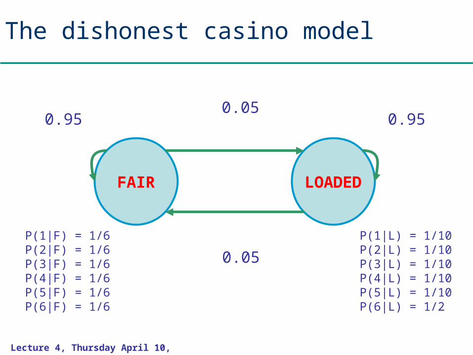
The dishonest casino model
FAIR LOADED
0.05
0.05
0.950.95
P(1|F) = 1/6P(2|F) = 1/6P(3|F) = 1/6P(4|F) = 1/6P(5|F) = 1/6P(6|F) = 1/6
P(1|L) = 1/10P(2|L) = 1/10P(3|L) = 1/10P(4|L) = 1/10P(5|L) = 1/10P(6|L) = 1/2
Lecture 4, Thursday April 10, 2003
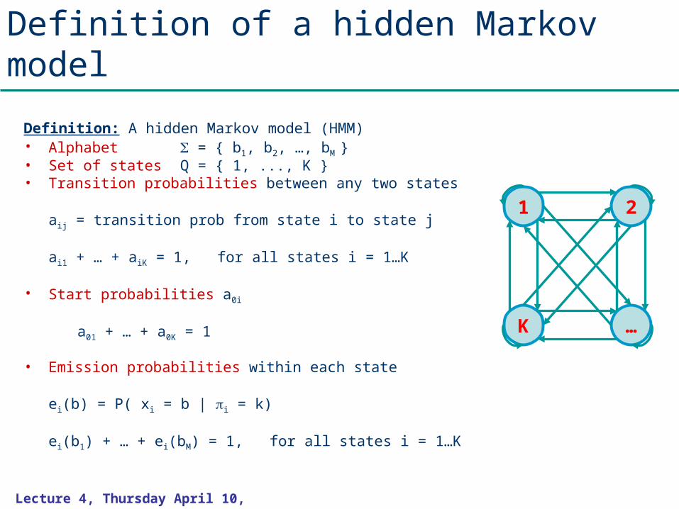
Definition of a hidden Markov model
Definition: A hidden Markov model (HMM)• Alphabet = { b1, b2, …, bM }• Set of states Q = { 1, ..., K }• Transition probabilities between any two states
aij = transition prob from state i to state j
ai1 + … + aiK = 1, for all states i = 1…K
• Start probabilities a0i
a01 + … + a0K = 1
• Emission probabilities within each state
ei(b) = P( xi = b | i = k)
ei(b1) + … + ei(bM) = 1, for all states i = 1…K
K
1
…
2
Lecture 4, Thursday April 10, 2003
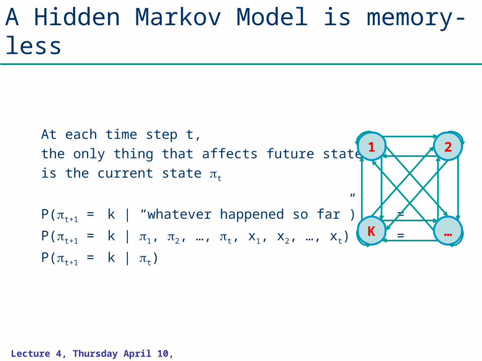
A Hidden Markov Model is memory-less
At each time step t, the only thing that affects future states is the current state t
P(t+1 = k | “whatever happened so far”) =
P(t+1 = k | 1, 2, …, t, x1, x2, …, xt) =
P(t+1 = k | t)
K
1
…
2
Lecture 4, Thursday April 10, 2003
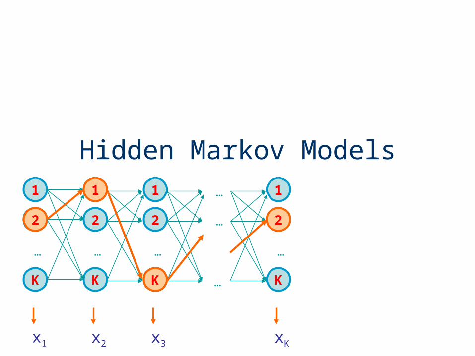
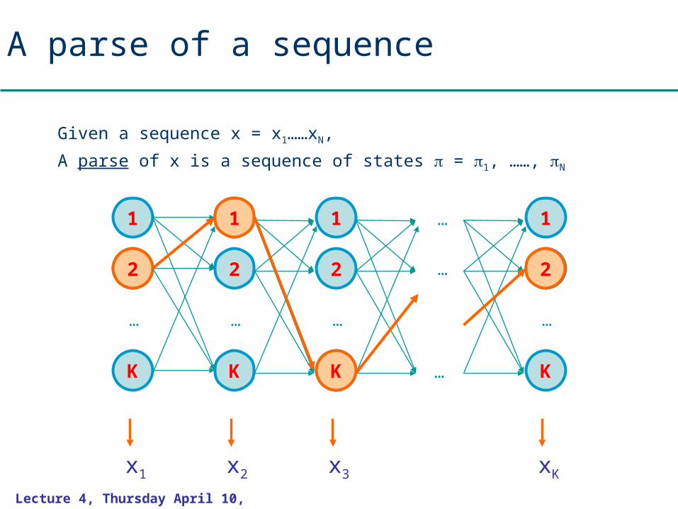
A parse of a sequence
Given a sequence x = x1……xN,
A parse of x is a sequence of states = 1, ……, N
1
2
K
…
1
2
K
…
1
2
K
…
…
…
…
1
2
K
…
x1 x2 x3 xK
2
1
K
2
Lecture 4, Thursday April 10, 2003
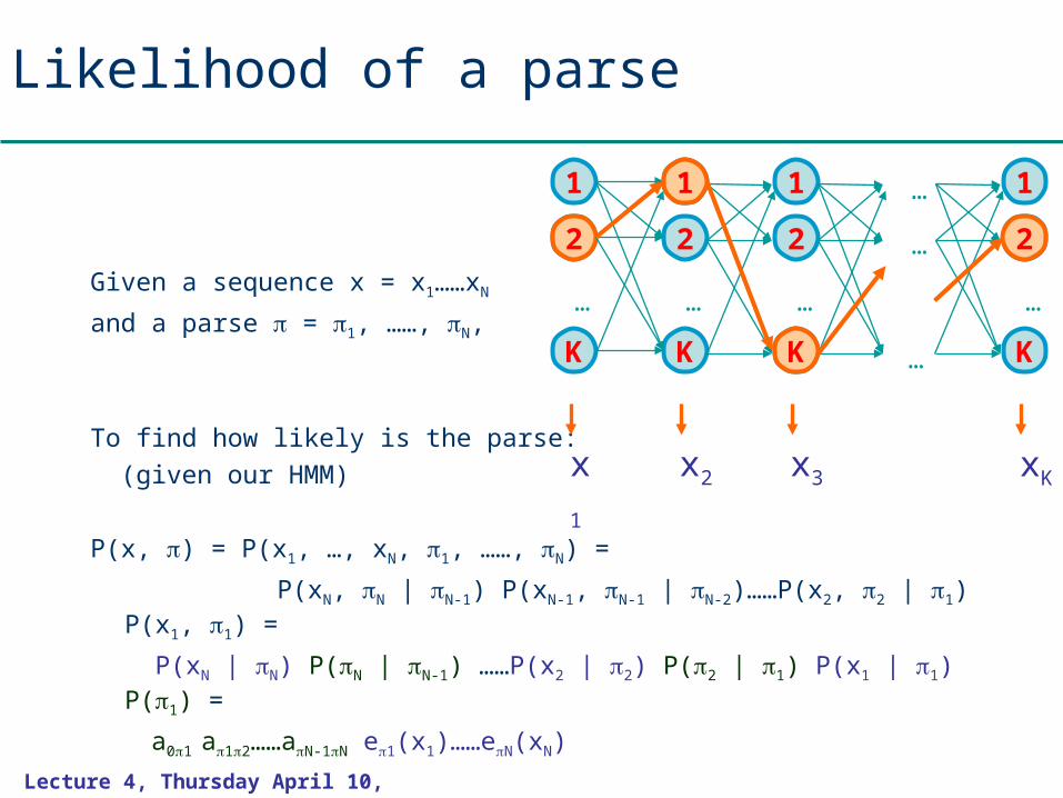
Likelihood of a parse
Given a sequence x = x1……xN
and a parse = 1, ……, N,
To find how likely is the parse: (given our HMM)
P(x, ) = P(x1, …, xN, 1, ……, N) =
P(xN, N | N-1) P(xN-1, N-1 | N-2)……P(x2, 2 | 1) P(x1, 1) =
P(xN | N) P(N | N-1) ……P(x2 | 2) P(2 | 1) P(x1 | 1) P(1) =
a01 a12……aN-1N e1(x1)……eN(xN)
1
2
K
…
1
2
K
…
1
2
K
…
…
…
…
1
2
K
…
x1
x2 x3 xK
2
1
K
2
Lecture 4, Thursday April 10, 2003
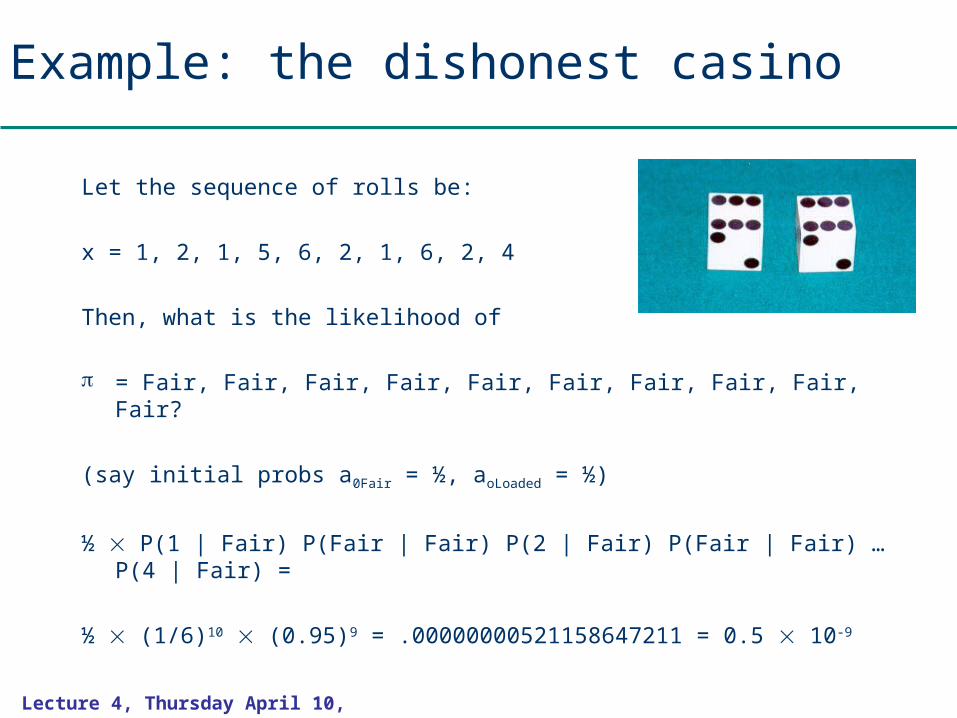
Example: the dishonest casino
Let the sequence of rolls be:
x = 1, 2, 1, 5, 6, 2, 1, 6, 2, 4
Then, what is the likelihood of
= Fair, Fair, Fair, Fair, Fair, Fair, Fair, Fair, Fair, Fair?
(say initial probs a0Fair = ½, aoLoaded = ½)
½ P(1 | Fair) P(Fair | Fair) P(2 | Fair) P(Fair | Fair) … P(4 | Fair) =
½ (1/6)10 (0.95)9 = .00000000521158647211 = 0.5 10-9

Lecture 4, Thursday April 10, 2003
Example: the dishonest casino
So, the likelihood the die is fair in all this runis just 0.521 10-9
OK, but what is the likelihood of
= Loaded, Loaded, Loaded, Loaded, Loaded, Loaded, Loaded, Loaded, Loaded, Loaded?
½ P(1 | Loaded) P(Loaded, Loaded) … P(4 | Loaded) =
½ (1/10)8 (1/2)2 (0.95)9 = .00000000078781176215 = 7.9 10-10
Therefore, it is after all 6.59 times more likely that the die is fair all the way, than that it is loaded all the way.
Lecture 4, Thursday April 10, 2003
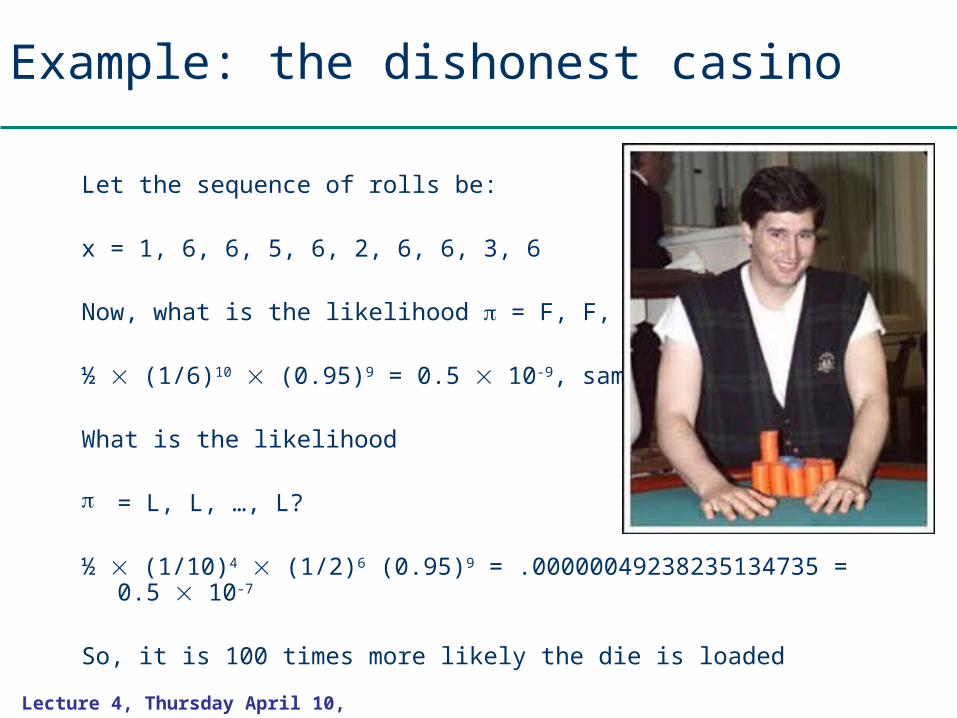
Example: the dishonest casino
Let the sequence of rolls be:
x = 1, 6, 6, 5, 6, 2, 6, 6, 3, 6
Now, what is the likelihood = F, F, …, F?
½ (1/6)10 (0.95)9 = 0.5 10-9, same as before
What is the likelihood
= L, L, …, L?
½ (1/10)4 (1/2)6 (0.95)9 = .00000049238235134735 = 0.5 10-
7
So, it is 100 times more likely the die is loaded
Lecture 4, Thursday April 10, 2003
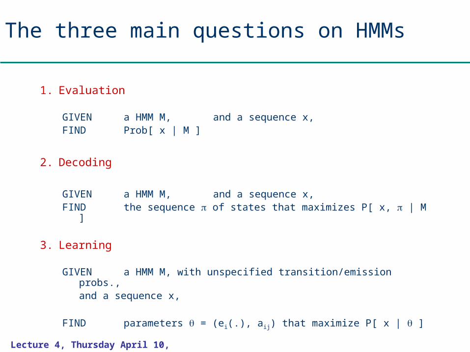
The three main questions on HMMs
1. Evaluation
GIVEN a HMM M, and a sequence x,FIND Prob[ x | M ]
2. Decoding
GIVEN a HMM M, and a sequence x,FIND the sequence of states that maximizes P[ x, | M ]
3. Learning
GIVEN a HMM M, with unspecified transition/emission probs.,and a sequence x,
FIND parameters = (ei(.), aij) that maximize P[ x | ]
Lecture 4, Thursday April 10, 2003
Let’s not be confused by notation
P[ x | M ]: The probability that sequence x was generated by the model
The model is: architecture (#states, etc) + parameters = aij, ei(.)
So, P[ x | ], and P[ x ] are the same, when the architecture, and the entire model, respectively, are implied
Similarly, P[ x, | M ] and P[ x, ] are the same
In the LEARNING problem we always write P[ x | ] to emphasize that we are seeking the that maximizes P[ x | ]