Time-Varying Structural Vector Autoregressions and ... · distribution of the model coe cients by...

This paper presents preliminary findings and is being distributed to economists

and other interested readers solely to stimulate discussion and elicit comments.

The views expressed in this paper are those of the authors and do not necessarily

reflect the position of the Federal Reserve Bank of New York or the Federal

Reserve System. Any errors or omissions are the responsibility of the authors.

Federal Reserve Bank of New York

Staff Reports

Time-Varying Structural Vector

Autoregressions and Monetary Policy:

A Corrigendum

Marco Del Negro

Giorgio Primiceri

Staff Report No. 619

May 2013

Revised October 2014

Time-Varying Structural Vector Autoregressions and Monetary Policy:

A Corrigendum Marco Del Negro and Giorgio Primiceri

Federal Reserve Bank of New York Staff Reports, no. 619

May 2013; revised October 2014

JEL classification: C11, C15

Abstract

This note corrects a mistake in the estimation algorithm of the time-varying structural vector

autoregression model of Primiceri (2005) and shows how to correctly apply the procedure of

Kim, Shephard, and Chib (1998) to the estimation of VAR, DSGE, factor, and unobserved

components models with stochastic volatility. Relative to Primiceri (2005), the main difference in

the new algorithm is the ordering of the various Markov Chain Monte Carlo steps, with each

individual step remaining the same.

Key words: Bayesian methods, time-varying volatility

_________________

Del Negro: Federal Reserve Bank of New York (e-mail: [email protected]). Primiceri:

Northwestern University (e-mail: [email protected]). The views expressed in this

paper are those of the authors and do not necessarily reflect the position of the Federal Reserve

Bank of New York or the Federal Reserve System.

Time Varying Structural Vector Autoregressions: A Corrigendum 1

1 The Model in Short

This note is a corrigendum of Primiceri (2005), but its lesson applies more broadly to several

empirical macro models with stochastic volatility that are estimated using the approach of

Kim, Shephard, and Chib (1998, KSC hereafter). Consider the time-varying VAR model of

Primiceri (2005)

yt = ct +B1,tyt−1 + ...+Bk,tyt−k + A−1t Σtεt, (1)

where yt is an n × 1 vector of observed endogenous variables; ct is a vector of time-varying

intercepts; Bi,t, i = 1, ..., k, are matrices of time-varying coefficients; At is a lower triangular

matrix with ones on the main diagonal and time-varying coefficients below it; Σt is a diagonal

matrix of time-varying standard deviations; εt is an n×1 vector of unobservable shocks with

variance equal to the identity matrix. All the time-varying coefficients evolve as random

walks, except for the diagonal elements of Σt, which behave as geometric random walks.

All the innovations in the model (shocks to coefficients, log-volatilities and εt) are jointly

normally distributed, with mean equal to zero and covariance matrix equal to V . The matrix

V is block diagonal, with blocks corresponding to the time-varying elements of the B’s, A,

Σ and ε. The block structure of the matrix V is described in detail in Primiceri (2005).

2 The Original Algorithm of Primiceri (2005) and Why

It is Wrong

The unknown objects of the model are the history of the volatilities (ΣT ), the history of

the coefficients (BT and AT ), and the covariance matrix of the innovations (V ). To simplify

the notation, define θ ≡[BT , AT , V

]. Primiceri (2005) proposed to simulate the posterior

distribution of the model coefficients by Gibbs sampling, drawing the history of volatilities

with the multi-move algorithm of KSC.

The difficulty with drawing ΣT is that they enter the model multiplicatively. For given θ,

however, simple algebraic manipulations of (1) yield a linear system in the log volatilities. A

consequence of applying these transformations is that they also convert εt into log ε2t , which


is a vector of logχ2 (1) random variables. The method of KSC relies on approximating

each element of log ε2t with a mixture of normals. Conditioning on the mixture indicators

makes it possible to use standard Gaussian state-space methods to conduct inference on

the volatilities. As a consequence, the Gibbs sampler is augmented to include the mixture

indicators sT ≡ {st}Tt=1 that select the component of the mixture for each variable at each

date.

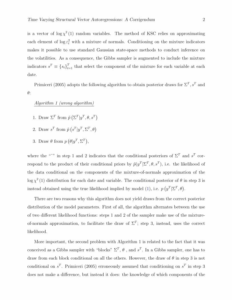
Primiceri (2005) adopts the following algorithm to obtain posterior draws for ΣT , sT and

θ:

Algorithm 1 (wrong algorithm)

1. Draw ΣT from p(ΣT |yT , θ, sT

)2. Draw sT from p

(sT |yT ,ΣT , θ

)3. Draw θ from p

(θ|yT ,ΣT

),

where the “˜” in step 1 and 2 indicates that the conditional posteriors of ΣT and sT cor-

respond to the product of their conditional priors by p(yT |ΣT , θ, sT ), i.e. the likelihood of

the data conditional on the components of the mixture-of-normals approximation of the

logχ2 (1) distribution for each date and variable. The conditional posterior of θ in step 3 is

instead obtained using the true likelihood implied by model (1), i.e. p(yT |ΣT , θ

).

There are two reasons why this algorithm does not yield draws from the correct posterior

distribution of the model parameters. First of all, the algorithm alternates between the use

of two different likelihood functions: steps 1 and 2 of the sampler make use of the mixture-

of-normals approximation, to facilitate the draw of ΣT ; step 3, instead, uses the correct

likelihood.

More important, the second problem with Algorithm 1 is related to the fact that it was

conceived as a Gibbs sampler with “blocks” ΣT , θ , and sT . In a Gibbs sampler, one has to

draw from each block conditional on all the others. However, the draw of θ in step 3 is not

conditional on sT . Primiceri (2005) erroneously assumed that conditioning on sT in step 3

does not make a difference, but instead it does: the knowledge of which components of the


mixture have been selected for each date and variable changes the likelihood of the data,

thus affecting the conditional posterior of θ. This simple observation invalidates Algorithm

1, even abstracting from the approximation error. In other words, Algorithm 1 would not

yield draws from the correct posterior even if we used an arbitrarily large number of mixture

components to make the approximation arbitrarily accurate.

3 A Gibbs Sampler with Different Blocking

Fixing this problem of Algorithm 1 by simply replacing step 3 with “Draw from p(θ|yT ,ΣT , sT

)”

is not a viable option because εt|st in not Gaussian, which precludes the possibility of drawing

easily from p(θ|yT ,ΣT , sT

). An alternative strategy is to use a Gibbs sampler with different

blocking. Instead of using three blocks, ΣT , θ , and sT , one can use two blocks, i.e. ΣT and

(θ, sT ). The first step of the new sampler is to draw ΣT conditional on (θ, sT ) and the data

yT . The second step is to draw from the joint distribution of (θ, sT ) conditional on ΣT and

the data. Of course, drawing from the joint of(θ, sT

)can be accomplished by drawing first

from the marginal of θ and then from the conditional of sT given θ. This yields the following

algorithm (of which the online appendix presents a more formal treatment):

Algorithm 2 (correct algorithm under no approximation error)


)2. Draw (θ, sT ) from p

(θ, sT |yT ,ΣT

), which is accomplished by

(a) Drawing θ from p(θ|yT ,ΣT

)(b) Drawing sT from p

(sT |yT ,ΣT , θ

),

where the “˜” notation in steps 1 and 2b continues to indicate the use of the auxiliary

approximating model—as opposed to the true likelihood—to facilitate the draw of the history

of volatilities.

Like Algorithm 1, also Algorithm 2 alternates between the use of the correct and the

approximate likelihood. However, unlike Algorithm 1, Algorithm 2 has the property that it


would yield draws from the correct posterior in the hypothetical case in which the mixture

of normals represented a perfect approximation for the logχ2 (1) distribution, as we formally

show in the online appendix. As we stress in the next section, in practice, the mixture of

normals is of course only an approximation of the logχ2 (1) distribution. We therefore think

of Algorithm 2 as a sampler from an approximate posterior.

Finally, notice that the individual steps in Algorithms 1 and 2 are the same, but the

order is different: in Algorithm 2 the indicators sT are sampled after θ and before ΣT .

Since the individual steps remain the same, they can all be implemented as in Primiceri

(2005).1 Algorithm 2 is therefore equivalent to switching steps (d) and (e) in the algorithm

summarized in Appendix A.5 of Primiceri (2005).2 This order is key to derive Algorithm 2

as a Gibbs sampler based on the two blocks ΣT and (θ, sT ), and thus to justify the draw of

θ from a posterior that does not conditions on sT .

4 Addressing the Approximation Problem

In this section we explicitly deal with the issue of the approximation error, recognizing the

fact that the finite mixture of normals is only used as an approximation of the logχ2 (1)

distribution. Stroud et al. (2003) show how to address this problem by turning step 1

of Algorithm 2 into a Metropolis-Hastings step, where the distribution p(ΣT |yT , θ, sT

)is

used as a proposal density. Specifically, we set up another algorithm, which we denote by

Algorithm 3 (correct algorithm). Steps 2a and 2b of Algorithm 3 are the same as in Al-

gorithm 2. Step 1 is instead replaced with a candidate draw from the proposal density

p(ΣT |yT , θ, sT

). This draw is then accepted with probability proportional to the ratio be-

tween the conditional density of the new and previous draw, re-weighted by the ratio between

1In particular, step (2) can be implemented by drawing from p(BT |yT , AT , V,ΣT

), p(AT |yT , BT , V,ΣT

)and p

(V |yT , AT , BT ,ΣT

).

2Section A.5 in Primiceri (2005) actually contains a typo: step (d) of the algorithm should be

p(sT |yT ,BT, AT ,ΣT , V ) as opposed to p(sT |yT , AT ,ΣT , V ). Unlike the conceptual mistake outlined in the

previous section, this typo was inconsequential given that it is mechanically not possible to draw sT without

conditioning on BT .


the proposal density of the previous and the new draw, as standard in each Metropolis-

Hastings algorithm. If the candidate draw of ΣT is not accepted, the draw of ΣT is set equal

to the previous draw. The functional form of the acceptance probability is shown in equation

(11) of Stroud et al. (2003), and re-derived in our online appendix for the specific case of

our model.

A formal illustration of Algorithm 3 requires some investment in notation and is therefore

relegated to the online appendix. We stress that this sampler is correct (i.e. eventually yields

the right posterior density of ΣT and θ) regardless of the quality of the approximation,

which matters only for its efficiency. We also emphasize that a key step in Algorithm 3,

as in Algorithm 2, consists in integrating out the mixture components when drawing θ,

which implies inverting the order of the draws of ΣT and sT relative to the original Gibbs

sampler. This is the main difference relative to Primiceri (2005). Our correction implies that

researchers using the KSC approach to estimate VARs, DSGEs, or factor models with time-

varying volatility need to make sure they sample the indicators sT right before the history of

volatilities. Examples of such papers are numerous in the past decade, e.g. Justiniano and

Primiceri (2008).3 This lesson also applies to unobserved components models with stochastic

volatility (e.g., Stock and Watson, 2007).

5 Consequences for the Results

In the online appendix, we have applied Geweke’s (2004) “Joint Distribution Tests of Pos-

terior Simulators” to further confirm that Algorithm 1 is incorrect, Algorithm 2 is approxi-

mately correct, and Algorithm 3 is fully correct. In addition, we have re-estimated the model

of Primiceri (2005) using Algorithm 2 and 3, and compared the results to the original ones

obtained with Algorithm 1.

Algorithm 2 generates results that are indistinguishable from those obtained with Algo-

rithm 3, suggesting that the mixture-of-normals approximation error involved in the pro-

3The estimation algorithm of the DSGE model with stochastic volatility of Justiniano and Primiceri

(2008) is correct, although their appendix describes an algorithm with the wrong order.


cedure of KSC is negligible in our application (as it was in theirs). The results based on

Algorithm 2 and 3 are instead not the same as those obtained with Algorithm 1, albeit

qualitatively similar. The main difference is that some estimates of the time-varying objects

are now smoother. The full set of new results can be found in the online appendix.

REFERENCES

GEWEKE, J. (2004), “Getting It Right: Joint Distribution Tests of Posterior Simula-

tors,” Journal of the American Statistical Association, 99, 799–804.

JUSTINIANO, A. and PRIMICERI, G. E. (2008), “The Time-Varying Volatility of

Macroeconomic Fluctuations,” American Economic Review, 98, 604–641.

KIM, S., SHEPHARD, N. and CHIB, S. (1998), “Stochastic Volatility: Likelihood Infer-

ence and Comparison with ARCH Models,” Review of Economic Studies, 65, 361–393.

PRIMICERI, G. E. (2005), “Time Varying Structural Vector Autoregressions and Mon-

etary Policy,” Review of Economic Studies, 72(3), 821–852.

STOCK, J.H. and WATSON, M.W. (2007), “Why Has U.S. Inflation Become Harder to

Forecast?” Journal of Money, Credit, and Banking, 39(1), 3–33.

STROUD, J.R., MULLER, P. and POLSON, N.G. (2003), “Nonlinear State-Space Mod-

els With State-Dependent Variances,” Journal of the American Statistical Association, 98,

377–386.

Appendix i

In this appendix, we (i) re-estimate the model of Primiceri (2005) using Algorithm 2

(the sampler from the approximate posterior) and Algorithm 3 (the sampler from the true

posterior), and compare these results with those obtained with Algorithm 1 (the original,

incorrect algorithm of Primiceri, 2005); (ii) present a more formal treatment of Algorithm 2

and Algorithm 3; (iii) formally explain why Algorithm 1 is incorrect; and (iv) apply Geweke’s

(2004) “Joint Distribution Tests of Posterior Simulators” to Algorithm 1, 2 and 3, and present

the results of these tests.

A New Results Based on Algorithm 2 and 3

In this section, we reproduce the figures of Primiceri (2005) using Algorithm 2 (the sampler

from the approximate posterior) and Algorithm 3 (the sampler from the true posterior),

and compare these results with those obtained with Algorithm 1 (the original, incorrect

algorithm of Primiceri, 2005). The new results are based on 70,000 draws of the Gibbs

sampler, discarding the first 20,000 to allow for convergence to the ergodic distribution.

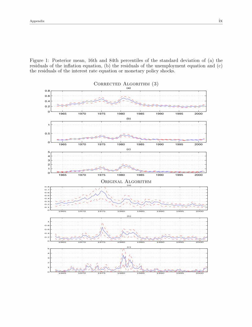
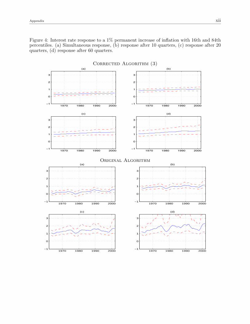
The first thing to notice is that the results based on Algorithm 3 are qualitatively similar

to the original ones obtained with Algorithm 1, but they are not the same (figures 1-8). The

main difference is that some estimates of the time-varying objects are now smoother. For

example, the standard deviation of monetary policy shocks (figure 1c) exhibits substantial

time variation, but not as much as in the original results. A similar comment applies to the

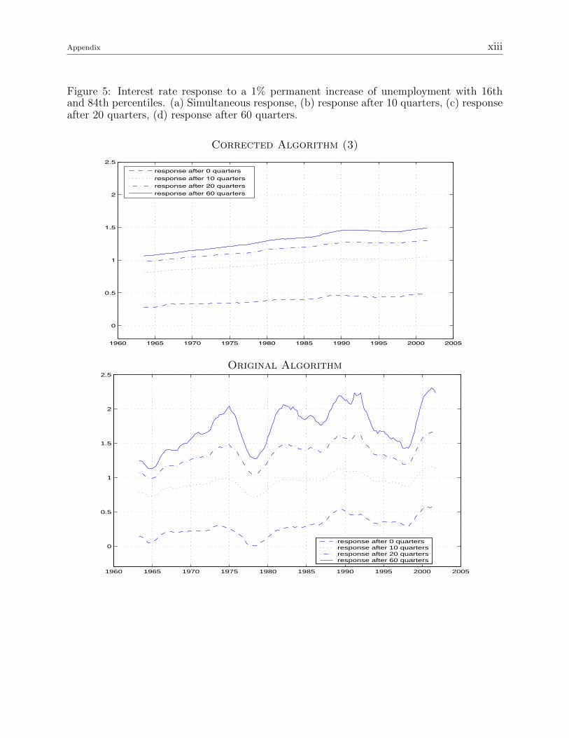
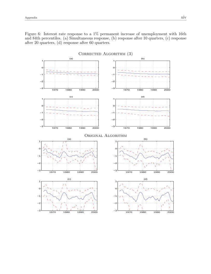
interest rate response to a permanent increase in inflation and unemployment (figures 5 and

7).

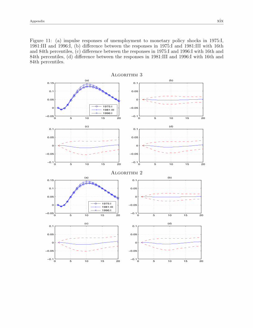
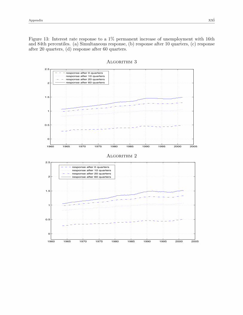
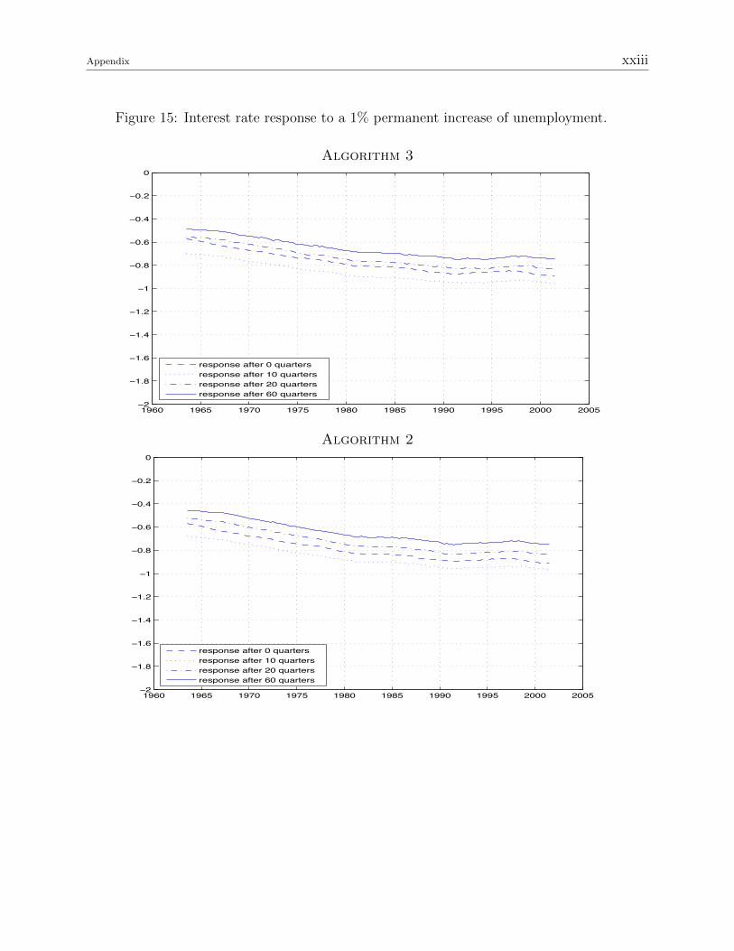
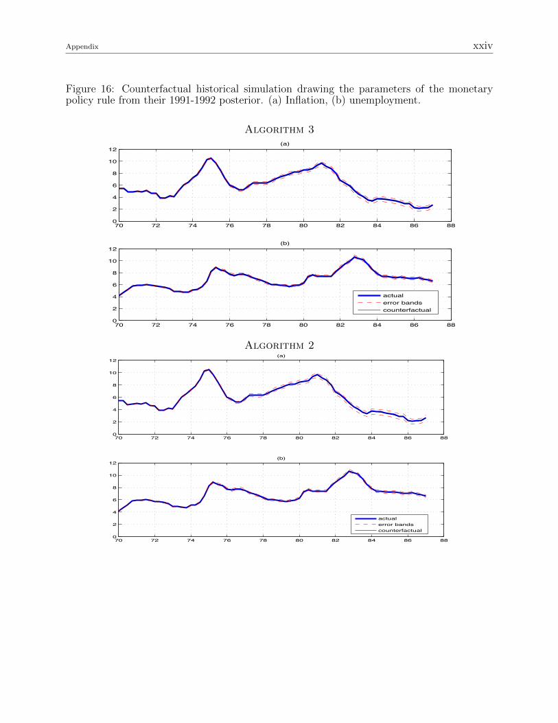
The results obtained using Algorithm 2 and 3 are instead indistinguishable from each

other (figures 9-16), suggesting that the mixture-of-normals approximation error involved

in the procedure of Kim, Shephard and Chib (1998, KSC hereafter) is negligible in our

application (as it was in theirs).

Appendix ii

B A Formal Treatment of Algorithm 2 and 3

In this section, we present a formal derivation of Algorithm 2 and 3.

B.1 Algorithm 2

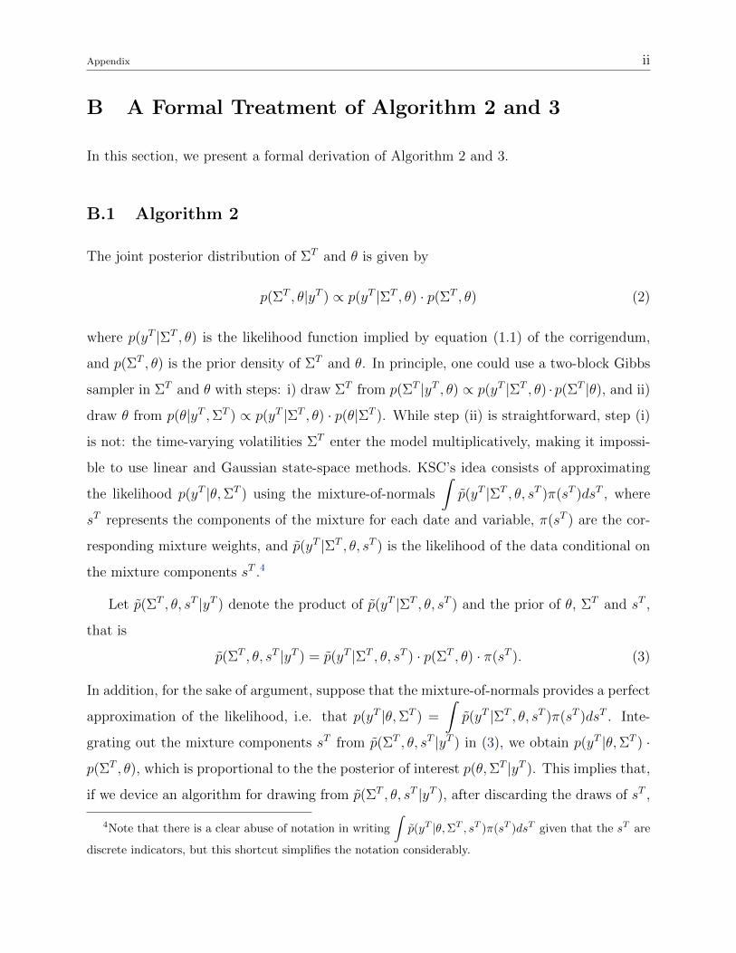
The joint posterior distribution of ΣT and θ is given by

p(ΣT , θ|yT ) ∝ p(yT |ΣT , θ) · p(ΣT , θ) (2)

where p(yT |ΣT , θ) is the likelihood function implied by equation (1.1) of the corrigendum,

and p(ΣT , θ) is the prior density of ΣT and θ. In principle, one could use a two-block Gibbs

sampler in ΣT and θ with steps: i) draw ΣT from p(ΣT |yT , θ) ∝ p(yT |ΣT , θ) ·p(ΣT |θ), and ii)

draw θ from p(θ|yT ,ΣT ) ∝ p(yT |ΣT , θ) · p(θ|ΣT ). While step (ii) is straightforward, step (i)

is not: the time-varying volatilities ΣT enter the model multiplicatively, making it impossi-

ble to use linear and Gaussian state-space methods. KSC’s idea consists of approximating

the likelihood p(yT |θ,ΣT ) using the mixture-of-normals

∫p(yT |ΣT , θ, sT )π(sT )dsT , where

sT represents the components of the mixture for each date and variable, π(sT ) are the cor-

responding mixture weights, and p(yT |ΣT , θ, sT ) is the likelihood of the data conditional on

the mixture components sT .4

Let p(ΣT , θ, sT |yT ) denote the product of p(yT |ΣT , θ, sT ) and the prior of θ, ΣT and sT ,

that is

p(ΣT , θ, sT |yT ) = p(yT |ΣT , θ, sT ) · p(ΣT , θ) · π(sT ). (3)

In addition, for the sake of argument, suppose that the mixture-of-normals provides a perfect

approximation of the likelihood, i.e. that p(yT |θ,ΣT ) =

∫p(yT |ΣT , θ, sT )π(sT )dsT . Inte-

grating out the mixture components sT from p(ΣT , θ, sT |yT ) in (3), we obtain p(yT |θ,ΣT ) ·

p(ΣT , θ), which is proportional to the the posterior of interest p(θ,ΣT |yT ). This implies that,

if we device an algorithm for drawing from p(ΣT , θ, sT |yT ), after discarding the draws of sT ,

4Note that there is a clear abuse of notation in writing

∫p(yT |θ,ΣT , sT )π(sT )dsT given that the sT are

discrete indicators, but this shortcut simplifies the notation considerably.

Appendix iii

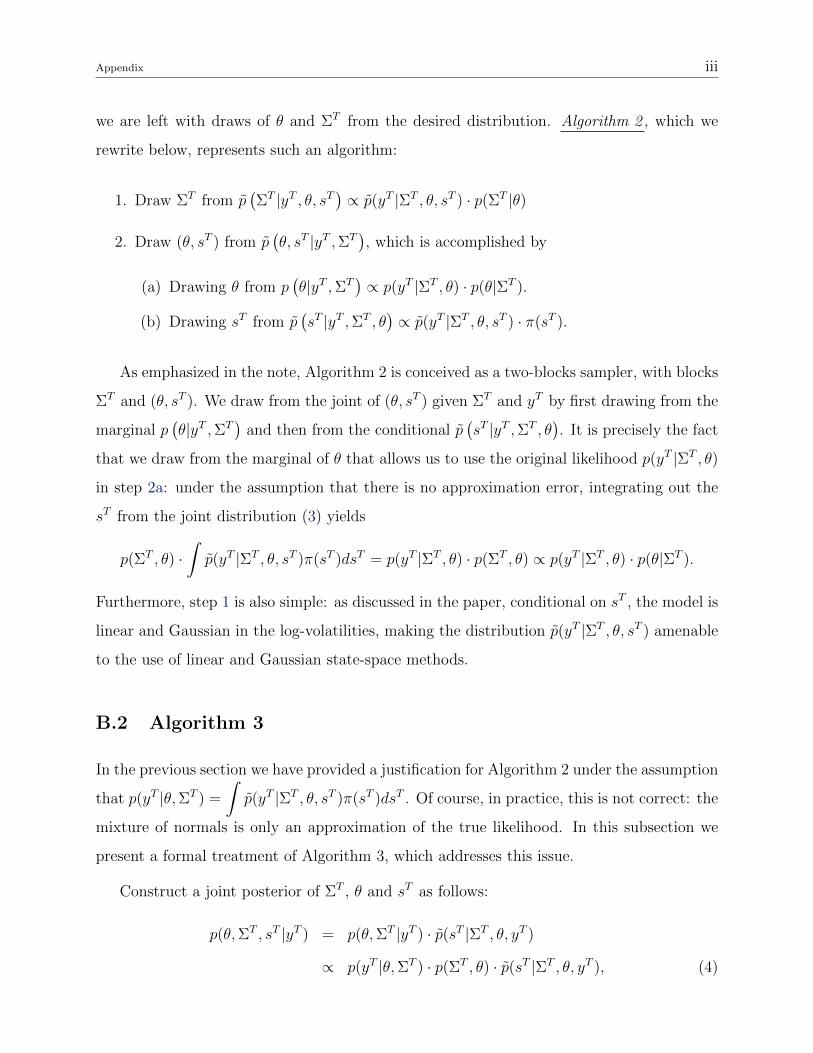
we are left with draws of θ and ΣT from the desired distribution. Algorithm 2 , which we

rewrite below, represents such an algorithm:


)∝ p(yT |ΣT , θ, sT ) · p(ΣT |θ)

2. Draw (θ, sT ) from p(θ, sT |yT ,ΣT


(a) Drawing θ from p(θ|yT ,ΣT

)∝ p(yT |ΣT , θ) · p(θ|ΣT ).

(b) Drawing sT from p(sT |yT ,ΣT , θ

)∝ p(yT |ΣT , θ, sT ) · π(sT ).

As emphasized in the note, Algorithm 2 is conceived as a two-blocks sampler, with blocks

ΣT and (θ, sT ). We draw from the joint of (θ, sT ) given ΣT and yT by first drawing from the

marginal p(θ|yT ,ΣT

)and then from the conditional p

(sT |yT ,ΣT , θ

). It is precisely the fact

that we draw from the marginal of θ that allows us to use the original likelihood p(yT |ΣT , θ)

in step 2a: under the assumption that there is no approximation error, integrating out the

sT from the joint distribution (3) yields

p(ΣT , θ) ·∫p(yT |ΣT , θ, sT )π(sT )dsT = p(yT |ΣT , θ) · p(ΣT , θ) ∝ p(yT |ΣT , θ) · p(θ|ΣT ).

Furthermore, step 1 is also simple: as discussed in the paper, conditional on sT , the model is

linear and Gaussian in the log-volatilities, making the distribution p(yT |ΣT , θ, sT ) amenable

to the use of linear and Gaussian state-space methods.

B.2 Algorithm 3

In the previous section we have provided a justification for Algorithm 2 under the assumption

that p(yT |θ,ΣT ) =

∫p(yT |ΣT , θ, sT )π(sT )dsT . Of course, in practice, this is not correct: the

mixture of normals is only an approximation of the true likelihood. In this subsection we

present a formal treatment of Algorithm 3, which addresses this issue.

Construct a joint posterior of ΣT , θ and sT as follows:

p(θ,ΣT , sT |yT ) = p(θ,ΣT |yT ) · p(sT |ΣT , θ, yT )

∝ p(yT |θ,ΣT ) · p(ΣT , θ) · p(sT |ΣT , θ, yT ), (4)

Appendix iv

with

p(sT |ΣT , θ, yT ) =p(yT |ΣT , θ, sT ) · π(sT )

c(ΣT , θ, yT ), (5)

where c(ΣT , θ, yT ) ≡∫p(yT |ΣT , θ, sT )π(sT )dsT guarantees that the density in (5) integrates

to one.

As discussed above, a perfectly fine approach for obtaining draws from the posterior of

interest, p(θ,ΣT |yT ), is to sample from p(θ,ΣT , sT |yT ), and then discard the draws of sT .

This is precisely what Algorithm 3 does. Like Algorithm 2, Algorithm 3 has the structure

of a two-block sampler, with blocks ΣT and(θ, sT

). However, Algorithm 3 follows Stroud et

al. (2003) in using a Metropolis-Hastings step for drawing ΣT conditional on (θ, sT ), where

the proposal pdf is given by

p(ΣT |yT , θ, sT

)∝ p(yT |ΣT , θ, sT ) · p(ΣT |θ), (6)

which is the density used in step 1 of Algorithm 2.5

Specifically, Algorithm 3 consists of the following steps:


)as follows: Draw a candidate ΣT from the proposal

density p(ΣT |yT , θ, sT

)of Algorithm 2, and set

Σ(j) T =

ΣT with probability α

Σ(j−1) T with probability 1− α,

where the superscript (j) denotes the iteration of the sampler, and where

α =p(

ΣT |yT , θ, sT)

p (Σ(j−1) T |yT , θ, sT )

p(Σ(j−1) T |yT , θ, sT

)p(

ΣT |yT , θ, sT) .

2. Draw (θ, sT ) from p(θ, sT |yT ,ΣT


(a) Drawing θ from

p(θ|yT ,ΣT

)=

∫p(θ, sT |yT ,ΣT )dsT

∝ p(yT |θ,ΣT ) · p(θ|ΣT ) ·∫p(sT |ΣT , θ, yT )dsT = p(yT |ΣT , θ) · p(θ|ΣT ).

5Stroud et al. (2003) study the use of mixture approximations in Gibbs samplers, and thus generalize

the results of KSC.

Appendix v

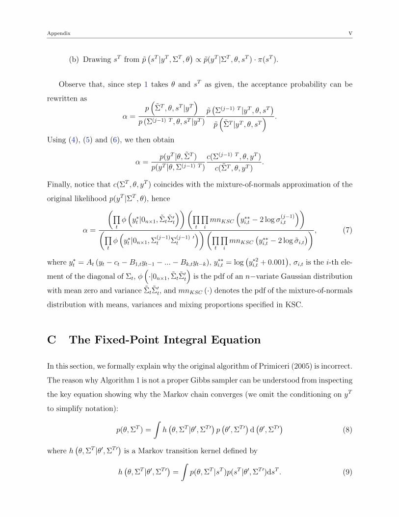
(b) Drawing sT from p(sT |yT ,ΣT , θ

)∝ p(yT |ΣT , θ, sT ) · π(sT ).

Observe that, since step 1 takes θ and sT as given, the acceptance probability can be

rewritten as

α =p(

ΣT , θ, sT |yT)

p (Σ(j−1) T , θ, sT |yT )

p(Σ(j−1) T |yT , θ, sT

)p(

ΣT |yT , θ, sT) .

Using (4), (5) and (6), we then obtain

α =p(yT |θ, ΣT )

p(yT |θ,Σ(j−1) T )

c(Σ(j−1) T , θ, yT )

c(ΣT , θ, yT ).

Finally, notice that c(ΣT , θ, yT ) coincides with the mixture-of-normals approximation of the

original likelihood p(yT |ΣT , θ), hence

α =

(∏t

φ(y∗t |0n×1, ΣtΣ

′t

))(∏t

∏i

mnKSC

(y∗∗i,t − 2 log σ

(j−1)i,t

))(∏

t

φ(y∗t |0n×1,Σ

(j−1)t Σ

(j−1) ′t

))(∏t

∏i

mnKSC

(y∗∗i,t − 2 log σi,t

)) , (7)

where y∗t = At (yt − ct −B1,tyt−1 − ...−Bk,tyt−k), y∗∗i,t = log(y∗2i,t + 0.001

), σi,t is the i-th ele-

ment of the diagonal of Σt, φ(·|0n×1, ΣtΣ

′t

)is the pdf of an n−variate Gaussian distribution

with mean zero and variance ΣtΣ′t, and mnKSC (·) denotes the pdf of the mixture-of-normals

distribution with means, variances and mixing proportions specified in KSC.

C The Fixed-Point Integral Equation

In this section, we formally explain why the original algorithm of Primiceri (2005) is incorrect.

The reason why Algorithm 1 is not a proper Gibbs sampler can be understood from inspecting

the key equation showing why the Markov chain converges (we omit the conditioning on yT

to simplify notation):

p(θ,ΣT ) =

∫h(θ,ΣT |θ′,ΣT ′) p (θ′,ΣT ′) d

(θ′,ΣT ′) (8)

where h(θ,ΣT |θ′,ΣT ′) is a Markov transition kernel defined by

h(θ,ΣT |θ′,ΣT ′) =

∫p(θ,ΣT |sT )p(sT |θ′,ΣT ′)dsT . (9)

Appendix vi

Equation (8) defines a fixed point integral equation for which the true marginal p(θ,ΣT ) is

a solution, which is readily seen by plugging (9) into (8) and changing the order of integra-

tion, as shown below (Chib and Greenberg, 1996 and references therein discuss why i) it is

the unique solution, and ii) there is convergence from any initial p(θ′,ΣT ′) under general

conditions). Omitting to condition on sT when drawing from p(θ,ΣT |sT ) (as done in step

3) implies using the wrong kernel, hence the fixed point argument breaks down: even if one

were to draw (θ′,ΣT ′) from the correct joint distribution, the resulting (θ,ΣT ) in the next

iteration would not be from p(θ,ΣT ).

In the three-block Gibbs sampler, equation (3.1)—the fixed point integral equation—

becomes

p(θ,ΣT , sT ) =

∫..

∫h(θ,ΣT , sT |θ′

,ΣT ′, sT

′)p(θ′,ΣT ′

, sT′)

dθ′dΣT ′

dsT′

(10)

where h(θ,ΣT , sT |θ′

,ΣT ′, sT

′)

is a Markov transition kernel defined by

h(θ,ΣT , sT |θ′

,ΣT ′, sT

′)

= p(θ|ΣT , sT )p(ΣT |θ′, sT )p(sT |θ′,ΣT ′

). (11)

Here we follow Chib and Greenberg (1996) and show that p(θ,ΣT , sT ) is indeed the solution

to (10). In fact, one can write the right hand side of expression (10), after substituting in

the definition of the transition kernel (11), as:∫..

∫p(θ|ΣT , sT )p(ΣT |θ′, sT )p(sT |θ′

,ΣT ′)p(θ′,ΣT ′

, sT′)

dθ′dΣT ′

dsT′=∫

..

∫p(θ|ΣT , sT )

p(ΣT |sT )p(θ′|ΣT , sT )

p(θ′|sT )

p(sT )p(θ′,ΣT ′|sT )

p(θ′ ,ΣT ′)p(θ′,ΣT ′

, sT′)

dθ′dΣT ′

dsT′

where we used Bayes law to express p(ΣT |θ′, sT ) and p(sT |θ′,ΣT ′

). Note that the terms

p(θ|ΣT , sT )p(ΣT |sT )p(sT ) = p(θ,ΣT , sT )

can be taken out of the integral as they do not depend on the ′ variables, and their product

is precisely p(θ,ΣT , sT ). Therefore we just have to show that∫..

∫p(θ′|ΣT , sT )

p(θ′|sT )

p(θ′,ΣT ′|sT )

p(θ′ ,ΣT ′)p(θ′,ΣT ′

, sT′)

dθ′dΣT ′

dsT′= 1.

Appendix vii

This is the case because∫..


p(θ′|sT )

p(θ′,ΣT ′|sT )

p(θ′ ,ΣT ′)p(θ

′,ΣT ′

, sT′)dθ

′dΣT ′

dsT′=∫

..


p(θ′|sT )

p(θ′ |sT )p(ΣT ′|θ′

, sT )

p(θ′ ,ΣT ′)p(θ

′,ΣT ′

)p(sT′ |θ′

,ΣT ′)dθ

′dΣT ′

dsT′=∫

p(θ′|ΣT , sT )

(∫p(ΣT ′ |θ′

, sT )

(∫p(sT

′|ΣT ′, sT

′)dsT

′)

dΣT ′)

dθ′= 1,

where in the second line we again used Bayes law and in the fourth line we realized that

we are left with three conditional distributions, all integrating to one. Clearly, omitting to

condition on sT when drawing from p(θ|ΣT , sT

)implies using the wrong kernel, and the

fixed-point arguments breaks down.

D Geweke’s (2004) “Getting It Right”

In this section, we apply Geweke’s (2004) “Joint Distribution Tests of Posterior Simulators”

to the three algorithms discussed in the note, and present further evidence that Algorithm

1 is wrong, Algorithm 2 is approximately correct, and Algorithm 3 is correct. Geweke’s idea

is to compare two ways of obtaining draws from the joint distribution of the data and the

model parameters, p(yT , θ,ΣT , sT

):

a. Draw the parameters from the prior, and then the data from the data-generating

process (that is, draw sequentially from p(θ,ΣT , sT

)and p

(yT |θ,ΣT , sT

)).

b. Draw from the posterior using the MCMC algorithm given a draw of the data, and then

use this draw to generate another draw from data, and so on (that is, draw sequentially

from p(θ,ΣT , sT |yT

)and then from p

(yT |θ,ΣT , sT

)).

If the MCMC algorithm is correct, (a) and (b) should yield the same distribution, and in

particular the same marginal for the model parameters (which, in the case of (a), is of course

the prior). Therefore, if the MCMC algorithm is correct, P-P plots constructed using the

draws from (a) and (b) should lie on the 45-degree line.

Appendix viii

We now present the results obtained by applying this procedure to the various algorithms

that we have discussed so far. Note that, for computational reasons, we use T = 10 in running

these tests, which is smaller than the actual sample size. For a T as large as that in the

sample, it simply takes so many draws for (b) to converge (even if the MCMC algorithm is

right) that the test is computationally not feasible. Since Geweke’s approach applies to any

T , we are justified in using a smaller T that makes the comparison feasible.

We concentrate on the P-P plots for the distribution of the log-volatilities at a particular

point in time (t = 7), because the differences are smaller for the other coefficients. Figure 17

shows the results related to the original algorithm (Algorithm 1). It is evident that the P-P

plots are very far from the 45-degree line, indicating that the draws generated with (a) and

(b) belong to different distributions. This suggests the presence of a mistake in Algorithm

1, as we have argued above.

Figure 18 plots the results obtained using Algorithm 2. The fact that the P-P plots in

figure 18 are now much closer to the 45-degree line is a sign of dramatic improvement in

the accuracy of the algorithm. The natural question is of course why these P-P plots do

not lie exactly on top of the 45-degree line, but just close to it. This is due to the minor

error involved in the mixture-of-normals approximation proposed by KSC. A property of

the Geweke (2004) approach is that it amplifies subtle discrepancies in the sampler, such as

these small approximation errors. Figure 19 confirms this conjecture by presenting the P-P

plots obtained by running the Geweke procedure using Algorithm 3. In this case, the P-P

plots essentially coincide with the 45-degree lines, which verifies that there is no problem

with Algorithm 2, other than the fact that it uses the mixture approximation to increase effi-

ciency and speed of convergence. Recall from section 1 that this approximation is absolutely

inconsequential for the estimation results, i.e. for the construction the posterior distribution

given the observed data. Conversely, applying the same correction for the mixture-of-normals

approximation error in step 1 of the original algorithm does not improve the P-P plots at

all, as shown in figure 20.

Appendix ix

Figure 1: Posterior mean, 16th and 84th percentiles of the standard deviation of (a) theresiduals of the inflation equation, (b) the residuals of the unemployment equation and (c)the residuals of the interest rate equation or monetary policy shocks.

Corrected Algorithm (3)

1965 1970 1975 1980 1985 1990 1995 20000

0.2

0.4

0.6

0.8(a)

1965 1970 1975 1980 1985 1990 1995 20000

0.5

1

(b)

1965 1970 1975 1980 1985 1990 1995 2000012345

(c)

Original Algorithm

1965 1970 1975 1980 1985 1990 1995 20000

0.1

0.2

0.3

0.4

0.5

0.6

0.7

0.8(a)

1965 1970 1975 1980 1985 1990 1995 20000

0.2

0.4

0.6

0.8

1

(b)

1965 1970 1975 1980 1985 1990 1995 20000

1

2

3

4

5(c)

Appendix x

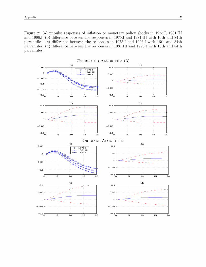
Figure 2: (a) impulse responses of inflation to monetary policy shocks in 1975:I, 1981:IIIand 1996:I, (b) difference between the responses in 1975:I and 1981:III with 16th and 84thpercentiles, (c) difference between the responses in 1975:I and 1996:I with 16th and 84thpercentiles, (d) difference between the responses in 1981:III and 1996:I with 16th and 84thpercentiles.


0 5 10 15 20−0.2

−0.15

−0.1

−0.05

0

0.05(a)

0 5 10 15 20−0.1

−0.05

0

0.05

0.1(b)

0 5 10 15 20−0.1

−0.05

0

0.05

0.1(c)

1975:I1981:III1996:I

0 5 10 15 20−0.1

−0.05

0

0.05

0.1(d)

Original Algorithm

0 5 10 15 20

−0.1

−0.05

0

0.05(a)

1975:I1981:III1996:I

0 5 10 15 20−0.1

−0.05

0

0.05

0.1(b)

0 5 10 15 20−0.1

−0.05

0

0.05

0.1(c)

0 5 10 15 20−0.1

−0.05

0

0.05

0.1(d)

Appendix xi

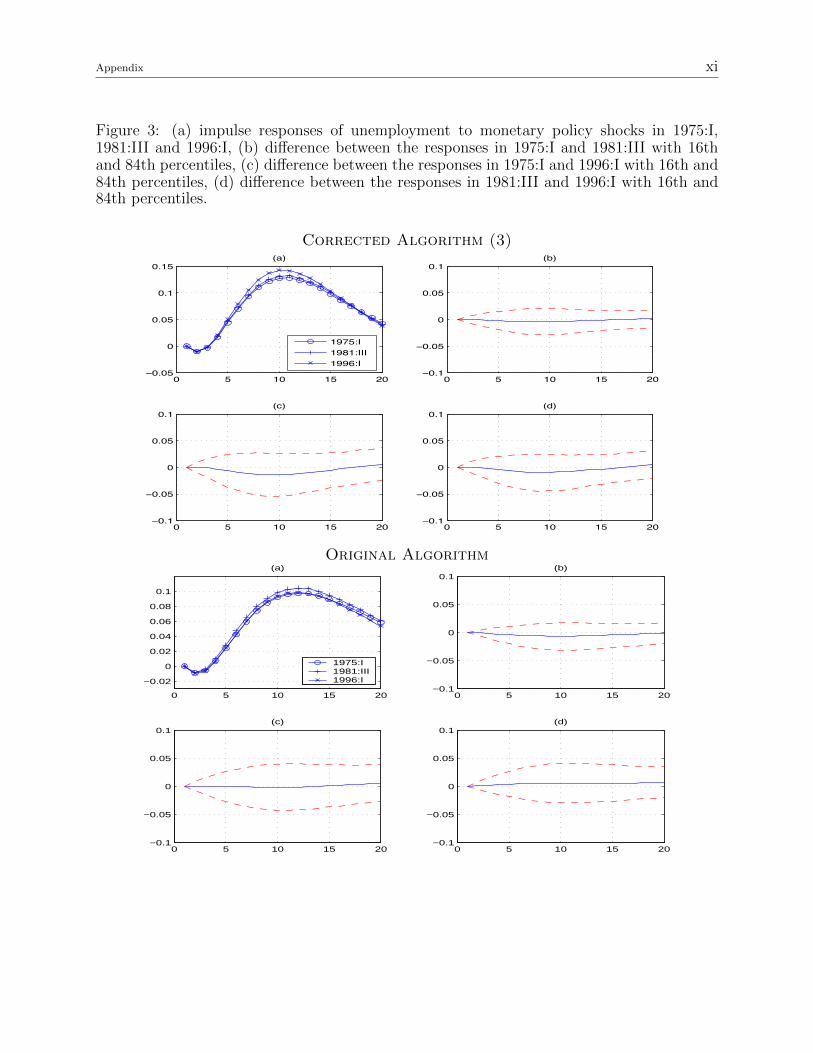
Figure 3: (a) impulse responses of unemployment to monetary policy shocks in 1975:I,1981:III and 1996:I, (b) difference between the responses in 1975:I and 1981:III with 16thand 84th percentiles, (c) difference between the responses in 1975:I and 1996:I with 16th and84th percentiles, (d) difference between the responses in 1981:III and 1996:I with 16th and84th percentiles.


0 5 10 15 20−0.05

0

0.05

0.1

0.15(a)

0 5 10 15 20−0.1

−0.05

0

0.05

0.1(b)

0 5 10 15 20−0.1

−0.05

0

0.05

0.1(c)

1975:I1981:III1996:I

0 5 10 15 20−0.1

−0.05

0

0.05

0.1(d)

Original Algorithm

0 5 10 15 20

−0.02

0

0.02

0.04

0.06

0.08

0.1

(a)

1975:I1981:III1996:I

0 5 10 15 20−0.1

−0.05

0

0.05

0.1(b)

0 5 10 15 20−0.1

−0.05

0

0.05

0.1(c)

0 5 10 15 20−0.1

−0.05

0

0.05

0.1(d)

Appendix xii

Figure 4: Interest rate response to a 1% permanent increase of inflation with 16th and 84thpercentiles. (a) Simultaneous response, (b) response after 10 quarters, (c) response after 20quarters, (d) response after 60 quarters.


1970 1980 1990 2000−1

0

1

2

3

(a)

1970 1980 1990 2000−1

0

1

2

3

(b)

1970 1980 1990 2000−1

0

1

2

3

(c)

1970 1980 1990 2000−1

0

1

2

3

(d)

Original Algorithm

1970 1980 1990 2000−1

0

1

2

3

(a)

1970 1980 1990 2000−1

0

1

2

3

(b)

1970 1980 1990 2000−1

0

1

2

3

(c)

1970 1980 1990 2000−1

0

1

2

3

(d)

Appendix xiii

Figure 5: Interest rate response to a 1% permanent increase of unemployment with 16thand 84th percentiles. (a) Simultaneous response, (b) response after 10 quarters, (c) responseafter 20 quarters, (d) response after 60 quarters.


1960 1965 1970 1975 1980 1985 1990 1995 2000 2005

0

0.5

1

1.5

2

2.5

response after 0 quartersresponse after 10 quartersresponse after 20 quartersresponse after 60 quarters

Original Algorithm

1960 1965 1970 1975 1980 1985 1990 1995 2000 2005

0

0.5

1

1.5

2

2.5


Appendix xiv



1970 1980 1990 2000−3

−2

−1

0

1(a)

1970 1980 1990 2000−3

−2

−1

0

1(b)

1970 1980 1990 2000−3

−2

−1

0

1(c)

1970 1980 1990 2000−3

−2

−1

0

1(d)

Original Algorithm

1970 1980 1990 2000−3

−2

−1

0

1(a)

1970 1980 1990 2000−3

−2

−1

0

1(b)

1970 1980 1990 2000−3

−2

−1

0

1(c)

1970 1980 1990 2000−3

−2

−1

0

1(d)

Appendix xv

Figure 7: Interest rate response to a 1% permanent increase of unemployment.


1960 1965 1970 1975 1980 1985 1990 1995 2000 2005−2

−1.8

−1.6

−1.4

−1.2

−1

−0.8

−0.6

−0.4

−0.2

0


Original Algorithm

1960 1965 1970 1975 1980 1985 1990 1995 2000 2005−2

−1.8

−1.6

−1.4

−1.2

−1

−0.8

−0.6

−0.4

−0.2

0response after 0 quartersresponse after 10 quartersresponse after 20 quartersresponse after 60 quarters

Appendix xvi

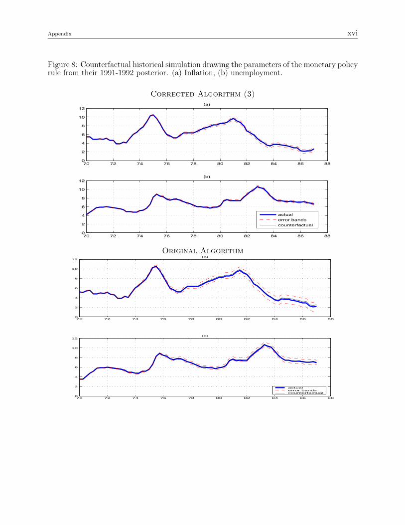
Figure 8: Counterfactual historical simulation drawing the parameters of the monetary policyrule from their 1991-1992 posterior. (a) Inflation, (b) unemployment.


70 72 74 76 78 80 82 84 86 880

2

4

6

8

10

12(a)

70 72 74 76 78 80 82 84 86 880

2

4

6

8

10

12(b)

actualerror bandscounterfactual

Original Algorithm

70 72 74 76 78 80 82 84 86 880

2

4

6

8

10

12(a)

70 72 74 76 78 80 82 84 86 880

2

4

6

8

10

12(b)


Appendix xvii

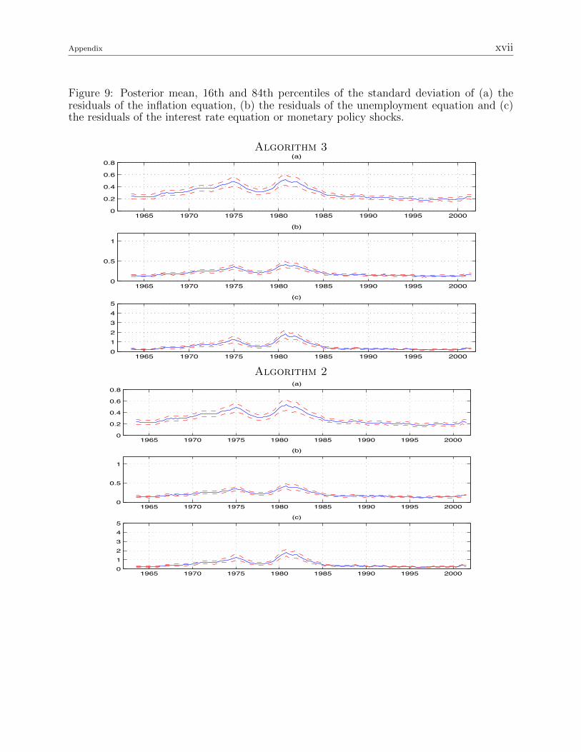
Figure 9: Posterior mean, 16th and 84th percentiles of the standard deviation of (a) theresiduals of the inflation equation, (b) the residuals of the unemployment equation and (c)the residuals of the interest rate equation or monetary policy shocks.

Algorithm 3

1965 1970 1975 1980 1985 1990 1995 20000

0.2

0.4

0.6

0.8(a)

1965 1970 1975 1980 1985 1990 1995 20000

0.5

1

(b)

1965 1970 1975 1980 1985 1990 1995 2000012345

(c)

Algorithm 2

1965 1970 1975 1980 1985 1990 1995 20000

0.2

0.4

0.6

0.8(a)

1965 1970 1975 1980 1985 1990 1995 20000

0.5

1

(b)

1965 1970 1975 1980 1985 1990 1995 2000012345

(c)

Appendix xviii

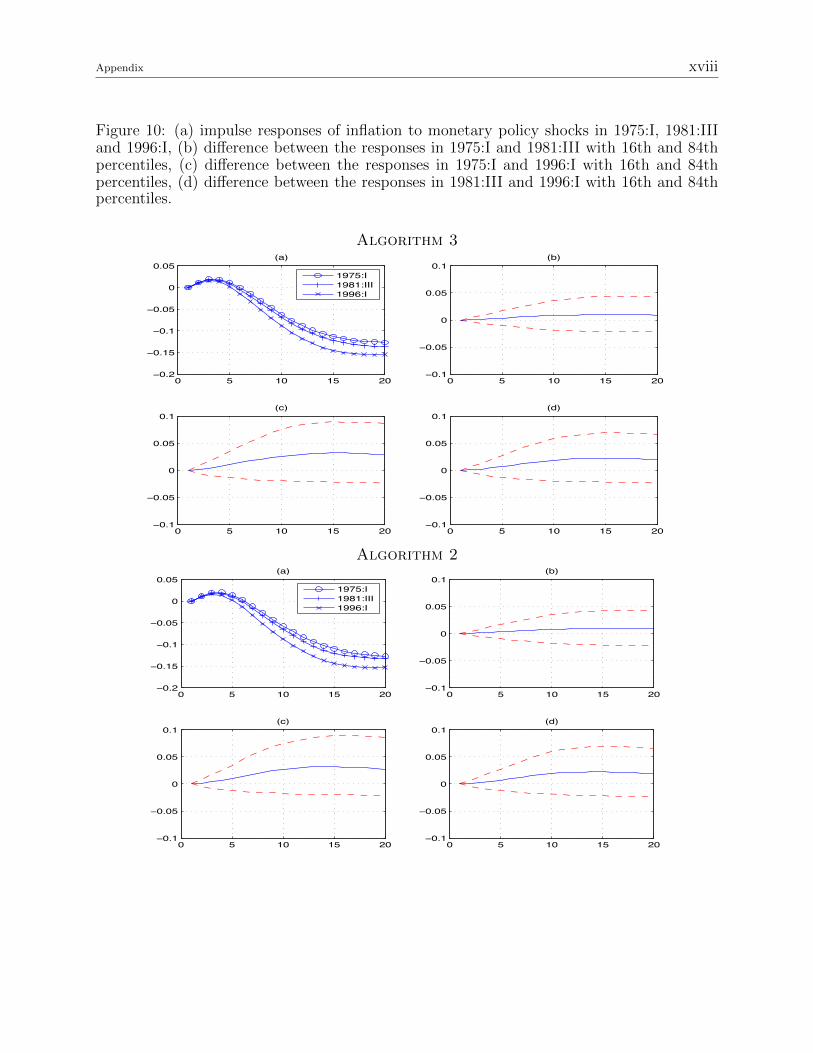
Figure 10: (a) impulse responses of inflation to monetary policy shocks in 1975:I, 1981:IIIand 1996:I, (b) difference between the responses in 1975:I and 1981:III with 16th and 84thpercentiles, (c) difference between the responses in 1975:I and 1996:I with 16th and 84thpercentiles, (d) difference between the responses in 1981:III and 1996:I with 16th and 84thpercentiles.

Algorithm 3

0 5 10 15 20−0.2

−0.15

−0.1

−0.05

0

0.05(a)

0 5 10 15 20−0.1

−0.05

0

0.05

0.1(b)

0 5 10 15 20−0.1

−0.05

0

0.05

0.1(c)

1975:I1981:III1996:I

0 5 10 15 20−0.1

−0.05

0

0.05

0.1(d)

Algorithm 2

0 5 10 15 20−0.2

−0.15

−0.1

−0.05

0

0.05(a)

0 5 10 15 20−0.1

−0.05

0

0.05

0.1(b)

0 5 10 15 20−0.1

−0.05

0

0.05

0.1(c)

1975:I1981:III1996:I

0 5 10 15 20−0.1

−0.05

0

0.05

0.1(d)

Appendix xix

Figure 11: (a) impulse responses of unemployment to monetary policy shocks in 1975:I,1981:III and 1996:I, (b) difference between the responses in 1975:I and 1981:III with 16thand 84th percentiles, (c) difference between the responses in 1975:I and 1996:I with 16th and84th percentiles, (d) difference between the responses in 1981:III and 1996:I with 16th and84th percentiles.

Algorithm 3

0 5 10 15 20−0.05

0

0.05

0.1

0.15(a)

0 5 10 15 20−0.1

−0.05

0

0.05

0.1(b)

0 5 10 15 20−0.1

−0.05

0

0.05

0.1(c)

1975:I1981:III1996:I

0 5 10 15 20−0.1

−0.05

0

0.05

0.1(d)

Algorithm 2

0 5 10 15 20−0.05

0

0.05

0.1

0.15(a)

0 5 10 15 20−0.1

−0.05

0

0.05

0.1(b)

0 5 10 15 20−0.1

−0.05

0

0.05

0.1(c)

1975:I1981:III1996:I

0 5 10 15 20−0.1

−0.05

0

0.05

0.1(d)

Appendix xx

Figure 12: Interest rate response to a 1% permanent increase of inflation with 16th and 84thpercentiles. (a) Simultaneous response, (b) response after 10 quarters, (c) response after 20quarters, (d) response after 60 quarters.

Algorithm 3

1970 1980 1990 2000−1

0

1

2

3

(a)

1970 1980 1990 2000−1

0

1

2

3

(b)

1970 1980 1990 2000−1

0

1

2

3

(c)

1970 1980 1990 2000−1

0

1

2

3

(d)

Algorithm 2

1970 1980 1990 2000−1

0

1

2

3

(a)

1970 1980 1990 2000−1

0

1

2

3

(b)

1970 1980 1990 2000−1

0

1

2

3

(c)

1970 1980 1990 2000−1

0

1

2

3

(d)

Appendix xxi


Algorithm 3

1960 1965 1970 1975 1980 1985 1990 1995 2000 2005

0

0.5

1

1.5

2

2.5


Algorithm 2

1960 1965 1970 1975 1980 1985 1990 1995 2000 2005

0

0.5

1

1.5

2

2.5


Appendix xxii


Algorithm 3

1970 1980 1990 2000−3

−2

−1

0

1(a)

1970 1980 1990 2000−3

−2

−1

0

1(b)

1970 1980 1990 2000−3

−2

−1

0

1(c)

1970 1980 1990 2000−3

−2

−1

0

1(d)

Algorithm 2

1970 1980 1990 2000−3

−2

−1

0

1(a)

1970 1980 1990 2000−3

−2

−1

0

1(b)

1970 1980 1990 2000−3

−2

−1

0

1(c)

1970 1980 1990 2000−3

−2

−1

0

1(d)

Appendix xxiii

Figure 15: Interest rate response to a 1% permanent increase of unemployment.

Algorithm 3

1960 1965 1970 1975 1980 1985 1990 1995 2000 2005−2

−1.8

−1.6

−1.4

−1.2

−1

−0.8

−0.6

−0.4

−0.2

0


Algorithm 2

1960 1965 1970 1975 1980 1985 1990 1995 2000 2005−2

−1.8

−1.6

−1.4

−1.2

−1

−0.8

−0.6

−0.4

−0.2

0


Appendix xxiv

Figure 16: Counterfactual historical simulation drawing the parameters of the monetarypolicy rule from their 1991-1992 posterior. (a) Inflation, (b) unemployment.

Algorithm 3

70 72 74 76 78 80 82 84 86 880

2

4

6

8

10

12(a)

70 72 74 76 78 80 82 84 86 880

2

4

6

8

10

12(b)


Algorithm 2

70 72 74 76 78 80 82 84 86 880

2

4

6

8

10

12(a)

70 72 74 76 78 80 82 84 86 880

2

4

6

8

10

12(b)


Appendix xxv

Figure 17: P-P plots obtained by applying the Geweke’s (2004) procedure to Algorithm 1.The plots refer to the distribution of log σi,t, with t = 7, and i = 1 in panel (a), i = 2 inpanel (b), and i = 3 in panel (c).

0 0.2 0.4 0.6 0.8 10

0.2

0.4

0.6

0.8

1a

0 0.2 0.4 0.6 0.8 10

0.2

0.4

0.6

0.8

1b

0 0.2 0.4 0.6 0.8 10

0.2

0.4

0.6

0.8

1c

P−P plot

45−degree line


0 0.2 0.4 0.6 0.8 10

0.2

0.4

0.6

0.8

1a

0 0.2 0.4 0.6 0.8 10

0.2

0.4

0.6

0.8

1b

0 0.2 0.4 0.6 0.8 10

0.2

0.4

0.6

0.8

1c

P−P plot

45−degree line

Appendix xxvi


0 0.2 0.4 0.6 0.8 10

0.2

0.4

0.6

0.8

1a

0 0.2 0.4 0.6 0.8 10

0.2

0.4

0.6

0.8

1b

0 0.2 0.4 0.6 0.8 10

0.2

0.4

0.6

0.8

1c

P−P plot

45−degree line

Figure 20: P-P plots obtained by applying the Geweke’s (2004) procedure to Algorithm 1augmented with a Metropolis-Hastings step to correct for the mixture-of-normals approxi-mation error. The plots refer to the distribution of log σi,t, with t = 7, and i = 1 in panel(a), i = 2 in panel (b), and i = 3 in panel (c).

0 0.2 0.4 0.6 0.8 10

0.2

0.4

0.6

0.8

1a

0 0.2 0.4 0.6 0.8 10

0.2

0.4

0.6

0.8

1b

0 0.2 0.4 0.6 0.8 10

0.2

0.4

0.6

0.8

1c

P−P plot

45−degree line

Time-Varying Structural Vector Autoregressions and ... · distribution of the model coe cients by...

Documents

Transcript of Time-Varying Structural Vector Autoregressions and ... · distribution of the model coe cients by...