
TIME-VARYING COEFFICIENT MODELS FOR JOINT MODELING …
24
TIME-VARYING COEFFICIENT MODELS FOR JOINT MODELING BINARY AND CONTINUOUS OUTCOMES IN LONGITUDINAL DATA Esra Kürüm 1 , Runze Li 2 , Saul Shiffman 3 , and Weixin Yao 4 Esra Kürüm: [email protected]; Runze Li: [email protected]; Saul Shiffman: [email protected]; Weixin Yao: [email protected] 1 Department of Epidemiology of Microbial Diseases, Yale School of Public Health, New Haven, CT 06520, U.S.A 2 Department of Statistics and The Methodology Center, The Pennsylvania State University, University Park, PA 16802-2111, U.S.A. 3 Department of Psychology, University of Pittsburgh, Pittsburgh, PA 15260,U.S.A. 4 Department of Statistics, University of California, Riverside, California 92521, U.S.A. Abstract Motivated by an empirical analysis of ecological momentary assessment data (EMA) collected in a smoking cessation study, we propose a joint modeling technique for estimating the time-varying association between two intensively measured longitudinal responses: a continuous one and a binary one. A major challenge in joint modeling these responses is the lack of a multivariate distribution. We suggest introducing a normal latent variable underlying the binary response and factorizing the model into two components: a marginal model for the continuous response, and a conditional model for the binary response given the continuous response. We develop a two-stage estimation procedure and establish the asymptotic normality of the resulting estimators. We also derived the standard error formulas for estimated coefficients. We conduct a Monte Carlo simulation study to assess the finite sample performance of our procedure. The proposed method is illustrated by an empirical analysis of smoking cessation data, in which the question of interest is to investigate the association between urge to smoke, continuous response, and the status of alcohol use, the binary response, and how this association varies over time. Key words and phrases Generalized linear models; Local linear regression; Varying coefficient models Corresponding Author. Esra Kurum, [email protected]. Supplementary Materials Supplementary materials include proofs of the theorems of Section 2.3. HHS Public Access Author manuscript Stat Sin. Author manuscript; available in PMC 2017 July 01. Published in final edited form as: Stat Sin. 2016 July ; 26(3): 979–1000. doi:10.5705/ss.2014.213. Author Manuscript Author Manuscript Author Manuscript Author Manuscript
Transcript of TIME-VARYING COEFFICIENT MODELS FOR JOINT MODELING …

TIME-VARYING COEFFICIENT MODELS FOR JOINT MODELING BINARY AND CONTINUOUS OUTCOMES IN LONGITUDINAL DATA
Esra Kürüm1, Runze Li2, Saul Shiffman3, and Weixin Yao4
Esra Kürüm: [email protected]; Runze Li: [email protected]; Saul Shiffman: [email protected]; Weixin Yao: [email protected] of Epidemiology of Microbial Diseases, Yale School of Public Health, New Haven, CT 06520, U.S.A
2Department of Statistics and The Methodology Center, The Pennsylvania State University, University Park, PA 16802-2111, U.S.A.
3Department of Psychology, University of Pittsburgh, Pittsburgh, PA 15260,U.S.A.
4Department of Statistics, University of California, Riverside, California 92521, U.S.A.
Abstract
Motivated by an empirical analysis of ecological momentary assessment data (EMA) collected in a
smoking cessation study, we propose a joint modeling technique for estimating the time-varying
association between two intensively measured longitudinal responses: a continuous one and a
binary one. A major challenge in joint modeling these responses is the lack of a multivariate
distribution. We suggest introducing a normal latent variable underlying the binary response and
factorizing the model into two components: a marginal model for the continuous response, and a
conditional model for the binary response given the continuous response. We develop a two-stage
estimation procedure and establish the asymptotic normality of the resulting estimators. We also
derived the standard error formulas for estimated coefficients. We conduct a Monte Carlo
simulation study to assess the finite sample performance of our procedure. The proposed method
is illustrated by an empirical analysis of smoking cessation data, in which the question of interest
is to investigate the association between urge to smoke, continuous response, and the status of
alcohol use, the binary response, and how this association varies over time.
Key words and phrases
Generalized linear models; Local linear regression; Varying coefficient models
Corresponding Author. Esra Kurum, [email protected].
Supplementary MaterialsSupplementary materials include proofs of the theorems of Section 2.3.
HHS Public AccessAuthor manuscriptStat Sin. Author manuscript; available in PMC 2017 July 01.
Published in final edited form as:Stat Sin. 2016 July ; 26(3): 979–1000. doi:10.5705/ss.2014.213.
Author M
anuscriptA
uthor Manuscript
Author M
anuscriptA
uthor Manuscript

1. Introduction
Early work on modeling longitudinal and clustered data focused on developing
methodologies for datasets with a single response. More recent studies have involved
multiple responses, often of mixed type, e.g., binary and continuous. The work was
motivated by an empirical analysis in Section 3.2, in which the data were collected
intensively during a smoking cessation study (Shiffman et al. (1996)) and contain multiple
responses such as urge to smoke (a continuous response), alcohol use, and presence of other
smokers (both binary responses). The latter two responses are of interest because it has been
observed that alcohol consumption and the presence of other smokers increase the odds of
smoking (Hymowitz et al. (1997); Shiffman and Balabanis (1995); Shiffman et al. (2002)),
and both have been associated with an increased risk of lapsing back to smoking (Kahler et
al. (2010); Shiffman et al. (2007)). Moreover, there is some hint that the relationship
between these stimuli and smoking (and therefore perhaps urge to smoke) may vary over
time, particularly weakening after the initial few days of abstinence. Our primary interest is
to estimate the time-varying association between these responses and urge to smoke so that
researchers can understand how the association between these variables changes during the
smoking cessation process. To estimate the association between the variables, we need to
model the variables jointly. Hence, we develop a new joint modeling method for longitudinal
binary and continuous responses, along with a corresponding estimation procedure.
The major difficulty in modeling binary and continuous responses jointly is the lack of a
natural multivariate distribution. To overcome this difficulty, many authors (Catalano and
Ryan (1992); Cox and Wermuth (1992); Dunson (2000); Fitzmaurice and Laird (1995);
Gueorguieva and Agresti (2001); Liu et al. (2009); Regan and Catalano (1999); Sammel et
al. (1997)) have employed what is now a well-known method, namely, introducing a
continuous latent variable underlying the binary response, and assuming that the latent
variable and the continuous response follow a joint normal distribution. After introducing
the latent variable, Catalano and Ryan (1992) suggested decomposing the joint distribution
into components that can be modeled separately: a marginal distribution for the continuous
response, and a conditional distribution for the binary response given the continuous
response. The first component is readily obtained, and the second component is obtained
using the assumption of joint normality.
Motivated by an empirical analysis in Section 3, we proposed time-varying coefficient
models for jointly modeling binary and continuous response. Time-varying coefficient
models have been introduced to model continuous response in both independent and
identically distributed (iid) data and longitudinal data (Hastie and Tibshirani (1993);
Brumback and Rice (1998); Hoover et al. (1998); Wu et al. (1998); Zhang and Lee (2000)),
and have been proposed for iid data with binary response (Cai et al. (2000)). To our best
knowledge, time-varying coefficient models have not been applied for jointly modeling
binary and continuous responses in longitudinal data setting. In this article we focus on
estimating the time-varying association between longitudinal binary and continuous
responses measured at the same time point within a subject.
Kürüm et al. Page 2
Stat Sin. Author manuscript; available in PMC 2017 July 01.
Author M
anuscriptA
uthor Manuscript
Author M
anuscriptA
uthor Manuscript

We propose an estimation procedure to time-varying coefficient model for jointly modeling
binary and responses outcomes in longitudinal data. Adapting from existing literature, we
introduce a continuous latent variable underlying the binary response, and we decompose
the joint distribution into two components. This leads to a two-stage estimation procedure.
In the first stage we fit the marginal model of the continuous response by using time-varying
coefficient models. In the second stage we use generalized time-varying coefficient models
(Cai et al. (2000) for iid data) to fit the conditional model of the binary response. We
systematically study the sampling property of the proposed estimation procedure, and
establish its asymptotic normality. The efficacy of our methodology is demonstrated by a
simulation study.
The remainder of the paper is organized as follows. In Section 2, we propose a joint model
for longitudinal binary and continuous responses, and further develop our two-stage
estimation procedure by using local linear regression techniques; we also study asymptotic
properties of the resulting estimators. In Section 3 we report on an extensive simulation
study to investigate the finite sample behavior of our estimators, and further illustrate the
proposed methodology by a data example. Regularity conditions and proofs are given in the
supplementary material.
2. Joint Models for Binary and Continuous Responses
We propose time-varying coefficient models for joint modeling binary and continuous
responses in Section 2.1. We propose an estimation procedure in Section 2.2, and study the
sampling property of the proposed estimate in Section 2.3.
2.1. Joint Models
We begin with notation. For the ith subject, i = 1, …, n, denote the binary response measured
at time point tij by Qi(tij), the continuous response by Wi(tij), where j = 1, …, ni. Define the
latent variable underlying Qi(tij) by Yi(tij). Let Xi(tij) = (Xi1(tij), …, Xip(tij))T be the vector
of predictors with Xi1 ≡ 1 to include an intercept term, β(tij) = (β1(tij), …, βp(tij))T, and
α(tij) = (α1(tij), …, αp(tij))T be the vectors of regression coefficients. Consider the bivariate
model:
(2.1)
where ε1i(t) and ε2i(t) are normal with mean zero and time-varying variances and
, respectively, strictly positive. We take εi(tij) = (ε1i(tij), ε2i(tij))T, and assume that εi(tij) is bivariate normal with corr {ε1i(tij), ε2i(tij)} = τ (tij). The relation between the latent
variable and the binary variable is defined as Qi(tij) = 1 if Yi(tij) > 0, and Qi(tij) = 0 if Yi(tij) ≤ 0. Thus, the probit model for the binary response Qi(tij) is
Kürüm et al. Page 3
Stat Sin. Author manuscript; available in PMC 2017 July 01.
Author M
anuscriptA
uthor Manuscript
Author M
anuscriptA
uthor Manuscript

The joint distribution of Wi(tij) and Qi(tij) is challenging to derive; however, the marginal
distributions are readily obtained. Thus, we factor the joint distribution of the continuous
variable and the binary variable into two components: a marginal model for the continuous
variable Wi(tij) and a conditional model for Qi(tij) given Wi(tij),
where j = 1, …, ni. The marginal model for the continuous response is defined in (2.1). To
derive the conditional model for Qi(tij) given Wi(tij), we start by obtaining the conditional
model Yi(tij) | Wi(tij). As standard normal theory shows, the conditional distribution Yi(tij) | Wi(tij) is Gaussian. The mean of this distribution depends on the error from the marginal
model of the continuous response, , where
(2.2)
is the error from the marginal model of the continuous
response. Thus,
(2.3)
where μi(tij) is defined in (2.2). The bivariate normal assumption for εi(tij) is only necessary
to obtain the conditional distribution of the binary response given the continuous response as
described in (2.3).
Not all parameters in (2.3) are estimable, hence we reparameterize (2.3) to the more
parsimonious and fully estimable form
(2.4)
where with r = 1, …, p. Model (2.4) links the
continuous response with the binary response in a probit regression model using the error
from the marginal model as a covariate. From the conditional model, it can be seen that
Kürüm et al. Page 4
Stat Sin. Author manuscript; available in PMC 2017 July 01.
Author M
anuscriptA
uthor Manuscript
Author M
anuscriptA
uthor Manuscript

Therefore, has the same sign as τ (tij) and increases when τ (tij) increases. Let
. Then
(2.5)
This joint modeling approach introduces time-varying effects to the well-known joint
modeling framework suggested by Catalano and Ryan (1992): introducing a normally
distributed latent variable and then decomposing the joint distribution of the continuous
variable and the binary variable. This decomposition can be done one of two ways: a
marginal distribution for the continuous response along with a conditional distribution for
the binary response given the continuous response, or a marginal distribution for the binary
response along with a conditional distribution for the continuous response given the binary
response. Although we followed the first formulation, one can easily employ the second
option, and extend the work by Fitzmaurice and Laird (1995) and include time-varying
effects. Another approach would incorporate time-varying effects to the joint mixed-effects
model (Gueorguieva (2001); Gueorguieva and Agresti (2001)). However, as pointed out by
Verbeke et al. (2010), maximum likelihood estimation in this approach is possible only when
strong assumptions are made. An example of this is demonstrated by Roy and Lin (2000),
where corresponding random effects for various outcomes are assumed to be perfectly
correlated. Moreover, confounding can also be a problem with the mixed-effects approach
(Hodges and Reich (2010)). This may lead to an increase in the variance of fixed-effects
estimators; hence, preventing the discovery of important response–predictor relationships.
2.2. Estimation Procedure
We propose a two-stage estimation procedure to estimate the time-varying association
between a longitudinal binary and a continuous response. This also allows us to estimate the
regression coefficients in the marginal model of the continuous response. In the first stage
we fit a time-varying coefficient model (Brumback and Rice (1998)) to the marginal model
of the continuous response (2.1). Here we employ local linear fitting (Fan and Gijbels
(1996)) to estimate the nonparametric coefficient functions. We locally approximate the
regression coefficient functions in a neighborhood of a fixed point t0 via the Taylor
expansion,
for r = 1, …, p. Let a = (a1, …, ap)T, and b = (b1, …, bp)T, we minimize
Kürüm et al. Page 5
Stat Sin. Author manuscript; available in PMC 2017 July 01.
Author M
anuscriptA
uthor Manuscript
Author M
anuscriptA
uthor Manuscript

(2.6)
with respect to (a, b), where Kh(·) = h−1 K (·/h), K(·) is the kernel function and h1 is the
bandwidth at the first stage. Let be the vector of continuous responses
for all subjects, with Wi = (Wi1, …, Wini)T and i = 1, …, n. The solution to the least squares
algorithm is,
(2.7)
where Ip is the identity matrix with size p, 0p is a size p matrix with each entry equal to zero,
= ( 1, …, n)T, i = ((1, ti1 − t0) ⊗ Xi1, …, (1, tini − t0) ⊗ Xini) and κ is an N × N diagonal matrix with each entry equal to Kh1 (tij − t0) for i = 1, …, n and j = 1, …, ni.
In order to construct pointwise confidence intervals, we need an estimator for the asymptotic
covariance matrix. Following conventional techniques, we propose to estimate the
asymptotic covariance matrix using the sandwich formula
(2.8)
where = diag(ℰ1, …, ℰn) with and
, i = 1, …, n, and j = 1, …, ni.
In the second stage we fit a generalized time-varying coefficient model to the conditional
model (2.4) with longitudinal data. Generalized varying coefficient models for independent
and identically distributed data were introduced by Cai et al. (2000). We adapt the related
techniques to a longitudinal setting. We locally approximate the functions in a neighborhood
of a fixed point t0 via the Taylor expansion,
for r = 1, …, p + 1. Let , and . For the ith
subject, take to be the design matrix with ei(tij) as the residual
from the marginal model. We maximize the local likelihood,
(2.9)
Kürüm et al. Page 6
Stat Sin. Author manuscript; available in PMC 2017 July 01.
Author M
anuscriptA
uthor Manuscript
Author M
anuscriptA
uthor Manuscript

where g(·) is the link function and h2 is the bandwidth at the second stage. For our model
(2.4) the link function is probit. Hence, the local likelihood with probit link is
(2.10)
where Φ(·) is the cumulative distribution function (cdf) for the standard normal. We extend
the iterative local maximum likelihood algorithm described in Cai et al. (2000) to find
solutions to (2.10). Write the value of and at the kth iteration as and . Let
and as the gradient and Hessian matrix for the local likelihood (2.10),
we update (a*, b*) according to
Let . The solution of this iterative regression algorithm
satisfies ℓ(a*, b*) = 0 and the estimators are given by
. The asymptotic covariance matrix of these
estimators can be estimated as
(2.11)
where
with ϖd( , q) = (∂d/∂ d)l{g−1( ), q}, and A⊗ 2 denotes AAT for a matrix or vector A.
The estimator of gives us and the pointwise asymptotic confidence intervals of
give us information on the significance of the association. To obtain τ̂(t0), we also
need to find an estimate for . We propose using the kernel estimator
Kürüm et al. Page 7
Stat Sin. Author manuscript; available in PMC 2017 July 01.
Author M
anuscriptA
uthor Manuscript
Author M
anuscriptA
uthor Manuscript

(2.12)
Plugging σ̂1(t0) and into (2.5) gives the estimate for τ (t0).
2.3. Asymptotic Results
We study the asymptotic properties of the estimators in both stages of the estimation
procedure. It is assumed throughout that ni = J and thus N = nJ, this to simplify the
presentation of the asymptotic results. Proofs of the theorems are provided in the
supplementary material.
Let f(t) be the marginal density of tij and f(tij, tik) the joint density of tij and tik for j ≠ k. Let
μk = ∫ tk K(t)dt, νk = ∫ tk K2(t)dt, and
where ε1i(tij) is the error term in (2.1), l, r = 1, …, p, i = 1, …, n, and j = 1, …, J.
The following regularity conditions are needed to state the first main result.
A. The observed sample {tij, Xi(tij), Wi(tij), i = 1, …, n} consists of independent
and identically distributed (iid) realization of (T, X, W) for all j = 1, …, J. The
{ε1i(tij), i = 1, …, n} are iid from a distribution with mean zero and finite
variance for j = 1, …, J. The covariate T has finite support = [ℒ, ].
The support for X is a closed and bounded interval in ℝp, denoted by Ω.
B. βr(t) has continuous second order derivatives for r = 1, …, p.
C. Γ1(t), ηlr(t1, t2), ρ1(t1, t2), σ1(t), f(t), and f(t1, t2) are continuous for l, r = 1, …,
p,.
D. The kernel density function K(·) is symmetric about 0 with bounded support
and satisfies the Lipschitz condition and
E. E{|ε1i(tij) |3 | tij} < ∞ and is continuously differentiable.
Kürüm et al. Page 8
Stat Sin. Author manuscript; available in PMC 2017 July 01.
Author M
anuscriptA
uthor Manuscript
Author M
anuscriptA
uthor Manuscript

By Condition B, we assume that the parameter space for (β(t0), β′ (t0)) is a closed and
bounded subset of ℝ2p for any given t0. The continuity of ρ1(t1, t2) and ηlr(t1, t2) when t1
and t2 converge to the same time point might not hold if the predictors and error process
contain some measurement errors that are independent at different time points t. However
our proofs are still valid after some slight modifications of notations. For example, we can
replace by limt1→t0,t2→t0 ρ1(t1, t2). The bounded support condition in D is
imposed for simplicity of proof and can be relaxed.
The asymptotic properties of the estimators β̂(t0) in the first stage of the estimation
procedure, obtained by minimizing the weighted least squares (2.6) are as follows.
Theorem 1—Under the regularity conditions (A)—(E), if Jh1 → 0 and Nh1 → ∞, we have
where β(t0) is the true value and .
This result requires the condition Jh1 → 0 that holds if the number of observations per
subject, J, is finite or goes to infinity at a slower rate than . Based on the result, the
asymptotic bias of β̂(t0) is and the asymptotic variance of β̂(t0) is
. Therefore, the asymptotic bias and variance are the same
as for independent data. This is meaningful, since the condition Jh1 → 0 guarantees that
asymptotically there is no more than one effective observation per subject in the local area
around t0.
Theorem 1 can be proved by noting that θ̂ − θ0 = ( T κ )−1 T κ(W − θ0), where θ0 is
the true value of θ = (β(t0), h1β′(t0)). We can show that N−1 T κ converges in probability
to
and that converges to a normal distribution.
Thus, Theorem 1 follows by using Slutsky’s Theorem. For more detail of the proof, see the
supplementary file.
Next we give the asymptotic properties of the estimators, α̂(t0), in the second stage of the
estimation procedure obtained by maximizing the local likelihood (2.9).
Kürüm et al. Page 9
Stat Sin. Author manuscript; available in PMC 2017 July 01.
Author M
anuscriptA
uthor Manuscript
Author M
anuscriptA
uthor Manuscript

Let and
,
ρ(tij, x̃ij) = −ϖ2 [g{m(tij, x̃ij)}, m(tij, x̃ij)],
,
,
Γ3(t1, t2) = E {ω(tij)ω(tik)T | tij = t1, tik = t2}.
We need more conditions for the second result.
F. The function ϖ2( , q) < 0 for ∈ ℛ, and q in the range of the binary
response.
G. The varying coefficient functions , r = 1, …, p + 1 have continuous
second order derivatives.
H. The functions Γ2(t), Γ3(t1, t2), ϖ1(·, ·), ϖ2(·, ·), and ϖ3(·, ·) are continuous.
Condition (F) guarantees that the local likelihood function (2.9) is concave.
Theorem 2—Under regularity conditions (A)—(H), if for some δ > 0, Jh2 → 0, and Nh2 → ∞, we have
where .
Based on this result, the asymptotic normality of α̂*(t0) requires the under-smoothing
condition of in the first stage. In addition, we can see that the asymptotic bias of
α̂*(t0) is and the asymptotic variance of α̂*(t0) is
.
Theoretical guarantee of accurately estimate τ (t) depends on the accuracy of the kernel
estimate of the variance and the estimate for in (2.4). The latter is in Theorem
2 and the former was shown in Fan et al. (2007).
Based on the quadratic approximation lemma (see Fan and Gijbels (1996)), we can get a
simple expansion for the estimator (â*, b̂*) with the form ϑ̂* = Δ−1Dn + op(1); where
Kürüm et al. Page 10
Stat Sin. Author manuscript; available in PMC 2017 July 01.
Author M
anuscriptA
uthor Manuscript
Author M
anuscriptA
uthor Manuscript

and is the estimate of x̃ij obtained by replacing ε1(tij) with ei(tij), the residual from the
marginal model. Then, the result of Theorem 2 follows if we can establish the asymptotic
normality of Dn. The main difficulty in dealing with Dn lies in the the residual ei(tij) used in
. Based on the Taylor expansion of Dn around x̃ij and the asymptotic results for the
residual ei(tij) in Theorem 1, we can prove the asymptotic normality of Dn. The under-
smoothing condition of in the first stage allow the bias of ei(tij) to be
asymptotically negligible for the second stage estimator. For more detail about the proof, see
the supplementary file.
3. Numerical Studies
In this section we examine the finite sample performance of the proposed methodology via a
Monte Carlo simulation study, and illustrate the proposed methodology by a data example.
In this section we set K(t) = 0.75(1 − t2)+, the Epanechnikov kernel. From our limited
experience, the iterative local maximum likelihood algorithm described in Section 2.2 is not
sensitive to the initial value specification while a good initial value leads to fast convergence
of the algorithm. In its implementation, we suggest fitting a generalized linear model and
using the coefficient estimates as initial values.
3.1. Simulation Studies
In this study we generated 500 intensive longitudinal data sets, in which for each unit the
number of measurements, ni, was randomly selected using a discrete uniform distribution on
[10, 20] and the measurement times Ti = (ti1, …, tini) were uniform on [0, 1]. We used
sample size n = 150. The continuous and latent variables were generated from the models
(3.1)
Kürüm et al. Page 11
Stat Sin. Author manuscript; available in PMC 2017 July 01.
Author M
anuscriptA
uthor Manuscript
Author M
anuscriptA
uthor Manuscript

where β1(tij) = sin(0.5πtij), β2(tij) = cos(πtij − 1/8), α1(tij) = sin(πtij) − 0.5, α2(tij) = 0.5
cos(2πtij), i = 1, …, 150 and j = 1, …, ni. In Section 2.1 we defined the binary variable as
Qi(tij) = 1 if Yi(tij) > 0, and Qi(tij) = 0 if Yi(tij) ≤ 0. It is interesting to demonstrate that
decreasing the percentage of successes in the binary response does not decrease the efficacy
of our method. Hence, we define the relation between the latent variable and the binary
variable as Qi(tij) = 1 if Yi(tij) > 0.3, and Qi(tij) = 0 if Yi(tij) ≤ 0.3. So, each of our 500
simulated data sets had approximately 45% of response being 0. The predictor variable
Xi(tij) was generated from the standard normal. The error variable for the continuous
response ε1i(tij) was normal with mean zero, variance 0.5+0.5 sin2(2πtij), and corr {ε1i(tij), ε1i(tij′) } = ρ1(tij, tij′) = 0.3|tij − tij′| for j ≠ j′. In addition, ε2i(tij) was normal distribution with
mean zero, variance 0.5+0.5 sin2(2πtij), and corr {ε2i(tij), ε2i(tij′)} = ρ2(tij, tij′) = 0.4|tij − tij′|
for j ≠ j′. Hence, εi(tij) = (ε1i(tij), ε2i(tij))T was bivariate normal with corr {ε1i(tij), ε2i(tij)} =
τ (tij) = 0.2 sin(πtij) and
for j ≠ j′.
In the first stage we fit the time-varying coefficient model to the marginal model of the
continuous response (3.1). To evaluate the performance of the estimators in this stage, we
used root average squared error (RASE),
where {tk, k = 1, …, ngrid} was an equidistant set of grid points between 0 and 1 with ngrid =
200 used in our simulation.
We were interested in examining the performance of the proposed procedure with a range of
bandwidths. Table 3.1 shows the sample means and the sample standard deviations of the
RASE values, based on 500 replications, computed at bandwidths 0.10, 0.20, and 0.40.
According to the mean RASE values in Table 3.1, we set the bandwidth to be h1 = 0.20 for
the first stage.
Figures (a) and (b) depict the typical estimates of the parameter functions along with the
empirical and the mean theoretical pointwise 95% confidence bands based on 500 Monte
Carlo simulations at h1 = 0.20. We see that the typical estimated coefficient functions are
close to the true functions. The standard errors for the selected bandwidth of h = 0.20 are
very accurate for these parameters.
We also tested the accuracy of the proposed standard error formula (2.8). The standard
deviation of 500 β̂r(t), based on 500 simulations, denoted by SD in Table 3.1, can be viewed
as the true standard error. The sample average and the sample standard deviation of the 500
estimated standard errors of β̂r(t) are denoted by SE and SDse in Table 3.1, respectively.
They summarize the overall performance of the standard error formula (2.8). Table 3.1
presents the results at the points t = 0.30, 0.50, and 0.70. In Table 3.1, our standard error
formula slightly underestimates the true standard error, but with difference less than two
Kürüm et al. Page 12
Stat Sin. Author manuscript; available in PMC 2017 July 01.
Author M
anuscriptA
uthor Manuscript
Author M
anuscriptA
uthor Manuscript

times the SDse. This is typical for standard error estimation when using the sandwich
formula.
In the second stage we fit a generalized time-varying coefficient model to the conditional
model of the binary response given the continuous response.
where ei(tij) = Wi(tij) − {β1̂(tij) + Xi(tij) β̂2(tij)} was the residual from the first stage. At this
stage we obtained (k = 1, 2, 3) and the kernel estimate of at the optimal
bandwidth for the first stage h1 = 0.20 using (2.12), then we estimated τ (t) using (2.5). We
evaluated the performance of the correlation coefficient estimator using
Table 3.2 gives the sample means and the sample standard deviations of the RASE values
based on 500 replications, computed at bandwidths 0.10, 0.20, and 0.40. According to the
mean RASE values in Table 3.2, we set the bandwidth to h2 = 0.20.
Figure 3.2 depicts the typical estimate of the correlation coefficient function along with the
2.5 and 97.5 percentiles based on 500 Monte Carlo runs at h2 = 0.20. It indicates that the
typical estimated correlation coefficient function is close to the underlying true correlation
coefficient function.
To test the accuracy of our standard error formula (2.11), Table 3.2 presents the SD, SE and
SDse at the points t = 0.30, 0.50, and 0.70 for with k = 1, 2, 3. The table suggests that
our formula somewhat underestimates the true standard error but with difference within two
standard deviations of the estimated standard errors. This is typical for standard error
estimation when using the sandwich formula.
In practice, for methods based on kernel smoothing, selecting a suitable bandwidth is an
important issue. We suggest using the following leave-one-subject-out cross validation score
for both stages of our estimation procedure:
(3.2)
where Vi denotes the observed value of the response V for subject i and V̂−i is the fitted
value of this response with subject i excluded. V stands for the continuous and binary
responses, while choosing the bandwidth for the first and second stages, respectively. We
compute this cross validation score for a range of bandwidths and select the bandwidth that
minimizes it.
Kürüm et al. Page 13
Stat Sin. Author manuscript; available in PMC 2017 July 01.
Author M
anuscriptA
uthor Manuscript
Author M
anuscriptA
uthor Manuscript

We evaluated the performance of this cross validation formula using our simulation study.
For the first stage, the mean and standard deviation of the RASE scores corresponding to the
bandwidths that minimized the RASE score and the cross validation score were 0.084
(0.027) and 0.080 (0.027), respectively, based on 500 replications. Similarly, for the second
stage, the mean and standard deviation of the RASE scores corresponding to the bandwidths
that minimized the RASE score and the cross validation score were 0.085 (0.028) and 0.079
(0.028), respectively. The bandwidths chosen based on cross validation are very close to the
ones that minimize the RASE.
3.2. Application to the Smoking Cessation Study
We applied our proposed joint modeling methodology to the EMA data described in the
introduction. Shiffman et al. (1996, 2002) collected data on 304 smokers using palm-top
computers that beeped at random times. At each random assessment prompt, participants
recorded their answers to a series of questions about their current activities and setting, such
as their alcohol use and the presence of other smokers. Current mood and urge to smoke
were also recorded. The data collection process is described below.
First, the participants were monitored for a two-week interval during which they were
engaged in their normal activities. During this period they were asked to record all their
smoking occasions and to respond to the random assessment prompts. Subjects were then
instructed to stop smoking on day 17, called the target quit day. When the electronic diary
records showed that the participant had abstained for 24 hours, that day was recorded as the
subject’s quit day. Once the participants quit, they were asked to keep responding to the
random assessment prompts and to record any episodes of smoking (lapses) or strong
temptations. During this observation period, 149 subjects lapsed. Our goal was to analyze
the data for the lapsed participants. The number of observations for each subject varies from
23 to 197.
We were mainly interested in the randomly scheduled assessment data recorded two weeks
before and after each subject’s quit day. Subjects with missing values on target quit day or
quit day were excluded from the analysis. Data alignment was necessary because different
subjects could have different quit days.
Previous research regarding smoking cessation suggests that the mood variables—affect,
arousal, and attention—are important factors on smoking (Shiffman et al. (2002)). It has
been shown that both positive and negative affect are associated with smoking through urge
to smoke. One question of interest is how these predictors (the mood variables) affect urge to
smoke, and how this impact changes over time. However, our main interest was the
association between drinking alcohol and smoking. Alcohol and tobacco researchers are
interested in explaining this association in order to improve the treatments and prevention
techniques for both smokers and drinkers. Although previous studies have shown that the
relationship between smoking and drinking alcohol is positive, it has been a concern that this
association becomes negative during smoking cessation programs—increased drinking
might be associated with reduced smoking. Hence, we investigated how the association
between urge to smoke and alcohol use changed from two weeks before to two weeks after
Kürüm et al. Page 14
Stat Sin. Author manuscript; available in PMC 2017 July 01.
Author M
anuscriptA
uthor Manuscript
Author M
anuscriptA
uthor Manuscript
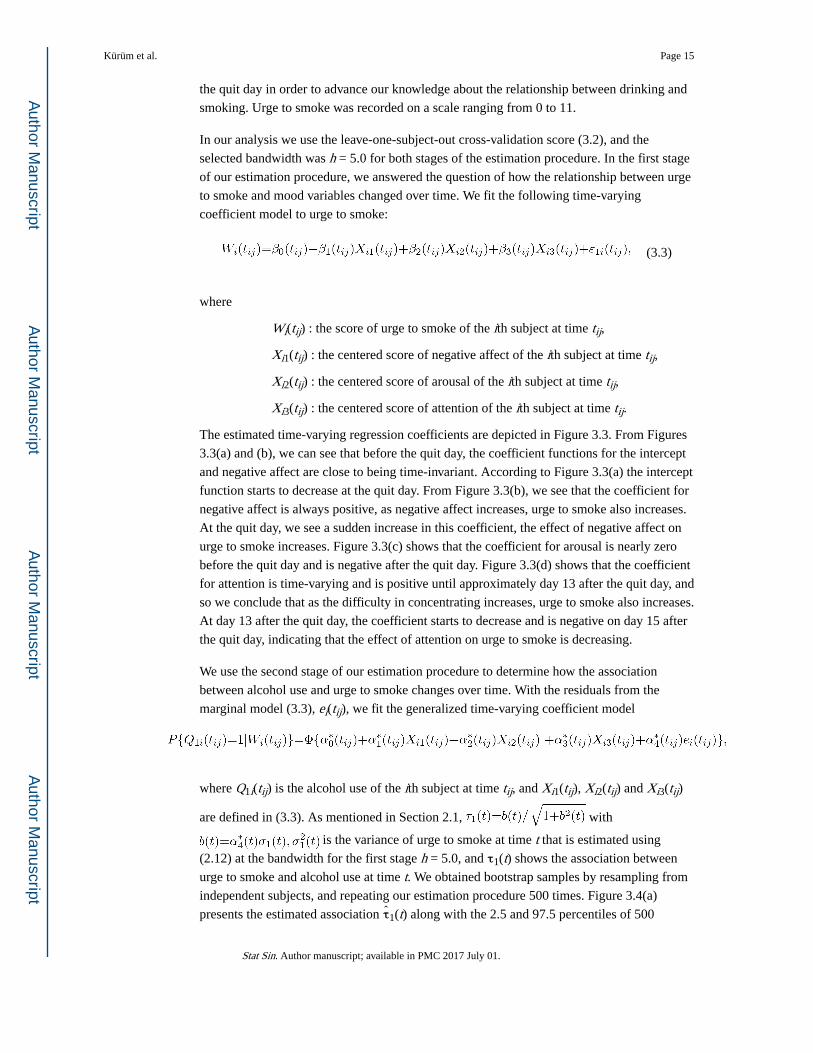
the quit day in order to advance our knowledge about the relationship between drinking and
smoking. Urge to smoke was recorded on a scale ranging from 0 to 11.
In our analysis we use the leave-one-subject-out cross-validation score (3.2), and the
selected bandwidth was h = 5.0 for both stages of the estimation procedure. In the first stage
of our estimation procedure, we answered the question of how the relationship between urge
to smoke and mood variables changed over time. We fit the following time-varying
coefficient model to urge to smoke:
(3.3)
where
Wi(tij) : the score of urge to smoke of the ith subject at time tij,
Xi1(tij) : the centered score of negative affect of the ith subject at time tij,
Xi2(tij) : the centered score of arousal of the ith subject at time tij,
Xi3(tij) : the centered score of attention of the ith subject at time tij.
The estimated time-varying regression coefficients are depicted in Figure 3.3. From Figures
3.3(a) and (b), we can see that before the quit day, the coefficient functions for the intercept
and negative affect are close to being time-invariant. According to Figure 3.3(a) the intercept
function starts to decrease at the quit day. From Figure 3.3(b), we see that the coefficient for
negative affect is always positive, as negative affect increases, urge to smoke also increases.
At the quit day, we see a sudden increase in this coefficient, the effect of negative affect on
urge to smoke increases. Figure 3.3(c) shows that the coefficient for arousal is nearly zero
before the quit day and is negative after the quit day. Figure 3.3(d) shows that the coefficient
for attention is time-varying and is positive until approximately day 13 after the quit day, and
so we conclude that as the difficulty in concentrating increases, urge to smoke also increases.
At day 13 after the quit day, the coefficient starts to decrease and is negative on day 15 after
the quit day, indicating that the effect of attention on urge to smoke is decreasing.
We use the second stage of our estimation procedure to determine how the association
between alcohol use and urge to smoke changes over time. With the residuals from the
marginal model (3.3), ei(tij), we fit the generalized time-varying coefficient model
where Q1i(tij) is the alcohol use of the ith subject at time tij, and Xi1(tij), Xi2(tij) and Xi3(tij)
are defined in (3.3). As mentioned in Section 2.1, with
is the variance of urge to smoke at time t that is estimated using
(2.12) at the bandwidth for the first stage h = 5.0, and τ1(t) shows the association between
urge to smoke and alcohol use at time t. We obtained bootstrap samples by resampling from
independent subjects, and repeating our estimation procedure 500 times. Figure 3.4(a)
presents the estimated association τ̂1(t) along with the 2.5 and 97.5 percentiles of 500
Kürüm et al. Page 15
Stat Sin. Author manuscript; available in PMC 2017 July 01.
Author M
anuscriptA
uthor Manuscript
Author M
anuscriptA
uthor Manuscript

bootstrap samples. According to Figure 3.4(a) before the quit day, urge to smoke and alcohol
use have a positive relationship but after the quit day the relationship is negative. In other
words, before the quit day increased urge to smoke is associated with alcohol usage, whereas
after the quit day reduced urge to smoke is associated with alcohol usage. Based on the
relationship between τ1(t) and , we investigated the significance of the association
using the confidence intervals for . Figure 3.4(b) depicts the estimated regression
coefficient along with its confidence intervals. Figure 3.4(b) demonstrates that the
association between alcohol use and urge to smoke is time-varying, is significant before the
quit day but insignificant after the quit day. This may be due to lack of enough data.
Also of interest is the association between urge to smoke and the presence of other smokers.
Shiffman and Balabanis (1995), McDermut and Haaga (1998) and Warren and McDonough
(1999) observed that the sight of other smokers tends to provoke a craving to smoke. By
employing our joint modeling technique, we studied how this association changes over time.
In this analysis, the selected bandwidth was h = 5.0 for both stages. First we fit the time-
varying coefficient model to urge to smoke; the model is the same as the one in the alcohol
usage analysis (3.3). We observed the same trends in the regression coefficients as in Figure
3.3, since the only difference between these two analyses is that we removed subjects with
missing values for this binary response. The plots are omitted.
In the second stage of our estimation procedure, we used the residuals from the marginal
model (3.3) and fit the generalized time-varying coefficient model
where Q2i(tij) is the response of the ith subject at time tij on presence of other smokers, and
Xi1(tij), Xi2(tij), and Xi3(tij) are defined in (3.3). Here with
, and τ2(t) shows the association between urge to smoke and presence of
other smokers at time t. Similar to our analysis for estimating τ1(t), we estimated σ1(t) using
(2.12) at the bandwidth for the first stage h = 5.0. Figure 3.4(c) demonstrates the estimated
association τ̂2(t) along with 2.5 and 97.5 percentiles of 500 bootstrap samples. Figure 3.4(c)
indicates that the association between the presence of other smokers and urge to smoke is
almost always positive. In other words, the presence of other smokers is always associated
with an increased urge to smoke. As indicated by the relationship between τ2(t) and ,
we can investigate the significance of the association using the confidence intervals for
. Figure 3.4(d) shows the estimated regression coefficient along with its
confidence intervals. According to Figure 3.4(d) the relationship between urge to smoke and
presence of other smokers is time-invariant and significant until around day 13 after the quit
day. After this day, it appears to be insignificant perhaps due to not having a sufficient
number of observations.
Kürüm et al. Page 16
Stat Sin. Author manuscript; available in PMC 2017 July 01.
Author M
anuscriptA
uthor Manuscript
Author M
anuscriptA
uthor Manuscript

4. Discussion
We have proposed a joint modeling methodology for estimating the time-varying association
between longitudinal binary and continuous responses. We developed a two-stage estimation
procedure based on local linear regression, and derived standard error formulas for our
estimators in both stages. A simulation study showed that our procedure works well on
estimating both the time-varying relationship between longitudinal binary and continuous
responses and the true standard errors of the estimators. We applied our method to a dataset
of lapsed participants in a smoking cessation study and gained insight regarding two
relationships: urge to smoke and alcohol use, and urge to smoke and presence of other
smokers.
We are aware that in practice an association between the binary and continuous responses
measured at different time points may exist; however, we did not model this association and
showed in Section 2.3 that it does not affect the asymptotic behavior of the proposed
estimates in either stages of the estimation procedure.
Supplementary Material
Refer to Web version on PubMed Central for supplementary material.
Acknowledgments
The authors are grateful to the Editor, an associate editor and the referees for valuable comments that significantly improved the paper. Li’s research was supported by National Institute on Drug Abuse/National Institute of Health grants P50-DA10075 and P50 DA039838, National Cancer Institute grant R01 CA168676, and National Science Foundation grant DMS-1512422. Yao’s research is supported by National Science Foundation grant DMS-1461677. The content is solely the responsibility of the authors and does not necessarily represent the official views of these organizations.
References
Brumback BA, Rice JA. Smoothing spline models for the analysis of nested and crossed samples of curves. Journal of American Statistical Association. 1998; 93:961–976.
Cai Z, Fan J, Li R. Efficient estimation and inferences for varying-coefficient models. Journal of the American Statistical Association. 2000; 95:888–902.
Catalano PJ, Ryan LM. Bivariate latent variable models for clustered discrete and continuous outcomes. Journal of the American Statistical Association. 1992; 87:651–658.
Cox DR, Wermuth N. Response models for mixed binary and quantitative variables. Biometrika. 1992; 79:441–461.
Dunson DB. Bayesian latent variable models for clustered mixed outcomes. Journal of the Royal Statistical Society B. 2000; 62:355–366.
Fan, J.; Gijbels, I. Local Polynomial Modelling and Its Applications. London: Chapman and Hall; 1996.
Fan J, Huang T, Li R. Analysis of longitudinal data with semiparametric estimation of covariance function. Journal of American Statistical Association. 2007; 102:632–641.
Fitzmaurice GM, Laird NM. Regression models for a bivariate discrete and continuous outcome with clustering. Journal of the American Statistical Association. 1995; 90:845–852.
Gueorguieva R. A multivariate generalized linear mixed model for joint modelling of clustered outcomes in the exponential family. Statistical Modelling: An International Journal. 2001; 1:177–193.
Kürüm et al. Page 17
Stat Sin. Author manuscript; available in PMC 2017 July 01.
Author M
anuscriptA
uthor Manuscript
Author M
anuscriptA
uthor Manuscript

Gueorguieva RV, Agresti A. A correlated probit model for joint modeling of clustered binary and continuous responses. Journal of the American Statistical Association. 2001; 96:1102–1112.
Hastie T, Tibshirani R. Varying-coefficient models. Journal of the Royal Statistical Society B. 1993; 55:757–796.
Hodges J, Reich B. Adding spatially-correlated errors can mess up the fixed effect you love. The American Statistician. 2010; 64:325–334.
Hoover DR, Rice JA, Wu CO, Yang L-P. Nonparametric smoothing estimates of time-varying coefficient models with longitudinal data. Biometrika. 1998; 85:809–822.
Hymowitz N, Cummings KM, Hyland A, Lynn WR, Pechacek TF, Hartwell TD. Predictors of smoking cessation in a cohort of adult smokers followed for five years. Tobacco Control. 1997; 6:S57–S62. [PubMed: 9583654]
Kahler CW, Spillane NS, Metrik J. Alcohol use and initial smoking lapses among heavy drinkers in smoking cessation treatment. Nicotine & Tobacco Research. 2010; 12:781–785. [PubMed: 20507898]
Liu X, Daniels M, Marcus B. Joint models for the association of longitudinal binary and continuous processes with application to a smoking cessation trial. Journal of the American Statistical Association. 2009; 104:429–438. [PubMed: 20161053]
McDermut W, Haaga DA. Effect of stage of change on cue reactivity in continuing smokers. Experimental and Clinical Psychopharmacology. 1998; 6:316–324. [PubMed: 9725115]
Regan MM, Catalano PJ. Likelihood models for clustered binary and continuous outcomes: Application to developmental toxicology. Biometrics. 1999; 55:760–768. [PubMed: 11315004]
Roy J, Lin X. Latent variable models for longitudinal data with multiple continuous outcomes. Biometrics. 2000; 56:1047–1054. [PubMed: 11129460]
Sammel MD, Ryan LM, Legler JM. Latent variable models for mixed discrete and continuous outcomes. Journal of the Royal Statistical Society B. 1997; 59:667–678.
Shiffman, S.; Balabanis, M. Associations between alcohol and tobacco. In: Fertig, JB.; Allen, JP., editors. Alcohol and Tobacco: From Basic Science to Clinical Practice. Bethesda, MD: National Institutes of Health; 1995. p. 17-36.
Shiffman S, Balabanis MH, Gwaltney CJ, Paty JA, Gnys M, Kassel JD, Hickcox M, Paton SM. Prediction of lapse from associations between smoking and situational antecedents assessed by ecological momentary assessment. Drug and Alcohol Dependence. 2007; 91:159–168. [PubMed: 17628353]
Shiffman S, Gwaltney CJ, Balabanis MH, Liu KS, Paty JA, Kassel JD, Hickcox M, Gnys M. Immediate antecedents of cigarette smoking: An analysis from ecological momentary assessment. Journal of Abnormal Psychology. 2002; 111:531–545. [PubMed: 12428767]
Shiffman S, Hickcox M, Paty JA, Gnys M, Kassel JD, Richards TJ. Progression from a smoking lapse to relapse: Prediction from abstinence violation effects, nicotine dependence, and lapse characteristics. Journal of Consulting and Clinical Psychology. 1996; 64:993–1002. [PubMed: 8916628]
Verbeke, G.; Molenberghs, G.; Rizopoulos, D. Random effects models for longitudinal data. In: van Montfort, K.; Oud, J.; Satorra, A., editors. Longitudinal Research with Latent Variables. Berlin: Springer-Verlag; 2010. p. 37-96.
Warren CA, McDonough BE. Event-related brain potentials as indicators of smoking cue-reactivity. Clinical Neurophysiology. 1999; 110:1570–1584. [PubMed: 10479024]
Wu CO, Chiang C-T, Hoover DR. Asymptotic confidence regions for kernel smoothing of a varying-coefficient model with longitudinal data. Journal of the American Statistical Association. 1998; 93:1388–1402.
Yao W, Li R. New local estimation procedure for nonparametric regression function of longitudinal data. Journal of the Royal Statistical Society B. 2013; 75:123–138.
Zhang W, Lee S-Y. Variable bandwidth selection in varying-coefficient models. Journal of Multivariate Analysis. 2000; 74:116–134.
Kürüm et al. Page 18
Stat Sin. Author manuscript; available in PMC 2017 July 01.
Author M
anuscriptA
uthor Manuscript
Author M
anuscriptA
uthor Manuscript

Figure 3.1. Estimated varying coefficient functions (dashed) of the time-varying coefficient model fit to
the continuous response overlaying the true coefficient functions (solid) along with the
empirical (dotted) and the mean theoretical (dashed-dotted) pointwise 95% confidence bands
based on 500 Monte Carlo replications.
Kürüm et al. Page 19
Stat Sin. Author manuscript; available in PMC 2017 July 01.
Author M
anuscriptA
uthor Manuscript
Author M
anuscriptA
uthor Manuscript

Figure 3.2. Estimated correlation coefficient function (dashed) overlaying the true correlation function
(solid) along with the 2.5 and 97.5 percentiles based on 500 Monte Carlo runs (dotted).
Kürüm et al. Page 20
Stat Sin. Author manuscript; available in PMC 2017 July 01.
Author M
anuscriptA
uthor Manuscript
Author M
anuscriptA
uthor Manuscript

Figure 3.3. Plots of estimated coefficient functions (solid) of the time-varying coefficient model fit to
urge to smoke response along with the 95% pointwise asymptotic confidence intervals
before and after quitting smoking (dashed). We aligned the data so that all subjects have quit
day at day zero. (a) Intercept function, (b) negative affect, (c) arousal, and (d) attention.
Kürüm et al. Page 21
Stat Sin. Author manuscript; available in PMC 2017 July 01.
Author M
anuscriptA
uthor Manuscript
Author M
anuscriptA
uthor Manuscript

Figure 3.4. Estimated time-varying associations along with 2.5 and 97.5 percentiles of 500 bootstrap
samples (a) alcohol versus urge to smoke and (c) presence of other smokers versus urge to
smoke. Estimated coefficient functions (solid) of the generalized time-varying coefficient
model fit along with the 95% pointwise asymptotic confidence intervals (dashed) (b) alcohol
use analysis and (d) presence of other smokers analysis.
Kürüm et al. Page 22
Stat Sin. Author manuscript; available in PMC 2017 July 01.
Author M
anuscriptA
uthor Manuscript
Author M
anuscriptA
uthor Manuscript

Author M
anuscriptA
uthor Manuscript
Author M
anuscriptA
uthor Manuscript
Kürüm et al. Page 23
Tab
le 3
.1
Sum
mar
y of
sim
ulat
ion
resu
lts f
or th
e fi
rst s
tage
h
RA
SE
t
β̂ 1(t)
β̂ 2(t)
Mea
n(SD
)SD
SE (
SDse
)SD
SE (
SDse
)
.30
.051
.049
(.0
05)
.049
.049
(.0
05)
.10
.078
(.0
16)
.50
.042
.037
(.0
03)
.038
.037
(.0
03)
.70
.054
.049
(.0
04)
.051
.049
(.0
05)
.30
.035
.034
(.0
02)
.035
.034
(.0
03)
.20
.062
(.0
14)
.50
.032
.028
(.0
02)
.028
.028
(.0
02)
.70
.038
.034
(.0
02)
.033
.033
(.0
03)
.30
.025
.024
(.0
01)
.023
.023
(.0
02)
.40
.072
(.0
14)
.50
.022
.022
(.0
01)
.022
.022
(.0
01)
.70
.026
.024
(.0
01)
.023
.023
(.0
02)
Stat Sin. Author manuscript; available in PMC 2017 July 01.

Author M
anuscriptA
uthor Manuscript
Author M
anuscriptA
uthor Manuscript
Kürüm et al. Page 24
Tab
le 3
.2
Sum
mar
y of
sim
ulat
ion
resu
lts f
or th
e se
cond
sta
ge
h
RA
SE
t
Mea
n(SD
)SD
SE (
SDse
)SD
SE (
SDse
)SD
SE (
SDse
)
.30
.069
.066
(.00
2).0
68.0
66(.
003)
.071
.071
(.00
5)
.10
.080
(.02
0).5
0.0
73.0
69(.
002)
.077
.074
(.00
5).1
00.0
95(.
007)
.70
.070
.066
(.00
2).0
67.0
66(.
003)
.077
.071
(.00
5)
.30
.048
.046
(.00
1).0
47.0
47(.
002)
.056
.052
(.00
3)
.20
.052
(.01
9).5
0.0
48.0
48(.
001)
.052
.050
(.00
2).0
64.0
60(.
004)
.70
.048
.046
(.00
1).0
46.0
46(.
002)
.057
.053
(.00
3)
.30
.035
.034
(.00
1).0
35.0
34(.
001)
.043
.041
(.00
2)
.40
.064
(.02
0).5
0.0
34.0
33(.
001)
.034
.033
(.00
1).0
41.0
37(.
002)
.70
.034
.034
(.00
1).0
34.0
34(.
001)
.044
.041
(.00
2)
Stat Sin. Author manuscript; available in PMC 2017 July 01.