International Journal of Water Resources and Environmental Engineering Vol. 3(x), pp. xx-xx, September 2011 Available online at http://www.academicjournals.org/ijwree ISSN 1991-637X © 2011 Academic Journals

Full Length Research Paper

Time series analysis of ground water table fluctuations due to temperature and rainfall change in Shiraz plain

Mohamad Aflatooni1* and Mehdi Mardaneh2

1Assistant professor, Islamic Azad Universirty, Shiraz Branch, Department of Water Resources, Shiraz, Iran.

2Department of Agriculture, Marvdasht Branch, Islamic Azad University, Marvdasht, Iran.

Accepted 10 August, 2011

This research aims at forecasting ground water fluctuations due to temperature and rainfall effects using time series and cross-correlation analysis. Box Jenkins’s time series model was analyzed and the

best one for Shiraz plain proved to be multiplicative seasonal 12210212 ),,(),,( ×ARIMA . This model was

used to forecast the future ground water fluctuations as affected by long term temperature and rainfall data. Results showed that the average annual water table elevation was 1499.31 for year 2021. The elevation for the year 2007 was 1501.03 showing 1.72 meter decline. Among 29 wells, statistical analysis showed that 89% of the wells had a negative correlation with monthly temperature but 86% of them showed a positive correlation with monthly rainfall. A cross-correlation analysis using individual wells showed 44.8% of wells had a delay time due to temperature changes between zero to 2 months, 51% between 10 to 14 months and only 3.5% of 26 months. Also, 72.4% of wells had a response time due to rainfall of zero to 2 months, 24.1% between 11 to 23 months and the response of 3.5% was 38 months. On average, the delay time of water table fluctuation due to temperature changes for Shiraz plain was 13 months and due to rainfall was 1 month. Key Words: Box Jenkings model, temperature, rainfall, cross-correlation, water table level, plain, correlation, time delay, change, multiplicative seasonal model.

INTRODUCTION Water resources in any part of the world are subject to change due to meteorological and climatological impact all the year long. Impact of these factors on water resources has been extensively studied (Chen and Osadetz, 2002; Gleick, 1989; Maathuis and Thorleeifson, 2000; Lewis, 1989). Increased temperature, plant water requirements, demand for human and animal drinking water and industrial usage, limited rainfall on one hand and artificial ground water recharge on the other hand, requires more water resource development and planning activities in the future. Dealing with variations of ground water resources in relation to effect of rainfall and temperature on water table fluctuations is an important factor which plays a media role in sustainable ground water development. Physical relationships between *Corresponding author. E-mail:moh01012500@yahoo.com. Tel: 0711-6254621.

meteorological factors, unsaturated and saturated zones of phreatic ground water resources, as is the case in the region's conditions, is cited elsewhere (Aflatooni, 2011). The long term historical and meteorological data ,among all, temperature and rainfall can be used to assess the future surface water, ground water table and storage variations in order to have a better insight into the problem posed in the future. In general, if the statistical parameters such as mean and variance of a long term meteorological time series changes steadily, it can be said that the climate change is inevitable, so using these historical times series and their effects on water resources ,mainly ground water, may have a similar future impact. Analysis of time series as related to ground water table seeks two objectives; modeling of random variables to have an understanding of historical data and forecasting future data behavior based on the past data(Ahn, 2000). We should understand the significant statistical characteristics between meteorogical data and those of say ground water table variations separating

them into deterministic components or the ones that can be modeled. A time series, apart from a modeling component has a random component which cannot be modeled. On this basis, a suitable model must have the ability of modeling all deterministic components(Yevjevich, 1982). In Iran, research solely concerning effects of climatic variables on ground water table hydrograph as predicted by time series analysis is scarce (Mardaneh and Aflatooni, 2009). However, scattered researches on various aspects in this country such as; study of time series on water resources (Mirsaii et al, 2006), study of climate change using time series(Tabatabai and Hosseini, 2002), using stochastic methods to study ground water level (Rahmani, 2004), stochastic behaviour of river flows(Samani et al, 1994; Sedghi, 2000) and reservoirs(Jalali, 1983) may be cited. Extensive usage of time series and/or stochastic modeling of water level fluctuations are cited in the litreture(Chow, 1978; Chow and Kareliotis, 1970; Salas, 1997). In this research, Box-Jenkings time series method(Pankratz, 1983) was used to predict and possibly forecast the future ground water table fluctuations. Box-Jenkings method was used because it takes into account all behaviors of the water table time series including randomness, seasonality, periodicity and stationarity. Also, a cross correlation analysis between ground water table elevations and temperature/rainfall data was conducted to forecast present and future impacts of these two parameters on ground water behavior and its time delay in Shiraz plain, Fars province, Iran. MATERIALS AND METHODS Theory Box-Jenkings is a type of stationary time series model in the form of

),)(,( QPqpARIMA where qp , are non-seasonal and

QP , are seasonal order of auto-regressive and moving average

processes, respectively. Introducing two differential coefficients

Dd , to this form to overcome the problem of trend, seasonality

and non-stationarity, the model is corrected and written in the form

of sQDPqdpARIMA ),,)(,,( where Dd , are respectively

the degree of simple and seasonal differentiation which comes up to less than or equal to unity. In general, to show the capability of a mathematical or statistical model, we have to perform three basic procedures, namely; identification of parameters, fitting the model in observed data and validation of the model in order to be able to use it for predictive or forecasting purposes. The general Box-Jenkings model is written as follows (Pankratz, 1983):

t

s

Qqt

dD

s

s

Pp ZBBXBB )()()()( θθθφφ +=∇∇o

(1)

Where, (1) )()( p

pp BBBB φφφφ −−−−= L2

211 is

a no seasonal autoregressive operator of order p

(2) )()( ,,

Ps

sP

s

s

s

P BBB φφφ −−−= L11 Is a

seasonal autoregressive operator of order P .

(3) )1()( 2

21

q

qq BBBB θθθθ −−−−= L Is a no

seasonal moving average operator of order? q

(4) )()( ,,

Qs

sQ

s

s

s

Q BBB θθθ −−−= L11 Is seasonal

moving average operator of order Q .

(5) )()(s

Pp BB φµφθ =o

Is the model constant where µ is

the real mean of the stationary time series being modeled?

(6) ,..., 1−tt ZZ Are the random noise terms having normal

distribution? (7)

sQssqsPssp ,,2,121,,2,121 ,..,,,,...,,,...,,,,...,, θθθθθθφφφφφφ An

d σ are unknown coefficients which are about to be determined

using observed data.

(8) B is a backward operator in the form of ktt

kXXB −=

(9) ∇ is a non-seasonal operator defined as B−=∇ 1 and

s∇ is a seasonal operator defined as s

sB−=∇ 1

Given the observed piezometer (water well) data, the initial statistical analysis consisted of removing the outliers, test of normal distribution, using ACF

1 and PACF

2 to determine the correlation of

model components and computation of coefficients, removing trend and seasonality from time series, determination of seasonal index, statistical test of time length of data and converting non-stationarity to stationary state. Calculation of seasonal index for each month was done by multiplicative method as shown in Figure 3 Finally, the selected model coefficients were so calibrated that the statistical

criteria such as AICMEMAPEMAERMSE ,,,, be the

least. The selected model was then validated using one fifth of data length from the end of the data record. After model validation, it was used to forecast the ground water table in future periods.

cStatgraphiandSPSS. Software was appropriately used for

all the computations. Since we are concerned with the correlation with a delayed time situation (that is, water table fluctuates with a time delay due to a change in temperature and rainfall), we then used the cross correlation analysis to determine the effect of these two parameters on ground water table fluctuations. The following formulas were used in the analysis (Rutulis, 1989):

∑ =−−=−

=+

kN

tkttxy kforyyxx

NC

1

,...2,1,0))((1

(2)

,...2,1,0))((1

1

−−=−−∑= +

+

=

kforxxyyN

C kt

kN

ttxy

(3)

yx

xy

xy

kCkr

σσ

)()( =

(4)

1 -Auto-regressive correlation function

2 -partial auto-regressive correlation function

)(,)( oo yyyxxx CC == σσ

(5)

Where, N is the number of observations, k is the time lag in

relation to cross correlation )1( −≤ Nk , )(kC xy is cross-

correlation factor for given time lag, )(krxy

is coefficient of cross-

correlation, tx is either temperature or rainfall variable, ty is the

water table elevation variable and yx σσ , are the standard

variations of the above-mentioned time series. It worth noting that Equation 2 is used to compute cross correlation of temperature-

water table or rainfall-water table for forward lag ( 0>k ).

Likewise, Equation 3 is used to compute cross correlation of temperature-water table or rainfall-water table for backward lag

( 0<k ).

Response of ground water to temperature and rainfall changes has a time delay, that is, when it rains or temperature increases, the water table response occurs at a later time known as time delay. In fact, water deficit builds up in unsaturated or root zone due to evapotranspiration, but this deficit is removed or decreased due to rainfall. Since building up and decrease of the deficit may take some time, thus, water table occurs with a time delay in response to temperature and rainfall accordingly. Theoretically, this time delay is usually difficult to determine but using cross-correlation analysis, we are able to estimate it. Time delay is defined when two time series reach the maximum correlation (Rutulis, 1989):

))()...1(()(: NrrMaxtriftt xyxyxy ==∆

(6) Also, following relations are used in the analysis (Rutulis, 1989):

τbav +=

(7)

Tw /))(sin( ωτπβα −+= 2

(8)

[ ]2

1

)(∑=

+−=N

t

wvx τττψ

(9) Where equation (7) is non linear model containing a linear trend. Equation (8) is a periodic long term function used to indicate the climate variations. Equation (9) is an objective function used to

determine the unknown parameters βα ,,,ba when ψ is

minimized. τ is time in month, ω,T are phase and periodic

length respectively. τx is observed temperature or rainfall and

ττ wv + is computed data using Equations 7 and 8, respectively.

Thus, the response time of ground water level to temperature and

rainfall ( t∆ ) can be determined using maximum coefficient of

correlation between two variables (water table-temperature or water table-rainfall) was determined. These computations were done

using SPSS software.

Case study location

The study was conducted in Maharloo basin located in south west

of Iran (Figure 1a). Having an area of24270 km , the basin is

located in 630129 ′−′ oo northern latitude and

82532152 ′−′ oo eastern longitude. Shiraz plain is part of the

basin having an area of 2230 km where the research was

conducted (Figure 1a). Spatial distribution of water wells (a total of 29) is given in Figure 1b where the wells are numbered 1 through 29 along with their UTM coordinates. Monthly temperature and rainfall data were obtained from a synoptic meteorological station near the plain. Monthly temperature, rainfall and water table data are all from 1993 to 2007.

RESULTS AND DISCUSSION Statistics calculated for ground water level time series are given in Table 1. Monthly and yearly trend of this time series is shown in Figure 2a and 2b respectively. Apart from the trend in monthly time series, it has also a seasonal variation. Comparison of seasonal index of observed and predicted ground water level time series for each month is given in table 3 The highest seasonal index (100.07%) is for month 12 (February 20 to March 19), therefore for the period of 175

3 months with

1501.35m ground water elevation, the maximum

elevation was m4.150235.15010007.1 =× . Month 7

(September 23 to October 23), had the least ground water elevation in the same period (1500.36 m) due to least ground water elevation of 1500.36 and a seasonal

index of 99.934% ( )36.150099934.036.1500 m=× .

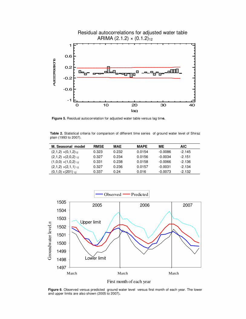
Other seasonal indices vary between the minimum and the maximum month, so the ground water level time series for the period of 175 months had seasonal variation with a period equal to 12 months. This indicates that the time series has a trend and seasonality; it thus is non-stationary and should be converted to stationary state to be used in Box-Jenkings model. Figure 4 shows the auto-correlation function (ACF) and partial autocorrelation function (PACF) of the time series; ACF like a declining wave tends to decrease and PACF, after lag 1, changes non-uniformly. Autocorrelation of residuals for adjusted water table levels (ACF of residuals) is also shown in Figure 5. Statistical criteria for comparison among the multiplicative seasonal models are shown in Table 2. This Figure shows that the residuals cross the confidence interval at the least lag time. This Table and the ACF and PACF diagrams show that the best model of this type fitted in ground water time series is

12)2,1,0()2,1,2( ×ARIMA , where number 12 indicates

the seasonality parameter( s ) in corrected Box-Jenkings

model given by SQDPqdpARIMA ),,)(,,( , and

2,1,0,2,1,2 ====== QDPqdp indicate

the rank parameters of the model. In Table 2, the

3 - Monthly available data

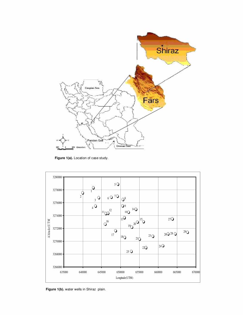
Figure 1(a). Location of case study.

3266000

3268000

3270000

3272000

3274000

3276000

3278000

3280000

635000 640000 645000 650000 655000 660000 665000 670000

Longitude(UTM)

Alt

itu

de(

UT

M)

2

1

3

5

4

67

8

9

101112

13

14

1516

1718

1920

21

22

23

24

25

26

27

2829

Figure 1(b). water wells in Shiraz plain.

Table 1.Statistics for mean monyhly ground water level time series of Shiraz plain (1993 to 2007).

No. of Months Min. Max. Range SD Average Slope of trend line Correlation

175 1498.44 1504.14 5.69 1.2 1501.35 -0.0141 +0.3

y = -0.0141x + 1502.6

R2 = 0.3013

1498

1499

1500

1501

1502

1503

1504

1505

Marc

h

Marc

h

Marc

h

Marc

h

Marc

h

Marc

h

Marc

h

Marc

h

Marc

h

Marc

h

Marc

h

Marc

h

Marc

h

Marc

h

Marc

h

First month of each year

Wate

r ta

bl(

m)

1993 1994 1995 1996 1997 1998 1999 2000 2001 2002 2003 2004 2005 2006 07

(a)

Figure 2(a). Mean yearly ground water table elevations in shiraz plain (1993-2007). Vertical ordinate is ground water elevation, m.

y = -0.1715x + 1844.3

R2 = 0.473

1499.50

1500.00

1500.50

1501.00

1501.50

1502.00

1502.50

1503.00

1503.50

1991 1993 1995 1997 1999 2001 2003 2005 2007

Year

Wate

r ta

ble

(m)

y=0.1715x + 1844.3 R

2=0.473

(b)

Figure 2(b). Trend of ground water table elevations in shiraz plain (1993-2007). Vertical ordinate is ground water elevation, m.

minimum statistical comparison criteria RMSE, MAE and MAPE, among all, indicate that the best fit

is 12)2,1,0()2,1,2( ×ARIMA . The constant value 00 =θ

and the white noise (or the variance of exact random

series) is equal to 11564.02 =σ . Thus the exact

random time series is given as:

)115647.0,0(),( 2 WnWnZ t == σµ (10)

equal to model coefficients (Equation 12) as follows:

1661787.0)2(;681855.0)1(

976364.0)2(;102608.0)1(

967394.0)2(;05473.2)1(

12,212,1

21

21

====

−==−==

−==−==

θθ

θθ

φφ

SMASMA

MAMA

ARAR

Since 0=P , no coefficient is calculated for it. Finally the

multiplicative seasonal model for ground water time series is given as:

Figure 3. Variation of seasonal index of ground water level, % (1993 to 2007).

t

s

Qqt

dD

s

s

Pps ZBBXBBQDPqdpARIMA )()()()(:),,(),,( θθθφφ +=∇∇×o

(11) which comes to:

tt ZBBXBBARIMA )()())(()2,1,0()2,1,2(12

22

11

12

12

212 θθφ =∇∇≡×

(12)

Where tZ is given in equation (10). Figure 6 shows

mean monthly observed and predicted ground water levels as calculated by equation (12) versus first month of each year for the period 1993 to 2007. The lower and upper limits of ground water levels with 95% confidence interval are also shown in the Figure. The Statgraphics software was used for the calculations. This Figure shows there is a decline and rise of water table elevations for the entire period and the model compares well with observations with the highest level in the month 7. The scatter diagram of observed versus predicted water table level is given in Figure 7. The slope of the line when the intercept is zero is equal to 1.0006 and when it is nonzero is equal to 0.8366, in both cases the slope is assumed to be nearly equal to unity. This diagram shows reasonable agreement between observed and predicted water table elevations for validation period 2005 to 2007. Figures 8a and 8b show average monthly and yearly trend of forecasted ground water level in Shiraz plain for period 2007 to 2021. Theissen polygon was used to calculate the weighted average values of water table levels in the plain. It is seen that the water table fluctuated between 1499.31 to 1501.32 and the water table for the year 2021 is 1499.31 meter from the sea level with 95% confidence. Therefore, the decline of water table is about 1.72 m for this period. The average water table level for the forecasted period (2007 to 2021) is 1500.54 m while the average value for predicted period (1993 to 2007) is 1501.35 which shows 0.81 m

decline in future. By predicted period, we mean the period we had water table observations data. Tests showed that having 175 months (observation period) of water table data, the predictions for this time period were possible (Figure 2a and 2b) and forecast for the second 175 months (forecasting or projecting period) is also possible (Figure 8a and 8b). Beyond second 175 months(long term projecting period), however, the predictions got closer to mean water table level as the time went on and finally displaying a straight line(data not shown). Comparison of the seasonal index for 1993 to 2007 time period shows that month 12 with highest index has the highest and month 7 with the lowest index has the lowest ground water level (Figure 9 and Table 3). Apart from the mean monthly water level analysis averaged over the plain, data of individual wells were also analyzed. The graph of water table level versus time for 29 wells showed that 90 % of the wells had a declining trend (negative trend slope) and will have the problem of water level decrease in the future provided that the water consumption in future be the same as the past (Table 4). However, contrary to our assumption, the water consumption (agricultural, municipal, residential, commercial and the like) in future can vary so that it clearly affects the trend of the declining lines. Monthly temperature and ground water table of individual wells for the years 1993 to 2007 and monthly rainfall and ground water table were correlated for the same period (Table 4). A negative correlation coefficient (-0.1982) between temperature and the water table level in about 89% of the wells was shown while the coefficient between rainfall and ground water level was positive(+0.1294) in 86% of wells. The analysis of correlation shows that in majority of cases any change in temperature or rainfall will influence the water table level

3

6

3

5

3

4

3

3

3

2

3

1

3

0

2

9

2

8

2

7

2

6

2

5

2

4

2

3

2

2

2

1

2

0

1

9

1

8

1

7

1

6

1

5

1

4

1

3

1

2

1

1

1

0

987654321

Lag number

1.0

0.5

0.0

-0.5

-1.0

ACF

Lower confidencelimit

Upper confidence l

Coefficient

Watertable

(a)

3 6

3 5 3

4 33

32

3 1 3

0 29

28

27 2

6 2 5

24 2

3 2 2 2

120

1 9

1 8 1

716

1 5 1

413

12

11

1 0 9876 5 4 321

Lag number

1.0

0.5

0.0

-0.5

-1.0

Part

ial A

CF

Lower confidence

limit

Upper confidence Limit

Coefficient

Watertable

b

Figure 4. Autocorrelation functions of ground water level time series; ACF (a) and PACF, (b) versus

lag number (1993 to 2007).

Residual Autocorrelations for adjusted Watertable

ARIMA(2,1,2)x(0,1,2)12

0 10 20 30 40

lag

-1

-0.6

-0.2

0.2

0.6

1

Autocorrelations

Residual autocorrelations for adjusted water table ARIMA (2.1.2) × (0.1.2)12

Figure 5. Residual autocorrelation for adjusted water table versus lag time.

Table 2. Statistical criteria for comparison of different time series of ground water level of Shiraz

plain (1993 to 2007).

M. Seasonal model RMSE MAE MAPE ME AIC

(2,1,2) ×(0,1,2)12 0.323 0.232 0.0154 -0.0086 -2.145

(2,1,2) ×(2,0,2) 12 0.327 0.234 0.0156 -0.0034 -2.151

(1,0,0) ×(1,0,2) 12 0.331 0.238 0.0158 -0.0066 -2.136

(2,1,2) ×(2,1,1) 12 0.327 0.236 0.0157 -0.0031 -2.134

(0,1,0) ×(201) 12 0.337 0.24 0.016 -0.0073 -2.132

1497

1498

1499

1500

1501

1502

1503

1504

1505

March March March

First month of each year

Gro

und

wat

er lev

el.m

Observed Predicted

2005 2006 2007

Upper limit

Lower limit

Figure 6. Observed versus predicted ground water level versus first month of each year. The lower and upper limits are also shown (2005 to 2007).

1497

1498

1499

1500

1501

1502

1503

1504

1505

March March March

First month of each year

Gro

und

wat

er l

evel

.m

Observed Predicted

2005 2006 2007

Upper limit

Lower limit

Figure 7. Observed versus predicted ground water level (2005 to 2007). The lines

have different intercepts as given.

y = -0.0175x + 1500.9

R2 = 0.5149

1496.00

1497.00

1498.00

1499.00

1500.00

1501.00

1502.00

1503.00

Marc

h

Marc

h

Marc

h

Marc

h

Marc

h

Marc

h

Marc

h

Marc

h

Marc

h

Marc

h

Marc

h

Marc

h

Marc

h

Marc

h

Marc

h

First month of each year

Gro

undw

ate

r le

vel,

m

07 08 09 10 11 12 13 14 15 16 17 18 19 20 21

(a)

(b)

Figure 8. Average monthly (a) and yearly (b) trend of ground water level in Shiraz

plain(2007 to 2021).

Figure 9. Comparison of average monthly ground water level trend for 1993 to 2007 measured and 2007-2021 forecast.

Table 3. Comparison of seasonal index (%)of observed and predicted group water level times series for different months of the year (1993 to 2007).

Month Measured water level seasonal index(1993 to 2007) Predicted water level seasonal index, % (2007 to 2021)

1 100.064 100.071

2 100.052 100.056

3 100.022 100.019

4 99.989 99.987

5 99.963 99.959

6 99.939 99.936

7 99.934 99.925

8 99.945 99.943

9 99.968 99.964

10 100.003 100.005

11 100.047 100.055

12 100.047 100.077

accordingly; that is an increase in temperature will decrease water table elevation while an increase in rainfall will increase the water table elevation.

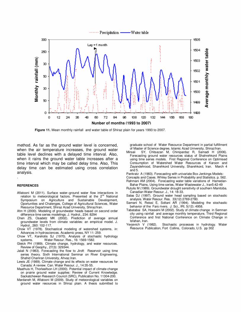
To find out the time delay, a cross correlation analysis was performed. Results of cross correlation between temperature and water level on one hand and rainfall and water table on the other hand for individual wells are given in Tables 5 and 6, respectively. In these cross correlation (C.C.) Tables, time lag or delay and standard deviations (STD) are shown where time lag is in month. The results show that 44.8% of the wells had a time delay of zero to 2 months, 51.7% between 10 to 14 and only 3.5 % of 26 months. On average, the time delay of ground water level in response to temperature is 13 months ignoring the 3.5% case. As far as the rainfall is concerned, 72% of the wells had a time delay of zero to 2

month, 24.1 % between 11 to 23 month and only 3.5% of 38 months. Similarly, on average, the delay of water level response to rainfall is about 1 month. As mentioned earlier, the temperature and rainfall data were chosen since they reflect the major meteorological parameters of the region's climate. In fact, these two parameters mainly affect the water deficit and/or water balance in unsaturated zone and before the net recharge from rainfall reaches ground water storage, the water deficit thus generated by evapotranspiration from the root or unsaturated zone must be satisfied first by rainfall (Aflatooni, 2011). The reason for existence of time delay is, in fact, due to this water deficit. It worth noting there is enough evidence that the temperature plays a major role on ET. Measured ET data for the region, however, were not available for the period of study.

Table 4. Model type, constant values, inclination slope, correlation coefficients of time series model for water wells of Shiraz plain (1993 to 2007).

Well No. M. seasonal model Constant value Inclination slope C.C. ( R2)

1 (0,1,0) × (2,1,2)12 - -0.0120 0.1340

2 (1,1,2) × (2,1,2) 12 - -0.0365 0.5640

3 (1,0,1) × (1,1,2) 12 - -0.0160 0.2410

4 (1,0,0) × (1,1,2) 12 - -0.0276 0.5110

5 (0,1,0) × (1,0,1) 12 - -0.0340 0.2900

6 (1,1,1) × (2,1,2) 12 - -0.0146 0.2870

7 (1,1,1) × (2,0,1) 12 - -0.0097 0.1800

8 (1,1,1) × (2,0,1) 12 - -0.0189 0.3900

9 (2,0,0) × (2,1,2) 12 -0.21459 -0.0140 0.4420

10 (1,1,2) × (2,0,2) 12 +0.00015 -0.0120 0.3200

11 (1,1,1) × (2,1,2) 12 - -0.0130 0.3450

12 (1,0,1) × (2,1,2) 12 -0.029 -0.0155 0.4480

13 (0,1,2) × (0,1,1) 12 - -0.0207 0.4370

14 (1,0,0) × (2,0,1) 12 -22.386 -0.0074 0.0860

15 (2,0,0) × (2,1,2) 12 -0.1357 -0.0170 0.2900

16 (1,0,0) × (1,0,1) 12 -43.324 +0.0017 0.0050

17 (2,1,2) × (2,1,2) 12 - -0.0090 0.0870

18 (1,0,2) × (2,1,2) 12 -0.0146 -0.0123 0.1470

19 (1,0,2) × (2,1,2) 12 -0.1239 -0.0068 0.0460

20 (1,1,1) × (2,1,2) 12 - -0.0153 0.2260

21 (2,0,0) × (2,1,2) 12 -0.03299 -0.0083 0.2740

22 (1,0,1) × (2,1,2) 12 -89.3179 +0.0035 0.0030

23 (1,1,1) × (2,0,2) 12 - -0.0096 0.1230

24 (1,0,0) × (1,0,2) 12 -31.2447 -0.0140 0.4680

25 (1,0,2) × (1,1,2) 12 - -0.0082 0.0450

26 (0,1,0) × (2,1,0)12 - -0.0485 0.6800

27 (1,0,0) × (0,1,1) 12 - +0.0007 0.0008

28 (1,0,1) × (2,0,2) 12 -44.8917 -0.0032 0.0160

29 (1,0,0) × (0,1,2) 12 - -0.0052 0.0430

Table 5. Coefficient of cross correlation between mean ground water level and temperature for 29 water wells (1993

to 2021).

Well No Lag month C.C Std Well No Lag month C.C Std

1 14 0.3390 0.0790 16 1 0.5395 0.0760

2 10 0.4126 0.0779 17 10 0.5379 0.0776

3 2 0.3733 0.0762 18 11 0.5391 0.0778

4 13 0.2585 0.0788 19 1 0.6864 0.0760

5 10 0.5404 0.0776 20 11 0.3434 0.0778

6 10 0.5012 0.0776 21 1 0.4981 0.0760

7 2 0.6093 0.0762 22 0 0.5654 0.0756

8 1 0.4568 0.0760 23 10 0.3360 0.0776

9 1 0.3469 0.0760 24 10 0.4114 0.0776

10 1 0.4973 0.0760 25 14 0.4086 0.0790

11 1 0.3328 0.0760 26 26 0.2188 0.0821

12 13 0.5086 0.0788 27 1 0.6279 0.0760

13 1 0.5296 0.0760 28 14 0.3935 0.0790

14 10 0.6225 0.0776 29 13 0.4978 0.0788

15 1 0.4450 0.0760 Mean 13 0.5438 0.0788

Table 6. Coefficient of cross correlation between mean ground water level and rainfall for 29 water wells (1993 to 2007).

Well No Lag month C.C Std Well No Lag month C.C Std

1 13 0.2539 0.0788 16 1 0.4375 0.0760

2 22 0.3131 0.0806 17 1 0.3139 0.0760

3 2 0.3136 0.0762 18 2 0.2995 0.0762

4 1 0.2445 0.0760 19 0 0.4753 0.0758

5 2 0.4316 0.0762 20 1 0.2415 0.0760

6 2 0.3759 0.0762 21 1 0.3717 0.0760

7 2 0.4713 0.0762 22 12 0.4257 0.0786

8 1 0.3719 0.0760 23 2 0.2806 0.0762

9 23 0.2726 0.0808 24 1 0.2895 0.0760

10 1 0.3935 0.0760 25 2 0.3357 0.0762

11 23 0.3243 0.0808 26 38 0.1833 0.0857

12 11 0.3543 0.0778 27 1 0.4786 0.0760

13 1 0.3919 0.0760 28 2 0.3308 0.0762

14 13 0.4712 0.0788 29 1 0.4114 0.0760

15 1 0.3635 0.0760 Mean 1 0.4008 0.0760

Av

era

ge

mo

nth

ly te

mp

era

ture

Avera

ge m

on

thly

wate

r ta

ble

(m

)

Temperature Water table

Number of months (1993 to 2007) Figure 10. Mean monthly temperature and water table of Shira plain for the period 1993 to 2007.

Figure 10 shows mean monthly temperature along with water table level of Shiraz plain for the years 1993 to 2007 and Figure 11 shows similar graph for rainfall and water table level for the same period. The time delay is specified with an arrow to be 13 months in Figure 10 and 1 month in Figure 11 as an example. In fact time delay varies in different regions with different climatic conditions. Also, during the period of observation we have a variation of time delay as it is shown in the Figures.

CONCLUSION Box-Jenkings time series model can be used to predict ground water table fluctuations in Shiraz plain. However, the model did not forecast long periods (more than 175 months) of water table fluctuations in relation to temperature and rainfall in future during which there will be no observation records. The effects of temperature and rainfall changes on ground water table variations in this region can also be determined with cross correlation

Mo

nth

ly ra

infa

ll (

mm

)

Avera

ge m

on

thly

wate

r ta

ble

(m)

Nunber of months (1993 to 2007) Figure 11. Mean monthly rainfall and water table of Shiraz plain for years 1993 to 2007.

method. As far as the ground water level is concerned, when the air temperature increases, the ground water table level declines with a delayed time interval. Also, when it rains the ground water table increases after a time interval which may be called delay time. Also, This delay time can be estimated using cross correlation analysis. . REFERENCES Aflatooni M (2011). Surface water–ground water flow interactions in

relation to meteorological factors. Presented at the 2nd

National Symposium on Agriculture and Sustainable Development, Oportunities and Chalenges, College of Agricultural Sciences, Water Resource Department, Shiraz Azad University, Shiraz/Iran.

Ahn H (2000). Modeling of groundwater heads based on second order difference time series modelings. J. Hydrol., 234: 8294

Chen ZS, Osadetz MK (2002). Prediction of average annual groundwater levels from climate variables: an empirical model. J. Hydrol., 260: 102-117.

Chow VT (1978). Stochastical modeling of watershed systems, in: Advances in hydrosciences. Academic press, NY 11: 259.

Chow VT, Kareliotis SJ (1970). Analysis of stochastic hydrology systems. Water Resour. Res., 16: 1569-1582.

Gleick PH (1989). Climate change, hydrology, and water resources. Review of Geophy., 27(3): 329344.

Jalali N (1983). Forecasting the flow to Jiroft Reservoir using time series theory. Sixth International Seminar on River Engineering, Shahid Chamran University, Ahvaz.Iran.

Lewis JE (1989). Climate change and its effects on water resources for Canada: A review. Can. Water Resour. J., 14:35-55.

Maathuis H, Thorleeifson LH (2000). Potential impact of climate change on prairie ground water supplies: Review of Current Knowledge. Sackatchewan Research Council (SRC), Publication No. 11304-200.

Mardaneh M, Aflatooni M (2009). Study of meteorological variables on ground water resources in Shiraz plain. A thesis submitted to

graduate school of Water Resource Department in partial fulfillment of Master of Science degree, Islamic Azad University, Shiraz/Iran.

Mirsaii SY, Chitsazan M, Chinipardaz R, Samadi H (2006). Forecasting ground water resources status of Shahrehkord Plains using time series models. First Regional Conference on Optimised Consumption of Watershed Water Resources of Karoon and Zayandehrood, Sharehkord University, Sharehkord, Iran. March 4 and 5.

Pankratz A (1983). Forecasting with univariate Box Jenkings Models: Concepts and Cases. Whiley Series in Probability and Statistics. p. 562. Rahmani AM (2004). Forecasting water table variations of Hamedan-

Bahar Plains, Using time series, Water Wastewater J., Iran5:42-49 Rutulis M (1989). Groundwater drought sensitivity of southern Manitoba.

Canadian Water Resour. J., 14: 18-33. Salas DJ (1997). Ground water head sampling based on stochastic

analysis. Water Resour. Res. 33(12):2769-2780. Samani N, Reissi E, Soltani AR (1994). Modeling the stochastic

behavior of the Fars rivers. J. Sci., IRI, 5(12): 4958. Tabatabai SA, Hosseini M (2002). Study of climate change in Semnan

city using rainfall and average monthly temperature, Third Regional Conference and first National Conference on Climate Change in Isfahan, Iran.

Yevjevich V (1982). Stochastic processes in hydrology. Water Resource Publication, Fort Collins, Colorado, U.S. pp 302