Time Series Analysis and Forecasting. Introduction to Time Series Analysis A time-series is a set of...
60
Time Series Analysis and Forecasting
-
Upload
willis-griffith -
Category
Documents
-
view
233 -
download
4
Transcript of Time Series Analysis and Forecasting. Introduction to Time Series Analysis A time-series is a set of...

Time Series Analysis and Forecasting
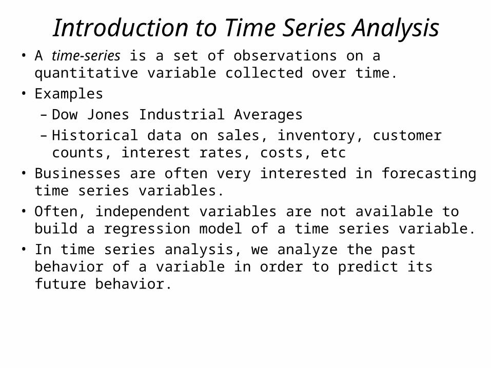
Introduction to Time Series Analysis• A time-series is a set of observations on a quantitative
variable collected over time.• Examples
– Dow Jones Industrial Averages– Historical data on sales, inventory, customer counts,
interest rates, costs, etc• Businesses are often very interested in forecasting time
series variables.• Often, independent variables are not available to build a
regression model of a time series variable.• In time series analysis, we analyze the past behavior of a
variable in order to predict its future behavior.

Methods used in Forecasting
• Regression Analysis
• Time Series Analysis (TSA)– A statistical technique that uses time-
series data for explaining the past or forecasting future events.
– The prediction is a function of time (days, months, years, etc.)
– No causal variable; examine past behavior of a variable and and attempt to predict future behavior
Components of TSA
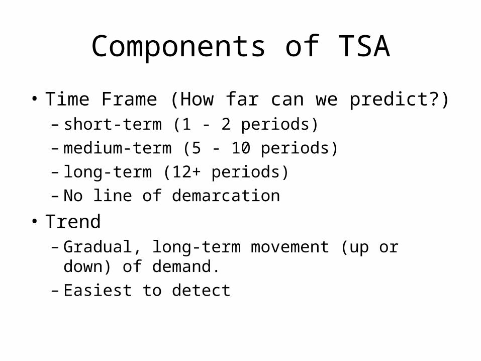
• Time Frame (How far can we predict?)– short-term (1 - 2 periods)– medium-term (5 - 10 periods)– long-term (12+ periods)– No line of demarcation
• Trend– Gradual, long-term movement (up or down) of
demand.– Easiest to detect

Components of TSA (Cont.)
• Cycle– An up-and-down repetitive movement in demand.– repeats itself over a long period of time
• Seasonal Variation– An up-and-down repetitive movement within a trend
occurring periodically.– Often weather related but could be daily or weekly
occurrence
• Random Variations– Erratic movements that are not predictable because
they do not follow a pattern

Time Series PlotActual Sales
$0
$500
$1,000
$1,500
$2,000
$2,500
$3,000
1 2 3 4 5 6 7 8 9 10 11 12 13 14 15 16 17 18 19 20 21
Time Period
Sal
es (
in $
1,00
0s)

Components of TSA (Cont.)
• Difficult to forecast demand because...– There are no causal variables
– The components (trend, seasonality, cycles, and random variation) cannot always be easily or accurately identified

Some Time Series Terms• Stationary Data - a time series variable exhibiting
no significant upward or downward trend over time.
• Nonstationary Data - a time series variable exhibiting a significant upward or downward trend over time.
• Seasonal Data - a time series variable exhibiting a repeating patterns at regular intervals over time.
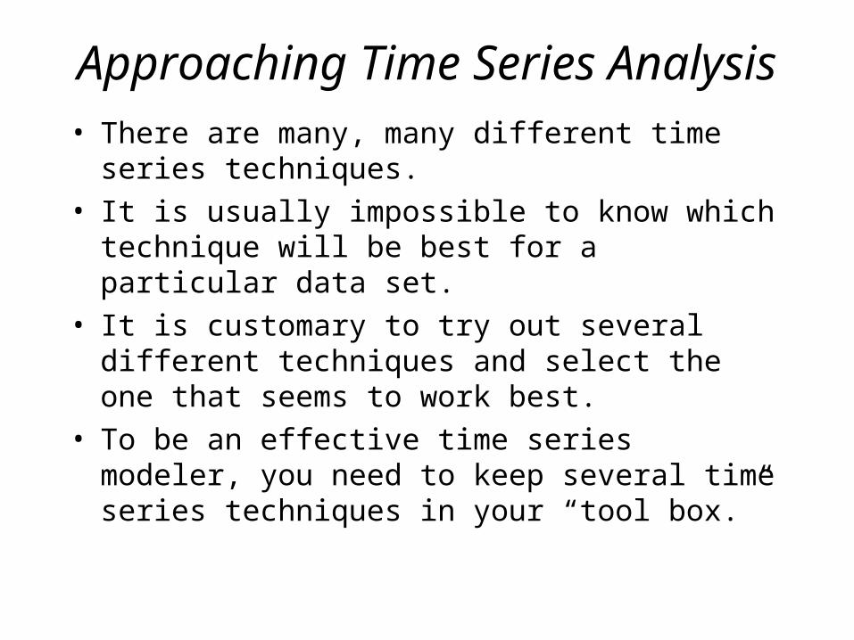
Approaching Time Series Analysis• There are many, many different time series
techniques.
• It is usually impossible to know which technique will be best for a particular data set.
• It is customary to try out several different techniques and select the one that seems to work best.
• To be an effective time series modeler, you need to keep several time series techniques in your “tool box.”

Measuring Accuracy• We need a way to compare different time series techniques for a given data set.• Four common techniques are the:
– mean absolute deviation,
– mean absolute percent error,
– the mean square error,
– root mean square error.
MAD = Y Yi i
i
n
n
1
MSE =
Y Yi i
i
n
n
2
1
MSERMSE
n
i i
ii
n 1 Y
YY100 = MAPE
• We will focus on MSE.

Extrapolation Models• Extrapolation models try to account for the past behavior
of a time series variable in an effort to predict the future behavior of the variable.
, , ,Y Y Y Yt t t tf 1 1 2
We’ll first talk about several extrapolation techniques that are appropriate for stationary data.

An Example• Electra-City is a retail store that sells audio and video
equipment for the home and car. • Each month the manager of the store must order
merchandise from a distant warehouse. • Currently, the manager is trying to estimate how many
VCRs the store is likely to sell in the next month. • He has collected 24 months of data.•

Moving Averages
YY Y Yt t-1 t- +1
tk
k
1
No general method exists for determining k.
We must try out several k values to see what works best.
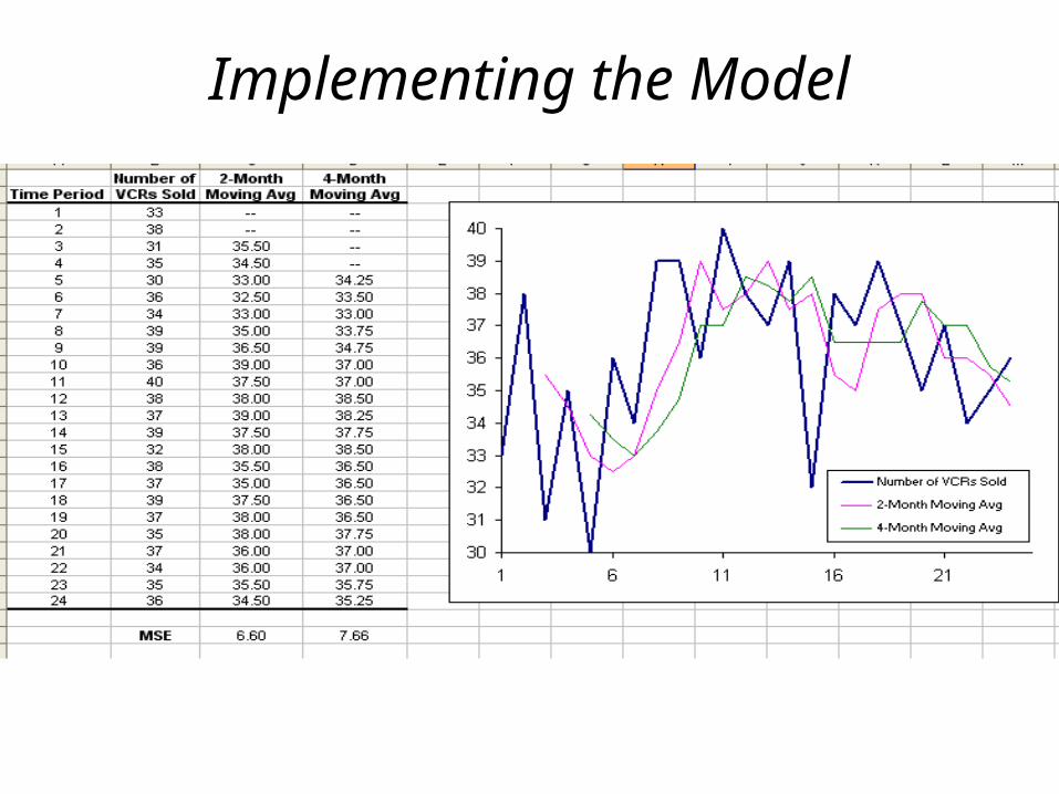
Implementing the Model

A Comment on Comparing MSE Values
• Care should be taken when comparing MSE values of two different forecasting techniques.
• The lowest MSE may result from a technique that fits older values very well but fits recent values poorly.
• It is sometimes wise to compute the MSE using only the most recent values.

Forecasting With The Moving Average Model
.YY Y
2
36 + 35
22524 23 355
Forecasts for time periods 25 and 26 at time period 24:
.YY Y
2
35.5 + 36
22625 24 3575

Weighted Moving Average• The moving average technique assigns equal weight
to all previous observations
Y1
Y1
Y1
Yt t-1 t- -1t kk k k 1
The weighted moving average technique allows for different weights to be assigned to previous observations.
Y Y Y Yt t-1 t- -1t k kw w w 1 1 2
where 0 and w wi i1 1
We must determine values for k and the wi

Implementing the Model

Using optimal values for the weights that minimizes the MSE

Forecasting With The Weighted Moving Average Model
. . .Y Y Y25 1 24 2 23 0 291 36 0 709 35 35 3 w w
Forecasts for time periods 25 and 26 at time period 24:
80.3536709.03.35291.0YYY 24225126 ww

Exponential Smoothing
( )Y Y Y Yt t t t 1 where 0 1
It can be shown that the above equation is equivalent to:
( ) ( ) ( )Y Y Y Y Yt t t tn
t n 1 12
21 1 1
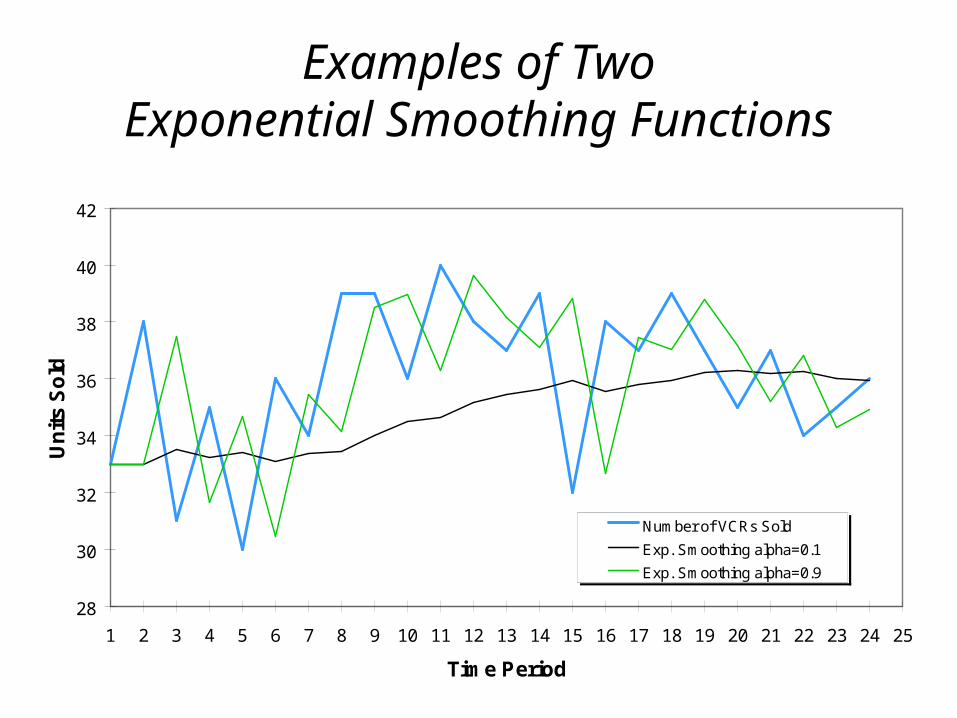
Examples of TwoExponential Smoothing Functions
28
30
32
34
36
38
40
42
1 2 3 4 5 6 7 8 9 10 11 12 13 14 15 16 17 18 19 20 21 22 23 24 25
Time Period
Un
its
So
ld
Number of VCRs Sold
Exp. Smoothing alpha=0.1
Exp. Smoothing alpha=0.9

Implementing the Model

Forecasting With The Exponential Smoothing Model
( ) . . ( . ) .Y Y Y Y25 24 24 24 35 74 0 268 36 35 74 3581
Forecasts for time periods 25 and 26 at time period 24:
( ) ( ) .Y Y Y Y Y Y Y Y26 25 25 25 25 25 25 25 3581
. ,Y for = 25, 26, 27, t t3581
Note that,

Seasonality
• Seasonality is a regular, repeating pattern in time series data.
• May be additive or multiplicative in nature...

Multiplicative Seasonal Effects
1 2 3 4 5 6 7 8 9 10 11 12 13 14 15 16 17 18 19 20 21 22 23 24 25
Tim e Pe riod
Additive Seasonal Effects
1 2 3 4 5 6 7 8 9 10 11 12 13 14 15 16 17 18 19 20 21 22 23 24 25
Tim e Pe riod
Stationary Seasonal Effects

Stationary Data With Additive Seasonal Effects
pnttnt SEYwhere
1)E-(1)S-Y(E tt-ptt
ptttt )S-(1)E-Y(S
10
10
p represents the number of seasonal periods
• Et is the expected level at time period t.
• St is the seasonal factor for time period t.

Implementing the Model

Forecasting With The AdditiveSeasonal Effects Model
Forecasts for time periods 25 - 28 at time period 24:
4242424 SEY nn
00.36345.855.354SEY 212425 73.33682.1755.354SEY 222426
13.40158.4655.354SEY 232427 82.32273.3155.354SEY 242428

Stationary Data With Multiplicative Seasonal Effects
pnttnt SEYwhere
1)E-(1)/SY(E tt-ptt
ptttt )S-(1)/EY(S
10
10
p represents the number of seasonal periods
• Et is the expected level at time period t.
• St is the seasonal factor for time period t.

Implementing the Model

Forecasting With The MultiplicativeSeasonal Effects Model
Forecasts for time periods 25 - 28 at time period 24:
4242424 SEY nn
26.359015.195.353SEY 212425 83.334946.095.353SEY 222426
03.401133.195.353SEY 232427 80.322912.095.353SEY 242428

Trend Models• Trend is the long-term sweep or general
direction of movement in a time series.• We’ll now consider some nonstationary time
series techniques that are appropriate for data exhibiting upward or downward trends.

An Example• WaterCraft Inc. is a manufacturer of personal water crafts (also known as jet
skis). • The company has enjoyed a fairly steady growth in sales of its products.• The officers of the company are preparing sales and manufacturing plans
for the coming year. • Forecasts are needed of the level of sales that the company expects to
achieve each quarter.

Double Exponential Smoothing(Holt’s Method)
• Et is the expected base level at time period t.
• Tt is the expected trend at time period t.
• n is the period-ahead forecast made in period t.
ttnt nTEY
where
Et = Yt + (1-)(Et-1+ Tt-1)
Tt = (Et Et-1) + (1-) Tt-10 1 1 and 0

Implementing the Model

Using optimal values for α and ß that minimizes the MSE

Forecasting With Holt’s Model
Forecasts for time periods 21 through 24 at time period 20:
. . .Y E T21 20 201 2336 8 1 152 1 2488 9 . . .Y E T22 20 202 2336 8 2 152 1 26410 . . .Y E T23 20 203 2336 8 3 152 1 27931 . . .Y E T24 20 204 2336 8 4 152 1 2945 2
202020 TEY nn

Holt-Winter’s Method For Additive Seasonal Effects
pntttnt n STEYwhere
)T)(E-(1SYE 11 ttpttt 11 )T-(1EET tttt ptttt )S-(1EYS
10
10
10

Implementing the Model

The Linear Trend Model
Y Xt b bt
0 1 1
where X1tt
For example:X X X 1 1 11 2 3
1 2 3 , , ,

Implementing the Model

Forecasting With The Linear Trend Model
Forecasts for time periods 21 through 24 at time period 20:
. . .Y X21 0 1 1213751 92 6255 21 2320 3 b b
. . .Y X22 0 1 1223751 92 6255 22 2412 9 b b
. . .Y X23 0 1 1233751 92 6255 23 25056 b b
. . .Y X24 0 1 1243751 92 6255 24 2598 2 b b

The TREND() Function
TREND(Y-range, X-range, X-value for prediction)where:
Y-range is the spreadsheet range containing the dependent Y variable,
X-range is the spreadsheet range containing the independent X variable(s),
X-value for prediction is a cell (or cells) containing the values for the independent X variable(s) for which we want an estimated value of Y. Note: The TREND( ) function is dynamically updated whenever any inputs to the function change. However, it does not provide the statistical information provided by the regression tool. It is best two use these two different approaches to doing regression in conjunction with one another.

The Quadratic Trend Model
Y X Xt b b bt t
0 1 1 2 2
where X and X1 22
t tt t
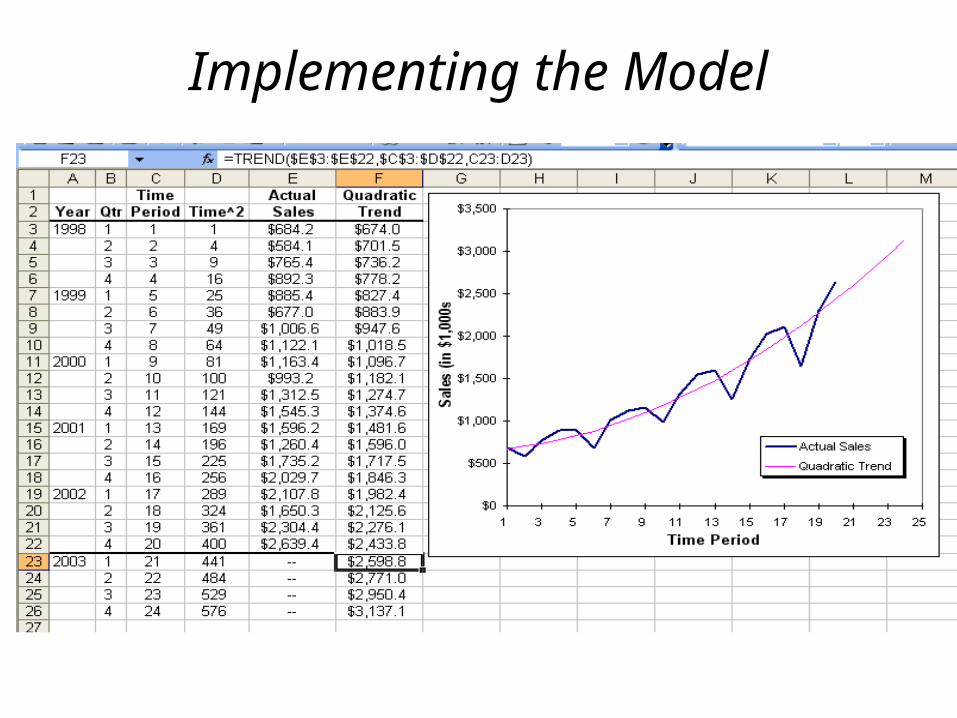
Implementing the Model

Forecasting With The Quadratic Trend Model
Forecasts for time periods 21 through 24 at time period 20:
8.259821617.321671.1667.653XXY 22211021 2121
bbb
0.277122617.322671.1667.653XXY 22211022 2222
bbb
4.295023617.323671.1667.653XXY 22211023 2323
bbb
1.313724617.324671.1667.653XXY 22211024 2424
bbb

Computing Multiplicative Seasonal Indices
• We can compute multiplicative seasonal adjustment indices for period p as follows:
S
Y
Y, for all occuring in season p
i
ii
pni p
The final forecast for period i is then Y adjusted = Y S , for any occuring in season i i p i p

Implementing the Model

The Plot

Forecasting With Seasonal Adjustments Applied To Our Quadratic Trend Model
Forecasts for time periods 21 through 24 at time period 20:
8.2747%7.1059.2598)XX(Y 12211021 2121 Sbbb
6.2219%1.801.2771)XX(Y 22211022 2222 Sbbb
4.3041%1.1035.2950)XX(Y 32211023 2323 Sbbb
1.3486%1.1112.3137)XX(Y 42211024 2424 Sbbb

Summary of the Calculation and Use of Seasonal Indices
1. Create a trend model and calculate the estimated value for each observation in the sample.
2. For each observation, calculate the ratio of the actual value to the predicted trend value:
(For additive effects, compute the difference:
3. For each season, compute the average of the ratios calculated in step 2. These are the seasonal indices.
4. Multiply any forecast produced by the trend model by the appropriate seasonal index calculated in step 3. (For additive seasonal effects, add the appropriate factor to the forecast.)
tY
.Y/Y tt
).YY tt

Refining the Seasonal Indices
• Note that Solver can be used to simultaneously determine the optimal values of the seasonal indices and the parameters of the trend model being used.
• There is no guarantee that this will produce a better forecast, but it should produce a model that fits the data better in terms of the MSE.

Seasonal Regression Models• Indicator variables may also be used in regression
models to represent seasonal effects.• If there are p seasons, we need p-1 indicator variables. Our example problem involves quarterly data, so p=4
and we define the following 3 indicator variables:
X if Y is an observation from quarter 2
otherwise4
1
0t
t
,
,
X if Y is an observation from quarter 1
otherwise3
1
0t
t
,
,
X if Y is an observation from quarter 3
otherwise5
1
0t
t
,
,

Implementing the Model
• The regression function is:Y X X X X Xt b b b b b b
t t t t t 0 1 1 2 2 3 3 4 4 5 5
where X and X1 22
t tt t

The Data

The Regression Results

The Plot

Forecasting With The Seasonal Regression Model
Forecasts for time periods 21 through 24 at time period 20:
5.2638)0(453.123)0(736.424)1(805.86)21(485.3)21(319.17471.824Y 221
7.2467)0(453.123)1(736.424)0(805.86)22(485.3)22(319.17471.824Y 222
2.2943)1(453.123)0(736.424)0(805.86)23(485.3)23(319.17471.824Y 223
8.3247)0(453.123)0(736.424)0(805.86)24(485.3)24(319.17471.824Y 224

Combining Forecasts
• It is also possible to combine forecasts to create a composite forecast.• Suppose we used three different forecasting methods on a given data
set.
Denote the predicted value of time period t using each method as follows:
F F Ft t t1 2 3, , and
We could create a composite forecast as follows:
Y F F Ft b b b bt t t
0 1 1 2 2 3 3