TIME-SEQUENTIAL EXTRACTION OF MOTION LAYERS

Matthieu Fradet, Patrick Perez* and Philippe Robert

Thomson Corporate Research, Rennes, France, *INRIA, Rennes - Bretagne Atlantique, France

ABSTRACT

A new time-sequential approach for motion layer extraction is pre-sented. We assume that the scene can be described by a set of lay-ers associated to affine motion models. In one or more key frames,the segmentation is obtained using a semi-automatic method. At asubsequent instant, the first step of the proposed algorithm is theprediction of the segmentation from one image to the next one, us-ing motion models estimated for each layer. The second step is therefinement of the predicted motion boundaries by graph cut. Onlythe appearing areas and a strip around the predicted boundaries arequestioned. A new rigidity constraint improves the temporal consis-tency of foreground rigid objects. Experimental results show that oursequential approach is at least as effective as more complex simulta-neous approaches while being less computationally demanding.

Index Terms— Motion Analysis, Video Segmentation, MotionLayers, Motion Boundaries, Graph Cut.

1. INTRODUCTION

Despite its long history, the problem of segmenting video in regionsof similar motion is still a very active research topic in computer vi-sion. Motion layer extraction has many applications, such as videocompression, mosaic generation, video object removal, etc. More-over the extracted layers can be used for advanced video editing tasksincluding matting and compositing.

The usual assumption is that a scene can be approximated by aset of layers whose motions in the image plane are well described bya parametric model. Motion segmentation consists in estimating themotion parameters of each layer and in extracting the layer supports.

There are many different approaches. Only examples from dif-ferent classes are mentioned below.

In [1] a dense motion field previously estimated is segmented.Parametric models are iteratively a) estimated on rough regions,b) used to refine the regions and c) finally updated according to thenew supports . Once convergence is obtained, segmentation map ispredicted for the next image, new motion models are estimated, etc.

Some authors [2, 3] propose to combine dense motion estima-tion and parametric segmentation, while some others extract layerseither jointly [4], or one after another [5] using a direct parametricsegmentation with no optical flow computation.

More recently, video segmentation was formulated into thegraph cut framework. Sequential approaches such as [6] provide asegmentation map for the current image taking into account the pre-vious labeling only. But the whole segmentation is questioned againin the subsequent image, at the expense of temporal consistency.

Some researchers moved naturally to simultaneous batch ap-proaches [7, 8] to increase temporal consistency. To do so, they use3D graphs at the pixel level that allow the simultaneous segmentationof N images. Such methods remove certain artifacts that successive2D graph optimizations can create. ([8] presents a method to extract

Fig. 1. Simplified Flow Chart of our Algorithm.

the hidden parts of motion layers too, but in this paper we consideronly the visible parts.)

The main limitation of simultaneous approaches is their compu-tational complexity. The number N of processed images can cer-tainly not cover a whole sequence due to complexity issues. Also,assuming all pixel labels unknown within the temporal window ofinterest does not allow any restriction of the area on which the graphis built.

In contrast, we introduce a time-sequential approach which, withmodest user input in one or few frames, provides results at least asgood as those obtained by latter batch approaches at a lower compu-tational cost.

In our work, we assume that the layers keep the same depth orderduring the whole sequence. On the first image, as well as on fewsubsequent images if necessary, the segmentation is obtained usingan interactive graph cut-based method that exploits both motion andcolor information.

At current time t, the segmentation of image It is first predictedby projection of the previous segmentation. A dense forward mo-tion field between It and It+1 and a backward motion field betweenIt and It−1 are estimated. Based on them, forward and backwardaffine motion models are estimated for each layer according to thepredicted segmentation. Predicted motion boundaries are finally re-fined using graph cut to minimize an energy composed of motion,color, spatial smoothness, temporal terms and a new rigidity con-straint term. This is continued for all the images of the sequence.

A simplified flow chart of our sequential system after initializa-tion is shown in Figure 1.

The paper is organized as follows. Section 2 addresses user in-teraction. Section 3 presents the graph restriction and our motionboundaries propagation and refinement algorithm. Experimental re-sults are shown in Section 4.

2. INTERACTIVE SEGMENTATION OF ONE IMAGE

This step is systematically required for the first frame, but can alsobe used later in the sequence for re-initialization if needed.

For the considered image It, the user provides some large andloose seeds to mark the n different layers. These seeds are generally

Fig. 2. Example of polygonal seeds given by the user. Left to right:original image, seeds, obtained segmentation in 5 layers. Depth dis-play convention: the darker is the seed, the more distant is the layer.

polygonal regions, ordered by depth. An example of such seeds isgiven in Figure 2.

The seeds are used as layer supports to compute Gaussian Mix-ture Models (GMMs) in the RGB space. They are also used jointlywith a forward dense motion field to estimate one affine motionmodel per layer.

Given the labeling f = (fp)p∈P with fp ∈ [0, n− 1] and Pthe pixel set to be segmented, we consider the following objectivefunction, which is the sum of two standard terms (color data termand spatial smoothness) described in [9], and of the motion-basedterm described in [7]:

E(f) =∑p∈P

Cp(fp)︸ ︷︷ ︸Ecolor(f)

+λ1

∑(p,q)∈C

Vp,q(fp, fq)︸ ︷︷ ︸Esmooth(f)

+λ2

∑p∈P

Dp(fp)︸ ︷︷ ︸Emotion(f)

(1)

Dp(fp) = arctan(‖It(p)− It+1(p’)‖2 − τ1) +π

2(2)

where C is the set of neighbor pairs with respect to 8-connectivity,and λ1 and λ2 are positive parameters which weight the influence ofeach term.

Cp(fp) is a standard color data penalty term at pixel p, set asthe negative log-likelihood of color distribution of the layer fp. Thisdistribution consists of the GMM computed on the seeds of the layerfp.

Vp,q(fp, fq) is a standard contrast-sensitive regularization term.Dp(fp) is a data penalty term at pixel p for the motion model

corresponding to layer fp (p’ is the correspondent in It+1 of p inIt according to this parametric motion model). This smooth penaltyand its threshold parameter τ1 allow a soft distinction between lowresiduals (well classified pixels) and high residuals (wrongly classi-fied pixels or occluded pixels). In our experiments we chose τ1 =50. Adding this motion term solves more easily ambiguities due tocolors, with no need for the user to introduce additional seeds. If twodifferent objects have similar colors but different motions, an inter-active method based on colors only would force the user to provideadditional seeds in such regions.

3. MOTION BOUNDARIES REFINEMENT

3.1. Graph Restriction

In our sequential approach, we propose to predict the labeling, andhence motion boundaries, from the previous instant and to consider,around these predicted boundaries, an uncertainty strip in which la-beling can be modified. Notice that appearing areas have no pre-dicted labels. That is why they are also considered as uncertain. Inthe other areas, we assume that the predicted labels are correct andassociated pixels are ignored by the graph. Such an assumption re-duces significantly the size of the graph and constrains the segmen-tation both spatially and temporally.

Fig. 3. Graph Restriction. Case of a moving foreground object anda stationary background. (Left, previous segmentation already ob-tained.)

Figure 3 illustrates this graph restriction in a binary case. Thewidth w of the uncertainty strip is defined by the user. In our ex-periments we chose w = 12. It includes 5 pixels on each side ofthe boundaries, and 1 more pixel on each side to have boundary con-ditions. Pixels belonging to these 1-pixel strips are considered asseeds and provide hard constraints which are satisfied by setting tospecific values the weights of the links that connect these seeds withthe terminals (see [9]).

This way to build the graph is particularly well adapted to ourmotion boundaries refinement.

3.2. Objective Function

Moreover, to increase the effect of temporal consistency, not only thecurrently processed image and the previous one but also the next im-age are taken into account, to form a triplet. Forward and backwardmotion fields are consequently estimated. We compare these twofields to improve accuracy of the estimated vectors in the occlusionareas. A reliability index, based on the Displaced Frame Difference(DFD) is computed for every motion vector of both fields:

rα(p)=max(0, 1−‖It(p)− It+α(p − dpα)‖τ2

), α∈{−1,+1} (3)

where dpα is the motion vector, either forward or backward, esti-mated at pixel p and τ2 is an empirical normalization threshold.

Then for a pixel whose forward vector has a lower reliabilitythan its backward vector, we correct the forward field by replacingthe forward vector with the opposite of the backward one. The samecorrection is done for the backward field. This correction improvesthe estimated motion fields before the motion model approximationstep. At the end of this motion estimation step, two corrected mo-tion fields (forward and backward) and their associated pixel-wisereliability maps are available.

The motion model parameters of each layer are recovered by astandard linear regression technique but we use the reliability mea-sure to weight the influence of each vector on the model.

The energy to be minimized at current instant extends (1) asfollows:

• The set of pixelsP is only a fraction of the original pixel grid,as explained in 3.1.

• We keep the same expressions for color data and spatialsmoothness terms.

• We adapt the motion data term to our triplet-based sequentialsetup. Thus, (2) becomes

Dp(fp)= minα∈{−1,+1}

(arctan(‖It(p)− It+α(p’α)‖2−τ1)+π

2) (4)

where p’α is the correspondent in It+α of p in It accordingto the affine motion model of the layer fp.

• Like in [6, 7, 8], we introduce a fourth term to enforce tem-poral constraints. It maintains the temporal consistency ofthe segmentation between current frame It and frame It−1

already segmented. Thanks to the estimated motion models,we define the temporal term as follows:

Etemp(f) =∑p∈P

ψ(p) (5)

ψ(p) =

{1 if fp 6= fp’ and f ′p 6= ∅0 otherwise

(6)

where p’ is the correspondent of p in It−1 according to thebackward model of the layer fp, f ′p is the predicted label ofpixel p at instant t, and ∅ is the blank label for the appearingareas without any predicted label.

• We add, when appropriate, a new rigidity constraint to in-crease temporal consistency of foreground layers that remainnon-occluded and to avoid, this way, the insertion of the cor-responding labels in the appearing areas:

Erigid(f) =∑p∈P

φ(p) (7)

φ(p) =

{1 if fp ∈ Srigid and f ′p = ∅0 otherwise

(8)

where Srigid is the set of labels corresponding to the layerson which the rigidity constraint is applied.

The global energy to be minimized at every instant is:

E(f) = Ecolor(f) + λ1Esmooth(f) + λ2Emotion(f)

+ λ3Etemp(f) + λ4Erigid(f) (9)

where λ1, λ2, λ3 and λ4 are positive parameters which weight theinfluence of each term. They are set by the user and depend on thereliability of the motion estimation and on the characteristics of thesequence. Energies (1) and (9) are minimized using graph cuts [10,11]. As we want to handle an arbitrary number of layers, we use theα-expansion algorithm [12] to solve the multi-labels problem.

4. EXPERIMENTAL RESULTS

The proposed algorithm was tested on the same three sequences thatare shown in [6, 7, 8]. Our algorithm provides dense segmentationmaps without any additional label for noise, occluded pixels or inde-termination (contrary to [7, 8]).

Figure 4 shows our results on the Calendar sequence. Only oneadditional user interaction on frame 40 was required. The obtainedsegmentations are correct even at the end of the sequence, which isusually not processed, where the ball and the train regions are not incontact anymore. Thanks to our rigidity constraint the ball supportnever stretches over similar color regions of the background.

Figure 5 shows the satisfactory results obtained for the Flowerssequence even when the user only provides a segmentation map forthe first image. Branches structures are really thin and their preciseextraction would require a matting method.

Concerning the Carmap sequence, the main difficulty is thelarge occlusion of the car whose front is hidden by the foregroundmap at the beginning, and whose wheels and shadow are black likethe map edges. Moreover the motions of the map (notably the stem)and of the background are almost similar.

Figure 6 shows the results obtained when the user providedrough segmentation for the images 1 and 11, with and without rigid-ity constraint on the map layer. The simultaneous approaches seemto encounter the same difficulty to classify as “car” the front of thecar as soon as it appears to the right of the map. The contributionof the rigidity constraint is noticeable: it avoids classification mis-takes in uniform dark areas (wheels, shadow of the car and edgesof the map) where neither the color term nor the motion term aresufficiently discriminative. Notice that even the stem of the map iswell segmented.

sequence image size mean graph size n CPU/frameCalendar 352 x 240 11647 pix. 4 ∼ 6 s.Flowers 352 x 240 22886 pix. 4 ∼ 6 s.Carmap 320 x 240 9192 pix. 3 ∼ 3 s.

Table 1. Mean CPU times including all processings. (n is the num-ber of layers).

All the experiments were performed on a P-4 3.6GHz machine.Including all processings (motion estimation, GMMs computation,graph construction, labeling . . . ), the time required for the segmen-tation of one image mainly depends on the number of layers (seeTable 1). In [7], the segmentation of one image is less than 30 sec-onds in average on a P-4 2.0GHz machine.

5. CONCLUSION

We presented a new sequential algorithm for motion layer extrac-tion. We propose to predict motion boundaries from one image tothe next one and to refine them by graph cut. Only the appearingareas and a strip around the predicted boundaries are questioned.Results show that our sequential method is less expensive than com-plex simultaneous methods while providing results of at least similarquality. It includes an original rigidity constraint whose usefulnesswas demonstrated. Moreover the user can interrupt the system assoon as a segmentation map is not satisfactory, without having towait that the whole sequence is processed. However it turns out thatsuch interactions are rarely required.

The interactive initialization step could be avoided using an au-tomatic process to estimate the number of layers and their initial pa-rameters (e.g. split and merge process repeated until stability). Butnote that if the initial segmentation is not accurate enough or if theestimated number of layers is not appropriate, our algorithm will notinsure a fast convergence to expected segmentations.

In future work, we will integrate in our algorithm a step of gen-eration of layer mosaic to store the disappearing areas. Such pro-gressively built mosaics could help the segmentation of subsequentimages, notably in cases where disappeared areas reappear later inthe sequence after long occlusions.

6. REFERENCES

[1] J. Wang and E. Adelson, “Representing moving images withlayers,” IEEE Trans. on Image Processing, vol. 3, no. 5, pp.625–638, September 1994.

[2] M. J. Black and P. Anandan, “The robust estimation of mul-tiple motions: Parametric and piecewise-smooth flow fields,”Computer Vision and Image Understanding, vol. 63, no. 1, pp.75–104, 1996.

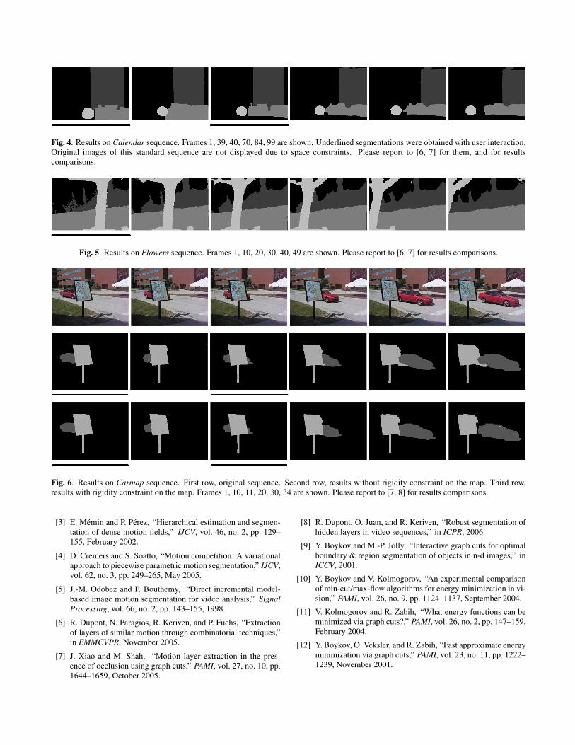
Fig. 4. Results on Calendar sequence. Frames 1, 39, 40, 70, 84, 99 are shown. Underlined segmentations were obtained with user interaction.Original images of this standard sequence are not displayed due to space constraints. Please report to [6, 7] for them, and for resultscomparisons.

Fig. 5. Results on Flowers sequence. Frames 1, 10, 20, 30, 40, 49 are shown. Please report to [6, 7] for results comparisons.

Fig. 6. Results on Carmap sequence. First row, original sequence. Second row, results without rigidity constraint on the map. Third row,results with rigidity constraint on the map. Frames 1, 10, 11, 20, 30, 34 are shown. Please report to [7, 8] for results comparisons.

[3] E. Memin and P. Perez, “Hierarchical estimation and segmen-tation of dense motion fields,” IJCV, vol. 46, no. 2, pp. 129–155, February 2002.

[4] D. Cremers and S. Soatto, “Motion competition: A variationalapproach to piecewise parametric motion segmentation,” IJCV,vol. 62, no. 3, pp. 249–265, May 2005.

[5] J.-M. Odobez and P. Bouthemy, “Direct incremental model-based image motion segmentation for video analysis,” SignalProcessing, vol. 66, no. 2, pp. 143–155, 1998.

[6] R. Dupont, N. Paragios, R. Keriven, and P. Fuchs, “Extractionof layers of similar motion through combinatorial techniques,”in EMMCVPR, November 2005.

[7] J. Xiao and M. Shah, “Motion layer extraction in the pres-ence of occlusion using graph cuts,” PAMI, vol. 27, no. 10, pp.1644–1659, October 2005.

[8] R. Dupont, O. Juan, and R. Keriven, “Robust segmentation ofhidden layers in video sequences,” in ICPR, 2006.

[9] Y. Boykov and M.-P. Jolly, “Interactive graph cuts for optimalboundary & region segmentation of objects in n-d images,” inICCV, 2001.

[10] Y. Boykov and V. Kolmogorov, “An experimental comparisonof min-cut/max-flow algorithms for energy minimization in vi-sion,” PAMI, vol. 26, no. 9, pp. 1124–1137, September 2004.

[11] V. Kolmogorov and R. Zabih, “What energy functions can beminimized via graph cuts?,” PAMI, vol. 26, no. 2, pp. 147–159,February 2004.

[12] Y. Boykov, O. Veksler, and R. Zabih, “Fast approximate energyminimization via graph cuts,” PAMI, vol. 23, no. 11, pp. 1222–1239, November 2001.