Time-evolving Graph Processing on Commodity Clusters: Spark Summit East talk by Anand Iyer

TegraTime-evolving Graph Processing on Commodity Clusters

Anand Iyer Joseph GonzalezQifan Pu Ion Stoica

Spark Summit East8 February 2017

About Me1

• PhD Candidate at AMP/RISE Lab at UC Berkeley• Thesis on time-evolving graph processing• Previous work:• Collaborative energy diagnosis for smartphones

(carat.cs.berkeley.edu)• Approximate query processing (BlinkDB)• Cellular Network Analytics• Fundamental trade-offs in applying ML to real-time datasets

Graphs are everywhere…

Social Networks

2


Gnutella network subgraph

3

Graphs are everywhere…4


Metabolicnetworkofasinglecellorganism Tuberculosis

5

Plenty of interest in processing them

• Graph DBMS 25% of all enterprises by end of 20171

• Many open-source and research prototypes on distributed graph processing frameworks: Giraph, Pregel, GraphLab, GraphX, …

1Forrester Research

6

Real-world Graphs are Dynamic

EarthquakeOccurrenceDensity

7

Real-world Graphs are Dynamic8

Real-world Graphs are Dynamic9

Processing Time-evolving Graphs

Many interesting business and research insights possible by processing such dynamic graphs…

10

… little or no work in supporting such workloads in existing graph-processing frameworks

Challenge #1: Storage11

Time

A

B C

G1

A

B C

D

G2

Redundant storage of graph entities over time

A

B C

DE

G3

Challenge #2: Computation12

A

B C

R1

A

B C

DE

R3

Wasted computation across snapshots

Time

A

B C

G1

A

B C

D

G2

A

B C

DE

G3

A

B C

D

R2

Challenge #3: Communication13

A

B C

A

B C

D A

B C

D

E

Time

A

B C

G1

A

B C

D

G2

A

B C

DE

G3

Duplicate messages sent over the network

How do we process time-evolving, dynamically changing graphs

efficiently?

14

Share StorageCommunicationComputation

Tegra


efficiently?

15


Tegra

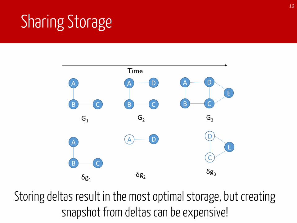
Sharing Storage16

Time

A

B C

G1

A

B C

δg1

A D

δg2

A

B C

D

G2

A

B C

DE

G3

C

DE

δg3

Storing deltas result in the most optimal storage, but creating snapshot from deltas can be expensive!

A Better Storage Solution17

Snapshot 2Snapshot 1t1 t2

Use a persistent datastructure

Store snapshots in Persistent Adaptive Radix Trees (PART)

Graph Snapshot Index18

Snapshot 2Snapshot 1

Vert

ex

t1 t2

Snapshot 2Snapshot 1t1 t2

Edge

Partition

Snapshot ID Management

Shares structure between snapshots, and enables efficient operations


efficiently?

19


Tegra

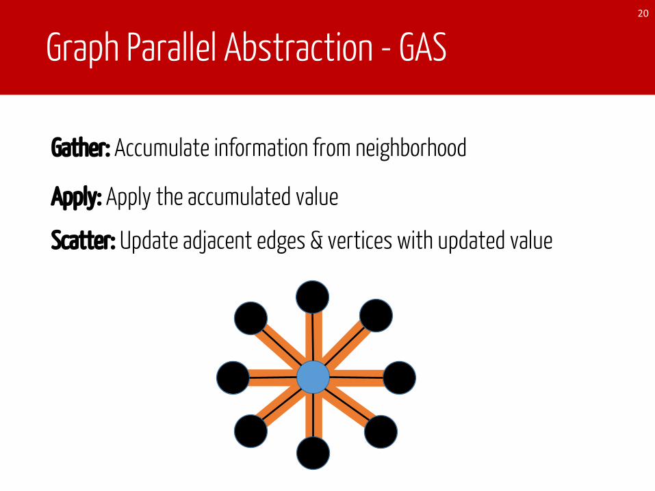
Graph Parallel Abstraction - GAS

Gather: Accumulate information from neighborhood

20

Apply: Apply the accumulated value

Scatter: Update adjacent edges & vertices with updated value

Processing Multiple Snapshots21

for (snapshot in snapshots) {for (stage in graph-parallel-computation) {…}

}

A

B C

A

B C

D A

B C

DE

Time

G1 G2 G3

Reducing Redundant Messages22

A

B C

A

B C

D A

B C

DE

Time

G1 G2 G3

D

BCBA

AAA

B C

DE

for (step in graph-parallel-computation) {for (snapshot in snapshots) {…}

}

Can potentially avoid large number of redundant messages


efficiently?

23


Tegra

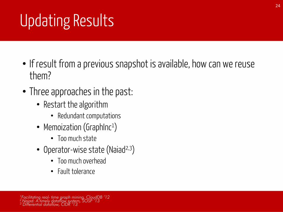
Updating Results

• If result from a previous snapshot is available, how can we reuse them?• Three approaches in the past:• Restart the algorithm

• Redundant computations

• Memoization (GraphInc1)• Too much state

• Operator-wise state (Naiad2,3)• Too much overhead• Fault tolerance

24

1Facilitating real- time graph mining, CloudDB ’122 Naiad: A timely dataflow system, SOSP ’133 Differential dataflow, CIDR ‘13

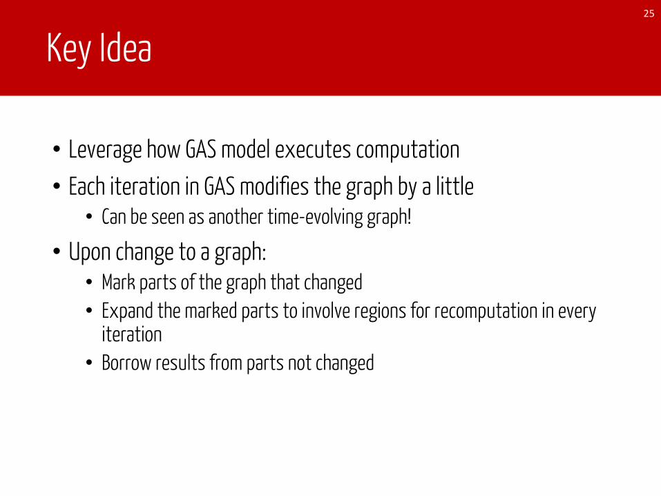
Key Idea

• Leverage how GAS model executes computation• Each iteration in GAS modifies the graph by a little• Can be seen as another time-evolving graph!

• Upon change to a graph:• Mark parts of the graph that changed• Expand the marked parts to involve regions for recomputation in every

iteration• Borrow results from parts not changed

25

Incremental Computation26

A

B C

D

Iterations

Time

A

A B

A A

A A

A

G10 G1

1 G12

G22

A

B C

A

A B

A

A A

G20 G2

1

Larger graphs and more iterations can yield significant improvements

API

val v = sqlContext.createDataFrame(List( ("a", "Alice"), ("b", "Bob"), ("c", "Charlie")

)).toDF("id", "name")

val e = sqlContext.createDataFrame(List( ("a", "b", "friend"), ("b", "c", "follow"), ("c", "b", "follow)

)).toDF("src", "dst", "relationship")

val g = GraphFrame(v, e)

27

val g1 = g.update(v1, e1)

.indexed()

.indexed()

API: Incremental Computations


28

val g1 = g.update(v1,e1)

val result1 = g1.triangleCount.run(result)

val result = g.triangleCount.run()

API: Computations on Multiple Graphs


val g1 = g.update(v1,e1)

29

val g2 = g1.update(v2,e2)

val g3 = g1.update(v3,e3)

val results = g3.triangleCount.runOnSnapshots(start, end)

API30

B C

A D

F E

A DD

B C

D

E

AA

F

B C

A D

F E

A DD

B C

D

E

AA

F

Transition

(0.977, 0.968)

(X , Y): X is 10 iteration PageRank Y is 23 iteration PageRank

After 11 iteration on graph 2,Both converge to 3-digit precision

(0.977, 0.968)(0.571, 0.556)

1.224

0.8490.502

(2.33, 2.39)

2.07

0.8490.502

(0.571, 0.556)(0.571, 0.556)

Figure 8: Example showing the benefit of PSR computation.

Streaming master program. For each iteration of Pregel,we check for the availability of a new graph. When itis available, we stop the iterations on the current graph,and resume resume it on the new graph after copyingover the computed results. The new computation willonly have vertices in the new active set continue messagepassing. The new active set is a function of the old activeset and the changes between the new graph and the oldgraph. For a large class of algorithms (e.g. incrementalPageRank [19]), the new active set includes vertices fromthe old active set, any new vertices and vertices withedge additions and deletions. Listing 2 shows a simplestreaming pagerank implementation using this API.

def StreamingPageRank(ts: TegraStream) = {def vprog(v: VertexId, msgSum: double) =

0.15+0.85*msgSumreturn ts.PSRCompute

(1, 100, EdgeDirection.Out, "10s")(vprog,triplet => triplet.src.pr/triplet.src.outDeg,(A, B) => A+B)

}

Listing 2: Page Rank Computation on Time-Evolving Graphs

Figure 8 shows a concrete example. For the first graph,it takes 23 iterations to converge to 3-digit precision. Ifwe reuse this page rank for the second updated graph onthe right, it will take another 11 iterations to converge to3-digit precision on the new graph. On the other hand,if we only finishes 10 iterations on the first graph, thentransition to the updated graph. It will take the same11 iterations to converge to 3-digit precision on the newgraph. Essentially, we saved 13 iterations.

4.2 Timelapse APITo implement the timelapse API (§3.2), we extend theGraph API in GraphX as shown in listing 3.

The API gives access to Tegra’s DGSI using the collec-tion view functions by extending them with an additional(optional) snapshot ID. By default, the snapshot ID isnot supplied, which signals Tegra to return the latestsnapshot. The timelapse computation is enabled by theextended mrTriplets7 function which now takes in an op-

7This function has been replaced by the new aggregateMessagesfunction, we simply use it for legacy reasons.

class Graph[V, E] {// Collection viewsdef vertices(sid: Int): Collection[(Id, V)]def edges(sid: Int): Collection[(Id, Id, E)]def triplets(sid: Int): Collection[Triplet]// Graph-parallel computationdef mrTriplets(f: (Triplet) => M,

sum: (M, M) => M,sids: Array[Int]): Collection[(Int, Id, M)]

// Convenience functionsdef mapV(f: (Id, V) => V,

sids: Array[Int]): Graph[V, E]def mapE(f: (Id, Id, E) => E

sids: Array[Int]): Graph[V, E]def leftJoinV(v: Collection[(Id, V)],

f: (Id, V, V) => V,sids: Array[Int]): Graph[V, E]

def leftJoinE(e: Collection[(Id, Id, E)],f: (Id, Id, E, E) => E,sids: Array[Int]): Graph[V, E]

def subgraph(vPred: (Id, V) => Boolean,ePred: (Triplet) => Boolean,sids: Array[Int]): Graph[V, E]

def reverse(sids: Array[Int]): Graph[V, E]}

Listing 3: GraphX [24] operators modified to support Tegra’stimelapse abstraction.

tional array of snapshot IDs to operate on. Internally, themrTriplets functionality is implemented using a seriesof map, join and group-by operations. By simultane-ously computing on multiple snapshots, Tegra is able toreduce the number of expensive join and group-bys. Inaddition, DGSI provides e�cient ways to perform joinwhich gives Tegra further advantages.

4.3 Dynamic ComputationsTegra uses the GAS decomposition to implement graph-parallel iterative computations. The GAS model is shownin listing 4. In this model, a vertex first accumulatesupdates from its neighbors, applies the update on itselfand then propagates the results to the neighbors. Wecan view this as a transformation of the original graph,followed by the evolution of the transformed graph. Inthis view, the transformed graph and its evolutions areorthogonal to the time-evolution of the graph, and eachsnapshot in the evolution represents one iteration of GAS.We store the transformed graph and its evolution in DGSIwith a special annotation where the prefix is taken fromthe snapshot ID which generated the transform.

Tegra can access this evolving graph in later snapshots.Intuitively, the transformed graph lets Tegra peek intoa possible future state of the graph without having toexchange messages between the vertices. This enablesthe framework to restrict the message exchanges betweenvertices to the di�erence between the previous run and thegraph changes, thus realizing a form of di�erential com-putation. It is to be noted that this is di�erent from storingand replaying messages as proposed by GraphInc [19].

8

Implementation & Evaluation

• Implemented on Spark 2.0• Extended dataframes with versioning information and iterate

operator • Extended GraphX API to allow computation on multiple

snapshots

• Preliminary evaluation on two real-world graphs• Twitter: 41,652,230 vertices, 1,468,365,182 edges• uk-2007: 105,896,555 vertices, 3,738,733,648 edges

31

0

0.5

1

1.5

2

2.5

3

3.5

4

4.5

1 2 3 4 5 6 7 8 9 10 11 12 13 14 15 16 17 18 19 20

StorageRe

duction

NumberofSnapshots

Benefits of Storage Sharing32

Datastructureoverheads

Significant improvements with more snapshots

Benefits of sharing communication33

0500100015002000250030003500400045005000

1 2 3 4 5 6 7 8 9 10 11 12 13 14 15 16 17 18 19 20

Time(s)

NumberofSnapshots

GraphX Tegra

Benefits of Incremental Computing34

0

50

100

150

200

250

0 5 10 15 20

Compu

tatio

nTime(s)

SnapshotID

Incremental FullComputation

Only 5% of the graph modified in every snapshot

50x reduction by processing only the modified part

Ongoing/Future Work

• Tight(er) integration with Catalyst• Tungsten improvements

• Code release• Incremental pattern matching• Approximate graph analytics• Geo-distributed graph analytics

35

Summary

• Processing time-evolving graph efficiently can be useful• Sharing storage, computation and communication key to efficient

time-evolving graph analysis• We proposed Tegra that implements our ideas

Please talk to us about your interesting use-cases!

[email protected]

www.cs.berkeley.edu/~api

36

Time-evolving Graph Processing on Commodity Clusters: Spark Summit East talk by Anand Iyer

Data & Analytics

Transcript of Time-evolving Graph Processing on Commodity Clusters: Spark Summit East talk by Anand Iyer