TIME DOMAIN BUFFETING ANALYSIS OF LARGE … · case study and wind field evaluation ......
118
TIME DOMAIN BUFFETING ANALYSIS OF LARGE-SPAN CABLE-STAYED BRIDGE Shuxian Hong A thesis submitted to Faculty of Engineering of University of Porto in fulfilment of the requirements for the Degree of Master in Civil Engineering, supervised by Professors Álvaro Cunha and Elsa Caetano October 2009
Transcript of TIME DOMAIN BUFFETING ANALYSIS OF LARGE … · case study and wind field evaluation ......
TIME DOMAIN BUFFETING ANALYSIS OF
LARGE-SPAN CABLE-STAYED BRIDGE
Shuxian Hong
A thesis submitted to Faculty of Engineering of University of Porto in
fulfilment of the requirements for the Degree of Master in Civil Engineering,
supervised by Professors Álvaro Cunha and Elsa Caetano
October 2009


TIME DOMAIN BUFFETING ANALYSIS OF LARGE-SPAN CABLE-STAYED BRIDGE
I
Abstract
For wind-excited vibration of long-span bridges, flutter and buffeting are the most concerning problems. Flutter is a aeroelastic instability phenomenon of bridges under a certain wind speed; while buffeting is the random vibration of bridges induced by the turbulence in the wind. Unlike flutter, the buffeting response does not generally lead to catastrophic failure. This is probably the reason why less attention has been paid to this aspect in the last several decades. However, with the record-breaking span lengths of modern suspension bridges, buffeting response has greatly increased which may cause serious fatigue damages to structural components and connections instability of vehicles traveling on the bridge deck and discomfort. Buffeting analysis is one of the most important aspects of structural reliability under turbulent wind. The classic buffeting analysis method is mainly in the frequency domain. This method cannot reflect the entire response procedure of bridge motions, and hence cannot consider the effects of instantaneous relative velocity, effective angle of attack, and structural nonlinearity.
This thesis adopts autoregressive (AR) model to simulate the wind velocity of spatial three dimensional fields, based on the built MATLAB programming. After that, time domain buffeting analysis methods are proposed to analyze the buffeting response of large-span bridges under turbulent wind and implemented in the commercial finite element package ANSYS. The unsteady self-excited forces are approximately represented by the quasi-steady theory. Aeroelastic damping and stiffness matrix for a spatial beam element are derived and incorporated into the structural finite element by using through Matrix27 element in ANSYS. After that, self-excited force is formulated as a full expression, based on Scanlan’s classic buffeting theory. At the end all these methods are applied to the Qingzhou Bridge, and the validity of presented method is verified.
KEYWORDS: Buffeting analysis, Time domain, AR model, Self-excited force, Qingzhou Bridge.


TIME DOMAIN BUFFETING ANALYSIS OF LARGE-SPAN CABLE-STAYED BRIDGE
II
Acknowledgements
My sincere gratitude goes first and foremost to Professor Alvaro Cunha , my supervisor, for his constant encouragement and guidance. He patiently motivated me to conceive and develop the main idea of the thesis. With out his guidance and inspiration, this thesis could not be successfully completed
Besides my supervisor, I would like to thank Professor Wei-Xin Ren and Xue-Lin Peng who provided me the finite element model of Qingzhou Bridge. And my gratitude is also devoted to Professor Gu Ming of State Key Laboratory for Disaster Reduction in Civil Engineering for his generously sharing of the aerodynamic coefficients of Qingzhou Bridge.
I further express my gratitude to Fernando Bastos, thanks for having read a draft of this thesis having made their precious comments and suggestions.
My deepest appreciation goes to my husband, Weihua Hu, for his great support and encouragement. And I also want to acknowledge my parents and parents-in-law. They gave me much love and warmth, enable me to overcome the frustrations which occurred in the process of writing this thesis. This thesis is dedicated to all of them.
Finally, I would like to thank everyone who directly or indirectly offered his or her help during this period.

TIME DOMAIN BUFFETING ANALYSIS OF LARGE-SPAN CABLE-STAYED BRIDGE

TIME DOMAIN BUFFETING ANALYSIS OF LARGE-SPAN CABLE-STAYED BRIDGE
GENERNAL INDEX
ABSTRACT.............................................................................................................................................I
ACKNOWLEDGEMENT ......................................................................................................................II
1. INTRODUCTION...............................................................................................................1
1.1. GENERAL.......................................................................................................................................1
1.2. CONTENTS AND OBJECTIVES OF THE STUDY ..................................................................2
2. LITERATURE REVIEW ON BRIDGE WIND ENGINEERING ..................................................................................................................................................................3
2.1. HISTORY OF THE DEVELOPMENT OF WIND ENGINEERING ..........................................3
2.2. RESEARCH METHODS OF BRIDGE WIND ENGINEERING................................................7
2.2.1 THEORETICAL ANALYSIS.............................................................................................................7
2.2.2 EXPERIMENTAL METHOD............................................................................................................7
2.2.3 NUMERICAL METHODS ................................................................................................................9
2.3. CABLE-STAYED BRIDGES AND THE PRACTICAL APPLICATION..................................9
2.4. WIND INDUCED VIBRATION OF BRIDGES .........................................................................10
2.4.1. FLUTTER .....................................................................................................................................11
2.4.2. BUFFETING .................................................................................................................................11
2.4.3 VORTEX SHEDDING....................................................................................................................11
2.4.4. GALLOPING.................................................................................................................................12
3. CHARACTERISTICS OF WIND FIELD.....................................................13
3.1. INTRODUCTION..........................................................................................................................13
3.2. MEAN WIND VELOCITY PROFILES .......................................................................................13
3.2.1 THE ‘LOGARITHMIC LAW’...........................................................................................................14
3.2.2 THE ‘POWER LAW’ ......................................................................................................................14
3.3. WIND TURBULENCE .................................................................................................................15
3.3.1. TURBULENCE INTENSITY .........................................................................................................15
3.3.2. INTEGRALS CALES OF TURBULENCE.....................................................................................16
3.3.3. SPECTRA OF LONGITUDINAL VELOCITY FLUCTUATIONS...................................................17
3.3.4. CROSS-SPECTRA OF LONGITUDINAL VELOCITY FLUCTUATIONS.....................................19

TIME DOMAIN BUFFETING ANALYSIS OF LARGE-SPAN CABLE-STAYED BRIDGE
3.3.5. SPECTRA AND CROSS-SPECTRA OF VERTICAL VELOCITY FLUCTUATIONS ................. 20
4. SIMULATION OF STOCHASTIC WIND VELOCICY FIELD ON LARGE-SPAN BRIDGES .................................................................................. 23
4.1. INTRODUCTION ......................................................................................................................... 23
4.2. SIMULATION OF STOCHASTIC WIND VELOCITY FIELD ON LARGE-SPAN BRIDGE BASED ON AUTO-REGRESSIVE MODEL ................................................................................... 24
4.2.1. CALCULATION OF COEFFICIENT MATRIX [ ]kψ ..................................................................... 25
4.2.2. CALCULATION OF THE NORMALLY DISTRIBUTED RANDOM PROCESSES ( )tN ............. 27
4.2.3. CALCULATION OF THE FLUCTUATING WIND VELOCITY ..................................................... 27
4.2.4. CALCULATION OF THE FINAL WIND VELOCITY .................................................................... 27
4.2.5. SELECTION OF THE AR MODEL RANK ................................................................................... 28
4.2.6. IMPLEMENTATION OF THE AR MODEL .................................................................................. 28
4.3. CASE STUDY AND WIND FIELD EVALUATION ................................................................ 30
4.4. CONCLUSIONS.......................................................................................................................... 35
5. TIME DOMAIN BUFFETING SIMULATION FOR WIND-BRIDGE INTERACTION ............................................................................................... 37
5.1. INTRODUCTION......................................................................................................................... 37
5.2. BUFFETING FORCE ................................................................................................................. 38
5.2.1. SLENDER BODY AND QUASI-STEADY HYPOTHESES .......................................................... 39
5.2.2 SLENDER BODY AND QUASI STEADY HYPOTHESES REMOVED: AERODYNAMIC ADMITTANCE FUNCTIONS ................................................................................................................. 40
5.3. SELF-EXCITED FORCES......................................................................................................... 41
5.3.1. QUASI-STEADY HYPOTHESIS.................................................................................................. 41
5.3.2. UNSTEADY BUFFETING............................................................................................................ 45
5.3.3. IMPLEMENTATION IN ANSYS................................................................................................... 49
6. APPLICATION OT QINGZHOU BRIDGE AND DISCUSSION ............................................................................................................................................................... 51
6.1. BRIDGE DESCRIPTION AND THE MAIN PARAMETERS ................................................ 51
6.2. FINITE ELEMENT MODELING OF QINGZHOU BRIDGE .................................................. 53
TIME DOMAIN BUFFETING ANALYSIS OF LARGE-SPAN CABLE-STAYED BRIDGE
6.2.1. SIMPLIFIED THREE-DIMENSIONAL FINITE ELEMENT MODELS OF CABLE-STAYED BRIDGES ...............................................................................................................................................53
6.2.2. FULL THREE-DIMENSIONAL FINITE ELEMENT MODELING OF THE QINGZHOU CABLE-STAYED BRIDGE ..................................................................................................................................56
6.3. TIME DOMAIN WIND VELOCITY GENERATED BY AUTO-REGRESSIVE METHOD
................................................................................................................................................................63
6.4. BUFFETING RESPONSES OF THE QINGZHOU BRIDGE ................................................69
6.4.1. CASE 1.........................................................................................................................................70
6.4.2. CASE 2.........................................................................................................................................73
7. CONCLUTIONS ..............................................................................................................................79
REFERENCES ....................................................................................................................................81
APPENDIX 1 ........................................................................................................................................87
APPENDIX 2 ........................................................................................................................................89
APPENDIX 3 ........................................................................................................................................93
APPENDIX 4 ........................................................................................................................................99

TIME DOMAIN BUFFETING ANALYSIS OF LARGE-SPAN CABLE-STAYED BRIDGE

TIME DOMAIN BUFFETING ANALYSIS OF LARGE-SPAN CABLE-STAYED BRIDGE
INDEX OF FIGURES
Fig. 2.1 - First Tay Bridge ...........................................................................................................................4
Fig. 2.2 - Collapse of Tacoma Narrows Bridge ..............................................................................................4
Fig. 2.3 - Akashi-Kaikyo Bridge, Japan ....................................................................................................6
Fig. 2.4 - Sutong Bridge, China................................................................................................................6
Fig.2.5 Full model .....................................................................................................................................6
Fig.2.6 Sectional model............................................................................................................................6
Fig. 3.1 - The atmospheric boundary layer ...........................................................................................14
Fig. 3.2 - Comparison of spectra of velocity fluctuation (z=100m, smv /3010 = ) in different codes ....19
Fig. 4.1 - Flow chart of implementing wind velocity by AR model in MATLAB ......................................30
Fig. 4.2 - Four-space points ...................................................................................................................31
Fig. 4.3 - Wind velocity curves of nodes of the example........................................................................32
Fig. 4.4 - Wind velocity power spectral density curves of nodes of the example...................................33
Fig. 4.5 - Correlation functions ...............................................................................................................34
Fig. 4.6 - Normal distribution probability function of wind velocity simulated by AR model ...................35
Fig. 5.1 - Fixed deck section immersed in a turbulent flow ....................................................................38
Fig. 5.2 - Moving deck section immersed in a laminar flow ...................................................................41
Fig. 5.3 - Space frame element of member an global coordinate system..............................................42
Fig. 5.4 - Finite element model formulated in Ansys to account for self-excited forces.........................44
Fig. 6.1 - Qingzhou cable-stayed bridge ................................................................................................52
Fig. 6.2 - Schematic representation of Qingzhou cable-stayed Bridge..................................................53
Fig. 6.3 - BEAM 4 element .....................................................................................................................55
Fig. 6.4 - BEAM 44 element ...................................................................................................................55
Fig. 6.5 - LINK 8 element .......................................................................................................................56
Fig. 6.6 - Typical mode shapes ..............................................................................................................56
Fig. 6.7 - Finite element model of Qingzhou Bridge...............................................................................60
Fig. 6.8 - Typical mode shapes ..............................................................................................................63
Fig. 6.9 - Location of points corresponding to the generation of wind speed time series......................63

TIME DOMAIN BUFFETING ANALYSIS OF LARGE-SPAN CABLE-STAYED BRIDGE
Fig. 6.10 - Simulated horizontal wind velocities at point 44, 43, 33 ...................................................... 66
Fig. 6.11 - Horizontal wind velocity power spectral density curves at point 44, 43, 33 ......................... 67
Fig. 6.12 - Correlation function .............................................................................................................. 67
Fig. 6.13 - Simulated vertical wind velocities at point 44, 43, 33........................................................... 68
Fig. 6.14 - Vertical wind velocity power spectral density curves at point 44, 43, 33 ............................. 69
Fig. 6.15 - Vertical response at mid-span of case 1 .............................................................................. 70
Fig. 6.16 - Vertical response at quarter-span of case 1 ........................................................................ 70
Fig. 6.17 - Lateral response at mid-span of case 1 ............................................................................... 70
Fig. 6.18 - Lateral response at quarter-span of case 1 ......................................................................... 71
Fig. 6.19 - Rotational response at mid-span of case 1.......................................................................... 71
Fig. 6.20 - Rotational response at quarter-span of case 1 .................................................................... 71
Fig. 6.21 - Spectrum of vertical displacement at mid-span and quarter-span....................................... 71
Fig. 6.22 - Spectrum of lateral displacement at mid-span and quarter-span ........................................ 72
Fig. 6.23 - Maximum vertical displacement along the span .................................................................. 72
Fig. 6.24 - Maximum lateral displacement along the span.................................................................... 73
Fig. 6.25 - Vertical displacement along the span under static wind forces ........................................... 73
Fig. 6.26 - Lateral displacement along the span under static wind forces ............................................ 73
Fig. 6.27 - Six flutter derivatives obtained from wind tunnel test........................................................... 75
Fig. 6.28 - Vertical response at mid-span of case 2 .............................................................................. 76
Fig. 6.29 - Vertical response at quarter-span of case 2 ........................................................................ 76
Fig. 6.30 - Lateral response at mid-span of case 2 ............................................................................... 76
Fig. 6.31 - Lateral response at quarter-span of case 2 ......................................................................... 76
Fig. 6.32 - Rotational response at mid-span of case 2.......................................................................... 76
Fig. 6.33 - Rotational response at quarter-span of case 2 .................................................................... 77
Fig. 6.34 - Variation of RMS of vertical displacement at mid span........................................................ 78

TIME DOMAIN BUFFETING ANALYSIS OF LARGE-SPAN CABLE-STAYED BRIDGE
INDEX OF TABLES Table 2.1 - List of largest cable-stayed bridges .....................................................................................10
Table 4.1 - Ascertain of AR model rank .................................................................................................34
Table 6.1 - Properties of stay cables......................................................................................................58
Table 6.2 - Material properties of structural members ...........................................................................58
Table 6.3 - Comparisons of modal analysis with (case 1) and without (case 2) initial tension..............61

TIME DOMAIN BUFFETING ANALYSIS OF LARGE-SPAN CABLE-STAYED BRIDGE

TIME DOMAIN BUFFETING ANALYSIS OF LARGE-SPAN CABLE-STAYED BRIDGE
SYMBOLS AND ABBREVIATIONS
)(tU , )(tV , )(tW - The longitudinal, vertical and transverse components of the time dependent wind
velocity vector.
( )tu - Fluctuation part of wind velocity in longitudinal dimension
U - Mean wind velocity
δ - Boundary-layer depth
0z - Roughness length
k - Von Karman’s constant
*u - Friction velocity
uI - Turbulence intensity
( )zσ - Standard derivative of ( )zu
Lux, Lu
y and Luz - Integral scales of turbulence for x, y and z direction
( )nSii - Auto spectra of the longitudinal velocity fluctuations at points i
)(nSij - Cross-spectra of longitudinal velocity fluctuations
[ ]kψ - regressive coefficient matrix
)( fCohij - coherence function of longitudinal fluctuations at points i and j
zyx CCC ,, - Decay coefficient
p – Rank of AR model
)(tFy - Drag force in the mean wind velocity direction y
)(tFz - Lift force in the direction z perpendicular to the mean wind velocity
( )tM θ - Torsional moment
F - Mean wind force
( )tFb - buffeting forces
B - deck width.
Riχ ( wuiMLDR ,;,, == ) - Complex aerodynamic admittance functions (CAAFs) which are
functions of reduced frequency
aeC - Matrix of the aerodynamic coefficients
( )θDC ( )θLC ( )θLC - Derivatives of the static coefficients with respect to the attack angle θ
( )βDC ′ , ( )βLC ′ , ( )βMC ′ - Derivatives of the static coefficients with respect to the attack angle β

TIME DOMAIN BUFFETING ANALYSIS OF LARGE-SPAN CABLE-STAYED BRIDGE
eaeK - Aeroelastic stiffness matrix for the element e
eaeC - Aeroelastic damping matrix for the element e
α and β - Proportionality coefficients for Rayleigh damping
)(tLse - Self-excited component of lift force
)(tDse - Self-excited component of drag force
)(tM se - Self-excited component of tortional moment
( )tfMα , ( )tfMh , ( )tf Lα , ( )tf Lh ( )tf Dp and ( )tf Dα are response functions due to unit impulse
displacement α (torsional), h(vertical) and p(lateral)
C - Modified damping matrix
aeC - Modified aeroelastic damping matrix
LhkC , Lhkd , kLC α , kLd α , MhkC , Mhkd , kMC α , kMd α - indicial function
*iA , *
iH (i=1,2,…,6) - Non-dimensional flutter derivatives obtained by wind tunnel tests on a cross-
section of the deck
K - Reduced velocity, UBK ω
=
ω - Angular Frequency
AR - Autoregressive
LDA - Laser Doppler Anemometry
PIV - Particle Image Velocimetry
CFD - Computational fluid dynamics
LES - Large Eddy Simulation
DES - Detached Eddy Simulation
AIC - Akaike Information Criterion
CAAF - Complex aerodynamic admittance function

TIME DOMAI BUFFETING ANALYSIS OF LARGE-SPAN CABLE-STAYED BRIDGE
1
1 INTRODUCTION
1.1 General
In 1940, the four-month-old TACOMA bridge was smashed by wind, which immediately shocked the whole world. Since then the research of wind-excited vibration of bridges have received unprecedented attention, and developed rapidly. Particularly in the recent twenty years, when very long and slender bridges have been continuously built, for which the safety under wind attack has attracted much concerns.
Turbulence induced buffeting response is one of the important concerns in the design of large span bridges. To predicate buffeting responses, Davenport [1.1] proposed a quasis-teady method and introduced aerodynamic admittance function, g(w), to consider unsteady effects. Because of the complexity of various cross-section shapes of bridge decks, Scanlan [1.2] suggested that wind tunnel
test of bridge decks be performed to determine the aerodynamic derivatives ( *iA , *
iH , *iP , i=1,…,6) ,
which are used for the expression of self-excited force. More recently, Scanlan [1.3] further interpreted the aerodynamic admittance function and gave its inherent relationship with aerodynamic derivatives. These contributions found the basis for conventional buffeting analysis. The dynamic motion equations of bridge decks are generally solved by means of response spectrum theory in frequency domain, which is estimated typically using a mode-by-mode approach that ignores the aerodynamic coupling among modes. In general, the frequency domain approach is restricted to linear structures excited by the stationary wind loads without aerodynamic nonlinearities. That is a limitation readily acceptable for design considerations under serviceability conditions but not under ultimate strength calculations.
In a time domain calculation procedure non-linear load effects or partial structural plastification may be included to provide a better and more comprehensive background for the evaluation of the safety margin at extreme load events. In order to consider the effects of instantaneous relative velocity, effective angle of attack, and structural nonlinearity, the time domain buffeting analysis is necessary.
In time domain simulation, buffeting forces are often considered through the quasi-steady formulation due to its simplicity, without considering unsteady fluid memory effects. To improve that, self-excited force is expressed in terms of convolution integrals between bridge deck motion and
TIME DOMAIN BUFFETING ANALYSIS OF LARGE-SPAN CABLE-STAYED BRIDGE
2
impulse response functions, with flutter derivatives identified from wind tunnel test. However, the flutter derivatives and admittance functions are frequency related. As an alternative, a time domain approach using indicial functions is suggested by Y. K. Lin[1.4]. In this thesis both these two approach for time domain buffeting analysis are introduced and applied to the Qingzhou Bridge, and the time domain buffeting response is obtained. 1.2 Contents and objectives of the study
The research contents are as follow:
1. Based on the built MATLAB programming, an autoregressive (AR) model is adopted to simulate the wind velocity of three dimensional fields in accordance with the time and space dependent characteristics of the 3-D fields. Then a numerical example shows the stability and reliability of this method.
2. Introduce the general idea of the buffeting and self-excited forces acting on a rigid segment of a bridge deck, starting from simplified expressions valid in the quasi-steady. The unsteady buffeting is then introduced in the form proposed by Lin, which self-excited force is related with the history of motion at earlier times
3. Time domain buffeting analysis methods are proposed to analyze the buffeting response of large-span bridges under turbulent wind and implemented in the commercial finite element package ANSYS. Firstly the unsteady self-excited forces are approximately represented by the quasi-steady theory. Aeroelastic damping and stiffness matrix for a spatial beam element are derived and incorporated into the structural finite element by using through Matrix27 element in ANSYS. After that, self-excited force is adopted in the form proposed by Lin. An iterative process is presented for the nonlinearity of self-excited force, and implemented by developing the program in APDL language based on ANSYS system. .
4. Both of these two methods are applied to the Qingzhou Bridge, and the time domain buffeting response is obtained.
5. By comparing time domain buffeting response of two model, the effect of different self-excited force formulations on the result and the characteristic of buffeting response of large-span bridge are then analyzed,.

TIME DOMAIN BUFFETING ANALYSIS OF LARGE-SPAN CABLE-STAYED BRIDGE
3
2 LITERATURE REVIEW ON BRIDGE
WIND ENGINEERING
Wind engineering analyses effects of wind in the natural and the built environment and studies the possible damage, inconvenience or benefits which may result from wind. In the field of structural engineering it includes strong winds, which may cause discomfort, as well as extreme winds, such as in a tornado, hurricane or heavy storm, which may cause widespread destruction. Wind engineering draws upon meteorology, fluid dynamics, mechanics, Geographic Information System and a number of specialist engineering disciplines including aerodynamics, and structural dynamics. The tools used include atmospheric models, atmospheric boundary layer wind tunnels and computational fluid dynamics models.
2.1 History of the development of wind engineering
The history of dynamically wind-sensitive suspension bridges from the nineteenth century onwards, including the periodic failures that have occurred, has been well documented (e.g. [2.13] [2.14]). Most of the early interest was in the drag, or along-wind forces, and Baker [2.15], Kernot [2.16] and others, noted that the peak wind forces acting on large areas, such as a complete bridge girder, were considerably less than those on a small plate or board. However, the great American engineer of suspension bridges John Roebling, was aware of the dynamic effects of wind as early as 1855.
In the period 1900s-1940s, the industrial revolution led to attempts to construct more and more challenging structures—such as the first high-rise structures, and ever longer suspension bridges. This era saw the birth of three of the main wind engineering tools. Firstly there was the development of the wind tunnel. In 1893 Irminger measured pressure distributions on a variety of shapes using the flow through a chimney. Eiffel made his first wind tunnel measurements in 1909. In the 1930s Irminger made measurements on building models in low turbulence wind tunnels. Secondly there was the development of codes of practice with the realization of the need to provide engineers with practical guidance on design to enable environmental loads such as wind to be properly defined. The first UK code of practice was published in 1944 (British Standards Institution, 1944). Thirdly this period saw
TIME DOMAIN BUFFETING ANALYSIS OF LARGE-SPAN CABLE-STAYED BRIDGE
4
the beginnings of full-scale measurements of wind loads on structures. It is in the interaction between wind tunnel and full-scale tests that most progress was made in the field of wind engineering during this period.
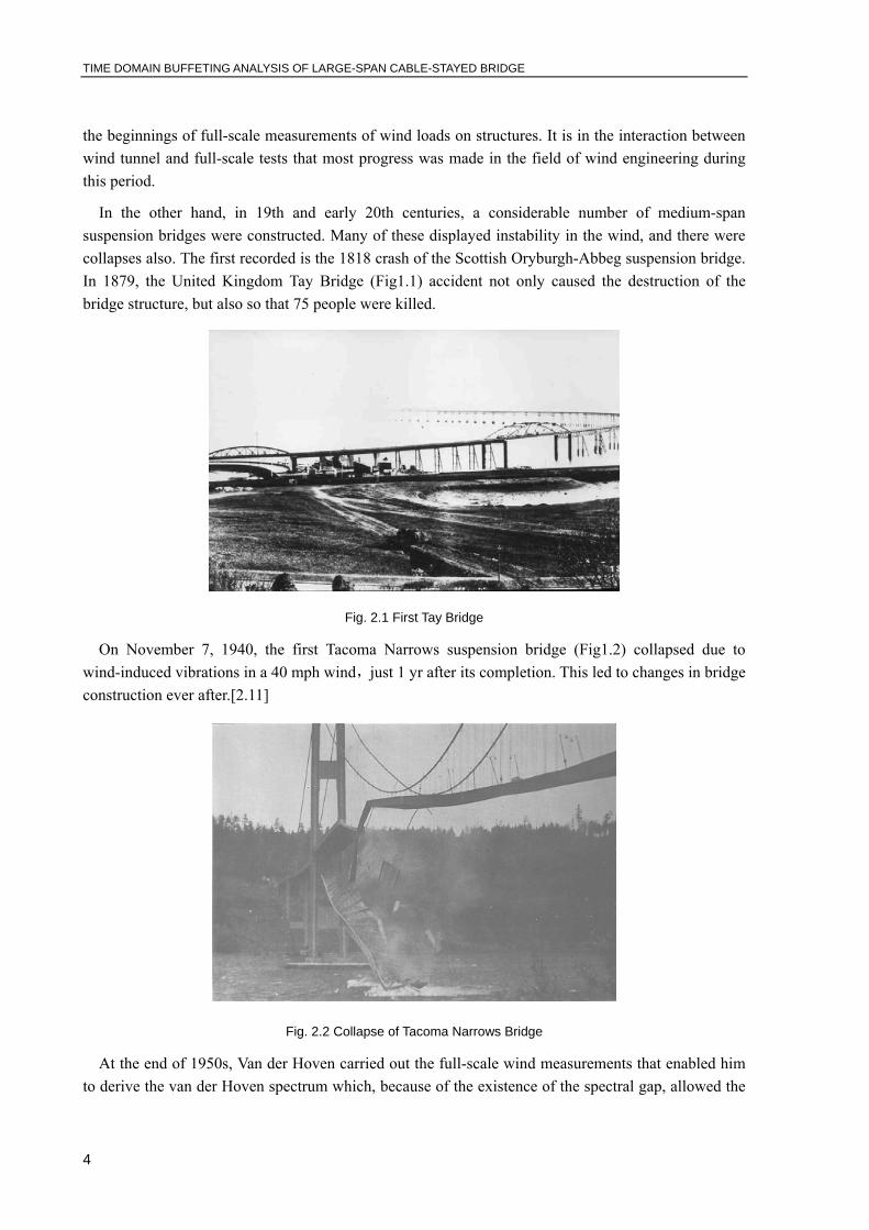
In the other hand, in 19th and early 20th centuries, a considerable number of medium-span suspension bridges were constructed. Many of these displayed instability in the wind, and there were collapses also. The first recorded is the 1818 crash of the Scottish Oryburgh-Abbeg suspension bridge. In 1879, the United Kingdom Tay Bridge (Fig1.1) accident not only caused the destruction of the bridge structure, but also so that 75 people were killed.
Fig. 2.1 First Tay Bridge
On November 7, 1940, the first Tacoma Narrows suspension bridge (Fig1.2) collapsed due to wind-induced vibrations in a 40 mph wind,just 1 yr after its completion. This led to changes in bridge construction ever after.[2.11]
Fig. 2.2 Collapse of Tacoma Narrows Bridge
At the end of 1950s, Van der Hoven carried out the full-scale wind measurements that enabled him to derive the van der Hoven spectrum which, because of the existence of the spectral gap, allowed the

TIME DOMAIN BUFFETING ANALYSIS OF LARGE-SPAN CABLE-STAYED BRIDGE
5
concepts of independent small and large scale wind fluctuations to be formulated, which is of fundamental importance to the developments that followed over the coming decades [2.1].
In the following 20 years, between 1960 and 1980, because of the economic development and the white heat of technology, large-span bridges and other large infrastructure projects were constructed. As the spans increase, wind actions become more critical in bridge design. During this period computer technology began to develop at an accelerating pace, and there were massive developments in the design of scientific instruments and in data acquisition technology.
During this period, there were of course many others involved in the development of the discipline, Davenport play a major role that cannot be over emphasized. In 1961, Alan Davenport elucidated the concept of the wind loading chain, which gave a conceptual framework to the study of wind effects on structures [2.2]. His concept of the wind loading chain, which he applied in the frequency domain, led to a range of spectral methods for calculating the loads and displacements of high rise buildings, bridges, etc. These have become very widely used throughout the discipline, and indeed have become the dominant class of analytical method, although by their nature they implicitly assume linear structural behavior.
These decades saw the development of the boundary layer wind tunnel from an essentially research tool, into a reliable and robust tool for commercial design purposes, with the increasing realization of the need to model the turbulence spectrum as accurately as possible and with the routine use of small pressure transducers with carnivalves, and the introduction of the base balance techniques. Techniques for the measurement and prediction of atmospheric pollutants also advanced rapidly, and in 1961 Pasquil developed his classification of atmospheric stability that was to remain in use for many decades. Around the world a number of ground breaking full-scale experiments took place—the Aylesbury house experiment and the mobile home measurements in the USA. And a significant number of codes were developed by National Standards Organizations—for example the updated UK code (British Standards Institution, 1972) and the Australian Code (Standards Association of Australia, 1973 Standards Association of Australia, 1973).
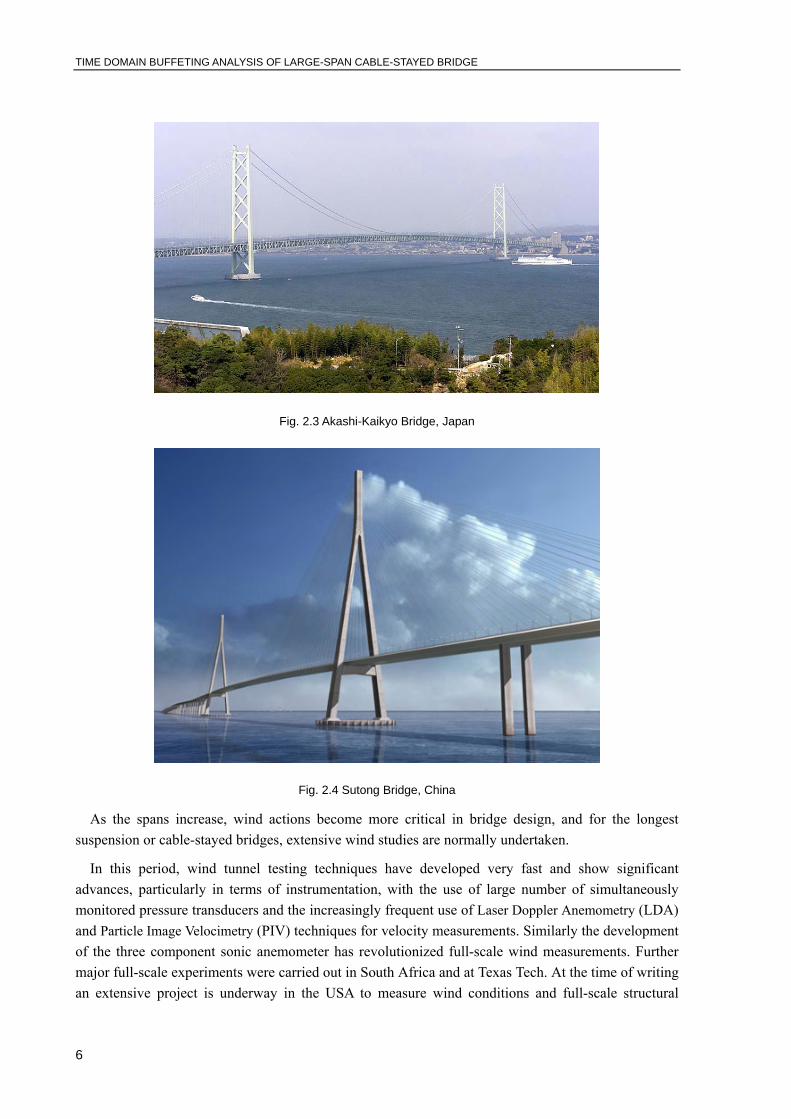
As the time comes to the contemporary period, the spans of the long-span suspension and cable-stayed bridges have been extended to new limits. The longest span bridge in the world is the suspension across the Akashi-Kaikyo Straits in Japan (Fig. 2.3), which has and overall length of 3910 m, with a main span of 1991 m. The design of this bridge was dominated by its aerodynamic characteristics. The longest span cable-stayed bridge is the Sutong Bridge in China, with a overall length of 32.4 km , and a main span of 1088 m (Fig. 2.4).
TIME DOMAIN BUFFETING ANALYSIS OF LARGE-SPAN CABLE-STAYED BRIDGE
6
Fig. 2.3 Akashi-Kaikyo Bridge, Japan
Fig. 2.4 Sutong Bridge, China
As the spans increase, wind actions become more critical in bridge design, and for the longest suspension or cable-stayed bridges, extensive wind studies are normally undertaken.
In this period, wind tunnel testing techniques have developed very fast and show significant advances, particularly in terms of instrumentation, with the use of large number of simultaneously monitored pressure transducers and the increasingly frequent use of Laser Doppler Anemometry (LDA) and Particle Image Velocimetry (PIV) techniques for velocity measurements. Similarly the development of the three component sonic anemometer has revolutionized full-scale wind measurements. Further major full-scale experiments were carried out in South Africa and at Texas Tech. At the time of writing an extensive project is underway in the USA to measure wind conditions and full-scale structural

TIME DOMAIN BUFFETING ANALYSIS OF LARGE-SPAN CABLE-STAYED BRIDGE
7
loading during hurricanes, which should yield a very considerable quantity of information that will be of significant use in design. All these developments have of course been underpinned by the rapid growth in IT techniques and computer power which makes high-speed data acquisition and the analysis of large amounts of experimental data possible. It has also led to the increasing use of what is now the fourth fundamental tool of wind engineering—Computational Fluid Dynamics (CFD) techniques. Computational fluid dynamics has progressed immensely over the past two decades–through the use of inviscid panel methods; then simple k–ε techniques, which were afterwards refined in various ways to make them more suitable for wind engineering application; and now increasingly through unsteady flow methods such as Lager Eddy Simulation (LES), Detached Eddy Simulation (DES) and discrete vortex modeling. For a full review of CFD developments in Wind Engineering, see Murakami and Mochida (1999) [2.3]. The last 20 years have also been extremely busy in terms of code development and revision across the world. These are well summarized in the recent series of papers produced by the IAWE Codification Initiative [2.4]. In conceptual terms the period has seen an increasing application of modern analytical methods to wind engineering—particularly advanced probabilistic techniques, wavelet analysis, orthogonal decomposition, etc.[2.5]. Of particular significance has been the gradual trend towards using time domain methods in the design process. This will be discussed further below.
2.2 Research methods of bridge wind engineering
The modern analysis process of bridge wind engineering needs the use of a variety of theoretical, experimental and numerical methods.
2.2.1 Theoretical analysis
In the field of wind-excited vibration of bridges, A.G Davenport studied the analysis method of buffeting response of suspension bridges early in 1961. Based on the single-mode method (i.e. SRSS method) established by Davenport, R.H.Scanlan [2.8] [2.9] and R.H.Gade(1977) [2.10] accounted for the effect of the self-excited forces by introducing the aerodynamic derivatives, previously used by them in the flutter research, into the mixed time-frequency domain equations of motion, and took the correlation formula for the fluctuation wind-speed spectrum as the correlation formula for the aerodynamic-force power spectrum. As the aerodynamic derivatives and wind-speed spectrum are both frequency domain functions obtained from direct measurements, the application of frequency domain methods in the buffeting analysis has been regarded as a natural selection. The linear flutter theory based on Scanlan’s aerodynamic derivatives is not only readily acceptable by engineers, but is also backed up by a great deal of experimental results. Therefore it has been the prevailing means for bridge designs up to date.
2.2.2 Experimental method
Although the science of theoretical fluid mechanics is well developed and computational methods

TIME DOMAIN BUFFETING ANALYSIS OF LARGE-SPAN CABLE-STAYED BRIDGE
8
are experiencing rapid growth in the area, it remains necessary to perform physical experiments to gain needed in sights into many complex effects associated with fluid flow. This is the well-established field of aeronautics, for which wind tunnels were first developed and to an even greater extent, in the practical study of bridges that stand in the earth’s boundary near-surface atmospheric layer.
There are two kinds of wind tunnel model: full model and sectional model. The full model is a reduced scale geometric facsimile of the entire prototype bridge that includes all structural elements, the towers, the suspension cables, the road deck and the road deck hangers. For dynamic studies, it is necessary, as well, to model the mass, the mass distribution and the elastic characteristics of the prototype according to well-established scaling principles. And rather than model the complete bridge, the aerodynamics of the bridge road deck can be studied by constructing a model that represents a short, mid-span section of the deck. The model spans the test section and is supported rigidly at the wails if force measurements are to be made or is mounted on pairs of springs for dynamic measurements (Fig. 2.6) in which case the mass, the mass distribution and the elastic properties must be modelled according to scaling criteria as is done with the full model. The bending mode natural frequency is controlled by the spring stiffness and the ratio of the bending to torsional mode frequencies is controlled by the spacing between the pairs of springs. If necessary the horizontal stiffness can be modeled by the addition of a spring constraint in the lateral direction.
Fig.2.5 Full model
There are many advantages in wind tunnel testing techniques for studying wind effects on bridges, but many critical phenomena can still only be revealed by full-scale experiments. It has been recognized that the most reliable evaluations of dynamic characteristics and wind effects are obtained from experimental measurements of a prototype bridge. In fact, measurements of wind effects on prototype structures are very useful to improve the understanding of wind-resistant structural design. Meanwhile, the experimental results can also be used to examine the adequacy of wind tunnel test techniques and to refine the numerical models for structural analysis.

TIME DOMAIN BUFFETING ANALYSIS OF LARGE-SPAN CABLE-STAYED BRIDGE
9
Fig.2.6 Sectional model
2.2.3 Numerical methods
Furthermore, recently, the computational fluid dynamics (CFD) technique hare gradually become a popular tool for engineers and has been widely used for the prediction of wind pressures and wind forces on various buildings and structures. Now, it can be concluded that in case of very large 3D computations with a large number of grid points, the aerodynamic characteristics for a simple shape can be successfully simulated with satisfactory accuracy in the limitation of the averaged physical quantities, such as the drag and the lift coefficients. While, the spatial correlation characteristics is still difficult for computational prediction because the flow structures with high frequency have a important role to determine the values.
2.3 Cable-stayed bridges
A typical cable stayed bridge is a continuous girder with one or more towers erected above piers in the middle of the span. From these towers, cables stretch down diagonally (usually to both sides) and support the girder. Cable-stayed bridges carry the vertical main-span loads by nearly straight diagonal cables in tension. The towers transfer the cable forces to the foundations through vertical compression. The tensile forces in the cables also put the deck into horizontal compression. The towers form the primary load-bearing structure. A cantilever approach is often used for support of the bridge deck near the towers, but areas further from them are supported by cables running directly to the towers. This has a disadvantage, compared to suspension bridges. The cables pull to the sides as opposed to directly up, requiring the bridge deck to be stronger to resist the resulting horizontal compression loads. But has the advantage of not requiring firm anchorages to resist a horizontal pull of the cables, as in the suspension bridge. All static horizontal forces are balanced so that the supporting tower does not tend to tilt or slide, needing only to resist such forces from the live loads.
Key advantages of the cable-stayed form are as follows:
• much greater stiffness than the suspension bridge, so that deformations of the deck under live loads are reduced
TIME DOMAIN BUFFETING ANALYSIS OF LARGE-SPAN CABLE-STAYED BRIDGE
10
• can be constructed by cantilevering out from the tower - the cables act both as temporary and permanent supports to the bridge deck
• for a symmetrical bridge (i.e. spans on either side of the tower are the same), the horizontal forces balance and large ground anchorages are not required
There are two major classes of cable-stayed bridges: In a harp design, the cables are made nearly parallel by attaching cables to various points on the tower(s) so that the height of attachment of each cable on the tower is similar to the distance from the tower along the roadway to its lower attachment. In a fan design, the cables all connect to or pass over the top of the tower(s).
The cable-stay design is the optimum bridge for a span length between that of cantilever bridges and suspension bridges. Within this range of span lengths a suspension bridge would require a great deal more cable, while a full cantilever bridge would require considerably more material and be substantially heavier. Of course, such assertions are not absolute for all cases.
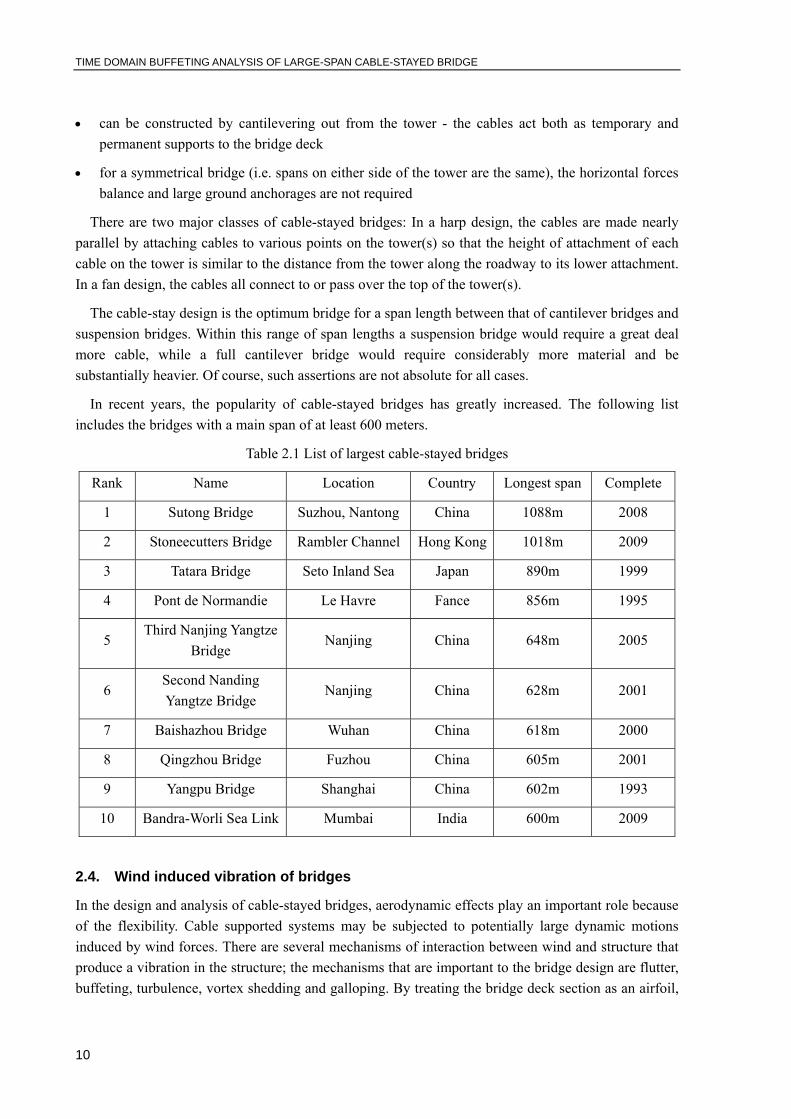
In recent years, the popularity of cable-stayed bridges has greatly increased. The following list includes the bridges with a main span of at least 600 meters.
Table 2.1 List of largest cable-stayed bridges
Rank Name Location Country Longest span Complete
1 Sutong Bridge Suzhou, Nantong China 1088m 2008
2 Stoneecutters Bridge Rambler Channel Hong Kong 1018m 2009
3 Tatara Bridge Seto Inland Sea Japan 890m 1999
4 Pont de Normandie Le Havre Fance 856m 1995
5 Third Nanjing Yangtze
Bridge Nanjing China 648m 2005
6 Second Nanding Yangtze Bridge
Nanjing China 628m 2001
7 Baishazhou Bridge Wuhan China 618m 2000
8 Qingzhou Bridge Fuzhou China 605m 2001
9 Yangpu Bridge Shanghai China 602m 1993
10 Bandra-Worli Sea Link Mumbai India 600m 2009
2.4. Wind induced vibration of bridges
In the design and analysis of cable-stayed bridges, aerodynamic effects play an important role because of the flexibility. Cable supported systems may be subjected to potentially large dynamic motions induced by wind forces. There are several mechanisms of interaction between wind and structure that produce a vibration in the structure; the mechanisms that are important to the bridge design are flutter, buffeting, turbulence, vortex shedding and galloping. By treating the bridge deck section as an airfoil,

TIME DOMAIN BUFFETING ANALYSIS OF LARGE-SPAN CABLE-STAYED BRIDGE
11
the research and knowledge of aeronautics and aerodynamics were brought to bear on the bridge problem. [2.10]
2.4.1. Flutter
Suspension and cable stayed bridges are long slender flexible structures which have potential to be susceptible to a variety of types of wind induced vibrations, the most serious of which is the aerodynamic instability known as flutter. At certain wind speeds aerodynamic forces acting on the deck are of such a nature so as to feed energy into for oscillation structure, so increasing the vibration amplitudes, sometimes to extreme levels where the basic safety of the bridge is threatened. The wind speed at which flutter occurs for completed bridges depends largely on its natural frequencies in vertical blending and torsion, and on the shape of the deck section which determines the aerodynamic forces acting. The Tacoma Narrows Bridge collapsed because of the flutter phenomenon [2.11]. For flutter stability, the lowest wind velocity inducing flutter instability of a bridge must exceed the maximum design wind velocity of that bridge.
2.4.2. Buffeting
Buffeting is defined as the unsteady loading of a structure by velocity fluctuations in the oncoming flow. It causes irregular motions in the bridge structure. The bridge response to buffeting depends on the turbulence intensity, shape of the structural elements and its natural frequencies. Buffeting does not usually endanger the safety of the structure, but can result in discomfort for the users and lead to fatigue of structural elements.
2.4.3. Vortex shedding
Vortex shedding is an unsteady flow that takes place in special flow velocities (according to the size and shape of the cylindrical body). In the flow, vortices are created at the back of the body and detach periodically from either side of the body.
Vortex shedding is caused when a fluid flows past a blunt object. The fluid flow past the object creates alternating low-pressure vortices on the downstream side of the object. The object will tend to move toward the low-pressure zone.
Eventually, if the frequency of vortex shedding matches the resonance frequency of the structure, the structure will begin to resona lock-in and the structure's movement can become self-sustaining. Tall chimneys constructed of thin-walled steel tube can be sufficiently flexible that, in air flow with a speed in the critical range, vortex shedding can drive the chimney into violent oscillations that can lead to fatigue and also collapse of the chimney. These chimneys can be protected from this phenomenon by installing a series of fences at the top and running down the exterior of the chimney for approximately 30% of its length. The fences are usually located in a helical pattern. The fences prevent strong vortex shedding with low separation frequencies.
TIME DOMAIN BUFFETING ANALYSIS OF LARGE-SPAN CABLE-STAYED BRIDGE
12
Vortex shedding was one of the causes proposed for the failure of the original Tacoma Narrows Bridge (Galloping Gertie) in 1940, but was rejected because the frequency of the vortex shedding did not match that of the bridge. The bridge actually failed by aeroelastic flutter [2.11].A thrill ride, "Vertigo" at Cedar Point in Sandusky, Ohio suffered vortex shedding during the winter of 2001, causing one of the three towers to collapse. The rode was closed for the winter at the time. [2.12]
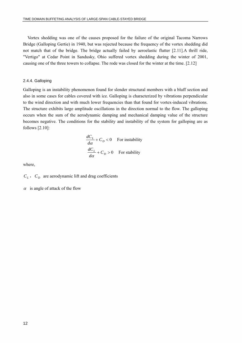
2.4.4. Galloping
Galloping is an instability phenomenon found for slender structural members with a bluff section and also in some cases for cables covered with ice. Galloping is characterized by vibrations perpendicular to the wind direction and with much lower frequencies than that found for vortex-induced vibrations. The structure exhibits large amplitude oscillations in the direction normal to the flow. The galloping occurs when the sum of the aerodynamic damping and mechanical damping value of the structure becomes negative. The conditions for the stability and instability of the system for galloping are as follows [2.10]:
0<+ DL C
ddCα
For instability
0>+ DL C
ddCα
For stability
where,
LC , DC are aerodynamic lift and drag coefficients
α is angle of attack of the flow
TIME DOMAIN BUFFETING ANALYSIS OF LARGE-SPAN CABLE-STAYED BRIDGE
13
3 CHARACTERISTICS OF WIND FIELD
3.1. Introduction
Wind is the motion of air with respect to the surface of the earth, and is fundamentally caused by variable solar heating of the earth’s atmosphere. The longitudinal, vertical and transverse components of the time dependent wind velocity vector at a given location can be expressed as a sum of a constant term and a time dependent function with zero mean:
)()( tuUtU += (3.1a)
)()( tvtV = (3.1b)
)()( twtW = (3.1c)
3.2 Mean wind velocity profiles
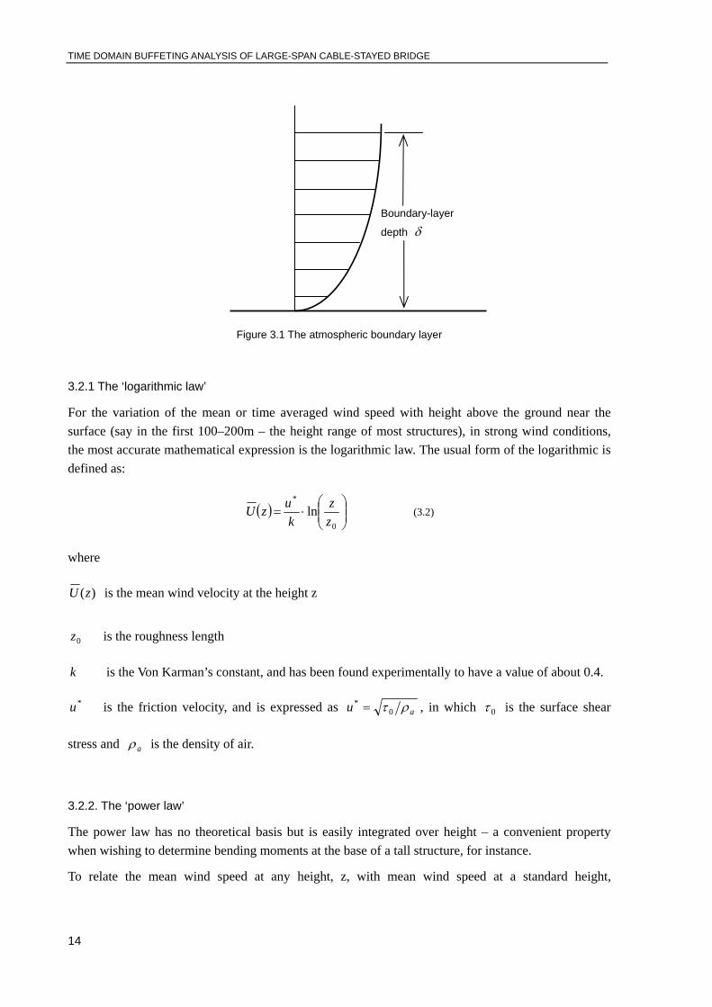
The surface of the earth exerts upon the moving air a horizontal drag force the effect of which is to retard the flow (Fig.3.1). The effect of this force upon the flow decreases as the height above ground increases and becomes negligible above a height δ , known as the height of boundary layer of the atmosphere. The depth of the boundary layer normally ranges in the case of neutrally stratified flows from a few hundred meters to several kilometers, depending upon wind intensity, roughness of terrain, and angle of latitude. Within the boundary layer, the wind speed increases with elevation, and mathematically expressed with ‘logarithmic law’ and ‘power law’.
TIME DOMAIN BUFFETING ANALYSIS OF LARGE-SPAN CABLE-STAYED BRIDGE
14
Figure 3.1 The atmospheric boundary layer
3.2.1 The ‘logarithmic law’
For the variation of the mean or time averaged wind speed with height above the ground near the surface (say in the first 100–200m – the height range of most structures), in strong wind conditions, the most accurate mathematical expression is the logarithmic law. The usual form of the logarithmic is defined as:
( ) ⎟⎟⎠
⎞⎜⎜⎝
⎛⋅=
0
*
lnzz
kuzU (3.2)
where
)(zU is the mean wind velocity at the height z
0z is the roughness length
k is the Von Karman’s constant, and has been found experimentally to have a value of about 0.4.
*u is the friction velocity, and is expressed as au ρτ 0* = , in which 0τ is the surface shear
stress and aρ is the density of air.
3.2.2. The ‘power law’
The power law has no theoretical basis but is easily integrated over height – a convenient property when wishing to determine bending moments at the base of a tall structure, for instance.
To relate the mean wind speed at any height, z, with mean wind speed at a standard height,
Boundary-layer
depth δ
TIME DOMAIN BUFFETING ANALYSIS OF LARGE-SPAN CABLE-STAYED BRIDGE
15
sz (normally, mzs 10= ), the power law can be written [3.1]:
( ) α
⎟⎟⎠
⎞⎜⎜⎝
⎛=
ss zz
UzU (3.3)
The exponent α changes with terrain roughness, and also with the height range, when matched to the
logarithmic law. A relationship that can be used to relate the exponent to the roughness length, 0z , is
as follow:
⎟⎟⎠
⎞⎜⎜⎝
⎛=
0ln
1
zzref
α (3.4)
where refz is a reference height at which the two laws match.
3.3 Wind turbulence
Wind speeds varies randomly with time. This variation is due to the turbulence of the wind flow. Information on the features of atmospheric turbulence is useful in structural engineering. First, rigid structures and members are subjected to time-dependent loads with fluctuations due in part to atmospheric turbulence. Second, flexible structures, such as cable-stayed and suspension bridges, may exhibit resonant amplification effects induced by velocity fluctuations. Third, the aerodynamic behavior of structures depends strongly upon the wind turbulence.
The following features of the atmospheric turbulence are of interest in various applications: the turbulence intensity; the integral scales of turbulent velocity fluctuations; the spectra of turbulent velocity fluctuations; and the cross-spectra of turbulent velocity fluctuations.
3.3.1 Turbulence intensity
The simplest descriptor of atmospheric turbulence is the turbulence intensity. The ratio of the standard deviation of each fluctuating component to the mean value is known as the turbulence intensity of that
component. Let ( )zu denote the velocity fluctuation parallel to the direction of the mean speed. The
longitudinal turbulence intensity is defined as
( ) ( ) ( )zUzzI uu /σ= (3.5)
TIME DOMAIN BUFFETING ANALYSIS OF LARGE-SPAN CABLE-STAYED BRIDGE
16
where ( )zU is mean wind speed at elevation z and ( )zσ is the standard derivation of ( )zu . Vertical
and lateral turbulence intensity may be similarly defined.
Near the ground strong wind produced by large scale depression systems, measurements have found
that the standard deviation of longitudinal wind velocity, uσ is equal to *5.2 u to a good
approximation, where *u is the friction velocity. Then the turbulence intensity, uI , is given as
follow:
( ) ( ) ( )00*
*
/ln1
/ln4.0/5.2
zzzzuu
Iu == (3.6)
Thus the turbulence intensity is simply related to the surface roughness, as measured by the
roughness length, 0z .
The lateral and vertical turbulence components are generally lower in magnitude than the corresponding longitudinal value. However, for well-developed boundary layer winds, simple
relationships between standard deviation of lateral velocity, vσ , is equal to *2.2 u , and for the
vertical component, wσ is given approximately by 1.3 to *4.1 u . Then vI and wI can be derived:
( )0/ln88.0
zzI v ≅ (3.7)
( )0/ln55.0
zzI w ≅ (3.8)
3.3.2. Integral Scales of Turbulence
Integral scales of turbulence represent the average size of the turbulent eddy of the flow. There are altogether nine integral scales of turbulence, corresponding to three dimensions of the eddies associated with the longitudinal, transverse, and vertical components of the fluctuating velocity, u, v and w. For instance, Lu
x, Luy and Lu
z are respectively, measures of the average longitudinal, transverse and vertical size of the eddies related with the longitudinal velocity fluctuations. Mathematically, the longitudinal integral scales of turbulence should be defined as:
( )dxxRL uuu
xu ∫
∞=
02 21
1σ
(3.9)
TIME DOMAIN BUFFETING ANALYSIS OF LARGE-SPAN CABLE-STAYED BRIDGE
17
where x is the direction in witch the fluctuation is measured and of the longitudinal velocity, and
( )xR uu 21is the cross correlation function of the longitudinal velocity components.
3.3.3 Spectra of longitudinal velocity fluctuations
To describe the probabilities distribution of turbulence with frequency, a function called the spectral density usually abbreviated to ‘spectrum’, is used. It is defined so that the contribution to the variance
( 2uσ , or square of the standard deviation), in the range of frequencies from n to n+dn, is given by
dnnSu ⋅)( , where )(nSu is the spectral density function for u(t). Then integration over all
frequencies,
∫∞
=0
2 )( dnnSuuσ (3.10)
There are many mathematical forms that have been used for )(nSu for structural design purposes.
In Eurocode 1 [3.2] wind distribution over frequencies is expressed by the non-dimensional power
spectral, ( )nzS L , , which is determined as follows:
( )nzS L , = ( ) ( )( )( ) 352 ,2.101,8.6,
nzfnzfnzSn
L
L
v ⋅+
⋅=
⋅σ
(3.11)
where ( ) ( )( )zv
zLnnzfm
L⋅
=, is a non-dimensional frequency determined by the frequency n=n1,x, the
natural frequency of the structure in Hz, by the mean velocity vm(z) and the turbulence length scale L(z).
The main frequency of the spectrum is n=0, and corresponding peak value is:
( ) ( )m
v
vzL
S⋅
=2
max8.6
0σ
(3.12)
The American code [3.3]Kaimal form:
( )( ) 352 302.101
868.6x
xnSn
v ⋅+
⋅=
⋅σ
(3.13)
TIME DOMAIN BUFFETING ANALYSIS OF LARGE-SPAN CABLE-STAYED BRIDGE
18
in which z
z
v
nLx = ; zv is the mean hourly wind speed at equivalent height, z ( hz 6.0= , h is the
height of the structure). Transform the mean hourly wind speed into 10min mean wind speed:
smvv h /3094.0 110 ==
smv h /91.311 = (3.14)
The main frequency of the spectra is n=0, and corresponding peak value is:
( )z
zv
v
LS
⋅=
2
max
868.60
σ (3.15)
In this study the Davenport (1961) form [3.4] is used:
( )( ) 342
2
210 1
4
x
x
vK
nnS
+= (3.16)
in which 10
1200v
nx = ; n is the frequency and expressed in Hertz; K is a factor relate to the terrain
roughness, varies from 0.003 to 0.03; 10v is the 10min mean wind speed, in meters per second, at
z=10m. Eq.(3.16) was obtained by averaging results of measurements obtained at various heights above ground and does not reflect the dependence of spectra on height.
The corresponding main frequency and peak value are:
Hzvn 410 104550.6 −×=
( ) 10max 1986 vKnS = (3.17)
In Fig.3.2, all these three spectra are shown at a height z=100m, smv /3010 = .
From Figure 3.2, we can find that in American code and Eurocode the spectra of velocity fluctuation are monotonic decreasing and reach the maximum value at the frequency n=0. In Chinese code at n=0, the spectra S(0)=0, and reaches the maximum value at n=0.02Hz (in case of z=100m,
smv /3010 = ). In the low frequency domain the value is smaller than that of American code and
Eurocode, while in high frequency domain the value of the spectra is larger than that of that of American code and Eurocode. The nature frequencies of practical engineering structures are, generally, between 0.10Hz and 5Hz. In this range, the value of Davenport spectra is the largest.

TIME DOMAIN BUFFETING ANALYSIS OF LARGE-SPAN CABLE-STAYED BRIDGE
19
0 0.05 0.1 0.15 0.2 0.25 0.3 0.35 0.4 0.45 0.50
100
200
300
400
500
600
700
800
n (Hz)
S(n
)
Figure 3.2 Comparison of spectra of velocity fluctuation (z=100m, smv /3010 = ) in different codes
3.3.4 Cross-spectra of longitudinal velocity fluctuations
When considering the resonant response of structures to wind, the correlation of wind velocity fluctuations from separated points at different frequencies is important. For example the correlations of vertical velocity fluctuations with span-wise separation at the natural frequencies of vibration of a large-span bridge are important in determining its response to buffeting.
The cross-spectrum of two continuous records is a measure of the degree to which the two records are correlated and is defined as
( ) =nrS crij , ( ) +nrS C
ij , ( )nriS Qij , (3.18)
in which 1−=i . The real and imaginary parts in Eq.3.18 are known as the co-spectrum and the
quadrature spectrum, respectively. The subscripts i and j indicate that the two different points, the distance between which is r.
The coherence function is defined as
( )[ ] ( ) ( )nrqnrcnrCoh ijij ,,, 222 += (3.19)
where
EN1991-1-4.6
ASNI/ASCE7-95
GB5009-2002
TIME DOMAIN BUFFETING ANALYSIS OF LARGE-SPAN CABLE-STAYED BRIDGE
20
( ) ( )[ ]( ) ( )nSnS
nrSnrc
jjii
Cij
ij
22 ,
, = (3.20a)
( ) ( )[ ]( ) ( )nSnS
nrSnrq
jjii
Qij
ij
22 ,
, = (3.20b)
and ( )nSii , ( )nS jj are the spectra of the longitudinal velocity fluctuations at points i and j .
The following expression for the coherence function was proposed by Davenport [3.7]
( ) ( ) ( )⎥⎥⎥
⎦
⎤
⎢⎢⎢
⎣
⎡
+
−+−+−−=
)()(
2exp)(
222222
ji
jizjiyjixij zUzU
zzCyyCxxCfnCoh (3.21)
where ix , iy , iz and jx , jy , jz are the coordinates of point i and j. zyx CCC ,, are
appropriate decay coefficients, normally determined experimentally.
In homogeneous turbulence, the quadrature spectrum can be neglected [3.8]. For engineering purposes, and based on wind tunnel tests, the cross-spectrum is assumed as
)()()()( nCohnSnSnS ijjjiiij ⋅⋅= (3.22)
3.3.5 Spectra and cross-spectra of vertical velocity fluctuations
It was suggested by Panofsky [3.8] that the spectra of vertical fluctuations up to about 50m may be estimated by the formula
( ) ( )
( )
3/52
*
101
36.3,
⎟⎟⎠
⎞⎜⎜⎝
⎛ ⋅+
⋅⋅
=
zUznn
zUzn
UnzSw (3.23)
where
⎟⎟⎠
⎞⎜⎜⎝
⎛ −=
0
*
lgz
zzkvU
d
;
kzHzd /00 −= ;

TIME DOMAIN BUFFETING ANALYSIS OF LARGE-SPAN CABLE-STAYED BRIDGE
21
0H , mean height of building in the field.
According to measurements reported in [3.6], the cross-spectrum of vertical fluctuations at two points, may be written as
( ) ( ) ( )zUynwij enzSnyS /8,, ∆−=∆ (3.24)
where y∆ is the horizontal distance between the two points.

TIME DOMAIN BUFFETING ANALYSIS OF LARGE-SPAN CABLE-STAYED BRIDGE

TIME DOMAIN BUFFETING ANALYSIS OF LARGE-SPAN CABLE-STAYED BRIDGE
23
4 SIMULATION OF STOCHASTIC WIND VELOCITY FIELD ON LARGE-SPAN BRIDGES
4.1. Introduction
With the development of large span bridges, wind effects become more and more prominent; hence, analysis of wind-induced buffeting of long-span bridges is presently considered necessary. The nonlinear responses of long-span bridges can be computed with sufficient accuracy by time-domain analysis. Simulation of the stochastic wind velocity field on a bridge deck appears currently to be the first step in time-domain analysis of nonlinear buffeting.
The fluctuating wind loads, which are related to the shape and height of the structure, are multiple–points random loads and one of the main dominating excitations of large structures in civil engineering. In the study of buffeting analysis of the structure, the wind velocity is indispensably considered, but an accurate wind velocity model usually requires expensive cost through a full ruler observation or a wind tunnel experiment. Therefore, it is significant to study the wind effects simulation by numerical simulation methods.
The AR model was applied widely to forecast the time series in wind engineering, because of its many merits: simple algorithm and rapid calculation; besides, it can consider not only the space dependent characteristic, but also the time dependent characteristic of the wind history, also, those advantages can be facile to implement by computer programming. Though the autoregressive moving average (ARMA) is superior to the AR model [4.1, 4.2, 4.3, 4.4], the parameter estimation for the ARMA model is much more difficult than the AR model [4.5]. Hence, this chapter still concerns with the issues of the AR model while using it to simulate the natural wind velocity processes.
Before 1980, simulation techniques were primarily adopted to forecast single wind history. However, the single wind history could not meet the requirements of the structure with a great number of degrees of freedom.
Iwatani (1982) proposed the use of an AR model (multidimensional AR process) to simulate
TIME DOMAIN BUFFETING ANALYSIS OF LARGE-SPAN CABLE-STAYED BRIDGE
24
multiple wind velocities firstly [4.6]. The author built a FORTRAN program and gave out two examples, simulation of shear flow in the vertical direction and simulation of two-dimensional homogenous flow at many points in the horizontal direction[4.6], to validate the availability of the AR model. Iannuzzi and Spinelli (1987) compared the methods of simulating both single and multiple wind velocities [4.7]. Huang and Chalabi (1995) used an AR model which could produce non-stationary Gaussian random processes to simulate the wind velocity for the greenhouse and adopted a Kalman filter to estimate the parameters of the AR model [4.8]. All these above researchers used algorithms of iteration and recursion which usually result in accumulative errors while calculating the model parameters.
Stathopoulos, Kumar and Mohammadian (1996) established a first-order AR model to simulate the fluctuating wind loads of monoslope roofs with different geometrics [4.9]. Though the first-order AR model was not enough for the complex structures, the study showed that the AR model could be used to analys the wind-induced responses of the engineering structures. Facchini (1996) used a hybrid model to simulate wind velocity and pointed that the AR model could be calculated directly from the spectral densities without solving the Yule-Walker equations, but it needed huge calculation to obtain covariance functions integrated from the spectral densities of the target processes. [4.10]
Li and Dong (2001) introduced a matrix method to determine the parameters of the AR model without the iteration and recursion, which effectively avoided the accumulative errors in the simulation [4.11]. Although the improved method was applied in the simulation of the wind velocity of the double-layer reticulated shell of Chinese National Grand Theater, there was still some incorrectness in reasoning the covariance matrix and some incorrect descriptions of the formula parameters.
Poggi (2003) used an AR model to simulate wind speed in Corsica and compared to the experimental data to check the correction of the simulated wind speed [4.12]. Roy and Fuller (2001) and Kim (2003) discussed the bias of estimators for AR model parameters and evaluated the effects of bias-correction for AR model parameter estimation [4.13, 4.14].
The wind velocity simulated by numerical simulation methods needs to be as close to the real situation as possible and the simulated method ought to be efficient and general. In the past research, though the AR model was constantly improved, it is not enough for the application of the AR model widely. The drawbacks of poor simulated accuracy of the AR model have not been resolved completely yet. Therefore, this chapter attempts to deduce the AR model by matrix form and solves the raised issues of the AR model in simulating the wind velocity of the spatial 3-D fields systematically, and presents the corresponding solving methods whose computing programs are implemented in MATLAB.
4.2. Simulation of stochastic wind velocity field on long span bridges based on auto-regressive (AR) model
The fluctuating wind velocity is a random time series in essence. The basic formula of the wind velocities [ )(tu ] at M spatial points, idealized as stationary Gaussian multivariate stochastic processes,
TIME DOMAIN BUFFETING ANALYSIS OF LARGE-SPAN CABLE-STAYED BRIDGE
25
can be expressed as [4.6, 4.7, 4.11]:
( )[ ] [ ] ( )[ ] ( )[ ]tNtktutup
kk +∆−=∑
=1
ψ (4.1)
where ( )[ ] ( ) ( )[ ]TM tNtNtN ,,1 L= , ( )[ ]Ti tN is the thi normally distributed stochastic process with
zero mean and unit variance, pi ,L,1= is the rank of AR model, and t∆ is the time step of the
series.
The process of the simulation can be realized as follows.
4.2.1. Calculation of coefficient matrix [ ]kψ
After multiplying the two sides of Eq.4.1 by ( )[ ]tjtu ∆− and calculating the expectation, we can get
the following formula:
( )[ ] ( )[ ]{ } [ ] ( )[ ] ( )[ ] ( )[ ] ( )[ ]{ }tjtutNEtjtutktuEtjtutuEp
kk ∆−+
⎪⎭
⎪⎬⎫
⎪⎩
⎪⎨⎧
∆−∆−=∆− ∑=1
ψ (4.2)
Since the covariance between stochastic process ( )tu and ( )tjtu ∆− can be expressed as
( ) ( ) ( )[ ]{ } ( ) ( )[ ]{ }[ ] ( ) ( )[ ]tjtutuEtjtuEtjtutuEtuEtjRu ∆−=∆−−∆−−=∆ , and the stochastic process
( )tN is independent to stochastic wind velocity ( )tu , then, the relationship between the covariance
( )tjRu ∆ and the regressive coefficient [ ]kψ can be written as:
( ) [ ] ( )[ ]∑=
∆−=∆p
kuku tkjRtjR
1
ψ (4.3)
in which pj ,,2,1 L= . After transpose, Eq. (4.3) can be rewritten in the matrix form:
[ ] [ ][ ]ψRR = (4.4)
where
[ ] ( ) ( )[ ]TuuMpM tpRtRR ∆∆=× ,,L ,

TIME DOMAIN BUFFETING ANALYSIS OF LARGE-SPAN CABLE-STAYED BRIDGE
26
[ ] [ ]TTp
TMpM ψψψ ,,1 L=× ,
[ ]( ) ( ) ( )[ ] ( )[ ]( ) ( ) ( )[ ] ( )[ ]
( )[ ] ( )[ ] ( ) ( )( )[ ] ( )[ ] ( ) ( ) ⎥
⎥⎥⎥⎥⎥
⎦
⎤
⎢⎢⎢⎢⎢⎢
⎣
⎡
∆∆−∆−∆∆−∆−
∆−∆−∆∆∆−∆−∆
=×
021032
23120
uuuu
uuuu
uuuu
uuuu
pMpM
RtRtpRtpRtRRtpRtpR
tpRtpRtRtRtpRtpRtRR
R
L
L
MMOMM
L
L
(4.5)
in which
( )[ ]( ) ( )
( ) ( )[ ]
⎥⎥⎥
⎦
⎤
⎢⎢⎢
⎣
⎡
=⎥⎥⎥
⎦
⎤
⎢⎢⎢
⎣
⎡
∆∆
∆∆=∆
MMj
Mj
Mjj
jMMu
Mu
Muu
u
tjRtjR
tjRtjRtjR
ψψ
ψψψ
K
MOM
L
L
MOM
L
1
111
1
111
, (4.6)
According to random vibration theory, the relationship between the power spectral density and the correlation function accords with the Wiener-Khinchin theorem [4.15]:
( ) ( ) ( )dftjffStjR iku
iku ∆⋅⋅=∆ ∫
∞π2cos
0 (4.7)
where f is the frequency, ( )fS iku is the auto-power spectral density if ki = , the cross-power
spectral density if ki ≠ . Mki L,2,1, = , pj L,1= . The study of this term may be simplified by assuming that the imaginary component of the cross-spectrum is negligible for the purposes of the study that is to be carried out:
)()()()( fCohfSfSfS ijjjiiij ⋅⋅= (4.8)
where )( fCohij represents the coherence function of longitudinal fluctuations at points i and j of the
plane orthogonal to the mean wind direction. As described in Chapter 3, the three-dimension expression of the coherence function is:
( ) ( ) ( )⎥⎥⎥
⎦
⎤
⎢⎢⎢
⎣
⎡
+
−+−+−−=
)()(
2exp)(
222222
ji
jizjiyjixij zUzU
zzCyyCxxCffCoh (4.9)
where, zyx CCC ,, are appropriate decay coefficients. In present study, the following values were
adopted: 8=xC (longitude direction), 16=yC (transverse direction), and 10=zC (vertical
direction).

TIME DOMAIN BUFFETING ANALYSIS OF LARGE-SPAN CABLE-STAYED BRIDGE
27
4.2.2. Calculation of the normally distributed random processes ( )tN
The normally distributed random processes ( )tN can be obtained from:
( )[ ] [ ] ( )[ ]tnLtN = (4.10)
where ( )[ ] ( ) ( ) ( )[ ]TM tntntntn ,,, 21 L= , ( )tni is the thi independent normally distributed random
process with zero mean and unit variance, in which Mi L,2,1,= ; [ ]L is from the Cholesky
decomposition of [ ] [ ] [ ]TN LLR = , in which [ ]NR is calculated from the following equation obtained
by multiplying two sides of Eq. (4.1) with ( )[ ] ( ) ( )[ ]TM tututu ,,1 L=
[ ] ( )[ ] [ ] ( )[ ]tkRRR u
p
kkuN ∆−= ∑
=1
0 ψ (4.11)
4.2.3. Calculation of the fluctuating wind velocity
Using the results of Eq. 4.2 and Eq. 4.8, with the presumption of ( ) 0=tu i , while 0<t , Eq. 4.1
can be dispersed and rewritten as
( )[ ]
( )[ ]
( )[ ]
( )
( )⎥⎥⎥
⎦
⎤
⎢⎢⎢
⎣
⎡
∆
∆+
⎥⎥⎥
⎦
⎤
⎢⎢⎢
⎣
⎡
∆−
∆−=
⎥⎥⎥
⎦
⎤
⎢⎢⎢
⎣
⎡
∆
∆
∑= thN
thN
tkhu
tkhu
hu
thu
M
p
k Mk
M
MMM
1
1
11 )(ψ ,
pkh
,,1,2,1,0
L
L
==
(4.12)
in which t∆ is the discrete time step.
4.2.4. Calculation of the final wind velocity
The final wind velocity can be generated by:
( ) ( )tuUtU += (4.13)
where U is the mean component of wind velocity.

TIME DOMAIN BUFFETING ANALYSIS OF LARGE-SPAN CABLE-STAYED BRIDGE
28
4.2.5. Selection of the AR model rank
Iwatani point out that the low rank of the AR model can meet the requirement in general engineering with the permitted error [4.6]. But, for large and complex structures, it is not credible to solve the rank of AR model based on the empirical analysis only. However, much work has already been done and many experimental results have been given. Ref [4.17, 4.18, 4.19] proposed a new method to select the AR model order by translating the n-variate AR model equations into state-space form. Different from those former works ref [4.23] developed a new method of resolving the rank of AR model based on the principle of the AIC (Akaike Information Criterion). The AIC can be expressed as [4.18]
NppAIC 2ln)( 2 += ασ (4.14)
where N is the sample time length, 2ασ is the variance.
With the increasing rank of the AR model initially, the value of the variance 2ασ and )( pAIC
decrease. However, the value of )( pAIC will increase with the rising rank. Hence, 0p is taken as
the best rank of the AR model if it is determined by the formula for a special rank m
( )pAICpAICmp
∑≤≤
=1
0 min)( (4.15)
It is a huge job to calculate the variance 2ασ for a multidimensional sequence. In this study, it is
proposed that the variance 2ασ can be replaced by the absolute of the maximum eigenvalue of the
matrix [ ]NR .
4.2.6. Implementation of the AR model
There are two important points in the implementations of the AR model based on the MATLAB programming: (Fig 4.1) [4.23]
4.2.6.1. Solving the ill-posed Eq. 4.4 resulting from the increasing degrees of freedom of the structure
Eq. 4.4 can be solved by a general iterative method for a structure with a few degree freedoms
However, the large dimension of the coefficient matrix [ ]R , which results from a large number of
degrees of freedom, will make the Eq.4.4 an ill conditioned equation. Therefore the complicated method with better accuracy is needed for resolving the problem. Here, over-relaxation iteration [4.20] is used to calculate the large sparse matrix equation.

TIME DOMAIN BUFFETING ANALYSIS OF LARGE-SPAN CABLE-STAYED BRIDGE
29
The iteration formula of the algorithm is
( )⎥⎥⎦
⎤
⎢⎢⎣
⎡−−+−= ∑ ∑
−
= +=
++1
1 1
11 1i
l
pM
il
kljil
kljilij
ii
kij
Kij rrr
rψψωψωψ (4.16)
where ω is the relaxation factor which controls the convergent rate of the iteration algorithm,
.,...,2,1 Mi = With the condition of positive definite matrix [ ]R , the formula would be convergent
with 21 <<ω . It is suggested that the relaxation factor value should be within the range of 1.01~1.05 in this study.
4.2.6.2. Solving the numerical integral equation 4.7 which contains oscillating function
The integral function of Eq. 4.7 contains the oscillating function ( )tjf ∆⋅⋅π2cos . With the growth
of the variable tjf ∆⋅⋅⋅π2 , the integral function will have more points of zero value on x-axis coordinate. Then a general numerical interpolation can not meet the requirement of accuracy, and neither can the compound integral method. In this study, the Gauss-Lobatto formula improved from the Gauss formula is used to solve the integral of oscillation function. The formula can be expressed as [4.21]
( ) ( ) ( ) ( )∑−
=
−+++=1
2
221
n
k
nnkknu fKxfAbfAafAR ξ (4.17)
where a, b are the end points of each range, nAA ⋅⋅⋅,1 , nK are 1+n parameters.

TIME DOMAIN BUFFETING ANALYSIS OF LARGE-SPAN CABLE-STAYED BRIDGE
30
Fig. 4.1 Flow chart of implementing wind velocity by AR model in MATLAB
4.3. Case study and wind field evaluation
Using those methods mentioned above, one can simulate the wind velocity at four-space points as
shown in Fig 4.2. The parameters used in the simulation are: the roughness length mz 4.00 = , the
Solve Eq. (4.4) by over-relaxation iteration
Calculate matrix [ ]nR by making
use of Eq. (4.9)
Calculate a new
model rank 1p
Unequal to 0p
Obtain coefficient matrix [ ]ψ
Obtain covariance matrix [ ]uR
Input initial parameters: ,,, 100 tvz ∆
coordinates of space points etc
Assume initial rank of the AR model 0p
Solve Eq. (4.7) by Gauss-Lobatto formula
calculate ( )fS iku
Use new model rank [ ]1p
equal to 0p
Calculate matrix [L] in Eq.(4.8) by Cholesky decomposition
Calculate random numbers matrix [n(t)]
Obtain matrix [N(t)]
Calculate wind velocities [v(t)] by Eq.(4.1)
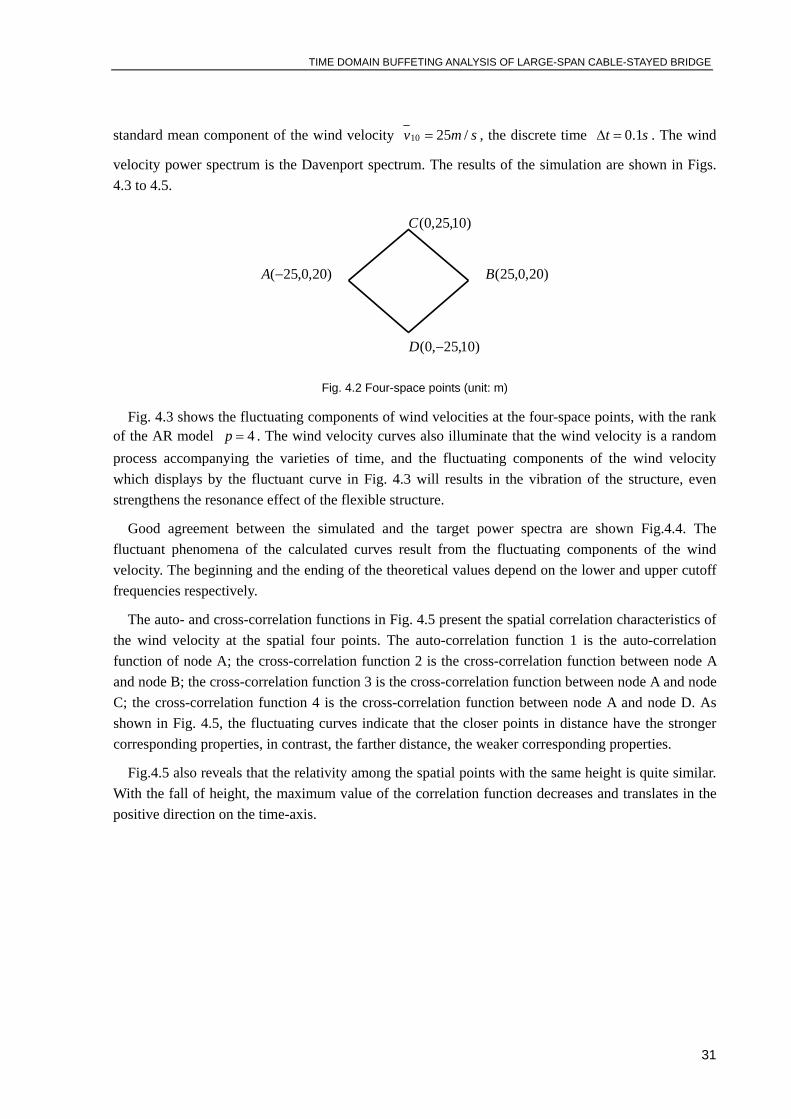
TIME DOMAIN BUFFETING ANALYSIS OF LARGE-SPAN CABLE-STAYED BRIDGE
31
standard mean component of the wind velocity smv /2510 = , the discrete time st 1.0=∆ . The wind
velocity power spectrum is the Davenport spectrum. The results of the simulation are shown in Figs. 4.3 to 4.5.
Fig. 4.2 Four-space points (unit: m)
Fig. 4.3 shows the fluctuating components of wind velocities at the four-space points, with the rank of the AR model 4=p . The wind velocity curves also illuminate that the wind velocity is a random process accompanying the varieties of time, and the fluctuating components of the wind velocity which displays by the fluctuant curve in Fig. 4.3 will results in the vibration of the structure, even strengthens the resonance effect of the flexible structure.
Good agreement between the simulated and the target power spectra are shown Fig.4.4. The fluctuant phenomena of the calculated curves result from the fluctuating components of the wind velocity. The beginning and the ending of the theoretical values depend on the lower and upper cutoff frequencies respectively.
The auto- and cross-correlation functions in Fig. 4.5 present the spatial correlation characteristics of the wind velocity at the spatial four points. The auto-correlation function 1 is the auto-correlation function of node A; the cross-correlation function 2 is the cross-correlation function between node A and node B; the cross-correlation function 3 is the cross-correlation function between node A and node C; the cross-correlation function 4 is the cross-correlation function between node A and node D. As shown in Fig. 4.5, the fluctuating curves indicate that the closer points in distance have the stronger corresponding properties, in contrast, the farther distance, the weaker corresponding properties.
Fig.4.5 also reveals that the relativity among the spatial points with the same height is quite similar. With the fall of height, the maximum value of the correlation function decreases and translates in the positive direction on the time-axis.
)20,0,25(−A
)10,25,0(C
)10,25,0( −D
)20,0,25(B
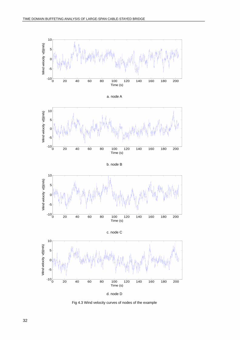
TIME DOMAIN BUFFETING ANALYSIS OF LARGE-SPAN CABLE-STAYED BRIDGE
32
0 20 40 60 80 100 120 140 160 180 200-10
-5
0
5
10
Time (s)
Win
d ve
loci
ty v
(t)(m
/s)
a. node A
0 20 40 60 80 100 120 140 160 180 200-10
-5
0
5
10
Time (s)
Win
d ve
loci
ty v
(t)(m
/s)
b. node B
0 20 40 60 80 100 120 140 160 180 200-10
-5
0
5
10
Time (s)
Win
d ve
loci
ty v
(t)(m
/s)
c. node C
0 20 40 60 80 100 120 140 160 180 200-10
-5
0
5
10
Time (s)
Win
d ve
loci
ty v
(t)(m
/s)
d. node D
Fig 4.3 Wind velocity curves of nodes of the example
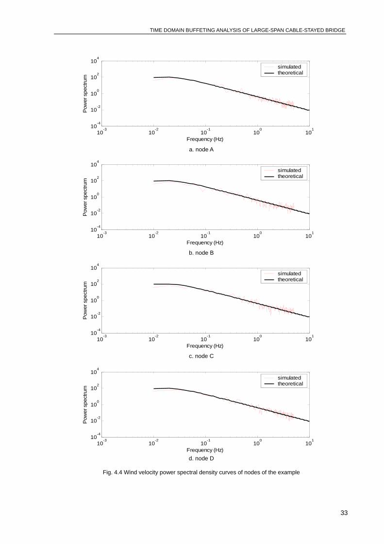
TIME DOMAIN BUFFETING ANALYSIS OF LARGE-SPAN CABLE-STAYED BRIDGE
33
a. node A
b. node B
c. node C
d. node D
Fig. 4.4 Wind velocity power spectral density curves of nodes of the example
10-3
10-2
10-1
100
101
10-4
10-2
100
102
104
Frequency (Hz)
Pow
er s
pect
rum
simulatedtheoretical
10-3
10-2
10-1
100
101
10-4
10-2
100
102
104
Frequency (Hz)
Pow
er s
pect
rum
simulatedtheoretical
10-3
10-2
10-1
100
101
10-4
10-2
100
102
104
Frequency (Hz)
Pow
er s
pect
rum
simulatedtheoretical
10-3
10-2
10-1
100
101
10-4
10-2
100
102
104
Frequency (Hz)
Pow
er s
pect
rum
simulatedtheoretical
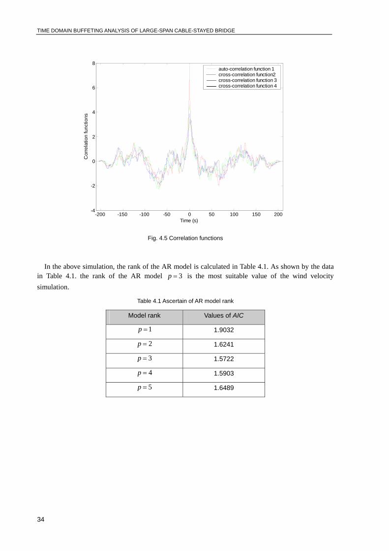
TIME DOMAIN BUFFETING ANALYSIS OF LARGE-SPAN CABLE-STAYED BRIDGE
34
-200 -150 -100 -50 0 50 100 150 200-4
-2
0
2
4
6
8
Time (s)
Cor
rela
tion
func
tions
auto-correlation function 1cross-correlation function2cross-correlation function 3cross-correlation function 4
Fig. 4.5 Correlation functions
In the above simulation, the rank of the AR model is calculated in Table 4.1. As shown by the data in Table 4.1. the rank of the AR model 3=p is the most suitable value of the wind velocity simulation.
Table 4.1 Ascertain of AR model rank
Model rank Values of AIC
1=p 1.9032
2=p 1.6241
3=p 1.5722
4=p 1.5903
5=p 1.6489
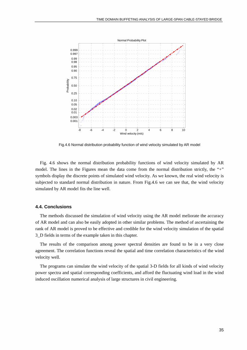
TIME DOMAIN BUFFETING ANALYSIS OF LARGE-SPAN CABLE-STAYED BRIDGE
35
-8 -6 -4 -2 0 2 4 6 8 10
0.0010.003
0.01 0.02 0.05 0.10
0.25
0.50
0.75
0.90 0.95 0.98 0.99
0.9970.999
Wind velocity (m/s)
Pro
babi
lity
Normal Probability Plot
Fig.4.6 Normal distribution probability function of wind velocity simulated by AR model
Fig. 4.6 shows the normal distribution probability functions of wind velocity simulated by AR model. The lines in the Figures mean the data come from the normal distribution strictly, the “+” symbols display the discrete points of simulated wind velocity. As we known, the real wind velocity is subjected to standard normal distribution in nature. From Fig.4.6 we can see that, the wind velocity simulated by AR model fits the line well.
4.4. Conclusions
The methods discussed the simulation of wind velocity using the AR model meliorate the accuracy of AR model and can also be easily adopted in other similar problems. The method of ascertaining the rank of AR model is proved to be effective and credible for the wind velocity simulation of the spatial 3_D fields in terms of the example taken in this chapter.
The results of the comparison among power spectral densities are found to be in a very close agreement. The correlation functions reveal the spatial and time correlation characteristics of the wind velocity well.
The programs can simulate the wind velocity of the spatial 3-D fields for all kinds of wind velocity power spectra and spatial corresponding coefficients, and afford the fluctuating wind load in the wind induced oscillation numerical analysis of large structures in civil engineering.

TIME DOMAIN BUFFETING ANALYSIS OF LARGE-SPAN CABLE-STAYED BRIDGE
37
5 TIME DOMAIN BUFFETING
SIMULATION FOR WIND-BRIDGE
INTERACTION
5.1 Introduction
Buffeting is the vibration motion induced by turbulent wind. As natural wind is not steady but turbulent in character, wind fluctuations in the vertical and horizontal directions are random in space, and thus the wind pressures along the bridges are random in space and time. Depending on the spectral distribution of the pressure vectors, certain modes of vibration on the whole bridge may selectively be excited. In fact, these wind-induced buffeting actions are related not only to wind speed but also to the shape of the cross-section of the bridge deck and the interaction between the bridge and wind motion [5.1]. Significant buffeting may occur for the long-span bridges in strong wind area and may cause serious strength and fatigue problems of structural components and instability of the vehicles traveling on the bridges.
There are mainly two analytical approach for buffeting analysis: time domain approach and frequency domain approach.
To predicate buffeting responses, Davenport [5,3] proposed a quasis-teady method and introduced aerodynamic admittance function, g(w), to consider unsteady effects. Because of the complexity of various cross-section shapes of bridge decks, Scanlan [5.14] suggested that wind tunnel test of bridge
decks be performed to determine the aerodynamic derivatives ( *iA , *
iH , *iP , i=1,…,6) , which are used
for the expression of self-excited force. More recently, Scanlan [1.3] further interpreted the aerodynamic admittance function and gave its inherent relationship with aerodynamic derivatives. These contributions found the basis for conventional buffeting analysis. The dynamic motion equations of bridge decks are generally solved by means of response spectrum theory in frequency domain, which is estimated typically using a mode-by-mode approach that ignores the aerodynamic coupling among modes. In general, the frequency domain approach is restricted to linear structures

TIME DOMAIN BUFFETING ANALYSIS OF LARGE-SPAN CABLE-STAYEDRIDGE
38
excited by the stationary wind loads without aerodynamic nonlinearities. That is a limitation readily acceptable for design considerations under serviceability conditions but not under ultimate strength calculations. In a time domain calculation procedure non-linear load effects or partial structural plastification may be included to provide a better and more comprehensive background for the evaluation of the safety margin at extreme load events. In order to consider the effects of instantaneous relative velocity, effective angle of attack, and structural nonlinearity, the time domain buffeting analysis is necessary.
In time domain simulation, buffeting forces are often considered through the quasi-steady formulation due to its simplicity, without considering unsteady fluid memory effects. To improve that, self-excited force is expressed in terms of convolution integrals between bridge deck motion and impulse response functions, with flutter derivatives identified from wind tunnel test. However, the flutter derivatives and admittance functions are frequency related. As an alternative, a time domain approach using indicial functions can be used [5.18] [5.19] [5.20].
In this thesis both these two approaches for time domain buffeting analysis are introduced.
5.2 Buffeting force
In this section, the forces per unit length acting on a fixed rigid deck section immersed in a turbulent wind flow (Fig. 5.1) are defined. In Fig. 5.1, y0 and z0 are the initial axes of the section. The mean wind velocity U is directed along the x-axis rotated β with respect to x0. The turbulent flow is
characterized by the two fluctuating components ( ) ( )tMutu ,= and ( ) ( )tMwtw ,= , M being a
point representative of the deck section. The mean wind velocity U is assumed to be normal with respect to the longitudinal axis of the deck.
Fig.5.1. Fixed deck section immersed in a turbulent flow
Due to the wind action, surface pressures arise on the contour of the section. The resultant of these
pressures is commonly schematized as a vector ( ) ( ) ( ) ( ){ }Tyxz tMtFtFtF ,,= of (generalized) forces,
where )(tFx is the drag force in the mean wind velocity direction y, )(tFz is the lift force in the
direction z perpendicular to the mean wind velocity, and ( )tM y is the torsional moment.
TIME DOMAIN BUFFETING ANALYSIS OF LARGE-SPAN CABLE-STAYED BRIDGE
39
First the validity of the slender body and quasi-steady hypotheses is assumed, then the quasi-steady hypotheses are removed and the aerodynamic admittance functions are introduced when the quasi-steady hypotheses holds.
5.2.1. Slender body and quasi-steady hypotheses
It is assumed that the bridge deck can be considered as a slender body with respect to its longitudinal axis and that the quasi-steady hypothesis holds. Such hypotheses [5.3] [5.5] hold if the characteristic size of the section is small when compared with the turbulence length scale so as to consider the turbulent eddies as perfectly correlated around the body and if the harmonic content of the signature turbulence is located in correspondence with frequencies higher than those characterizing the undisturbed turbulence so that the signature and the undisturbed turbulence can be considered as uncorrelated and the forces due to these two phenomena can be defined separately. Under this circumstance, the forces due to undisturbed turbulence can be defined as a function of turbulence components in one point representative of the section and can be evaluated defining an instantaneous velocity corresponding to the resultant of the mean wind velocity and of the turbulence components.
Holding the two hypotheses previously introduced, and assuming that the turbulence components
are small with respect to the mean wind velocity ( ( ) Utu <<′ and ( ) Utw <<′ ), the forces can be
separated into a mean vector F and a fluctuating part ( )tF ′ :
( ) ( )tFFtF ′+= (5.1)
The mean forces vector is given by:
⎪⎭
⎪⎬
⎫
⎪⎩
⎪⎨
⎧=
M
L
D
BCCC
BUF 2
21 ρ (5.2)
where ρ is the air density, B is a characteristic size of the deck section (usually the deck width),
DC , LC , and MC are the steady coefficients evaluated at the angle of attack β .
In principle, the fluctuating forces should comprehend two contributions, i.e. ( ) ( ) ( )tFtFtF stut +=′ ,
where ( )tFut is due to the undisturbed turbulence and ( )tFst signature turbulence. It is worth
observing that the contribution to buffeting forces associated with signature turbulence effects is usually neglected in the literature and the buffeting forces take only into account the contribution of
the undisturbed turbulence: ( ) ( ) ( )tFtFtF utb ≅=′ .
Based on such hypothesis, the vector of the buffeting forces is commonly expressed as a function of

TIME DOMAIN BUFFETING ANALYSIS OF LARGE-SPAN CABLE-STAYEDRIDGE
40
the turbulence vector ( ) ( ) ( ){ }TtwtutV ,= by [5.21]:
( ) ( ),21 tVUBCtF aeb ′= ρ
⎥⎥⎥
⎦
⎤
⎢⎢⎢
⎣
⎡
′+′−′
=
MM
DLL
LDD
ae
CBBCCCCCCC
C222
, (5.3)
where aeC is the matrix of the aerodynamic coefficients and DC ′ , LC ′ , MC ′ are the derivatives of
the steady coefficients with respect to the attack angle, and B is the deck width.
5.2.2 Aerodynamic admittance functions
Since bridge deck sections are usually very elongated, the characteristic size of the section cannot be considered as small if compared with the length scales of the turbulence components [5.3, 5.5]. Thus, the turbulence field surrounding the section cannot be considered as perfectly correlated and the forces acting on the deck segment derive from an integration of the pressure field around the section. Despite the three-dimensional nature of the problem, span-wise and chord-wise correlations of the turbulent field around the deck are usually treated as independent.
Moreover, since deck sections are not always streamlined and are characterized by low Strouhal numbers, and the signature turbulence involves a harmonic content overlapping with the harmonic content of the undisturbed turbulence. Differently from the case analyzed in last section, the forces arising on the section as a consequence of these two kinds of turbulence cannot be considered separately.
Under these circumstances, the buffeting forces represent the effects of the undisturbed turbulence and of the signature turbulence together, and can be typically expressed as follows [5.2]:
( ) ( ),21 tVUBC
MLD
tF ae
b
b
b
b ′=⎪⎭
⎪⎬
⎫
⎪⎩
⎪⎨
⎧= ρ (5.4a)
( )( )
⎥⎥⎥
⎦
⎤
⎢⎢⎢
⎣
⎡
′+′−′
=
MMwMMu
DLLwLLu
LDDwDDu
ae
CBBCCCCCCC
Cχχ
χχχχ
222
, (5.4b)
where ( ) ( ) ( ){ }TtwtutV ′′=′ , , and Riχ ( wuiMLDR ,;,, == ) are the six complex aerodynamic
admittance functions (CAAFs) which are functions of reduced frequency.
In this study all the aerodynamic admittance functions are assumed to be unit. This assumption may lead to overestimation of the bridge buffeting response.

TIME DOMAIN BUFFETING ANALYSIS OF LARGE-SPAN CABLE-STAYED BRIDGE
41
5.3 Self-excited forces
Let us consider a moving rigid deck section immersed in a laminar wind flow (Fig. 5.2). The wind
flow is characterized by a mean wind velocity U inclined β with respect to the 0x inertial axis of
the section. The mean wind velocity U is assumed to be normal with respect to the longitudinal axis
of the deck. The motion of the section is described by the components ( )tp in the along wind
direction, ( )th in the crosswind direction and the torsional rotation ( )tα , listed by the vector
( ) ( ) ( ) ( ){ }Ttthtptq α,,= . The forces that act upon a body as a consequence of its motion are commonly
called aeroelastic or self-excited forces.
Fig. 5.2 Moving deck section immersed in a laminar flow.
At first the validity of the quasi-steady hypothesis is assumed (Section 5.3.1), then this hypothesis is removed and the flutter derivatives are introduced (Section 5.3.2).
5.3.1. Quasi-steady hypothesis
Let us assume that the quasi-steady hypothesis holds. If this circumstance is verified, the aerodynamic forces on the body depend on its motion at the same time, and are independent of the history of motion at earlier times. More precisely, the forces acting on the section depend on the instantaneous relative velocity between the flow and the body.
Holding the quasi-steady hypothesis, and assuming that the velocities of the deck section are small
with respect to the mean wind velocity ( ( ) Utp <<& , ( ) Uth <<& and ( ) UtR <<α&0 ), the forces acting on
the section can be expressed as the sum of the mean steady forces ( )tF , given by Eq. 5.2, the forces
associated to the signature turbulence ( )tFst and the self-excited or aeroelastic components ( )tFse ,
given by [5.21]:
( ) ( ) ( )tqKtqCtFse 00 −−= & , (5.5a)
h(t) p(t) ( )tα
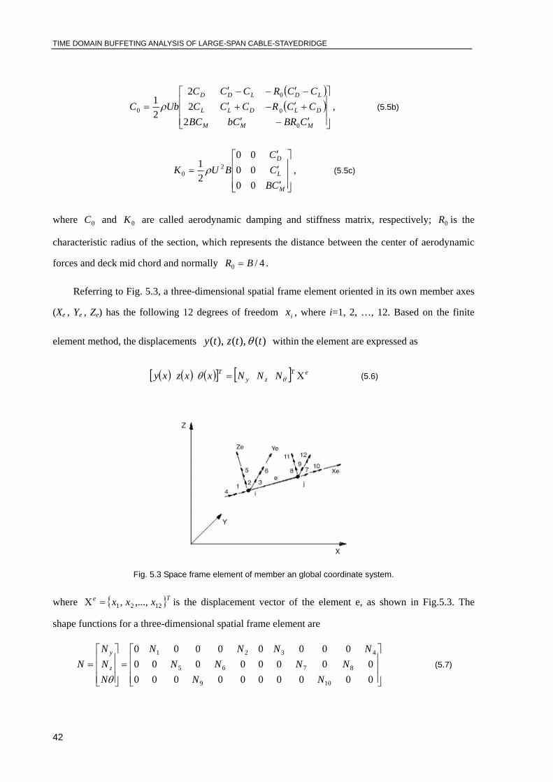
TIME DOMAIN BUFFETING ANALYSIS OF LARGE-SPAN CABLE-STAYEDRIDGE
42
( )( )
⎥⎥⎥
⎦
⎤
⎢⎢⎢
⎣
⎡
′−′+′−+′−′−−′
=
MMM
DLDLL
LDLDD
CBRCbBCCCRCCCCCRCCC
UbC
0
0
0
0
222
21 ρ , (5.5b)
⎥⎥⎥
⎦
⎤
⎢⎢⎢
⎣
⎡
′′′
=
M
L
D
CBCC
BUK000000
21 2
0 ρ , (5.5c)
where 0C and 0K are called aerodynamic damping and stiffness matrix, respectively; 0R is the
characteristic radius of the section, which represents the distance between the center of aerodynamic
forces and deck mid chord and normally 4/0 BR = .
Referring to Fig. 5.3, a three-dimensional spatial frame element oriented in its own member axes
(Xe , Ye , Ze) has the following 12 degrees of freedom ix , where i=1, 2, …, 12. Based on the finite
element method, the displacements )(),(),( ttzty θ within the element are expressed as
( ) ( ) ( )[ ] [ ] eTzy
T NNNxxzxy Χ= θθ (5.6)
Fig. 5.3 Space frame element of member an global coordinate system.
where { }Te xxx 1221 ,...,,=Χ is the displacement vector of the element e, as shown in Fig.5.3. The
shape functions for a three-dimensional spatial frame element are
⎥⎥⎥
⎦
⎤
⎢⎢⎢
⎣
⎡=
⎥⎥⎥
⎦
⎤
⎢⎢⎢
⎣
⎡=
0000
00
00000
00
0000
00
00000
00
10
8
4
7
3
9
6
2
5
1
NN
NN
N
NN
NN
N
NNN
N z
y
θ (5.7)

TIME DOMAIN BUFFETING ANALYSIS OF LARGE-SPAN CABLE-STAYED BRIDGE
43
where
32
51 231 ⎟⎠⎞
⎜⎝⎛+⎟
⎠⎞
⎜⎝⎛−==
Lx
LxNN (5.8a)
32
62 21 ⎟⎠⎞
⎜⎝⎛+⎟
⎠⎞
⎜⎝⎛−==
LxL
LxLNN (5.8b)
32
73 23 ⎟⎠⎞
⎜⎝⎛−⎟
⎠⎞
⎜⎝⎛==
Lx
LxNN (5.8c)
32
84 ⎟⎠⎞
⎜⎝⎛+⎟
⎠⎞
⎜⎝⎛−==
LxL
LxLNN (5.8d)
LxN −= 19 (5.8e)
LxN =10 (5.8f)
where x is the distance from a point within the element to node i and L is the element length.
The equivalent loadings at the element ends are given by the integration of the distributed self-excited forces in Eq. 5.5 over the element length, as
∫=L
aeTe
ae dxPNF0
(5.9)
where
[ ]TTz
Ty
T NNNN θ= , { }Txzyae aeaeaeMFFP = (5.10)
aeyF , aezF and
aexM being self-excited forces in Eq. 5.5. It is straightforward to obtain
eeae
eeae
eae CKF Χ+Χ= (5.11)
where eaeK and e
aeC are the elemental aeroelastic stiffness matrix and aeroelastic damping matrix
for the element e, respectively, and their expressions in the form of consistent formulation are given in the Appendix 1.
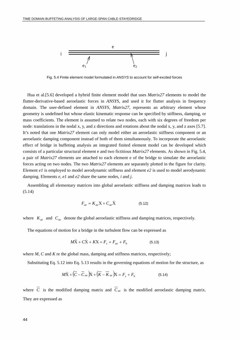
TIME DOMAIN BUFFETING ANALYSIS OF LARGE-SPAN CABLE-STAYEDRIDGE
44
Fig. 5.4 Finite element model formulated in ANSYS to account for self-excited forces
Hua et al.[5.6] developed a hybrid finite element model that uses Matrix27 elements to model the flutter-derivative-based aeroelastic forces in ANSYS, and used it for flutter analysis in frequency domain. The user-defined element in ANSYS, Matrix27, represents an arbitrary element whose geometry is undefined but whose elastic kinematic response can be specified by stiffness, damping, or mass coefficients. The element is assumed to relate two nodes, each with six degrees of freedom per node: translations in the nodal x, y, and z directions and rotations about the nodal x, y, and z axes [5.7]. It’s noted that one Matrix27 element can only model either an aeroelastic stiffness component or an aeroelastic damping component instead of both of them simultaneously. To incorporate the aeroelastic effect of bridge in buffeting analysis an integrated finited element model can be developed which consists of a particular structural element e and two fictitious Matrix27 elements. As shown in Fig. 5.4, a pair of Matrix27 elements are attached to each element e of the bridge to simulate the aeroelastic forces acting on two nodes. The two Matrix27 elements are separately plotted in the figure for clarity. Element e1 is employed to model aerodynamic stiffness and element e2 is used to model aerodynamic damping. Elements e, e1 and e2 share the same nodes, i and j.
Assembling all elementary matrices into global aeroelastic stiffness and damping matrices leads to (5.14)
Χ+Χ= &aeaeae CKF (5.12)
where aeK and aeC denote the global aeroelastic stiffness and damping matrices, respectively.
The equations of motion for a bridge in the turbulent flow can be expressed as
baes FFFKCM ++=Χ+Χ+Χ &&& (5.13)
where M, C and K re the global mass, damping and stiffness matrices, respectively;
Substituting Eq. 5.12 into Eq. 5.13 results in the governing equations of motion for the structure, as
( ) ( ) bsaeae FFKKCCM +=Χ−+Χ−+Χ &&& (5.14)
where C is the modified damping matrix and aeC is the modified aeroelastic damping matrix.
They are expressed as
i j
e1 e2
e

TIME DOMAIN BUFFETING ANALYSIS OF LARGE-SPAN CABLE-STAYED BRIDGE
45
( )aeKKMC −+= βα (5.15a)
aeaeae KCC β−= (5.15b)
where α and β are the proportionality coefficients for Rayleigh damping.
5.3.2 Unsteady buffeting.
Since for bridge deck sections the quasi-steady hypothesis does not usually hold, the forces acting on the section as a consequence of its motion cannot be considered as depending only on the instantaneous motion of the section. Under these circumstances, the self-excited forces are conventionally expressed in the frequency domain as follows:
Self-excited loads are traditionally expressed in the form of indicial functions as suggested by Scanlan [5.8]. However, Lin [5.9] considered that there are some redundancies in the classical formulations. Based on the assumptions that the self-excited loads are generated by linear mechanism, Lin suggested another simple mathematical model for self-excited forces for investigation of the aerodynamic stability of long-span suspension bridges. The self-excited loads are expressed in terms of convolution integrals between bridge deck motion and impulse response functions which is shown to be equivalent to the classical indicial function type representation. Lin's model can be summarized as:
( ) ( ) ( ) ( ) ( ) ( )∫ ∫∞− ∞−−+−=+=
t t
DDphse dttfdtptftDtDtD τατττ αα)( , (5.16a)
( ) ( ) ( ) ( ) ( ) ( )∫ ∫∞− ∞−−+−=+=
t t
LLhhse dttfdthtftLtLtL τατττ αα)( , (5.16b)
( ) ( ) ( ) ( ) ( ) ( )∫ ∫∞− ∞−−+−=+=
t t
MMhhse dttfdthtftMtMtM τατττ αα)( , (5.16c)
where ( )tf Dp , ( )tf Dα , ( )tfLα , ( )tf Lh ( )tf Mα and ( )tfMh are response functions due to unit
impulse displacement α , h and p. From these equations, it is seen that the aerodynamic coupling of the modes is induced by Da(t), La(t) and Mh(t).
Applying the Fourier transform to equations (5.16) and then comparing it with Scanlan's model in terms of aerodynamic derivatives, the relationship between transfer functions and aerodynamic derivatives can be obtained as:
( ) [ ]*2
*3
24 iAABFM += ωρωα , ( ) [ ],*1
*4
23 iAABFMh += ωρω (5.17 a,b)
( ) [ ]*2
*3
23 iHHBFL += ωρωα , ( ) [ ],*1
*4
22 iHHBFMh += ωρω (5.17 c,d)
( ) [ ]*2
*3
23 iPPBFD += ωρωα , ( ) [ ],*1
*4
22 iPPBFDh += ωρω (5.17 e,f)

TIME DOMAIN BUFFETING ANALYSIS OF LARGE-SPAN CABLE-STAYEDRIDGE
46
where A*i and H*
i (i=1,2,3,4) are non-dimensional flutter derivatives obtained by wind tunnel tests on a cross-section of the deck.
As for the introduction of the aerodynamic admittance functions, the definition of the self-excited forces on a deck section owes its origin to the studies made earlier on airfoils and thin-plates. Theodorsen [5.10], applying the potential flow theory, determined analytically the self-excited forces acting on a thin airfoil undergoing crosswind and torsional complex sinusoidal motions. Following this approach, Scanlan and Tomko [5.11] defined the lift and the moment acting on a bridge deck section undergoing crosswind and torsional motions, as functions of suitably defined coefficients, called flutter derivatives. In the case of bridge deck sections, which have to be considered as bluff bodies, the flutter derivatives have to be determined experimentally by wind tunnel tests or by Computational
Fluid Dynamics. Only six flutter derivatives ( *iA , *
iH , i=1,2,3 ) appeared in the original Scanlan and
Tomko [5.11] formulation. With increasing spans, the importance of flutter derivatives associated with the motion in the alongwind direction was emphasized [5.12] and the complete set of the 18 flutter
derivatives ( *iA , *
iH , *iP , i=1,…,6) is considered in recent works[5.22].
From classical air foil theory, the transfer functions may be reasonably approximated by rational functions, specifically for transfer functions of first order linear filters. The transfer functions can, therefore, be expressed as:
⎟⎟⎟⎟⎟
⎠
⎞
⎜⎜⎜⎜⎜
⎝
⎛
⎟⎟⎠
⎞⎜⎜⎝
⎛+
++= ∑=
4
321
2
222
21)(
kkLh
kLhLhLhLh
ni
BUdn
iCCnU
BiCUnFπ
ππρ , (5.18a)
⎟⎟⎟⎟⎟
⎠
⎞
⎜⎜⎜⎜⎜
⎝
⎛
⎟⎟⎠
⎞⎜⎜⎝
⎛+
++= ∑=
4
321
2
222
21)(
kkL
kLLLL
ni
BUdn
iCCnU
BiCUBnFπ
ππρ
α
αααα , (5.18b)
⎟⎟⎟⎟⎟
⎠
⎞
⎜⎜⎜⎜⎜
⎝
⎛
⎟⎟⎠
⎞⎜⎜⎝
⎛+
++= ∑=
4
321
2
222
21)(
kkMh
kMhMhMhMh
ni
BUdn
iCCnU
BiCUBnFπ
ππρ , (5.18c)
⎟⎟⎟⎟⎟
⎠
⎞
⎜⎜⎜⎜⎜
⎝
⎛
⎟⎟⎠
⎞⎜⎜⎝
⎛+
++= ∑=
4
321
22
222
21)(
kkM
kMMMM
ni
BUdn
iCCnU
BiCUBnFπ
ππρ
α
αααα . (5.18d)
Comparing equations (5.17) with equations (5.18), the flutter derivatives can be obtained as

TIME DOMAIN BUFFETING ANALYSIS OF LARGE-SPAN CABLE-STAYED BRIDGE
47
( ) ( )( )⎟
⎟⎠
⎞⎜⎜⎝
⎛
++= ∑
=
4
32222
*1
/11/11
k Lhk
LhkLhkLh
KdKdC
KCK
KH (5.19a)
( ) ( )⎟⎟⎠
⎞⎜⎜⎝
⎛
++= ∑
=
4
322124
/111
k Lhk
LhkLh
KdC
CK
KH (5.19b)
( ) ( )( )⎟
⎟⎠
⎞⎜⎜⎝
⎛
++= ∑
=
4
32222
*2
/11/11
k kL
kLkLL
KdKdC
KCK
KHα
ααα (5.19c)
( ) ( )⎟⎟⎠
⎞⎜⎜⎝
⎛
++= ∑
=
4
32212
*3
/111
k kL
kLL
KdC
CK
KHα
αα (5.19d)
( ) ( )( )⎟
⎟⎠
⎞⎜⎜⎝
⎛
++= ∑
=
4
32222
*1
/11/11
k Mhk
MhkMhkMh
KdKdC
KCK
KA (5.19e)
( ) ( )⎟⎟⎠⎞
⎜⎜⎝
⎛
++= ∑
=
4
32212
*4 /11
1k Mhk
MhkMh Kd
CCK
KA (5.19f)
( ) ( )( )⎟
⎟⎠
⎞⎜⎜⎝
⎛
++= ∑
=
4
32222
*2
/11/11
k kM
kMkMM
KdKdC
KCK
KAα
ααα (5.19g)
( ) ( )⎟⎟⎠
⎞⎜⎜⎝
⎛
++= ∑
=
4
32212
*3
/111
k kM
kMM
KdC
CK
KAα
αα (5.19h)
In the above equations, K is the reduced frequency and is defined asUBK ω
= . The unknown
parameters LhkC , Lhkd , kLC α , kLd α , MhkC , Mhkd , kMC α and kMd α , can be obtained from
least-squares fitting of equations (5.19).
By taking the inverse Fourier transform of the transfer functions, the time domain expression of impulse response functions can be obtained. Substituting these impulse response functions into equation (5.18) yields
( )⎟⎟⎠
⎞⎜⎜⎝
⎛+++= )()()(
21)( 4321
2tLtL
BthC
UB
BthCUBtL hhLhLhh
&ρ (5.20a)
⎟⎠⎞
⎜⎝⎛ +++= )()()()(
21)( 4321
2tLtLtC
UBtCUBtL LL ααααα ααρ & (5.20b)
TIME DOMAIN BUFFETING ANALYSIS OF LARGE-SPAN CABLE-STAYEDRIDGE
48
( )⎟⎟⎠
⎞⎜⎜⎝
⎛+++= )()()(
21)( 4321
22 tMtMBthC
UB
BthCUBtM hhMhMhh
&ρ (5.20c)
⎟⎠⎞
⎜⎝⎛ +++= )()()()(
21)( 4321
22 tMtMtCUBtCUBtM MM ααααα ααρ & (5.20d)
in which, for k=3, 4:
∫∞−
−−=
t tB
Ud
Lhkhk deB
hCtLLhk
ττ τ )()()(&
(5.21a)
( )∫∞−
−−=
t tB
Ud
kLk deCtLkL
ττατ
αα
α )()( & (5.21b)
∫∞−
−−=
t tB
Ud
Mhkhk deB
hCtMMhk
ττ τ )()()(&
(5.21c)
( )∫∞−
−−=
t tB
Ud
kMk deCtMkM
ττατ
αα
α )()( & (5.21d)
Regarding the motion history parts, it can be seen that the items involve convolution integrals of velocities. These series integrals can be summarized as:
( )( )[ ] ( ) ττδτ dtBUdI jt
jij&∫ ∞−
−−= /exp (5.22)
It can be seen that for calculating their values, the integral jI must be evaluated at every time step
jt , which is quite time consuming. Besides the motion history for all elements must be stored, thus
occupying a large computer memory. To tackle these difficulties, a recursive algorithm for evaluating the integral is derived as follows [5.23]:
( )( )[ ] ( )( )[ ] 1111 /exp/exp −−−− ∆−−+−−= jjjijjjij ttBUdIttBUdI δ (5.23)
From the above equation, it can be seen that only the quantities involving 1−jI and 1−jδ at time
1−jt need to be stored for evaluating jI .

TIME DOMAIN BUFFETING ANALYSIS OF LARGE-SPAN CABLE-STAYED BRIDGE
49
5.3.3. Implementation in ANSYS
Because the self-excited forces are dependent on the unknown motion (Eq.20 and Eq.21) they should be calculated iteratively at each time step until the required convergence criterion is satisfied. [5.13]
Step 1: Use ( )1−tu and ( )1−tu& at time t-1 to generate the self-excited forces tseF term in Eq.(5.20).
(i is the number of iteration)
Step 2: by solving Eq.(5.13), the movement of the structure (displacement ( )tu and velocity ( )tu& ) can
be obtained.
Step 3: By substituting ( )tu ( )tu& , which obtained in last step, into Eq.(5.20), the self-excited forces
1+tseF can be obtained.
Step 4: Check convergence of self-excited forces. If convergent, go to the next time step 1+t . If not, repeat step 2-4.

TIME DOMAIN BUFFETING ANALYSIS OF LARGE-SPAN CABLE-STAYEDRIDGE
50
Fig. 4.1 Flow chart of implementing wind velocity by AR model in MATLAB
Solve Eq. (4.4) by over-relaxation iteration
Calculate matrix [ ]nR by making
use of Eq. (4.9)
Calculate a new
model rank 1p
Unequal to 0p
Obtain coefficient matrix [ ]ψ
Obtain covariance matrix [ ]uR
Input initial parameters: ,,, 100 tvz ∆
coordinates of space points etc
Assume initial rank of the AR model 0p
Solve Eq. (4.7) by Gauss-Lobatto formula
calculate ( )fS iku
Use new model rank [ ]1p
equal to 0p
Calculate matrix [L] in Eq.(4.8) by Cholesky decomposition
Calculate random numbers matrix [n(t)]
Obtain matrix [N(t)]
Calculate wind velocities [v(t)] by Eq.(4.1)

TIME DOMAIN BUFFETING ANALYSIS OF LARGE-SPAN CABLE-STAYED BRIDGE
51
6 APPLICATION TO QINGZHOU
BRIDGE
6.1. Bridge description and the main parameters.
The Qingzhou cable-stayed bridge, as shown in Fig. 6.1, is one of the bridges on Luo-Chang Highway over the Min River in Fuzhou, Fujian Province, China. The bridge has a composite-deck system consisting of five spans with an overall length of 1186.34 m (41.13 m + 250 m + 605 m + 250 m + 40.21 m). At the time, its 605 m main span was the longest span length among the completed composite-deck cable-stayed bridges, and ranks the fifth among the all types completed cable-stayed bridges all over the world. The bridge was completed in the year of 2000, but it was officially opened to the traffic in the year of 2002 due to the construction delay of approach spans. Fig. 6.2 shows the schematic plan, elevation and deck cross-section views of the Qingzhou cable-stayed bridge. The bridge, having six lanes, carries two roadways with 29 m wide. The main structural features of the bridge are briefly described as follows.

TIME DOMAIN BUFFETING ANALYSIS OF LARGE-SPAN CABLE-STAYED BRIDGE
52
Fig. 6.1 Qingzhou cable-stayed bridge
The composite-deck system of the bridge has an open-section consisting of two main I-type steel girders, steel floor beams and 25 cm thickness concrete slab. The slender steel girder is 2.45 m high and its maximum plate thickness reaches 80 mm. The ratio of girder height to span length is about 1/202. One steel stringer is designed in the middle of the cross-section. There are in total 257 steel floor beams with a spacing of 4.5 m. The precast concrete slab is connected to the steel girders and floor beams by shear studs.
The two diamond-shaped towers are of reinforced concrete. The height of the towers is 175.5 m
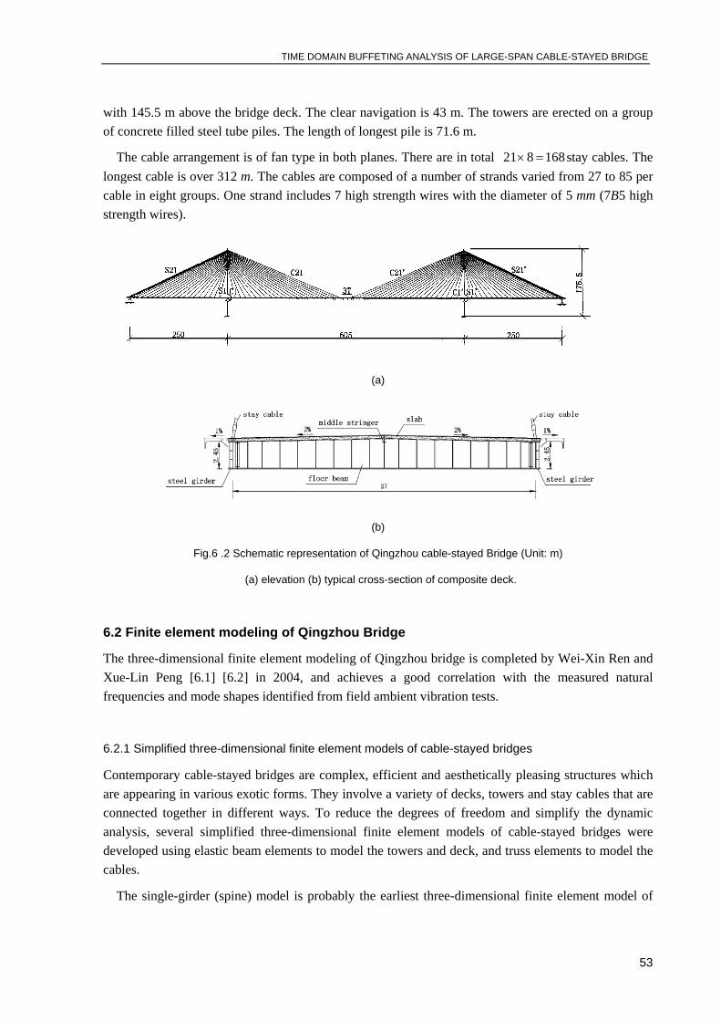
TIME DOMAIN BUFFETING ANALYSIS OF LARGE-SPAN CABLE-STAYED BRIDGE
53
with 145.5 m above the bridge deck. The clear navigation is 43 m. The towers are erected on a group of concrete filled steel tube piles. The length of longest pile is 71.6 m.
The cable arrangement is of fan type in both planes. There are in total 168821 =× stay cables. The longest cable is over 312 m. The cables are composed of a number of strands varied from 27 to 85 per cable in eight groups. One strand includes 7 high strength wires with the diameter of 5 mm (7B5 high strength wires).
(a)
(b)
Fig.6 .2 Schematic representation of Qingzhou cable-stayed Bridge (Unit: m)
(a) elevation (b) typical cross-section of composite deck.
6.2 Finite element modeling of Qingzhou Bridge
The three-dimensional finite element modeling of Qingzhou bridge is completed by Wei-Xin Ren and Xue-Lin Peng [6.1] [6.2] in 2004, and achieves a good correlation with the measured natural frequencies and mode shapes identified from field ambient vibration tests.
6.2.1 Simplified three-dimensional finite element models of cable-stayed bridges
Contemporary cable-stayed bridges are complex, efficient and aesthetically pleasing structures which are appearing in various exotic forms. They involve a variety of decks, towers and stay cables that are connected together in different ways. To reduce the degrees of freedom and simplify the dynamic analysis, several simplified three-dimensional finite element models of cable-stayed bridges were developed using elastic beam elements to model the towers and deck, and truss elements to model the cables.
The single-girder (spine) model is probably the earliest three-dimensional finite element model of

TIME DOMAIN BUFFETING ANALYSIS OF LARGE-SPAN CABLE-STAYED BRIDGE
54
cable-stayed bridges in structural dynamics. The bridge deck was modeled using a single central spine with offset rigid links to accommodate cable anchor points. The deck stiffness was assigned to the spine, and mass (translational and rotational) was assigned to the spine nodes. This simplified model neglects the floor beam stiffness and girder torsional, so it is suitable for a box section girder with relatively large pure torsional stiffness but small torsional stiffness.
To take the torsional stiffness of the bridge deck into account in the single-girder beam element model, Wilson and Gravelle [6.3] presented a Π type model where the deck stiffness and mass were separately treated. Due to the distribution of lumped mass on both sides, the rotation effect of deck mass can be automatically included. This model may produce coupling between torsional and lateral motions of the deck using an equivalent pure torsional stiffness.
For cable-stayed bridges with double cable planes and open-section deck systems, the double-girder model seems more natural. The double-girder beam element model consists of two girders located in each cable plane coupled to floor beams. This model may include part of torsional stiffness through the opposite vertical bending of the two girders. Nazmy and Abdel-Ghaffar [6.7] [6.8] successfully applied the model to the three-dimensional nonlinear earthquake-response analysis of long-span cable-stayed bridge.
The torsional stiffness of the open-section decks is one of the most difficult parameters to estimate in developing a model of cable-stayed bridges. Zhu et al. [6.4] presented a triple-girder beam element model consisting of one central girder and two side girders to include the torsional stiffness properly. If deck stiffness and mass are correctly equalized and distributed to three girders, the torsional stiffness can be effectively considered. The model was verified through a comparison with the measured dynamic results of the Nanpu cable-stayed bridge.
The modeling of deck system is relatively ambiguous by using simplified beam element models. The adequacy of the simplified models is particularly questionable when representing the bridge deck system in the lateral and torsional vibration. The lateral vibration modes may be distorted to some extent if the deck stiffness equivalence is treated improperly. A dynamic study on the composite-deck system of an arch bridge has shown that the first lateral frequency of the triple-girder model is twice that of the double-girder model. Relatively large differences of torsional frequencies were also found between two models. Ren et al.[6.5] verified the stiffness contribution of the concrete slab through finite element analysis and field ambient vibration tests on a steel arch bridge with a composite-deck system. The concrete slab may have lass effect on the vertical bending stiffness, but may be a large contribution to the lateral bending stiffness of the deck. To represent the bridge dynamic behavior well, instead of simplified beam element models, a full three-dimensional finite element model is required with several types of elements such as beam elements, truss elements, shell elements, solid elements and link elements representing different components of cable stayed bridges. Some of them are introduced as follow, assuming the use of ANSYS system [6.6]:
6.2.1.1 BEAM 4
BEAM4 is a uniaxial element with tension, compression, torsion, and bending capabilities (Fig.6.3). The element has six degrees of freedom at each node: translations in the nodal x, y, and z directions and rotations about the nodal x, y, and z axes.
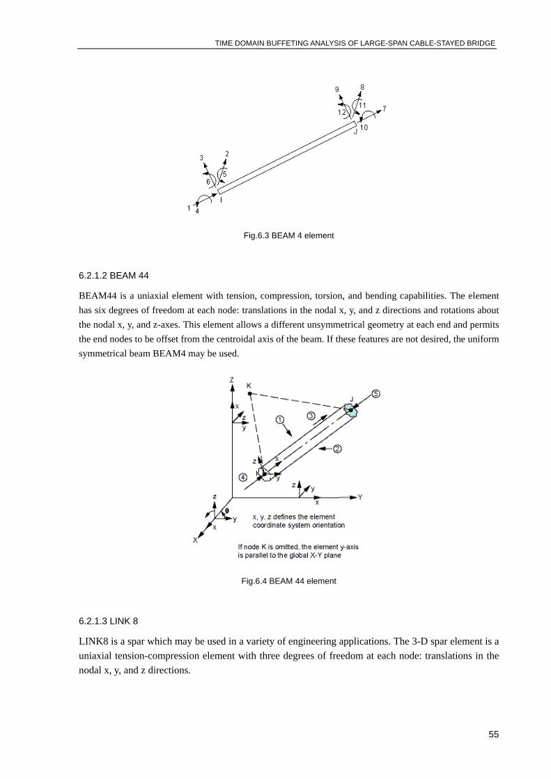
TIME DOMAIN BUFFETING ANALYSIS OF LARGE-SPAN CABLE-STAYED BRIDGE
55
Fig.6.3 BEAM 4 element
6.2.1.2 BEAM 44
BEAM44 is a uniaxial element with tension, compression, torsion, and bending capabilities. The element has six degrees of freedom at each node: translations in the nodal x, y, and z directions and rotations about the nodal x, y, and z-axes. This element allows a different unsymmetrical geometry at each end and permits the end nodes to be offset from the centroidal axis of the beam. If these features are not desired, the uniform symmetrical beam BEAM4 may be used.
Fig.6.4 BEAM 44 element
6.2.1.3 LINK 8
LINK8 is a spar which may be used in a variety of engineering applications. The 3-D spar element is a uniaxial tension-compression element with three degrees of freedom at each node: translations in the nodal x, y, and z directions.

TIME DOMAIN BUFFETING ANALYSIS OF LARGE-SPAN CABLE-STAYED BRIDGE
56
Fig. 6.5 LINK 8 element
iv) LINL 10
LINK10 is a 3-D spar element having the unique feature of a bilinear stiffness matrix resulting in a uniaxial tension-only (or compression-only) element. With the tension-only option, the stiffness is removed if the element goes into compression.
Fig.6.6 Link 10 element
6.2.2 Full three-dimensional finite element modeling of the Qingzhou cable-stayed bridge
Aimed at establishing a baseline finite element model for the long-term health monitoring of the Qingzhou cable-stayed bridge, a full three-dimensional finite model was conceived in ANSYS [6.1] because of the program significant capability to account for the initial cable tension and pre-stressed modal analysis capability.
6.2.2.1 The modeling of each part of bridge
1. Two steel girders and one central stringer are modeled as the 3-D elastic beam elements (BEAM4), since they are the structural members possibly subjected to tension, compression, bending and torsion. There are in total 968 elements of this type.
2. The side spans include T-type concrete beams that are also discreterized by the BEAM4 element that results 499 elements.

TIME DOMAIN BUFFETING ANALYSIS OF LARGE-SPAN CABLE-STAYED BRIDGE
57
3. The floor beams are of variable sections and thus they are modeled by the BEAM44 elements. 554 elements of this type are used in the current model.
4. Towers consist of both equivalent and variable sections so they are discreterized by both BEAM4 and BEAM44 elements with a total number of 140.
5. All piers and platforms are modeled by the solid elements (SOLID45), of which there are 193.
6. The concrete slab is divided into 508 shell elements (SHELL63).
7. 210 concentrated mass elements (MASS21) are used to include the mass of equilibrium blocks, parapet and anchors that are nonstructural members.
8. Modeling of the stay cables is possible in ANSYS by employing the 3-D tension-only truss elements (LINK10), and utilizing its stress-stiffening capability. With this element, the stiffness is removed if the element goes into compression, thus simulating a slack cable. No bending stiffness is included, whereas the pre-tensions of the cables can be incorporated by the initial strains of the element. The stress-stiffening capability is needed for analysis of structures with a low or nonexisting bending stiffness as is the case with cables. The cable sagging effect can be considered with the stress-stiffening capability. The element is nonlinear and requires an iterative solution. Each stay cable is modeled by one element, which results in 168 tension-only truss elements in the model.
6.2.2.2 The modeling of bridge boundary conditions
The modeling of bridge boundary conditions is an important issue in the dynamic analysis. Two types of bridge bearings are used in the Qingzhou cable-stayed bridge. Fixed bearings are applied to Pier 2, while expansion bearings are used for the other piers. In the current model, bridge bearings are modeled by a set of rigid link elements connecting the superstructure and piers.
To simulate the actual behavior, the fixed and expansion bearings are simulated by coupling the corresponding translational and rotational degrees of freedom at both end nodes of the link elements. In addition, there are expansion joints at Pier 0 and Pier 5. Longitudinal springs (COMBINE14) are then applied to account for the restraining action in the longitudinal direction.
6.2.2.3 Material properties of structural members
168 cables are divided into eight groups. Their material and geometric properties are listed in Table 6.1. The basic material properties of other structural members are summarized in Table 6.2.

TIME DOMAIN BUFFETING ANALYSIS OF LARGE-SPAN CABLE-STAYED BRIDGE
58
Table 6.1 Properties of stay cables
Cable No. Number of
strands Area(cm2)
Linear Mass (Kg/m)
E(MPa) ( )MPaσ
C1-C4, S1-S4 27- 15φ 37.80 32.79
C5-C6, S5-S6 34- 15φ 47.59 41.39
C7-C9, S7-S8 37- 15φ 51.79 44.94
C10-C12, S9-S10
43- 15φ 60.19 52.22
C13-C14, S11-S13
48- 15φ 67.19 58.30
C15-C18 55- 15φ 76.99 66.80
C19-C20 73- 15φ 102.19 88.66
C21,S20-S21 85- 15φ 118.93 103.23
51095.1 × 1860
Table 6.2 Material properties of structural members
Materials E(MPa) Volumic mass (Kg/cm3)
Structural members
Steel 51010.2 × 7850 Girders, floor beams, stringer
Concrete C30 41000.3 × 2550 Platform of piers
Concrete C40 41025.3 × 2550 Piers
Concrete C50 41045.3 × 2550 Tower, T-beams
Concrete C60 41060.3 × 2550 Concrete slab
6.2.2.4 Full three-dimensional finite element model of the Qingzhou cable-stayed bridge
The full three-dimensional finite element model of the Qingzhou cable-stayed bridge is shown in Fig. 6.7. The complete model consists of 1840 nodes and 3238 elements resulting in 9193 active degrees of freedom (DOFs). The model represents the bridge in its current as-built configuration and structural properties.

TIME DOMAIN BUFFETING ANALYSIS OF LARGE-SPAN CABLE-STAYED BRIDGE
59

TIME DOMAIN BUFFETING ANALYSIS OF LARGE-SPAN CABLE-STAYED BRIDGE
60
Fig. 6.7 Finite element model of Qingzhou Bridge
6.2.2.5 Initial equilibrium configuration
One of the important features of a large span cable-stayed bridge is that the dead load (self weight) is often dominant. The pre-tensions in the stay cables control the internal force distribution in the deck and towers as well as the bridge alignment. The initial equilibrium configuration of cable-stayed bridges is therefore the equilibrium position due to dead load and tension forces in the stay cables. The initial equilibrium configuration is important in cable-stayed bridges since it is a starting position to perform the succeeding analysis.
In this cable-stayed bridge, the initial deformed equilibrium configuration of the finite element model should be identical to the completed initial geometry alignment of the bridge deck. This can be realized by manipulating the initial tension force in each stay cable that is specified as an input quantity in the cable elements. The design cable tensions are first applied to each stay cable and the
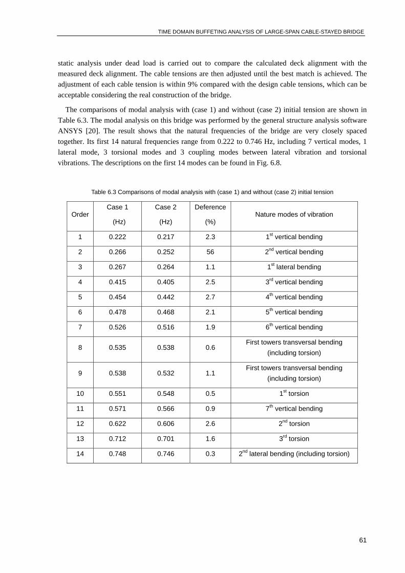
TIME DOMAIN BUFFETING ANALYSIS OF LARGE-SPAN CABLE-STAYED BRIDGE
61
static analysis under dead load is carried out to compare the calculated deck alignment with the measured deck alignment. The cable tensions are then adjusted until the best match is achieved. The adjustment of each cable tension is within 9% compared with the design cable tensions, which can be acceptable considering the real construction of the bridge.
The comparisons of modal analysis with (case 1) and without (case 2) initial tension are shown in Table 6.3. The modal analysis on this bridge was performed by the general structure analysis software ANSYS [20]. The result shows that the natural frequencies of the bridge are very closely spaced together. Its first 14 natural frequencies range from 0.222 to 0.746 Hz, including 7 vertical modes, 1 lateral mode, 3 torsional modes and 3 coupling modes between lateral vibration and torsional vibrations. The descriptions on the first 14 modes can be found in Fig. 6.8.
Table 6.3 Comparisons of modal analysis with (case 1) and without (case 2) initial tension
Order Case 1
(Hz)
Case 2
(Hz)
Deference
(%) Nature modes of vibration
1 0.222 0.217 2.3 1st vertical bending
2 0.266 0.252 56 2nd vertical bending
3 0.267 0.264 1.1 1st lateral bending
4 0.415 0.405 2.5 3rd vertical bending
5 0.454 0.442 2.7 4th vertical bending
6 0.478 0.468 2.1 5th vertical bending
7 0.526 0.516 1.9 6th vertical bending
8 0.535 0.538 0.6 First towers transversal bending
(including torsion)
9 0.538 0.532 1.1 First towers transversal bending
(including torsion)
10 0.551 0.548 0.5 1st torsion
11 0.571 0.566 0.9 7th vertical bending
12 0.622 0.606 2.6 2nd torsion
13 0.712 0.701 1.6 3rd torsion
14 0.748 0.746 0.3 2nd lateral bending (including torsion)

TIME DOMAIN BUFFETING ANALYSIS OF LARGE-SPAN CABLE-STAYED BRIDGE
62
1st vertical bending mode 2nd vertical bending mode
1st lateral bending mode 3rd vertical bending mode
4th vertical bending mode 5th vertical bending mode
6th vertical bending mode First towers transversal bending
(including torsion)

TIME DOMAIN BUFFETING ANALYSIS OF LARGE-SPAN CABLE-STAYED BRIDGE
63
First towers transversal bending 1st torsion mode
(including torsion)
7th vertical bending mod 2nd torsion mode
3rd torsion mode 2nd lateral bending mode
(including torsion)
Fig. 6.8 Typical mode shapes
6.3 Time domain wind velocity generated by auto-regressive method
The wind velocity field on the bridge deck is assumed to be composed of 87 wind velocity waves at 87 different points distributed along the deck of the bridge. According to the original design document, the main data of the bridge and of the time domain wind velocity generation conditions are as follows:
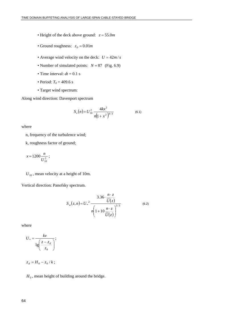
TIME DOMAIN BUFFETING ANALYSIS OF LARGE-SPAN CABLE-STAYED BRIDGE
64
• Height of the deck above ground: mz 0.55=
• Ground roughness: mz 01.00 =
• Average wind velocity on the deck: smU /42=
• Number of simulated points: 87=N (Fig. 6.9)
• Time interval: dt = 0.1 s
• Period: T0 = 409.6 s
• Target wind spectrum:
Along wind direction: Davenport spectrum
( )( ) 3/42
2210
1
4
xn
kxUnSv+
= (6.1)
where
n, frequency of the turbulence wind;
k, roughness factor of ground;
210
1200U
nx = ;
10U , mean velocity at a height of 10m.
Vertical direction: Panofsky spectrum.
( ) ( )
( )
3/52
*
101
36.3,
⎟⎟⎠
⎞⎜⎜⎝
⎛ ⋅+
⋅⋅
=
zUznn
zUzn
UnzSw (6.2)
where
⎟⎟⎠
⎞⎜⎜⎝
⎛ −=
0
*
lgz
zzkvU
d
;
kzHzd /00 −= ;
0H , mean height of building around the bridge.
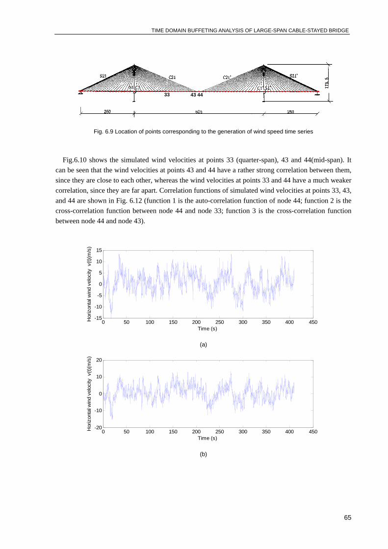
TIME DOMAIN BUFFETING ANALYSIS OF LARGE-SPAN CABLE-STAYED BRIDGE
65
Fig. 6.9 Location of points corresponding to the generation of wind speed time series
Fig.6.10 shows the simulated wind velocities at points 33 (quarter-span), 43 and 44(mid-span). It can be seen that the wind velocities at points 43 and 44 have a rather strong correlation between them, since they are close to each other, whereas the wind velocities at points 33 and 44 have a much weaker correlation, since they are far apart. Correlation functions of simulated wind velocities at points 33, 43, and 44 are shown in Fig. 6.12 (function 1 is the auto-correlation function of node 44; function 2 is the cross-correlation function between node 44 and node 33; function 3 is the cross-correlation function between node 44 and node 43).
0 50 100 150 200 250 300 350 400 450-15
-10
-5
0
5
10
15
Time (s)
Hor
izon
tal w
ind
velo
city
v(t)
(m/s
)
(a)
0 50 100 150 200 250 300 350 400 450-20
-10
0
10
20
Time (s)
Hor
izon
tal w
ind
velo
city
v(t)
(m/s
)
(b)
43 44 33

TIME DOMAIN BUFFETING ANALYSIS OF LARGE-SPAN CABLE-STAYED BRIDGE
66
0 50 100 150 200 250 300 350 400 450-20
-10
0
10
20
Time (s)
Hor
izon
tal w
ind
velo
city
v(t)
(m/s
)
(c)
Fig.6.10 Simulated horizontal wind velocities at point 44(a), 43(b), 33(c)
10-3 10-2 10-1 100 10110-2
100
102
104
Frequency (Hz)
Am
plitu
de
(a)
10-3 10-2 10-1 100 10110-2
100
102
104
Frequency (Hz)
Ampl
itude
(b)
simulatedtheoretical
simulatedtheoretical

TIME DOMAIN BUFFETING ANALYSIS OF LARGE-SPAN CABLE-STAYED BRIDGE
67
10-3 10-2 10-1 100 10110-2
100
102
104
Frequency (Hz)
Am
plitu
de
(c)
Fig. 6.11 Horizontal wind velocity power spectral density curves at point 44(a), 43(b), 33(c)
-400 -300 -200 -100 0 100 200 300 400-5
0
5
10
15
20
Time (s)
Cor
rela
tion
func
tions
auto-correlation function 1 auto-correlation function 2auto-correlation function 3
Fig. 6.12 Correlation functions
0 50 100 150 200 250 300 350 400 450-6
-4
-2
0
2
4
6
Time (s)
Verti
cal w
ind
velo
city
w(t)
(m/s
)
simulatedtheoretical

TIME DOMAIN BUFFETING ANALYSIS OF LARGE-SPAN CABLE-STAYED BRIDGE
68
(a)
0 50 100 150 200 250 300 350 400 450-6
-4
-2
0
2
4
6
Time (s)
Ver
tical
win
d ve
loci
ty w
(t)(m
/s)
(b)
0 50 100 150 200 250 300 350 400 450-10
-5
0
5
10
Time (s)
Ver
tical
win
d ve
loci
ty w
(t)(m
/s)
(c)
Fig.6.13 Simulated vertical wind velocities at point 44(a), 43(b), 33(c)
10-3 10-2 10-1 100 10110-4
10-2
100
102
Frequency (Hz)
Am
plitu
de
(a)
simulatedtheoretical
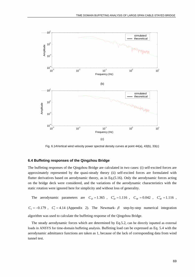
TIME DOMAIN BUFFETING ANALYSIS OF LARGE-SPAN CABLE-STAYED BRIDGE
69
10-3 10-2 10-1 100 10110-4
10-2
100
102
Frequency (Hz)
Ampl
itude
(b)
10-3 10-2 10-1 100 10110-4
10-2
100
102
Frequency (Hz)
Ampl
itude
(c)
Fig. 6.14Vertical wind velocity power spectral density curves at point 44(a), 43(b), 33(c)
6.4 Buffeting responses of the Qingzhou Bridge
The buffeting responses of the Qingzhou Bridge are calculated in two cases: (i) self-excited forces are approximately represented by the quasi-steady theory (ii) self-excited forces are formulated with flutter derivatives based on aerodynamic theory, as in Eq.(5.16). Only the aerodynamic forces acting on the bridge deck were considered, and the variations of the aerodynamic characteristics with the static rotation were ignored here for simplicity and without loss of generality.
The aerodynamic parameters are 365.1=DC , 116.1=′DC , 042.0=MC , 116.1=′MC ,
179.0−=lC , 14.4=′lC (Appendix 2). The Newmark- β step-by-step numerical integration
algorithm was used to calculate the buffeting response of the Qingzhou Bridge.
The steady aerodynamic forces which are determined by Eq.5.2, can be directly inputted as external loads in ANSYS for time-domain buffeting analysis. Buffeting load can be expressed as Eq. 5.4 with the aerodynamic admittance functions are taken as 1, because of the lack of corresponding data from wind tunnel test.
simulatedtheoretical
simulatedtheoretical
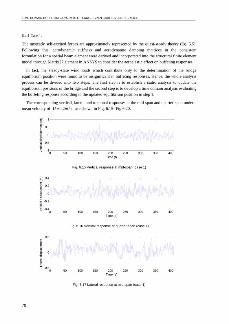
TIME DOMAIN BUFFETING ANALYSIS OF LARGE-SPAN CABLE-STAYED BRIDGE
70
6.4.1 Case 1,
The unsteady self-excited forces are approximately represented by the quasi-steady theory (Eq. 5.5). Following this, aerodynamic stiffness and aerodynamic damping matrices in the consistent formulation for a spatial beam element were derived and incorporated into the structural finite element model through Matrix27 element in ANSYS to consider the aeroelastic effect on buffeting responses.
In fact, the steady-state wind loads which contribute only to the determination of the bridge equilibrium position were found to be insignificant in buffeting responses. Hence, the whole analysis process can be divided into two steps. The first step is to establish a static analysis to update the equilibrium positions of the bridge and the second step is to develop a time domain analysis evaluating the buffeting response according to the updated equilibrium position in step 1.
The corresponding vertical, lateral and torsional responses at the mid-span and quarter-span under a mean velocity of smU /42= are shown in Fig. 6.15- Fig.6.20.
0 50 100 150 200 250 300 350 400-1
-0.5
0
0.5
1
Time (t)
Verti
cal d
ispl
acem
ent (
m)
Fig. 6.15 Vertical response at mid-span (case 1)
0 50 100 150 200 250 300 350 400-0.4
-0.2
0
0.2
0.4
Time (s)
Ver
tical
dis
plac
emen
t (m
)
Fig. 6.16 Vertical response at quarter-span (case 1)
0 50 100 150 200 250 300 350 400-0.5
0
0.5
Time (s)
Late
ral d
ispl
acem
ent
Fig. 6.17 Lateral response at mid-span (case 1)
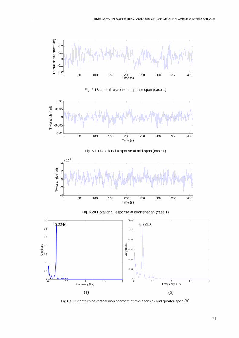
TIME DOMAIN BUFFETING ANALYSIS OF LARGE-SPAN CABLE-STAYED BRIDGE
71
0 50 100 150 200 250 300 350 400-0.2
-0.1
0
0.1
0.2
Time (s)
Late
ral d
ispl
acem
ent (
m)
Fig. 6.18 Lateral response at quarter-span (case 1)
0 50 100 150 200 250 300 350 400-0.01
-0.005
0
0.005
0.01
Time (s)
Twis
t ang
le (r
ad)
Fig. 6.19 Rotational response at mid-span (case 1)
0 50 100 150 200 250 300 350 400-4
-2
0
2
4x 10⁻³
Time (s)
Twis
t ang
le (r
ad)
Fig. 6.20 Rotational response at quarter-span (case 1)
0 0.5 1 1.5 20
0.1
0.2
0.3
0.4
0.5
0.6
0.7
Frequency (Hz)
Am
plitu
de
0 0.5 1 1.5 20
0.02
0.04
0.06
0.08
0.1
0.12
Frequency (Hz)
Am
plitu
de
(a) (b)
Fig.6.21 Spectrum of vertical displacement at mid-span (a) and quarter-span (b)
0.2246 0.2213
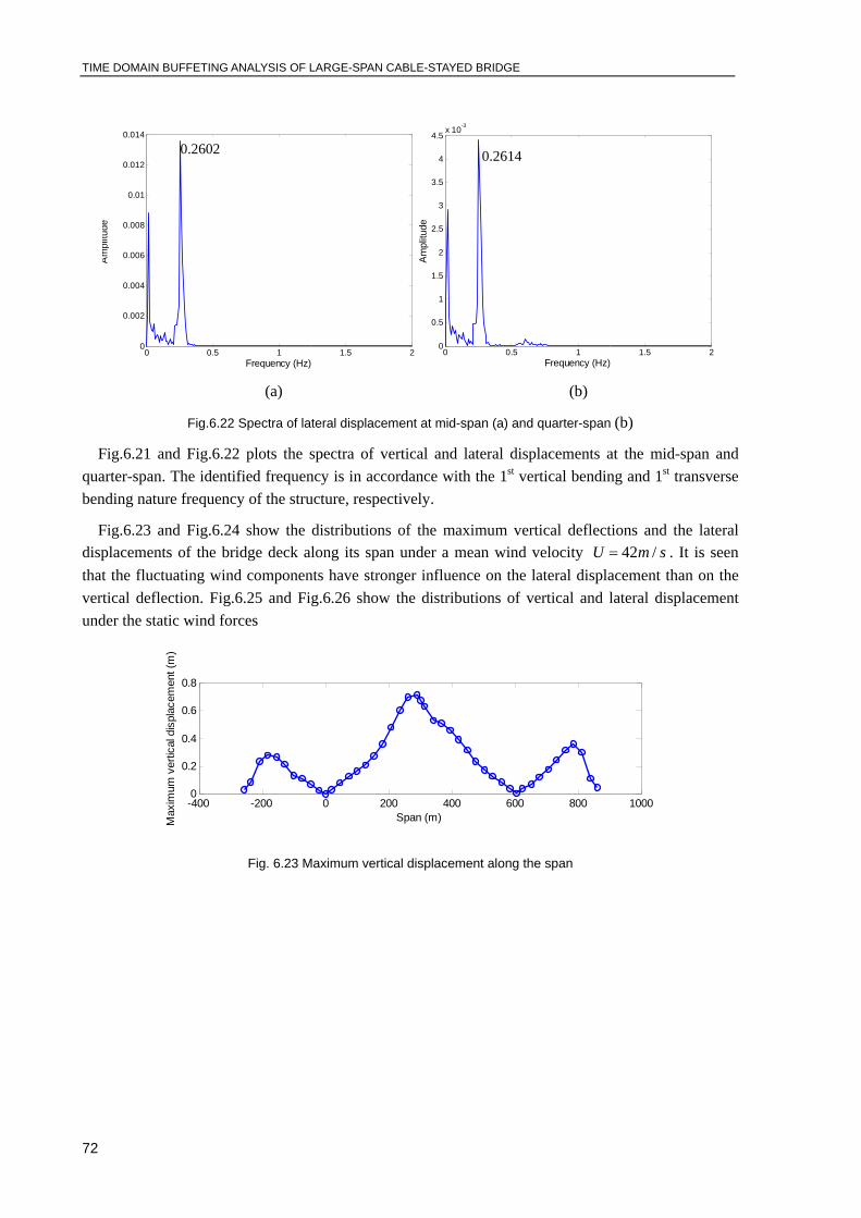
TIME DOMAIN BUFFETING ANALYSIS OF LARGE-SPAN CABLE-STAYED BRIDGE
72
0 0.5 1 1.5 20
0.002
0.004
0.006
0.008
0.01
0.012
0.014
Frequency (Hz)
Am
plitu
de
0 0.5 1 1.5 20
0.5
1
1.5
2
2.5
3
3.5
4
4.5x 10⁻³
Frequency (Hz)
Am
plitu
de
(a) (b)
Fig.6.22 Spectra of lateral displacement at mid-span (a) and quarter-span (b)
Fig.6.21 and Fig.6.22 plots the spectra of vertical and lateral displacements at the mid-span and quarter-span. The identified frequency is in accordance with the 1st vertical bending and 1st transverse bending nature frequency of the structure, respectively.
Fig.6.23 and Fig.6.24 show the distributions of the maximum vertical deflections and the lateral displacements of the bridge deck along its span under a mean wind velocity smU /42= . It is seen that the fluctuating wind components have stronger influence on the lateral displacement than on the vertical deflection. Fig.6.25 and Fig.6.26 show the distributions of vertical and lateral displacement under the static wind forces
-400 -200 0 200 400 600 800 10000
0.2
0.4
0.6
0.8
Span (m)Max
imum
ver
tical
dis
plac
emen
t (m
)
Fig. 6.23 Maximum vertical displacement along the span
0.2602 0.2614
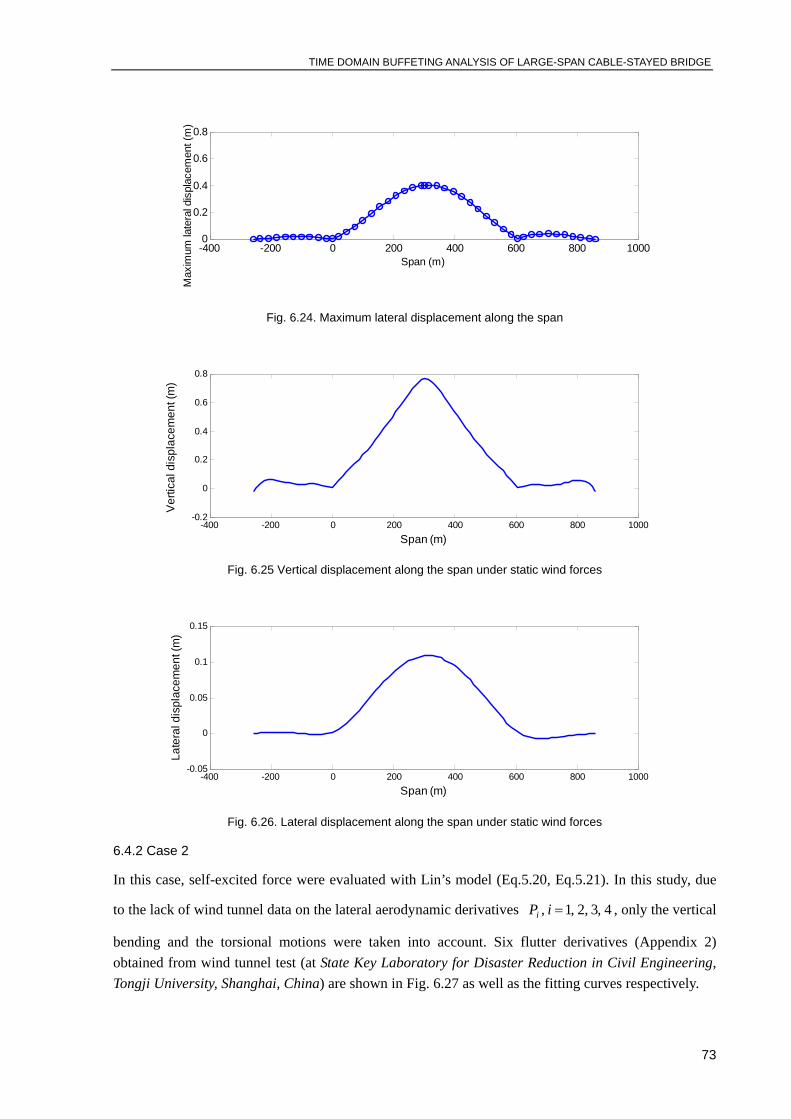
TIME DOMAIN BUFFETING ANALYSIS OF LARGE-SPAN CABLE-STAYED BRIDGE
73
-400 -200 0 200 400 600 800 10000
0.2
0.4
0.6
0.8
Span (m)
Max
imum
late
ral d
ispl
acem
ent (
m)
Fig. 6.24. Maximum lateral displacement along the span
-400 -200 0 200 400 600 800 1000-0.2
0
0.2
0.4
0.6
0.8
Span (m)
Ver
tical
dis
plac
emen
t (m
)
Fig. 6.25 Vertical displacement along the span under static wind forces
-400 -200 0 200 400 600 800 1000-0.05
0
0.05
0.1
0.15
Span (m)
Late
ral d
ispl
acem
ent (
m)
Fig. 6.26. Lateral displacement along the span under static wind forces
6.4.2 Case 2
In this case, self-excited force were evaluated with Lin’s model (Eq.5.20, Eq.5.21). In this study, due
to the lack of wind tunnel data on the lateral aerodynamic derivatives 4,3,2,1, =iPi , only the vertical
bending and the torsional motions were taken into account. Six flutter derivatives (Appendix 2) obtained from wind tunnel test (at State Key Laboratory for Disaster Reduction in Civil Engineering, Tongji University, Shanghai, China) are shown in Fig. 6.27 as well as the fitting curves respectively.
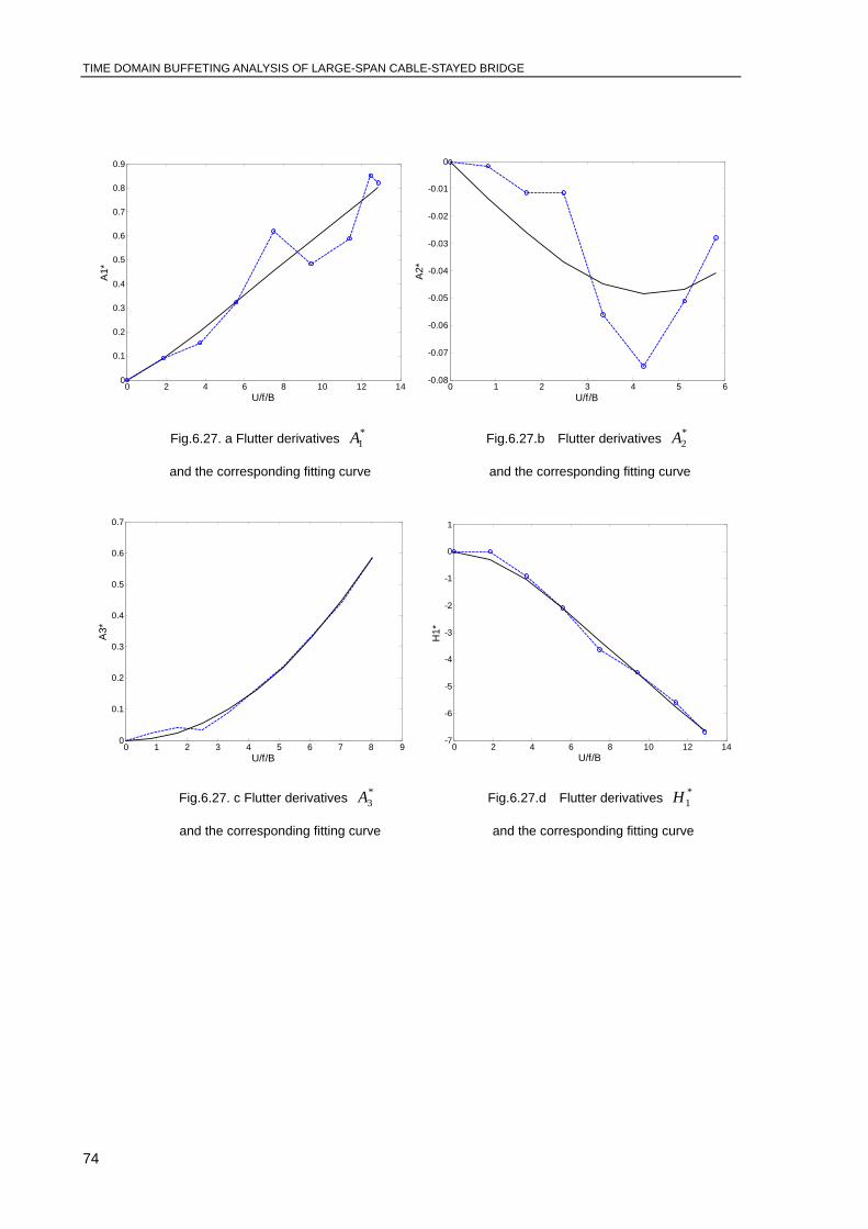
TIME DOMAIN BUFFETING ANALYSIS OF LARGE-SPAN CABLE-STAYED BRIDGE
74
0 2 4 6 8 10 12 140
0.1
0.2
0.3
0.4
0.5
0.6
0.7
0.8
0.9
U/f/B
A1*
0 1 2 3 4 5 6-0.08
-0.07
-0.06
-0.05
-0.04
-0.03
-0.02
-0.01
0
U/f/B
A2*
Fig.6.27. a Flutter derivatives *1A Fig.6.27.b Flutter derivatives *
2A
and the corresponding fitting curve and the corresponding fitting curve
0 1 2 3 4 5 6 7 8 90
0.1
0.2
0.3
0.4
0.5
0.6
0.7
U/f/B
A3*
0 2 4 6 8 10 12 14
-7
-6
-5
-4
-3
-2
-1
0
1
U/f/B
H1*
Fig.6.27. c Flutter derivatives *3A Fig.6.27.d Flutter derivatives *
1H
and the corresponding fitting curve and the corresponding fitting curve
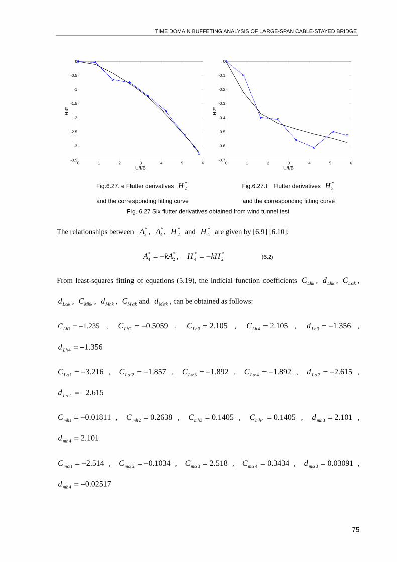
TIME DOMAIN BUFFETING ANALYSIS OF LARGE-SPAN CABLE-STAYED BRIDGE
75
0 1 2 3 4 5 6-3.5
-3
-2.5
-2
-1.5
-1
-0.5
0
U/f/B
H3*
0 1 2 3 4 5 6
-0.7
-0.6
-0.5
-0.4
-0.3
-0.2
-0.1
0
U/f/B
H2*
Fig.6.27. e Flutter derivatives *2H Fig.6.27.f Flutter derivatives *
3H
and the corresponding fitting curve and the corresponding fitting curve
Fig. 6.27 Six flutter derivatives obtained from wind tunnel test
The relationships between *2A , *
4A , *2H and *
4H are given by [6.9] [6.10]:
*2
*4 kAA −= , *
2*4 kHH −= (6.2)
From least-squares fitting of equations (5.19), the indicial function coefficients LhkC , Lhkd , kLC α ,
kLd α , MhkC , Mhkd , kMC α and kMd α , can be obtained as follows:
235.11 −=LhC , 5059.02 −=LhC , 105.23 =LhC , 105.24 =LhC , 356.13 −=Lhd ,
356.14 −=Lhd
216.31 −=αLC , 857.12 −=αLC , 892.13 −=αLC , 892.14 −=αLC , 615.23 −=αLd ,
615.24 −=αLd
01811.01 −=mhC , 2638.02 =mhC , 1405.03 =mhC , 1405.04 =mhC , 101.23 =mhd ,
101.24 =mhd
514.21 −=αmC , 1034.02 −=αmC , 518.23 =αmC , 3434.04 =αmC , 03091.03 =αmd ,
02517.04 −=mhd

TIME DOMAIN BUFFETING ANALYSIS OF LARGE-SPAN CABLE-STAYED BRIDGE
76
The dynamic displacement responses of the bridge at mid span and quarter span under a mean wind velocity smU /42= are shown in Fig6.28-6.33.
0 50 100 150 200 250 300 350 400-1
-0.5
0
0.5
1
Fig. 6.28 Vertical response at mid-span (case 2)
0 50 100 150 200 250 300 350 400-0.2
0
0.2
0.4
Fig. 6.29 Vertical response at quarter-span (case 2)
0 50 100 150 200 250 300 350 400-0.5
0
0.5
eca
spac
ee
(
Fig. 6.30 Lateral response at mid-span (case 2)
Verti
cal D
ispl
acem
ent (
m)
Time (s)
Verti
cal D
ispl
acem
ent (
m)
Time (s)
Late
ral D
ispl
acem
ent (
m)
Time (s)
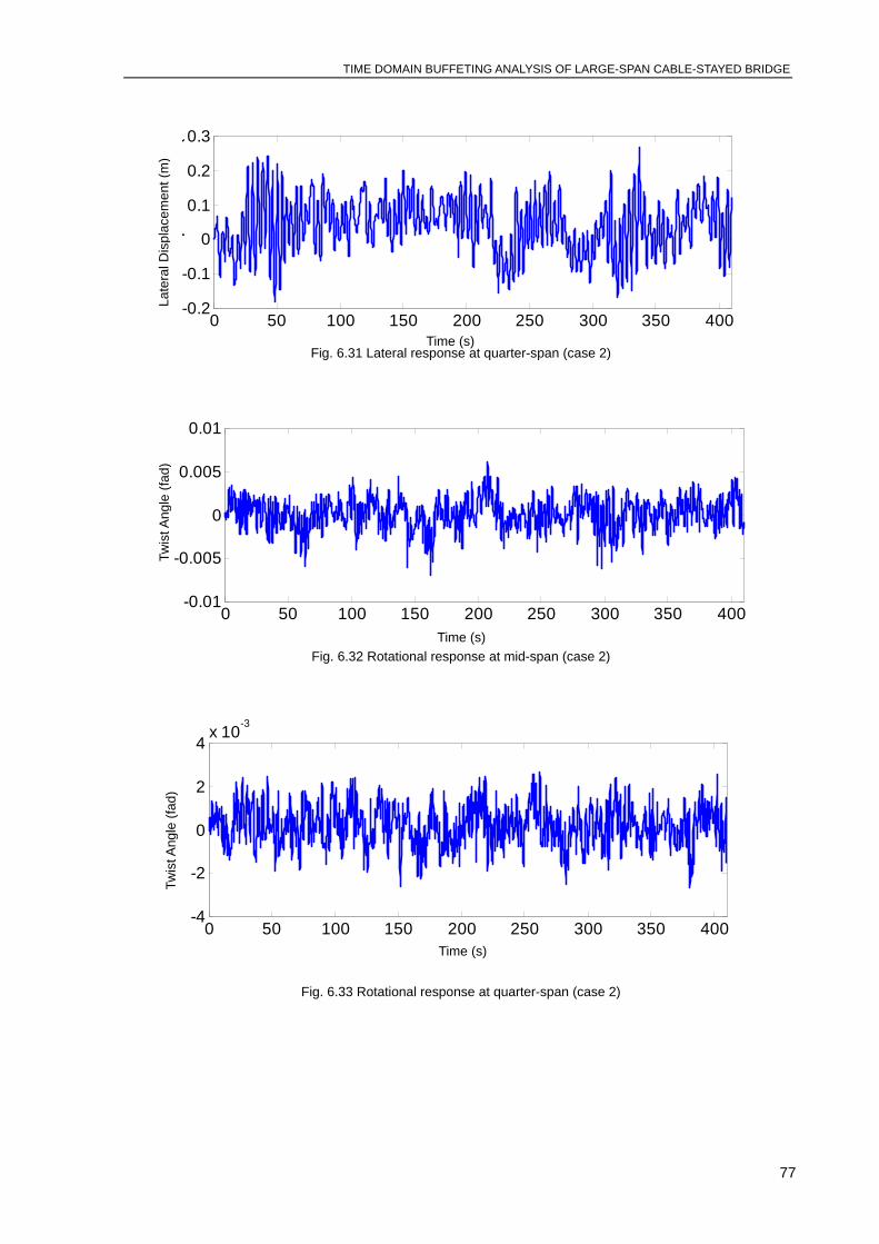
TIME DOMAIN BUFFETING ANALYSIS OF LARGE-SPAN CABLE-STAYED BRIDGE
77
0 50 100 150 200 250 300 350 400-0.2
-0.1
0
0.1
0.2
0.3
p(
Fig. 6.31 Lateral response at quarter-span (case 2)
0 50 100 150 200 250 300 350 400-0.01
-0.005
0
0.005
0.01
Fig. 6.32 Rotational response at mid-span (case 2)
0 50 100 150 200 250 300 350 400-4
-2
0
2
4x 10⁻³
Fig. 6.33 Rotational response at quarter-span (case 2)
Late
ral D
ispl
acem
ent (
m)
Time (s)
Twis
t Ang
le (f
ad)
Time (s)
Time (s)
Twis
t Ang
le (f
ad)

TIME DOMAIN BUFFETING ANALYSIS OF LARGE-SPAN CABLE-STAYED BRIDGE
78
20 22 24 26 28 30 32 34 36 380.1
0.11
0.12
0.13
0.14
0.15
0.16
0.17
0.18
0.19
0.2
Fig.6.34 Variation of RMS of vertical displacement at mid span
Fig.6.34 shows the RMS of vertical displacement responses at mid span obtained in case 1 and case 2 comparing with the result without considering self-excited forces, at mean wind velocities
smU /36,32,28,24= . It is shown that the results obtained with considering self-excited forces are smaller than those obtained without considering self-excited forces. The reason is that the aeroelastic damping has often a mitigating effect caused by positive aerodynamic damping at lower wind velocities, and the mitigating effects of aerodynamic damping. The results obtained in case 2 are about 7% smaller than in case 1.
Verti
cal D
ispl
acem
ent (
m)
U (m/s)
Case2
Without self-excited forces
26 28 30 32 34 36 38 40 42 44

TIME DOMAIN BUFFETING ANALYSIS OF LARGE-SPAN CABLED-STAYED BRIDGE
79
7 CONCLUSIONS
This thesis centered on the time domain buffeting analysis of large-span cable stayed bridge. Five issues were pursued: (i) understanding of wind induced buffeting theory; (ii) simulation of wind speed time series; (iii) time domain buffeting analysis based on quasi-steady hypotheses (iv) time domain buffeting analysis based on aeroelastic hypotheses (v) comparison the results of different method.
In the first three chapters, firstly the development history and research method of bridge wind engineering are introduced to get a general idea of wind engineering. Then the characteristics of cable-stayed bridge, the characteristics of wind field and wind induced vibration of bridges are studied to prepare for the large-span cable-stayed bridge buffeting analysis in the following steps.
In Chapter 4, autoregressive (AR) model is used to simulate the wind velocity of three dimensional fields in accordance with the time and space dependent characteristics of the 3-D fields. Based on the built MATLAB programming, this chapter discusses in detail the issues of the AR model induced by matrix form in the simulation and proposes the corresponding solving methods: the overrelaxation iteration to solve the large sparse matrix equation produced by large number of degrees of freedom of structures; the improved Gauss formula to calculate the numerical integral equations which integral function contain oscillating functions. This chapter also follows the method of ascertaining the rank of the AR model. At the end of this chapter, a four-node numerical model is presented, The results of the comparison among power spectral densities are found to be in a very close agreement. The correlation functions reveal the spatial and time correlation characteristics of the wind velocity well.
Chapter 5, introduced the method of time domain buffeting analysis as well as the related concepts, and the specific implementation method in ANSYS. Under quasi-steady hypotheses, the buffeting forces simulated based on the span-wise coherence of buffeting forces and also considering the aerodynamic admittance functions, together with the steady aerodynamic forces are applied as external loads to the structural model to analyze the buffeting responses in time domain. In order to account for self-excited forces, elemental aeroelastic stiffness and aeroelastic damping matrices for spatial beam elements are derived following the quasi-steady theory and are incorporated in buffeting analysis through the user-defined Matrix27 element in ANSYS. In aeroelastic hypotheses, to take into account unsteady fluid memory effects, self-excited force is expressed in terms of convolution integrals
TIME DOMAIN BUFFETING ANALYSIS OF LARGE-SPAN CABLE-STAYED BRIDGE
80
between bridge deck motion and impulse response functions, with flutter derivatives identified from wind tunnel test. The frequency-related flutter derivatives are transformed into indicial functions, using Lin’s approach. An iterative process is presented for the nonlinearity of self-excited force, and implemented by developing the program in APDL language based on ANSYS system. .
In Chapter 6, a numerical model of Qingzhou Bridge, China, was introduced. Then The wind time velocity series on the bridge deck was generated to be composed of 87 wind velocity waves at 87 different points distributed along the deck of the bridge, using AR model. After that both of these two approaches are applied on Qingzhou Bridge. It is showed that the analysis results by two methods are basically consistent with each other. And the approach based on quasi-steady theory get a result bigger than that of the other approach.
TIME DOMAIN BUFFETING ANALYSIS OF LARGE-SPAN CABLE-STAYED BRIDGE
81
REFERENCES
[1.1] Davenport, A.G. (1962). Buffeting of a Suspension Bridge by Storm Winds, J. of Struct. Div., ASCE, vol. 88, No.3, pp. 233-268.
[1.2] Scanlan, R.H. and Gade, R.H. (1977). Motion of Suspended Bridge Spans under Gusty Wind, J Struct. Div, ASCE, v103 n9, pp. 1867-1883
[1.3] Scanlan, R. H. (2000). Bridge Deck Aeroelastic Admittance Revisited, ASCE, J. Bridge Engng., 5(1), pp. 1-7.
[1.4] Lin, Y.K., Li.Q.C., and Su, T.C. (1993). Application of a New Wind Turbulence Model in Predicting Motion Stability of Wind-Excited Long-Span Bridges, Journal of Wind Engineering and Industrial Aerodynamics v 49 n 1-3, pt 1, pp. 507-516.
[2.1] I. van der Hoven, Power spectrum of horizontal wind speed in the frequency range from 0.0007 to 900 cycles/hour, J. Meteorol. 14 (1957), pp. 160–164.
[2.2] A.G. Davenport, The application of statistical concepts to the wind loading of structures, Proc. ICE 19 (1961), pp. 449–471.
[2.3] Murakami, S., Mochida, A., 1999. Past, present and future of CWE. The view from 1999. In: Proceedings of the 10th International Conference on Wind Engineering, Copenhagen, pp. 91–104.
[2.4] Wind and Structures, 2005. In: Holmes, J. (Ed.), Special Edition on the IAWE Codification Initiative
[2.5] Kareem, A., 2003. A tribute to Jack E Cermak—wind effects on structures: a reflection on the past and outlook for the future. In: Proceedings of the 11th International Conference on Wind Engineering, Lubbock, pp. 1–28.
[2.6] Theodorsen, T., 1935. General theory of aerodynamic instability and the mechanism of flutter. NACA Report No. 496, US. National Advisory Committee for Aeronautics, Langley, VA.
[2.7] R.H. Scanlan and W.H. Lin, Effects on turbulence on bridge flutter derivatives, J. Eng. Mech., ASCE 104 (EM4) (1978), pp. 719–733. View Record in Scopus | Cited By in Scopus (13)
[2.8] R.H. Scanlan, The action of flexible bridges under wind, II: Buffeting theory, Journal of Sound and Vibration, Volume 60, Issue 2, 22 September 1978, Pages 201-211
[2.9] R.H. Scanlan and R.H. Gade, Motion of suspension bridge spans under gusty wind, ASCE Journal of the Structural Division 103 (1977) (ST9), pp. 1867–1883. View Record in Scopus | Cited By in Scopus (31)
[2.10] John D. Holmes, Wind loading of structures, 2007
[2.11] K. Billah and R. Scanlan, Resonance, Tacoma Narrows Bridge Failure, and Undergraduate Physics Textbooks, American Journal of Physics, 59(2), 118—124,1991
[2.12] Maureen Byko . Materials Give Roller Coaster Enthusiasts a Reason to Scream. The Minerals, Metals & Materials Society. Retrieved 2009-02-22.
TIME DOMAIN BUFFETING ANALYSIS OF LARGE-SPAN CABLE-STAYED BRIDGE
82
[2.13] Steinman, D.B. and Watson, S.R., 1957. Bridges and their Builders, Dover, New York.
[2.14] Billington, DP, 1977, History and esthetics in suspension bridges, ASCE Journal of the Structural Division 103: 1655-72.
[2.15] Baker, B. 1884, The Forth Bridge, Engineering 38:213.
[2.16] Kernot, WC 1983, Wind pressure, Proceding, Australasian Society for the Advancement of Science V:573-81.
[3.1] Emil Simiu, Robert H.Scanlan, Wind Effects on Structures, 1985, 31-77
[3.2] Eurocode 1 Actions on structures Part1-4: Wind actions (EN1991-1-4.6)
[3.3] American Minimum Design Loads for Buildings and Other Structures (ASNI/ASCE7-95)
[3.4] Chinese load code for the design of building structures (GB5009-2002)
[3.5] J.L.Lumley and H.A.Panofsky, The Structure of Atmospheric Turbulence, Wiley, New York, 1964
[3.6] L. Kristensen and N. O. Jensen, Lateral Coherence in Isotropic Turbulence and in the Natural Wind, Bound Layer Meterol., 17(1979), 353-373.
[3.7] J.D. Riera and A. G.. Davenport, Wind Effects on Buildings and Structures, pp. 177-179.
[3.8] John D.Hollmes, Wind loading of structures, pp.57-58
[4.1] Samaras, E., Shinozuka, M. and Tsurui, A. 1985 Journal of Engineering Mechanics, ASCE, 111(3), 449-461, ARMA representation of random vector processes.
[4.2] Li, Y. and Kareem, A. 1990, Journal of Wind Engineering and Industrial Aerodynamics, 36,415-427, ARMA representation of wind field.
[4.3] Kamal, L, and Jafri, Y. Z. 1997, Solar Energy, 61(1), 23-32, Time series models to simulate and forecast hourly averaged wind speed in Quetta, Pakistan.
[4.4] Kho, S., Baker, C. and Hoxey, R. 2002, Journal of Wind Engineering and Industrial Aerodynamics, 90,1831-1842, POD/ARMA reconstruction of the surface pressure field around a low rise structure.
[4.5] Kizilkaya, A. and Kayran, A. H. 2006, Digital signal processing, 16, 670-681, ARMA model parameter estimation based on the equivalent MA approach.
[4.6] Iwatani, Y. 1982, Journal of Wind Engineering,11,5-14, Simulation of multidimensional wind fluctuations having any arbitrary power spectra and cross spectra.
[4.7] Iannuzzi, A. and Spinelli, P. 1987, Journal of Structural Engineering, ASCE, 113(10), 2382-2398, Artificial wind generation and structural response.
[4.8] Huang, Z. and Chalabi, Z. S. 1995, Journal of Wind Engineering and Industrial Aerodynamics, 56, 311-322, Use of time-series analysis to model and forecast wind speed.

TIME DOMAIN BUFFETING ANALYSIS OF LARGE-SPAN CABLE-STAYED BRIDGE
83
[4.9] Statopoulos, T., Kumat, K. S. and Mohammadian, A.R. 1996, Journal of Wind EngineJournal of Wind Engineering and Industrial Aerodynamicsering and Industrial Aerodynamics, 65, 143-153, Design wind pressure coefficients for monoslope roofs: A time series approach.
[4.10] Facchinim L. 1996, Journal of Wind Engineering and Industrial Aerodynamics, 64, 187-202, the numerical simulation of Gaussian cross-correlated wind velocity fluctuations by means of a hybrid model.
[4.11] Li, Y-Q and Dong, S-L. 2001, Spatial Structure, 7(3), 3-11, Random wind load simulation and computer program for large-span spatial structures. (in Chinese)
[4.12] Poggim P., Muselli, M., Notton, G., Cristofarim C. and Louche, A. 2003, Energy Conversion and Management, 44, 3177-3196, Forecasting and simulating wind speed in Corsica by using an autoregressive model.
[4.13] Roy, A. and Fuller, W. A. 2001, J. Bus Econ Stat., 19, 482-493, Estimation for autoregressive time series with a roof near one.
[4.14] Kim, J. H. 2003, International Journal of Forecasting, 19, 493-502, Forecasting autoregressive time series with bias-corrected parameter estimators.
[4.15] Strube,H.W. 1985, Signal Process, 8(1), 53-74, A generalization of correlation functions and the Wiener-Khinchin theorem.
[4.16] Panofsky, H. A. 1974, Annual Review of Fluid Mechanics, 6,147-177, the atmospheric boundary layer below 150 meters.
[4.17] Schlindwein, F. S. and Evans, D. H. 1990, Ultrasound Med. Biol. 16(1), 81-91, selection of the order of autoregressive models for spectral analysis of Doppler Ultrasound signals.
[4.18] Akaike, H. 1974, IEEE Trans. Automatic Control, 19, 716-723, A new look at the statistical model identification.
[4.19] Pappas, S. S., Leros, A. K., and Katsikas S. K. 2006, Digital Signal Processing, 16, 782-795, Joint order and parameter estimation of multivariate autoregressive models using multi-model partitioning theory.
[4.20] Martinsm M. M., Trigo, M. E. And Santos. M. M. 1996, Linear Algebra. Appl., 232, 131-147, An error bound for the SSOR and USSOR methods.
[4.21] Gander, W. and Gautschi, W. 2000, Numerical Mathematics, 40, 84,101, Adaptive quadrature revisited.
[4.22] Wang, A-H. 1994, Journal of Building Structure, 15(1), 44-52, Simulation of wind loading. (in Chinese)
[4.23] Weicheng Gao and Yanlei Yu, Journal of Wind and Structure, vol. 11, No.3 (2008), pp. 241-256, Wind velocity simulation of spatial three-dimensional fields based on autoregressive model.
[5.1] T.J.A..AGRA, 1988, Computer & Structures 30, 593-600. The analysis of aerodynamic flutter of suspension bridges.

TIME DOMAIN BUFFETING ANALYSIS OF LARGE-SPAN CABLE-STAYED BRIDGE
84
[5.2] R.H SCANLAN, Aeroelastic simulation of bridges, 1983, Journal of Structural Engineering, ASCE 109, 2829-2837.
[5.3] A.G. Davenport, Buffeting of a suspension bridge by storm winds, J. Struct. Div. ASCE 88-3 (1962) 233–268.
[5.4] E. Simiu, R.H. Scanlan, Wind Effects on Structures, Wiley, USA, 1996.
[5.5] G.L. Larose, J. Mann, Gust loading on streamlined bridge decks, J. Fluids Struct. 12 (1998) 511–536.
[5.6] X.G. Hua, Z.Q. Chen, Y.Q. Ni and J.M. Ko, Flutter analysis of long-span bridges using ANSYS, Wind Struct 10 (1) (2007), pp. 61–82.
[5.7] Swanson Analysis Systems Inc. (SASI). ANSYS user’s manual, version 8.0. Houston (PA). 2004.
[5.8] R. H. SCANLAN, J. G. BELIVEAU and K. S. BUDLONG, Indicial aerodynamic functions for bridge decks. Journal of Engineering Mechanics, ASCE 100 (1974), pp. 657–672.
[5.9] C. G. BUCHER and Y. K. LIN, Stochastic stability of bridges considering coupled modes. Journal of Engineering Mechanics, ASCE 114 (1988), pp. 2055–2071.
[5.10] T. Theodorsen, General theory of aerodynamic instability and the mechanism of flutter, NACA Report 496, US Nat. Advisory Committee for Aeronautics, Langley, VA 1935.
[5.11] R.H. Scanlan, J.J. Tomko, Airfoil and bridge deck flutter derivatives, J. Eng. Mech. Div. ASCE 97 (EM6) (1971) 1717–1737.
[5.12] R.H. Scanlan, On flutter and buffeting mechanisms in long-span bridges, Prob. Eng. Mech. 3 (1) (1988) 22–27.
[5.13] LI Yong-le, LIAO Hhai-li, QIANG Shi-zhong, Nonlinear Time Domain Bufeting Response Analysis for Long-Span Railway Cable-Stayed Bridge, Journal of Southwest Jiaotong University, 39(3) 2004 (Chinese)
[5.14]Scanlan, R. H. (1978). ‘‘The action of flexible bridges under wind. 2: Buffeting theory.’’ J. Sound and Vibration, 60(2), 201–211.
[5.15] Chen, X., Matsumoto, M., and Kareem, A. (2000). ‘‘Aerodynamic coupling effects on the flutter and buffeting of bridges.’’ J. Engrg. Mech., ASCE, 126(1), 17–26.
[5.16]Jain, A., Jones, N. P., and Scanlan, R. H. (1996). ‘‘Coupled flutter and buffeting analysis of long-span bridges.’’ J. Struct. Engrg., ASCE, 122(7), 716–725.
[5.17]Katsuchi, H., Jones, N. P., and Scanlan, R. H. (1999). ‘‘Multimode coupled flutter and buffeting analysis of the Akashi-Kaikyo Bridge.’’ J.Struct. Engrg., ASCE, 125(1), 60–70.
[5.18]Lin, Y.K., and Yang, J.N.(1983), Multimode Bridge Response to Wind Excitations, Journal of Engineering Mechanics, 109(2), pp. 586-603.
[5.19] Scanlan, R.H. (1984), Role of Indicial Functions in Buffeting Analysis of Bridges, Journal of Structural Engineering, ASCE, 110(7), pp. 1433-1446.
[5.20] Chen X, Matsumoto M, Kareem A. (2000), Time Domain Flutter and Buffeting Response
TIME DOMAIN BUFFETING ANALYSIS OF LARGE-SPAN CABLE-STAYED BRIDGE
85
Analysis of Bridges. Journal of Engineering Mechanics, ASCE, 126, 7-16.
[5.21] Z.Q. Chen, Y. Han, X.G. Hu, Y.Z. Luo, Investigation On Influence Factors Of Buffeting Response Of Bridges And Its Aeroelastic Model Verification For Xiaoguan Bridge. Journal of Engineering Structures, 31(2009), pp. 417-431.
[5.22] Alexandre de la Foye,Calcul de la reponse dynamique des structures elancees a la turbulence du vent,Thèse de doctorat,le 9 juillet 2001,Universite de Nantes ecole Doctorale
[5.23] Q. Ding, P. K. K. Lee and S. H. Lo, Time domain buffeting analysis of suspension bridges subjected to turbulent wind with effective attack angle, Journal of sound and vibration (2000) 233(2),311-327
[6.1] Wei-Xin Ren, Xue-Lin Peng, 2005, Computer & Structures 83, 536-550. Baseline finite element modeling of a large span cable-stayed bridge through field ambient vibration tests.
[6.2] Wei-Xin Ren, You-Qin Lin and Xue-Lin Peng, 2007, J. Bridge Engineering ASCE, Volume 12, Issue 2, pp. 261-270, Field Load Tests and Numerical Analysis of Qingzhou Cable-Stayed Bridge.
[6.3] Wilson JC, Gravelle W. Modeling of a cable-stayed bridge for dynamic analysis. Earthquake Engrg Struct Dyn. 1991;20:707–22.
[6.4] Zhu LD, Xiang HF, Xu YL. Triple-girder model for modal analysis of cable-stayed bridges with warping effect. Engrg Struct 2000;22(10):1313–23.
[6.5] Ren WX, Obata M. Elastic–plastic seismic behavior of long span cable-stayed bridges. J Bridge Engrg ASCE 1999;4(3):194–203.
[6.6] Ansys help document
[6.7] Nazmy AS, Abdel-Ghaffar AM. Nonlinear earthquakeresponse analysis of long-span Cable-stayed bridges: theory. Earthquake Engrg Struct Dyn 1990;19(1):45–62.
[6.8] Nazmy AS, Abdel-Ghaffar AM. Nonlinear earthquakeresponse analysis of long-span cable-stayed bridges: applications. Earthquake Engrg Struct Dyn 1990;19(1):63–76.
[6.9] R.H. Scanlan, N.P. Jones and L. Singh, Inter-relations among flutter derivatives, J. Wind Eng. Ind. Aerodyn. 69–71 (1997), pp. 829–837.
[6.10] F.Tubino, Relationships among aerodynamic admittance functions, flutter derivatives and static coefficients for long span bridges. Journal of Wind Engineering and Industrial Aerodynamics, Volume 93, Issue 21, December, pp. 929-950

TIME DOMAIN BUFFETING ANALYSIS OF LARGE-SPAN CABLE-STAYED BRIDGE
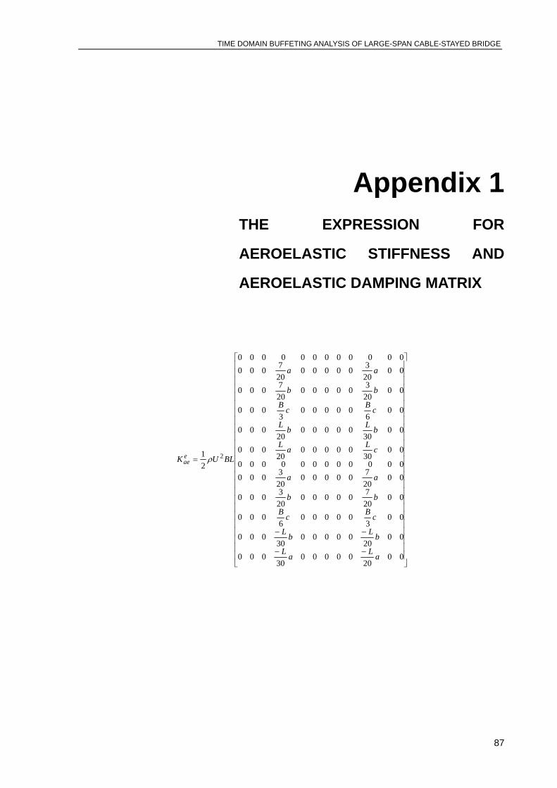
TIME DOMAIN BUFFETING ANALYSIS OF LARGE-SPAN CABLE-STAYED BRIDGE
87
Appendix 1 THE EXPRESSION FOR
AEROELASTIC STIFFNESS AND
AEROELASTIC DAMPING MATRIX
⎥⎥⎥⎥⎥⎥⎥⎥⎥⎥⎥⎥⎥⎥⎥⎥⎥⎥⎥⎥⎥⎥⎥⎥⎥
⎦
⎤
⎢⎢⎢⎢⎢⎢⎢⎢⎢⎢⎢⎢⎢⎢⎢⎢⎢⎢⎢⎢⎢⎢⎢⎢⎢
⎣
⎡
−−
−−
=
0020
0000030
000
0020
0000030
000
003
000006
000
0020700000
203000
0020700000
203000
000000000000
0030
0000020
000
0030
0000020
000
006
000003
000
0020300000
207000
0020300000
207000
000000000000
21 2
aLaL
bLbL
cBcB
bb
aa
cLaL
bLbL
cBcB
bb
aa
BLUK eae ρ
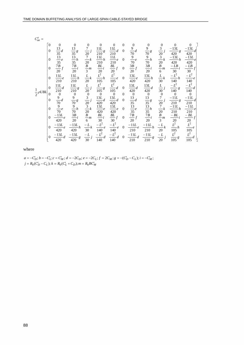
TIME DOMAIN BUFFETING ANALYSIS OF LARGE-SPAN CABLE-STAYED BRIDGE
88
⎥⎥⎥⎥⎥⎥⎥⎥⎥⎥⎥⎥⎥⎥⎥⎥⎥⎥⎥⎥⎥⎥⎥⎥⎥⎥⎥
⎦
⎤
⎢⎢⎢⎢⎢⎢⎢⎢⎢⎢⎢⎢⎢⎢⎢⎢⎢⎢⎢⎢⎢⎢⎢⎢⎢⎢⎢
⎣
⎡
−−−−−−−−
−−−−−−−−
−−−
−−
−−
−−
−−
−−
−−
−−
=
dLgLjLgLdLdLdLjLgLdL
eLhLkLhLeLeLeLkLhLeL
fBLiBLmBiBfBfBLiBLmBiBeL
eLhLkheeLeLkhe
dLgLjgddLdLjgd
dLgLjLdLdLdLgLjLgLdL
eLhLkLhLeLeLhLkLhLeL
fLBiLBmBiBfBfBLiBLmBiBfB
eLhLkheeLhLkhe
dLgLjgddLgLjgd
UBL
Ceae
1051052021011
210110
1401403042013
420130
1051052021011
210110
1401403042013
420130
20203207
2070
30306203
420130
21011
21011
207
3513
35130
42013
42013
203
709
7090
21011
21011
207
3513
35130
42013
42013
203
709
7090
00000000000014014030420
13420130
1051052021011
210110
1401403042013
420130
1051052021011
210110
30306203
2030
20203207
2070
42013
42013
203
709
7090
21011
21011
207
3513
35130
42013
42013
203
709
7090
21011
21011
207
3513
35130
000000000000
21
2222
2222
2222
2222
ρ
where
MDLLD
MLDMLDMLDCBRmCCRkCCRj
CiCCgCfCeCdCcCbCa′=+′=−′=
′−=−′−==−=−=′=′−=′−=
000 );();(;);(;2;2;2;;;

TIME DOMAIN BUFFETING ANALYSIS OF LARGE-SPAN CABLE-STAYED BRIDGE
89
Appendix 2 AERODYNAMIC COEFFICIENTS
FROM WIND TUNNEL TEST
Flutter derivative
a) Flutter derivatives with a attack angle o3
fBU / *1A fBU / *
2A fBU / *3A
0.00000 0.00000 0.00000 0.00000 0.00000 0.00000
1.87603 0.01318 0.82759 -0.00412 0.84401 0.00674
3.70443 0.0626 1.66174 -0.04119 1.69294 0.0309
5.54516 0.25206 2.50082 -0.03954 2.54926 0.06067
6.45484 0.21334 2.92939 -0.03954 2.97783 00.07022
7.38095 0.15568 3.36782 -0.03954 3.42282 0.11292
8.3119 0.37479 3.80378 -0.0313 3.87521 0.15787
8.75944 0.48847 4.4803 -0.00659 4.30952 0.17135
9.2578 0.35502 4.80542 0.27753
9.74138 0.46623 5.25287 0.27921

TIME DOMAIN BUFFETING ANALYSIS OF LARGE-SPAN CABLE-STAYED BRIDGE
90
fBU / *1H fBU / *
2H fBU / *3H
0.00000 0.00000 0.00000 0.000 0.00000 0.00000
1.87603 -0.06613 1.008 -0.085 0.82759 -0.02984
3.70443 -0.96613 2.024 -0.749 1.66174 -0.08306
5.54516 -2.34113 3.046 -0.609 2.50082 -0.30726
6.45484 -2.83387 3.568 -0.306 2.92939 -0.57742
7.38095 -3.67097 4.102 -0.204 3.36782 -0.80806
8.3119 -4.10645 4.633 -0.044 3.80378 -1.11452
8.75944 -4.24597 5.181 -0.084 4.02463 -1.1629
9.2578 -4.15645 5.457 0.070 4.25369 -1.36774
9.74138 -4.60806 4.4803 -1.60403
b) Flutter derivatives with a attack angle o0
fBU / *1A fBU / *
2A fBU / *3A
0.00000 0.00000 0.00000 0.00000 0.00000 0.00000
1.87274 0.09143 0.82841 -0.00165 0.83333 0.02303
3.72167 0.15404 1.66667 -0.01153 1.67077 0.04213
5.57718 0.32537 2.48358 -0.01153 2.50493 0.03539
7.50575 0.61944 3.34565 -0.05601 3.36535 0.09213
9.43021 0.4827 4.2266 -0.07496 4.24795 0.16292
11.40805 0.58814 5.13218 -0.05107 5.1486 0.23876
12.47619 0.85091 5.81363 -0.02801 6.07964 0.33764
12.87274 0.8196 7.04516 0.44213
8.03284 0.58596

TIME DOMAIN BUFFETING ANALYSIS OF LARGE-SPAN CABLE-STAYED BRIDGE
91
fBU / *1H fBU / *
2H fBU / *3H
0.00000 0.00000 0.0000 0.00000 0.00000 0.00000 1.87274 0.00887 0.82841 -0.09758 0.82841 -0.03548 3.72167 -0.90968 1.66667 -0.39839 1.66667 -0.6532 5.57718 -2.08871 2.48358 -0.41048 2.48358 -0.75484 7.50575 -3.63306 3.34565 -0.55726 3.34565 -1.23629 9.43021 -4.48548 4.2266 -0.6121 4.2266 -1.76452 11.40805 -5.59919 5.13218 -0.49839 5.13218 -2.60968 12.87274 -6.69758 5.81363 -0.523 5.59442 -3.02097
5.81363 -3.27339
c) Flutter derivatives with a attack angle o3−
fBU / *1A fBU / *
2A fBU / *3A
0.00000 0.00000 0.00000 0.00000 0.00000 0.00000
1.86946 0.08484 0.82841 0.00082 0.83498 0.132891
3.72906 0.1112 1.66502 0.014 1.6798 0.267348
5.6092 0.26606 2.49097 -0.00247 2.51487 0.400254
5.60509 0.34926 2.49179 -0.00247 3.37028 0.536397
7.57061 0.23641 3.33333 -0.04366 4.24384 0.675428
9.48522 0.39951 4.18883 -0.06343 5.13465 0.817205
11.40722 0.45881 5.07061 -0.06013 6.05501 0.963685
13.49097 0.60626 5.97783 -0.05107 6.54433 1.041562
15.60591 0.79077 7.35057 -0.04448 7.0353 1.119703
16.76026 0.63591 7.87767 -0.03295 7.49261 1.192486
17.87767 0.96211 8.0353 1.278858

TIME DOMAIN BUFFETING ANALYSIS OF LARGE-SPAN CABLE-STAYED BRIDGE
92
fBU / *1H fBU / *
2H fBU / *3H
0 0 0 0 0 0
1.86946 -0.05645 0.82841 -0.06855 0.82841 -0.03065
3.72906 -0.96855 1.66502 -0.17903 1.66502 0.01935
5.6092 -1.98306 2.49097 -0.39435 2.49097 -0.72903
5.60509 -1.91532 2.49179 -0.38226 2.49179 -0.73629
7.57061 -1.9871 3.33333 -0.84274 3.33333 -1.3629
9.48522 -2.60403 4.18883 -1.9919 4.18883 -1.79032
11.40722 -2.64919 5.07061 -1.62097 5.07061 -2.275
13.49097 -3.81935 5.97783 -1.8879 5.97783 -2.90242
15.60591 -3.77581 6.89409 -2.29274 6.89409 -3.64758
16.76026 -4.03871 7.35057 -2.48629 7.35057 -3.93548
17.87767 -4.94758 7.87767 -2.8 7.87767 -4.38629
Static coefficients evaluated at the angle of attack 0=β .
365.1=DC , 042.0=MC , 179.0−=lC ,
Derivatives of the static coefficients at the angle of attack 0=β .
116.1=′MC , 14.4=′lC
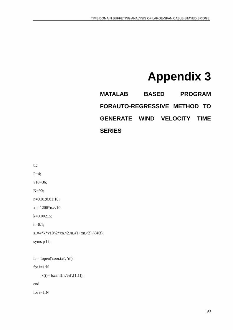
TIME DOMAIN BUFFETING ANALYSIS OF LARGE-SPAN CABLE-STAYED BRIDGE
93
Appendix 3 MATALAB BASED PROGRAM
FORAUTO-REGRESSIVE METHOD TO
GENERATE WIND VELOCITY TIME
SERIES
tic P=4;
v10=36;
N=90;
n=0.01:0.01:10;
xn=1200*n./v10;
k=0.00215;
ti=0.1;
s1=4*k*v10^2*xn.^2./n./(1+xn.^2).^(4/3);
syms p l f;
fr = fopen('coor.txt', 'rt');
for i=1:N
x(i)= fscanf(fr,'%f',[1,1]);
end
for i=1:N
TIME DOMAIN BUFFETING ANALYSIS OF LARGE-SPAN CABLE-STAYED BRIDGE
94
z(i)=fscanf(fr,'%f',[1,1]);
v(i)=(z(i)/10)^0.16*v10;
end
A=zeros(P*N);
for p=1:P
R=zeros(N);
for i=1:N
for j=i:N
H=inline('(4*k*v10^2*(1200*f/v10).^2)./f./(1+(1200*f/v10).^2).^(4/3).*(exp(-2*f*sqrt(8^2*dx.^2+10^2*dz.^2)/vt)).*cos(2*pi*f*(p-1)*ti)','f','k','dx','dz','ti','v10','vt','p');
vt=(v(i)+v(j));
dx=x(i)-x(j);
dz=z(i)-z(j);
R(i,j)=quadl(H,0.01,10,0.001,0,k,dx,dz,ti,v10,vt,p);
R(j,i)=R(i,j);
end
end
for l=1:P-p+1
A(((l-1)*N+1):(l*N),((l+p-1-1)*N+1):((l+p-1)*N))=R;
end
end
for i=1:P*N
for j=1:i
A(i,j)=A(j,i);
end
end

TIME DOMAIN BUFFETING ANALYSIS OF LARGE-SPAN CABLE-STAYED BRIDGE
95
R=zeros(N);
for i=1:N
for j=i:N
H=inline('(4*k*v10^2*(1200*f/v10).^2)./f./(1+(1200*f/v10).^2).^(4/3).*(exp(-2*f*sqrt(8^2*dx.^2+10^2*dz.^2)/vt)).*cos(2*pi*f*P*ti)','f','k','dx','dz','ti','v10','vt','P');
vt=(v(i)+v(j));
dx=x(i)-x(j);
dz=z(i)-z(j);
R(i,j)=quadl(H,0.01,10,0.001,0,k,dx,dz,ti,v10,vt,P);
R(j,i)=R(i,j);
end
end
B=A(1:N,(N+1):(N*P));
B=[B,R];
B=B';
X=A\B;
R0=A(1:N,1:N);
RN=R0;
for i=1:P
RN=RN-(X(((i-1)*N+1):(i*N),1:N))'*B(((i-1)*N+1):(i*N),1:N);
end
L=chol(RN);
L=L';
a=zeros(N,1024);
for i=1:N
a(i,:)=normrnd(0,1,1,1024);
end
V(1:N,1)=L*a(:,1);
for i=2:p
TIME DOMAIN BUFFETING ANALYSIS OF LARGE-SPAN CABLE-STAYED BRIDGE
96
V(1:N,i)=L*a(:,i);
for j=1:i-1
V(1:N,i)=(X(((j-1)*N+1):(j*N),:))'*V(1:N,(i-j))+V(1:N,i);
end
end
for i=(P+1):1024
V(1:N,i)=L*a(:,i);
for j=1:P
V(1:N,i)=(X(((j-1)*N+1):(j*N),:))'*V(1:N,(i-j))+V(1:N,i);
end
end
toc
V1=V(60,:);
t=(1:1024)*ti;
figure
subplot(2,1,1);
plot(t,V1,'b-');
xlabel('t(s)');
ylabel('v(t)');
[power,freq]=psd(V1,1024,10,boxcar(1024),0,'mean');
power=power*2/10;
subplot(2,1,2);
loglog(freq,power,'r-',n,s1,'g-');
maxlags=1024;
cx = xcorr(V1(1,:),V1(1,:),maxlags,'biased');
plot(cx)

TIME DOMAIN BUFFETING ANALYSIS OF LARGE-SPAN CABLE-STAYED BRIDGE
97
fid=fopen('windv.dat','a');
for i=1:1:90
for j=1:1:1023
fprintf(fid,'%e \b \b \b',V(i,j));
end
fprintf(fid,'%e \n',V(i,1024));
end
fclose(fid);

TIME DOMAIN BUFFETING ANALYSIS OF LARGE-SPAN CABLE-STAYED BRIDGE

TIME DOMAIN BUFFETING ANALYSIS OF LARGE-SPANCABLE-STAYED BRIDGE
99
Appendix 4 ANSYS COMMAND STREAM FOR
BUFFETING ANALYSIS BASED ON
QUASI-STATIC THEROY
/prep7
/config,NRES,5000
*set,t1,0.1
*set,t2,409.6
*set,t3,0.1
*set,t4,40
*set,lou,1.237
*set,B,32
*set,H,2.69
*set,Cl,-0.179
*set,dCl,4.14
*set,Cm,0.042
*set,dCm,1.116
*set,Cd,1.365
*set,dCd,0
*set,ml,8
*set,M,87
al=0.001779

TIME DOMAIN BUFFETING ANALYSIS OF LARGE-SPAN CABLE-STAYED BRIDGE
100
be=0.02743
amum=(t2-t1)/t3+1
*dim,v,table,M,amum,
*tread,v,windv,txt,,
*dim,w,table,M,amum
*tread,w,windw,txt,,
*dim,nodal,table,M,1
*tread,nodal,nodal,dat
*dim,Xx,array,M,1
*dim,YC,array,M,1
*dim,U,array,M
*dim,Qq,array,M
!**********************************************************************
/solu
antype,0
acel,0,9.8,0
pstres,on
nlgeom,on
slove
save
*do,j,1,M,1
*get,Xx(j,1),node,nodal(j,1),loc,x
*get,YC(j,1),node,nodal(j,1),loc,y
*enddo
*do,j,1,M,1
U(j)=36*(YC(j)/10)**0.16
Qq(j)=0.5*lou*U(j)*U(j)*B
*enddo
finish

TIME DOMAIN BUFFETING ANALYSIS OF LARGE-SPANCABLE-STAYED BRIDGE
101
!**************************************************************************
/solu
antype,0
acel,0,9.8,0
pstres,on
*do,j,1,M,1
Lst=Qq(j)*Cl
Dst=Qq(j)*Cd
Mst=Qq(j)*B*Cm
*if,j,eq,1,then
Length=abs(Xx(j+1,1)-Xx(j,1))/2
*elseif,j,eq,M
Length=abs(Xx(j,1)-Xx(j-1,1))/2
*else
Length=abs(Xx(j+1,1)-Xx(j-1,1))/2
*endif
F,nodal(j),fz,lst*length
F,nodal(j),fy,Dst*length
F,nodal(j),mx,Mst*length
*enddo
solve
save
finish
!*************************************************************************
/solu
ANTYPE,MODAL
MODOPT,unsymm,15
MXPAND,10,
Prttes,on

TIME DOMAIN BUFFETING ANALYSIS OF LARGE-SPAN CABLE-STAYED BRIDGE
102
solve
finish
!**************************************************************************
/solu
antype,trans
prtres,on
trnopt,full
ALPHAD,AL
BETAD,BE
!mdamp,6,0.00037,0.000358,0.000355,0.000516,0.000364,0.000347
nsubst,1
timint,on
*dim,Lb,array,M,amum
*dim,Db,array,M,amum
*dim,Mb,array,M,amum
*do,i,t1,t2,t3
time,i
*do,j,1,M,1
*if,j,eq,1,then
Length=abs(Xx(j+1,1)-Xx(j,1))/2
*elseif,j,eq,M
Length=abs(Xx(j,1)-Xx(j-1,1))/2
*else
Length=abs(Xx(j+1,1)-Xx(j-1,1))/2
*endif
Lb(j,i/t3)=Qq(j)*(2*Cl*v(j,i/t3)/U(j)+(dCl+Cd)*w(j,i/t3)/U(j)) Mb(j,i/t3)=-Qq(j)*B*(2*Cm*v(j,i/t3)/U(j)+dCm*w(j,i/t3)/U(j))
Db(j,i/t3)=Qq(j)*(2*Cd*v(j,i/t3)/U(j)+(dCd-Cl)*w(j,i/t3)/U(j))

TIME DOMAIN BUFFETING ANALYSIS OF LARGE-SPANCABLE-STAYED BRIDGE
103
F,nodal(j),fz,(Db(j,i/t3))*length
F,nodal(j),fy,(Lb(j,i/t3))*length
F,nodal(j),mx,(Mb(j,i/t3))*length
*enddo
KBC,0
acel,,9.8
OUTRES,ALL,ALL
solve
*enddo