Time Cost Quality Trade off Analysis for Construction Projects
167
The American University in Cairo School of Sciences and Engineering Time-Cost-Quality Trade-off Analysis for Construction Projects A Thesis Submitted to The Construction Engineering Department in partial fulfillment of the requirements for the degree of MASTER OF SCIENCE In Construction Engineering By Mahmoud Mohamed El Bassuony Under the supervision of Dr. Ossama Hosny Professor, Department of Construction Engineering The American University in Cairo
Transcript of Time Cost Quality Trade off Analysis for Construction Projects

The American University in Cairo School of Sciences and Engineering
Time-Cost-Quality Trade-off Analysis
for Construction Projects
A Thesis Submitted to
The Construction Engineering Department
in partial fulfillment of the requirements for the degree of
MASTER OF SCIENCE
In Construction Engineering
By
Mahmoud Mohamed El Bassuony
Under the supervision of
Dr. Ossama Hosny
Professor, Department of Construction Engineering
The American University in Cairo

ii
Abstract
The main objective of construction projects is to finish the project according to an
available budget, within a planned schedule, and achieving a pre-specified extent of quality.
Therefore, time, cost, and quality are considered the most important attributes of construction
projects. The purpose of this study is to incorporate quality into the traditional two-
dimensional time-cost trade-off (TCT) in order to develop an advanced three-dimensional
time-cost-quality trade-off (TCQT) approach. Time, cost, and quality of construction projects
are interrelated and have impacts on each other. It is a challenging task to strike a balance
among these three conflicting objectives of construction projects since no one solution can be
optimal for the three objectives.
The overall performance of a project regarding time, cost, and quality is determined by the
duration, cost, and quality of its activities. These attributes of each activity depend on the
execution option by which the activity’s work is completed. It is required to develop an
approach that is capable of finding an optimal or near optimal set of execution options for the
project’s activities in order to minimize the project’s total cost and total duration, while its
overall quality is maximized. For the aforementioned purpose, three various Microsoft Excel
based TCQT models have been developed as follows:
First, a simplified model is developed with the objective of optimizing the total
duration, cost, and quality of simple construction projects utilizing the GA-based
Excel add in Evolver.
Second, a stochastic model is developed with the objective of optimizing the total
duration, cost, and quality of construction projects applying the PERT approach in
order to consider uncertainty associated with the performance of execution options
and the whole project.

iii
Third, an advanced multi objective optimization model is developed utilizing a self-
developed optimization tool having the following capabilities:
1. Selecting an appropriate execution option for each activity within a considered
project to optimize the objectives of time, cost, and quality.
2. Considering the discrete nature of duration, cost, and quality of various options for
executing each activity.
3. Applying three various optimization approaches, which are the Goal Programming
(GP), the Modified Adaptive Weight Approach (MAWA), and the Non-dominated
Sorting Genetic Algorithms (NSGAII).
4. Analyzing both TCT and TCQT problems.
5. Considering finish-to-finish, start-to-start, and start-to-finish dependency
relationships in addition to the traditional finish-to-start relationships among
activities.
6. Considering any number of successors and predecessors for activities.
7. User-friendly input and output interfaces to be used for large-scale projects.
To validate the developed models and demonstrate their efficiency, they were applied to
case studies introduced in literature. Results obtained by the developed models demonstrated
their effectiveness and efficiency in analyzing both TCT and TCQT problems.

iv
الهذي هدانا لهذا وما كنها الحمد لله
لنهتدي لولا أن هدانا الله

v
Acknowledgments
All praise and thanks be to Allah, the Most Gracious, and the Most Merciful.
I would like to express my profound gratitude and sincere appreciation to my advisor Dr.
Ossama Hosny for his invaluable guidance, inspiration, and patience throughout my master’s
program. The opportunity of being a graduate student in four courses with him as well as
having his helpful pieces of advice and support on my research has been a great honor for me.
I would like to thank Dr. Ahmed El Hakeem for his valuable recommendations and advice in
the beginning of my research. I would like to thank Dr. Emad Elbeltagi for his valuable
comments and his effort in reviewing my thesis. I would like to thank him again since he was
the first one to teach me project management in 2001.
I would like to express my unqualified thanks to my parents for their support, patience, and
encouragement throughout my life and my study. I could never have accomplished any
success in my life without their love and support.
I also want to thank my beloved daughter, Sedrah, my beloved son, Mohammed, and my wife
for being in my life and for sacrifices that they have made to help me pursue my goals.
Forgive me for all the time I spent in studying and preparing my thesis.

vi
Dedication
To my parents and my family, Inspirations of my
life

vii
Table of Contents
Abstract ................................................................................................................ii
Acknowledgments ............................................................................................... v
Dedication ........................................................................................................... vi
Table of Contents ..............................................................................................vii
List of Figures ...................................................................................................... x
List of Tables ................................................................................................... xiii
Glossary of Abbreviations ............................................................................... xiv
Chapter I: Introduction ...................................................................................... 1
1.1 General Introduction ............................................................................................. 1
1.2 Research Motivation ............................................................................................. 5
1.3 Research Scope and Objectives ............................................................................ 6
1.4 Research Methodology ......................................................................................... 7
1.5 Thesis Organization .............................................................................................. 9
Chapter II: General Overviews ....................................................................... 11
2.1 Introduction ......................................................................................................... 11
2.2 Schedule Overview ............................................................................................. 11
2.2.1 Bar Chart ............................................................................................................................. 12
2.2.2 Critical Path Method ........................................................................................................... 12
2.2.3 Program Evaluation and Review Technique ....................................................................... 13
2.2.4 Critical Path Segments (CPS) ............................................................................................. 14
2.3 Cost Overview .................................................................................................... 16
2.3.1 Types of Cost in Construction ............................................................................................. 16
2.4 Quality Overview ................................................................................................ 19
2.4.1 Quality Management Processes........................................................................................... 19
2.4.2 Quality Measurement .......................................................................................................... 19
2.5 Optimization Overview ....................................................................................... 21
2.5.1 Heuristic Methods ............................................................................................................... 21
2.5.2 Mathematical Methods ........................................................................................................ 22 2.5.2.1 Linear Programming ................................................................................................................... 22 2.5.2.2 Integer Programming .................................................................................................................. 22 2.5.2.3 Dynamic Programming .............................................................................................................. 22

viii
2.5.3 Evolutionary Algorithms ..................................................................................................... 23 2.5.3.1 Genetic Algorithm ...................................................................................................................... 24 2.5.3.2 Memetic Algorithm .................................................................................................................... 30 2.5.3.3 Particle Swarm Optimization ..................................................................................................... 30 2.5.3.4 Ant-Colony Optimization ........................................................................................................... 31 2.5.3.5 Shuffled Frog Leaping Algorithms............................................................................................. 31
2.5.4 Multi Objectives Optimization Approaches ........................................................................ 31 2.5.4.1 Goal Programming ..................................................................................................................... 32 2.5.4.2 Pareto Optimum ......................................................................................................................... 33 2.5.4.3 Non-dominated Sorting Genetic Algorithm ............................................................................... 34
2.6 Summary ............................................................................................................. 37
Chapter III: Literature Review ....................................................................... 39
3.1 Introduction ......................................................................................................... 39
3.2 Deterministic Time Cost Trade-Off .................................................................... 39
3.3 Stochastic Time Cost Trade-Off ......................................................................... 51
3.4 Deterministic Time-Cost-Quality Trade-Off ...................................................... 54
3.5 Stochastic Time-Cost-Quality Trade-Off ........................................................... 71
3.6 Summary ............................................................................................................. 76
Chapter IV: Models Development and Validation ........................................ 79
4.1 Introduction ......................................................................................................... 79
4.2 Simplified Time-Cost-Quality Trade off Analysis Model.................................. 79
4.2.1 The Proposed Approach and Methodology ......................................................................... 80 4.2.1.1 Decision Variables ..................................................................................................................... 80 4.2.1.2 Optimization Constraints ............................................................................................................ 80 4.2.1.3 Total Project Cost ....................................................................................................................... 81 4.2.1.4 Total Project Duration ................................................................................................................ 81 4.2.1.5 Overall Project Quality ............................................................................................................... 82 4.2.1.6 Optimization Approach .............................................................................................................. 83 4.2.1.7 Optimization Tool ...................................................................................................................... 84
4.2.2 Model Description and Organization .................................................................................. 85 4.2.2.1 Input Module .............................................................................................................................. 86 4.2.2.2 Output Module ........................................................................................................................... 86
4.2.3 Model Implementation and Validation ................................................................................ 87
4.2.4 Model Capabilities and Limitations .................................................................................... 95
4.3 Stochastic Time-Cost-Quality Trade-Off Model ................................................ 96
4.3.1 The Proposed Approach and Methodology ......................................................................... 96 4.3.1.1 Total Project Duration ................................................................................................................ 97 4.3.1.2 Total Project Cost ....................................................................................................................... 97 4.3.1.3 Overall Project Quality ............................................................................................................... 98 4.3.1.4 Decision Variables ................................................................................................................... 100 4.3.1.5 Optimization Constraints .......................................................................................................... 100 4.3.1.6 Optimization Tool .................................................................................................................... 100

ix
4.3.2 Model Description and Organization ............................................................................ 100 4.3.2.1 Input Module ............................................................................................................................ 101 4.3.2.2 PERT Calculations Module ...................................................................................................... 102 4.3.2.3 Optimization Module ............................................................................................................... 102 4.3.2.4 Scheduling Module ................................................................................................................... 103
4.3.3 Model Implementation and Validation .............................................................................. 103
4.3.4 Model Capabilities and Limitations .................................................................................. 113
4.4 Advanced Time Cost Quality Trade-Off Analysis Model ................................ 113
4.4.1 The Proposed Approach and Methodology ....................................................................... 114
4.4.1.1 Decision Variables ................................................................................................................... 114 4.4.1.2 Total Project Duration .............................................................................................................. 114 4.4.1.3 Total Project Cost ..................................................................................................................... 116 4.4.1.4 Overall Project Quality ............................................................................................................. 116 4.4.1.5 Optimization Approach ............................................................................................................ 116
4.4.2 Model Description and Organization ................................................................................ 123 4.4.2.1 Initialization Module ................................................................................................................ 124 4.4.2.2 Quality Evaluation Module ...................................................................................................... 130 4.4.2.3 Optimization Module ............................................................................................................... 130 4.4.2.4 Output Module ......................................................................................................................... 131
4.4.3 Model Implementation and Validation .............................................................................. 132
4.4.4 Results and Analysis ......................................................................................................... 140
4.4.5 Model Capabilities and Limitations .................................................................................. 142 4.4.4.1 Capabilities and Strengths of the Advanced Model.................................................................. 142 4.4.4.2 Limitations and Weaknesses of the Advanced Model .............................................................. 143
4.5 Summary ........................................................................................................... 143
Chapter V: Conclusion ................................................................................... 144
5.1 Conclusions ....................................................................................................... 144
5.2 Research Contributions ..................................................................................... 145
5.3 Future Research ................................................................................................ 147
Bibliography .................................................................................................... 148

x
List of Figures
Figure 1.1: Construction projects’ framework (PMI, 2008) ..................................................... 1
Figure 1.2: Time-cost and quality-cost relationships for the activity level ............................... 3
Figure 1.3: Time-cost and quality-cost relationships for the project level ................................ 3
Figure 1.4: TCT for different quality levels (Pollack-Johnson & Liberatore, 2006) ................ 5
Figure 2.1: Sample CPS relationships transformation (Hegazy & Menesi, 2010) .................. 15
Figure 2.2: Types of cost in construction projects (Hegazy, 2002) ......................................... 17
Figure 2.3: Price components (Hegazy, 2002)......................................................................... 18
Figure 2.4: Natural evolutionary algorithms (Elbeltagi et al., 2005) ...................................... 24
Figure 2.5: Main Phases of GA................................................................................................ 25
Figure 2.6: Tournament selection (Deb, 2001) ........................................................................ 27
Figure 2.7: Types of crossover in GA (Al-Tabtabai & Alex, 1999) ........................................ 28
Figure 2.8: Mutation in GA (Al-Tabtabai & Alex, 1999) ........................................................ 28
Figure 2.9: NSGA-II methodology (Deb, 2001) ..................................................................... 36
Figure 2.10: Reviewed optimization techniques ...................................................................... 38
Figure 3.1: Types of time cost relationships (Yang, 2005) ..................................................... 40
Figure 3.2: Project time-cost relationship (Hegazy, 2002) ...................................................... 40
Figure 3. 3: The convex hull approach (Feng et al., 1997) ..................................................... 42
Figure 3.4: Adaptive weight methodology (Zheng et al., 2004) .............................................. 47
Figure 3. 5: Options without significant overlap (Feng et al., 2000) ....................................... 52
Figure 3. 6: Options with significant overlap (Feng et al., 2000) ............................................ 53
Figure 3. 7: Representation of a project with N activities and K resource utilization options
(Shrivastava et al., 2012) ......................................................................................................... 69
Figure 4.1: Quality breakdown structure ................................................................................ 83
Figure 4.2: The Evolver model definition................................................................................ 85
Figure 4.3: The Evolver settings .............................................................................................. 85
Figure 4.4: The simplified TCQ model description ................................................................. 87
Figure 4.5: The simplified model case study network ............................................................. 87
Figure 4.6: The input data of the simplified model ................................................................ 89
Figure 4.7: The performance of execution options of activities of the simplified model ........ 90

xi
Figure 4.8: The simplified model optimization formulation ................................................... 92
Figure 4.9: The simplified model output ................................................................................. 94
Figure 4.10: The Project structure of the stochastic model ..................................................... 96
Figure 4.11: Applying the normal distribution to the project duration .................................... 97
Figure 4.12: Applying the normal distribution to the project cost ........................................... 98
Figure 4.13: Applying the normal distribution to the project quality .................................... 100
Figure 4. 14: The stochastic TCQ model description ............................................................ 101
Figure 4.15: The network of the stochastic application example .......................................... 103
Figure 4.16 The input data of the stochastic model ............................................................... 106
Figure 4.17: The performance of execution option # 1 of the stochastic model ................... 106
Figure 4.18: The performance of execution option # 2 of the stochastic model ................... 107
Figure 4.19: The performance of execution option # 3 of the stochastic model ................... 107
Figure 4.20: PERT calculations for selected execution options of the stochastic model ...... 108
Figure 4.21: The optimization formulation of the stochastic model ...................................... 110
Figure 4.22: The schedule module output of the stochastic model........................................ 111
Figure 4.23: Decision variables of the advanced TCQ model ............................................... 114
Figure 4.24: Different dependency relationships among activities ....................................... 115
Figure 4. 25: The NSGAII optimization approach ................................................................ 118
Figure 4. 26: The GP optimization approach ......................................................................... 120
Figure 4. 27: The MAWA optimization approach ................................................................. 123
Figure 4. 28: The advanced TCQ model flowchart ............................................................... 124
Figure 4. 29: The initialization module of the advanced TCQ model ................................... 125
Figure 4.30: The project data of the advanced TCQ model ................................................... 126
Figure 4.31: The schedule and cost data of the advanced TCQ model .................................. 127
Figure 4.32: The predecessors input of the advanced TCQ model ........................................ 127
Figure 4.33: The successors input of the advanced TCQ model ........................................... 128
Figure 4.34: Cost and duration data of execution options of the advanced TCQ model ....... 128
Figure 4.35: The quality data input of the advanced TCQ model ......................................... 129
Figure 4.36: The optimization data input of the advanced TCQ model ................................ 130
Figure 4. 37: The optimization progress of the advanced TCQ model .................................. 131
Figure 4. 38: The optimization results of the advanced TCQ model ..................................... 132
Figure 4. 39: The scheduling data of the advanced TCQ model ........................................... 133
Figure 4. 40: The duration and cost of execution options of the advanced TCQ model ....... 134
Figure 4. 41: The quality data of the advanced TCQ model .................................................. 135

xii
Figure 4. 42: The optimization output of the advanced TCQ model ..................................... 136
Figure 4. 43: Optimization results for a selected scenario of the advanced TCQ model ...... 137
Figure 4. 44: Scheduling results for a selected scenario of the advanced TCQ model .......... 138
Figure 4. 45: Early bar chart for a selected scenario of the advanced TCQ model ............... 138
Figure 4.46: Late bar chart for a selected scenario of the advanced TCQ model .................. 139
Figure 4. 47: Critical bar chart for a selected scenario of the advanced TCQ model ............ 139

xiii
List of Tables
Table 2.1: Advantages and drawbacks of Bar Chart method................................................... 12
Table 2.2: Advantages and drawbacks of CPM method .......................................................... 13
Table 2.3: Advantages and drawbacks of PERT method ........................................................ 14
Table 2.4: Advantages and drawbacks of CPS method ........................................................... 16
Table 2.5 : Advantages and disadvantages of GA ................................................................... 29
Table 2.6: Advantages and Disadvantages of GP .................................................................... 32
Table 2.7: Advantages and disadvantages of NSGAII ............................................................ 36
Table 3.1: A summary of deterministic TCT reviewed literature ............................................ 76
Table 3.2: A summary of stochastic TCT reviewed literature ................................................. 76
Table 3.3: A summary of deterministic TCQT reviewed literature ......................................... 77
Table 3.4: A summary of stochastic TCQT reviewed literature .............................................. 77
Table 4.1: The Original data of the application example (El-Rayes & Kandil, 2005) ............ 88
Table 4.2: Results of the simplified model .............................................................................. 95
Table 4.3: Results of El-Rayes and Kandil (2005) .................................................................. 95
Table 4.4: Capabilities and limitations of the Simplified TCQ model .................................... 95
Table 4.5: Quality values for linguistic terms .......................................................................... 99
Table 4.6: The original data of the stochastic application example (Zhang & Xing, 2010) .. 104
Table 4.7: Results of the stochastic model ............................................................................. 112
Table 4.8: Results of the literature example (Zhang and Xing, 2010) ................................... 112
Table 4.9: Capabilities and limitations of the stochastic TCQ model ................................... 113
Table 4.10: CPM calculations for different dependency relationships .................................. 115
Table 4.11: The GP approach results of the advanced TCQ model ....................................... 141
Table 4.12: The MAWA approach results of the advanced TCQ model ............................... 141
Table 4.13: The NSGAII approach results of the advanced TCQ model .............................. 141
Table 4.14: The GP approach results of the advanced TCQ model for TCT ........................ 141
Table 4.15: The MAWA approach results of the advanced TCQ model for TCT ................ 142
Table 4.16: The NSGAII approach results of the advanced TCQ model for TCT ................ 142

xiv
Glossary of Abbreviations
A.O.A Activity On Arrow
A.O.N Activity On Node
ACO Ant Colony Optimization
AHP Analytical Hierarchy Process
ANOVA Analysis of Variance
CPM Critical Path Method
CPS Critical Path Segments
DC Direct Cost
DP Dynamic Programming
DTCTP Discrete Time Cost Trade-off Problem
EA Evolutionary Algorithm
EF Early Finish of an activity
EM Electromagnetism Mechanism
ES Early Start of an activity
FF Finish to Finish
FS Finish to Start
GA Genetic Algorithm
GP Goal Programming
IC Indirect Cost
IP Integer Programming
LF Late Finish of an activity
LP Linear Programming
LS Late Start of an activity
MA Memetic Algorithms
MACROS Multi-objective Automated Construction Resource
Optimization System
MAWA Modified Adaptive Weight Approach
MOO Multi Objectives Optimization
MSC
Npop
Monte Carlo Simulation
Number of Population of GA

xv
Ngen
NSGA
Number of Generations of GA
Non-dominated Sorting Genetic Algorithm
P.T.M Purchase Time Method
Pcr Crossover rate
PDM Precedence Diagram Method
PERT Program Evaluation and Review Technique
PGA Pareto Genetic Algorithm
Pm Mutation rate
Pmi Initial Mutation rate
PSO Particle Swarm Optimization
QA Quality Assurance
QBS Quality Breakdown Structure
QC Quality Control
QPI Quality Performance Index
SF Start to Finish
SFL Shuffled Frog Leaping algorithms
SS Start to Start
TCQT Time Cost Quality Trade-off
TCT Time Cost Trade-off
Te Expected mean Time for an activity
TF Total Float of an activity
Tm Most likely or normal Time estimate for an activity
To Optimistic Time estimate for an activity
Tp Pessimistic Time estimate for an activity
VBA Visual Basic for Applications
WBS Work Breakdown Structure

1
Chapter I: Introduction
1.1 General Introduction
The construction industry is one of the most important industries in the world and is
considered one of the most economy contributing ones. That is why construction engineering
and management research is of great importance to the success of that vital industry.
According to construction management references, a project is defined as “a temporary
endeavor undertaken to create a unique product or service.” (PMI, 2008). In other words, a
project is a sequence of unique and connected activities having one goal that must be
completed by a specific time, within a budget and according to specifications. Any unique
project has a planned duration, a defined scope, an estimated budget, and pre-specified
specifications. Therefore, time, cost, and specifications are the three constraints that are
limiting the project success. Specifications of projects include but are not limited to quality,
safety, sustainability, and many other technical or contractual details (Hegazy, 2002). For the
proposed research, the basic goal of any construction project is to finish the project according
to an available budget, within a planned schedule, and achieving a required extent of quality.
Figure 1.1 shows the three main attributes associated with construction projects.
Figure 1.1: Construction projects’ framework (PMI, 2008)

2
Time, cost, and quality of an activity are interrelated and have impacts on each other since
the reduction or increase of one factor would be at the expense of the other. Usually, utilizing
resources that are more expensive to complete an activity increases its direct cost and reduces
its duration (Pour et al., 2012). On the other hand, the activity duration usually increases and
its direct cost decreases when less expensive resources are used. Quality has a strong impact
on both time and cost of construction activities. For instance, improving quality may increase
the cost and duration of projects; however, poor quality management will significantly
increase the cost and time of projects because of the additional time and money required for
repairs, rework, or removal of low quality defects, which are much higher than using strict
quality control procedures. Activities’ durations increase when using quality control
procedures such as tests or inspection procedures but low quality control does not reduce
durations since the time needed to solve a problem or repair a defect may be much longer
than the time spent in quality control procedures.
Duration, cost, and quality of an activity are affected by the utilized construction method,
crew formation, materials, equipment and subcontractors, which create many options to
complete the work of such an activity. For the time-cost relationship of Figure 1.2, executing
the activity using option 1 results in a reduced duration and a higher cost; however, executing
it utilizing option 3 results in a longer duration and a less cost. For the quality-cost
relationship, executing the activity using option A results in improved quality and a higher
cost; however, executing it utilizing option C results in poor quality and a less cost. On the
other hand, the time-quality relationship cannot be represented by a general relationship. For
instance, applying poor quality control procedures to an activity may reduce its duration;
however, utilizing an advanced construction method may also reduce the activity’s duration
and increase its quality performance as well.

3
Time Quality
Cost CostOption # 1
Option # 2
Option # 3
C1
C2
C3
T1 T2 T3
Option # A
Option # B
q3 q2
C1
Option # C
C2
C3
q1
(Liu et al., 1995)
Figure 1.2: Time-cost and quality-cost relationships for the activity level
For the project level, the total project direct costs, which include the costs of materials,
labor, equipment, and subcontractors, usually increase when the project is accelerated. The
total project indirect costs, which are usually proportional to the project duration, decrease
when its total duration is reduced. To obtain the total project time-cost relationship, the direct
and indirect time cost relationships are combined as shown in the left part of Figure 1.3. On
the other hand, costs of prevention or appraisal, which are the costs of quality control
procedures undertaken to ensure that the project meets a desired quality level or to avoid
defects or failures, increase when the project quality is improved. Costs of failures, which are
the costs associated with rework or repairing defects, decrease when the project quality is
improved. The optimum cost of quality of projects is obtained as shown in the right part of
Figure 1.3.
Time
Cost
Total costs
Indirect costs
Direct costs
(Ellis, 1990)
Cost of
failures
Cost of
prevention
Improving
Quality
Increasing
Cost
(Sipos, 1998)
Figure 1.3: Time-cost and quality-cost relationships for the project level

4
Time-cost optimization or time-cost trade-off analysis (TCT) is considered one of the
most important features of projects’ planning and controlling. The main idea of TCT is to
strike a balance between the decreased indirect costs and the increased direct costs of
activities when the project is accelerated. According to Hegazy (2002) and (2006), TCT may
be applied to accelerate construction projects for one or more of the following reasons:
1) There is a predefined deadline date to be met.
2) There is a bonus incentive for early completion.
3) There is a penalty for late completion.
4) Minimizing indirect costs and overhead costs.
5) Costs of additional resources for accelerating the construction process are minor.
6) The owner loses income for every day the project is incomplete, in money producing
investment projects such as hotels or factories.
7) There is a possibility of signing a more profitable contract.
8) Lower risk of inflation, labor shortage, and weather conditions if the project duration
is shortened.
9) Improve the project cash flow.
Despite its significant impact on the total cost and duration of construction projects,
quality was not considered by most reported research of traditional TCT. It was assumed
uniform for all resource utilization options of each activity (Pollack-Johnson & Liberatore,
2006). As shown in Figure 1.4, different TCT curves for different quality levels illustrate that
the curve of a higher quality level lies above and to the right of that for a lower quality level.
Therefore, the quality performance of each execution option or construction method should
be incorporated into the trade-off analysis. In other words, it is required to convert the
traditional two-dimensional TCT into an advanced three dimensional time-cost-quality trade-
off analysis (TCQT). The main purpose of TCQT analysis is to determine an optimal or near

5
optimal trade-off among the total cost, time and quality of a considered project, which means
to complete the project before a defined deadline, while its total cost is minimized and its
overall quality is maximized.
Figure 1.4: TCT for different quality levels (Pollack-Johnson & Liberatore, 2006)
1.2 Research Motivation
Despite the extensive research conducted about TCT and TCQT, there are motivations for
further research on these topics. The following are instances of motivations to conduct this
research:
It is a challenging task to attain balance among multiple conflicting objectives of time,
cost, and quality within a considered project. Obviously, the minimum total cost,
minimum total duration, and maximum overall quality cannot be located at the same
point. For instance, to reduce the duration of an activity, it is required to use
additional resources, which results in additional direct costs. On the other hand, using
fewer resources results in extended activities’ durations, that will inevitably increase
the project indirect costs. On the other hand, to improve the quality of an activity or a
project, it is required to apply additional quality assurance and quality control
procedures, by which the duration and cost of such an activity or a project may be
increased.

6
The large search space associated with finding optimum or near optimum solutions
for large-scale problems. If the number of activities is n and there are k execution
options for each activity to choose from, then there are (k)n solution series (Pour et al.,
2010). For instance, a project with twenty activities and three execution options for
each activity has 320
(3,486,784,401) possible combinations to complete its work.
Estimates of cost, duration, and quality of activities within construction projects
usually depend on the experience of planners, managers, or decision makers. In
addition, these estimates could be affected by many unexpected factors such as
weather, resource availability, or productivity. It is impractical to set precise values
for performance of activities’ execution options. Therefore, uncertainty associated
with construction projects should be incorporated into the TCT and TCQT analysis.
There is lack of a commonly accepted methodology to quantify and evaluate quality
of construction activities or construction projects. It is needed to propose how to
evaluate the quality of each activity, how to aggregate the quality all activities to
determine the overall project quality, and how to estimate the quality change due to
schedule optimization.
Recent improvements in the field of optimization approaches such as evolutionary
algorithms and the development of advanced optimization tools such as the Evolver
Excel add in made it possible to overcome the existing limitations of traditional TCT
and TCQT models and approaches.
1.3 Research Scope and Objectives
The main objective of this research is to study the TCT and TCQT approaches and
techniques in order to develop innovative and practical optimization models that are
appropriate for construction projects. The development of such models supports the efforts of

7
construction firms and general contractors to improve projects’ performance in terms of time,
cost, and quality. The detailed research objectives are as follows:
Investigating a practical approach for quantifying and evaluating the quality
performance of execution options and the whole project.
Studying the TCQT as a discrete optimization problem, which is more relevant to
construction projects. For the discrete TCQT, each project’s activity has different
modes or options of execution and each mode has its corresponding time, cost and
quality value respectively.
Summarizing recent optimization approaches to propose an appropriate one for TCQT
problems. It is required to propose a robust multi-objective optimization approach that
is capable of effectively optimizing multiple conflicting objectives of time, cost, and
quality within a considered project.
Incorporating the uncertainty associated with the performance of execution options
and the performance of the whole project regarding time, cost, and quality.
Developing a robust, easy to use, Excel based TCQT models in order to generate
execution scenarios that achieve the objectives of a considered project.
1.4 Research Methodology
In order to achieve the aforementioned objectives, the methodology is as follows:
An extensive literature review: General overviews of schedule, cost, quality, and
optimization are illustrated. The literature review of the latest research developments
is then conducted in order to investigate and analyze relevant research studies and
practices in both two-dimensional time-cost trade-off (TCT) analysis and three
dimensional time-cost-quality trade-off (TCQT) analysis in order to identify their
limitations and drawbacks.

8
Development of three TCQT models: Based on the literature review of potential
improvements, three TCQT models are developed. The main purpose of these three
models is to obtain an optimal or near optimal combination of construction options
with the objective of simultaneously minimizing the total project duration, total cost,
while maximizing its total quality. The three proposed models are developed and
implemented in Microsoft Excel to benefit from the advanced optimization add-in
tools and Excel features and capabilities.
Validation of the developed models: The developed models are applied to simple
case studies in order to illustrate their capabilities, validate their results, and
demonstrate their efficiency. Results of the developed models are compared with
results of the literature models. Three case studies are analyzed by the developed
models as follows:
o A case study to demonstrate the ability of the simplified model to obtain
satisfactory results compared to those obtained by the literature.
o A case study to illustrate the ability of the stochastic model to consider uncertainty
associated with execution options and to study the stochastic trade-off among
time, cost, and quality of the project.
o A case study to demonstrate the ability of the advanced model to efficiently
analyze TCT problems in addition to TCQT problems.
Conclusions: A comprehensive analysis of the developed models and their results is
conducted. Limitations and capabilities of the developed models are illustrated and
their contributions and significance are discussed.

9
1.5 Thesis Organization
The reminder of this thesis report is organized as follows:
Chapter 2 presents general overviews of the topics related to the proposed research. These
overviews are sub-categorized into four main sections as follows:
1) Schedule overview with the purpose of introducing commonly utilized scheduling
techniques.
2) Cost overview with the purpose of identifying cost types and cost estimate procedures
for construction projects.
3) Quality overview with the purpose of defining construction quality and investigating
various quality evaluation approaches.
4) Optimization overview with the purpose of exploring and elaborating various
optimization techniques so that most appropriate ones are incorporated into the
proposed research.
Chapter 3 presents a comprehensive literature review that investigates available TCT and
TCQT studies and models. The investigation includes a review of traditional and innovative
approaches, methodologies, and tools for solving both TCT and TCQT problems in order to
identify their strengths and weaknesses. This chapter is sub-categorized into four main
sections as follows:
1) Deterministic time-cost trade-off analysis.
2) Stochastic time-cost trade-off analysis.
3) Deterministic time-cost-quality trade-off analysis.
4) Stochastic time-cost-quality trade-off analysis.
Weaknesses and limitations in addition to capabilities and strengths of those models are
identified and discussed

10
Chapter 4 presents models development and validation, by which three time-cost-quality
models are developed as follows:
1) A simplified TCQ model.
2) A stochastic TCQ model.
3) An advanced TCQ model.
The main purpose of these models is to select an appropriate execution option for each
activity within a considered project in order to complete the project by a planned deadline or
with a minimum total duration, and to satisfy a desired quality level or maximum overall
quality with an estimated or minimum total cost.
Chapter 5 summarizes the research, presents its contributions, and lists recommendations for
future research.

11
Chapter II: General Overviews
2.1 Introduction
This chapter is sub-categorized into four main sections: (1) schedule overview with the
purpose of introducing widely utilized scheduling techniques: (2) cost overview with the
purpose of identifying cost types and cost estimate in construction projects; (3) quality
overview with the purpose of defining construction quality and investigating various quality
measurement approaches; and (4) optimization overview with the purpose of exploring and
elaborating different optimization techniques so that most appropriate ones are incorporated
into the proposed model.
2.2 Schedule Overview
Scheduling is an essential management tool in the construction industry. According to
PMI (2008), project scheduling or project time management includes the processes required
to manage timely completion of projects. These processes include:
1. Define activities, by which a project is divided into smaller actions using the work
breakdown structure technique (WBS).
2. Sequence activities, by which relationships among activities are defined.
3. Estimate activity’s resources, by which types and quantity of resources required to
finish each activity are estimated.
4. Estimate activities’ durations, by which work periods required to finish each activity
using the estimated resources are estimated.
5. Develop schedule, by which sequences, relationships, resources, durations, and
constraints are integrated to develop a project’s schedule utilizing an appropriate
scheduling technique.

12
6. Control schedule, which is updating a project’s progress and managing changes to its
baseline schedule.
There are several methods and techniques, which are widely utilized in scheduling
construction projects. The following are instances of such techniques:
2.2.1 Bar Chart
Gantt chart was independently adapted by Henry Gantt in 1917 to illustrate a project
schedule (Hinze, 2004). It is a representation of project activities on a vertical column on the
left-hand side of the chart, with a horizontal bar for each activity plotted against a timescale.
Advantages and drawbacks of Gantt chart are summarized in Table 2.1.
Table 2.1: Advantages and drawbacks of Bar Chart method
Bar Chart (Gantt Chart)
Advantages Disadvantages
Widely used in the construction industry Increased complexity for larger projects
Simplicity and ease of use Relationships among activities are not
obvious
Suitable for presentation to non-professional
and top management Difficulty of updating
Resources requirement could be linked with
activities on the chart Difficulty of critical paths identification
2.2.2 Critical Path Method
Critical path method (CPM) was developed in the late 1950s by Morgan R. Walker and
James E. Kelley (Hinze, 2004). It is an efficient method for scheduling projects, calculating
the shortest completion time for a project, activities’ early and late start and finish times (ES,
EF, LS, LF), activities’ total and free floats (TF, ff), and identifying critical activities and
path(s). CPM networks could be represented by Activity on Arrow diagrams (AOA), or
Activity on Node diagrams (AON). AON, which may be referred to as Precedence Diagram
Method (PDM), has more flexibility regarding activity relationships and more simplicity
regarding computation efforts. In addition to finish-to-start (FS) relationships among

13
activities available by AOA, PDM method allows the incorporation of three additional
relationships among projects’ activities, which are start-to-start (SS), finish-to-finish (FF), and
start-to-finish(SF). Furthermore, times between activities, referred to as leads and lags, may be
also applied.
Despite several capabilities and advantages of CPM method, it has some drawbacks as
illustrated by Adeli and Karim (1997), Hinze (2004), and Hegazy and Menesi (2010). Table
2.2 summarizes those advantages and drawbacks.
Table 2.2: Advantages and drawbacks of CPM method
Critical Path Method (CPM)
Advantages Disadvantages
Widely used in the construction industry Does not guarantee continuity of work
Displayed dependencies among the project
activities Not suitable for multiple-crew strategies
Multiple, equally critical paths could be
defined
Progress of a project is hard to be
monitored
Start and finish dates and float times for
each activity could be determined
No difference in representation between
repetitive and non-repetitive activities
Activities which can run parallel to each
other could be evaluated
Difficult to take corrective actions for
recovering delays
2.2.3 Program Evaluation and Review Technique
The program evaluation and review technique (PERT) is a statistical scheduling tool
developed by the United States Navy in the late 1950s (Hegazy, 2002). It is utilized for
planning and scheduling complex, uncertain, or innovative projects, when details and
durations of all activities are not defined precisely. It is commonly used in conjunction with
CPM by assigning three time estimates for each activity within a project: the optimistic time
estimate (To); the most likely or normal time estimate (Tm); and the pessimistic time estimate
(Tp). According to Hinze (2004) and Hegazy (2002), the expected time (Te) is computed as
follows:
Te = (To + 4*Tm + Tp) / 6
Equation 2. 1

14
Standard deviation and variance for each activity, a measure to describe the extent to which
the actual duration is expected to vary from the computed expected time, is computed as
follows:
S = (Tp-To)/6
Equation 2. 2
Variance = S 2
Equation 2. 3
Variance of a project is calculated as the sum of all variances on the critical path. The normal
probability distribution is then used for calculating the project completion time with a desired
probability. Advantages and limitations of PERT are summarized in Table 2.3.
Table 2.3: Advantages and drawbacks of PERT method
Program Evaluation and Review Technique (PERT)
Advantages Disadvantages
It is mathematically simple It needs a higher degree of planning skill
and greater amount of details
It provides a weighted estimate of the
completion time Time estimates are subjective
It provides a probability of completion
before a given date
The three points formula or beta
distribution is not valid for all activities
2.2.4 Critical Path Segments (CPS)
This critical path segments (CPS) scheduling technique was proposed by Hegazy and
Menesi (2010) in order to avoid drawbacks associated with using the traditional CPM for
decision support purposes. The main innovative features of the CPS technique are as follows:
1. Decomposing durations of each activity into separate time segments that add up to the
total duration of such an activity.
2. Transforming complex non-finish to start relationships (i.e., start to start, finish to finish,
and start to finish relationships) into simple equivalent finish to start relationships with
zero lag as shown in Figure 2.1.

15
3. Possibility of defining logical relationships among activities as production based in
addition to traditional time based relationships.
4. New representation of activity progress by showing work progress in percentage on
associated time segments. Work percentages could be obtained by averaging 100 % over
a number of segments of the activity as shown in Figure 2.1.
5. Additional time segments are inserted to represent unscheduled events such as delays and
the party who is responsible for them (i.e., contractor, owner, or neither party)
Figure 2.1: Sample CPS relationships transformation (Hegazy & Menesi, 2010)
6. Incorporating project constraints such as deadlines, resource limits, and total cost
constraints, into the CPS analysis. This incorporation mechanism is powerful for
scheduling in the planning stage and it is utilized to take corrective actions during the
execution stage.
The advantages and disadvantages of the CPS method as illustrated by Hegazy and Menesi
(2010) are summarized in Table 2.4.

16
Table 2.4: Advantages and drawbacks of CPS method
Critical Path Segments
Advantages Disadvantages
Avoiding complex network relationships Not popular for most planning and
scheduling practitioners
Identifying all critical path fluctuations
Not applied in commercial
scheduling software used in
construction projects
Better allocation of limited resources
Converting activities into time
segments , is not practical for large-
scale construction projects
Better representation of activity progress More suitable for research purposes
rather than practical projects
Possible defining of relationships among
activities as time based or production
based
Avoiding multiple calendar problems
Accurate analysis of project delays since it
is more advanced and detailed in
documenting as built schedules
2.3 Cost Overview
Cost is one of the three main attributes associated with executing an activity within a
project, which are time or schedule, cost or price, and quality or performance. Cost of an
activity or a process is generally determined by the cost of resources that are expended to
complete such an activity. Utilized resources are usually categorized as material, labor,
equipment, and sub-contractors in the construction industry (AACE International, 2004).
2.3.1 Types of Cost in Construction
Costs in construction projects are mainly classified into two types:
1. Direct costs: expenses of resources that are expended solely to perform work of an
activity within a project. Direct costs for a project may include costs of materials,
labor, equipment, and subcontractors. A project’s total direct cost is equal to the sum
of direct costs of all activities that make up the project (Que, 2002). Direct cost of an
activity depends on site conditions, utilized resource productivity, and the

17
construction method. Usually, total direct costs represent from 70 to 90 percent of
total costs in construction projects (Hegazy, 2002).
2. Indirect costs: expenses of resources needed to support the execution and
management of a project; however, they cannot be charged to a single activity.
According to relation with time, they may be classified into two categories:
Time dependent: depends upon the project duration, i.e. the longer the
duration, the higher the indirect cost. Electricity and other utilities, rent, and
salaries are instances of such a type.
Time independent: does not depend upon the project duration. Taxes and
insurance expenses are instance of such a type.
Indirect costs are of two categories; project overhead and general overhead. Project
overhead costs are those costs that can be charged to a single project. Salaries of staff
personnel, supplies, engineering tests, permits, consultants, and drawings are
instances of project overhead costs. On the other hand, general overhead costs are a
share of costs incurred at the general office of the company but not chargeable to a
specific single project. Salaries, office rent, supplies, and costs incurred in operating
all projects constructed by the company are instances of general overhead. Figure 2.2
summarizes different types of construction costs.
Cost
Direct Cost
Indirect Cost
Materials
Equipment
Labor
Sub-Contractor
Project
Overhead
General
Overhead
Figure 2.2: Types of cost in construction projects (Hegazy, 2002)

18
Price is the cost at which a bid is submitted or an asset is bought. It is the
summation of total costs, direct and indirect, and markup, as shown in Figure 2.3.
Markup is divided into two parts, which are risk contingency and profit. Risk
contingency is an added value to compensate for circumstances that may affect the
project such as weather and soil conditions. Profit, which is considered the contactor’s
added fees, is a percentage that ranges from 0 to 20 percent of the total costs
depending on the level of competition and need for winning the bid (Hegazy, 2002).
Price
Profit
Total Cost
Markup
Direct Cost
Indirect Cost
Risk
Contingency
Figure 2.3: Price components (Hegazy, 2002)
For the purpose of this research, direct cost is of a paramount concern. According to
Hegazy (2002), the steps needed to estimate the direct cost of a project’s activities are as
follows:
1. Analyze contract documents and site conditions;
2. Perform a detailed work breakdown structure for the project;
3. Take off the quantities of WBS elements;
4. Analyze quotes from suppliers and the subcontractor;
5. Estimate the resources’ production rate;
6. Assess of the project schedule; and
7. Compile the direct cost.

19
2.4 Quality Overview
Quality in general is defined as “the degree to which a set of inherent characteristics of a
product, system, or process fulfills requirements” (O'Braien, 1989). Quality in the
construction industry can be defined as meeting the requirements of all parties that are
involved in the construction process: the designer; the constructor; regulatory agencies; and
the owner (Attalla et al., 2003).
2.4.1 Quality Management Processes
According to (PMI, 2008), quality management incorporates three main processes, which
are defined as follows:
1. Quality planning, which is defined as “the process of identifying requirements and
standards for the project and the product, and documenting how the project will
demonstrate compliance” (PMI, 2008).
2. Quality assurance (QA), which can be defined as “the process of auditing the
quality requirements and the results from quality control measurements to ensure
appropriate quality standards and operational definitions are used” (PMI, 2008).
3. Quality control (QC), which can be defined as “the process of monitoring and
recording results of executing the quality activities to assess performance and
necessary changes” (PMI, 2008). With regard to the construction industry, QC is a
group of procedures and steps to ensure that the final products, which are
structures and buildings, are without any defaults or defects (Attalla et al., 2003).
2.4.2 Quality Measurement
Quality measurement is considered an extremely complicated process in the construction
industry since it is unrealistic to quantify the concept. Quality measurement is a qualitative
process so most techniques used to measure construction quality are approximate.

20
The analytic hierarchy process (AHP) has been extensively utilized to evaluate quality.
This approach, developed by Saaty in 1977, was used as a decision-making method for
prioritizing alternatives when multiple criteria must be considered (Pollack-Johnson &
Liberatore, 2006). The main procedures of the AHP approach are as follows:
1. A considered decision problem is deconstructed into a hierarchy of sub-problems,
each of which can be analyzed independently.
2. Pair-wise comparisons are conducted to measure the impact of items on one level of
the hierarchy on the next level.
3. A numerical weight or priority is defined for each element of the hierarchy.
4. A weighted averaging approach is applied to combine the results across levels of the
hierarchy to compute a final weight for the considered decision problem.
AHP is applied to evaluate the anticipated quality of an activity or a task based on
available information about subcontractors, contractors, or methods of construction so that a
measurable value for quality is determined. The quality values of all activities are then
aggregated to estimate the overall quality of the project.
Based on the AHP, El-Rayes and Kandil (2005) developed a quality breakdown structure
(QBS) for quantifying construction quality and measuring quality performance of highway
construction projects. This QBS technique was utilized to predict quality performance of
various resource utilization options based on their average historical performance in
standardized quality tests, referred to as quality indicators. The results of quality tests in
various indicators are transformed to a value that ranges from zero to 100% to represent
quality performance in each indicator. Based on each of the activity’s weight within a
considered project, quality performance at activities’ level is aggregated to provide an overall
quality at the project’s level. To estimate the overall quality performance at the project level,
Equation 2.4 is applied:

21
𝐐 = ∑ 𝒍𝒊=𝟏 𝑾𝒕𝒊 ∑ 𝑾𝒕𝒊,𝒌 ∗ 𝑸𝒊,𝒌
𝒏𝑲𝒌=𝟏 (El-Rayes & Kandil, 2005)
Equation 2. 4
Where 𝑊𝑡𝑖 is the weight of activity (i) to represent its importance and contribution of its
quality to the overall project quality. 𝑊𝑡𝑖,𝑘 is the weight of the quality indicator (k) to
indicate its relative importance to other indicators being used to measure the quality of this
activity (i). 𝑄𝑖,𝑘𝑛 is the performance or result of the quality indicator (k) in activity (i) using
resource utilization option (n). 𝑄𝑖,𝑘𝑛 represents the average historical performance in quality
indicator (k) utilization option (n).
2.5 Optimization Overview
Generally, optimization is the process of finding the best available values of an objective
function given a defined domain or optimization variables, and subjected to optimization
constraints (Ng & Zhang, 2008). Optimization tries to find the best solution of a problem that
has many alternative solutions. Most common optimization techniques utilized for TCT
problems and TCQT problems are categorized as follows:
1. Heuristic Methods
2. Mathematical Methods
3. Evolutionary Algorithms
2.5.1 Heuristic Methods
Heuristic methods are non-computer approaches that rely on the rule of thumb of decision
makers to find an optimal or near optimal solution (Zheng et al., 2004). Heuristic methods are
divided into:
1. Serial heuristic: “in which processes are first prioritized and retain their values
throughout the scheduling procedure” (Feng et al., 2000).

22
2. Parallel heuristic: “in which process priorities are updated each time a process is
scheduled” (Feng et al., 2000).
Despite the simplicity, the ease of application, and the small computational efforts, there are
difficulties and disadvantages associated with utilizing heuristic methods. For instance, they
do not guarantee optimality, and they are effective only for linear relationships.
2.5.2 Mathematical Methods
Mathematical methods demonstrated computational efficiency, accuracy, and robustness
compared to heuristic methods. They convert optimization problems into mathematical
models containing objective functions, decision variables, solution domains, and constraints.
Mathematical methods include linear programming, integer programming, and dynamic
programming.
2.5.2.1 Linear Programming
Linear programming (LP) is a special case of mathematical optimization appropriate for
problems whose requirements are represented by linear relationships. It assumes that the
optimum solution can be obtained at any point.
2.5.2.2 Integer Programming
Integer programming (IP) is an optimization technique in which some or all of the
variables must be an integer. It is appropriate for problems with both linear and discrete
relationships. It requires excessive computational efforts, particularly for problems containing
a large number of variables or a large searching space.
2.5.2.3 Dynamic Programming
Dynamic programming (DP) is a technique for optimizing complex problems by breaking
them down into simpler sub-problems. It starts with a small part of the problem to find its

23
optimal solution; such a solution is then utilized to find an optimal solution for a larger part
of the problem until the whole issue is solved (Ezeldin & Soliman, 2009). Dynamic
programming is appropriate for networks that can be divided into series or parallel sub-
networks. Despite its efficiency, complexity of formulation and lack of a general
algorithm are disadvantages of the dynamic programming technique.
Generally, mathematical programming techniques cannot obtain optimal solutions for large-
scale projects. They do not guarantee an optimum solution and may be trapped in a local
optimal solution (Hegazy & Wassef, 2001). Furthermore, the process of formulating
constraints and objective functions is prone to errors. They also cannot handle more than one
objective.
2.5.3 Evolutionary Algorithms
Evolutionary algorithms (EA) are stochastic search methods that mimic the metaphor of
natural biological evolution and the social behavior of the species (Elbeltagi et al., 2005).
These algorithms were developed in order to find optimum or near optimum solutions for
large-scale problems with a large search space. As shown in Figure 2.4, the most commonly
used EA techniques are Memetic Algorithms (MA), Particle Swarm Optimization (PSO),
Ant-Colony Optimization (ACO), Shuffled Frog Leaping Algorithms (SFL), and Genetic
Algorithms (GA).

24
Figure 2.4: Natural evolutionary algorithms (Elbeltagi et al., 2005)
2.5.3.1 Genetic Algorithm
The genetic algorithm (GA) was first proposed by John Holland based on principles
inspired by natural genetics (Deb, 2001). It is a computerized search method that was
developed based on the principle of “the survival of the fittest” and the natural process of
evolution through reproduction (Elbeltagi et al., 2005). As shown in Figure 2.5, the main
phases and operators of GA are as follows:

25
Initialization
Termination
Replacement
Selection
Reproduction
Figure 2.5: Main Phases of GA
Initialization
The GA works with a population of random individuals (chromosomes). The
population is a set of individuals, each representing a possible solution for a given
problem. Each individual or solution is represented by a chromosome or a set of
genes. Population size (Npop), which is the total number of solutions (individuals) in
each generation, depends on the nature of the problem.
Each chromosome is evaluated by assigning a fitness score. Fitness is an objective
function used to evaluate individuals of a population based on the quality of solutions
with regard to the required optimization objective. The overall fitness of the
population usually improves from one generation to another, which tends to produce
better individuals.
Selection
Selection is to select individuals randomly from a population for recombination to
generate a new offspring. For the purpose of the proposed research, three commonly
used techniques of selection are discussed as follows:

26
1. Proportional selection, referred to as roulette wheel, is usually utilized as a
selection mechanism to ensure that the less fit individuals would be rejected,
and more fit individuals would be selected (Zheng et al., 2005). Typical
roulette wheel procedures as described by Deb (2001) are as follows :
Sum of fitness function values of all individuals is calculated;
Relative fitness for each individual is calculated (relative fitness of (i) =
fitness (i)/ sum of fitness values).
Cumulative fitness, cumulative distribution function of selection
probability, is calculated (cumulative fitness (0) = relative fitness of (0) &
total fitness (i) = total fitness (i-1) + relative fitness (i));
A random variable r within (0,1) is generated.
If total fitness (j-1) ≤ r < total fitness (j), individual j is selected for a new
parental generation.
2. Tournament selection involves selecting a random subset of (k) solutions
from the original population and then the best solution, the one with the best
fitness, out of this subset is selected. The winner of each tournament is
selected for crossover. Binary tournament selection (k = 2) is most common
(Deb, 2001). Typical procedures of tournament selection operation are
described in Figure 2.6.
3. Truncation Selection involves selecting top N candidate solutions from the
population, based on the value of the objective function. Truncation selection
is not often used in practice since it is less sophisticated than many other
selection methods, and it traps the optimization in local optimal solutions
(Deb, 2001).

27
Population
Random Subset
Selected
Chromosome
Figure 2.6: Tournament selection (Deb, 2001)
Reproduction
The objective of reproduction is to process selected parent chromosomes to
reproduce offspring or child chromosomes that share features with parents but are
new in some way. Crossover, mutation, and adaption are three various GA operators
commonly utilized for reproduction.
Crossover is a reproduction process, by which two parents are combined to produce
two child individuals. It is considered a stochastic operator that allows information
exchange between chromosomes. There are three various types of crossover, which
are single point, two points, and uniform crossover. For a single point crossover, one
random crossing point is selected, and all genes are then exchanged after that point.
For the two points’ crossover, two random crossing points are selected, and all genes
between them are then exchanged. For a uniform crossover, a fixed mixing ratio
between two parents is used so that every gene may be exchanged with a probability
of such a ratio. Figure 2.7 clarifies differences among the three types of crossover.

28
`
One Point Crossover
Two Points Crossover
Uniform Crossover
Parent 1
Parent 2
Offspring 1
Offspring 2
Parent 1
Parent 2
Offspring 1
Offspring 2
Parent 1
Parent 2
Offspring 1
Offspring 2
Figure 2.7: Types of crossover in GA (Al-Tabtabai & Alex, 1999)
Mutation is random modifications to maintain diversity within a population in order
to avoid premature convergence (Al-Tabtabai & Alex, 1999). Mutation involves
random change of one or more genes of a selected chromosome as shown in Figure
2.8. A random variable (z) within (0,1) is generated for each chromosome and each
gene in a population. If z ˂ Pmutation , such a gene is subjected to mutation. Pm value
usualy ranges normally within 0.001- 0.05 (Li & Love, 1997).
Chromosome
Muted
Chromosome
Flipped Gene
Figure 2.8: Mutation in GA (Al-Tabtabai & Alex, 1999)
Adaption is a random change to the value or order of genes but it retains only
improved values. Thus, it is considered a wise mutation that helps to accelerate the
search for the optimum solution (Marzouk & Moselhi, 2002)

29
Replacement
The main objective of replacement is to incorporate offspring solutions with better
fitness instead of the weakest solutions in a population, while keeping the population
size constant. Elitist replacement is a replacement approach that preserves best-found
solutions for subsequent generations.
Termination
The evolution process of GA, which means selection, crossover/mutation, and
replacement, stops when:
1. A time limit is reached.
2. A specified maximum number of generations is reached.
3. An acceptable error level is achieved which means no improvement in
solution.
4. The highest-ranking solution is obtained.
Advantages and disadvantages of GA are summarized in Table 2.5.
Table 2.5 : Advantages and disadvantages of GA
Genetic Algorithms
Advantages Disadvantages
Effective for searching optimal
solutions under uncertainties Excessive computational efforts
Appropriate for problems with
multiple objectives
Sophisticated computerized
processes are needed
Widely used for engineering and
construction management optimization problems
Excessive processing time for
large-scale problems
Capable of searching multiple areas
simultaneously within a single run
Tendency to converge towards a
local optima in some problems
Acceptable balance between
exploration and exploitation during
the search process
Stop criterion is not clear in every
problem

30
2.5.3.2 Memetic Algorithm
Memetic algorithm (MA) was proposed by Pablo Moscato in 1989 to simulate the process
of Cultural Revolution (Huimin & Zhuofu, 2009). Chromosomes are allowed to gain
experience through a local search before they are involved in the evolutionary process. In
other words, local search is conducted to obtain a population of local optimum solutions, and
then crossover and mutation processes are applied. The main difference between GA and MA
is that GA tries to simulate biological evolution where individuals cannot choose, modify and
improve their own genes in its natural process, whereas MA tries to mimic cultural evolution
where individuals can intentionally acquire, modify, and improve their memes (Huimin &
Zhuofu, 2009).
2.5.3.3 Particle Swarm Optimization
The particle swarm optimization (PSO) technique was developed by Eberhard and
Kennedy in 1995 (Rahimi & Iranmanesh, 2008) . It is inspired by the social behavior of a
flock of migrating birds trying to reach an unknown destination. Each member in a flock of
birds determines its velocity based on its personal experience as well as information gained
through interaction with other members of the flock. Thus, the birds in the population only
evolve their social behavior and accordingly their movement towards a destination (Elbeltagi
et al., 2005). The optimization process in PSO includes local search, where birds use
intelligence to learn from their own experience, and global search, where birds use social
interaction to learn from the experience of other birds in the flock (Elbeltagi et al., 2005).
Exploration, which means the ability to check different regions of the space to find the
optimum, and exploitation, which means the ability to converge the search promising regions
to locate the optimum, should be combined to obtain effective solutions (Bingol & Polat,
2015). Easy calculations and fast convergence are considered instances of PSO advantages.

31
However, difficulties in maintaining diversity and tendency to be trapped in local optimal
solutions are among its disadvantages (Zhang et al., 2014)
2.5.3.4 Ant-Colony Optimization
The ant colony optimization technique (ACO) was first proposed by Colorniin in 1991
(Ng & Zhang, 2008). It is a metaheuristic approach for deriving approximate solutions for
computationally sophisticated problems. ACO was developed based on the fact that ants can
find the shortest way to food and simulate the use of pheromone trails, which ants deposit
whenever they travel as a form of indirect communication (Elbeltagi et al., 2005). Artificial
ants however can memorize their paths and include heuristic information for the next node to
go. ACO is considered among the best for handling optimization problems in terms of
solution quality and processing time (Elbeltagi et al., 2005).
2.5.3.5 Shuffled Frog Leaping Algorithms
The shuffled frog leaping algorithm (SFL), inspired by the process that frogs hunt for food
in nature, simulates a set of frogs (solutions) that is partitioned into subsets referred to as
memeplexes. Different memeplexes are considered as different cultures of frogs, where each
performs a local search. Within each memeplex, individual frogs hold ideas and evolve
through a process of memetic evolution. After a defined number of memetic evolutionary
steps, ideas are shared among memeplexes in a shuffling process (Elbeltagi et al., 2005).
2.5.4 Multi Objectives Optimization Approaches
Multi objectives optimization (MOO) deals with problems that have more than one
objective function which are to be maximized or minimized. Three MOO approaches, which
are commonly used for engineering and construction optimization problems, are illustrated
hereafter.

32
2.5.4.1 Goal Programming
Goal programming (GP) was first introduced by Charnes et al. in 1955 (Deb, 2001). It is
considered an extension of The LP method, which seeks to simultaneously handle multiple
conflicting objectives. Schematic procedures of GP are as follows:
1. An objective function for each objective is formulated
2. A specific numeric target for each objective is set.
3. A weight for each objective is identified to describe its relative importance with
respect to other objectives.
4. A combined objective function is formulated to find a solution that minimizes the
weighted sum of deviations of these objective functions from their respective numeric
target. The objective function is formulated as follow:
Min ∑ 𝐖𝟏 𝐝𝟏 + 𝐖𝟐 𝐝𝟐 + ⋯ … . . 𝐖𝐧 𝐝𝐧𝒏𝒌=𝟏 (Deb, 2001)
Equation 2. 5
Where W1 to Wn are weights corresponding to objective goals and d1 to dn are deviations from
target goals for each objective. Advantages and disadvantages of the GP are summarized in
Table 2.6.
Table 2.6: Advantages and Disadvantages of GP
Goal Programming
Advantages Disadvantages
Simplicity, flexibility, and ease of use Assumptions of weights of objectives are
not subjective
Suitable for single and multi-objectives
optimization
Difficulty of determining
a target value for each objective in some
problems
Capability of handling large numbers of
variables, constraints and objectives
Tendency for obtaining inefficient solutions
(alternative better optimum solutions may
be available)

33
2.5.4.2 Pareto Optimum
The Pareto optimum or Pareto front was formulated by the Italian economist Vilfredo
Pareto (Zheng et al., 2005). Using the concept of dominance, it is commonly used to solve
MOO problems, where it is not possible to have a single solution that simultaneously
optimizes all objectives. According to the Pareto optimum, a solution (I) dominates another
solution (II) if solution (I) is no worse than solution (II) in all objectives, and solution (I) is
better than solution (II) in one objective at least (Deb, 2001). For the above mentioned
conditions, it is also said that while solution (II) is dominated by solution (I), solution (I) is
not dominated by the solution (II), or the solution (I) is non-inferior to solution (II). A Pareto
front or Pareto set could be defined as a set of solutions that are not dominated by any
member of the entire feasible search space. Therefore, solutions are chosen as optimal if no
objective can be improved without deteriorating the performance of at least one other
objective (Zheng et al., 2005). The Pareto frontier is a plot of the entire Pareto set in a design
objective space. For MOO problems, a Pareto front is established to provide a set of non-
dominated solutions, instead of an individual optimum one, for the final selection by decision
makers. Since none of the Pareto set solutions is absolutely better than the other non-
dominated solutions, all of them are equally acceptable as regards the satisfaction of all the
objectives.
There are three approaches to finding the non-dominated set from a given search space or
a population of solutions as illustrated by Deb (2001):
Approach 1: a slow approach that compares each solution with every other solution in
the population to check its dominance status. If a solution (i) is dominated by another
solution in the population, it cannot belong to the non-dominated set. However, if no
solution dominates solution (i), it is a member of the non-dominated set.

34
Approach 2: also called the continuously updated approach in which the first solution
of the population (P) is assumed a non-dominated solution and moved to an empty set
(p’). Each solution in (P) is then compared with members of (p’) to check its
dominance status. If a solution (i) dominates any member of (p’) that dominated
solution is removed from (p’). If a solution (i) is dominated by any member of (p’),
the solution (i) cannot belong to the non-dominated set and is ignored. If a solution (i)
is not dominated by any member of (p’), it is a member of the non-dominated set and
it is moved to (p’).
Approach 3: also called Kung et al.’s efficient method (Deb, 2001). It sorts the
population according to the first objective function in a descending order. The
population is then halved to top population (T) and bottom population (B). Solutions
of (B) are checked for dominance with the top population (T). Solutions of (B) that
are not dominated by any solution of (T) are combined with the top population (T),
creating a merged set (M). Merging and dominance check processes are continued in
a bottom up technique to return (M) as the output Pareto front.
2.5.4.3 Non-dominated Sorting Genetic Algorithm
Non Dominated Sorting Genetic Algorithm (NSGA-II) is a hybrid of non-dominated
sorting of Pareto front and genetic algorithm techniques. Non-dominated sorting of a
population is classifying solutions into a number of mutually exclusive equivalent non-
dominated sets. Such non-dominated sets are sorted in an ascending order, where the best
non-dominated solutions are of level 1. Deb (2001) and Deb et al. (2002) suggested an
innovative, fast technique to identify an overall non-dominated sorting of a population with
less computational complexity. Typical procedures of that technique are as follows:
1. For each solution (i) in a considered population, two entities are calculated, which
are domination count (ni) and dominated set (Si). (ni) is the number of solutions

35
which dominate a solution (i); however (Si) is a set of solutions dominated by a
solution (i).
2. For each solution (i) with a domination count (ni) = zero, which are solutions of
the first non-dominated front, the domination count of each member (j) of its
dominated set (Si) is reduced by 1.
3. If the domination count of any member (j) becomes zero, it is put in another set
(p’). After all dominated sets (Si) for each (i) with (ni) = zero are modified and
members (j) with modified (ni) of zero are put in (p’), the set (p’) represent the
second non-dominated front.
4. These processes are continued so that all solutions of the whole population are
classified and sorted.
An elite preservation strategy and an explicit diversity mechanism were incorporated to
the traditional GA procedures and operators (Deb, 2001). Schematic procedures of that
approach, as shown in Figure 2.9, are as follows:
1. The offspring population Qt is created from the parent population Pt utilizing
traditional genetic algorithms’ operators.
2. The offspring population is then added to the parent population in order to form a new
combined population Rt of size 2N.
3. A non-dominated sorting is then applied to sort the entire combined population Rt,
which allows a global non-domination check among parent and child solutions (Deb,
2001).
4. Crowding distance, which is an estimate of the density of solutions surrounding a
particular solution (i) in the population, is calculated. It is assumed to be the average
distance of two solutions on either sides of solution (i), of its front, along each of the
objectives. Crowding distance is calculated by Equation 2.6 as follows:

36
𝐝𝐈𝐣𝐦 = 𝐝𝐈𝐣
𝐦 +{[ 𝐟𝐦
𝐈(𝐣+𝟏)𝐦
- 𝐟𝐦
𝐈(𝐣−𝟏)𝐦
] / [ 𝐟𝐦𝐦𝐚𝐱 - 𝐟𝐦
𝐦𝐢𝐧]} (Deb, 2001)
Equation 2. 6
Where fm
I(j−1)m
and fm
I(j+1)m
are objective function values for two neighboring solutions on
either side of solution (i), while fmmax and fm
min are the population maximum and
minimum values of the mth
objective function.
5. To form a new parent population of size N for a next generation Pt+1, crowded
tournament selection operator is applied. Solutions with a better Pareto non-
domination rank are selected. To break ties among solutions with same Pareto rank,
solutions with a less crowded area or a larger crowding distance are selected.
Figure 2.9: NSGA-II methodology (Deb, 2001)
Table 2.7 summarizes advantages and disadvantages of the NSGAII.
Table 2.7: Advantages and disadvantages of NSGAII
Elitist Non-dominated Sorting Genetic Algorithm (NSGA II)
Advantages Disadvantages
Global non-domination check among
offspring and parent solutions
The non-dominated sorting needs to be
performed on a population of size 2N
instead of N
Diversity preserving mechanism Long processing time
Better distribution of solution Computational complexity for large
population size problems
No loss of good solutions once they have
been found
Not effective for Problems with a large
number of objectives
Better convergence near the true Pareto-
optimal

37
2.6 Summary
A review of four distinct sections has been discussed. The first section was dedicated to
schedule and time management. Four methods and techniques of scheduling have been
discussed, which are bar chart, CPM, PERT, and CPS. Procedures, advantages, and
disadvantages of each method have been included.
The second section provided a cost overview. Types of cost in construction have been
classified and described and cost estimate procedures have been illustrated.
The third section was dedicated to quality. Quality definitions and quality management
processes have been discussed. The analytic hierarchy process was introduced as an effective
quality measurement approach.
The fourth section provided an overview of existing optimization techniques. As shown in
Figure 2.10, three main categories of optimization techniques have been discussed, which are
heuristic methods, mathematical methods, and evolutionary algorithms. EA techniques are
preferable and commonly used because they can deal with more than one objective, easily
achieve diverse solutions, and they are more effective when applied to large-scale problems.
Amongst various EA techniques, GA has been extensively utilized for optimization problems
in general and construction management problems in particular. Multi-objectives
optimization approaches have been also reviewed. Three approaches of MOO techniques
have been discussed, which are goal programming, Pareto optimum, and non-dominated
sorting genetic algorithm. NSGA-II has demonstrated to be one of the most robust algorithms
for MOO problems.

38
Optimization
Mathematical Methods
Heuristic Methods
Evolutionary Algorithms
Particle Swarm Optimization (PSO)
Shuffled Frog Leaping
(SFL)
Ant Colony Optimization (ACO)
Genetic Algorithms (GA)
Memetic Algorithms
(MA)
Integer Programming
(IP)
Dynamic Programming
(DP)
Linear Programming
(LP)
Figure 2.10: Reviewed optimization techniques

39
Chapter III: Literature Review
3.1 Introduction
An extensive literature review is conducted to establish a distinct starting point for the
proposed research. The main purpose of the literature review is to investigate and analyze
relevant research studies and practices in both two-dimensional time-cost trade-off (TCT)
analysis and three dimensional time-cost-quality trade-off (TCQT) analysis. The investigation
includes a review of traditional and innovative approaches for solving TCT and TCQT
problems. This literature review focused on methodologies, models development, and
optimization techniques in order to ensure that the most appropriate ones are incorporated
into the proposed research. Furthermore, strengths and weaknesses of the reviewed research
are mentioned.
The reviewed literature is organized in four main sections: (1) deterministic time-cost
trade-off analysis; (2) stochastic time-cost trade-off analysis; (3) deterministic time-cost-
quality trade-off analysis; and (4) stochastic time-cost-quality trade-off analysis.
3.2 Deterministic Time Cost Trade-Off
The time and cost of an activity or a project are interrelated and have impacts on each
other. Usually, the direct cost of an activity increases when its duration is reduced. There is a
relationship between the direct cost and duration to complete an activity within a project.
Such relationship has various functions as shown in Figure 3.1 introduced by Yang (2005). It
could be: (a) piecewise linear; (b) convex; (c) concave; (d) a combination of convex and
concave; and (e) discrete. The discrete time-cost relationships are preferred for two main
reasons: (1) it is more relevant to practical construction projects; and (2) it is appropriate for
modeling any general time-cost relationship (Tareghian & Taheri, 2007).

40
Figure 3.1: Types of time cost relationships (Yang, 2005)
As shown in Figure 3.2, when a project’s duration is compressed, an increase in its direct
costs occurs, in addition to a decrease in its indirect costs as a function of the project
duration. The objective of TCT is to attain a balance between total cost and total duration of
projects. By such a balance, the duration of some activities should be reduced by utilizing
high productive resources or alternative construction methods in order to minimize the
project’s duration, while on the other hand, other activities could be executed with less
expensive resources and a longer duration so that the project total cost is minimized. TCT
analysis involves selecting activities that could be relaxed to bring down the project cost, and
activities that could be accelerated to shorten the project duration.
Cost
Time
Indirect Cost
Direct Cost
Total Cost
Optimum
Cost
Optimum
Duration
Figure 3.2: Project time-cost relationship (Hegazy, 2002)

41
Liu et al. (1995) utilized a hybrid of linear Programming (LP) and integer programming
(IP) for the TCT problem. LP was utilized to reach a lower bound of the trade-off curve and
IP was then applied to obtain an exact solution. The objective function of the LP model is to
minimize the total cost of the project, subject to two sets of constraints. The first set is related
to precedence relationships of the network and the second set is related to the convex hull or
cost slope of each activity. Time-cost curves for activities were assumed linear and
continuous with integer durations. Optimal solutions were obtained using LP software such
as Lindo. The IP was then applied to find optimal solutions. The objective function of the IP
model is to minimize the total project cost subject to two sets of constraints. The first set of
constraints is related to precedence relationships between activities and the second is used to
make sure that only one option is selected as an optimal solution for each activity. Optimal
solutions were obtained using IP software like Gamas or Excel Solver. This approach as
proposed by Liu et al. (1995) has some drawbacks. For instance, linearity of relationships
between the cost and duration of activities was assumed, which is not practical for most
construction projects. Formulating the equations of objective functions and constraints is time
consuming, and prone to errors. In addition, the approach requires excessive computational
efforts for large-scale projects.
Feng et al. (1997) proposed a GA based technique for TCT optimization. Pareto front was
utilized to obtain a non-dominated set of solutions having least objective conflicts. A convex
hull was then applied to enclose all members of the population from below. For each
individual within a generation, the closer to the convex hull, the better the fit. This results in
moving new populations toward the convex hull. As shown in Figure 3.3, the solution is
found when the convex hull can no longer move closer to the coordinate axes. A computer
model was developed to execute the algorithm efficiently. Results of a case study that was
analyzed by the proposed model demonstrated its effectiveness. In addition, discrete

42
relationships between time and cost of activities were considered, which is more appropriate
for construction projects. Utilizing the Pareto front with convex hull approach improved the
efficiency of the algorithm by searching only a small fraction of the total searching space. On
the other hand, the model was not applied to a construction project with a large number of
activities. In addition, data entry would be time consuming and prone to errors for large-scale
projects.
Figure 3. 3: The convex hull approach (Feng et al., 1997)
Li and Love (1997) proposed some modifications to the traditional GA in order to reduce
the computational time and increase the reliability of results. The objective of the proposed
approach was to minimize total costs incurred by speeding up some activities in order to
shorten the total duration of a project to a targeted limit. Two additional operations, improved
crossover and improved mutation, were incorporated to the basic GA’s operations in order to
ensure that offspring chromosomes are still feasible solutions with regard to the objective
function and constraints. Improved crossover is calculating the difference between the
required expected total reduced time and the total reduced time in the offspring then
distributing the difference over the genes. Improved mutation is changing the value of a gene
at the symmetric position of the gene changed by ordinary mutation. Compared to the
traditional GA, better results with less number of generations were obtained by the proposed
approach when applied to a case study. Despite efficiency of the proposed approach, linear
relationships between cost and duration of the activities were assumed, which is not relevant

43
to all activities in construction projects. In addition, the optimization process was only
applied to critical activates, which is not accurate since accelerating activities’ on the critical
path may result in creating other critical paths. Another drawback is that the crashed times
were treated as continuous variable, which results in small fractional durations. Such
durations are impractical since the minimum time fraction is usually a half day in
construction projects.
Sipos (1998) utilized both LP and IP methods in TCT analysis. The LP method was
utilized to compute the cost slope of activities, which is defined as the rate of increase in
direct cost of an activity for a required decrease in its duration.
Cost slope = 𝐜𝐫𝐚𝐬𝐡 𝐜𝐨𝐬𝐭−𝐧𝐨𝐫𝐦𝐚𝐥 𝐜𝐨𝐬𝐭
𝐧𝐨𝐫𝐦𝐚𝐥 𝐭𝐢𝐦𝐞−𝐜𝐫𝐚𝐬𝐡 𝐭𝐢𝐦𝐞 (Sipos, 1998)
Equation 3. 1
Where crash cost is the estimated cost of doing the activity work in an accelerated rate and
normal cost is the estimated cost of doing the work in a normal rate. Normal time is the
estimated normal activity duration and crash time is the estimated accelerated time to carry
out the activity work. The cost slope was computed for all critical activities. Critical activities
with minimum cost slope were then selected to be crashed. Reducing durations of critical
activities would be continued until no crash time on the critical path was available or a
required deadline was achieved. The purchase time method (P.T.M) was then utilized as an
example for integer models, which is suitable for discrete time cost relationships. The input
data was the duration and associated cost for several options for completing the work of an
activity. Then critical activities were determined to select an option that would reduce the
project duration with minimum direct cost. The indirect cost for each trial was calculated and
summed with direct costs so that the optimum project schedule was determined based on
minimum total costs. This step was repeated until no more options for time reduction of
critical activities were available. This technique proposed by Sipos (1998) has some

44
drawbacks and weaknesses. For instance, it was not obvious if the schedule and cost
calculations were determined manually or by computer software. In addition, it would be
time consuming and complicated to use this approach for large-scale construction projects.
Hegazy and Ayed (1999) developed a simplified Excel-based TCT model. The objective
of this model was to minimize the total project cost subject to a deadline duration constraint.
The decision variables for such a model were the method index representing a resource
utilization option to execute the work of each activity within a project. Gene-Hunter software,
which is a Microsoft Excel add in tool using the GA approach, was utilized as an
optimization tool. An illustrative example was analyzed using the model in order to illustrate
its capabilities and demonstrate its efficiency. Ease of use and simplicity are considered the
most innovative advantage for this model developed by Hegazy and Ayed (1999). In
addition, the model considered several fundamental issues in construction projects such as
indirect cost, delay penalty, and early completion incentive. On the other hand, it is complex
to use this model for construction projects with a large number of activities, execution
options, and different types of dependency relationships among activities.
Hegazy and Ersahin (2001) developed a simplified Excel-based model called overall
schedule optimization. The objective of this model was to minimize the total project cost
considering time, cost, and resources constraints. The Evolver software, which is a Microsoft
Excel add in tool using the GA approach, was utilized as an optimization tool. Results of the
model when applied to an illustrative case study demonstrated its efficiency. This model is
easy to be used, and does not require specific training. In addition, resource allocation,
resource leveling, cash flow analyses, schedule optimization, and TCT analysis were
incorporated into the model. Furthermore, this model also allowed for what if analysis with
regard to time, cost, and construction method of the project's activities.

45
Que (2002) proposed a GA-based TCT model utilizing the Primavera Project Planner
(P3) software as a scheduling tool. Numerous capabilities and advantages associated with the
utilization of P3 were acquired. On the other hand, this model has some weaknesses and
drawbacks. For instance, the length of the chromosome string is dependent on the size of the
network, which affects the performance of the GA for large-scale projects with a large
number of activities. The chromosome was assumed a linear string; however, the network is
not because of the precedence relationships. The GA representation only included the
duration of the activities, although their start times and resources utilization were not
considered. The indirect cost of the project was not also incorporated by the model.
Furthermore, it was not illustrated if the user has to enter genes’ values and activities’
durations to P3 manually for each generation either there is an automated link between P3
and the optimization software.
Zheng et al. (2004) proposed a GA based approach for TCT analysis, referred to as
MAWA. The main purpose of this approach was to assist decision-makers to obtain optimal
projects’ total duration and total cost. An adaptive weight approach to assign weights to each
objective was introduced in order to decrease the need for decision makers’ interaction. For
TCT problems, there are two conflicting objectives, which are minimizing the total project
cost and duration. According to Zheng et al. (2004), the adaptive weights assigned for those
two objectives were formulated as follows:
For Z cMax
≠ Z cMin
and Z tMax
≠ Z tMin
υc = Z cMin
/ (Z cMax
- Z cMin
)
Equation 3. 2
υt= Z tMin
/ (Z tMax
- Z tMin
)
Equation 3. 3
υ = υc +υt, Wc= υc / υ and Wt= υt / υ
Equation 3. 4

46
For Z cMax
= Z cMin
and Z tMax
=Z tMin
Wc = Wt = 0.5
Equation 3. 5
For Z cMax
≠ Z cMin
and Z tMax
=Z tMin
Wc = 0.1 and Wt = 0.9
Equation 3. 6
For Z cMax
= Z cMin
and Z tMax
≠ Z tMin
WC = 0.9 and Wt = 0.1
Equation 3. 7
Where Z cMax
and Z tMax
are maximum values of the objective of total cost and time in the
current population, respectively. Z cMin
and ZtMin
are minimum values of the objective of total
cost and time in the current population, respectively. Wc and Wt are the adaptive weights for
total cost and time.
The fitness function of this model is:
F(X) = Wt 𝐙𝐭
𝐦𝐚𝐱−𝐙𝐭+ 𝛄
𝐙𝐭𝐦𝐚𝐱−𝐙𝐭
𝐦𝐢𝐧+ 𝛄 + Wc
𝐙𝐜𝐦𝐚𝐱−𝐙𝐜+ 𝛄
𝐙𝐜𝐦𝐚𝐱−𝐙𝐜
𝐦𝐢𝐧+ 𝛄 (Zheng et al., 2004)
Equation 3. 8
Where X is the sequence number of a candidate solution within the current generation. Zc and
Zt are the total cost and time of the Xth
solution in the current population. 𝛾 is a small random
number between 0 and 1.
As shown in Figure (3.4), all Pareto solutions lie within the space Z-, and the adaptive
moving line gradually approaches to the ideal point, when Z+ and Z
- are renewed along the
evolutionary process. Therefore, in each generation, there are new values for Wc, Wt, Z cMax
,
ZcMin
, ZtMax
, and Z tMin
till best solutions are obtained. This model is efficient and effective
since it optimizes total time and total costs simultaneously. Moreover, utilizing changing
adaptive weights for time and cost guides the model to search through a wide searching space

47
so that the tendency of premature convergence or being trapped in local optimal solutions is
reduced. On the other hand, this model may be time consuming and prone to errors when
applied to large-scale projects.
Figure 3.4: Adaptive weight methodology (Zheng et al., 2004)
Zheng et al. (2005) extended their previous research and proposed a modified adaptive
weight model, referred to as MAWA, for multi-objective time-cost optimization
incorporating Pareto ranking, niche formation, and adaptive mutation rate techniques. The
Pareto ranking, which was previously discussed in section 2.5.4, was used to sort the
population into equivalent ranks. Ranks were then sorted according to the average fitness of
each one. Better Pareto optimal ranks have a greater chance for survival; however, non-
dominated solutions on the same level have equal reproductive probability. In other words,
the roulette wheel was applied to select a rank, and an individual solution of that rank was
then randomly selected for reproduction processes. The niche formation is a mechanism used
to promote uniform sampling and maintain appropriate population diversity. This technique is
useful for stabilizing multiple subpopulations that arise along the Pareto optimal front. The
adaptive mutation rate is a technique used to prevent premature convergence. A higher
mutation rate was assigned for early stages in order to maintain diversity; however, a lower
mutation rate was assigned for later stages in order not to disrupt good solutions. The
adaptive mutation rate equation was formulated as follows:

48
Pm = Pmi – 0.3 𝒕
𝑮 (Zheng et al., 20005)
Equation 3. 9
Where Pm is mutation probability for current generation, Pmi is the initial mutation rate, t is
current generation number, and G is maximum number of generations.
Compared to the model developed by Zheng et al. (2004), effective techniques such as the
niche formation, the adaptive mutation rate, and the Pareto ranking were utilized to avoid
premature convergence and to increase the attained robustness of results. On the other hand,
the model does not consider resources and it was not applied to large-scale projects.
Elazouni and Metwally (2005) utilized GA to develop finance-based schedule aimed at
minimizing financing and indirect costs so that the project’s profit is maximized. The
optimization problem was formulated to search for a schedule that minimizes the total project
duration, to minimize indirect costs, subject to a cash constraint. The optimization variables
were the start times of activities; however, the constraints were to maintain the combination
of a project’s cash out and cash in below an allowed credit limit. In other words, the two
objectives of the proposed model were: (1) to maintain the debits below a specific limit using
resource leveling and allocating to minimize interest rates and finance costs; and (2) to avoid
extension in project durations in order not to increase indirect costs.
Chassiakos and Sakellaropoulos (2005) proposed a hybrid of LP and IP methods to
develop a TCT optimization approach. Four advanced scheduling features were incorporated
into the proposed approach, which are:
1. Generalized precedence relationships among activities, i.e. SS, FF, and SF in addition
to FS relationships.
2. External time constraints due to technical, managerial, or political restrictions. Start
no earlier than, or finish no later than a specific date are instance of such constraints.
3. Activity planning constraints such as start as early as possible, or as late as possible.

49
4. Bonuses or penalties for early or delayed project completion.
The objective function of the proposed model was to minimize the summation of the project
direct cost, the project finish time, the start as soon as possible activities, and the start as late
as possible activities with a negative sign. A graph showing the relationship between direct
cost and duration of the project was developed. Indirect costs and penalties/bonuses for
late/early project completion was then added to the direct cost-time curve to obtain the total
project’s cost curve as a function of the project’s duration. The minimum cost point of such a
developed curve was considered the optimum project length. Another alternative to obtain the
optimum time-cost point for a project was to consider additional terms in the objective
function to account for indirect costs and penalties or bonuses. Although this approach has
numerous capabilities, it has some weaknesses. For instance, the objective function was to
minimize the summation of time and cost objectives ignoring the effect of different units. In
addition, the processing time and complexity would excessively increase for large-scale
projects.
Hegazy (2006) developed a powerful computer model called EasyPlan used for integrated
project management. The EasyPlan has several unique features such as managing resources,
schedule optimization, cash flow analysis, estimating markup, site layout optimization,
recording progress, and delay analysis. GA was utilized to optimize schedule by changing
two decision variables. One of them was an index to the selected resource utilization option
for each activity, while the other was a start delay value applied to each activity in order to
ensure the proper allocation of limited resources. The EasyPlan model is simple, easy to use,
generalized, and capable of managing several project management issues. Nevertheless, it is
more appropriate for educational and training purposes rather than practical purposes since
construction projects usually include a large number of activities, various dependency
relationships, and complicated resource utilization constraints.

50
Elazouni and Metwally (2007) incorporated resource management tools into their finance
based scheduling approach developed in 2005. The purpose of the proposed incorporation
was to balance great fluctuations in daily resource requirements caused by mixing activities
with reduced durations, which require high daily resource demand, with others of low daily
resource demand. Therefore, resource allocation and leveling techniques was utilized to
schedule projects under resource limitation conditions and to ensure the efficient use of
resources. The objective of optimization was to minimize the total project cost subject to
constraints of resource availability and credit limit.
Ng and Zhang (2008) proposed an ACO-based model for TCT optimization, referred to as
ACS-TCO. The main purpose of this model was to determine an optimum set of construction
methods, used to perform the work of the project’s activities, so that the total cost and total
duration of the project would be minimized. The MAWA approach, developed by Zheng et
al. (2004), was applied to evaluate the fitness of solutions derived from the ACS-TCO model.
Compared to the ACO-based TCT model developed by Elbeltagi et al. (2005), the proposed
ACS-TCO model developed by Ng and Zhang (2008) provided better solutions with lower
number of iterations and less computation time. In addition, the ACS-TCO model was more
effective than GA-based models in terms of the population size and number of iterations. On
the other hand, it has a tendency of premature convergence, as its results may converge
towards a set of locally optimal values. Another weakness is that ACO models are sensitive
to assumed optimization parameters such as the number of ants in each iteration, pheromone
reward factor, and the number of iterations. Such parameters may affect the convergence
speed and the quality of solutions.
Huimin and Zhuofu (2009) proposed a MA-based approach for the TCT problem. The
MAWA approach, developed by Zheng et al. (2004), was utilized as a MOO tool to solve the
problem. As previously discussed in section 2.5.3.2, local search was utilized to improve
51
results. In addition, crossover and mutation were applied to generate better chromosomes by
exchanging information. A case study problem was analyzed by the proposed model and
results obtained by the proposed MA-based model demonstrated its effectiveness and its
efficiency compared to ACO and GA models.
Kandil et al. (2010) developed a NSGAII based model in order to identify optimal
resource utilization plans that provide optimal trade-offs between construction time and cost.
For each construction activity within a project, one decision variable, referred to as resource
utilization option, was considered. Such a variable included construction method, crew
formation, and crew overtime policy. The two main objectives of the proposed model were
minimizing the total project cost and time. The parallel and distributed computing technique
was utilized in order to increase the robustness of the algorithm and its efficiency in
analyzing large complex construction projects. Two approaches of parallel computing, which
are global parallelization and coarse-grained parallelization, were applied to three case
studies. Results of the analyzed case studies demonstrated that coarse-grained parallelization
provided better results in terms of less processing time and quality of obtained non-
dominated optimal solutions. It was also evident that higher increases in efficiency could be
achieved as the number of utilized processors increased. This approach of parallel computing
is innovative and advantageous for large-scale projects with a large number of activities since
it saves a lot of processing time compared to other optimization approaches. On the other
hand, the parallel computing approach is complicated and hard to be used by many
practitioners in the construction industry. In addition, it requires several processors, which
may not be available in construction sites.
3.3 Stochastic Time Cost Trade-Off
Most TCT analysis methodologies depend on historical data or knowledge of experts to
estimate the duration and the cost of various execution options of the projects’ activities.

52
Even if reliable historical records of past projects are available, it would be imprecise to
describe such performances, i.e. time and cost performance, by certain numbers due to the
uniqueness associated with construction projects. There are always uncertain factors that may
affect the performance of projects and values of the duration and cost of execution options.
Weather conditions, site conditions, labor efficiency, productivity of equipment, availability
of resources, and economical risks are instances of such factors. That is why stochastic
analysis is more appropriate for the analysis of TCT in construction projects. Uncertainties
should be incorporated into TCT analysis, which means that the duration and cost of various
execution options of activities are not deterministic values. Usually, time and cost of
activities follow a certain kind of probabilistic distribution (Feng et al., 2000). Usually, mean
values of time and cost of activities are used in time-cost trade-off analysis. This would be
acceptable when there is no or a slight overlap between distributions of options as shown in
Figure 3.5. On the other hand, this would be inaccurate when there are overlaps between
distributions of options as shown in Figure 3.6.
Figure 3. 5: Options without significant overlap (Feng et al., 2000)

53
Figure 3. 6: Options with significant overlap (Feng et al., 2000)
Considering uncertainty associated with construction projects, Zheng and Ng (2005)
developed a stochastic TCT model incorporating fuzzy sets theory and non-replaceable front.
The main three innovative features of the proposed model were as follows:
1. Fuzzy sets theory, which was applied to simulate uncertainties associated with
estimating the cost and duration of each option within an activity.
2. Fuzzy niche formation GA, which was utilized to improve the robustness of GA in
global searching in order to obtain optimal TCT under different risk levels.
3. Non-replaceable front approach, which was applied to facilitate selecting solutions
from the Pareto front obtained by GA. The non-replaceable front was defined as a
segment on the Pareto front containing the most superior solutions, which cannot be
replaced by all other solutions.
A case study was analyzed utilizing the developed model in order to demonstrate its
effectiveness and capabilities. For deterministic scenarios, satisfactory results were
acquired compared to other GA-based models. For stochastic scenarios, robust results
were obtained, particularly as the risk increased. It was also demonstrated that adequate
risk level to cover unexpected events would result in efficient GA’s exploration to obtain
global optimal solutions. This model developed by Zheng and Ng (2005) has several

54
capabilities and advantages. For instance, modifying time and cost estimates during the
evolution process was allowable. Therefore, rough estimated values of activities' time
and cost would be sufficient to initiate the model. Besides stochastic scenarios, the
developed model could be also applied deterministic scenarios by setting the risk level to
one, which means that there would be no risk. The number of generated solutions was
reduced to facilitate selecting a solution by decision makers. On the other hand, it was
assumed that there is a relationship between direct cost and completion time of activities,
which is usually true but the discrete relationship is practically more appropriate in
construction projects. In addition, the model would be less effective and efficient when
applied to large-scale projects due to the wide searching space associated with large
number of activities and execution options.
3.4 Deterministic Time-Cost-Quality Trade-Off
Traditional TCT analysis assumed that quality is uniform for all resource utilization
options of each activity, which is not accurate. Each resource utilization option would affect
the quality performance of the activity and the quality performance of the whole project in
case that option is selected for executing the activity. Time, cost, and quality of an activity or
a project are interrelated and have impacts on each other. Therefore, quality should be
incorporated into the traditional TCT analysis. Advanced three-dimensional time, cost, and
quality trade-off analysis (TCQT) would be more effective to make accurate decisions related
to projects performance. Therefore, each execution option for each task or activity should be
evaluated for its duration, cost, and quality as well. The main purpose of TCQT analysis is to
obtain an optimal combination of construction execution options with the objective of
minimizing the total project cost and the total project duration, while maximizing the overall
project quality.

55
Babu and Suresh (1996) were of the first who considered quality impact on total cost and
duration of projects. It was assumed that reducing the activity duration would save its
duration, but may increase its cost, although the quality of the considered project may be
affected. The overall project quality was considered the average of quality levels of activities.
It was calculated in three different ways: (1) the arithmetic mean function; (2) the geometric
mean function; and (3) the minimum function. Three separate models were developed to
analyze cost, time, and quality of projects. Each of the three models was utilized to optimize
only one of the three entities, while the other two were constrained by desired levels or
bounds. The first model was applied to minimize the total project duration subject to a lower
boundary constraint of its average quality and an upper boundary constraint of its direct cost.
The second model was applied to minimize the total project direct cost subject to an upper
boundary constraint of its completion duration and a lower boundary constraint of its average
quality. The third model was applied to maximize the overall project average quality subject
to an upper boundary constraint of its direct cost and an upper boundary constraint for its
completion duration.
Those three models were applied to a numerical example and their results were
represented numerically and graphically in order to investigate relationships and trends
among different values of the project’s average quality, direct cost, and completion time.
Although results of the proposed models demonstrated the inter-relationship among quality,
cost and duration of projects, they have some drawbacks and weaknesses. For instance,
linearity of relationships among performance of execution options of the project’s activities
was assumed. This means that the relationship between quality or cost of activities and their
duration was assumed linear, which is not practical in most cases in construction projects. It
was also assumed that any reduction in activity duration would result in a decrease in its
quality, which is not always the case in construction projects. For instance, utilizing new

56
technologies in construction may save time and improve the quality of execution; however,
cost may increase. Another weakness is that activity on arrow (A.O.A) was used as a
scheduling tool, which is not appropriate for large-scale projects. Moreover, the indirect cost
was not considered by the developed models.
Khang and Myint (1999) applied approaches and models developed by Babu and Suresh
(1996) to an actual construction project in Thailand to evaluate its practical applicability.
Results of the trade-off between the optimal direct cost and the project completion time for
different average levels were graphically represented to provide decision makers with
visualized information. Although this research and case project model demonstrated the
importance of quality when decisions would be taken with regard to TCT analysis, it has
some weaknesses. For instance, it was assumed that cost and quality of each activity would
change linearly with activity completion time, which is not accurate for construction projects.
All fixed costs of equipment, materials, and overhead were excluded from cost data of all
activities. Quality, cost, and time data for the project activities, particularly for the crashed
case, were assumed based only on experience of site managers and engineers. The only way
for accelerating activities was through using overtime; however, several other alternatives
would be available in construction projects such as utilizing more productive equipment, or
more advanced construction methods for such activities. Furthermore, a practical
measurement for quality performance of activities and the whole project is needed rather than
managers' experience.
El-Rayes and Kandil (2005) were of the first who studied the TCQT as a discreet problem.
For discrete TCQT problems, each activity within a considered project has different
execution modes or options, which are discontinuous or isolated. Each execution option has
its corresponding time, cost and quality values respectively. An innovative model was
proposed to search for optimal resource utilization plans, which optimize the project’s

57
performance in terms of time, cost, and quality. For each activity within a project,
construction method, crew formation, and overtime policy were combined into one single
variable called resource utilization option. Three main objective functions were considered,
which are minimizing the project’s total duration, minimizing the project’s total direct cost,
and maximizing the project’s overall quality. The NSGAII approach, previously discussed in
section 2.5.4, was utilized as a MOO technique. The output of this model was a set of Pareto
optimal solutions for the analyzed project. Each solution consisted of a set of resource
utilization options for all the project’s activities. An application example was analyzed by the
developed model to illustrate its capabilities and demonstrate its efficiency. This model
numerous strengths and advantages. For instance, it effectively considered quality in
transforming the traditional two-dimensional TCT into a three dimensional TCQT. It
proposed an efficient and practical technique for quality measurement in construction
projects. Another advantage of the developed model was generating and visualizing optimal
trade-offs among time, cost, and quality. A set of resource utilization plans was provided so
that planners and decision makers would select the most appropriate scenario to execute the
project. On the other hand, the processing time for optimizing a large-scale construction
project would be unacceptable due to a large search space associated with excessive solution
alternatives of execution plans. In addition, the project’s indirect cost was not incorporated
into the optimization process.
Kandil and El-Rayes (2006b) developed a practical multi-objective automated resource
optimization system, referred to as MACROS. The main purpose of this system was to
generate optimal resource utilization plans so that the total cost and total duration of a
considered project are minimized simultaneously with maximizing its quality. This system
incorporated four various modules as follows:

58
The first module was a GA based MOO module to identify a resource utilization
option for each activity in a considered project in order to obtain optimal solutions.
This module included two main sections: (1) an optimization engine utilizing the
NSGA II approach; and (2) a quality breakdown structure to estimate the construction
quality performance at both the activity and the project levels.
The second module was a relational database module designed to enable the storage
and retrieval of necessary the input data such as project activities and available
resource utilization options, in addition to the produced output data such as generated
optimal tradeoffs among construction time, cost, and quality. This module included
six main tables of construction data: (1) project activities; (2) precedence
relationships; (3) resource utilization options; (4) importance weights of all activities
regarding the quality; (5) optimal resource utilization options all activities; and (6)
optimal project time-cost-quality tradeoffs.
The third module was a middleware module designed to facilitate the integration
between the internal modules in MACROS and external commercially available
project management software such as Microsoft Project, in order to allow exchange
of data.
The fourth module was a user interface module designed into two phases: (1) an input
phase to facilitate the input of all necessary construction planning and optimization
data including scheduling data, activity quality weights and GA parameters; and (2)
an output phase to visualize and rank the generated optimal tradeoffs among time,
cost, and quality.
An application example of 180 activities was analyzed by the developed system illustrate
its capabilities and demonstrate its effectiveness. In addition, the system was efficiently
utilized for what-if scenarios analysis by changing planner specified ranking weights of time,

59
cost, and quality objectives. The MACROS system has numerous strengths and capabilities.
For instance, it was capable of ranking optimal plans according to pre-specified weights
representing the relative importance of time, cost, and quality in the analyzed project. In
addition, it provided integration with commercially available project management software.
Another advantage was its capability of visualizing generated optimal TCQT graphs. The
MACROS system was also demonstrated to be efficient and effective when applied to large-
scale projects.
Tareghian and Taheri (2006) proposed an approach to study TCQT utilizing three
interrelated IP models. Each model was applied to optimize one of the three entities, which
are time, cost, and quality of the project, by assigning desired bounds on the other two. An
instance of a project network was analyzed by the proposed approach in order to validate it.
The results were graphically shown to illustrate various trade-offs of the project such as (1)
the project costs when its quality and deadline are varied, (2) the project deadline when its
quality and budget is varied, and (3) the project quality when its deadline and budget is
varied. Although, this model provided contributions to the area of TCQT of construction
projects, it has some weaknesses. For instance, indirect costs were not considered, which
would affect the total cost of the considered project and the accuracy of the acquired results.
Moreover, the developed model was not applied to a construction project to investigate its
performance with large-scale problems. Another weakness was the lack of a consistent
methodology for quantifying quality of execution options for activities.
Pollack-Johnson and Liberatore (2006) illustrated the importance of incorporating quality
considerations into traditional discrete TCT analysis. It was proposed that each execution
option for each activity within a considered project should be evaluated for its duration, cost,
and its quality as well. A mixed IP/LP model was then developed for the discrete TCQT
problem in order to help project managers in taking appropriate scheduling decisions. The

60
AHP approach was used to quantify the quality of each activity option. Quality values for the
selected execution options of activities were then aggregated to form an overall measure of
the project’s quality. First version of the proposed model assigned upper limits on the total
project duration and cost, while maximizing its quality. A construction example was analyzed
in order to illustrate the capabilities and demonstrate the efficiency of the proposed model.
Quality curves of various quality levels were then generated to represent the relationship
between the total project duration and cost for fixed quality levels. A general formulation of
the discrete TCQT problem was then derived applying the GP technique. The objective of the
proposed model was to minimize the weighted sum of deviations from four goals: (1) the
total project time goal (T(G)
); (2) the total project cost goal (C(G)
); (3) the minimum quality
goal (Qmin(G)
); and (4) the average quality goal (𝑄(G)). The objective function of the model
was formulated as follows:
Minimize z = w1d1+ + w2d2
+ + w3d3
- + w4d4
- (Pollack-Johnson & Liberatore, 2006)
Equation 3. 10
Where z is the weighted sum of deviations from the four goals. wj is the relative weight of
objective j. dj+ , dj
- are the over or under deviational variables of the objective j respectively.
The proposed approach was applied to a case study project to illustrate its practicality and
demonstrate its effectiveness. Quality level curves generated by the model provided a
summary of the relationship among time, cost, and quality, which facilitates the selection of
an appropriate execution scenario. Another advantage of the developed model was using the
GP approach as a MOO technique, which was used to optimize the three objectives
simultaneously. On the other hand, that model has some drawbacks and weaknesses. For
instance, the data entry process is extremely complicated and time consuming, particularly
for large-scale projects with a large number of activities and a large number of resource
utilization options. Another disadvantage was the subjectivity in defining weights of the

61
model objectives, which was assumed based on knowledge and experience of the model user
or decision maker. Furthermore, weights of activities within the project, which reflect the
importance and contribution of each activity’s performance to the overall quality of the
project, were not considered.
Afshar et al. (2007) introduced a model for the TCQT optimization problem utilizing a
metaheuristic multi-colony ant algorithm. The main purpose of the proposed model was
selecting an appropriate option for each activity within a considered project to achieve the
objectives of time, cost, and quality of such a project. The total project duration was
considered the sum of durations of activities on the critical path of the project. Sum of direct
costs of all activities and indirect costs represented the total project cost. To quantify the
activities quality, quality-based contractor prequalification systems developed by Anderson
and Russell (2001) were applied. The overall quality at the project level was considered the
weighted average of quality performance of all activities of the project. The main procedures
of the developed model as proposed by Afshar et al. (2007) were as follows:
1. A colony of ants was assigned for each of time, cost, and quality objectives.
2. Each colony of ants would try to search for a solution according to its objective. Each
solution represents a set of execution options for the considered project’s activities.
3. Each set of produced solutions found by a colony of ants was moved to another
colony for updating according to each colony’s objective.
4. Non-dominated solutions according to the values of the three objectives were moved
to an external set called Archive.
5. Iterations would continue until all produced solutions could satisfy desired
constraints or a pre-specified number of iterations would be met.
A case study was analyzed by the developed model to illustrate its capabilities and
demonstrate its effectiveness in solving TCQT problems. Furthermore, the model was used to

62
optimize a TCT example that was analyzed by the MAWA approach (Zheng et al., 2005) and
the generated solutions were more satisfactory with less number of generations. Afshar et al.
(2007) demonstrated the efficiency of the ACO based model for considering quality and
generating efficient Pareto optimal solutions. Compared to the traditional GA, effective
results with less number of generations were obtained by the developed model when applied
to TCT problems. On the other hand, this model has some weakness. For instance, the input
of data for large sized projects is extremely complicated and time consuming. Moreover, the
ACO technique is considered more complicated than GA for most project managers and
decision makers.
Tareghian and Taheri (2007) proposed a meta-heuristic approach for the discrete TCQT
problem. The objective of such an approach was to minimize the total cost of a project while
maximizing its quality and meeting a pre-specified completion deadline. Electromagnetic
scatter search was utilized to solve that problem utilizing attraction–repulsion mechanisms of
the electromagnetism theory. The main procedures of this approach as illustrated by
Tareghian and Taheri (2007) are as follows:
1. A population of random solutions P was generated.
2. b1, which are high quality solutions according to their values of objective functions,
were selected and transferred to a reference set R. b2, which are diverse solutions that
have maximum distances, were selected from the current P–R solutions and
transferred to set R, where R = b1 U b2.
3. Solutions in set R were combined utilizing the Electromagnetism Mechanism (EM)
global optimization algorithm to obtain new improved solutions.
4. The new updated reference set R was built with the best solutions in the union of
combined new improved solutions and the initial solutions that were in set R. Good
solutions in set R are updated and maintained.

63
This model developed by Tareghian and Taheri (2007) has some strengths and advantages.
For instance, it was effectively applied to complex and large-scale projects with a large
number of activities. Moreover, convergence to optimal solutions was reasonable with regard
to the large searching space. On the other hand, this model has some weaknesses and
drawbacks. For instance, it was assumed that the quality of each activity within the project
would decrease and its cost would increase, when its duration was reduced, which is not
always the case in construction projects. Another weakness is that geometric mean of
activities' quality was applied to aggregate the overall quality of the project, which ignored
weights of activities and their relative importance within the whole project. In addition, the
indirect cost of the project was not considered when calculating the total project cost.
Rahimi and Iranmanesh (2008) proposed a PSO based model for the discrete TCQT
problem. The main purpose of that model was constructing a complete and efficient time,
cost and quality profile for a considered project in order to minimize its total duration, total
cost while maximizing its total quality. The main procedures of the proposed model were as
follows:
1. A number of solutions from initial population were selected for local improvement.
2. Improved solutions were then combined to generate a new set of solutions.
3. The process stopped when no improvements in solutions acquired.
A comparison between using PSO and GA for the discrete TCQT problem was conducted to
demonstrate the efficiency and advanced performance of the PSO model when they were
applied in the same conditions. This model developed demonstrated its efficiency for large
size and small size problems; however, it has some weaknesses. For instance, the weight of
each activity and its importance within the whole project was not considered when
optimizing the total quality of projects. The total quality of a project was calculated as the

64
arithmetic mean of quality of its activities. In addition, a consistent measurement approach
for quality of alternatives for executing activities of a project was not proposed.
Iranmanesh et al. (2008) developed a model for the TCQT problem utilizing a version of
GA adapted for multi-objective problems called Fast Pareto Genetic Algorithm (FPGA). It
was proposed that activities of a considered project could be executed by various execution
modes, where each execution mode has triple characteristics of time, cost, and quality. To
keep diversity of population, an advanced ranking strategy, which was based on the
dominance and crowding distance approaches previously discussed in section 2.5.4, was
deployed for evaluating the fitness of solutions for the reproduction process. A regulation
operator to adjust the population size until it reaches a user-specified maximum population
size was used to avoid premature convergence or slow down convergence. A case study
project of 30 activities was analyzed by the developed model and results demonstrated its
efficiency and effectiveness. This model could produce a set of optimal non-dominated
solutions rather than a single optimal one, which helps decision makers to select the most
appropriate scenario to run the project. Another advantage of that model was the efficiency
associated with the utilization of a new ranking strategy, adaptive population sizing, and
conservative solution evaluation. On the other hand, the weight of each activity and its
importance within the whole project while optimizing its total quality was not considered
since the overall quality of a project is calculated as the arithmetic mean of quality of its
activities. Another weakness is that a quality measurement approach for the project's
activities was not proposed.
Ghodsi et al. (2009) proposed a mathematical model to identify an appropriate relation
function among time, cost, and quality of activities of construction projects. To define such a
relationship, it was assumed that the quality of an activity would reduce by reducing its
duration, the cost of an activity would increase by improving its quality, and the cost of an

65
activity would increase by reducing its time. Considering such assumptions and utilizing
mathematical approaches, a general equation for the total cost of an activity was formulated
as follows:
TC (t,q) = Cnorm + ∆ CT (t – tnorm) + [∆ 𝑪𝑸
𝒏𝒐𝒓𝒎 − ∆ 𝑪𝑸𝒄𝒓𝒂𝒔𝒉
𝒕𝒏𝒐𝒓𝒎 − 𝒕𝒄𝒓𝒂𝒔𝒉 ( t - tnorm ) +∆ 𝑪𝑸
𝒏𝒐𝒓𝒎] (q- qnorm- ∆
QT(𝒕 -tnorm)) (Ghodsi et al., 2009)
Equation 3. 11
Where Cnorm is the cost of executing an activity in the normal duration and Ccrash is the cost of
executing an activity in the crashed duration. tnorm is the normal duration of an activity, tcrash
is the crashed duration of an activity, and t is the duration of an activity. qnorm is the quality of
executing an activity in the normal duration, qcrash is the quality of executing an activity in the
crashed duration, and q is the quality of an activity. ∆ CT = (Cnorm - Ccrash) / (tnorm - tcrash) and
∆ QT = (qnorm - qcrash) / (tnorm - tcrash). ∆ 𝐶𝑄𝑛𝑜𝑟𝑚 is the cost of increasing one percent of quality
in the normal time of an activity and ∆ 𝐶𝑄𝑐𝑟𝑎𝑠ℎ is the cost of increasing one percent of quality
in the crashed time of an activity.
Based on the proposed relation function among time, cost, and quality of each activity, a
three dimensional TCQT model was developed for the whole project. The main three
objectives of the developed model were minimizing the total duration of the project,
minimizing the total cost of the project, and maximizing the overall quality of the project.
The Pareto front approach was applied to obtain a set of efficient solutions for that TCQT
problem. Quality, cost, and time contours, which could be identified by optimizing one
objective while bounding the two remaining objectives, were also generated to help managers
in the trade-off decisions. Although this model is efficient, easy to be used by decision
makers, and practical to be applied to construction projects, it has some weaknesses and
drawbacks. For instance, the total quality of a project was calculated as the arithmetic mean

66
of quality of its activities, which does not consider the importance and weight of each activity
within the whole project. Linearity of time-cost and time-quality functions were assumed for
simplification purposes, which is not appropriate for all activities in construction projects.
Moreover, indirect costs were not considered while optimizing the total project cost.
Cristóbal (2009) proposed three alternative IP based models for optimizing time, cost, and
quality simultaneously. The first model was applied to minimize the time objective subject to
quality and cost limits, the second was used to minimize the cost objective subject to quality
and time limits, and the third model was applied to maximize the quality objective subject to
time and cost constraints. The first model was applied to a construction project and results
demonstrated its efficiency. On the other hand, the optimization process was only conducted
on critical activities, which would save the processing time but the accuracy of results might
be affected. In addition, reducing the durations of activities on the critical path would create
other critical paths. Another drawback of the developed model was that indirect costs of the
project were not considered when optimizing the total project cost.
Madany et al. (2009) developed a four-dimensional optimization approach for optimizing
the objectives of time, cost, quality, and total air pollution in construction projects. The main
purpose of the proposed approach was to provide decision makers with a set of non-
dominated solutions that minimize total cost, duration, and air pollution, while maximizing
the overall quality of a considered project. The developed model incorporated two distinct
modules: a fitness evaluation module in order to calculate time, cost, quality and construction
emissions; and an optimization module utilizing the biased sharing non-dominated sorting
genetic algorithm (NSGA) to optimize the trade-off objectives. Microsoft Project 2003 was
utilized to estimate projects’ total cost and total duration; however, the QBS approach
proposed by El-Rayes and Kandil (2005) was applied to evaluate the overall quality. The
overall pollution was quantified by estimating the amount of dust, harmful gases, and noise

67
associated with construction activities. An illustrative example was analyzed by the
developed model and satisfactory results were obtained.
Abd El Razek et al. (2010) developed a GA based computer system called “Automatic
Multi-objective Typical Construction Resource Optimization System”, referred to as
AMTCROS. The purpose of that system was to optimize resource utilization in order to
minimize the total project cost and the total project duration while maximizing its quality.
This system was developed in four main modules:
1. A relational database module to store and retrieve the input and output data;
2. A logical module to enable the integration of the relational database module with
other modules;
3. A modifying module to modify activities' durations and relations from one stage to all
stages; and
4. A user interface module to facilitate the input of construction planning data and the
output of ranked optimal solutions and their resource utilization options.
A construction case study was analyzed by the AMTCROS system to demonstrate its
capabilities. A number of what-if scenarios were created for the analyzed project by changing
the three objective's importance weights in order to facilitate the selection of an optimal
scenario for executing the project. Generated optimal plans were sorted according to those
weights. Visualizing optimal trade-offs among time, cost, and was another capability of this
software. In addition to considering generalized dependency relationships among activities,
this software provides integration with commercial project management software to benefit
from their scheduling and control features. On the other hand, this software is considered a
re-production copy of the MACROS system proposed by Kandil and El-Rayes (2006b). Both
are similar in all features, capabilities, and modules. The main difference is that the system of
Abd El Razek et al. (2010) was developed utilizing the JAVA programming language;

68
however, the model of Kandil and El-Rayes (2006b) was developed utilizing the Microsoft
Visual C++
. Another difference is that the MACROS utilized Microsoft Project as a
scheduling tool; however, the AMTCROS is considered a scheduling tool itself.
Pour et al. (2010) proposed a model for the discrete TCQT problem utilizing a new meta-
heuristic algorithm called the Novel Hybrid Genetic Algorithm (NHGA). The main purpose
of that model was to obtain an optimal combination of duration-cost-quality for each activity
within a considered project in order to minimize its total cost and its total duration, although
its overall quality would not decrease than a specified limit. The main difference between the
traditional GA and the NHGA was the utilization of the hill climbing approach, which means
transferring a small number of the best parents directly to the next generation before applying
the crossover and mutation processes. Compared to the traditional GA, high speed of the
algorithm, high accuracy, and quick convergence of solutions were of the advantages and
strengths of that model. Discrete time-cost and time-quality relationships were considered,
which is more appropriate to construction projects. On the other hand, data entry would take
excessive time for large projects with a large number of activities. Moreover, the accuracy of
solutions depends on the experience of mangers or engineers who provide the input data,
particularly the quality data.
Diao et al. (2011) proposed a computer-based Pareto approach for solving the TCQT
problem. The NSGAII was utilized as a MOO technique to provide decision makers with a
set of optimal or near optimal solutions. An illustrative example was analyzed by the
developed model and Pareto optimal solutions were visualized in a 3-D decision space chart.
Quadratic time-cost relationships and linear time-quality relationships were assumed for all
activities, which is not practical for construction projects. It was also assumed that reducing
the duration of activities would definitely increase their costs and decrease their qualities.
This assumption is not accurate for several activities that might require advanced, high

69
productive equipment. Another weakness was that weights and relative importance of
activities were not considered when the overall project quality was calculated.
Shrivastava et al. (2012) proposed a metaheuristic multi-colony ant algorithm for the
optimization of four objectives, which are time, cost, quality, and quantity of goods or
products. The main purpose of that model was to obtain a vector of the options of resource
utilization for all activities of a considered project in order to minimize its total cost and its
total duration while maximizing its overall quality. As shown in Figure 3.7, a project with N
activities and K resource utilization options for each activity was represented by a graph. The
horizontal axis represented the project activities, and the vertical one represented resource
utilization options. The ACO procedures, previously discussed in section 2.5.3, and the
Pareto front approach, previously discussed in section 2.5.4, were utilized to obtain a set of
non-dominated solutions to the analyzed project. The model was also applied to time-cost-
quality-quantity optimization problems and TCT problems in order to demonstrate its
efficiency over some existing approaches. Nevertheless, the purpose and benefit of
incorporating quantity as an optimization objective was not properly illustrated. It was not
also obvious how the model was applied or how results were obtained for the analyzed case
study.
Figure 3. 7: Representation of a project with N activities and K resource utilization
options (Shrivastava et al., 2012)

70
Zhang et al. (2014) proposed an integrated optimization approach to solve the problem of
TCQT in construction projects. The main purpose of the proposed approach was to provide
decision makers with various Pareto optimal solutions with the objective of minimizing the
total project cost, minimizing the total project duration, and maximizing the overall project
quality. The PERT method was utilized as a scheduling tool to calculate the total project
duration. Direct costs, indirect costs, and tardiness costs were included in the total project
cost. Quality performance index approach (QPI) was introduced to evaluate the quality of
construction methods of activities and the overall project quality as well. A hybrid
combination of GA, PSO and immune algorithm was developed to benefit the advantages of
most promising characteristics of each algorithm. The crossover and mutation from GA were
applied to increase the diversity of the population, while immune selection from immune
algorithm was incorporated to accelerate the converging speed. When applied to a practical
example, results of the developed approach demonstrated its effectiveness and efficiency. On
the other hand, QPI was assumed a function of duration of activity, which is not always
accurate in construction projects. The values of best duration, shortest duration, longest
duration of construction methods was estimated by the project engineer, which depends on
his experience and knowledge. Another weakness of that model was the subjectivity
associated with assigning relative importance weights of the problem objectives. There was
no evidence that the relationship between time and cost or between time and quality of
activities is quadratic as assumed by the author. Complexity and excessive calculations
associated with large construction projects was another disadvantage of the developed model.
Suad Awadallah (2014) developed a framework for optimizing time, cost, quality, and
environmental impact objectives in highway construction projects. The purpose of that
framework was to provide decision makers with a set of optimal solutions that
simultaneously minimize the total duration and cost, maximize the overall quality, and

71
minimize the resulted pollution. To evaluate the quality of activities and the whole project, an
index referred to as “The Highway Quality Performance Index” was proposed. To evaluate
the pollution generated by each activity and the whole project, an index referred to as “The
Highway Environmental Pollution Index” was introduced. GA was utilized as a MOO
approach to optimize the four objectives simultaneously. The developed framework was
applied to a construction project to demonstrate the efficiency of the proposed indices and the
effectiveness of the optimization approach.
Bingol and Polat (2015) introduced the process of subcontractors’ selection as a discrete
TCQT problem. The main purpose of the proposed research was to select an optimal
combination of subcontractors that would execute work packages of a considered project with
the objective of simultaneously minimizing its time and cost, while maximizing its quality.
The PSO method was adopted as a MOO technique to generate a set of optimal solutions to
decision makers. Indirect costs, an incentive reward for early completion, and a penalty for
late completion were included in the total cost of the project. The total duration of the project
was the sum of durations of work packages on the critical path. The overall quality of the
project was the sum of weights of work packages multiplied by the quality percentage of the
selected subcontractor option for that work packages. When applied to a case study, The
developed model demonstrated various capabilities and advantages. On the other hand, the
quality performance of subcontractors was subjectively evaluated based on the experience of
general contractors’ top managers. Furthermore, weights of work packages with regard to
quality were inaccurately assumed equal. Durations of activities’ execution options were
taken from subcontractors’ bids, which might be inaccurate or somehow optimistic values.
3.5 Stochastic Time-Cost-Quality Trade-Off
Similar to stochastic TCT analysis, it is more appropriate to consider uncertainty while
studying TCQT problems in construction projects. Time, cost, and quality performance of an
72
execution option or a construction method may be affected by several uncertain factors such
as weather conditions, labor productivity, equipment efficiency, and materials availability.
That is why it is impractical to describe time, cost, and quality of execution options by
precise numbers.
Zhang and Xing (2010) proposed a fuzzy-multi-objective PSO approach to solve the
stochastic TCQT problem. The main purpose of this approach was to obtain an optimal
combination of construction methods in order to minimize the total cost and duration of the
project while maximizing the total quality. Fuzzy numbers were considered to describe time,
cost, and quality associated with each construction method for the project’s activities. Quality
associated with construction methods of activities were described by linguistic terms such as
very high, high, medium, and low and each term could be then represented by a triangle
fuzzy number. A fuzzy multi-attribute utility methodology based on constrained fuzzy
arithmetic was utilized to evaluate the project’s fuzzy performance regarding time, cost, and
quality. The proposed fuzzy multi-objective PSO approach was then implemented in visual
C++
to develop an effective computer model. A simple construction project was analyzed by
the developed model to illustrate its capabilities. Results of the case study project
demonstrated its effectiveness and its efficiency in analyzing TCQT problems considering
uncertainty and imprecision associated with construction projects. On the other hand, indirect
costs were not considered in computing the total cost of the project. In addition, subjectivity
in assuming weights of the project’s objectives was another drawback of the proposed
methodology.
Shankar et al. (2011) proposed a hybrid of IP and LP approach for the problem of
scheduling construction projects considering TCQT. The main purpose of this approach was
to obtain a set of efficient execution scenarios for a considered project. Stochastic dominance
rules were applied to evaluate the project with regard to time, cost, and quality performances.

73
Projects that satisfied restrictions specified by decision makers were then generated in order
to select a final execution scenario. This model has some weaknesses and drawbacks. For
instance, it was not obvious how the model generated different scenarios and how their
schedules and network times were obtained. It was not also illustrated how resources are
allocated on different activities. In addition, It was not shown how a project’s total duration,
cost, and quality are calculated for those huge number of execution scenarios.
Pour et al. (2012) developed a model for the stochastic discrete TCQT problem utilizing a
metaheuristic algorithm called the new hybrid genetic algorithm (NHGA). The main purpose
of this model is to obtain an optimal combination of execution modes for all activities of a
considered project in order to minimize the total project cost, and reduce the total project
duration, while the overall project fuzzy quality would not decrease than the desired level.
Quality of each mode was considered a linguistic variable, i.e. it was evaluated by words or
sentences not numbers. The fuzzy logic theory was utilized to simulate the uncertainty
associated with the project quality. Triangular fuzzy numbers were assumed for any activity’s
quality and the weighted sum of activities’ quality was then compared with a lower
acceptable bound for fuzzy quality of the project. The proposed model was applied to a case
study in order to illustrate its capabilities. The statistical analysis of variance (ANOVA)
method was then utilized to compare the performance of the NHGA and the traditional GA.
Results of the ANOVA demonstrated the efficiency and effectiveness of the developed model
and the NHGA approach. In addition, the robustness of the algorithm and effective
convergence of solutions made that model capable of analyzing construction projects with a
large number of activities. On the other hand, uncertainty associated with the duration and
cost of activities was not considered. It was assumed that any reduction in the duration of
activities would decrease their quality, which is not always accurate in construction projects.

74
In addition, the activity on arrow (A.O.A) was utilized as scheduling tool, which is
complicated and impractical for large-scale projects.
Heravi and Faeghi (2014) proposed a group decision-making framework for stochastic
optimization of TCQT in construction projects. The purpose of that framework was to seek
the optimal resource utilization plan, considering time, cost, and quality simultaneously, that
would acquire desirable project performance. Monte Carlo Simulation (MSC) was
incorporated for the stochastic measurement of time and cost. Three points estimation, which
are the most likely, the worst, and the best conditions, was applied to estimate duration and
cost for each activity to drive a triangle distribution. Linguistic terms and their corresponding
triangular fuzzy numbers were introduced to determine weights of activities within the
project, importance weights of quality indicators, and quality levels of activities as well.
Fuzzy simple additive weighting system was then utilized for the stochastic estimation of the
total project quality. Three main modules were incorporated in the developed framework: (1)
an information establishment module to read project information and decision making
parameters; (2) an alternatives evaluation module to compute time, cost, and quality for each
alternative; and (3) a decision-making module in order to aggregate the decision makers’
preference to make the final decision and select the best solution. A project application
example was analyzed by the framework demonstrated that it is efficient and capable of
analyzing stochastic TCQT problems in construction projects. The decision makers’ risk,
confidence levels, and the power of individual decision makers were considered. Various
weights of the project objectives, time, cost, and quality, could be analyzed. Another
advantage is that different levels of uncertainty could be addressed depending on the source
of the data and the nature of the construction project. On the other hand, huge computations,
complexity of the input process, and excessive processing time for large-scale projects are
considered instances of drawbacks and weaknesses of the developed framework.

75
MA et al. (2014) proposed a stochastic TCQT model capable of considering uncertain
factors existing in construction projects. A hybrid of stochastic simulations and GA was
utilized by the proposed model. The main objective of the proposed model was to minimize
the total project cost subject to deadline and minimum quality constraints. The duration of
various execution options for each activity within a project was considered a random variable
normally distributed, although cost and quality were assumed deterministic. Although the
methodology of that model is effective, it has several weaknesses. For instance, the
uncertainty associated with the cost and quality values were not considered. The indirect cost
was not included in the total project cost calculations, which has an impact on the accuracy of
results obtained by the developed model. In addition, only finish to start precedence
relationships among activities were considered in scheduling computations.
Fang and Zhang (2014) introduced a new approach to solve the discrete TCQT problem in
construction projects. The main objective of that approach was to minimize the expectation of
total quality cost. The total quality cost included: (1) prevention costs, which were assumed a
percentage of direct cost of each activity based on the executed mode; and (2) failure costs
categorized into: (a) internal failure costs or repair costs during construction; and (b) external
failure costs or accident loss after closeout. The relationship among time, cost, and quality of
each activity was assumed to be normally distributed. The SFL algorithm was utilized to
develop a non-linear stochastic programming model. The application of the developed model
to a construction project demonstrated that the proposed algorithm could converge fast to
satisfactory solutions. Despite being innovative, it would be impractical to apply that model
to construction projects due to huge computations and complicated equations associated with
it. Another weakness was that the total cost, total duration, and total quality were not
optimized simultaneously. The model only focused on minimizing the total quality cost.

76
Moreover, large number of assumptions associated with the model development made it
inaccurate for construction projects.
3.6 Summary
A review of four distinct sections: deterministic TCT; stochastic TCT; deterministic
TCQT; and stochastic TCQT was conducted. Tables 3.1 to 3.4 summarize and organize the
discussed studies and the utilized approaches with regard to the four sections.
Table 3.1: A summary of deterministic TCT reviewed literature
Deterministic Time Cost Trade-Off Analysis (TCT)
Author Year Utilized Technique
Liu et al. 1995 LP and IP
Feng et al. 1997 GA and Pareto front
Li and Love 1997 Improved GA
Sipos 1998 LP and IP
Hegazy and Ayed 1999 GA (Gene Hunter Excel add in)
Hegazy and Ersahin 2001 GA (Evolver Excel add in)
Que 2002 GA
Zheng et al. 2004 GA (MAWA)
Zheng et al. 2005 GA and Pareto ranking (MAWA)
Elazouni and Metwally 2005 GA
Chassiakos and Sakellaropoulos 2005 LP and IP
Hegazy 2006 GA
Elazouni and Metwally 2007 GA
Ng and Zhang 2008 ACO
Huimin and Zhuofu 2009 MA
Kandil et al. 2010 NSGAII
Table 3.2: A summary of stochastic TCT reviewed literature
Stochastic Time Cost Trade-Off Analysis (TCT)
Feng et al. 2000 MCS and GA
Zheng & Ng 2005 Fuzzy Sets and GA

77
Table 3.3: A summary of deterministic TCQT reviewed literature
Deterministic Time Cost Quality Trade-Off Analysis (TCQT)
Author Year Utilized Technique
Babu and Suresh 1996 LP
Khang and Myint 1999 LP
El-Rayes and Kandil 2005 NSGAII
Kandil and El-Rayes 2006 NSGAII
Tareghian and Taheri 2006 IP
Pollack-Johnson and Liberatore 2006 GP, LP and IP
Afshar et al. 2007 ACO and Pareto front
Tareghian and Taheri 2007 Electromagnetic scatter
Rahimi and Iranmanesh 2008 PSO
Iranmanesh et al. 2008 GA and Fast Pareto
Ghodsi et al. 2009 LP and Pareto Front
Cristóbal 2009 IP
Madany et al. 2009 NSGA
Abd El Razek et al. 2010 GA
Pour et al. 2010 Novel Hybrid Genetic Algorithm
Diao et al. 2011 NSGA
Shrivastava et al. 2012 ACO
Zhang et al. 2014 Immune Genetic PSO
Awadallah S. 2014 GA
Bingol and Polat 2015 PSO
Table 3.4: A summary of stochastic TCQT reviewed literature
Stochastic Time Cost Quality Trade-Off Analysis (TCQT)
Author Year Utilized Technique
Zhang and Xing 2010 Fuzzy-PSO
Shankar et al. 2011 Stochastic dominance rules and LP/IP
Pour et al. 2012 NHGA and Fuzzy Sets
Heravi and Faeghi 2014 MCS, Fuzzy Simple Adaptive Weight,
and Group Decision Making
MA et al. 2014 Stochastic Simulations and GA
Fang and Zhang 2014 SFL

78
Throughout the reviewed literature, the following conclusions were reached:
Compared to TCT research, less reported research focused on TCQT of construction
projects
Compared to deterministic TCT and TCQT, less reported research incorporated
uncertainty into analyzing TCT and TCQT of construction projects.
EA algorithms in general and the GA technique in particular have been extensively
applied to both TCT and TCQT models.
There are two categories of trade-off problems, which are continuous and discrete.
The discrete relationships are more relevant to construction projects since they can
appropriately describe relationships among time, cost, and quality of execution
options. The discrete relationships could be also applied to other continuous
relationships.
Three main approaches were commonly utilized to analyze MOO models which are:
1. The weighted objective function approach, the MAWA and the GP are instances
of such an approach.
2. The single objective function approach, in which a single objective is optimized
and the other remaining objectives are restricted by limiting constraints.
3. The dominance approach, the Pareto optimal and the NSGAII techniques are
examples of that approach.

79
Chapter IV: Models Development and Validation
4.1 Introduction
The main objective of this chapter is to present and illustrate the development of three
TCQT models. The main purpose of these models is to select an appropriate execution option
for each activity within a considered project in order to complete the project by a desired
deadline or with a minimum duration, satisfy a desired quality level or maximum quality
within an estimated budget or minimum cost. In other words, it is required to acquire an
optimal or near optimal combination of construction options with the objective of
simultaneously minimizing the total project duration, total cost, while maximizing its total
quality. The proposed models are developed and implemented in Microsoft Excel to benefit
its features and capabilities in addition to advanced optimization add-in tools. The three
developed models are as follows:
1. A simplified time-cost-quality optimization model.
2. A stochastic time-cost-quality optimization model.
3. An advanced time-cost-quality optimization model.
4.2 Simplified Time-Cost-Quality Trade off Analysis Model
The purpose of this model is to obtain an optimal or near optimal execution scenario for
simple construction projects. It is required to select a resource utilization option or execution
option for each activity within a considered project in order to achieve decision makers’
objectives regarding the total project time, cost, and quality.

80
4.2.1 The Proposed Approach and Methodology
4.2.1.1 Decision Variables
Decision variables are variables or construction factors that may affect a considered
activity or project performance in terms of time, cost, or quality. Those variables may include
used materials, equipment, construction methods, crews’ formation, or crews’ overtime
policy. For simplification purposes, all of the aforementioned decision variables are
combined into a single variable per activity, referred to as an execution option or a resource
utilization option. Each activity within a project may have several execution options to
execute that activity. Each execution option has an expected cost rate and production rate,
which result in a completion duration and direct cost for that activity when constructed using
this execution option. Each resource utilization option will result in a different performance
of the activity and a different performance of the whole project in case this option is selected
for executing that activity. In other words, the total project cost, duration, and quality are
changed when a selected option index is changed. It is required to select an index for each
activity in order to achieve the optimization objectives.
4.2.1.2 Optimization Constraints
Optimization constraints are conditions that must be satisfied for a solution to be valid.
Depending on the optimization approach, the optimization constraints may be one of the
following:
The minimum acceptable overall quality of the project.
The maximum acceptable total project duration, referred to as the project deadline.
The maximum acceptable total project cost.
The selected method index value for each activity must be an integer number, more
than zero, and within the available number of options for executing that activity.

81
4.2.1.3 Total Project Cost
As previously illustrated in section 2.3, the total cost of a project includes both direct and
indirect costs. The direct cost of the project is the sum of direct costs of all project’s activities
for selected execution options. Since the indirect cost is proportional to the duration of the
project, it is assumed a fixed value per time unit. According to contract documents, there may
be a penalty cost for completion delay after a specified deadline. There may also be a bonus
incentive reward for early completion before a specified deadline. Both penalties and bonuses
are considered in calculating the total project cost. To calculate the total project cost,
Equation 4.1 is used.
C = ∑ DC + IC * D + Pen* (D-deadline) – Bon* (deadline- D)
Equation 4.1
Where C is the total project cost, ∑ Dc is the summation of direct costs of all activities, and
IC * D is indirect cost per time unit multiplied by total duration. Pen* (D-deadline) is the
penalty of delay per time unit multiplied by the number of delay units and Bon* (deadline- D)
is bonus per time unit multiplied by no of early units.
4.2.1.4 Total Project Duration
To calculate the total project duration, the CPM approach previously discussed in section
2.2.2 is applied. A forward path is applied to determine early start times of activities. An ES
time of zero is assigned to the first node. The EF time of any activity is calculated using
Equation 4.2. The ES time of a successor activity is the largest EF value of its predecessors.
The EF value of the end node or the finish activity, which is considered the total project
duration, is transferred to be its LF value. A backward path is applied to determine late finish
times of activities. The LS time of any activity is calculated using Equation 4.3. The LF time
of a predecessor activity is the smallest LS value of its successors. The TF value is calculated
for each activity using Equation 4.4 in order to identify critical activities with zero total float.

82
Early Finish (EF) = Early Start (ES) + Dur
Equation 4.2
Late Start (LS) = Late Finish (LF) – Dur
Equation 4.3
Total Float (TF) = LS – ES = LF – EF
Equation 4.4
Where Dur is the duration of the activity for a selected execution option.
4.2.1.5 Overall Project Quality
To evaluate the quality of a considered project, the QBS approach, proposed by El-Rayes
and Kandil (2005), is applied. For each activity within a considered project, an activity
weight is assigned to represent its importance and the contribution of its quality to the overall
quality of the project. Activities’ weights are not affected by the utilized execution option.
These weights are defined before starting the optimization process and their sum should be
equal to 100. A set of quality indicators, which are assumed three for the proposed model, are
incorporated to evaluate the quality of each activity. Weights of such indicators are assigned
to indicate the relative importance of each one its effect on the activity’s quality compared to
other indicators. The sum of such indicators’ weights should be equal to 100. The
performance or result of quality with regard to each indicator for each available alternative
execution option is determined based on the average historical performance of that option.
Equation 4.5 and Equation 4.6, proposed by El-Rayes and Kandil (2005), are applied to
evaluate the quality of each execution option and the overall project quality respectively.
qi = ∑ 𝑾𝒕𝒊,𝒌 ∗ 𝒒𝒊,𝒌𝒍𝒌
𝒌=𝟏
Equation 4.5

83
QT = ∑ 𝑾𝒕𝒊𝒏𝒊 * 𝒒𝒊 = ∑ 𝑾𝒕𝒊
𝒏𝒊=𝟏 ∑ 𝑾𝒕𝒊,𝒌 ∗ 𝒒𝒊,𝒌
𝒍𝒌𝒌=𝟏
Equation 4.6
Where 𝑊𝑡𝑖,𝑘 is the weight of quality indicator (k) of activity (i) and 𝑞𝑖,𝑘𝑙 is the performance or
result of quality indicator (k) in activity (i) using resource utilization option (l). Wti is the
weight of activity (i) and the term qi or ∑ 𝑊𝑡𝑖,𝑘 ∗ 𝑞𝑖,𝑘𝑙𝑘
𝑘=1 is the quality of each activity
when executed by a specific execution option (l). Figure 4.1 shows an instance of quality
quantifying and aggregation for a typical construction project.
Project Quality
Activity 1
q (1)
Activity i
q (i)
Activity n
q (n)
Activity 2
q (2)
Wt 1 Wt 2 Wt i Wt n
Indicator
1
q (1,1)
Q total
Indicator
2
q (1,2)
Indicator
k
q (1,k)
Wt 1,1
Wt 1,2
Wt 1,k
Indicator
1
q (2,1)
Indicator
k
q (2,2)
Indicator
k
q (2,k)
Wt 2,1
Wt 2,2
Wt 2,k
Indicator
1
q (i,1)
Indicator
2
q (i,2)
Indicator
k
q (i,k)
Wt i,1
Wt i,2
Wt i,k
Indicator
1
q (n,1)
Indicator
2
q (n,2)
Indicator
k
q (n,k)
Wt n,1
Wt n,2
Wt n,k
Weig
hte
d s
um
to g
et
th
e q
uali
ty o
f each
acti
vit
y
Weig
hted su
m to
get
the t
otal q
uality o
f the p
roje
ct Weighted sum
to get
the total quality of the project
Weig
hte
d s
um
to g
et
th
e q
uali
ty o
f each
acti
vit
y
Figure 4.1: Quality breakdown structure
4.2.1.6 Optimization Approach
According to the model user’s preference and depending on the project conditions, the
optimization process may be conducted as follows:
Minimizing the total project cost subject to a deadline constraint and a minimum
overall quality constraint.

84
Minimizing the total project duration subject to a maximum total cost constraint and a
minimum overall quality constraint.
Maximizing the overall project quality subject to a maximum total cost constraint and
a deadline constraint.
Simultaneously optimizing the three project objectives by minimizing the term
T*C/Q, which would minimize the project total cost and duration while maximizing
the project overall quality.
4.2.1.7 Optimization Tool
The GA based modeling and optimization tool Evolver is utilized to solve the model.
Evolver is considered one of the most powerful optimization software packages. It is a
Microsoft Excel add-in developed by Palisade Corporation to find the best global solution of
complicated, nonlinear problems. Finding better solutions, ease of use, dealing with large
numbers of variables and constraints, and accuracy are instances of the strengths of the
Evolver (Palisade Corporation, 2010).
To define the model on Evolver, the Model Definition button on the Evolver toolbar is
pressed. As shown in Figure 4.2, the objective function or Optimization Goal is specified and
set to maximum or minimum. The decision variables or Adjustable Cell Ranges and
constraints are added and described. Figure 4.3 shows the Evolver settings, which include the
stopping conditions, population size, crossover and mutation rates, and other Evolver options.
To run the optimization process, the Start button is pressed.

85
Figure 4.2: The Evolver model definition
Figure 4.3: The Evolver settings
4.2.2 Model Description and Organization
As shown in Figure 4.4, the proposed simplified model incorporates two distinct modules,
which are the input and the output modules.

86
4.2.2.1 Input Module
The main objective of this module is to facilitate the input of all necessary construction
planning and optimization data as follows:
General activities data, including ID and description of each activity.
Scheduling data, including predecessors and successors of each activity.
Quality data, including activities’ weights and quality indicators’ weights for each
activity.
Execution options data, including duration, direct cost, and performance in quality
indicator for each execution option. Quality of each option is computed based on
indicators’ weights of the activity and their quality performances in such indicators.
Project constraints and contractual data, including the project deadline, the minimum
acceptable overall quality, the indirect cost, a penalty of late completion, and a bonus
of early completion.
4.2.2.2 Output Module
The main objective of this module is to present the TCQT results. These results include
the following:
The selected optimal scenario for executing the project by providing a set of
execution options for the project’s activities.
CPM calculations for the selected scenario, including ES, EF, LS, LF, and TF for all
the project activities, and critical activities identification.
Early bar chart schedule representation for the selected scenario.
The project performances for the selected scenario, including the total duration, the
total direct and indirect cost, and the overall quality performance of the project.

87
Evolver add in
Scheduling Data
Quality Data
Execution Options Data
Project Contractual
Data
Optimal Scenario
CPM Calculations
Bar Chart
Project Performances
Input Module Output ModuleGA Optimization
Figure 4.4: The simplified TCQ model description
4.2.3 Model Implementation and Validation
In order to validate the developed model and demonstrate its efficiency, the model was
applied to a case study. This case study was originally introduced by Feng et al. (1997) and
used by many researchers in studying TCT analysis such as Hegazy and Ayed (1999),
Hegazy and Ersahin (2001), and Ng and Zhang (2008). Data of the original example was then
expanded to illustrate the impact of each resource utilization option on construction quality in
addition to its time and cost by El-Rayes and Kandil (2005), and Afshar et al. (2007). The
case study project consists of 18 construction activities, where each one has a number of
possible resource utilization options to execute that activity. Precedence relationships among
activities of the project are shown in Figure 4.5. Duration, cost, and quality data of different
execution options as presented by El-Rayes and Kandil (2005) are shown in Table 4.1.
Figure 4.5: The simplified model case study network

88
Table 4.1: The Original data of the application example (El-Rayes & Kandil, 2005)
Indicator
Weight
Quality
Performance
Indicator
Weight
Quality
Performance
Indicator
Weight
Quality
Performance
1 14 2,400 100 96 98
2 15 2,150 90 89 89
3 16 1,900 86 77 84
4 21 1,500 75 72 73
5 24 1,200 63 60 65
1 15 3,000 98 94 99
2 18 2,400 87 94 95
3 20 1,800 81 92 85
4 23 1,500 77 72 70
5 25 1,000 60 66 59
1 15 4,500 100 97 98
2 22 4,000 80 82 81
3 33 3,200 62 60 63
1 12 45,000 99 95 94
2 16 35,000 74 71 76
3 20 30,000 59 63 64
1 22 20,000 100 97 99
2 24 17,500 93 89 89
3 28 15,000 77 71 72
4 30 10,000 61 64 61
1 14 40,000 95 95 100
2 18 32,000 76 74 79
3 24 18,000 59 62 68
1 9 30,000 97 99 93
2 15 24,000 70 73 71
3 18 22,000 61 62 67
1 14 220 95
2 15 215 83
3 16 200 75
4 21 208 68
5 24 120 61
1 15 300 100 99
2 18 240 97 92
3 20 180 81 88
4 23 150 71 75
5 25 100 63 64
1 15 450 94 97
2 22 400 79 83
3 33 320 63 69
1 12 450 96 95
2 16 350 72 75
3 20 300 61 66
1 22 2,000 99 98 95
2 24 1,750 89 85 87
3 28 1,500 70 71 79
4 30 1,000 62 61 63
1 14 4,000 99 96 97
2 18 3,200 73 71 76
3 24 1,800 60 62 63
1 9 3,000 100 95 98
2 15 2,400 79 82 81
3 18 2,200 63 67 66
15 1 16 3,500 7 70 100 30 98 0
1 20 3,000 97 96 98
2 22 2,000 89 85 87
3 24 1,750 81 79 78
4 28 1,500 72 73 74
5 30 1,000 67 60 62
1 14 4,000 98 97 99
2 18 3,200 73 75 72
3 24 1,800 62 65 61
1 9 3,000 98 99 94
2 15 2,400 75 77 71
3 18 2,200 63 66 67
254530
30 30 40
70 20 10
204040
101080
03070
153550
100
05050
04060
6
3
50 35 15
60 20 20
50 25 25
30 30 40
00
11
10
11
10
1
1
12
7
6
18
17
16
14
13
11
6
5
1
2
3
7
4
5
8
9
10
Activity
Quality Indicator K=2 Quality Indicator K=3
1
2
Quality Indicator K=1
Activity
Weight CostDuration
Resource
Options
50 30 20
40 40 20
3
3
5
8 1570 15
(𝑊𝑡𝑖 ) (𝑊𝑡𝑖,𝑘 ) (𝑄𝑖,𝑘𝑛 ) (𝑊𝑡𝑖,𝑘 ) (𝑄𝑖,𝑘
𝑛 ) (𝑊𝑡𝑖,𝑘 ) (𝑄𝑖,𝑘𝑛 )

89
Original data of the example was re-organized and tabulated in order to represent each
activity in one row as shown in the input spreadsheet of Figure 4.6. Columns C and D are
used to identify the activity, columns E to J are used to characterize dependency relationships
among activities, column K is used to define each activity’s weight within the whole project,
and columns L to N are used to specify weights of the three quality indicators for each
activity. It is obvious that the sum of weights of all activities equals 100% and the sum of
quality indicators for each activity equals 100%. The indirect cost of the project is assumed a
fixed value of 1500 $ per day. A late completion penalty of 20,000 $ per day is assumed and
no incentive for early completion is considered. The minimum acceptable quality of the
project and its deadline are set 70% and 130 days respectively.
Figure 4.6: The input data of the simplified model
The spreadsheet of Figure 4.7 shows the time, cost, and quality performance in quality
indicators corresponding to each execution option (columns O to AM).

90
Figure 4.7: The performance of execution options of activities of the simplified model

91
For the output spreadsheet of Figure 4.8, column C identifies the activity ID and column D
determines the number of available execution options for each activity. Columns E to G are
used to show the selected execution option for each activity and to specify the duration and
cost associated with such an option. The quality of the selected option is calculated based on
Equation 4.5 (column H). The total project cost, duration, and quality are computed as
previously discussed in section 4.2.1. The model is designed to modify the total project cost,
duration, and quality when a selected option index is changed. It is required to obtain a
combination of execution options in order to achieve the desired objectives.
Activating the Evolver add-in, the optimization goal is to minimize the total project cost.
The optimization variables or the adjustable cell ranges are the values of option indices
(column E). It is noticeable that such indices should be integer numbers, greater than zero,
and within the available number of options for each activity (column D). The first
optimization constraint is to restrict the total duration of the project less than the project
deadline. The second optimization constraint is to restrict the overall project quality more
than the minimum acceptable quality. Three additional optimization scenarios are applied as
follows:
The optimization goal is minimizing the total project duration, while restricting the
total project cost and quality.
The optimization goal is maximizing the overall project quality, while restricting the
total project duration and cost.
The optimization goal is minimizing the value of T*C/Q in order to simultaneously
minimize the total project cost and duration while maximizing the overall project
quality.

92
Figure 4.8: The simplified model optimization formulation

93
After the Evolver optimization stops, the output optimum or near optimum scenario is
obtained. As shown in Figure 4.9, columns O to R determine the early and late times of each
activity, column S determines the total float of each activity, and column T identifies the
critical and non-critical activities. The total project duration, direct cost, indirect cost, and
quality are computed. In addition, an early bar chart of the selected scenario is developed.
Results of the four optimization scenarios are summarized in Table 4.2. To examine the
quality of results of the simplified model, they were compared with results of Table 4.3,
which were obtained by El-Rayes and Kandil (2005). It is obvious that the results of the
simplified model are comparable with the results of El-Rayes and Kandil (2005). For
instance, the second solution of the simplified model dominates the second one of El-Rayes
and Kandil (2005). For the simultaneous optimization scenario, the direct cost is 153,820 by
the simplified model; however, it was 166,320 by the literature model for the same total
duration (104 day) and a slight decrease in overall quality (95% and 93.7%). In addition, the
maximum quality and minimum direct cost obtained by the simplified model are better. For
instance, the minimum direct cost obtained by the simplified TCQ model is 103,700;
however, it was 104,620 by the literature model. The maximum quality obtained by the
simplified TCQ model is 97.63%; however, it was 95% by the literature model. Constraints
may be also utilized to improve the obtained solutions by increasing the minimum quality
constraint and reducing the deadline constraint.

94
Figure 4.9: The simplified model output

95
Table 4.2: Results of the simplified model
Table 4.3: Results of El-Rayes and Kandil (2005)
4.2.4 Model Capabilities and Limitations
Despite its efficiency and simplicity, the simplified model has some limitations. Table 4.4
summarizes the capabilities and limitations of the simplified model.
Table 4.4: Capabilities and limitations of the Simplified TCQ model
Simplified TCQ Model
Advantages and Capabilities Disadvantages and Limitations
Simplicity and ease of use associated
with the utilization of MS Excel and the
Evolver GA optimization tool
Only three predecessors and three
successors are available for each
activity
Penalty for late completion and bonus
for early completion are considered
Generalized relationships among
activities are not considered
Direct and indirect costs of the project
are included
Uncertainty is not considered
Early and late start and finish of all
activities are determined
Huge data entry for large-scale
projects
Critical activities are identified Subjectivity in quantifying quality of
different execution options
Bar chart of the project is developed

96
4.3 Stochastic Time-Cost-Quality Trade-Off Model
Actual time, cost, and quality of execution options for various activities within a
considered project cannot be determined certainly prior to construction. The objective of this
model is to optimize time, cost, and quality of construction projects under uncertainty
utilizing the PERT approach. For a desired confidence level, it is required to find a set of
execution options for the project’s activities in order to minimize the total project cost and
duration while its overall quality is maximized.
4.3.1 The Proposed Approach and Methodology
As shown in Figure 4.10, a project with (n) number of activities has different execution
options for executing each activity. Each execution option for each activity represents an
alternative of different construction methods, equipment, crews’ formation, or overtime
policy. Each execution option has values of duration, cost, and quality. Such values should
not be specified by precise or deterministic values due to uncertainty associated with them.
Therefore, each attribute of a considered execution option is characterized by three points: the
optimistic; the pessimistic; and the most likely value.
Project
Activity n
Activity i
Activity 1
Option
# 3
Option
# 1
Option
# 2Option
# 2
Option
# 3
Option
# 1
Cost
Quality
Time
Time
Quality
Cost
Time
Quality
Cost
Time
Quality
Cost
Top
Tml
Tpe
Top
Tml
Tpe
Top
Tml
Tpe
Cop
Cml
Cpe
Cop
Cml
Cpe
Cop
Cml
Cpe
Qop
Qml
Qpe
Qop
Qml
Qpe
Qop
Qml
Qpe
Top
Tml
Tpe
Cop
Cml
Cpe
Qop
Qml
Qpe
Cost
Quality
Time
Cost
Quality
Time
Top
Tml
Tpe
Cop
Cml
Cpe
Qop
Qml
Qpe
Top
Tml
Tpe
Cop
Cml
Cpe
Qop
Qml
Qpe
Figure 4.10: The Project structure of the stochastic model

97
4.3.1.1 Total Project Duration
For each activity, the expected value or weighted mean of its duration and the variance of
duration are computed as previously discussed in section 2.2.3. The expected value of
duration is calculated using equation 2.1, and its standard deviation and variance are
calculated using Equations 2.1 to 2.3.
To compute the total duration of the project, CPM calculations previously discussed in
sections 2.2.2 and 4.2.1.4 are applied to the expected duration values for selected execution
options. The EF value of the end node or the finish activity is considered the mean value of
the total project duration. On the other hand, the variance of the whole project duration is the
sum of duration variance values of activities on the critical path. If there is more than one
critical path, the largest variance is considered. As shown in Figure 4.11, the normal
probability distribution is then used to estimate an upper bound of the total project duration
for a desired confidence level (Montgomery & Runger, 2003).
Figure 4.11: Applying the normal distribution to the project duration
4.3.1.2 Total Project Cost
Similar to duration, the expected value or weighted mean of cost of an activity and its cost
variance are calculated based on the PERT approach using the following equations:
Ce = (Cop + 4*Cml + Cpe) / 6
Equation 4. 7

98
Sc = (Cpe - Cop)/6
Equation 4. 8
Where Cop is the optimistic value of activity cost, Cml is its most likely cost value, and Cpe
is its pessimistic cost value.
To compute the total cost of the project, the calculated expected values of cost are
considered. The total project direct cost is the sum of expected direct costs of all the project’s
activities for selected execution options. The indirect cost is assumed a fixed value per time
unit. There may be a penalty cost and a bonus incentive reward for late and early completion
respectively. The mean value of the total project cost is calculated using Equation 4.1
previously illustrated in section 4.2.1.3. The variance of the whole project cost is the sum of
cost variance values of all activities of the project. As shown in Figure 4.12, the normal
probability distribution is also used to estimate an upper bound of the total project cost for a
desired confidence level (Montgomery & Runger, 2003).
Figure 4.12: Applying the normal distribution to the project cost
4.3.1.3 Overall Project Quality
Quality of execution options is described by linguistic terms such as highest, high, and
low. Such terms could be then represented by a three values of optimistic, most likely, and
pessimistic quality as shown in Table 4.5 originally introduced by Zhang and Xing (2010).

99
Table 4.5: Quality values for linguistic terms
Linguistic
description Qpe Qml Qop
The Highest 0.9 1 1
Very High 0.7 0.9 1
High 0.6 0.8 0.9
Medium 0.4 0.6 0.7
Low 0.2 0.4 0.6
Very Low 0 0.2 0.4
The Lowest 0 0 0.2
Similar to cost and duration, the expected value or weighted mean of quality of an activity
and its quality variance are calculated based on the PERT approach using the following
equations:
Qe = (Qop + 4*Qml + Qpe) / 6
Equation 4. 9
SQ = (Qop - Qpe)/6
Equation 4. 10
Where Qop is the optimistic quality value, Qml is its most likely quality value, and Qpe is the
pessimistic quality value.
The mean value of the overall project quality is calculated using Equation 4.6 previously
illustrated in sections 4.2.1.5 and 2.4.2.1. The variance of the whole project quality is the sum
of quality variance values of all activities of the project. As shown in Figure 4.13, the normal
probability distribution is also used to estimate a lower bound of the overall project quality
for a desired confidence level (Montgomery & Runger, 2003).

100
Figure 4.13: Applying the normal distribution to the project quality
4.3.1.4 Decision Variables
As previously discussed in section 4.2.1.1, decision variables of the stochastic model are
indices of execution options that can be used to execute each activity within the project. The
calculated expected values of duration, cost, and quality for each option are considered.
4.3.1.5 Optimization Constraints
The optimization constraints of the stochastic model are same constraints of the simplified
model previously discussed in section 4.2.1.2.
4.3.1.6 Optimization Tool
The GA based modeling and optimization tool, Evolver, is utilized to solve the model.
4.3.2 Model Description and Organization
The proposed stochastic model incorporates four distinct modules, which are the input, the
PERT calculations, the optimization, and the schedule module as shown in Figure 4.14.

101
Scheduling
DataQuality Data
Performance
of Execution
Options
Project Data
Input Module
Bar Chart
Optimal Execution Scenario
PERT Calculations
Optimization Module
CPM
Calculations
Scheduling Module
Expected Duration of
Activities
Variance of Activities’
Duration
Variance of the Total
Project Duration
Expected Cost of
Activities
Variance of Activities’
Cost
Variance of the Total
Project Cost
Expected Quality of
Activities
Variance of Activities’
Quality
Variance of the Total
Project Quality
Upper Bound of the Total project Duration
Upper bound of the Total Project Cost
Lower Bound of the Overall Project Quality
Mean of the Total project Duration
Mean of the Total Project Cost
Mean of the Overall Project Quality
GA OptimizationEvolver Add-in
Figure 4. 14: The stochastic TCQ model description
4.3.2.1 Input Module
The first module is the input module, in which the model user specifies activities
description, precedence data, and performance of execution options. The activity number
from 1 to (n), where (n) is the total number of activities of the project, and the activity

102
description are identified. The user then enters the number of predecessors, and number of
successors for each activity. Weights of activities in percentage, which represents the relative
importance of each activity and its effect on the overall project’s quality, are defined. For
each of the five available execution options for each activity, the user specifies three duration
values and three cost values as previously illustrated in section 4.3.1. Quality of each option
is selected from a list of linguistic terms ranging from highest quality to lowest quality
performance. The project constraints including the minimum acceptable quality and the
project deadline are defined. The indirect cost per unit of time, penalties, and bonus rewards
are also specified by the model user.
4.3.2.2 PERT Calculations Module
The second module is the PERT calculations module, in which the expected values and
variance of duration, cost, and quality are calculated for all activities. As previously discussed
in section 4.3.1, optimistic, pessimistic, and most likely values of cost and duration of each
execution option is used to calculate its mean or expected value and its variance regarding
cost and duration. On the other hand, linguistic performance of quality for each execution
option is transformed to a numerical value of expected quality and quality variance based on
the pre-specified fuzzy numbers. Variance of a project’s duration is calculated as the sum of
variances of activities on the critical path for the selected execution options. A VBA macro is
developed to identify the critical path and calculate the sum of variances of activities on it.
The variance of the project’s cost and quality are the sum of variances of all activities of the
projects for the selected execution options.
4.3.2.3 Optimization Module
The third module is the optimization module, in which the selection of execution options
for different activities is acquired in order to obtain optimum or near optimum construction
scenario for the project with regard to decision makers’ preference. Several optimization

103
approaches may be applied in this module. For instance, it can optimize the mean value of the
project cost, duration, or quality. It can also optimize their values for a desired confidence
level.
4.3.2.4 Scheduling Module
The fourth module is the scheduling module, by which CPM calculations and visualized
early and late bar charts are generated for the optimal solution.
4.3.3 Model Implementation and Validation
An application example is analyzed in order to validate the stochastic TCQ model and
demonstrate its capabilities in generating optimal TCQ trade-offs. The example was
originally introduced by Zhang and Xing (2010) to study the stochastic TCQT problem. The
example consists of 13 construction activities, where each has a number of possible execution
options that can be used to execute the activity. Each execution option has three values of
time and cost; however, its quality performance is described by a linguistic term. Precedence
relationships among activities of the project are shown in Figure 4.15 and time, cost, and
quality data of different execution options as presented by Zhang and Xing (2010) are shown
in Table 4.6.
Figure 4.15: The network of the stochastic application example

104
Table 4.6: The original data of the stochastic application example (Zhang & Xing, 2010)
No Name Activity
Weight Method Time Cost (10
3) Quality
1 Preliminary
work 0.01
1 26 28 30 16 18 20 0.9 1 1 Highest
2 23 25 27 19 20 22 0.7 0.9 1 V. High
3 17 19 21 20 22 24 0.6 0.8 0.9 High
2
Foundation
excavation
1
0.08
1 40 42 46 160 170 180 0.9 1 1 Highest
2 35 37 39 180 190 200 0.6 0.8 0.9 High
3 30 33 36 210 220 230 0.2 0.4 0.6 Low
3
Foundation
excavation
2
0.09
1 40 45 50 165 175 185 0.9 1 1 Highest
2 38 40 43 190 200 210 0.4 0.6 0.7 Medium
3 32 35 38 215 225 235 0.2 0.4 0.6 Low
4
Foundation
excavation
3
0.08
1 39 44 49 160 170 180 0.9 1 1 Highest
2 36 38 42 190 200 210 0.4 0.6 0.7 Medium
3 30 33 36 210 220 230 0.2 0.4 0.6 Low
5 Foundation
piling 1 0.11
1 36 38 40 124 134 144 0.9 1 1 Highest
2 32 34 36 154 164 174 0.6 0.8 0.9 High
3 28 30 32 210 220 230 0.2 0.4 0.6 Low
6 Foundation
piling 2 0.11
1 46 50 54 180 190 200 0.9 1 1 Highest
2 40 42 44 220 230 240 0.4 0.6 0.7 Medium
3 33 36 39 260 270 280 0.2 0.4 0.6 Low
7 Foundation
piling 3 0.11
1 38 40 42 130 140 150 0.9 1 1 Highest
2 33 35 37 160 170 180 0.7 0.9 1 V. High
3 28 30 32 175 180 185 0.6 0.8 0.9 High
8
Pier
concreting
1
0.08
1 83 85 87 210 220 230 0.7 0.9 1 V. High
2 80 82 84 240 250 250 0.6 0.8 0.9 High
3 73 75 77 260 275 290 0.4 0.6 0.7 Medium
9
Pier
concreting
2
0.08
1 87 90 93 230 240 250 0.7 0.9 1 V. High
2 82 84 86 250 260 270 0.6 0.8 0.9 High
3 76 78 80 280 300 320 0.4 0.6 0.7 Medium
10
Pier
concreting
3
0.08
1 83 85 87 220 230 240 0.7 0.9 1 V. High
2 78 80 82 240 250 260 0.6 0.8 0.9 High
3 74 76 78 270 280 290 0.4 0.6 0.7 Medium
11
Beam
construction
1
0.06
1 18 20 22 110 120 130 0.9 1 1 Highest
2 16 18 20 135 145 155 0.4 0.6 0.7 Medium
3 14 16 18 150 160 170 0.2 0.4 0.6 Low
12
Beam
construction
2
0.06
1 20 22 24 120 130 140 0.9 1 1 Highest
2 14 17 20 130 140 150 0.4 0.6 0.7 Medium
3 12 14 16 155 165 175 0.2 0.4 0.6 Low
13 Deck
pavement 0.05
1 22 25 28 59 65 71 0.9 1 1 Highest
2 20 22 24 70 75 80 0.7 0.9 1 V. High
3 13 15 17 75 80 85 0.6 0.8 0.9 High

105
Original data of the example was re-organized and tabulated in order to represent each
activity in one row as shown in the input spreadsheet of Figure 4.16. Columns C and D are
used to identify the activity, columns E to N are used to characterize dependency
relationships among activities, column O is used to define each activity’s weight within the
whole project, and column P is used to identify the available number of execution options for
each activity. The indirect cost of the project is assumed a fixed value of 10 (*103) Chinese
Yuan per day. A late completion penalty of 25 (*103) Chinese Yuan per day is assumed and
no incentive for early completion is considered. The minimum acceptable quality of the
project and its deadline are set 60% and 240 days respectively.
As shown in Figures 4.17 to 4.19, the performance of each execution option in terms of
duration, cost, and quality is specified for each activity. Three values for cost and duration of
each execution option are entered, while its quality performance is selected from a drop list
ranging from highest to lowest quality.

106
Figure 4.16 The input data of the stochastic model
Figure 4.17: The performance of execution option # 1 of the stochastic model

107
Figure 4.18: The performance of execution option # 2 of the stochastic model
Figure 4.19: The performance of execution option # 3 of the stochastic model
As previously discussed in sections 4.3.1 and 4.3.2, the expected value and variance for
each activity is calculated as shown in Figure 4.20. Variances of the project cost and quality
are summed for all activities; however, the variance of the project duration is calculated for
activities on the critical path by a VBA macro called Critical Variance.

108
Figure 4.20: PERT calculations for selected execution options of the stochastic model
For the optimization module of Figure 4.21, column C identifies the activity number,
column D is used for the activity description, and column E determines the selected number
of execution option for each activity. The mean values of the total project duration, direct
cost, total cost, and quality are computed as previously illustrated in sections 4.3.1 and 4.3.2.
For a selected confidence level, the probabilistic performance values of the project are
calculated by applying the normal distribution to the mean and standard deviation of such
required values by the following Excel built in function:
NORMINV (probability, mean, standard_dev)
Equation 4. 11
Where NORMINV is the function syntax, probability is the selected confidence level,
assumed 90% for this example, mean is the mean value of the total duration, direct cost, total
cost, or quality of the project, and standard_dev is the square root of the total variance
calculated by the PERT calculations module. The model is designed to modify the values of

109
mean and probabilistic performance of the whole project when a selected option index is
changed.
Activating the Evolver add-in, the optimization variables or the adjustable cell ranges are
the values of execution option indices (column E). The optimization constraints are the
project deadline and its minimum acceptable overall quality. Several optimization scenarios
can be conducted as follows:
The optimization goal is minimizing the mean total project duration or the upper
bound of the total project duration for a desired confidence level.
The optimization goal is minimizing the mean total project direct cost or the upper
bound of the total project direct cost for a desired confidence level.
The optimization goal is minimizing the mean total project cost or the upper bound of
the total project cost for a desired confidence level.
The optimization goal is maximizing the mean overall project quality or the lower
bound of the overall quality for a desired confidence level.
The optimization goal is minimizing the value of T*C/Q in order to simultaneously
minimize the total project cost and duration while maximizing the overall project
quality. Where T is the mean total project time, C is the mean total project cost, and Q
is the mean overall quality of the project. This scenario may be also conducted for the
project performance values for a desired confidence level.
For the schedule module shown in Figure 4.22, the CPM times and floats are
calculated, and the early and late bar charts are generated.

110
Figure 4.21: The optimization formulation of the stochastic model

111
Figure 4.22: The schedule module output of the stochastic model
ES EF LS LF TFCritical
Activities1 28.00 0.00 28.00 0.00 28.00 0.00 Activity 1 is Critical
2 33.00 28.00 61.00 51.00 84.00 23.00
3 45.00 28.00 73.00 28.00 73.00 0.00 Activity 3 is Critical
4 44.00 28.00 72.00 56.00 100.00 28.00
5 38.00 61.00 99.00 84.00 122.00 23.00
6 50.00 73.00 123.00 73.00 123.00 0.00 Activity 6 is Critical
7 30.00 72.00 102.00 100.00 130.00 28.00
8 85.00 99.00 184.00 122.00 207.00 23.00
9 84.00 123.00 207.00 123.00 207.00 0.00 Activity 9 is Critical
10 80.00 102.00 182.00 130.00 210.00 28.00
11 20.00 207.00 227.00 207.00 227.00 0.00 Activity 11 is Critical
12 17.00 207.00 224.00 210.00 227.00 3.00
13 15.00 227.00 242.00 227.00 242.00 0.00 Activity 13 is Critical
CPM Calculations
Activity NOExpected
Duration
28.00
33.00
45.00
44.00
38.00
50.00
30.00
85.00
84.00
80.00
20.00
17.00
15.00
0.00 20.00 40.00 60.00 80.00 100.00 120.00 140.00 160.00 180.00 200.00 220.00 240.00 260.00
1
2
3
4
5
6
7
8
9
10
11
12
13
Early Bar Chart
28.00
33.00
45.00
44.00
38.00
50.00
30.00
85.00
84.00
80.00
20.00
17.00
15.00
0.00 20.00 40.00 60.00 80.00 100.00 120.00 140.00 160.00 180.00 200.00 220.00 240.00 260.00
1
2
3
4
5
6
7
8
9
10
11
12
13
Late Bar Chart

112
In order to validate the results provided by the stochastic TCQ model, they were compared
to those reported in the literature for the same application example as shown in Tables 4.7
and 4.8. It is obvious that satisfactory results are obtained by the stochastic TCQ model. For
instance, the mean performance values of the simultaneous optimization scenario are better
than those of the literature results in terms of cost and quality. In addition, the stochastic
model generates better results when a single objective optimization approach is conducted.
For instance, a maximum value of quality of 92.53% was obtained by the stochastic model,
while the quality value of the literature results was 88.6%. Another comment on the literature
results is that the generated execution options do not result in the reported performance of the
project.
Table 4.7: Results of the stochastic model
Table 4.8: Results of the literature example (Zhang and Xing, 2010)
1 2 3 4 5 6 7 8 9 10 11 12 13
Min. Direct Cost 3 1 2 1 1 1 1 1 2 1 1 2 3 228.167 230.809 2076 2090.354 4357.667 4372.02 0.8793 0.7019106
Min. Total Cost 3 1 2 1 1 2 1 1 2 1 1 2 3 220.167 222.355 2116 2130.354 4317.667 4332.02 0.8353 0.6479072
Min. Duration 3 3 3 2 1 3 3 3 3 2 3 3 3 199 201.491 2481 2497.429 4471 4487.429 0.604 0.3476897
Max. Quality 1 1 1 1 1 1 1 1 3 1 1 1 3 238 241.225 2077 2093.148 4657 4673.148 0.9253 0.7820515
Min. (T*C/Q) 3 1 1 1 1 1 1 1 3 1 1 1 3 229 232.225 2081.00 2097.15 4371.00 4387.148 0.9233 0.7678361
Quality
with
P=90%
Total costSolutionResource Utilization Options for Activities Total cost
with
P=90%
Direct
costDuration Quality
Direct
cost with
P=90%
Duration
with
P=90%

113
4.3.4 Model Capabilities and Limitations
Despite satisfactory results and simple application, the stochastic TCQ model has some
limitations. Table 4.9 summarizes such capabilities and limitations.
Table 4.9: Capabilities and limitations of the stochastic TCQ model
Stochastic TCQ Model
Advantages and Capabilities Disadvantages and Limitations
Five successors and predecessors are
available for each activity
Only finish to start dependency
relationships are considered
The bounds total duration, cost, and
quality of the project for a desired
confidence level is determined
The three points formula or beta
distribution is not valid for all activities
Several optimization scenarios can be
conducted
Applying the normal distribution to the
total cost, duration and quality of all
projects is not accurate
Simplicity and ease of use associated
with the utilization of MS Excel and
the Evolver GA optimization tool
Subjectivity and inaccuracy associated
with estimating three values for each
attribute of execution options
Generating of CPM times, early and
late bar charts
Huge data entry particularly for large-
scale projects
4.4 Advanced Time Cost Quality Trade-Off Analysis Model
The main purpose of this model is to obtain an optimal or near optimal execution scenario
for a considered project. It is required to select an execution option for each activity within
the project in order to achieve the project objectives in terms of time, cost, and quality. The
model is developed and implemented in Microsoft Excel utilizing the Visual Basic
Application VBA. A self-developed optimization tool utilizing three various optimization
approaches is proposed for the aforementioned purpose.

114
4.4.1 The Proposed Approach and Methodology
4.4.1.1 Decision Variables
Each activity within the project has various discrete execution options to complete its
work. As shown in the table of Figure 4.23, decision variables of the proposed model are the
indices of execution options for the project activities.
Figure 4.23: Decision variables of the advanced TCQ model
4.4.1.2 Total Project Duration
To calculate the total duration of a project, the CPM approach is applied. Generalized
dependency relationships among activities in addition to lag and lead times previously
discussed in section 2.2.2 are incorporated into the proposed model. Figure 4.24 and Table
4.10 summarize various dependency relationships and CPM calculations utilized by the
advanced TCQ model.
Activity NoExecution
Option Index
1 5
2 2
3 3
4 2
5 2
6 3
7 1
8 1
9 2
10 2
11 2
12 4
13 1
14 1
15 1
16 2
17 1
18 3

115
Forward Pass
Backward Pass
DurationEarly
Finish
Late
StartSlack
Late
Finish
Early
Start
B
DurationEarly
Finish
Late
StartSlack
Late
Finish
Early
Start
C
DurationEarly
Finish
Late
StartSlack
Late
Finish
Early
Start
A
Start to Start
Lag or Lead
Finish to Start
Lag or Lead
Finish to Finish
Lag or Lead
Start to Finish
Lag or Lead
Figure 4.24: Different dependency relationships among activities
Table 4.10: CPM calculations for different dependency relationships
CPM Calculations
Equation No Equation
Equation 4.12 EF (A) = ES (A) + Duration (A)
Equation 4.13 ES (B) = Max { EF(A) + lag or lead , ES(A) + lag or lead }
Equation 4.14 EF (B) = ES (B) + Duration (B)
Equation 4.15 EF (C) = Max { EF(B) + lag or lead , ES(B) + lag or lead }
Equation 4.16 ES (C) = EF(C) – Duration (C)
Equation 4.17 LF (C) = EF(C)
Equation 4.18 LS (C) = LF(C) - Duration (C)
Equation 4.19 LF(B) = Min { LF ( C) - lag or lead , LF(C) - lag or lead +
Duration (B) }
Equation 4.20 LS (B) = LF(B) - Duration (B)
Equation 4.21 LF(A) = Min { LS ( B) - lag or lead , LS(B) - lag or lead +
Duration (A) }
Equation 4.22 LS (A) = LF(A) - Duration (A)
Equation 4.23 Slack or total float = LF - EF or LS - ES

116
4.4.1.3 Total Project Cost
Similar to the simplified TCQ model, the total cost of a project incorporates direct costs,
indirect costs, penalties, and bonus incentives if any. To calculate the total cost of the project,
Equation 4.1 is used.
4.4.1.4 Overall Project Quality
As previously illustrated in section 2.4.2 and similar to the simplified TCQ model, the
QBS approach is applied to evaluate the overall quality of the project. A project is divided
into a hierarchy of activities, where activities’ weights to represent their effect on the overall
project quality are identified. For each activity, five measurable indicators with regard to
quality are defined to evaluate its quality. The quality value of an execution option is the
summation of each quality indicator weight multiplied by its performance or result
percentage regarding such an indicator. The overall project quality is the weighted
summation of each activity’s weight multiplied by its quality value for a selected execution
option. Equation 4.5 and Equation 4.6, proposed by El-Rayes and Kandil (2005), are applied
to evaluate the quality of each execution option and the overall project quality respectively.
4.4.1.5 Optimization Approach
Three MOO approaches are utilized by the proposed model:
1. The non-dominated sorting genetic algorithm (NSGAII), which was previously
illustrated in section 2.5.4.3, is applied as shown in Figure 4.25 as follows:
Random parent population of size N is generated. Each random solution represents a
set of execution options for the project’s activities. The total project cost, duration,
and quality are calculated for each solution.
Maximum overall quality, minimum total duration, and minimum total cost of the
project are computed according to execution options that are available for each
activity

117
Based on the non-domination approach previously illustrated in section 2.5.4.3, the
parent population is sorted and ranked.
For the purpose of diversity preservation, the crowding distance is calculated for each
solution. It is assumed to be the average distance of two solutions on either sides of
solution (i), on its front, along each of the objectives. Crowding distance is calculated
based on Equation 2.6 proposed by Deb (2001) as follows:
𝐝𝐈𝐣𝐦 = {[ 𝐂𝐦
𝐈(𝐣+𝟏)𝐦
- 𝐂𝐦
𝐈(𝐣−𝟏)𝐦
] / [ 𝐂𝐦𝐦𝐚𝐱 - 𝐂𝐦
𝐦𝐢𝐧]} + {[ 𝐓𝐦
𝐈(𝐣+𝟏)𝐦
- 𝐓𝐦
𝐈(𝐣−𝟏)𝐦
] / [ 𝐓𝐦𝐦𝐚𝐱 - 𝐓𝐦
𝐦𝐢𝐧]}
+ {[ 𝐐𝐦
𝐈(𝐣+𝟏)𝐦
- 𝐐𝐦
𝐈(𝐣−𝟏)𝐦
] / [ 𝐐𝐦𝐦𝐚𝐱 - 𝐐𝐦
𝐦𝐢𝐧]}
Equation 4. 24
Where Cm
I(j−1)m
and Cm
I(j+1)m
, Tm
I(j+1)m
and Tm
I(j−1)m
, and Qm
I(j+1)m
and Qm
I(j−1)m
are the total cost,
duration, and quality values for two neighboring solutions on either side of solution
(i). Cmmax and Cm
min, Tmmax and Tm
min, and Qmmax and Qm
min are the maximum and
minimum values of the total cost, duration, and quality.
To form a new parent population for a next generation, tournament selection operator
is applied. Solutions with a lower Pareto non-domination rank are selected. If both
solutions belong to the same front with same Pareto rank, solutions with less crowded
area or a larger crowding distance are selected. Two points’ crossover and mutation
are employed to create a child population of size N. The adaptive mutation rate
technique is used to prevent premature convergence. A higher mutation rate is
assigned for early stages in order to maintain diversity; however, a lower mutation
rate is assigned for later stages in order not to disrupt good solutions. The adaptive
mutation rate is calculated based on Equation 3.9.
In order to ensure elitism, the child population is added to the parent one to form a
combined population of size 2N. The solutions of the combined population are then

118
sorted and ranked based on their Pareto non-dominated rank and crowding distance
in order to reject solutions more than the original population size N.
The processes of evolutionary generation and non-domination ranking are repeated
until a predefined generation number is reached or the optimization is stopped.
Start
Optimization Data:
Npop, Ngen, Pmi, and Pcr
Determine:
No of activities
No of options for each activity
Determine:
Max. quality, Min. duration, and Min. cost
Random generation of Npop solutions
Non-dominated sorting
Crowding distance
Genetic Algorithm
Last generation
End
Nchild ≥ Npop
Tournament selection
Two points’ crossover
Adaptive mutation
Combine:
Parent population + Offspring population
Non-dominated sorting
Crowding distance
Discard weakest solutions
Population size = Npop
No
No
Output of optimal
solutions
Figure 4. 25: The NSGAII optimization approach
2. The goal programming approach (GP), which was previously illustrated in section
2.5.4.1, is applied as shown in figure 4.26 as follows:

119
Random parent population of size N is generated. Each random solution represents a
set of execution options for the project’s activities. The total project cost, duration,
and quality are calculated for each solution.
Maximum overall quality, minimum total duration, and minimum total cost of the
project are computed with regard to execution options that are available for each
activity. These computed values are considered numeric targets for their
corresponding objective.
For each solution within the parent population, a combined objective function
representing the weighted sum of deviations of time, cost, and quality objective
functions from their respective numeric target. The GP objective function is
formulated based on Equation 2.5 as follows:
Dev_T = [Total Duration (solution) – Min_Dur] / Min_Dur
Equation 4. 25
Dev_C = [Total Cost (solution) – Min_Cost)]/ Min_Cost
Equation 4. 26
Dev_Q = [Max_Qual – Total Quality (solution)] / Max_Qual
Equation 4. 27
GP_Obj_Fn = Wt_C * Dev_C + Wt_T * Dev_T + Wt_Q * Dev_Q
Equation 4. 28
Where Wt_C, Wt_T, and Wt_Q are weights corresponding to objectives of cost, time,
and quality as specified by decision makers. Dev_C, Dev_T, and Dev_Q are deviations
from target goals for each objective respectively.
To form a child population, GA operators and processes are applied. Based on the
objective function for each solution, tournament selection is conducted to select
solutions for recombination. Two points’ crossover and adaptive mutation are applied

120
to create new modified solutions of size N. the total cost, duration and quality, and
the objective function are calculated for the new population.
The child population is added to the parent one to form a combined population of size
2N. The solutions of the combined population are then sorted based on minimizing
the objective function to discard solutions more than the original number of
population N.
The processes of evolutionary generation, evaluation, and replacement repeated until
a predefined generation number is reached or the optimization is stopped.
Start
Input Data:
Npop, Ngen, Pmi, and Pcr
Wt_C, Wt_T, and Wt_Q
Determine:
No of activities
No of options for each activity
Determine:
Max. quality, Min. duration, and Min. cost
Random generation of Npop solutions
Objective Fn (Minimizing):
Wt_C * Dev_C + Wt_T * Dev_T + Wt_Q * Dev_Q
Genetic Algorithm
Last generation
End
Nchild ≥ Npop
Tournament selection
Two points’ crossover
Adaptive mutation
Combine:
Parent population + Child population
Based on objective Fn:
Discard weakest solutions
Population size = Npop
No
No
Output of optimal solution
Figure 4. 26: The GP optimization approach

121
3. The modified adaptive weight approach (MAWA), which was introduced by Zheng et
al. (2004), is applied as shown in Figure 4.27 as follows:
Random parent population of size N is generated. Each random solution represents a
set of execution options for the project’s activities. The total project cost, duration,
and quality are calculated for each solution.
Based on Equations 3.2 to 3.7 introduced by Zheng et al. (2004) and considering the
quality objective, new adaptive weights of time, cost, and quality objectives are
proposed as follows:
For ZtMax
≠ ZtMin
, ZcMax
≠ ZcMin
, and ZqMax
≠ ZqMin
,
Vc = ZcMin
/ (ZcMax
- ZcMin
), Vt = ZtMin
/ (ZtMax
- ZtMin
), Vq = ZqMax
/ (ZqMax
-
ZqMin
), V = Vc + Vt + Vq, Wc = Vc / V, Wt = Vt / V, and Wq = Vq / V
Equation 4. 29
For ZtMax
= ZtMin
, ZcMax
= ZcMin
, and ZqMax
= ZqMin
,
Wc = 1 / 3, Wt = 1 / 3, and Wq = 1 / 3
Equation 4. 30
For ZtMax
= ZtMin
, ZcMax
= ZcMin
, and ZqMax
≠ZqMin
,
Wc = 0.45, Wt = 0.45, and Wq = 0.1
Equation 4. 31
For ZtMax
= ZtMin
, ZcMax
≠ ZcMin
, and ZqMax
= ZqMin
,
Wc = 0.1, Wt = 0.45, and Wq = 0.45
Equation 4. 32
For ZtMax
= ZtMin
, ZcMax
≠ ZcMin
, and ZqMax
≠ ZqMin
,
Wc = 0.1, Wt = 0.8, and Wq = 0.1
Equation 4. 33
For ZtMax
≠ ZtMin
, ZcMax
= ZcMin
, and ZqMax
= ZqMin
,
Wc = 0.45, Wt = 0.1, and Wq = 0.45

122
Equation 4. 34
For ZtMax
≠ ZtMin
, ZcMax
= ZcMin
, and ZqMax
≠ ZqMin
,
Wc = 0.8, Wt = 0.1, and Wq = 0.1
Equation 4. 35
For ZtMax
≠ ZtMin
, ZcMax
≠ ZcMin
and ZqMax
= ZqMin
,
Wc = 0.1, Wt = 0.1, and Wq = 0.8
Equation 4. 36
Where Z cMax
, Z tMax
, and ZqMax
are maximum values of total cost, time, and quality in
the current population, respectively. ZcMin
, ZtMin
, and ZqMin
are minimum values of
total cost, time, and quality in the current population respectively. Wc, Wt, and Wq
are the adaptive weights for total cost, time, and quality.
Based on Equation 3.8 introduced by Zheng et al. (2004) and considering the quality
objective, The fitness function of this approach is proposed as follows:
Maximize F(X) = Wt 𝐙𝐭
𝐦𝐚𝐱−𝐙𝐭+ 𝛄
𝐙𝐭𝐦𝐚𝐱−𝐙𝐭
𝐦𝐢𝐧+ 𝛄 + Wc
𝐙𝐜𝐦𝐚𝐱−𝐙𝐜+ 𝛄
𝐙𝐜𝐦𝐚𝐱−𝐙𝐜
𝐦𝐢𝐧+ 𝛄 + Wq
𝐙𝐪− 𝐙𝐪𝐦𝐢𝐧+ 𝛄
𝐙𝐜𝐦𝐚𝐱−𝐙𝐜
𝐦𝐢𝐧+ 𝛄
Equation 4. 37
Where X is the sequence number of a candidate solution within the current
generation. Zc, Zt, and Zq are the total cost, time, and quality of the Xth
solution in the
current population and 𝛾 is a small random number between 0 and 1.
The population is sorted and ranked based on the non-domination approach. Ranks
were then sorted according to the average fitness of each one. The roulette wheel
selection is applied to select a rank and an individual solution of that rank is then
randomly selected for reproduction processes. Traditional two points’ crossover and
adaptive mutation are applied to create offspring solutions. Weakest solutions are
discarded to keep N solutions for next generations.

123
The processes of evolutionary generation, evaluation, non-dominated sorting, and
replacement repeated until a predefined generation number is reached or the
optimization is stopped.
Start
Input Data:
Npop, Ngen, Pmi, and Pcr
Determine:
No of activities
No of options for each activity
Determine:
ZtMax , ZtMin, ZcMax , ZcMin, ZqMax and ZqMin
Wc , Wt , and Wq
Random generation of Npop solutions
Objective Fn (Maximizing):
F(x) = [Wt * (ZtMax – Zt +ɣ )/ (ZtMax – ZtMin +ɣ )] +[ Wc * (ZcMax – Zc+ɣ )/ *ZcMax– ZcMin+ɣ )]
+ [ Wq *(Zq – ZqMin +ɣ )/( ZqMax –ZqMin+ɣ )]
Last generation
End
Two points’ crossover
Adaptive mutation
Based on objective Fn:
Replace weakest solutions
Population size = Npop
No
Output of optimal solutions
Non-domination ranking
Average fitness of each rank
Roulette Wheel selection to select a rank
Random selection of parents from the selected rank
Genetic
Algorithm
Figure 4. 27: The MAWA optimization approach
4.4.2 Model Description and Organization
As shown in Figure 4.28, the advanced TCQ model incorporates four various modules:
initialization module; quality evaluation module; optimization module; and output module.

124
Project Data:
Project name
Deadline
Indirect cost, and Penalty/
Bonus
Min. overall quality
Scheduling and Cost Data:
Act. ID, Act. No, and Act.
Des.
Predecessors, and Successors
Duration and cost of
execution options
Quality Data:
Act. weights
Quality indicators’ weights
Performance of execution
options in quality indicators
Start
Optimization Data:
Npop, Ngen, Pmi, and Pcr
Optimization approach
Optimization objectives
Quality Evaluation:
Quality of execution Options
Overall Project Quality
Optimization
Initialization Module
Optimization Results:
Max. quality scenario
Min. cost scenario
Min. duration scenario
Optimal scenarios
Scheduling Results:
CPM: ES, EF, LS, and LF
TF, and Critical Act.
Early bar chart
Late bar chart
Critical bar chart
Output Module
Optimization
Module
Quaity Module
End
GP MAWA
NSGAII
Figure 4. 28: The advanced TCQ model flowchart
4.4.2.1 Initialization Module
As shown in Figure 4.29, this module includes the input of four types of data: project data;
schedule and cost data; quality data; and optimization data. It is recommended to clear
previous data before initializing a new project.

125
Figure 4. 29: The initialization module of the advanced TCQ model
As shown in Figure 4.30, the project data includes: the project name; project hard deadline
that cannot be exceeded; project soft deadline that may be exceeded with a penalty; indirect
costs per unit time; a penalty cost per unit time of delay; a bonus incentive per unit time of
early completion; and minimum acceptable overall project quality. It is recommended to set
relaxed values of constraints of deadline and quality in order not to restrict or direct the
optimization process. In addition, such constraints should not conflict with the minimum
duration or maximum quality of the project.

126
Figure 4.30: The project data of the advanced TCQ model
Figure 4.31 shows the input of schedule and cost data. For each activity, it is required to
enter its number, ID, description, predecessors, and successors. For each successor and
predecessor, it is required to enter its number, its dependency relationship, and its lag or lead
value if existing as shown Figures 4.32 and 4.33. For each activity it is available to enter five
various execution options. For each option, it is required to enter a value of its duration and
its cost as shown in Figure 4.34.

127
Figure 4.31: The schedule and cost data of the advanced TCQ model
Figure 4.32: The predecessors input of the advanced TCQ model

128
Figure 4.33: The successors input of the advanced TCQ model
Figure 4.34: Cost and duration data of execution options of the advanced TCQ model

129
As shown in Figure 4.35, the user enters the activity number, activity weight, weights of
indicators for each activity, and performance of various execution options in such quality
indicators. It is obvious that the sum of activities weights within a project equals 100%, the
sum of quality indicators within an activity equals 100%, and the performance of execution
options does not exceed 100%.
Figure 4.35: The quality data input of the advanced TCQ model
For the optimization data shown in Figure 4.36, it is required to enter a number of
population for the GA, a number of generations, crossover rate, and initial mutation rate.
Depending on decision makers’ preference and the problem conditions, it is also required to
select an optimization approach and optimization objectives.

130
Figure 4.36: The optimization data input of the advanced TCQ model
4.4.2.2 Quality Evaluation Module
The second module is a quality module, in which the quality of each execution option for
all activities is calculated. The quality performance at the activity and the project overall
quality are computed as previously discussed.
4.4.2.3 Optimization Module
Depending on the selected optimization approach and optimization objectives, the
optimization process is conducted as previously illustrated in section 4.4.1.5. Figure 4.37
shows the optimization progress after pressing the Start Optimization button.
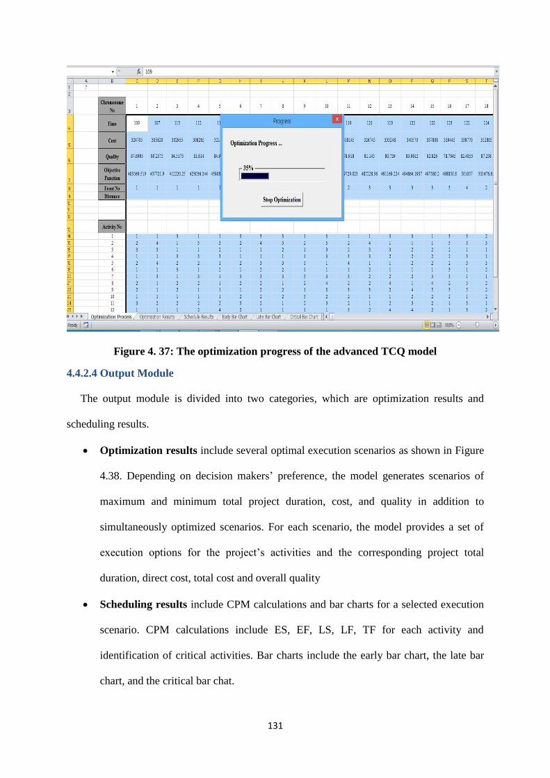
131
Figure 4. 37: The optimization progress of the advanced TCQ model
4.4.2.4 Output Module
The output module is divided into two categories, which are optimization results and
scheduling results.
Optimization results include several optimal execution scenarios as shown in Figure
4.38. Depending on decision makers’ preference, the model generates scenarios of
maximum and minimum total project duration, cost, and quality in addition to
simultaneously optimized scenarios. For each scenario, the model provides a set of
execution options for the project’s activities and the corresponding project total
duration, direct cost, total cost and overall quality
Scheduling results include CPM calculations and bar charts for a selected execution
scenario. CPM calculations include ES, EF, LS, LF, TF for each activity and
identification of critical activities. Bar charts include the early bar chart, the late bar
chart, and the critical bar chat.

132
Figure 4. 38: The optimization results of the advanced TCQ model
4.4.3 Model Implementation and Validation
To validate the advanced TCQT model, the same example of the simplified TCQ model,
introduced by El-Rayes and Kandil (2005), is analyzed. The project soft and hard deadline
are set 110 and 140 respectively. The project indirect cost is assumed 1500 $/day, a penalty
of 2000 $ per each delay day after 110 days is assumed, and no incentives is considered. The
minimum acceptable overall project quality is assumed 80%. The number of population Npop
is 100 chromosomes, the number of generations is 100 iterations, the crossover rate is 0.6,
and the initial mutation rate is 0.3. For the optimization approach, the three approaches of
GP, MAWA, and NSGAII are examined. For the optimization objectives, both time-cost and
time-cost-quality are also examined.
After the user enters the problem data, it is stored in a hidden sheets as shown in Figures
4.39 to 4.41. Figure 4.39 shows the scheduling and precedence data of the example, Figure
4.40 shows the cost and duration data of execution options for each activity, Figure 4.41
shows the quality data of the example including weights of activities, weights of quality
indicators, and performance of each execution option in such quality indicators. After the
optimization process is completed, optimum solutions are generated as shown in Figure 4.42.

133
Figure 4. 39: The scheduling data of the advanced TCQ model

134
Figure 4. 40: The duration and cost of execution options of the advanced TCQ model

135
Figure 4. 41: The quality data of the advanced TCQ model

136
Figure 4. 42: The optimization output of the advanced TCQ model

137
For the output module, the user selects an execution scenario that provides an execution
option for each activity within the project, the total project cost, duration, and quality for that
selected scenario as shown in Figure 4.43. By pressing the CPM calculations button, the
schedule results are computed as shown in Figure 4.44. The early, late, and critical bar
buttons are used to generate the early, late, and critical bar charts of Figures 4.45 to 4.47.
Figure 4. 43: Optimization results for a selected scenario of the advanced TCQ model

138
Figure 4. 44: Scheduling results for a selected scenario of the advanced TCQ model
Figure 4. 45: Early bar chart for a selected scenario of the advanced TCQ model

139
Figure 4.46: Late bar chart for a selected scenario of the advanced TCQ model
Figure 4. 47: Critical bar chart for a selected scenario of the advanced TCQ model

140
4.4.4 Results and Analysis
Tables 4.11 to 4.16 show the advanced TCQ model results for various optimization
approaches and various optimization objectives. The following conclusions were reached by
the generated results:
Compared to results that obtained by literature, (Hegazy & Ayed, 1999), (El-Rayes &
Kandil, 2005), and (Zheng et al. , 2004), satisfactory results were obtained by the
advanced TCQ model.
Compared to results of the simplified TCQ model utilizing the Evolver add-in,
comparable results were obtained by the advanced TCQ model utilizing the self-
developed optimization tool.
It is obvious that the NSGAII approach outperforms the other two approaches in
analyzing both TCT and TCQT problems.
Tables 4.11 and 4.14 demonstrate the impact of objectives’ weights of the GP
approach on the obtained solutions. Therefore, it is recommended to apply the GP
approach when there is a prefrernce for a specific objective.
Based on conducted tests and according to the developed code, it is recommended to
set the population size between 50 and 100 and the number of generations between
100 and 200. It is recommended to set the crossover rate between 0.4 and 0.6 and the
initial mutation rate between 0.05 and 0.3.
For the MAWA approach, it is recommended to reduce the initial mutation rate (Pmi)
in order no to disrupt the produced offspring solutions. Pmi of 0.05 generates
satisfactory solutions.
Scheduling results provided by the advanced TCQT model were compared with
results produced by MS Project and both were identical.

141
Table 4.11: The GP approach results of the advanced TCQ model
Table 4.12: The MAWA approach results of the advanced TCQ model
Table 4.13: The NSGAII approach results of the advanced TCQ model
Table 4.14: The GP approach results of the advanced TCQ model for TCT
Weights of Objectives
The GP Approach Results
Solution
Direct
Cost
Total
Duration
Total
Cost
Total
Quality
Execution options for activities
Wt Wc Wq 1 2 3 4 5 6 7 8 9 10 11 12 13 14 15 16 17 18
1 1 0 0 104 163,470 319,470 88.95 1 3 3 1 1 1 1 5 1 1 3 1 2 3 1 2 1 1
2 0 1 0 108 122,320 284,320 80.11 1 3 1 3 4 2 3 5 1 1 1 1 3 1 1 5 1 1
3 0 0 1 107 168,755 329,255 97.46 1 1 1 1 1 1 1 2 2 1 1 1 1 1 1 1 1 1
4 0.333 0.333 0.333 104 150,320 306320 92.62 1 1 1 3 2 1 1 1 1 1 1 1 1 1 1 2 1 1
Weights of ObjectivesSolution
Direct
Cost
Total
Duration
Total
Cost
Total
Quality
Execution options for activities
The MAWA Approach Results
Solution
Total
Duration
Direct
Cost
Total
Cost
Total
Quality
Execution options for activities
1 2 3 4 5 6 7 8 9 10 11 12 13 14 15 16 17 18
1 104 161,015 317,015 91.63 1 2 2 1 1 1 2 2 1 1 2 1 1 2 1 1 1 1
2 107 151340 311840 89.71 1 4 1 3 1 1 1 3 2 1 2 1 1 3 1 1 1 1
3 104 145,115 301,115 86.81 1 4 2 3 1 1 2 2 1 1 2 1 1 2 1 1 1 1
4 106 155,070 314070 87.54 1 2 2 1 1 1 3 5 1 1 1 2 3 2 1 4 1 1
Solution
Total
Duration
Direct
Cost
Total
Cost
Total
Quality
Execution options for activities
The NSGAII Approach Results
Solution
Total
Duration
Direct
Cost
Total
Cost
Total
Quality
Execution options for activities
1 2 3 4 5 6 7 8 9 10 11 12 13 14 15 16 17 18
1 108 122,400 284,400 80.25 1 3 1 3 4 2 3 3 1 1 1 1 3 1 1 5 1 1
2 104 162820 318820 95.16 1 1 1 1 1 1 2 1 1 1 1 1 1 1 1 1 1 1
3 104 150,320 306,320 92.62 1 1 1 3 2 1 1 1 1 1 1 1 1 1 1 2 1 1
4 104 141,100 297100 88.67 1 3 1 3 2 1 3 3 1 1 1 1 1 1 1 2 1 1
5 104 149,820 305820 92.2 1 1 1 3 2 1 1 1 1 1 1 1 1 1 1 4 1 1
6 104 168,820 324820 97.63 1 1 1 1 1 1 1 1 1 1 1 1 1 1 1 1 1 1
Solution
Total
Duration
Direct
Cost
Total
Cost
Total
Quality
Execution options for activities
Wt Wc 1 2 3 4 5 6 7 8 9 10 11 12 13 14 15 16 17 18
1 1 0 104 152,858 308,858 1 5 2 2 1 1 1 4 1 1 1 1 3 1 1 3 1 1
2 0 1 108 119,270 281,270 1 5 3 3 4 2 3 5 1 1 3 1 3 3 1 5 1 1
3 0.5 0.5 105 127,270 284,770 1 5 3 3 4 1 3 5 1 1 3 1 3 3 1 5 1 1
The GP Approach Results for TCT
SolutionWeights of Objectives Total
Duration
Direct
Cost
Total
Cost
Execution options for activities

142
Table 4.15: The MAWA approach results of the advanced TCQ model for TCT
Table 4.16: The NSGAII approach results of the advanced TCQ model for TCT
4.4.5 Model Capabilities and Limitations
Results of the application example supports the utilization of the advanced TCQ model in
various TCQT and TCT problems due to its effectiveness and efficiency. Capabilities and
limitations of the advanced TCQ model are as follows:
4.4.4.1 Capabilities and Strengths of the Advanced Model
Quality performance evaluation approach for both the activity level and project level.
Generalized dependency relationships among activities.
The ability to enter up to five execution options for each activity.
The ability to enter up to five successors and predecessors for each activity.
Three various MOO approaches are available.
Generation of several optimal solutions rather than one solution to provide decision
makers with alternatives to choose from depending on their preference.
The ability to analyze time-cost optimization problems in addition to time-cost-quality
optimization problems.
Robust results with adequate processing time considering the large search space
1 2 3 4 5 6 7 8 9 10 11 12 13 14 15 16 17 18
1 104 140,700 296,700 1 4 1 3 3 1 2 3 1 1 1 1 1 2 1 1 1 1
2 107 130,920 291,420 3 1 3 3 4 1 2 5 1 1 1 1 3 3 1 5 1 1
3 106 136,170 295,170 3 4 1 3 3 1 2 1 1 1 3 1 3 3 1 4 1 1
SolutionTotal
Duration
Direct
Cost
Total
Cost
Execution options for activities
The MAWA Approach Results for TCT
1 2 3 4 5 6 7 8 9 10 11 12 13 14 15 16 17 18
1 104 132,270 288,270 1 5 3 3 3 1 3 5 1 1 3 1 3 3 1 5 1 1
2 108 119,270 281,270 1 5 3 3 4 2 3 5 1 1 3 1 3 3 1 5 1 1
3 105 127,270 284,770 1 5 3 3 4 1 3 5 1 1 3 1 3 3 1 5 1 1
The NSGAII Approach Results for TCT
SolutionTotal
Duration
Direct
Cost
Total
Cost
Execution options for activities

143
Spreadsheet features and capabilities associated with developing the models in MS
Excel.
Ease of use and simplicity.
Error handling messages to guide the model user.
4.4.4.2 Limitations and Weaknesses of the Advanced Model
Premature conversion of the GP and MAWA optimization approaches
Complexity of data entry for large-scale projects
Excessive processing time for large-scale projects
Uncertainty is not considered
4.5 Summary
Three various TCQT models were developed in order to optimize the performance of
construction projects in terms of total duration, total cost, and overall quality. The main goal
of those three developed models is to optimize the utilization of execution options in order to
select an option for each activity within the project to satisfy decision makers’ objectives. A
simplified TCQ model utilizing the Evolver add in was developed to analyze simple projects
with maximum three resource execution options and only finish to start dependency
relationships. A stochastic TCQ model capable of considering uncertainty associated with
execution options’ performance and the whole project’s performance with regard to time,
cost, and quality was developed to analyze stochastic problems. Moreover, an advanced TCQ
model utilizing a self-developed MOO tool was developed. In addition to TCQT analysis, the
advanced TCQ model was applied to a TCT analysis and results were satisfactory.

144
Chapter V: Conclusion
The main objective of any construction project is to finish the project within an estimated
budget, according to a pre-specified level of quality, and without any delays. Therefore, the
total duration, cost, and quality of construction projects are of great importance for
contractors and project managers. Time-cost optimization or TCT is considered one of the
most important features of projects’ planning and controlling. The main idea of time-cost
trade-off is to strike a balance between the decreased indirect costs and the increased direct
costs associated with accelerating projects. Owners, consultants, and general contractors
should consider quality of work proposed by each subcontractor or execution option in order
to make accurate decisions related to execution of construction projects. It is required to
determine an optimal or near optimal trade-off among cost, time and quality of construction
projects, which means to complete the project at a given deadline or with minimum duration,
provided that its total cost is minimized and its overall quality is maximized.
5.1 Conclusions
The main idea of TCQT is to strike a balance among the conflicting objectives of time,
cost and quality. There are two categories of trade-off problems: (1) continuous trade off
problems, in which the relation among time, cost, and quality has been considered a
continuous function; (2) discrete trade-off problems, in which the relation among time, cost,
and quality has been considered discrete or isolated. Discrete time-cost-quality relationships
are preferred for two main reasons: (1) it is more relevant to real world construction projects;
(2) it is suitable for modeling any general time-cost relationship (Tareghian & Taheri, 2006).
For optimization techniques, evolutionary algorithms are preferable and commonly used
because they can deal with more than one objective, easily achieve diverse solutions, and
they are more effective when applied to large-scale problems. Amongst various EA
techniques, GA has been extensively utilized for optimization problems in general and

145
construction management problems in particular. Multi-objective optimization approaches
have been also reviewed. Three approaches of MOO techniques have been discussed, which
are goal programming (GP), Pareto optimum, and non-dominated sorting genetic algorithm
(NSGA-II). The NSGA-II has demonstrated to be one of the most robust algorithms for MOO
problems.
Three TCQT models were developed in MS Excel: the simplified model to optimize the
objectives of time, cost, and quality of simple projects; the stochastic model to analyze
projects considering uncertainty; and the advanced model to analyze both TCT and TCQT for
large-scale projects. The main objective of such models is to find an optimal or near optimal
set of execution options for a project’s activities in order to minimize the project’s total cost,
minimize its total duration, and maximize its overall quality. The Evolver add-in software
was utilized as an optimization tool for the first two models; however, a self-developed
optimization tool utilizing three various optimization approaches was utilized for the
advanced model. To validate the developed models and demonstrate their efficiency, they
were applied to case studies introduced by literature. Compared to results obtained by
literature, satisfactory results were obtained by the developed models. In addition, the
advanced TCQ model utilizing the self-developed optimization tool generated comparable
results compared to those obtained by the Evolver add-in.
5.2 Research Contributions
This research contributes to improve controlling and planning of construction projects. It
facilitates the process of decision making with regards to the duration, cost, and quality of
projects. It helps decision makers to select the most appropriate execution options to
complete the work of construction projects’ activities. The main contributions of this research
can be summarized as follows:

146
Adequate illustration of existing optimization approaches. This study provided an in-
depth review of optimization approaches such as heuristic, mathematical, and
evolutionary approaches.
Extensive review of approaches and methodologies utilized to analyze TCT and TCQ
problems.
Investigating recent MOO techniques and the most effective ones were utilized by the
developed models.
Investigating quality measurement approaches and the most appropriate ones were
incorporated into the developed TCQ models.
The need for incorporating uncertainty when controlling and scheduling construction
projects was outlined.
The utilization of the Evolver add in as a powerful optimization tool is outlined.
Development of a simplified TCQ model used for simple construction projects.
Development of a stochastic TCQ model to consider uncertainty associated with
execution options and the whole project performance.
Development of a powerful advanced TCQ model capable of simultaneously
minimizing the total project cost and duration, while maximizing the overall project
quality.
Application of three various MOO approaches to be utilized by the advanced TCQ
model and TCQT problems in general.
Development a MS Excel based scheduling tool capable of scheduling problems with
generalized dependency relationships.

147
5.3 Future Research
Despite the simplicity of the developed models and robustness of their obtained results,
various other enhancements and improvements are recommended for further extensions of the
current research. The following areas are instances of recommendations for future research:
Utilizing other recent optimization packages such as C-Plex, solver platform, or
Quantum.
Incorporating fuzzy sets or Monte Carlo Simulation to consider uncertainty associated
with construction projects in studying the TCQT analysis problems.
Research on the indicators that affect the quality of execution options of activities in
construction projects. Research on activity weights with in different categories of
construction projects.
Incorporating a fourth objective into the optimization process such as increasing
safety or reducing risk.
Incorporating Resource utilization optimization into the model; resource allocation
and resource leveling constraints.
Integration between the optimization model and commercial software such as
primavera or MS Project.

148
Bibliography AACE International . (2004). Skills & Knowledge of Cost Engineering. Morgantown: AACE
International– the Association for the Advancement of Cost Engineering.
AACE International – the Association for the Advancement of Cost Engineering. (2004). Skills &
Knowledge of Cost Engineering. Morgantown: AACE International.
Abd El Razek, R., Diab, A., Hafez, S., & Aziz, R. (2010). Time-Cost-Quality Trade-off Software by using
Simplified Genetic Algorithm for Typica-lrepetitive Construction Projects. World Academy of
Science, Engineering and Technology, 61, 312-321.
Abdel-Razek, R. (1998). Factors Affecting Construction Quality in Egypt: Identification and Relative
Importance. Engineering, Construction and Arcitectural Management, 5(3), 220-227.
Adeli, H., & Karim, A. (1997). Scheduling/Cost Optimization and Neural Dynamics Model for
Construction. Construction Engineering and Management, 123(4), 450-458.
Afshar, A., Kaveh, A., & Shoghli, O. (2007). Multi-Objective Optimization of Time-Cost-Quality Using
Multi-Colony Algorithm. Asian Journal of Civil Engineering (Building and Housing), 8(2), 113-
124.
Al-Tabtabai, H., & Alex, A. P. (1999). Using Genetic Algorithms to Solve Optimization Problems in
Construction. Engineering, Construction and Management, 6(2), 121-132.
Anderson, S., & Russell, J. (2001). Guidelines for Warranty,Multi-Parameter, and Best Value
Contracting. Washington, D.C.: National Cooperative Highway Research Program.
Assadipour, G., & Iranmanesh, H. (2010). The Discrete Time Cost and Quality Trade-off Problem in
Scheduling: An Efficient Solution Method Based on Cellde Algorithm. South African Journal of
Industrial Engineering, 21(1), 93-101.
Attalla, M., Hegazy, T., Fetaiha, A., & Elbeltagi, E. (2003). Delivering Projects with Quality and Safety.
5th Construction Specialty Conference of the Canadian Society for Civil Engineering. Toronto:
ASCE.
Awadallah, S. E. (2014). TIME-COST-QUALITY-ENVIRONMENTAL TRADE-OFF OPTIMIZATION IN
HIGHWAY CONSTRUCTION. Thesis Abstract. Zagazig, Egypt: Zagazig University.
Babu, A., & Suresh, N. (1996). Project management with time, cost, and quality considerations.
Journal of Operational Research, 88(2), 320-327.
Bingol, B., & Polat, G. (2015). Time-Cost-Quality Trade-Off Model for Subcontractors Selection Using
Discrete Particle Swarm Optimization Algorithm. Annual Association of Researchers in
Construction Management, (pp. 13-22). Lincoln, UK.
Chassiakos, A., & Sakellaropoulos, S. (2005). Time-Cost Optimization of Construction Projects with
Generalized Activity Constraints. Construction Engineering and Management, 131(10), 1115-
1124.

149
Cristóbal, J. (2009). Time, Cost, and Quality in a Road Building Project. Journal of Construction
Engineering and Management, Vol. 135, No. 11, November 1, 2009., 135(11), 1271-1274.
Deb , K., Prata, A., Agarwal, S., & Meyarivan, T. (2002). A Fast and Elitist Multiobjective Genetic
Algorithm: NSGA-II. IEEE Transactions on Evolutionary Computation, 6(2), 182-197.
Deb, K. (2001). Multi-Objective Optimization using Evolutionary Algorithms. Chichester: John Wiley &
Sons Ltd.
Diao, X., Li, H., Guo, H., Zeng, S. X., & Wy Ta, V. (2011). A Pareto Multi-Objective Optimization
Approach for Solving Time-Cost-Quality Tradeoff Problems. Technological and Economic
Development of Economy, 17(1), 22-41.
Elazouni, A., & Metwally, F. (2005). Finance-Based Scheduling: Tool to Maximize Project Profit Using
Improved Genetic Algorithms. Construction Engineering and Management, 131(4), 400-412.
Elazouni, A., & Metwally, F. (2007). Expanding Finance-Based Scheduling to Devise Overall-Optimized
Project Schedules. Construction Engineering and Management, 133(1), 86-90.
Elbeltagi, E., Hegazy, T., & Grieson, D. (2005). Comparison among Five Evoltionary-Based
Optimization Algorithms. Advanced Engineering Informatics, 19, 43-53.
Ellis, R. (1990). Estimating the cost of construction inspection. The American Association of Cost
Engineers.
El-Rayes, K., & Kandil, A. (2005). Time-Cost-Quality Trade-Off Analysis for Highway Construction.
Construction Engineering and Management, 131(4), 477-486.
Ezeldin, S., & Soliman, A. (2009). Hybrid Time-Cost Optimization of Nonserial Repetitive Construction
Projects. Construction Engineering and Management, 135(1), 42-55.
Fang, F., & Zhang, C. (2014). A New Approach to Time-Cost-Quality Tradeoff Problem for
Construction Project. International Conference on Management Science & Engineering
(21th), (pp. 1836-1842). Helsinki, Finland.
Feng, C.-W., Liu, L., & Burns, S. (1997). Using Genetic Algorithms to Solve Construction Time-Cost
Trade-Off Problems. Computing in Civil Engineering, 11(3), 184-189.
Feng, C.-W., Liu, L., & Burns, S. (2000). Stochastic Construction Time-Cost Trade-Off Analysis.
Computing in Civil Engineering, 14(2), 117-126.
Geem, Z. W. (2010). Multiobjective Optimization of Time-Cost Trade-Off Using Harmony Search.
Construction Engineering and Management, 136(6), 711-716.
Ghodsi, R., Skandari, M., Allahverdiloo, M., & Iranmanesh, S. (2009). A New Practical Model to Trade-
off Time, Cost, and Quality of a Project. Australian Journal of Basic and Applied Sciences,
3(4), 3741-3756.
Haidar, A., Naoum, S., Howes, R., & Tah, J. (1999). Genetic Algorithms Application and Testing for
Equipment Selection. Construction Engineering and Management, 32-38.

150
Hegazy, T. (2002). Computer-Based Construction Project Management. Ontario: Prentice Hall.
Hegazy, T. (2006). Simplified Project Management for Construction Practitioners. Cost Engineering,
48(11), 20-28.
Hegazy, T., & Ayed, A. (1999). Simplified Spreassheet Solutions: Models for Critical Path Method and
Time-Cost Trade-off analysis. Cost Engineering, 41(7), 26-33.
Hegazy, T., & Ersahin, T. (2001). Simplified Spreadsheet Solutions: Overall Schedule Optimization.
Construction Engineering and Management, 127(6), 469-475.
Hegazy, T., & Menesi, W. (2010). Critical Path Segments Scheduling Technique. Construction
Engineering and Management, 136(10), 1078-1085.
Hegazy, T., & Wassef, N. (2001). Cost Optimization in Projects with Repetitive Nonserial Activities.
Construction Engineering and Management, 127(3), 183-191.
Heravi, G., & Faeghi, S. (2014). Group Decision Making for Stochastic Optimization of Time, Cost, and
Quality in Construction Projects. Journal of Computing in Civil, 28(2), 275-283.
Hinze, J. W. (2004). Construction Planning and Scheduling. New Jersey: Pearson Prentice Hall.
Huimin, L., & Zhuofu, W. (2009). Memetic Algorithm for Solving Construction Time-Cost
Optimization. Management and Service Science, 2009. MASS '09, (pp. 1-4). Wuhan.
Iranmanesh, H., Skandari, M., & Allahverdiloo, M. (2008). Finding Pareto Optimal Front for the Multi-
Mode Time, Cost Quality Trade-off in Project Scheduling. World Academy of Science,
Engineering and Technology, 40, 346-350.
Kandil, A., & El-Rayes, K. (2006a). Parallel Genetic Algorithms for Optimization Resource Utilization in
Large-Scale Projects. Construction Engineering and Management, 132(5), 491-498.
Kandil, A., & El-Rayes, K. (2006b). MACROS: Multiobjective Automated Construction Resource
Optimization System. Journal of Management in Engineering, 22(3), 126-134.
Kandil, A., El-Rayes, K., & El-Anwar, O. (2010). Optimization Research: Enhancing the Robustness of
Large-Scale Multiobjective Optimization in Construction. Construction Engineering and
Management, 136(1), 17–25.
Kerzner, H. (2009). Project Management : a System Approach to Planning, Scheduling, and
Controlling. New York: John Wiley & Sons, Inc.
Khalafallah, A., & El-Rayes, K. (2006). Minimizing Construction-Related Hazarads in Airport Expansion
Projects. Construction Engineering and Management, 132(6), 562-572.
Khang, D. B., & Myint, Y. M. (1999). Time, cost and quality trade-off in project management: a case
study. International Journal of Project Management, 17(4), 249-256.
Li, H., & Love, P. (1997). Using Imroved Genetic Algorithms to facilitate Time Cost Optimization.
Construction Engineering and Management, 123(3), 233-237.

151
Liu, L., Burns, S., & Feng, C.-W. (1995). Construction Time-Cost Trade-Off Analysis using LP/IP Hybrid
Method. Construction engineering and Management, 121(4), 446-454.
Ma, W.-m., LIU, Q.-H., & KE, H. (2014). A Stochastic Time-cost-quality Tradeoff Model for Discrete
Project Scheduling Problem. International Conference on Management Science and
Management Innovation (pp. 318-323). Changsha, China: Atlantis Press.
MADANY, M., MARZOUK, M., ABOU-ZIED, A., & EL-SAID, M. (2009). TIME-COST-QUALITY-POLLUTION
TRADE-OFF ANALYSIS FOR CONSTRUCTION PROJECTS. Thirteenth International Conference
on Structural and Geotechnical Engineering (pp. 201-212). Cairo: Ain Shams University.
Marzouk, M., & Moselhi, O. (2002). Simulation Optimization for Earthmoving Operations Using
Genetic Algorithms. Construction Management and Economics, 20, 535-543.
Montgomery, D. C. (2003). Applied Statistics and Probability for Engineers. New York: John Wiley &
Sons, Inc.
Montgomery, D., & Runger, G. (2003). Applied Statistics and Probability for Engineers (3rd ed.). New
York: John Wiley & Sons, Inc.
Ng, T., & Zhang, Y. (2008). Optimizing Construction Time and Cost Using Ant Colony Optimization
Approach. Construction Engineering and Management, 134(9), 721–728.
O'Braien, J. (1989). Construction Inspection Handbook: Quality Assurance/Quality Control. New York:
Van Nostrand Reinhold.
Palisade Corporation. (2010). Guide to Using Evolver: The Genetic Algorithm Solver for Microsoft
Excel. New York: Palisade Corporation.
Pollack-Johnson, B., & Liberatore, M. (2006). Incorporating Quality Considerations Into Project
Time/Cost Tradeoff Analysis and Decision Making. IEEE Transactions on Engineering
Management, 53(4), 534-542.
Pour, N. S., Modarres, M., & Tavakkoli-Moghaddam, R. (2012). Time-Cost-Quality Trade-off in Project
Scheduling with Linguistic Variables. World Applied Sciences, 18(3), 404-4013.
Pour, S., Modarres, M., Aryanejad, M., & Moghadam, T. (2010). The Discrete Time-Cost-Quality
Trade-off Problem Using a Novel Hybrid Genetic Algorithm. Applied Mathematical Sciences,
4(42), 2081-2094.
Project Management Institute (PMI). (2008). A Guide to the Project Management Body of Knowledge
(Vol. 4th Edition). Pennsylvania, USA: PMI.
Que, B. C. (2002). Incorporating Practicability into Genetic Algorithm-Based Time-Cost Optimization.
Construction Engineering and Management, 128(2), 139–143.
Rahimi, M., & Iranmanesh, H. (2008). Multi Objective Particle Swarm Optimization for a Discrete
Time,Cost and Quality Trade -off Problem. World Applied Sciences, 4(2), 270-276.
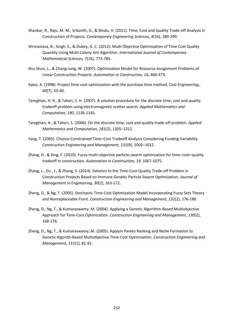
152
Shankar, R., Raju, M. M., Srikanth, G., & Bindu, H. (2011). Time, Cost and Quality Trade-off Analysis in
Construction of Projects. Contemporary Engineering Sciences, 4(16), 289-299.
Shrivastava, R., Singh, S., & Dubey, G. C. (2012). Multi Objective Optimization of Time Cost Quality
Quantity Using Multi Colony Ant Algorithm. International Journal of Contemporary
Mathematical Sciences, 7(16), 773-784.
Shu-Shun, L., & Chang-Jung, W. (2007). Optimization Model for Resource Assignment Problems of
Linear Construction Projects. Automation in Construction, 16, 460-473.
Sipos, A. (1998). Project time-cost optimization with the purchase time method. Cost Engineering;,
40(7), 33-40.
Tareghian, H. R., & Taheri, S. H. (2007). A solution procedure for the discrete time, cost and quality
tradeoff problem using electromagnetic scatter search. Applied Mathematics and
Computation, 190, 1136-1145.
Tareghian, H., & Taheri, S. (2006). On the discrete time, cost and quality trade-off problem. Applied
Mathematics and Computation, 181(2), 1305–1312.
Yang, T. (2005). Chance-Constrained Time–Cost Tradeoff Analysis Considering Funding Variability.
Construction Engineering and Management, 131(9), 1002–1012.
Zhang, H., & Xing, F. (2010). Fuzzy-multi-objective particle swarm optimization for time–cost–quality
tradeoff in construction. Automation in Construction, 19, 1067-1075.
Zhang, L., Du , J., & Zhang, S. (2014). Solution to the Time-Cost-Quality Trade-off Problem in
Construction Projects Based on Immune Genetic Particle Swarm Optimization. Journal of
Management in Engineering, 30(2), 163-172.
Zheng, D., & Ng, T. (2005). Stochastic Time-Cost Optimization Model Incorporating Fuzzy Sets Theory
and Nonreplaceable Front. Construction Engineering and Management, 131(2), 176-186.
Zheng, D., Ng, T., & Kumaraswamy, M. (2004). Applying a Genetic Algorithm-Based Multiobjective
Approach for Time-Cost Optimization. Construction Engineering and Management, 130(2),
168-176.
Zheng, D., Ng, T., & Kumaraswamy, M. (2005). Applyin Pareto Ranking and Niche Formation to
Genetic Algorith-Based Multiobjective Time-Cost Optimization. Construction Engineering and
Management, 131(1), 81-91.