Time-based Competition with Benchmark Effects

Liu Yang Francis de Vericourt Peng Sun

May 9, 2012

Abstract

We consider a duopoly where firms compete on waiting times in the presence

of an industry benchmark. The demand captured by a firm depends on the gap

between the firm’s offer and the benchmark. We refer to the benchmark effect as

the impact of this gap on demand. The formation of the benchmark is endoge-

nous and depends on both firms’ choices. When the benchmark is equal to the

shorter of the two offered delays, we characterize the unique Pareto Optimal Nash

equilibrium. Our analysis reveals a stickiness effect by which firms equate their

delays at the equilibrium when the benchmark effect is strong enough. When the

benchmark corresponds to the average of the two offered delays, we show the exis-

tence of a pure Nash equilibrium. In this case, we reveal a reversal effect, by which

the market leader, in terms of offered shorter delay, becomes the follower when

the benchmark effect is strong enough. In both cases, we show that customers

benefit when an industry benchmark exists because equilibrium waiting times are

shorter. Our models also capture customers’ loss aversion, which, in our setting,

states that demand is more sensitive to the gap when the delay is longer than the

benchmark (loss) rather than shorter (gain). We characterize the impact of this

loss aversion on the equilibrium in both settings.

Keywords: Waiting Time Competition, Benchmark Effect, Loss Aversion,

Queues, Game Theory

1

1 Introduction

Service firms often compete on waiting times (see Allon and Federgruen (2007) and

references therein). In this classical context, a firm adjusts the expected delay it offers to

the market in order to attract additional demands so as to maximize profit. Customers,

in turn, derive their utility from the waiting time they experience at the firm they

choose to join. However, customer satisfaction may also directly depend on other offers

in the competition. For instance, a given level of delay can be more or less dissatisfying

depending on whether it is longer or shorter than some industry benchmark. This is

because customers are subject to reference effects (Kahneman and Tversky 1979) when

evaluating waiting times (Leclerc et al. 1995) or, more generally, service quality (Cadotte

et al. 1987). When setting an expected waiting time, a firm also influences the benchmark

against which customers evaluate the delays they experience at other firms. The main

contribution of this paper is to offer a theoretical analysis on how benchmark effects

such as these influence waiting time competition between firms.

To that end, we consider a simple duopoly where firms offer expected waiting times

for their service by adjusting their service rates at a capacity cost. Demand is then split

between firms according to the different levels of customer satisfaction. More precisely,

the customer’s satisfaction at a firm is a function of both firms’ expected waiting times

as in the classical duopoly but also of the gap between the firm’s offered delay and the

benchmark. We refer to the benchmark effect as the impact the gap has on demand.

Our model also allows for customers to be loss averse, in the sense that a positive gap,

i.e. when the offered delay exceeds the benchmark, has a greater impact on satisfaction

than the corresponding negative gap, i.e. when the benchmark exceeds the delay by the

same amount. Thus, a firm’s decision has a direct effect on demand through its choice

of waiting time, and an indirect one through the benchmark effect. Following Cadotte

et al. (1987), we consider two different settings depending on how the benchmark is

formed. In the first, the benchmark equals the smaller of the two offered waiting times,

while in the second, the benchmark corresponds to the average. Without the benchmark

effect, our model corresponds to a classical set-up of time-based competition.

This situation gives rise to a game in which each firm strategically chooses a waiting

2

time in order to maximize profit. We show the existence of and characterize the Nash

equilibriums for this problem. We find that the presence of a benchmark benefits cus-

tomers, in the sense that customers experience shorter delays in the equilibrium with

benchmark effect compared to the classical duopoly case without benchmark. In fact,

the expected waiting times in equilibrium become smaller as the benchmark effect gets

stronger.

In our first setting, where the benchmark corresponds to the smaller expected waiting

time, our analysis reveals a stickiness effect by which firms equate their offers at the

equilibrium as long as the ratio of their profit margins belongs to a given interval. By

contrast, in the absence of the benchmark, the offered waiting times are equal only when

the ratio takes a specific value. We further show that, while the interval expands as the

benchmark effect intensifies, it may shrink or expand with the level of loss aversion

depending on whether the benchmark effect is strong enough. In other words, the

intensity of the benchmark effect changes the direction of the impact of loss aversion on

the equilibrium waiting time.

In our second setting, where the benchmark corresponds to the average waiting

time between the two firms, we identify a reversal effect in the sense that the leader

in a duopoly without benchmark effect, in terms of offering shorter waiting time, can

become the follower (offering longer waiting time) if the benchmark effect is strong

enough. The market leader is determined by a threshold on the profit-margin ratio,

which is monotone in both benchmark effect and loss aversion effects. Similar to the

minimum benchmark case, the threshold may either decrease or increase with the level

of loss aversion depending on the intensity of the benchmark effect.

The presence of a benchmark effect is supported by results of prospect theory (Kahne-

man and Tversky 1979), which demonstrates that people generally view a final outcome

as a gain or a loss with respect to a certain context-dependent reference point. While

the original applications of prospect theory mainly studied people’s preference towards

monetary payoffs (Niedrich et al. 2001, Erdem et al. 2001, Popescu and Wu 2007), em-

pirical study (Leclerc et al. 1995) demonstrates that a similar reference effect also exists

in waiting times. In our context, the service benchmark determines the waiting time

reference point. The benchmark effect corresponds then to the gap between the bench-

3

mark and the actual waiting time. In other words, customers might experience “waiting

time gain” if the actual waiting time is shorter than the benchmark, and “waiting time

loss” otherwise.

The benchmark effect is also highly consistent with the stream of research on service

quality and customer satisfaction. According to Anderson and Sullivan (1993), for in-

stance, customer satisfaction from a service is a function of perceived quality as well as

the gap between customers’ expectation (reference point) and perceived quality. More-

over, when perceived quality falls short of expectation, the gap has a greater impact

on satisfaction than the corresponding gap when quality exceeds expectation, a result

consistent to Prospect Theory’s loss aversion. Lin et al. (2008) empirically studied the

impact of the service quality gap on customers’ behavior intentions. They show that a

customer’s behavior depends on the service quality gap according to a value function

that is “kinked” at the reference point, with the loss of service quality influencing the

customer’s behavior more than does a corresponding service quality gain. This is also

consistent with prospect theory.

Empirical studies further suggest how firms’ decisions might determine together the

benchmark, i.e. the reference point (see Zeithaml et al. (1993)). For instance, Cadotte

et al. (1987) show that two types of comparisons better explain customer satisfaction

with service quality: “best brand norm” and “product type norm.” According to the

“best brand norm” case, customers select the best brand in the category as their refer-

ence. The “product type norm” case, on the other hand, represents the setting where

the average performance is perceived as typical of a group of similar brands. This case

is also consistent with the adaptation-level theory where the reference standard is per-

ceived as the mean of the stimuli presented within a contextual set (Helson 1964, Wedell

1995). In our setting, service quality corresponds to offered waiting time and, therefore,

the minimum and average delays between the two firms correspond to the best brand

and product type norms in the customer satisfaction literature, respectively.1

This work is closely related to the literature on competition between service firms

1Theoretically, the product type norm should represent the weighted average of the two firms’ waitingtimes, with the weights to be each firm’s demand rate. However, such weights are endogenous and willmake the analysis much harder. We thus use the simple average to avoid the unnecessary technicalitywhile still capturing the essence.

4

when customers are sensitive to waiting time, or service quality. Service competition has

been a subject of many studies (see Hassin and Haviv (2002) for a comprehensive review

in queueing settings). In some of these models (De Vany and Saving 1983, Kalai et al.

1992, So 2000, Cachon and Harker 2002, Ho and Zheng 2004, Allon and Federgruen

2007), firms compete in both waiting times and prices either in an aggregated form

(full price) or as separate attributes. Gaur and Park (2007), Liu et al. (2007) and Hall

and Porteus (2000), instead, consider the situations in which customers’ demand solely

depends on waiting time, or service quality. In fact, certain industries experience a

higher level of price rigidity compared to their ability to vary service rates. Blinder

et al. (1998) provides extensive empirical evidence. For example, half of the businesses

in their study change prices no more than once per year. Among all industries under

study, service companies adjust prices the most slowly. Therefore, in this paper we focus

on waiting time competition, and leave price as exogenous.

Our model is most closely related to Allon and Federgruen (2007), which investigates

service competition in both service levels and prices. In the absence of the benchmark

effect, our model corresponds to a special scenario of their “price first” case, for which our

main findings disappear. Ho and Zheng (2004) also study a similar duopoly competition

in waiting time announcements when demand is affected by service quality. The paper

studies the case where firms do not need to comply to the waiting times they offer as

Allon and Federgruen (2007) and we do. On the other hand, Ho and Zheng (2004) do

consider benchmark effects and loss aversion, the main focus of our paper.

Our paper also contributes to the emerging literature on competition between firms

with customer reference effects. Heidhues and Koszegi (2008) study price competition

when customers base their reference on their recent expectations about the product.

They have shown the existence of focal price equilibrium with the presence of the ref-

erence effect. Zhou (2011) also examines firms’ price competition, yet with customers’

reference point based more on the “prominent” firm. In this setting the equilibrium

price randomizes between high and low levels. These two papers consider price competi-

tion rather than service operations competition. They also consider exogenous reference

points while the benchmark is endogenously determined by the firms’ strategies in our

set-up.

5

The remainder of the paper is organized as follows. Section 2 presents the minimum

benchmark model and the corresponding waiting time competition game. After char-

acterizing the unique (Pareto) Nash equilibrium structure, we analyze the “stickiness”

effect of equilibrium waiting times, and how they are affected by the benchmark and

loss aversion effects. Section 3 analyzes the average benchmark model, its Nash equilib-

rium characterization and the impacts of the benchmark and loss aversion effects on the

“reversal” phenomenon. We conclude the paper and discuss future research directions

in Section 4.

2 The Minimum Benchmark Case

Consider two competing firms, each acting as an M/M/1 facility. We assume that firm

i chooses and commits to an expected waiting time wi. That is, for a given demand

arrival rate λi, firm i offers service rate µi to match the waiting time commitment

wi = 1/(µi − λi). Therefore, firm i has to offer capacity µi = λi + 1/wi. We use

subscript −i to represent the firm competing with firm i.

Empirical evidence from Cadotte et al. (1987) indicates that customers sometimes

use a “best brand norm” to form a benchmark of service quality, i.e. customers select the

best brand in the category as their benchmark. In our setting, this corresponds to the

shorter waiting time, or, r ≡ min(wi, w−i), where r denotes the waiting time benchmark.

We study the average case in the following section.

Define then s (t, r) to be the customer satisfaction when she waits t units of time.

Following the marketing literature (see, for instance, Anderson and Sullivan (1993)),

we assume that the customer satisfaction with a service depends on service quality

and the gap between a customer’s expectation and the actual service quality. In our

context, service quality corresponds to the experienced waiting time t, while customer

expectation is set by benchmark r. We can then assume that customer satisfaction is

given by s (t, r) = f1(t) + f2(r − t), where function f1 represents the direct impact of

the waiting time (the service quality), and f2 the indirect impact of the benchmark (the

gap). For simplicity, we assume that both f1 and f2 are piecewise linear functions, such

6

that

s (t, r) = −αt+

βr(r − t) , if t < r ;

βrβl(r − t) , if t ≥ r ,

where α and βr > 0 represent customers’ time sensitivity for the direct impact (f1)

and the benchmark effect (f2), respectively. On the other hand, βl > 1 captures the

level of loss aversion (Kahneman and Tversky (1979)), which, in our context, states that

customers are more sensitive to waiting times that exceed the benchmark.

We refer to Si as Firm i’s aggregate satisfaction level, which corresponds to the

expectation of si(t, r) with respect to waiting time t. In the M/M/1 queueing setting,

t follows an exponential distribution with the rate parameter 1/wi. And we have,

Si(wi, r) = Et[si(t, r)] = −αwi + βr[(r − wi)− e−r/wi (β` − 1)wi

].

Following Allon and Federgruen (2007), we assume that firm i’s demand rate λi is

affected by both customers’ aggregate satisfaction level of firm i and of firm −i in a

linear fashion:

λi = a0 + aiSi(wi, r)− a−i,iS−i(w−i, r) .

Firm i’s demand rate increases in the satisfaction level of its own customers, and de-

creases in firm −i’s satisfaction level. Parameters ai and a−i,i represent the impacts of

these two attributes. We assume that ai > a−i,i > 0, so that a firm’s own attribute has

a larger impact on its demand. Note that without the benchmark effect (βr = 0), the

demand model reduces to one of the models in Allon and Federgruen (2007). Further

following Allon and Federgruen (2007), we assume that the model parameters are such

that λi is guaranteed to be positive to keep the model simple.

Furthermore, Firm i incurs capacity cost ci per unit of service rate. The price of

the service, denoted p, is identical across both service firms. Technically, all our results

still hold when the two firms’ prices are different. Denote quantity ρi = (p − ci)/ci to

represent firm i’s profit margin. Since r = min(wi, w−i), demand rate λi also depends

on wi and w−i and we can define firm i’s profit as:

Pi(wi, w−i) ≡ ci

(ρiλi(wi, w−i)−

1

wi

). (1)

7

Firm i’s objective is then to choose wi in order to maximize Pi(·, w−i).

The following proposition reveals important properties of profit function Pi, which

will prove useful to analyzing and providing insight into the competition between the

two firms.

Proposition 1. Firm i’s profit Pi, defined in Eq. (1), has the following two structural

properties:

1. Pi is a quasi-concave function of waiting time wi; and

2. Pi is supermodular when wi > w−i, and submodular when wi < w−i.

Proof. See Appendix A

The idea of the proof for quasi-concavity is as follows. We first show that firm i’s

profit Pi is concave in wi when wi ≥ w−i, and quasi-concave in wi when wi < w−i. Hence

Pi can be reduced to the four cases shown in Figure 1. In all cases but case (4), Pi is

quasi-concave. Furthermore, we show that if the left derivative of Pi with respect to wi

at wi = w−i is negative, then the right derivative cannot be positive, so that case (4) is

not possible.

As for the supermodularity and submodularity properties, when wi > w−i, increas-

ing w−i lowers customers’ expectations, making them easier to satisfy. This provides

incentive for firm i to extend its waiting time wi, which leads to the supermodularity

of Pi. On the other hand, when wi < w−i, the increase of w−i makes firm −i look even

worse, and thus increases firm i’s demand. This makes it more affordable for firm i to

lower its waiting time wi, which leads to the submodularity of Pi.

2.1 Nash Equilibrium

Given the choice of the other firm, each firm set its waiting time so as to maximize its

profit. Because demands and hence profits depend on both firm decisions, the situation

gives rise to a game. In the following, we show the existence of and fully characterize

the Nash equilibrium for this game.

Using Proposition 1, we first study firm i’s best response curve as a function of w−i.

The quasi-concavity of Pi implies that the first-order condition is a sufficient condition

8

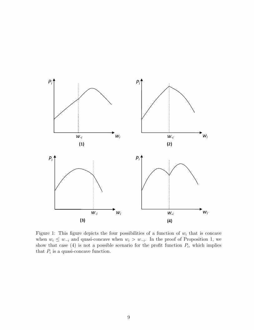
Figure 1: This figure depicts the four possibilities of a function of wi that is concavewhen wi ≤ w−i and quasi-concave when wi > w−i. In the proof of Proposition 1, weshow that case (4) is not a possible scenario for the profit function Pi, which impliesthat Pi is a quasi-concave function.

9

for firm i’s best response. However, since r = min(wi, w−i), firm i’s demand function λi

is not differentiable at wi = w−i. Nonetheless, we can define the left and right derivatives

of λi with respect to wi when wi = w−i, respectively, as

δi ≡ −∂λi∂wi

∣∣∣∣wi↑w−i

=[aiα + a−i,iβr + (ai + a−i,i)e

−1βr(βl − 1)],

δi ≡ −∂λi∂wi

∣∣∣∣wi↓w−i

=[aiα + aiβr + 2aie

−1βr(βl − 1)].

Partial derivatives δi and δi represent the impact of waiting time decision wi to arrival

rate λi, when wi approaches the competitor’s decision w−i from below and above, respec-

tively. Clearly, δi < δi when βr > 0, which means that the marginal demand increase

from setting a shorter waiting time is smaller than the marginal demand decrease from

setting a longer waiting time. Given these two quantities, firm i’s best response curve

is determined by the following Proposition:

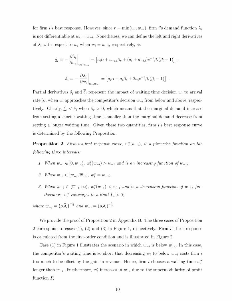
Proposition 2. Firm i’s best response curve, w?i (w−i), is a piecewise function on the

following three intervals:

1. When w−i ∈ [0, w−i), w?i (w−i) > w−i and is an increasing function of w−i;

2. When w−i ∈ [w−i, w−i], w?i = w−i;

3. When w−i ∈ (w−i,∞), w?i (w−i) < w−i and is a decreasing function of w−i; fur-

thermore, w?i converges to a limit Li > 0;

where w−i =(ρiδi)− 1

2 and w−i = (ρiδi)− 1

2 .

We provide the proof of Proposition 2 in Appendix B. The three cases of Proposition

2 correspond to cases (1), (2) and (3) in Figure 1, respectively. Firm i’s best response

is calculated from the first-order condition and is illustrated in Figure 2.

Case (1) in Figure 1 illustrates the scenario in which w−i is below w−i. In this case,

the competitor’s waiting time is so short that decreasing wi to below w−i costs firm i

too much to be offset by the gain in revenue. Hence, firm i chooses a waiting time w?i

longer than w−i. Furthermore, w?i increases in w−i due to the supermodularity of profit

function Pi.

10

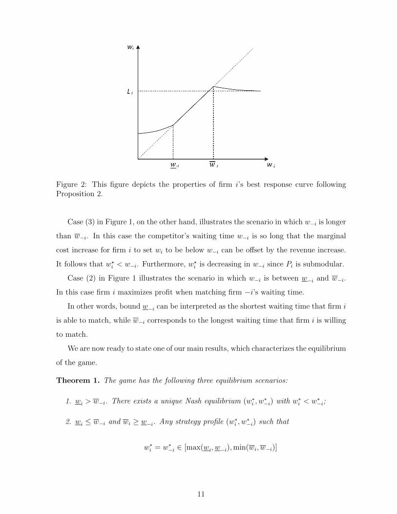
Figure 2: This figure depicts the properties of firm i’s best response curve followingProposition 2.

Case (3) in Figure 1, on the other hand, illustrates the scenario in which w−i is longer

than w−i. In this case the competitor’s waiting time w−i is so long that the marginal

cost increase for firm i to set wi to be below w−i can be offset by the revenue increase.

It follows that w?i < w−i. Furthermore, w?i is decreasing in w−i since Pi is submodular.

Case (2) in Figure 1 illustrates the scenario in which w−i is between w−i and w−i.

In this case firm i maximizes profit when matching firm −i’s waiting time.

In other words, bound w−i can be interpreted as the shortest waiting time that firm i

is able to match, while w−i corresponds to the longest waiting time that firm i is willing

to match.

We are now ready to state one of our main results, which characterizes the equilibrium

of the game.

Theorem 1. The game has the following three equilibrium scenarios:

1. wi > w−i. There exists a unique Nash equilibrium (w∗i , w∗−i) with w∗i < w∗−i;

2. wi ≤ w−i and wi ≥ w−i. Any strategy profile (w∗i , w∗−i) such that

w∗i = w∗−i ∈ [max(wi, w−i),min(wi, w−i)]

11

is a Nash equilibrium. In particular,

w∗i = w∗−i = min(wi, w−i)

is the Pareto Nash equilibrium;

3. wi < w−i. There exists a unique Nash equilibrium (w∗i , w∗−i) with w∗i > w∗−i.

Proof. The quasi-concavity of Pi implies that there exists a pure strategy Nash equilib-

rium (Fudenberg and Tirole 1991). The first two scenarios presented in Theorem 1 are

illustrated in Figures 3 and 4.

The scenario with wi > w−i corresponds to Figure 3. Given that w∗i (w−i) decreases

in w−i when w−i > w−i and is bounded below by a positive lower bound, while w∗−i(wi)

increases in wi when wi < wi, there exists a unique Nash equilibrium (w∗i , w∗−i) with

strategy profile w∗i < w∗−i, which can be characterized by the following first order condi-

tions: (p− ci)[aiα + aie

−1βr (β` − 1) + a−i,iβr(1 + e−w

∗i /w

∗−i (β` − 1)

)]= ci/w

∗2i ,

(p− c−i)[a−iα + a−iβr + a−ie

−w∗i /w

∗−iβr (β` − 1)

(1 + w∗i /w

∗−i)]

= c−i/w∗2−i .

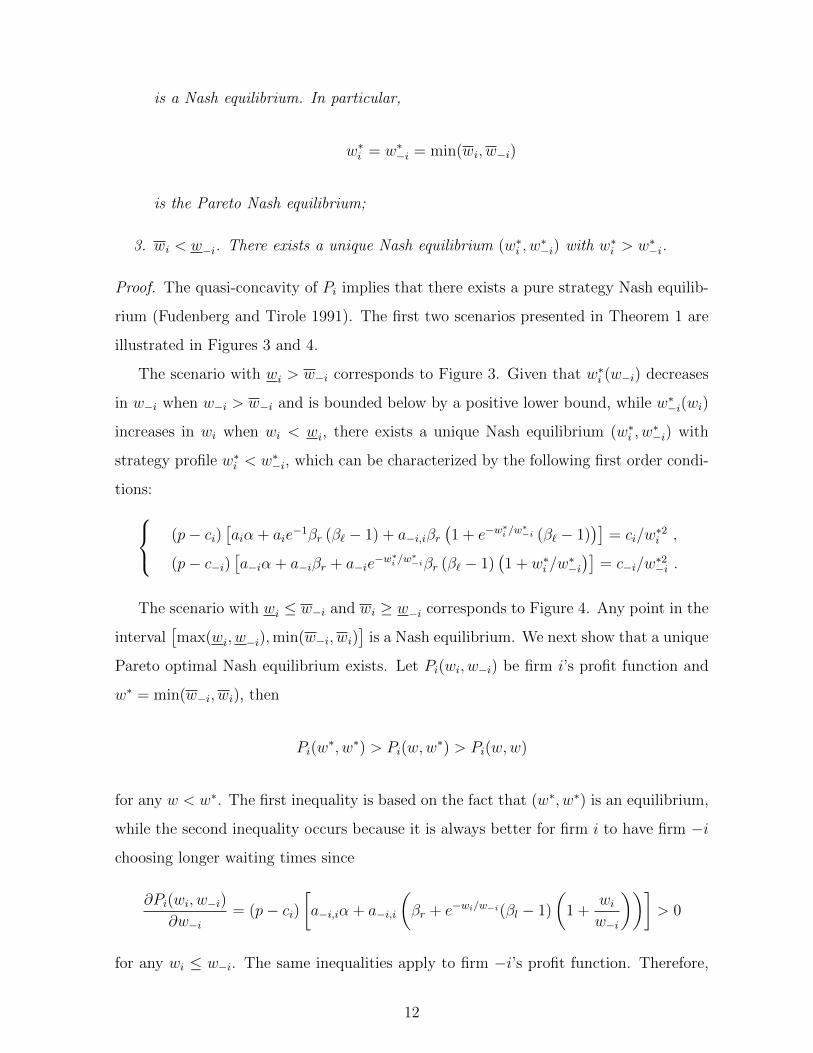
The scenario with wi ≤ w−i and wi ≥ w−i corresponds to Figure 4. Any point in the

interval[max(wi, w−i),min(w−i, wi)

]is a Nash equilibrium. We next show that a unique

Pareto optimal Nash equilibrium exists. Let Pi(wi, w−i) be firm i’s profit function and

w∗ = min(w−i, wi), then

Pi(w∗, w∗) > Pi(w,w

∗) > Pi(w,w)

for any w < w∗. The first inequality is based on the fact that (w∗, w∗) is an equilibrium,

while the second inequality occurs because it is always better for firm i to have firm −i

choosing longer waiting times since

∂Pi(wi, w−i)

∂w−i= (p− ci)

[a−i,iα + a−i,i

(βr + e−wi/w−i(βl − 1)

(1 +

wiw−i

))]> 0

for any wi ≤ w−i. The same inequalities apply to firm −i’s profit function. Therefore,

12

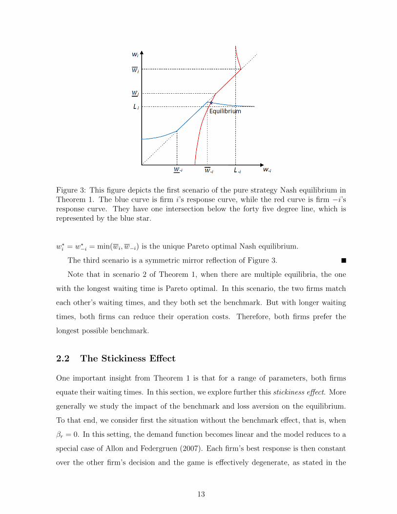
Figure 3: This figure depicts the first scenario of the pure strategy Nash equilibrium inTheorem 1. The blue curve is firm i’s response curve, while the red curve is firm −i’sresponse curve. They have one intersection below the forty five degree line, which isrepresented by the blue star.

w∗i = w∗−i = min(wi, w−i) is the unique Pareto optimal Nash equilibrium.

The third scenario is a symmetric mirror reflection of Figure 3.

Note that in scenario 2 of Theorem 1, when there are multiple equilibria, the one

with the longest waiting time is Pareto optimal. In this scenario, the two firms match

each other’s waiting times, and they both set the benchmark. But with longer waiting

times, both firms can reduce their operation costs. Therefore, both firms prefer the

longest possible benchmark.

2.2 The Stickiness Effect

One important insight from Theorem 1 is that for a range of parameters, both firms

equate their waiting times. In this section, we explore further this stickiness effect. More

generally we study the impact of the benchmark and loss aversion on the equilibrium.

To that end, we consider first the situation without the benchmark effect, that is, when

βr = 0. In this setting, the demand function becomes linear and the model reduces to a

special case of Allon and Federgruen (2007). Each firm’s best response is then constant

over the other firm’s decision and the game is effectively degenerate, as stated in the

13

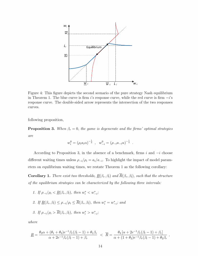
Figure 4: This figure depicts the second scenario of the pure strategy Nash equilibriumin Theorem 1. The blue curve is firm i’s response curve, while the red curve is firm −i’sresponse curve. The double-sided arrow represents the intersection of the two responsescurves.

following proposition,

Proposition 3. When βr = 0, the game is degenerate and the firms’ optimal strategies

are

w0i = (ρiaiα)−

12 , w0

−i = (ρ−ia−iα)−12 .

According to Proposition 3, in the absence of a benchmark, firms i and −i choose

different waiting times unless ρ−i/ρi = ai/a−i. To highlight the impact of model param-

eters on equilibrium waiting times, we restate Theorem 1 as the following corollary:

Corollary 1. There exist two thresholds, R(βr, βl) and R(βr, βl), such that the structure

of the equilibrium strategies can be characterized by the following three intervals:

1. If ρ−i/ρi < R(βr, βl), then w∗i < w∗−i;

2. If R(βr, βl) ≤ ρ−i/ρi ≤ R(βr, βl), then w∗i = w∗−i; and

3. If ρ−i/ρi > R(βr, βl), then w∗i > w∗−i;

where

R =θ3α + (θ1 + θ3)e

−1βr(βl − 1) + θ1βrα + 2e−1βr(βl − 1) + βr

< R =θ3 [α + 2e−1βr(βl − 1) + βr]

α + (1 + θ2)e−1βr(βl − 1) + θ2βr,

14

and

θ1 = a−i,i/a−i , θ2 = ai,−i/a−i < θ3 = ai/a−i . (2)

The complete derivation from Theorem 1 is in Appendix C. Corollary 1 shows that,

with the benchmark effect, the two firms will match each other’s waiting time at the

equilibrium as long as their profit margin ratio is within a certain range. We call this

phenomenon the stickiness effect. It is similar to the “focal price equilibrium” in a

different setting involving price competition with reference effect, as shown in Heidhues

and Koszegi (2008). We denote[R,R

]as the stickiness interval. The following result

determines the impact of the benchmark effect βr and the loss aversion effect βl on the

stickiness interval.

Proposition 4. R(βr, βl) and R(βr, βl) have the following structural properties:

1. When βr = 0, R = θ3 = R; when βr > 0, R < θ3 < R;

2. For fixed βl, R is decreasing in βr; R is increasing in βr;

3. For fixed βr,

– If βr < α, R is decreasing in βl; R is increasing in βl;

– If βr = α, R = (θ1 + θ3)/2 and R = 2θ3/(1 + θ2), which does not change with

βl;

– If βr > α, R is increasing in βl; R is decreasing in βl.

Proof. See Appendix D

Proposition 4 essentially states that the stickiness interval expands with βr, but may

either expand or shrink with βl depending on the relative strength of the benchmark

effect (βr) compared to the direct impact of waiting time (α).

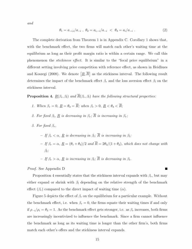
Figure 5 depicts the effect of βr on the equilibrium for a particular example. Without

the benchmark effect, i.e. when βr = 0, the firms equate their waiting times if and only

if ρ−i/ρi = θ3 = 1. As the benchmark effect gets stronger, i.e. as βr increases, both firms

are increasingly incentivized to influence the benchmark. Since a firm cannot influence

the benchmark as long as its waiting time is longer than the other firm’s, both firms

match each other’s offers and the stickiness interval expands.

15

0 2 4 6 8 100

0.5

1

1.5

2

2.5

3

βr

ρ −i/ρ

i

w*i < w*

−i

w*i = w*

−i

w*i > w*

−i

Figure 5: This figure depicts the combinations of ρ−i/ρi and βr such that w∗i > w∗−i,w∗i = w∗−i and w∗i < w∗−i. The upper curve denotes how R changes with βr, while thelower curve denotes how R changes with βr (ai = a−i = 1, a−i,i = ai,−i = 0.2, α = 1, βl =2).

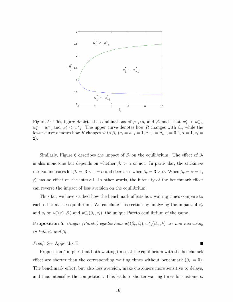
Similarly, Figure 6 describes the impact of βl on the equilibrium. The effect of βl

is also monotone but depends on whether βr > α or not. In particular, the stickiness

interval increases for βr = .3 < 1 = α and decreases when βr = 3 > α. When βr = α = 1,

βl has no effect on the interval. In other words, the intensity of the benchmark effect

can reverse the impact of loss aversion on the equilibrium.

Thus far, we have studied how the benchmark affects how waiting times compare to

each other at the equilibrium. We conclude this section by analyzing the impact of βr

and βl on w∗i (βr, βl) and w∗−i(βr, βl), the unique Pareto equilibrium of the game.

Proposition 5. Unique (Pareto) equilibriums w∗i (βr, βl), w∗−i(βr, βl) are non-increasing

in both βr and βl.

Proof. See Appendix E.

Proposition 5 implies that both waiting times at the equilibrium with the benchmark

effect are shorter than the corresponding waiting times without benchmark (βr = 0).

The benchmark effect, but also loss aversion, make customers more sensitive to delays,

and thus intensifies the competition. This leads to shorter waiting times for customers.

16

2 4 6 80

0.5

1

1.5

2

2.5

βl

ρ −i/ρ

i

βr = 0.3

2 4 6 80

0.5

1

1.5

2

2.5

βl

ρ −i/ρ

i

βr = 1

2 4 6 80

0.5

1

1.5

2

2.5

βl

ρ −i/ρ

i

βr = 3

wi* > w

−i*

wi* > w

−i*

wi* > w

−i*

wi* = w

−i*

wi* < w

−i*

wi* = w

−i*

wi* < w

−i*

wi* = w

−i*

wi* < w

−i*

Figure 6: This figure depicts the combinations of ρ−i/ρi and βl such that w∗i > w∗−i, w∗i =

w∗−i and w∗i < w∗−i, when βr = 0.3, 1 and 3. In each figure, the upper curve denotes theR function, while the lower curve denotes the R (ai = a−i = 1, a−i,i = ai,−i = 0.2, α = 1).

17

3 Average Benchmark and Reversal Effect

In this section we study the case where r = (wi + w−i)/2, which corresponds to the

so-called “product type norm” (Cadotte et al. 1987). We follow the approach of the

previous section, first characterizing the equilibrium of the game and then studying the

impact of the benchmark and loss aversion on the equilibrium.

3.1 Nash Equilibrium

We start by showing that firm i’s profit Pi is still a quasi-concave function in the average

benchmark case.

Proposition 6. Firm i’s profit Pi is a quasi-concave function of the waiting time wi.

Proof. See Appendix F

Given the quasi-concavity of Pi, we can study firm i’s best response curve w∗i as

a function of w−i. Proposition 6 implies that the first-order condition is sufficient to

determine firm i’s best response. Since firm i’s demand function λi is now everywhere

differentiable, we can define the derivative of λi with respect to wi at wi = w−i as

δi ≡ −∂λi∂wi

∣∣∣∣wi=w−i

= aiα +ai + a−i,i

2βr +

3ai + a−i,i2

e−1(βl − 1)βr ,

which leads to the following characterization of the response curve:

Proposition 7. Firm i’s best response curve, w∗i (w−i), is a piecewise function on the

following three intervals:

1. When w−i ∈ [0, w−i), we have w∗i > w−i and w∗i is quasi-convex in w−i;

2. When w−i = w−i, we have w∗i = w−i; and

3. When w−i ∈ (w−i,∞), we have w∗i < w−i and w∗i is quasi-concave in w−i,

where w−i =(ρiδi

)−1/2.

Proof. See Appendix G

18

Proposition 7 is very similar to Proposition 2 for the minimum benchmark case.

Specifically, when firm −i chooses a short waiting time (w−i < w−i), it is too costly for

firm i to match this delay. Thus firm i sets a waiting time w∗i longer than w−i. On the

other hand, when firm −i’s waiting time is not too short (w−i > w−i), it does not cost

much for firm i to set a higher benchmark. So firm i will choose a waiting time shorter

than w−i.

On the other hand, Proposition 7 differs from Proposition 2, which states that for the

minimum benchmark case when w−i is within a certain range, firm i’s optimal waiting

time w∗i equals w−i. According to Proposition 7, w∗i = w−i only when w−i = w−i. This

is because in the average form case, both firms can always influence the benchmark. By

contrast, in the minimum case, the firm with the longer waiting time has no impact on

the benchmark.

Following Proposition 7, we now provide the characterization of a pure strategy Nash

equilibrium, the existence of which is guaranteed by Proposition 6.

Theorem 2. A pure strategy Nash Equilibrium (w∗i , w∗−i) exists. Furthermore,

1. If wi > w−i, then w∗i < w∗−i.

2. If wi < w−i, then w∗i > w∗−i.

3. If wi = w−i, then w∗i = w∗−i.

Proof. See Appendix H

Note that the structure described by Theorem 2 is similar to the minimum benchmark

case. Although we are not able to prove the uniqueness of the pure strategy Nash

Equilibrium analytically, numerical tests in Appendix I show that under all the 625

choices of parameter settings, the equilibrium is unique. Our numerical study shows

further that both waiting times at the equilibrium decrease with parameters βr and βl,

which is also consistent with our findings for the minimum benchmark case.

3.2 The Reversal Effect

In this section we study the impact of the benchmark effect on the equilibrium. To

that end, we present the following Corollary from Theorem 2, which shows that the

19

equilibrium is characterized by a threshold on ρ−i/ρi.

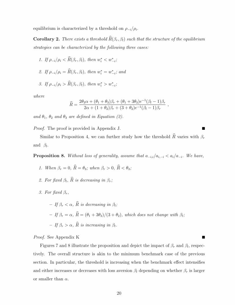
Corollary 2. There exists a threshold R(βr, βl) such that the structure of the equilibrium

strategies can be characterized by the following three cases:

1. If ρ−i/ρi < R(βr, βl), then w∗i < w∗−i;

2. If ρ−i/ρi = R(βr, βl), then w∗i = w∗−i; and

3. If ρ−i/ρi > R(βr, βl), then w∗i > w∗−i;

where

R =2θ3α + (θ1 + θ3)βr + (θ1 + 3θ3)e

−1(βl − 1)βr2α + (1 + θ2)βr + (3 + θ2)e−1(βl − 1)βr

,

and θ1, θ2 and θ3 are defined in Equation (2).

Proof. The proof is provided in Appendix J.

Similar to Proposition 4, we can further study how the threshold R varies with βr

and βl.

Proposition 8. Without loss of generality, assume that a−i,i/ai,−i < ai/a−i. We have,

1. When βr = 0, R = θ3; when βr > 0, R < θ3;

2. For fixed βl, R is decreasing in βr;

3. For fixed βr,

– If βr < α, R is decreasing in βl;

– If βr = α, R = (θ1 + 3θ3)/(3 + θ2), which does not change with βl;

– If βr > α, R is increasing in βl.

Proof. See Appendix K

Figures 7 and 8 illustrate the proposition and depict the impact of βr and βl, respec-

tively. The overall structure is akin to the minimum benchmark case of the previous

section. In particular, the threshold is increasing when the benchmark effect intensifies

and either increases or decreases with loss aversion βl depending on whether βr is larger

or smaller than α.

20

The previous analysis reveals that a market leader in terms of offering shorter waiting

time without the benchmark effect can sometimes become the follower (offering longer

waiting time) when the benchmark effect is strong enough. More specifically, when

βr = 0, the firms’ equilibrium strategies are equal to w0i and w0

−i from Proposition 3.

Assume, for instance, that firm i is the leader such that w0i < w0

−i. Following Corollary 2,

firm i becomes the follower with w∗i > w∗−i if ρ−i/ρi > R(βr, βl). Figure 7 illustrates this

reversal effect: When ρ−i/ρi is equal to 0.9, we have w∗i = w0i < w∗−i = w0

−i for βr = 0

(circle); but when the benchmark effect is strong enough (βr > 2 for instance), the order

is reversed with w∗−i < w∗i (star). We conclude this section by providing necessary and

sufficient conditions for this reversal effect to occur, as stated by the following result

which is a direct consequence of Corollary 2 and Proposition 8:

Proposition 9. Without loss of generality, assume that a−i,i/ai,−i < ai/a−i. There exist

values of βr and βl such that the leader of the duopoly without benchmark effect becomes

the follower with benchmark effect if and only if

θ1 + θ31 + θ2

<ρ−iρi

< θ3.

Thus, according to the proposition, the reversal can only occur when the ratio of

profit margins is within a certain range. The phenomena never occurs otherwise.

4 Conclusions

Empirical studies from both the Marketing and Decision Making literatures suggest

that customers can be influenced by the gap between their expected delays and a market

benchmark. We posit that this, in turn, should influence the way firms compete. The key

feature of our approach is that the benchmark is endogenous. This means that companies

can affect demand directly through their choices of waiting times, and indirectly by

manipulating the benchmark and making the competitor’s offer look worse.

Using an analytical approach, our study reveals several new findings. First the

presence of a benchmark decreases waiting times at the equilibrium. Second, depending

on how the benchmark is formed, either a stickiness or a reversal effect can occur. We

21

0 2 4 6 8 100.5

1

1.5

βr

ρ −i/ρ

i

wi* > w

−i*

wi* < w

−i*

Figure 7: This figure depicts the combinations of ρ−i/ρi and βr such that w∗i > w∗−iand w∗i < w∗−i. The decreasing curve denotes the function R (ai = a−i = 1, a−i,i =0.1, ai,−i = 0.5, α = 1, βl = 2).

have also disentangled the impacts that loss aversion and the benchmark effect have on

the equilibrium. We show in particular that in both cases, the direction of the impact

of loss aversion changes with the strength of the benchmark effect.

Our paper appears to be the first to study benchmark effects between service firms

competing on waiting times. Interesting extensions include investigating other forms

of benchmark, for example, the weighted average form. The equilibrium structure of

the weighted average form will be similar to the average case, and the reversal effect

result may hold as well. One can also generalize our model to other queuing systems.

Taking the M/G/1 queue, for example, the customers’ aggregate satisfaction with one

firm’s service will depend not only on the waiting time expectation, but also the higher

moments (e.g. variance), which will remarkably complicate the model and the analysis.

We could also consider the segmentation of customers with respect to their degree of

benchmark dependence and loss aversion or the presence of more than two firms. Equi-

librium may not be unique any more for these extensions. However, we suspect that

effects akin to the stickiness or reverse effects we identify in this paper should continue

to exist.

22

2 4 6 80.8

0.85

0.9

0.95

1

βl

ρ −i/ρ

i

βr=0.3

2 4 6 80.8

0.85

0.9

0.95

1

βl

ρ −i/ρ

i

βr=1

2 4 6 80.8

0.85

0.9

0.95

1

βl

ρ −i/ρ

i

βr=3

wi* > w

−i*

wi* > w

−i*

wi* > w

−i*

wi* < w

−i*

wi* < w

−i*

wi* < w

−i*

Figure 8: This figure depicts the combinations of ρ−i/ρi and βl such that w∗i > w∗−i and

w∗i < w∗−i, when βr = 0.3, 1 and 3. The curve in each figure denotes the function R(ai = a−i = 1, a−i,i = 0.1, ai,−i = 0.5, α = 1).

23

References

Allon, G. and Federgruen, A. (2007). Competition in service industries. Operations Research,

55(1):37–55.

Anderson, E. W. and Sullivan, M. W. (1993). The antecedents and consequences of customer

satisfaction for firms. Marketing Science, 12(2):125–143.

Blinder, A. S., Canetti, E. R., and Lebow, D. E. (1998). Asking About Prices: A New Approach

to Understanding Pricing Stickiness. Russell Sage Foundation, New York.

Cachon, G. P. and Harker, P. T. (2002). Competition and outsourcing with scale economies.

Management Science, 48(10):1314–1333.

Cadotte, E. R., Woodruff, R. B., and Jenkins, R. L. (1987). Expectations and norms in models

of consumer satisfaction. Journal of Marketing Research, 24(3):305–314.

Crouzeix, J. P. (1980). On second order conditions for quasiconvexity. Mathematical Program-

ming, 18:349–352.

De Vany, A. S. and Saving, T. R. (1983). The economics of quality. Journal of Political

Economy, 91(6):979–1000.

Erdem, T., Mayhew, G., and Sun, B. (2001). Understanding reference-price shoppers: A

within- and cross- category analysis. Journal of Marketing Research, 38(4):445–457.

Fudenberg, D. and Tirole, J. (1991). Game Theory. MIT Press.

Gaur, V. and Park, Y. H. (2007). Asymmetric consumer learning and inventory competition.

Management Science, 53(2):227–240.

Hall, J. and Porteus, E. (2000). Customer service competition in capacitated systems. Manu-

facturing and Service Operations Management, 2(2):144–165.

Hassin, R. and Haviv, M. (2002). To Queue or Not to Queue: Equilibrium Behavior in Queue-

ing Systems. Springer.

Heidhues, P. and Koszegi, B. (2008). Competition and price variation when consumers are loss

averse. American Economic Review, 98(4):1245C1268.

Helson, H. (1964). Adaptation-Level Theory. Harper and Row, New York.

Ho, T. H. and Zheng, Y. S. (2004). Setting customer expectation in service delivery: An

integrated marketing-operations perspective. Management Science, 50(4):479–488.

Kahneman, D. and Tversky, A. (1979). Prospect theory: An analysis of decision under risk.

Econometrica, 47(2):263–292.

24

Kalai, E., Kamien, M. I., and Rubinovitch, M. (1992). Optimal service speeds in a competitive

environment. Management Science, 38(8):1154–1163.

Leclerc, F., Schmitt, B. H., and L., D. (1995). Waiting time and decision making: Is time like

money? Journal of Consumer Research, 22(1):110–119.

Lin, J. H., Lee, T. R., and Jen, W. (2008). Assessing asymmetric response effect of behavioral

intention to service quality in an integrated psychological decision-making process model

of intercity bus passengers: A case of taiwan. Transportation, 35:129–144.

Liu, B. S., Petruzzi, N. C., and Sudharshan, D. (2007). A service effort allocation model for

assessing customer lifetime value in service marketing. Journal of Services Marketing,

21(1):24–35.

Niedrich, R. W., Sharma, S., and Wedell, D. (2001). Reference price and price perceptions: A

comparison of alternative models. Journal of Consumer Research, 28(3):339–354.

Popescu, I. and Wu, Y. (2007). Dynamic pricing strategies with reference effects. Operations

Research, 55(3):413–429.

So, K. C. (2000). Price and time competition for service delivery. Manufacturing and Service

Operations Management, 2(4):392–409.

Wedell, D. H. (1995). Contrast effects in paired comparisons: Evidence for both stimulus-based

and response-based processes. Journal of Experimental Psychology: Human Perception

and Performance, 21(5):1158–1173.

Zeithaml, V. A., Berry, L. L., and Parasuraman, A. (1993). The nature and determinants of

customer expectations of service. Journal of the Academy of Marketing Science, 21(1):1–

12.

Zhou, J. (2011). Reference dependence and market competition. Journal of Economics and

Management Strategy, 20(4):1073–1097.

25

A Proof of Proposition 1

Proof. We first prove that Pi is a quasi-concave function of wi. We first show that firm

i’s profit function Pi(wi, w−i) is concave in wi when wi ≥ w−i. When wi ≥ w−i, r = w−i

and

Pi(wi, w−i) = (p− ci) [a0 + aiSi(wi, w−i)− a−i,iS−i(w−i, w−i)]−ciwi

,

where

Si(wi, w−i) = −αwi + βr

[(w−i − wi)− e−

w−iwi (β` − 1)wi

]and

S−i(w−i, w−i) = −αw−i − βre−1 (β` − 1)w−i.

Take the first and second order derivatives of Pi with respect to wi:

∂Pi∂wi

= −(p− ci)ai{α + βr

[1 + e

−w−iwi (β` − 1)

(1 +

w−iwi

)]}+

ciw2i

∂2Pi∂w2

i

= −(p− ci)aiβre−w−iwi (β` − 1)

w2−i

w3i

− 2ciw3i

< 0 .

Therefore Pi is concave in wi when wi ≥ w−i.

We next show that Pi is quasi-concave in wi when wi ≤ w−i. When wi ≤ w−i, r = wi

and

Pi(wi, w−i) = (p− ci) [a0 + aiSi(wi, wi)− a−i,iS−i(w−i, wi)]−ciwi

,

where

Si(wi, wi) = −αwi − βre−1 (β` − 1)wi

and

S−i(w−i, wi) = −αw−i + βr

[(wi − w−i)− e

− wiw−i (β` − 1)w−i

].

For simplicity, we let P (wi) = Pi(wi, w−i). By definition, given any w1 < w2 < w3 ≤ w−i,

P (wi) is quasi-concave in wi iff P (w2) ≥ min{P (w1), P (w3)}.

First, assume that P (w1) ≤ P (w3), we then prove P (w2) ≥ P (w1). Let A = aiα +

26

aiβre−1 (β` − 1) + a−i,iβr and B = a−i,iβr (β` − 1)w−i, we have A,B > 0, then

P (w3)− P (w1) = (p− ci)[A(w1 − w3) +B

(e− w3w−i − e−

w1w−i

)]− ci

w1 − w3

w1w3

≥ 0 .

Therefore,P (w3)− P (w1)

w1 − w3

w3 = (p− ci) [Aw3 +Bg(w3)]−ciw1

≤ 0 ,

where g(w3) = e− w3w−i −e

− w1w−i

w1−w3w3. Since

∂g

∂w3

=e− w3w−i

(w1 + w3

w−i(w3 − w1)

)− e−

w1w−iw1

(w1 − w3)2> 0 ,

we have g(w2) < g(w3). Therefore,

P (w2)− P (w1)

w1 − w2

w2 = (p− ci) [Aw2 +Bg(w2)]−ciw1

< (p− ci) [Aw3 +Bg(w3)]−ciw1

=P (w3)− P (w1)

w1 − w3

w3 ≤ 0 .

Given that w1 < w2, we have P (w2) > P (w1).

Assume that P (w1) ≥ P (w3); we then prove P (w2) ≥ P (w3). Using the same

method, we have:

P (w1)− P (w3)

w3 − w1

w1 = (p− ci) [Aw1 +Bh(w1)]−ciw3

≥ 0 ,

where h(w1) = e− w1w−i −e

− w3w−i

w3−w1w1. Since

∂h

∂w1

=e− w1w−i

(w3 − w1

w−i(w3 − w1)

)− e−

w3w−iw3

(w3 − w1)2> 0 ,

27

we have h(w2) > h(w1). Therefore,

P (w2)− P (w3)

w3 − w2

w2 = (p− ci) [Aw2 +Bh(w2)]−ciw3

> (p− ci) [Aw1 +Bh(w1)]−ciw3

=P (w1)− P (w3)

w3 − w1

w1 ≥ 0 .

Given that w3 > w2, we have P (w2) > P (w3). It follows that

P (w2) > min{P (w1), P (w3)}.

Given that firm i’s profit function Pi(wi, w−i) is concave in wi when wi ≥ w−i and is

quasi-concave in wi when wi ≤ w−i, Pi can only be one of the four cases shown in Figure

1. To prove that Pi is quasi-concave in wi, we need only rule out case (4). Assuming

that

∂Pi∂wi

∣∣∣∣wi↑w−i

= −(p− ci)[aiα + a−i,iβr + (ai + a−i,i)βre

−1 (β` − 1)]

+ciw2−i

< 0 ,

then we have

∂Pi∂wi

∣∣∣∣wi↓w−i

= −(p− ci)[aiα + aiβr + 2aiβre

−1 (β` − 1)]

+ciw2−i

< −(p− ci)[aiα + a−i,iβr + (ai + a−i,i)βre

−1 (β` − 1)]

+ciw2−i

=∂Pi∂wi

∣∣∣∣wi↑w−i

< 0 .

So if the derivative of Pi with respect to wi is negative on the left of w−i, it can not be

positive on the right of w−i. Case (4) in Figure 1 is not possible. The result holds.

We next show that Pi is supermodular when wi > w−i, and submodular when wi <

w−i. When wi > w−i,

∂Pi∂wi

∣∣∣∣wi>w−i

= −(p− ci)[aiα + aiβr + aiβre

−w−iwi (β` − 1)

(1 +

w−iwi

)]+

ciw2i

,

28

so∂2Pi

∂wi∂w−i

∣∣∣∣wi>w−i

= (p− ci)aiβr(βl − 1)e−w−i

wiw−iw2i

.

Therefore, Pi is supermodular when wi > w−i.

When wi < w−i,

∂Pi∂wi

∣∣∣∣wi<w−i

= −(p− ci)[aiα + aiβre

−1 (β` − 1) + a−i,iβr

(1 + e

− wiw−i (β` − 1)

)]+

ciw2i

,

so∂2Pi

∂wi∂w−i

∣∣∣∣wi<w−i

= −(p− ci)a−i,iβr(βl − 1)e− wiw−i

wiw2−i.

Therefore, Pi is submodular when wi < w−i.

B Proof of Proposition 2

Proof. The quasi-concavity of Pi implies that for any given w−i, the first-order condition

is a sufficient condition for firm i’s best response. Pi can be any of the three cases (1, 2,

3) as shown in Figure 1.

If ∂Pi/∂wi|wi↓w−i> 0, then it corresponds to case (1). Since

∂Pi∂wi

∣∣∣∣wi↓w−i

= −(p− ci)[aiα + aiβr + 2aiβre

−1 (β` − 1)]

+ciw2−i,

∂Pi/∂wi|wi↓w−i> 0 is equivalent to w−i <

(ρiδi)−1/2

. In this case, w∗i will be on the right

of w−i. Since Pi is supermodular when wi > w−i, firm i’s best response w∗i is increasing

in w−i in this scenario.

If ∂Pi/∂wi|wi↑w−i≥ 0 and ∂Pi/∂wi|wi↓w−i

≤ 0, which is equivalent to(ρiδi)−1/2 ≤

w−i ≤ (ρiδi)−1/2, it corresponds to case (2). In this case, w∗i = w−i.

If ∂Pi/∂wi|wi↑w−i< 0, then it corresponds to case (3). Since

∂Pi∂wi

∣∣∣∣wi↑w−i

= −(p− ci)[aiα + a−i,iβr + (ai + a−i,i)βre

−1 (β` − 1)]

+ciw2−i,

29

∂Pi/∂wi|wi↑w−i< 0 is equivalent to w−i > (ρiδi)

−1/2. In this case, w∗i will be on the

left of w−i. Given that Pi is submodular when wi < w−i, we have firm i’s best re-

sponse w∗i decreasing in w−i in this scenario. Therefore, w∗i ≥ w∗i (∞) = Li where

Li = (ρi [aiα + aie−1βr (β` − 1) + a−i,iβrβ`])

−1/2.

C Proof of Corollary 1

Proof. According to Theorem 1, if wi > w−i, then the equilibrium strategies w∗i < w∗−i.

The condition corresponds to

wiw−i

=

(ρ−iρi· α + 2e−1βr(βl − 1) + βrθ3α + (θ1 + θ3)e−1βr(βl − 1) + θ1βr

)− 12

> 1 ,

which leads to ρ−i/ρi < R, where

R =θ3α + (θ1 + θ3)e

−1βr(βl − 1) + θ1βrα + 2e−1βr(βl − 1) + βr

.

If wi ≤ w−i and wi ≥ w−i, then the equilibrium strategies w∗i = w∗−i. The condition

corresponds to ρ−i/ρi ≥ R and

wiw−i

=

(ρ−iρi· α + (1 + θ2)e

−1βr(βl − 1) + θ2βrθ3 [α + 2e−1βr(βl − 1) + βr]

)− 12

≥ 1 ,

which is equivalent to R ≤ ρ−i/ρi ≤ R, where

R =θ3 [α + 2e−1βr(βl − 1) + βr]

α + (1 + θ2)e−1βr(βl − 1) + θ2βr.

If wi < w−i, then the equilibrium strategies w∗i > w∗−i. The condition corresponds to

ρ−i/ρi > R.

D Proof of Proposition 4

When we fix βl, since θ3 > (θ1 + θ3)/2 and θ3 > θ1, we have R decreasing in βr and

bounded from below by [(θ1 + θ3)e−1(βl − 1) + θ1] / [2e−1(βl − 1) + 1]. On the other

30

hand, since θ3 < 2θ3/(1 + θ2) and θ3 < θ3/θ2, we have R increasing in βr and bounded

from above by [2θ3e−1(βl − 1) + θ3] / [(1 + θ2)e

−1(βl − 1) + θ2].

When we fix βr, to analyze R, we need to compare A = (θ3α + θ1βr)/(α + βr) and

B = (θ1 + θ3)/2. If βr < α, we have A > B, so R is decreasing in βl and bounded from

below by B; if βr = α, we have A = B, so R = B; if βr > α, we have A < B, so R is

increasing in βl and bounded from above by B.

To analyze R, we need to compare C = (θ3α+θ3βr)/(α+θ2βr) and D = 2θ3/(1+θ2).

If βr < α, we have C < D, so R is increasing in βl and bounded from above by D; if

βr = α, we have C = D, so R2 = D; if βr > α, we have C > D, so R is decreasing in βl

and bounded from below by D.

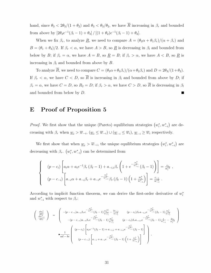
E Proof of Proposition 5

Proof. We first show that the unique (Pareto) equilibrium strategies(w∗i , w

∗−i)

are de-

creasing with βr when wi > w−i, (wi ≤ w−i) ∪ (w−i ≤ wi), w−i ≥ wi respectively.

We first show that when wi > w−i, the unique equilibrium strategies(w∗i , w

∗−i)

are

decreasing with βr.(w∗i , w

∗−i)

can be determined from

(p− ci)

[aiα + aie

−1βr (β` − 1) + a−i,iβr

(1 + e

− w∗i

w∗−i (β` − 1)

)]= ci

w∗2i,

(p− c−i)

[a−iα + a−iβr + a−ie

− w∗i

w∗−i βr (β` − 1)

(1 +

w∗i

w∗−i

)]= c−i

w∗2−i.

According to implicit function theorem, we can derive the first-order derivative of w∗iand w∗−i with respect to βr:

dw∗i

dβrdw∗

−i

dβr

=

−(p− c−i)a−iβre−

w∗i

w∗−i (β` − 1)

w∗2i

w∗3−i

− 2c−i

w∗3−i

(p− ci)βra−i,ie−

w∗i

w∗−i (β` − 1)

w∗i

w∗2−i

−(p− c−i)a−iβre−

w∗i

w∗−i (β` − 1)

w∗i

w∗2−i

(p− ci)βra−i,ie−

w∗i

w∗−i (β` − 1) 1

w∗−i− 2ciw∗3

i

•1

ad− bc

(p− ci)

aie−1(β` − 1) + a−i,i + a−i,ie−

w∗i

w∗−i (β` − 1)

(p− c−i)

a−i + a−ie−

w∗i

w∗−i (β` − 1)

(1 +

w∗i

w∗−i

)

,

31

where

ad− bc > (p− ci)(p− c−i)a−iβra−i,ie− w∗

iw∗−i (β` − 1)(a−iα + βr)

2

w∗−i

(2

w∗i− 1

w∗−i

)> 0

since w∗i < w∗−i. So we have

dw∗i

dβr< −

(p− ci)(p− c−i)(ad− bc)w∗

−iaiβra−i,ie

−w∗

iw∗

−i (β` − 1)

1 + e−

w∗i

w∗−i (β` − 1)

(1 +

w∗i

w∗−i

)(2−w∗i

w∗−i

)< 0

and

dw∗−i

dβr< −

(p− ci)(p− c−i)(ad− bc)w∗

i

a−iβra−i,ie−

w∗i

w∗−i (β` − 1)

1 + e−

w∗i

w∗−i (β` − 1)

(1 +

w∗i

w∗−i

)(2−w∗i

w∗−i

)< 0 .

Therefore the result holds for wi > w−i.

When w−i ≥ wi, we can show that the unique equilibrium strategies (w∗i , w∗−i) de-

crease with βr using the same method as in the last scenario.

When wi ≤ w−i and w−i ≤ wi, the Pareto optimal equilibrium strategies w∗i = w∗−i =

min(wi, w−i) decrease with βr since both wi and w−i decrease with βr.

Therefore, the unique (Pareto) equilibrium waiting times decrease with βr.

We next show that the unique (Pareto) equilibrium strategies (w∗i , w∗−i) are decreasing

with βl when wi > w−i, (wi ≤ w−i) ∪(w−i ≤ wi

), w−i ≥ wi, respectively.

We first show that when wi > w−i, the unique equilibrium strategies are decreasing

with βl. (w∗i , w∗−i) can be determined from

(p− ci)

[aiα + aie

−1βr (β` − 1) + a−i,iβr

(1 + e

− w∗i

w∗−i (β` − 1)

)]= ci

w∗2i,

(p− c−i)

[a−iα + a−iβr + a−ie

− w∗i

w∗−i βr (β` − 1)

(1 +

w∗i

w∗−i

)]= c−i

w∗2−i.

According to implicit function theorem, we can derive the first-order derivative of w∗i

32

and w∗−i with respect to βl:

dw∗i

dβldw∗

−i

dβl

=

−(p− c−i)a−iβre−

w∗i

w∗−i (β` − 1)

w∗2i

w∗3−i

− 2c−i

w∗3−i

(p− ci)βra−i,ie−

w∗i

w∗−i (β` − 1)

w∗i

w∗2−i

−(p− c−i)a−iβre−

w∗i

w∗−i (β` − 1)

w∗i

w∗2−i

(p− ci)βra−i,ie−

w∗i

w∗−i (β` − 1) 1

w∗−i− 2ciw∗3

i

•1

ad− bc

(p− ci)βr

aie−1 + a−i,ie−

w∗i

w∗−i

(p− c−i)a−iβre

−w∗

iw∗

−i

(1 +

w∗i

w∗−i

) ,

where ad− bc > 0. Since w∗i < w∗−i, we have

dw∗idβl

< −(p− c−i)(p− ci)β2r

(ad− bc)w∗−ia−ia−i,ie

−2 w∗i

w∗−i (β` − 1)

(1 +

w∗iw∗−i

)(2− w∗i

w∗−i

)< 0

and

dw∗−idβl

< −(p− c−i)(p− ci)β2r

(ad− bc)w∗ia−ia−i,ie

−2 w∗i

w∗−i (β` − 1)

(1 +

w∗iw∗−i

)(2− w∗i

w∗−i

)< 0 .

Therefore the result holds for wi > w−i.

We can easily show that when (wi ≤ w−i) ∪(w−i ≤ wi

)or w−i ≥ wi, the unique

(Pareto) equilibrium strategies decrease with βl.

F Proof of Proposition 6

Proof. Firm i’s profit function is:

Pi(wi, w−i) = (p− ci) [a0 + aiSi(wi, r)− a−i,iS−i(w−i, r)]−ciwi

,

where

Si(wi, r) = −αwi + βr

[wi + w−i

2− wi − e−

wi+w−i2wi (βl − 1)wi

].

If

∂Pi

∂wi= −(p− ci)

[aiα+

ai + a−i,i

2βr + aiβre

− rwi (βl − 1)

(1 +

w−i

2wi

)+ a−i,iβre

− rw−i (βl − 1)

1

2

]+

ci

w2i

= 0 ,

33

then

∂2Pi

∂w2i

= (p− ci)βr(βl − 1)1

4w−i

(−aie

− rwi

w3−iw3i

+ a−i,ie− r

w−i

)−

2ci

w3i

= −(p− ci)2

wi

{aiα+

ai + a−i,i

2βr + βr(βl − 1)

[aie

− rwi

(w2

−i8w2

i

+w−i

2wi+ 1

)+ a−i,ie

− rw−i

(1

2−

wi

8w−i

)]}

< −(p− ci)2

wi

{aiα+

ai + a−i,i

2βr + βr(βl − 1)a−i,i

[e− r

wi

(w2

−i8w2

i

+w−i

2wi+ 1

)+ e

− rw−i

(1

2−

wi

8w−i

)]}< 0 .

The second equality is supported by ∂Pi/∂wi = 0, while the last inequality is because

e−1+x2

(1 +

x

2+x2

8

)+ e−

1+x2x

(1

2− 1

8x

)> 0

for any x = w−i/wi ≥ 0.

According to the theorem in Crouzeix (1980), if function Pi is twice differentiable,

and if ∂Pi/∂wi = 0 implies ∂2Pi/∂w2i < 0, then Pi is a quasi-concave function of wi.

G Proof of Proposition 7

Proof. Since Pi is quasi-concave in wi and (∂Pi/∂wi)|wi=0 =∞ > 0 and

∂Pi∂wi

∣∣∣∣wi=∞

= −(p− ci)[aiα +

ai + a−i,i2

βr + aiβr(βl − 1)e−12

]< 0 ,

given firm −i’s waiting time standard w−i, firm i’s unique best response w∗i can bedetermined by the following equation:

∂Pi

∂wi= −(p− ci)

[aiα+

ai + a−i,i

2βr + aiβre

− rwi (βl − 1)

(1 +

w−i

2wi

)+ a−i,iβre

− rw−i (βl − 1)

1

2

]+

ci

w2i

= 0 .

We can infer that if (∂Pi/∂wi)|wi=w−i> 0, then w∗i is on the right of w−i and

w∗i > w−i. The condition is

∂Pi∂wi

∣∣∣∣wi=w−i

= −(p− ci)[aiα +

ai + a−i,i2

βr +3ai + a−i,i

2e−1(βl − 1)βr

]+

ciw2−i> 0 ,

which is equivalent to

w−i < w−i =(ρiδi

)− 12.

34

Similarly, if w−i = w−i, then (∂Pi/∂wi)|wi=w−i= 0, which means that w∗i = w−i;

while if w−i > w−i, then (∂Pi/∂wi)|wi=w−i< 0, which implies that w∗i is on the left of

w−i and w∗i < w−i.

We next analyze the structure of the best response curve w∗i (w−i). The first order

derivative of w∗i with respect to w−i is:

dw∗idw−i

=βr(βl − 1)

w∗2i

4w2−i

(aie− rw∗iw3

−iw∗3i− a−i,ie

− rw−i)

2aiα+ βr(ai + a−i,i) + βr(βl − 1)[aie− rw∗i

(2 + w−i

w∗i

+w2

−i4w∗2

i

)+ a−i,ie

− rw−i 3

4

] =A

B,

where A and B denote the numerator and the denominator respectively. Clearly, B > 0.

If dw∗i /dw−i = 0, which is equivalent to A = 0 and aie−r/w∗

iw3−i/w

∗3i = a−i,ie

−r/w−i ,

then

d2w∗i

dw2−i

= − A

B2

dB

dw−i− 2A

Bw∗iw−i

+βr(βl − 1)

w∗i

4w3−i

[aie

− rw∗

iw3

−i

w∗3i

(3− w−i

2w∗i

)− a−i,ie

− rw−i

w∗i

2w−i

]B

=βr(βl − 1)

w∗i

4w3−ia−i,ie

− rw−i

(3− w−i

2w∗i− w∗

i

2w−i

)B

.

Numerical tests show that 3−w−i/2w∗i −w∗i /2w−i > 0 if aie−r/w∗

iw3−i/w

∗3i = a−i,ie

−r/w−i

and w∗i > w−i; while 3− w−i/2w∗i − w∗i /2w−i < 0 if aie−r/w∗

iw3−i/w

∗3i = a−i,ie

−r/w−i and

w∗i < w−i. Therefore, when w∗i > w−i, if dw∗i /dw−i = 0, we have d2w∗i /dw2−i > 0; when

w∗i < w−i, if dw∗i /dw−i = 0, we have d2w∗i /dw2−i < 0. According to the theorem in

Crouzeix (1980), given that function w∗i (w−i) is twice differentiable, w∗i is quasi-convex

in w−i when w∗i > w−i and is quasi-concave in w−i when w∗i < w−i.

H Proof of Theorem 2

Proof. Since firm i’s profit Pi is quasi-concave in waiting time wi, there exists a pure

strategy Nash Equilibrium (Fudenberg and Tirole (1991)), which means that there are

intersections of the two best-response curves w∗i (w−i) and w∗−i(wi).

To prove scenario 1, we need only show that when wi > w−i, the intersections of the

two response curves are below the forty-five degree line in the (w−i, wi) space, which is

equivalent to no intersection above the forty-five degree line.

The best response curve w∗i (w−i) above the forty-five degree line can be denoted as

35

ci 1 2 3 4 5ai 0.6 0.8 1 1.2 2.1βr 1 4 7 10 13βl 2 4 6 8 10

Table 1: Model parameters.

(w−i, w∗i ) with w−i < w−i; while the best response curve w∗−i(wi) above the forty-five

degree line can be denoted as (w∗−i, wi) with wi > wi.

According to Proposition 7, w∗−i(wi) is quasi-concave in wi when wi > wi, so we have

w∗−i ≥ min(w∗−i(wi), w

∗−i(∞)

), where w∗−i(wi) = wi > w−i and

w∗−i(∞) =

c−i

(p− c−i)[a−iα +

a−i+ai,−i2

βr +ai,−i2e−

12 (βl − 1)βr

] 1

2

> wi > w−i .

Therefore, when wi > wi, we have w∗−i > w−i. As a result, the curve (w∗−i, wi) does not

intersect with the curve (w−i, w∗i ) where w−i < w−i. So there is no intersection of the

two response curves above the forty-five degree line when wi > w−i, which implies that

in the Nash Equilibrium, w∗i < w∗−i.

Scenarios 2 and 3 can be proved in the same way.

I Uniqueness of the Nash equilibrium when r = (wi+

w−i)/2

In this appendix we numerically study whether the pure strategy Nash equilibrium is

unique when r = (wi + w−i)/2. We conduct an extensive computational study with

varied model parameter as indicated in Table 1.

Specifically, we fix firm −i’s parameters and change firm i’s parameters according

to Table 1. While firm −i’s capacity cost, c−i, is assumed to be 3, we vary firm −i’s

capacity cost, ci, to be 1, 2, 3, 4 and 5. We set α = 2. Firm −i’s parameter a−i is set

to be 1, while firm i’s parameter ai is assumed to be 0.6, 0.8, 1, 1.2 or 2.1. In addition,

we vary the reference effect parameter, βr, to be 1, 4, 7, 10 and 13. The loss aversion

parameter, βl is assumed to be 2, 4, 6, 8 and 10. Finally, both a−i,i and ai,−i take the

36

value of 0.2. The above choices of parameters cover all three scenarios in Theorem 2

and all three scenarios in Proposition 2.

In total, we vary 4 model parameters. There are altogether 625 possible combinations

of model parameters. All the cases are such that the Nash equilibrium is unique.

J Proof of Corollary 2

Proof. From Theorem 2 we know that in order to determine the order of the two firms’

equilibrium strategies w∗i and w∗−i, we need only compare wi and w−i. If wi > w−i, then

the equilibrium strategies w∗i < w∗−i. The condition corresponds to

wiw−i

=

(ρ−iρi· 2α + (1 + θ2)βr + (3 + θ2)e

−1(βl − 1)βr2θ3α + (θ1 + θ3)βr + (θ1 + 3θ3)e−1(βl − 1)βr

)− 12

> 1 ,

which is equivalent to ρ−i/ρi < R, where

R =2θ3α + (θ1 + θ3)βr + (θ1 + 3θ3)e

−1(βl − 1)βr2α + (1 + θ2)βr + (3 + θ2)e−1(βl − 1)βr

.

If wi = w−i, then the equilibrium strategies w∗i = w∗−i. The condition corresponds to

ρ−i/ρi = R. If wi < w−i, then the equilibrium strategies w∗i > w∗−i. The condition

corresponds to ρ−i/ρi > R.

K Proof of Proposition 8

When we fix βl, to analyze R, we need to compare θ3 and

E =θ1 + θ3 + (θ1 + 3θ3)e

−1(βl − 1)

1 + θ2 + (3 + θ2)e−1(βl − 1).

Since a−i,i/ai,−i < ai/a−i, we have θ3 > E, hence R is decreasing in βr and bounded

from below by E.

37

When we fix βr, to analyze R, we need to compare

F =2θ3α + (θ1 + θ3)βr

2α + (1 + θ2)βr

and G = (θ1 + 3θ3)/(3 + θ2). If βr < α, we have F > G, so R is decreasing in βl and

bounded from below by G; if βr = α, we have F = G, so R = G; if βr > α, we have

F < G, so R is increasing in βl and bounded from above by G.

L Proof of Proposition 9

When βr = 0, we have R = θ3; when βr > 0, R stays below θ3 and is bounded from

below by (θ1 + θ3)/(1 + θ2), given that a−i,i/ai,−i < ai/a−i (θ1/θ2 < θ3). Therefore, as

long as ρ−i/ρi is within the interval of ((θ1 + θ3)/(1 + θ2), θ3), there always exist values

of βr and βl for the reversal effect to happen. On the other hand, if we observe the

reversal effect, then ρ−i/ρi is always within the interval.

38