Tilburg University When a Master Dies Penasse, Julien ...

Tilburg University

When a Master Dies

Penasse, Julien; Renneboog, Luc; Scheinkman, Jose

Publication date:2020

Document VersionEarly version, also known as pre-print

Link to publication in Tilburg University Research Portal

Citation for published version (APA):Penasse, J., Renneboog, L., & Scheinkman, J. (2020). When a Master Dies: Speculation and Asset Float.(CentER Discussion Paper; Vol. 2020-010). CentER, Center for Economic Research.

General rightsCopyright and moral rights for the publications made accessible in the public portal are retained by the authors and/or other copyright ownersand it is a condition of accessing publications that users recognise and abide by the legal requirements associated with these rights.

• Users may download and print one copy of any publication from the public portal for the purpose of private study or research. • You may not further distribute the material or use it for any profit-making activity or commercial gain • You may freely distribute the URL identifying the publication in the public portal

Take down policyIf you believe that this document breaches copyright please contact us providing details, and we will remove access to the work immediatelyand investigate your claim.

Download date: 02. Feb. 2022

https://research.tilburguniversity.edu/en/publications/33ff63e3-8842-44c7-92f5-6cb3e93370c0

No. 2020-010

WHEN A MASTER DIES: SPECULATION AND ASSET FLOAT

By

Julien Pénasse, Luc Renneboog, José A. Scheinkman

19 March 2020

ISSN 0924-7815 ISSN 2213-9532

When a Master Dies: Speculation and Asset Float∗

Julien Penasse† Luc Renneboog‡ Jose A. Scheinkman§

March 4, 2020

Abstract

The death of an artist constitutes a negative supply shock to his future produc-tion; in finance terms, this supply shock reduces the artist’s float. Intuition maythus suggest that this supply shock reduces the future auction volume of the artist.However, if collectors have fluctuating heterogeneous beliefs, since they cannot sellshort, prices overweigh optimists’ beliefs and have a speculative component. Ifcollectors have limited capacity to bear risk, an increase in float may decrease sub-sequent turnover and prices (Hong et al., 2006). Symmetrically, a negative supplyshock leads to an augmentation of prices and turnover. We find strong support forthis prediction in the data on art auctions that we examine.

∗We would like to thank Marcelo Fernandes, Ed Glaeser, Florian Heider, Harrison Hong, and seminarparticipants at Columbia University, at the Arrow Lecture at the Hebrew University of Jerusalem, SBFIN(Brazil), Tokyo University, University of Luxembourg, the European Winter Finance Conference, and theYale-RFS Real and Private-Value Assets Conference for comments, Jialin Yu for providing the originaldata of Xiong and Yu (2011), and John Silberman for a insightful conversation on artists’ estates. Wealso thank Raghav Bansal, Zoey Chopra, Kristine Fu, and Emilio Garcia for excellent research assistance.

†University of Luxembourg.‡Tilburg University.§Columbia University, Princeton University and NBER.

Pour moi les tableaux de grand prixSont ceux que plus cher on m’achete.

Apres tout, que m’importe le talent? 1

I. Introduction

Around 1660, an Italian art dealer brought bad news to Rembrandt: his style of painting

was no longer in vogue and sold at lower prices. Rembrandt did not yield to the art

dealer’s suggestion to start painting in the idealizing style of the classic painters, but

thought up a cunning plan. He disappeared and had the rumor spread that he had died

(De Wilt, 2006). As a consequence, works by a ‘dead’ Rembrandt were sold for up to

three times the normal price.2

This anecdote illustrates that the unexpected death of an artist leads to higher prices,

a natural consequence of the lower future supply relative to expectations. It is natural to

expect that the lower supply would also lead to a smaller volume of trade in the future

but theories of speculation based on fluctuating differences in beliefs and short-selling

restrictions (Harrison and Kreps, 1978; Scheinkman and Xiong, 2003) suggest that the

lower outstanding supply may actually lead to an increase in both prices and turnover

(Hong et al. 2006). A smaller float means that the marginal future buyer is likely to

have a more optimistic view, which makes the option to sell more valuable for the current

owner. When the marginal future buyer is more optimistic, it is also less probable that

a current owner’s valuation will stay among the highest in the future leading to a higher

1“For me, highly priced paintings are those that I can sell ever more expensively. After all, whyshould I care about talent?” Quote from Forbeck, the art-dealer in the play “Rembrandt ou la Venteapres deces” (by Charles-Guillaume Etienne, 1777-1845) (see Spieth 2017).

2Several versions of this anecdote circulate. The aforementioned play has been performed in Francesince 1800. According to the play, Rembrandt and his first wife Saskia van Uylenburgh conspired:Rembrandt left Amsterdam for a while, Saskia spread the rumor that her husband had died and dressedin traditional mourning clothing. As a consequence, the demand for Rembrandt’s paintings and etchingssurged and the ‘widow’ sold many, while remarking that there would be no new supply of Rembrandts(De Wilt, 2006). After a while, Rembrandt reappeared. In a different context, a similar anecdote wastold: As a consequence of his bankruptcy, all his work was auctioned to pay off creditors. Prior to theauction, Rembrandt faked his death to increase the proceeds from the sales.

2

average turnover.3

In this paper we use a database of sales of modern and contemporary art at auction

to evaluate the impact of an unexpected death of an artist. Since we do not observe the

counterfactual evolution of an artists’ oeuvre had she not died, we match an artist who

died prematurely and suddenly with an artist who lived for at least 10 years after the

death of the treated artist and who is otherwise similar or close in birth-year, and number

of auctioned paintings, price level, and reputation over a ten-year look-back period prior

to the death of the treated artist. We define death as premature if it takes place at an

age of 65 or earlier (we perform sensitivity analyses on this age cutoff), and sudden if it is

attributed to a heart attack, stroke, accident, murder, suicide, overdose, etc., information

that we collect from obituaries, biographies, newspaper articles and other media sources.

Our database of treated artists counts 246 cases of premature and sudden deaths out of

2,236 artists who were alive at the beginning of our sample period. We identify 57,997

auction transactions for the combined subsamples of treated and matched artists.

Our empirical results lead to five conclusions. First, premature death increases prices

by 54.7% and sales by 63.2%. Second, if the death is also sudden, price and volume

increases amount to 80.0% and 84.0%, respectively. Third, the death effect is more

pronounced when the artist dies at a younger age, when she presumably leaves a larger

un-produced body of work. Fourth, for death to have an impact on prices and sales,

the artist needs to have a reputation, otherwise there is no effect. All these findings

are confirmed by robustness tests on the definition of premature death and of an artist’s

notoriety, and with different samples (matched artists’ sample, all artists’ in the global

database). A placebo test reassuringly shows that the death effect in a pseudo dataset

is insignificant. Fifth, death has a permanent impact for 10 years and beyond on prices

and volume in our diff-in-diff setup, which we confirm using event study designs and a

repeat-sales analysis. Following Penasse and Renneboog (2018), we use the number of

transactions observed each year (trading volume) to proxy for auction turnover. Since an

3Mei et al. (2009) and Xiong and Yu (2011) document the negative cross-sectional correlation betweenturnover and float during two speculative episodes in Chinese markets.

3

artist’s unexpected death necessarily diminishes supply, the increase in trading volume

we document implies an even larger increase in turnover relative to the counterfactual.

While popular wisdom claims that a dead artist is worth more than one alive, the

impact of death on art transactions and prices have not been studied often.4 In the

traditional hedonic regressions that aim at constructing art-indexes, some papers include

a dummy variable indicating that an artist is dead at the time of the transaction (see

e.g., Ekelund et al. 2000; Ursprung and Wiermann 2011; Renneboog and Spaenjers 2013).

These studies all conclude that death is accompanied by higher average prices.5 While

not controlling for unexpected deaths, Korteweg et al. (2016) document that paintings

do not sell more frequently subsequent to an artist’s demise, “despite popular belief that

the passing away of an artist temporarily raises visibility of his or her artwork”. The

authors speculate that this is because “most artists’ deaths do not come as a surprise to

the market”.

The price increase following unexpected death is compatible with any theory in which

supply affects prices, and a temporary volume increase could be a consequence of the price

increase, since the current holders of the art-works of the deceased artist may decide to

consume some of the capital gains or simply to rebalance their portfolios. If auctions of

individual works are subject to fixed costs, an increase in price could affect sales volume.

However, our results on volume stand even after we add a control for yearly-average sale

price of an artist’s works. The observed permanent increase in volume is more difficult

to explain by alternative theories and gives support to the hypothesis that theories of

speculation based on fluctuating differences in beliefs and short-selling restrictions apply

to the art-market.

The remainder of the paper is structured as follows: In Section II we detail our

4The impact of supply-elasticity in speculative episodes in housing markets is modeled and docu-mented in Glaeser et al. (2008).

5Our approach differs from these studies by its focus on premature and sudden deaths. In addition,our research design relies on the set up of a matched control group. A control group effectively pinsdown the counterfactual price and volume trajectories in the absence of premature and sudden death. Inthe absence of a matched sample, the control group consists of all non-treated artists. It is likely theseartists exhibit different price and volume trajectories as they age, which would contaminate the estimateof the death effect. Our research design minimizes this risk by constructing a matched sample.

4

datasets and develop the empirical strategy and econometric considerations; in Section

III we present the results and explain the robustness and placebo tests; and in Section IV,

we formulate our conclusion. In Appendix A we present a simple model of speculation

between risk-neutral agents where the premature death of an artist leads to a permanent

increase in prices and turnover of her art-works.6

II. Data and empirical strategy

A. The Art Market

The setting for our empirical work is the auction market for modern and contemporary

art. Works of art are usually sold through two types of intermediaries, dealers (galleries)

and auction houses. Auction houses effectively act as brokers and operate most of the

secondary market for art and other luxury goods. According to the Tefaf Art Market

Report 2017, the art market is worth about USD 45 billion worldwide, typically split

equally between dealers and auction houses (Pownall, 2017). Dealers are often small

businesses, lightly regulated, so that this market is largely opaque. As a result, dealer

prices tend not to be reliable or easily obtainable. We therefore work with auction

data, which aligns well with our interest in the secondary market. Auction data is both

reliable and publicly available, and has been used to study a broad number of finance and

economics questions (e.g. Beggs and Graddy (2009), Galenson and Weinberg (2000), Mei

and Moses (2005)). A drawback is that fewer artists are active on the auction market

at the time of their death. This means that we can only measure the effect of death on

prices conditional on the death of artists for whom there is a secondary market.

The way the auction market operates has changed little over the centuries. Sellers

consign works of art to an auction house and works are grouped to create an auction.

Every auction comes with a catalog listing all of the lots in the sale with information

6Bernales et al. (2019) also study a model featuring risk-averse agents with heterogeneous beliefs, inwhich a reduction in supply leads to an increase in volume. Lovo and Spaenjers (2018) propose a modelwhere trading also arises endogenously, but do not study the effect of a change in supply.

5

about each piece and often features a public pre-sale exhibition. At the auction itself,

each item is bid on, one at a time. When an item does not attract any bids or the bids

do not exceed the reserve price, it is bought-in. If it is sold, the winner is required to pay

the hammer price along with the buyer’s commission and any taxes. The auction house

also takes a seller’s commission, which is deducted from the hammer price, and passes on

the remainder of the proceeds to the consignor.

Transaction costs are substantial in the art market. Auction houses typically charge

commissions of around 10% for both parties (buyers and sellers), and transaction costs

may also include mandatory insurance and shipping charges (see Pesando (1993), Ashen-

felter and Graddy (2003)). If a lot does not sell, consignors often face “buy-back” fees,

reimbursing the auction house for its various costs, such as photographing, researching

and cataloging the item. Sellers also incur some charges, such as shipping and handling

costs even when a work of art goes unsold (i.e., it is “bought-in”). Art buyers also have to

take into account the various costs incurred to maintain, store, restore and insure works

of art, which can be non-negligible.

Despite these large transaction costs, art-as-investment is increasingly popular. The

first formal art fund was one launched by the British Rail Pension Fund in 1974, investing

some $70 million worth of art and luxury furniture (Trucco, 1989). The Art & Finance

Report 2014, a joint report by Deloitte Luxembourg and ArtTactic, identifies 72 art

funds in operation in 2014. Art funds are of course only the tip of the art investment

iceberg. 76 percent of art buyers still view their acquisitions as investments, intending

to at least avoid negative returns (Picinati di Torcello and Petterson, 2014). There are

about 300,000 art advisors in the world today (Reyburn, 2014).

Equally interesting is the practice of flipping art. Art flippers purchase art with

the intent of offering the piece at a profit shortly after purchase. Flipping is facilitated

by specialized firms offering high-security warehouses, in tax-free jurisdictions, specially

designed for the purpose of quickly reselling art. For example, a 2015 New York Times

Magazine article covers a new storage company, Uovo (Alden, 2015): “Everything about

the facility seems designed to remove friction from the art market—to turn physical

6

objects into liquid assets. Apart from its private viewing rooms for deal making, which

are now common in the storage business, what really sets Uovo apart is its vast database.

[. . . ] [G]iving clients and prospective buyers remote access to so much data, while making

the business more efficient, also helps make the art more like a tradable unit, able to

change hands without even leaving a warehouse.7

B. Auction data

Our primary data sources are the Blouin Art Sales database and Auction club, online

databases commonly used in research on art-markets. In the Blouin database, we retain

a million auction records from 1957 until 2016, for 8,199 artists, covering art periods from

Medieval art to Modern and Contemporary art. The selected artists also appear in the

Oxford Grove online Dictionary and/or in Artcyclopedia. Only London sales are included

until 1969, but from the 1970s, the coverage consists of almost all major, medium-sized,

and even smaller auction houses around the world. We restrict our attention to 2,051

artists who were alive in 1957, the beginning of our sample period. We expand the

universe of contemporary artists using various sources (mostly from lists complied by

Wikipedia), and obtain additional transactions from the data provider Auction club.

This additional search yields transactions for 866 artists including 185 that were not in

our initial dataset and were alive at the start of our sample window. Our final sample

thus comprise 2,236 artists.

This paper focuses on 246 artists who passed away prematurely and no later than

2015. This enables us to observe transactions at least one year before and one year after

the death of the artist. We consider a death as premature if it occurs prior to an artist’s

66th birthday (we later explore the sensitivity of our results to this cutoff). On average,

these artists died at age 54.

7Buying art as an investment is not a recent phenomenon. The noted collector Peggy Guggenheimwrote after a visit to New York in 1959 that “[T]he entire art movement had become an enormousbusiness venture,... Some buy merely for investment, placing pictures in storage without even seeingthem, phoning their gallery every day for the latest quotation, as though they were waiting to sell stockat the most advantageous moment.” Guggenheim (1997), page 78.

7

The relatively young average age of decease suggests that premature death may have

suppressed a substantial body of work. To provide a rough estimate of the size of the

anticipated oeuvre which was not produced as a result of premature death, we again use

Blouin Art Sales data and select the sample of painters who were born after 1880 (and

hence active in the 20th century), lived to at least age 70, and had at least 200 sales in

auctions from 1957 to 2016.8 On average, each painter had 605 sales but Blouin provides

year-of-production for only 255 of these. The painters in this sample created, on average,

129 paintings before and including the age of 54 and 126 paintings subsequently. Hence

we can reasonably argue that the average prematurely deceased artist that we focus on

in this paper produced only half of their potential oeuvre.

The “death events” are spread over the sample period. A group of nine artists passed

away in 1958, while the last two artists died in 2013. This is convenient from an econo-

metric point of view, because it reduces the risk that our results may be driven by the

state of the market at a narrow point in time (Figure 1).

Whenever possible, we collect the cause of death of artists who passed away at the

age of 65 or younger. We gather this biographical information from a combination of

obituaries, biographical memoirs, newspaper articles, magazine articles, and encyclope-

dia (including Grove Dictionary of Art/Oxford Art Online and Wikipedia), in order to

ascertain the surprise element in an artist’s death. We report statistics on causes of death

in Table I.

Each auction record contains information on the artist, artwork, and sale. We observe

the name of the artist, his nationality, and his or her years of birth and death. Even in

public sales, the identity of the buyer and the seller are typically kept secret by the

auction house, and our dataset does not contain this information. The information on

the art object includes title, year of creation (for about a third of observations), medium,

size, and whether the piece is signed. The transaction information includes the auction

house, date of the auction, lot number, and hammer price. Our sample includes periods

8Although catalogue raisonnes would provide more complete data, they only exist for a small numberof artists.

8

of large inflation and we calculate 2015 US dollar equivalent hammer prices using the US

consumer price index.

Our main variables of interest are auction prices and trading volume around death

events. Few artists sell at auction every year, and many artists only sell when they reach

a certain level of notoriety. Each year-artist for which we do not observe a transaction is

recorded as a zero, provided the artist is aged 23 or older.9 Our volume panel consists

of 124,273 artist-year volume observations, of which 26,865 correspond to the treated

artists and their matched controls. Estimating the death effect on art prices imposes an

additional condition, since we need to observe at least one transaction before and after

the death of the artist. To measure the impact on prices, we thus rely on a subset of 76

artists who were active on the auction market before their death.

C. Empirical strategy

We ask whether premature death affects two outcome variables, volume and prices. A

natural starting point is to examine whether the price and traded volume of a deceased

artist change after the artist passes away. Our hypothesis is that, everything else equal,

prices and volume should increase. That is, we are interested in the counterfactual price

and volume trajectory of the same artist if she would not have passed away prematurely.

In Appendix A, we formalize this hypothesis in a stylized model. Since both prices and

volume may correlate with age, as well as the passage of time, our specifications must

include not only artist fixed effects, but also age and time fixed effects. In particular, age

fixed effects are set irrespective of whether the artist is alive or not at the time of the

transaction, because they serve the purpose of separately identifying the effect of death

from the effect of age. Even with such a rich set of fixed effects, it is important to reflect

on what control group will serve to pin down the counterfactual prices and volume in the

absence of premature death. When the sample only includes the works of artists who

passed away prematurely, we cannot separately identify the effect of death from the effect

9We set the beginning of an artist’s career at the age of 23, which corresponds to the earliest sale inan artist’s career (Jean-Michel Basquiat) in our sample.

9

of old age. In our baseline specification, since the age cutoff of premature death is 65

years, the age fixed effects for ages exceeding 65 capture both the effect of age and the

effect of death. Separating the effect of death from the effect of age therefore requires the

presence of a control group of artists who did not die prematurely. Because artists may

experience different career paths—the effect of age may be different across artists—it is

a priori important to construct a control group that is as close as possible to the group

of treated artists.

Our preferred empirical strategy therefore relies on constructing a synthetic control

group of artists that is very similar to the group of treated artists. We implement a

matching procedure to construct a control group of artists who are most comparable to

the group of 246 artists that died prematurely. We delineate a set of covariates along

which matched artists must resemble each other. The control group must consist of

artists of approximately the same age as the “treated” group, selling art in the auction

market in the same quantity and price range. We also want that the degree of notoriety

of the treated and matched artists are comparable. We then implement a variation on the

coarsened exact matching procedure (Iacus et al., 2012) to identify the artists that best

satisfy these criteria. This procedure is similar to the identification strategy used by, e.g.,

Azoulay et al. (2010) to estimate the effect of “superstar” scientists on the productivity

of their collaborators.

To construct our synthetic control group, we first match artists based on the average

real USD price commanded by the artist’s work and the average number of artworks sold

per year. Both variables are measured over a lookback period of at most ten years before

the death of the treated artist. We distinguish cases where the artist’s work has been

auctioned prior to his death, to cases in which no work of the artist has been sold prior

to his death. For artists with prior sales, we search for other artists for which both past

sales and prices fall within a 50% range of the treated artist. We match the remaining

individuals without prior sales to other artists without prior sales. In the absence of price

information, we check that the reputation of the treated artists and those in the control

sample are similar at the time of death of the treated artist. To do so, following Penasse

10

and Renneboog (2018), we measure the yearly “Fame” of the artist as the percentage of

mentions of each artist name in the English-language books digitized by Google Books.

We require that the control artist’s Fame in the year of the death of the treated artist,

winsorized at the 5% level, falls within a 50% range of the treated artist Fame.10

Third, we require that a matched artist is born no more than ten years before or after

the treated artist and that the matched artist is presently alive or passed away at age

of 66 or older and at least ten years after the treated artist. This ensures that matched

artists belong approximately to the same age cohort, while at the same time they do not

die prematurely, so that we can identify the effect of the treated artist’s death. We match

without replacement so that each artist is assigned exactly one match. Whenever more

than one match is found, we pick the matches that minimize the (normalized) Euclidean

distance in the year of births of the two artists, sales, and price at death or fame. If several

matches satisfy this last distance criterion, we pick one at random.11 As an example, the

algorithm matches Eva Hesse, one of the pioneers of post-minimalism, who died in 1970

at age 34, with Frank Stella (1936-) a major American artist of the 20th century, who is

still active. In an online appendix, we show the list of artists and their matches.

Finally, we note that while our design aims at capturing the causal effect of death, we

are interested in capturing the effect of the realized supply. This requires two additional

assumptions. First, premature death must affect treated artists but not their controls.

We later construct a placebo test that allow us to check that assumption. Second, death

has to leave the demand for the artist unchanged. For instance, death must not boost the

artist’s (unobserved) notoriety. We consider a series of proxies for notoriety and return

to this question in Section III.F.

Our control selection procedure matches 242 of the 246 treated artists (98.37%). We

have a total of 57,997 transactions for these artists and the control group. Table II

provides summary statistics for the variables of interest for the sample of artists who

died prematurely and their matched counterparts. Statistics on average real USD prices,

10Google nGram data is unavailable after 2008; for artists that died after that, we take Fame in 2008.11We also considered a simpler procedure where we minimize the Euclidean distance for the vector of

standardized matching variables and obtained similar regression results.

11

average yearly volume and fame are computed for both samples of artists, based on the

years before the death event of the treated artists. Fame is standardized so that the cross

section of all artists in a given year has a zero mean and unit standard deviation. Both

treated and control artists are, by construction, well balanced on all covariates relating to

age, past prices, and volume. The typical artist in our sample is born in the mid-1920s.

Treated artists pass away at the age of 54.3 on average, which is 22.7 years younger

than the typical control (conditional on the later artist dying before 2016). There is

considerable variation in the age, and time, of death. For instance, the youngest artist

in our sample, Francesca Woodman, died in 1981 at the age of 23; 17 passed away at the

age of 65. On average, treated and matched artists sold one work through auction per

year in the ten years that preceded their death. 170 artists had not sold a single work of

art at the time of their death; also in this respect, matched artists are very similar.12

D. Econometric Considerations

We use a difference-in-differences framework to estimate the impact of death on prices

and volume. Our econometric specification differs slightly depending on whether the

outcome variable is price or trading volume. For the former, our specification is

logPi,t,k = β0 +β1PostDeathi,t+αi+δt+γ′1Agei,t+γ′2Artworki,t,k+γ′3Artisti,t+ εitk, (1)

where Pitk denotes the auction price of artwork k for artist i in year t, PostDeath is

an indicator variable that switches to one from the artist’s death year if the artist dies

before 65, αi and δt are artist and year fixed effects, Agei,t corresponds to age brackets

dummies in five-year intervals, and Artworki,t,k is a vector of artwork-specific controls

that affect the price of art. This vector includes observed characteristics such as whether

a given work is signed, whether it is dated, the medium (oil, watercolor, etc.), size,

and auction house dummy variables. The vector Artisti,t includes artist characteristics

12Although our sample contains both superstars and lesser known artists, Table II does not suggestthat outliers may be present. We nevertheless verified that our results do not change when we winsorizeprices and volume or drop the most traded artists.

12

reflecting the fact that artist notoriety may change over time. To proxy for notoriety, we

create a dummy variable equal to one when the artist has exhibited at the Documenta

exhibition in Cassel, and another equal to one when the artist’s work has been sold at

Sotheby’s or Christie’s main venues, in London or New York. We also report regression

results controlling for ‘Fame’, as defined above, since the variable is only available on

a shorter sample (up to 2008). Equations of the form of (1) are often referred to as

“hedonic regressions” in the literature on the determinants of real estate and art prices

(e.g., Renneboog and Spaenjers, 2013).

To estimate the impact of death on the number of artworks sold Vi,t for artist i in

year t, we use the following specification, which is commonly used for count data with

many zeros:

E[Vi,t|Zi,t] = exp[β0 + β1PostDeathi,t + αi + δt + γ′1Agei,t + γ′3Artisti,t], (2)

where all variables are defined as above (Zi,t includes all right-hand side variables in

Equation (2)). In both instances, a positive β1 indicates that artists command higher

prices or volume on average after their death. We estimate the effect of death on prices in

(1) by OLS. In Equation (2) where the dependent variable is volume with a large number

of zeros, we present conditional quasi-maximum likelihood (QML) estimates of the fixed

effects Poisson model (Hausman et al., 1984). In both cases, we compute standard errors

using the generalized Huber-White formula clustered at the artist level. QML standard

errors are consistent even if the underlying data generating process is not Poisson, as long

as Equation (2) is the correct specification of the conditional mean (Cameron and Trivedi,

1998). Bertrand et al. (2004) show that these “cluster-robust” standard errors perform

well in the context of Differences-in-Differences estimation similars to our setting.

13

III. Results

A. Main effect of premature death

Table III gives the resulting β1-estimates. The top panel reports the impact of death

on auction prices and the bottom panel reports the effect on trading volume. The first

column of each panel gives the results including the control group of matched artists,

whereas the second column of each panel shows the results for the treated artists only.

The table reports the number of observations as well as the number of treated artists and

the number of control artists, if any. Observe that the number of artists is smaller in the

top panel. We measure the impact of death on prices for the 76 artists who were active

on the auction market before their death. In the bottom panel, we can work with the

full sample of 246 artists.

Overall we find that both prices and volume surge when an artist passes away prema-

turely. In our baseline specification that includes the control group (column 1), we find

that prices increase by exp(0.436) − 1 = 54.7%. Likewise, volume increases by 63.2%.

All estimates are highly significant. The effect is practically the same for volume and

are smaller but in the same magnitude for prices when we exclude artists of the control

group.

The price and volume elasticities implicit in Table III, together with our estimate that

the premature death of our treated artists caused a halving of their float (compared to the

output of artists who did not die prematurely), allows us to calculate the elasticities with

respect to float of price and volume that are displayed in Table IV. In turn, these imply an

elasticity of price with respect to turnover of .46. This back-of-the-envelope calculation

yields a result that is not far from the point estimate of .38 obtained by Cochrane (2003)

for the elasticity of price-to-book with respect to float for Nasdaq stocks during the

internet-bubble month of December 1999 or the elasticity of the price of warrants with

respect to float for the data in Xiong and Yu (2011) (.24).

14

B. Robustness

We check the robustness of our main findings in Tables V to VII. Our results stay the

same when using the full sample of artists alive in 1957 (Table V): their premature

decease lead to both higher prices and volume, which respectively increase by 51.4% and

61.4%. The death of an artist can have an impact on his visibility and thus, on collectors’

willingness to pay, which is why we repeat the above analyses while while controlling for

an alternative definition of notoriety based on the Fame variable. The Fame variable, as

defined earlier, is the percentage of mentions of each artist name in the English-language

books digitized by Google Books.13 The coefficients remain highly significant and effects

are of similar magnitude. Finally, in Table VII, we perform a placebo test by dropping

all treated artists and by “treating” their matched controls. To this placebo population

of artists, who exhibit the same characteristics as the actually treated artists, we assign a

placebo date of death that corresponds to the date of the premature death of the matched

artists. We then match these these artists, who are assigned a placebo premature death

date, with a new group of control artists and estimate the death effect on this placebo

group.14 Reassuringly, Table VII indicates that the death effect in this pseudo dataset

on prices and volume is small and insignificant.

C. Sensitivity of sudden death, premature decease, and artist fame

In Table VIII, we drop all artists for whom death could have been anticipated. We ex-

pect the effect of death to be stronger in that case. We gather biographical information

through a combination of the following resources: obituaries, biographical memoirs, artist

biographies on auction websites, gallery descriptions, newspaper articles, magazine arti-

cles, and Google searches (including Wikipedia articles). We classify premature deaths

as sudden, when the death is indicated as sudden in obituaries or news articles, or when

the cause of death is given as a hearth attack, stroke (for artists with no reported heart

13The results in Table VI are based on the shorter sample of artists for which Fame is available in theyear of death, but same results hold if we use 2008 Fame for artists that died after 2008.

14We match the large majority of artists, yielding a sample only slightly smaller of 69 (235) treatedartists in the price (volume) specification.

15

disease), accident, murder, suicide,15 overdose, sudden disease, and complication from

surgery. Deaths are classified as anticipated whenever our source mentions that an artist

was ill or in fragile condition. Table VIII indicates that prices and volume increase 80.0%

and 84.0% upon unexpected death. As expected, these estimates are larger than our

baseline estimates, so that the effect of premature death on prices and volume is larger

when death is unexpected.16

We next explore the sensitivity of our result to the 65 year age cutoff. Death con-

stitutes a shock to the future production of the artist. The shock is larger when the

artist leaves a larger un-produced body of work, that is when the artist dies young. We

therefore expect the death effect to be stronger for younger artists. Besides, death is less

likely to be expected when it occurs at prime age, which should also contribute to the

effect being larger for younger artists. In Figure 2, we report the coefficients for the effect

of death interacted by the age of the treated artist, for age cutoffs from 50 and below to

ages exceeding 90. The sample includes all artists who are alive at the beginning of our

sample period (1957), as in Table V. Figure 2 confirms our prediction. The death effect

declines with age as expected. The price effect is insignificant at the 95% level from the

age of 65 onwards; the effect on volume turns insignificant from the age of 80.

We also expect that the death effect would matter mainly for artists who have already

achieved a certain degree of reputation. In order to analysis the impact of fame at the

time of death, we split the sample of artists with higher and lower notoriety (as measured

by Fame). The left/right column in Table IX shows results for artist whose Fame is

within the top/bottom tercile at the year of their death. We find that the results are

driven by artists with a higher degree of notoriety, whereas there is no significant price

and volume impact for less reputable artists.

Finally, to examine the possibility that the volume results are a consequence of the

results on prices, perhaps because the presence of fixed costs lead to art pieces being

15One exception is Keith Vaughan’s suicide, which was preceded by a diagnosed cancer two yearsbefore his death.

16The results are similar when we also drop potentially endogenous deaths such as suicides and over-doses, although the sample becomes much smaller.

16

present in auctions only when their prices are above a threshold. To capture that possi-

bility, we construct artist-level price indices by interacting artists and year fixed effects

in a hedonic regression:

logPi,t,k = β0 + δi,t + γ′2Artworki,t,k + εitk, (3)

Coefficients δi,t in this regression correspond to the average log price of same-quality

works sold for each artist-year. We next run Equation (2) while controlling for our

(log) artist price indices. Note that, as in Eq. (1), we can only work with the smaller

sample of artists that had an active auction-market by the time of their death. Further,

even for this smaller subset of artists, there are some years with zero-volume, for which

prices are not observed. In this case, we linearly interpolate to get continuous series (we

find similar results if we do not interpolate). Table X shows the impact of death on

volume, once we control for average prices. The coefficient associated with average-prices

is significantly positive, implying that there is indeed a positive partial price-volume

correlation. Nevertheless, the β1 coefficient retains statistical significance and is about

the same as our baseline estimate.17 This result indicates that the volume death-effect is

not a consequence of the price increases after death.

D. Persistence

We also study the dynamics of the death effect, which is particularly important for

volume if we want to separate the change-in-supply channel from a possible portfolio-

rebalancing channel. Collectors may decide to sell some of the deceased artist work after

this work increased in value, for instance because of the associated wealth effect. Portfolio

rebalancing would therefore cause volume to increase after death. But in contrast to

the death effect we are interested in, this effect should be short-lived since portfolio

rebalancing is only necessary once. In contrast, the supply effect predicts a permanent

17If we use the smaller sample but exclude the price index controls, the β1 estimates are slightly higher,as expected (0.544 with the control group and 0.467 without).

17

effect on volume, because the change in float is permanent.

We estimate a variant of Equations (1)-(2) as we interact the treatment effect with

indicator variables corresponding to a particular year relative to the artist’s death. To

reduce noise, we pool observations by year for each year within a five-year period before

and a ten-year period after the artist’s death. More concretely, the β1 coefficient is

replaced by a 15×1 vector and the PostDeath indicator is decomposed into 15 dummy

variables. The first dummy is equal to one for observations up to five year prior to

a treated artist death; the second dummy equals one for four years prior to a treated

artist death, etc. The year prior death is left out. The final dummy is equal to one for

observations 10 years or later after the passing away of the artist. Figure 3 suggests that

the death effect is permanent, as reflected by the point estimates and the 95% confidence

interval around them (Panels (a) and (b) correspond to columns 1 in Panels A and B in

Table III). We observe a sharp increase in both prices and volume on the year following

death. The point estimates are all insignificant in the pre-treatment years and are all

positive (mostly significant) for all years after the death of the artist.18

E. Evidence using round-trip transaction data

So far our estimates of the price impact have been based on different items auctioned

at different periods. As is common in the literature on art and real estate, we rely on

the objective “hedonic” characteristics of the auctioned items to control for unobserved

heterogeneity. We can also estimate the death effect using observations for the same item,

provided such item has been auctioned at least twice. This is useful, because it enables

us to work directly with returns, rather than prices.

Consider an item bought in time t and sold in time t + j. Taking the difference of

Equation (1) yields

logPi,t+j,k−logPi,t,k = β1(PostDeathi,t+j−PostDeathi,t)+(Xi,t+j,t−Xi,t,t)γ+δt+j−δt+εi,t,t+j.18We also find no evidence of extrapolative behavior, e.g. Barberis et al. (2018), as a result of death

of an artist although extrapolation is most probably present in art markets (see Penasse and Renneboog2018).

18

The left-hand side variable is now the round-trip log return between times t and t + j.

The treatment variable is now the change in death status within the round-trip, that

is, whether the artist i died between the purchase and resale of the work of art. Notice

that all time invariant controls, including artwork specific variables and individual fixed

effects disappear in the difference. Because individual artists may exhibit different risk

characteristics, we nevertheless retain a specification with a constant and individual fixed

effects:

rt,t+j = β0 +β1Diedi,t,t+j +β2Deceasedi,t + (Xi,t+j,t−Xi,t,t)γ+ δt+j− δt +αi + εi,t,t+j, (4)

where rt,t+j = logPi,t+j,k − logPi,t,k and Diedi,t,t+j = (PostDeathi,t+j −PostDeathi,t). We

also include an additional indicator variable, Deceasedi,t, that is equal to one when the

artist is deceased at purchase (i.e. at time t). A non-zero β2 tests whether treated artists

earn different returns after their death—whether there is a drift in prices. Our theory

predicts that the effect of death is permanent. We therefore expect an estimate of β1

that is close to the estimates presented in the top panel of Table III, and a β2 estimate

statistically indifferent from zero.

To construct our repeat-sale sample, we follow Penasse and Renneboog (2018) to

identify artworks that have been auctioned at least twice. In this dataset, each pair of

transactions for the same item is a unique observation. We find 764 repeat sales for

70 treated artists that pass away within at least one round-trip and their 72 controls.

(We keep artists in the sample even if we did not find repeat sales for their matched

counterpart). We report the estimated β1- and β2-coefficients in Table XI. As expected,

the effect of death on returns is high: death events are associated with an “abnormal”

return of exp(0.477)− 1 = 61.1% on average, when compared to a typical matched artist

who does not die.

The effect is of the same magnitude when excluding the control group, so that returns

are also abnormally high compared to other round-trips without death events. In both

specifications, β2-coefficients are small and indistinguishable from zero, indicating returns

19

are not different after death. This confirms that the effect on prices is permanent.

F. Alternative explanations — media attention, exhibits and estate sales

A possible alternative explanation for our results is that death increases an artist’s notori-

ety, in a way that is not well-captured by our controls for notoriety, and that more famous

artists trade more often. It is reasonable to expect that death increases notoriety—

Vincent van Gogh’s being a well-known example. Recall that, in Table IX, we found that

the death effect is absent for artists with low fame, suggesting that van Gogh’s story is the

exception rather than the rule. Further, the effect on prices and volume declines with the

age at death (Figure 2), which means that if increases in notoriety that are imperfectly

captured by our controls were the cause of the volume and price effects, the change in

notoriety should decrease with age of death. While this seems plausible—artists that are

older are probability more famous—this is difficult to square with the observation that

the death effect is absent for artists with low fame.

In addition, we find that the effect on volume remains about the same when we control

for the increases in artists’ post-death prices (Table X). This means that an artist’s added

notoriety following death has to affect volume in a way that is not only orthogonal to our

set of controls, but also to price changes.

Nevertheless, it is worthwhile to explore further if media exposure or exhibits increase

durably after an artist’s premature death, so that so that these notoriety measures can be

candidates to explain the permanent changes in prices and volume that we observe. We

perform two tests: (i) we compare the number of exhibitions (including retrospectives)

of the treated and control artists in relevant time-spans, and (ii) we compare the number

of times an artist is mentioned in the media (press) in the year before and after his death

while excluding the obituaries in the week/month after decease.

For our first test, we use data from Artfacts.net that catalogs exhibitions from a wide

range of artists; the exhibitions go back to the 19th century. We identified 5510 solo-

exhibitions for treated artists and 6237 solo-exhibitions for the matched artists in the

Artfacts.net data. We do not find any statistical differences in the number of exhibitions

20

between treated and matched artist for several time windows—the two (three) years prior

to the death of the treated artist, the two (three) subsequent years, the life span of the

treated artist or the time span subsequent to the treated artist’s death.19

As a second test, we search for all mentions of our treated artists, in Factiva, a

global news monitoring in the year before and after their deaths. This media monitoring

and communications database comprises seven main search categories (Dow Jones, All,

Publications, Web News, Blogs, Pictures, Multimedia). The vast majority of our hits

come from the category of Publications, which includes mainly articles in newspapers

and magazines in 28 languages since 1990. We would like to measure a change in artist’s

notoriety but need to correct for the number of articles reporting the artist’s death.

Therefore, we partition the articles into those that provide information about the artists

and their oeuvre and those that are triggered by their decease (and hence are merely

obituaries).20 Since we use Factiva data starting in 1990, we have only 55 treated artists.

On average, there were 32.7 articles written around the world in the year before their

deaths. In the subsequent year (including the date of decease), the average number of

articles by artist is 77.6, which is (borderline) significantly different from the number prior

to death (with a t-value of 1.71). When we exclude the articles including an obituary in

the week (month) after the passing of an artist, we do not find a significant difference

between these two years at the usual confidence levels (t-value is 1.36).

Overall, our tests do not indicate a significant increase in our treated artists’ exposure

through media (articles in newspapers and magazines) or exhibitions just after an artists’

deaths.

One possible explanation for the increase in sales–though not for the simultaneous

increase in prices—is that following decease, an artist’s holdings of her own work would

19We count more exhibitions in the two years prior to death of the treated (212; 0.84 exhibition perartist) than in the year of death and subsequent year (190; 0.75 per artist), but the difference is notstatistically significant. Using three years time windows yields similar results. The average number ofexhibitions during the life of treated artists (5.5) is significantly smaller than post-death (16.4), but thepost-death time window is, for most artists, much longer. If exhibitions explain the growth in reputation,it is a gradual effect (on average, over more than four decades since death).

20We screened all articles in English, French, German, Dutch, Italian and Spanish, and used Googletranslate for other languages.

21

be sold-off, increasing total sales. If these estate sales were the reason for our results,

one would expect that following the death of an older artist this effect would be at

least as pronounced as the effect on younger artists, because older artists should be

able to accumulate a larger inventory of their own work, but our results in Figure 2

show that the volume effect declines markedly with age. In addition, the majority of

artists’ estate/foundations appoint one or more galleries to handle sales instead of auction

houses—making it less likely that sales by estates would add to the auction sales that we

use, at least for the first few years, when the volume effect is already clearly present.21

An artist’s heirs or trustees of the estate/foundation are often interested in increasing

the reputation of the deceased and galleries, particularly those who have had a long-term

relationship with the artist, are often committed to her legacy. A representing gallery

may also help underwrite the production of a “catalogue raisonne” and organize exhibits

at the gallery or interested museums. In addition, auction houses do not have access to

art fairs, an important venue for finding buyers. Finally, auction houses have a mixed

reputation among artists. As Chuck Close, the great American painter and photographer,

who has been represented since the last century by New York’s Pace Gallery and London’s

White Cube, told the New York Times “The last thing I want messing around with my

career is an auction house.”22

IV. Conclusions

We studied the impact of an exogenous negative supply shock to the float in the art mar-

ket, namely the impact of the premature and unexpected death of an artist on art prices

and the volume of transactions. When collectors have fluctuating heterogeneous beliefs,

since they cannot sell short, prices overweigh optimists’ beliefs and have a speculative

component that reflects the resale option. If collectors have limited capacity to bear risk,

a decrease in float may increase the value and the frequency of exercise of this resale

21Internet searches identify galleries appointed by estate/foundations of more than 90% of the firstfame-tercile of our treated artists that, as Table IX shows, is responsible for our results.

22New York Times, December 1 2017.

22

option; increasing prices and turnover.

This is indeed the case according to our difference-in-differences experiment where we

compare price-volume following an artists’ death to price-volume of artists who survive

the treated artist, but are otherwise close in terms of age, “fame”, market value and

transaction frequency. We document that premature death increases price by 54.7%

while volume goes up by 63.2%. When we add the restriction that the death should not

only be premature but also sudden, the price and volume increases amount to 80.0% and

84.0%, respectively.

We also perform a sensitivity analysis on the definition of premature death (initially

set at 65 years) and show that the death-effect is more pronounced when the age at death

is lower, reflecting a potentially larger un-produced body of work. In addition, we show

that the death-effect is only present when the artist had achieved, while alive, sufficient

notoriety. Robustness tests varying the definitions of premature and notoriety, and testing

different (sub)samples confirm these results. A placebo test reassuringly shows that the

death-effect in a pseudo dataset is insignificant. We also exclude the possibility that our

findings of price-volume increases are driven by art investors’ portfolio reallocation or

that the volume-effect is merely a consequence of the price-effect.

Using data on auctions of paintings by artists that survived to age 70, recorded by

Blouin in 1957-2016, we calculate that our average prematurely deceased artist lost half

of her potential oeuvre. Remarkably, the resulting estimate of the price impact of this

loss of float is comparable to the one produced by Cochrane (2003) for the speculative

episode involving internet stocks or using the data in Xiong and Yu (2011) on speculation

on Chinese warrants. Nonetheless, while the Chinese warrants had expiration dates and

internet speculation imploded during the first semester of 2000, our results on price

and volume over the long-term (10+ years) and a repeat-sales analysis indicate that a

premature artist’s death produces a permanent shock to prices and volume. The presence

of these permanent effects supports the arguments in Glaeser et al. (2008) or Scheinkman

(2014) on the role of supply responses on the implosion of speculative episodes.23

23As documented by Ofek and Richardson (2003), the dot-com price crash was linked to the increase

23

Appendix A. A simple model

In this Appendix we exposit a simple model of speculation that motivates the regressions

in this paper. The model is related to the models in Hong et al. (2006) and Scheinkman

(2014), where investors speculate about dividend payments. Here, market participants

forecast how much utility they will gain from holding the asset.

There are an infinite number of time periods t = 1, 2 · · · , and two goods: art and

a numeraire non-art good. All agents have time-separable utility functions, a common

discount rate 11+r

per period and are risk-neutral. Investors receive in each period an

endowment of e units of the numeraire good and access to a “risk-free” technology on

the non-art good with a gross rate of return per period of 1 + r. There are two equally

sized groups of investors. At time t, before trading occurs, investors in group i ∈ {1, 2}

forecast that each unit of art-goods will give them next period (1+r)θit units of utility on

average. Investors face a cost of carry in their art-good inventory. There is no shorting,

and an investor that carries x ≥ 0 units from time t to time t + 1 incurs a cost 12γ(xt)

2

at time t. More precisely, the representative agent of group i ∈ {1, 2} who has beliefs θit,

holds xt ≥ 0 units of art in period t and consumes ct units of consumption, and has a

period t utility flow

ui(xt, ct, θit) = θitxt −

1

2γ(xt)

2 + ct (A-1)

We assume that θit ∈ {θ`, θh}, θh > θ` > 0 for each (i, t) and that θ1t 6= θ2

t . For simplicity

we assume that the value of θit is i.i.d. and the probability that θit = θh is .5. We

write θ = .5(θ` + θh). Notice there is no aggregate uncertainty concerning beliefs on the

value the artist’s work, although aggregate uncertainty could be easily introduced. As

the regressions in the paper, the model concentrates on supply uncertainty and ignores

demand uncertainty.

We will assume that ct is not restricted to be positive or equivalently that e is large

enough. We write pt for the price of a unit of art in period t. Trading in period t occurs

in float that resulted from an unprecedented level of lockup expirations and insider selling.

24

after θit obtains and a buyer of the art-work at t holds it until time t + 1 when one may

choose to sell or to hold it for one more period.

All investors start with an amount N0

2of the art-good, where N0 is the total supply

at time 0. In period 1 the aggregate supply (inelastically) increases to N1, with N1 > N0.

At t = 2 the aggregate supply N2 is either N1 (with probability π) or µN1 with µ > 1.

The lower supply indicates the artist died between periods 1 and 2. Aggregate supply

from period 3 on is equal to the supply in period 2, that is artists that survive to period

2 die before period 3.

From period 2 on, there is no change in supply. We will look for an equilibrium in

which for t ≥ 2 prices remain constant and the allocation of the art-work to group i only

depends on the current forecast (1 + r)θti that is xit = x(θit) for i = 1, 2 and all t ≥ 2. If p

stands for the price of an unit of art from period 2 on, we obtain the first order condition

for a potential buyer in period t ≥ 2 who has forecast (1 + r)(θit):

θit − γx− p+

(p

1 + r

)≤ 0 with equality if x > 0.

Hence,

x(θit) = max

{θit − δpγ

, 0

}, (A-2)

where δ := r1+r

.

The constant equilibrium price that prevails period 2 on would depend on the actual

realization of supply, N2. There are two possibilities. The first is an equilibrium where at

each t ≥ 2, the currently most optimistic group holds the full supply of art-works. Since

this group must hold a per-capita amount N2, this requires that the equilibrium price

that holds for t ≥ 2, p is given by:

p(N2) =θh − γN2

δ, (A-3)

Such an equilibrium also requires that the currently pessimistic group chooses to hold

25

zero in period t when the price equals p in periods t and t+ 1, that is: θ`− δp(N2) ≤ 0 or

γN2 ≤ θh − θ` (A-4)

Notice that condition (A-4) also guarantees the non-negativity of the price given by

(A-3). Thus (A-4) is also sufficient for the existence of an equilibrium in which only the

group that receives signal θh buys art-works. Hence, if differences in utilities are large

relative to the supply (multiplied by the holding-cost coefficient γ) then, in equilibrium,

only the most optimistic agents hold the art-work. Furthermore, the buyer of the art-

work has a 50% probability of wanting to reduce her demand to zero in the next period.

If she were forced instead to hold the asset for s periods, then her demand D in period

2 for art-works, if the art-work price pt = p for t ≥ 2, would satisfy:

θh − γD +s+2∑t=3

θ − γD(1 + r)t−2

≤ p− p

(1 + r)s,

with equality if D > 0. It is easy to check that for s large, this inequality cannot be

satisfied when p = p(N2) = θh−γN2

δand D = N2. In fact when s =∞, i.e., when only buy

and hold strategies are allowed, then:

θh − γN +∞∑t=3

θ − γN(1 + r)t−2

=∞∑t=2

θh − γN(1 + r)t−2

+∞∑t=3

θ` − θh

(1 + r)t−2= p(N2)− θ` − θh

2r< p(N2).

A buyer who is optimistic today benefits from the option of reselling her art-work

to another agent who has become more optimistic than her in the future, and places a

value on that option of θh−θ`2r

. If resale is ruled out and only buy-and-hold strategies are

allowed, optimists would not be willing to purchase the full supply at the price p.

On the other hand, if γN2 > θh − θ` then in equilibrium both types hold positive

amounts of the art-good and the equilibrium price p is

p =θ` + θh − γN2

2δ(A-5)

26

In this “interior” equilibrium, the amount held by the type that receives θi is given

by:

x(θi) =θi − θγ

+N2

2(A-6)

Again, an optimist purchases a larger quantity and gains from the option to resell. How-

ever, that option is less valuable than in the case where optimists hold the full supply,

because, in this “interior equilibrium” instead of reselling N2 art-units she would resell

only θh−θlγ

< N2.

Notice that both p(N2) and p(N2) are strictly decreasing in the supply N2. On the

other hand, p(N2) < p(N2) if and only if θh − θ` − γN2 > 0 that is exactly in the region

where p is the equilibrium price. Thus if an artist dies prematurely (supply equals N1)

the post-death price for her work is larger than the post-death price of the work of an

artist who dies later (supply equals µN1).

Notice that if µγN1 ≤ θh−θ`, then only the most optimistic would hold the art-works

of an artist from period 2 on, and consequently the expected turnover of both prematurely

deceased and surviving artists is 12, for t ≥ 2. On the other hand, if γN1 > θh− θ` then in

both cases we obtain an interior equilibrium. It follows from (A-6) that the difference in

holdings between the most and less optimistic buyers is θh−θ`γ

so that expected turnover

equals θh−θ`2γN2

. Hence, turnover is strictly lower if an artist survives to period 2, since in

this case N2 is higher than when an artist dies between periods 1 and 2. Finally, if

γN1 < θh− θ` < µγN1 then if an artists dies between periods 1 and 2, in the equilibrium

for t ≥ 2, only the most optimistic agent holds the art-works and expected turnover is

1/2. However if an artist survives to period 2, the equilibrium for t ≥ 2 is interior and

expected turnover is θh−θ`2γµN1

< 12. We have thus established:

Proposition. Prices for art produced by an artist who survives to period 2 are perma-

nently lower than prices of art produced by an artist who does not survive to period 2.

Turnover of art-work produced by an artist who survives to period 2 is permanently less

than or equal to the turnover of art of an artist that dies between periods 1 and 2, the

difference being strict unless the accumulated output of a surviving artist is low enough

27

relative to the difference in marginal utility forecasts between optimists and pessimists

(µγN1 ≤ θh − θ`.)

28

REFERENCES

Alden, William, Art for Money’s Sake, 2015. New York Times Magazine.

Ashenfelter, Orley, and Kathryn Graddy, 2003, Auctions and the Price of Art, Journalof Economic Literature 41, 763–786.

Azoulay, Pierre, Joshua S. Graff Zivin, and Jialan Wang, 2010, Superstar extinction,Quarterly Journal of Economics 125, 549–589.

Barberis, Nicholas, Robin Greenwood, Lawrence Jin, and Andrei Shleifer, 2018, Extrap-olation and bubbles, Journal of Financial Economics 129, 203–227.

Beggs, Alan, and Kathryn Graddy, 2009, Anchoring effects: evidence from art auctions,American Economic Review 99, 1027–1039.

Bernales, Alejandro, Lorenzo Reus, and Víctor Valdenegro, 2019, Art MarketBubbles, Limited Art Supply and Collectors’ Wealth, Technical report, Universidad deChile.

Bertrand, M., E. Duflo, and S. Mullainathan, 2004, How Much Should We TrustDifferences-In-Differences Estimates?, The Quarterly Journal of Economics 119, 249–275.

Cameron, Adrian Colin., and P. K. Trivedi, 1998, Regression analysis of count data(Cambridge University Press).

Cochrane, John H., 2003, Stocks as money: convenience yield and the tech-stock bubble,in William C. Hunter, George G. Kaufman, and Michael Pomerleano, eds., Asset PriceBubbles: The Implications for Monetary, Regulatory, and International Policies (MITPress, Cambridge, MA).

De Wilt, K., 2006, Rembrandt Inc. – marktstrategieen van een genie (New Amsterdam).

Ekelund, R B, Rand W Ressler, and John Keith Watson, 2000, The ”Death-Effect” inArt Prices : A Demand-Side Exploration, Journal of Cultural Economics 24, 283–300.

Galenson, David W., and Bruce a. Weinberg, 2000, Age and the Quality of Work: TheCase of Modern American Painters, Journal of Political Economy 108, 761–777.

Glaeser, Edward L., Joseph Gyourko, and Albert Saiz, 2008, Housing supply and housingbubbles, Journal of Urban Economics 64, 198–217.

Guggenheim, Peggy, 1997, Confessions of an Art Addict (Ecco).

Harrison, J. Michael, and David M. Kreps, 1978, Speculative investor behavior in a stockmarket with heterogeneous expectations, Quarterly Journal of Economics 92, 323.

Hausman, J., B.H Hall, and Z Griliches, 1984, Econometric Models for Count Data withan Application to the Patents-R&D Relationship, Econometrica 52, 909–938.

Hong, Harrison G., Jose A. Scheinkman, and Wei Xiong, 2006, Asset Float and Specula-tive Bubbles, Journal of Finance 61, 1073–1117.

29

Iacus, Stefano M., Gary King, and Giuseppe Porro, 2012, Causal inference without bal-ance checking: Coarsened exact matching, Political Analysis 20, 1–24.

Korteweg, Arthur, Roman Kraussl, and Patrick Verwijmeren, 2016, Does it pay to investin art? A selection-corrected returns perspective, Review of Financial Studies 29,1007–1038.

Lovo, Stefano, and Christophe Spaenjers, 2018, A Model of Trading and Price Indexes inthe Art Market, American Economic Review 108, 744–774.

Mei, Jianping, and Michael Moses, 2005, Vested interest and biased price estimates:Evidence from an auction market, Journal of Finance 60, 2409–2435.

Mei, Jianping, Jose A. Scheinkman, and Wei Xiong, 2009, Speculative trading and stockprices: Evidence from Chinese AB share premia, Annals of Economics and Finance10, 225–255.

Ofek, Eli, and Matthew Richardson, 2003, DotCom mania: the rise and fall of internetstock prices, Journal of Finance 58, 1113–1138.

Penasse, Julien, and Luc Renneboog, 2018, Speculative Trading and Bubbles: Origins ofArt Price Fluctuations.

Pesando, James E., 1993, Art as an investment: the market for modern prints, AmericanEconomic Review 83, 1075–1089.

Picinati di Torcello, A., and Anders Petterson, 2014, Art & Finance Report 2014, Tech-nical report, Deloitte Luxembourg and ArtTactic.

Pownall, Rachel A.j., 2017, Tefaf Art Market Report 2017, Technical report, EuropeanFine Art Foundation.

Renneboog, Luc, and Christophe Spaenjers, 2013, Buying beauty: on prices and returnsin the art market, Management Science 59, 36–53.

Reyburn, Scott, For Art Collectors, the Risk Behind the High Returns, 2014. Interna-tional New York Times.

Scheinkman, Jose A., 2014, Speculation, Trading and Bubbles (Columbia Univ. Press).

Scheinkman, Jose A., and Wei Xiong, 2003, Overconfidence and speculative bubbles,Journal of Political Economy 111, 1183–1220.

Spieth, Darius A., 2017, Revolutionary Paris and the Market for Netherlandish Art(Brill).

Trucco, Terry, British Pension Fund Sells $65.6 Million in Artworks, 1989. The New YorkTimes.

Ursprung, Heinrich W., and Christian Wiermann, 2011, Reputation, price, and death:an empirical analysis of art price formation, Economic Inquiry 49, 697–715.

Xiong, Wei, and Jialin Yu, 2011, The Chinese warrants bubble, American Economic

30

Review 101, 2723–2753.

31

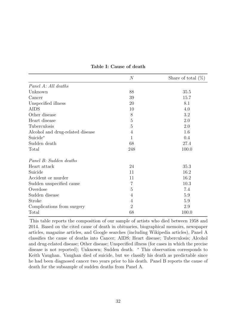
Table I: Cause of death

N Share of total (%)

Panel A: All deathsUnknown 88 35.5Cancer 39 15.7Unspecified illness 20 8.1AIDS 10 4.0Other disease 8 3.2Heart disease 5 2.0Tuberculosis 5 2.0Alcohol and drug-related disease 4 1.6Suicide∗ 1 0.4Sudden death 68 27.4Total 248 100.0

Panel B: Sudden deathsHeart attack 24 35.3Suicide 11 16.2Accident or murder 11 16.2Sudden unspecified cause 7 10.3Overdose 5 7.4Sudden disease 4 5.9Stroke 4 5.9Complications from surgery 2 2.9Total 68 100.0

This table reports the composition of our sample of artists who died between 1958 and2014. Based on the cited cause of death in obituaries, biographical memoirs, newspaperarticles, magazine articles, and Google searches (including Wikipedia articles), Panel Aclassifies the cause of deaths into Cancer; AIDS; Heart disease; Tuberculosis; Alcoholand drug-related disease; Other disease; Unspecified illness (for cases in which the precisedisease is not reported); Unknown; Sudden death. ∗ This observation corresponds toKeith Vaughan. Vaughan died of suicide, but we classify his death as predictable sincehe had been diagnosed cancer two years prior to his death. Panel B reports the cause ofdeath for the subsample of sudden deaths from Panel A.

32

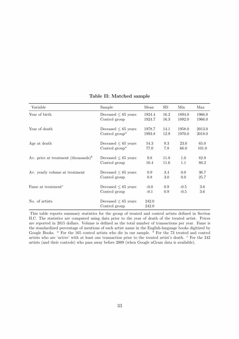
Table II: Matched sample

Variable Sample Mean SD Min Max

Year of birth Deceased ≤ 65 years 1924.4 16.2 1894.0 1966.0Control group 1924.7 16.3 1892.0 1966.0

Year of death Deceased ≤ 65 years 1978.7 14.1 1958.0 2013.0Control groupa 1993.8 12.9 1970.0 2018.0

Age at death Deceased ≤ 65 years 54.3 9.3 23.0 65.0Control groupa 77.0 7.8 66.0 101.0

Av. price at treatment (thousands)b Deceased ≤ 65 years 9.8 11.8 1.0 82.9Control group 10.4 11.6 1.1 80.2

Av. yearly volume at treatment Deceased ≤ 65 years 0.9 3.4 0.0 36.7Control group 0.8 3.0 0.0 25.7

Fame at treatmentc Deceased ≤ 65 years -0.0 0.9 -0.5 3.6Control group -0.1 0.9 -0.5 3.6

No. of artists Deceased ≤ 65 years 242.0Control group 242.0

This table reports summary statistics for the group of treated and control artists defined in SectionII.C. The statistics are computed using data prior to the year of death of the treated artist. Pricesare reported in 2015 dollars. Volume is defined as the total number of transactions per year. Fame isthe standardized percentage of mentions of each artist name in the English-language books digitized byGoogle Books. a For the 165 control artists who die in our sample. b For the 73 treated and controlartists who are ‘active’ with at least one transaction prior to the treated artist’s death. c For the 242artists (and their controls) who pass away before 2009 (when Google nGram data is available).

33

Table III: Impact of artist death on prices and volume – Matched sample

With control group Without control group

Panel A: Death and auction pricesDeceased ≤65 years 0.436 0.277t-stat (3.88) (2.11)Year and age fixed effects and hed. controls Y YArtist fixed effects Y YNo. of observations 57,997 37,178No. of artists (treated + matched controls) 72+72 72

Panel B: Death and volumeDeceased ≤65 years 0.490 0.437t-stat (3.34) (2.99)Year and age fixed effects Y YArtist fixed effects Y YNo. of observations 26,865 13,449No. of artists (treated + matched controls) 242+242 242

This table shows the β1-coefficients in Equations (1)-(2). The sample consists of artistswho passed away at the age of 65 or earlier together with their matched controls (leftcolumn). We also report estimates with treated artists only in the right column. PanelA gives OLS estimates of a regression of log real auction prices on the treatment dummy,while controlling for year, age and individual fixed effects, two dummies proxying fornotoriety (a dummy equal to one when the artist had exhibited at the Documenta andanother one when the artist has sold at least once at Sotheby’s or Christie’s in London orNew York), and the full set of controls to address artwork heterogeneity (medium, auctionhouse, a dummy equal to one if the artwork is signed, a dummy equal to one if the artworkis dated, artwork height and width). Panel B gives conditional quasi-maximum likelihoodPoisson estimates of a regression of annual trading volume on the same set of controls(minus artwork-specific controls). Note the smaller number of artists in Panel A thanin Panel B; measuring the death effect on art price requires that artists are active onthe auction market before their death, hence the smaller sample. Standard errors areclustered at the artist level.

34

Table IV: Turnover elasticity of price

Elasticity Source

Panel A: Art Sample

Average float change of early death ∆f −0.50 Authors’s calculation

Average log price change ∆p 0.46 Table III

Average log volume change ∆v 0.49 Table III

Float elasticity of price εfp = ∆p∆f

−0.92

Float elasticity of volume εfv = ∆v∆f

−0.98

Float elasticity of turnover εft = εfv − 1 −1.98

Turnover elasticity of price εtp = ∆p∆t

=εfpεft

0.46

Panel B: Related Studies

Turnover elasticity of price εtp 0.38 Cochrane (2003) (Table 3)

Turnover elasticity of price εtp 0.24 Xiong and Yu (2011) and

authors’s calculation.

35

Table V: Impact of artist death on prices and volume – Full sample

Unmatched Withoutcontrol group control group

Panel A: Death and auction pricesDeceased ≤65 years 0.415 0.246t-stat (3.98) (1.86)Year and age fixed effects and hed. controls Y YArtist fixed effects Y YNo. of observations 694,071 41,576No. of artists (treated + all controls) 76+2160 76

Panel B: Death and volumeDeceased ≤65 years 0.479 0.460t-stat (3.05) (3.20)Year and age fixed effects Y YArtist fixed effects Y YNo. of observations 124,273 13,657No. of artists (treated + all controls) 246+1990 246

This table shows the β1-coefficients in Equations (1)-(2). The sample consists of all artistsalive at the beginning of the sample period (1957) or later. We also report estimates withtreated artists only in the right column. Panel A gives OLS estimates of a regression of logreal auction prices on the treatment dummy, while controlling for year, age and individualfixed effects, two dummies proxying for notoriety (a dummy equal to one when the artisthad exhibited at the Documenta and another one when the artist has sold at least onceat Sotheby’s or Christie’s in London or New York), and the full set of controls to addressartwork heterogeneity (medium, auction house, a dummy equal to one if the artwork issigned, a dummy equal to one if the artwork is dated, artwork height and width). PanelB gives conditional quasi-maximum likelihood Poisson estimates of a regression of annualtrading volume on the same set of controls (minus artwork-specific controls). Standarderrors are clustered at the artist level.

36

Table VI: Impact of artist death on prices and volume – Alternative controlfor notioriety (1957-2008)




This table shows the β1-coefficients in Equations (1)-(2). Similarly to Table III, thesample consists of artists who passed away at the age of 65 or earlier together with theirmatched controls (left column). The sample stops in 2008 because our Fame control isonly available through 2008. We also report estimates with treated artists only in theright column. Panel A gives OLS estimates of a regression of log real auction priceson the treatment dummy, with a similar set of controls as in Table III, to which weadd an alternative definition of notioriety (as measured by the percentage of mentionsof each artist name in the English-language books digitized by Google Books). Panel Bgives conditional quasi-maximum likelihood Poisson estimates of a regression of annualtrading volume on the same set of controls (minus artwork-specific controls). Standarderrors are clustered at the artist level.

37

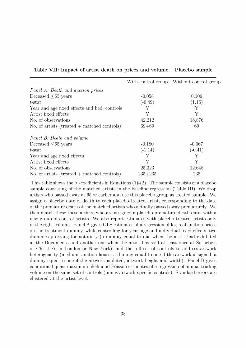
Table VII: Impact of artist death on prices and volume – Placebo sample


Panel A: Death and auction pricesDeceased ≤65 years -0.058 0.106t-stat (-0.49) (1.16)Year and age fixed effects and hed. controls Y YArtist fixed effects Y YNo. of observations 42,212 18,876No. of artists (treated + matched controls) 69+69 69

Panel B: Death and volumeDeceased ≤65 years -0.180 -0.067t-stat (-1.14) (-0.41)Year and age fixed effects Y YArtist fixed effects Y YNo. of observations 25,323 12,648No. of artists (treated + matched controls) 235+235 235

This table shows the β1-coefficients in Equations (1)-(2). The sample consists of a placebosample consisting of the matched artists in the baseline regression (Table III). We dropartists who passed away at 65 or earlier and use this placebo group as treated sample. Weassign a placebo date of death to each placebo-treated artist, corresponding to the dateof the premature death of the matched artists who actually passed away prematurely. Wethen match these these artists, who are assigned a placebo premature death date, with anew group of control artists. We also report estimates with placebo-treated artists onlyin the right column. Panel A gives OLS estimates of a regression of log real auction priceson the treatment dummy, while controlling for year, age and individual fixed effects, twodummies proxying for notoriety (a dummy equal to one when the artist had exhibitedat the Documenta and another one when the artist has sold at least once at Sotheby’sor Christie’s in London or New York), and the full set of controls to address artworkheterogeneity (medium, auction house, a dummy equal to one if the artwork is signed, adummy equal to one if the artwork is dated, artwork height and width). Panel B givesconditional quasi-maximum likelihood Poisson estimates of a regression of annual tradingvolume on the same set of controls (minus artwork-specific controls). Standard errors areclustered at the artist level.

38

Table VIII: Impact of artist death on prices and volume – Sudden deaths




This table shows the β1-coefficients in Equations (1)-(2). The sample consists of artistswho suddenly passed away at the age of 65 or earlier together with their matched con-trols (left column). We report characteristics of the sudden death sample in Table I.We also report estimates with treated artists only in the right column. Panel A givesOLS estimates of a regression of log real auction prices on the treatment dummy, whilecontrolling for year, age and individual fixed effects, two dummies proxying for notoriety(a dummy equal to one when the artist had exhibited at the Documenta and another onewhen the artist has sold at least once at Sotheby’s or Christie’s in London or New York),and the full set of controls to address artwork heterogeneity (medium, auction house, adummy equal to one if the artwork is signed, a dummy equal to one if the artwork isdated, artwork height and width). Panel B gives conditional quasi-maximum likelihoodPoisson estimates of a regression of annual trading volume on the same set of controls(minus artwork-specific controls). Standard errors are clustered at the artist level.

39

Table IX: Impact of artist death on prices and volume – Conditioning on Fameat Death (1957-2008)

High Fame Low Fame

Panel A: Death and auction pricesDeceased ≤65 years 0.599 -0.224t-stat (4.57) (-1.42)Year and age fixed effects and hed. controls Y YArtist fixed effects Y YNo. of observations 45,385 2,480No. of artists (treated + matched controls) 24+24 24+24

Panel B: Death and volumeDeceased ≤65 years 0.586 0.029t-stat (2.87) (0.12)Year and age fixed effects Y YArtist fixed effects Y YNo. of observations 8,815 7,629No. of artists (treated + matched controls) 81+81 81+81

This table shows the β1-coefficients in Equations (1)-(2). Similarly to Table III, thesample consists of artists who passed away at the age of 65 or earlier together withtheir matched controls. The left/right column shows results for artist which Fame (asmeasured by the percentage of mentions of each artist name in the English-languagebooks digitized by Google Books) is within the top/bottom tercile at the year of theirdeath. The sample stops in 2008 because our Fame data is only available through 2008.Panel A gives OLS estimates of a regression of log real auction prices on the treatmentdummy, with a similar set of controls as in Table III. Panel B gives conditional quasi-maximum likelihood Poisson estimates of a regression of annual trading volume on thesame set of controls (minus artwork-specific controls). Standard errors are clustered atthe artist level.

40

Table X: Impact of artist death on volume – Controlling for artist prices

High Fame Low Fame

δi,t 0.168 0.138t-stat (3.59) (1.99)Deceased ≤65 years 0.458 0.420t-stat (3.48) (3.14)Year and age fixed effects Y YArtist fixed effects Y YNo. of observations 4,993 2,467No. of artists (treated + matched controls) 72+72 72

This table shows the β1-coefficients in Equation (2), while controlling for the averageprice of items sold for each artist-year. The sample consists of active artists who passedaway at the age of 65 or earlier together with their matched controls (left column). Wealso report estimates with treated artists only in the right column. The log artist priceindex δi, t is constructed according to Eq. (3) and is linearly interpolated in the absenceof trading volume for a given artist-year. Standard errors are clustered at the artist level.

Table XI: Impact of artist death on round-trip returns


Died ≤ 65 during round-trip 0.477 0.392t-stat (2.15) (1.71)Deceased ≤ 65 at purchase 0.028 0.007t-stat (0.49) (0.05)Year and age fixed effects and hed. controls Y YIndividual fixed effects Y YNo. of observations 764 442No. of artists (treated + controls) 70+72 70

This table shows the β1- and β2− coefficients in Equation (4). The first coefficientmeasures the death effect, similarly to our hedonic specification (1). The β2 coefficienttests whether treated artists earn different returns after their death. The sample consistsof repeat-sales for artists who passed away at the age of 65 or earlier, as well as theirmatched controls (left column). We also report estimates with treated artists only in theright column. Standard errors are clustered at the artist level.

41

Figure 1: Distribution of premature death eventsThis figure depicts the number of artists who died a the age of 65 or earlier in a specificyear over our time span 1958-2014. The total sample of artists who died prematurelyover our sample window (1957-2016) amounts to 258. In order to analyze the impact ofdeath on prices and returns, we require at least one year of price data before an after thedeath in our sample window.

42

(a) Prices

(b) Volume

Figure 2: The death effect declines with the age at death

Panels (a) and (b) present the point estimates and 95% confidence intervals for the causalimpact of death interacted with the age at death. The sample includes all artists whoare alive at the beginning of our sample period (1957). Panel (a) gives OLS estimates(based on Equation (1)); Panel (b) gives QML Poisson estimates (based on Equation(2)). Standard errors are clustered at the artist level.

43

(a) Prices

(b) Volume

Figure 3: Prices and trading volume around year of death

Panels (a) and (b) present the point estimates and 95% confidence intervals for the causalimpact of death in a given year relative to the artist’s death. The sample includes alltreated artists who are active prior to their death. Panel (a) gives OLS estimates (basedon Equation (1)); Panel (b) gives QML Poisson estimates (based on Equation (2)), similarto Column 1 of Table III. Observations more than 5 (10) years before (after) the deathare grouped together. Standard errors are clustered at the artist level.

44

Appendix – For Online Publication

Matched Sample

Treated artists ControlsArtist Birth Death Active Artist Birth Death

Aagaard Andersen, Gunnar 1919 1982 Lassnig, Maria 1919 2014Abedin, Zainul 1914 1976 Hogan, Joao 1914 1988Afro 1912 1976 Y Soulages, Pierre 1919 –Ali, Shakir 1916 1975 Heyboer, Anton 1924 2005Altenbourg, Gerhard 1926 1989 Y Trujillo, Guillermo 1927 –Angus, Rita 1908 1970 Korniss, Dezso 1908 1984Apap, William 1918 1970 Quiros, Antonio 1918 1984Arbus, Diane 1923 1971 Bury, Pol 1922 2005Arkley, Howard 1951 1999 Y Oulton, Therese 1953 –Atlan, Jean-Michel 1913 1960 Butler, Reg 1913 1981Ayrton, Michael 1921 1975 Y Johnson, Ray 1927 1995Baldessin, George 1939 1978 Y Attersee, Christian Ludwig 1940 –Bandeira, Antonio 1922 1967 Cruz-Diez, Carlos 1923 –Batlle Planas, Juan 1911 1966 Paniker, K. C. S. 1911 1977Bazile, Castera 1923 1966 Palacios, Luisa 1923 1990Baziotes, William 1912 1963 Burri, Alberto 1915 1995Bela 1917 1968 Hare, David 1917 1992Belkin, Arnold 1930 1992 Y Felguerez, Manuel 1928 –Beuys, Joseph 1921 1986 Y Pearlstein, Philip 1924 –Binyinyiwuy 1928 1982 Imai, Toshimitsu 1928 2002Birolli, Renato 1905 1959 Porter, Fairfield 1907 1975Boetti, Alighiero 1940 1994 Onobrakpeya, Bruce 1932 –Bogusz, Marian 1920 1980 Castro, Amilcar de 1920 2002Bonevardi, Marcelo 1929 1994 Y Saul, Peter 1934 –Borduas, Paul-Emile 1905 1960 Cremer, Fritz 1906 1993Brauner, Victor 1903 1966 Krasner, Lee 1908 1984Bredow, Rudolf 1909 1973 Bergman, Anna-Eva 1909 1987Brittain, Miller 1912 1968 Spyropoulos, Yannis 1912 1990Broodthaers, Marcel 1924 1976 Neri, Manuel 1930 –Brown, Joan 1938 1990 Weiner, Lawrence 1942 –Brown, Mike 1938 1997 Y Jaray, Tess 1937 –Bruning, Peter 1929 1970 Larter, Richard 1929 2014Buthe, Michael 1944 1994 Y McLean, Bruce 1944 –Caballero, Luis 1943 1995 Y Mosset, Olivier 1944 –Campbell, George 1917 1979 Y Rodhe, Lennart 1916 2005Carrillo, Lilia 1930 1974 Claus, Carlfriedrich 1930 1998Castagnino, Juan Carlos 1908 1972 Stematsky, Avigdor 1908 1989Chaissac, Gaston 1910 1964 Lamba, Jacqueline 1910 1993Chambers, Jack 1931 1978 Comtois, Ulysse 1931 1999Cherkaoui, Ahmed 1934 1967 Gaucher, Yves 1934 2000Chighine, Alfredo 1914 1974 Y Messagier, Jean 1920 1999Christensen, Dan 1942 2007 Y Self, Colin 1941 –Chukwuogo-Roy, Chinwe 1952 2012 Von Hausswolff, C. M. 1956 –Colquhoun, Robert 1914 1962 Schumacher, Emil 1912 1999Corbett, Edward 1919 1971 Abreu, Mario 1919 1993

A1

Coronel, Pedro 1923 1985 Y Colville, Alex 1920 2013Corzas, Francisco 1936 1983 Y Chavez, Gerardo 1937 –Crippa, Roberto 1921 1972 Y Sugai, Kumi 1919 1996Curnoe, Greg 1936 1992 Gershuni, Moshe 1936 2017Cutrone, Ronnie 1948 2013 Y Cahn, Miriam 1949 –Dallaire, Jean 1916 1965 Badii, Libero 1916 2001Daraniyagala, Justin Pieris 1903 1967 Wang Xuetao 1903 1982Davies, John 1936 1999 Y Goode, Joe 1937 –Davis, Gene 1920 1985 Y Carrington, Leonora 1917 2011Defeo, Jay 1929 1989 Beksinski, Zdzislaw 1929 2005Deira, Ernesto 1928 1986 Y Makowski, Zbigniew 1930 –Dekkers, Ad 1938 1974 Lancaster, Mark 1938 –Deyrolle, Jean 1911 1967 Orlando, Felipe 1911 2001Diller, Burgoyne 1906 1965 Aeschbacher, Hans 1906 1980Disney, Walt 1901 1966 Turner, Helen Monro 1901 1977Djanira 1914 1979 Guerrero, Jose 1914 1991Dotremont, Christian 1922 1979 Day, Melvin 1923 2016Downey, Juan 1940 1993 Attersee, Christian Ludwig 1940 –Dumouchel, Albert 1916 1971 Gysin, Brion 1916 1986Duwe, Harald 1926 1984 Johnson, George Henry 1926 2007Eardley, Joan 1921 1963 Raza, Sayed Haider 1922 –Echeverria, Enrique 1923 1972 Hlito, Alfredo 1923 1994Endara Crow, Gonzalo 1936 1996 Y Amaral, Antonio Henrique 1935 2015Engilberts, Jon 1908 1972 Marczynski, Adam 1908 1985Espaliu, Pepe 1955 1993 Nel, Karel Anthony 1955 –Evans, Merlyn 1910 1973 Y Lancaster, Osbert 1908 1986Eyuboglu, Bedri Rahmi 1911 1975 Lardera, Berto 1911 1989Fahlstrom, Oyvind 1928 1976 Scott, Patrick 1921 2014Fairhurst, Angus 1966 2008 Y Paine, Roxy 1966 –Farrell, Micheal 1940 2000 Y Wilson, Robert 1941 –Feeley, Paul 1910 1966 Mortensen, Richard 1910 1993Feni, Dumile 1942 1991 Bruggen, Coosje van 1942 2009Fernhout, Edgar 1912 1974 Cage, John 1912 1992Ferren, John 1905 1970 Cadmus, Paul 1904 1999Fisher, Sandra 1947 1994 Y Lavier, Bertrand 1949 –Flavin, Dan 1933 1996 Y Buren, Daniel 1938 –Fomison, Tony 1939 1990 Y Polesello, Rogelio 1939 2014Forg, Gunther 1952 2013 Y Scharf, Kenny 1958 –Fraile, Alfonso 1930 1988 Y Brizzi, Ary 1930 2014Freedman, Barnett 1901 1958 Johnson, William H. 1901 1970Frink,Elisabeth 1930 1993 Y Cuevas, Jose Luis 1934 –Fruhtrunk, Gunter 1923 1982 Y Kupferman, Moshe 1926 2003Fu Baoshi 1904 1965 Messel, Oliver 1904 1978Gadanyi, Jeno 1896 1960 Adalid, Agustin Lazo 1896 1971Galan, Julio 1958 2006 Y Currie, Ken 1960 –Garcia Ponce, Fernando 1933 1987 Molinari, Guido 1933 2004Gnoli, Domenico (ii) 1933 1970 Ferrer, Rafael 1933 –Goldstein, Jack 1945 2003 Y Nerdrum, Odd 1944 –Gonzales-Torres, Felix 1957 1996 Sitthiket, Vasan 1957 –Gonzalez, Juan 1945 1993 Piper, Adrian 1948 –Graves, Nancy 1939 1995 Hiller, Susan 1940 –Greco, Alberto 1931 1965 Baya 1931 1998

A2

Grundig, Hans 1901 1958 Evergood, Philip 1901 1973Grunwald, Henryk 1904 1958 Mason, Alice Trumbull 1904 1971Guerrero Galvan, Jesus 1910 1973 Sterne, Hedda 1910 2011Gundersen, Gunnar S. 1921 1983 Garcia Guerrero, Luis 1921 1996Hardin, Helen 1943 1984 Rosler, Martha 1943 –Haring, Keith 1958 1990 Y Paladino, Mimmo 1948 –Hennessy, Patrick 1915 1980 Dzubas, Friedel 1915 1994Hesse, Eva 1936 1970 Ono, Yoko 1933 –Hester, Joy 1920 1960 Gonzalez Bogen, Carlos 1920 1992Hilton, Roger 1911 1975 Y Schultze, Bernard 1915 2005Hockelmann, Antonius 1937 2000 Y Max, Peter 1937 –Hung, Francisco 1937 2001 Y Senbergs, Jan 1939 –Immendorff, Jorg 1945 2007 Y Fetting, Rainer 1949 –Jacoulet, Paul 1896 1960 Rodriguez Lozano, Manuel 1896 1971Jarema, Maria 1908 1958 Aroch, Arie 1908 1974Jarman, Derek 1942 1994 Y Petrick, Wolfgang 1939 –John, Jiri 1923 1972 Kemble, Kenneth 1923 1998Jones, Joe 1909 1963 Stromme, Olav 1909 1978Jorn, Asger 1914 1973 Y Friend, Donald 1914 1989Kazuki, Yasuo 1911 1974 Benoit, Rigaud 1911 1986Kelley, Mike 1954 2012 Y Sherman, Cindy 1954 –Kemeny, Zoltan 1907 1965 Kotin, Albert 1907 1980Kenny, Michael 1941 1999 Y Pacheco, Ana-Maria 1943 –Kim Hwan-gi 1913 1974 Oppenheim, Meret 1913 1985King, Cecil 1921 1986 Espinola Gomez, Manuel 1921 2003Kinley, Peter 1926 1988 Y Skotnes, Cecil 1926 2009Kippenberger, Martin 1953 1997 Y Schutte, Thomas 1954 –Klein, Yves 1928 1962 Leslie, Alfred 1927 –Kline, Franz 1910 1962 Graves, Morris 1910 2001Kobzdej, Aleksander 1920 1972 Barcala, Washington 1920 1993Kondor, Bela 1931 1972 Coughtry, Graham 1931 1999Kudo, Tetsumi 1935 1990 Y Rodriguez, Alirio 1934 2018Kurelek, William 1927 1977 Y Rainer, Arnulf 1929 –Lanyon, Peter 1918 1964 Johnson, Lester 1919 2010Lasekan, Akinola 1916 1972 Thieler, Fred 1916 1999Lavonen, Ahti 1928 1970 Swaminathan, Jagdish 1928 1994Ledy, Cheik 1962 1997 Yuskavage, Lisa 1962 –Leura Tjapaltjarri, Tim 1929 1984 Metzkes, Harald 1929 –Licini, Osvaldo 1894 1958 Reggiani, Mauro 1897 1980Lo Savio, Francesco 1935 1963 Sihlali, Durant 1935 2004Louis, Morris 1912 1962 Guttuso, Renato 1911 1987Lueg, Konrad 1939 1996 Y Donaldson, Anthony 1939 –Lui Shou-kwan 1919 1975 Walters, Gordon 1919 1995Lunar, Emerio 1940 1990 Coen, Arnaldo 1940 –MacBryde, Robert 1913 1966 Gopas, Rudolf 1913 1983Macdonald, Jock 1897 1960 Yirawala 1897 1976Mafai, Mario 1902 1965 Sternberg, Harry 1904 2001Magani, Mick 1920 1984 Muller, Robert 1920 2003Malaval, Robert 1937 1980 Suarez, Pablo 1937 2006Manzoni, Piero 1933 1963 Katz, Alex 1927 –Mapplethorpe, Robert 1946 1989 Anderson, Laurie 1947 –Marika, Mawalan 1908 1967 Camarena, Jorge Gonzalez 1908 1980

A3

Marika, Wandjuk 1927 1987 Malangi, David 1927 1999Martin, Mary 1907 1969 Bill, Max 1908 1994Matta-Clark, Gordon 1943 1978 Turrell, James 1943 –Maymurru, Narritjin 1916 1981 Palazuelo, Pablo 1916 2007McHale, John 1922 1978 Niro, Robert de, Sr. 1922 1993Medek, Mikulas 1926 1974 Capdevila, F. M. 1926 1995Mendieta, Ana 1948 1985 Abramovic, Marina 1946 –Messil, Gabriel 1934 1986 Khakhar, Bhupen 1934 2003Millares, Manolo 1926 1972 Aitchison, Craigie 1926 2009Milpurrurru, George 1934 1998 Y Cohen, Bernard 1933 –Minaux, Andre 1923 1986 Y Renqvist, Torsten 1924 2007Mithinari 1929 1976 Gironella, Alberto 1929 1999Moke 1950 2001 Y Coe, Sue 1951 –Molvig, Jon 1923 1970 Alonso, Raul 1923 1993Morton, Ree 1936 1977 Wakabayashi, Isamu 1936 2003Mualla, Fikret 1903 1967 Rimsa, Juan 1903 1978Munoz, Juan 1953 2001 Y Leirner, Jac 1961 –Namatjira, Albert 1902 1959 Carter, Clarence Holbrook 1904 2000Nanninga, Jaap 1904 1962 Burra, Edward 1905 1976Newman, Barnett 1905 1970 Motherwell, Robert 1915 1991Nickolls, Trevor 1949 2012 Y Koningsbruggen, Rob van 1948 –Oiticica, Helio 1937 1980 Brawley, Robert J 1937 2006Ojeda, Gustavo 1958 1989 Y Favier, Phillipe 1957 –Onus, Lin 1948 1996 Woodrow, Bill 1948 –Orszag, Lili 1926 1978 Thomas, Rover 1926 1998Paalen, Wolfgang 1905 1959 Tworkov, Jack 1900 1982Pacheco, Maria Luisa 1919 1982 Y Lataster, Ger 1920 2012Palermo, Blinky 1943 1977 Marioni, Joseph 1943 2009Pancetti, Jose Gianini 1902 1958 Stokes, Adrian 1902 1972Pane, Gina 1939 1990 Alviani, Getulio 1939 2018Park, David 1911 1960 Mariano 1912 1980Parvez, Ahmed 1926 1979 Ronald, William 1926 1998Paschke, Ed 1939 2004 Y Knoebel, Imi 1940 –Pedro, Antonio 1909 1966 Lewis, Norman 1909 1979Peeters, Jozef 1895 1960 Maxy, Max Herman 1895 1971Pike, Jimmy 1940 2002 Y Revilla, Carlos 1940 –Poliakoff, Serge 1906 1969 Y Manessier, Alfred 1911 1993Ponc, Joan 1927 1984 Rivera, Manuel 1927 1995Popkov, Viktor 1932 1974 Uglow, Euan 1932 2000Portinari, Candido 1903 1962 Clifton, Marshall 1903 1975Potworowski, Piotr 1898 1962 Y Zack, Leon 1892 1980Preller, Alexis 1911 1975 Y Meistermann, Georg 1911 1990Reinhardt, Ad 1913 1967 Smith, Tony 1912 1980Requichot, Bernard 1929 1961 Munoz, Lucio 1929 1998Rhoades, Jason 1965 2006 Bulloch, Angela 1966 –Richier, Germaine 1902 1959 Herrera, Velino 1902 1973Sadequain 1930 1987 Pomodoro, Gio 1930 2002Sage, Kay 1898 1963 Feng Zikai 1898 1975Schwalbe, Ole 1929 1990 Y Hrdlicka, Alfred 1928 2009Seitz, Gustav 1906 1969 Baij, Ramkinker 1906 1980Seligmann, Kurt 1900 1962 Woodruff, Hale 1900 1980Sempere, Eusebio 1923 1985 Cesariny, Mario 1923 2006

A4

Serpa, Ivan 1923 1973 Jess (Collins, Burgess) 1923 2004Shi Lu 1919 1982 Yamamoto, Taro 1919 1994Silva, Carlos 1930 1987 Eggenschwiler, Franz 1930 2000Skold, Otte 1894 1958 Bernath, Aurel 1895 1982Smith, David 1906 1965 Brooks, James 1906 1992Smithson, Robert 1938 1973 Bell, Larry 1939 –Sokolov-Skalya, Pavel 1899 1961 Glarner, Fritz 1899 1972Stajuda, Jerzy 1936 1992 Golden, Daan van 1936 2017Stankiewicz, Richard 1922 1983 Velarde, Pablita 1918 2006Stepanova, Varvara 1894 1958 Centurion, Emilio 1894 1970Stohrer, Walter 1937 2000 Y Iseli, Rolf 1934 –Swift, Patrick 1927 1983 Daws, Lawrence 1927 –Takamatsu, Jiro 1936 1998 Y Schonebeck, Eugen 1936 –Taylor, E. Mervyn 1906 1964 Grundig, Lea 1906 1977Thek, Paul 1933 1988 Tousignant, Claude 1932 –Thomkins, Andre 1930 1985 Y Tubke, Werner 1929 2004Thompson, Bob 1937 1966 Scholder, Fritz 1937 2005Tschusiya, Tilsa 1928 1984 Fernandez, Agustin 1928 2006Tsingos, Thanos 1914 1965 Balint, Endre 1914 1986Tuckson, Tony 1921 1973 Iskowitz, Gershon 1921 1988Valcin, Gerard 1927 1988 Y Guinovart, Josep 1927 2007Varo, Remedios 1908 1963 Lewers, Margo 1908 1978Vassilieff, Danila 1897 1958 Pan Tianshou 1897 1971Vaughan, Keith 1912 1977 Y Turcato, Giulio 1912 1995Vega, Jorge de la 1930 1971 D’Arcangelo, Allan 1930 1998Vordemberge-Gildewart, F. 1899 1962 Carvalho, Flavio de 1899 1973Warhol, Andy 1928 1987 Y Riopelle, Jean-Paul 1923 2002West, Franz 1947 2012 Y Neshat, Shirin 1957 –White, Charles Wilbert 1918 1979 Solari, Luis 1918 1993Whiteley, Brett 1939 1992 Y Kirkeby, Per 1938 –Wiedemann, Guillermo 1905 1969 Narvaez, Francisco 1905 1982Wilke, Hannah 1940 1993 Armajani, Siah 1939 –Wilkerson, Jerry 1943 2007 Y Buraimoh, Jimoh 1943 –Williams, Fred 1927 1982 Y Fuchs, Ernst 1930 –Wlodarski, Marek 1903 1960 Bodmer, Walter 1903 1973Wojnarowicz, David 1954 1992 Y Frize, Bernard 1954 –Woodman, Francesca 1958 1981 Wiszniewski, Adrian 1958 –Wunuwun, Jack 1930 1990 Jaimes Sanchez, Humberto 1930 2003Zabaleta, Rafael 1907 1960 Yunapingu, Munggurrawuy 1907 1979Zobel, Fernando 1924 1984 Morellet, Francois 1926 2016Zverev, Anatoly 1931 1986 Opalka, Roman 1931 2011

A5

Tilburg University When a Master Dies Penasse, Julien ...

Documents

Transcript of Tilburg University When a Master Dies Penasse, Julien ...