Clemson UniversityTigerPrints

All Dissertations Dissertations

5-2016

Generalized Colorings of GraphsHonghai XuClemson University, honghax@g.clemson.edu

Follow this and additional works at: https://tigerprints.clemson.edu/all_dissertations

This Dissertation is brought to you for free and open access by the Dissertations at TigerPrints. It has been accepted for inclusion in All Dissertations byan authorized administrator of TigerPrints. For more information, please contact kokeefe@clemson.edu.

Recommended CitationXu, Honghai, "Generalized Colorings of Graphs" (2016). All Dissertations. 1650.https://tigerprints.clemson.edu/all_dissertations/1650

GENERALIZED COLORINGS OF GRAPHS

A Dissertation

Presented to

the Graduate School of

Clemson University

In Partial Fulfillment

of the Requirements for the Degree

Doctor of Philosophy

Mathematical Sciences

by

Honghai Xu

May 2016

Accepted by:

Dr. Wayne Goddard, Committee Chair

Dr. Michael Burr

Dr. Gretchen Matthews

Dr. Beth Novick

Abstract

A graph coloring is an assignment of labels called “colors” to certain elements of

a graph subject to certain constraints. The proper vertex coloring is the most common

type of graph coloring, where each vertex of a graph is assigned one color such that no

two adjacent vertices share the same color, with the objective of minimizing the number of

colors used. One can obtain various generalizations of the proper vertex coloring problem,

by strengthening or relaxing the constraints or changing the objective. We study several

types of such generalizations in this thesis.

Series-parallel graphs are multigraphs that have no K4-minor. We provide bounds

on their fractional and circular chromatic numbers and the defective version of these pa-

rameters. In particular we show that the fractional chromatic number of any series-parallel

graph of odd girth k is exactly 2k/(k − 1), confirming a conjecture by Wang and Yu.

We introduce a generalization of defective coloring: each vertex of a graph is assigned

a fraction of each color, with the total amount of colors at each vertex summing to 1. We

define the fractional defect of a vertex v to be the sum of the overlaps with each neighbor

of v, and the fractional defect of the graph to be the maximum of the defects over all vertices.

We provide results on the minimum fractional defect of 2-colorings of some graphs. We also

propose some open questions and conjectures.

Given a (not necessarily proper) vertex coloring of a graph, a subgraph is called

rainbow if all its vertices receive different colors, and monochromatic if all its vertices receive

the same color. We consider several types of coloring here: a no-rainbow-F coloring of G

ii

is a coloring of the vertices of G without rainbow subgraph isomorphic to F ; an F -WORM

coloring of G is a coloring of the vertices of G without rainbow or monochromatic subgraph

isomorphic to F ; an (M,R)-WORM coloring of G is a coloring of the vertices of G with

neither a monochromatic subgraph isomorphic to M nor a rainbow subgraph isomorphic to

R. We present some results on these concepts especially with regards to the existence of

colorings, complexity, and optimization within certain graph classes. Our focus is on the

case that F , M or R is a path, cycle, star, or clique.

iii

Dedication

This thesis is dedicated to Melody Siyun Xu.

iv

Acknowledgments

I thank my research advisor Wayne Goddard for his guidance and dedication, and

for his tremendous help in every aspect of my career. It has been a wonderful and beneficial

experience working with him, and this thesis would not have been possible without his

guidance. I also thank the other members of my PhD committee, Michael Burr, Gretchen

Matthews, and Beth Novick, for offering lots of helpful advice and comments on this thesis.

Thanks to K.B. Kulasekera for teaching me a course in probability, and for giving

me an opportunity to earn my teaching assistantship.

Thanks to Herve Kerivin for his encouragement, and for teaching me linear pro-

gramming and discrete optimization.

Thanks to Douglas Shier for teaching me network flow programming, and for his

kind help with my job search.

Thanks to Allen Guest for his kind help with my teaching and job search.

I would like to thank my father Xilin Xu, my mother Yiping Yu, my mother-in-law

Zhi Li, and my father-in-law Xiaogang Tian, for their constant support.

Last but not the least, I cannot express how grateful I am to my wife Ye Tian for her

continuous encouragement and unconditional support along the way, and will never forget

how she drove me from Columbia to Clemson so that I could save time and prepare for my

prelim exam in the car.

v

Table of Contents

Title Page . . . . . . . . . . . . . . . . . . . . . . . . . . . . . . . . . . . . . . . i

Abstract . . . . . . . . . . . . . . . . . . . . . . . . . . . . . . . . . . . . . . . . ii

Dedication . . . . . . . . . . . . . . . . . . . . . . . . . . . . . . . . . . . . . . . iv

Acknowledgments . . . . . . . . . . . . . . . . . . . . . . . . . . . . . . . . . . v

List of Tables . . . . . . . . . . . . . . . . . . . . . . . . . . . . . . . . . . . . . viii

List of Figures . . . . . . . . . . . . . . . . . . . . . . . . . . . . . . . . . . . . . ix

1 Introduction . . . . . . . . . . . . . . . . . . . . . . . . . . . . . . . . . . . . 11.1 Definitions and Notations . . . . . . . . . . . . . . . . . . . . . . . . . . . . 11.2 Thesis Organization . . . . . . . . . . . . . . . . . . . . . . . . . . . . . . . 6

2 Fractional, Circular, and Defective Coloring of Series-Parallel Graphs . 82.1 Introduction . . . . . . . . . . . . . . . . . . . . . . . . . . . . . . . . . . . . 82.2 Proper Fractional Colorings . . . . . . . . . . . . . . . . . . . . . . . . . . . 112.3 Defective Colorings . . . . . . . . . . . . . . . . . . . . . . . . . . . . . . . . 152.4 Related Questions . . . . . . . . . . . . . . . . . . . . . . . . . . . . . . . . 18

3 Colorings with Fractional Defect . . . . . . . . . . . . . . . . . . . . . . . . 193.1 Introduction . . . . . . . . . . . . . . . . . . . . . . . . . . . . . . . . . . . . 193.2 Preliminaries . . . . . . . . . . . . . . . . . . . . . . . . . . . . . . . . . . . 213.3 Two-Colorings of Some Graph Families . . . . . . . . . . . . . . . . . . . . 243.4 Complexity . . . . . . . . . . . . . . . . . . . . . . . . . . . . . . . . . . . . 37

4 Vertex Colorings without Rainbow Subgraphs . . . . . . . . . . . . . . . 394.1 Introduction . . . . . . . . . . . . . . . . . . . . . . . . . . . . . . . . . . . . 394.2 Preliminaries . . . . . . . . . . . . . . . . . . . . . . . . . . . . . . . . . . . 414.3 Forbidden P3 . . . . . . . . . . . . . . . . . . . . . . . . . . . . . . . . . . . 424.4 Forbidden Triangles . . . . . . . . . . . . . . . . . . . . . . . . . . . . . . . 484.5 Forbidden Stars . . . . . . . . . . . . . . . . . . . . . . . . . . . . . . . . . . 534.6 Conclusion . . . . . . . . . . . . . . . . . . . . . . . . . . . . . . . . . . . . 60

5 WORM Colorings Forbidding Paths . . . . . . . . . . . . . . . . . . . . . 61

vi

5.1 Introduction . . . . . . . . . . . . . . . . . . . . . . . . . . . . . . . . . . . . 615.2 Basics . . . . . . . . . . . . . . . . . . . . . . . . . . . . . . . . . . . . . . . 625.3 Some Calculations . . . . . . . . . . . . . . . . . . . . . . . . . . . . . . . . 655.4 Trees . . . . . . . . . . . . . . . . . . . . . . . . . . . . . . . . . . . . . . . . 705.5 WORM is Easy Sometimes . . . . . . . . . . . . . . . . . . . . . . . . . . . 735.6 Extremal Questions . . . . . . . . . . . . . . . . . . . . . . . . . . . . . . . 74

6 WORM colorings Forbidding Cycles or Cliques . . . . . . . . . . . . . . . 756.1 Introduction . . . . . . . . . . . . . . . . . . . . . . . . . . . . . . . . . . . . 756.2 Forbidding a Triangle . . . . . . . . . . . . . . . . . . . . . . . . . . . . . . 766.3 Forbidding a 4-Cycle or All Cycles . . . . . . . . . . . . . . . . . . . . . . . 816.4 Forbidding a Clique or Biclique . . . . . . . . . . . . . . . . . . . . . . . . . 866.5 Minimal Colorings . . . . . . . . . . . . . . . . . . . . . . . . . . . . . . . . 88

7 Vertex Colorings without Rainbow or Monochromatic Subgraphs . . . . 907.1 Introduction . . . . . . . . . . . . . . . . . . . . . . . . . . . . . . . . . . . . 907.2 Preliminaries . . . . . . . . . . . . . . . . . . . . . . . . . . . . . . . . . . . 927.3 A Result on Rainbow Paths . . . . . . . . . . . . . . . . . . . . . . . . . . . 937.4 Proper Colorings . . . . . . . . . . . . . . . . . . . . . . . . . . . . . . . . . 947.5 Other Results . . . . . . . . . . . . . . . . . . . . . . . . . . . . . . . . . . . 1027.6 Other Directions . . . . . . . . . . . . . . . . . . . . . . . . . . . . . . . . . 103

8 Conclusion and Future Directions of Research . . . . . . . . . . . . . . . 104

Bibliography . . . . . . . . . . . . . . . . . . . . . . . . . . . . . . . . . . . . . . 106

vii

List of Tables

4.1 Extremal values of NRP3(G) for cubic graphs G of fixed order . . . . . . . . 474.2 Maximum values of NRK1,3(G) for maximal outerplanar graphs of fixed order 58

viii

List of Figures

2.1 A series-parallel graph with circular chromatic number 8/3 . . . . . . . . . 102.2 S1 and S3 as subsets of ` colors . . . . . . . . . . . . . . . . . . . . . . . . . 122.3 A series-parallel graph Gk (k ≥ 5) with given odd girth and large d-defective

fractional chromatic number . . . . . . . . . . . . . . . . . . . . . . . . . . . 162.4 The graph H1 whose 1-defective circular chromatic number is 8/3 . . . . . . 17

3.1 An optimal 2-coloring of the Hajos graph . . . . . . . . . . . . . . . . . . . 20

4.1 A graph whose optimal no-rainbow-P3 coloring has a disconnected color class 444.2 The two cubic graphs of order 18 with maximum NRP3 . . . . . . . . . . . 494.3 Part of a maximal outerplanar graph and its weak dual . . . . . . . . . . . 514.4 The cubic graph of order 20 with maximum NRK1,3 . . . . . . . . . . . . . 554.5 A cubic graph of order 14 with minimum NRK1,3 . . . . . . . . . . . . . . . 564.6 Maximal outerplanar graphs with maximum NRK1,3 . . . . . . . . . . . . . 594.7 The maximal outerplanar graph M3 with NRK1,3 = 13 . . . . . . . . . . . . 59

5.1 The graph H4 whose P3-WORM colorings use either 2 or 4 colors . . . . . . 645.2 A cubic graph of order 20 with W+(G,P3) = 6 . . . . . . . . . . . . . . . . 675.3 Two MOPs: the fan F6 and the Hajos graph . . . . . . . . . . . . . . . . . 685.4 A MOP that has no F6 or Hajos subgraph . . . . . . . . . . . . . . . . . . . 69

6.1 Reduction of K3-WORM coloring from NAE-3SAT . . . . . . . . . . . . . . 806.2 The graph having minimum W+(G,C4) over cubic graphs of order 12 . . . 846.3 An optimal C4-WORM coloring of the 6× 6 grid . . . . . . . . . . . . . . . 85

7.1 A cubic graph G with W+(G;K2,K1,3) two-thirds its order . . . . . . . . . 977.2 The known cubic graphs with W+(G;K2,K1,3) = 3 . . . . . . . . . . . . . . 977.3 A nonbipartite graph G with a perfect matching and maximum W+(G;K2, P4) 987.4 Coloring showing W+(C13;K2, P4) . . . . . . . . . . . . . . . . . . . . . . . 997.5 Coloring of Mobius ladder . . . . . . . . . . . . . . . . . . . . . . . . . . . . 102

ix

Chapter 1

Introduction

A graph coloring is an assignment of labels called “colors” to certain elements of a

graph subject to certain constraints. The proper vertex coloring is the most common type

of graph coloring, where each vertex of a graph is assigned one color such that adjacent

vertices receive different colors, with the objective of minimizing the number of colors used.

One can obtain various generalizations of the proper vertex coloring problem, by

strengthening or relaxing the constraints or changing the objective. For example, in a

distance d-coloring (see, for example, [55, 32, 48]), no two vertices within distance d of each

other share the same color; in a defective coloring (see, for example, [20, 21]), a vertex

can receive the same color as some of its neighbors do; in a fractional coloring (see, for

example, [57, 67]), each vertex receives a set of colors instead of one color.

We study several types of such generalizations in this thesis. For comprehensive

surveys of graph coloring problems, we refer readers to [49, 69, 17].

1.1 Definitions and Notations

Our definitions and notations are fairly standard. For additional background and

examples, see [78].

1

A graph G consists of a set V (G) of vertices and a set E(G) of edges, such that each

edge is an unordered pair of distinct vertices; thus, each edge is associated with two vertices

called its endpoints. For brevity we write uv instead of (u, v) for an edge with endpoints u

and v. If uv is an edge, then vertices u and v are adjacent and are neighbors, and they are

each incident to uv. Edges are incident if they have a common endpoint.

More generally, a multigraph G consists of a set V (G) of vertices and a multiset E(G)

of edges, such that each edge is an unordered pair of (not necessarily distinct) vertices. Mul-

tiple edges are edges having the same pair of endpoints. A loop is an edge whose endpoints

are equal. When discussing multigraphs, we may emphasize the absence of multiple edges

and loops by calling a graph a simple graph.

The number of vertices of a graph G is its order. We say a graph is trivial if its

order is 0 or 1. The number of edges of a graph G is its size. We say a graph is empty if its

size is 0. The degree d(v) of a vertex v is the number of edges incident to v. The minimum

degree δ(G) of a graph G is min{d(v)|v ∈ V (G)}. The maximum degree ∆(G) of a graph G

is max{d(v)|v ∈ V (G)}. If every vertex of a graph G has degree k, then G is k-regular. In

particular, a 3-regular graph is also called a cubic graph. A clique in a graph is a set of

pairwise adjacent vertices. The clique number ω(G) of a graph G is the maximum size of a

clique in G. An independent set in a graph is a set of pairwise nonadjacent vertices. The

independence number α(G) of a graph G is the maximum size of an independent set in G.

An isomorphism from a graph G to a graph H is a bijection f : V (G)→ V (H) such

that uv ∈ E(G) if and only if f(u)f(v) ∈ E(H). If there is an isomorphism from G to H,

then we say that G is isomorphic to H, written G ∼= H.

The complement G of a graph G is the graph with vertex set V (G) such that

uv ∈ E(G) if and only if uv /∈ E(G). A graph H is called a subgraph of a graph G if

V (H) ⊆ V (G) and E(H) ⊆ E(G). If H is a subgraph of G and H 6= G, then H is a proper

subgraph of G. If H is a subgraph of G and V (H) = V (G), then H is a spanning subgraph

of G. If H is a subgraph of G, and H contains all the edges uv ∈ E(G) with u, v ∈ V (H),

2

then H is an induced subgraph G; we say that V (H) (or E(H)) induces H. A graph G is

H-free if G has no induced subgraph isomorphic to H. The open neighborhood of a vertex v

in a graph G, written NG(v) or simply N(v), is the subgraph of G induced by all neighbors

of v. The closed neighborhood of a vertex v in a graph G, written NG[v] or simply N [v], is

the subgraph of G induced by v and all neighbors of v.

In a graph G, the subdivision of an edge uv is the operation that replaces uv with a

path u,w, v through a new vertex w; while the contraction of an edge uv, written G/uv, is

the operation that replaces u and v with a new vertex such that the new vertex is incident

to the edges, other than uv, that were incident to u or v. We write G− e for the subgraph

of G obtained by deleting an edge e, and G−M for the subgraph of G obtained by deleting

a set of edges M . We write G − v for the subgraph of G obtained by deleting a vertex v

and all its incident edges, and G − S for the subgraph of G obtained by deleting a set of

vertices S and all their incident edges. A graph H is a minor of G if H can be formed from

G by deleting vertices or edges or by contracting edges. A graph H is a subdivision of G

if H can be formed from G by successive edge subdivisions.

A complete graph is a graph whose vertices are all pairwise adjacent. The complete

graph with n vertices is denoted Kn; in particular, K3 is also called a triangle. A path is

a graph of the form V (G) = {v1, v2, . . . , vn} and E(G) = {v1v2, v2v3, . . . , vn−1vn}, where

n ≥ 1 and the vi are all distinct. The path with n vertices is denoted Pn. A cycle is a graph

of the form V (G) = {v1, v2, . . . , vn} and E(G) = {v1v2, v2v3, . . . , vn−1vn, vnv1}, where n ≥ 3

and the vi are all distinct. The cycle with n vertices is denoted Cn. The number of edges

of a path (or cycle) is called its length. A cyclic graph is a graph that contains a cycle. A

forest (acyclic graph) is a graph that does not contain any cycle. A chord of a cycle C is

an edge not in C whose endpoints lie in C. A chordal graph is a graph in which all cycles

with four or more vertices have a chord. Equivalently, every induced cycle in the graph has

at most three vertices.

A graph G is connected if there is a path between every pair of distinct vertices of G.

3

The components of a graph are its maximal connected subgraphs. A tree is a connected

forest. A connected graph G is said to be k-connected if it has more than k vertices and

remains connected whenever fewer than k vertices (and their incident edges) are removed.

Let r ≥ 2 be an integer. A graph G is r-partite if V (G) admits a partition into r

independent sets. These independent sets are called partite sets of G. Usually we say

bipartite instead of “2-partite”, and tripartite instead of “3-partite”. An r-partite graph G

in which every two vertices from different partite sets are adjacent is called a complete r-

partite graph. Equivalently, every component of G is a complete graph. We write Kn1,...,nr

for the complete r-partite graph with partite sets of size n1, . . . , nr. A complete bipartite

graph is also called a biclique. The complete bipartite graph K1,r is also called a star. The

Turan graph Tn,r is the complete r-partite graph with n vertices whose partite sets differ

in size by at most 1.

The cartesian product of G and H, written G2H, is the graph whose vertex set is

V (G) × V (H), in which two vertices (u1, u2) and (v1, v2) are adjacent if u1v1 ∈ E(G) and

u2 = v2, or u1 = v1 and u2v2 ∈ E(H). The m-by-n rooks graph is Km2Kn. The m-by-n

grid graph is Pm2Pn. The prism of order 2n is K22Cn.

The disjoint union of graphs G1, G2, . . . , Gk, written G1 ∪ G2 ∪ . . . ∪ Gk, is the

graph with vertex set⋃ki=1 V (Gi) and edge set

⋃ki=1E(Gi). The join of graphs G and H,

written G ∨ H, is the graph obtained from the disjoint union G ∪ H by adding the edges

{xy : x ∈ V (G), y ∈ V (H)}.

The Petersen graph is a graph whose vertices are the 2-element subsets of a 5-element

set and whose edges are the pairs of disjoint 2-element subsets.

A k-tree is a graph obtained by starting with Kk and repeatedly adding a vertex

and adding all possible edges between the new vertex and a k-clique. A partial k-tree is a

spanning subgraph of a k-tree.

A graph is planar if it can be drawn on the plane without crossing edges. Such a

drawing is called a planar embedding of the graph. A plane graph is a particular planar

4

embedding of a planar graph. The dual graph G∗ of a plane graph G is a plane multigraph

such that there is a bijection f from the set of faces of G to the set of vertices of G∗. The

edges of G∗ correspond to the edges of G as follows: if e is an edge of G with face X on

one side and face Y on the other side, then e∗ is an edge of G∗ with endpoints f(X) and

f(Y ). The weak dual of a plane graph G is the graph obtained from the dual graph G∗ by

deleting the vertex that corresponds to the unbounded face of G. A graph is outerplanar if

it admits a planar embedding in which every vertex lies on the boundary of the outer face.

An outerplanar graph is maximal outerplanar if it does not allow addition of edges while

preserving outerplanarity.

The distance from u to v, written dG(u, v) or simply d(u, v), is the length of a

shortest path from u to v in G. It is defined to be infinity if G does not contain such a

path. The eccentricity of a vertex u, written ε(u), is maxv∈V (G) d(u, v). The diameter of

a graph G, written diam(G), is maxu,v∈V (G) d(u, v). The girth of a graph G, written g(G),

is the length of a shortest cycle contained in G. It is defined to be infinity if G does not

contain any cycles. The odd girth of a graph is the length of a shortest odd cycle contained

in the graph. It is defined to be infinity if the graph does not contain any odd cycles.

A vertex cover in a graph is a set of vertices that contains at least one endpoint

of every edge. The vertex cover number β(G) of a graph G is the minimum size of a

vertex cover in G. A matching in a graph is a set of edges without common vertices. The

endpoints of the edges of a matching M are saturated by M . A perfect matching is a

matching that saturates all vertices of the graph. The matching number m(G) of a graph

G is the maximum size of a matching in G. A set of vertices S is dominating if every vertex

not in S has a neighbor in S. The domination number γ(G) of a graph G is the minimum

size of a dominating set in G.

A graph coloring is an assignment of labels to certain elements of a graph subject

to certain constraints. The labels are called colors. In particular, a vertex coloring is an

assignment of colors to vertices of a graph. In this thesis, we consider only vertex colorings.

5

Given a vertex coloring of a graph, we say that the vertices having the same color

form a color class. A k-coloring of a graph G is a vertex coloring of G using k colors.

A proper k-coloring of a graph G is a k-coloring of G such that each vertex of G receives

exactly one color and adjacent vertices receive different colors. Note that a proper k-coloring

is equivalent to a partition of the vertex set into k independent sets. A graph is k-colorable

if it has a proper k-coloring. The chromatic number χ(G) of a graph G is the smallest

integer k such that G is k-colorable.

Given a (not necessarily proper) vertex coloring of a graph G where each vertex

of G receives one color, we say a subgraph of G is rainbow (or heterochromatic) if all its

vertices receive distinct colors, and monochromatic if all its vertices receive the same color.

In this thesis, we mostly deal with graphs. But sometimes we need to consider a

generalization of graphs: a hypergraph H consists of a set V (H) of vertices and a set E(H)

of hyperedges, such that each hyperedge is a nonempty set of vertices. A hypergraph H is

r-uniform if every hyperedge of H contains r vertices. (So a simple graph is just a 2-uniform

hypergraph.) The degree d(v) of a vertex v is the number of hyperedges that contain v. A

hypergraph H is k-regular if every vertex of H has degree k. More generally, if we allow

E(H) to be a multiset, then H will be a multihypergraph instead of hypergraph.

1.2 Thesis Organization

The rest of this thesis is organized as follows:

In Chapter 2, we study several types of generalized vertex colorings of series-parallel

graphs. The main result is that the fractional chromatic number of a series-parallel graph

of odd girth k is exactly 2 + 2/(k − 1), confirming a conjecture by Wang and Yu [77]. We

also provide additional results on defective fractional coloring and defective circular coloring

of series-parallel graphs addressing conjectures and results in the literature. In particular,

we answer a question of Klostermeyer by showing that for every d there is a series-parallel

graph whose d-defective fractional and circular chromatic numbers are both 3.

6

In Chapter 3, we introduce a generalization of defective coloring: each vertex of a

graph is assigned a fraction of each color, with the total amount of colors at each vertex

summing to 1. We define the fractional defect of a vertex v to be the sum of the overlaps

with each neighbor of v, and the fractional defect of the graph to be the maximum of the

defects over all vertices. We provide results on the minimum fractional defect of 2-colorings

of some graphs. For example, we show that the minimum fractional defect of 2-colorings of

the complete tripartite graph Ka,b,c with a ≤ b ≤ c is bc/(b+ c− a).

The next few chapters are devoted to the problem of coloring the vertices of a graph

while forbidding rainbow or monochromatic subgraphs.

In Chapter 4, we define a no-rainbow-F coloring of G as a coloring of the vertices

of G without rainbow subgraph isomorphic to F , and the F -upper chromatic number of G

as the maximum number of colors in such a coloring. We present some results on this

parameter for certain graph classes. The focus is on the case that F is a star or triangle.

For example, we show that the K3-upper chromatic number of any maximal outerplanar

graph on n vertices is bn/2c+ 1.

In Chapter 5, we define an F -WORM coloring of G as a coloring of the vertices of G

without rainbow or monochromatic subgraph isomorphic to F . We present some results

on this concept especially as regards to the existence, complexity, and optimization within

certain graph classes. The focus is on the case that F = P3.

In Chapter 6, we consider some other cases of WORM coloring, in particular the

cases that F is a cycle and that F is a complete graph.

In Chapter 7, we consider a generalization of WORM coloring. Specifically, for

graphs M and R, we define an (M,R)-WORM coloring of G to be a coloring of the vertices

of G with neither a monochromatic subgraph isomorphic to M nor a rainbow subgraph

isomorphic to R. The focus is on the case that M = K2.

In Chapter 8, we briefly summarize the main results of the thesis and propose some

future directions of research.

7

Chapter 2

Fractional, Circular, and Defective

Coloring of Series-Parallel Graphs

2.1 Introduction

This chapter is based on joint work with Wayne Goddard [42]. As all proofs in the

original paper are provided, we do not give specific references to that paper.

A two-terminal series-parallel graph (G; l, r) is a multigraph with two distinguished

vertices l and r called the terminals, formed recursively as follows:

• (K2; l0, r0) is a two-terminal series-parallel graph.

• Series join: let (G1; l1, r1) and (G2; l2, r2) be two-terminal series-parallel graphs. We

define G1 •G2 to be the graph obtained from the union of G1 and G2 by identifying

r1 and l2 into a single vertex, and choosing (l1, r2) as the new terminal pair. Then

G1 •G2 is a two-terminal series-parallel graph.

• Parallel join: let (G1; l1, r1) and (G2; l2, r2) be two-terminal series-parallel graphs. We

define G1//G2 to be the graph obtained from the union of G1 and G2 by identifying l1

8

and l2 into a single vertex l, identifying r1 and r2 into a single vertex r, and choosing

(l, r) as the new terminal pair. Then G1//G2 is a two-terminal series-parallel graph.

• There are no other two-terminal series-parallel graphs.

For convenience, we shall use the following notations: for a two-terminal series-

parallel graph G, we let G<n> denote the series join of n copies of G, and let G<n> denote

the parallel join of n copies of G. For example, the 5-cycle C5 with non-adjacent terminals

is denoted by (K2 •K2)//(K2 •K2 •K2), or alternatively (K2)<2>//(K2)

<3>.

A series-parallel graph is a multigraph without a K4-minor (as used for example

in [50]). It is well known that every block of a series-parallel graph is a two-terminal

series-parallel graph for some choice of distinguished vertices.

We will consider the following colorings. A (k, q)-fractional coloring [67] is an as-

signment of q colors to each vertex, where the colors are drawn from a palette of k colors,

such that adjacent vertices receive disjoint q-sets. A (k, q)-circular coloring [72] (originally

called star coloring) is an assignment of one color to each vertex, where the colors are drawn

from Zk, such that adjacent vertices receive colors that are at least q (mod k) apart. It is

well known that if there is a (k, q)-circular coloring, then there is a (k, q)-fractional coloring.

For a survey of circular colorings, see Zhu [80]. The fractional chromatic number χf (G) and

the circular chromatic number χc(G) of a graph G are defined as the infimum of k/q taken

over all fractional colorings and all circular colorings of G respectively. It is well known that

the infimum is achieved; that is, one can replace infimum by minimum. Also, by definition,

we have χf (G) ≤ χc(G) ≤ χ(G) for every graph G.

A d-defective coloring [20] (also called a d-improper coloring) is an assignment of

one color to each vertex such that every vertex has at most d neighbors of the same color.

Equivalently, a graph has a d-defective coloring if one can remove the edges of a subgraph of

maximum degree d such that the result is a proper coloring. Similarly, a d-defective (k, q)-

fractional coloring [29] is an assignment of q colors to each vertex, where the colors are

9

Figure 2.1: A series-parallel graph with circular chromatic number 8/3

drawn from a palette of k colors, such that every vertex v is adjacent to at most d vertices u

where the q-set of v overlaps the q-set of u. A d-defective (k, q)-circular coloring [53] is

an assignment of one color to each vertex, where the colors are drawn from Zk, such that

every vertex v is adjacent to at most d vertices u where the difference between the color

of v and the color of u is less than q (mod k). Since the number of subgraphs of a graph

is finite, it follows similarly that one can define the d-defective fractional chromatic number

and the d-defective circular chromatic number as the minimum of k/q taken over all d-

defective (k, q)-fractional colorings and all d-defective (k, q)-circular colorings of a graph

respectively. (Defective circular colorings have been generalized by Mihok et al. [60] by

considering alternative requirements on the graph induced by the improper edges.)

It is well known that series-parallel graphs are 3-colorable. Thus, if such a graph

has a triangle, then its fractional and circular chromatic number are 3. Hell and Zhu [47]

showed that a triangle-free series-parallel graph has circular chromatic number at most 8/3,

and that this is best possible because of the graph of Figure 2.1. Pan and Zhu provided

bounds for series-parallel graphs of higher girth in [62], and proved that their bounds are

best possible in [63].

Outerplanar graphs may be characterized as graphs without a K4-minor or a K2,3-

minor (see, for example, [15]). Thus, outerplanar graphs form a subclass of the series-

parallel graphs. The results simplify for such graphs. Klostermeyer and Zhang [54] (and

later Kemnitz and Wellmann [51]) observed that every outerplanar graph of odd girth k has

10

circular chromatic number (and fractional chromatic number) exactly 2k/(k− 1). This was

extended by Wang et al. [76] who showed that the same result holds for circular list colorings

of outerplanar graphs. The defective choosability of outerplanar and series-parallel graphs

was studied by Woodall [79].

We proceed as follows: in Section 2.2 we show that the fractional chromatic number

of any series-parallel graph of odd girth k is exactly 2k/(k − 1). In Section 2.3 we first

note that a series-parallel graph of girth 5 is 2-colorable with defect 1, and then provide

constructions that show that in many cases the upper bound for the defective version of the

parameter is the same as the upper bound for the ordinary fractional or circular chromatic

numbers. In Section 2.4 we propose some related questions.

2.2 Proper Fractional Colorings

Wang and Yu [77] (assuming a typo in the paper) conjectured that the fractional

chromatic number of any series-parallel graph of odd girth at least k is at most 2k/(k− 1).

The main goal of this section is to show that the fractional chromatic number of any series-

parallel graph of odd girth k is exactly 2k/(k − 1), which proves their conjecture.

2.2.1 Combining Intervals

We need the following definitions and notations. Fix k to be an odd integer; say

k = 2` + 1. Fix a palette of k colors, and let L be the set of all subsets of ` colors. Given

integers i and j such that 0 ≤ i, j ≤ `, define i ⊕ j as the set of all |S1 ∩ S2| such that

S1, S2, S3 ∈ L with |S1 ∩ S3| = i and |S2 ∩ S3| = j. Given integers a and b, let [a, b] denote

the set of consecutive integers {a, a+ 1, . . . , b}, and call it an integer interval.

The proof of our main result is based on the following lemma.

Lemma 1 (a) i⊕ j is the nonempty integer interval [max(`− i− j − 1, i+ j − `),min(`−

i+ j, `+ i− j)].

11

`− i i `− i i+ 1

S1

S3

Figure 2.2: S1 and S3 as subsets of ` colors

(b) Given any integer intervals I1 and I2, the set I1⊕ I2 = { i⊕ j : i ∈ I1 and j ∈ I2 } is an

integer interval.

Proof. (a) It is easy to verify that max(` − i − j − 1, i + j − `) ≤ min(` − i + j, ` + i − j),

and so the above interval is nonempty. Suppose that S1, S3 ∈ L with |S1 ∩ S3| = i. Note

that there are k + i− 2` = i+ 1 elements outside S1 ∪ S3. See Figure 2.2.

To maximize |S1 ∩ S2|, we take j elements from S3 using S1 as much as possible,

and then ` − j elements outside S3 using S1 as much as possible. The overlap |S1 ∩ S2|

is min(i, j) + min(` − j, ` − i), which simplifies to min(` − i + j, ` + i − j). To minimize

|S1 ∩ S2|, we take j elements from S3 avoiding S1 as much as possible, and then ` − j

elements outside S3 avoiding S1 as much as possible. The overlap |S1 ∩ S2| is max(j −

(` − i), 0) + max(` − j − (i + 1), 0) which simplifies to max(` − i − j − 1, i + j − `), since

(j− (`− i))+(`− j− (i+1)) = −1 and therefore at least one of j− (`− i) and `− j− (i+1)

is nonnegative.

To complete the proof, note that we can get any value between the two extremes,

by choosing differently.

(b) This follows from noting that the upper and lower limits of i ⊕ j change by at

most 1 when we change either i or j by 1. 2

2.2.2 Coloring Two-terminal Series-parallel Graphs

For a two-terminal series-parallel graph G, let o(G) denote the length of the shortest

odd path between the two terminals of G if such a path exists, and let o(G) =∞ otherwise.

12

Similarly, let e(G) denote the length of the shortest even path between the two terminals ofG

if such a path exists, and let e(G) =∞ otherwise. Let I`(G) = [`− e(G)/2, (o(G)− 1)/2]∩

[0, `]. For any series-parallel graph G with odd girth at least k, clearly o(G) + e(G) ≥ k,

and hence `− e(G)/2 ≤ (o(G)− 1)/2. Therefore, I`(G) is nonempty for such a graph.

Theorem 2 Let G be a two-terminal series-parallel graph with odd girth at least k, where

k = 2`+ 1. Then there is a (k, `)-fractional coloring of G. Furthermore, the color sets for

the two terminals of G can be specified as any pair (S1, S2) such that |S1 ∩ S2| ∈ I`(G).

Proof. We prove the theorem by induction. The base case is G = K2. Here o(G) = 1 and

e(G) = ∞, so I`(G) = {0}. Choosing disjoint color sets S1 and S2 for the two terminals

yields the requisite coloring.

Suppose G is obtained from graphs G1 and G2 by the parallel join. Let color sets

S1 and S2 with |S1 ∩ S2| ∈ I`(G) be specified for the two terminals of G. Note that

` − e(Gj)/2 ≤ max(` − e(G)/2, 0) ≤ |S1 ∩ S2| ≤ min((o(G) − 1)/2, `) ≤ (o(Gj) − 1)/2

for j = 1, 2; therefore |S1 ∩ S2| ∈ I`(G1) ∩ I`(G2). By the inductive hypothesis, graphs G1

and G2 have the desired coloring with S1 and S2 at their terminals. This yields the requisite

coloring of G.

Suppose G is obtained from graphs G1 and G2 by the series join. Let color sets S1

and S2 with |S1∩S2| ∈ I`(G) be specified for the two terminals of G. To complete the proof

by induction, we need to show that we can find a color set S3 with |S1 ∩ S3| ∈ I`(G1) and

|S2 ∩ S3| ∈ I`(G2), since then we can color G1 with S1 and S3 at its terminals and G2 with

S3 and S2 at its terminals to obtain the requisite coloring. This means that |S1 ∩ S2| ∈

|S1∩S3|⊕ |S2∩S3|. That is, it suffices to show that I`(G) ⊆ I`(G1)⊕ I`(G2). By Lemma 1,

it suffices to show that the extrema of I`(G) are contained in I`(G1)⊕ I`(G2).

Consider the upper limit of I`(G). Assume first that (o(G) − 1)/2 ≥ `, so that

the upper limit of I`(G) is `. Since o(G) = min(o(G1) + e(G2), e(G1) + o(G2)), we have

(o(G1) − 1)/2 ≥ ` − e(G2)/2 and (o(G2) − 1)/2 ≥ ` − e(G1)/2. Therefore, x = max(0, ` −

13

min(e(G1), e(G2))/2) ∈ I`(G1) ∩ I`(G2). By Lemma 1, we have ` ∈ x ⊕ x; that is, ` ∈

I`(G1)⊕ I`(G2).

Assume second that (o(G)−1)/2 < `, so that the upper limit of I`(G) is (o(G)−1)/2.

Without loss of generality we may assume o(G) = o(G1) + e(G2). Then we have (o(G1)−

1)/2 < ` − e(G2)/2. Take i = (o(G1) − 1)/2 and j = ` − e(G2)/2; then by Lemma 1, it

follows that (o(G)− 1)/2 = `+ i− j ∈ i⊕ j ⊆ I`(G1)⊕ I`(G2).

Consider the lower limit of I`(G). Assume first that ` − e(G)/2 < 0. Then, define

` − I`(G1) to be the set { j : j = ` − i, i ∈ I`(G1) }. Note that both ` − I`(G1) and I`(G2)

are nonempty, and ` − I`(G1) = [`+ (1− o(G1))/2, e(G1)/2] ∩ [0, `]. It is easy to verify

that `− I`(G1) and I`(G2) intersect; say containing integer j. Hence, 0 = (`− j) + j − ` ∈

(`− j)⊕ j ⊆ I`(G1)⊕ I`(G2).

So suppose ` − e(G)/2 ≥ 0. Without loss of generality we may assume e(G) =

o(G1) + o(G2). Then take i = (o(G1) − 1)/2 and j = (o(G2) − 1)/2, and by Lemma 1, we

have `− e(G)/2 = `− i− j − 1 ∈ i⊕ j ⊆ I`(G1)⊕ I`(G2). 2

Our main result follows from Theorem 2.

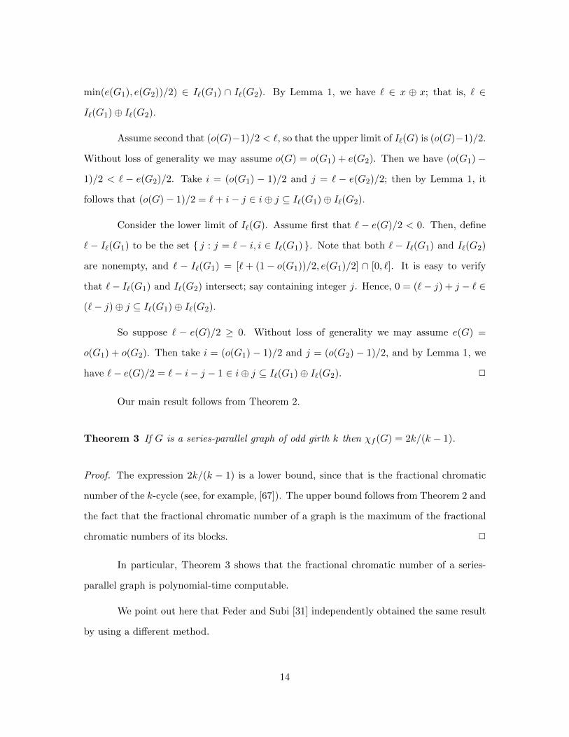
Theorem 3 If G is a series-parallel graph of odd girth k then χf (G) = 2k/(k − 1).

Proof. The expression 2k/(k − 1) is a lower bound, since that is the fractional chromatic

number of the k-cycle (see, for example, [67]). The upper bound follows from Theorem 2 and

the fact that the fractional chromatic number of a graph is the maximum of the fractional

chromatic numbers of its blocks. 2

In particular, Theorem 3 shows that the fractional chromatic number of a series-

parallel graph is polynomial-time computable.

We point out here that Feder and Subi [31] independently obtained the same result

by using a different method.

14

2.3 Defective Colorings

2.3.1 Girth 5

We show below (the probably known fact) that for all d there is a triangle-free series-

parallel graph whose d-defective chromatic number is 3. Indeed, we note in Theorem 7 that

the same is true for fractional chromatic number. However, for girth 5 the situation changes.

We will need the following observation from [6]:

Observation 4 [6] A cyclic series-parallel graph G with girth g contains a path with

b(g − 1)/2c vertices each with degree 2 in G.

Theorem 5 A series-parallel graph G of girth 5 is 1-defective 2-colorable.

Proof. The graph G either contains a vertex of degree 1 (in which case induction is imme-

diate), or is cyclic and therefore by the above observation, contains two adjacent vertices

of degree 2, say x and y. Apply the induction hypothesis to G − {x, y}. Then color x the

opposite color to its neighbor in G− {x, y} and similarly with y. 2

We note that Borodin et al. [6] considered the case where the defect condition is

different for each color. A [d1, . . . , dk]-coloring is a k-coloring of the vertices such that for

each i, the vertices of color i induce a graph of maximum degree at most di. They showed

that a series-parallel graph of girth 7 has a [1, 0]-coloring, and this is best possible; indeed

that for all k there is a series-parallel graph of girth 6 that does not have a [k, 0]-coloring.

2.3.2 Defective Fractional and Circular Colorings

We start with a construction.

Lemma 6 For all d and k ≥ 3, there is a series-parallel graph of odd girth k such that

removing the edges of a subgraph of maximum degree d cannot destroy every k-cycle.

15

Sb(k+2)/4c

Sbk/4cmeans

a copies

Sa

Figure 2.3: A series-parallel graph Gk (k ≥ 5) with given odd girth and large d-defectivefractional chromatic number

Proof. Assume first that k = 3. Construct graph G3 as follows. Start with a complete

bipartite graph K2,d+1 and then for every edge, join its ends by 2d + 1 disjoint paths of

length 2. In our notation, G3 = [((K2 •K2)<2d+1>//K2)<2>]<d+1>. Removal of the edges

of a subgraph of maximum degree d from G3 must leave at least one triangle.

Assume second that k ≥ 5. Let graph Sa = ((K2 •K2)<2d+1>)<a>. (Thus Sa has

diameter 2a.) Then let graph Gk = (Sbk/4c •K2)<d+1>//Sb(k+2)/4c. See Figure 2.3. Clearly

Gk has odd girth k, and removal of the edges of a subgraph of maximum degree d from Gk

must leave at least one k-cycle. 2

From this it follows:

Theorem 7 For all d and k ≥ 3, the maximum d-defective fractional chromatic number of

a series-parallel graph of odd girth k is 2k/(k − 1).

Proof. The upper bound follows from Theorem 3. The lower bound follows from the above

construction. 2

In particular, this theorem shows that for every d there is a series-parallel graph

whose d-defective fractional and circular chromatic numbers are both 3. This gives a neg-

ative answer to Klostermeyer’s question [53] whether every series-parallel graph has a 2-

defective (5, 2)-circular coloring.

The above construction carries over partially to d-defective circular chromatic num-

ber. In particular:

16

Figure 2.4: The graph H1 whose 1-defective circular chromatic number is 8/3

Theorem 8 For all d, the maximum d-defective circular chromatic number of a triangle-

free series-parallel graph is 8/3.

Proof. The upper bound follows from the result of Hell and Zhu (see Theorem 1.1 in [47]).

For the lower bound, let graph Fd = [(K2•K2)<2d+1>•K2]<d+1>//(K2•K2)<2d+1>,

graph Gd = [K2•(K2•K2)<2d+1>]<d+1>//(K2•K2)<2d+1>, and graph Hd = (Fd•Fd)//Gd.

The graph H1 is shown in Figure 2.4. Clearly Hd is triangle-free. It can readily be shown

that if we remove the edges of a subgraph of maximum degree d from Hd, the remaining

graph still contains a copy of the graph of Figure 2.1. Hence Hd has d-defective circular

chromatic number 8/3. 2

The above construction also provides a counterexample to Klostermeyer’s claimed

result [53] that every triangle-free series-parallel graph has a 2-defective (5, 2)-circular col-

oring.

By starting with the graphs constructed by Pan and Zhu [63], one can similarly

show that the maximum d-defective circular chromatic number of a series-parallel graph of

odd girth k is at least the maximum circular chromatic number of a series-parallel graph

of girth k. But there does not seem any reason to believe that the values are equal, since

the question of the maximum circular chromatic number of a series-parallel graph of odd

girth k is unresolved.

17

2.4 Related Questions

Note that simple series-parallel graphs are also the partial 2-trees (see, for exam-

ple, [25]). So it is natural to consider partial k-trees in general. For example, Chlebıkova [18]

showed that: for k ≥ 3, every triangle-free partial k-tree has chromatic number at most k.

So one question is whether this is best possible? Also what happens for fractional/circular

coloring and/or higher girth/odd girth?

18

Chapter 3

Colorings with Fractional Defect

3.1 Introduction

This chapter is based on joint work with Wayne Goddard [39]. As all proofs in the

original paper are provided, we do not give specific references to that paper.

In a proper vertex coloring of a graph, every vertex is assigned one color and that

color is different from each of its neighbors. We consider here a two-fold generalization

of this: a vertex can receive multiple colors and can overlap slightly with each neighbor.

Specifically, each vertex is assigned a fraction of each color, with the total amount of colors

at each vertex summing to 1. The (fractional) defect of a vertex v is defined to be the sum of

the overlaps over all colors and all neighbors of v; the (fractional) defect of the graph is the

maximum of the defects over all vertices. We say that a vertex is monochromatic if it has

only one color, and an edge is monochromatic if both of its endpoints are monochromatic and

they have the same color. Note that if every vertex is monochromatic, then our fractional

defect coincides with the usual definition of defect (see for example [20]).

The idea of assigning vertices multiple colors has been used most notably in frac-

tional colorings (e.g. [64, 57]), but also for example in t-tone colorings [23]. Like in t-tone

colorings (and unlike in fractional colorings), we consider here the situation where one pays

19

for each color used, regardless of how much the color is used. Note that for proper colorings,

allowing one to color a vertex with multiple colors does not yield anything new. For, one

can just choose for each vertex v one color present at v and recolor it entirely that color, and

therefore the minimum number of colors needed is just the chromatic number. Similarly,

with the usual definition of the defect of a vertex as the number of neighbors that share

a color, there is no advantage to using more than one color at a vertex. But we consider

colorings where a vertex overlaps only slightly with each neighbor.

Consider, for example, the Hajos graph. Figure 3.1 gives a 2-coloring of this graph

with defect 4/3 (and this is best possible in that any 2-coloring has at least this much

defect). For another example, consider the complete graph on 3 vertices. Any 2-coloring

of K3 has defect at least 1, but there are multiple optimal colorings: color one vertex red,

one vertex blue, and the third vertex any combination of red and blue.

23 red, 1

3 blue

23 red, 1

3 blue Red

RedBlue

Blue

Figure 3.1: An optimal 2-coloring of the Hajos graph

Our objective is to minimize the defect of the graph. Specifically, for a given number

of colors, what is the minimum defect that can be obtained? If the number of colors is the

chromatic number, then of course there need be no defect. But if the number of colors is

smaller, then there is a defect.

In the rest of the chapter we proceed as follows: in Section 3.2 we introduce notation

and provide elementary results about monochromatic vertices. Thereafter, in Section 3.3,

we consider calculating the parameter in 2-colorings for several graph families, including

fans, wheels, complete multipartite graphs, rooks graphs, and regular graphs. We give exact

values in some cases and bounds in others. We also pose several conjectures. Finally in

20

Section 3.4 we observe that the decision problem is NP-hard.

3.2 Preliminaries

Consider coloring a graph G by using k colors. For color j, let fj(v) be the usage

of color j on vertex v. For each edge vw in G, we call∑k

j=1 min (fj(v), fj(w)) the overlap

between v and w (or alternately, the edge defect of vw).

The defect of vertex v is given by

df (v) =∑

w∈N(v)

k∑j=1

min (fj(v), fj(w)) . (3.1)

In general, the problem is to minimize

maxv

df (v)

over all colorings such that fj(v) is nonnegative and∑k

j=1 fj(v) = 1 for all vertices v. We

denote this minimum by D(G, k), and call it the minimum defect. We call a k-coloring

optimal if it achieves the minimum defect D(G, k).

Note that the existence of the minimum defect is guaranteed, since the objective

function above is continuous and the feasible region is a closed bounded set. Further, the

calculation is at least finite, since, for example, we can prescribe which of fj(v) and fj(w)

are smaller in every min in Equation 3.1 for each vertex v, and thus D(G, k) is the minimum

over exponentially many linear programs.

A related parameter, called the total defect, is∑

v∈V df (v). Note that the total

defect is equal to twice the sum of all edge defects. We define TD(G, k) to be the minimum

of∑

v∈V df (v) over all colorings, and call it the minimum total defect. We prove that there

always exists a coloring that achieves the minimum total defect in which every vertex is

monochromatic:

21

Lemma 9 For graph G and number of colors k, there is a k-coloring that achieves TD(G, k)

in which every vertex is monochromatic.

Proof. Consider any vertex v that is not monochromatic: say f1(v), f2(v) > 0 with f1(v) +

f2(v) = A. Then consider adjusting the coloring such that f1(v) = x and f2(v) = A − x.

As a function of x, the defect of v with any neighbor w is a (piecewise-linear) concave-

down function. Thus, the total defect of the graph, as a function of x, is a concave-down

function, and so its minimum is attained at an endpoint. This means that one can either

replace color 1 by color 2 or replace color 2 by color 1 at v without increasing the total defect.

Repeated application of this replacement yields a coloring with every vertex monochromatic.

2

From the above lemma, it follows that:

Corollary 10 TD(Kn, k) = bn/kc(2n− k − bn/kck).

Proof. By Lemma 9, there is a coloring f that achieves TD(Kn, k) in which every vertex is

monochromatic. Note that the total defect in such a coloring is equal to twice the number

of monochromatic edges. If there exist two color classes whose sizes differ by at least 2, say

there are a1 vertices having color 1, a2 vertices having color 2, and a1 ≥ a2 + 2, then we

recolor one vertex that has color 1 with color 2. Let M denote the increase in the number

of monochromatic edges. We have

(a1 − 1

2

)−(a12

)+

(a2 + 1

2

)−(a22

)= a2 − a1 + 1 < 0.

This contradicts that f achieves minimum total defect. So we may assume that the sizes of

the color classes in f differ by at most 1. Thus there are n−bn/kck color classes having size

bn/kc + 1 and k − n + bn/kck color classes having size bn/kc. For simplicity, let q denote

bn/kc. Then the number of monochromatic edges is

(q

2

)(k − n+ qk) +

(q + 1

2

)(n− qk) = q

(n− (q + 1)k

2

).

22

So TD(Kn, k) = q(2n− k − qk), and the result follows. 2

There are several fundamental results about monochromatic vertices for minimum

defect D(G, k). One is that we may assume that there is a monochromatic vertex of each

color.

Lemma 11 Let k be an integer and G be a graph with at least k vertices. Then there is an

optimal k-coloring of G that has at least one monochromatic vertex for each color.

Proof. Consider any optimal k-coloring, and consider each color j = 1, 2, . . . , k in turn.

Each time, define vertex vj as any vertex other than v1, . . . , vj−1 with the largest usage of

color j; then recolor vj (if needed) such that fj(vj) = 1 and fi(vj) = 0 for all i 6= j. Such a

recoloring does not increase the defect at any vertex. So we will reach an optimal coloring

with the desired property. 2

We next show that the minimum defect is either 0 or at least 1.

Lemma 12 For any graph G and positive integer k, if D(G, k) > 0 then D(G, k) ≥ 1.

Proof. If every vertex is monochromatic, then the defect is an integer and so the result

is immediate. So consider any vertex v that is not monochromatic. If for any color j we

have fj(v) ≥ fj(w) for all neighbors w of v, then we can recolor v to be monochromatically

color j without increasing the defect of any vertex. So we may assume that for every color j

at v, vertex v has a neighbor wj with fj(wj) ≥ fj(v). It follows that

df (v) =∑

w∈N(w)

k∑j=1

min (fj(v), fj(w)) ≥k∑j=1

min (fj(v), fj(wj)) =k∑j=1

fj(v) = 1.

The result follows. 2

It follows from Lemma 12 that the minimum defect in a 2-coloring of a nonbipartite

graph is at least 1. One example of equality is the odd cycle C2n+1: let v1, v2, . . . , v2n+1

23

denote the vertices of C2n+1. Color vi red if i is an odd integer and blue otherwise. That

coloring has defect exactly 1.

Proposition 13 The complete graph Kn has D(Kn, k) = dn/ke − 1.

Proof. This defect is achieved by (inter alia) coloring each vertex with a single color and

using each color as equitably as possible. (This is trivially the best coloring for total defect.)

To see that dn/ke − 1 is best possible, we proceed by induction on n, noting that

the result is trivial if n ≤ k. So assume n > k. By Lemma 11, there is an optimal k-

coloring of Kn that has at least one monochromatic vertex vj for each color 1 ≤ j ≤ k. Let

A = {v1, . . . , vk}. Then the defect of any other vertex w in G equals 1 plus the defect of w

in G − A. By the induction hypothesis, there exists a vertex in G − A that has defect at

least d(n− k)/ke − 1 in G−A. This proves the lower bound. 2

3.3 Two-Colorings of Some Graph Families

We now consider 2-colorings. Unless otherwise specified, we assume the colors are

red and blue, and denote the red usage at vertex v by r(v) (so that the blue usage is 1−r(v)).

3.3.1 Fans

The fan, denoted by Fn, is the graph obtained from a path of order n by adding a

new vertex u and adding an edge between u and every vertex of the path.

Lemma 14 In any 2-coloring of F3 it holds that df (v) + df (w) ≥ 2 where v and w are the

dominating vertices.

Proof. Suppose the dominating vertices are v and w and the other two vertices are a and b.

Let exy denote the overlap min(r(x), r(y))+min(1−r(x), 1−r(y)) between vertices x and y.

24

Then df (v)+df (w) = eva+evb+ewa+ewb+2evw; further, it follows from Corollary 10) that a

triangle has total defect at least 2, and so we have eva+ewa+evw ≥ 1 and evb+ewb+evw ≥ 1.

The result follows. 2

Note that F1 is just K2 and F2 is just K3, and so it holds that D(F1, 2) = 0 and

D(F2, 2) = 1. For the general cases of Fn, we have the following:

Proposition 15 The minimum defect in a 2-coloring of Fn (n ≥ 3) is

D(Fn, 2) =2bn/3cbn/3c+ 1

.

Proof. Let v1v2 . . . vn denote the path of order n, and let u denote the dominating vertex.

We prove the upper bound by the following construction. Set x = 2/(bn/3c + 1).

Let r(u) = 1. Let r(vi) = x if i is a multiple of 3, and 0 otherwise. It can readily be checked

that every vertex vi has defect at most 2 − x, and that vertex u has defect bn/3cx. The

result follows since both these values equal the claimed upper bound.

To prove the lower bound, it suffices to show that D(Fn, 2) ≥ 2n/(n + 3) if n is

a multiple of 3. We partition the path Pn into n/3 copies of P3; thus each P3 along with

vertex u forms a copy of F3. It follows from Lemma 14 that df (u)+∑n/3

i=1 df (v3i−1) ≥ 2n/3,

whence the result. 2

Note that the defect D(Fn, 2) tends to 2 as n increases. The fan is outerplanar.

Several researchers [7, 59] showed that one can ordinarily 2-color an outerplanar graph with

defect at most 2. However, we conjecture that this bound can be improved slightly in the

following sense:

Conjecture 1 D(G, 2) < 2 for any outerplanar graph G.

25

3.3.2 Wheels

The wheel, denoted by Wn, is the graph formed from a cycle of order n by adding a

new vertex and joining it to every vertex of the cycle. The vertex of degree n is called the

hub of the wheel.

Proposition 16 For n ≥ 3, the minimum defect in a 2-coloring of Wn is

D(Wn, 2) =2dn/3edn/3e+ 1

.

Proof. Let x = 2/(dn/3e + 1) and let D be a minimum independent dominating set of

the cycle. For a vertex v on the cycle, let r(v) = x if v ∈ D, and r(v) = 0 otherwise.

Let r(h) = 1 for the hub h. It can readily be checked that every vertex on the cycle has

defect at most 2 − x, and that the hub has defect x|D|. The upper bound follows, since

2− x = x|D| = 2dn/3e/(dn/3e+ 1).

Next we prove the lower bound. When n = 3k, the lower bound follows directly

from Proposition 15. Indeed, D(W3k, 2) ≥ D(F3k, 2) = 2k/(k + 1). So we need to establish

the lower bound for n = 3k + 1 and n = 3k + 2.

Consider an optimal coloring of Wn with hub h and cycle v1, v2, . . . , vn, v1. By

Lemma 11, we may assume there exist vertices u and u′ such that r(u) = 0 and r(u′) = 1.

There are two possible cases.

(a) If h /∈ {u, u′}, then we can form k − 1 edge-disjoint copies of P3 without using

vertex h, u, or u′. Let S denote the set of centers of these copies. By Lemma 14, it follows

that the total defect of S ∪ {h} within these copies is at least 2(k − 1). Further, vertices u

and u′ together contribute defect 1 to the hub h. It follows that, in the graph as a whole,

df (h) +∑

s∈S df (s) ≥ 2k − 1, and so G has defect at least (2k − 1)/k. If k ≥ 2, then

(2k − 1)/k ≥ (2k + 2)/(k + 2), and we are done.

So consider the case when k = 1. Assume first that n = 5. Suppose u and u′ are

consecutive on the cycle; say u = v1 and u′ = v2. Then G− {u, u′} is a copy of F3. Since u

26

and u′ together contribute defect 1 to h, it follows from Lemma 14 that df (h) + df (v4) ≥ 3,

and so G has defect at least 3/2. So assume without loss of generality that u = v1 and

u′ = v3. If h has two neighbors that are at least as red as h, and two other neighbors that

are at most as red as h, then h has defect at least 2. So, without loss of generality, we

may assume that r(v2), r(v4), r(v5) ≤ r(h). Then, the defect that h receives from {v2, v5}

is 2− 2r(h) + r(v2) + r(v5), and the defect that u receives from {v2, v5} is 2− r(v2)− r(v5).

That is, the sum of the defects that h and u receive from {v2, v5} is at least 2. Since h also

receives defect 1 from u and u′, it follows that df (u) + df (h) ≥ 3, and the result follows.

The argument for n = 4 is similar and omitted.

(b) If h ∈ {u, u′}, then, without loss of generality, we may assume that u = v1 and

u′ = h. Note that vn receives defect 1 from {v1, h}. Let index j be such that vj is the

redder vertex of vn−1 and vn. Then vn−1 and vn have at least 1− r(vj) of blue overlap and

so df (vn) ≥ 2− r(vj).

Further, one can form k edge-disjoint copies of P3 without using vertex h or vj .

Let S denote the set of centers of these copies. By Lemma 14 and noting that the hub h

receives defect r(vj) from vertex vj , it follows that df (h) +∑

s∈S df (s) ≥ 2k + r(vj).

Thus df (h) + df (vn) +∑

s∈S df (s) ≥ 2k + 2, and the result follows. 2

3.3.3 Complete multipartite graphs and compositions

We consider here complete multipartite graphs. These can be thought of as taking

a complete graph and replacing each vertex by an independent set with the same adjacency.

In general, we define G[aK1] to be the composition of G with the empty graph on a vertices;

that is, the graph obtained by replacing every vertex v of G with a vertex set Iv of size a

such that a vertex of Iv is adjacent to a vertex of Iw if and only if v and w are adjacent

in G.

There are two simple bounds:

27

Proposition 17 For any graph G,

(a) TD(G[aK1], k) ≥ a2 TD(G, k).

(b) D(G[aK1], k) ≤ aD(G, k).

Proof. (a) Let n denote the order of G. Consider a k-coloring of G[aK1] that achieves

TD(G[aK1], k). Note that G[aK1] contains an copies of G (by choosing one vertex from

each set Iv of size a). The sum of the total defects of those an graphs is at least an TD(G, k).

Since each edge of G[aK1] is contained in exactly an−2 of those graphs, the result follows

by averaging.

(b) Take an optimal coloring of G and replicate it. 2

We let K(m)a denote the complete m-partite graph with a vertices in each partite

set; that is K(m)a = Km[aK1]. It follows that:

Proposition 18 If m is a multiple of k, then the complete multipartite graph K(m)a can be

k-colored with defect (m/k − 1)a, and this is best possible.

But if m is not a multiple of k, the result is not clear. We have the following

conjecture:

Conjecture 2 The minimum defect in a k-coloring of K(m)a is (dm/ke − 1)a.

In fact, we do not have an example that precludes it being the case that it always

holds that D(G[aK1], k) = aD(G, k).

We shall prove Conjecture 2 for 2 colors. We need the following definitions. Define

a vertex x as large if r(x) > 1/2 and small if r(x) < 1/2. Also we let N(x) denote the set

of neighbors of x, U(x) denote the set of vertices y in N(x) with r(y) ≥ r(x), and L(x)

denote the set of vertices y in N(x) with r(y) < r(x).

We also need the following observations and lemmas. Some of them are very easy

to verify and so the proofs are omitted:

28

Observation 19 If r(x) = 1/2, then df (x) ≥ |N(x)|/2.

Observation 20 If two vertices are both large (or both small), then the overlap between

them is greater than 1/2.

Observation 21 df (x) ≥ min (|U(x)|, |L(x)|).

Lemma 22 df (x) ≥ |N(x)|/2 if either

(a) x is large and |U(x)| ≥ |L(x)|,

or (b) x is small and |U(x)| ≤ |L(x)|.

Proof. It suffices to prove it for the case that x is large. We pair each vertex in L(x) with a

vertex in U(x). Then each pair contributes at least 1 to df (x). By Observation 20, each of

the remaining vertices in U(x) contributes more than 1/2 to df (x). Hence df (x) ≥ |N(x)|/2.

2

Lemma 23 If x is large and y is small, then max (df (x), df (y)) ≥ |N(x) ∩N(y)|/2.

Proof. If |U(x)| ≥ |L(x)|, then we have df (x) ≥ |N(x)|/2 ≥ |N(x)∩N(y)|/2 by Lemma 22.

So we may assume |U(x)| < |L(x)|. Similarly we may assume |U(y)| > |L(y)|. Note that we

can increase r(x) to 1 and decrease r(y) to 0 without increasing the defect of either vertex.

It follows that df (x) + df (y) is at least their common degree, whence the result. 2

Lemma 24 If all neighbors of x are large (small), then r(x) can be changed to 0 (1) without

increasing the defect of any vertex.

Proof. It suffices to prove it for the case that all neighbors of x are large. Let v be any

neighbor of x. The overlap between them is 1− |r(v)− r(x)|. If r(x) is changed to 0, then

the overlap becomes 1 − r(v). Since r(v) > 1/2, we have 1 − |r(v) − r(x)| ≥ 1 − r(v) and

the conclusion follows. 2

29

Proposition 25 The minimum defect in a 2-coloring of K(m)a is (dm/2e − 1)a.

Proof. Such defect is attained by coloring all vertices in bm/2c of the partite sets with red,

and the remaining vertices blue. So we need to prove that this is best possible.

If m is even, Proposition 17 shows that TD(K(m)a , 2) ≥ m(m/2 − 1)a2, and thus

some vertex has defect at least (m/2− 1)a. So assume m is odd.

If there is a vertex v in the graph with r(v) = 1/2, then df (v) ≥ (m − 1)a/2 =

(dm/2e − 1)a by Observation 19. Also, if there is a partite set that contains both a large

vertex and a small vertex, then the result follows from Lemma 23.

Hence, we may assume every partite set contains either only large vertices or only

small vertices. Without loss of generality, assume at least (m + 1)/2 partite sets contain

only large vertices. Let x be the large vertex with minimum r(x). Note that |U(x)| ≥

(m− 1)a/2 ≥ |L(x)|, and therefore df (x) ≥ (m− 1)a/2 = (dm/2e − 1)a by Lemma 22. 2

Proposition 26 The minimum defect in a 2-coloring of the complete tripartite graph Ka,b,c

with a ≤ b ≤ c is bc/(b+ c− a).

Proof. Let A, B, and C denote the partite sets of order a, b, and c, respectively. The

upper bound is attained by coloring all vertices v in A with r(v) = 0, all vertices in C with

r(v) = 1, and all vertices in B with r(v) = x, where x is chosen to give the vertices in A

and B the same defect, namely x = (b− a)/(b+ c− a).

Now we prove the lower bound. Let x1, x2, . . . , xa be the vertices in A with r(x1) ≤

r(x2) ≤ . . . ≤ r(xa), y1, y2, . . . , yb be the vertices in B with r(y1) ≤ r(y2) ≤ . . . ≤ r(yb), and

z1, z2, . . . , zc be the vertices in C with r(z1) ≤ r(z2) ≤ . . . ≤ r(zc).

Case 1: a ≤ b ≤ c ≤ a+ b.

Then we have (b + c)/2 ≥ (a + c)/2 ≥ (a + b)/2 ≥ bc/(b + c − a). If there is a

vertex v in the graph with r(v) = 1/2, then the conclusion follows from Observation 19.

30

Also, if there is a partite set that contains both a large vertex and a small vertex, then the

conclusion follows from Lemma 23. Hence we may assume every partite set contains either

only large vertices or only small vertices, and by symmetry we only need to consider the

following four cases:

Case 1.1: all vertices in the graph are large.

By Observation 20, we have df (xi) ≥ (b+c)/2 for every 1 ≤ i ≤ a. So the conclusion

follows.

Case 1.2: all vertices in A are small and all the other vertices are large.

Let u be the large vertex with minimum r(u). By Lemma 22, df (u) ≥ (a + b)/2

and the conclusion follows.

Case 1.3: all vertices in B are small and all the other vertices are large.

By Lemma 24, we may assume r(yj) = 0 for every 1 ≤ j ≤ b. If r(x1) ≤ r(z1), then

by Lemma 22, df (x1) ≥ (b+ c)/2. So assume r(x1) > r(z1). We have

df (xa) = b(1− r(xa)) +c∑

k=1

(1− |r(xa)− r(zk)|)

≥ b(1− r(xa)) +c∑

k=1

(r(xa) + r(zk)− 1)

= (b− c)(1− r(xa)) +

c∑k=1

r(zk)

≥ (b− c)(1− r(xa)) + c r(z1),

and

df (z1) =

a∑i=1

(1− (r(xi)− r(z1))) + b(1− r(z1))

=a∑i=1

(1− r(xi)) + (a− b)r(z1) + b

≥ a(1− r(xa)) + (a− b)r(z1) + b.

31

Hence, (b−a) df (xa) + c df (z1) ≥ [(b−a)(b− c) +ac](1− r(xa)) + bc ≥ bc. It follows

that max (df (xa), df (z1)) ≥ bc/(b+ c− a).

Case 1.4: all vertices in C are small and all the other vertices are large.

By Lemma 24, we may assume r(zk) = 0 for every 1 ≤ k ≤ c. If r(x1) ≤ r(y1), then

we have

df (x1) = c(1− r(x1)) +

b∑j=1

(1− (r(yj)− r(x1)))

= c+ (b− c)r(x1) +

b∑j=1

(1− r(yj))

≥ c+ (b− c)r(x1),

and

df (y1) =

a∑i=1

(1− |r(xi)− r(y1)|) + c(1− r(y1))

≥a∑i=1

(r(xi) + r(y1)− 1) + c(1− r(y1))

= (c− a)(1− r(y1)) +

a∑i=1

r(xi)

≥a∑i=1

r(xi)

≥ a r(x1).

Hence, b df (x1) + (c−a) df (y1) ≥ bc+ [b(b− c) + (c−a)a]r(x1) = bc+ (b+a− c)(b−

a)r(x1) ≥ bc. It follows that max (df (x1), df (y1)) ≥ bc/(b+ c− a).

Similarly, if r(x1) > r(y1), then it can be verified that

df (x1) ≥ (c− b)(1− x1) +b∑

j=1

r(yj) ≥ b r(y1),

32

and

df (y1) =a∑i=1

(1− r(xi)) + c+ (a− c)r(y1) ≥ c+ (a− c)r(y1).

Hence, (c− a) df (x1) + b df (y1) ≥ bc. It follows that max (df (x1), df (y1)) ≥ bc/(b+

c− a).

Case 2: a ≤ b < a+ b < c.

Then we have (b+ c)/2 ≥ (a+ c)/2 > c/2 > bc/(b+ c− a). By Observation 19 and

Lemma 23, we only consider the case that the vertices of A ∪ B are either all large or all

small. Without loss of generality, assume they are all large. Then by Lemma 24, we may

assume r(zk) = 0 for every 1 ≤ k ≤ c.

If r(x1) ≤ r(y1), then df (x1) ≥ b by Observation 21. So assume r(x1) > r(y1). But

then by the same argument as that in Case 1.4, we have max (df (x1), df (y1)) ≥ bc/(b+c−a).

2

For another composition, consider Cm[aK1] where m is odd. We now prove that

D(Cm[2K1], 2) = 2. There are at least two different optimal colorings. The first such

coloring is obtained by taking an optimal coloring for Cm and replicating it. The second

such coloring is obtained by, for each copy of 2K1, coloring one vertex red and one vertex

blue.

Proposition 27 For m odd, D(Cm[2K1], 2) = 2.

Proof. Consider a 2-coloring of Cm[2K1]. We need to show that the defect is at least 2.

As in the proof of Proposition 25, we may assume that every copy of 2K1 contains either

two large vertices or two small vertices. Since m is odd, it follows that there must be two

adjacent copies of the same type. Without loss of generality, assume u1 and u2 are adjacent

to v1 and v2 with all four vertices being large. If any x ∈ {u1, u2, v1, v2} has |U(x)| ≥ 2,

then the lower bound follows from Lemma 22(a). Therefore we may assume that |U(x)| ≤ 1

33

for every x ∈ {u1, u2, v1, v2}. This means that each ui is redder than some vj and vice versa,

a contradiction. 2

3.3.4 Rooks graphs and Cartesian products

Recall that the Cartesian product G2H is the graph whose vertex set is V (G) ×

V (H), in which two vertices (u1, u2) and (v1, v2) are adjacent if u1v1 ∈ E(G) and u2 = v2,

or u1 = v1 and u2v2 ∈ E(H).

We will need the obvious lower bound for the total defect of Cartesian products.

Proposition 28 Let G and H be graphs of order m and n respectively. Then

TD(G2H, k) ≥ mTD(H, k) + nTD(G, k).

Proof. The defect of a vertex in the product is the sum of the defects in its copies of G

and H. 2

Recall that rooks graphs are the Cartesian product of complete graphs. We denote

the vertices of Km2Kn by (i, j) with 1 ≤ i ≤ m, 1 ≤ j ≤ n.

Lemma 29 The rooks graph Km2Kn can be 2-colored with defect dm/2e+ dn/2e − 2.

Proof. Color vertex (i, j) red if i and j have the same parity and blue otherwise. 2

Corollary 30 Let m and n be even integers. Then D(Km2Kn, 2) = m/2 + n/2− 2.

Proof. The upper bound follows from Lemma 29. The lower bound follows from Proposi-

tion 28, since TD(Ks, 2) = s(s/2−1) for s even (Corollary 10), and thus TD(Km2Kn, 2) ≥

mn(n/2− 1) + nm(m/2− 1). 2

We show below that the upper bound in Lemma 29 is not always optimal. In fact

we conjecture that it is never optimal when m and n are both odd, except for the case that

m = n = 3.

34

Lemma 31 D(K32K3, 2) = 2.

Proof. The upper bound is from Lemma 29.

We have two proofs of the lower bound, one by computer and one by hand. Both

proofs entail converting the question to a set of linear programs.

Observe that given a coloring, one can generate an acyclic orientation by orienting

each edge from smaller to larger proportion of red (with ties broken by vertex number).

Further, if N1 is the set of neighbors of vertex v with more red and N2 is the set of

neighbors of v with less red, then Equation 3.1 simplifies to

df (v) = |N1|r(v) + |N2|b(v) +∑w∈N2

r(w) +∑w∈N1

b(w),

where b(x) = 1− r(x).

We continue by enumerating the acyclic orientations. For each such orientation, we

add the constraints that r(u) ≤ r(v) for all arcs uv. That is, minimizing the defect for a

given orientation is a linear program.

Further, if any vertex has in- and out-degree 2 for the orientation, the defect is

definitely at least 2 (by Observation 21). With several pages of calculation or by using a

computer, one can show that K32K3 has eight acyclic orientations (up to symmetry) that

need to be considered, and then solve the eight associated linear programs. We omit the

details. 2

In contrast, we found a coloring of K32K5 that beats the bound of Lemma 29:

Lemma 32 D(K32K5, 2) ≤ 38/13.

Proof. A 2-coloring of K32K5 is shown in the matrix below. The element (i, j) of the

matrix is the red-usage on vertex (i, j).

35

0 8/13 0

0 0 8/13

1 11/13 0

1 0 11/13

6/13 1 1

It can be verified that the defect of the coloring is 38/13. 2

The above coloring can be extended to show that Lemma 29 is not optimal for m = 3

and n odd, n ≥ 5, and indeed that D(K32Kn, 2) ≤ n/2 + 11/26 in this case. However,

this is still not best possible. For example, one can get defect 42/11 for K32K7 and defect

14/3 for K32K9 by the colorings illustrated in the matrices below:

1 0 1

4/11 1 1

0 8/11 0

1 1 4/11

1/11 0 1

0 8/11 0

1 0 1/11

2/3 0 0

0 2/3 0

0 0 2/3

0 1 1

0 1 1

1 0 1

1 0 1

1 1 0

1 1 0

We used simulated annealing computer search (that is, a randomized search for a

coloring) to find upper bounds. Though we have no exact values, it seems to us that the

search results suggest the following:

Conjecture 3 (a) If m+ n is odd, then D(Km2Kn, 2) = (m+ n− 3)/2.

(b) If mn is odd and greater than 9, then D(Km2Kn, 2) < dm/2e+ dn/2e − 2.

36

Note that Conjecture 3 (a) is trivially true for the case that m = 2 (or n = 2), since

D(K22Kn, 2) ≥ D(Kn, 2) = (n− 1)/2.

Proposition 28 yields the following lower bounds:

Corollary 33

(a) If both m and n are odd, D(Km2Kn, 2) ≥ (m+ n)/2− 2 + 1/(2m) + 1/(2n).

(b) If m is even and n is odd, D(Km2Kn, 2) ≥ (m+ n)/2− 2 + 1/(2n).

For more colors we have the trivial observation that D(Kn2G, k) = dn/ke − 1 for

any k-partite graph G, as a corollary of Proposition 13.

3.3.5 Regular graphs

Lovasz [58] showed that we can ordinarily 2-color a cubic graph with defect at

most 1. Therefore D(G, 2) = 1 for all nonbipartite cubic graphs G.

For a 4-regular graph, Lovasz’s result shows that one can ordinarily 2-color it with

defect at most 2. We conjecture that this can be improved. Proposition 27 shows that the

composition G = Cm[2K1] where m is odd has D(G, 2) = 2. Using simulated annealing,

the computer can find a 2-coloring with defect smaller than 2 for all 4-regular graphs on

up to 14 vertices, except for the compositions of odd cycles, and the two graphs K5 and

K32K3, which we saw earlier have minimum defect 2. We give a conjecture for the general

behavior:

Conjecture 4 Apart from G = Cm[2K1] where m is odd, it holds that D(G) < 2 for all

but finitely many connected 4-regular graphs.

3.4 Complexity

Unsurprisingly, it is NP-hard to determine if there is a coloring with defect at most

some specified d.

37

One way to see this is that fractional defect 2-coloring is NP-hard even for d = 1.

One can extend Lemma 11 to show that in graphs of minimum degree at least 3, a 2-coloring

with defect 1 can only be a coloring with monochromatic vertices. Thus the fractional defect

2-coloring problem is equivalent to the ordinary defective 2-coloring problem in such graphs.

The latter problem was shown to be NP-hard by Cowen [22]. (Actually, we need ordinary

1-defect coloring to be NP-hard in graphs with minimum degree at least 3. But one can

transform a graph to having minimum degree at least 3 without changing the coloring

property by adding, for each vertex v, a copy of K4 and joining v to one vertex of the K4.)

38

Chapter 4

Vertex Colorings without Rainbow

Subgraphs

4.1 Introduction

This chapter is based on joint work with Wayne Goddard [41]. As all proofs in the

original paper are provided, we do not give specific references to that paper.

Given a (not necessarily proper) vertex coloring of a graph G, recall that a subgraph

is rainbow if all its vertices receive distinct colors and monochromatic if all its vertices receive

the same color. For a graph F , we refer to a (not necessarily proper) vertex coloring of G

without rainbow subgraphs isomorphic to F as a no-rainbow-F coloring of G (valid coloring

for short); we define the F -upper chromatic number of G as the maximum number of colors

that can be used in a valid coloring. We denote this maximum by NRF (G). A valid coloring

is optimal if it uses exactly NRF (G) colors.

There are many papers on the edge-coloring version, where the parameter is called

the anti-Ramsey number. Note that this parameter is also exactly 1 less than the rainbow

number, which is the minimum number of colors such that every edge-coloring of G with

at least that many colors produces a rainbow F . For the edge-coloring case, the most

39

studied situation is when G is complete and F is a cycle, clique, tree, or matching. For

example, a Gallai-coloring is an edge-coloring of the complete graph without a rainbow

triangle [44, 43]. For a survey of anti-Ramsey theory, see [33].

In contrast, not much has been written about the vertex-coloring case. There are

two papers on avoiding rainbow induced subgraphs: [3] and [52]. More recently, the special

case where F is P3 was considered by Bujtas et al. [10] (under the name 3-consecutive upper

chromatic number), and then the case where F is K1,k was considered by Bujtas et al. [9]

(under the name star-[k] upper chromatic number). Besides these, a related question that

has been studied is coloring embedded graphs with no rainbow faces, see for example [24, 65].

Graph colorings without rainbow (monochromatic) subgraphs fall within the theory

of mixed hypergraphs introduced by Voloshin (see, for example, [74]; see [75] for an overview

of the theory, and see [71] for a survey of results and open problems).

In general, a mixed hypergraph H is a triple (X, C,D), where X is the vertex set, and

C and D are families of subsets of X, called the C-edges and D-edges, respectively. A proper

coloring of H is an assignment of one color to each vertex in X such that each C-edge has

at least two vertices with a Common color, and each D-edge has at least two vertices with

Distinct colors. The case that C is an empty set is just the proper coloring of hypergraphs;

while the case that D is an empty set leads to the notion called C-coloring (see [12]).

Note that the theory of mixed hypergraphs provides a general framework for graph

colorings without rainbow (monochromatic) subgraphs: say we color a graph G with vertex

set V forbidding monochromatic subgraph M and rainbow subgraph R, then consider the

mixed hypergraph H = (X, C,D) where X = V , C consists of the vertex subsets of cardi-

nality |V (R)| which induces a subgraph containing R in G, and D consists of the vertex

subsets of cardinality |V (M)| which induces a subgraph containing M in G. One can see

that there is a bijection between the colorings of G and the proper colorings of H.

In this chapter, we investigate the F -upper chromatic number for certain graph

classes. We proceed as follows: in Section 4.2 we present some basic observations. Then in

40

Section 4.3 we consider the case that F is a path on three vertices, in Section 4.4 the case

that F is a triangle, and in Section 4.5 the case that F is the star K1,r.

4.2 Preliminaries

Bujtas et al. [9] observed the following when F is a star, but the results hold in

general:

• For fixed F , the parameter is monotonic: if H is a spanning subgraph of G, then

NRF (G) ≤ NRF (H).

• If F is connected and G is disconnected, then NRF (G) is the sum of the NRF ’s of the

components of G.

• The chromatic spectrum has no gaps: G has a coloring without a rainbow F using k

colors for 1 ≤ k ≤ NRF (G). Simply take an optimal coloring and successively merge

color classes.

• NRF (G) = |V (G)| if and only if G is F -free.

• NRF (G) ≥ |F | − 1, provided G has that many vertices.

For a natural lower bound, one can define an F -bi-cover of a graph as a set of vertices

that contains at least two vertices from every copy of F . It follows that one can obtain a

no-rainbow-F coloring by giving all vertices in an F -bi-cover the same color and giving all

other vertices unique colors. For example, if G is a connected graph of order at least 3, then

a P3-bi-cover is the complement of a packing. (A packing is a set of vertices at pairwise

distance at least 3; the packing number ρ(G) is the maximum size of a packing.) The lower

bound NRP3(G) ≥ ρ(G) + 1 follows. A vertex cover is an F -bi-cover for any connected

non-star graph F . In this case we have NRF (G) ≥ α(G) + 1 (where α(G) denotes the

independence number) provided G is not empty.

41

We say that a set S bi-covers a subgraph H if at least two vertices of H are in S.

For positive integer s, define bF (s) to be the maximum number of copies of F that can be

bi-covered by using a set of size s. Note that bF (1) = 0.

Proposition 34 Suppose that graph G of order n contains f copies of F and that bF (s) ≤

a(s− 1) for all s. Then NRF (G) ≤ n− f/a.

Proof. Consider a no-rainbow-F coloring. Say one uses k colors, being used s1, . . . , sk times

respectively. Then k = n −∑k

i=1(si − 1). Since every copy of F has to be bi-covered by

some color class,∑k

i=1 bF (si) ≥ f . It follows that k ≤ n− f/a. 2

4.3 Forbidden P3

The parameter NRP3(G) can also be thought of as the maximum number of colors

in a coloring such that each vertex sees at most one color other than its own.

4.3.1 Fundamentals

There are two natural lower bounds.

Proposition 35

(a) For a graph G, NRP3(G) ≥ diam(G)/2 + 1.

(b) For any nonempty graph G, NRP3(G) ≥ ρ(G) + 1.

Proof. (a) Let x be a vertex of eccentricity diam(G), and color each vertex v by dd(x, v)/2e,

where d(x, v) denotes the distance from x to v.

(b) See the previous section. (Give every vertex in a maximum packing a unique

color, and give all other vertices the same color.) 2

Bujtas et al. [10] showed a partial converse to the first lower bound:

42

Proposition 36 [10] If G has diameter 2, then NRP3(G) = 2.

For example, rooks graphs have diameter 2 and so they have P3-upper chromatic

number 2.

Bujtas et al. [10] showed that the P3-upper chromatic number of a connected graph

is at most one more than its vertex cover number:

Theorem 37 [10] For every connected graph G, it holds that NRP3(G) ≤ β(G) + 1.

Bujtas et al. [10] also showed that for every tree T , NRP3(T ) is one more than the

matching number of T :

Theorem 38 [10] For every tree T , it holds that NRP3(T ) = m(T ) + 1.

From the above theorem, we obtain the following upper bound for NRP3(G):

Corollary 39 For a connected graph G of order n, NRP3(G) ≤ bn/2c+ 1.

Proof. Let T be a spanning tree of G. By theorem 38, NRP3(T ) = m(T ) + 1 ≤ bn/2c+ 1.

Since NRP3(G) ≤ NRP3(T ), the result follows. 2

It is natural to ask what graphs achieve equality in Corollary 39.

The corona cor(G) of a graph G is the graph obtained from G by adding, for each

vertex v in G, a new vertex v′ and the edge vv′. The new vertices are called the leaves of

the corona. Note that coronas achieve equality in Corollary 39:

Observation 40 If G is connected, then NRP3(cor(G)) = |G|+ 1.

Proof. The lower bound follows from Proposition 35(b). That is, give all the leaves unique

colors and give all the original vertices of G the same color. The upper bound is from

Corollary 39. 2

43

Note that in an optimal no-rainbow-P3 coloring of a graph, the subgraphs that are

induced by the color classes do not have to be connected. For example, Figure 4.1 shows

a graph G with NRP3(G) = 4, which is uniquely attained by giving each white vertex a

unique color and all black vertices the same color.

Figure 4.1: A graph whose optimal no-rainbow-P3 coloring has a disconnected color class

4.3.2 Complexity

We next show that calculating NRP3(G) is NP-hard. We will need the following

construction: for graph G, define graph M(G) by adding, for every vertex v in G, a new

vertex v′ adjacent to v, and adding edges to make C = { v′ : v ∈ V (G) } a clique.

Observation 41 For any nontrivial graph G it holds that NRP3(M(G)) = ρ(G) + 1.

Proof. Note that ρ(M(G)) = ρ(G). So the lower bound follows from Proposition 35(b). To

prove the upper bound, consider a coloring of M(G) with no rainbow P3. Note that the

clique C contains at most two colors. There are two cases.

First, consider that C contains two colors. Note that for every vertex v in V (G),

there is a vertex w′ such that v′ and w′ receive different colors. It follows that v receives

one of the two colors in C. That is, the coloring uses two colors.

Second, consider that C contains only one color, say red. Let v and w be vertices of

V (G) such that neither is red and they have different colors. Then they cannot be adjacent,

since that would make vww′ rainbow, nor can they have a common neighbor x, since x

would see three colors. It follows that if we take one vertex of each non-red color, we obtain

a packing. That is, the number of non-red colors is at most ρ(G), as required. 2

44

As a consequence it follows that computing NRP3(G) is NP-hard, since computing

the packing number is NP-hard [14].

In contrast, Bujtas et al. [10] showed that determining whether a graph G has

NRP3(G) = 3 or NRP3(G) = 4 is solvable in polynomial time.

4.3.3 Graph Families and Operations

4.3.3.1 Clones

In general, if v and w have the same neighbors (themselves excluded), then NRF (G) ≥

NRF (G− v), since one can take any coloring of G− v and give v the same color as w. But

we have equality for F = P3:

Observation 42 Assume vertices v and w are such that N(v) − {w} = N(w) − {v} 6= ∅.

Then NRP3(G) = NRP3(G− v).

Proof. Consider a valid coloring of G. Let x be any common neighbor of v and w. If v

and w have different colors, then x must have the same color as one of them. If x has the

same color as v, then the coloring restricted to G − v is a valid coloring with every color

of G. If x has the same color as w, then the coloring restricted to G−w is a valid coloring

with every color of G. Note that G− w = G− v and so the conclusion follows. 2

4.3.3.2 Maximal Outerplanar Graphs

We now consider avoiding rainbow P3 in maximal outerplanar graphs. The minimum

value of NRP3(G) for an outerplanar graph of order n is obtained by the fan (having value 2).

The maximum value for a maximal outerplanar graph of order n is given by the following:

Theorem 43 The maximum value of NRP3(G) for a maximal outerplanar graph G of order

n ≥ 3 is bn/3c+ 1.

45

Proof. We prove the lower bound by the following construction: start with a cycle v1v2 . . . vnv1.

For 1 ≤ i ≤ bn/3c, assign v3i a distinct color. Then use one additional color for all the

remaining vertices, and add edges between them until we have a maximal outerplanar

graph G. Clearly, exactly bn/3c+ 1 colors are used and there is no rainbow P3.

We prove the upper bound by induction on n. It suffices to show that NRP3(G) ≤

n/3 + 1. It is easy to verify the result for n = 3. For larger n, the outer cycle of G has a

chord.

The first case is that there is a chord, say uv, with different colors on its ends. Let

V1 and V2 be the vertex sets of the components of G−{u, v}. Let Gi be the subgraph of G

induced by the vertices Vi ∪ {u, v}. Note that Gi is a maximal outerplanar graph. By the

induction hypothesis, Gi has at most |Gi|/3 + 1 colors. But G1 and G2 share two colors. So

the total number of colors in G is at most (|V1|+2)/3+1+(|V2|+2)/3+1−2 = (n+2)/3 <

n/3 + 1.

The second case is that every chord is monochromatic. Since the chords induce a

connected subgraph of G, it follows that all the vertices with degree at least 3 in G have

the same color, say red. Let X be the set consisting of one vertex of each remaining color.

Since the vertices with degree 2 are independent, it follows that X is independent.

Further, vertices x1 and x2 of X cannot have a common neighbor, since that vertex would

be red and we would have a rainbow P3. It follows that |X| ≤ ρ(Cn) ≤ bn/3c, and so the

colors in G is at most bn/3c+ 1. 2

Note that there are maximal outerplanar graphs where NRP3(G) > ρ(G) + 1.

4.3.3.3 Cubic Graphs

We consider now avoiding rainbow P3 in cubic graphs. It is unclear what the mini-

mum and maximum values of NRP3(G) (for cubic graphs G of fixed order) are. Some data

generated by a computer search is shown in Table 4.1:

46

order 4 6 8 10 12 14 16 18

min 2 2 2 2 3 3 4 4max 2 2 3 4 4 5 6 7

Table 4.1: Extremal values of NRP3(G) for cubic graphs G of fixed order

Computer search shows that, for n ≤ 18, the minimum value of the parameter is

one more than the minimum value of the packing number. However, it is unclear what the

asymptotics of the packing number are. Favaron [30] showed that ρ(G) ≥ n/8 for a cubic

graph G of order n other than the Petersen graph, but it is unclear if this bound is sharp in

general. Furthermore, it is unclear under what circumstances a graph has parameter equal

to the packing number lower bound.

We consider next the maximum value of the parameter for cubic graphs of order n.

Theorem 44 For any connected cubic graph G on n ≥ 6 vertices, NRP3(G) ≤ 2n/5.

Proof. We extend a counting idea suggested in [9]. For a color c, define CN(c) as the number

of closed neighborhoods that c is in. (Equivalently, the number of vertices dominated by

a vertex of color c.) Let A =∑

c CN(c); that is, A is the number of pairs (c, v) where c

is a color that occurs in N [v]. The requirement of no rainbow P3 means that each closed

neighborhood has at most 2 colors in it, and so A ≤ 2n. To prove the theorem, it suffices

to show that the average value of CN(c) is at least 5.

Since G is cubic, it is immediate that CN(c) ≥ 4 for all colors c. Call a color c

sparse if CN(c) = 4. Say vertex v has color c. Then all other vertices with color c, if any,

must be neighbors u of v such that N [u] = N [v]. Since the graph is not K4, it follows that

there are at most two vertices with color c. The remaining neighbors of v (which are also

the neighbors of the other vertex of color c, if any) must be the same color, say c′.

We claim that CN(c′) ≥ 6. By connectivity there is a vertex w that is not in N [v]

but has a neighbor x in N [v]. Since N [w] does not contain color c but vxw is a P3, it

follows that x and w are both color c′. Since n ≥ 6, there must be a vertex that is not

47

in N [v] ∪ {w} and is adjacent to a vertex of color c′ in N [v] ∪ {w}. So CN(c′) ≥ 6. In

particular, CN(c) + CN(c′) ≥ 10.

Now, suppose that the same color surrounds multiple sparse colors. Say, we have

c1, . . . , cb such that c′1 = . . . c′b = d. Then we claim that CN(d) ≥ 4b. This follows by noting

that the N [vi] are disjoint if vi has color ci, and all of N [vi] is dominated by a vertex of

color d. It follows that CN(d) +∑

i CN(ci) ≥ 8b ≥ 5(b+ 1), since b ≥ 2.

So, by partitioning the sparse colors into sets based on the surrounding color, it

follows that the average value of CN(c) is at least 5, whence the result. 2

The computer data verifies that the maximum value is b2n/5c for 6 ≤ n ≤ 18.

However, the bound in Theorem 44 might not be sharp in general. Let H be the graph of

order 5 obtained from K4 by subdividing one edge. Let I0 be built from two copies of H by

adding an edge joining the vertices of degree 2. Computer search confirms that for n = 10

this is the unique graph that achieves the maximum value. In general, let graph Ij be the

cubic graph built from two copies of H by adding j copies of K4 − e between the copies

of H. For n = 14, the graph I1 is a graph that achieves the maximum value. For n = 18,

the graph I2 is a graph that achieves the maximum value. But there is one other graph

that achieves the maximum value: take three copies of H and one copy of K3 and add

edges to make a connected cubic graph. See Figure 4.2. It can be checked that NRP3(Ij) is

3n/8 +O(1). It is unclear if this is best possible.

4.4 Forbidden Triangles

We consider now colorings that forbid a rainbow copy of the other connected graph

on three vertices, a triangle. That is, we consider colorings where every triangle has a

monochromatic edge.

We saw earlier that NRK3(G) ≥ α(G) + 1, provided G is nonempty. In particular,

we note that if every edge of the graph is in a triangle, then a subset S is a K3-bi-cover if

48

Figure 4.2: The two cubic graphs of order 18 with maximum NRP3

and only if S is a vertex cover. Note that when F is a complete graph, every color class in

an optimal no-rainbow-F coloring of a graph must induce a connected subgraph. (Assume

to the contrary that color red induces a disconnected subgraph; then change the vertices in

one red component to a new color pink. There cannot be a red vertex and a pink vertex

together in a clique, since the pink vertex and red vertex were not adjacent.)

One can again investigate the minimum and maximum values of the parameter for

graphs of fixed order in particular classes. For example, the extremal values of NRK3(G)

for cubic graphs G of order n are straightforward. The maximum is n, achieved by a

triangle-free graph. The minimum is 2n/3, achieved by a cubic graph with n/3 disjoint

triangles.

4.4.1 Maximal Outerplanar Graphs

We show that the value of NRK3(G) for a maximal outerplanar graph G of fixed

order does not depend on the structure of G:

49

Theorem 45 Let G be a maximal outerplanar graph of order n. Then it holds that

NRK3(G) = bn/2c+ 1.

Proof. We prove the upper bound n/2 + 1 by induction on n. It is easy to verify the result

for n = 3. For larger n, the outer cycle of G has a chord.

The first case is that there is a chord, say uv, with different colors on its ends. Say

the removal of {u, v} from G yields components with vertex sets V1 and V2. Let Gi be

the subgraph of G induced by the vertices Vi ∪ {u, v}. Note that each Gi is a maximal

outerplanar graph. But G1 and G2 share two colors. So, by the induction hypothesis, the

total number of colors in G is at most (|V1|+ 2)/2 + 1 + (|V2|+ 2)/2 + 1− 2 = n/2 + 1.

The second case is that every chord is monochromatic. Since the chords induce a

connected subgraph of G, it follows that all the vertices with degree at least 3 in G have

the same color, say red. Since the vertices with degree 2 are independent, it follows that

the number of colors in G is at most n/2 + 1.

We prove the lower bound by induction. It is easy to verify that the result is true

for n ≤ 4; so assume n ≥ 5. Note that the weak dual of G is a tree T of order n − 2 and

maximum degree at most 3. Let b be a penultimate vertex on a longest path in T . There

are two cases.

The first case is that b has degree 2, with leaf neighbor a. Say b lies in triangle xyz

of G and a in triangle xyu, with vertex y of degree 3. Then let G′ = G − {u, y}. Note

that G′ is maximal outerplanar. Let φ be a valid coloring of G′. Then φ can be extended to

a valid coloring of G by giving u a new color and giving y the same color as x. The lower

bound follows by induction.

The second case is that b has degree 3, with leaf neighbors a and a′. (See Figure 4.3.)

Say vertex b lies in triangle xyz of G, vertex a in triangle xyu and vertex a′ in triangle yzv.

Then let G′ = G− {u, v}. Note that G′ is maximal outerplanar. Let φ be a valid coloring

50

x

y z

u

v

ba

a′

Figure 4.3: Part of a maximal outerplanar graph and its weak dual

of G′. We need to show how to introduce one new color. If vertex y has the same color as

either x or z, then this is immediate. So assume y has a different color to both x and z.

Since triangle xyz is not rainbow, this means that x and z have the same color. Then one

can proceed by recoloring y to be the same color as x and z, and then giving both u and v

unique colors. It follows that NRK3(G) ≥ bn/2c+ 1, as required. 2

Note that the above result does not extend to 2-trees. For example, consider the

graph G obtained from the complete bipartite graph K2,n−2 by adding an edge between the

two vertices in the partite set of size 2. The graph G is 2-tree, and it is easy to verify that

NRK3(G) = n− 1.

4.4.2 Rooks Graphs

DefineRm as the rooks graph given by the cartesian productKm2Km. The following

is probably known:

Proposition 46 Consider a coloring of the rooks graph Rm such that every row and column

contains at most two colors. Then the number of colors used is at most max(4,m+ 1).

Proof. Suppose first that there is both a row and a column that are monochromatic, say

red. If red does not appear elsewhere, then the rest of the graph is monochromatic, while if

red does appear elsewhere, the bound follows by induction. So we may assume that every

row say contains exactly two colors; say row i has Ai and Bi for 1 ≤ i ≤ m.

51

Suppose two rows—say i and j—have disjoint colors. Then every column contains

one color of {Ai, Bi} and one of {Aj , Bj} and thus the total number of colors used is at

most 4. So we may assume that every pair of rows share a color. If we construct an auxiliary

graph H with the colors as vertices and join two vertices if they are together in some row,

then this means that every pair of edges in H share an endpoint. Thus, H is either a star

or a triangle. The former means there is one color that occurs in every row, which means

at most m+ 1 colors total; and the latter means at most three colors total. 2

Theorem 47

NRK3(Rm) =

4, if m = 2,

m+ 1, if m ≥ 3.

Proof. For m = 2, the rooks graph has no triangle, whence the result. In general, m + 1

is a lower bound by the independence number bound. The upper bound follows from

Proposition 46. 2

4.4.3 Complexity

It is straightforward to show that calculating NRK3(G) is NP-hard. For example,

one can reduce from the problem of calculating the independence number (which is known

to be NP-hard; see, for example, [35]) as follows:

Observation 48 Consider the graph G′ obtained by adding one new vertex adjacent to all

vertices of G. Then NRK3(G′) = α(G) + 1.

Proof. Note that α(G′) = α(G). Thus, NRK3(G′) ≥ α(G′) + 1 = α(G) + 1. For the upper

bound, consider an arbitrary no-rainbow-K3 coloring of G′. Suppose the dominating vertex

has color red. Then for every other color, choose one vertex; let S be the resultant set.

Then since there is no rainbow K3, S must be independent, and so the total number of

numbers is |S|+ 1 ≤ α(G) + 1. 2

52

4.5 Forbidden Stars

We consider here the star K1,r. The parameter NRK1,r(G) is equal to the maximum

number of colors in a coloring such that each vertex sees at most r− 1 colors other than its

own. This parameter was studied by Bujtas et al. [9]. They showed that:

Theorem 49 [9]

(a) For graph G of order n and minimum degree δ, it holds that NRK1,r(G) ≤ nr/(δ + 1).

(b) For graph G of order n and vertex cover number β, it holds that NRK1,r(G) ≤ 1+(r−1)β.

(c) For graph G of domination number γ, it holds that NRK1,r(G) ≤ r γ.

As an example of a specific result, it was shown in [38] that NRK1,r(G) = 2(r − 1)

for the complete bipartite graph G = Km,m when m ≥ r ≥ 2.

Bujtas et al. [9] ask: when is NRK1,r(G) = r? They showed that G having diameter

at most 2 is necessary (e.g. for stars) but not sufficient.

4.5.1 Trees

We show first that Theorem 38 generalizes to all stars. Indeed, it is true for any

forbidden rainbow subgraph:

Theorem 50 For a tree T and any connected graph F , NRF (T ) equals 1 more than the

maximum number of edges in an F -free subgraph of T .

Proof. Let H be an arbitrary F -free subgraph of T . Let T ′ be the spanning subgraph of T

with the edges of H removed. By giving each component of T ′ a different color, we get a

valid coloring of T : every rainbow connected subgraph of T is a subgraph of H. Since the

number of colors used equals 1 more than the number of edges in H and H is arbitrary,

NRF (T ) is at least 1 more than the maximum number of edges in an F -free subgraph of T .

53

Conversely, take an optimal coloring of T . Let B be the set of edges whose ends have

different colors. Consider an edge e = uv in B; say u is red and v is blue. If red appears

in the component of T − e containing v, recolor all red vertices in that component with

color blue. (Note that this does not decrease the total number of colors.) If this recoloring

increases the number of colors in some copy of F , then that copy must now contain both a

red vertex and a newly-blue vertex; but by connectivity that means it must also contain v,

and thus is not rainbow. That is, we may assume that all color classes are connected. Then

the set B induces an F -free subgraph of T . And the number of colors in T equals the

number of components of T −B, which is |B|+1. It follows that NRF (T ) is at most 1 more

than the maximum number of edges in an F -free subgraph of T . 2

4.5.2 Specific Results for Forbidden K1,3

4.5.2.1 Rooks Graphs

For a rooks graph, there is a connection between forbidding stars and cliques.

Proposition 51 For any rooks graph Rm, it holds that

NRK1,r(Rm) ≤ max{r,NRKr(Rm)}.

Proof. The requirement for no rainbow K1,r is that every vertex sees at most r colors

including its own. Suppose some row of Rm contains r colors. Then every vertex in that

row sees the same r colors. That is, the graph is r-colored. So we may assume that each

row and column contains at most r − 1 colors. That is, there is no rainbow Kr. 2

It follows that:

Theorem 52

NRK1,3(Rm) =

4, if m = 2,

m+ 1, if m ≥ 3.

54

Proof. For m = 2, the rooks graph has no K1,3 nor K3, whence the result. In general, m+1

is a lower bound by giving each vertex on one diagonal a unique color and coloring all other

vertices the same. The upper bound follows from Theorem 47 and Proposition 51. 2

4.5.2.2 Cubic Graphs

We consider here the question of forbidding rainbow K1,3 in cubic graphs. Let G

be a cubic graph of order n. By Theorem 49(a), it holds that NRK1,3(G) ≤ 3n/4. Equality

can be obtained by taking disjoint copies of K4 − e and adding edges to make a connected

cubic graph. Figure 4.4 shows the case that n = 20:

Figure 4.4: The cubic graph of order 20 with maximum NRK1,3

For n < 10, it can readily be shown that the minimum value of NRK1,3(G) for cubic

graphs G of order n is n/2 + 1. But we conjecture:

Conjecture 5 For n ≥ 10, the minimum value of NRK1,3(G) over all cubic graphs G of

order n is n/2.

Computer search confirms this conjecture for n ≤ 14. Note that NRK1,3(G) ≥ n/2

for every cubic graph G of order n that has a perfect matching, since we can give one color

to each pair of matched vertices. Recall that a prism is the cartesian product of a cycle

with K2. If Conjecture 5 is true, then the prism of order n is a graph that achieves the

minimum value when n is not a multiple of 4 (figure 4.5 shows the case that n = 14), as we

shall prove below.

55

Figure 4.5: A cubic graph of order 14 with minimum NRK1,3

We will need the following observations about bi-covers:

Observation 53 For the ladder Pm2K2, it holds that bK1,3(s) ≤ 2(s− 1).

Proof. The result is by induction. Think of the Pm as the rows and the K2 as columns.

Consider a set S of vertices. If S is contained within one of the columns, then the result is

immediate. So assume S includes vertices from at least two columns.

Let S′ be the vertices of S in the leftmost column that S occupies. Then by going

through the cases, one can check that: The number of copies of K1,3 that are bi-covered

by S but not by S\S′, is at most 2|S′|. The bound follows by induction. 2

Proposition 54 For the prism Cm2K2, it holds that bK1,3(s) ≤ 2(s−1) provided s < 2m/3.

Further if m is odd, then bK1,3(s) ≤ 2s− 1 for all s.

Proof. Consider a set S of s vertices. If there are two consecutive K2-fibers without a vertex

of S, then the result follows from Observation 53. Further, if there are three consecutive

K2-fibers with only one vertex of S between them, say v, then we can remove vertex v,

apply the above observation, and noting that v can contribute to the bi-cover of at most 2

copies, again obtain the result. So we may assume that every three consecutive K2-fibers

contain at least two vertices of S; in particular, s ≥ 2m/3.

Now, note that since the graph is cubic, every vertex of S lies in exactly 4 copies

of K1,3. So it is immediate that bK1,3(s) ≤ 4s/2 = 2s. So suppose that S bi-covers exactly 2s

56

copies of K1,3. Then by the calculation, it must be that S covers each of the 2s copies exactly

twice, and covers no other copy at all.

In particular, consider a vertex v in S. Since v dominates itself, one of its neighbors

must be in S, say w. There are two cases. If vw is a K2-fiber, then since neither v nor w

is triple dominated, it follows that neither adjacent K2-fiber contains a vertex of S. But

since both these fibers are dominated, it follows that in the next K2-fibers, both vertices

are in S. By repeated application of this, it follows that every alternate fiber contains two

vertices of S. This is only possible if m is even.

The second case is that vw lies within a Cm-fiber. Then by similar reasoning, no

other vertex in N(v)∪N(w) is in S. But they dominate the other vertex of their K2-fibers.

So in the two adjacent K2-fibers, the vertex not in N(v) ∪N(w) is in S. Since that vertex

is doubly dominated by S, it follows that its neighbor outside N(v) ∪ N(w) is in S. By

repeated application of this, it follows that S consists of one vertex from each K2-fiber and

that S induces a matching. This is only possible if m is a multiple of four. 2

Theorem 55 For m ≥ 3,

NRK1,3(Cm2K2) =

m+ 1, if m is even or m = 3,

m, if m is odd and m ≥ 5.

Proof. For C32K2, color two vertices in one triangle red and two vertices in another triangle

green, and then give the other two vertices unique colors. For Cm2K2 when m is even,

color every alternate K2-fiber red and then give the remaining m vertices unique colors.

For Cm2K2 when m is odd, give each K2-fiber a different color.

It remains to prove the upper bound. The upper bound for m = 3 is straightforward;

so assume m > 3.

We note first that if it were true that bK1,3(s) ≤ 2(s−1), then an upper bound of m

would follow from Proposition 34. Indeed, by the proof of that proposition, that bound

57

follows provided every color class bi-covers at most 2(c − 1) copies of K1,3, where c is the

number of times that color is used.

So assume some color, say red used c times, bi-covers more than 2(c − 1) copies

of K1,3. By Proposition 54, red is used at least 2m/3 times. If there was another such color,

then the total number of colors would be at most 2m− 2(2m/3) + 2 = 2m/3 + 2, which is

less than m + 1 (since m > 3), and the result follows. So we may assume that red is the

only such color.

Assume first that m is even. Then by the argument in Proposition 54, it holds

that red bi-covers at most 2c copies of K1,3. By repeating the proof of Proposition 34, it

follows that at most m+ 1 colors are used, and so the result follows. If m is odd, then by

Proposition 54, it holds that red bi-covers at most 2c− 1 copies of K1,3. By repeating the

proof of Proposition 34, it follows that at most m+1/2 colors are used, and so by integrality

the result follows. 2

4.5.2.3 Maximal Outerplanar Graphs

The minimum value of NRK1,3(G) for an outerplanar graph of order n is obtained

by the fan (having value 3). For the maximum, we need to restrict to maximal outerplanar

graphs. It is unclear what the maximum value is. Some data generated from a computer

search is shown in Table 4.2:

order 3 4 5 6 7 8 9 10 11 12 13 14

max 3 3 3 4 5 5 6 6 7 7 8 9

Table 4.2: Maximum values of NRK1,3(G) for maximal outerplanar graphs of fixed order

Figure 4.6 shows the unique graphs achieving the maximum for n = 7 and n = 9.

The black vertices are all colored the same and each white vertex gets a unique color.

However, while this data suggests that the maximum is n/2 + O(1), that is not

correct. It is possible to construct maximal outerplanar graphs where NRK1,3 = 4n/7 + 1.

58

Figure 4.6: Maximal outerplanar graphs with maximum NRK1,3

Let s ≥ 2. Start with a cycle C of 3s vertices and partition the vertex set into copies of P3.

For each copy abc, introduce vertices d, e, f , and g, and add edges ad, ed, ae, be, bf , fg,

cf , and cg. Finally, add edges incident with the cycle C to make it a triangulation. Let Ms

denote the resultant graph. For example, M3 is shown in Figure 4.7. The graph Ms can

be colored by giving all the vertices on the cycle C the same color, and all other vertices

unique colors. This shows that NRK1,3(Ms) ≥ 4|Ms|/7 + 1. We omit the details here but it

can be verified that NRK1,3(Ms) = 4|Ms|/7 + 1.

triangulated

Figure 4.7: The maximal outerplanar graph M3 with NRK1,3 = 13

59

4.6 Conclusion

We have considered colorings without rainbow stars or cliques. Besides the specific

open problems and conjectures presented here, a future direction of research would be

colorings without other rainbow subgraphs, say trees, cycles, or bicliques. One avenue that

looks interesting is coloring grids and other products while forbidding rainbow subgraphs.

60

Chapter 5

WORM Colorings Forbidding

Paths

5.1 Introduction

This chapter is based on joint work with Wayne Goddard and Kirsti Wash [38]. As

all proofs in the original paper are provided, we do not give specific references to that paper.

Let graphs F and G be given. Consider a coloring of the vertices of G. It is easy to

avoid monochromatic subgraphs of G isomorphic to F : color every vertex in G a different

color. It is also easy to avoid rainbow subgraphs of G isomorphic to F : color every vertex the

same color. But things are more challenging if one tries to avoid both simultaneously. For

example, if G = K5, then any coloring of G yields either a monochromatic or a rainbow P3.

On the other hand, if we color G = K4 giving two vertices red and two vertices blue, we

avoid both a rainbow and a monochromatic P3.

So we define an F -WORM coloring of G as a coloring of the vertices of G WithOut

a Rainbow or Monochromatic subgraph isomorphic to F . We assume the graph F has at

least 3 vertices, since any subgraph on 1 or 2 vertices is automatically rainbow or monochro-

matic. Also, if G is k-colorable with k less than the order of F (and F is nonempty), then

61

a proper k-coloring of G is an F -WORM coloring.

As is mentioned in Chapter 4, this coloring is a special case of colorings of mixed

hypergraphs introduced by Voloshin; see for example [74, 75, 71]. Also note that the

idea of forbidding a monochromatic subgraph or a rainbow subgraph has been extensively

studied for edge-colorings; see for example [1, 2]. Similarly, there is much work on vertex

colorings with various local constraints, especially avoiding monochromatic subgraphs; see

for example [19, 58, 69].

In this chapter we establish some basic properties of WORM colorings. We also

consider, for a graph that has such a coloring, what the range of colors is. To this end, we

define W+(G,F ) as the maximum number of colors and W−(G,F ) as the minimum number

of colors in an F -WORM coloring of graph G. We focus on the fundamental results and

the case that F is the path P3. Some further results where a cycle or clique is forbidden

are given in Chapter 6.

We proceed as follows: in Section 5.2 we show that if a graph has a P3-WORM

coloring then it has one using two colors, from which it follows that the decision problem

is NP-hard. In Sections 5.3 and 5.4 we consider the existence and range of P3-WORM

colorings for several graph families including bipartite graphs, Cartesian products, cubic

graphs, outerplanar graphs, and trees. Finally, we consider some related complexity results

in Section 5.5 and an extremal question in Section 5.6.

5.2 Basics

In this section we consider the maximum and minimum number of colors in a P3-

WORM coloring. In particular, we show that if a graph has a P3-WORM coloring then it

has such a coloring with at most two colors. Note that we consider only connected graphs G,

since if G is disconnected then the existence and range of colors for G is determined by the

existence and range of colors for the components. For example, W+(G,P3) is the sum of

W+(Gi, P3) over all components Gi of G.

62

In Chapter 4, we considered no-rainbow colorings. Note that for every graph F , a

F -WORM coloring is also a no-rainbow-F coloring. So W+(G,F ) ≤ NRF (G), provided

that G has an F -WORM coloring. Therefore, from Theorem 37, it follows that:

Corollary 56 If a graph G of order n has a P3-WORM coloring, then

W+(G,P3) ≤ bn/2c+ 1.

Also, from Theorem 38, it follows that:

Corollary 57 If a connected graph G has a P3-WORM coloring, then

W+(G,P3) ≤ β(G) + 1.

We next consider W−(G,P3):

Theorem 58 A graph G has a P3-WORM coloring if and only if G has a P3-WORM

coloring using only two colors.

Proof. Consider a P3-WORM coloring of the graph G. Say an edge is monochromatic if

its two ends have the same color. By the lack of monochromatic P3’s, the monochromatic

edges form a matching. Let H be the spanning subgraph of G with the monochromatic

edges removed. Consider any edge uv in H; say u is color i and v is color j. Then by the

lack of rainbow P3’s, every neighbor of u is color j and every neighbor of v is color i. It

follows that H is bipartite. If we 2-color G by the bipartition of H, the monochromatic

edges still form a matching, and so this is a P3-WORM coloring. 2

Recall that a 1-defective 2-coloring of a graph G is a 2-coloring such that each vertex

has at most one neighbor of its color. It follows that:

A 1-defective 2-coloring is equivalent to a P3-WORM 2-coloring.

63

Cowen [22] proved that determining whether a graph has a 1-defective 2-coloring is NP-

complete. It follows that determining whether a graph has a P3-WORM coloring is NP-

complete.

It is not true, however, that if a graph has a a P3-WORM coloring using k colors,

then it has one using j colors for every 2 < j < k. Indeed, we now construct a graph Hk that

has a P3-WORM coloring using k colors and one using 2 colors, but for no other number

of colors.

For k ≥ 3 we construct graph Hk as follows: let s = max(3, k−2). For every ordered

pair of distinct i and j, with i, j ∈ {1, . . . , k}, create disjoint sets Bji of s vertices. For each i,

define Ci =⋃j 6=iB

ji . Then add all s2 possible edges between sets Bj

i and Bij for all i 6= j.

For each triple of distinct integers i, j, j′, add exactly one edge between Bji and Bj′

i such

that for each i the subgraph induced by Ci has maximum degree 1. One possibility for the

graph H4 is shown in Figure 5.1.

Figure 5.1: The graph H4 whose P3-WORM colorings use either 2 or 4 colors

Observation 59 For k ≥ 3, every P3-WORM coloring of Hk uses either 2 or k colors.

Proof. Consider a P3-WORM coloring of Hk. Note that the subgraph induced by Bji ∪ Bi

j

is Ks,s. It is easy to show that for s ≥ 3 the only P3-WORM coloring of Ks,s is the

64

bipartition. It follows that for each i and j, all s vertices in Bji receive the same color;

further, the color of Bji is different from the color of Bi

j . Because there is a P3 that goes

from Bij to Bj

i to Bj′

i , it must be that Bj′

i receives either the color of Bji or the color of Bi

j .

That is, there are precisely two colors on all of Ci ∪ Cj .

So suppose some Ci receives two colors. Then every other Cj is colored with a subset

of these two colors. Otherwise, assume every Ci is monochromatic. It follows that every Ci

is a different color, and thus we use k colors. 2

5.3 Some Calculations

Now we consider P3-WORM colorings for some specific families of graphs.

5.3.1 Bipartite graphs

As observed earlier, the bipartite coloring of a bipartite graph is automatically a

P3-WORM coloring. So we focus on the maximum number of colors a WORM-coloring may

use. We observed above that every P3-WORM coloring of Kn,n uses two colors. Indeed, we

now observe the following slightly more general result:

Proposition 60 For n ≥ m ≥ 2, W+(Kn,n,K1,m) = 2m− 2.

Proof. One can achieve 2m−2 colors by using disjoint sets of m−1 different colors on each

partite set. So we need to prove the upper bound.

Let A and B denote the partite sets of Kn,n and consider a K1,m-WORM coloring.

Suppose that one partite set, say A, receives at least m different colors. Picking m vertices

in A with different colors, it follows that every vertex v in B must be one of these m colors.

Furthermore, v cannot see m distinct colors different from it. That is, the coloring uses

exactly m colors. On the other hand, if every partite set has at most m−1 colors, the total

65

number of colors is at most 2(m− 1). It follows that W+(Kn,n,K1,m) ≤ max(m, 2m− 2) =

2m− 2. 2

5.3.2 Cartesian products

We next consider a P3-WORM coloring of Cartesian products G2H.

Theorem 61 If G and H are nontrivial connected graphs and G2H has a P3-WORM

coloring, then it uses only two colors.

Proof. It suffices to prove the result when G and H are trees. We proceed by induction.

Clearly when G = H = K2, we have W+(C4, P3) = 2.

So assume that at least one of the factors, say G, has order at least 3. Let u be

a leaf of G, with neighbor u′, and let G′ = G − {u}. By the inductive hypothesis, every

P3-WORM coloring of G′2H uses only two colors. Consider any vertex v of H. Since G is

not K2, vertex u′ has at least one neighbor in G′, and so vertex (u′, v) is the center of a P3

in G′2H. This means that the vertex (u′, v) has a neighbor x of a different color in G′2H,

and thus (u, v) must get either the color of (u′, v) or x. 2

5.3.3 Cubic graphs

Let G be a connected cubic graph. We know from [58] that G has a 2-coloring where

every vertex has at most one neighbor of the same color. This coloring is a P3-WORM.

So the natural question is: What is the minimum and maximum value of W+(G,P3) for

connected cubic graphs G of the order n?

There are many cubic graphs G that have W+(G,P3) = 2. One general family is

the ladder Cm2K2. (See Theorem 61.)

A computer search of small cases suggests the following:

66

Conjecture 6 For every cubic graph G of order n, W+(G,P3) ≤ n/4 + 1.

This upper bound is achieved by several graphs including the following graph: for

s ≥ 2, create Bs by taking s copies of K4 − e and adding edges to make the graph cubic

and connected. For example, B5 is illustrated in Figure 5.2.

Figure 5.2: A cubic graph of order 20 with W+(G,P3) = 6

Proposition 62 For s ≥ 2, W+(Bs, P3) = s+ 1.

Proof. Consider a P3-WORM coloring of Bs. It is easy to show that each copy of K4−e has

exactly two colors, and one of those colors is also present at the end of each edge leading

out of the copy. Thus s+ 1 is an upper bound. An optimal coloring is obtained by coloring

each central pair from a K4 − e with a new color, and coloring all other vertices the same

color. 2

Another interesting case is where the forbidden graph is the star on three edges.

Bujtas et al. [9] showed that for every r-regular graph G of order n, NRK1,r(G) ≤ rn/(r+1).

Hence, W+(G,K1,3) ≤ 3n/4 for cubic graphs G of order n. This upper bound is achieved

uniquely by the above graph Bs.

5.3.4 Maximal Outerplanar graphs

In this section, we characterize the maximal outerplanar graphs (MOPs) that have

a P3-WORM coloring. But first we note that if a maximal outerplanar graph G has a

P3-WORM coloring, then W+(G,P3) = W−(G,P3) = 2.

67

Observation 63 If a MOP has a P3-WORM coloring, then that coloring uses two colors.

Proof. Consider some triangle T0 = {x, y, z}. It must have exactly two colors; say red and

blue. If this is the whole graph we are done. Otherwise, there is another triangle T1 that

overlaps T0 in two vertices. Say T1 has vertices {x, y, w}. Then if x and y have different

colors, w must be one of their colors. Further, if x and y are both red say, since zxw is

a P3 it must be that w is the same color as z. That is, all vertices of T1 are red or blue.

Repeating the argument we see that all vertices in the graph are red or blue. 2

We now consider the necessary conditions for a MOP to have a P3-WORM coloring.

Note that by Theorem 58, this is equivalent to determining which MOPs have a 1-defective

2-coloring. Let F6 denote the fan given by the join K1 ∨ P6. This graph and the Hajos

graph (also known as a 3-sun) are shown in Figure 5.3.

Figure 5.3: Two MOPs: the fan F6 and the Hajos graph

Proposition 64 Neither the fan F6 nor the Hajos graph has a P3-WORM coloring.

Proof. Consider a 2-coloring of the fan F6. Let v be the central vertex; say v is colored

red. Then at most one other vertex can be colored red. It follows that there must be 3

consecutive non-red vertices on the path. Thus, the coloring is not WORM.

Consider a 2-coloring of the Hajos graph. It is immediate that two of the central

vertices must be one color, say red, and the other central vertex the other color, say blue.

Now let u and v be the two vertices of degree 2 that have a blue neighbor. Then, coloring

either of them red creates a red P3, but coloring both of them blue creates a blue P3. 2

So it is necessary that the MOP has maximum degree at most 5 and contains no

copy of the Hajos graph. For example, one such MOP is drawn in Figure 5.4. (The vertices

of degree 5 are in white.)

68

Figure 5.4: A MOP that has no F6 or Hajos subgraph

The interior graph of a MOP G, denoted by CG, is the subgraph of G induced by

the chords. (This is well-defined as a MOP has a unique Hamiltonian cycle.)

Proposition 65 A MOP G contains a copy of Hajos graph if and only if the interior graph

CG has a cycle.

Proof. If G contains a copy of Hajos graph, then CG contains a triangle. Conversely, assume

CG contains a cycle; then it must contain a triangle. Since every chord of G is contained in

two adjacent triangles, it follows that G contains a copy of the Hajos graph. 2

A caterpillar is a tree in which every vertex is within distance one of a path; that

path is called a central path. Hedetniemi et al. [46] showed that if the interior graph of a

MOP is acyclic, then it is a caterpillar. Let V5 denote the set of vertices of degree 5 in a

MOP G. Equivalently, V5 is the vertices of degree 3 in CG. Define a stem as a path in CG

whose ends are in V5 and whose interior vertices are not.

Theorem 66 A MOP G has a 1-defective 2-coloring (equivalently a P3-WORM coloring)

if and only if

(a) G has maximum degree at most 5,

(b) the interior graph CG is a caterpillar, and

(c) every stem of CG has odd length.

Proof. We first prove necessity. Let G be a MOP with a P3-WORM coloring. By Proposi-

tions 64 and 65, G has maximum degree at most 5 and CG is a caterpillar. Let P denote a

central path of the caterpillar CG. We are done unless CG has a stem; so assume Pu,v is a

stem with ends u and v.

69

Let the path through N(u) be u1u2u3u4u5. Note that u1 and u5 are neighbors of

u on the outer cycle. Further, by the lack of Hajos subgraph, the edge u2u3 is not in CG;

that is, u2 and u3 are consecutive on the outer cycle. Similarly, so are u3 and u4. It follows

that u3 has degree exactly 3 in G, and so u3 is a leaf in CG.

Now consider the P3-WORM coloring of G. By Observation 63, this coloring uses

two colors, say 1 and 2. It is easy to see that u must have the same color as u3, while

u1, u2, u4, u5 have the other color. In particular, u has no neighbor on P of the same color.

Similarly, v has no neighbor on P of the same color. Further, since the subgraph of G

induced by the vertices of Pu,v is its square, all other vertices do have neighbors on P of the

same color. Indeed, assume u has color 1; then the coloring pattern of Pu,v must be either

1, 2, 2, 1, 1, . . . , 2, 2, 1 or 1, 2, 2, 1, 1, . . . , 1, 1, 2. Hence, the stem Pu,v must have odd length.

Now we prove sufficiency. Assume G has maximum degree at most 5, and the

interior graph CG is a caterpillar with every stem of CG having odd length. We color P

with two colors such that every vertex of V5 has no neighbor on P of the same color and all

other vertices (except possibly the end-vertices of P ) do have neighbors on P of the same

color. Then we give each vertex of CG − P the same color as its neighbor in CG.

It remains to color the (at most two) vertices of degree 2 in G. Let x be a vertex

of degree 2 in G, and let y and z be its neighbors. Let t be the other vertex with which y

and z forms a triangle. Say t is adjacent to z on the outer cycle. By the construction of the

coloring so far, it follows that either y has the same color as t, in which case we can give x

the same color as z, or y has the same color as z, in which case we can give x the other

color. Thus we can extend the coloring to the whole graph, as required. 2

5.4 Trees

The following observation will facilitate bounds for W+(T, P3) when T is a tree.

70

Observation 67 Consider a tree T . A P3-WORM coloring of some of the vertices, such

that the colored vertices induce a connected subgraph, can be extended to a P3-WORM

coloring of the whole tree.

Proof. Assume we have a P3-WORM coloring of U ⊆ V (T ) such that U induces a connected

subgraph of T . Consider any uncolored vertex v that is adjacent to some colored vertex wv

(since T is a tree, wv is unique). If wv sees a color c different from its own color, then

assign v the color c. If wv has no colored neighbor or its only colored neighbor has the same

color as it, then give v any other color. In both cases we do not create a monochromatic or

rainbow P3. Repeat until all vertices colored. 2

We consider next a tree algorithm. There are general results (see for example [68])

that show that there is a linear-time algorithm to compute the parameter W+(T, P3) for a

tree T , and indeed for bounded treewidth. Nevertheless, we give the details of an algorithm

below, and then use it to calculate the value of W+(T, P3) for a spider (sometimes called an

octopus). We do the standard postorder traversal algorithm. That is, we root the tree at

some vertex r and then calculate a vector at each vertex representing the values of several

parameters on the subtree rooted at that vertex.

For vertex v, define Tv to be the subtree rooted at v and k(v) to be the number of

children of v. Define p(v) to be the maximum number of colors in a P3-WORM coloring

of Tv with the constraint that v has a child of the same color (“partnered”); and define s(v)

to be the maximum number of colors in a P3-WORM coloring of Tv with the constraint

that v has no child of the same color (“solitary”). By Observation 67, such a coloring exists

(that is, p(v) and s(v) are defined) except for the case of p(v) when k(v) = 0.

Define `p(v) = 2 if k(v) ≥ 2 and 1 otherwise; define `s(v) = 2 if k(v) ≥ 1, and 1

otherwise. Note that `p(v) and `s(v) denote the number of colors in N [v] in a partnered

and solitary coloring of Tv respectively. Let P (v) = p(v)− `p(v) and S(v) = s(v)− `s(v).

71

Theorem 68 If vertex v has children c1, . . . , ck, k ≥ 1, then

p(v) =

max1≤i≤k

{1 + s(ci) +

∑j 6=i max (P (cj), S(cj))

}, if k ≥ 2,

s(c1), otherwise;

s(v) = 2 +k∑i=1

max (P (ci), S(ci)) .

Proof. Consider a P3-WORM coloring of Tv. Say v has children c1, . . . , ck. To maximize

the colors, the color-set used in Tci should be as disjoint as possible from the color-set used

in Tcj . But note that there has to be some overlap.

Specifically, if v is solitary, then all its children have the same color. In the tree Tci ,

any child of ci has the same color as either ci or v. So the maximum number of colors that

appear only in Tci − {ci} is max(P (ci), S(ci)). Further, if v is partnered, say with ci, then

there are s(ci) colors in the subtree Tci . There is 1 color for all other children cj of v. As

above, the maximum number of colors that appear only in Tcj − {cj} is max(P (cj), S(cj)).

2

Since these maxima can be computed in time proportional to k(v), and W+(T, P3) =

max(p(r), s(r)), we obtain a linear-time algorithm to calculate W+(T, P3) for a tree T .

As an application, we determine the value of W+(T, P3) for an octopus:

Theorem 69 Let X be a star with k ≥ 2 leaves, and let T be the subdivision of X where

the ith edge of X is subdivided ai ≥ 0 times for 1 ≤ i ≤ k. Then

W+(T, P3) = 2 +k∑i=1

⌈ai − 1

2

⌉+ x,

where x is 1 if at least one ai is odd and 0 otherwise.

Proof. This follows from Theorem 68 by considering the children c1, . . . , ck of the original

center. It is easy to check that P (ci) = d(ai − 1)/2e and S(ci) = d(ai − 2)/2e. 2

72

5.5 WORM is Easy Sometimes

We observed earlier that determining whether a graph has a P3-WORM coloring

is NP-hard. There are at least a few cases of forbidden graphs where the problem has a

polynomial-time algorithm. The first case is trivial:

Observation 70 For F = mK1, graph G has an F -WORM-coloring if and only if G has

at most (m− 1)2 vertices.

Here is another forbidden graph with a characterization:

Observation 71 Let F be the one-edge graph on three vertices. A graph G has an F -

WORM coloring if and only if G is (a) bipartite, (b) a subgraph of the join K2 ∨mK1 for

some m ≥ 1, or (c) K4.

Proof. Clearly a graph with order at most 4 has an F -WORM coloring using only 2 colors.

We already know that a proper 2-coloring of a bipartite graph is an F -WORM coloring. If

G is a subgraph of K2 ∨ mK1, color the vertices of the K2 with one color and the other

vertices a second color. This gives an F -WORM coloring.

Conversely, let G be a graph with an F -WORM coloring and suppose G is not

bipartite. Then consider any vertex u with at least two neighbors. Since there is no

monochromatic F , it must be that u has a different color to at least one of its neighbors,

say v. Since there is no rainbow F , it follows that every other vertex has the same color as

either u or v.

But since G is not bipartite, this means there exists an edge xy where x and y have

the same color, say color 1. By the lack of monochromatic F it follows that every other

vertex has the other color, say 2. If the vertices of color 2 form an independent set, then we

have a subgraph of the join K2 ∨mK1 for some m > 0. Otherwise, by the same reasoning

there are exactly two vertices of color 2 and we have a subgraph of K4. 2

73

5.6 Extremal Questions

The classical Turan problem asks for the maximum number of edges of a graph

with n vertices that does not contain some given subgraph H. This maximum is called the

Turan number of H. Here we consider an analogue of the classical Turan problem: what is

the maximum number of edges of a graph with n vertices if the graph admits a F -WORM

coloring? We will let wex (n, F ) denote this maximum. We have the following result when

F = P3.

Theorem 72 For n ≥ 1,

wex (n, P3) =

n(n+2)4 if n is a multiple of 4

n2+2n−44 if n ≡ 2 (mod 4)

(n−1)(n+3)4 otherwise.

Proof. Consider a graph G that has a P3-WORM coloring. By Theorem 58, there is such

a coloring using only two colors, say red and blue. Such a coloring is a P3-WORM coloring

if and only if there is no monochromatic P3. It follows that the maximum number of edges

in G is obtained by taking some complete bipartite graph and adding a maximum matching

within each partite set. Without loss of generality, let a and n − a be the sizes of the two

partite sets. Then the total number of edges in the resultant graph is ba/2c+ b(n−a)/2c+

a(n− a).

If n is a multiple of 4, then the number of edges is maximized when a = n/2. If n

is odd, then the number of edges is maximized when a = (n − 1)/2 or a = (n + 1)/2. If n

is even but not a multiple of 4, then the number of edges is maximized when a = n/2− 1,

or a = n/2, or a = n/2 + 1. The results follows. 2

74

Chapter 6

WORM colorings Forbidding

Cycles or Cliques

6.1 Introduction

This chapter is mainly based on joint work with Wayne Goddard and Kirsti Wash [37].

As all proofs in the original paper are provided, we do not give specific references to that

paper.

In Chapter 5 we considered WORM colorings forbidding a path. Here we considered

WORM colorings forbidding a cycle or a clique. Specifically, in Section 6.2 we calculate or

bound W+(G,K3) and W−(G,K3) for some families of graphs G. We also show that the

question of determining if a graph has a K3-WORM coloring is NP-complete. In Section 6.3

we consider similar questions where C4 and other cycles are forbidden, while in Section 6.4

a clique or biclique is forbidden. In Section 6.5 we consider the question of coloring a graph

to minimize the total number of monochromatic and rainbow subgraphs.

75

6.2 Forbidding a Triangle

We consider here the case that the forbidden graph F is the triangle. As noted

before, the largest complete graph that has a K3-WORM coloring is K4. Of course, if

graph G does not have a triangle, then one can color every vertex the same color or every

vertex a different color and have a WORM coloring. Thus the interesting graphs are those

with clique numbers 3 and 4. We focus our attention on two classes of graphs: (maximal)

outerplanar graphs and cubic graphs. We also show that, as expected, determining whether

a graph has a K3-WORM coloring is NP-complete.

6.2.1 Outerplanar graphs

The vertex arboricity of graph G is the minimum number of subsets into which the

set of vertices of G can be partitioned so that each subset induces a forest. Every outerplanar

graph has vertex arboricity at most 2 (see [16]); that is, one can 2-color the vertices without

any monochromatic cycle. It follows that outerplanar graph has a K3-WORM coloring

with 2 colors. Thus the main question is about W+ in outerplanar graphs.

Note that the value of W+(G,K3) is not the same as the maximum number of colors

without a rainbow K3. For example, consider the Hajos graph H. Then W+(G,H) = 3

(see below), but one can use four colors to avoid a rainbow K3 by coloring all the vertices

of the central triangle the same color. We focus on maximal outerplanar graphs (MOPs).

Theorem 73 For a MOP G, it holds that W+(G,K3) = m(D(G)) + 2 where D(G) is the

weak dual of G and m(H) is the matching number of graph H.

Proof. Consider a MOPG and a k-coloring of its vertices. Let F be the set of monochromatic

edges. Note that the coloring is a WORM-coloring if and only if every triangle of G has

precisely one edge in F . Let H be the spanning subgraph with edge set F .

76

Since G is chordal, if H contains a cycle then it contains a triangle. So H is a forest.

Furthermore, since k is at most the number of components of H, we have k ≤ n−h, where n

is the number of vertices in G and h is the number of edges in H.

Now, let M be the edges of H that are chords in G. Each edge in M corresponds

to an edge in the weak dual D(G). Since H contains exactly one edge from each triangle,

this means that the edges of M correspond to a matching M ′ in D(G). The edges of H not

in M correspond to unsaturated vertices in D(G). Since D(G) has n− 2 vertices, we have

h = (n − 2) − |M ′|. And thus k ≤ n − ((n − 2) − |M ′|) = |M ′| + 2 ≤ m(D(G)) + 2. This

proves the upper bound.

Next we prove the lower bound. Note that D(G) is a tree. It is known that every

tree with at least one edge has a maximum matching that saturates all its non-leaf vertices

(see, for example, [56]). So consider a maximum matching M ′ of D(G) that saturates all

its non-leaf vertices. That M ′ corresponds to a set M of chords of G. Each vertex of D(G)

not incident with M ′ corresponds to a triangle in G that has two sides on the outer face.

So, for each such triangle, we can choose one of the edges on the outer face, and add to M

to form a set of edges F in G that contain exactly one edge from each triangle.

Take the spanning subgraph with edge-set F and give every component a different

color. Then we have a WORM-coloring with, by the same arithmetic as above, |M ′| + 2

colors. 2

It follows that the maximum value of W+(G,K3), taken over all MOPs G of order n,

is bn/2c+ 1. This is attained by multiple graphs, including the fan (obtained from a path

by adding one vertex adjacent to every vertex on the path) and the MOPs of maximum

diameter (obtained from an n-cycle by first adding a noncrossing matching of bn/2c − 1

chords and then adding more chords to make the result into a MOP). The MOPs with

the minimum value of W+(G,K3) for their order are those whose duals are the trees of

maximum degree 3 with minimum matching number.

77

6.2.2 Cubic graphs

We now consider 3-regular graphs. Lovasz [58] showed that a cubic graph G has a

2-coloring where every vertex has at most one neighbor of the same color. Thus, W−(G,K3)

is 2 if G has a triangle, and 1 otherwise.

So, as in outerplanar graphs, the focus is on W+(G,K3). Although we do not have

a general formula, we can determine the extremal values. The maximum value for a given

order is trivial: W+(G,K3) is the order of G if the graph is triangle-free. The following

result determines the minimum value for a given order:

Theorem 74 For every connected cubic graph G of order n ≥ 6, W+(G,K3) ≥ 2n/3.

Proof. Let H be the spanning subgraph of G whose edges are those edges of G that lie in

a triangle. Then H is a union of disjoint copies of K3 and K4 − e (and isolated vertices).

It follows that there is a matching M of cardinality at most n/3 whose removal destroys

all triangles in G. For each edge e in M , create one color ce and color both ends of e with

color ce. Give every other vertex in G a distinct color. This gives a K3-WORM coloring

that uses at least 2n/3 colors. 2

There is equality in the above bound if and only if the graph G has a 2-factor (a

spanning 2-regular graph) consisting of triangles.

6.2.3 Cartesian products

Since a K3 in a Cartesian product has to lie completely within one of the fibers,

it is not surprising that the product G2H has a K3-WORM coloring if and only if both

graphs G and H have K3-WORM colorings. Indeed, a coloring of the product G2H can

be produced in the standard way of combining colors. Thus:

Observation 75 Assume graphs G and H have K3-WORM colorings. Then

78

(a) W−(G2H,K3) = max{W−(G,K3),W−(H,K3)}.

(b) W+(G2H,K3) ≥W+(G,K3)×W+(H,K3).

Proof. For the upper bound on W−(G2H), take the minimum colorings of graphs G

and H and think of them as integers in the range 1 to W−(G) and 1 to W−(H). Then

color vertex (g, h) of G2H by the sum of the colors of g and h, arithmetic modulo

max{W−(G),W−(H)}.

For the lower bound on W+(G2H), take the maximum colorings of graphs G and H

and color vertex (g, h) with the ordered pair of colors. 2

6.2.4 Complexity

We show next that determining whether a graph has a K3-WORM coloring is hard.

We will need the following gadget: let G7 be the graph given by the join of K2

and C5. The graph G7 has a K3-WORM coloring: color the two dominating vertices red

and the other five vertices blue. In fact, this coloring is unique:

Observation 76 In any K3-WORM coloring of G7, the two dominating vertices receive

the same color.

Proof. Suppose the two dominating vertices received different colors, say red and blue. Then

by the lack of rainbow triangles, every vertex on the 5-cycle must be red or blue. But then

there must be two consecutive vertices with the same color, which yields a monochromatic

triangle, a contradiction. 2

Theorem 77 Determining whether a graph G has a K3-WORM coloring is NP-complete.

Proof. We reduce from NAE-3SAT (not all equal 3SAT) (see [35]). Given a boolean formula

in conjunctive normal form with three literals per clause, the NAE-3SAT problem is whether

there is a truth assignment with at least one true literal and one false literal for each clause.

79

Given a boolean formula φ, we build a graph Gφ as follows: start with two master

vertices M1 and M2 joined by an edge. For each variable x, create two vertices labeled x

and x joined by an edge and join both to both M1 and M2. Then, pick one variable, say x1,

and add a C5 all vertices of which are joined to x1 and to M1. Now, for each clause c,

create a triangle Tc of three vertices. For each vertex of each clause triangle, join it to

its corresponding literal and add a 5-cycle adjacent to both those vertices. An example is

illustrated in Figure 6.1.

M1 M2

x1

x1

x2x2

x3

x3

c = x1 ∨ x2 ∨ x3

Figure 6.1: Reduction of K3-WORM coloring from NAE-3SAT

Now, we claim that Gφ has a K3-WORM coloring if and only if φ has an NAE

assignment. So assume that Gφ has such a coloring. The four vertices x1, x1, M1, and M2

form a K4. So two of these vertices are one color, say red, and two are another color, say

blue. By Observation 76, x1 and M1 have the same color. So it must be that M1 and M2

have different colors. Further, for every variable x we have that {x, x,M1,M2} forms a K4.

That is, for every pair x and x, exactly one is red and one is blue.

By Observation 76, it follows that the vertices in the clause triangle are colored by

the same colors as the constituent literals. To avoid monochromatic triangles, it must be

that not all the literals are equal. That is, we have an NAE assignment.

Conversely, given an NAE assignment for φ, we can color Gφ with colors red and

blue as follows. Color literal vertices red if they are true and blue if they are false. Color M1

the same color as x1 and M2 the other color. Color the C5’s the opposite color of their

80

neighbors.

This shows that we have reduced NAE-3SAT to the K3-WORM coloring problem,

as required. 2

6.2.5 W−(G,K3) can be arbitrarily large

In Chapter 5 we showed that if a graph has a P3-WORM coloring, then it has such

a coloring using at most 2 colors. We originally conjectured that a similar result holds for

K3-WORM coloring. In [37], we proposed the following conjecture:

Conjecture 7 If a graph has a K3-WORM coloring, then it has a K3-WORM coloring

using (at most) 2 colors.

It turns out that this conjecture is false, as is shown by Bujtas and Tuza [11]. Indeed,

they showed the following:

Theorem 78 [11] for every k ≥ 3 there exists a graph Fk such that W−(Fk,K3) = k.

They also showed that the gap in the chromatic spectrum can be arbitrarily large:

Theorem 79 [11] For every k ≥ 4, there exists a graph Hk such that W−(Hk,K3) = 2

and W+(Hk,K3) ≥ k, and Hk does not have a K3-WORM coloring with j colors for all

3 ≤ j ≤ k − 1.

Interested readers can refer to [11] for the proofs of the above two theorems and for

other interesting results and questions.

6.3 Forbidding a 4-Cycle or All Cycles

In this section we consider WORM colorings where a cycle is forbidden. Specifically,

we consider C4 as a forbidden subgraph, as well as extending the notion of WORM colorings

to forbid all cycles.

81

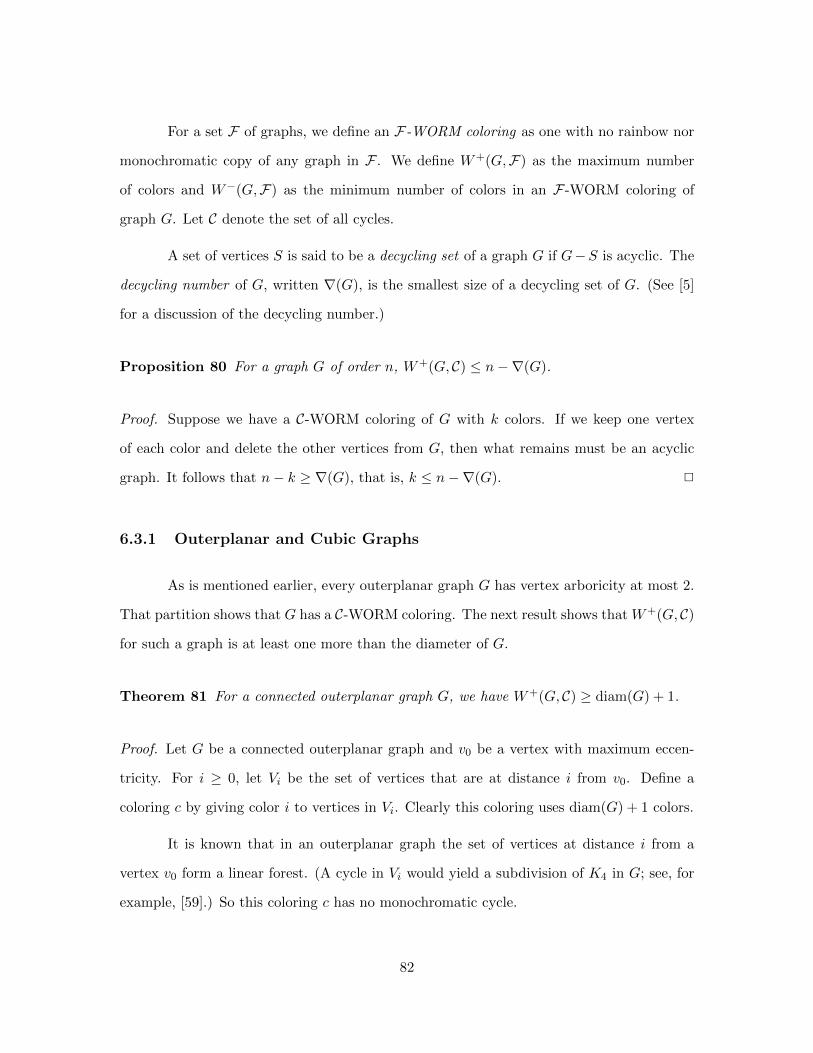
For a set F of graphs, we define an F-WORM coloring as one with no rainbow nor

monochromatic copy of any graph in F . We define W+(G,F) as the maximum number

of colors and W−(G,F) as the minimum number of colors in an F-WORM coloring of

graph G. Let C denote the set of all cycles.

A set of vertices S is said to be a decycling set of a graph G if G−S is acyclic. The

decycling number of G, written ∇(G), is the smallest size of a decycling set of G. (See [5]

for a discussion of the decycling number.)

Proposition 80 For a graph G of order n, W+(G, C) ≤ n−∇(G).

Proof. Suppose we have a C-WORM coloring of G with k colors. If we keep one vertex

of each color and delete the other vertices from G, then what remains must be an acyclic

graph. It follows that n− k ≥ ∇(G), that is, k ≤ n−∇(G). 2

6.3.1 Outerplanar and Cubic Graphs

As is mentioned earlier, every outerplanar graph G has vertex arboricity at most 2.

That partition shows that G has a C-WORM coloring. The next result shows that W+(G, C)

for such a graph is at least one more than the diameter of G.

Theorem 81 For a connected outerplanar graph G, we have W+(G, C) ≥ diam(G) + 1.

Proof. Let G be a connected outerplanar graph and v0 be a vertex with maximum eccen-

tricity. For i ≥ 0, let Vi be the set of vertices that are at distance i from v0. Define a

coloring c by giving color i to vertices in Vi. Clearly this coloring uses diam(G) + 1 colors.

It is known that in an outerplanar graph the set of vertices at distance i from a

vertex v0 form a linear forest. (A cycle in Vi would yield a subdivision of K4 in G; see, for

example, [59].) So this coloring c has no monochromatic cycle.

82

Further, a rainbow subgraph has at most one vertex from each Vi. Since there is no

edge between Vi and Vj for |i− j| ≥ 2, it follows that all rainbow subgraphs are paths. In

particular there is no rainbow cycle. 2

By Theorem 73, we have equality in the above theorem for MOPs of maximum

diameter (that is, MOPs of diameter bn/2c). However, the bound does not appear sharp

if one forbids only a specific cycle, such as C4. For example, computer search shows that

W+(G,C4) = 7 for every MOP G of order 9.

Similarly, since cubic graphs have vertex arboricity 2 (or by Lovasz’ result [58]), it

follows that W−(G, C) ≤ 2 for a cubic graph G. Here is one calculation for W+(G, C):

Observation 82 If G is the Petersen graph, then W+(G, C) = 7.

Proof. Since the order of the Petersen graph is 10, and the decycling number of the Petersen

graph is 3 (see, for example, [4]), it follows from Proposition 80 that W+(G, C) ≤ 7.

For the lower bound, take a maximum independent set I (which has size 4) and color

all of its vertices red while giving all other vertices distinct colors. Since this is a proper

coloring, there is no monochromatic cycle. Also there is no rainbow cycle, since every cycle

in G intersects I in at least two vertices. 2

We consider next the question for cubic graphs forbidding only the 4-cycle. The

maximum value of W+(G,C4) for cubic graphs G on n vertices is n. This value is achieved

by C4-free cubic graphs. For the minimum value of W+(G,C4) for cubic graphs G of order n,

we have the following conjecture:

Conjecture 8 For every cubic graph G of order n, W+(G,C4) ≥ 2n/3.

This value is achieved by the following graph: take r disjoint copies of K3,3− e and

add edges so that the resultant graph Br is cubic and connected. For example, B2 is drawn

in Figure 6.2. The graph Br has 6r vertices and one can calculate that W+(Br, C4) = 4r. A

83

computer search shows that B2 is indeed the unique (connected) cubic graph G of order 12

with minimum W+(G,C4).

Figure 6.2: The graph having minimum W+(G,C4) over cubic graphs of order 12

6.3.2 Cartesian Products

For the Cartesian product G2H to have a C4-WORM coloring, it is of course

necessary that both G and H have a C4-WORM coloring. However, we have not been able

to show that this condition is sufficient, nor could we find an example to the contrary.

We first consider grids. Let Gm,n denote the grid formed by the cartesian product

of Pm and Pn. We need the observation below. Recall that a set S bi-covers a subgraph H

if at least two vertices of H are in S. For positive integer s, bF (s) is the maximum number

of copies of F that can be bi-covered by using a set of size s.

Observation 83 For any grid and s > 0, bC4(s) ≤ 2(s− 1).

Proof. We prove this bound by induction. Let S be a set of s vertices. The bound is

immediate when S is contained in only one row. Now suppose S intersects at least two

rows. Let S1 be a maximal set of consecutive vertices of S in the topmost row of S. By the

induction hypothesis, the number of C4’s that contain at least two vertices in S \ S1 is at

most 2(|S| − |S1|) − 2. Further, the number of C4’s that contain at least one vertex in S1

and at least two vertices in S is at most 2|S1|: there are |S1| − 1 possible copies above S1

and at most |S1| + 1 copies below. Hence, the number of C4’s that S bi-covers is at most

2(|S| − |S1|)− 2 + 2|S1| = 2|S| − 2. 2

For grid graphs we have the following theorem. It was stated as a conjecture in [37],

and the lower bound was also proved there. The upper bound was proved in [40].

84

Theorem 84 (see [37, 40]) For G the m× n grid,

W+(G,C4) =

⌊(m+ 1)(n+ 1)

2

⌋− 1.

Proof. We first prove the lower bound by constructing a suitable coloring. Think of the

grid as having m rows numbered 1 up to m, and n columns numbered 1 up to n. There are

two cases.

Consider first the case that at least one of m or n is odd, say m. Then in each

odd-numbered row, give every vertex a unique color. For even-numbered rows, give every

vertex the same color. This coloring has no monochromatic cycle, no rainbow cycle, and

uses n(m+ 1)/2 + (m− 1)/2 = (m+ 1)(n+ 1)/2− 1 colors.

Consider second the case that both m and n are even. Then color all but the last

two rows as before: in each odd-numbered row give every vertex a unique color, and in

even-numbered rows give every vertex the same color. For the last two rows, do the same

coloring but based on columns: that is, in each odd-numbered column give both vertices a

unique color, and in even-numbered columns give both vertices the same color. The coloring

for m = n = 6 with 23 colors is illustrated in Figure 6.3, where • means that the vertex

receives a distinct color.

Figure 6.3: An optimal C4-WORM coloring of the 6× 6 grid

This coloring has no monochromatic cycle, no rainbow cycle, and uses n(m−2)/2+

85

(m− 2)/2 + 3(n/2) = (m+ 1)(n+ 1)/2− 3/2 colors.

The upper bound follows from Proposition 34 and Observation 83: in the m × n

grid, there are (m− 1)(n− 1) copies of C4, and so W+(G;C4) ≤ mn− (m− 1)(n− 1)/2 =

(m+ 1)(n+ 1)/2− 1. 2

We next consider rooks graphs.

Observation 85 The largest rooks graph that has a WORM C4-coloring is K92K9.

Proof. Note that any coloring of K10 must contain either a monochromatic C4 or a rain-

bow C4. On the other hand, a C4-WORM coloring of K92K9 is shown in the matrix

below.

1 1 1 2 2 2 3 3 3

3 3 3 1 1 1 2 2 2

2 2 2 3 3 3 1 1 1

1 2 3 1 2 3 1 2 3

3 1 2 3 1 2 3 1 2

2 3 1 2 3 1 2 3 1

1 2 3 2 3 1 3 1 2

3 1 2 1 2 3 2 3 1

2 3 1 3 1 2 1 2 3

(Note that the above is equivalent to a partition of the edge-set of K9,9 into three

C4-free cubic graphs. As such it was inspired by the construction used to prove the bipartite

Ramsey number b(2, 2, 2) ≥ 11; see [28, 36].) 2

6.4 Forbidding a Clique or Biclique

We consider first the case that the forbidden subgraph is a complete graph. It is

essentially a special case of the result on complete (l,m)-uniform mixed hypergraphs proved

by Tuza and Voloshin in [70]:

86

Theorem 86 (a) Kn has a Km-WORM coloring if and only if n ≤ (m− 1)2.

(b) In this range, W+(Kn,Km) = m− 1 and W−(Kn,Km) = dn/(m− 1)e.

Proof. (a) Assume Kn has a Km-WORM coloring. Let r be the number of colors; since

there is no rainbow Km, r ≤ m− 1. Since there is no monochromatic Km, each color class

contains at most m− 1 vertices. Hence n ≤ (m− 1)2. On the other hand, if n ≤ (m− 1)2,

then we use m− 1 colors as equitably as possible. This coloring has no monochromatic or

rainbow Km.

(b) Let r be the number of colors in a Km-WORM coloring of Kn. If r ≥ m, then

there is a rainbow Km. So W+ ≤ m− 1. Further, each color is used at most m− 1 times.

Therefore, r ≥ n/(m− 1).

(We note that we can have r as any value between dn/(m− 1)e and m− 1: just use

each of the r colors as equitably as possible.) 2

Part (a) of the above theorem can be extended to say that: if graph G has chromatic

number at most (m − 1)2, then it has a Km-WORM coloring. One just needs to color G

with m− 1 colors, giving all the vertices in m− 1 color classes the same color.

From this one can determine the maximum number of edges wex (n,Km) in a graph

of n vertices that has a Km-WORM coloring.

Theorem 87 The value wex (n,Km) equals the maximum number of edges in a K(m−1)2+1-

free graph.

Proof. Let G be a graph on n vertices with a Km-WORM coloring. By Theorem 86, G

does not contain K(m−1)2+1 as a subgraph. Thus wex (n,Km) is at most the Turan number

ex(n,K(m−1)2+1). Further, the Turan graphs are complete (m−1)2-partite graphs and thus,

by the above discussion, have a Km-WORM coloring. 2

We consider next the case that the forbidden subgraph is a complete bipartite graph.

Trivially, the bipartite coloring of a bipartite graph is automatically an F -WORM col-

87

oring. So we focus on the maximum number of colors. In Chapter 5 we proved that

W+(Kn,n,K1,m) = 2m− 2 for n ≥ m ≥ 2. One can extend that as follows:

Theorem 88 For n ≥ m ≥ 2, W+(Kn,n,Km,m) = n+m− 1.

Proof. For the lower bound, color red n−m+ 2 vertices in one of the partite set, and give

every other vertex a distinct color. This uses 2n+ 1− (n−m+ 2) = n+m− 1 colors, and

is a Km,m-WORM coloring (since one partite set contains only m− 1 colors).

On the other hand, consider a Km,m-WORM coloring of Kn,n that uses at least

m + n colors. Then each partite set has at least m colors that do not appear in the other

partite set. This immediately gives a rainbow Km,m. That is, W+(Kn,n,Km,m) ≤ n+m−1.

2

6.5 Minimal Colorings

For graphs that do not have WORM colorings, one can ask how close to WORM

can one get. We call a subgraph bad if it is rainbow or monochromatic, and define B(G,F )

as the minimum number of bad subgraphs isomorphic to F in a coloring of G. In particular,

B(G,F ) = 0 means there is an F -WORM coloring of G.

Theorem 86 says that B(Kn,Km) ≥ 1 if n ≥ (m− 1)2 + 1. One can ask what is the

exact value of B(Kn,Km) in this case. We show that an optimal coloring uses m− 1 colors

as equitably as possible.

Theorem 89 Let n = (m − 1)k + j with 0 ≤ j ≤ m − 2. Then B(Kn,Km) = j(k+1m

)+

(m− 1− j)(km

).

Proof. Let an optimal coloring of Kn be given. Assume that color i is used ai times with

a1 ≤ a2 ≤ . . . ≤ ar.

88

Suppose that r ≥ m. Assume we recolor one vertex that has color 1 with color 2;

let M denote the increase in the the number of monochromatic Km’s and R the decrease

in the number of rainbow Km’s. Then

M =

(a1 − 1

m

)−(a1m

)+

(a2 + 1

m

)−(a2m

)≤(a2 + 1

m

)−(a2m

)=

(a2

m− 1

)≤ a2m−1,

and

R = a2∑

3≤i1≤...≤im−2≤rai1 . . . aim−2 ≥ a2a3 . . . am ≥ a2m−1.

That is, M ≤ R. Hence the total number of bad Km’s will not increase.

By repeating the argument, it follows that we may recolor all the vertices with color 1

and so reduce the total number of colors used. That is, we may assume that r ≤ m − 1.

In this case, rainbow Km’s are impossible and thus we have only to minimize the number

of monochromatic Km’s. By convexity of the function f(x) =(xm

), optimality is achieved

when m− 1 colors are used as equitably as possible. 2

89

Chapter 7

Vertex Colorings without Rainbow

or Monochromatic Subgraphs

7.1 Introduction

This chapter is based on joint work with Wayne Goddard [40]. As all proofs in the

original paper are provided, we do not give specific references to that paper.

In Chapter 5 and Chapter 6, we considered WORM colorings: these forbid both a

rainbow and a monochromatic copy of a specific subgraph. But it is more flexible to allow

different restrictions. For graphs M and R, we define an (M,R)-WORM coloring of G to be

a coloring of the vertices of G with neither a monochromatic subgraph isomorphic to M nor

a rainbow subgraph isomorphic to R. As is mentioned in Chapter 4, this coloring is a special

case of colorings of mixed hypergraphs introduced by Voloshin; see for example [74, 75, 71].

Note that when M = R, this is just the WORM colorings we studied in Chapter 5 and

Chapter 6.

One special case of such colorings has a distinguished history. Erdos et al. [26]

defined the local chromatic number of a graph as the maximum order of a rainbow star that

must appear in all proper colorings. In our notation, this is the minimum r such that the

90

graph has an (K2,K1,r+1)-WORM coloring. For a survey on this parameter, see [61].

A related question studied in the edge case is the rainbow Ramsey number (or

constrained Ramsey number); this is defined as the minimum N such that any coloring of

the edges of KN produces either a monochromatic M or a rainbow R. See [27].

One case of (M,R)-WORM colorings is trivial: if we forbid a rainbow K2, then every

component of the graph must be monochromatic. Similarly, if we forbid a rainbow kK1,

then this is equivalent to using less than k colors. So we will assume that the subgraph R

has at least three vertices and at least one edge. On the other hand, taking M = K2 is

equivalent to insisting that the coloring is proper. Also, taking M = kK1 is equivalent to

using each color less than k times.

Having two competing restrictions leads naturally to considering both the minimum

and maximum number of colors in such a coloring. So we define the upper chromatic

number W+(G;M,R) as the maximum number of colors, and the lower chromatic number

W−(G;M,R) as the minimum number of colors, in an (M,R)-WORM coloring of G (if

the graph has such a coloring). For bounds, it will be useful to also let m−(G;M) be the

minimum number of colors without a monochromatic M , and r+(G;R) be the maximum

number of colors without a rainbow R. Note that

m−(G;M) ≤W−(G;M,R) ≤W+(G;M,R) ≤ r+(G;R),

provided G has an (M,R)-WORM coloring.

We proceed as follows: in Section 7.2 we give basic observations. In Section 7.3

we provide one general upper bound when R is a path. In Section 7.4 we consider proper

colorings without rainbow P3, P4, or C4. Finally, in Section 7.5 we provide a few results for

other cases.

91

7.2 Preliminaries

We start with some simple observations. If G is bipartite then the bipartition is

immediately an (M,R)-WORM coloring. Indeed, if G is k-colorable with k < |R| , then a

proper k-coloring of G is an (M,R)-WORM coloring. Also:

Observation 90 Fix graphs M and R and let G be a graph.

(a) If G has an (M,R)-WORM coloring, then so does G − e where e is any edge

and G− v where v is any vertex. Further, W+(G− e;M,R) ≥W+(G;M,R) and W+(G−

v;M,R) ≥W+(G;M,R)− 1, with similar results for the lower chromatic number.

(b) If M and R are connected but G is disconnected, then W+(G;M,R) is the sum

of the parameter for the components, and W−(G;M,R) is the maximum of the parameter

for the components.

(c) It holds that W+(G;M,R) = |V (G)| if and only if G is R-free.

(d) It holds that W+(G;M,R) ≥ |R| − 1 if G is |R| − 1 colorable (and has at least

that many vertices).

7.2.1 General M

It should be noted that maximizing the number of colors while avoiding a rainbow

subgraph can produce a large monochromatic subgraph. For example:

Observation 91 For all connected graphs M , there exists a graph G such that

W+(G;M,P3) < r+(G;P3).

Proof. In Chapter 4 we considered the corona cor(G) of a graph G; this is the graph

obtained from G by adding, for each vertex v in G, a new vertex v′ and the edge vv′. It was

shown that r+(G;P3) = |G|+ 1. In fact, we note here that if G is connected, then one can

92

readily show by induction that the optimal coloring is unique and gives every vertex of G

the same color. In particular, it follows that the no-rainbow-P3 coloring of cor(M) with the

maximum number of colors contains a monochromatic copy of M . 2

7.3 A Result on Rainbow Paths

We showed in Chapter 5 that a nontrivial graph G has a (P3, P3)-WORM coloring

if and only if it has one using at most two colors. We prove an analogue for general paths.

This result is a slight generalization of Theorem 10 in [70].

Theorem 92 Fix some graph M ; if graph G has an (M,Pr)-WORM coloring, then G has

one using at most r − 1 colors.

Proof. Consider an (M,Pr)-WORM coloring f of G. Let GM be the spanning subgraph of G

whose edges are monochromatic and GR the spanning subgraph whose edges are rainbow.

It follows that GM that does not contain M , and that GR does not contain Pr. By the

Gallai-Hasse-Roy-Vitaver theorem [34, 45, 66, 73], since GR does not contain Pr, it has

chromatic number at most r − 1.

Now, let g be a proper coloring of GR using at most r − 1 colors and consider g as

a coloring of G. Note that the monochromatic edges under g are a subset of the monochro-

matic edges under f . Therefore, g is a (M,Pr)-WORM coloring of G using at most r − 1

colors. 2

It follows that:

Corollary 93 For any graph M and r > 0, graph G has an (M,Pr)-WORM coloring if

and only if m−(G,M) ≤ r − 1. If so, W−(G;M,Pr) = m−(G,M).

On the other hand, Theorem 92 does not extend to stars. For example, Erdos et

al. [26] constructed a shift graph that has arbitrarily large chromatic number but can be

properly colored without a rainbow K1,3. That is:

93

Theorem 94 For r ≥ 3 and k ≥ 1, there is a graph G with W−(G;K2,K1,r) ≥ k.

Nor does Theorem 92 generalize to K3; see [11].

7.4 Proper Colorings

Recall that W+(G;K2, R) is the maximum number and W−(G;K2, R) is the mini-

mum number of colors in a proper coloring without a rainbow R.

7.4.1 Two simple cases

Two cases for M = K2 are immediate:

Observation 95 A graph G has a (K2, P3)-WORM coloring if and only if it is bipartite.

If so, W+(G;K2, P3) = W−(G;K2, P3) = 2, provided G is connected and nonempty.

Proof. If we have a (K2, P3)-WORM coloring, then for each vertex v all its neighbors must

have the same color, which is different to v’s color. It follows that every path must alternate

colors. 2

In a proper coloring of a graph, all cliques are rainbow. Thus it follows:

Observation 96 A graph G has a (K2,Km)-WORM coloring if and only if it is Km-free.

If so, W+(G;K2,Km) = |G| while W−(G;K2,Km) = χ(G).

7.4.2 No rainbow K1,3

Consider first that G is bipartite. Then in maximizing the colors, it is easy to see

that one may assume the colors in the partite sets are disjoint. (If red is used in both partite

sets, then change it to pink in one of the sets.) In particular, unless G is a star, one can use

94

at least two colors in each partite set. (This result generalizes to R any star.) For example,

it follows that W+(Km,m;K2,K1,3) = 4 for m ≥ 2.

Indeed, it is natural to consider the open neighborhood hypergraph ON(G) of the

graph G. This is the multihypergraph with vertex set V (G) and a hyperedge for every

open neighborhood in G. In general, since we have a proper coloring, the requirement of

no rainbow K1,r is equivalent to every hyperedge in ON(G) receiving at most r − 1 colors.

In the case that G is bipartite, the two problems are equivalent:

Observation 97 For any graph G, the parameter W+(G;K2,K1,r) is at most the maxi-

mum number of colors in a coloring of ON(G) with every hyperedge receiving at most r− 1

colors. Furthermore, there is equality if G is bipartite.

Proof. When G is bipartite, the ON(G) can be partitioned into two disjoint multihyper-

graphs and so will have disjoint colors in the multihypergraphs. It follows that the coloring

back in G will be proper. 2

Observation 98 If G is a 2-tree of order at least 3, then W+(G;K2,K1,3) = 3.

Proof. It is well known that any 2-tree is 3-colorable. Furthermore, it follows readily by

induction that a (K2,K1,3)-WORM coloring can use only three colors: when we add a

vertex v and join it to adjacent vertices x and y, they already have a common neighbor z,

and so v must get the same color as z. 2

Osang showed that determining whether a graph has a (K2,K1,3)-WORM coloring

is hard:

Theorem 99 [61] Determining whether a graph has a (K2,K1,3)-WORM coloring is NP-

complete.

95

7.4.2.1 Cubic graphs

We next consider cubic graphs. It is easy to see that K4 does have a (K2,K1,3)-

WORM coloring. On the other hand, by Brooks’ Theorem [8], every cubic graph other

than K4 has a proper coloring using at most 3 colors. Note that such a proper coloring is

also a (K2,K1,3)-WORM coloring. Further, they have a coloring using two colors if and only

if they are bipartite. So the only interesting question is the behavior of W+(G;K2,K1,3).

Observation 100 If G is cubic of order n, then W+(G;K2,K1,3) ≤ 2n/3.

Proof. Since G is cubic, the open neighborhood hypergraph ON(G) is 3-regular and 3-

uniform. Further we need a coloring of ON(G) where every hyperedge has at least one pair

of vertices the same color. Consider some color used more than once, say red. If there are r

red vertices, then at most 3r/2 hyperedges can have at least two red vertices. (Each vertex

is contained in at most three hyperedges.)

It follows that if the ith non-unique color is used ri times, then we need∑

i ri ≥ 2n/3.

Let B be the number of vertices that can be discarded and still have one vertex of each

color. Then B =∑

i(ri − 1) and by above B ≥ n/3. It follows that the total number of

colors is at most 2n/3. 2

Equality in Observation 100 is obtained by taking disjoint copies of K3,3 − e and

adding edges to make the graph connected. See Figure 7.1.

Consider next the minimum value of W+(G;K2,K1,3) for cubic graphs of order n.

We noted above that bipartite graphs in general have a value of at least 4. Computer search

shows that this parameter is at least 3 for n ≤ 18. Indeed, it finds only three graphs where

the parameter is 3: one of order 6 (the prism), one of order 10, and one of order 14 (the

generalized Petersen graph). These three graphs are shown in Figure 7.2.

The general case remains open.

96

Figure 7.1: A cubic graph G with W+(G;K2,K1,3) two-thirds its order

Figure 7.2: The known cubic graphs with W+(G;K2,K1,3) = 3

7.4.3 Forbidding rainbow P4

We consider proper colorings without rainbow P4’s, then Theorem 92 applies. That

is, a graph G has a (K2, P4)-WORM coloring if and only if G has chromatic number at

most 3. Since it is NP-complete to determine if a graph has a proper 3-coloring [35], it

follows that it is also NP-complete to determine if a graph has a (K2, P4)-WORM coloring.

Further, if such a coloring exists, then W−(G;K2, P4) is just the chromatic number of G.

So we consider only the upper chromatic number here.

Observation 101 If graph G is bipartite of order n, then W+(G;K2, P4) ≥ n/2 + 1.

Proof. In the smaller partite set, give all vertices the same color, and in the other partite

set, give all vertices unique colors. Note that every copy of P4 contains two vertices from

both partite sets. 2

97

Observation 102 If connected graph G of order n has a perfect matching, then it holds

that W+(G;K2, P4) ≤ n/2 + 1.

Proof. Number the edges of the perfect matching e1, . . . , en/2 such that for all i > 1, at

least one endpoint of ei is connected to some ej for j < i through another edge. Then ei,

ej , and the connecting edge form a P4. It follows that ej and ei share a color. Thus the

total number of colors used is at most 2 + (n/2− 1) = n/2 + 1. 2

For example, equality is obtained in both observations for any connected bipar-

tite graph with a perfect matching, such as the balanced complete bipartite graph or the

path/cycle of even order. Equality is also obtained in Observation 101 for the tree of diam-

eter three where the two central vertices have the same degree. Also, there are nonbipartite

graphs that achieve equality in Observation 102; for example, the graph shown in Figure 7.3.

Figure 7.3: A nonbipartite graph G with a perfect matching and maximum W+(G;K2, P4)

We determine next the parameter for the odd cycle:

Observation 103 If n is odd, then W+(Cn;K2, P4) is 3 for n ≤ 5, and (n−1)/2 for n ≥ 7.

Proof. The result for n = 3 is trivial and for n = 5 is easily checked. So assume n ≥ 7. For

the lower bound, color a maximum independent set red, give a new color to every vertex

with two red neighbors, and color each vertex with one red neighbor the same color as on

the other side of its red neighbor. For example, the coloring for C13 is shown in Figure 7.4

(where the red vertices are shaded).

We now prove the upper bound. Two same-colored vertices distance 2 apart bi-cover

two copies of P4, while two same-covered vertices distance 3 apart bi-cover one copy. It

follows that if a color is used k times, it can bi-cover at most 2(k− 1) copies of P4, except if

98

15

1

2

3

4

5

Figure 7.4: Coloring showing W+(C13;K2, P4)

the vertices of that color form a maximum independent set, when it bi-covers 2k− 1 copies.

Since there are n copies of P4 in total, by Proposition 34 it follows that the total number

of colors is at most n/2, unless some color is a maximum independent set. So say red is

a maximum independent set. Let b and e be the two red vertices at distance 3; say the

portion of the cycle containing them is abcdef . By considering the a–d copy of P4, it follows

that a must have the same color as c or d. Similarly, f must have the same color as c or d.

Thus the total number of colors is at most 1 + (n− (n− 1)/2)− 2 = (n− 1)/2. 2

In contrast to Observation 101, we get the following:

Theorem 104 If connected graph G has every vertex in a triangle, then W+(G;K2, P4) = 3

if such a coloring exists.

Proof. Note that every triangle is properly colored. We show that every triangle receives

the same three colors. Consider two triangles T1 and T2. If T1 and T2 share two vertices,

then the third vertex in each share a color. Consider the case that T1 and T2 share one

vertex. Then by considering the four P4’s using all vertices but one, it readily follows that

the triangles must have the same colors.

Now, assume that T1 and T2 are disjoint but joined by an edge e. Suppose they do

not have the same three colors. Then there is vertex u1 in T1 and u2 in T2 that do not share

a color with the other triangle. If u1 and u2 are the ends of e, then any P4 starting with e

is rainbow. If u1 and u2 are not the ends of e, then there is a P4 whose ends are u1 and u2

99

and that P4 must be rainbow. Either way, we obtain a contradiction.

Since the graph is connected, it follows that every triangle is colored with the same

three colors. Since this includes all the vertices, the result follows. 2

From the above theorem, it follows that W+(G;K2, P4) = 3 for every maximal

outerplanar graph G.

7.4.3.1 Cubic Graphs

There are many cubic graphs with W+(G;K2, P4) = 3. These include, for example,

the cubic graphs that do not contain K1,3 as an induced subgraph (equivalently the ones

where every vertex is in a triangle). See Theorem 104.

For the largest value of the parameter, computer evidence suggests:

Conjecture 9 If G is a connected cubic graph of order n, then W+(G;K2, P4) ≤ n/2 + 1,

with equality exactly when G is bipartite.

Certainly, by Observations 101 and 102 (and the fact that regular bipartite graphs

have perfect matchings), that value is achieved by all bipartite cubic graphs.

7.4.4 Forbidding rainbow C4

We conclude this section by considering proper colorings without rainbow 4-cycles.

Observation 105 For every maximal outerplanar graph G, it holds that

W−(G;K2, C4) = W+(G;K2, C4) = 3.

Proof. Consider two triangles sharing an edge. Then, to avoid a rainbow C4, the two

vertices not on the edge must have the same color. It follows that all triangles have the

same three colors. 2

100

We next consider cubic graphs. It is easy to see that K4 does have a (K2, C4)-

WORM coloring. On the other hand, by Brooks’ Theorem [8], every cubic graph other

than K4 has a proper coloring using at most 3 colors. Note that such a proper coloring is

also a (K2, C4)-WORM coloring. Thus, W−(G;K2, C4) = 2 if G is a bipartite cubic graph,

and W−(G;K2, C4) = 3 if G is a nonbipartite cubic graph other than K4. Further, the

upper bound for W+(G;K2, C4) is trivial: one can have a cubic graph without a 4-cycle.

Computer evidence suggests that:

Conjecture 10 If G is a connected cubic graph of order n ≥ 6, then W+(G;K2, C4) ≥ n/2.

This lower bound is achievable. For n even, a Mobius ladder is defined by taking the

cycle on n vertices and joining every pair of opposite vertices. Note that a Mobius ladder

is bipartite when its order is not a multiple of 4; while a prism is bipartite when its order

is a multiple of 4.

Observation 106 If G is a nonbipartite Mobius ladder or nonbipartite prism of order n,

then it holds that W+(G;K2, C4) = n/2.

Proof. We first exhibit the coloring. Let m = n/2. Say the vertices of the prism are

u1, . . . , um and v1, . . . , vm, where ui has neighbors ui−1, ui+1, and vi (arithmetic modulo m)

and similarly for vi. Then for 1 ≤ i ≤ m, give vertices ui and vi+1 color i.

Say the vertices of the Mobius ladder are w1, . . . , wn where wi has neighbors wi−1,

wi+1, and wi+m (arithmetic modulo n). Then for 2 ≤ i ≤ m, give vertices wi and wi+m−1

color i, give vertex w1 color 1 and give vertex wn color 2. For example, the coloring for the

case n = 12 is shown in Figure 7.5.

Now, for the upper bound, consider a color that is used r times. A color bi-covers

a copy of C4 if it contains vertices from consecutive rungs (where a rung is an edge in

two C4’s). Since the graph is not bipartite, the color cannot be present in every rung. It

101

2

2

3

3

4

4

5

5

6

6

1

2

Figure 7.5: Coloring of Mobius ladder

follows that it can bi-cover at most r − 1 copies of C4. Now, there are m copies of C4

(note that the prism of C4 is bipartite so excluded). It follows from Proposition 34 that the

number of colors is at most n− n/2 = n/2. 2

7.5 Other Results

7.5.1 Paths and paths

The natural strategy to color a long path without a rainbow Pr yields the following

result. It can also be obtained as a special case of the result on interval mixed hypergraphs

given in [13]:

Observation 107 For any m ≥ 3, it holds that W+(Pn;Pm, Pr) = r+(Pn;Pr) = b(r −

2)n/(r − 1)c+ 1.

Proof. Give the first r − 1 vertices different colors, then the next vertex the same color as

the previous vertex, then the next r − 2 vertices different colors, and so on. This coloring

has a monochromatic P2 but not a monochromatic P3, and is easily seen to be best possible

(as every copy of Pr must contain two vertices of the same color). 2

7.5.2 Bicliques and bicliques

Next we revisit the case that G, M , and R are bicliques. For n ≥ b it was proved

that W+(Kn,n;K1,b,K1,b) = 2b−2 in [38] and that W+(Kn,n;Kb,b,Kb,b) = n+ b−1 in [37].

The case for stars is special, but it is straight-forward to generalize the latter:

102

Theorem 108 Let m ≤ n and 2 ≤ a ≤ b with m ≥ a and n ≥ b. Then

r+(Km,n;Ka,b) = max(a+ n− 1, b− 1 + min(m, b− 1)).

Proof. Consider a coloring Km,n without a rainbow Ka,b and assume there are at least a+ b

colors. If we can choose a colors from one partite set and b colors from the other that are

disjoint, then we would obtain a rainbow Ka,b. So either there is a partite set that has at

most a−1 colors that do not appear in the other partite set, or each partite set has at most

b− 1 colors. In the first case, the maximum number of colors possible is a+ n− 1. In the

second case, the maximum number of colors possible is b− 1 + min(m, b− 1). The theorem

follows. 2

Note that in the above proof, the optimal number of colors can be achieved by

making the sets of colors in the two partite sets disjoint. Thus, one obtains a similar value

for W+(Km,n;M,Ka,b) where M is any nontrivial biclique.

7.6 Other Directions

We conclude with some thoughts on future directions. Apart from the specific open

problems raised here, a direction that looks interesting is the case where M and R are both

stars. Also of interest is the case that the host graph is a product graph.

103

Chapter 8

Conclusion and Future Directions

of Research

In this thesis, we studied several types of generalized vertex colorings of graphs.

We studied fractional and circular chromatic numbers and the defective version

of these parameters for series-parallel graphs. In particular, we showed that the fractional

chromatic number of any series-parallel graph of odd girth k is exactly 2k/(k−1), confirming

a conjecture by Wang and Yu. We also showed that for every d there is a series-parallel

graph whose d-defective fractional and circular chromatic numbers are both 3, answering

a question of Klostermeyer. Note that simple series-parallel graphs are also the partial

2-trees. So it is natural to consider partial k-trees in general. Chlebıkova [18] showed that

for k ≥ 3, every triangle-free partial k-tree has chromatic number at most k. It would be

interesting to investigate if this is best possible and what happens for fractional/circular

coloring and/or higher girth/odd girth.

We introduced the concept of fractional defect. We established some basic properties

of this concept, and investigated the minimum fractional defect over a few families of graphs,

giving exact values in some cases and bounds in others. The problem is NP-hard in general,

and it seems to be nontrivial even for some graphs that have simple structures. It is

104

quite possible that more advanced tools or techniques are required to make progress on

the conjectures and open problems that we proposed. One of the problems that seems

interesting to us is to determine the minimum fractional defect for the rooks graph Km2Kn

where one of m and n is odd.

We considered several types of vertex colorings of a graph forbidding rainbow or

monochromatic subgraphs. We presented some results especially with regards to the ex-

istence of colorings, complexity, and optimization within certain graph classes. Our focus

was on the case that the forbidden subgraph is a path, cycle, star, or clique. One possible

direction of future research would be to attack the specific conjectures and open problems

raised in Chapters 4, 5, 6, 7 of the thesis, for example, those conjectures that concern ex-

tremal values of number of colors in no-rainbow-colorings of cubic graphs of fixed order.

Another possible direction of future research would be to consider other types of forbidden

subgraphs. Finally, the gap of chromatic spectrum seems to be an interesting direction.

In particular, Bujtas and Tuza [11] proposed the following conjecture: for every integer

k ≥ 4, there exists a K3-WORM-colorable K4-free graph G such that W−(G,K3) = k.

This conjecture, if true, would extend Theorem 79.

105

Bibliography

[1] M. Axenovich and P. Iverson. Edge-colorings avoiding rainbow and monochromaticsubgraphs. Discrete Math., 308(20):4710–4723, 2008.

[2] M. Axenovich, T. Jiang, and P. Iverson. Bipartite anti-Ramsey numbers of cycles. J.Graph Theory, 47:9–28, 2004.

[3] M. Axenovich and R. Martin. Avoiding rainbow induced subgraphs in vertex-colorings.Electron. J. Combin., 15(1):Research Paper 12, 23, 2008.

[4] S. Bau and L. W. Beineke. The decycling number of graphs. Australas. J. Combin.,25:285–298, 2002.

[5] L.W. Beineke and R.C. Vandell. Decycling graphs. J. Graph Theory, 25(1):59–77,1997.

[6] O.V. Borodin, A.O. Ivanova, M. Montassier, P. Ochem, and A. Raspaud. Vertexdecompositions of sparse graphs into an edgeless subgraph and a subgraph of maximumdegree at most k. J. Graph Theory, 65:83–93, 2010.

[7] I. Broere and C.M. Mynhardt. Generalized colorings of outerplanar and planar graphs.In Graph theory with applications to algorithms and computer science (Kalamazoo,Mich., 1984), pages 151–161. Wiley, New York, 1985.

[8] R.L. Brooks. On colouring the nodes of a network. Proc. Cambridge Philos. Soc.,37:194–197, 1941.

[9] Cs. Bujtas, E. Sampathkumar, Zs. Tuza, C. Dominic, and L. Pushpalatha. Vertexcoloring without large polychromatic stars. Discrete Math., 312:2102–2108, 2012.

[10] Cs. Bujtas, E. Sampathkumar, Zs. Tuza, M.S. Subramanya, and C. Dominic. 3-consecutive C-colorings of graphs. Discuss. Math. Graph Theory, 30:393–405, 2010.

[11] Cs. Bujtas and Zs. Tuza. K3-WORM colorings of graphs: Lower chromatic numberand gaps in the chromatic spectrum. arXiv:1508.01759.

[12] Cs. Bujtas and Zs. Tuza. Maximum number of colors: C-coloring and related problems.J. Geom., 101(1-2):83–97, 2011.

106

[13] E. Bulgaru and V. Voloshin. Mixed interval hypergraphs. Discrete Appl. Math.,77(1):29–41, 1997.

[14] G.J. Chang and G.L. Nemhauser. The k-domination and k-stability problems on sun-free chordal graphs. SIAM J. Algebraic Discrete Methods, 5(3):332–345, 1984.

[15] G. Chartrand and F. Harary. Planar permutation graphs. Ann. Inst. H. Poincare Sect.B (N.S.), 3:433–438, 1967.

[16] G. Chartrand and H.V. Kronk. The point-arboricity of planar graphs. J. London Math.Soc., 44:612–616, 1969.

[17] G. Chartrand and P. Zhang. Chromatic graph theory. Discrete Mathematics and itsApplications (Boca Raton). CRC Press, Boca Raton, FL, 2009.

[18] J. Chlebıkova. Partial k-trees with maximum chromatic number. Discrete Math.,259:269–276, 2002.

[19] J. Cooper, F. Stephen, and S. Purewal. Monochromatic boxes in colored grids. SIAMJ. Discrete Math., 25(3):1054–1068, 2011.

[20] L.J. Cowen, R.H. Cowen, and D.R. Woodall. Defective colorings of graphs in surfaces:partitions into subgraphs of bounded valency. J. Graph Theory, 10:187–195, 1986.

[21] L.J. Cowen, W. Goddard, and C. E. Jesurum. Defective coloring revisited. J. GraphTheory, 24(3):205–219, 1997.

[22] R.H. Cowen. Some connections between set theory and computer science. In Compu-tational logic and proof theory (Brno, 1993), volume 713 of Lecture Notes in Comput.Sci., pages 14–22. Springer, Berlin, 1993.

[23] D.W. Cranston, J. Kim, and W.B. Kinnersley. New results in t-tone coloring of graphs.Electron. J. Combin., 20:Paper 17, 14, 2013.

[24] Z. Dvorak, D. Kral, and R. Skrekovski. Non-rainbow colorings of 3-, 4- and 5-connectedplane graphs. J. Graph Theory, 63:129–145, 2010.

[25] Z. Dvorak, D. Kral, and J. Teska. Toughness threshold for the existence of 2-walks inK4-minor-free graphs. Discrete Math., 310(3):642–651, 2010.

[26] P. Erdos, Z. Furedi, A. Hajnal, P. Komjath, V. Rodl, and A. Seress. Coloring graphswith locally few colors. Discrete Math., 59:21–34, 1986.

[27] L. Eroh. Constrained Ramsey numbers of matchings. J. Combin. Math. Combin.Comput., 51:175–190, 2004.

[28] G. Exoo. A bipartite Ramsey number. Graphs Combin., 7(4):395–396, 1991.

[29] Z. Farkasova and R. Sotak. Fractional and circular 1-defective colorings of outerplanargraphs. Australas. J. Combin., 63:1–11, 2015.

107

[30] O. Favaron. Signed domination in regular graphs. Discrete Math., 158:287–293, 1996.

[31] T. Feder and C. Subi. Bipartite subgraphs of large odd girth series-parallel graphs.preprint.

[32] G. Fertin, E. Godard, and A. Raspaud. Acyclic and k-distance coloring of the grid.Inform. Process. Lett., 87(1):51–58, 2003.

[33] S. Fujita, C. Magnant, and K. Ozeki. Rainbow generalizations of Ramsey theory: asurvey. Graphs Combin., 26:1–30, 2010.

[34] T. Gallai. On directed paths and circuits. Theory of graphs, pages 115–118, 1968.

[35] M.R. Garey and D.S. Johnson. Computers and intractability. W. H. Freeman and Co.,San Francisco, Calif., 1979. A guide to the theory of NP-completeness, A Series ofBooks in the Mathematical Sciences.

[36] W. Goddard, M.A. Henning, and O.R. Oellermann. Bipartite Ramsey numbers andZarankiewicz numbers. Discrete Math., 219(1):85–95, 2000.

[37] W. Goddard, K. Wash, and H. Xu. WORM colorings forbidding cycles or cliques.Congr. Numer., 219:161–173, 2014.

[38] W. Goddard, K. Wash, and H. Xu. WORM colorings. Discuss. Math. Graph Theory,35:571–584, 2015.

[39] W. Goddard and H. Xu. Colorings with fractional defect. Submitted.

[40] W. Goddard and H. Xu. Vertex colorings without rainbow or monochromatic sub-graphs. To appear in J. Combin. Math. Combin. Comput.

[41] W. Goddard and H. Xu. Vertex colorings without rainbow subgraphs. To appear inDiscuss. Math. Graph Theory.

[42] W. Goddard and H. Xu. Fractional, circular, and defective coloring of series-parallelgraphs. J. Graph Theory, 81(2):146–153, 2016.

[43] A. Gyarfas, G. N. Sarkozy, A. Sebo, and S. Selkow. Ramsey-type results for Gallaicolorings. J. Graph Theory, 64:233–243, 2010.

[44] A. Gyarfas and G. Simony. Edge colorings of complete graphs without tricoloredtriangles. J. Graph Theory, 46:211–216, 2004.

[45] M. Hasse. Zur algebraischen begrundung der graphentheorie. I. MathematischeNachrichten, 28(5-6):275–290, 1965.

[46] S.M. Hedetniemi, A. Proskurowski, and M.M. Sys lo. Interior graphs of maximal out-erplane graphs. J. Combin. Theory Ser. B, 38(2):156–167, 1985.

[47] P. Hell and X. Zhu. The circular chromatic number of series-parallel graphs. J. GraphTheory, 33:14–24, 2000.

108

[48] R.E. Jamison and G.L. Matthews. Distance k colorings of Hamming graphs. In Proceed-ings of the Thirty-Seventh Southeastern International Conference on Combinatorics,Graph Theory and Computing, volume 183, pages 193–202, 2006.

[49] T.R. Jensen and B. Toft. Graph coloring problems. Wiley-Interscience Series in DiscreteMathematics and Optimization. John Wiley & Sons, Inc., New York, 1995. A Wiley-Interscience Publication.

[50] M. Juvan, B. Mohar, and R. Thomas. List edge-colorings of series-parallel graphs.Electron. J. Combin., 6:Research Paper 42, 6 pp. (electronic), 1999.

[51] A. Kemnitz and P. Wellmann. Circular chromatic numbers of certain planar graphs.Congr. Numer., 169:199–209, 2004.

[52] A. Kisielewicz and M. Szyku la. Rainbow induced subgraphs in proper vertex colorings.Fund. Inform., 111:437–451, 2011.

[53] W. Klostermeyer. Defective circular coloring. Australas. J. Combin., 26:21–32, 2002.

[54] W. Klostermeyer and C.Q. Zhang. (2+ε)-coloring of planar graphs with large odd-girth.J. Graph Theory, 33:109–119, 2000.

[55] F. Kramer and H. Kramer. A survey on the distance-colouring of graphs. DiscreteMath., 308(2-3):422–426, 2008.

[56] K.W. Lih, C.Y. Lin, and L.D. Tong. On an interpolation property of outerplanargraphs. Discrete Applied Math., 154(1):166–172, 2006.

[57] D.D. Liu and X. Zhu. Fractional chromatic number and circular chromatic number fordistance graphs with large clique size. J. Graph Theory, 47:129–146, 2004.

[58] L. Lovasz. On decomposition of graphs. Studia Sci. Math. Hungar., 1:237–238, 1966.

[59] P. Mihok. On vertex partition numbers of graphs. In Graphs and other combinatorialtopics (Prague, 1982), pages 183–188. Teubner, Leipzig, 1983.

[60] P. Mihok, J. Oravcova, and R. Sotak. Generalized circular colouring of graphs. Discuss.Math. Graph Theory, 31:345–356, 2011.

[61] G. Osang. The local chromatic number. Master’s thesis, University of Waterloo, 2013.

[62] Z. Pan and X. Zhu. The circular chromatic number of series-parallel graphs of largeodd girth. Discrete Math., 245:235–246, 2002.

[63] Z. Pan and X. Zhu. Tight relation between the circular chromatic number and thegirth of series-parallel graphs. Discrete Math., 254:393–404, 2002.

[64] A. Pirnazar and D.H. Ullman. Girth and fractional chromatic number of planar graphs.J. Graph Theory, 39:201–217, 2002.

[65] R. Ramamurthi and D.B. West. Maximum face-constrained coloring of plane graphs.Discrete Math., 274:233–240, 2004.

109

[66] B. Roy. Nombre chromatique et plus longs chemins d’un graphe. ESAIM: MathematicalModelling and Numerical Analysis-Modelisation Mathematique et Analyse Numerique,1(5):129–132, 1967.

[67] E.R. Scheinerman and D.H. Ullman. Fractional graph theory: A rational approach tothe theory of graphs. Courier Dover Publications, 2011.

[68] J.A. Telle and A. Proskurowski. Algorithms for vertex partitioning problems on partialk-trees. SIAM J. Discrete Math., 10(4):529–550, 1997.

[69] Zs. Tuza. Graph colorings with local constraints—a survey. Discuss. Math. GraphTheory, 17(2):161–228, 1997.

[70] Zs. Tuza and V. Voloshin. Uncolorable mixed hypergraphs. In Proceedings of the5th Twente Workshop on Graphs and Combinatorial Optimization (Enschede, 1997),volume 99, pages 209–227, 2000.

[71] Zs. Tuza and V. Voloshin. Problems and results on colorings of mixed hypergraphs.In Horizons of combinatorics, volume 17 of Bolyai Soc. Math. Stud., pages 235–255.Springer, Berlin, 2008.

[72] A. Vince. Star chromatic number. J. Graph Theory, 12:551–559, 1988.

[73] L. M. Vitaver. Determination of minimal coloring of vertices of a graph by means ofBoolean powers of the incidence matrix. Dokl. Akad. Nauk SSSR, 147:758–759, 1962.

[74] V. Voloshin. On the upper chromatic number of a hypergraph. Australasian J. Comb.,11:25–45, 1995.

[75] V. Voloshin. Coloring mixed hypergraphs: theory, algorithms and applications, vol-ume 17 of Fields Institute Monographs. American Mathematical Society, Providence,RI, 2002.

[76] G. Wang, G. Liu, and J. Yu. Circular list colorings of some graphs. J. Appl. Math.Comput., 20:149–156, 2006.

[77] G. Wang and J. Yu. Girth and fractional chromatic number of seriel parallel graphs.J. Shandong Univ. Nat. Sci., 39(06):63–66, 2004.

[78] D.B. West. Introduction to Graph Theory. Prentice Hall, NJ, USA, 2nd edition, 2001.

[79] D.R. Woodall. Defective choosability results for outerplanar and related graphs. Dis-crete Math., 258:215–223, 2002.

[80] X. Zhu. Circular chromatic number: a survey. Discrete Math., 229:371–410, 2001.

110